PRACTICAL UNIT 2 exercise task - iwhw.boku.ac.at · on the input data of practical unit 1. The main focus in this unit is given to the The main focus in this unit is given to the

Practical Unit 2 2‐1

Exercise Course for Computer Based River Modelling

PRACTICAL UNIT 2 exercise task

Performing a steady state simulation and interpretation of the results

In the course of practical unit 2 a steady state simulation has to be carried out based on the input data of practical unit 1. The main focus in this unit is given to the performance of simulations with the model and the interpretation of the results. Additionally, modifications of the input data (geometry, boundary conditions) are scheduled. The effects of modified input data on model hydraulics should give some additional information for understanding one‐dimensional hydrodynamic‐numerical modelling. Aims

Performing the simulation Interpretation of the results Change of boundary conditions, geometry data, etc. Interpretation of results for simulations with modified input data Visualisation of the modelling results Control of plausibility for the modelling results

Input‐Data

Geometric and steady state data from practical unit 1 Detailed Information about morphological modifications steady state flow data (discharge)

performing a steady state simulation modified geometric input data



PRACTICAL UNIT 2 approach

1. Starting the simulation The modeller puts together a plan by selecting a specific set of geometric data and flow data (from practical unit 1). This can be done by File New Plan

Once a Plan Title and Short Identifier (Short ID) have been entered, the modeller can select a Flow Regime for which the model will perform calculations. “Subcritical”, “Supercritical”, or “Mixed flow regime” calculations are available. For “Mixed flow regime” HEC‐RAS calculates – depending on the specific situation – both, subcritical and/or supercritical flow. It is recommended to use principally “Mixed flow regime”, unless a specific problem requires to do differently. Clicking on „Compute“ starts the simulation. The results of the calculation can be examined in the cross‐section , in the longitudinal plot , in the 3D‐Plot and in the table‐output . Possible errors, warnings or notes are listed in .

starting the simulation

flow regime



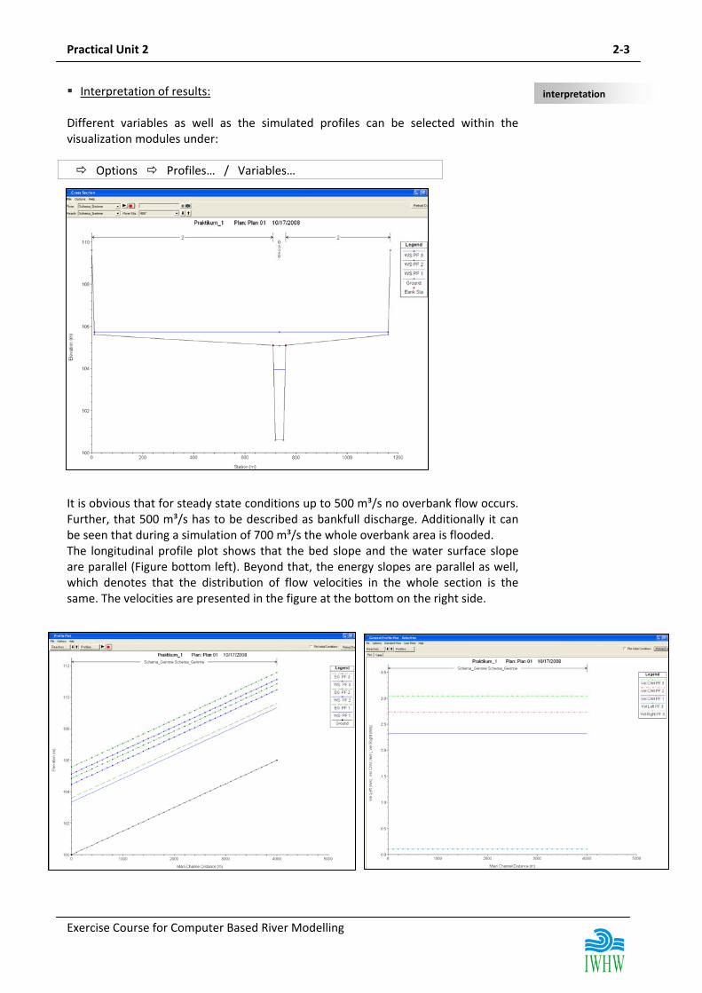
Interpretation of results: Different variables as well as the simulated profiles can be selected within the visualization modules under: Options Profiles… / Variables… It is obvious that for steady state conditions up to 500 m³/s no overbank flow occurs. Further, that 500 m³/s has to be described as bankfull discharge. Additionally it can be seen that during a simulation of 700 m³/s the whole overbank area is flooded. The longitudinal profile plot shows that the bed slope and the water surface slope are parallel (Figure bottom left). Beyond that, the energy slopes are parallel as well, which denotes that the distribution of flow velocities in the whole section is the same. The velocities are presented in the figure at the bottom on the right side.

interpretation



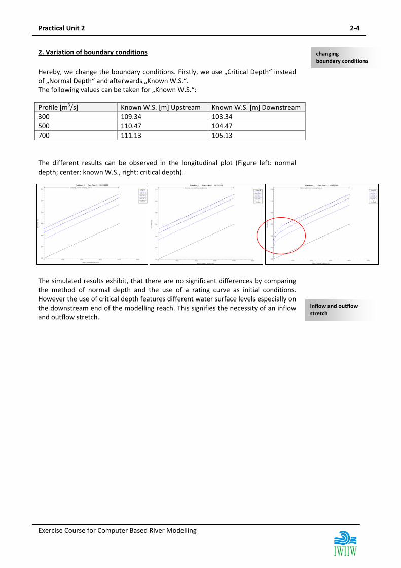
2. Variation of boundary conditions Hereby, we change the boundary conditions. Firstly, we use „Critical Depth“ instead of „Normal Depth“ and afterwards „Known W.S.“. The following values can be taken for „Known W.S.“:

The different results can be observed in the longitudinal plot (Figure left: normal depth; center: known W.S., right: critical depth). The simulated results exhibit, that there are no significant differences by comparing the method of normal depth and the use of a rating curve as initial conditions. However the use of critical depth features different water surface levels especially on the downstream end of the modelling reach. This signifies the necessity of an inflow and outflow stretch.

Profile [m3/s] Known W.S. [m] Upstream Known W.S. [m] Downstream 300 109.34 103.34 500 110.47 104.47 700 111.13 105.13

changing boundary conditions

inflow and outflow stretch



3. Changing options in steady state flow analysis Implementation of hydraulic boundaries „encroachments“: In the options menu for steady state flow analysis Options

the so called hydraulic boundaries “encroachments” can be defined. This allows the user to perform a floodway encroachment analysis. Once a reach is selected, the user can enter a starting and ending river station to work on. By default, the program selects all the sections in the reach. For the practical unit we select cross‐section 30 as upstream and cross‐section 20 as downstream boundary. Next, the user should select a profile number to work on. Profiles are limited to 2 through the maximum number set in the currently opened flow data. In this practical unit we set encroachments for profile 3 (700 m³/s). The next step is to enter the desired encroachment method to be used for the currently selected profile. The available encroachment methods in HEC‐RAS are:

Method 1 ‐ User enters right and left encroachment station Method 2 ‐ User enters fixed to width Method 3 ‐ User specifies the percent reduction

in conveyance Method 4 ‐ User specifies target water surface

increase Method 5 ‐ User specifies target water increase

and maximum change in energy

Set selected range (Left Station = 710 m; Right Station = 760 m). Once the encroachment method is selected, and its corresponding data are entered, the user should press the “Set Selected Range”‐button.

encroachments



Results and Conclusion: The results of the modified simulations are presented at the bottom of the page. Up to bankfull flow no influence of the encroachments on the water surface level can be seen. In contrast, for the 700 m³/s discharge simulation a significant influence on hydraulics is recognisable. In the upstream section of the encroachments the water depth considerably increases and the mean velocities decreases caused by backwater effects. In the river stretch with no overbank flow an acceleration of discharge happens (continuity equations) in combination with a lowering of the water surface level. Downstream of the encroachments a transition to the normal steady state conditions, as it was documented before, can be seen. Important: Always check the plausibility of your modelling result!! To control the flow regime check the Tables (Froude number < 1).



4. Modification of geometry Local change of bed slope: Till now, all computations dealt with subcritical flow regime (Froude number < 1). The following example shall demonstrate the transition from supercritical to subcritical flow due to changes in bed slope. Therefore a river stretch with three different slopes will be investigated. Firstly, it is shown how to raise the bed level elevation. Afterwards a prepared geometric data set will be loaded for the simulations. Raising or lowering of bed elevations of a cross‐section can be done in Options Adjust Elevations

For the following calculation a prepared geometric data set must be loaded (filename: Praktikum_1.g04). File New Geometry Data Name: Praktikum_2

File Import Geometry Data HEC‐RAS‐Format

select file and set to SI‐Units!!! The longitudinal plot should look like the figure to the right. At last, the steady state flow data must be adapted to the new geometry: Number of Profiles: 1

PF1: 300 Reach Boundary Conditions:

Downstream: Normal Depth = 0.0028 Upstream: Normal Depth = 0.01 We start the calculation with the flow regime „Subcritical“, followed by “Supercritical“ and finally by „Mixed“. The results should be controlled in the longitudinal plot . Additionally, we want to have a look at the critical depth: Options Variables Critical Depth Elevation anklicken

modification of bed slope



„Subcritical“ „Supercritical“ „Mixed“ As can be seen both, subcritical and supercritical do not succeed in simulating the hydraulic jump, because the criterion Froud number < 1 respectively > 1 is strictly kept.

hydraulic jump



Changes in bed elevation (simulation of local obstructions): This example simulates a small weir by raising the river bed in one of the cross‐sections. Therefore, we use the originally geometry of practical unit 1. The small weir is situated between cross‐section 2685 and 2710 and has its top in cross‐section 2700 with a height of 105 m a.s.l. To guarantee a trouble‐free calculation it is recommended to increase the number of cross‐sections in this area (cross‐section 2600 – 2800) by cross‐section interpolation (distance: 5 m, respectively 1 m).

local obstructions

Detail view„small weir“



Step 1: „Fixation“ of cross‐sections 2600, 2700, 2800 Options Rename River Station delete *

(Check: now these cross‐sections are plotted in the plan view in dark colour)

Step 2: Interpolation of cross‐sections with a distance of 5 m Tools XS Interpolation Between 2 XS’s…

Constant Distance: 5m

(Check: in plan view and longitudinal plot) Step 3: “Fixation” of cross‐section 2685 and 2710 (see step 1) and deletion of the

cross‐sections between 2685 and 2700 as well as 2700 and 2710 Tools XS Interpolation Between 2 XS’s…

Delete Existing Interpolated XS’s Step 4: Raising the bed levels of cross‐section 2700 to 105 m a.s.l (+ 0.95 m) lifting the bed level elevation at the stations

719 and 751 to 105

(Check: in longitudinal plot) Step 5: Interpolation of cross‐sections with a distance of 1 m between 2685 and 2710

(Check: in longitudinal plot and 3D‐plot) Step 6: Reduction in roughness‐values (for a better illustration of the hydraulic jump) Tables Manning’s n or k values

marking of the middle column and Set Values: 0.028 Step 7: Input of steady state flow data

PF 1 = 300 m3/s Reach Boundary Condition Up‐/Downstream: Normal Depth = 0.0015

Check of calculation in the longitudinal plot displaying the variables Water Surface, Energy Grade Elevation and Critical Depth Elevation. The effects of the changes in local bed level elevation on the water level shows a hydraulic jump downstream of the “weir” as well as the critical depth on top of the obstructions.



Changing river width (simulation of a river widening): In this example the width of the schematic channel will be increased in the cross‐sections 3000 – 3500 by 35 m on both sides: Altering the Positioning as well as the Bank Stations

(Check: in cross‐section plot and 3D‐plot)

Input of steady state flow data

PF 1 = 300 m3/s Reach Boundary Condition Up‐/Downstream: Normal Depth = 0.0015

Check of calculation in the longitudinal plot displaying the variables Water Surface, Energy Grade Elevation and Critical Depth Elevation.

river widening



The impact of the widening on river hydraulics is clearly visible (left figure): At the upstream end of the widening section a reduction of water surface level can be seen (e.g. flood protection) in combination with an increase of flow velocities. Further, a flattening of the energy slope is visible, which directly influences flow velocities (right figure) and bottom shear stress (sediment deposition). Additionally, different effects on hydraulics in relation to different discharges must be considered. Further, it should be once more mentioned that the examples of the practical units are results of schematic river reaches. In reality much more boundaries have to be considered.

Documents

PRACTICAL UNIT 2 exercise task - iwhw.boku.ac.at · on the input data of practical unit 1. The main focus in this unit is given to the The main focus in this unit is given to the