Practice Workbook - Bentley Userbentleyuser.se/2015_BUSdagar/Presentationer/Functional Components... · This workbook is designed for use in Live instructor-led training and for

Copyright © Bentley Systems, Incorporated DO NOT DISTRIBUTE – Printing for student use is permitted 1

Practice Workbook This workbook is designed for use in Live instructor-led training and for OnDemand self-study. The explanations

and demonstrations are provided by the instructor in the classroom, or in the OnDemand eLectures of this course

available on the Bentley LEARNserver (learn.bentley.com).

This practice workbook is formatted for on-screen viewing using a PDF reader. It is also available as a PDF

document in the dataset for this course.

Functional Components using

MicroStation CONNECT Edition

TRNC01998-1/0001

http://learn.bentley.com/







Using Multiple Cells - Functional

Components

This workbook contains exercises to place and work with parametric cells in your MicroStation CONNECT Edition

design. You will also learn the advantages to using Functional Components.

TRNC01995-1/0001



Description and Objectives

Course Description

In this workbook we will learn about functional components and parametric modeling. Then we will learn how to work with Parametric Cells.

Skills Taught

Why Functional Components are needed

What a Parametric Model is capable of

How you can leverage Functional Components skills

How to interact with Parametric Cells already placed

How to look up Parametric Cell Properties

How to modify a Parametric Cell already placed

What is scope of a Parametric Cell property: Instance and Definition

How to access a Parametric Cell Library

How to select and place Parametric Cell from a library


Why do we need Functional Components?

Functional Components and Parametric Modeling serve a common and specific purpose. Architectural, Engineering and Construction projects often

need parts that are similar in some respect like their function or basic geometry. But they are not exact replicas or even scaled copies of each other,

as they may differ only selectively in a few key aspects. E.g. a building or an elevated highway design would have large number of beams, columns

and girders that share similar geometry but vary in specific dimensions like length, width and cross sectional area.

The example above shows two reactor vessels of different height, diameter, nozzle positions etc. but other aspects like the pitch of the ladder steps,

nozzle sizes, railing height and walkway width would remain the same. Thus one is not a scaled copy of the other and hence unless we have a way

of making selective changes, we will have to model them both individually – practically doubling the design effort.


What can a parametric model do?

In the above example - in spite of all the differences – there are noticeable similarities. A parametric model captures this essential similarity that

remains unchanged while keeping room for the variations needed by specific instances. This ‘generic’ design needs to be created only once, to

which specific values can be assigned while creating instances. Further, sets of commonly used values can be created to form a ‘library’ or

‘catalogue’ of standard parts. E.g. here is a catalogue of risers used in sewer systems

Additionally, a parametric model also provides the flexibility needed at the initial exploratory-evolutionary stage of the design process. It can be

altered quickly and meaningfully to explore ‘what if’ scenarios of form, function or even economy and aesthetics; thereby arriving at the best

alternatives quicker.


How can we leverage parametric modeling skills?

One need not be an expert to leverage the benefits of parametric modeling. Parametric models created and shared by others can be accessed and

used by anyone for placement in a design. It takes little training to modify them to suit specific requirement or define your own ‘Variations’ of it. In

this course we will learn how to access, use and modify Parametric models.


Placing Parametric Cells

1. Open the file Bridge Superstructure.dgn. It shows a typical bridge span. Outlines of the piers and the deck are shown. The deck is to be

supported by beams, two of which are already placed. We will:

a. correct the height of Beam A

b. correct the length of Beam B

c. Place four more beams of correct length and cross section along the lines given. We will use a Parametric Cell library of pre-stressed

concrete beams for this.


2. To correct the height of Beam A:

a. Select Beam A.

b. In the Properties Pane, expand the General section.

c. Among the properties and values listed, note the current value of Variation is G72.

d. Click the drop down list arrow to see the list of possible variations.

3. From the list select G63. Note the beam now correctly fits between the pier top and bottom of the deck.

What did we just do? We modified a Parametric Cell! Note we have not yet attached any cell

library, but the beam (a parametric cell named Type V) already knows the possible variations it

has to offer. Replacing one variation of a standard component by another in a design is very

convenient with Parametric Cells. In it were an ordinary cell, attaching a cell library is necessary

for its replacement. With Parametric Cells we can do that without attaching the cell library!

2. To correct the length of Beam B.

a. Select Beam B.

b. In the Properties Pane, note property Len is listed in the Type V section. Its current value is listed as 60 units.

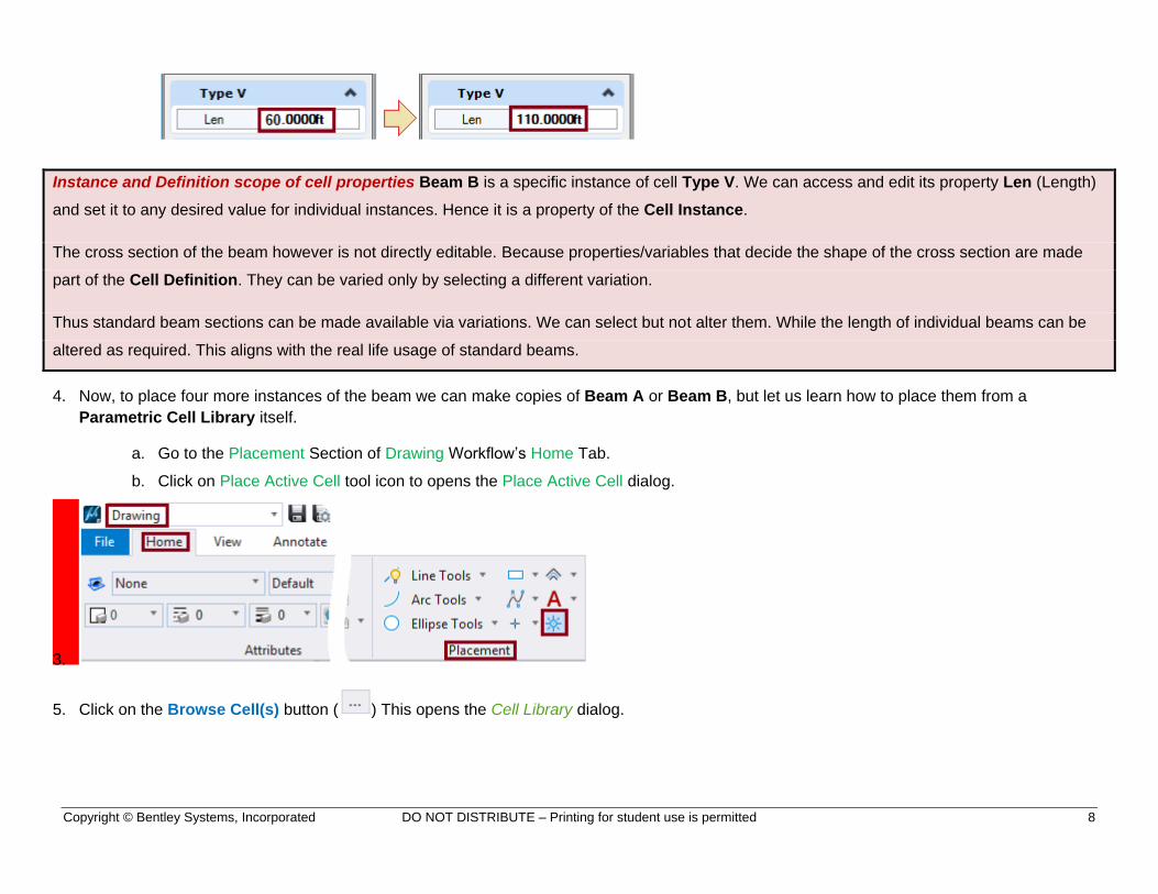
c. Change the value to 110 – the desired length. Note the beam now correctly reaches up to the second pier.


Instance and Definition scope of cell properties Beam B is a specific instance of cell Type V. We can access and edit its property Len (Length)

and set it to any desired value for individual instances. Hence it is a property of the Cell Instance.

The cross section of the beam however is not directly editable. Because properties/variables that decide the shape of the cross section are made

part of the Cell Definition. They can be varied only by selecting a different variation.

Thus standard beam sections can be made available via variations. We can select but not alter them. While the length of individual beams can be

altered as required. This aligns with the real life usage of standard beams.

4. Now, to place four more instances of the beam we can make copies of Beam A or Beam B, but let us learn how to place them from a

Parametric Cell Library itself.

a. Go to the Placement Section of Drawing Workflow’s Home Tab.

b. Click on Place Active Cell tool icon to opens the Place Active Cell dialog.

3.

5. Click on the Browse Cell(s) button ( ) This opens the Cell Library dialog.


4. From the File Menu, go to Attach File. In the file browse dialog that opens, select the file MyGirders Library.dgn. When the library is

attached, a list of Cells in the library and details like Name, Type etc. is now seen.

5. Double click on cell Type V. This opens the Place Parametric Cell Dialog.

6. Expand the Variations drop down list. This shows two Variations G63 and G72. Select G63. This displays the Properties of G63 split in two

categories:

a. Instance Properties: Titled Type V, this lists only one property Len displayed in bold, which can be edited.

b. Definition Properties: Titled Variables, these show the variable names and values in gray indicating these are for reference only and

cannot be altered as they define the standard section of the beam.


7. Change Len to 110. A Type V beam of length 110 ft and height 63 inch is now attached to the cursor, ready for placement. If necessary,

rotate the AccuDraw compass to Top plane to reorient the beam and snap it in to position.

8. Place four more beams to complete the support for the deck.

9. To see the bridge span in its entirety, turn on Levels Bridge Deck and Piers.


Power of Parametric Modeling The power of Parametric Cells lies not only in their ease of modification, but also the selective access to data they

allow. Here the variables controlling the shape of cross section were visible, but not editable to adhere to standards. Judiciously controlling access

to properties and variables, is part of a good parametric cell design!

What Next? We will look inside a Parametric Model/Profile and learn two important underlying concepts that make it work – Constraints and

Degrees of Freedom. They help us embody the design intent into a Parametric profile so it behaves and can be controlled in a way we want.







Parametric Profiles – What Makes Them

Work

This workbook contains exercises to learn how to set Constraints and use Variables in Parametric Profiles.

TRNC01996-1/0001




In this workbook we will learn about constraints and degrees of freedom. Throughout the course, we will restrict ourselves to 2 Dimensional or

planar Parametric Designs also called as Parametric Profiles. For variables, we will learn how to use the constraints that we applied earlier, and

also how to select, apply, and create variables.

Skills Taught

What are Constraints and how to display and inspect them

What is Degree of Freedom (DoF) and how to find it

How Constraints affect the DoF

What is a well constrained profile

How to Auto impose Constraints

How to selectively display geometric and dimensions constraints

How to find more about a constraint

What are Variables, Values, Expressions and Variations

How to access the Variables defined in a DGN Model

How to select and apply a Variation

How to create a Variation


Constraints and Degrees of Freedom

1. Open the file Constraints and DoF.dgn and open the model Quadrilateral to Square It shows successive stages of the process of changing

an arbitrary quadrilateral (any four sided shape) to a 50 x 50 square with a horizontal base.

The above quadrilateral to square transformation is done by imposing a series of conditions on the successive stages. Such conditions are

called Constraints. They could be Geometric or Dimensional.

2. Go to the Constraints Tab of Drawing/Modeling Workflow to see all the available Constraint Tools. You might find many of the constraint tool

names and even their icons self-explanatory. Examples are Parallel, Perpendicular, Tangent, Fixed, and Concentric.

3. From the View Attributes Menu, go to Markers setting and turn on the display check boxes. Blue glyphs appear in the file, each representing a

constraint imposed.


Note the glyphs can be easily matched with the corresponding constraint tool like -

Fixed ( ), Parallel ( ), Perpendicular ( ), Equal ( ) etc.

Having separate check boxes for Geometric and Dimensional constraints allow you to hide one type of constraints while displaying the other.

This is particularly helpful in getting an uncluttered view of complex profiles.

4. Move the cursor over the constraint imposed at each stage. This displays more information about the constraint as follows

a. The glyph gets highlight in orange

b. The elements it applies to also get highlighted in orange

c. A pop up text displaying the name of the constraint appears


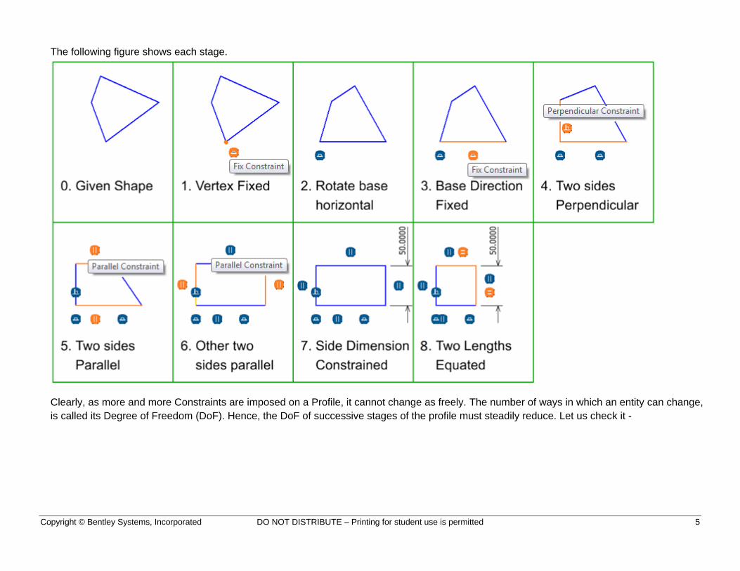
The following figure shows each stage.

Clearly, as more and more Constraints are imposed on a Profile, it cannot change as freely. The number of ways in which an entity can change,

is called its Degree of Freedom (DoF). Hence, the DoF of successive stages of the profile must steadily reduce. Let us check it -


5. From the Constraint Utilities Section in the Constraints Tab, click on the Degree Of Freedom Tool.

6. Click on the successive stages of the profile. DoF of each stage gets displayed at the center of the profile.

Try to mentally match the DoF displayed and the number

of ways that profile can vary. For example, stage 6 has all

else fixed, except the length and height of the rectangle

formed. Thus it has two degrees of freedom.

Note the color code used in the display. Entities that are

not free to move, are shown in Orange, while those not

fully constrained yet are displayed in Blue. Text

displaying DoF too follows this color code. DoF = 0 is

shown in orange, while all other values of DoF are

displayed in blue.


The table below gives a summary of this process of constraining a profile from the DoF point of view.

Stage DoF Constraint Added Condition imposed

1 6 Fixed Location of a vertex Fixed

3 5 Fixed Orientation of the base Fixed

4 4 Perpendicular Orientation of a side fixed (perpendicular to the base)

5 3 Parallel Orientation of top side fixed (parallel to the base)

6 2 Parallel Orientation of right side fixed (parallel to the left side)

7 1 Dimension Dimension of right side (height) fixed to be 50 units

8 0 Equal Length of top side (length) fixed (to be equal to the right side)

The final step brings down the DoF of the profile to zero. Such a profile is said to be well constrained. Well constrained profiles can still change

when the dimensions are edited. But such changes are predictable and are consistent with the design intent for well-designed profiles. For example

we can change the dimension to say 75 and still be sure it will remain a square!

Design Intent and constraints In the above example, there could have been several different ways of turning the quadrilateral into a square. For

example instead of making the two sides Equal. In step #8, we could have imposed a dimensional constraint making the top edge length = 50. This

would have made a 50 x 50 square too. But when we vary a dimension it will not remain a square! So if we wanted to model a square, imposing the

Equal constraint aligns better with the design intent of creating a square.

7. Right click on the dimension in step #8. This brings up a pop-up menu.

8. Select Edit Dimension from the pop-up menu. This brings up a Text Box displaying the current value. This can be overwritten with any desired

value.

9. Enter 75 in the Text Box and press Enter (or click outside of the Text Box). Note the profile changes to a bigger 75 x 75 square.

Had we used an additional dimensional constraint instead of the Equal constraint, this change would have resulted in a 50 x 75 rectangle!



Using the Auto Constraint tool

The profile used for this exercise was simple with only a few constraints, but real life profiles can have a large number of Constraints. Imposing each

of those individually, could be time consuming. In such a case, the basic shape is drawn as close to the desired profile as possible and the Auto

Constraint Tool is used on it.

This tool –

a. examines all the constituent elements (lines, arcs, circles etc.) in the shape

b. finds all possible interrelationships between these elements like parallelism, perpendicularity, tangency etc.

c. adds corresponding constraints.

Needless to say, this can save a lot of time.

1. In the same file, open the model Box Girder Profile It shows two cross sections of a box girder. One is a Parametric Profile while the other is a

plain shape. Turn on display of constraints if they are not visible.

2. From Constraints Tab start the Auto Tool.

3. Click on the outer shape of the girder on the right. Several constraint get displayed around the shape. This is a preview which can be rejected

with a reset (right click).


4. Accept with a data point anywhere. This confirms the constraints.

5. Similarly, Auto Constraint the inner shape of the girder on the right.

What is Next? In the next module we will learn about Variables, Expressions and Variations, which help model the dimensional data of a profile

and implement standardization with commonly used sets of dimensions.


Variables, Expressions and Variations

In this section, we will learn how to use the constraints that we applied earlier, and also how to select, apply, and create variables.

1. Open the file Girder 01.dgn and go to Model Profile01. It shows a section of a bridge girder.

2. Open the View Attributes menu and the Markers setting.


3. Click on the Constraints check box to enable the Geometry and Dimensional check boxes.

4. Select the Geometric check box to display the Geometric Constraints added to this profile. But keep Dimensional turned off.

5. The large number of constraints this complex profile carries may seem overwhelming at first. But you can find more about a specific constraint

by starting the Selection tool and moving the cursor onto any glyph. This highlights the relevant elements and a paired glyph if any, e.g. Parallel

constraint shows glyphs for both the lines. A popup label is also displayed as shown.


6. Now turn off the Geometric check box and turn on the Dimensional check box to display the dimensional constraints.

Note the dimensions are labeled, e.g. Thk for thickness, TS for top span etc. These are called Variables because their Value can be varied to

change the design. They can be managed (define, delete, access and edit) from the variables dialog.

7. From Constraint Utilities section in the Constraints tab, click the Variables icon (fx) to open the Variables dialog.


It shows Variables, their Values and Variations which are specific combinations of variable values. (If you do not see the list of variables,

click on Local Variables to expand the list.)

Why use Variables? Variables are placeholders that can be assigned different values. There are several advantages of using them.

Identification / Description: Role played by a dimension can be easily conveyed with a meaningful variable name e.g. in the list of numerical

values, we can quickly identify the top span of the girder as ‘TS’. A variable name can be made as descriptive as we want. E.g. ‘SideSlope’ used for

the angle of inclination of the lateral sides of the girder.


Propagate change: Some dimensions (length or angle) could be repeated in several places in a design and they need to change together.

Changing individual dimensions is not only cumbersome but also error prone. When labeled with the same Variable, any change in its value is

quickly propagated to all dimensions it is linked to. E.g. changing the value of Variable ‘Thk’ would uniformly change the girder thickness at top,

side, bottom etc.

Maintain Interrelationships – Dimensions in a design are often interrelated and any change in one requires a specific change in others. For

example, changing the outer dimension, must update the inner cavity of the girder. Their interrelation is captured in the Expression: ‘BaseInside =

B – d’

Why are they called ‘Local’ Variables? The variables defined are visible and applicable only within the DGN Model they are defined in. Thus they

are called ‘Local’.

8. Select Variable BaseInside in the Variables dialog. Note an Expression ‘B – d’ appears in its properties as shown below. Thus any change in

the value of Variable ‘B’ or Variable ‘d’ will also bring about a change in the value of variable BaseInside.


The Expression used above is simple, but more complex expressions can be composed using Expression Builder.

9. Click the button given against the Expression. Expression Builder opens. It lists all the Local Variables, Functions and constants; as well as the

operators. Using Arithmetic~, Relational~ and Logical ~ Operators on these, complex expressions can be formulated.


What are Variations? Often certain combinations of Variable values are preferred because of common practice or frequent usage or industry

standards (e.g. like a range of sizes of a part offered in a catalogue). Variations store such sets of Variable values and apply them to a Parametric

Model. The Parametric Model adopts these numerical values and morphs into that specific Variation.

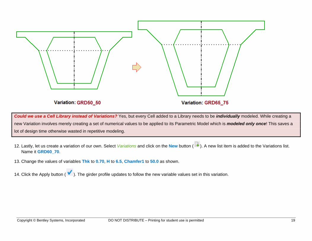
10. From the Variations list, select GRD50_50 and then GRD65_75. Note the values of the variables listed in Properties. Note the values of Thk, H,

BaseInside, and Chamfer1, d change as we go from one variation to the other (marked with an in the figure below).


11. Now select variation GRD65_75 and click the Apply button ( ) Note this alters the girder profile, because the variables that control the shape

and size of the profile, now take the values prescribed in GRD65_75.


Could we use a Cell Library instead of Variations? Yes, but every Cell added to a Library needs to be individually modeled. While creating a

new Variation involves merely creating a set of numerical values to be applied to its Parametric Model which is modeled only once! This saves a

lot of design time otherwise wasted in repetitive modeling.

12. Lastly, let us create a variation of our own. Select Variations and click on the New button ( ). A new list item is added to the Variations list.

Name it GRD60_70.

13. Change the values of variables Thk to 0.70, H to 6.5, Chamfer1 to 50.0 as shown.

14. Click the Apply button ( ). The girder profile updates to follow the new variable values set in this variation.


What Next? Profiles that vary with Variables and Variations are useful in 2 D design, but more often solids that vary in a similar manner are

required. The next step would be to take a parametric 2 D profile and create a Parametric Solid from it, that inherits it’s Variables, Variations,

Expressions and the parametric capability.







Creating Parametric Solids and

Parametric Cell Libraries

This workbook contains exercises to learn how to create Parametric Solids and Parametric Cell Libraries.

TRNC01997-1/0001




In this module, we will learn about using Parametric Solids and Features. We will also learn how to create a Parametric Cell.

Skills Taught

Create Parametric Solids

Add Parametric Features

Identify Tools Settings that take Variable Values

Apply Variations to a Parametric Solid

Impose Geometric Constraints on a given Shape or Complex Shape

Create Variables and initialize them with Active Values

Impose Dimensional Constraints

Create a Parametric Solid

Create Variations

Set Model Properties to place it as a Parametric Cell


Transition into 3 D

So far we have seen two dimensional parametric profiles i.e. planar shapes that can be parametrically changed or controlled. This ability in itself is

useful of course, but we can also use such profiles to create solids and features. And the best part is, such solids and features inherit the parametric

behavior of the original profiles.

1. Open the file Girder 02.dgn and go to Model Box Girder Profiles. It shows a section of a bridge girder.

2. From the Create Solids section of the Modeling workflow, start the Extrude tool. We will use this tool to create a solid by extruding the profile.

Some convenient View Rotation Mode like Isometric can be chosen for convenience.

3. In the Tool Setting turn on the check boxes Parametric and Distance. The (x) beside Distance indicates that it can be assigned the value of

any Variable defined in the file.


4. Click the (x) icon beside Distance to open the list of Variables and their Values.

5. Select the Variable (L) and click OK to assign its Value to setting Distance of the Extrusion tool. Note the value of L is intentionally kept low

here for ease of viewing in Fit View mode.

6. Click to select the outer profile and click a data point to define the direction and create the solid of extrusion. Note this is a solid block without the

central cavity.


7. From the Features section of Solids tab of Modeling workflow, start the Cut tool. We will use this tool to create the cavity at the center, which is

also parametric. Set the following values:

Setting Option

Cut Method Inside Profile

Cut Direction Forward

Cut Mode Through

Profile Hide

8. Switch to the Wireframe Display Mode so that the inner profile can be seen. Select the solid and then the profile to execute the cut operation.

Now, let us check if the solid thus obtained is still governed by the Variations that were defined in the profile.


9. In the Variables dialog, select different Variations (previously defined for the 2D Profiles) and click the Apply () button. Note the solid changes

according to the Variation applied.


Lastly, we will see how to view the profile used in generating such Parametric Solids.

10. With the Selection tool, click on the solid. This displays the Profile icon ( )

11. Right click the Profile icon and select Show Input Element from the right click menu. The original profile gets displayed along with the solid.

This is apparent from the Geometric or Dimensional constraints that become visible if their display is turned on in View Attributes

Another route to Parametric Solids Instead of starting from a Parametric Profile (2 D) and using a Solid Creation tool, one can also start from a

Primitive Solid like Slab, Cylinder, Sphere, Cone, Torus etc. Parametric Features may then be added to these as needed. This approach might be

quicker for Parametric Solids with simple cross sections.

What Next? Now that we have created both 2 D Profiles and 3 D Solids, that can be varied using Variables and Variations defined in their parent

DGN Model, next we will see how to share them so they can be placed in other files. Namely, we will see how to create Parametric Cells from such

Profiles and Solids.


Parametric Cell Models and Cell Libraries

Let us create a parametric cell for a standard steel section commonly used in construction. We will keep the geometry simple, so as to focus on the

process.

1. Open the file Steel Section.dgn This file has several models; which progressively show successive stages of creating a Parametric Cell. They

can be worked on sequentially or any step can be skipped to by selecting the appropriate model.

a. Model 00 Notation – shows the notation indicating the role played by each of the variables used

b. Model 01 Complex Shape – holds a plain complex shape to which constraints can be added

c. Model 02 with Geometric Constraints – shows the profile with geometric constraints

d. Model 03 With Dimensional Constraints – shows the fully constrained profile with dimensional constraints added

e. Model 04 Parametric solid – shows the solid obtained by extruding the profile with length as a parameter

f. Model L Section – the finished model that can be placed as a parametric cell

2. Open Model 00 Notation. It shows a standard ‘L’ steel section. Note instead of numerical dimensions it uses variables a, b, r1, r2, t etc. These

are the names of the variables that will later drive the parametric profile and the subsequent parametric solid.


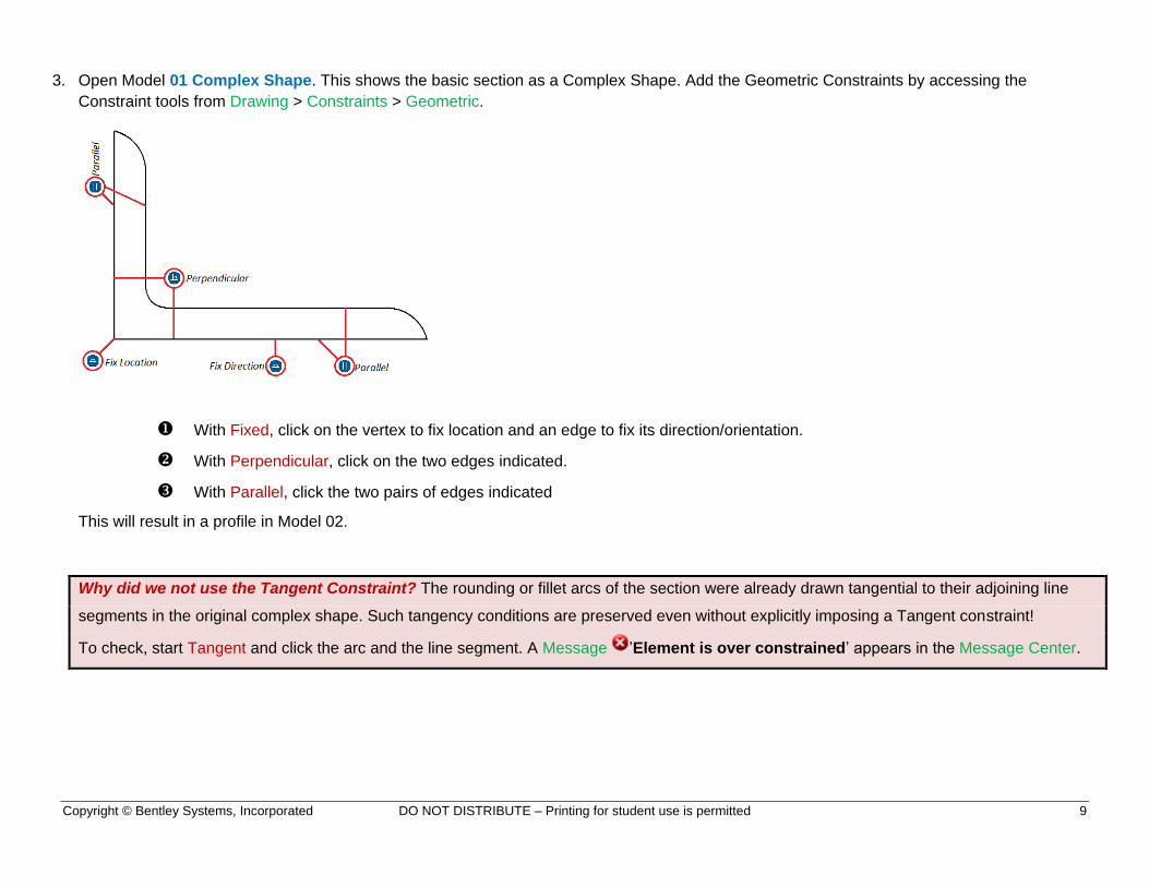
3. Open Model 01 Complex Shape. This shows the basic section as a Complex Shape. Add the Geometric Constraints by accessing the

Constraint tools from Drawing > Constraints > Geometric.

With Fixed, click on the vertex to fix location and an edge to fix its direction/orientation.

With Perpendicular, click on the two edges indicated.

With Parallel, click the two pairs of edges indicated

This will result in a profile in Model 02.

Why did we not use the Tangent Constraint? The rounding or fillet arcs of the section were already drawn tangential to their adjoining line

segments in the original complex shape. Such tangency conditions are preserved even without explicitly imposing a Tangent constraint!

To check, start Tangent and click the arc and the line segment. A Message ’Element is over constrained’ appears in the Message Center.


4. Open Model 02 With Geometric Constraints. The general shape of the section is now defined by the geometric constraints. We will refer to

this as a profile. The size of the profile however is still not fixed by any quantitative constraints. We will use Dimensional constraints to do that.

5. Open the Variables dialog from Drawing/Modeling > Constraints > Constraint Utilities.

6. Select Local Variables and click the New Button ( ), to create the variables listed in the table.


Note each variable is initially set to a default value of 1.0. But this can be changed by entering the Active Values shown.

Variable Active Value

a 30

b 20

t 3

r1 4

r2 2

The settings Type [= Distance], Scope [= Definition], Expression [= None] are same for all the variables. All these variables help predefine

standard section shapes, not to be edited for instances. Hence Scope = Definition.

7. For Variables {a, b, t} set Display = Visible. Though not editable, these are still of interest during placement. For Variables {r1, r2} set Display =

Hidden, because these are not significant in design considerations.


8. Start Dimension Element tool from Drawing/Modeling > Constraints > Dimensional to add the dimensional constraint:

Click on the base of the profile to dimension it. This opens a text box with a drop-down List.

Expand the drop-down list. All the variables defined are listed in it.

Select Variable (a) to assign it to this dimension.

Click elsewhere or press Enter to accept this assignment. Now this dimension of the profile will be driven by the variable (a).


9. Similarly, assign the variables to other dimensions of the profile as shown: This will result in a profile in Model 03.

10. Open Model 03 With Dimensional Constraints. It shows the profile adequately constrained to retain its shape and size. It can now be extruded

into a parametric solid.

11. Define a new Variable (L) with Active Value 500.00 to drive the length of the extruded solid.


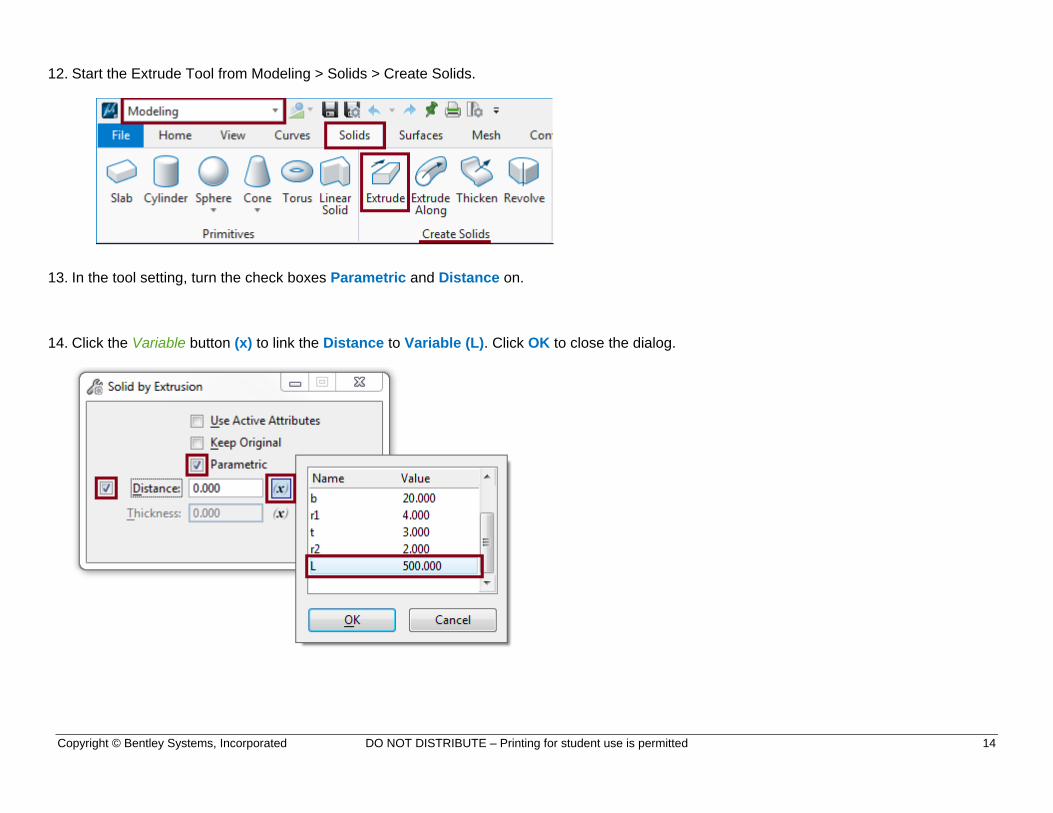
12. Start the Extrude Tool from Modeling > Solids > Create Solids.

13. In the tool setting, turn the check boxes Parametric and Distance on.

14. Click the Variable button (x) to link the Distance to Variable (L). Click OK to close the dialog.


15. Select the profile and extrude it. Move the solid to locate any one of its vertices at the Model Origin (0, 0, 0).

16. In the Variables dialog, select Variations and click the New button ( ) to create the following three Variations.

VARIATION a b t r1 r2 L

30 x 20 x 3 30 20 3 4 2 500

30 x 20 x 4 30 20 4 4 2 500

40 x 20 x 4 40 20 4 4 2 500

17. Apply any of these Variations by selecting it and clicking the Apply button ( ). The solid changes to conform to the Variation. So we have a

parametric solid now. Next we will make it into a parametric cell.

At this stage Model 03 content is equivalent to Model 04 Parametric Solid. So either one can be used for creation of a parametric cell.

18. Open Model 04 Parametric Solid


19. In the Properties Pane, expand Cell setting, to set

Can be placed as Cell = True

Cell Type = Parametric

Note in the Variable setting, the variables defined in the model are listed along with their current or active values.

As covered in the previous courses, this file can now be attached as a cell library to another file and this Model can be placed as a parametric

cell. Such a cell will have its Variations accessible from any of its instances.

At this stage Model 04 content is equivalent to Model L Section. So either one can be used as a finished cell Model.


Cell and Model Origin: During cell placement dynamics, typically one point/vertex of the cell remains attached to the cursor, thereby serving as a

sort of handle for the cell. It is called the Cell Origin. We can make any convenient point within the cell geometry - say a vertex or even an

abstract point - as the cell origin by locating it at the origin (0, 0, 0) of its parent model.

20. Open model Channel Section. It shows a standard steel channel modelled as a Parametric Solid. From the Variables dialog, several Variations

can be seen.

21. Select the Model in the Models dialog, so its properties are seen in the Properties pane.

22. In the Cell section, make appropriate changes so that the Model can be placed as a Parametric Cell.

23. Move the solid to locate any desired point in it at (0, 0, 0) so that it serves as the Cell Origin. This File - now a Cell Library - has two standard

steel section cells. They have predetermined sections which cannot be edited for instances placed. However, they can be selected from a range

of standard Variations. The length of these cells can be changed from instance to instance. This is akin to the real life practice of procuring

standard sections and cutting pieces of suitable length as needed on site.

What Next? More models that can be placed as parametric cells can be created, expanding this Cell Library. For additional practice, a standard

‘I’ section shape is provided in Model I Section. Required Variables and Variations to be implemented are given in the table below.

Documents

Practice Workbook - Bentley Userbentleyuser.se/2015_BUSdagar/Presentationer/Functional Components... · This workbook is designed for use in Live instructor-led training and for