Embed Size (px)
Citation preview

Department of Economic History
Stockholm University 2015
Stockholm Papers in Economic History No. 17
Pre-industrial population and
economic growth: Was there a
Malthusian mechanism in Sweden?
Second version
By Rodney Edvinsson
First version presented at Higher Seminar, Department of Economic History, Lund, 22 January 2014 (http://www.lusem.lu.se/media/ekh/seminarie-paper/paper111.pdf).
Stockholm Papers in Economic History, No. 17
2015
Web address of the WP-series: http://swopec.hhs.se/suekhi
The working papers are reports of ongoing studies in economic history at Stockholm
University. Authors would be pleased to receive comments.
Department of Economic History
Stockholm University
SE-106 91 Stockholm
Sweden

Pre-industrial population and economic growth:
Was there a Malthusian mechanism in Sweden?
Rodney Edvinsson1
Stockholm Papers in Economic History, No. 17
2015
Abstract
This study examines whether there was a Malthusian equilibrium mechanism in Sweden 1630–
1870. A unique data set on harvests, deaths, marriages and births is used to calculate cumulative
elasticities of vital rates with respect to harvest. While earlier studies have mostly focused on the
impact of real wage, this study contents that the calorie content of harvests is more related to
Malthus’ concept of the ‘produce of land’. It finds that there indeed was a response of vital rates to
harvest fluctuations, but there were important structural breaks. While positive checks attenuated
after 1720, preventive checks were strengthened. After 1870 preventive checks disappeared, even
if positive checks existed up to 1920. The results are robust to different models – DLM, ARMAX
and SVAR – and trend specifications.
JEL-classification: N13; N33; N53
Key words: demography; Maltus; mortality; fertility; economic history
1 Department of Economic History, Stockholm University, SE-106 91 Stockholm, and Swedish Collegium for
Advanced Study, Uppsala University. E-mail: [email protected] and

1. Introduction
The relation between population and economic development has been a central theme in
economic and social theory since the eighteenth century. The question of the causal
connection between economic and population growth in agrarian society is still unresolved.
There are two opposing interpretations. While Malthusians emphasise diminishing returns on
natural resources, producing mortality crises, their critics point out that population growth by
itself generated advances in technology.
The unified growth theory, which aims to model both technological progress and
demographic transition in the eighteenth and nineteenth centuries endogenously, predicts that
while preventive checks were initially strengthened, positive checks were weakened once
technological progress took off.2 What exactly a Malthusian model entails is a topic for an
ongoing discussion, and there is no reason to interpret the Malthusian mechanism in just one
way. In fact, Mokyr and Voth suggest that the Malthusian model rests on two assumptions:3
1) that population growth reacted positively to living standards through preventive and
positive checks and 2) that living standard was negatively related to the size of the population.
They contrast two Malthusian versions against each other. In its strongest form, it predicts
stagnant per capita income without shifting mortality and fertility schedules and stagnant
population in the absence of technological advance. In its weaker version, it accentuates
equilibrium mechanisms, i.e. the positive and preventive checks on population rather than the
specific outcomes.
2 Galor and Weil (2000); Pfister and Fertig (2010).
3 Mokyr and Voth (2008), pp. 14–15.

The analysis of the development of preventive and positive checks is highly dependent on
which variables are chosen and not only on the statistical model. Earlier international research
on the effect of economic stress on the population in the pre-industrial period has largely
relied on real wages or grain prices as indicators of living or nutritional standards,4 but the
approach is problematic. Malthusians often point to the development of real wages, which fell
from the late Middle Ages to the early nineteenth century, to advance their main proposition
that population growth outpaced production.5 Anti-Malthusians tend to disagree.
6 Maddison
contends that wages cannot be used as indicators of living standards since they do not
represent a macroeconomic variable.7 The volatility in grain prices was also affected by
market integration, not only by harvests.8 While there was a strong correlation between
movements in grain prices and harvests in the early modern period, this relation attenuated
during the nineteenth and twentieth centuries due to improved international market
integration. Recently, Dribe, Olsson and Svensson demonstrate that at the local level in
southern Sweden, grain output had a different impact on mortality than grain prices, since the
latter reflected conditions in surrounding areas.9
This paper utilises recently constructed annual series of vital rates and harvests to estimate
the elasticities of vital rates back to 1630. The whole period 1630–1870 is put into
4 Wrigley and Schofield (1989), pp. 368–384; Galloway (1988); Galloway (1994); Lee and Anderson (2002);
Nicolini (2007); Bengtsson and Broström (2011); Bengtsson and Ohlsson (1985); Dribe (2003); Crafts and Mills
(2009); Pfister and Fertig (2010); Chiarini (2010)’; Møller and Sharp (2014); Klemp and Møller (2015). Eckstein
et al (1984), and Larsen (1987), use a harvest series to investigate the impact on vital rates in Sweden, but this
harvest series is deficient for the period before 1865 (Edvinsson 2009). Dribe, Olsson and Svensson (2011),
analyse the mortality response to grain output (derived from tithes), but at the local level in southern Sweden.
5 Allen (2001), Clark (2007).
6 Persson (2008).
7 Maddison (2007), p. 308.
8 Edvinsson (2012).
9 Dribe, Olsson and Svensson (2011).

investigation, although a comparison is also made with 1871–1920. Harvests data are
transformed into the per capita production of calories. The appendix explains the data sources
in detail.
In this paper, the elasticities of vital rates are calculated as cumulative elasticities, since the
impact of harvest could be delayed. In the first step a simple distributed lag model (DLM) and
an ARMAX (auto-regressive moving average with exogenous input) model are presented.
Subsequently a structural vector autoregression model (SVAR) is applied to estimate
structural impulse response functions that can be given a causal interprestation.10
The
empirical evidence supports the view that there was a short-term Malthusian equilibrium
mechanism in the Swedish pre-industrial economy, even if the mechanism changed over time.
The question of whether there was a medium- or long-term Malthusian equilibrium
mechanism is, however, outside the scope of this study. A short-term mechanism does not
necessitates a long-term one, even if there is usually a connection between the two under
ceteris paribus.
2. An overview of the data
When comparing seventeenth century Sweden with other countries for which data on vital
rates exists, Sweden stands out for the occurrence of sever mortality crises. Figure 1 compares
the crude death rate in Sweden, England and north Italy. The English data, which are
reconstructed by Wrigley and Schofield, go back to 1541, and the data for north Italy to 1650.
In Sweden, the crude death rate was highest in 1710, at 84 per 1,000, the last outbreak of the
bubonic plague in Sweden. The second highest level was reached in 1651, at 72 per 1000. In
comparison, the highest level in England after 1541 was in 1558, at 54 per 1,000, and in north
10 Eickstein et al. (1984); Nicolini (2007).

Italy after 1650, in 1693, at 45 per 1,000. Still in 1773 the crude death rate rose above 50 per
1,000 in Sweden, while in England after 1558 the rate never rose above that level.
Figure 1: Crude death rate in Sweden, England and north Italy 1540–1870.
0
10
20
30
40
50
60
70
80
90
1540 1570 1600 1630 1660 1690 1720 1750 1780 1810 1840 1870
CDR, Sweden CDR, England CDR, North Italy
Sources: Galloway (1994), Edvinsson (2015), and Wrigley and Schofield (1989).
In Sweden there were two important breaks in mortality: around 1720, after the end of the
Great Nordic Wars, and around 1820, when Sweden entered its long period of peace and the
low point of death rates started to decline. Up to around 1720 the average crude death rate
was higher in Sweden than in England and north Italy. After 1720 it fell to the level in
England. According to the data of Wrigley and Schofield, English death rates did not decline
in the first half of the eighteenth century. After 1812, the Swedish crude death rate never rose
above 30 per 1,000, while that was the average level in north Italy up to the 1860s. By the
1840s the average crude death rate in Sweden fell below the average in England, despite that

Sweden was poorer. Mortality affected various groups differently,11
but that issue is not
considered here.
Figure 2 compares the volatility of the crude death rate in the three areas, measured as the
40-year moving standard deviation of the annual logarithmic change (choosing another
moving average period does not change the overall picture). The paths are clearly different in
the three areas. In 1650–90, volatility was equal in England and northern Italy, whereas in
Sweden it was substantially higher. While volatility decreased in England after 1690, and in
Sweden after 1720, the volatility in north Italy did not change. By the first half of the
nineteenth century, the volatility in Sweden decreased below the level in north Italy. Sweden
and England are therefore comparable in terms of a long-term decline in the occurrence of
mortality crises during the early modern period, but Sweden lagged 100 to 150 years behind
the development in England.
11 Bengtsson (2004).

Figure 2: The 40-year moving standard deviation of the logarithmic annual changes in crude
death rates in Sweden, England and north Italy.
0
0.05
0.1
0.15
0.2
0.25
0.3
1550 1600 1650 1700 1750 1800 1850
Sweden England North Italy
Sources: See Figure 1 and appendix.
The above comparison rests on the assumption that the underlying data are not biased, but
there are competing interpretations of the demographic development. The demographic data
for Sweden back to 1630 are based on an earlier study by the Swedish historian Lennart
Anderssom Palm. As explained in the appendix, the present study uses a revision to the series,
which upgrades the size of population and the vital rates especially for the earlier years.12
Razzel argues that the assumption of Wrigley and Schofield of a burial accuracy of 100 per
cent is unrealistic, and that the actual mortality levels could be much higher.13
He suggests
that in reality there was a decline in English death rates in the first half of the eighteenth
century, which would make the development in England comparable to Sweden.
12 Edvinsson (2015).
13 Razzel (1993), p. 752.

Figure 3 presents the development of the crude birth rate in the three areas during the same
period as in Figure 1. This is the period before the second phase of the demographic
transition, i.e. before fertility declined. Several Swedish historians argue that there was
another, hidden, demographic transition between the seventeenth and eighteenth centuries,
which increased the age for marriages. Larsson shows that the average age of first marriage
among women increased from around 24 years to around 26 years during the first two decades
of the eighteenth century and stabilised at this level after a temporary drop in the 1730s.14
Higher age of marriage indicates strengthened preventive checks. When compared to the quite
sharp medium-term fluctuations in England and north Italy the fall in the crude birth rate in
the early eighteenth century Sweden was not so large. However, Razzel argues that the rise in
birth rates in the eighteenth century according to the data of Wrigley and Schofield (see
Figure 3) could be spurious as well.15
14 Larsson (2006), pp. 145–146 and 205.
15 Razzel (1993), p. 745.
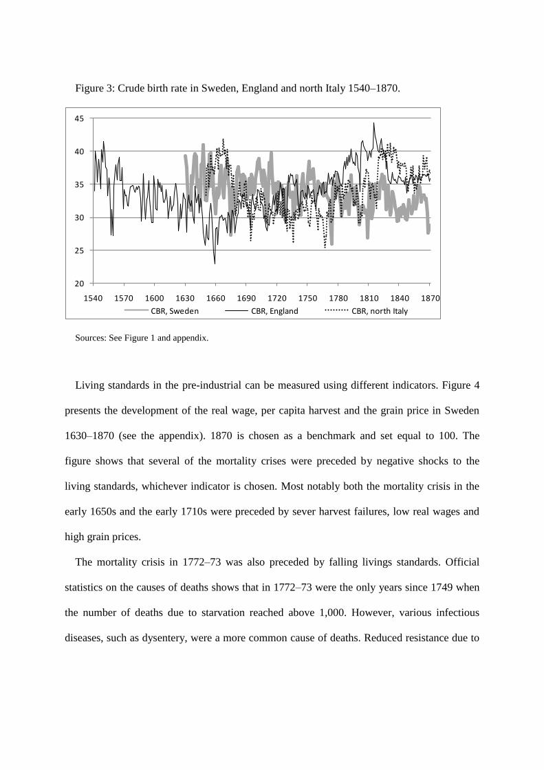
Figure 3: Crude birth rate in Sweden, England and north Italy 1540–1870.
20
25
30
35
40
45
1540 1570 1600 1630 1660 1690 1720 1750 1780 1810 1840 1870
CBR, Sweden CBR, England CBR, north Italy
Sources: See Figure 1 and appendix.
Living standards in the pre-industrial can be measured using different indicators. Figure 4
presents the development of the real wage, per capita harvest and the grain price in Sweden
1630–1870 (see the appendix). 1870 is chosen as a benchmark and set equal to 100. The
figure shows that several of the mortality crises were preceded by negative shocks to the
living standards, whichever indicator is chosen. Most notably both the mortality crisis in the
early 1650s and the early 1710s were preceded by sever harvest failures, low real wages and
high grain prices.
The mortality crisis in 1772–73 was also preceded by falling livings standards. Official
statistics on the causes of deaths shows that in 1772–73 were the only years since 1749 when
the number of deaths due to starvation reached above 1,000. However, various infectious
diseases, such as dysentery, were a more common cause of deaths. Reduced resistance due to

malnutrition and increased travels when people searched the country for food and work
contributed to the spread of these diseases.16
By the nineteenth century it is not as clear whether chocks to the living standards were
followed by mortality crises. Most notably the sever harvest failure in 1867 only slightly
raised mortality (mostly affecting northern Sweden17
), from 19 per 1,000 in 1865 to 22 per
1,000 at its peak in 1869. In comparison, in neighbouring Finland the outcome was different.
At the peak of the Finnish famine, in 1868, the crude death rate reached 78 per 1,000,18
a level
which in post-1630 Sweden was only surpassed once, in 1710.
Figure 4: Real wage (left scale), per capita harvest (left scale) and grain price (right scale)
1630–1870 (1870 =100).
0
50
100
150
200
250
300
350
4000
20
40
60
80
100
120
140
160
180
200
1630 1650 1670 1690 1710 1730 1750 1770 1790 1810 1830 1850 1870
Real wage Per capita harvest Grain price
Source: See appendix.
16 Willner (2005), p. 41.
17 Nelson (1988), p. 82.
18 Ó Gráda (2001), p. 576.

The indicators of livings standards tended to move together, but there are divergences
especially for the medium-term fluctuations. For example, the grain prices were at their
highest level, and real wages at their lowest level in the early nineteenth century.
Nevertheless, the development of per capita harvests or the crude death rates was different.
This study argues that per capita harvest is the superior indicator of nutrition standards. In
their study on the post-Malthusian economy in Scandinavia Klemp and Møller (2015, p. 2)
use real wage as an indicator of economic conditions, claiming it is “high-quality economic…
historical data”. However, for Sweden earlier research shows that there is a lack of strong
congruence between real wage and macroeconomic conditions. As Lennart Jörberg notes, ‘the
fall in the real wages of day-workers provides no information on the general economic
situation of agriculture during the later part of the eighteenth century’.19
It is likely that the
fall was counteracted by increased labour input per inhabitant. While real wage was very high
in 1690–1730, Morell demonstrates low levels of calorie intake in Swedish ‘hospitals’ in this
period.20
Using real wage as an indicator for living standards may therefore lead to wrong
conclusions concerning the relation between demographic indicators and economic
conditions.
In his original demographic theory Malthus related population growth to food production
rather than to per capita income or wages.21
He focused on the ‘produce of land’, while he
viewed increases in ‘manufactured produce’ as immaterial to the wellbeing of the population
at large. Even though the Industrial Revolution has later disproved Malthus’ view of the role
of manufacturing, his argument has some relevance for an agrarian society. In industrialised
19 Jörberg (1972), vol. 2, p. 343.
20 Morell (1986), pp. 260–261.
21 Malthus (1985), pp. 183–195.

countries, there is a positive correlation between changes in living standards and fertility,22
but this should not be interpreted as a Malthusian mechanism, since it is not the lack of food
per se that poses limits on fertility today. The key indicator of food production is annual
harvest. Even though food production also includes animal husbandry, harvest fluctuations
largely affected the latter as well. Alternative productivity measures that have been employed
by economic historians include yield per hectare, labour productivity and total factor
productivity,23
but per capita harvests are more closely related to the nutrition standard.
Furthermore, the most adequate measure of harvest, when related to vital rates, is its calorie
content.
From the perspective of analysing the Malthusian mechanism, the response to harvest
should be more relevant than to grain prices and real wages, since the faded vulnerability to
land output volatility was a fundamental feature of the transformation to a post-Malthusian
economy. The response to real wage is evidently an inferior indicator than the response to
grain price. In the agrarian society, the monetary wage only reflected the living conditions of
a small proportion of the population. The Malthusian theory rests on a relation between
harvests and population. Grain prices are relevant only as long as they reflected harvests, and
such relation is not automatic, due to trade, storage and shifts in the price elasticity of grains.
3. Models treating harvest as exogenous
One way to study the Malthusian equilibrium mechanism is to calculate cumulative
elasticities of vital rates.24
There are several methods to perform such an analysis. The (short-
term) Malthusian preventive check on population implies that the per capita harvest
22 Galloway (1994), p. 4.
23 Hoffman (1991), pp. 777–780.
24 Bengtsson and Ohlsson (1985), p. 316; Voigtländer and Voth (2009), p. 249.

elasticities of birth and marriage rates are positive. The presence of positive checks entails
that the elasticity of the death rate is negative. The analysis in this study is based on the
logarithms of the calorie content of per capita harvests (h), crude death rates (d), marriage
rates (m), and crude birth rates (b).
There were substantial shifts in the vital rates and per capita production of calories over
time. However, that could entail a deterministic trend rather than a stochastic one. We first
investigate whether any of the series contain a unit root, i.e. if any series contains a stochastic
trend. For the period 1630–1870, the DF-GLS test strongly (at a 1 percent level) rejects the
null hypothesis of a unit root for the logarithms of per capita calorie production, death rates,
birth rates and marriage rates, if a time trend is allowed, and irrespective of the information
criterion used. However, without a time trend, the null hypothesis of a unit root cannot be
rejected for the logarithm of birth rates. The lack of stochastic trends entails that analyses
based on first differences or cointegration models are not suitable (stationary series are always
cointegrated).
Since we may suspect that the various variables contain a deterministic trend, the correct
method is to analyze deviations from trend rather than first differences. Modelling the
appropriate trend is problematic, and various specifications can generate different results. In
this paper, two specifications are applied: a polynomial of time is included and the series are
filtered using a HP-filter, setting λ equal to 10,000. A high value of λ is necessary, to avoid
spurious cycles. Usually the values of 100 or 6.25 are used to investigate business cycles, but
we here want to investigate movements around a more long-term trend (there is no
mathematical reasons to apply just one value for λ in all studies). A polynomial is chosen up
to the fifth degree, since in some specifications time to the power of five is significant (see
regression (6) in Table 1 and specification (12) in Table 4).

In addition, possible structural breaks are investigated. For this purpose, the timing of
possible breaks is assumed to be known. Such possible breaks are suggested in the literature
(see discussion above): 1720, 1820, 1870 and 1920. Around 1720 the Great Northern War
ended and the Age of Freedom began. After 1820, Sweden was transformed from a net
importer of grains to a net exporter.25
1870 is often considered as the beginning of Swedish
industrialization. After 1920 agriculture stopped having any substantial impact on the
aggregate economy.26
The simplest way to investigate the elasticities of vital rates is to apply a distributed lag
model, DLM(s), where s is the number of lags in the exogenous variables:
t
s
i
itit hbtfy
0
)( (1)
ηt is the error term, which is not necessarily white noise, since there could be auto-
correlation. yt is the logarithm of the vital rate. f(t) is a time polynomial. For the filtered series
there is no time polynomial.
The cumulative elasticity can be interpreted as the increase in the expected value of the
dependent variable following a one-unit change in the expected value of the independent
variable, or as the partial derivative ∂E[yt]/∂E[ht]. This is also the long-run multiplier:
s
j
i
t
t bh
yCum
0E
E (2)
25 Åmark (1915), pp. 354–355.
26 Edvinsson (2012, 2013a, 2013b and 2015).

In the DLM harvest is assumed to be an exogenous variable, affecting the various vital rates
at different lags. An option is to also include various dummy variables, for example, wars,
extreme values or plagues. However, it is doubtful whether the inclusion of dummy years is
the correct method to measure elasticity. Severe harvest failures in Sweden were often
followed by plagues.27
The extreme changes in mortality levels constituted an important
feature of the Malthusian equilibrium mechanism, and should therefore not be abstracted from
the model. A problem with including war dummies is that, in the period 1630–1720 Sweden
was at war most of the years.
Table 1 presents six different regressions based on a DLM(3), with data for the period
1630–1870. Three lags of harvest are included, since for some, but not all, specifications the
third lag is significant. A problem with the DLM is that autocorrelations in the error terms can
be detected for all the specifications. Therefore, the significance levels of OLS are not
appropriate. The table instead displays results using Newey-West standard errors with one
lag. The table presents cumulative elasticities, Cumperiod, by summing up the coefficients for
the harvest and its lags.
27 Larsson (2006), pp. 93–120.

Table 1: Distributed lag model with the logarithm of per capita harvests as the independent
variable, according to different specifications, 1630–1870.
(1) (2) (3) (4) (5) (6)
Dependent
variable
dHP d mHP m bHP b
t -0.001***
0.008* -0.006
*
t 2 -1.13E-4
* 1.54E-4
*
t3 7.32E-7
* -1.52E-6
*
t 4 -1.51E-9
** 6.31E-9
*
t5 -9.5E-12
†
h -0.199* -0.155
† 0.146
** 0.136
** 0.037 0.026
Lh -0.557***
-0.53***
0.343***
0.335***
0.244***
0.239***
L2h -0.283
* -0.255
* 0.03 0.02 0.176
*** 0.172
***
L3h -0.165
* -0.119 -0.13
* -0.141
** -0.027 -0.034
Constant -0.002 4.898***
0 1.638***
0.001 3.056***
Cum1630-1870 -1.204***
-1.058***
0.389***
0.351**
0.429***
0.403***
Cumβ1630-1870 -0.793 -0.65 0.452 0.339 0.798 0.731
Autocorrelation,
Prob > chi2
0.0000 0.0000 0.0000 0.0000 0.0000 0.0000
Adj. R2 (OLS) 0.2718 0.4647 0.2334 0.5576 0.3900 0.4703
df 236 235 236 232 236 231 † p < 0.1;
* p < 0.05;
** p < 0.01;
*** p < 0.001. All standard errors are Newey-West standard errors with one lag.
In regressions (1) and (2) the dependent variables is the (logarithm of) crude death rate. The
two different specifications of the trend yield very similar results. The cumulative elasticity is
-1.1 to -1.2, entailing that just a one percent permanent decline in harvests caused death rates
to (ceteris paribus) permanently increase by 1.1 to 1.2 percent. Harvest lagged by one year
had a very substantial effect on current death rates. However, there was also an effect of
current year’s harvest on the current year’s death rates, despite that harvests occurred in
September.
For crude birth and marriage rates the result is likewise similar for the two trend
specifications. The elasticities of marriage and crude birth rates are estimated to around 0.4 in
both specifications. Even if the elasticities were weaker than for death rates, the main

explanation for this is that the volatility of death rates was higher than for birth and marriage
rates.
An alternative measure of the elasticity is based on the beta coefficients, entailing how
much a standard unit change in the expected value of the logarithm of per capita harvest
impacted on the expected value of the logarithm of vital rates measured in standard units. The
table presents such measure, labelled Cumβ. The cumulative beta coefficients were at about
the same strength for death and birth rates, while it was weaker for the marriage rates.
This result demonstrates that there was a distinct short-term Malthusian mechanism before
the industrial breakthrough in the 1870s.
In Table 2, the investigated period is divided into two, 1630–1720 and 1721–1870. In
addition, the period 1871–1920 is also included. Tests were performed whether there occurred
any structural breaks in the cumulative elasticities. The result is not completely comparable to
Table 1. Although the time polynomials are modelled with the same powers, the time
polynomial is assumed to be different in the two sub-periods. For deaths rates both
specifications entail that there was a significant decline in the cumulative elasticity. This
mirrors the decline in the volatility of death rates. For birth rates there is no indication there
was any shift. However, for marriage rates both specifications entails that cumulative
elasticity was strengthened after 1720. 1720 therefore seems to be an important structural
break in the Malthusian mechanism; while the positive checks attenuated, the preventive
checks strengthened.
Somewhat surprising is that the elasticity of death rates in the period 1871–1920 was as
strong as in 1721–1870. For marriage rates there was clearly a structural break occurring in
1871 for both specification, while for birth rates such break only occurred in the filtered
series.

Table 2: The estimated cumulative elasticity according to a DLM in various sub-periods
1630–1920.
Dependent
variable
dHP d mHP m bHP b
Cum1630–1720 -1.535***
-1.492***
0.224 0.193 0.378***
0.448***
Cum1721–1870 -0.676***
-0.85***
0.660***
0.672***
0.511***
0.539***
Cum1871–1920 -0.732***
-0.701**
-0.103 -0.307* -0.158 0.308
†
P(Cum1630–1720
= Cum1721–
1870)
0.0069 0.0406 0.0358 0.0100 0.2731 0.4746
P(Cum1721–1870
= Cum1871–
1920)
0.8401 0.5896 0.0015 0.0000 0.0000 0.1694
Power of time polynomial
0 1 0 4 0 5
† p < 0.1;
* p < 0.05;
** p < 0.01;
*** p < 0.001. All standard errors are Newey-West standard errors with one lag.
There could be further breaks in the time series. Table 3 investigates whether a break
occurred in 1821. There is no indication of any weakening of the Malthusian mechanism
occurring in that year. In fact, if there was a shift, it rather indicates a small strengthening.
The only significant result, at the 5 percent level, is the strengthening of the cumulative
elasticity of marriage rates for the filtered series. Table 3 suggests that the period 1721–1870
can be treated as relatively structurally homogenous concerning the relation between harvests
and vital rates.

Table 3: The estimated cumulative elasticity according to a DLM in 1721–1820 and 1821–
1870, respectively.
Dependent
variable dHP d mHP m bHP b
Cum1721–1820 -0.590**
-0.6* 0.545
*** 0.518
*** 0.433
*** 0.467
***
Cum1821–1870 -0.919***
-0.723**
1.031***
0.717***
0.757***
0.466***
P(Cum1721–1820
= Cum1821–1870) 0.3031 0.6935 0.0186 0.2963 0.098 0.9979
Power of time polynomial
0 1 0 4 0 5
† p < 0.1;
* p < 0.05;
** p < 0.01;
*** p < 0.001. All standard errors are Newey-West standard errors with one lag.
Time series models are often very sensitive to the underlying assumptions. It is therefore
important to investigate whether more complicated models could render other results.
The problem with equation (1) is that there is autocorrelation in the error term. In the
ARMAX model the error term is modelled as an ARMA process. Equation (1) is then termed
the measurement equation, while the so-called transition equation is (where εt is white noise,
and ϕ(L) and θ(L) are lag polynomials):
tt )L()L( (3)
The cumulative elasticity can be estimated in the same way as for the DLM. Table 4
presents the relevant regressions, which are the equivalent to the regressions in Table 1. The
ARMA specifications are determined based on the minimization of the Akaike information
criterion. The Q test shows that there is no remaining autocorrelation in the error term.
Interestingly the estimated coefficients were almost the same as in Table 1, although the
cumulative elasticities for death and birth rates were somewhat stronger.

Table 4: ARMAX model, with the logarithm of per capita harvests as the independent
variable, according to different specifications, 1630–1870.
(7) (8) (9) (10) (11) (12)
Measurement equation:
Dependent
variable
dHP d mHP m bHP b
t -1.11E-3***
6.33E-3* -8.5E-3
**
t 2 -1.07E-4
* 2.18E-4
**
t3 6.25E-7
* -2.17E-6
**
t 4 -1.33E-9
* 9.13E-9
*
t5 -1.4E-11
*
h -0.253**
-0.218**
0.103* 0.091
* 0.063
** 0.065
*
Lh -0.543***
-0.516***
0.334***
0.32***
0.247***
0.249***
L2h -0.282
*** -0.243
** 0.024 0.016 0.177
*** 0.177
***
L3h -0.173
* -0.147
* -0.077
† -0.076
† -0.013 -0.012
Constant -0.001 4.986***
0.001 1.669***
0.001 2.977***
Transfer equation (ARMA): LAR 0.498
*** 0.226
* 0.679
*** 0.448
*** 0.532
***
L2AR -0.223
**
LMA 0.343**
0.635***
L
2MA 0.178
**
Cum1630-1870 -1.251
*** -1.124
*** 0.384
*** 0.351
** 0.474
*** 0.479
***
Q test 0.1584 0.8511 0.2313 0.1854 0.2290 0.1028
AIC -236.9705 -224.956 -517.3757 -505.3514 -773.3884 -756.2667
Observations 241 241 241 241 241 241 † p < 0.1;
* p < 0.05;
** p < 0.01;
*** p < 0.001.
4. Estimating a SVAR model
A VAR model takes into account the endogenous relations between variables. For example,
good harvests caused higher birth rates, which decreased per capita harvest, which in turn
reduced the number of birth rates at later periods. Treating harvests as unaffected of the other
variables would entail that such indirect effects are not taken into account. The problem is
how to determine the contemporaneous relations. In the reduced VAR model the
contemporaneous effects remain unknown. The reduced VAR model can only be used for
prediction, and cannot be given any causal interpretation.
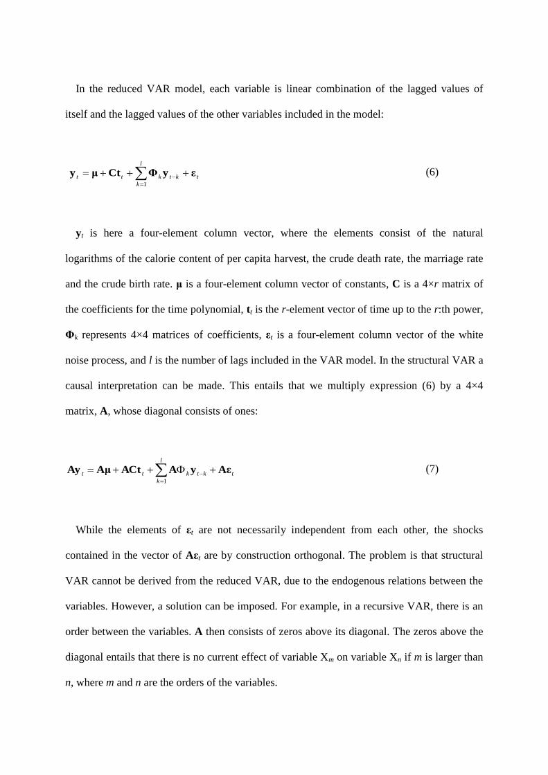
In the reduced VAR model, each variable is linear combination of the lagged values of
itself and the lagged values of the other variables included in the model:
t
l
k
ktktt εyΦCtμy
1
(6)
yt is here a four-element column vector, where the elements consist of the natural
logarithms of the calorie content of per capita harvest, the crude death rate, the marriage rate
and the crude birth rate. μ is a four-element column vector of constants, C is a 4×r matrix of
the coefficients for the time polynomial, tt is the r-element vector of time up to the r:th power,
Φk represents 4×4 matrices of coefficients, εt is a four-element column vector of the white
noise process, and l is the number of lags included in the VAR model. In the structural VAR a
causal interpretation can be made. This entails that we multiply expression (6) by a 4×4
matrix, A, whose diagonal consists of ones:
t
l
k
ktktt AεyAACtAμAy
1
(7)
While the elements of εt are not necessarily independent from each other, the shocks
contained in the vector of Aεt are by construction orthogonal. The problem is that structural
VAR cannot be derived from the reduced VAR, due to the endogenous relations between the
variables. However, a solution can be imposed. For example, in a recursive VAR, there is an
order between the variables. A then consists of zeros above its diagonal. The zeros above the
diagonal entails that there is no current effect of variable Xm on variable Xn if m is larger than
n, where m and n are the orders of the variables.

Aεt in equation (7) can also be written as Bvt, where vt is the vector of orthogonalised
shocks, while E[vtvt’] is the identity matrix, I. B is a diagonal matrix. Therefore, the vector
Bvt is also orthogonalised.
Impulse response functions and cumulative impulse response functions are a way to
graphically illustrate the impact of one variable on another over several periods. The
structural impulse response function also lends support for causal analysis.
In this study, the following causal order is assumed: harvests, crude death rates, marriage
rates and crude birth rates. Harvests should have been causally prior to any of the other three
variables. High death rates were often followed by higher marriage rates within a shorter time
span than one year. Marriage rates in the beginning of the year most likely affected birth rates
at the end of the same year.
The first step is to assess the number of lags in the VAR, which can be derived from
various information criteria. The appropriate lag order is always difficult to set. Two trend
specifications are investigated. In the specification with a quintic time polynomial, HQIC and
SBIC indicate than only one lag should be included. However, FPE and AIC indicates three
lags. For the filtered series the information criteria yield the same result.
The next step is to perform various diagnostic tests on the underlying VAR model. Testing
for the stability, shows that all eigenvalues of the companion matrix lie within the unit circle,
irrespectively of whether the underlying VAR model contains one or three lags. The stability
condition is met also when no trend is assumed. Unfortunately, the Lagrange-multiplier test
shows that the null hypothesis of no first-order residual autocorrelation is rejected at a one
percent level, whichever specification is used (see Table 5). Therefore, there could be a
misspecification in the model. The problem lies in the assumption of no structural change
during the whole period 1630–1870.
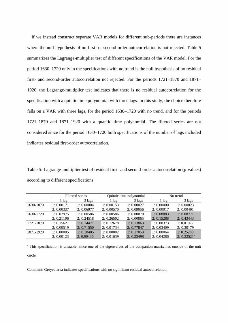
If we instead construct separate VAR models for different sub-periods there are instances
where the null hypothesis of no first- or second-order autocorrelation is not rejected. Table 5
summarizes the Lagrange-multiplier test of different specifications of the VAR model. For the
period 1630–1720 only in the specifications with no trend is the null hypothesis of no residual
first- and second-order autocorrelation not rejected. For the periods 1721–1870 and 1871–
1920, the Lagrange-multiplier test indicates that there is no residual autocorrelation for the
specification with a quintic time polynomial with three lags. In this study, the choice therefore
falls on a VAR with three lags, for the period 1630–1720 with no trend, and for the periods
1721–1870 and 1871–1920 with a quantic time polynomial. The filtered series are not
considered since for the period 1630–1720 both specifications of the number of lags included
indicates residual first-order autocorrelation.
Table 5: Lagrange-multiplier test of residual first- and second-order autocorrelation (p-values)
according to different specifications.
Filtered series Quintic time polynomial No trend
1 lag 3 lags 1 lag 3 lags 1 lag 3 lags
1630-1870 1: 0.00171
2: 0.00337
1: 0.00004
2: 0.06977
1: 0.00153
2: 0.00570
1: 0.00027
2: 0.09056
1: 0.00000
2: 0.00017
1: 0.00823
2: 0.00491
1630-1720 1: 0.02975
2: 0.21196
1: 0.00586
2: 0.24518
1: 0.00586
2: 0.26502
1: 0.00070
2: 0.00865
1: 0.08883
2: 0.15288
1: 0.08771
2: 0.43443
1721-1870 1: 0.15621
2: 0.00519
1: 0.14471
2: 0.71550
1: 0.12678
2: 0.01734
1: 0.13863
2: 0.77847
1: 0.00373
2: 0.03409
1: 0.01977
2: 0.30179
1871-1920 1: 0.00005
2: 0.00123
1: 0.18405
2: 0.90436
1: 0.00002
2: 0.01639
1: 0.17053
2: 0.23498
1: 0.00064
2: 0.04286
1: 0.25289
2: 0.22521a
a This specificiation is unstable, since one of the eigenvalues of the companion matrix lies outside of the unit
circle.
Comment: Greyed area indicates specifications with no significant residual autocorrelation.
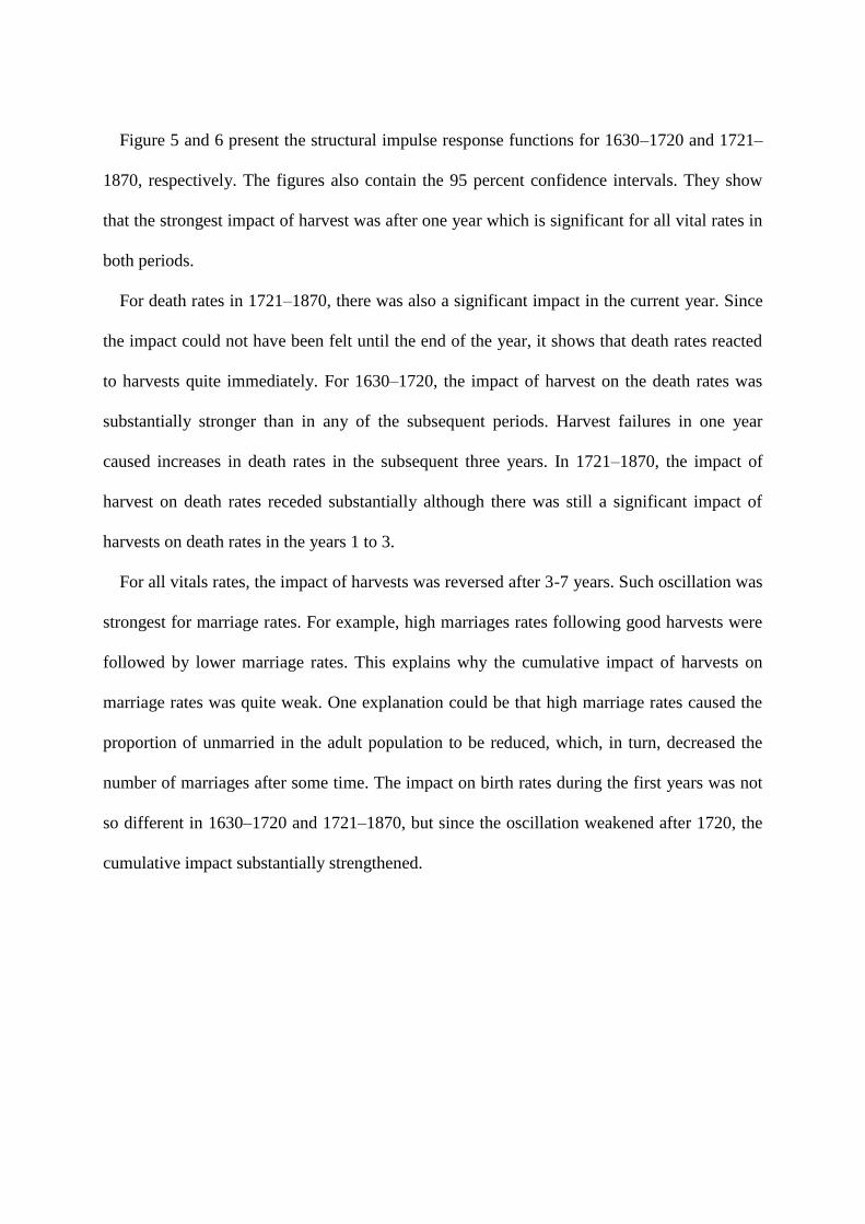
Figure 5 and 6 present the structural impulse response functions for 1630–1720 and 1721–
1870, respectively. The figures also contain the 95 percent confidence intervals. They show
that the strongest impact of harvest was after one year which is significant for all vital rates in
both periods.
For death rates in 1721–1870, there was also a significant impact in the current year. Since
the impact could not have been felt until the end of the year, it shows that death rates reacted
to harvests quite immediately. For 1630–1720, the impact of harvest on the death rates was
substantially stronger than in any of the subsequent periods. Harvest failures in one year
caused increases in death rates in the subsequent three years. In 1721–1870, the impact of
harvest on death rates receded substantially although there was still a significant impact of
harvests on death rates in the years 1 to 3.
For all vitals rates, the impact of harvests was reversed after 3-7 years. Such oscillation was
strongest for marriage rates. For example, high marriages rates following good harvests were
followed by lower marriage rates. This explains why the cumulative impact of harvests on
marriage rates was quite weak. One explanation could be that high marriage rates caused the
proportion of unmarried in the adult population to be reduced, which, in turn, decreased the
number of marriages after some time. The impact on birth rates during the first years was not
so different in 1630–1720 and 1721–1870, but since the oscillation weakened after 1720, the
cumulative impact substantially strengthened.

Figure 5: The estimated structural impulse response function, with harvests as the impulse, for
the period 1630–1720 (vertical scale – logarithms, horizontal scale – years).
-1
-0.8
-0.6
-0.4
-0.2
0
0.2
0.4
0 1 2 3 4 5 6 7 8
Response: CDR
Lower 95 percentconfidence intervalUpper 95 percentconfidence interval
-0.4
-0.3
-0.2
-0.1
0
0.1
0.2
0.3
0.4
0.5
0.6
0 1 2 3 4 5 6 7 8
Response: MR
Lower 95 percentconfidence intervalUpper 95 percentconfidence interval
-0.4
-0.3
-0.2
-0.1
0
0.1
0.2
0.3
0.4
0.5
0.6
0 1 2 3 4 5 6 7 8
Response: CBR
Lower 95 percentconfidence intervalUpper 95 percentconfidence interval

Figure 6: The estimated structural impulse response function, with harvests as the impulse, for
the period 1721–1870 (vertical scale – logarithms, horizontal scale – years).
-1
-0.8
-0.6
-0.4
-0.2
0
0.2
0.4
0 1 2 3 4 5 6 7 8
Response: CDR
Lower 95 percentconfidence intervalUpper 95 percentconfidence interval
-0.4
-0.3
-0.2
-0.1
0
0.1
0.2
0.3
0.4
0.5
0.6
0 1 2 3 4 5 6 7 8
Response: MR
Lower 95 percentconfidence intervalUpper 95 percentconfidence interval
-0.4
-0.3
-0.2
-0.1
0
0.1
0.2
0.3
0.4
0.5
0.6
0 1 2 3 4 5 6 7 8
Response: CBR
Lower 95 percentconfidence intervalUpper 95 percentconfidence interval
The cumulative structural impulse response function (csirf) is not the same as the
cumulative elasticity with harvest as the impulse. The former is the cumulative response of a
one-unit shock of harvest on vital rates. However, part of the effect is through changing
harvest in the next periods. For example, if a one-unit increase in harvest causes harvest also
to increase by half a unit the next year, this also adds to the impact on the vital rates.
Therefore a one-unit increase in the harvest the current year is, in this example, a de facto
one-and-a-half unit increase in the harvests accumulated during the whole period. To estimate
the cumulative elasticity of vital rates with respect to harvest, we have to divide the csirf with

harvest as impulse and a vital rate as the response with the csirf with harvest as both impulse
and response. Table 5 displays the estimates.
The cumulative structural impulse response function with harvest as impulse and response
declined quite dramatically, from 1.85 in 1630–1720 to unity in 1721–1870. Before 1630
chocks to harvests in one year had strong repercussions on later harvests, while after 1720 this
was no longer the case. For the period 1630–1720 the decline substantially reduces the
estimated cumulative elasticity of vital rates when compared to the cumulative structural
impulse response function.
For death rates in 1630–1720, the estimated cumulative elasticity in Table 5, at -1.3, is
somewhat weaker than according to the distributed lag model. However, the change in 1720
was not as dramatic as according to the DLM, and there was a slight weakening after 1870,
contrary to the result in Table 2.
Table 6 shows that for both marriage and birth rates, the cumulative elasticities
significantly strengthened after 1720, while they disappeared after 1870. However, despite the
significant impact after one year, the cumulative elasticity of marriage rates was not
significant in any of the investigated periods. The cumulative elasticity of birth rates was at
0.6 in 1721–1870, which was stronger than according to the DLM, while it was not significant
in any of the other sub-periods.
Overall Table 6 yields a similar picture as for the DLM: while after 1720 positive checks
weakened, preventive checks strengthened, and while after 1870 preventive checks
disappeared, positive checks continued to exist until 1920.
[Insert Table 6 here]
5. Putting the empirical findings in context
There are several possible explanations for the decline in the elasticity of the crude death rate
in Sweden after the 1710s. In particular, the years around 1650–1720 experienced severe
economic difficulties. It took time for the economy to recover.28
Climatic factors might also
be important. A reconstruction of winter temperatures for Stockholm shows that a previous
cold period beginning in the mid-sixteenth century ended around 1700 and that the 1730s was
an unusually warm decade.29
Other explanations for the decreased occurrence of severe
mortality crises in Europe during the eighteenth century include a mutual adaptation between
pathogen and host that decreased mortality levels during plagues, improved private and public
hygiene and an enhanced system of transportation and market integration.30
The result of the present study that preventive checks disappeared after 1870 accords quite
well with the description by Dribe of the fertility pattern in Sweden before 1880 as natural.31
Bengtsson and Dribe find that in Scania there was a strong fertility response to changes in
food prices during the whole period 1766–1864.32
The strong support for the existence of positive and preventive checks up to the nineteenth
century can be contrasted to earlier research on England. Using VAR methods, Nicolini finds
that the negative effect of real wages on mortality rates in England was significant only up to
1640, while the positive effect on fertility was significant only up to 1740.33
Crafts and Mills
cannot find any evidence of positive checks even for the period 1542–1645 and conclude that
28 Morell (1986), pp. 260–261.
29 Leijonhufvud et al. (2001).
30 Livi-Bacci (2007), p. 67.
31 Dribe (2008).
32 Bengtsson and Dribe (2006).
33 Nicolini (2007).

preventive checks disappeared by the early seventeenth century.34
Recently, Rathnke and
Sarferaz question this result, contending that by using a time-varying VAR model preventive
and positive checks are made visible in the English data up to the nineteenth century.35
A
problem with all of these studies, and a clear disadvantage to the present study, is that they
use real wage as an indicator for living standards.
England was most likely earlier in its transition to a post- or late Malthusian economy.
Compared with England,36
the spikes in Swedish mortality rates up to the early eighteenth
century were at a much higher level (see Figure 1). France displayed a similar development as
that in Sweden, with a marked decline in severe mortality crises during the course of the
eighteenth century, while in other European countries the decline was more protracted and
came later.37
Nevertheless, as for Sweden, it is likely that other results could be found for
England if elasticities were computed with respect to harvest or food production or if the
series of crude death rate for England is upgraded during mortality peaks in light of the
criticism directed against the demographic reconstruction of Wrigley and Schofield.
The decline in the sensitivity of mortality after 1720 may be surprising given that earlier
Swedish studies show that there was a very strong dependency on cereal products in the
eighteenth century, while animal products stood for only a small part of the diet.38
However,
per capita food consumption did not decline during the course of the seventeenth and
eighteenth centuries, while GDP per capita increased somewhat despite the relatively fast
population growth.39
The significant growth in the size of the population during the eighteenth
34 Crafts and Mills (2009), p. 80.
35 Rathnke and Sarferaz (2010).
36 Wrigley and Schofield (1989), pp. 531–535.
37 Livi-Bacci (2007), p. 67.
38 Morell (1986).
39 Edvinsson (2013a).
century was in itself a manifestation of a dynamic economy. Gadd describes Sweden as going
through an agrarian revolution in the eighteenth and nineteenth centuries.40
Import of grains
also dampened the impact of harvest fluctuations on death rates.
For Germany, Pfister and Fertig find that positive checks substantially weakened after the
1810s,41
which is not as visible in the Swedish material. The present study reproduces the
result by Galloway that there were strong positive checks in Sweden after the industrial
breakthrough and that positive checks were not attenuated over time (which he also argues
was the case for France).42
It was only after 1920, that the positive checks disappeared, while
the structural VAR analysis indicates that some attenuation may have occurred after 1870.
To some extent, the response of the marriage rate is a more direct indicator of preventive
checks, since some of the responses of birth rates, at least in the short-term, reflected changed
nutritional standards rather than active preventive behaviour. The present study indicates that
the elasticity of the marriage rate displayed a similar trend as the elasticity of the birth rate.
The very weak, and insignificant, elasticity of the marriage rate in 1630–1720 supports the
view that there was a hidden demographic transition between the seventeenth and eighteenth
centuries as argued by some Swedish historians. Higher death rates tended to increase the
number of marriages. Lower life span induced a lower age at marriage. When the mortality
crises attenuated after the 1710s, preventive checks became more predominant.
6. Conclusions
Malthus’ original formulation of his model of preventive and positive checks related vital
rates to the production of land, not without good reason. The present study argues that one of
40 Gadd (2000).
41 Pfister and Fertig (2010), p. 48.
42 Galloway (1994), p. 24.
the most important indicators used by present-day Malthusians – real wage – could be
problematic when analysing the Malthusian world. Instead, this study investigates the short-
term Malthusian mechanism by using a series of harvests transformed into the production of
per capita calories.
The present study uses different models to estimate the cumulative elasticities of vital rates:
DLM, ARMAX and SVAR. In addition, various specifications are used concerning the
underlying trends and the number of lags included. The main result is, however, robust to the
specifications made. All models support the weaker version of the Malthusian model. In the
pre-industrial Sweden, there was a short-term Malthusian mechanism in terms of strong
positive and preventive checks, without that implying that per capita income declined due to
population growth. Through the effect on death and birth rates, natural population growth was
strongly affected by harvest fluctuations. The impact of harvests on various demographic
indicators was stretched over several years. The strongest impact was from the harvests
lagged by one and two years. All major spikes in death rates were preceded by one or two
years of harvest failures. An important finding is that structural breaks occurred around 1720
and 1870.
In line with the finding of Galloway for France and Sweden, the present study finds that
positive checks existed up to 1920.43
In 1630–1720, the cumulative elasticity of the crude
death rate was stronger than in any subsequent period according to all the specifications used
in this study, reflecting the mortality crises occurring in this period. Up to the early eighteenth
century, the cumulative elasticity of death rates was much stronger than of birth and marriage
rates. A fundamental change occurred after 1720. Preventive checks were initially
strengthened, while they disappeared after the rise of the industrial society in the final decades
43 Galloway (1994).
of the nineteenth century, in accordance with earlier findings by Swedish researchers on
changing fertility patterns. This development also accords quite well with the prediction of the
unified growth theory that in the initial phase of technological acceleration (which Swedish
agriculture experienced in the eighteenth century) preventive checks strengthened, while
positive checks attenuated. However, to what extent there was a long-term adjustment of vital
rates and population growth to harvest output need further investigation.
The demographic transition implied that first death rates went down, but not birth rates,
which accelerated population growth. Second, birth rates also declined, which completed the
transition.44
Even if the lower floor of the crude death rate did not start to decline until the
1820s and 1830s (see Figure 1), the transformation in the elasticity of death rates a century
earlier was critical.
This paper shows that the Swedish economy in the seventeenth century deviated from that
of the English economy. According to the data of Wrigley and Schofield England had already
embarked on a similar transformation much earlier than Sweden. Based on English data,
Nicoloni concludes that ‘perhaps the world before Malthus was not so Malthusian’.45
Early
modern Swedish data can probably better illuminate the dynamics of the agrarian economy,
given the special features of England as the first country experiencing an industrial revolution.
Furthermore, the reliability of the English data has been questioned. Even if England has a
continuous series of vital rates that goes further back in time than for any other country, the
reliability of the Swedish data is superior for the second half of the eighteenth century to any
other country due to the early official statistics.
44 Lee and Anderson (2002).
45 Nicoloni (2007).

Data appendix
Data on population, mortality, fertility and nuptility is from a previous study.46
These series
are based on data from Palm and Heckscher.47
For the eighteenth century Palm most likely
underestimates the size of population and the vital rates. For 1630 the population within the
borders of Sweden is raised from 0.912 to 1.12 million, while for 1700 it is raised from 1.373
to 1.44 million compared to Palm. The trends in vital rates and total population are
substantially revised, while annual fluctuations closely follow the data of Palm. From the mid-
eighteenth century the population data is from Statistics Sweden.48
The series of per capita harvest is from previous published studies of the author.49
Krantz
and Schön present an alternative agricultural series for the early modern period based on the
so-called demand approach, but it does not distinguish between harvests and animal
products.50
From 1802, the harvests are derived from reports on the yield ratios (gross
harvests divided by seed) of different grains for all Swedish 24 counties. The absolute levels
of harvests are uncertain for the nineteenth century, but annual fluctuations are of high
reliability due to the detailed make-up of the primary material. For the period before 1802, the
harvest series is constructed from three indicators: tithes, subjective harvest estimates and
grain prices. Grain prices are not a direct indicator of harvest fluctuations. Nevertheless, in a
previous study by the author it is shown that for the early nineteenth century a regression
model where grain prices for two consecutive years are included as independent variables,
together with another indicator of harvests, can explain over 85 per cent of the variance in
46 Edvinsson (2015).
47 Palm (2000 and 2001); Heckscher (1936).
48 Statistics Sweden (1999).
49 Edvinsson (2009, 2013a, and 2013b).
50 Krantz and Schön (2012).

annual harvest fluctuations. It is only for later periods that grain prices were weakly related to
harvests.51
For the period from 1802 gross harvests are transformed into calories. One kilogram of
wheat is assumed to contain 3365 kcal, one kilogram of rye 3433 kcal, one kilogram of barley
3404 kcal, one kilogram of oats 3369 kcal, one kilogram of dredge 3387 kcal, one kilogram of
peas, beans, or vetch 3285 kcal, one kilogram of potatoes 670 kcal, one kilogram of sugar
beets 430 kcal, one kilogram of oil plants 2700 kcal, and one kilogram of triticale 3399 kcal.
Before 1802 the calorie content of harvests are assumed to follow their volume growth.
The wage series (in Figure 4) is spliced from three series, where the nominal wage is
deflated by the Consumer Price Index:52
for 1630–1732, the day rate of male manual labour in
Stockholm;53
for 1732–1914, the day rate of male agrarian labour in the whole country;54
and
from 1914, the hourly wage of male workers in industry.55
The standard deviations of the first
and third series are adjusted to conform to the standard deviation of the series of 1732–1914,
by using the ratios of standard deviations in annual logarithmic changes for overlapping
periods.
For 1732–1913, grain prices (in Figure 4) are based on the average national price of various
grains56
using quantity weights from the early twentieth century. For the period 1913–1949,
the quantity weights are from 1913. For the period before 1732, the series is mostly based on
51 Edvinsson (2009).
52 Author and co-author, published study from 2011.
53 Söderberg (2010).
54 Jörberg (1972), vol. 2.
55 Prado (2010).
56 Jörberg (1972), vol. 2.

the prices of rye and barley.57
The nominal price is transformed to being expressed in grams
of gold.
References
Allen, R., ‘The Great Divergence in European Wages and Prices from the Middle Ages to the
First World War’, Explorations in Economic History 38 (2001), pp. 411–447.
Åmark, K., Spannmålshandel och spannmålspolitik i Sverige 1719–1830 (Stockholm, 1915).
Bengtsson, T., ‘Living standards and economic stress’, in T. Bentsson, Campbell, C, and Lee
J. Z, (eds.), Life under Pressure. Mortality and Living Standards in Europe and Asia,
1700–1900 (Cambridge, MA, 2004), pp. 27–59.
Bengtsson, T. and Dribe, M., ‘Deliberate control in natural fertility population: Southern
Sweden, 1766–1864’, Demography 43 (2006), pp. 727–746.
Bengtsson, T. and Broström, G., ‘Famines and mortality crises in 18th to 19th century
southern Sweden’, GENUS LXVII (2011), pp. 119–139.
Bengtsson, T. and Oeppen, J., ‘A reconstruction of the population of Scania 1650–1760’,
Lund papers in economic history, no. 32 (1993).
Bengtsson, T. and Ohlsson, R., ‘Age-Specific Mortality and short-term changes in the
standard of living: Sweden, 1751–1859’, European Journal of Population 1 (1985), pp.
309–326.
Chiarini, B., ‘Was Malthus right? The relationship between population and real wages in
Italian history, 1320 to 1870’, Explorations in Economic History 47 (2010), pp. 460–475.
57 Edvinsson (2012).
Clark, G., A Farewell to Alms: A Brief Economic History of the World (Princeton and Oxford,
2007).
Crafts, N., Mills, T., ‘From Malthus to Solow: How did the Malthusian economy really
evolve’, Journal of Macroeconomics 31 (2009), pp. 68–93.
Dribe, M., ‘Dealing with economic stress through migration: Lessons from nineteenth century
rural Sweden’, European Review of Economic History 7 (2003), pp. 271–299.
Dribe, M., ‘Demand and supply factors in the fertility transition: a county-level analysis of
age-specific marital fertility in Sweden, 1880–1930’, European Review of Economic
History 13 (2008), pp. 65–94.
Dribe, M., Olsson, M. and Svensson, P., ‘Production, prices and mortality: Demographic
response to economic hardship in rural Sweden 1750–1860’. Unpublished paper,
presented at the European Historical Economics Society (Dublin, 2011).
Eckstein, Z., Schultz, T. P. and Wolpin, K. I., ‘Short-run fluctuations in fertility and mortality
in pre-industrial Sweden’, European Economic Review 26 (1984), pp. 295–317.
Edvinsson, R., ‘Swedish harvests 1665-1820: Early modern growth in the periphery of
European economy’, Scandinavian Economic History Review 57 (2009), pp. 2-25.
Edvinsson, R., ‘Harvests and grain prices in Sweden 1665-1870’, Agricultural History Review
60 (2012), pp. 1-18.
Edvinsson, R., ‘New Annual Estimates of Swedish GDP in 1800-2010’, The Economic
History Review 66 (2013), pp. 1101–1126.
Edvinsson, R., ‘Swedish GDP 1620-1800: Stagnation or Growth?’, Cliometrica 7 (2013), pp.
37-60.

Edvinsson, R., ‘Recalculating Swedish pre-census demographic data: Was there acceleration
in early modern population growth?’, Cliometrica 9, 2015, pp. 167-191.
Edvinsson, R., and Söderberg, J., ‘A Consumer Price Index for Sweden 1290-2008’, Review
of Income and Wealth 57 ( 2011), pp. 270-292.
Gadd, C.-J., Den agrara revolutionen 1700–1870, (Stockholm, 2000).
Galloway, P. R., ‘Basic patterns in annual variations in fertility, nuptiality, mortality and
prices in pre-industrial Europe’, Population Studies – A Journal of Demography 42
(1988), pp. 275–303.
Galloway, P. R., ‘A Reconstruction of the Population of North Italy from 1650 to 1881 using
Annual Inverse Projection with Comparisons to England, France, and Sweden’, European
Journal of Population 10 (1994), pp. 223–274.
Galloway, P. R., ‘Secular changes in the short-term preventive, positive, and temperature
checks to population growth in Europe, 1460 to 1909’, Climatic Change 26 (1994), pp. 3–
63.
Galor, O. and Weil, D. N., ‘Population, Technology, and Growth: From Malthusian
Stagnation to the Demographic Transition and Beyond’, American Economic Review 90
(2000), pp. 806–828.
Heckscher, E., Sveriges ekonomiska historia från Gustav Vasa, vol. I:1–I:2 (Stockholm
(1935–1936).
Heckscher, E., Ekonomisk-historiska studier (Stockholm, 1936).
Hillingsworth, T. H., Historical Demography (London and Southampton, 1969).
Hoffman, P., ‘Land Rents and Agricultural Productivity: The Paris Basin, 1450–1789’,
Journal of Economic History 51 (1991), pp. 771–805.
Jörberg, L., A History of Prices in Sweden 1732–1914 (Lund, 1972).

Klemp, M., and Møller, N. F., ‘Post-Malthusian Dynamics in Pre-Industrial Scandinavia’,
Discussion Papers No. 15-03 (2015), Department of Economics, University of
Copenhagen.
Krantz, O. and Schön, L., ‘The Swedish economy in the early modern period: constructing
historical national accounts’, European Review of Economic History 16 (2012), pp. 529–
549.
Larsen, U., ‘Determinants of short-term fluctuations in nuptiality in Sweden, 1751–1913:
Application of Multivariate ARIMA Models’, European Journal of Population 3 (1987),
pp. 203–232.
Larsson, D., Den dolda transitionen: Om ett demografiskt brytningsskede i det tidiga 1700-
talets Sverige (Gothenburg, 2006).
Lee, R., ‘The demographic transition: three centuries of fundamental change’, Journal of
Economic Perspectives 17 (2003), pp. 167–90.
Lee, R. and Anderson, M., ‘Malthus in state space: Macro economic-demographic relations in
English history, 1540 to 1870’, Journal of Population Economics 15 (2002), pp. 195–220.
Leijonhufvud, L., Grain Tithes and Manorial Yields in Early Modern Sweden: Trends and
patterns of production and productivity c. 1540–1680 (Uppsala, 2001).
Leijonhufvud, L., Wilson, R., Moberg, A., Söderberg, J., Retsö, D. and Söderlind, U., ‘Five
centuries of Stockholm winter/spring temperatures reconstructed from documentary
evidence and instrumental observations’, Climatic Change 101 (2010), pp. 109–141.
Livi-Bacci, M., A Concise History of World Population (Cambridge, Mass., 2007).
Maddison, A., Contours of the World Economy, 1–2030 AD: Essays in Macro-Economic
History (Oxford, 2007).
Malthus, T., An Essay on the Principles of Population (London, 1985).
McKeown, T., The Modern Rise of Population (London, 1976).

Mokyr, J. and Voth, H.-J., ‘Understanding growth in Europe, 1700–1870: theory and
evidence’, in S. Broadberry and K. O’Rourke, K., eds., The Cambridge Economic History
of Modern Europe, vol. 1 (Cambridge, 2008), pp. 4–42
Møller, N. F., Sharp, P., ‘Malthus in cointegration space: evidence of a post-Malthusian pre-
industrial England’, Journal of Economic Growth 19 (2014), pp. 105–140.
Morell, M., Eli F. Heckscher, utspisningsstaterna och den svenska livsmedelskonsumtionen
från 1500-talet till 1800-talet: Sammanfattning och komplettering av en lång debatt
(Uppsala, 1986).
Morell, M., Studier i den svenska livsmedelskonsumtionens historia: Hospitalhjonens
livsmedelskonsumtion 1621–1872 (Uppsala, 1989).
Myrdal, J., Jordbruket under feodalismen: 1000–1700 (Lagersberg, 1999).
Nelson, M., Bitter Bread: The Famine in Norrbotten 1867–1868 (Uppsala, 1988).
Nicolini, E., ‘Was Malthus right? A VAR analysis of economic and demographic interactions
in pre-industrial England’, European Review of Economic History 11 (2007), pp. 99–121.
Ó Gráda, C., ‘Markets and Famines: Evidence from Nineteenth‐Century Finland’, Economic
Development and Cultural Change 49 (2001), pp. 575–590.
Oeppen, J., ‘Back Projection and Inverse Projection: Members of a Wider Class of
Constrained Projection Models’, Population Studies – A Journal of Demography 47
(1993), pp. 245–267.
Palm, L. A., Folkmängden i Sveriges socknar och kommuner 1571–1997: Med särskild
hänsyn till perioden 1571–1751 (Gothenburg, 2000)
Palm, L. A., Livet, kärleken och döden: Fyra uppsatser om svensk befolkningsutveckling
1300–1850 (Gothenburg, 2001).
Persson, K.-G., ‘The Malthus Delusion’, European Review of Economic History 12 (2008),
pp. 165–173.
Pfister, U., Fertig, G., ‘The Population History of Germany: Research Strategy and
Preliminary Results’, MPIDR Working Paper WP 2010-035 (2010).
Prado, S., ‘Nominal and real wages of manufacturing workers, 1860–2007’, in R. Edvinsson,
T. Jacobson and D. Waldenström, eds, Historical Monetary and Financial Statistics for
Sweden: Exchange rates, prices and wages 1277–2008 (Stockholm, 2010), pp. 479–527.
Rathke, A. and Sarferaz, S., ‘Malthus Was Right: New Evidence from a Time-Varying VAR’.
Institute for Empirical Research in Economics, University of Zurich, Working Paper No.
477 (2010).
Razzel, P., ‘The Growth of Population in Eighteenth-Century England: A Critical
Reappraisal’, Journal of Economic History 53 (1993), pp. 743–771.
Statistics Sweden, Population development in Sweden in a 250-year perspective (Stockholm,
1999).
Sundquist, S., Sveriges folkmängd på Gustaf II Adolfs tid: En demografisk studie (Lund,
1938).
Söderberg, J., ‘Real wage trends in urban Europe, 1730–1850: Stockholm in a comparative
perspective’, Social History 12 (1987), pp. 155–176.
Söderberg, J., ‘Long-term trends in real wages of labourers’, in R. Edvinsson, T. Jacobson and
D. Waldenström, eds, Historical Monetary and Financial Statistics for Sweden: Exchange
rates, prices and wages 1277–2008 (Stockholm, 2010), pp. 453–478.

Voigtländer N., Voth, H.-J., ‘Malthusian Dynamism and the Rise of Europe: Make War, Not
Love’, American Economic Review 99 (2009), pp. 248–254.
Willner, S., ‘Hälso- och samhällsutvecklingen i Sverige 1750–2000’, in J. Sundin, C.
Hogstedt. J. Lindberg and H. Moberg, eds., Svenska folkets hälsa i historiskt perspektiv.
Statens folkhälsoinstitut (Stockholm, 2005), pp. 35–80.
Wrigley, E. A. and Schofield, R., The Population History of England 1541–1871: A
reconstruction, paperback ed. (Cambridge, 1989).