PRE-LAB PREPARATION SHEET FOR LAB 2: CHANGING MOTION (Due at the beginning of Lab 2) Directions: Read over Lab 2 and then answer the following questions about the procedures. 1. In Activity 1-1, how do you expect that your position–time graph will differ from

those you observed in Lab 1, where you were moving with a constant velocity? 2. Show how you would add the two vectors shown below:

3. Show below how you would subtract the second vector from the first.

4. In words, write down definitions for average velocity and instantaneous velocity. 5. What do you predict the direction (sign) of acceleration will be for the experiment in

Activity 3-2: Speeding Up Toward the Motion Detector?

LAB 2: CHANGING MOTION

A cheetah can accelerate from 0 to 50 miles per hour in 6.4 seconds. —Encyclopedia of the Animal World A Jaguar can accelerate from 0 to 50 miles per hour in 6.1 seconds. —World Cars OBJECTIVES

• To discover how and when objects accelerate. • To understand the meaning of acceleration, its magnitude, and its direction. • To discover the relationship between velocity and acceleration graphs. • To learn how to represent velocity and acceleration using vectors. • To learn how to find average acceleration from acceleration graphs. • To learn how to calculate average acceleration from velocity graphs.

OVERVIEW In the previous lab, you looked at position–time and velocity–time graphs of the motion of your body and a cart at a constant velocity. You also looked at the acceleration–time graph of the cart. The data for the graphs were collected using a motion detector. Your goal in this lab is to learn how to describe various kinds of motion in more detail. You have probably realized that a velocity–time graph is easier to use than a position–time graph when you want to know how fast and in what direction you are moving at each instant in time as you walk (even though you can calculate this information from a position–time graph). It is not enough when studying motion in physics to simply say that “the object is moving toward the right” or “it is standing still.” When the velocity of an object is changing, it is also important to describe how it is changing. The rate of change of velocity with respect to time is known as the acceleration. To get a feeling for acceleration, it is helpful to create and learn to interpret velocity–time and acceleration–time graphs for some relatively simple motions of a cart on a smooth

ramp or other level surface. You will be observing the cart with the motion detector as it moves with its velocity changing at a constant rate. INVESTIGATION 1: VELOCITY AND ACCELERATION GRAPHS In this investigation you will be asked to predict and observe the shapes of velocity–time and acceleration–time graphs of a cart moving along a smooth ramp or other level surface. You will focus on cart motions with a steadily increasing velocity. You will need the following materials:

• computer-based laboratory system • motion detector • RealTime Physics Mechanics experiment configuration files • cart with very little friction • smooth ramp or other level surface 2–3 m long • fan unit attachment with batteries and dummy cells (or with a speed adjustment

control) Activity 1-1: Speeding Up

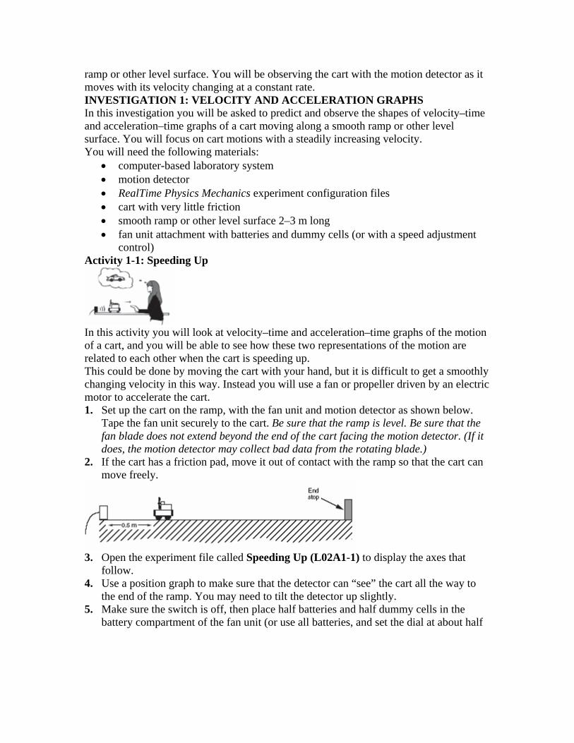
In this activity you will look at velocity–time and acceleration–time graphs of the motion of a cart, and you will be able to see how these two representations of the motion are related to each other when the cart is speeding up. This could be done by moving the cart with your hand, but it is difficult to get a smoothly changing velocity in this way. Instead you will use a fan or propeller driven by an electric motor to accelerate the cart. 1. Set up the cart on the ramp, with the fan unit and motion detector as shown below.

Tape the fan unit securely to the cart. Be sure that the ramp is level. Be sure that the fan blade does not extend beyond the end of the cart facing the motion detector. (If it does, the motion detector may collect bad data from the rotating blade.)

2. If the cart has a friction pad, move it out of contact with the ramp so that the cart can move freely.

3. Open the experiment file called Speeding Up (L02A1-1) to display the axes that

follow. 4. Use a position graph to make sure that the detector can “see” the cart all the way to

the end of the ramp. You may need to tilt the detector up slightly. 5. Make sure the switch is off, then place half batteries and half dummy cells in the

battery compartment of the fan unit (or use all batteries, and set the dial at about half

maximum speed of the fan blade). To preserve the batteries, switch on the fan unit only when you are making measurements.

6. Hold the cart with your hand on its side, begin graphing, switch the fan unit on and when you hear the clicks of the motion detector, release the cart from rest. Do not put your hand between the cart and the detector. Be sure to stop the cart before it hits the end stop. Turn off the fan unit. Repeat, if necessary, until you get a nice set of graphs. Adjust the position and velocity axes if necessary so that the graphs fill the axes. Use the features of your software to transfer your data so that the graphs will remain persistently displayed on the screen. Also save your data for analysis in Investigation 2. (Name your file SPEEDUP1.XXX, where XXX are your initials.)

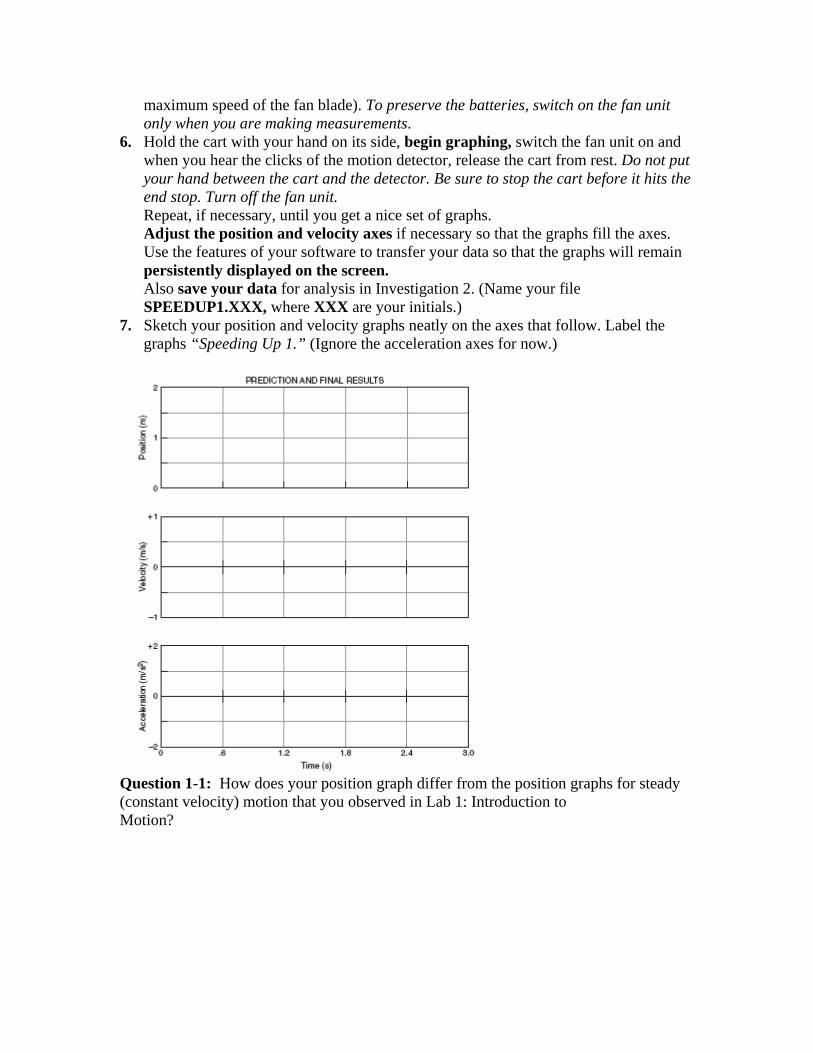
7. Sketch your position and velocity graphs neatly on the axes that follow. Label the graphs “Speeding Up 1.” (Ignore the acceleration axes for now.)

Question 1-1: How does your position graph differ from the position graphs for steady (constant velocity) motion that you observed in Lab 1: Introduction to Motion?

Question 1-2: What feature of your velocity graph signifies that the motion was away from the motion detector? Question 1-3: What feature of your velocity graph signifies that the cart was speeding up? How would a graph of motion with a constant velocity differ? 8. Adjust the acceleration scale so that your graph fills the axes. Sketch your graph on

the acceleration axes above, and label it “Speeding Up 1.”

Question 1-4: During the time that the cart is speeding up, is the acceleration positive or negative? How does speeding up while moving away from the detector result in this sign of acceleration? (Hint: Remember that acceleration is the rate of change of velocity. Look at how the velocity is changing. It takes two points on the velocity–time graph to calculate the rate of change of velocity.) Question 1-5: How does the velocity vary in time as the cart speeds up? Does it increase at a steady (constant) rate or in some other way? Question 1-6: How does the acceleration vary in time as the cart speeds up? Is this what you expect based on the velocity graph? Explain. Question 1-7: The diagram below shows the positions of a cart at equal time intervals as it speeds up. Assume that the cart is already moving at t1.

At each indicated time, sketch a vector above the cart that might represent the velocity of the cart at that time while it is moving away from the motion detector and speeding up. Question 1-8: Show below how you would find the vector representing the change in velocity between the times 2 and 3 s in the diagram above. (Hint: Remember that the change in velocity is the final velocity minus the initial velocity, and the vector difference is the same as the sum of one vector and the negative of the other vector.) Based on the

direction of this vector and the direction of the positive x axis, what is the sign of the acceleration? Does this agree with your answer to Question 1-4? Activity 1-2: Speeding Up More Prediction 1-1: Suppose that you accelerate the cart at a faster rate. How would your velocity and acceleration graphs be different? Sketch your predictions with dashed or different color lines on the previous set of axes. 1. Test your predictions. Make velocity and acceleration graphs. This time accelerate the

cart with the maximum number of batteries in the battery compartment (or set the dial to the maximum speed of the fan blade). Remember to switch the fan unit on only when making measurements. Repeat if necessary to get nice graphs. (Leave the original graphs persistently displayed on the screen.) When you get a nice set of graphs, save your data as SPEEDUP2.XXX for analysis in Investigation 2.

2. Sketch your velocity and acceleration graphs with solid or different color lines on the previous set of axes, or print the graphs and affix them over the axes. Be sure that the graphs are labeled “Speeding Up 1” and “Speeding Up 2.”

Question 1-9: Did the shapes of your velocity and acceleration graphs agree with your predictions? How is the magnitude (size) of acceleration represented on a velocity–time graph? Question 1-10: How is the magnitude (size) of acceleration represented on an acceleration–time graph? INVESTIGATION 2: MEASURING ACCELERATION In this investigation you will examine the motion of a cart accelerated along a level surface by a battery driven fan more quantitatively. This analysis will be quantitative in the sense that your results will consist of numbers. You will determine the cart’s acceleration from your velocity–time graph and compare it to the acceleration read from the acceleration–time graph. You will need motion software and the data files you saved from Investigation 1. Activity 2-1: Velocity and Acceleration of a Cart That Is Speeding Up 1. The data for the cart accelerated along the ramp with half batteries and half dummy

cells (Investigation 1, Activity 1-1) should still be persistently on the screen. (If not, load the data from the file SPEEDUP1.XXX.) Display velocity and acceleration, and adjust the axes if necessary.

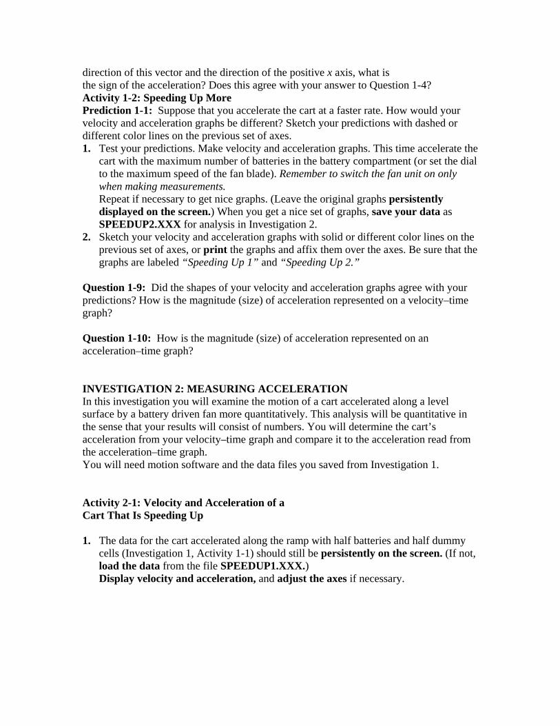
2. Sketch the velocity and acceleration graphs again below, or print, and affix a copy of the graphs. Correct the scales if necessary.

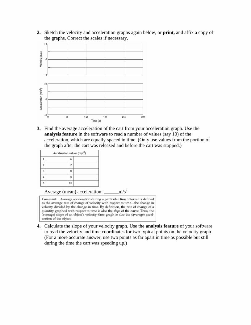
3. Find the average acceleration of the cart from your acceleration graph. Use the

analysis feature in the software to read a number of values (say 10) of the acceleration, which are equally spaced in time. (Only use values from the portion of the graph after the cart was released and before the cart was stopped.)

Average (mean) acceleration: ______m/s2

4. Calculate the slope of your velocity graph. Use the analysis feature of your software

to read the velocity and time coordinates for two typical points on the velocity graph. (For a more accurate answer, use two points as far apart in time as possible but still during the time the cart was speeding up.)

Calculate the change in velocity between points 1 and 2. Also calculate the corresponding change in time (time interval). Divide the change in velocity by the change in time. This is the average acceleration. Show your calculations below.

Question 2-1: Is the acceleration positive or negative? Is this what you expected? Question 2-2: Does the average acceleration you just calculated agree with the average acceleration you found from the acceleration graph? Do you expect them to agree? How would you account for any differences? Activity 2-2: Speeding Up More 1. Load the data from your file SPEEDUP2.XXX (Investigation 1, Activity 1-2).

Display velocity and acceleration. 2. Sketch the velocity and acceleration graphs or print and affix the graphs. Use dashed

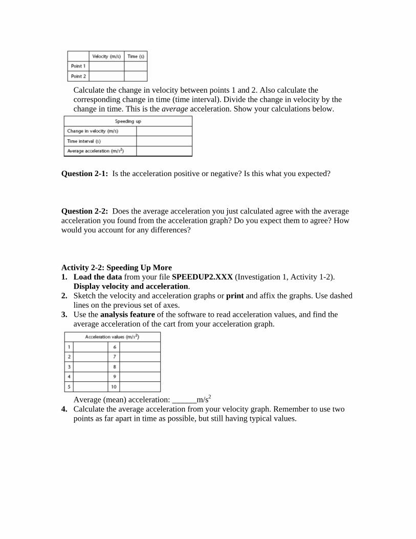
lines on the previous set of axes. 3. Use the analysis feature of the software to read acceleration values, and find the

average acceleration of the cart from your acceleration graph.

Average (mean) acceleration: ______m/s2

4. Calculate the average acceleration from your velocity graph. Remember to use two points as far apart in time as possible, but still having typical values.

Calculate the average acceleration.

Question 2-3: Does the average acceleration calculated from velocities and times agree with the average acceleration you found from the acceleration graph? How would you account for any differences? Question 2-4: Compare this average acceleration to that with half batteries and half dummy cells (Activity 2-1). Which is larger? Is this what you expected? If you have additional time, do the following Extension. Extension 2-3: Using Statistics and Fit to Find the Average Acceleration In Activity 2-1 and 2-2, you found the value of the average acceleration for a motion with steadily increasing velocity in two ways: from the average of a number of values on an acceleration–time graph and from the slope of the velocity–time graph. The statistics feature in the software allows you to find the average (mean) value directly from the acceleration–time graph. The fit routine allows you to find the line that best fits your velocity–time graph from Activity 2-1 and 2-2. The equation of this line includes a value for the slope. 1. Using Statistics: Load your SPEEDUP1.XXX file. You must first select the portion

of the acceleration–time graph for which you want to find the mean value. Next, use the statistics feature and read the mean value of acceleration from the table: ______m/s2

Question E2-5: Compare this value to the one you found from 10 measurements in Activity 2-1. 2. Using Fit: You must first select the portion of the velocity–time graph that you want

to fit. Next, use the fit routine to try a linear fit, v = b + ct.

Record the equation of the fit line, and compare the value of the slope (c) to the acceleration you found in Activity 2-1.

Question E2-6: What is the physical meaning of b? Question E2-7: How do the two values of acceleration that you found in this extension agree with each other? Is this what you expected? Find the average acceleration for the motion in your SPEEDUP2.XXX file from the acceleration–time and velocity–time graphs using the same methods. Compare the values to those found in Activity 2-2 by averaging 10 values. INVESTIGATION 3: SLOWING DOWN AND SPEEDING UP In this investigation you will look at a cart moving along a ramp or other level surface and slowing down. A car being driven down a road and brought to rest when the brakes are applied is a good example of this type of motion. Later you will examine the motion of the cart toward the motion detector and speeding up. In both cases, we are interested in how velocity and acceleration change over time. That is, we are interested in the shapes of the velocity–time and acceleration–time graphs (and their relationship to each other), as well as the vectors representing velocity and acceleration. You will need the following materials:

• computer-based laboratory system • motion detector • RealTime Physics Mechanics experiment configuration files • cart with very little friction • smooth ramp or other level surface 2–3 m long • fan unit attachment with batteries

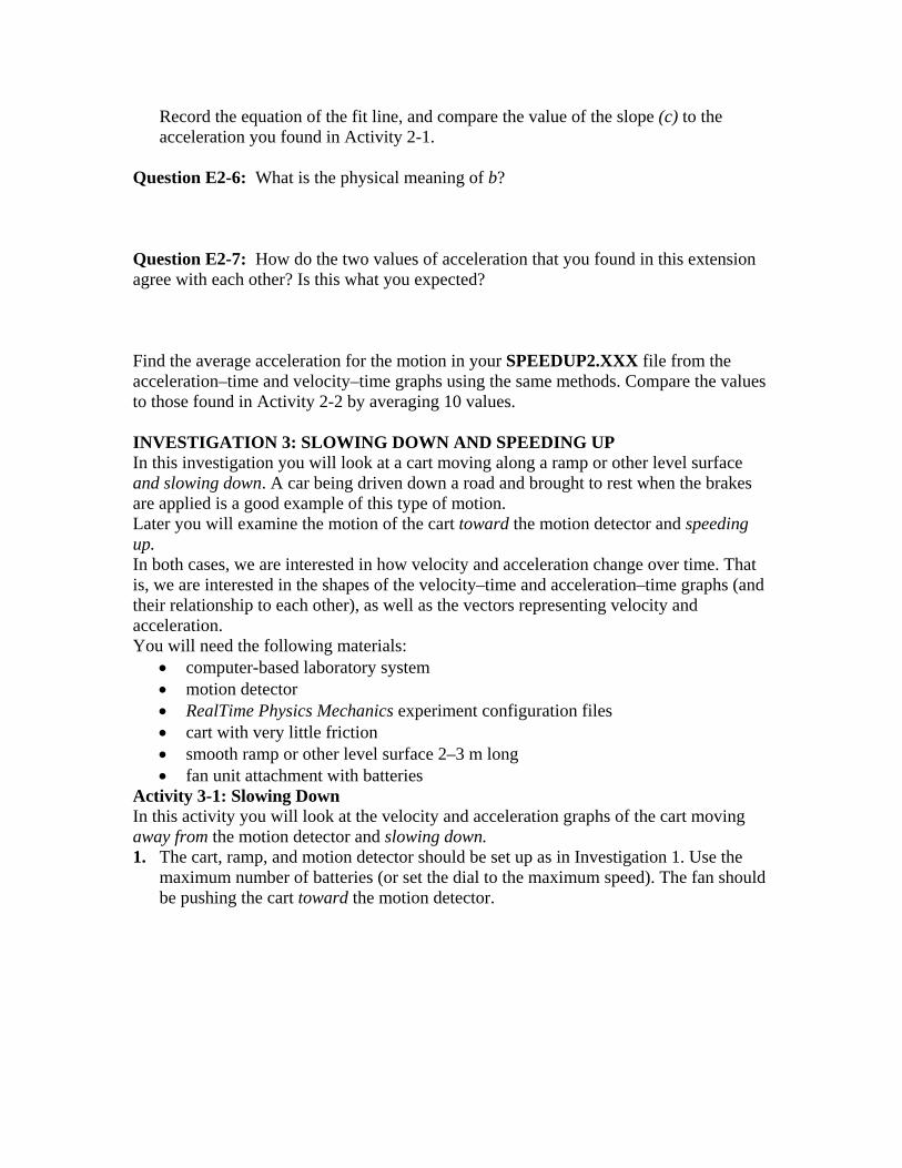
Activity 3-1: Slowing Down In this activity you will look at the velocity and acceleration graphs of the cart moving away from the motion detector and slowing down. 1. The cart, ramp, and motion detector should be set up as in Investigation 1. Use the

maximum number of batteries (or set the dial to the maximum speed). The fan should be pushing the cart toward the motion detector.

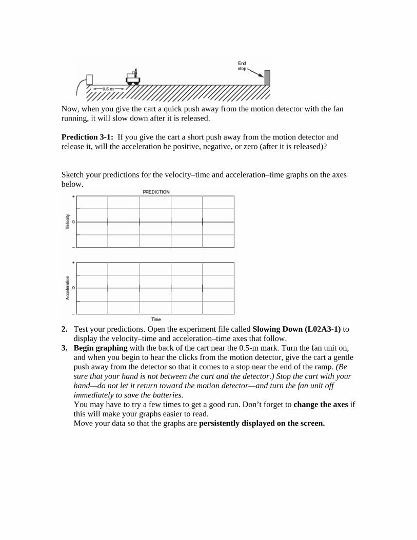
Now, when you give the cart a quick push away from the motion detector with the fan running, it will slow down after it is released. Prediction 3-1: If you give the cart a short push away from the motion detector and release it, will the acceleration be positive, negative, or zero (after it is released)? Sketch your predictions for the velocity–time and acceleration–time graphs on the axes below.

2. Test your predictions. Open the experiment file called Slowing Down (L02A3-1) to

display the velocity–time and acceleration–time axes that follow. 3. Begin graphing with the back of the cart near the 0.5-m mark. Turn the fan unit on,

and when you begin to hear the clicks from the motion detector, give the cart a gentle push away from the detector so that it comes to a stop near the end of the ramp. (Be sure that your hand is not between the cart and the detector.) Stop the cart with your hand—do not let it return toward the motion detector—and turn the fan unit off immediately to save the batteries. You may have to try a few times to get a good run. Don’t forget to change the axes if this will make your graphs easier to read. Move your data so that the graphs are persistently displayed on the screen.

4. Neatly sketch your results on the previous axes, or print the graphs and affix them

over the axes. Label your graphs with • A at the spot where you started pushing. • B at the spot where you stopped pushing. • C the region where only the force of the fan is acting on the cart • D at the spot where the cart came to rest (and you stopped it with your hand).

Also sketch on the same axes the velocity and acceleration graphs for Speeding Up 2 from Activity 1-2. Question 3-1: Did the shapes of your velocity and acceleration graphs agree with your predictions? How can you tell the sign of the acceleration from a velocity–time graph? Question 3-2: How can you tell the sign of the acceleration from an acceleration–time graph? Question 3-3: Is the sign of the acceleration (which indicates its direction) what you predicted? How does slowing down while moving away from the detector result in this sign of acceleration? (Hint: Remember that acceleration is the rate of change of velocity with respect to time. Look at how the velocity is changing.)

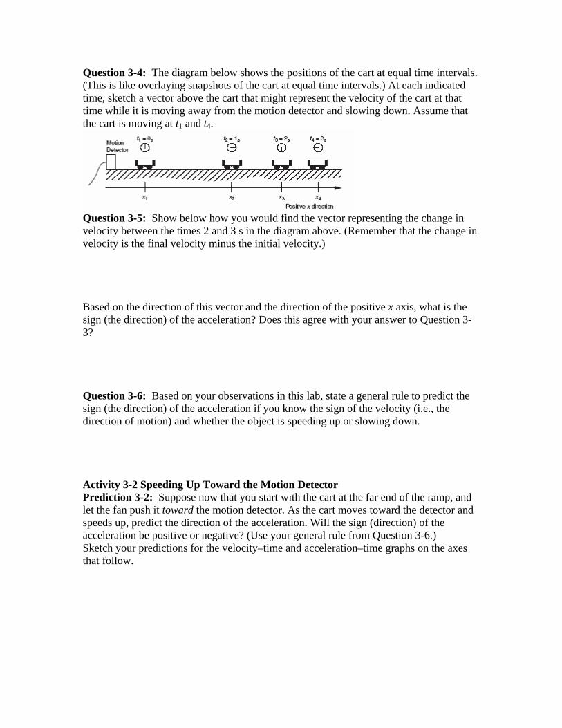
Question 3-4: The diagram below shows the positions of the cart at equal time intervals. (This is like overlaying snapshots of the cart at equal time intervals.) At each indicated time, sketch a vector above the cart that might represent the velocity of the cart at that time while it is moving away from the motion detector and slowing down. Assume that the cart is moving at t1 and t4.

Question 3-5: Show below how you would find the vector representing the change in velocity between the times 2 and 3 s in the diagram above. (Remember that the change in velocity is the final velocity minus the initial velocity.) Based on the direction of this vector and the direction of the positive x axis, what is the sign (the direction) of the acceleration? Does this agree with your answer to Question 3-3? Question 3-6: Based on your observations in this lab, state a general rule to predict the sign (the direction) of the acceleration if you know the sign of the velocity (i.e., the direction of motion) and whether the object is speeding up or slowing down. Activity 3-2 Speeding Up Toward the Motion Detector Prediction 3-2: Suppose now that you start with the cart at the far end of the ramp, and let the fan push it toward the motion detector. As the cart moves toward the detector and speeds up, predict the direction of the acceleration. Will the sign (direction) of the acceleration be positive or negative? (Use your general rule from Question 3-6.) Sketch your predictions for the velocity–time and acceleration–time graphs on the axes that follow.

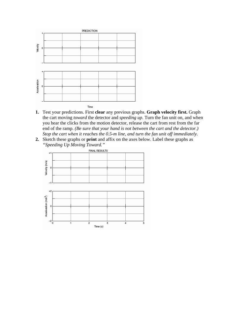
1. Test your predictions. First clear any previous graphs. Graph velocity first. Graph

the cart moving toward the detector and speeding up. Turn the fan unit on, and when you hear the clicks from the motion detector, release the cart from rest from the far end of the ramp. (Be sure that your hand is not between the cart and the detector.) Stop the cart when it reaches the 0.5-m line, and turn the fan unit off immediately.

2. Sketch these graphs or print and affix on the axes below. Label these graphs as “Speeding Up Moving Toward.”

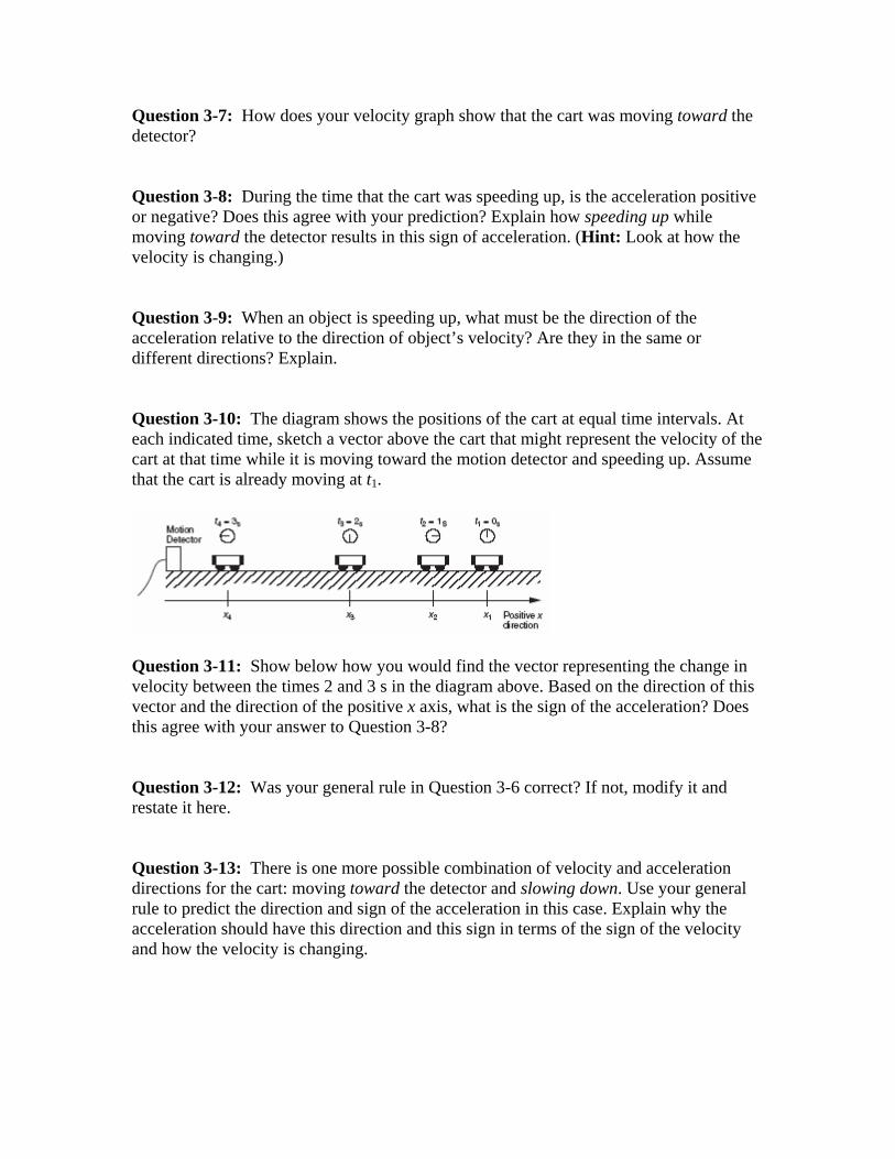
Question 3-7: How does your velocity graph show that the cart was moving toward the detector? Question 3-8: During the time that the cart was speeding up, is the acceleration positive or negative? Does this agree with your prediction? Explain how speeding up while moving toward the detector results in this sign of acceleration. (Hint: Look at how the velocity is changing.) Question 3-9: When an object is speeding up, what must be the direction of the acceleration relative to the direction of object’s velocity? Are they in the same or different directions? Explain. Question 3-10: The diagram shows the positions of the cart at equal time intervals. At each indicated time, sketch a vector above the cart that might represent the velocity of the cart at that time while it is moving toward the motion detector and speeding up. Assume that the cart is already moving at t1.

Question 3-11: Show below how you would find the vector representing the change in velocity between the times 2 and 3 s in the diagram above. Based on the direction of this vector and the direction of the positive x axis, what is the sign of the acceleration? Does this agree with your answer to Question 3-8? Question 3-12: Was your general rule in Question 3-6 correct? If not, modify it and restate it here. Question 3-13: There is one more possible combination of velocity and acceleration directions for the cart: moving toward the detector and slowing down. Use your general rule to predict the direction and sign of the acceleration in this case. Explain why the acceleration should have this direction and this sign in terms of the sign of the velocity and how the velocity is changing.

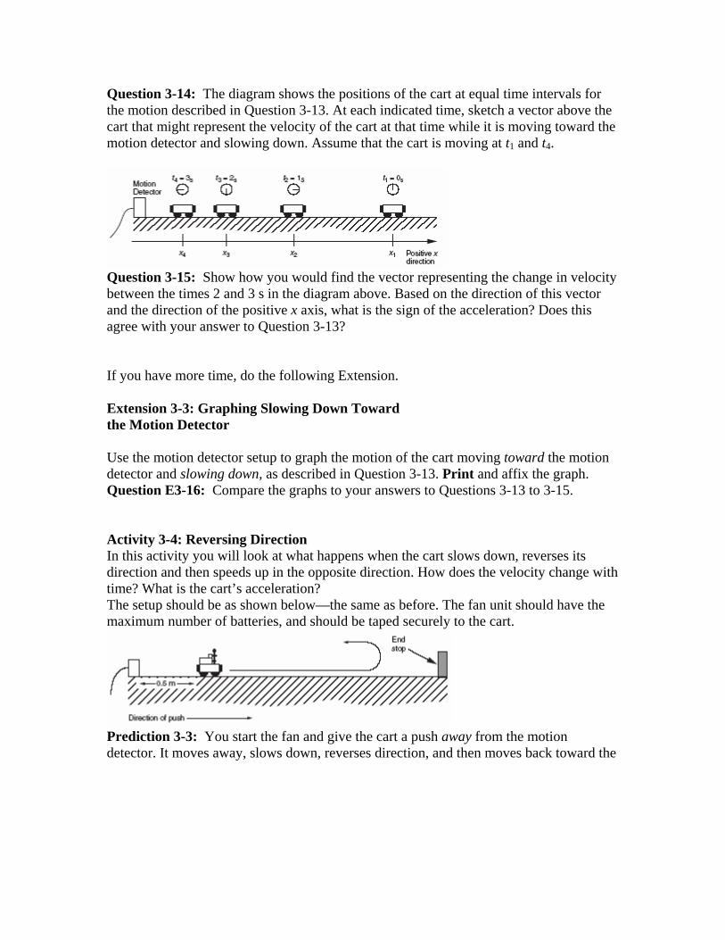
Question 3-14: The diagram shows the positions of the cart at equal time intervals for the motion described in Question 3-13. At each indicated time, sketch a vector above the cart that might represent the velocity of the cart at that time while it is moving toward the motion detector and slowing down. Assume that the cart is moving at t1 and t4.

Question 3-15: Show how you would find the vector representing the change in velocity between the times 2 and 3 s in the diagram above. Based on the direction of this vector and the direction of the positive x axis, what is the sign of the acceleration? Does this agree with your answer to Question 3-13? If you have more time, do the following Extension. Extension 3-3: Graphing Slowing Down Toward the Motion Detector Use the motion detector setup to graph the motion of the cart moving toward the motion detector and slowing down, as described in Question 3-13. Print and affix the graph. Question E3-16: Compare the graphs to your answers to Questions 3-13 to 3-15. Activity 3-4: Reversing Direction In this activity you will look at what happens when the cart slows down, reverses its direction and then speeds up in the opposite direction. How does the velocity change with time? What is the cart’s acceleration? The setup should be as shown below—the same as before. The fan unit should have the maximum number of batteries, and should be taped securely to the cart.

Prediction 3-3: You start the fan and give the cart a push away from the motion detector. It moves away, slows down, reverses direction, and then moves back toward the

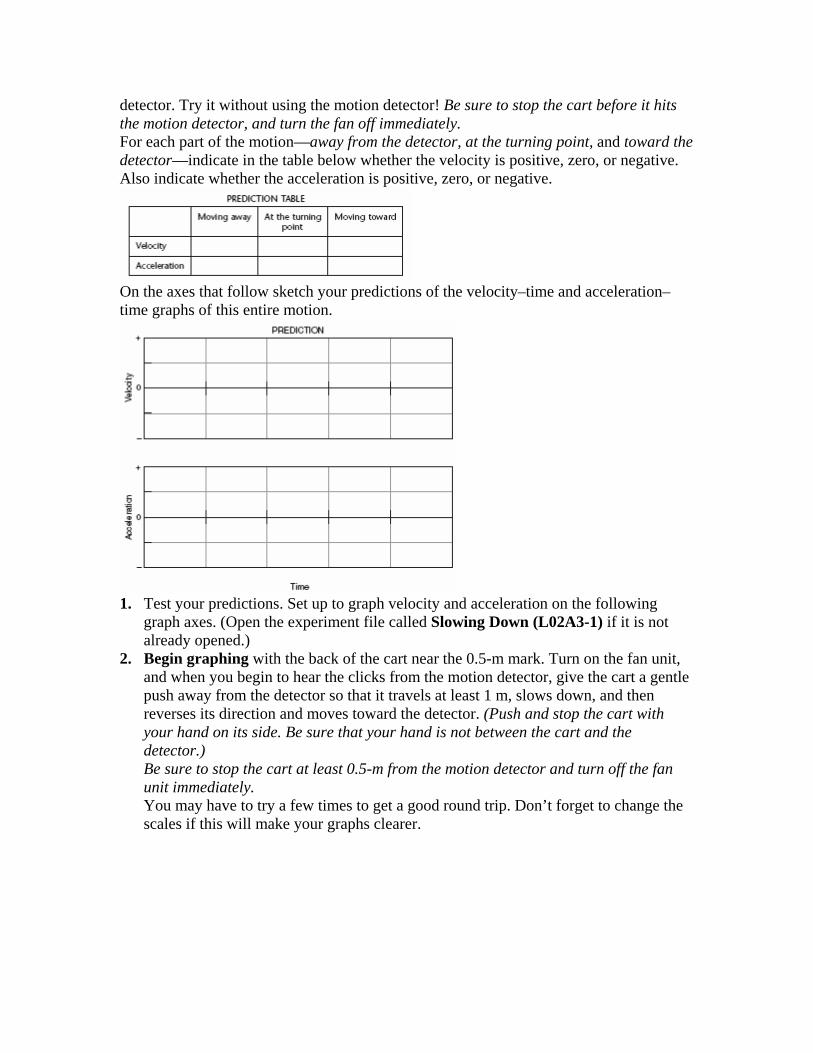
detector. Try it without using the motion detector! Be sure to stop the cart before it hits the motion detector, and turn the fan off immediately. For each part of the motion—away from the detector, at the turning point, and toward the detector—indicate in the table below whether the velocity is positive, zero, or negative. Also indicate whether the acceleration is positive, zero, or negative.

On the axes that follow sketch your predictions of the velocity–time and acceleration–time graphs of this entire motion.

1. Test your predictions. Set up to graph velocity and acceleration on the following

graph axes. (Open the experiment file called Slowing Down (L02A3-1) if it is not already opened.)

2. Begin graphing with the back of the cart near the 0.5-m mark. Turn on the fan unit, and when you begin to hear the clicks from the motion detector, give the cart a gentle push away from the detector so that it travels at least 1 m, slows down, and then reverses its direction and moves toward the detector. (Push and stop the cart with your hand on its side. Be sure that your hand is not between the cart and the detector.) Be sure to stop the cart at least 0.5-m from the motion detector and turn off the fan unit immediately. You may have to try a few times to get a good round trip. Don’t forget to change the scales if this will make your graphs clearer.

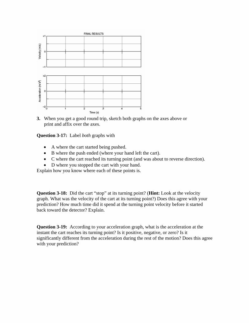
3. When you get a good round trip, sketch both graphs on the axes above or

print and affix over the axes. Question 3-17: Label both graphs with

• A where the cart started being pushed. • B where the push ended (where your hand left the cart). • C where the cart reached its turning point (and was about to reverse direction). • D where you stopped the cart with your hand.

Explain how you know where each of these points is. Question 3-18: Did the cart “stop” at its turning point? (Hint: Look at the velocity graph. What was the velocity of the cart at its turning point?) Does this agree with your prediction? How much time did it spend at the turning point velocity before it started back toward the detector? Explain. Question 3-19: According to your acceleration graph, what is the acceleration at the instant the cart reaches its turning point? Is it positive, negative, or zero? Is it significantly different from the acceleration during the rest of the motion? Does this agree with your prediction?

Question 3-20: Explain the observed sign of the acceleration at the turning point. (Hint: Remember that acceleration is the rate of change of velocity. When the cart is at its turning point, what will its velocity be in the next instant? Will it be positive or negative?) Question 3-21: On the way back toward the detector, is there any difference between these velocity and acceleration graphs and the ones that were the result of the cart starting from rest (Activity 3-2)? Explain. If you have more time, do the following Extension. Extension 3-5: Sign of Push and Stop

Find on your acceleration graphs for Activity 3-4 the time intervals when you pushed the cart to start it moving and when you stopped it. Question E3-22: What is the sign of the acceleration for each of these intervals? Explain why the acceleration has this sign in each case. Challenge: You throw a ball up into the air. It moves upward, reaches its highest point, and then moves back down toward your hand. Assuming that upward is the positive direction, indicate in the table that follows whether the velocity is positive, zero, or negative during each of the three parts of the motion. Also indicate if the acceleration is positive, zero, or negative. (Hint: Remember that to find the acceleration, you must look at the change in velocity.)

Question 3-23: In what ways is the motion of the ball similar to the motion of the cart that you just observed? What causes the ball to accelerate?

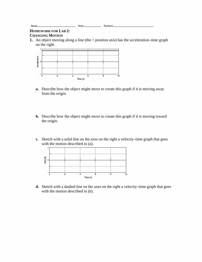
HOMEWORK FOR LAB 2: CHANGING MOTION 1. An object moving along a line (the + position axis) has the acceleration–time graph

on the right.

a. Describe how the object might move to create this graph if it is moving away from the origin.

b. Describe how the object might move to create this graph if it is moving toward the origin.

c. Sketch with a solid line on the axes on the right a velocity–time graph that goes with the motion described in (a).

d. Sketch with a dashed line on the axes on the right a velocity–time graph that goes with the motion described in (b).

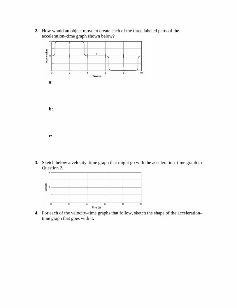
2. How would an object move to create each of the three labeled parts of the acceleration–time graph shown below?

a: b: c: 3. Sketch below a velocity–time graph that might go with the acceleration–time graph in

Question 2.

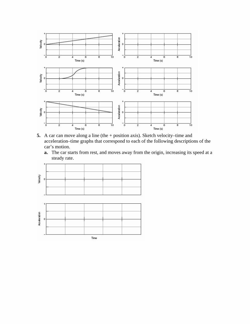
4. For each of the velocity–time graphs that follow, sketch the shape of the acceleration–

time graph that goes with it.

5. A car can move along a line (the + position axis). Sketch velocity–time and

acceleration–time graphs that correspond to each of the following descriptions of the car’s motion. a. The car starts from rest, and moves away from the origin, increasing its speed at a

steady rate.

b. The car is moving away from the origin at a constant velocity.

c. The car starts from rest, and moves away from the origin, increasing its speed at a steady rate twice as large as in (a) above.

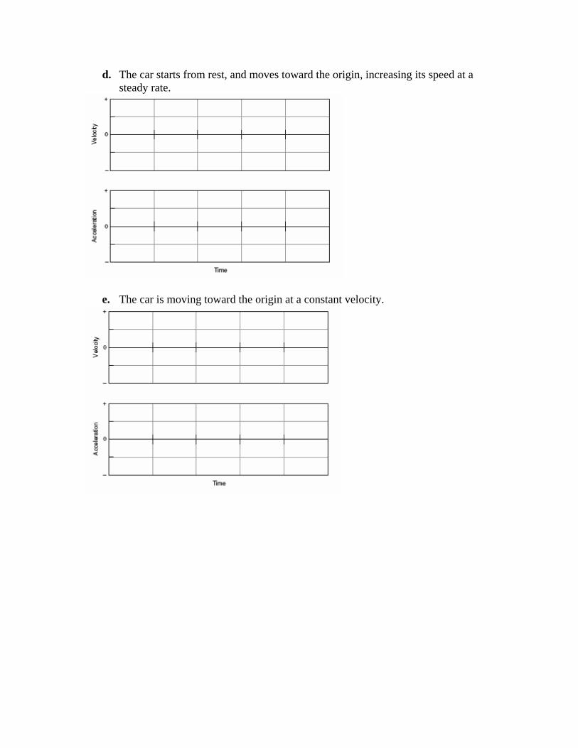
d. The car starts from rest, and moves toward the origin, increasing its speed at a steady rate.

e. The car is moving toward the origin at a constant velocity.

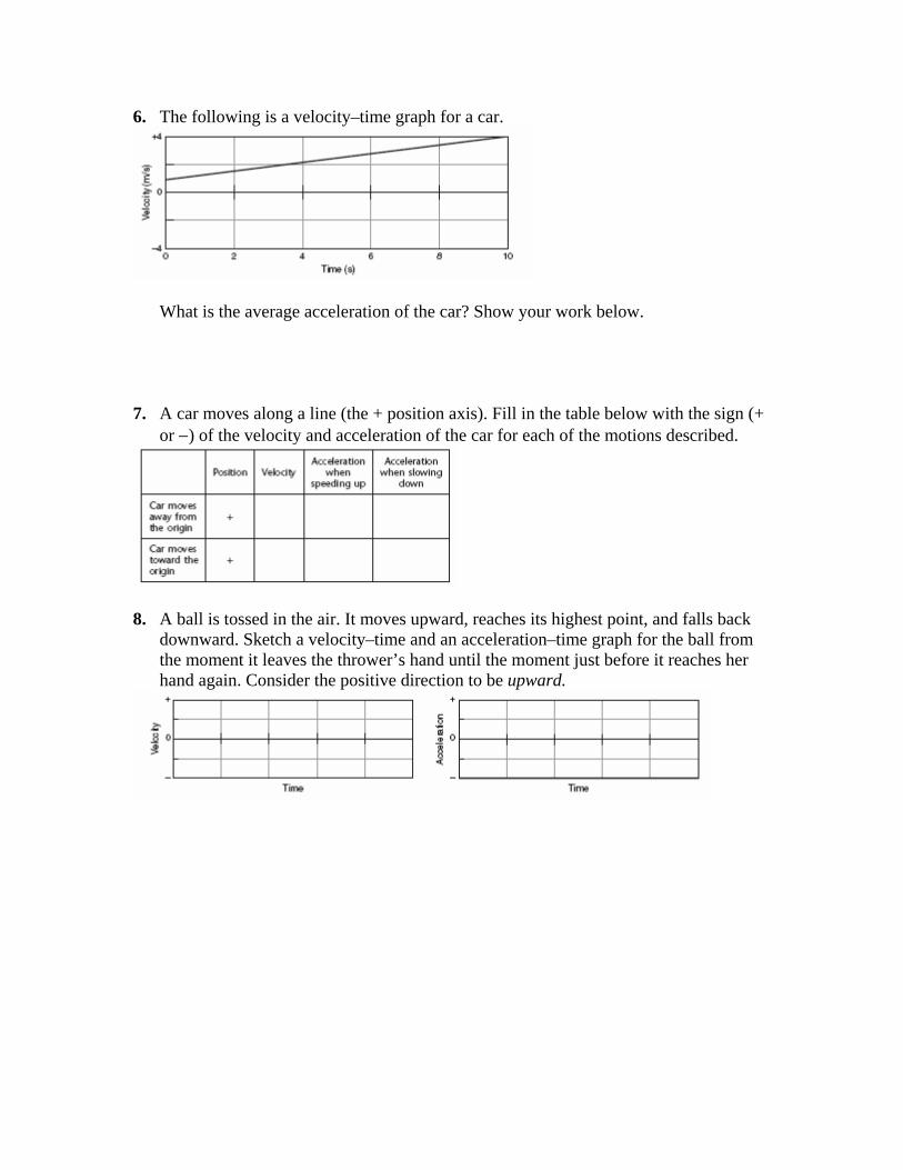
6. The following is a velocity–time graph for a car.

What is the average acceleration of the car? Show your work below. 7. A car moves along a line (the + position axis). Fill in the table below with the sign (+

or −) of the velocity and acceleration of the car for each of the motions described.

8. A ball is tossed in the air. It moves upward, reaches its highest point, and falls back

downward. Sketch a velocity–time and an acceleration–time graph for the ball from the moment it leaves the thrower’s hand until the moment just before it reaches her hand again. Consider the positive direction to be upward.

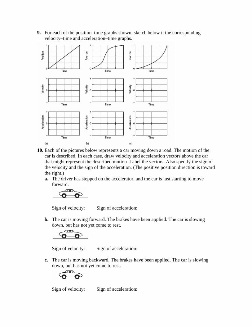
9. For each of the position–time graphs shown, sketch below it the corresponding velocity–time and acceleration–time graphs.

10. Each of the pictures below represents a car moving down a road. The motion of the

car is described. In each case, draw velocity and acceleration vectors above the car that might represent the described motion. Label the vectors. Also specify the sign of the velocity and the sign of the acceleration. (The positive position direction is toward the right.) a. The driver has stepped on the accelerator, and the car is just starting to move

forward.

Sign of velocity: Sign of acceleration:

b. The car is moving forward. The brakes have been applied. The car is slowing down, but has not yet come to rest.

Sign of velocity: Sign of acceleration:

c. The car is moving backward. The brakes have been applied. The car is slowing down, but has not yet come to rest.

Sign of velocity: Sign of acceleration:

11. a. Describe how you would move to produce the velocity–time graph below.

b. Sketch a position–time graph for this motion on the axes below.

c. Sketch an acceleration–time graph for this motion on the axes below.

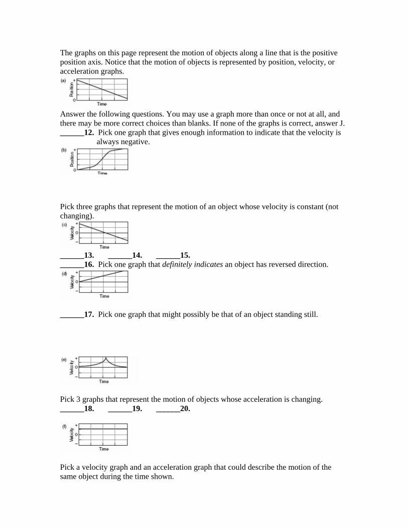
The graphs on this page represent the motion of objects along a line that is the positive position axis. Notice that the motion of objects is represented by position, velocity, or acceleration graphs.

Answer the following questions. You may use a graph more than once or not at all, and there may be more correct choices than blanks. If none of the graphs is correct, answer J. ______12. Pick one graph that gives enough information to indicate that the velocity is

always negative.

Pick three graphs that represent the motion of an object whose velocity is constant (not changing).

______13. ______14. ______15. ______16. Pick one graph that definitely indicates an object has reversed direction.

______17. Pick one graph that might possibly be that of an object standing still.

Pick 3 graphs that represent the motion of objects whose acceleration is changing. ______18. ______19. ______20.

Pick a velocity graph and an acceleration graph that could describe the motion of the same object during the time shown.

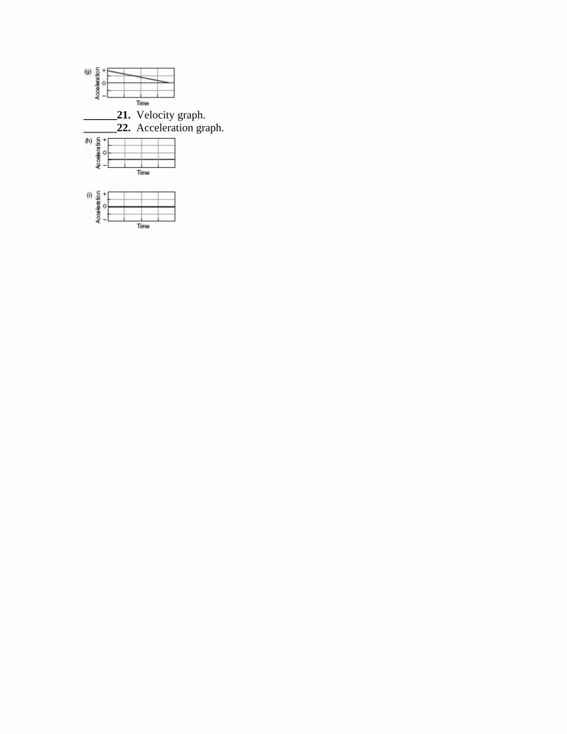
______21. Velocity graph. ______22. Acceleration graph.