Pre-requisite Material for Course Heuristics and ... · Pre-requisite Material for Course ... Basics of Heuristic Search for Optimization 7 2.1. Optimization Problems 7 2.2. Linear

NATCOR at UoN - Heuristics and Approximation Algorithms 9-13 April 2018

ASAP Research Group, School of Computer Science, The University of Nottingham Page 1

Pre-requisite Material for Course ‘Heuristics and Approximation Algorithms’ This document contains an overview of the basic concepts that are needed in preparation to participate in the course. In addition, it will be useful that students have some experience with Java programming and probability theory but this is desirable, not a mandatory pre-requisite. At the start of the course, students will be asked to indicate their level of expertise in these topics in order to inform the delivery of the course. Additional Material for the Course https://drive.google.com/drive/folders/1OJ6V1ruozde2UIWO89PyD6q-ycP9ZKOx

Contents Page 1. Basics of Complexity Theory 2

1.1. Computability 2

1.2. Computational Problems 2

1.3. Computational Algorithms 3

1.4. Intractable and Undecidable Problems 4

1.5. Time Complexity 4

1.6. Tackling NP-Complete Problems 6

2. Basics of Heuristic Search for Optimization 7

2.1. Optimization Problems 7

2.2. Linear Programming (LP) 8

2.3. Integer Programming (IP) 8

2.4. Discrete/Continuous/Combinatorial Optimization 9

2.5. Approximation Algorithms 10

2.6. Greedy Algorithms and Neighbourhood Search 11

2.7. Basics of Meta-heuristics 14

2.8. Basics of Evolutionary Algorithms 15

https://drive.google.com/drive/folders/1OJ6V1ruozde2UIWO89PyD6q-ycP9ZKOx



1. Basics of Complexity Theory

1.1 Computability

Computability focuses on answering questions such as:

What class of problems can be solved using a computational algorithm?

Is there an efficient computational algorithm to solve a given problem?

There have been many attempts by computer scientists to define precisely what is an effective

procedure or computable function.

Intuitively, a computable function can be implemented on a computer, whether in a reasonable

computational time or not.

An ideal formulation of an effective procedure or computable function involves:

1. A language in which a set of rules can be expressed.

2. A rigorous description of a single machine which can interpret the rules in the given language

and carry out the steps of a specified process.

1.2 Computational Problems

The classical Travelling Salesman Problem (TSP): Given a set of c cities 1,2,…,c and the distance d(i,j)

(a non-negative integer ) between two cities i and j, find the shortest tour of the cities.

The TSP is one of the most intensively studied problems in mathematics and computer science.

A computational problem (e.g. the classical TSP) is generally described by:

• Its parameters (e.g. set of cities, distance between cities)

• Statement of the required properties in the solution (e.g. ordering of the cities such that the

travelling distance is minimised)

An instance of a computational problem gives specific values to the problem parameters and a

solution to that instance has a specific value.

The size of a problem instance is defined in terms of the amount of input data required to describe

its parameters.

In practice, the instance size is conveniently expressed in terms of a single variable.

For example, the size of an instance of the travelling salesman problem (TSP) can be expressed by:

• A finite input string describing exactly all parameter values (cities and distances)

• A number intending to reflect the size of the input string (number of cities)



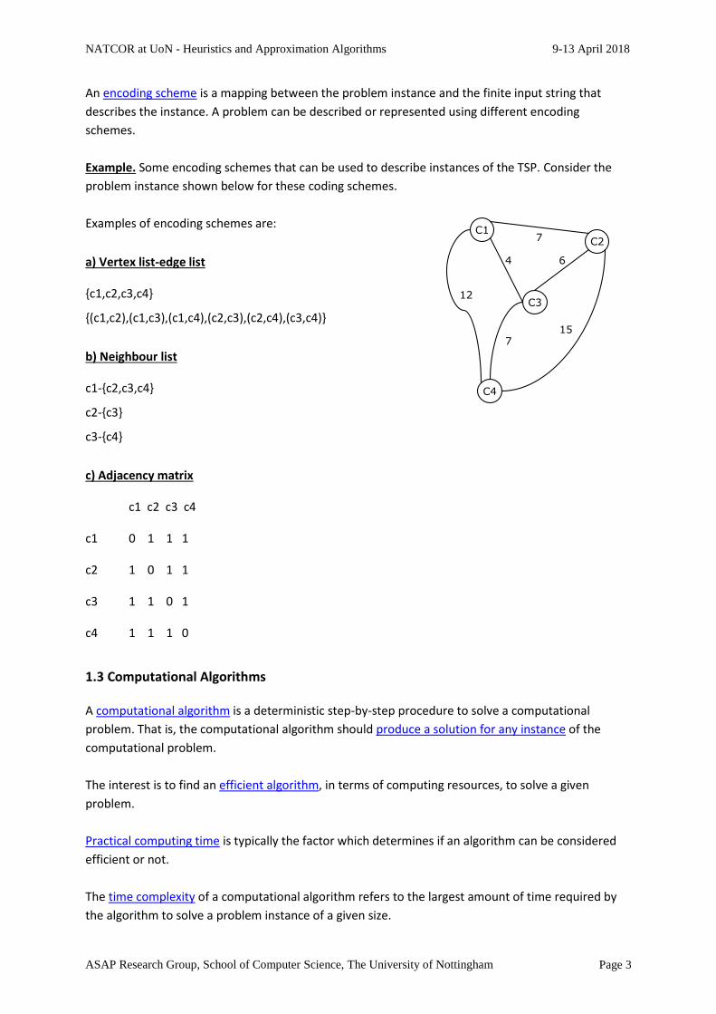
An encoding scheme is a mapping between the problem instance and the finite input string that

describes the instance. A problem can be described or represented using different encoding

schemes.

Example. Some encoding schemes that can be used to describe instances of the TSP. Consider the

problem instance shown below for these coding schemes.

Examples of encoding schemes are:

a) Vertex list-edge list

{c1,c2,c3,c4}

{(c1,c2),(c1,c3),(c1,c4),(c2,c3),(c2,c4),(c3,c4)}

b) Neighbour list

c1-{c2,c3,c4}

c2-{c3}

c3-{c4}

c) Adjacency matrix

c1 c2 c3 c4

c1 0 1 1 1

c2 1 0 1 1

c3 1 1 0 1

c4 1 1 1 0

1.3 Computational Algorithms

A computational algorithm is a deterministic step-by-step procedure to solve a computational

problem. That is, the computational algorithm should produce a solution for any instance of the

computational problem.

The interest is to find an efficient algorithm, in terms of computing resources, to solve a given

problem.

Practical computing time is typically the factor which determines if an algorithm can be considered

efficient or not.

The time complexity of a computational algorithm refers to the largest amount of time required by

the algorithm to solve a problem instance of a given size.

4 6

7

7

15

12

C4

C1 C2

C3



For a given problem, how to assess if a computational algorithm is efficient?

Computational perspective: polynomial time vs. exponential time complexity.

The complexity of a function f(n) is O(g(n)) if |f(n)| ≤ c|g(n)| for all n>0 and some constant c.

An algorithm has polynomial time complexity if its complexity function is given by O(g(n)) where g(n)

is a polynomial function for the input length n.

1.4 Intractable and Undecidable Problems

A computational problem is considered intractable if no computationally efficient algorithm can be

given to solve it, or in other words, if no polynomial time algorithm can be found to solve it.

Although polynomial time algorithms are preferred, some exponential time algorithms are

considered good to solve some problems. This is because the algorithm may have exponential

complexity in the worst case but it performs satisfactorily on the average.

The tractability of a given problem is independent of the encoding scheme and the computer model.

The tractability of a problem can refer to:

• An exponential amount of computational time is needed to find a solution. For example

solving the TSP with algorithm A3.

• A solution is too long that cannot be described with a polynomial expression on the length of

the input. For example, in a TSP instance, asking for all tours that have length L or less.

A computational problem is considered undecidable if there is no algorithm at all can be given to

solve it. Therefore, an undecidable problem is also intractable.

Many intractable problems are decidable and can be solved in polynomial time with a non-

deterministic computing model.

The NP-complete class of problems include decision problems (the answer is either YES or NO) that

can be solved by a non-deterministic computing model in polynomial time.

The conjecture is that NP-complete problems are intractable but this is a very much open question.

But at least, if the problem is NP-complete there is no known polynomial time algorithm to solve it.

1.5 Time Complexity

We attempt to separate the practically solvable problems from those that cannot be solved in a

reasonable time.



When constructing a computer algorithm it is important to assess how expensive the algorithm is in

terms of storage and time.

Algorithm complexity analysis tells how much time does an algorithm takes to solve a problem.

The size of a problem instance is typically measured by the size of the input that describes the given

instance.

Algorithm complexity analysis is based on counting primitive operations such as arithmetic, logical,

reads, writes, data retrieval, data storage, etc.

timeA(n) expresses the time complexity of algorithm A and is defined as the greatest number of

primitive operations that could be performed by the algorithm given a problem

instance of size n.

We are usually more interested in the rate of growth of timeA than in the actual number of

operations in the algorithm.

Thus, to determine whether it is practical or feasible to implement A we require a not too large

upper bound for timeA(n).

Time complexity of algorithms is expressed using the O-notation.

The complexity of a function f(n) is O(g(n)) if |f(n)| ≤ c|g(n)| for all n>0 and some constant c.

Let f and g be functions on n, then:

f(n) = O(g(n)) means that “f is of the order of g”, that is, “f grows at the same rate of g or slower”.

f(n) = (g(n)) means that “f grows faster than g”

f(n) = (g(n)) means that “f and g grow at the same rate”.

An algorithm is said to perform in polynomial time if and only if its time complexity function is given

by O(nk) for some k 0.

That is, an algorithm A is polynomial time if timeA(n) f(n) and f is a polynomial, i.e. f has the form:

a1nk + a2nk-1 +…+ am

Then, the class P is defined as the class of problems which can be solved by polynomial time

deterministic algorithms. The notion is that problems in P can be solved ‘quickly’.

Then, the class NP is defined as the class of problems which can be solved by polynomial time non-

deterministic algorithms. The notion is that problems in NP can be verified ‘quickly’.



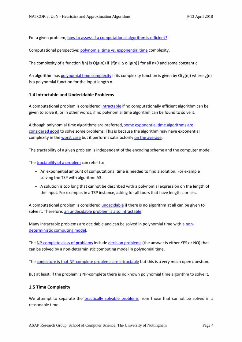
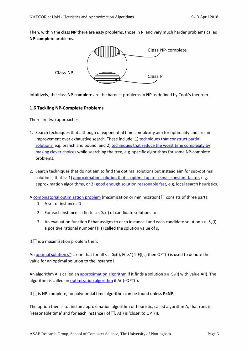
Then, within the class NP there are easy problems, those in P, and very much harder problems called

NP-complete problems.

Intuitively, the class NP-complete are the hardest problems in NP as defined by Cook’s theorem.

1.6 Tackling NP-Complete Problems

There are two approaches:

1. Search techniques that although of exponential time complexity aim for optimality and are an

improvement over exhaustive search. These include: 1) techniques that construct partial

solutions, e.g. branch and bound, and 2) techniques that reduce the worst time complexity by

making clever choices while searching the tree, e.g. specific algorithms for some NP-complete

problems.

2. Search techniques that do not aim to find the optimal solutions but instead aim for sub-optimal

solutions, that is: 1) approximation solution that is optimal up to a small constant factor, e.g.

approximation algorithms, or 2) good enough solution reasonable fast, e.g. local search heuristics.

A combinatorial optimization problem (maximization or minimization) consists of three parts:

1. A set of instances D

2. For each instance I a finite set SD(I) of candidate solutions to I

3. An evaluation function F that assigns to each instance I and each candidate solution s SD(I)

a positive rational number F(I,s) called the solution value of s.

If is a maximisation problem then:

An optimal solution s* is one that for all s SD(I), F(I,s*) ≥ F(I,s) then OPT(I) is used to denote the

value for an optimal solution to the instance I.

An algorithm A is called an approximation algorithm if it finds a solution s SD(I) with value A(I). The

algorithm is called an optimization algorithm if A(I)=OPT(I).

If is NP-complete, no polynomial time algorithm can be found unless P=NP.

The option then is to find an approximation algorithm or heuristic, called algorithm A, that runs in

‘reasonable time’ and for each instance I of , A(I) is ‘close’ to OPT(I).

Class NP-complete

Class NP Class P



2. Basics of Heuristic Search for Optimization

2.1 Optimization Problems

Basic ingredients of optimization problems:

A set of decision variables which affect the value of the objective function. In the travelling

salesman problem, the variables might be of the type Xij {0,1} where the value of the

variable indicates whether city j is visited after city i or not; in fitting-the-data problem, the

variables are the parameters that define the model.

An objective function which we want to minimize or maximize. It relates the decision variables

to the goal and measures goal attainment. For instance, in the travelling salesman problem,

we want to minimise the total distance travelled for visiting all cities in a tour; in fitting

experimental data to a user-defined model, we might minimize the total deviation of observed

data from predictions based on the model.

A set of constraints that allow the variables to take on certain values but exclude others. For

some variations of the travelling salesman problem, it may not be allowed to visit some cities

in a certain sequence, so restricting the values that certain decision variables can take in a

solution to the problem instance.

The optimization problem is defined as follows:

Find values for all the decision variables that minimize or maximize the objective function while

satisfying the given constraints.

Formal representation of optimization problems are described by mathematical programming.

Mathematical programming is used to describe problems of choosing the best element from some

set of available alternatives or in OR terms to describe problems how to allocate limited resources.

Mathematical formulation:

minimize f(x)

subject to

gi(x) ≥bi, i=1,…,m

hj(x) =cj, j=1,…,n

where x is a vector of decision variables, f(),gi(), hi() are general functions.

Similar formulation of the problem holds when the objective function has to be maximized.

Placing restrictions on the type of functions under consideration and on the values that the decision

variables can take lead to specific classes of optimization problems.

A solution which satisfies all constraints is called a feasible solution.



2.2 Linear Programming (LP)

• In an LP formulation, f(),gi(), hi() are linear functions of decision variables

• LP is one of the most important tools in OR

• The typical LP problem involves:

− limited resources − competing activities − measure of solution quality − constraints on the use of resources − the optimal solution

• LP is a mathematical model with:

− decision variables and parameters − linear algebraic expressions (objective function and constraints) − planning activities

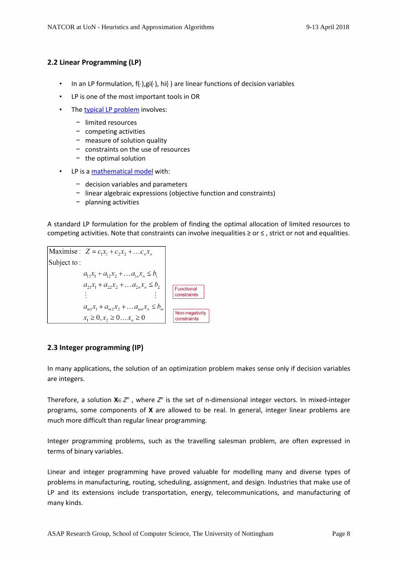
A standard LP formulation for the problem of finding the optimal allocation of limited resources to competing activities. Note that constraints can involve inequalities ≥ or ≤ , strict or not and equalities.

2.3 Integer programming (IP)

In many applications, the solution of an optimization problem makes sense only if decision variables

are integers.

Therefore, a solution XZn , where Zn is the set of n-dimensional integer vectors. In mixed-integer

programs, some components of X are allowed to be real. In general, integer linear problems are

much more difficult than regular linear programming.

Integer programming problems, such as the travelling salesman problem, are often expressed in

terms of binary variables.

Linear and integer programming have proved valuable for modelling many and diverse types of

problems in manufacturing, routing, scheduling, assignment, and design. Industries that make use of

LP and its extensions include transportation, energy, telecommunications, and manufacturing of

many kinds.

http://wiki.mcs.anl.gov/NEOS/index.php/Mixed_Integer_Programming

http://wiki.mcs.anl.gov/NEOS/index.php/Mixed_Integer_Programming



2.4 Discrete/Continuous/Combinatorial Optimization

In discrete optimization, the variables used in the mathematical programming formulation are restricted to assume only discrete values, such as the integers. In continuous optimization, the variables used in the objective function can assume real values, e.g., values from intervals of the real line. In combinatorial optimization, decision variables are discrete, which means that the solution is a set, or sequence of integers or other discrete objects. The number of possible solutions is combinatorial number (extra large number, such as 1050). Combinatorial optimization problems include problems on graphs, matroids and other discrete structures. An example of combinatorial optimization is the set covering problem. Given a finite set of N items

and a set of available features U, the problem is to select the smallest subset of items that together

include the subset F U of desirable features. Assume that cij=1 if item i includes feature j, otherwise

cij=0.

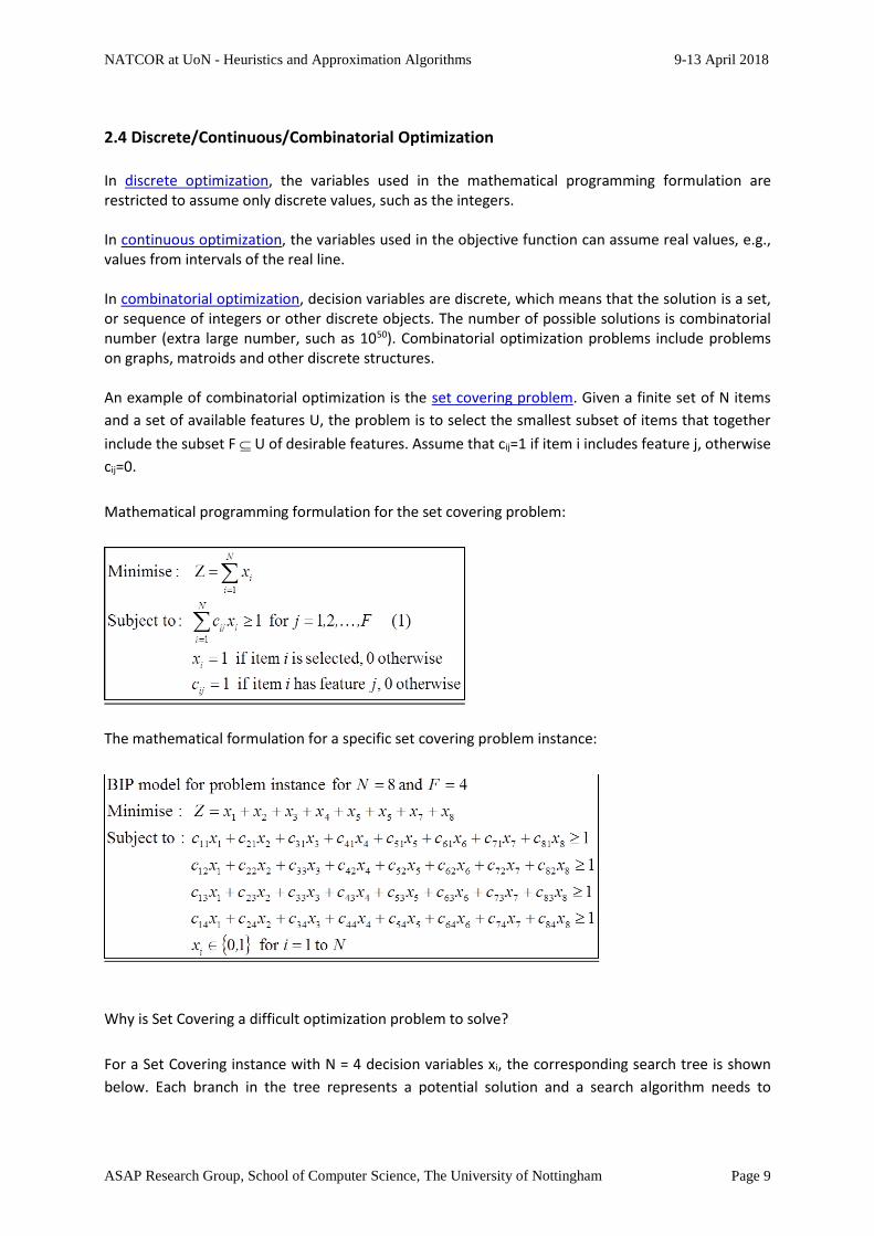
Mathematical programming formulation for the set covering problem:

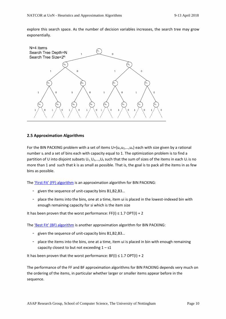
The mathematical formulation for a specific set covering problem instance:

Why is Set Covering a difficult optimization problem to solve?

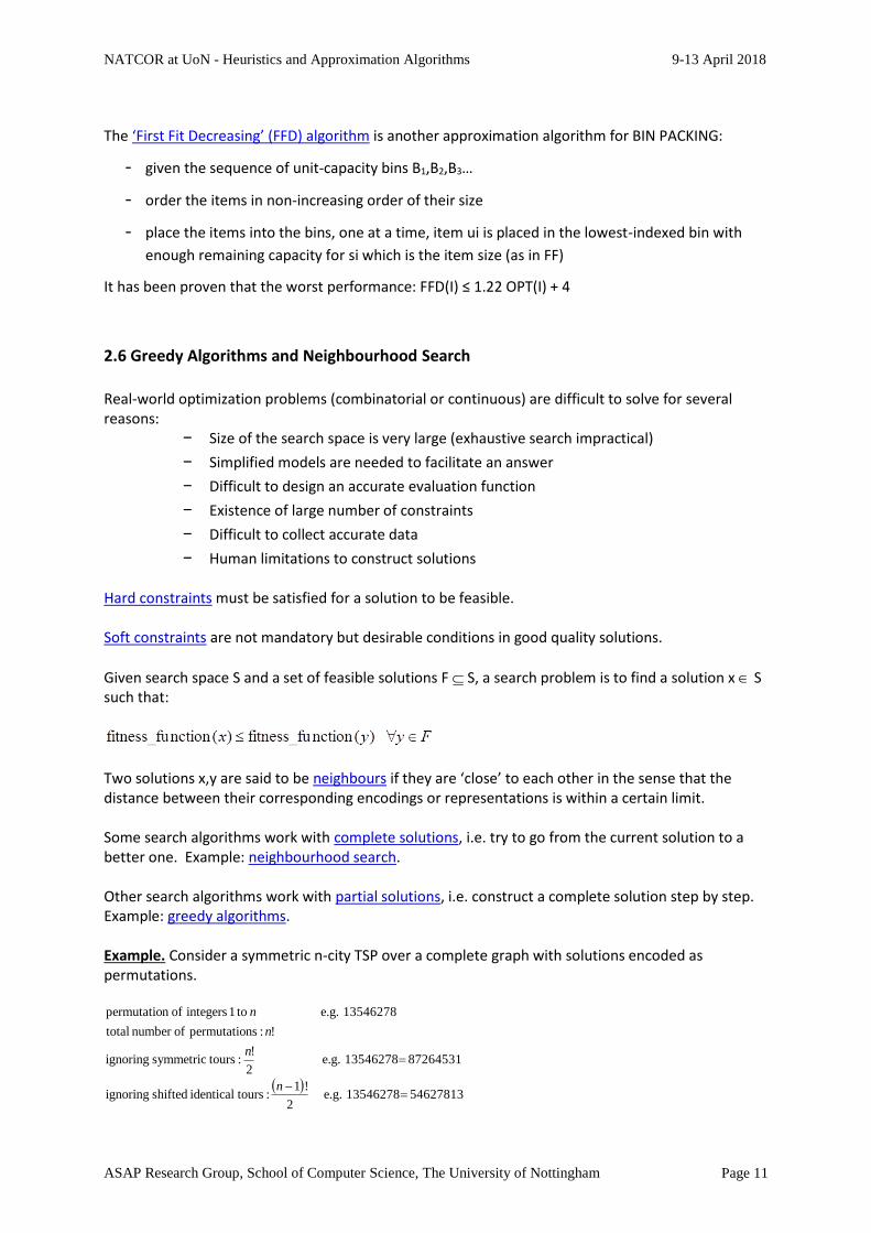
For a Set Covering instance with N = 4 decision variables xi, the corresponding search tree is shown

below. Each branch in the tree represents a potential solution and a search algorithm needs to

http://en.wikipedia.org/wiki/Variable_%28mathematics%29

http://en.wikipedia.org/wiki/Optimization_%28mathematics%29

http://en.wikipedia.org/wiki/Real_number



explore this search space. As the number of decision variables increases, the search tree may grow

exponentially.

2.5 Approximation Algorithms

For the BIN PACKING problem with a set of items U={ui,u2,…,un} each with size given by a rational

number si and a set of bins each with capacity equal to 1. The optimization problem is to find a

partition of U into disjoint subsets U1, U2,…,Uk such that the sum of sizes of the items in each Ui is no

more than 1 and such that k is as small as possible. That is, the goal is to pack all the items in as few

bins as possible.

The ‘First Fit’ (FF) algorithm is an approximation algorithm for BIN PACKING:

- given the sequence of unit-capacity bins B1,B2,B3…

- place the items into the bins, one at a time, item ui is placed in the lowest-indexed bin with

enough remaining capacity for si which is the item size

It has been proven that the worst performance: FF(I) ≤ 1.7 OPT(I) + 2

The ‘Best Fit’ (BF) algorithm is another approximation algorithm for BIN PACKING:


- place the items into the bins, one at a time, item ui is placed in bin with enough remaining

capacity closest to but not exceeding 1 – s1

It has been proven that the worst performance: BF(I) ≤ 1.7 OPT(I) + 2

The performance of the FF and BF approximation algorithms for BIN PACKING depends very much on

the ordering of the items, in particular whether larger or smaller items appear before in the

sequence.



The ‘First Fit Decreasing’ (FFD) algorithm is another approximation algorithm for BIN PACKING:


- order the items in non-increasing order of their size

- place the items into the bins, one at a time, item ui is placed in the lowest-indexed bin with

enough remaining capacity for si which is the item size (as in FF)

It has been proven that the worst performance: FFD(I) ≤ 1.22 OPT(I) + 4

2.6 Greedy Algorithms and Neighbourhood Search

Real-world optimization problems (combinatorial or continuous) are difficult to solve for several reasons:

− Size of the search space is very large (exhaustive search impractical)

− Simplified models are needed to facilitate an answer

− Difficult to design an accurate evaluation function

− Existence of large number of constraints

− Difficult to collect accurate data

− Human limitations to construct solutions Hard constraints must be satisfied for a solution to be feasible. Soft constraints are not mandatory but desirable conditions in good quality solutions.

Given search space S and a set of feasible solutions F S, a search problem is to find a solution x S such that:

Two solutions x,y are said to be neighbours if they are ‘close’ to each other in the sense that the distance between their corresponding encodings or representations is within a certain limit. Some search algorithms work with complete solutions, i.e. try to go from the current solution to a better one. Example: neighbourhood search. Other search algorithms work with partial solutions, i.e. construct a complete solution step by step. Example: greedy algorithms. Example. Consider a symmetric n-city TSP over a complete graph with solutions encoded as permutations.

54627813 13546278 e.g.

2

! 1 : toursidentical shifted ignoring

87264531 13546278 e.g. 2

!: tourssymmetric ignoring

! :nspermutatio ofnumber total

13546278 e.g. to1 integers ofn permutatio

n

n

n

n



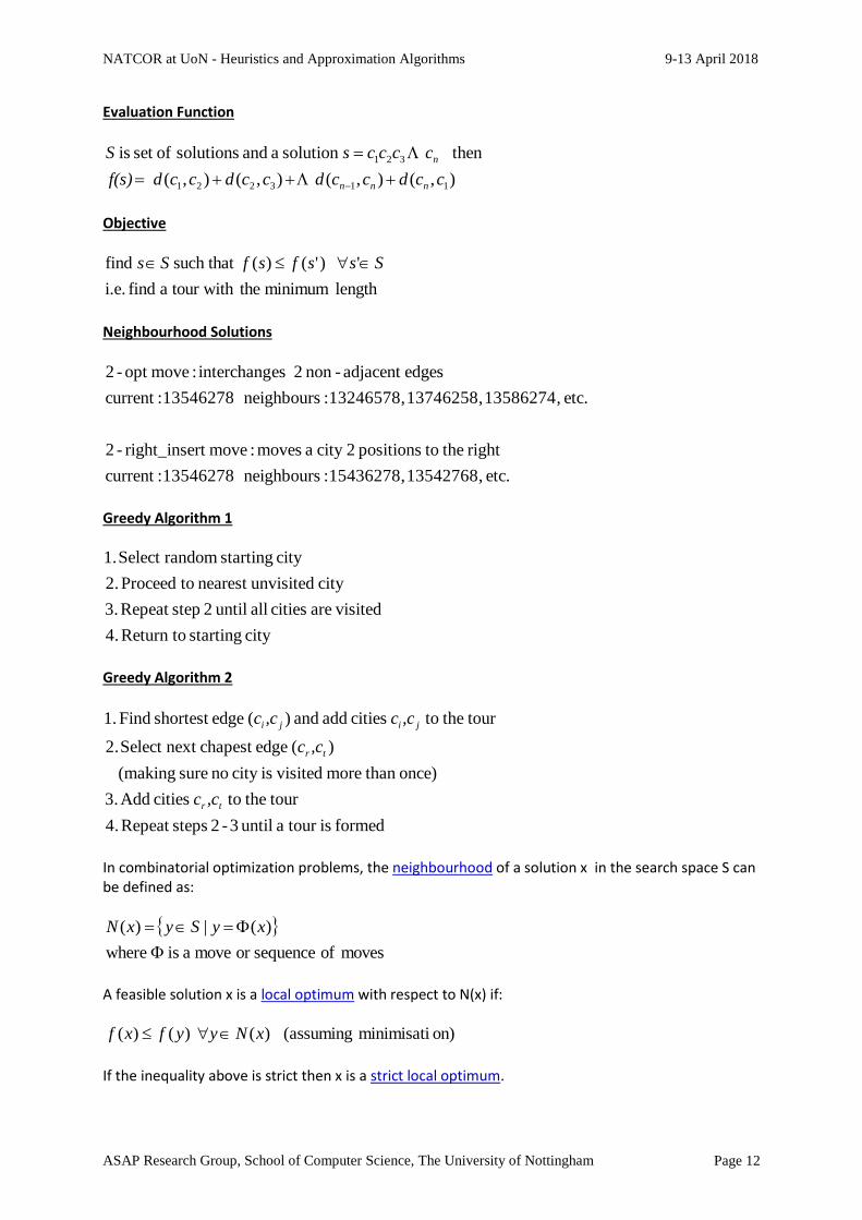
Evaluation Function

),(),(),(),(

thensolution a and solutions ofset is

113221

321

ccdccdccdcc df(s)

ccccsS

nnn

n

Objective

length minimum the tour witha find i.e.

' )'()(such that find SssfsfSs

Neighbourhood Solutions

etc. , 13542768 , 15436278 :neighbours 13546278 :current

right the topositions 2city a moves :movert right_inse-2

etc. , 13586274 , 13746258 , 13246578 :neighbours 13546278 :current

edgesadjacent -non 2 esinterchang :moveopt -2

Greedy Algorithm 1

city starting Return to 4.

visitedare cities all until 2 stepRepeat 3.

city unvisitednearest toProceed 2.

city starting randomSelect .1

Greedy Algorithm 2

formed is tour a until 3-2 stepsRepeat 4.

tour the to cities Add 3.

once) than more visitediscity no sure (making

)( edgechapest next Select 2.

tour the to cities add and )( edgeshortest Find .1

tr

tr

jiji

,cc

,cc

,cc,cc

In combinatorial optimization problems, the neighbourhood of a solution x in the search space S can be defined as:

moves of sequenceor move a is where

)( |)(

xySyxN

A feasible solution x is a local optimum with respect to N(x) if:

on)minimisati (assuming )( )()( xNyyfxf

If the inequality above is strict then x is a strict local optimum.



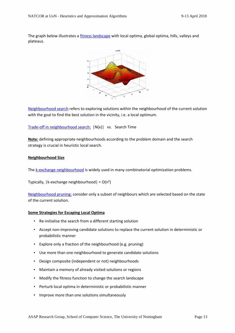
The graph below illustrates a fitness landscape with local optima, global optima, hills, valleys and plateaus.

Neighbourhood search refers to exploring solutions within the neighbourhood of the current solution

with the goal to find the best solution in the vicinity, i.e. a local optimum.

Trade-off in neighbourhood search: |N(x)| vs. Search Time

Note: defining appropriate neighbourhoods according to the problem domain and the search

strategy is crucial in heuristic local search.

Neighbourhood Size

The k-exchange neighbourhood is widely used in many combinatorial optimization problems.

Typically, |k-exchange neighbourhood| = O(nk)

Neighbourhood pruning: consider only a subset of neighbours which are selected based on the state

of the current solution.

Some Strategies for Escaping Local Optima

• Re-initialise the search from a different starting solution

• Accept non-improving candidate solutions to replace the current solution in deterministic or

probabilistic manner

• Explore only a fraction of the neighbourhood (e.g. pruning)

• Use more than one neighbourhood to generate candidate solutions

• Design composite (independent or not) neighbourhoods

• Maintain a memory of already visited solutions or regions

• Modify the fitness function to change the search landscape

• Perturb local optima in deterministic or probabilistic manner

• Improve more than one solutions simultaneously



2.7 Basics of Meta-heuristics

Further preliminary reading: http://www.scholarpedia.org/article/Metaheuristics

Greedy heuristics and simple local search have some limitations with respect to the quality of the

solution that they can produce.

A good balance between intensification and diversification is crucial in order to obtain high-quality

solutions for difficult problems.

A meta-heuristic can be defined as “an iterative master process that guides and modifies the

operations of subordinate heuristics to efficiently produce high-quality solutions. It may manipulate a

complete (or incomplete) single solution or a collection of solutions at each iteration. The

subordinate heuristics may be high (or low) level procedures, or a simple local search, or just a

construction method”(Voss et al. 1999).

A meta-heuristic method is meant to provide a generalized approach that can be applied to different

problems. Meta-heuristics do not need a formal mathematical model of the problem to solve.

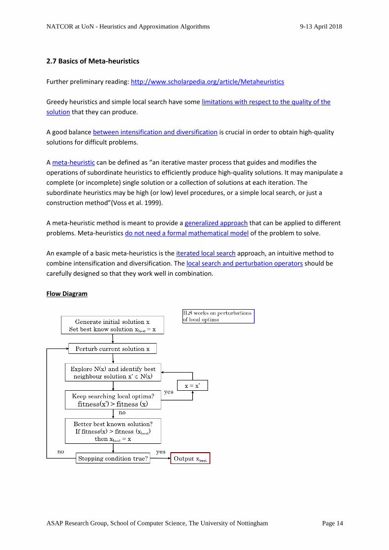
An example of a basic meta-heuristics is the iterated local search approach, an intuitive method to

combine intensification and diversification. The local search and perturbation operators should be

carefully designed so that they work well in combination.

Flow Diagram

http://www.scholarpedia.org/article/Metaheuristics



Some Types of Meta-heuristics

Single-solution method vs. Population-based methods

Nature-inspired method vs. Non-nature inspired methods

‘Pure’ methods vs. Hybrid methods

Memory-based vs. Memory-less methods

Deterministic vs. Stochastic methods

Iterative vs. Greedy methods

The following algorithms are examples of meta-heuristics:

− Iterated local search

− Threshold acceptance

− Great deluge

− Simulated annealing

− Greedy randomised search procedure

− Guided local search

− Variable neighbourhood search

− Tabu search

− Evolutionary algorithms

− Particle swarm optimization

− Artificial immune systems

− Etc.

2.8 Basics of Evolutionary Algorithms

The rationale for evolutionary algorithms (EAs) is to maintain a population of solutions during the

search. The solution (individuals) compete between them and are subject to selection, and

reproduction operators during a number of generations.

Exploitation vs. Exploration

• Having many solutions instead of only one.

• Survival of the fittest principle.

• Pass on good solution components through recombination.

• Explore and discover new components through self-adaptation.

• Solutions are modified from generation to generation by means of reproduction operators

(recombination and self-adaptation).



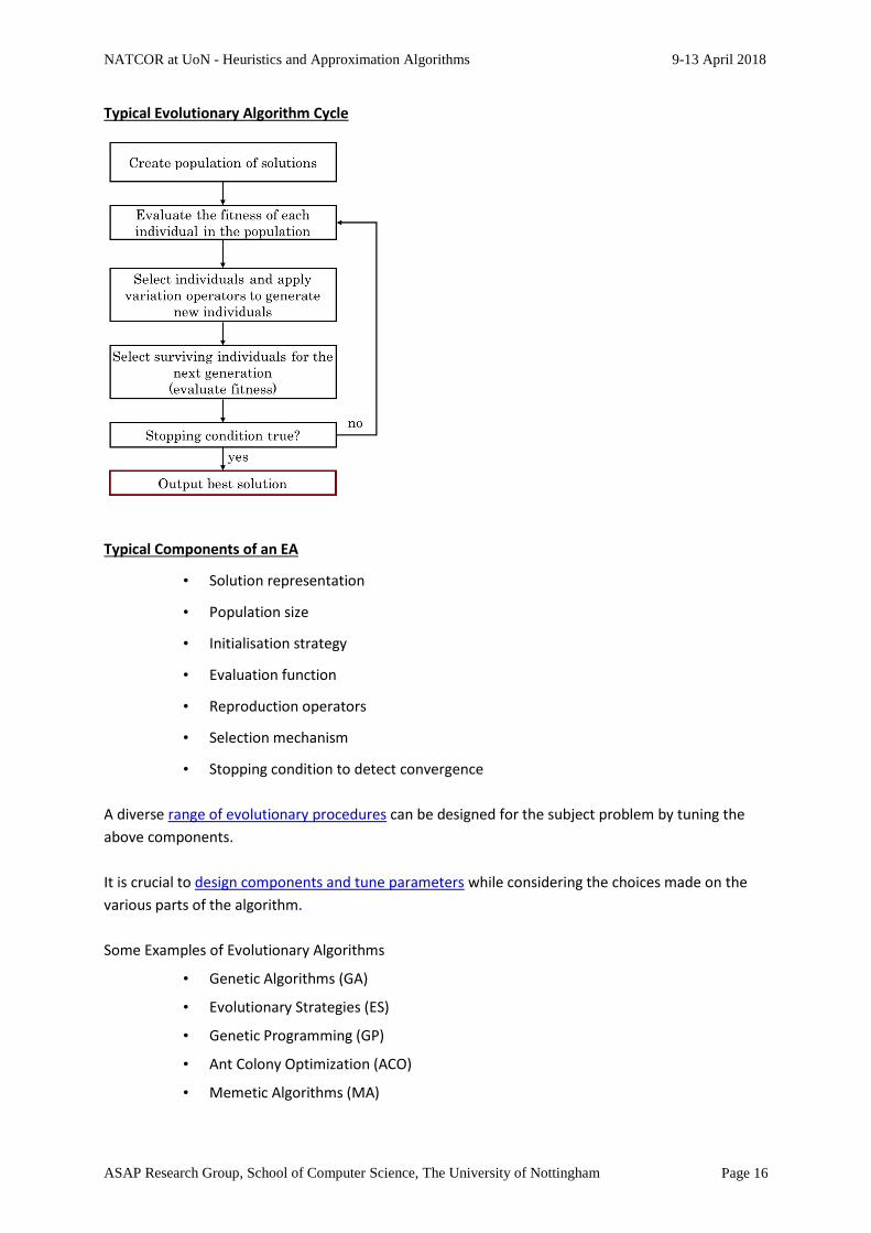
Typical Evolutionary Algorithm Cycle

Typical Components of an EA

• Solution representation

• Population size

• Initialisation strategy

• Evaluation function

• Reproduction operators

• Selection mechanism

• Stopping condition to detect convergence

A diverse range of evolutionary procedures can be designed for the subject problem by tuning the

above components.

It is crucial to design components and tune parameters while considering the choices made on the

various parts of the algorithm.

Some Examples of Evolutionary Algorithms

• Genetic Algorithms (GA)

• Evolutionary Strategies (ES)

• Genetic Programming (GP)

• Ant Colony Optimization (ACO)

• Memetic Algorithms (MA)



• Particle Swarm Optimization (PSO)

• Differential Evolution (DE)

• Estimation of Distribution Algorithm (EDA)

• Cultural Algorithms (CA) Since this a very active research area, new variants of EAs and other population-based meta-

heuristics are often proposed in the specialised literature.

In optimization problems the goal is to find the best feasible solution.

Issues When Dealing with Infeasible Solutions

• Evaluate quality of feasible and infeasible solutions

• Discriminate between feasible and infeasible solutions

• Decide if infeasibility should be eliminated

• Decide if infeasibility should be repaired

• Decide if infeasibility should be penalised

• Initiate the search with feasible solutions, infeasible ones or both

• Maintain feasibility with specialised representations, moves and operators

• Design a decoder to translate an encoding into a feasible solution

• Focus the search on specific areas, e.g. in the boundaries

A constraint handling technique is required to help the effective and efficient exploration of the

search space.

Documents

Pre-requisite Material for Course Heuristics and ... · Pre-requisite Material for Course ... Basics of Heuristic Search for Optimization 7 2.1. Optimization Problems 7 2.2. Linear