Embed Size (px)
Citation preview
Final Research Report Contract T2695, Task 53
Bridge Rapid Construction
Precast Concrete Pier Systems for Rapid Construction of Bridges in Seismic Regions
by
David G. Hieber Graduate Research Assistant
Marc O. Eberhard
Professor
Jonathan M. Wacker Graduate Research Assistant
John F. Stanton
ProfessorDepartment of Civil and Environmental Engineering
University of Washington Seattle, Washington 98195
Washington State Transportation Center (TRAC)
University of Washington, Box 354802 1107 NE 45th Street, Suite 535
Seattle, Washington 98105-4631
Washington State Department of Transportation Technical Monitor
Jugesh Kapur Bridge Design Engineer, Bridge and Structures Office
Prepared for Washington State Transportation Commission
Department of Transportation and in cooperation with
U.S. Department of Transportation Federal Highway Administration
December 2005
TECHNICAL REPORT STANDARD TITLE PAGE 1. REPORT NO. 2. GOVERNMENT ACCESSION NO. 3. RECIPIENT'S CATALOG NO.
WA-RD 611.1
4. TITLE AND SUBTITLE 5. REPORT DATE
PRECAST CONCRETE PIER SYSTEMS FOR RAPID December 2005 CONSTRUCTION OF BRIDGES IN SEISMIC REGIONS 6. PERFORMING ORGANIZATION CODE 7. AUTHOR(S) 8. PERFORMING ORGANIZATION REPORT NO.
David G. Hieber, Jonathan M. Wacker, Marc O. Eberhard John F. Stanton
9. PERFORMING ORGANIZATION NAME AND ADDRESS 10. WORK UNIT NO.
Washington State Transportation Center (TRAC) University of Washington, Box 354802 11. CONTRACT OR GRANT NO.
University District Building; 1107 NE 45th Street, Suite 535 Agreement T2695, Task 53 Seattle, Washington 98105-4631 12. SPONSORING AGENCY NAME AND ADDRESS 13. TYPE OF REPORT AND PERIOD COVERED
Research Office Washington State Department of Transportation Transportation Building, MS 47372
Final Research Report
Olympia, Washington 98504-7372 14. SPONSORING AGENCY CODE
Kim Willoughby, Project Manager, 360-705-7978 15. SUPPLEMENTARY NOTES
This study was conducted in cooperation with the U.S. Department of Transportation, Federal Highway Administration. 16. ABSTRACT
Increasing traffic volumes and a deteriorating transportation infrastructure have stimulated the development of new systems and methods to accelerate the construction of highway bridges. Precast concrete bridge components offer a potential alternative to conventional reinforced, cast-in-place concrete components. The use of precast components has the potential to minimize traffic disruptions, improve work zone safety, reduce environmental impacts, improve constructability, increase quality, and lower life-cycle costs.
This study compared two precast concrete bridge pier systems for rapid construction of bridges in seismic regions. One was a reinforced concrete system, in which mild steel deformed bars connect the precast concrete components. The other was a hybrid system, which uses a combination of unbonded post-tensioning and mild steel deformed bars to make the connections.
A parametric study was conducted using nonlinear finite element models to investigate the global response and likelihood of damage for various configurations of the two systems subjected to a design level earthquake. A practical method was developed to estimate the maximum seismic displacement of a frame from the cracked section properties of the columns and the base-shear strength ratio.
The results of the parametric study suggest that the systems have the potential for good seismic performance. Further analytical and experimental research is needed to investigate the constructability and seismic performance of the connection details. 17. KEY WORDS 18. DISTRIBUTION STATEMENT
Bridges, piers, substructures, rapid construction, seismic performance, connections, precast concrete, prestressed concrete
No restrictions. This document is available to the public through the National Technical Information Service, Springfield, VA 22616
19. SECURITY CLASSIF. (of this report) 20. SECURITY CLASSIF. (of this page) 21. NO. OF PAGES 22. PRICE
None None

DISCLAIMER
The contents of this report reflect the views of the authors, who are responsible
for the facts and the accuracy of the data presented herein. The contents do not
necessarily reflect the official views or policies of the Washington State Transportation
Commission, Department of Transportation, or the Federal Highway Administration.
This report does not constitute a standard, specification, or regulation.
iii

iv
TABLE OF CONTENTS
EXECUTIVE SUMMARY .......................................................................................... xvii CHAPTER 1 INTRODUCTION......................................................................................1 1.1 Benefits of Rapid Construction.......................................................................2 1.1.1 Reduced Traffic Disruption ...................................................................2 1.1.2 Improved Work Zone Safety .................................................................3 1.1.3 Reduced Environmental Impact.............................................................4 1.1.4 Improved Constructability .....................................................................4 1.1.5 Increased Quality ...................................................................................5 1.1.6 Lower Life-Cycle Costs.........................................................................5 1.2 Research Objectives........................................................................................5 1.3 Scope of Research...........................................................................................6 1.4 Report Organization........................................................................................8 CHAPTER 2 PREVIOUS RESEARCH ........................................................................10 2.1 Precast Concrete Pier Components for Non-Seismic Regions .....................11 2.2 Precast Concrete Building Components for Seismic Regions......................13 2.3 Precast Concrete Pier Components for Seismic Regions .............................14 CHAPTER 3 PROPOSED PRECAST SYSTEMS.......................................................16 3.1 Reinforced Concrete System.........................................................................18 3.1.1 System Description ..............................................................................18 3.1.2 Proposed Construction Sequence.........................................................20 3.1.3 Column-to-Column Connections .........................................................28 3.2 Hybrid System ..............................................................................................34 3.2.1 System Description ..............................................................................35 3.2.2 Proposed Construction Sequence.........................................................37 3.2.3 Details of Column-to-Cap-Beam Connections ....................................43 CHAPTER 4 ANALYTICAL MODEL.........................................................................47 4.1 Prototype Bridge ...........................................................................................48 4.2 Baseline Frames ............................................................................................50 4.3 Column Characteristics.................................................................................54 4.4 Cap-Beam Characteristics.............................................................................59 4.5 Joint Characteristics ......................................................................................59 4.6 Methodology for Pushover Analyses............................................................60 4.7 Methodology for Earthquake Analyses ........................................................61 CHAPTER 5 SELECTION OF GROUND MOTIONS...............................................63 5.1 Selection of Seismic Hazard Level ...............................................................64 5.2 Ground Motion Database..............................................................................65 5.3 Acceleration Response Spectrum .................................................................66
v
5.4 Design Acceleration Response Spectrum .....................................................67 5.5 Scaling of Ground Motions...........................................................................69 5.6 Selection of Ground Motions........................................................................70 CHAPTER 6 PUSHOVER ANALYSES OF REINFORCED CONCRETE
FRAMES...............................................................................................................75 6.1 Range of Reinforced Concrete Parametric Study .........................................75 6.1.1 Column Aspect Ratio, col colL D ..........................................................78 6.1.2 Longitudinal Reinforcement Ratio, ρ ................................................78 6.1.3 Axial-Load Ratio, '(col c gP f A ) ............................................................79 6.1.4 Frame Designation ...............................................................................79 6.2 Key Characteristics of Pushover Response...................................................79 6.2.1 Uncracked Properties ...........................................................................80 6.2.2 First Yield ............................................................................................80 6.2.3 Cracked Properties ...............................................................................81 6.2.4 Stiffness Ratio, cracked uncrackedk k ...........................................................82 6.2.5 Effective Force at Concrete Strain of 0.004, ............................82 004conF 6.2.6 Nominal Yield Displacement, yΔ .......................................................82 6.2.7 Maximum Force, .........................................................................83 maxF 6.3 Trends in Stiffness Ratio...............................................................................83 6.4 Trends in Nominal Yield Displacements......................................................87 6.5 Trends in Maximum Force............................................................................90 CHAPTER 7 EARTHQUAKE ANALYSES OF REINFORCED CONCRETE FRAMES......................................................................................................93 7.1 Range of Reinforced Concrete Parametric Study .........................................93 7.2 Key Characteristics of Earthquake Response ...............................................94 7.2.1 Maximum Displacement, maxΔ ............................................................94 7.2.2 Residual Displacement, residualΔ ...........................................................94 7.3 Trends in Maximum Displacement...............................................................95 7.4 Effects of Strength on Maximum Displacement...........................................99 7.5 Comparison of Maximum Displacement with Elastic Analysis .................104 7.6 Incorporation of Strength in Prediction of Maximum Displacement .........108 7.7 Trends in Residual Displacement ...............................................................110 CHAPTER 8 PUSHOVER ANALYSES OF HYBRID FRAMES............................114 8.1 Range of Hybrid Parametric Study .............................................................114 8.1.1 Column Aspect Ratio, col colL D ........................................................115 8.1.2 Axial-Load Ratio, '(col c gP f A ) ..........................................................115 8.1.3 Equivalent Reinforcement Ratio........................................................116 8.1.4 Re-centering Ratio, rcλ ......................................................................116 8.1.5 Frame Designation .............................................................................117 8.1.6 Practical Frame Combinations...........................................................118
vi
8.2 Key Characteristics of Pushover Response.................................................121 8.2.1 Uncracked Properties .........................................................................121 8.2.2 First Yield ..........................................................................................122 8.2.3 Cracked Properties .............................................................................123 8.2.4 Stiffness Ratio, cracked uncrackedk k .........................................................123 8.2.5 Effective Force at a Concrete Strain of 0.004, .......................123 004conF 8.2.6 Nominal Yield Displacement, yΔ .....................................................123 8.2.7 Maximum Force, .......................................................................124 maxF 8.3 Trends in Stiffness Ratio.............................................................................124 8.4 Trends in Nominal Yield Displacements....................................................130 8.5 Trends in Maximum Force..........................................................................135 CHAPTER 9 EARTHQUAKE ANALYSES OF HYBRID FRAMES .....................139 9.1 Range of Hybrid Parametric Study .............................................................139 9.2 Key Characteristics of Earthquake Response .............................................139 9.2.1 Maximum Displacement, maxΔ ..........................................................140 9.2.2 Residual Displacement, residualΔ .........................................................140 9.3 Trends in Maximum Displacement.............................................................141 9.4 Effects of Strength on Maximum Displacement.........................................149 9.5 Comparison of Maximum Displacement with Elastic Analysis .................155 9.6 Incorporation of Strength in Prediction of Maximum Displacement .........160 9.7 Trends in Residual Displacement ...............................................................162 CHAPTER 10 SEISMIC PERFORMANCE EVALUATION ..................................164 10.1 Displacement Ductility Demand.................................................................167 10.2 Onset of Cover Concrete Spalling ..............................................................174 10.3 Onset of Bar Buckling ................................................................................183 10.4 Maximum Strain in Longitudinal Mild Steel..............................................190 10.5 Proximity to Ultimate Displacement ..........................................................197 10.6 Sensitivity of Performance to Frame Parameters........................................204 CHAPTER 11 SUMMARY, CONCLUSIONS, AND RECOMMENDATIONS.....210 11.1 Summary .....................................................................................................210 11.2 Conclusions from System Development.....................................................212 11.3 Conclusions from the Pushover Analyses...................................................213 11.4 Conclusions from the Earthquake Analyses ...............................................214 11.5 Conclusions from the Seismic Performance Evaluation.............................216 11.6 Recommendations for Further Study ..........................................................218 ACKNOWLEDGMENTS .............................................................................................221 REFERENCES...............................................................................................................222 APPENDIX A: GROUND MOTION CHARACTERISTICS.................................. A-1
vii

APPENDIX B: RESULTS FROM EARTHQUAKE ANALYSES OF REINFORCED CONCRETE FRAMES ................................................B-1 APPENDIX C: RESULTS FROM EARTHQUAKE ANALYSES OF HYBRID
FRAMES............................................................................................................ C-1 APPENDIX D: DETAILS OF SEISMIC PERFORMANCE EVALUATION....... D-1
viii
LIST OF FIGURES
Figure Page 3.1: Elevation of Reinforced Concrete System Pier ..................................................19 3.2: Expected Behavior of the Connection in Reinforced Concrete Frames .............20 3.3: Proposed Construction Sequence for Reinforced Concrete Frames ...................21 3.4: Proposed Footing-to-Column Connection for Reinforced Concrete Frames .....23 3.5: Precast Column for Reinforced Concrete Frames ..............................................24 3.6: Cap-Beam Details for Slotted Opening Connection for Reinforced
Concrete Frames .................................................................................................29 3.7: Column and Cap-Beam for Slotted Opening Connection for Reinforced
Concrete Frames .................................................................................................30 3.8: Cap-Beam Details for Complete Opening Connection for Reinforced
Concrete Frames .................................................................................................33 3.9: Column and Cap-Beam for Complete Opening Connection for Reinforced
Concrete Frames .................................................................................................34 3.10: Elevation of Hybrid System Pier ........................................................................35 3.11: Expected Behavior of the Connection in Hybrid Frames ...................................37 3.12: Proposed Construction Sequence for Hybrid Frames.........................................38 3.13: Proposed Footing-to-Column Connection for Hybrid Frames ...........................39 3.14: Precast Column for Hybrid Frames ....................................................................41 3.15: Cap-Beam Details for Individual Splice Sleeve Connection for Hybrid
Frames.................................................................................................................45 3.16: Column and Cap-Beam for Individual Splice Sleeve Connection for Hybrid Frames ....................................................................................................46 4.1: Typical Elevation of Reinforced Concrete Pier ..................................................49 4.2: Elevation of Reinforced Concrete Baseline Frame.............................................51 4.3: Elevation of Hybrid Baseline Frame...................................................................52 5.1: Acceleration Response Spectrum (Ground Motion 10-1) ..................................67 5.2: 10 Percent in 50 and 2 Percent in 50 Design Acceleration Response
Spectrum .............................................................................................................69 5.3: Example of Ground Motion Characteristics (Ground Motion 10-1) ..................73 5.4: Average 10 Percent in 50 Acceleration Response Spectrum and 10 Percent
in 50 Design Acceleration Response Spectrum..................................................74 5.5: Average 2 Percent in 50 Acceleration Response Spectrum and 2 Percent in
50 Design Acceleration Response Spectrum ......................................................74 6.1: Effect of Column Diameter on Pushover Response ...........................................77 6.2: Idealized Force-Displacement Curve..................................................................81 6.3: Stiffness Ratio, Reinforced Concrete Frames.....................................................85 6.4: Yield Displacement, Reinforced Concrete Frames.............................................89 6.5: Maximum Force, Reinforced Concrete Frames..................................................91
ix

7.1: Trends in Drift Ratio, 2 Percent in 50, Reinforced Concrete Frames.................97 7.2: Effect of Strength on Mean Drift Ratio, 2 Percent in 50, Reinforced
Concrete Frames ...............................................................................................100 7.3: Effect of Strength on Mean Plus One Standard Deviation Drift Ratio, 2 Percent in 50, Reinforced Concrete Frames ..................................................101 7.4: 10 Percent in 50 Design Displacement Response Spectrum ............................102 7.5: Effect of Stiffness on Mean Drift Ratio, 2 Percent in 50, Reinforced
Concrete Frames ...............................................................................................103 7.6: Effect of Stiffness on Mean Plus One Standard Deviation Drift Ratio, 2 Percent in 50, Reinforced Concrete Frames ..................................................104 7.7: Predicted and Mean Response, 2 Percent in 50, Reinforced Concrete Frames 106 7.8: Predicted and Mean Plus One Standard Deviation Response, 2 Percent in
50, Reinforced Concrete Frames.......................................................................107 7.9: Bilinear Approximation for Maximum Displacement......................................109 7.10: Effects of Damping Ratio and SHR on Residual Drift .....................................112 8.1: Idealized Force-Displacement Curve................................................................122 8.2: Stiffness Ratio, Hybrid Frames, '( ) 0.05col c gP f A = .........................................127
8.3: Stiffness Ratio, Hybrid Frames, '( ) 0.10col c gP f A = .........................................128
8.4: Yield Displacement, Hybrid Frames, '( ) 0.05col c gP f A = .................................132
8.5: Yield Displacement, Hybrid Frames, '( ) 0.10col c gP f A = .................................133
8.6: Maximum Force, Hybrid Frames, '( ) 0.05col c gP f A = ......................................136
8.7: Maximum Force, Hybrid Frames, '( ) 0.10col c gP f A = ......................................137 9.1: Trends in Drift Ratio, 2 Percent in 50, Hybrid Frames, '( ) 0.05col c gP f A = .....143
9.2: Trends in Drift Ratio, 2 Percent in 50, Hybrid Frames, '( ) 0.10col c gP f A = .....144
9.3: Effect of Steel Ratio, 2 Percent in 50, Hybrid Frames, '( ) 0.05col c gP f A = ......145
9.4: Effect of Steel Ratio, 2 Percent in 50, Hybrid Frames, '( ) 0.10col c gP f A = ......146 9.5: Effect of Strength on Mean Drift Ratio, 2 Percent in 50, Hybrid Frames,
'( ) 0.05col c gP f A = .............................................................................................150 9.6: Effect of Strength on Mean Plus One Standard Deviation Drift Ratio, 2 Percent in 50, Hybrid Frames, '( ) 0.05col c gP f A = ........................................151 9.7: Effect of Strength on Mean Drift Ratio, 2 Percent in 50, Hybrid Frames,
'( ) 0.10col c gP f A = .............................................................................................151 9.8: Effect of Strength on Mean Plus One Standard Deviation Drift Ratio, 2 Percent in 50, Hybrid Frames, '( ) 0.10col c gP f A = ........................................152 9.9: Effect of Stiffness on Mean Drift Ratio, 2 Percent in 50, Hybrid Frames,
'( ) 0.05col c gP f A = .............................................................................................153 9.10: Effect of Stiffness on Mean Plus One Standard Deviation Drift Ratio,
x
2 Percent in 50, Hybrid Frames, '( ) 0.05col c gP f A = ........................................154 9.11: Effect of Stiffness on Mean Drift Ratio, 2 Percent in 50, Hybrid Frames,
'( ) 0.10col c gP f A = .............................................................................................154 9.12: Effect of Stiffness on Mean Plus One Standard Deviation Drift Ratio, 2 Percent in 50, Hybrid Frames, '( ) 0.10col c gP f A = ........................................155 9.13: Predicted and Mean Response, 2 Percent in 50, Hybrid Frames,
'( ) 0.05col c gP f A = .............................................................................................158 9.14: Predicted and Mean Plus One Standard Deviation Response, 2 Percent in 50, Hybrid Frames, '( ) 0.05col c gP f A = ..................................................................158 9.15: Predicted and Mean Response, 2 Percent in 50, Hybrid Frames,
'( ) 0.10col c gP f A = .............................................................................................159 9.16: Predicted and Mean Plus One Standard Deviation Response, 2 Percent in 50, Hybrid Frames, '( ) 0.10col c gP f A = ..................................................................159 9.17: Bilinear Approximation for Maximum Displacement......................................161 10.1: Displacement Ductility, 2 Percent in 50, Reinforced Concrete Frames ...........169 10.2: Displacement Ductility, 2 Percent in 50, Hybrid Frames, '( ) 0.05col c gP f A = .170
10.3: Displacement Ductility, 2 Percent in 50, Hybrid Frames, '( ) 0.10col c gP f A = .171 10.4: Cover Spalling, 2 Percent in 50, Reinforced Concrete Frames ........................178 10.5: Cover Spalling, 2 Percent in 50, Hybrid Frames, '( ) 0.05col c gP f A = ..............179
10.6: Cover Spalling, 2 Percent in 50, Hybrid Frames, '( ) 0.10col c gP f A = ..............180 10.7: Bar Buckling, 2 Percent in 50, Reinforced Concrete Frames ...........................186 10.8: Bar Buckling, 2 Percent in 50, Hybrid Frames, '( ) 0.05col c gP f A = .................187
10.9: Bar Buckling, 2 Percent in 50, Hybrid Frames, '( ) 0.10col c gP f A = .................188 10.10: Maximum Steel Strain, 2 Percent in 50, Reinforced Concrete Frames ............193 10.11: Maximum Steel Strain, 2 Percent in 50, Hybrid Frames, '( ) 0.05col c gP f A = ..194
10.12: Maximum Steel Strain, 2 Percent in 50, Hybrid Frames, '( ) 0.10col c gP f A = ..195 10.13: max ultΔ Δ , 2 Percent in 50, Reinforced Concrete Frames ................................200 10.14: max ultΔ Δ , 2 Percent in 50, Hybrid Frames, '( ) 0.05col c gP f A = ......................201
10.15: max ultΔ Δ , 2 Percent in 50, Hybrid Frames, '( ) 0.10col c gP f A = ......................202 A.1: Characteristics of Ground Motion 10-1 ........................................................... A-2 A.2: Characteristics of Ground Motion 10-2 ........................................................... A-3 A.3: Characteristics of Ground Motion 10-3 ........................................................... A-4 A.4: Characteristics of Ground Motion 10-4 ........................................................... A-5 A.5: Characteristics of Ground Motion 10-5 ........................................................... A-6 A.6: Characteristics of Ground Motion 2-1 ............................................................. A-7 A.7: Characteristics of Ground Motion 2-2 ............................................................. A-8 A.8: Characteristics of Ground Motion 2-3 ............................................................. A-9
xi
A.9: Characteristics of Ground Motion 2-4 ........................................................... A-10 A.10: Characteristics of Ground Motion 2-5 ........................................................... A-11 B.1: Trends in Drift Ratio, 10 Percent in 50, Reinforced Concrete Frames.............B-4 B.2: Effect of Strength on Mean Drift Ratio, 10 Percent in 50, Reinforced
Concrete Frames ...............................................................................................B-5 B.3: Effect of Strength on Mean Plus One Standard Deviation Drift Ratio, 10 Percent in 50, Reinforced Concrete Frames ................................................B-5 B.4: Effect of Stiffness on Mean Drift Ratio, 10 Percent in 50, Reinforced Concrete Frames ...............................................................................................B-6 B.5: Effect of Stiffness on Mean Plus One Standard Deviation Drift Ratio, 10 Percent in 50, Reinforced Concrete Frames ................................................B-6 B.6: Predicted and Mean Response, 10 Percent in 50, Reinforced Concrete
Frames...............................................................................................................B-7 B.7: Predicted and Mean Plus One Standard Deviation Response, 10 Percent in
50, Reinforced Concrete Frames.......................................................................B-7 C.1: Trends in Drift Ratio, 10 Percent in 50, Hybrid Frames, '( ) 0.05col c gP f A = ...C-4
C.2: Trends in Drift Ratio, 10 Percent in 50, Hybrid Frames, '( ) 0.10col c gP f A = ...C-5
C.3: Effect of Steel Ratio, 10 Percent in 50, Hybrid Frames, '( ) 0.05col c gP f A = ....C-6
C.4: Effect of Steel Ratio, 10 Percent in 50, Hybrid Frames, '( ) 0.10col c gP f A = ....C-7 C.5: Effect of Strength on Mean Drift Ratio, 10 Percent .........................................C-8 C.6: Effect of Strength on Mean Plus One Standard Deviation Drift Ratio, 10 Percent in 50, Hybrid Frames, '( ) 0.05col c gP f A = ......................................C-8 C.7: Effect of Strength on Mean Drift Ratio, 10 Percent in 50, Hybrid Frames,
'( ) 0.10col c gP f A = .............................................................................................C-9 C.8: Effect of Strength on Mean Plus One Standard Deviation Drift Ratio, 10 Percent in 50, Hybrid Frames, '( ) 0.10col c gP f A = ......................................C-9 C.9: Effect of Stiffness on Mean Drift Ratio, 10 Percent in 50, Hybrid Frames,
'( ) 0.05col c gP f A = ...........................................................................................C-10 C.10: Effect of Stiffness on Mean Plus One Standard Deviation Drift Ratio, 10 Percent in 50, Hybrid Frames, '( ) 0.05col c gP f A = ....................................C-10 C.11: Effect of Stiffness on Mean Drift Ratio, 10 Percent in 50, Hybrid Frames,
'( ) 0.10col c gP f A = ...........................................................................................C-11 C.12: Effect of Stiffness on Mean Plus One Standard Deviation Drift Ratio, 10 Percent in 50, Hybrid Frames, '( ) 0.10col c gP f A = ....................................C-11 C.13: Predicted and Mean Response, 10 Percent in 50, Hybrid Frames,
'( ) 0.05col c gP f A = ...........................................................................................C-12 C.14: Predicted and Mean Plus One Standard Deviation Response, 10 Percent in
50, Hybrid Frames, '( ) 0.05col c gP f A = ..........................................................C-12
xii
C.15: Predicted and Mean Response, 10 Percent in 50, Hybrid Frames, '( ) 0.10col c gP f A = ...........................................................................................C-13
C.16: Predicted and Mean Plus One Standard Deviation Response, 10 Percent in 50, Hybrid Frames, '( ) 0.10col c gP f A = ..........................................................C-13
D.1: Displacement Ductility, 10 Percent in 50, Reinforced Concrete Frames ...... D-12 D.2: Displacement Ductility, 10 Percent in 50, Hybrid Frames,
'( ) 0.05col c gP f A = D-13 D.3: Displacement Ductility, 10 Percent in 50, Hybrid Frames,
'( ) 0.10col c gP f A = .......................................................................................... D-14 D.4: Cover Spalling, 10 Percent in 50, Reinforced Concrete Frames ................... D-15 D.5: Cover Spalling, 10 Percent in 50, Hybrid Frames, '( ) 0.05col c gP f A = ......... D-16
D.6: Cover Spalling, 10 Percent in 50, Hybrid Frames, '( ) 0.10col c gP f A = ......... D-17 D.7: Bar Buckling, 10 Percent in 50, Reinforced Concrete Frames ...................... D-18 D.8: Bar Buckling, 10 Percent in 50, Hybrid Frames, '( ) 0.05col c gP f A = ............ D-19
D.9: Bar Buckling, 10 Percent in 50, Hybrid Frames, '( ) 0.10col c gP f A = ............ D-20 D.10: Maximum Steel Strain, 10 Percent in 50, Reinforced Concrete Frames ....... D-21 D.11: Maximum Steel Strain, 10 Percent in 50, Hybrid Frames,
'( ) 0.05col c gP f A = .......................................................................................... D-22 D.12: Maximum Steel Strain, 10 Percent in 50, Hybrid Frames,
'( ) 0.10col c gP f A = .......................................................................................... D-23 D.13: max ultΔ Δ , 10 Percent in 50, Reinforced Concrete Frames ........................... D-24 D.14: max ultΔ Δ , 10 Percent in 50, Hybrid Frames, '( ) 0.05col c gP f A = ................. D-25
D.15: max ultΔ Δ , 10 Percent in 50, Hybrid Frames, '( ) 0.10col c gP f A = ................. D-26
xiii
LIST OF TABLES Table Page 5.1: Final Ground Motion Suite .................................................................................72 6.1: Natural Periods and Stiffnesses, Reinforced Concrete Frames ..........................83 6.2: Yield and Strength Properties, Reinforced Concrete Frames .............................87 7.1: Effect of Damping Ratio and SHR on Residual Displacement ........................112 8.1: Reinforcing Properties, Hybrid Frames, ( )' 0.05col c gP f A = .............................120
8.2: Reinforcing Properties, Hybrid Frames, ( )' 0.10col c gP f A = .............................121
8.3: Natural Periods and Stiffnesses, Hybrid Frames, ( )' 0.05col c gP f A = ..............125
8.4: Natural Periods and Stiffnesses, Hybrid Frames, ( )' 0.10col c gP f A = ..............126
8.5: Yield and Strength Properties, Hybrid Frames, ( )' 0.05col c gP f A = .................130
8.6: Yield and Strength Properties, Hybrid Frames, ( )' 0.10col c gP f A = .................131 10.1: Comparison of Performance of Reinforced Concrete and Hybrid Frames.......205 10.2: Sensitivity of Performance, Reinforced Concrete Frames................................207 10.3: Sensitivity of Performance, Hybrid Frames......................................................208 B.1: Maximum Displacements, 10 Percent in 50, Reinforced Concrete Frames .....B-2 B.2: Maximum Displacements, 2 Percent in 50, Reinforced Concrete Frames .......B-3 C.1: Maximum Displacements, 10 Percent in 50, Hybrid Frames,
( )' 0.05col c gP f A = ............................................................................................C-2 C.2: Maximum Displacements, 10 Percent in 50, Hybrid Frames,
( )' 0.10col c gP f A = ............................................................................................C-2 C.3: Maximum Displacements, 2 Percent in 50, Hybrid Frames,
( )' 0.05col c gP f A = ............................................................................................C-3 C.4: Maximum Displacements, 2 Percent in 50, Hybrid Frames,
( )' 0.10col c gP f A = ............................................................................................C-3 D.1 Displacement Ductility Demand, Reinforced Concrete Frames...................... D-2 D.2 Displacement Ductility Demand, Hybrid Frames, ( )' 0.05col c gP f A = ........... D-3
D.3 Displacement Ductility Demand, Hybrid Frames, ( )' 0.10col c gP f A = ........... D-3 D.4 Probability of Cover Spalling, Reinforced Concrete Frames .......................... D-4
xiv
D.5 Probability of Cover Spalling, Hybrid Frames, ( )' 0.05col c gP f A = ................ D-5
D.6 Probability of Cover Spalling, Hybrid Frames, ( )' 0.10col c gP f A = ................ D-5 D.7 Probability of Bar Buckling, Reinforced Concrete Frames ............................. D-6 D.8 Probability of Bar Buckling, Hybrid Frames, ( )' 0.05col c gP f A = .................. D-7
D.9 Probability of Bar Buckling, Hybrid Frames, ( )' 0.10col c gP f A = .................. D-7 D.10 Maximum Steel Strain, Reinforced Concrete Frames ..................................... D-8 D.11 Maximum Steel Strain, Hybrid Frames, ( )' 0.05col c gP f A = ........................... D-9
D.12 Maximum Steel Strain, Hybrid Frames, ( )' 0.10col c gP f A = ........................... D-9
D.13 max ultΔ Δ , Reinforced Concrete Frames........................................................ D-10
D.14 max ultΔ Δ , Hybrid Frames, ( )' 0.05col c gP f A = ............................................. D-11
D.15 max ultΔ Δ , Hybrid Frames, ( )' 0.10col c gP f A = ............................................. D-11
xv

xvi
EXECUTIVE SUMMARY
Increasing traffic volumes and a deteriorating transportation infrastructure have
stimulated the development of new systems and methods to accelerate the construction of
highway bridges in order to reduce traveler delays. Precast concrete bridge components
offer a potential alternative to conventional reinforced, cast-in-place concrete
components. The increased use of precast concrete components could facilitate rapid
construction, minimize traffic disruption, improve work zone safety, reduce
environmental impacts, improve constructability, and lower life-cycle costs. .
This study compared two precast concrete bridge pier systems for rapid
construction of bridges in seismic regions. The systems made use of precast concrete
cap-beams and columns supported on cast-in-place concrete foundations. One was a
reinforced concrete system, in which mild steel deformed bars connected the precast
concrete components and provided the flexural strength of the columns. The other was a
hybrid system, which used a combination of unbonded post-tensioning and mild steel
deformed bars to make the connections and provide the required flexural stiffness and
strength.
A parametric study of the two systems, which included pushover and earthquake
analyses of 36 reinforced concrete frames and 57 hybrid frames, was conducted using
nonlinear finite element models to investigate the global response of various frame
configurations. In the earthquake analyses, the frames were subjected to five ground
motions having peak ground accelerations with a 10 percent probability of exceedance in
50 years (10 percent in 50) and five ground motions having peak ground accelerations
xvii
with a 2 percent probability of exceedance in 50 years (2 percent in 50), resulting in a
total of 930 earthquake analyses.
A practical method was developed to estimate maximum seismic displacements
on the basis of the cracked section properties of the columns and base-shear strength
ratio. The ratio of the maximum displacement calculated with nonlinear analysis to the
displacement calculated with the practical method had a mean of 0.98 and a standard
deviation of 0.25 for the reinforced concrete frames. For the hybrid frames, this ratio had
a mean of 1.05 and a standard deviation of 0.26.
The expected damage at the two seismic hazard levels was estimated. For the 10 percent
in 50 ground motions, this study found moderate probabilities of cover concrete spalling,
minimal probabilities of bar buckling, and maximum strains in the longitudinal
reinforcement that suggest bar fracture would rarely occur. For example, at an axial-load
ratio of 0.10 and longitudinal reinforcement ratio of 0.01, the mean probability of cover
concrete spalling was 0.12 for the reinforced concrete frames and 0.10 for the hybrid
frames, while the mean probability of bar buckling was 0.0005 for both the reinforced
concrete and hybrid frames. For this same axial-load ratio and reinforcement ratio, the
mean maximum strain in the longitudinal mild steel was 0.015 for the reinforced concrete
frames and 0.012 for the hybrid frames.
Large probabilities of cover concrete spalling, minimal probabilities of bar
buckling, and moderate maximum strains in the longitudinal reinforcement were found
for the 2 percent in 50 ground motions. For example, at an axial-load ratio of 0.10 and
longitudinal reinforcement ratio of 0.01, the mean probability of cover concrete spalling
was 0.68 for the reinforced concrete frames and 0.73 for the hybrid frames, while the
xviii

mean probability of bar buckling was 0.04 for the reinforced concrete and hybrid frames.
For this same axial-load ratio and reinforcement ratio, the mean maximum strain in the
longitudinal mild steel was 0.042 for the reinforced concrete frames and 0.025 for the
hybrid frames.
This study found that the hybrid system exhibited particularly low residual drifts.
This study also found the displacement ductility demand of the two systems to be similar
for similar levels of axial-load ratio and total longitudinal reinforcement.
On the basis of the global nonlinear finite element analyses conducted during this
study, the characteristics and numerical response quantities suggest that the systems have
the potential for good seismic performance. Further research is needed to develop the
connection details.
xix

xx
CHAPTER 1 INTRODUCTION
A significant cause of increasing traffic congestion in the Puget Sound Region, as
well as in many other parts of the United States, is that traffic volumes continue to
increase at the same time as the interstate highway system is approaching its service life
(Freeby et al. 2003). To improve the condition of the deteriorating transportation
infrastructure, significant bridge repairs and new bridge construction are necessary.
Unfortunately, even though these solutions help reduce traffic congestion after the
construction or rehabilitation is complete, they typically further increase traffic
congestion during the construction or rehabilitation. Therefore, accelerated construction
methods incorporating new practices, technologies, and systems are needed to facilitate
rapid construction of bridges. The American Association of State Highway and
Transportation Officials (AASHTO), the Federal Highway Administration (FHWA), and
various state departments of transportation have been working together to develop these
systems and methods that would allow for more rapid construction of bridges and other
transportation infrastructure (FHWA 2004).
A majority of the highway bridges currently constructed in Washington State
consist of prestressed concrete girders with a composite, reinforced, cast-in-place
concrete deck slab supported by reinforced, cast-in-place concrete bridge piers and
abutments. Cast-in-place concrete bridge construction significantly contributes to traffic
disruption because it requires numerous, sequential on-site construction procedures and
can be time-intensive.
1
Precast concrete bridge components offer a promising alternative to their cast-in-
place concrete counterparts. Enormous benefits could arise from their use because
precast concrete bridge components are typically fabricated off-site and then brought to
the project site and quickly erected. Precast components also provide an opportunity to
complete tasks in parallel. For example, the foundations can be cast on-site while the
precast components are fabricated off-site. The use of precast components has the
potential to minimize traffic disruptions, improve work zone safety, reduce
environmental impacts, improve constructability, increase quality, and lower life-cycle
costs. The use of precast concrete bridge elements can provide dramatic benefits for
bridge owners, designers, contractors, and the traveling public (Freeby et al. 2003).
Several precast concrete bridge pier systems have been proposed and developed
recently. Some of these are reinforced concrete frames that use mild reinforcing steel
alone to connect the precast concrete components. Others are hybrid frames that use
unbonded, post-tensioning tendons in conjunction with grouted, mild reinforcing steel to
achieve the necessary connection. Precast pier systems have been developed for non-
seismic regions (Billington et al. 1998, Matsumoto et al. 2002). In comparison, the
development of connections between precast concrete components for use in seismic
regions has been limited. Hybrid frames have the additional benefit of minimizing
residual displacement by re-centering the frame after an earthquake.
1.1 BENEFITS OF RAPID CONSTRUCTION
1.1.1 Reduced Traffic Disruption
Construction-related traffic delays are not only frustrating; they can impose
unacceptable delays on the traveling public and for the nation’s commerce. This situation
2
is spurring interest in rapid construction methods. To reduce motorist inconvenience,
lost time, and wasted fuel, some states are beginning to offer contractors bonuses for
using rapid construction methods to complete projects earlier and charging them penalties
for late completion (Ralls and Tang 2004).
Typically, highway bridges are constructed of cast-in-place reinforced concrete
abutments and piers, precast concrete or steel girders, and a cast-in-place reinforced
concrete deck slab. Although these practices generally produce durable bridges, they also
contribute significantly to traffic delays because of the sequential nature of the
construction. Foundations must be formed, poured, and cured before columns and pier
caps can be placed. Columns and pier caps must be formed, poured, and cured before the
girders and deck are placed. A construction schedule needs to include additional time
delays to allow the concrete to cure between each operation (Freeby et al. 2003).
Precast bridge elements and systems allow for many of the tasks traditionally
performed on-site, such as element fabrication, to be performed away from the
construction site and traffic. Precast bridge elements and systems also allow many of the
time-consuming tasks, such as erecting formwork, placing reinforcing steel, pouring
concrete, curing concrete, and removing formwork, to occur off-site (Freeby et al. 2003).
Precast elements can be transported to the site and erected quickly, significantly reducing
the disruption of traffic and the cost of traffic control.
1.1.2 Improved Work Zone Safety
Bridge construction sites often require workers to operate close to high-speed
traffic, at high elevations, over water, near power lines, or in other dangerous situations
(Freeby et al. 2003). Precast elements allow many of the construction activities to occur
3

in a safer, more controlled environment, significantly reducing the amount of time
workers must operate in a potentially dangerous setting.
1.1.3 Reduced Environmental Impact
Precast elements are advantageous for bridges constructed over water, wetlands,
and other sensitive areas, in which environmental concerns and regulations discourage
the use of cast-in-place concrete. Traditional bridge construction requires significant
access underneath the bridge for both workers and equipment to perform tasks such as
erection of formwork and placement of reinforcing steel. In environmentally sensitive
areas, measures are typically required to ensure containment of spilled concrete from
burst pump lines or collapsed forms. Precast concrete elements provide the contractor
more options, such as top-down construction, which can significantly reduce the impact
on the area below the bridge and the adjacent landscape.
1.1.4 Improved Constructability
Project sites, surrounding conditions, and construction constraints can vary
significantly among projects. Some projects are in rural areas where traffic is minimal
but the shipping distance for wet concrete is expensive. Other projects are on interstate
highways in very congested urban areas where construction space and staging areas are
limited by adjacent developments. Other projects may be at high elevations over a large
water way. Precast concrete elements can relieve many constructability pressures by
allowing many of the necessary tasks to be performed off-site in a more easily controlled
environment.
4
1.1.5 Increased Quality
Precast concrete members are often more durable and of more uniform
construction than their cast-in-place concrete counterparts because of the controlled
fabrication environment and strict quality control in precast concrete production
(Shahawy 2003). Precast operations are well established, repetitive, and systematic,
ensuring high quality products. Curing of precast concrete elements can be more closely
monitored and easily inspected in the controlled plant setting rather than on the
construction site. The use of steel forms in precast operations can also lead to high
quality finishes.
1.1.6 Lower Life-Cycle Costs
Precast concrete bridge elements can reduce the life-cycle cost of the bridge. If
the cost of construction delays is included in the cost comparison between precast
concrete elements and cast-in-place option, precast concrete elements are typically much
more competitive than conventional construction methods because of the reduced on-site
construction time (Sprinkel 1985). In the past, these delay costs have been omitted from
most cost estimates, which has made the use of precast concrete components appear
relatively expensive. With new contracting approaches, such as those that take into
account the time required on site to complete a project, it is expected that the use of
precast concrete components will become competitive with current methods.
1.2 RESEARCH OBJECTIVES
The goal of this study was to develop a precast concrete pier system to be used for
the rapid construction of bridges. The primary objectives of the research presented in this
report were as follows:
5
1. Identify promising precast concrete pier systems for rapid construction of bridges
in active seismic regions, specifically Western Washington State, that are
economical, durable, easily fabricated, and easily constructed.
2. Investigate the global response (both quasi-static and dynamic) of the proposed
bridge pier systems by performing parametric studies with nonlinear finite
element models.
3. Estimate the expected level of seismic damage in these systems.
1.3 SCOPE OF RESEARCH
The first research objective was addressed as follows:
• On the basis of the information gathered from a literature review and meetings
with bridge engineers, contractors, and precast concrete producers (Hieber et al.
2004), two types of precast concrete pier systems were developed. The first
system was an emulation of a prototype, cast-in-place, reinforced concrete pier,
and the second was a hybrid system utilizing both mild reinforcement and
prestressed strand.
• Numerous connections between the precast concrete elements were developed
and investigated for constructability and ease of fabrication.
• The proposed precast concrete pier systems and connection details were discussed
with WSDOT design and construction engineers, precast concrete fabricators, and
bridge contractors.
The second research objective was fulfilled by following these steps:
6
• Nonlinear finite element models were developed for both the proposed reinforced
concrete pier frame and hybrid pier frame by using the computer program
OpenSees (OpenSees 2000).
• Key parameters were selected and varied during the nonlinear finite element
analyses. These parameters were varied during the parametric studies described
in the following two steps.
• Quasi-static pushover analyses were performed to create force-displacement
curves. Cracked properties, first yield properties, and nominal yield
displacements were obtained from the pushover analyses.
• The models were subjected to ten scaled ground motions (five motions with a 10
percent probability of exceedance in 50 years and five motions with a 2 percent
probability of exceedance in 50 years). During these time history analyses,
maximum and residual horizontal displacements were recorded.
• Comparisons were made between the reinforced concrete frame and the hybrid
frame on the basis of results from the parametric studies. They also provided
insight into the effects of varying the key parameters on maximum drift, residual
drift, and ductility.
The third research objective was completed as follows:
• The probability of exceeding various limit states (including the onset of cover
concrete spalling and bar buckling) was found to facilitate additional comparisons
between the systems.
7
1.4 REPORT ORGANIZATION
This document contains eleven chapters and four appendices. Chapter 2 provides
a summary of relevant previous research. Previous applications of precast concrete
systems for rapid construction of bridges, studies addressing the use of hybrid frames in
building construction, and recent developments and research related to hybrid precast
concrete bridge components are addressed.
The proposed systems and connections are discussed in Chapter 3. General
fabrication and construction issues relating to the proposed systems and connections are
also described.
Chapter 4 describes the prototype bridge that was chosen for this study. Chapter
4 also explains the finite element model attributes, including material properties, pier
geometry, and the finite element modeling properties.
In order to subject the nonlinear finite element models to time history analyses, a
ground motion suite was created. Chapter 5 gives details on how design spectra were
developed, the ground motion database was selected, ground motions were scaled, and
the final ground motions suite was chosen.
Chapters 6 through 9 address the parametric studies and their results. The
parameters that were selected to vary throughout the analyses are described. The results
from the quasi-static pushover analyses, the 10 percent probability of exceedance in 50
years time history analyses, and the 2 percent probability of exceedance in 50 years time
history analyses are presented for both the reinforced concrete frame and the hybrid
frame.
8

On the basis of the results summarized in chapters 6 through 9, Chapter 10
compares the two proposed systems by calculating and comparing displacement ductility
demands, the onset of cover concrete spalling, the onset of bar buckling, longitudinal bar
rupture, and an ultimate limit state.
In Chapter 11, a summary is presented, conclusions are discussed, and further
research is recommended.
9
CHAPTER 2 PREVIOUS RESEARCH
In the past, precast bridge components have been used predominantly for
superstructure elements. The application of precast concrete components to bridge
superstructures began in the 1950s on large-scale bridge projects, such as the Illinois
Tollway project, where partial-depth deck panels were utilized (Ross Bryan Associates
1988). During the decades since their first use, precast concrete superstructure
components have been used extensively for bridges throughout the country. Hieber et al.
(2004) summarized four common precast concrete elements used for the rapid
construction of bridge superstructure applications: full-depth precast concrete deck
panels, partial-depth precast concrete deck panels, multi-beam precast concrete girder
bridges, and pre-constructed composite bridge superstructure systems. Shahawy (2003)
and Sprinkel (1985) summarized numerous other bridge superstructure systems for rapid
construction of bridges, including aluminum bridge decks, prefabricated channel concrete
sections, prefabricated steel systems, and fiber-reinforced concrete deck panels.
In recent years, research relating to and applications utilizing precast concrete
substructure elements have appeared. Hieber et al. (2004) and Shahawy (2003) presented
summaries of precast concrete bridge substructure systems developed for use in non-
seismic regions.
This chapter summarizes some of the available information relating to precast
concrete bridge pier systems developed for use in non-seismic regions (Section 2.1), the
development and analysis of seismic connections between precast concrete building
10
components (Section 2.2), and research related to precast concrete substructure elements
for use in seismic regions (Section 2.3).
2.1 PRECAST CONCRETE PIER COMPONENTS FOR NON-SEISMIC REGIONS
LoBuono, Armstrong, & Associates (1996) studied the feasibility of using precast
concrete substructure systems in the State of Florida. The first phase of the study
included a survey of all state departments of transportation, as well as major Florida
contractors and precast concrete producers. They found that most of the parties surveyed
were concerned with the connections between the components. The report also
summarized the responses from the survey related to the perceived advantages and
disadvantages of various precast concrete components.
Billington et al. (1999) presented a precast segmental pier system developed for
the Texas Department of Transportation (TxDOT) for use as an alternative to cast-in-
place concrete in non-seismic regions. This system contains three principal components:
column components, a template component, and an inverted-T cap-beam component.
With this system, bridge columns are created by stacking multiple, partial-height column
segments on top of one another. After the columns are in place, the template component
is placed on top of the columns, and finally the cap-beam is placed on the template. The
column segments, template, and cap-beam are match-cast with epoxy joints to minimize
on-site construction time. Although match-casting of the joints speeds on-site
construction it increases the fabrication time and labor. To reap the benefits of efficient
mass production and high levels of quality control found in precast fabrication plants, a
standardized system was developed.
11
The criteria considered when the above system was developed were summarized
in Billington et al. (2001). The system should
• be economical in comparison to current practice
• conform to current weight and length constraints established for fabrication,
transportation, and erection
• take advantage of the knowledge and experience possessed by precast concrete
fabrication plants and contractors
• improve the durability of the bridge piers
• meet current design specifications
• be compatible with a larger range of project types.
Matsumoto et al. (2002) summarized research conducted for the TxDOT related
to the design and construction of column-to-cap-beam connections. Four full-scale single
column and cap assemblies were built and tested. These incorporated the following types
of connections: a single-line grout pocket, double line grout pocket, grouted vertical
duct, and a bolted connection. On the basis of these tests, the researchers found that the
four connection types were adequate to develop the required connection in non-seismic
regions. Their paper presents recommendations for material properties, development
lengths, and construction tolerances for each of the connections.
Several reports have extensively reviewed precast concrete pier systems for non-
seismic regions, including bridge projects that have incorporated precast concrete pier
concrete components (Billington et al. 1998, FHWA 2004, Hieber et al. 2004, and
Shahawy 2003).
12
2.2 PRECAST CONCRETE BUILDING COMPONENTS FOR SEISMIC REGIONS
In the 1960s researchers began to investigate the applicability of precast concrete
components for building construction in seismic regions. Blakeley and Park (1971)
investigated four full-sized precast concrete beam-to-column assemblies, connected using
post-tensioning under high intensity cyclic motion. Blakeley and Park (1971) found that
the energy dissipation of the post-tensioned assemblies was small prior to crushing of the
concrete but increased significantly after the concrete had been crushed. They also found
considerable stiffness degradation as a result of the high-intensity cyclic loading.
The basic concept of incorporating precast concrete components in building
construction was expanded and investigated with numerous research projects. Many of
these projects focused on the connection between the precast concrete components. The
connections have been scrutinized over the years because the success of precast concrete
systems in seismic areas rests on the performance of these connections. The connection’s
detailing and design can affect the speed of erection, stability of the structure, the
performance of connection over time, strength, and ductility (Stanton et al. 1986).
Numerous studies have been conducted to develop potential connections for use with
precast components in seismic regions, including Stanton et al. (1986), French et al.
(1989a), and French et al. (1989b). Early connections initially studied included welded
steel plates, mild reinforcing steel grouted in ducts, bolted connections, post-tensioning,
and threaded bars screwed into couplers precast into the column or beam.
In the early 1990s the Precast Seismic Structural Systems (PRESSS) Research
Program developed recommendations for the seismic design of buildings composed of
precast concrete components. An overview of the research program’s objectives and
13
scope is presented in Priestley (1991). The PRESSS research program included
numerous studies directly related to the connections between precast concrete columns
and beams. Three such studies focusing on connections using post-tensioning were
reported by El-Sheikh et al. (1999), Preistley and MacRae (1996), and Priestley and Tao
(1993). Each of these studies found the concept of using post-tensioning to connect
precast concrete components for seismic applications to be satisfactory. The three studies
also found that the residual displacement after seismic analyses was negligible. Similar
conclusions were reported by Cheok et al. (1998) and Stone et al. (1995).
In recent years, methods and guidelines have been developed for the seismic
design of precast concrete structural systems. As part of the PRESSS research program,
Stanton and Nakaki (2002) developed design guidelines for the five precast concrete
structural systems that were part of the PRESSS Phase III building that was tested at the
University of California, San Diego. Proposed design guidelines were developed for
unbonded post-tensioned walls, unbonded pre-tensioned frames, unbonded post-
tensioned frames, yielding frames, and yielding gap frames. Stanton and Nakaki (2002)
proposed and Jonsson (2002) expanded on a displacement-based design procedure for
seismic moment-resisting concrete frames composed of precast concrete components.
2.3 PRECAST CONCRETE PIER COMPONENTS FOR SEISMIC REGIONS
A few analytical and experimental research studies have investigated proposed
bridge pier systems that would assimilate the post-tensioned connections developed for
building construction.
Hewes and Priestley (2001) described experimental testing of four large-scale
precast concrete segmental bridge column components. Unbonded vertical post-
14
tensioning was threaded through ducts in stacked segmental bridge column components
and was anchored to the foundation and the cap-beam. The specimens were subjected to
simulated seismic loading. No relative slip occurred between the segments and residual
displacements were minimal.
Mandawe et al. (2002) investigated the cyclic response of six column-to-cap-
beam connections that did not contain post-tensioning. Instead, the connections
employed epoxy-coated mild reinforcing steel grouted into ducts. The research was
concluded from the results of the experimental tests that #9 epoxy-coated straight bars
could be developed to fracture in 16 bar diameters and to yield in 10 bar diameters.
Mandawe et al. (2002) also concluded that grouted epoxy-coated straight bars could be
used to connect precast concrete bridge pier components in seismic regions.
Sakai and Mahin (2004) and Kwan and Billington (2003a and 2003b) performed
analytical studies of precast concrete bridge pier systems reinforced with various
proportions of mild reinforcing steel and unbonded vertical prestressing steel. These
studies found that as the proportion of prestressing steel increased, the energy dissipation
and residual displacements decreased.
Billington and Yoon (2004) proposed the use of ductile fiber-reinforced cement-
based composite (DRFCC) material in the precast column in regions where plastic
hinging could potentially occur. From experimental tests, Billington and Yoon (2004)
found that the use of the DRFCC material resulted in additional hysteretic energy
dissipation. They also found that the DRFCC material maintained its integrity better than
traditional precast concrete, but also increased residual displacements.
15
CHAPTER 3 PROPOSED PRECAST SYSTEMS
The majority of highway bridges in Washington State include large amounts of
cast-in place concrete. Cast-in-place concrete bridge construction can be time-intensive
and requires numerous, sequential on-site procedures. For example, first the formwork is
installed, the reinforcing steel is placed, fresh concrete is poured and allowed to cure, and
finally the formwork is removed.
Precast concrete bridge components offer a potential alternative to cast-in-place
construction. Precast concrete bridge components may be fabricated off site in a more
controlled environment, improving quality and durability. Precast components also
provide an opportunity to complete tasks in parallel. For example, the foundations can be
cast on site while precast components are cast off site. Other potential benefits of precast
components include minimized traffic disruptions, improved work zone safety, reduced
environmental impacts, improved constructability, increased quality, and lower life-cycle
costs.
Although precast bridge pier components have been used in non-seismic regions,
such as the state of Texas (Billington et al. 1998), research on adequate connections for
seismic regions has only begun recently. The goals of this study were to investigate the
seismic performance of two precast pier systems and to develop promising connections
that would exhibit good seismic behavior, providing a viable alternative to the traditional
cast-in-place bridge pier.
This study developed and evaluated two precast bridge pier systems for rapid
construction in the seismically active region of Western Washington State. The study
16
focused on the application of these systems to the two-column piers that are commonly
used for highway overpass structures.
The first system was a reinforced concrete system that would emulate
conventional cast-in-place concrete designs. This system would employ mild reinforcing
steel along with grouted ducts or openings to connect a precast concrete cap-beam and
precast concrete columns.
The second system considered was a hybrid system. The connections between
precast cap-beam and columns in this system would incorporate unbonded, post-
tensioned tendons as well as grouted, mild reinforcing steel. The unbonded, post-
tensioned tendons would be located at the center of the column’s cross-section and
extend from an anchor in the cast-in-place concrete foundation to another anchor located
in the cast-in-place concrete diaphragm above of the cap-beam. The mild reinforcing
steel bars would be unbonded over a certain length at the top and bottom of the precast
columns to avoid fracture of reinforcing bars in these regions where large deformation
demands are anticipated.
To garner the full potential of the systems, both the columns and cap-beam would
be precast. On the basis of a specific project’s construction needs, one or the other
component could be precast while the other component was cast-in-place. The system
could also be used with a variety of superstructure and foundation types.
The constructability and seismic performance of connections between the
components are crucial. Therefore, during this study, numerous potential connections
were developed for the connections in the reinforced concrete and hybrid systems. The
connections were discussed with WSDOT bridge engineers, local contractors, and local
17
precast concrete producers to gain their insight and gather suggestions, modifications,
additions, or deletions to the connections proposed for the precast pier systems. The
comments and ideas gathered from these individuals are included in this chapter.
This chapter describes the reinforced concrete system in Section 3.1 and the
hybrid system in Section 3.2.
3.1 REINFORCED CONCRETE SYSTEM
This section describes the reinforced concrete system, a proposed construction
sequence for the reinforced concrete system, and details relating to proposed column-to-
cap-beam connections.
3.1.1 System Description
The proposed reinforced concrete system consists of precast concrete columns
and a cap-beam connected with mild reinforcing steel grouted into ducts or openings.
The flexural strength of the frame is developed through tension yielding of the mild
reinforcing steel and compression of the concrete and mild reinforcing steel. The system
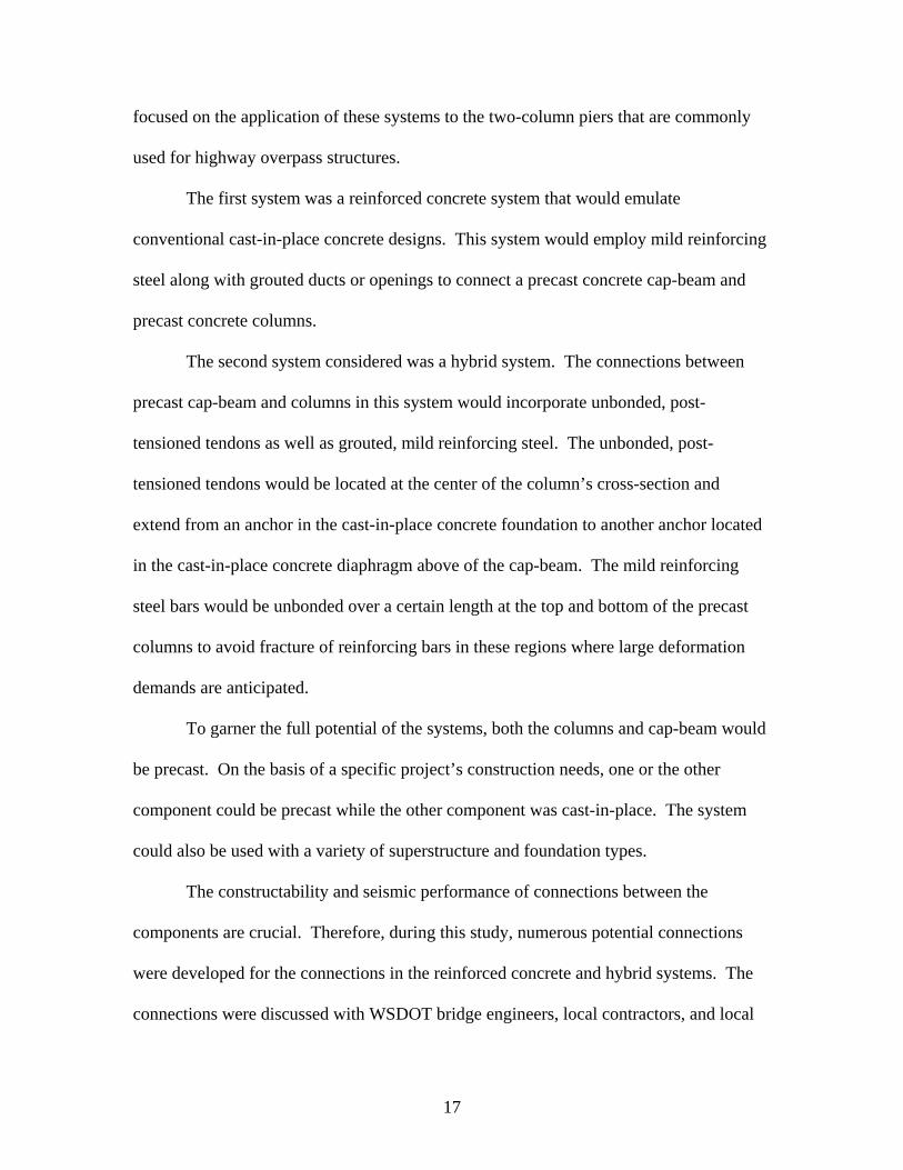
is applicable for a variety of cast-in-place concrete foundation types. Figure 3.1 shows a
sketch of a reinforced concrete pier supported on a drilled shaft foundation.
The precast concrete columns of this system emulate traditional reinforced, cast-
in-place concrete columns. The American Heritage Dictionary (2000) defines emulation
as an “effort to equal another.” Emulation of the cast-in-place column entails fabricating
a precast column on the basis of the geometry, material properties, and details of its cast-
in-place concrete counterpart. Longitudinal reinforcing steel extends from the top and
bottom of the precast column, as shown in Figure 3.1. The reinforcing steel extensions
are meant to facilitate the connection between the column and the other components. The
18
steel extending from the tops of the columns extends into ducts or openings in the precast
concrete cap-beam. A portion of the reinforcement extends through the ducts into the
cast-in-place diaphragm, while the remainder is anchored in the ducts. Bars are added
where necessary to provide the required embedment to resist the forces that develop
during a seismic event.
Figure 3.1: Elevation of Reinforced Concrete System Pier
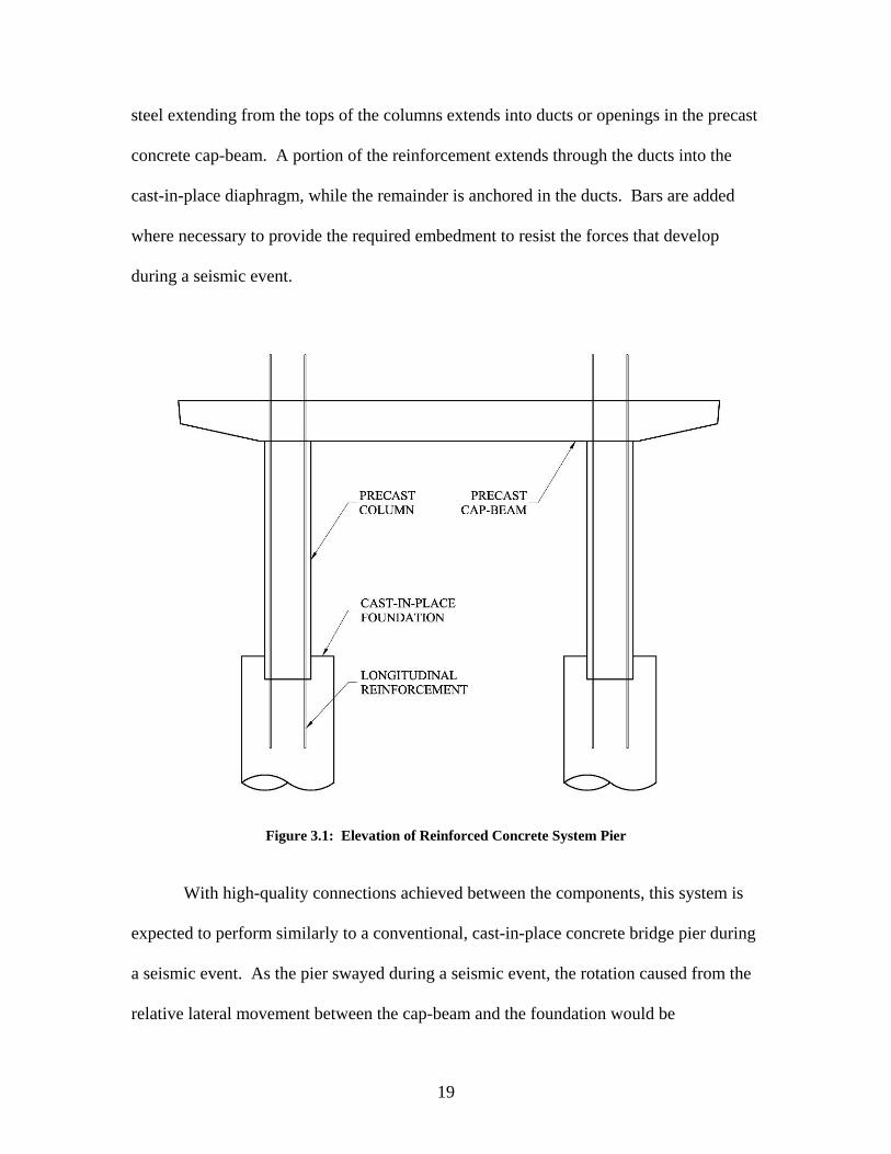
With high-quality connections achieved between the components, this system is
expected to perform similarly to a conventional, cast-in-place concrete bridge pier during
a seismic event. As the pier swayed during a seismic event, the rotation caused from the
relative lateral movement between the cap-beam and the foundation would be
19
accommodated through the development of small cracks distributed throughout plastic-
hinge regions located at the top and bottom of the columns. Figure 3.2 shows a sketch of
cracks located near the base of a column. During cyclic loading, the frame would mainly
dissipate energy through the hysteretic behavior of the mild reinforcing steel.
Figure 3.2: Expected Behavior of Connection in Reinforced Concrete Frames
3.1.2 Proposed Construction Sequence
The construction sequence for a bridge pier made with precast concrete
components would be different than that for a cast-in-place bridge pier. A proposed
construction sequence for the cast-in-place emulation system is illustrated in Figure 3.3
and is further described in this section.
20
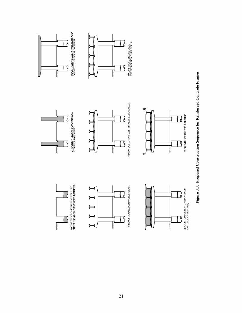
Figu
re 3
.3:
Prop
osed
Con
stru
ctio
n Se
quen
ce fo
r R
einf
orce
d C
oncr
ete
Fram
es
21
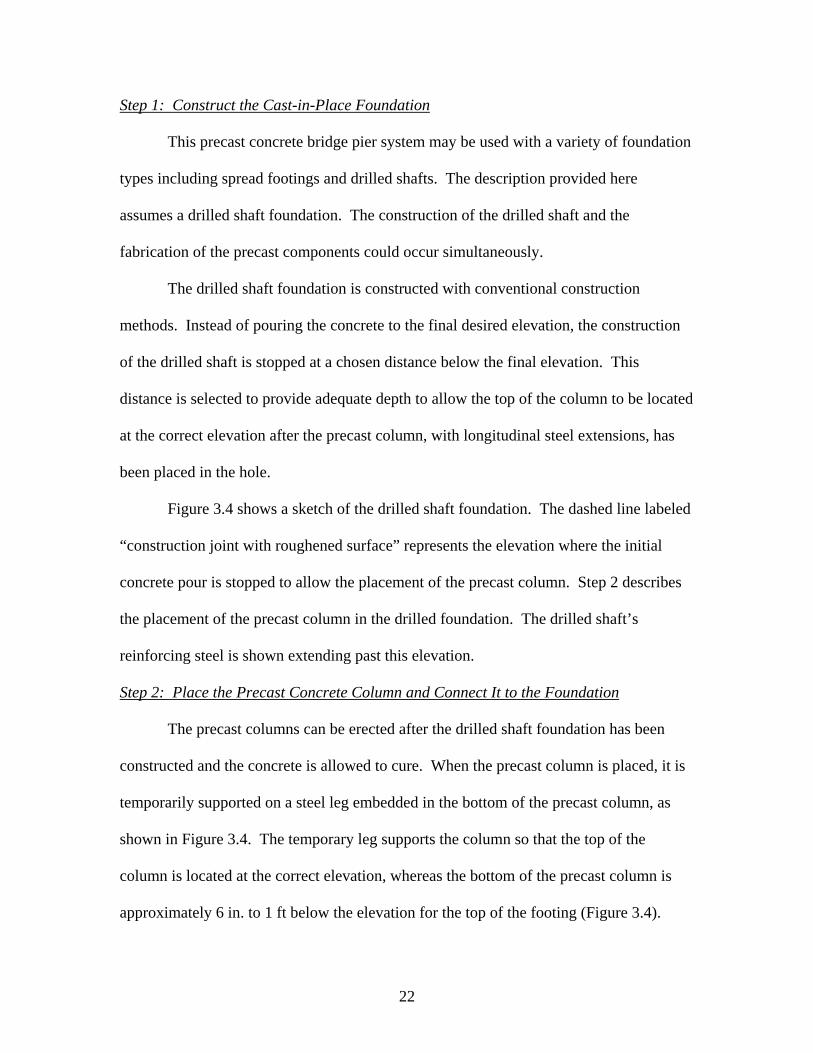
Step 1: Construct the Cast-in-Place Foundation
This precast concrete bridge pier system may be used with a variety of foundation
types including spread footings and drilled shafts. The description provided here
assumes a drilled shaft foundation. The construction of the drilled shaft and the
fabrication of the precast components could occur simultaneously.
The drilled shaft foundation is constructed with conventional construction
methods. Instead of pouring the concrete to the final desired elevation, the construction
of the drilled shaft is stopped at a chosen distance below the final elevation. This
distance is selected to provide adequate depth to allow the top of the column to be located
at the correct elevation after the precast column, with longitudinal steel extensions, has
been placed in the hole.
Figure 3.4 shows a sketch of the drilled shaft foundation. The dashed line labeled
“construction joint with roughened surface” represents the elevation where the initial
concrete pour is stopped to allow the placement of the precast column. Step 2 describes
the placement of the precast column in the drilled foundation. The drilled shaft’s
reinforcing steel is shown extending past this elevation.
Step 2: Place the Precast Concrete Column and Connect It to the Foundation
The precast columns can be erected after the drilled shaft foundation has been
constructed and the concrete is allowed to cure. When the precast column is placed, it is
temporarily supported on a steel leg embedded in the bottom of the precast column, as
shown in Figure 3.4. The temporary leg supports the column so that the top of the
column is located at the correct elevation, whereas the bottom of the precast column is
approximately 6 in. to 1 ft below the elevation for the top of the footing (Figure 3.4).
22
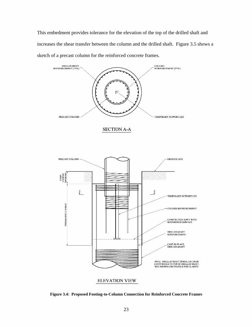
This embedment provides tolerance for the elevation of the top of the drilled shaft and
increases the shear transfer between the column and the drilled shaft. Figure 3.5 shows a
sketch of a precast column for the reinforced concrete frames.
Figure 3.4: Proposed Footing-to-Column Connection for Reinforced Concrete Frames
23
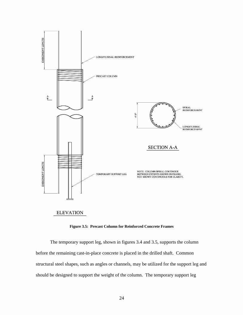
Figure 3.5: Precast Column for Reinforced Concrete Frames
The temporary support leg, shown in figures 3.4 and 3.5, supports the column
before the remaining cast-in-place concrete is placed in the drilled shaft. Common
structural steel shapes, such as angles or channels, may be utilized for the support leg and
should be designed to support the weight of the column. The temporary support leg
24
protects the column’s longitudinal reinforcing steel extensions against carrying any
gravity load during construction.
The support leg can be outfitted with a leveling mechanism, such as a series of
leveling bolts, to account for any variation in the top of the construction joint in the
drilled shaft. Otherwise, shims may be placed in the drilled shaft to adjust the column to
the required elevation. The temporary support leg supports the column in the vertical
direction, but bracing is needed to make certain that the column’s horizontal location is
correct, as well as to ensure that the column is not tilted.
After the precast column has been placed and adequately supported, the remaining
portion of the drilled shaft may be poured and allowed to cure. This completes the
connection between the foundation and the precast column. Confinement in this region is
provided by the drilled shaft’s spiral reinforcement. Placement of the concrete in this
region may become difficult because of the congestion caused by the column’s and
drilled shaft’s reinforcing steel and the lack of accessibility for the vibration of the
concrete. This is especially true for the area directly below the column. Self
consolidating concrete may be used in this region to help alleviate the problem. To
reduce the potential for air pockets developing below the column, the column base can be
tapered.
Step 3: Place the Precast Concrete Cap-Beam and Connect It to the Columns
After the precast columns are securely in place, the precast concrete cap-beam can
be placed onto the columns. The precast cap-beams described in this document are
commonly referred to as partially raised cap beams. They make use of a precast portion,
typically 3.5 ft deep, to support the girders and the deck slab during construction. A cast-
25
in-place diaphragm is then placed on top of the precast portion to create the full depth of
the cap-beam.
The connections between the column and cap-beam are critical for
constructability and good seismic performance. Two connections are proposed in Section
3.1.3. One makes use of slotted openings in the cap-beam, whereas the other makes use
of a large opening in the cap-beam. A temporary collar is used during construction to
position the cap-beam and provide support until the connection is grouted. The ease of
placement of the cap-beam onto the columns can be directly affected by the tolerance
provided in the ducts or openings in the cap-beam and the alignment of the columns. For
multi-column piers, each column has to be positioned and aligned properly in relation to
the other columns to ensure that the cap-beam will fit onto the columns. Templates can
be used to ensure that the columns are positioned and oriented properly so the cap-beam
will fit easily.
The precast portion of the cap-beam and the connections between the columns
and the cap-beam should be designed to support the weight of the girders and the fresh
deck slab concrete.
Step 4: Place the Girders on the Cap-Beam
After the precast concrete columns and cap-beam have been installed, the
sequence follows the same steps that are commonly used with cast-in-place bridge piers
and shown in WSDOT bridge standard drawings (WSDOT 2002c). The girders are
placed on the cap-beam and secured in place. Care should be taken to ensure that the
reinforcing bar extension from the column do not hinder the placement of the girders.
26
Step 5: Pour the Bottom Portion of the Cast-in-Place Diaphragm
The bottom 1-ft depth of the cast-in-place diaphragm is placed to provide lateral
and longitudinal support for the bottom of the girders, so that they do not slide from their
bearing location.
Step 6: Pour the Bridge Deck Slab Except for Portions over the Pier
The deck slab concrete is placed except for locations directly above the piers.
This allows the girders to creep, shrink, and deflect as a result of the prestressing in the
girders and the dead load from the girders and deck slab without cracking or damaging
the diaphragm.
Step 7: Pour the Top Portion of the Cast-in-Place Diaphragm and the Remaining Deck Slab
The final diaphragm pour completes the connection of the girders to the pier,
creating a deep cap-beam to resist live loads. This pour also makes the bridge continuous
for live loads because it encapsulates the mild reinforcing bars and prestressing strand
extending from the precast girder ends.
Step 8: Construct Traffic Barriers
The traffic barriers are the last components to be cast, completing the bridge
construction sequence.
General Construction Issues
Depending on the geometry of the precast component, the weight may become
excessive. Suggested weight limits for transportation and erection of the components
range up to 180,000 lbs (WSDOT 2004). These suggested weight limits permit the use of
a 48-in.-diameter column 90 ft long or a 3.5-ft by 5-ft cap-beam 65 ft long. Typical
highway overpass piers constructed in Washington State fall within these limits.
27
3.1.3 Column-to-Cap-Beam Connections
This section describes two potential column-to-cap-beam connections for the
reinforced concrete frames. Two significant difficulties that need to be overcome at the
column-to-cap-beam connection are congestion of reinforcing steel and the short
available embedment length. Embedment is needed to ensure adequate bond between the
column longitudinal reinforcing steel extensions. The first connection discussed is
called the slotted opening connection, and the second connection is called the complete
opening connection.
Slotted Opening Connection
The cap-beam is fabricated with three slots located above the column locations, as
shown in Figure 3.6. The longitudinal reinforcing bars extending from the top of the
precast column are grouped, or bundled, to allow them to fit through the slots in the cap-
beam when it is placed. Shims or a thin layer of grout may be used to level the cap-beam
on top of the column and to ensure uniform bearing. The slots are then grouted and
allowed to cure, completing the connection between the columns and the cap-beam. Use
of the slotted opening connection can provide a horizontal tolerance of approximately 3
in. in all directions.
Figure 3.6 shows sketches of the cap-beam for the slotted opening connection.
Figure 3.7 shows sketches of the cap-beam in place on top of the precast concrete
column. In Figure 3.7 the grouping of the bars is apparent.
28
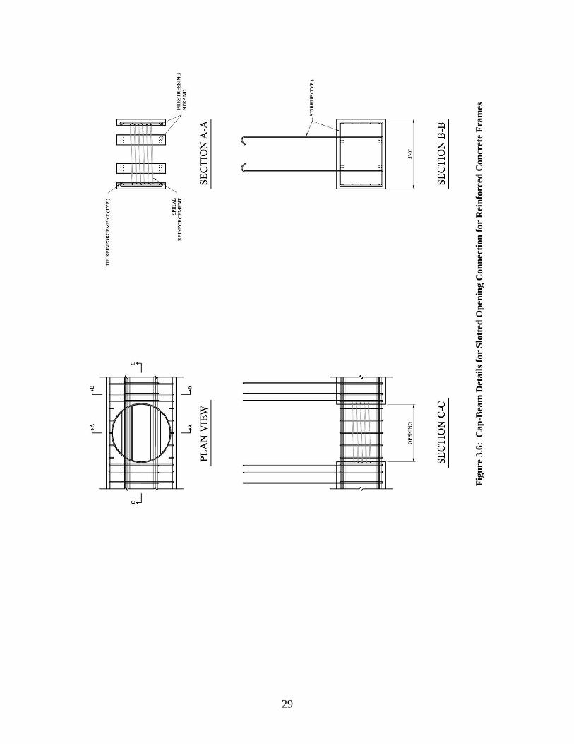
Figu
re 3
.6:
Cap
-Bea
m D
etai
ls fo
r Sl
otte
d O
peni
ng C
onne
ctio
n fo
r R
einf
orce
d C
oncr
ete
Fram
es
29
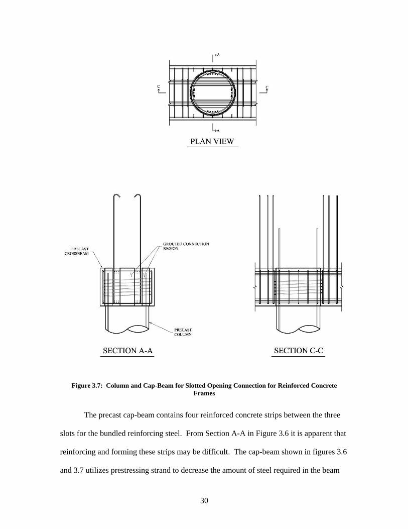
Figure 3.7: Column and Cap-Beam for Slotted Opening Connection for Reinforced Concrete Frames
The precast cap-beam contains four reinforced concrete strips between the three
slots for the bundled reinforcing steel. From Section A-A in Figure 3.6 it is apparent that
reinforcing and forming these strips may be difficult. The cap-beam shown in figures 3.6
and 3.7 utilizes prestressing strand to decrease the amount of steel required in the beam
30
for flexural resistance. Reducing the required area of steel in the cap-beam helps to
reduce the congestion in the concrete strips. If prestressing is used, the compressive
stress in the cap-beam over the column should be checked.
The concrete strips in the cap-beam above the columns must be designed for the
high moments and shear forces encountered in these areas during transportation and
erection. To increase the bearing strength of the cap-beam on the top of the columns, the
slots may be tapered (thinner opening on the top) to reduce the potential for the grout in
the slots to pop out.
Fabricating these stripped openings may present some difficulties. Although no
reinforcing penetrates the opening, the openings are thin, deep, and irregularly shaped, as
shown in Figure 3.7.
Grouping the column longitudinal bars, as shown in the plan view of Figure 3.7,
may cause some potential problems. Grouping the bars in this fashion may significantly
increase the required development lengths of the longitudinal bars in the cap-beam. This
increased development length is problematic because the available development length in
the cap-beam is limited by the depth of the cap-beam. Grouping of the bars may also
require that additional longitudinal reinforcing steel be distributed in the column to
comply with maximum spacing limits between longitudinal column bars. Grouping bars
at the column-to-cap-beam connections may also decrease the efficiency of the columns
at the critical location where plastic hinging occurs.
Complete Opening Connection
This connection is similar to the slotted opening connection except that instead of
three slotted openings the cap-beam is fabricated with one large opening located above
31
the column locations. The longitudinal reinforcing steel extending from the top of the
column passes through the large opening. During construction the cap-beam is supported
on a temporary collar located at the top of the column. The large opening is then grouted
and allowed to cure, completing the connection. Figure 3.8 shows sketches of the cap-
beam for the complete opening connection. Figure 3.9 shows sketches of the cap-beam
in place on the precast concrete column.
This connection provides tolerances similar to those found in the slotted
connection. The reinforcing bars are also distributed throughout the column’s cross-
section and the connection, which decreases the potential for pullout and provides better
load distribution in the connection.
The very thin strips of concrete on both sides of the large opening in the cap-beam
provide limited strength to resist bending and shear during transportation and erection.
Therefore, these strips need to be designed to account for these loads, possibly
incorporating prestressing steel. The large opening also introduces the potential, for the
column to punch through the cap-beam. To help alleviate this potential the opening can
be tapered.
It may be difficult to fabricate the large circular opening because the cap-beam’s
longitudinal reinforcing steel passes through the opening.
32
Figu
re 3
.8:
Cap
-Bea
m D
etai
ls fo
r C
ompl
ete
Ope
ning
Con
nect
ion
for
Rei
nfor
ced
Con
cret
e Fr
ames
33
Figure 3.9: Column and Cap-Beam for Complete Opening Connection for Reinforced Concrete Frames
3.2 HYBRID SYSTEM
This section provides a brief description of the hybrid system, a proposed
construction sequence, and details relating to the column-to-cap-beam connection.
34
3.2.1 System Description
The connections between the precast concrete columns and cap-beam in a hybrid
system are achieved with mild steel deformed bars grouted or cast into ducts or openings,
as well as unbonded prestressing strand. Because the connection uses both mild
reinforcing steel and unbonded prestressing strand, less mild reinforcing steel is required
to develop the connection than in a reinforced concrete frame. The prestressing strand is
anchored into the foundation, threaded through a duct located in the center of the column,
and anchored in the cast-in-place diaphragm. The system is applicable for a variety of
cast-in-place concrete foundation types. Figure 3.10 shows a sketch of a hybrid pier
supported on a drilled shaft foundation.
Figure 3.10: Elevation of Hybrid System Pier
35
The mild steel reinforcing bars in the columns are connected to the foundation
and cap-beam, as shown in Figure 3.10, in a manner similar to that for the reinforced
concrete frames. The prestressing tendons extend from the anchor in the foundation to an
anchor located in the cast-in-place portion of the diaphragm, as shown in Figure 3.10.
The precast columns of this system are designed so that, as the pier sways during
a seismic event, the rotation caused from the relative lateral movement between the cap-
beam and the foundation is accommodated through one gap opening at the interfaces near
the top and bottom of the column. Figure 3.11 shows a sketch of the single gap located at
the base of the column. During cyclic loading, the frame dissipates energy through the
hysteretic behavior of the mild reinforcing steel. The unbonded post-tensioning tendons
are designed so that they do not yield. By remaining elastic, the tendons do not provide
any energy dissipation, but they do provide re-centering ability. The re-centering ability
causes hybrid piers to have small residual displacements after an earthquake. The
unbonded post-tensioning does not yield because the increase in strain as the frame sways
is distributed over the length of the entire tendon. The deformed bars are anchored in the
adjacent components with grouted sleeves, which provide much higher bond capacity
than embedment in concrete. To prevent bar fracturing caused by large strain
concentrations at the gap, it is necessary to debond the bars for a short distance on either
side of the interface.
This system allows the proportion of mild reinforcing steel and unbonded
prestressing tendon to be selected on the basis of the required response, either providing
an increased re-centering ability or additional energy dissipation to limit maximum
displacements.
36
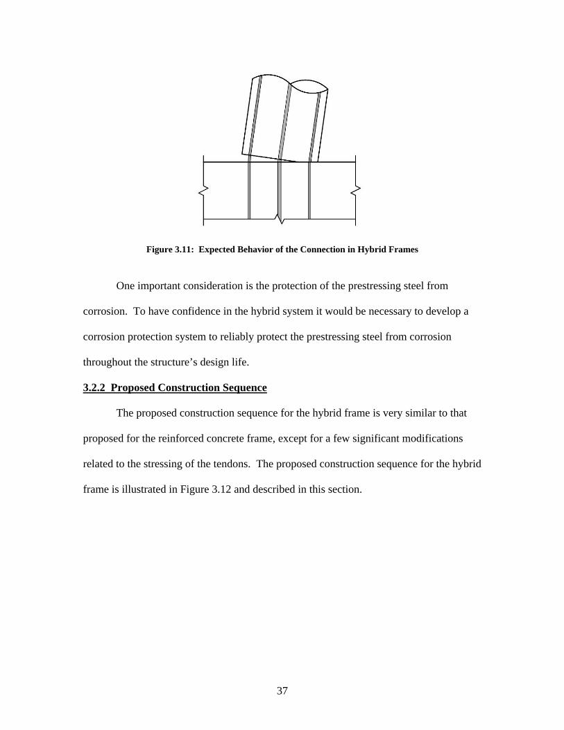
Figure 3.11: Expected Behavior of the Connection in Hybrid Frames
One important consideration is the protection of the prestressing steel from
corrosion. To have confidence in the hybrid system it would be necessary to develop a
corrosion protection system to reliably protect the prestressing steel from corrosion
throughout the structure’s design life.
3.2.2 Proposed Construction Sequence
The proposed construction sequence for the hybrid frame is very similar to that
proposed for the reinforced concrete frame, except for a few significant modifications
related to the stressing of the tendons. The proposed construction sequence for the hybrid
frame is illustrated in Figure 3.12 and described in this section.
37
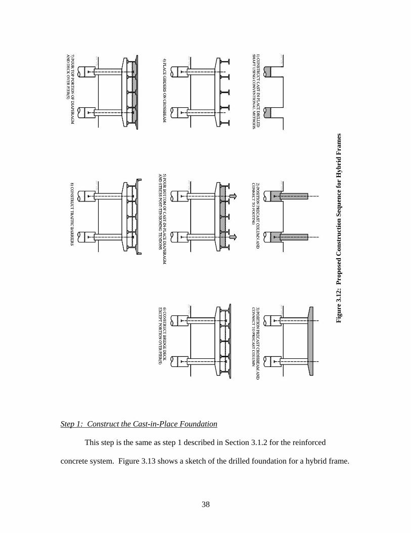
Figu
re 3
.12:
Pro
pose
d C
onst
ruct
ion
Sequ
ence
for
Hyb
rid
Fram
es
Step 1: Construct the Cast-in-Place Foundation
This step is the same as step 1 described in Section 3.1.2 for the reinforced
concrete system. Figure 3.13 shows a sketch of the drilled foundation for a hybrid frame.
38
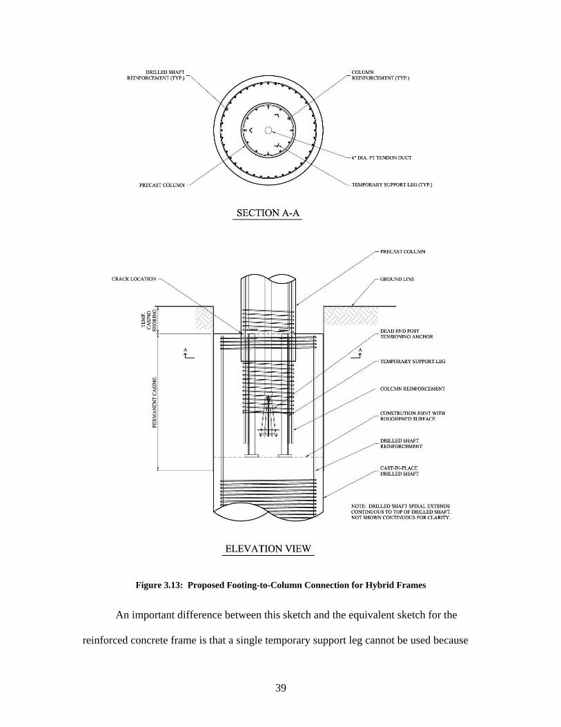
Figure 3.13: Proposed Footing-to-Column Connection for Hybrid Frames
An important difference between this sketch and the equivalent sketch for the
reinforced concrete frame is that a single temporary support leg cannot be used because
39
the prestressing anchor is located directly below the center of the column. Instead, three
small temporary support legs are used, allowing the post-tensioning tendons to extend out
from the center of the column to the prestressing anchor in the foundation. Another
important difference is the dashed line labeled “crack location” in Figure 3.13. The
column is designed to crack, or develop a gap, as shown in Figure 3.11, at this location.
This crack location will be described further in Section 3.2.3.
Step 2: Place the Precast Concrete Column and Connect It to the Foundation
This step is similar to step 2 for the reinforced concrete frame. Figure 3.14 shows
a sketch of a column for a hybrid frame. The key differences are the inclusion of the
post-tensioning strand and the designated cracking location.
The temporary support legs, shown in figures 3.13 and 3.14, allow the column to
be supported at the correct elevation before the remaining cast-in-place concrete is placed
in the drilled shaft. They also create a space to place the prestressing anchor. The length
of the longitudinal extensions is based on the necessary bond length required to transfer
the force between the drilled shaft and the column. The prestressing anchor should be
located far enough below the bottom of the column to ensure that the prestressing force
has transferred to the concrete by the time it reaches the base of the column.
40
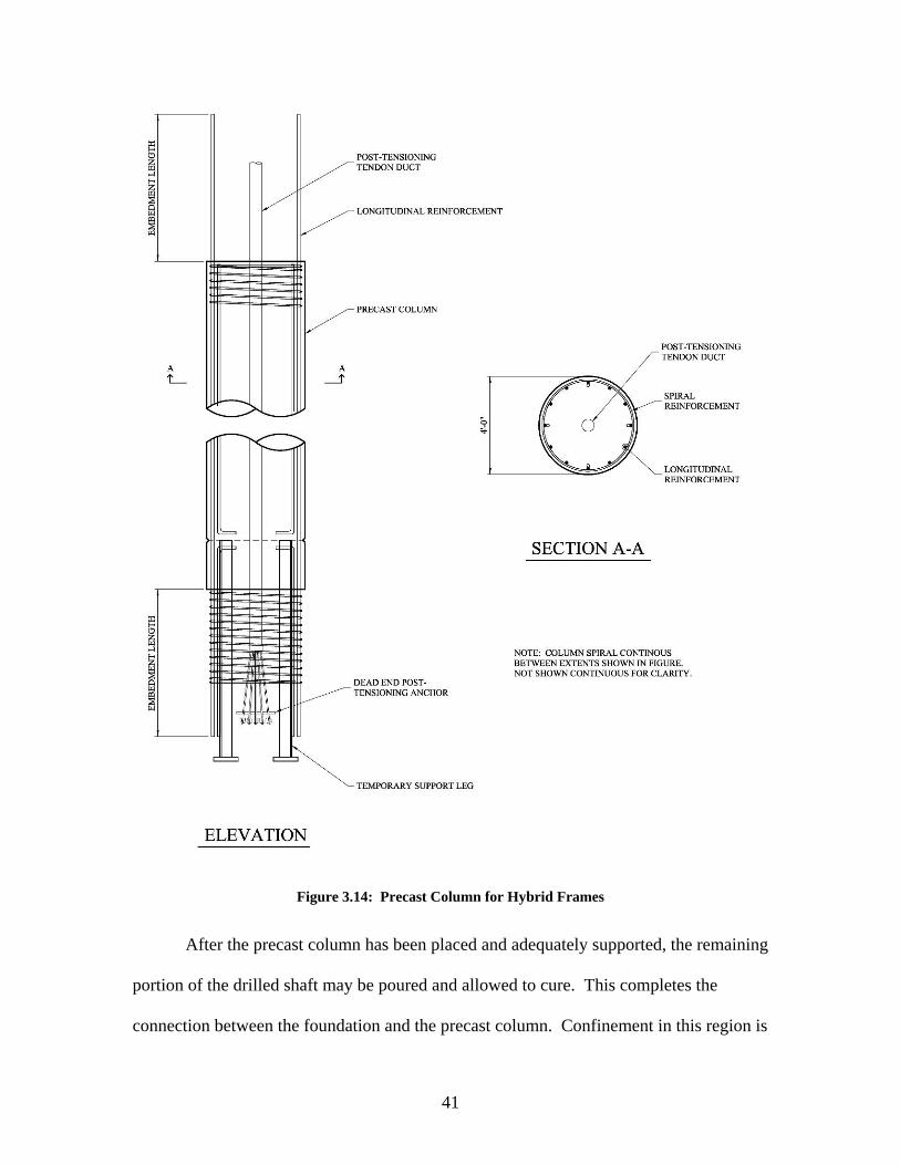
Figure 3.14: Precast Column for Hybrid Frames
After the precast column has been placed and adequately supported, the remaining
portion of the drilled shaft may be poured and allowed to cure. This completes the
connection between the foundation and the precast column. Confinement in this region is
41
provided by the drilled shaft’s spiral reinforcement. Placement of the concrete in this
region may become difficult because of the congestion caused by the column’s and
drilled shaft’s reinforcement steel, the lack of accessibility for the vibration of the
concrete, and the prestressing anchor. This is especially true for the area directly below
the column. Self consolidating concrete may be used in this region to help alleviate the
problem. To reduce the potential for air pockets developing below the column, the
column base may be tapered.
Step 3: Place the Precast Concrete Cap-Beam and Connect It to the Columns
This step is similar to step 3 for the reinforced concrete frame. The important
difference is the need to thread the post-tensioning strand through the ducts or opening in
the cap beam and secure it until the anchor is placed in the cast-in-place diaphragm.
The connections between the column and cap-beam are critical for
constructability and good seismic performance. The two connections described in
Section 3.1.3 can be modified for use with the hybrid system. Essentially, the only
changes required are to include the prestressing strand and to reduce the number of mild
reinforcing steel bars. Reducing the number of required reinforcing bars can significantly
help reduce the congestion in this connection. Section 3.2.3 describes one other
connection, which employs individual splice sleeves, that may be used for the hybrid
system.
Step 4: Place the Girders on the Cap-Beam
This step is the same as step 4 for the reinforced concrete system.
42
Step 5: Pour the Bottom Portion of the Cast-in-Place Diaphragm and the Stress Post-Tensioning Tendons
This step is the same as step 5 for the reinforced concrete system except that the
depth of the pour may have to be increased to accommodate the placement of the
prestressing anchors in the cast-in-place diaphragm.
After the prestressing anchors have been placed and the concrete in the diaphragm
has been allowed to cure, the prestressing tendons are stressed, completing the connection
between the cap-beam and the column.
Step 6: Pour the Bridge Deck Slab Except for Portions over the Pier
This step is the same as step 6 for the reinforced concrete system.
Step 7: Pour the Top Portion of the Cast-in-Place Diaphragm and the Remaining Deck Slab
This step is the same as step 7 for the reinforced concrete system.
Step 8: Construct Traffic Barriers
The traffic barriers are the last components to be cast.
General Construction Issues
Care must be taken to ensure that the prestressing steel and the anchorages are not
exposed to agents that could cause corrosion. An acceptable corrosion prevention system
must be developed to ensure complete protection of the strand and anchors throughout
the life of the structure.
3.2.3 Details of Column-to-Cap-Beam Connections
The connections described in Section 3.1.3 could also be used for the hybrid
system with slight modifications, such as the inclusion of post-tensioning strand and
anchors. The number of mild reinforcing bars could also be reduced. This section
describes a third connection that can be used for the hybrid system. Because the hybrid
43
frame requires less mild reinforcing steel, individual splice sleeves can be used to connect
the cap-beam to the columns. As the cap-beam is lowered onto the columns, each
individual splice sleeve receives a mild reinforcing bar. Use of individual splice sleeves
makes fabrication easier because the sleeves do not need to be removed after fabrication.
Grouting of the individual splice sleeves may be difficult because of the limited
clearance between the sides of the splice sleeves and the reinforcing bar. Also the limited
tolerance provided by the splice sleeve may make the placement of the cap-beam on the
column difficult. Figures 3.15 and 3.16 show the details for the individual splice sleeve
connection.
44
Figu
re 3
.15:
Cap
-Bea
m D
etai
ls fo
r In
divi
dual
Spl
ice
Slee
ve C
onne
ctio
n fo
r H
ybri
d Fr
ames
45
Figure 3.16: Column and Cap-Beam for Individual Splice Sleeve Connection for Hybrid Frames
46
CHAPTER 4 ANALYTICAL MODEL
Analytical models of the proposed bridge systems presented in Chapter 3 were
developed to establish the systems’ key characteristics, as well as to investigate their
global responses to seismic loading.
A two-dimensional, nonlinear finite element model of a single frame was used to
model the response of the proposed pier systems. The analyses included monotonic
pushover analyses and dynamic earthquake analyses. An object-oriented framework used
for nonlinear finite-element analyses, Open Systems for Earthquake Engineering
Simulation (OpenSees), was used to create the models and perform the analyses
(OpenSees 2000; Fenves et al. 2004). One of the important benefits of OpenSees is that
it uses the scripting language Tcl to enter the commands for modeling frame geometry,
applying static and dynamic loading, and defining solution formulations. The scripting
language facilitates the execution of parametric studies by allowing analyses of various
system configurations through repetitive looping of the analysis script. OpenSees was
also selected for this study because, in recent years, OpenSees has seen increasing use,
especially in the research community, and accommodates parametric studies. The Tcl
script written during this research, which was generated to create the nonlinear finite-
element models of the proposed bridge systems and perform the analyses, was described
by Hieber (2005).
This chapter describes the prototype bridge that was selected for this study
(Section 4.1), followed by the baseline characteristics for the proposed bridge systems
described in Chapter 3 (Section 4.2), column characteristics (Section 4.3), cap-beam
47
characteristics (Section 4.4), and joint characteristics (Section 4.5). The methodologies
used for the pushover analyses (Section 4.6) and the earthquake analyses (Section 4.7)
are then described.
4.1 PROTOTYPE BRIDGE
A prototype bridge was selected to guide the development of the numerical
models in OpenSees. The prototype bridge established the geometric conditions, design
details, and material properties of the baseline frames for the proposed bridge systems.
The following points were considered in selecting the prototype bridge from plans
provided by WSDOT.
• Located in western Washington State
• Typical highway bridge configuration
• Designed with details similar to those currently used by WSDOT
The prototype bridge selected for this study was the three-span, prestressed
concrete girder structure carrying State Route 18 over State Route 516 in King County,
Washington (WSDOT 1996). The bridge was designed in 1995 on the basis of
requirements found in the 1994 AASHTO LRFD Bridge Design Specifications and the
AASHTO Standard Specifications for Highway Bridges, Fifteenth Edition.
The bridge is 297 ft long with spans of 80 ft, 137 ft, and 80 ft located on a tangent
horizontal alignment. The superstructure is 38 ft wide and consists of five 74-in.-deep,
Washington standard prestressed concrete girders (W74G) with a composite, reinforced
concrete deck, 7.5-in. thick, supported on laminated elastomeric bearing pads. The
bridge is continuous for live load.
48
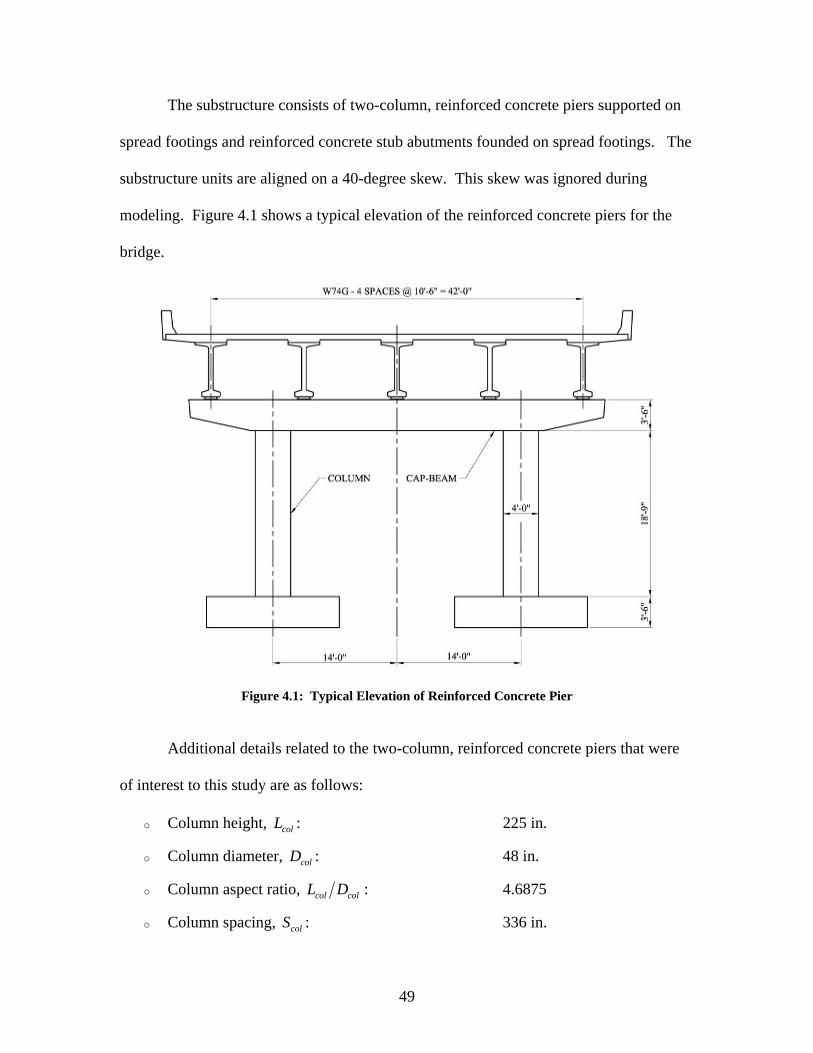
The substructure consists of two-column, reinforced concrete piers supported on
spread footings and reinforced concrete stub abutments founded on spread footings. The
substructure units are aligned on a 40-degree skew. This skew was ignored during
modeling. Figure 4.1 shows a typical elevation of the reinforced concrete piers for the
bridge.
Figure 4.1: Typical Elevation of Reinforced Concrete Pier
Additional details related to the two-column, reinforced concrete piers that were
of interest to this study are as follows:
o Column height, : 225 in. colL
o Column diameter, : 48 in. colD
o Column aspect ratio, col colL D : 4.6875
o Column spacing, : 336 in. colS
49
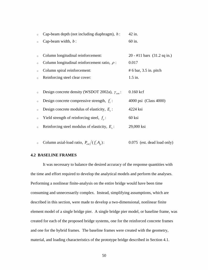
o Cap-beam depth (not including diaphragm), : 42 in. h
o Cap-beam width, : 60 in. b
o Column longitudinal reinforcement: 20 - #11 bars (31.2 sq in.)
o Column longitudinal reinforcement ratio, ρ : 0.017
o Column spiral reinforcement: # 6 bar, 3.5 in. pitch
o Reinforcing steel clear cover: 1.5 in.
o Design concrete density (WSDOT 2002a), conγ : 0.160 kcf
o Design concrete compressive strength, 'cf : 4000 psi (Class 4000)
o Design concrete modulus of elasticity, : 4224 ksi cE
o Yield strength of reinforcing steel, yf : 60 ksi
o Reinforcing steel modulus of elasticity, sE : 29,000 ksi
o Column axial-load ratio, '( )col c gP f A : 0.075 (est. dead load only)
4.2 BASELINE FRAMES
It was necessary to balance the desired accuracy of the response quantities with
the time and effort required to develop the analytical models and perform the analyses.
Performing a nonlinear finite-analysis on the entire bridge would have been time
consuming and unnecessarily complex. Instead, simplifying assumptions, which are
described in this section, were made to develop a two-dimensional, nonlinear finite
element model of a single bridge pier. A single bridge pier model, or baseline frame, was
created for each of the proposed bridge systems, one for the reinforced concrete frames
and one for the hybrid frames. The baseline frames were created with the geometry,
material, and loading characteristics of the prototype bridge described in Section 4.1.
50
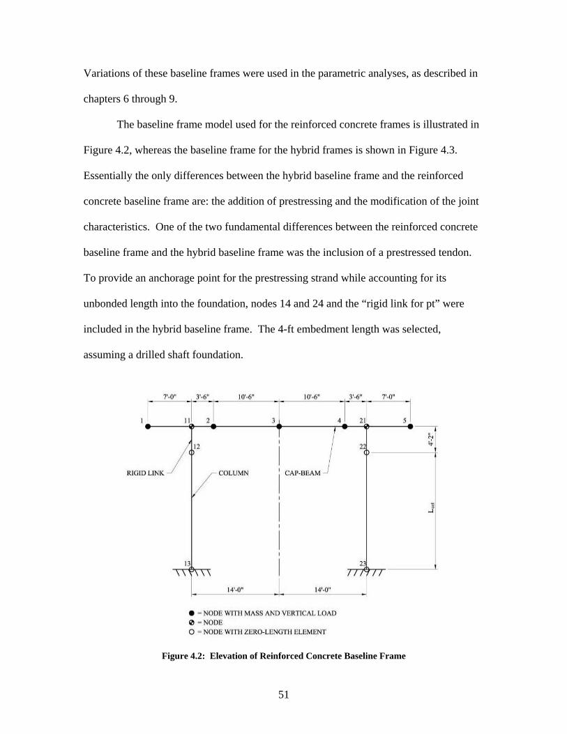
Variations of these baseline frames were used in the parametric analyses, as described in
chapters 6 through 9.
The baseline frame model used for the reinforced concrete frames is illustrated in
Figure 4.2, whereas the baseline frame for the hybrid frames is shown in Figure 4.3.
Essentially the only differences between the hybrid baseline frame and the reinforced
concrete baseline frame are: the addition of prestressing and the modification of the joint
characteristics. One of the two fundamental differences between the reinforced concrete
baseline frame and the hybrid baseline frame was the inclusion of a prestressed tendon.
To provide an anchorage point for the prestressing strand while accounting for its
unbonded length into the foundation, nodes 14 and 24 and the “rigid link for pt” were
included in the hybrid baseline frame. The 4-ft embedment length was selected,
assuming a drilled shaft foundation.
Figure 4.2: Elevation of Reinforced Concrete Baseline Frame
51
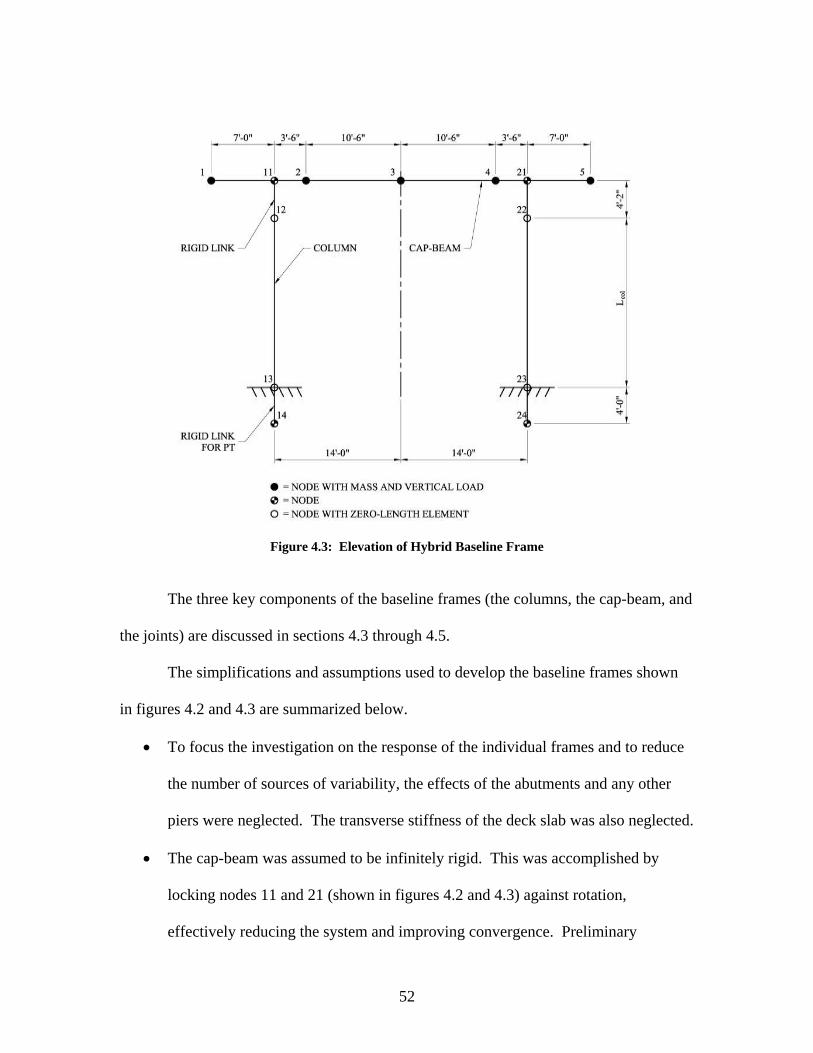
Figure 4.3: Elevation of Hybrid Baseline Frame
The three key components of the baseline frames (the columns, the cap-beam, and
the joints) are discussed in sections 4.3 through 4.5.
The simplifications and assumptions used to develop the baseline frames shown
in figures 4.2 and 4.3 are summarized below.
• To focus the investigation on the response of the individual frames and to reduce
the number of sources of variability, the effects of the abutments and any other
piers were neglected. The transverse stiffness of the deck slab was also neglected.
• The cap-beam was assumed to be infinitely rigid. This was accomplished by
locking nodes 11 and 21 (shown in figures 4.2 and 4.3) against rotation,
effectively reducing the system and improving convergence. Preliminary
52
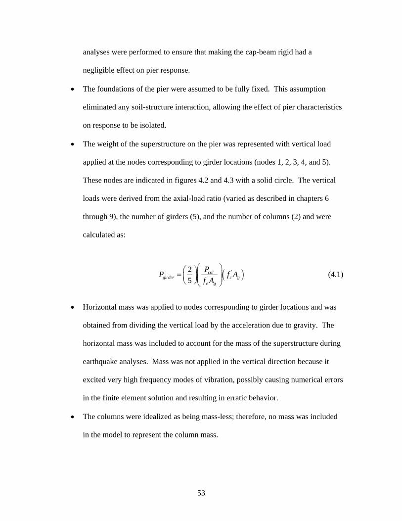
analyses were performed to ensure that making the cap-beam rigid had a
negligible effect on pier response.
• The foundations of the pier were assumed to be fully fixed. This assumption
eliminated any soil-structure interaction, allowing the effect of pier characteristics
on response to be isolated.
• The weight of the superstructure on the pier was represented with vertical load
applied at the nodes corresponding to girder locations (nodes 1, 2, 3, 4, and 5).
These nodes are indicated in figures 4.2 and 4.3 with a solid circle. The vertical
loads were derived from the axial-load ratio (varied as described in chapters 6
through 9), the number of girders (5), and the number of columns (2) and were
calculated as:
( ''
25
col )girder c gc g
PPf A
⎛ ⎞⎛ ⎞= ⎜ ⎟⎜ ⎟⎜ ⎟⎝ ⎠⎝ ⎠f A (4.1)
• Horizontal mass was applied to nodes corresponding to girder locations and was
obtained from dividing the vertical load by the acceleration due to gravity. The
horizontal mass was included to account for the mass of the superstructure during
earthquake analyses. Mass was not applied in the vertical direction because it
excited very high frequency modes of vibration, possibly causing numerical errors
in the finite element solution and resulting in erratic behavior.
• The columns were idealized as being mass-less; therefore, no mass was included
in the model to represent the column mass.
53
• No viscous damping was considered in this study because of inconsistencies in
pier response when damping was included. Priestley et al. (1996) indicated that
Coulomb (friction) damping, radiation damping, and hysteretic damping are more
common forms of damping for bridges than viscous damping. Coulomb damping
typically occurs as movement takes place in bearings, connections, and joints.
Radiation damping occurs as a consequence of soil-structure interaction and refers
to the dissipation of energy as it spreads over an increasing volume of soil
surrounding a bridge’s foundation (Kramer 1996). Hysteretic damping refers to
the energy dissipated during cyclic displacements and is found from the area
within the hysteresis loop of the force-displacement response (Chopra 2001).
Bridges have few nonstructural elements and, consequently, few obvious sources
of damping that are not accounted for by hysteresis in the structural elements or
radiation into the soil. Wacker (2005) found that the equivalent damping ratio for
the hysteretic damping alone ranged between 10 and 25 percent. Because the
damping modeled as viscous is likely much smaller than the hysteretic damping,
the impact of ignoring it is likely to be small. Coulomb damping and radiation
damping were also ignored during the analyses.
4.3 COLUMN CHARACTERISTICS
This section describes the characteristics of the columns created for the baseline
frames, including geometric characteristics, modeling characteristics, and material
characteristics.
• A constant column diameter of 48 in. was selected for the baseline frames. The
basis for this assumption is presented in Chapter 6.
54
• The length of the column, , was defined as the clear height between the top of
the foundation and the bottom of the cap-beam. This quantity was varied as
described in chapters 6 through 9.
colL
• The circular columns were modeled as force-based, nonlinearBeamColumn
elements with a fiber cross-section. The force-based elements considered the
spread of plasticity along the length of the column. They were used during this
study, instead of displacement-based elements, because they provided the ability
to model nonlinearity with a single element for each structural member (Coleman
and Spacone 2001). The fiber cross-section was defined by the column’s cross-
sectional geometry, the number of longitudinal reinforcement bars, and material
properties.
• Five integration points were used along the length of the nonlinearBeamColumn
element.
• The fiber cross-section contained three discretized sub-regions: the cover layer of
unconfined concrete, the inner core region containing confined concrete, and the
circular layer of longitudinal reinforcing steel. As part of his ongoing doctoral
research study at the University of Washington, Michael Berry performed a study
investigating the effect of the number of subdivisions chosen for the fiber cross-
section and recommended the following for this study:
o Number of subdivisions in the circumferential direction for the core: 20
o Number of subdivisions in the radial direction for the core: 10
o Number of subdivisions in the circumferential direction for the cover: 20
o Number of subdivisions in the radial direction for the cover: 5
55
These values were used during the earthquake analyses to achieve accurate results
in a reasonable time. Because the pushover analyses were less computationally
intensive, the mesh size was halved to estimate the response more accurately.
• The cross-sectional area corresponding to a #11 deformed bar was used when the
circular layer of longitudinal reinforcement steel was defined. By using the area
corresponding to the #11 deformed bar, the actual longitudinal reinforcement
ratio, ρ or eqρ , varied slightly in comparison to the target values described in
chapters 6 through 9. To ensure symmetric placement of the bars about the
column’s axis of bending, an even number of bars was used for all of the
columns.
• Material type Concrete02 was used to model the unconfined, cover concrete.
Concrete02 uses the modified Kent-Park model to represent the concrete
compressive stress-strain curve and straight lines for the rising and falling
segments of the tension region. The modified Kent-Park stress-strain curve
consists of a parabolic curve up to the concrete compressive strength followed by
a downward sloping line to the concrete crushing strength (Kent and Park 1971).
This representation is commonly used and is a modification of the one proposed
by Hognestad (1951). The unloading stress-strain characteristics are based on
Karsan and Jirsa (1969). Concrete02 was selected because it provides tension
strength and linear tension softening. The following material properties were
used to model the unconfined, cover concrete:
o Concrete compressive strength, 'cf : 5.0 ksi
o Strain at concrete compressive strength, 0cε : 0.002
56
o Ultimate concrete compressive strength, cuf : 0.0 ksi
o Strain at ultimate concrete compressive strength, cuε : 0.005
o Initial slope on stress-strain curve (OpenSees 2000), : cE '02 c cf ε
o Concrete tensile strength (MacGregor 1997), rf : '7.5 cf
o Tension softening slope, : tE cE−
Although 0.003 is a common value assumed for cuε in design (MacGregor 1997),
the value of 0.005 was selected on the basis of the minimum crushing strain in
cover concrete presented by Park et al. (1982). The expression for is derived
from the geometry of a parabola.
cE
• The confined core concrete was modeled by using a new OpenSees material
component, Concrete04, created by Nilanjan Mitra at the University of
Washington. Concrete04 is a modification of Concrete02 that uses the pre- and
post-peak curves proposed by Popovics (1973). Unlike the parabola used in the
Kent-Park model that is defined by 'cf and 0cε (the initial modulus of elasticity is
found from the geometry of the parabola), the curves proposed by Popovics
(1973) account for 'cf , 0cε , and . As suggested by Priestley et al. (1996), the
confined core concrete was modeled with no tension strength. On the basis of the
properties presented above for the unconfined concrete, the following material
properties were calculated for the confined concrete from the equations provided
by Mander et al. (1988).
cE
o Concrete compressive strength, 'cf : 7.0 ksi
o Strain at concrete compressive strength, 0cε : 0.006
o Ultimate concrete compressive strength, cuf : 5.9 ksi
57
o Strain at ultimate concrete compressive strength, cuε : 0.020
o Initial slope on stress-strain curve (WSDOT 2002(a)), : 4722 ksi cE
• The deformed mild steel reinforcement was modeled by using Steel02, which uses
the envelope from the commonly assumed bilinear stress-strain curve. To
characterize the shape of the unloading branch, the Menegotto-Pinto (1973)
equation is used to simulate the Bauschinger effect, in which nonlinear response
develops at strains significantly lower than the yield strain (Paulay and Priestley
1992). The following material properties were used to define the reinforcing
steel:
o Modulus of elasticity of mild steel, sE : 29,000 ksi
o Yield strength of mild steel, yf : 60 ksi
o Strain at yield strength of mild steel, yε : y sf E
o Ultimate strength of mild steel, uf : 90 ksi
o Strain at ultimate strength of mild steel, uε : 0.12
o Stain hardening ratio, : SHR ( ) ( )u y u y sf f Eε ε⎡ ⎤− −⎣ ⎦
• For the hybrid frames, the prestressing steel was modeled with an
elasticBeamColumn element, with a modulus of elasticity of 28,500 ksi and
negligible bending stiffness. An elasticBeamColumn element with negligible
bending stiffness was used to represent the prestressing steel because truss
elements cannot support thermal stresses in OpenSees. The prestressing was
induced by applying a thermal stress to the element, as described in Wacker et al.
(2005).
58
4.4 CAP-BEAM CHARACTERISTICS
Two components were used to represent the cap-beam. The first, shown as “Cap-
Beam” in figures 4.2 and 4.3, represented the horizontal elements of the cap-beam that
connect the nodes in the cap-beam. The elements were located at the elastic neutral axis
of the cap-beam. The second component, shown as “Rigid Link” in the figures, was
included to represent the finite size of the column-to-cap-beam joint, which was assumed
to remain rigid.
It was assumed that the cap-beam would remain elastic during the analyses;
therefore, it was modeled with an elasticBeamColumn. The cross-sectional area and the
moment of inertia of the cap-beam elements were found for the prototype bridge’s cap-
beam, both with and without consideration for the contribution of the deck slab. The
averages of these values were used for the baseline frames of this study. The resulting
cross-section area and moment of inertia were 4920 in.2 and 6,230,000 in.4, respectively.
To ensure that flexural deformations in the rigid links would be negligible in comparison
to the column deformations, they were given a cross-sectional area equal to the column’s
cross-sectional area and a moment of inertia 1000 times larger than the value used for the
cap-beam.
4.5 JOINT CHARACTERISTICS
The reinforced concrete and hybrid baseline frames differed in the characteristics
used to model the joints between the columns and the foundation and cap-beam (nodes
12, 13, 22, and 23 in figures 4.2 and 4.3). The joints were modeled using the
zeroLengthSection element in OpenSees, which defines two nodes at the same location.
59
The zero length sections were given force-deformation relationships to represent the
desired properties of the joints.
For the reinforced concrete baseline frame, the joints were given properties to
represent the Lehman Bond-Slip Model (Lehman and Moehle 2000). This model was
selected to represent the bond between the tension reinforcing steel and the concrete. The
concrete in the joint was modeled by using Concrete04 with the confined concrete
properties defined in Section 4.4. The reinforcing steel was modeled by using a
Hysteretic uniaxialMaterial in OpenSees with properties defined by the equations
provided in Lehman and Moehle (2000).
For the hybrid baseline frame, the mild longitudinal reinforcing steel is unbonded
for a given length, so the Lehman Bond Model was not used. The hybrid frames were
developed to allow a crack to open at the joints at the top and bottom of the column.
Therefore, it was necessary to develop properties for the joint that could simulate the
opening of the joint. Wacker et al. (2005) developed a means of modeling this crack
formation by modifying the reinforcing steel’s stress-strain relationship by a factor to
account for the unbonded length. The concrete’s stress-strain relationship was also
modified to account for an effective compressive depth of the foundation.
Additional information relating to the joints in the reinforced concrete and hybrid
frames maybe be found in Wacker et al. (2005). Zero length elements were used to
consider the stress-deformation relationship.
4.6 METHODOLOGY FOR PUSHOVER ANALYSES
In a displacement-controlled pushover analysis, the horizontal force applied to the
frame is increased until the control node displaces by a specified distance. For this
60
study, the control node was located at the joint between the top of the rigid link and the
cap-beam above the left column (node 11 in figures 4.2 and 4.3). Other characteristics of
the pushover analyses included the following:
• The gravity loads described in this chapter were applied to the frame before the
pushover analyses.
• For the hybrid frames, the post-tensioning force described in this chapter was
applied to the frame before the pushover analyses.
• The OpenSees displacement controlled integrator, DisplacementControl, was
used to apply the horizontal load (OpenSees 2000).
• A displacement step of 0.01 in. was used during the study.
• The frames were pushed to a maximum displacement of 24 in.
• Second-order effects were considered by using the OpenSees geometric
transformation PDelta (OpenSees 2000).
P − Δ
• A tolerance of 1.0e-6 and a maximum of 100 Newton-Raphson iterations per step
were used with OpenSees’s NormDispIncr to test force convergence (OpenSees
2000).
4.7 METHODOLOGY FOR EARTHQUAKE ANALYSES
Earthquake analyses were conducted for the 10 ground motions described in
Chapter 5, five representing an event having a peak ground acceleration with a 10 percent
probability of exceedance in 50 years and five representing an event having a peak
ground acceleration with a 2 percent probability of exceedance in 50 years. Other
characteristics of the earthquake analyses included the following:
61
• The gravity loads described in this chapter were applied to the model before the
earthquake analysis began.
• For the hybrid frames, the post-tensioning force described in this chapter was
applied to the frame before the earthquake analyses began.
• The OpenSees load pattern, UniformExcitation, was used with the implicit
Newmark integration procedure.
• A time step, , equal to tΔ , 5t motionΔ was used for the earthquake analysis,
where was the time step of the ground motion’s time history. To ensure
numerical stability, Chopra (2001) suggested employing a time step of
,t motionΔ
t nT πΔ ≤
but also noted that in most earthquake analysis a smaller tΔ , generally between
0.01 to 0.02 sec., is required to accurately define the response. To eliminate
several convergence problems, it was necessary to use a time step equal to
, 5t motionΔ during this study. This resulted in time steps between 0.001 sec. and
0.005 sec., varying on the basis of the ground motion’s original time step.
• Second-order effects were considered by using the OpenSees geometric
transformation object PDelta (OpenSees 2000).
P − Δ
• A tolerance of 1.0e-6 and a maximum of 100 Newton-Raphson iterations per step
were used with OpenSees’s NormDispIncr to test force convergence (OpenSees
2000).
62
CHAPTER 5 SELECTION OF GROUND MOTIONS
This chapter describes the development of the ground motions for the dynamic
analyses described in chapters 7 and 9.
The principal goal of this study was to develop rapid bridge construction systems
for use in Western Washington State. Therefore, the WSDOT Bridge Design Manual
(WSDOT 2002a), hereafter referred to as the BDM, was consulted for guidance on
typical practice relating to the seismic design of bridges. Article 4.1.5 of the BDM refers
readers to the American Association of State Highway and Transportation Officials
(AASHTO) Bridge Design Specifications (AASHTO 1998) and the U.S. Geological
Survey’s (USGS) ground acceleration maps for all seismic requirements.
To generate the suite of ground motions, two seismic hazard levels were selected,
one representing events having a peak ground acceleration with a 10 percent probability
of exceedance in 50 years (10 percent in 50) and one representing events having a peak
ground acceleration with a 2 percent probability of exceedance in 50 years (2 percent in
50) (Section 5.1). For both levels of hazard, a database containing motions similar to
those likely to occur in Western Washington State was selected (Section 5.2). Sixteen
two-component time histories were chosen from the database, and an acceleration
response spectrum was created for each of these ground motions (Section 5.3). The 10
percent in 50 and the 2 percent in 50 design acceleration response spectra were created as
target spectra for the scaling procedure (Section 5.4). Each acceleration response
spectrum was scaled to minimize the squared error between the acceleration response
spectrum and the design acceleration response spectrum (Section 5.5). Finally, ten
63
ground motions were chosen from the scaled database for inclusion in the ground motion
suite (Section 5.6).
5.1 SELECTION OF SEISMIC HAZARD LEVEL
To evaluate the seismic hazard at a given location, possible sources of seismic
activity that could affect the location are identified and their potential for future seismic
activity is determined. This process of evaluating the seismic hazard for a given location
is referred to as a seismic hazard analysis. A seismic hazard analysis involves
investigating the geologic evidence, applicable fault activity, magnitude indicators (such
as potential fault rupture length or fault rupture area), tectonic evidence, historic
seismicity, and instrumental seismicity to estimate the seismic hazard for the given
location (Kramer 1996).
Because the proposed bridge systems were developed for use in Western
Washington State rather than a particular location, a site-specific seismic hazard analysis
was not performed. Instead, a suite of spectrum-compatible ground motions similar to
those that could occur in Western Washington State was developed for two target levels
of hazard.
The AASHTO specifications are based on a design-level earthquake with a
uniform risk model of seismic hazard with a 10 percent probability of exceedance in a
50-year period (corresponding to a return period approximately equal to 475 years), as
discussed in AASHTO Article C.3.10.2. To examine the global response of the proposed
bridge systems to design-level earthquakes, ground motions were selected and developed
that represented events with a 10 percent probability of exceedance in 50 years (10
percent in 50).
64
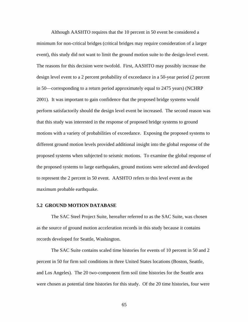
Although AASHTO requires that the 10 percent in 50 event be considered a
minimum for non-critical bridges (critical bridges may require consideration of a larger
event), this study did not want to limit the ground motion suite to the design-level event.
The reasons for this decision were twofold. First, AASHTO may possibly increase the
design level event to a 2 percent probability of exceedance in a 50-year period (2 percent
in 50—corresponding to a return period approximately equal to 2475 years) (NCHRP
2001). It was important to gain confidence that the proposed bridge systems would
perform satisfactorily should the design level event be increased. The second reason was
that this study was interested in the response of proposed bridge systems to ground
motions with a variety of probabilities of exceedance. Exposing the proposed systems to
different ground motion levels provided additional insight into the global response of the
proposed systems when subjected to seismic motions. To examine the global response of
the proposed systems to large earthquakes, ground motions were selected and developed
to represent the 2 percent in 50 event. AASHTO refers to this level event as the
maximum probable earthquake.
5.2 GROUND MOTION DATABASE
The SAC Steel Project Suite, hereafter referred to as the SAC Suite, was chosen
as the source of ground motion acceleration records in this study because it contains
records developed for Seattle, Washington.
The SAC Suite contains scaled time histories for events of 10 percent in 50 and 2
percent in 50 for firm soil conditions in three United States locations (Boston, Seattle,
and Los Angeles). The 20 two-component firm soil time histories for the Seattle area
were chosen as potential time histories for this study. Of the 20 time histories, four were
65
identical, reducing the number of unique ground motions records to 16. The two
components (fault-normal and fault parallel) were considered separately during the
scaling and final selection procedure, resulting in a total of 32 time histories. Additional
information regarding the ground motions contained in the SAC Suite may be found in a
research report by Woodward-Clyde Federal Services (1997).
5.3 ACCELERATION RESPONSE SPECTRUM
M. A. Boit first introduced the concept of the response spectrum in 1932 (Chopra
2001). A response spectrum summarizes the maximum value of a response quantity for
all possible single-degree-of-freedom systems subjected to a particular ground motion.
The response spectrum is the plot of the maximum response quantity as a function of the
system’s natural period, . Response spectra depend on the characteristics of the
system, including the value of the damping ratio,
nT
ξ , and the nature of the ground motion.
An acceleration response spectrum, vs. (example shown in Figure 5.1),
was created for each of the 32 time histories for a damping ratio,
aS nT
ξ , equal to 0.05. This
value was chosen to correspond with the damping ratio used during the creation of the
design acceleration response spectrum (Section 5.4). The linear acceleration method was
used to create the acceleration response spectra (Chopra 2001).
66
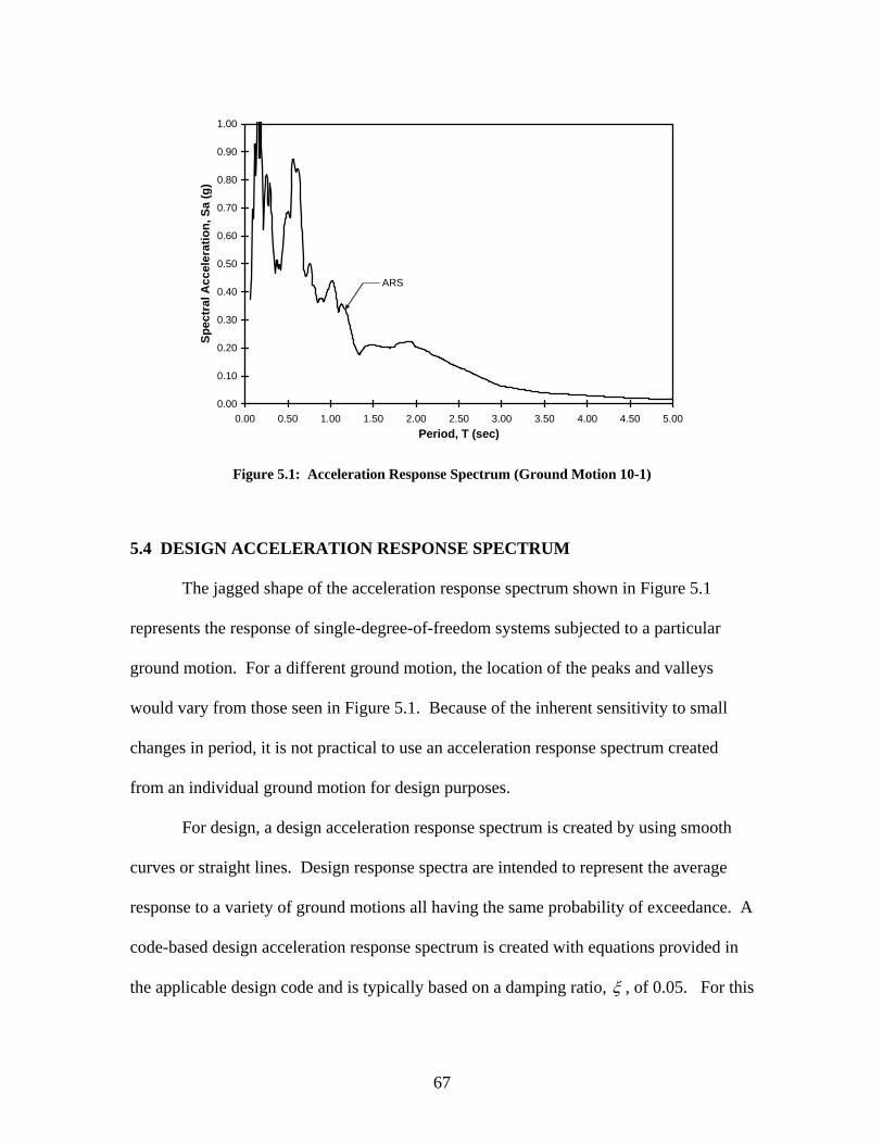
0.00
0.10
0.20
0.30
0.40
0.50
0.60
0.70
0.80
0.90
1.00
0.00 0.50 1.00 1.50 2.00 2.50 3.00 3.50 4.00 4.50 5.00Period, T (sec)
Spec
tral
Acc
eler
atio
n, S
a (g
)
ARS
Figure 5.1: Acceleration Response Spectrum (Ground Motion 10-1)
5.4 DESIGN ACCELERATION RESPONSE SPECTRUM
The jagged shape of the acceleration response spectrum shown in Figure 5.1
represents the response of single-degree-of-freedom systems subjected to a particular
ground motion. For a different ground motion, the location of the peaks and valleys
would vary from those seen in Figure 5.1. Because of the inherent sensitivity to small
changes in period, it is not practical to use an acceleration response spectrum created
from an individual ground motion for design purposes.
For design, a design acceleration response spectrum is created by using smooth
curves or straight lines. Design response spectra are intended to represent the average
response to a variety of ground motions all having the same probability of exceedance. A
code-based design acceleration response spectrum is created with equations provided in
the applicable design code and is typically based on a damping ratio, ξ , of 0.05. For this
67
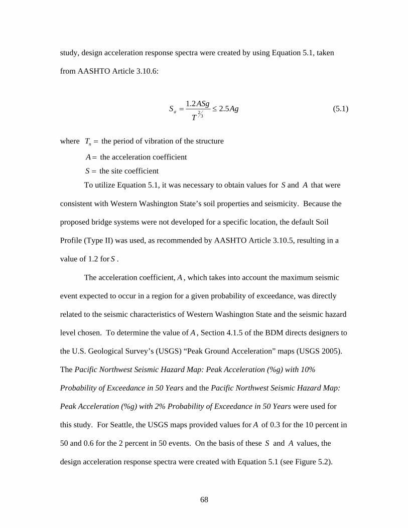
study, design acceleration response spectra were created by using Equation 5.1, taken
from AASHTO Article 3.10.6:
AgT
ASgSa 5.22.13
2 ≤= (5.1)
where the period of vibration of the structure nT =
A = the acceleration coefficient
S = the site coefficient
To utilize Equation 5.1, it was necessary to obtain values for and that were
consistent with Western Washington State’s soil properties and seismicity. Because the
proposed bridge systems were not developed for a specific location, the default Soil
Profile (Type II) was used, as recommended by AASHTO Article 3.10.5, resulting in a
value of 1.2 for .
S A
S
The acceleration coefficient, , which takes into account the maximum seismic
event expected to occur in a region for a given probability of exceedance, was directly
related to the seismic characteristics of Western Washington State and the seismic hazard
level chosen. To determine the value of , Section 4.1.5 of the BDM directs designers to
the U.S. Geological Survey’s (USGS) “Peak Ground Acceleration” maps (USGS 2005).
The Pacific Northwest Seismic Hazard Map: Peak Acceleration (%g) with 10%
Probability of Exceedance in 50 Years and the Pacific Northwest Seismic Hazard Map:
Peak Acceleration (%g) with 2% Probability of Exceedance in 50 Years were used for
this study. For Seattle, the USGS maps provided values for of 0.3 for the 10 percent in
50 and 0.6 for the 2 percent in 50 events. On the basis of these and values, the
design acceleration response spectra were created with Equation 5.1 (see Figure 5.2).
A
A
A
S A
68
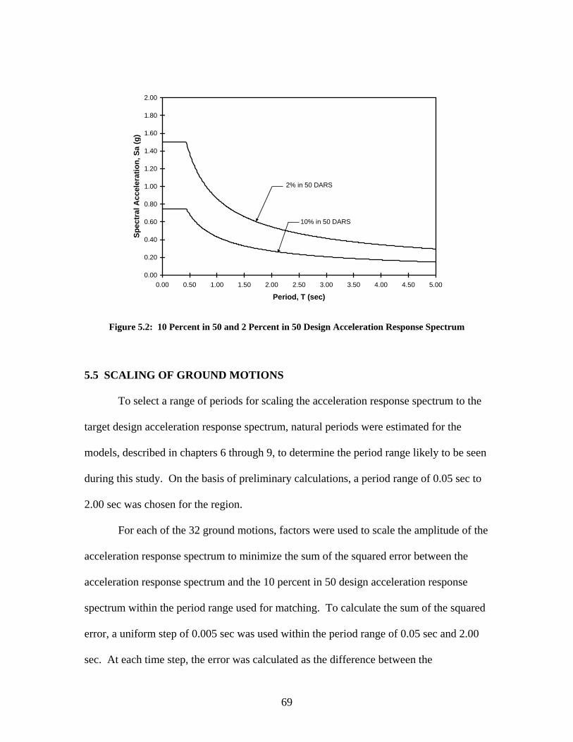
0.00
0.20
0.40
0.60
0.80
1.00
1.20
1.40
1.60
1.80
2.00
0.00 0.50 1.00 1.50 2.00 2.50 3.00 3.50 4.00 4.50 5.00
Period, T (sec)
Spec
tral
Acc
eler
atio
n, S
a (g
)
2% in 50 DARS
10% in 50 DARS
Figure 5.2: 10 Percent in 50 and 2 Percent in 50 Design Acceleration Response Spectrum
5.5 SCALING OF GROUND MOTIONS
To select a range of periods for scaling the acceleration response spectrum to the
target design acceleration response spectrum, natural periods were estimated for the
models, described in chapters 6 through 9, to determine the period range likely to be seen
during this study. On the basis of preliminary calculations, a period range of 0.05 sec to
2.00 sec was chosen for the region.
For each of the 32 ground motions, factors were used to scale the amplitude of the
acceleration response spectrum to minimize the sum of the squared error between the
acceleration response spectrum and the 10 percent in 50 design acceleration response
spectrum within the period range used for matching. To calculate the sum of the squared
error, a uniform step of 0.005 sec was used within the period range of 0.05 sec and 2.00
sec. At each time step, the error was calculated as the difference between the
69
acceleration response spectrum and the design acceleration response spectrum. This
value was then squared and added to the sum for the entire range used for matching. The
scale factor corresponding to the minimum sum of the squared error was referred to as
the motion’s scale factor.
Instead of performing the same procedure for the 2 percent in 50 event, it was
noted that the only difference between the 10 percent in 50 design acceleration response
spectrum and the 2 percent in 50 design acceleration response spectrum was that the
value for the 2 percent in 50 design acceleration response spectrum was twice as large as
the value for the 10 percent in 50 design acceleration response spectrum. Therefore, if
the same procedure was performed, the same ground motions would be chosen for the 2
percent in 50 event as were chosen for the 10 percent in 50 event, except with a scale
factor twice as large. On the basis of this observation, the same five motions selected for
the 10 percent in 50 event were also used for the 2 percent in 50 event, but with a scale
factor that was twice as large.
A
A
5.6 SELECTION OF GROUND MOTIONS
AASHTO specifications (Article 4.7.4.3.4) suggest that five ground motions be
considered for dynamic time history analysis when site-specific ground motions are not
available. This resulted in a ground motion suite containing ten ground motions: five 10
percent in 50 motions and five 2 percent in 50 motions.
With the ground motions scaled, it was possible to choose which of the 32 should
be included in the final ground motion suite. The five (of the 32) motions with the
smallest sum of the squared error were chosen unless individual ground motions were
eliminated on the basis of the following considerations. Smaller values of the sum of the
70
squared error were better than larger values because smaller values represented
acceleration response spectrum data that were closer to the design acceleration response
spectrum data. Individual ground motions were eliminated on the basis of the following
considerations:
• The final scale factor was noted to verify that it did not exceed 5.0. Because the
original scale factors for the ground motions (Woodward-Clyde Federal Services
1997) were scaled further during this study, the researchers felt that the ground
motion amplitude could become excessively distorted if the final scale factor
exceeded 5.0. The final scale factor was defined as the product of the original
scale and the scale factor from this study.
• Ground motions from the same component pair were not used. The original SAC
Suite ground motions contained 16 two-component histories; therefore, once one
component from a pair was selected for inclusion in the ground motion suite, the
other component was eliminated. This was done in an attempt to diversify the
time histories selected for the final suite.
• Finally, the time histories and the acceleration response spectra were reviewed
visually. Any ground motion or acceleration response spectrum that looked
unusual or did not adequately match the design acceleration response spectrum
was eliminated.
The ten ground motions selected for the suite are summarized in Table 5.1. The
scale factor tabulated is the final scale factor, as described above. The Peak Ground
Acceleration (PGA) shown is the PGA after all scaling was completed. Figure 5.3 shows
an example of a scaled time history and scaled acceleration response spectrum
71
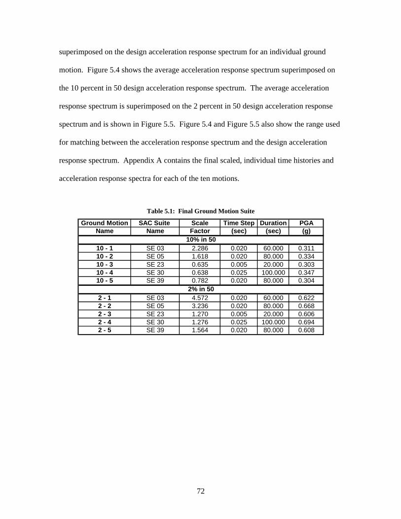
superimposed on the design acceleration response spectrum for an individual ground
motion. Figure 5.4 shows the average acceleration response spectrum superimposed on
the 10 percent in 50 design acceleration response spectrum. The average acceleration
response spectrum is superimposed on the 2 percent in 50 design acceleration response
spectrum and is shown in Figure 5.5. Figure 5.4 and Figure 5.5 also show the range used
for matching between the acceleration response spectrum and the design acceleration
response spectrum. Appendix A contains the final scaled, individual time histories and
acceleration response spectra for each of the ten motions.
Table 5.1: Final Ground Motion Suite
Ground Motion SAC Suite Scale Time Step Duration PGAName Name Factor (sec) (sec) (g)
10 - 1 SE 03 2.286 0.020 60.000 0.31110 - 2 SE 05 1.618 0.020 80.000 0.33410 - 3 SE 23 0.635 0.005 20.000 0.30310 - 4 SE 30 0.638 0.025 100.000 0.34710 - 5 SE 39 0.782 0.020 80.000 0.304
2 - 1 SE 03 4.572 0.020 60.000 0.6222 - 2 SE 05 3.236 0.020 80.000 0.6682 - 3 SE 23 1.270 0.005 20.000 0.6062 - 4 SE 30 1.276 0.025 100.000 0.6942 - 5 SE 39 1.564 0.020 80.000 0.608
10% in 50
2% in 50
72
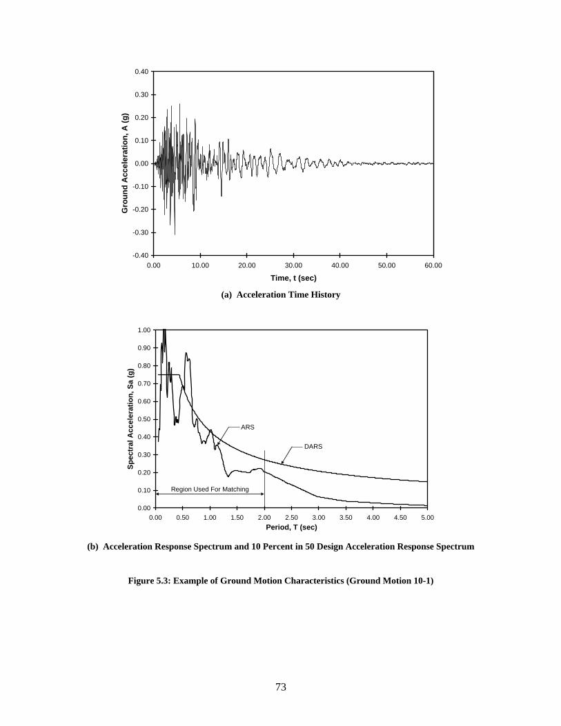
-0.40
-0.30
-0.20
-0.10
0.00
0.10
0.20
0.30
0.40
0.00 10.00 20.00 30.00 40.00 50.00 60.00
Time, t (sec)
Gro
und
Acc
eler
atio
n, A
(g)
(a) Acceleration Time History
0.00
0.10
0.20
0.30
0.40
0.50
0.60
0.70
0.80
0.90
1.00
0.00 0.50 1.00 1.50 2.00 2.50 3.00 3.50 4.00 4.50 5.00Period, T (sec)
Spec
tral
Acc
eler
atio
n, S
a (g
)
DARS
ARS
Region Used For Matching
(b) Acceleration Response Spectrum and 10 Percent in 50 Design Acceleration Response Spectrum
Figure 5.3: Example of Ground Motion Characteristics (Ground Motion 10-1)
73
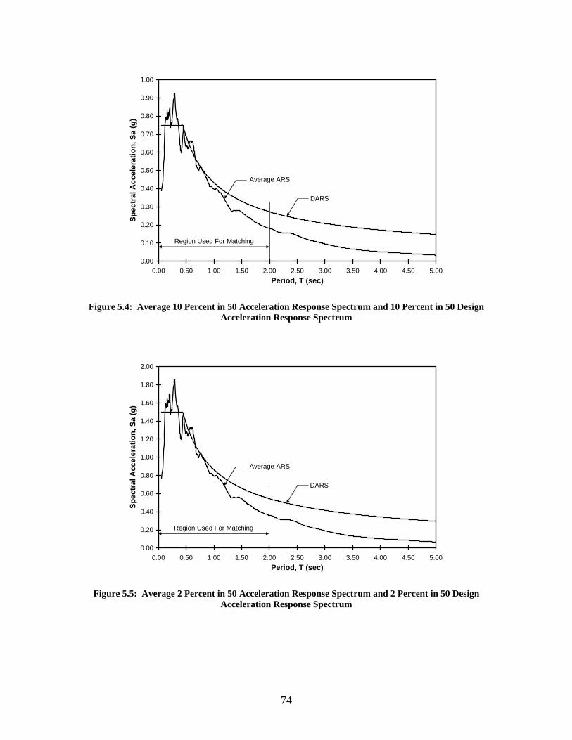
0.00
0.10
0.20
0.30
0.40
0.50
0.60
0.70
0.80
0.90
1.00
0.00 0.50 1.00 1.50 2.00 2.50 3.00 3.50 4.00 4.50 5.00Period, T (sec)
Spec
tral
Acc
eler
atio
n, S
a (g
)
DARS
Average ARS
Region Used For Matching
Figure 5.4: Average 10 Percent in 50 Acceleration Response Spectrum and 10 Percent in 50 Design Acceleration Response Spectrum
0.00
0.20
0.40
0.60
0.80
1.00
1.20
1.40
1.60
1.80
2.00
0.00 0.50 1.00 1.50 2.00 2.50 3.00 3.50 4.00 4.50 5.00Period, T (sec)
Spec
tral
Acc
eler
atio
n, S
a (g
)
DARS
Average ARS
Region Used For Matching
Figure 5.5: Average 2 Percent in 50 Acceleration Response Spectrum and 2 Percent in 50 Design Acceleration Response Spectrum
74
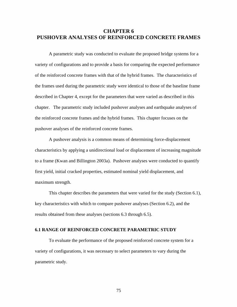
CHAPTER 6 PUSHOVER ANALYSES OF REINFORCED CONCRETE FRAMES
A parametric study was conducted to evaluate the proposed bridge systems for a
variety of configurations and to provide a basis for comparing the expected performance
of the reinforced concrete frames with that of the hybrid frames. The characteristics of
the frames used during the parametric study were identical to those of the baseline frame
described in Chapter 4, except for the parameters that were varied as described in this
chapter. The parametric study included pushover analyses and earthquake analyses of
the reinforced concrete frames and the hybrid frames. This chapter focuses on the
pushover analyses of the reinforced concrete frames.
A pushover analysis is a common means of determining force-displacement
characteristics by applying a unidirectional load or displacement of increasing magnitude
to a frame (Kwan and Billington 2003a). Pushover analyses were conducted to quantify
first yield, initial cracked properties, estimated nominal yield displacement, and
maximum strength.
This chapter describes the parameters that were varied for the study (Section 6.1),
key characteristics with which to compare pushover analyses (Section 6.2), and the
results obtained from these analyses (sections 6.3 through 6.5).
6.1 RANGE OF REINFORCED CONCRETE PARAMETRIC STUDY
To evaluate the performance of the proposed reinforced concrete system for a
variety of configurations, it was necessary to select parameters to vary during the
parametric study.
75
The results of the pushover analyses were normalized to reduce the number of
variables that required consideration. Suitable variables for use in the normalization
process can be selected by considering an idealized circular column in which the concrete
has no strength and in which the longitudinal reinforcement is elasto-plastic and is
uniformly distributed over the column’s cross-section. The horizontal resistance, , of
a two-column frame under fully plastic conditions is given as:
oH
322
32col
ocol
DHL
π ρ( )yf⎡ ⎤⎛ ⎞⎛ ⎞
= ⎢ ⎥⎜ ⎟⎜ ⎟⎢ ⎥⎝ ⎠⎝ ⎠⎣ ⎦
(6.1)
where column clear height between the top of the foundation and the bottom of the
cap-beam
colL =
colD = diameter of the column
ρ = longitudinal reinforcement ratio, s gA A
yf = longitudinal reinforcement yield strength, taken as 60 ksi
In this study, the normalized horizontal force, , was taken to be
proportional to
normalH
oH H , resulting in:
3 = colnormal
col y
HLHD fρ
(6.2)
where is the effective horizontal force on the force-displacement curve resulting from a
pushover analysis that considers second order
H
P − Δ effects.
Preliminary analyses were performed to determine the variables with the most
significant effect on pier performance. Figure 6.1 shows the normalized horizontal force,
, plotted against the drift ratio, normalH colLΔ , for column diameters equal to 36, 48, and
60 in. It is apparent from the figure that the column diameter only has a small influence
76
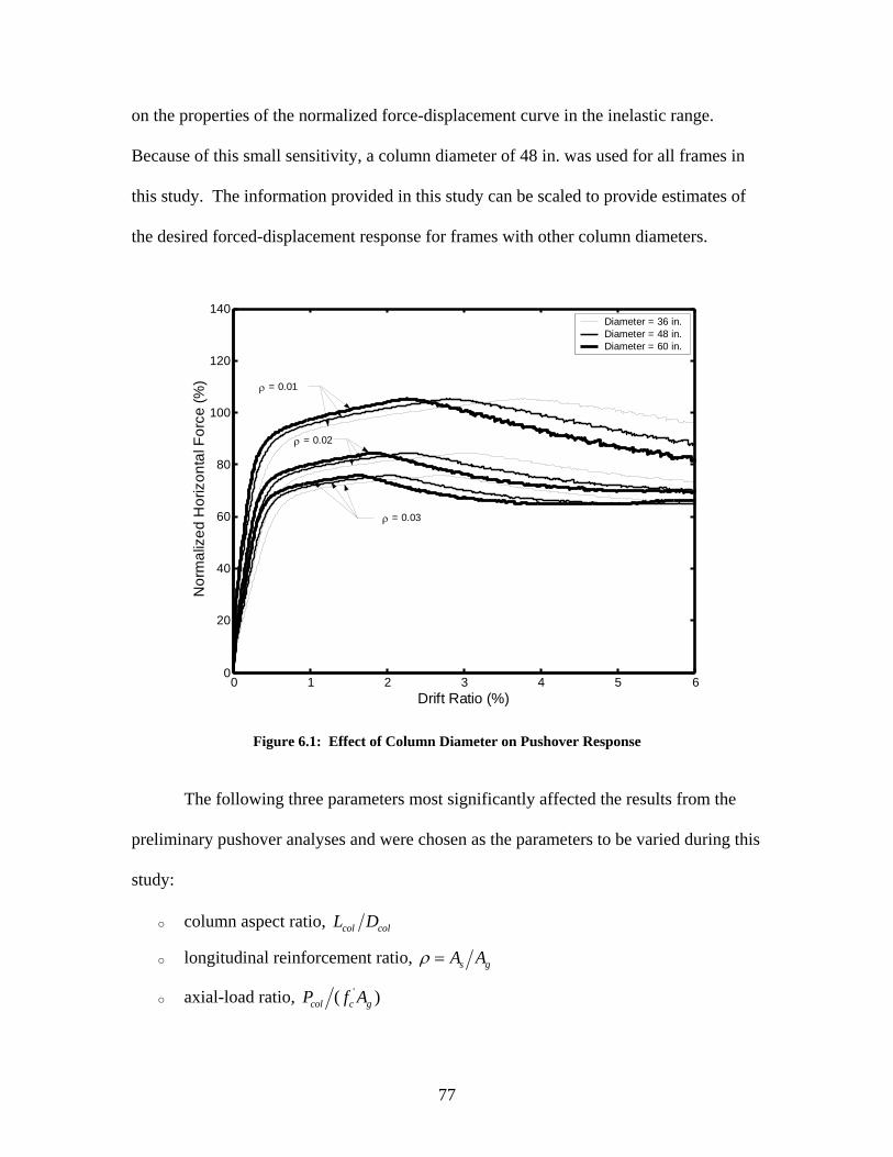
on the properties of the normalized force-displacement curve in the inelastic range.
Because of this small sensitivity, a column diameter of 48 in. was used for all frames in
this study. The information provided in this study can be scaled to provide estimates of
the desired forced-displacement response for frames with other column diameters.
0 1 2 3 4 5 60
20
40
60
80
100
120
140
Drift Ratio (%)
Nor
mal
ized
Hor
izon
tal F
orce
(%)
Diameter = 36 in.Diameter = 48 in.Diameter = 60 in.
ρ = 0.01
ρ = 0.02
ρ = 0.03
Figure 6.1: Effect of Column Diameter on Pushover Response
The following three parameters most significantly affected the results from the
preliminary pushover analyses and were chosen as the parameters to be varied during this
study:
o column aspect ratio, col colL D
o longitudinal reinforcement ratio, s gA Aρ =
o axial-load ratio, '( )col c gP f A
77
6.1.1 Column Aspect Ratio, col colL D
The column aspect ratio was defined as the length of the column divided by the
diameter of the column, col colL D .
The importance of including col colL D as one of the three parameters is evident by
considering an idealized circular column in which the concrete has no strength and in
which the longitudinal reinforcement is elastic and is uniformly distributed over the
column’s cross-section. Under elastic conditions the drift ratio, colLΔ , is proportional to
o col colH L D . The impacts of varying the column aspect ratio are seen in the results for
displacement and drift ratio corresponding to the states described in Chapter 10, the peak
displacement encountered during earthquake analyses, and the maximum strength.
Article 1120.04 (5) of the WSDOT Design Manual (WSDOT 2002 b) requires a
minimum vertical clearance of 16.5 ft for a bridge over a roadway. For a column
diameter of 48 in., this resulted in a minimum col colL D ratio of 4.125. This value was
increased to 5, 6, and 7 for the col colL D for this study.
6.1.2 Longitudinal Reinforcement Ratio, ρ
The longitudinal reinforcement ratio was defined as the area of the longitudinal
mild steel divided by the gross area of the column’s cross-section, s gA A . Section 9.2.1d
of the WSDOT Bridge Design Manual (WSDOT 2002a) provides an allowable range of
0.01 to 0.06 for a column’s longitudinal reinforcement ratio, ρ . Priestley et al. (1996)
also suggested a range of 0.005 to 0.04 for ρ with a practical design range of 0.01 to
0.03. The prototype frame described in Chapter 4 had a ρ value of 0.017.
78
On the basis of the allowable and suggested ranges, ρ values of 0.005, 0.01,
0.02, and 0.03 were chosen for this study, even though the ρ value of 0.005 does not fall
within the permissible range provided by the WSDOT Bridge Design Manual. This low
value was included to allow comparisons with the hybrid frames described in Chapter 8.
6.1.3 Axial-Load Ratio, '( )col c gP f A
The axial-load ratio was defined as the compressive axial-load on a column
divided by the product of the concrete compressive strength and the gross area of the
column’s cross-section, '( )col c gP f A . is the compressive axial-load for one column;
therefore, the two-column frame’s total load is two times . Article 5.10.11.4.1 b of the
AASHTO LRFD Bridge Design Specification (AASHTO 1998) permits axial-load ratios
of up to 0.20. The prototype bridge described in Chapter 4 had a
colP
colP
'(col c gP f A ) value of
approximately 0.075. Therefore, on the basis of AASHTO’s allowable range and the
prototype bridge, axial-load ratios of 0.05, 0.10, and 0.15 were selected for this study.
6.1.4 Frame Designation
Thirty-six unique combinations occurred as a result of varying these three
parameters. Frames were identified by the combination of their column aspect ratio,
longitudinal reinforcement ratio, and axial-load ratio. For example, 5.005.05 was a frame
with 5col colL D = , 0.005ρ = , and '( ) 0.05col c gP f A = ; 7.020.10 was a frame with
7col colL D = , 0.020ρ = , and '( ) 0.10col c gP f A = .
6.2 KEY CHARACTERISTICS OF PUSHOVER RESPONSE
This section describes the key characteristics that were calculated from the results
of the pushover analyses. These characteristics described the characteristics of the
79
individual frames as well as provided the basis for comparing the expected performance
of the reinforced concrete frames with that of the hybrid frames. Sections 6.4 through 6.6
discuss the results obtained from the analyses.
6.2.1 Uncracked Properties
The uncracked stiffness, , represented the tangent stiffness of the force-
displacement curve resulting from a pushover analysis. was established from an
eigenvalue analysis in OpenSees. The natural circular frequency of vibration,
uncrackedk
uncrackedk
nω , was
determined from the eigenvalue analysis of the frame before load was applied. From the
known quantity nω and the mass, , the uncracked stiffness was found from the
following relationship:
m
(6.3) 2
uncracked nk ω= m
The uncracked natural period, , was calculated from ,n uncrackedT nω with Equation
6.4.
,2
n uncrackedn
T πω
= (6.4)
6.2.2 First Yield
First yield was defined as the point at which the extreme tensile steel of the
column first reached its yield strain or the column concrete compressive strain reached
0.002, whichever occurred first. firstyieldF was defined as the effective force when first
yield occurred, and firstyieldΔ was defined as the corresponding displacement at first yield.
80
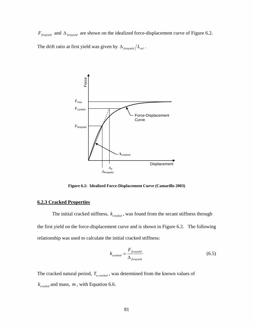
firstyieldF and firstyieldΔ are shown on the idealized force-displacement curve of Figure 6.2.
The drift ratio at first yield was given by firstyield colLΔ .
Fcon004
Ffirstyield
ΔyΔfirstyield
Force-Displacement Curve
kcracked
Forc
e
Displacement
Fmax
Figure 6.2: Idealized Force-Displacement Curve (Camarillo 2003)
6.2.3 Cracked Properties
The initial cracked stiffness, , was found from the secant stiffness through
the first yield on the force-displacement curve and is shown in Figure 6.2. The following
relationship was used to calculate the initial cracked stiffness:
crackedk
firstyieldcracked
firstyield
Fk =
Δ (6.5)
The cracked natural period, , was determined from the known values of
and mass, , with Equation 6.6.
,n crackedT
crackedk m
81
, 2n crackedcracked
mTk
π= (6.6)
6.2.4 Stiffness Ratio, cracked uncrackedk k
The stiffness ratio was defined as the cracked stiffness divided by the uncracked
stiffness. This ratio represented the loss of stiffness encountered as the force-
displacement relationship became nonlinear as a result of cracking in the concrete
columns.
6.2.5 Effective Force at Concrete Strain of 0.004, 004conF
004conF corresponded to the effective force when the concrete compressive strain
of 0.004 was first reached. It is illustrated in Figure 6.2.
6.2.6 Nominal Yield Displacement, yΔ
To calculate displacement ductility (Chapter 10), it was necessary to define a
yield displacement, . The loading applied during the pushover analyses resulted in
yielding of the frames and force-displacement curves that were nonlinear, as is seen in
Figure 6.2. As suggested by Priestley et al. (1996), the force-displacement curve was
idealized with an equivalent bilinear relationship by extrapolating up to to
obtain . The nominal yield displacement is shown in Figure 6.2 and was found with
the following relationship:
yΔ
crackedk 004conF
yΔ
004con firstyieldy
firstyield
FF
ΔΔ = (6.7)
82
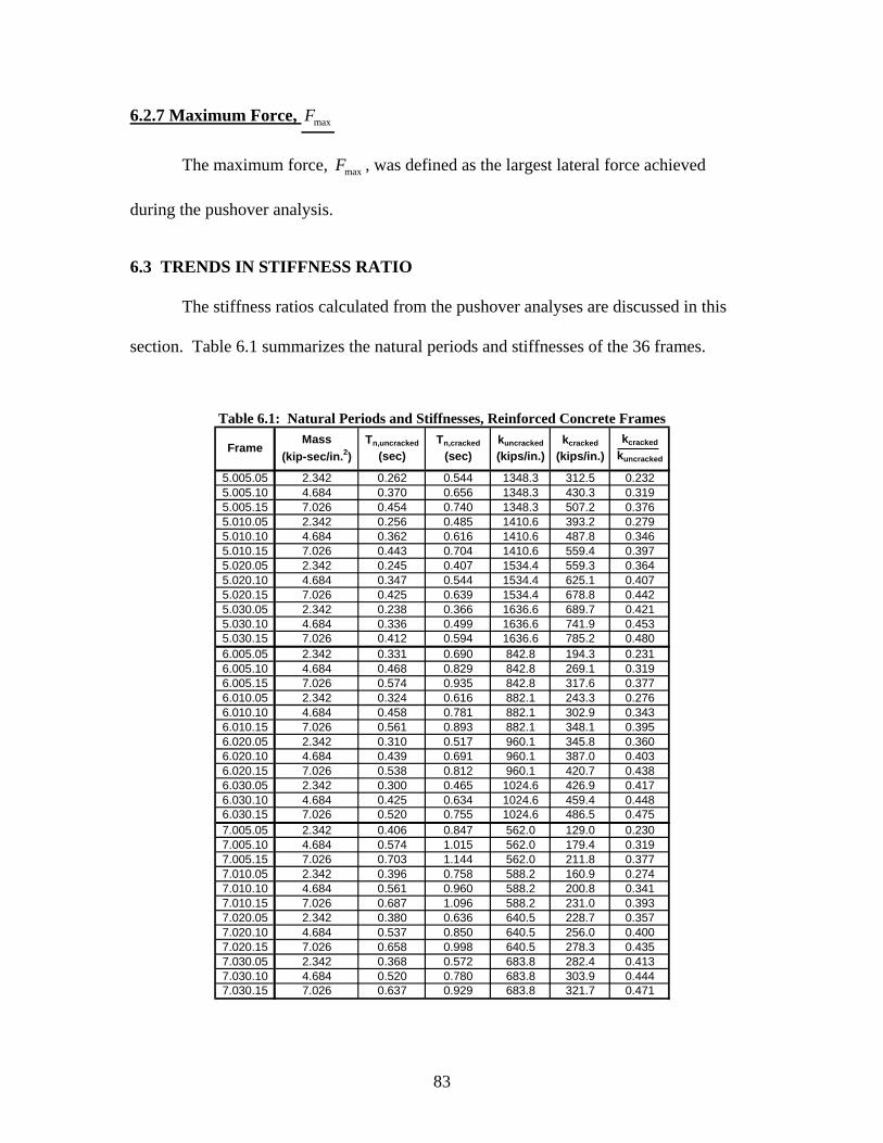
6.2.7 Maximum Force, maxF
The maximum force, , was defined as the largest lateral force achieved
during the pushover analysis.
maxF
6.3 TRENDS IN STIFFNESS RATIO
The stiffness ratios calculated from the pushover analyses are discussed in this
section. Table 6.1 summarizes the natural periods and stiffnesses of the 36 frames.
Table 6.1: Natural Periods and Stiffnesses, Reinforced Concrete Frames
5.005.05 2.342 0.262 0.544 1348.3 312.5 0.2325.005.10 4.684 0.370 0.656 1348.3 430.3 0.3195.005.15 7.026 0.454 0.740 1348.3 507.2 0.3765.010.05 2.342 0.256 0.485 1410.6 393.2 0.2795.010.10 4.684 0.362 0.616 1410.6 487.8 0.3465.010.15 7.026 0.443 0.704 1410.6 559.4 0.3975.020.05 2.342 0.245 0.407 1534.4 559.3 0.3645.020.10 4.684 0.347 0.544 1534.4 625.1 0.4075.020.15 7.026 0.425 0.639 1534.4 678.8 0.4425.030.05 2.342 0.238 0.366 1636.6 689.7 0.4215.030.10 4.684 0.336 0.499 1636.6 741.9 0.4535.030.15 7.026 0.412 0.594 1636.6 785.2 0.4806.005.05 2.342 0.331 0.690 842.8 194.3 0.2316.005.10 4.684 0.468 0.829 842.8 269.1 0.3196.005.15 7.026 0.574 0.935 842.8 317.6 0.3776.010.05 2.342 0.324 0.616 882.1 243.3 0.2766.010.10 4.684 0.458 0.781 882.1 302.9 0.3436.010.15 7.026 0.561 0.893 882.1 348.1 0.3956.020.05 2.342 0.310 0.517 960.1 345.8 0.3606.020.10 4.684 0.439 0.691 960.1 387.0 0.4036.020.15 7.026 0.538 0.812 960.1 420.7 0.4386.030.05 2.342 0.300 0.465 1024.6 426.9 0.4176.030.10 4.684 0.425 0.634 1024.6 459.4 0.4486.030.15 7.026 0.520 0.755 1024.6 486.5 0.4757.005.05 2.342 0.406 0.847 562.0 129.0 0.2307.005.10 4.684 0.574 1.015 562.0 179.4 0.3197.005.15 7.026 0.703 1.144 562.0 211.8 0.3777.010.05 2.342 0.396 0.758 588.2 160.9 0.2747.010.10 4.684 0.561 0.960 588.2 200.8 0.3417.010.15 7.026 0.687 1.096 588.2 231.0 0.3937.020.05 2.342 0.380 0.636 640.5 228.7 0.3577.020.10 4.684 0.537 0.850 640.5 256.0 0.4007.020.15 7.026 0.658 0.998 640.5 278.3 0.4357.030.05 2.342 0.368 0.572 683.8 282.4 0.4137.030.10 4.684 0.520 0.780 683.8 303.9 0.4447.030.15 7.026 0.637 0.929 683.8 321.7 0.471
kuncracked
(kips/in.)kcracked
(kips/in.)kcracked
kuncrackedFrame
Mass (kip-sec/in.2)
Tn,uncracked
(sec)Tn,cracked
(sec)
83
In Table 6.1, cracked uncrackedk k ranges from 0.23 to 0.48. These values are similar to
the values of 0.35 to 0.60 presented in Priestley et al. (1996) for typical circular
reinforced concrete columns with longitudinal reinforcement ratios of between 0.01 and
0.03 and axial load ratios of between 0.10 and 0.30. The lower cracked uncrackedk k range
observed during this study could be explained by smaller cracked stiffnesses resulting
from the bond model included in the frames and described in Lehman and Moehle
(2000).
The following trends were observed in the plots of cracked uncrackedk k shown in
Figure 6.3.
• cracked uncrackedk k increased as ρ increased. This trend is evident in Figure 6.3. For
example, cracked uncrackedk k increased by 81 percent between frames 5.005.05 and
5.030.05. Because was calculated from the transformed section,
increased as
uncrackedk
uncrackedk ρ increased. This was expected because the additional
theoretical transformed area of concrete (equal to snA where s cn E E= )
provided additional concrete area, resulting in an increased stiffness (Nawy
2000). also increased as crackedk ρ increased because the location of the neutral
axis depended on ρ , and therefore, as dictated by the principles of mechanics,
also depended on crackedk ρ (Nawy 2000). A change in ρ produced greater
variation in than in , as indicated by the increased crackedk uncrackedk cracked uncrackedk k
as ρ increased. Priestley et al. (1996) also found that cracked uncrackedk k increased
as ρ increased.
84
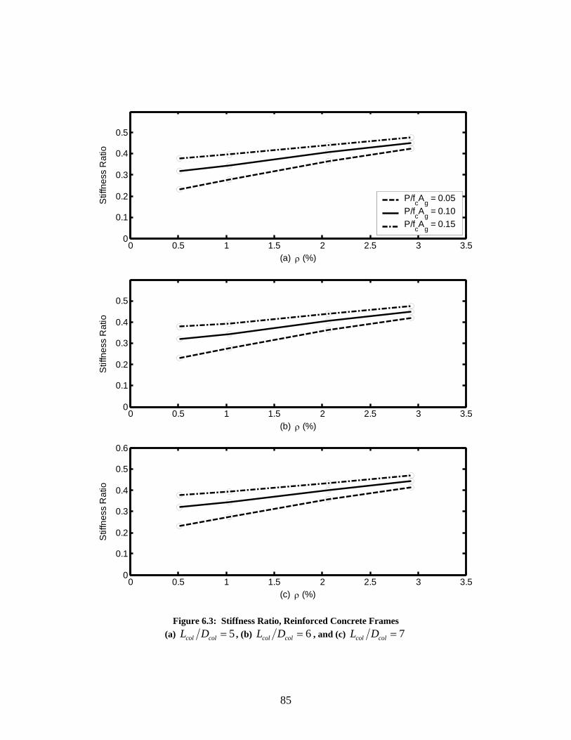
0 0.5 1 1.5 2 2.5 3 3.50
0.1
0.2
0.3
0.4
0.5
(a) ρ (%)
Stif
fnes
s R
atio
P/fcAg = 0.05P/fcAg = 0.10P/fcAg = 0.15
0 0.5 1 1.5 2 2.5 3 3.50
0.1
0.2
0.3
0.4
0.5
(b) ρ (%)
Stif
fnes
s R
atio
0 0.5 1 1.5 2 2.5 3 3.50
0.1
0.2
0.3
0.4
0.5
0.6
(c) ρ (%)
Stif
fnes
s R
atio
Figure 6.3: Stiffness Ratio, Reinforced Concrete Frames (a) 5col colL D = , (b) 6col colL D = , and (c) 7col colL D =
85
• cracked uncrackedk k increased as '(col c gP f A ) increased (Figure 6.3). The increase was
significantly larger for low values of ρ . An increase of 62 percent was observed
between frames 5.005.05 and 5.005.15, while an increase of only 14 percent was
observed between frames 5.030.05 and 5.030.15. '(col c gP f A ) had no influence
on but did affect . Before the section cracked, the stiffness was
based on the transformed gross section properties of the cross-section; therefore,
the axial-load on the column had no impact on the uncracked stiffness. After the
section cracked, as
uncrackedk crackedk
'(col c gP f A ) increased, the depth of the neutral axis also
increased, resulting in the increased cracked stiffness. Paulay and Priestley
(1992) provided recommended design values for cracked stiffness which indicate
larger values for larger axial-loads. Priestley et al. (1996) also found that
cracked uncrackedk k increased as '(col c gP f A ) increased for typical circular reinforced
concrete columns with longitudinal reinforcement ratios of between 0.01 and 0.03
and axial load ratios of between 0.10 and 0.30.
• As expected from the relationship for stiffness ( )3colk EI Lα= , both and
were affected by a variation in
uncrackedk
crackedk col colL D . cracked uncrackedk k remained
effectively unchanged as col colL D varied. This trend suggests that and
were similarly affected as
uncrackedk
crackedk col colL D varied.
In summary, ρ had the greatest influence on cracked uncrackedk k ; '(col c gP f A ) had a
moderate impact on cracked uncrackedk k ; and col colL D had almost no impact on
cracked uncrackedk k .
86
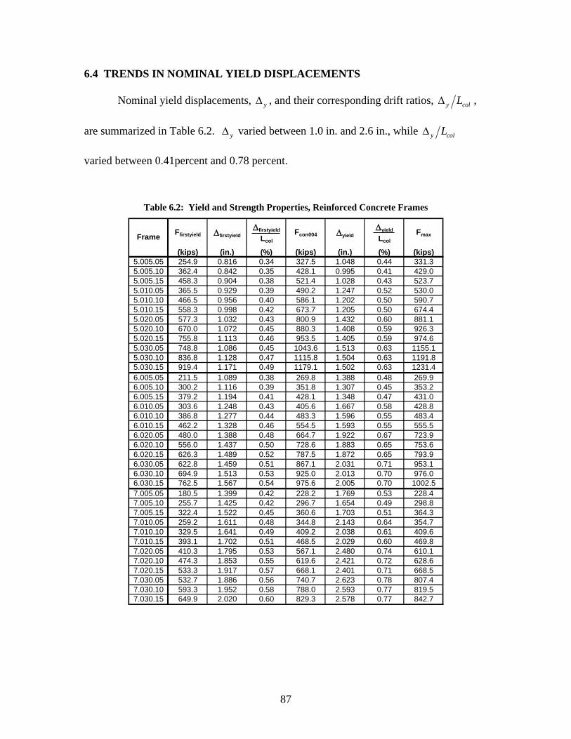
6.4 TRENDS IN NOMINAL YIELD DISPLACEMENTS
Nominal yield displacements, yΔ , and their corresponding drift ratios, y colLΔ ,
are summarized in Table 6.2. varied between 1.0 in. and 2.6 in., while yΔ y colLΔ
varied between 0.41percent and 0.78 percent.
Table 6.2: Yield and Strength Properties, Reinforced Concrete Frames
(kips) (in.) (%) (kips) (in.) (%) (kips)5.005.05 254.9 0.816 0.34 327.5 1.048 0.44 331.35.005.10 362.4 0.842 0.35 428.1 0.995 0.41 429.05.005.15 458.3 0.904 0.38 521.4 1.028 0.43 523.75.010.05 365.5 0.929 0.39 490.2 1.247 0.52 530.05.010.10 466.5 0.956 0.40 586.1 1.202 0.50 590.75.010.15 558.3 0.998 0.42 673.7 1.205 0.50 674.45.020.05 577.3 1.032 0.43 800.9 1.432 0.60 881.15.020.10 670.0 1.072 0.45 880.3 1.408 0.59 926.35.020.15 755.8 1.113 0.46 953.5 1.405 0.59 974.65.030.05 748.8 1.086 0.45 1043.6 1.513 0.63 1155.15.030.10 836.8 1.128 0.47 1115.8 1.504 0.63 1191.85.030.15 919.4 1.171 0.49 1179.1 1.502 0.63 1231.46.005.05 211.5 1.089 0.38 269.8 1.388 0.48 269.96.005.10 300.2 1.116 0.39 351.8 1.307 0.45 353.26.005.15 379.2 1.194 0.41 428.1 1.348 0.47 431.06.010.05 303.6 1.248 0.43 405.6 1.667 0.58 428.86.010.10 386.8 1.277 0.44 483.3 1.596 0.55 483.46.010.15 462.2 1.328 0.46 554.5 1.593 0.55 555.56.020.05 480.0 1.388 0.48 664.7 1.922 0.67 723.96.020.10 556.0 1.437 0.50 728.6 1.883 0.65 753.66.020.15 626.3 1.489 0.52 787.5 1.872 0.65 793.96.030.05 622.8 1.459 0.51 867.1 2.031 0.71 953.16.030.10 694.9 1.513 0.53 925.0 2.013 0.70 976.06.030.15 762.5 1.567 0.54 975.6 2.005 0.70 1002.57.005.05 180.5 1.399 0.42 228.2 1.769 0.53 228.47.005.10 255.7 1.425 0.42 296.7 1.654 0.49 298.87.005.15 322.4 1.522 0.45 360.6 1.703 0.51 364.37.010.05 259.2 1.611 0.48 344.8 2.143 0.64 354.77.010.10 329.5 1.641 0.49 409.2 2.038 0.61 409.67.010.15 393.1 1.702 0.51 468.5 2.029 0.60 469.87.020.05 410.3 1.795 0.53 567.1 2.480 0.74 610.17.020.10 474.3 1.853 0.55 619.6 2.421 0.72 628.67.020.15 533.3 1.917 0.57 668.1 2.401 0.71 668.57.030.05 532.7 1.886 0.56 740.7 2.623 0.78 807.47.030.10 593.3 1.952 0.58 788.0 2.593 0.77 819.57.030.15 649.9 2.020 0.60 829.3 2.578 0.77 842.7
Fcon004 ΔyieldΔyield
LcolFmaxFfirstyield Δfirstyield
Δfirstyield
LcolFrame
87
The following trends are evident from the plots of yΔ and y colLΔ shown in
Figure 6.4. The trends are discussed for y colLΔ , but similar trends were seen in ,
although the variations observed in the
yΔ
y colLΔ trends were significantly larger than
those for . yΔ
• y colLΔ increased as ρ increased, as shown in Figure 6.4. For example, y colLΔ
increased by 43 percent between frames 5.005.05 and 5.030.05. This trend can be
explained by investigating the change in stiffness and strength between frames
5.005.05 and 5.030.05. The ratio of between the two frames was equal to
0.45, whereas the ratio of between the two frames was 0.31. Because the
increase in strength was greater than the increase in stiffness, it would be
expected, given geometry, that
crackedk
004conF
y colLΔ would also increase. From Table 6.2 it is
also clear that the displacement at first yield also increased as ρ increased. This
trend is explained by examining flexure of a square cross-section with a width
equal to . The neutral-axis, c , is directly related to the amount of steel in the
section, as shown by the relationship
b
( ) ( )'g y cc A f f bρ= 0.85β , where yf is the
yield strength of the longitudinal mild steel, 'cf is the concrete compressive
strength, and β is the stress block depth factor. Mechanics dictate that as the
neutral-axis increases the curvature increases, and accordingly, the displacement
at first yield also increases.
88
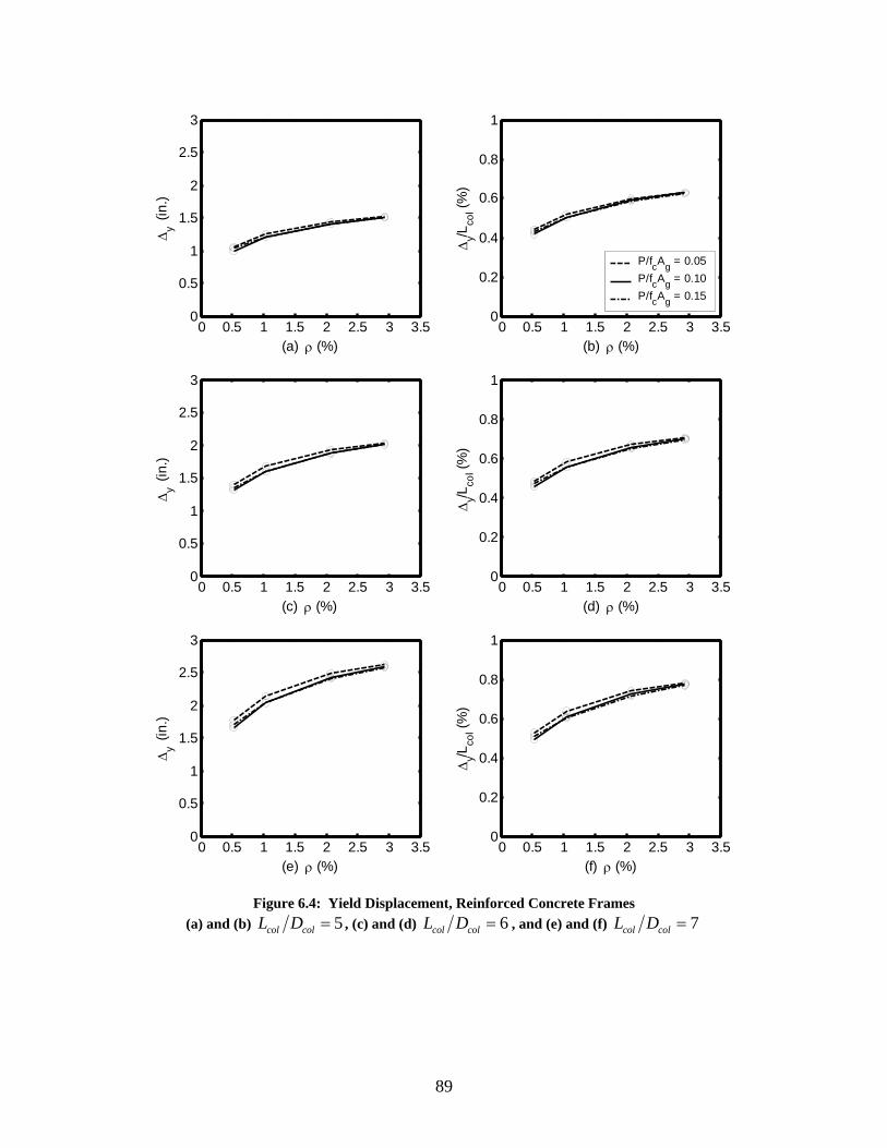
0 0.5 1 1.5 2 2.5 3 3.50
0.5
1
1.5
2
2.5
3
(a) ρ (%)
Δy (
in.)
0 0.5 1 1.5 2 2.5 3 3.50
0.5
1
1.5
2
2.5
3
(c) ρ (%)
Δy (
in.)
0 0.5 1 1.5 2 2.5 3 3.50
0.5
1
1.5
2
2.5
3
(e) ρ (%)
Δy (
in.)
0 0.5 1 1.5 2 2.5 3 3.50
0.2
0.4
0.6
0.8
1
(b) ρ (%)
Δy/L
col (%
)
P/fcAg = 0.05P/fcAg = 0.10P/fcAg = 0.15
0 0.5 1 1.5 2 2.5 3 3.50
0.2
0.4
0.6
0.8
1
(d) ρ (%)
Δy/L
col (%
)
0 0.5 1 1.5 2 2.5 3 3.50
0.2
0.4
0.6
0.8
1
(f) ρ (%)
Δy/L
col (%
)
Figure 6.4: Yield Displacement, Reinforced Concrete Frames (a) and (b) 5col colL D = , (c) and (d) 6col colL D = , and (e) and (f) 7col colL D =
89
• Figure 6.4 indicates that y colLΔ remained essential unchanged as '( )col c gP f A
increased. An increase was not observed in these results because
'(col c gP f A ) similarly influenced cracked stiffness and strength. For example, the
ratio of between frames 5.030.05 and 5.030.15 was 0.87 (Table 6.1) and
the ratio of was also 0.87 (Table 6.2). Paulay and Priestley (1992)
suggested that as the axial-load increases, the yield displacement should also
increase.
crackedk
004conF
• y colLΔ increased as col colL D increased (Figure 6.4). A 22 percent increase was
seen between frames 5.030.15 and 7.030.15. This trend is explained by the
decreased cracked stiffness as col colL D increased.
These trends indicate that ρ had the greatest influence on y colLΔ ; col colL D had
a moderate impact on y colLΔ ; and '(col c gP f A ) effectively had no influence on y colLΔ .
For , the largest impact was caused by yΔ col colL D .
6.5 TRENDS IN MAXIMUM FORCE
As shown in Table 6.2, ranged from 228 to 1231 kips. The large values
corresponded to a short column, with a large
maxF
ρ and '(col c gP f A ) , while the small values
corresponded to a tall column, with a small ρ and '(col c gP f A ) . The following trends
were observed in the results, shown in Figure 6.5.
90
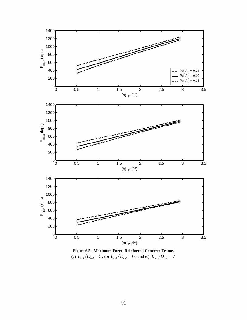
0 0.5 1 1.5 2 2.5 3 3.50
200
400
600
800
1000
1200
1400
(a) ρ (%)
F max
(kip
s)
P/fcAg = 0.05P/fcAg = 0.10P/fcAg = 0.15
0 0.5 1 1.5 2 2.5 3 3.50
200
400
600
800
1000
1200
1400
(b) ρ (%)
F max
(kip
s)
0 0.5 1 1.5 2 2.5 3 3.50
200
400
600
800
1000
1200
1400
(c) ρ (%)
F max
(kip
s)
Figure 6.5: Maximum Force, Reinforced Concrete Frames
(a) 5col colL D = , (b) 6col colL D = , and (c) 7col colL D =
91
• The maximum force, , increased as maxF ρ increased. An increase of 250 percent
was observed between frames 5.005.05 and 5.030.05. The flexural strength of a
column is directly related to the quantity of longitudinal reinforcing steel
provided. Therefore, this trend can be attributed to an increased flexural strength
provided by the increased steel.
• increased asmaxF '(col c gP f A ) increased, as is evident in Figure 6.5. The increase
was significantly larger for low values of ρ . An increase of 58 percent was
observed between frames 5.005.05 and 5.005.15, whereas an increase of only 7
percent was observed between frames 5.030.05 and 5.030.15. The '( )col c gP f A
on bridge columns is normally around 0.10, which is relatively low. As a result,
typical bridge columns fall below the balanced failure point on a column
interaction diagram. Below the balanced failure point, an increase in compressive
axial-load results in an increase in flexural strength, which corresponds with the
trend observed.
• decreased as maxF col colL D increased (Figure 6.5). For example, a decrease of 32
percent was observed between frames 5.030.15 and 7.030.15. As col colL D
increased, the cracked stiffness decreased, resulting in the decreased . maxF
These trends indicate that ρ had the greatest influence on ; maxF '(col c gP f A ) had a
varying impact on ; and maxF col colL D had the least influence on . maxF
92
CHAPTER 7 EARTHQUAKE ANALYSES
OF REINFORCED CONCRETE FRAMES
A parametric study was conducted to evaluate the proposed bridge systems
described in Chapter 3 and provide a basis for comparison between the expected
performance of the reinforced concrete frames and that of the hybrid frames. The
parametric study included pushover analyses and earthquake analyses of the reinforced
concrete frames and the hybrid frames.
This chapter addresses the earthquake analyses of the reinforced concrete frames
that were conducted to quantify maximum displacements and residual displacements
resulting from the 10 ground motions described in Chapter 5. The 10 ground motions
included five ground motions with a 10 percent probability of exceedance in 50 years (10
percent in 50) and five ground motions with a 2 percent probability of exceedance in 50
years (2 percent in 50). This chapter describes the parameters that were varied for the
study (Section 7.1), key characteristics used to compare earthquake analyses (Section
7.2), and the results obtained from these analyses (sections 7.3 through 7.7).
7.1 RANGE OF REINFORCED CONCRETE PARAMETRIC STUDY
The analyses were conducted on variations of the baseline frame described in
Chapter 4. On the basis of preliminary pushover analyses, the following three parameters
were varied, as described in Chapter 6:
o column aspect ratio, col colL D
o longitudinal reinforcement ratio, s gA Aρ =
o axial-load ratio, '( )col c gP f A .
93
7.2 KEY CHARACTERISTICS OF EARTHQUAKE RESPONSE
This section describes the key characteristics that were calculated from the results
of the earthquake analyses. These characteristics describe the response of the frames to
the earthquake analyses and provide a basis for comparison between the reinforced
frames and the hybrid frames. Sections 7.3 through 7.7 discuss the results obtained from
the earthquake analyses of the reinforced concrete frames.
7.2.1 Maximum Displacement, maxΔ
The maximum displacement, maxΔ , was defined as the maximum absolute value
displacement encountered during an earthquake analysis. The maximum displacement
can provide insight into the likelihood that a particular frame/ground motion combination
will result in spalling, bar buckling, or the occurrence of the ultimate limit state, as
described in Chapter 10. The maximum displacement was also used to calculate the
displacement ductility demand on the frame. The displacement ductility demand is a
useful measure for comparing the earthquake response of different frames and will be
explained in Chapter 10. The corresponding drift ratio at the maximum displacement was
given as max colLΔ .
7.2.2 Residual Displacement, residualΔ
The residual displacement, residualΔ , was defined as the displacement from the
frame’s initial equilibrium position after the ground motion excitation had ended. After
an inelastic system has yielded, it may not vibrate around its original equilibrium
position. With each subsequent occurrence of yielding, the system may shift to another
location about which it will oscillate. Therefore, after the ground excitation has ended, a
94
frame that has yielded will typically not return to its original equilibrium point, resulting
in a residual displacement (Chopra 2001).
For this study, the residual displacements were found by considering the free
vibration of the frame after the ground motion had stopped. This was done because no
viscous damping was included in the frame. The residual displacements were estimated
by averaging the maximum and minimum displacements over a time range starting 4 sec.
after the ground excitation had stopped, , 4set stop+ cΔ , and ending 9 sec. after the ground
excitation had stopped, . The residual displacements were calculated from the
following relationship:
, 9set stop+Δ c
, 4sec , 9sec , 4sec , 9semax( ) min( )2.0
t stop t stop t stop t stopresidual
+ + +Δ → Δ + Δ → ΔΔ = c+ (7.1)
7.3 TRENDS IN MAXIMUM DISPLACEMENT
This section discusses the maximum displacements encountered during the
earthquake analyses. Tables B.1 and B.2, found in Appendix B, provide a complete
summary of the maximum displacements for individual ground motions and mean values
for both the 10 percent in 50 and 2 percent in 50 motions.
For the 2 percent in 50 ground motions, ten frame/ground motion combinations
had a displacement of over 100 in., with OpenSees encountering convergence problems
with each occurrence. It is difficult to say whether the convergence problems caused the
extreme displacements, or the extreme displacements caused the convergence problems.
For this study, these values were omitted when mean values were calculated. Eight of the
10 convergence problems occurred as a result of ground motion 2-3. The other two
95
convergence problems occurred with frame 5.005.15. The frames that had convergence
problems had small longitudinal reinforcement ratios and large axial-load ratios.
For the 10 percent in 50 ground motions, the extreme values of the maximum
displacement ranged from a minimum of 0.9 in. (frame 6.030.05, ground motion 10-3,
max colLΔ = 0.33 percent) to a maximum of 10.7 in. (frame 7.005.15, ground motion 10-3,
max colLΔ = 3.19 percent). For the 2 percent in 50 ground motions, the maximum
displacement ranged from a minimum of 1.9 in. (frame 5.030.05, ground motion 2-1,
max colLΔ = 0.79 percent) to a maximum of 28.4 in. (frame 7.005.10, ground motion 2-3,
max colLΔ = 8.47 percent).
The same frame, frame 5.030.05, resulted in the minimum average displacement
when subjected to the 10 percent in 50 ground motions (1.6 in.) and the 2 percent in 50
ground motions (2.3 in.). This was not the case with the maximum average displacement.
Instead, frame 7.005.15 resulted in the largest average displacement for the 10 percent in
50 ground motions (7.7 in.), whereas frame 7.005.10 resulted in the largest average
displacement for the 2 percent in 50 ground motions (14.9 in.). This inconsistency is a
consequence of omitting the 10 frames that experienced convergence problems. With the
2 percent in 50 ground motions, motion 2-3 caused the largest displacement for each of
the frames. Therefore, by omitting this motion’s contribution to the average
displacement for frame 7.005.15, frame 7.005.10 had a larger average displacement.
Figure 7.1 shows the mean and the mean plus one standard deviation maximum
drift ratio for the 2 percent in 50 ground motions. Because the general trends observed in
the maximum drift ratio were similar for the 2 percent in 50 ground motions and the 10
percent ground motions, only figures showing the results for the 2 percent in 50 ground
96
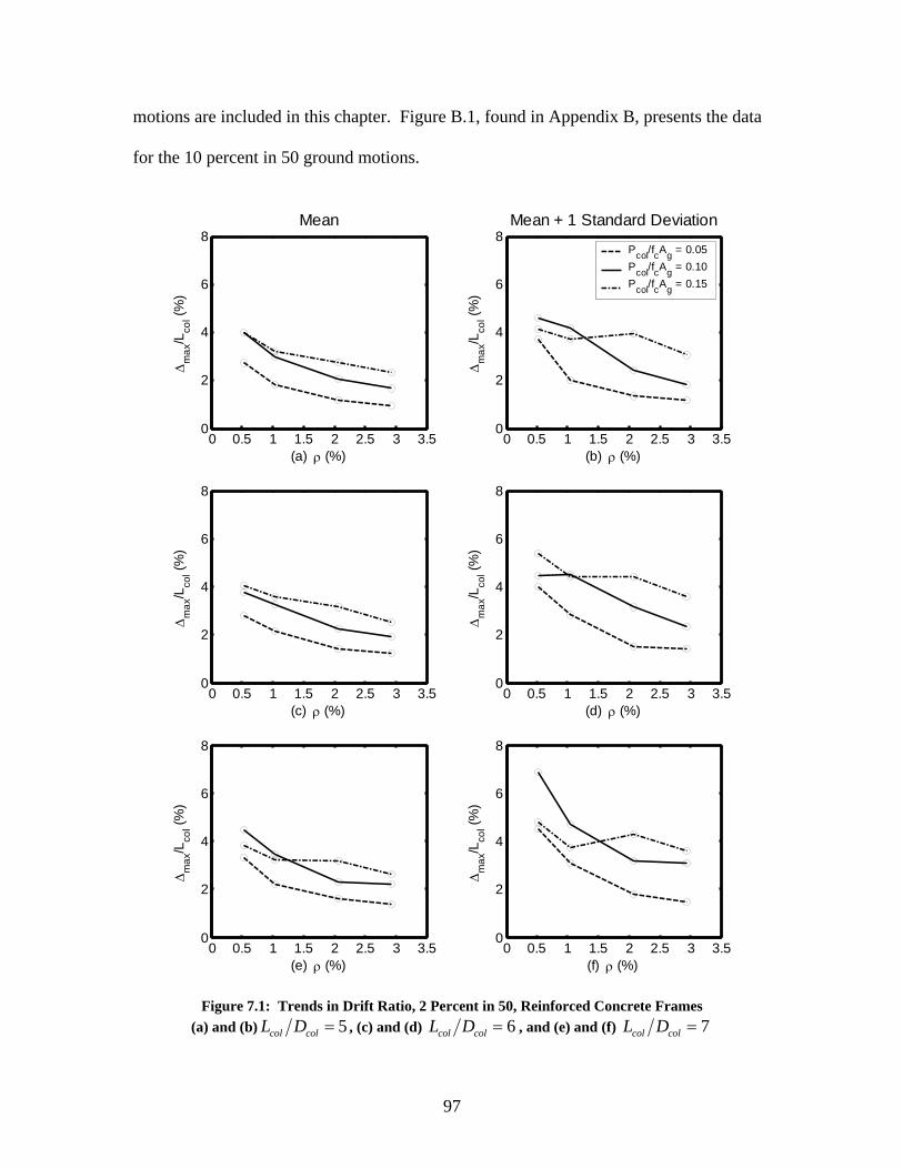
motions are included in this chapter. Figure B.1, found in Appendix B, presents the data
for the 10 percent in 50 ground motions.
0 0.5 1 1.5 2 2.5 3 3.50
2
4
6
8
(a) ρ (%)
Δm
ax/L
col (%
)
Mean
0 0.5 1 1.5 2 2.5 3 3.50
2
4
6
8
(c) ρ (%)
Δm
ax/L
col (%
)
0 0.5 1 1.5 2 2.5 3 3.50
2
4
6
8
(e) ρ (%)
Δm
ax/L
col (%
)
0 0.5 1 1.5 2 2.5 3 3.50
2
4
6
8
(b) ρ (%)Δ
max
/Lco
l (%)
Mean + 1 Standard Deviation
Pcol/fcAg = 0.05Pcol/fcAg = 0.10Pcol/fcAg = 0.15
0 0.5 1 1.5 2 2.5 3 3.50
2
4
6
8
(d) ρ (%)
Δm
ax/L
col (%
)
0 0.5 1 1.5 2 2.5 3 3.50
2
4
6
8
(f) ρ (%)
Δm
ax/L
col (%
)
Figure 7.1: Trends in Drift Ratio, 2 Percent in 50, Reinforced Concrete Frames (a) and (b) 5col colL D = , (c) and (d) 6col colL D = , and (e) and (f) 7col colL D =
97
The results presented in Figure 7.1 display the following trends. The trends are
discussed for the mean drift ratio, but the trends are also reflected in the responses from
each individual ground motion. The inconsistencies described in the preceding paragraph
are reflected in Figure 7.1 at the locations where the lines cross one another.
• max colLΔ decreased as ρ increased, as is indicated in Figure 7.1. For example,
the drift ratio decreased by 60 percent between frames as the reinforcement ratio
increased from 0.005 to 0.030. From the results of the pushover analyses
(Chapter 6), it was evident that a frame’s strength and cracked stiffness increased
as ρ increased. This increased strength, as well as cracked stiffness, resulted in a
decreased max colLΔ encountered during the earthquake analyses.
• max colLΔ increased as '(col c gP f A ) increased. The drift ratio increased on average
by 100 percent as the axial-load ratio increased from 0.05 to 0.15. This
observation can be explained by considering the increased mass corresponding to
an increased '(col c gP f A ) . The mass applied to the frame was equal to
compressive axial-load on the column divided by gravity. Given the relationship
for the cracked natural period ( ),n cracked crackedT m k= , it is evident that as mass
increased, the cracked natural period also increased. The displacement response
spectrum shown later in this chapter indicates that an increase in should
result in an increase in the predicted displacement. The cracked natural period
may also have increased further because the increased mass reduced the cracked
stiffness as a result of the
,n crackedT
P − Δ effect.
98
• max colLΔ was only slightly influenced by col colL D . This observation is apparent
from the data presented in Figure 7.1. An increase of 14 percent was observed
between 5.030.15 and 7.030.15. The results of the pushover analyses of the
reinforced concrete frames indicated that as col colL D increased the frame
stiffness decreased. The increased max colLΔ resulted from the decreased stiffness.
The impact of col colL D is more significant when the results for the average maxΔ
are examined instead of max colLΔ . For example, maxΔ increased 60 percent
between frames 5.030.15 and 7.030.15.
• Figure 7.1 indicates that the mean plus one stand deviation was approximately 50
percent larger than the mean values.
• The results for max colLΔ from the 2 percent in 50 ground motions were about 50
percent larger than the results for the 10 percent in 50 ground motions. The
graphs in Figure B.1 in Appendix B illustrate the data for the maximum drift ratio
resulting from the 10 percent in 50 ground motions.
These trends indicate that the '(col c gP f A ) had the greatest influence on max colLΔ ;
ρ had a moderate impact; and col colL D had the least impact on max colLΔ . As explained
above, col colL D had a more significant impact on maxΔ than it did on max colLΔ .
7.4 EFFECTS OF STRENGTH ON MAXIMUM DISPLACEMENT
This section examines other quantities that affected the resulting maximum
displacement. To evaluate the impact of strength on maximum displacement, the
maximum drift ratio, max colLΔ , was plotted against the normalized force 004con totalF P ,
99
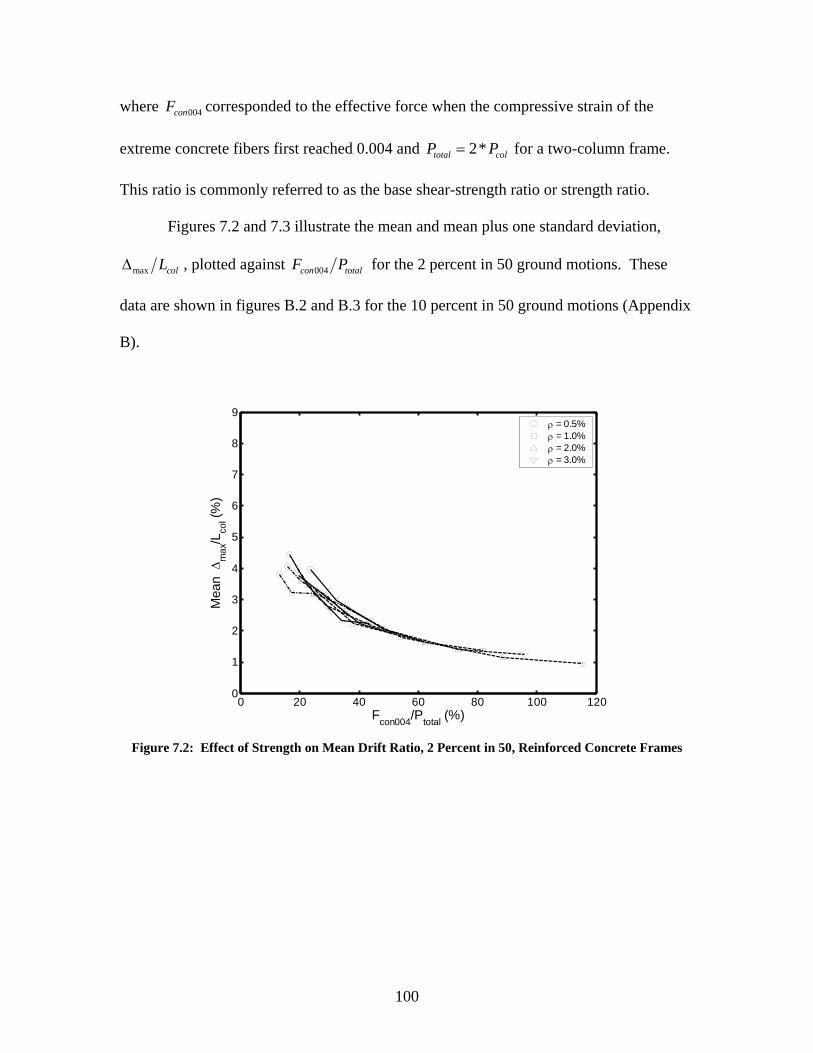
where corresponded to the effective force when the compressive strain of the
extreme concrete fibers first reached 0.004 and
004conF
2*total colP P= for a two-column frame.
This ratio is commonly referred to as the base shear-strength ratio or strength ratio.
Figures 7.2 and 7.3 illustrate the mean and mean plus one standard deviation,
max colLΔ , plotted against 004con totalF P for the 2 percent in 50 ground motions. These
data are shown in figures B.2 and B.3 for the 10 percent in 50 ground motions (Appendix
B).
0 20 40 60 80 100 1200
1
2
3
4
5
6
7
8
9
Fcon004/Ptotal (%)
Mea
n Δ
max
/Lco
l (%)
ρ = 0.5%ρ = 1.0%ρ = 2.0%ρ = 3.0%
Figure 7.2: Effect of Strength on Mean Drift Ratio, 2 Percent in 50, Reinforced Concrete Frames
100
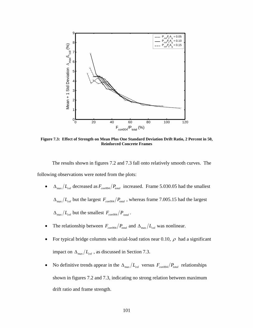
0 20 40 60 80 100 1200
1
2
3
4
5
6
7
8
9
Fcon004/Ptotal (%)
Mea
n +
1 S
td D
evia
tion
Δm
ax/L
col (%
)
Pcol/fcAg = 0.05Pcol/fcAg = 0.10Pcol/fcAg = 0.15
Figure 7.3: Effect of Strength on Mean Plus One Standard Deviation Drift Ratio, 2 Percent in 50, Reinforced Concrete Frames
The results shown in figures 7.2 and 7.3 fall onto relatively smooth curves. The
following observations were noted from the plots:
• max colLΔ decreased as 004con totalF P increased. Frame 5.030.05 had the smallest
max colLΔ but the largest 004con totalF P , whereas frame 7.005.15 had the largest
max colLΔ but the smallest 004con totalF P .
• The relationship between 004con totalF P and max colLΔ was nonlinear.
• For typical bridge columns with axial-load ratios near 0.10, ρ had a significant
impact on max colLΔ , as discussed in Section 7.3.
• No definitive trends appear in the max colLΔ versus 004con totalF P relationships
shown in figures 7.2 and 7.3, indicating no strong relation between maximum
drift ratio and frame strength.
101
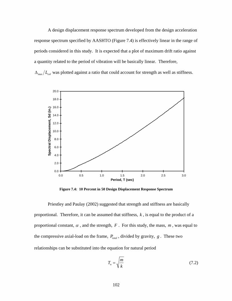
A design displacement response spectrum developed from the design acceleration
response spectrum specified by AASHTO (Figure 7.4) is effectively linear in the range of
periods considered in this study. It is expected that a plot of maximum drift ratio against
a quantity related to the period of vibration will be basically linear. Therefore,
max colLΔ was plotted against a ratio that could account for strength as well as stiffness.
0.0
2.0
4.0
6.0
8.0
10.0
12.0
14.0
16.0
18.0
20.0
0.0 0.5 1.0 1.5 2.0 2.5Period, T (sec)
Spec
tral
Dis
plac
emen
t, Sd
(in.
)
3.0
Figure 7.4: 10 Percent in 50 Design Displacement Response Spectrum
Priestley and Paulay (2002) suggested that strength and stiffness are basically
proportional. Therefore, it can be assumed that stiffness, , is equal to the product of a
proportional constant,
k
α , and the strength, . For this study, the mass, , was equal to
the compressive axial-load on the frame, , divided by gravity, . These two
relationships can be substituted into the equation for natural period
F m
totalP g
nmTk
= (7.2)
102
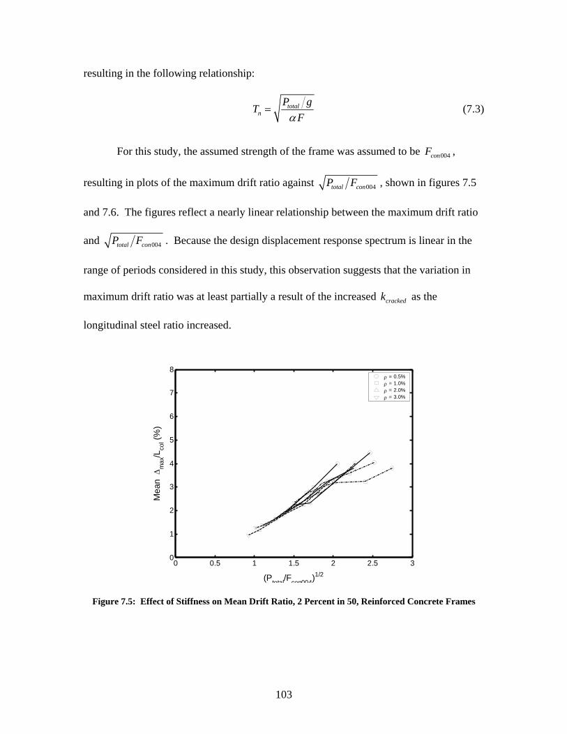
resulting in the following relationship:
totaln
P gTFα
= (7.3)
For this study, the assumed strength of the frame was assumed to be ,
resulting in plots of the maximum drift ratio against
004conF
004total conP F , shown in figures 7.5
and 7.6. The figures reflect a nearly linear relationship between the maximum drift ratio
and 004total conP F . Because the design displacement response spectrum is linear in the
range of periods considered in this study, this observation suggests that the variation in
maximum drift ratio was at least partially a result of the increased as the
longitudinal steel ratio increased.
crackedk
0 0.5 1 1.5 2 2.5 30
1
2
3
4
5
6
7
8
(Ptotal/Fcon004)1/2
Mea
n Δ
max
/Lco
l (%)
ρ = 0.5%ρ = 1.0%ρ = 2.0%ρ = 3.0%
Figure 7.5: Effect of Stiffness on Mean Drift Ratio, 2 Percent in 50, Reinforced Concrete Frames
103
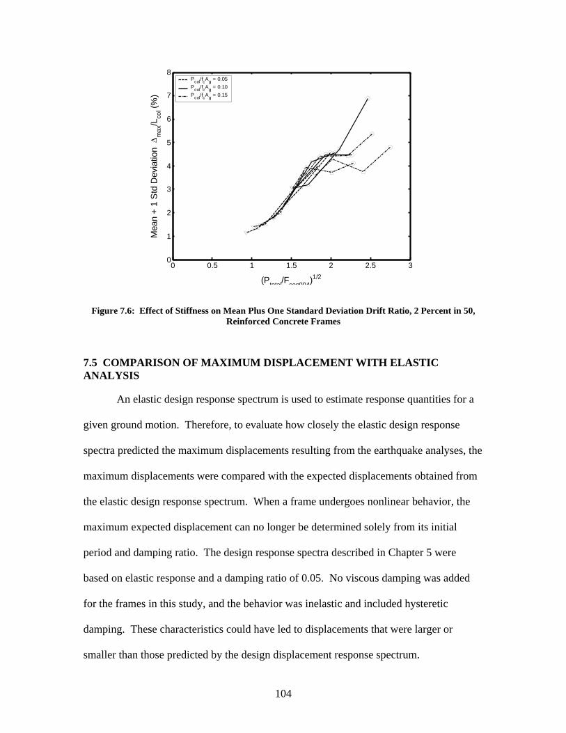
0 0.5 1 1.5 2 2.5 30
1
2
3
4
5
6
7
8
(Ptotal/Fcon004)1/2
Mea
n +
1 S
td D
evia
tion
Δm
ax/L
col (%
)
Pcol/fcAg = 0.05Pcol/fcAg = 0.10Pcol/fcAg = 0.15
Figure 7.6: Effect of Stiffness on Mean Plus One Standard Deviation Drift Ratio, 2 Percent in 50, Reinforced Concrete Frames
7.5 COMPARISON OF MAXIMUM DISPLACEMENT WITH ELASTIC ANALYSIS
An elastic design response spectrum is used to estimate response quantities for a
given ground motion. Therefore, to evaluate how closely the elastic design response
spectra predicted the maximum displacements resulting from the earthquake analyses, the
maximum displacements were compared with the expected displacements obtained from
the elastic design response spectrum. When a frame undergoes nonlinear behavior, the
maximum expected displacement can no longer be determined solely from its initial
period and damping ratio. The design response spectra described in Chapter 5 were
based on elastic response and a damping ratio of 0.05. No viscous damping was added
for the frames in this study, and the behavior was inelastic and included hysteretic
damping. These characteristics could have led to displacements that were larger or
smaller than those predicted by the design displacement response spectrum.
104
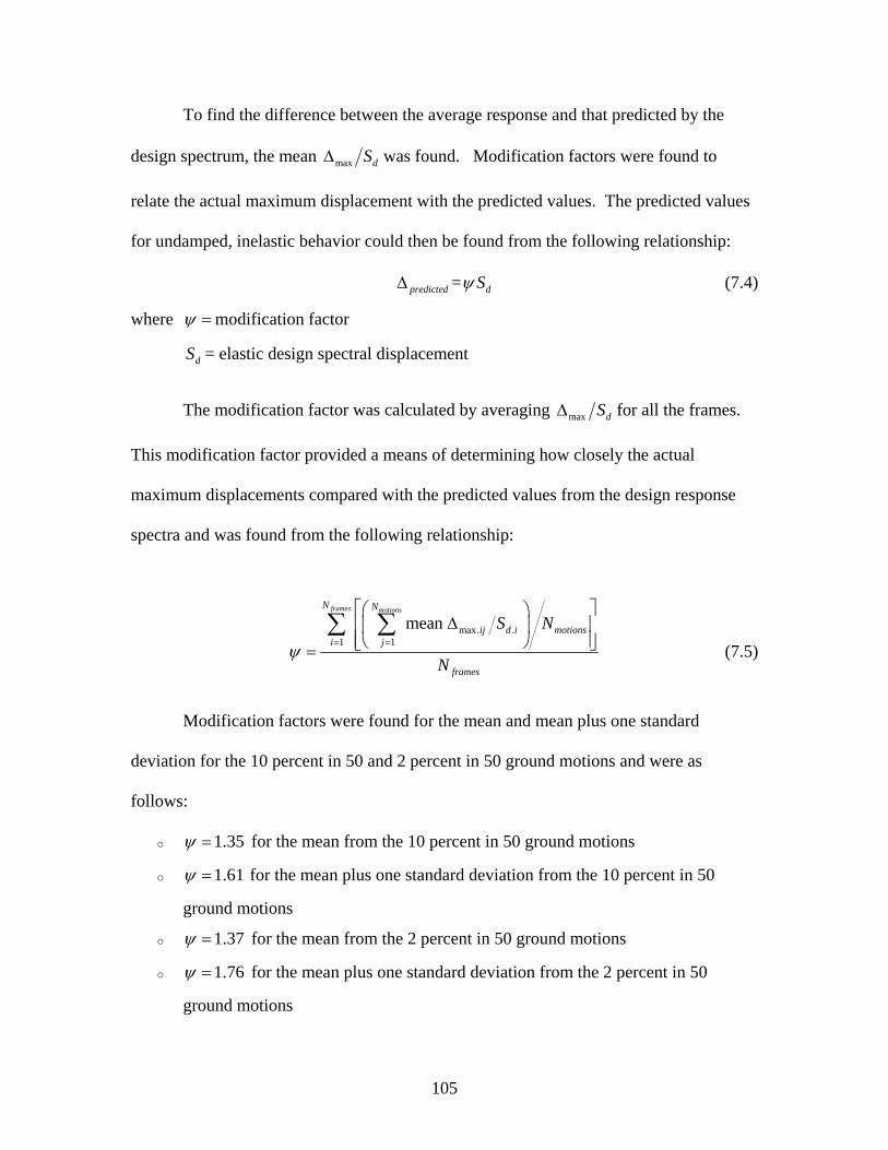
To find the difference between the average response and that predicted by the
design spectrum, the mean max dSΔ was found. Modification factors were found to
relate the actual maximum displacement with the predicted values. The predicted values
for undamped, inelastic behavior could then be found from the following relationship:
=predicted dSψΔ (7.4)
where ψ = modification factor
= elastic design spectral displacement dS
The modification factor was calculated by averaging max dSΔ for all the frames.
This modification factor provided a means of determining how closely the actual
maximum displacements compared with the predicted values from the design response
spectra and was found from the following relationship:
max. .
1 1mean
frames motionsN N
ij d i motionsi j
frames
S N
Nψ
= =
⎡ ⎤⎛ ⎞Δ⎢ ⎥⎜ ⎟
⎢⎝ ⎠⎣=∑ ∑
⎥⎦ (7.5)
Modification factors were found for the mean and mean plus one standard
deviation for the 10 percent in 50 and 2 percent in 50 ground motions and were as
follows:
o 1.35ψ = for the mean from the 10 percent in 50 ground motions
o 1.61ψ = for the mean plus one standard deviation from the 10 percent in 50
ground motions
o 1.37ψ = for the mean from the 2 percent in 50 ground motions
o 1.76ψ = for the mean plus one standard deviation from the 2 percent in 50
ground motions
105
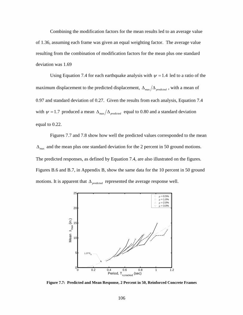
Combining the modification factors for the mean results led to an average value
of 1.36, assuming each frame was given an equal weighting factor. The average value
resulting from the combination of modification factors for the mean plus one standard
deviation was 1.69
Using Equation 7.4 for each earthquake analysis with 1.4ψ = led to a ratio of the
maximum displacement to the predicted displacement, max predictedΔ Δ , with a mean of
0.97 and standard deviation of 0.27. Given the results from each analysis, Equation 7.4
with 1.7ψ = produced a mean max predictedΔ Δ equal to 0.80 and a standard deviation
equal to 0.22.
Figures 7.7 and 7.8 show how well the predicted values corresponded to the mean
and the mean plus one standard deviation for the 2 percent in 50 ground motions.
The predicted responses, as defined by Equation 7.4, are also illustrated on the figures.
Figures B.6 and B.7, in Appendix B, show the same data for the 10 percent in 50 ground
motions. It is apparent that represented the average response well.
maxΔ
predictedΔ
0 0.2 0.4 0.6 0.8 1 1.20
5
10
15
20
25
Period, Tn,cracked (sec)
Mea
n Δ
max
(in.
)
ρ = 0.5%ρ = 1.0%ρ = 2.0%ρ = 3.0%
1.37*Sd
Figure 7.7: Predicted and Mean Response, 2 Percent in 50, Reinforced Concrete Frames
106
0 0.2 0.4 0.6 0.8 1 1.20
5
10
15
20
25
Period, Tn,cracked (sec)
Mea
n +
1 S
td D
evia
tion
Δm
ax (i
n.)
Pcol/fcAg = 0.05Pcol/fcAg = 0.10Pcol/fcAg = 0.15
1.76*Sd
Figure 7.8: Predicted and Mean Plus One Standard Deviation Response, 2 Percent in 50, Reinforced Concrete Frames
Possible reasons for the discrepancies between the values predicted by the design
displacement response spectrum and the values from the earthquake analyses, and
therefore the need for the modification factors, include the following:
• The design response spectrum was based on a viscous damping ratio, ξ , of 0.05,
whereas no viscous damping was included for the frames in this study. This
could partially account for the under-prediction of the displacements from the
design response spectrum.
• The design response spectrum was created for elastic systems, but the frames
encountered inelastic behavior during the earthquake analyses. This inelastic
behavior could account for actual displacements larger than those predicted by
the design response spectrum.
107
• A difference existed between the target design spectrum and the scaled response
spectrum for each individual ground motion. These differences are apparent in
the figures of Appendix B.
7.6 INCORPORATION OF STRENGTH IN PREDICTION OF MAXIMUM DISPLACEMENT
To demonstrate the effect that strength had on the maximum displacement
response, the mean max dSΔ was plotted against a normalized strength, 004con aF S m ,
where and were the spectral displacement and spectral acceleration predicted from
the smooth design spectra (Figure 7.9). The data shown in these plots suggested a
bilinear relationship between
dS aS
max dSΔ and 004con aF S m . Above a value of 004con aF S m
of about 0.04, max dSΔ was approximately constant, whereas below this value, a linear
relationship appeared appropriate. Therefore, the predicted values for undamped,
inelastic behavior could be calculated with the following relationship:
( ) 004
004
for
for d con a
predictedd co
X S F S m
S F n aS m
α η β η
β η
⎧⎡ ⎤− + ≤⎪⎣ ⎦Δ = ⎨>⎪⎩
(7.6)
where α = absolute value slope of the linear portion
η = value of 004con aF S m corresponding to the transition from a linear
relationship to a constant value. This value was taken as 0.04.
X = value of 004con aF S m
β = value for the constant portion
= spectral displacement dS
108
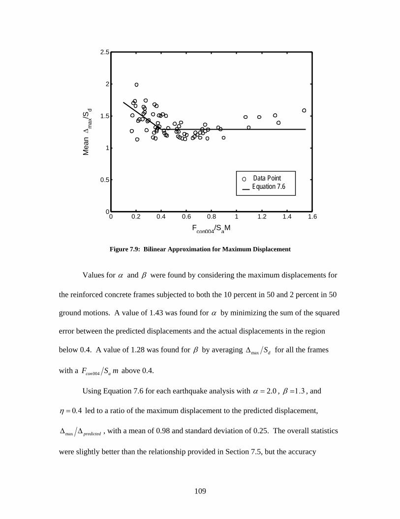
0 0.2 0.4 0.6 0.8 1 1.2 1.4 1.60
0.5
1
1.5
2
2.5
Fcon004/SaM
Mea
n Δ
max
/Sd
Data Point Equation 7.6
Figure 7.9: Bilinear Approximation for Maximum Displacement
Values for α and β were found by considering the maximum displacements for
the reinforced concrete frames subjected to both the 10 percent in 50 and 2 percent in 50
ground motions. A value of 1.43 was found for α by minimizing the sum of the squared
error between the predicted displacements and the actual displacements in the region
below 0.4. A value of 1.28 was found for β by averaging max dSΔ for all the frames
with a 004con aF S m above 0.4.
Using Equation 7.6 for each earthquake analysis with 2.0α = , β =1.3 , and
η = 0.4 led to a ratio of the maximum displacement to the predicted displacement,
max predictedΔ Δ , with a mean of 0.98 and standard deviation of 0.25. The overall statistics
were slightly better than the relationship provided in Section 7.5, but the accuracy
109
improved significantly for low values of the strength ratio. The predicted response
calculated from Equation 7.6 is shown in Figure 7.9.
7.7 TRENDS IN RESIDUAL DISPLACEMENT
A frame that has undergone significant yielding during a ground motion
excitation may not return to its original equilibrium position, resulting in a residual
displacement. The residual displacement can affect whether a structure needs to be
replaced after an earthquake or whether it can be repaired. If the residual displacements
do not require the structure to be replaced, they may still make repairing the structure
difficult. Therefore, residual displacements should be investigated independent of
maximum displacements (Kawashima et al. 1998).
For the 36 frames, residual displacements were calculated for each of the five 10
percent in 50 ground motions and the five 2 percent in 50 ground motions. The resulting
residual displacements from the 10 percent in 50 ground motions ranged from a
minimum of 0.0 in. (frame 5.005.10, ground motion 10-4, residual colLΔ = 0.00 percent) to
a maximum of 0.5 in. (frame 7.030.15, ground motion 10-3, residual colLΔ = 0.16 percent).
For the 2 percent in 50 ground motions, the residual displacements ranged from a
minimum of 0.0 in (frame 6.010.15, ground motion 2-4, residual colLΔ = 0.00 percent) to a
maximum of 2.9 in. (frame 7.030.10, ground motion 2-3, residual colLΔ = 0.86 percent).
Although the residual displacements resulting from ground motion 2-3 were
sizable, the resulting residual displacements on a whole were considerably smaller than
anticipated. The large weight used during this study may have contributed to the limited
residual displacements observed during this study. Field performance as well as
110
numerous research studies have suggested that reinforced concrete frames can experience
excessive residual displacements when subjected to a seismic event, whereas hybrid
frames experience significantly smaller residual displacements (Kawashima et al. 1998,
Zatar and Mutsuyoshi 2002, Sakai and Mahin 2004, and El-Sheikh et al. 1999). Because
the residual displacements were smaller than expected, especially when the results were
compared with the results of an elastic perfectly-plastic frame, a small-scale parametric
study was performed to determine the effects of the longitudinal mild steel’s strain-
hardening ratio and the viscous damping ratio on the residual displacements. The strain-
hardening ratio was defined as the ratio between the steel’s post-yielding tangent and its
initial elastic tangent. The strain-hardening ratio was varied during the parametric study
because Kawashima et al. (1998) suggested that the strain-hardening ratio has a
significant impact on residual drift.
Frame 7.020.05 was selected as the baseline frame for the parametric study
because it had one of the larger (but not the maximum) residual displacements ( =
0.8 in. and
residualΔ
residual colLΔ = 0.24 percent) resulting from the 2 percent in 50 ground motions.
Strain-hardening ratios of 0.001, 0.005, 0.009, 0.015, and 0.020 were selected for this
study. The value of 0.009 was selected because it was the strain-hardening ratio used
throughout the original parametric study. Viscous damping ratios of 0.00, 0.01, 0.02,
0.03, and 0.04 were selected to provide a range of practical values. The results of the
parametric study are summarized in Table 7.1, while Figure 7.10 presents the effect of
the strain-hardening ratio and viscous damping ratio on residual drift graphically.
111
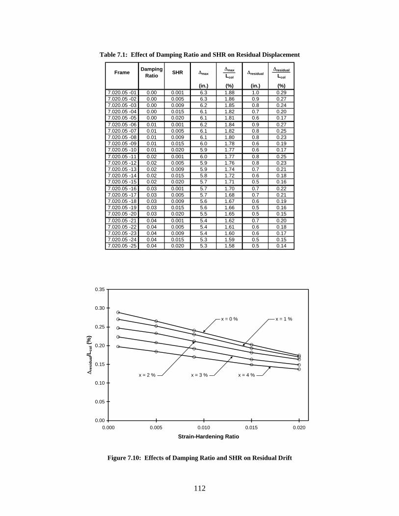
Table 7.1: Effect of Damping Ratio and SHR on Residual Displacement
(in.) (%) (in.) (%)7.020.05 -01 0.00 0.001 6.3 1.88 1.0 0.297.020.05 -02 0.00 0.005 6.3 1.86 0.9 0.277.020.05 -03 0.00 0.009 6.2 1.85 0.8 0.247.020.05 -04 0.00 0.015 6.1 1.82 0.7 0.207.020.05 -05 0.00 0.020 6.1 1.81 0.6 0.177.020.05 -06 0.01 0.001 6.2 1.84 0.9 0.277.020.05 -07 0.01 0.005 6.1 1.82 0.8 0.257.020.05 -08 0.01 0.009 6.1 1.80 0.8 0.237.020.05 -09 0.01 0.015 6.0 1.78 0.6 0.197.020.05 -10 0.01 0.020 5.9 1.77 0.6 0.177.020.05 -11 0.02 0.001 6.0 1.77 0.8 0.257.020.05 -12 0.02 0.005 5.9 1.76 0.8 0.237.020.05 -13 0.02 0.009 5.9 1.74 0.7 0.217.020.05 -14 0.02 0.015 5.8 1.72 0.6 0.187.020.05 -15 0.02 0.020 5.7 1.71 0.5 0.167.020.05 -16 0.03 0.001 5.7 1.70 0.7 0.227.020.05 -17 0.03 0.005 5.7 1.68 0.7 0.217.020.05 -18 0.03 0.009 5.6 1.67 0.6 0.197.020.05 -19 0.03 0.015 5.6 1.66 0.5 0.167.020.05 -20 0.03 0.020 5.5 1.65 0.5 0.157.020.05 -21 0.04 0.001 5.4 1.62 0.7 0.207.020.05 -22 0.04 0.005 5.4 1.61 0.6 0.187.020.05 -23 0.04 0.009 5.4 1.60 0.6 0.177.020.05 -24 0.04 0.015 5.3 1.59 0.5 0.157.020.05 -25 0.04 0.020 5.3 1.58 0.5 0.14
Δmax
LcolΔresidual
Δresidual
LcolFrame Damping
Ratio SHR Δmax
0.00
0.05
0.10
0.15
0.20
0.25
0.30
0.35
0.000 0.005 0.010 0.015 0.020
Strain-Hardening Ratio
Δre
sidu
al/L
col (
%)
x = 2 % x = 3 % x = 4 %
x = 0 % x = 1 %
Figure 7.10: Effects of Damping Ratio and SHR on Residual Drift
112
The results summarized in Table 7.1 and pictured in Figure 7.10 show that
varying the strain-hardening ratio from 0.001 to 0.020 resulted in a decrease in
residual colLΔ of 30 to 40 percent. As the damping ratio increased from 0 percent to 4
percent, a decrease in residual colLΔ of 20 to 30 percent was observed. These observations
indicate that the resulting residual displacements were significantly affected by the
assumptions made during the modeling of the frames. This conclusion suggests that a
detailed investigation is required to determine the effect of various parameters on residual
displacements. Experimental test results are needed to calibrate the analytic models to
accurately predict residual displacements. Therefore, complete residual displacement
results are not presented here.
The results summarized in Table 7.1 also indicate that maximum displacements
were not considerably affected by the strain-hardening ratio (3 percent variation between
values of 0.001 and 0.020) or viscous damping ratio (14 percent variation between values
of 0.00 and 0.04). This provides additional confidence in the maximum displacement
results presented in this document.
113
CHAPTER 8 PUSHOVER ANALYSES OF HYBRID FRAMES
This chapter focuses on the pushover analysis of the hybrid frames that were part
of the parametric study. The pushover analyses were conducted to determine first yield
properties, initial cracked properties, estimated nominal yield displacement, and
maximum strength of hybrid frames.
This chapter describes the parameters that were varied for the hybrid frames
(Section 8.1), key characteristics that were useful for comparison among pushover
analyses (Section 8.2), and key results obtained from these analyses (sections 8.3 through
8.5).
8.1 RANGE OF HYBRID PARAMETRIC STUDY
To evaluate the hybrid frame for a variety of configurations, the parameters to be
varied had to be selected. The parameters varied for the reinforced concrete frame study
alone were inadequate for the hybrid frame study because prestressing introduces
additional parameters. Therefore, parameters had to be selected that would account for
the factors introduced by the prestessing, such as combined moment capacity and re-
centering ability, while also providing a sensible link between the parameters selected for
the reinforced concrete frames and the hybrid frames. This section presents the rationale
for the parameters that were varied for the hybrid frames. The following four parameters
were selected to be varied during this study:
o column aspect ratio, col colL D
o axial-load ratio, '( )col c gP f A
o equivalent reinforcement ratio, ( )eq s y p py yf f fρ ρ ρ= +
114
o re-centering ratio, ( )0rc col p p s yP A f A fλ = + .
On the basis of the reasoning provided in Section 6.1, a column diameter, , of
48 in. was used for all hybrid frames. The results found during this study can be scaled to
provide estimates for frames with other column diameters. To provide a basis for
comparison between the reinforced concrete frames and the hybrid frames, parameters
similar to those used for the reinforced concrete frames were selected.
colD
The parameters selected for the reinforced concrete frames were all independent
from one another; therefore, every combination of parameters was used (Chapter 6). On
the other hand, the parameters selected for the hybrid frames were interdependent;
therefore, every combination of the parameters would not result in quantities that were
physically possible. For example, it is not possible to have a negative area of prestressing
steel. The following paragraphs provide a description of the parameters.
8.1.1 Column Aspect Ratio, col colL D
The column aspect ratio was defined as the clear height between the top of the
foundation and the bottom of the cap-beam divided by the diameter of the column,
col colL D . The required minimum vertical clearance from Article 1120.04 (5) of the
WSDOT Design Manual (WSDOT 2002b) is 16.5 ft. For the frames with 48-in.-diameter
columns, this resulted in a minimum col colL D of 4.125. This value was increased to 5, 6,
and 7 for the col colL D for this study.
8.1.2 Axial-Load Ratio, '( )col c gP f A
The axial-load ratio was defined as the compressive axial-load on a column
divided by the product of the unconfined concrete compressive strength and the gross
115
area of the column’s cross-section, '(col c gP f A ) . Article 5.10.11.4.1 b of the AASHTO
LRFD Bridge Design Specification (AASHTO 1998) permits axial-load ratios of up to
0.20. The prototype bridge described in Chapter 4 had a '(col c gP f A ) value of
approximately 0.075. To include a variety of values in the allowable range, axial-load
ratios of 0.05, 0.10, and 0.15 were selected for this study.
8.1.3 Equivalent Reinforcement Ratio
The equivalent reinforcement ratio was selected to account for the contribution of
both mild reinforcing steel and prestressing steel to the lateral load resisting capacity of
the pier. The equivalent reinforcement ratio was defined by Equation 8.1.
s y p peq
y
yf ff
ρ ρρ
+= (8.1)
where sρ = area of longitudinal mild steel divided by the gross cross-sectional area of
the column, s gA A
yf = yield strength of the longitudinal mild steel, taken as 60 ksi
pρ = area of prestressing steel divided by the gross cross-sectional area of the
column, p gA A
pyf = yield strength of the prestressing steel, taken as 243 ksi
Equivalent reinforcement ratios were chosen to represent hybrid frames with
strength similar to that of the reinforced concrete frames studied (chapters 6 and 7).
Accordingly, eqρ values of 0.005, 0.01, 0.02, and 0.03 were chosen for this study.
8.1.4 Re-centering Ratio, rcλ
The re-centering ratio was defined by Equation 8.2.
0col p prc
s y
P A fA f
λ+
= (8.2)
116
where = compressive axial-load on a column colP
= area of prestressing steel pA
0pf = stress in prestressing steel at zero drift
sA = area of longitudinal mild steel
yf = yield strength of longitudinal mild steel, taken as 60 ksi
The re-centering ratio was selected to estimate the ability of the frames to re-
center. It was assumed that the axial-load on the column, as well as the force from the
prestressing steel, would cause the frame to re-center if they were larger than the resisting
force from the longitudinal mild steel. For moderate to strong ground motions, re-
centering was expected to occur when the re-centering ratio was near 1.0. As the re-
centering ratio decreased below 1.0, the likelihood of re-centering was expected to
decrease. Re-centering was expected to occur for small earthquakes, regardless of the re-
centering ratio. Re-centering ratios of 0.0, 0.25, 0.50, 0.75, and 1.00 were chosen to
evaluate the re-centering ability of the frames.
8.1.5 Frame Designation
Frames were identified by the combination of their column aspect ratio,
equivalent reinforcement ratio, and re-centering ratio. For example, 5.020.050 was a
frame with 5col colL D = , 0.020eqρ = , and 0.50rcλ = ; 7.030.100 was a frame with
7col colL D = , 0.030eqρ = , and 1.00rcλ = . The axial-load ratio was not included in the
frame designation because the results were tabulated and plotted for individual values of
the axial-load ratio.
117
8.1.6 Practical Frame Combinations
The values presented in the previous paragraphs were target values. Instead of
creating frames from every combination of the four parameters, it was necessary to solve
for the variables in the parameters and use only the combinations that resulted in practical
frames. Many of the combinations resulted in a negative required prestressing area. This
is not physically possible, but the combinations represented frames that would most
likely re-center without prestressing steel. Only combinations of the parameters that
resulted in positive values of sA and were used for this study. The following method
was used to determine which of the combinations resulted in practical values.
pA
1. The yield strain of the prestressing steel was found from py py pf Eε = , where
pyf was the yield strength of the prestressing steel and was the modulus of
elasticity of the prestressing steel. From AASHTO Article 5.4.4,
pE
pyf was taken as
0.9 puf , where puf was the specified tensile strength of the prestressing steel and
was assumed to be 270 kips based on Article 6.1.3 from the WSDOT Bridge
Design Manual (WSDOT 2002a). was taken as 28,500 ksi (AASHTO 1998). pE
2. The stress in the prestressing steel at zero drift, 0pf , was found from the
following relationship:
pupcol
colcolpyp fE
LDL
f 7.0)(
0 ≤⎟⎟⎠
⎞⎜⎜⎝
⎛ Δ−= ε (8.3)
A maximum drift ratio, colLΔ , of 0.02 was assumed on the basis of the results of
the reinforced concrete frames subjected to 10 percent in 50 ground motions
(Chapter 7). The upper limit of 0.7 puf for 0pf was taken from AASHTO Article
118
5.9.3. This estimate was conservative because the lever arm was most likely
smaller than 2colD , which would result in a larger 0pf . For most of the frames,
the 0.7 puf limit controlled.
3. The required area of longitudinal mild steel was found by rearranging Equation
8.1 as follows:
eq y p pys g
y
f fA
fρ ρ⎛ ⎞−
= ⎜⎜⎝ ⎠
A⎟⎟ (8.4)
4. The required area of prestressing steel was then found from the re-center ratio as:
0
rc y colp
p
f PA
fλ −
= (8.5)
After the required area of longitudinal mild steel and prestressing steel was
calculated, combinations that resulted in a negative value for were omitted because
these combinations of parameters represented frames that were expected to re-center
without prestressing steel. The combinations that resulted in frames that were used for
this study are summarized in tables 8.1 and 8.2 for axial-load ratios equal to 0.05 and
0.10, respectively.
pA
119
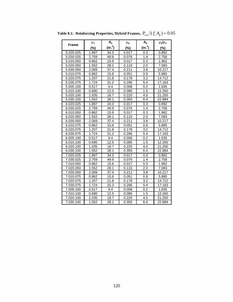
Table 8.1: Reinforcing Properties, Hybrid Frames, '( ) 0.05col c gP f A =
ρs As ρp Ap ρp/ρs
(%) (in.2) (%) (in.2) (%)5.020.025 1.897 34.3 0.017 0.3 0.8925.030.025 2.759 49.9 0.076 1.4 2.7585.010.050 0.862 15.6 0.017 0.3 1.9625.020.050 1.552 28.1 0.110 2.0 7.0835.030.050 2.069 37.4 0.211 3.8 10.2175.010.075 0.862 15.6 0.051 0.9 5.8855.020.075 1.207 21.8 0.178 3.2 14.7125.030.075 1.724 31.2 0.296 5.4 17.1635.005.100 0.517 9.4 0.008 0.2 1.6355.010.100 0.690 12.5 0.085 1.5 12.2605.020.100 1.035 18.7 0.220 4.0 21.2505.030.100 1.552 28.1 0.355 6.4 22.8846.020.025 1.897 34.3 0.017 0.3 0.8926.030.025 2.759 49.9 0.076 1.4 2.7586.010.050 0.862 15.6 0.017 0.3 1.9626.020.050 1.552 28.1 0.110 2.0 7.0836.030.050 2.069 37.4 0.211 3.8 10.2176.010.075 0.862 15.6 0.051 0.9 5.8856.020.075 1.207 21.8 0.178 3.2 14.7126.030.075 1.724 31.2 0.296 5.4 17.1636.005.100 0.517 9.4 0.008 0.2 1.6356.010.100 0.690 12.5 0.085 1.5 12.2606.020.100 1.035 18.7 0.220 4.0 21.2506.030.100 1.552 28.1 0.355 6.4 22.8847.020.025 1.897 34.3 0.017 0.3 0.8927.030.025 2.759 49.9 0.076 1.4 2.7587.010.050 0.862 15.6 0.017 0.3 1.9627.020.050 1.552 28.1 0.110 2.0 7.0837.030.050 2.069 37.4 0.211 3.8 10.2177.010.075 0.862 15.6 0.051 0.9 5.8857.020.075 1.207 21.8 0.178 3.2 14.7127.030.075 1.724 31.2 0.296 5.4 17.1637.005.100 0.517 9.4 0.008 0.2 1.6357.010.100 0.690 12.5 0.085 1.5 12.2607.020.100 1.035 18.7 0.220 4.0 21.2507.030.100 1.552 28.1 0.355 6.4 22.884
Frame
120
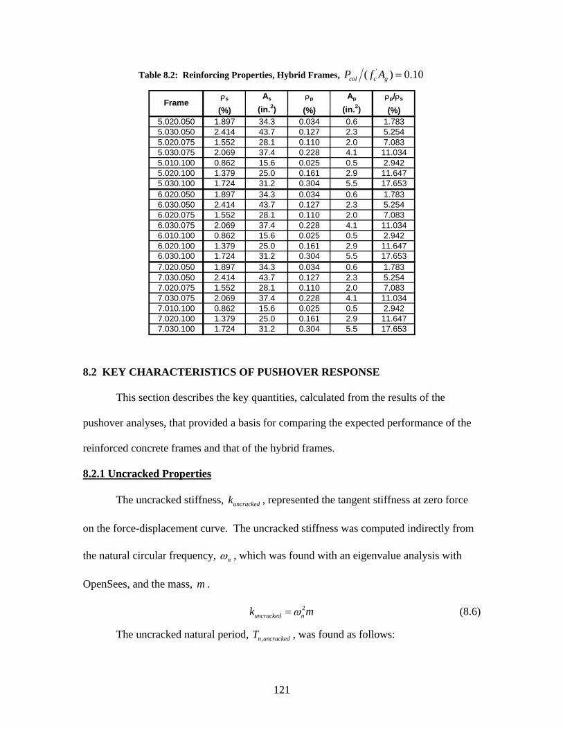
Table 8.2: Reinforcing Properties, Hybrid Frames, '( ) 0.10col c gP f A =
ρs As ρp Ap ρp/ρs
(%) (in.2) (%) (in.2) (%)5.020.050 1.897 34.3 0.034 0.6 1.7835.030.050 2.414 43.7 0.127 2.3 5.2545.020.075 1.552 28.1 0.110 2.0 7.0835.030.075 2.069 37.4 0.228 4.1 11.0345.010.100 0.862 15.6 0.025 0.5 2.9425.020.100 1.379 25.0 0.161 2.9 11.6475.030.100 1.724 31.2 0.304 5.5 17.6536.020.050 1.897 34.3 0.034 0.6 1.7836.030.050 2.414 43.7 0.127 2.3 5.2546.020.075 1.552 28.1 0.110 2.0 7.0836.030.075 2.069 37.4 0.228 4.1 11.0346.010.100 0.862 15.6 0.025 0.5 2.9426.020.100 1.379 25.0 0.161 2.9 11.6476.030.100 1.724 31.2 0.304 5.5 17.6537.020.050 1.897 34.3 0.034 0.6 1.7837.030.050 2.414 43.7 0.127 2.3 5.2547.020.075 1.552 28.1 0.110 2.0 7.0837.030.075 2.069 37.4 0.228 4.1 11.0347.010.100 0.862 15.6 0.025 0.5 2.9427.020.100 1.379 25.0 0.161 2.9 11.6477.030.100 1.724 31.2 0.304 5.5 17.653
Frame
8.2 KEY CHARACTERISTICS OF PUSHOVER RESPONSE
This section describes the key quantities, calculated from the results of the
pushover analyses, that provided a basis for comparing the expected performance of the
reinforced concrete frames and that of the hybrid frames.
8.2.1 Uncracked Properties
The uncracked stiffness, , represented the tangent stiffness at zero force
on the force-displacement curve. The uncracked stiffness was computed indirectly from
the natural circular frequency,
uncrackedk
nω , which was found with an eigenvalue analysis with
OpenSees, and the mass, . m
(8.6) 2uncracked nk ω= m
The uncracked natural period, , was found as follows: ,n uncrackedT
121
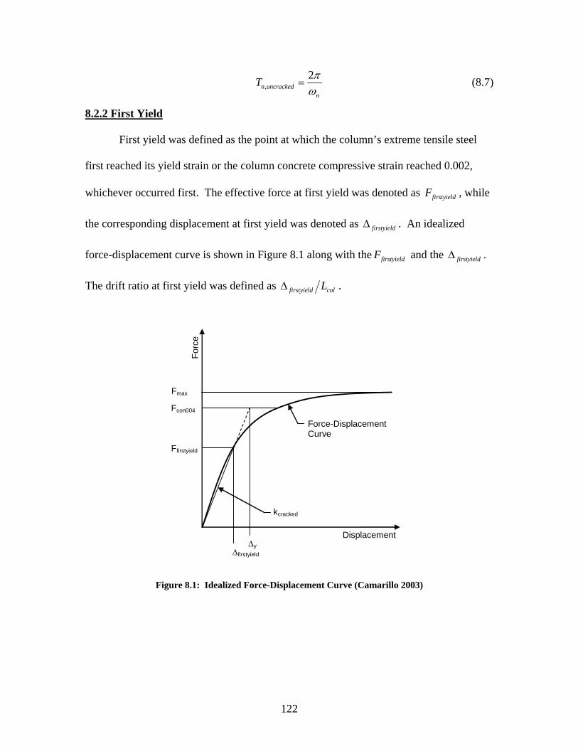
,2
n uncrackedn
T πω
= (8.7)
8.2.2 First Yield
First yield was defined as the point at which the column’s extreme tensile steel
first reached its yield strain or the column concrete compressive strain reached 0.002,
whichever occurred first. The effective force at first yield was denoted as firstyieldF , while
the corresponding displacement at first yield was denoted as firstyieldΔ . An idealized
force-displacement curve is shown in Figure 8.1 along with the firstyieldF and the firstyieldΔ .
The drift ratio at first yield was defined as firstyield colLΔ .
Fcon004
Ffirstyield
ΔyΔfirstyield
Force-Displacement Curve
kcracked
Forc
e
Displacement
Fmax
Figure 8.1: Idealized Force-Displacement Curve (Camarillo 2003)
122
8.2.3 Cracked Properties
The initial cracked stiffness, , was found from the secant stiffness through
first yield (Figure 8.1).
crackedk
firstyieldcracked
firstyield
Fk =
Δ (8.8)
The cracked natural period, , was found as: ,n crackedT
, 2n crackedcracked
mTk
π= (8.9)
8.2.4 Stiffness Ratio, cracked uncrackedk k
The stiffness ratio was defined as the cracked stiffness divided by the uncracked
stiffness. This ratio reflected the loss of stiffness due to cracking.
8.2.5 Effective Force at a Concrete Strain of 0.004, 004conF
The effective force on the force-displacement curve that corresponded to the
concrete compressive strain first reaching 0.004 was denoted as and is shown in
Figure 8.1. This value was used to calculate the nominal yield displacement.
004conF
8.2.6 Nominal Yield Displacement, yΔ
A nominal yield displacement, yΔ , had to be defined to calculate displacement
ductility (Chapter 10). The force-displacement curve would become nonlinear during the
pushover analysis, as is evident in the idealized force-displacement curve of Figure 8.1.
As suggested by Priestley et al. (1996), to estimate yΔ , the force-displacement curve
was idealized with an equivalent bilinear relationship by extrapolating up to
. The nominal yield displacement was found from the following relationship:
crackedk
004conF
123
004con firstyieldy
firstyield
FF
ΔΔ = (8.10)
8.2.7 Maximum Force, maxF
The largest lateral force achieved during the pushover analysis was denoted as
. maxF
8.3 TRENDS IN STIFFNESS RATIO
The stiffness ratios that were calculated from the pushover analyses of the hybrid
frames are discussed in this section. The results for frames with an axial-load ratio of
0.05 are summarized in Table 8.3, and the results for frames with an axial-load ratio of
0.10 are summarized in Table 8.4. The tables show that cracked uncrackedk k ranged from
0.29 to 0.56. Similarly, Priestley et al. (1996) found that cracked uncrackedk k ranged from
0.35 to 0.60 for typical circular reinforced concrete columns with longitudinal
reinforcement ratios of between 0.01 and 0.03, and axial load ratios of between 0.10 and
0.30. The slightly lower values may reflect the cracked interface between the column and
the foundation or cap-beam.
124
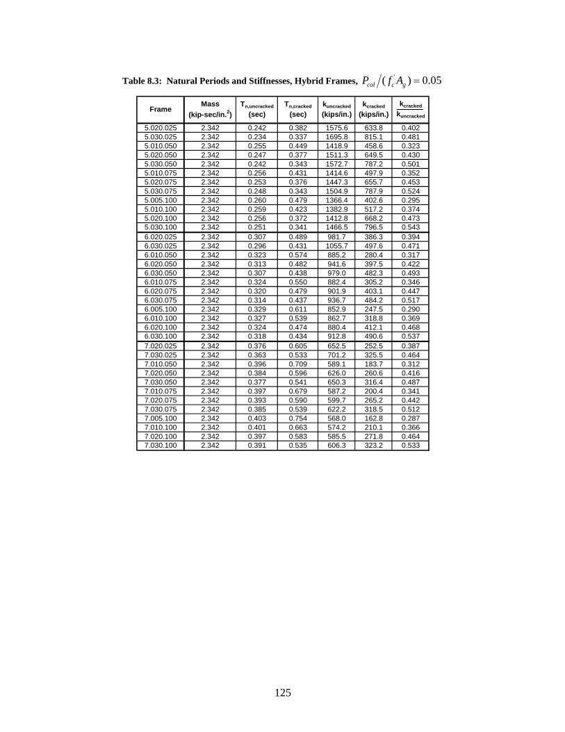
Table 8.3: Natural Periods and Stiffnesses, Hybrid Frames, '( ) 0.05col c gP f A =
5.020.025 2.342 0.242 0.382 1575.6 633.8 0.4025.030.025 2.342 0.234 0.337 1695.8 815.1 0.4815.010.050 2.342 0.255 0.449 1418.9 458.6 0.3235.020.050 2.342 0.247 0.377 1511.3 649.5 0.4305.030.050 2.342 0.242 0.343 1572.7 787.2 0.5015.010.075 2.342 0.256 0.431 1414.6 497.9 0.3525.020.075 2.342 0.253 0.376 1447.3 655.7 0.4535.030.075 2.342 0.248 0.343 1504.9 787.9 0.5245.005.100 2.342 0.260 0.479 1366.4 402.6 0.2955.010.100 2.342 0.259 0.423 1382.9 517.2 0.3745.020.100 2.342 0.256 0.372 1412.8 668.2 0.4735.030.100 2.342 0.251 0.341 1466.5 796.5 0.5436.020.025 2.342 0.307 0.489 981.7 386.3 0.3946.030.025 2.342 0.296 0.431 1055.7 497.6 0.4716.010.050 2.342 0.323 0.574 885.2 280.4 0.3176.020.050 2.342 0.313 0.482 941.6 397.5 0.4226.030.050 2.342 0.307 0.438 979.0 482.3 0.4936.010.075 2.342 0.324 0.550 882.4 305.2 0.3466.020.075 2.342 0.320 0.479 901.9 403.1 0.4476.030.075 2.342 0.314 0.437 936.7 484.2 0.5176.005.100 2.342 0.329 0.611 852.9 247.5 0.2906.010.100 2.342 0.327 0.539 862.7 318.8 0.3696.020.100 2.342 0.324 0.474 880.4 412.1 0.4686.030.100 2.342 0.318 0.434 912.8 490.6 0.5377.020.025 2.342 0.376 0.605 652.5 252.5 0.3877.030.025 2.342 0.363 0.533 701.2 325.5 0.4647.010.050 2.342 0.396 0.709 589.1 183.7 0.3127.020.050 2.342 0.384 0.596 626.0 260.6 0.4167.030.050 2.342 0.377 0.541 650.3 316.4 0.4877.010.075 2.342 0.397 0.679 587.2 200.4 0.3417.020.075 2.342 0.393 0.590 599.7 265.2 0.4427.030.075 2.342 0.385 0.539 622.2 318.5 0.5127.005.100 2.342 0.403 0.754 568.0 162.8 0.2877.010.100 2.342 0.401 0.663 574.2 210.1 0.3667.020.100 2.342 0.397 0.583 585.5 271.8 0.4647.030.100 2.342 0.391 0.535 606.3 323.2 0.533
kuncracked
(kips/in.)kcracked
(kips/in.)kcracked
kuncrackedFrame
Mass (kip-sec/in.2)
Tn,uncracked
(sec)Tn,cracked
(sec)
125
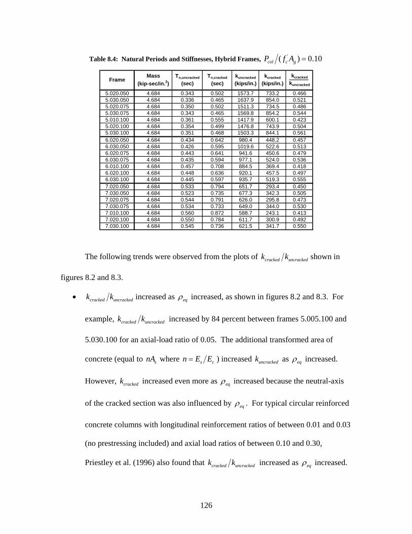
Table 8.4: Natural Periods and Stiffnesses, Hybrid Frames, '( ) 0.10col c gP f A =
5.020.050 4.684 0.343 0.502 1573.7 733.2 0.4665.030.050 4.684 0.336 0.465 1637.9 854.0 0.5215.020.075 4.684 0.350 0.502 1511.3 734.5 0.4865.030.075 4.684 0.343 0.465 1569.8 854.2 0.5445.010.100 4.684 0.361 0.555 1417.9 600.1 0.4235.020.100 4.684 0.354 0.499 1476.8 743.9 0.5045.030.100 4.684 0.351 0.468 1503.3 844.1 0.5616.020.050 4.684 0.434 0.642 980.4 448.2 0.4576.030.050 4.684 0.426 0.595 1019.6 522.6 0.5136.020.075 4.684 0.443 0.641 941.6 450.6 0.4796.030.075 4.684 0.435 0.594 977.1 524.0 0.5366.010.100 4.684 0.457 0.708 884.5 369.4 0.4186.020.100 4.684 0.448 0.636 920.1 457.5 0.4976.030.100 4.684 0.445 0.597 935.7 519.3 0.5557.020.050 4.684 0.533 0.794 651.7 293.4 0.4507.030.050 4.684 0.523 0.735 677.3 342.3 0.5057.020.075 4.684 0.544 0.791 626.0 295.8 0.4737.030.075 4.684 0.534 0.733 649.0 344.0 0.5307.010.100 4.684 0.560 0.872 588.7 243.1 0.4137.020.100 4.684 0.550 0.784 611.7 300.9 0.4927.030.100 4.684 0.545 0.736 621.5 341.7 0.550
kuncracked
(kips/in.)kcracked
(kips/in.)kcracked
kuncrackedFrame
Mass (kip-sec/in.2)
Tn,uncracked
(sec)Tn,cracked
(sec)
The following trends were observed from the plots of cracked uncrackedk k shown in
figures 8.2 and 8.3.
• cracked uncrackedk k increased as eqρ increased, as shown in figures 8.2 and 8.3. For
example, cracked uncrackedk k increased by 84 percent between frames 5.005.100 and
5.030.100 for an axial-load ratio of 0.05. The additional transformed area of
concrete (equal to snA where s cn E E= ) increased as uncrackedk eqρ increased.
However, increased even more as crackedk eqρ increased because the neutral-axis
of the cracked section was also influenced by eqρ . For typical circular reinforced
concrete columns with longitudinal reinforcement ratios of between 0.01 and 0.03
(no prestressing included) and axial load ratios of between 0.10 and 0.30,
Priestley et al. (1996) also found that cracked uncrackedk k increased as eqρ increased.
126
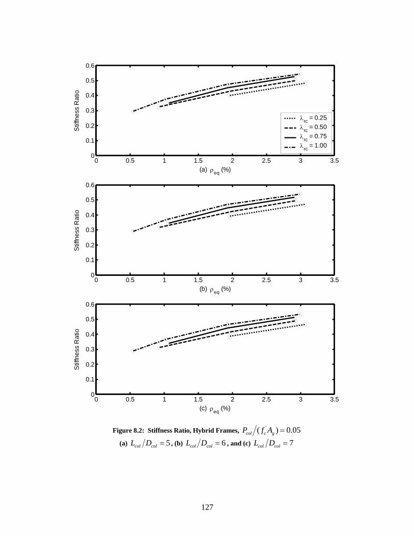
0 0.5 1 1.5 2 2.5 3 3.50
0.1
0.2
0.3
0.4
0.5
0.6
(a) ρeq (%)
Stif
fnes
s R
atio
λrc = 0.25λrc = 0.50λrc = 0.75λrc = 1.00
0 0.5 1 1.5 2 2.5 3 3.50
0.1
0.2
0.3
0.4
0.5
0.6
(b) ρeq (%)
Stif
fnes
s R
atio
0 0.5 1 1.5 2 2.5 3 3.50
0.1
0.2
0.3
0.4
0.5
0.6
(c) ρeq (%)
Stif
fnes
s R
atio
Figure 8.2: Stiffness Ratio, Hybrid Frames, '( ) 0.05col c gP f A =
(a) 5col colL D = , (b) 6col colL D = , and (c) 7col colL D =
127
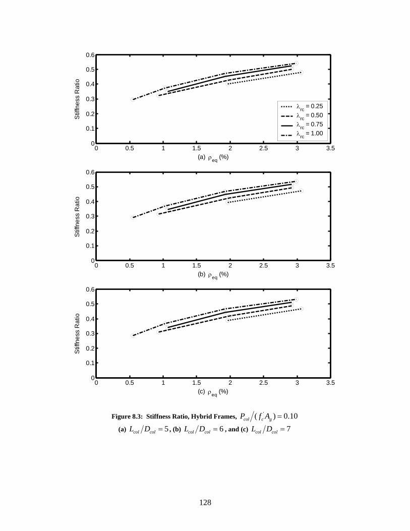
0 0.5 1 1.5 2 2.5 3 3.50
0.1
0.2
0.3
0.4
0.5
0.6
(a) ρeq (%)
Stif
fnes
s R
atio
λrc = 0.25λrc = 0.50λrc = 0.75λrc = 1.00
0 0.5 1 1.5 2 2.5 3 3.50
0.1
0.2
0.3
0.4
0.5
0.6
(b) ρeq (%)
Stif
fnes
s R
atio
0 0.5 1 1.5 2 2.5 3 3.50
0.1
0.2
0.3
0.4
0.5
0.6
(c) ρeq (%)
Stif
fnes
s R
atio
Figure 8.3: Stiffness Ratio, Hybrid Frames, '( ) 0.10col c gP f A =
(a) 5col colL D = , (b) 6col colL D = , and (c) 7col colL D =
128
• cracked uncrackedk k increased slightly as '(col c gP f A ) increased (figures 8.2 and 8.3).
The stiffness ratio increased by 13 percent for frame 5.010.100 as
'(col c gP f A ) increased from 0.05 to 0.10. was influenced bycrackedk '( )col c gP f A
because, as the axial-load ratio increased, the distance from the neutral-axis to the
extreme compression face of the column cross-section also increased, resulting in
an increased cracked stiffness. Paulay and Priestley (1992) presented values for
the cracked stiffness with larger values for larger axial-loads. Priestley et al.
(1996) also found that cracked uncrackedk k increased as '(col c gP f A ) increased.
• cracked uncrackedk k remained essentially unchanged as col colL D varied. This trend
indicated that and were equally influenced by crackedk uncrackedk col colL D . As
expected from the relationship for stiffness ( )3colk EI Lα= , both and
decreased as
uncrackedk
crackedk col colL D increased.
• From figures 8.2 and 8.3 it is evident that cracked uncrackedk k slightly increased as
rcλ increased. For example, cracked uncrackedk k increased by 18 percent for an axial-
load ratio of 0.05 between frames 5.020.025 to 5.020.100. This trend was
consistent with the trend observed for the axial-load ratio because as rcλ
increased, the additional prestressing increased the axial-load on the columns.
These trends indicate that eqρ had the greatest influence on cracked uncrackedk k ;
'(col c gP f A ) and rcλ had a small impact on cracked uncrackedk k ; and col colL D had almost no
effect on cracked uncrackedk k .
129
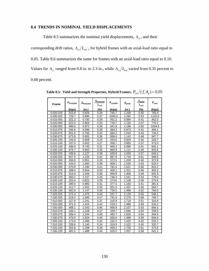
8.4 TRENDS IN NOMINAL YIELD DISPLACEMENTS
Table 8.5 summarizes the nominal yield displacements, yΔ , and their
corresponding drift ratios, y colLΔ , for hybrid frames with an axial-load ratio equal to
0.05. Table 8.6 summarizes the same for frames with an axial-load ratio equal to 0.10.
Values for ranged from 0.8 in. to 2.3 in., while yΔ y colLΔ varied from 0.35 percent to
0.68 percent.
Table 8.5: Yield and Strength Properties, Hybrid Frames, '( ) 0.05col c gP f A =
(kips) (in.) (%) (kips) (in.) (%) (kips)5.020.025 523.8 0.826 0.34 760.7 1.200 0.50 783.95.030.025 729.7 0.895 0.37 1045.0 1.282 0.53 1103.05.010.050 321.2 0.700 0.29 451.2 0.984 0.41 452.05.020.050 522.0 0.804 0.33 733.7 1.130 0.47 776.25.030.050 686.5 0.872 0.36 941.8 1.196 0.50 1004.55.010.075 346.6 0.696 0.29 484.2 0.973 0.41 494.15.020.075 501.5 0.765 0.32 684.2 1.044 0.43 726.35.030.075 673.8 0.855 0.36 899.6 1.142 0.48 947.75.005.100 244.8 0.608 0.25 333.6 0.829 0.35 333.75.010.100 337.5 0.652 0.27 456.7 0.883 0.37 475.05.020.100 496.5 0.743 0.31 665.3 0.996 0.41 692.15.030.100 676.7 0.850 0.35 884.9 1.111 0.46 926.66.020.025 435.6 1.127 0.39 630.8 1.633 0.57 645.26.030.025 607.0 1.220 0.42 867.8 1.744 0.61 908.56.010.050 266.8 0.951 0.33 372.5 1.328 0.46 372.86.020.050 434.0 1.092 0.38 608.1 1.530 0.53 633.46.030.050 570.8 1.184 0.41 781.6 1.621 0.56 824.26.010.075 288.0 0.944 0.33 400.1 1.311 0.46 402.26.020.075 416.9 1.034 0.36 566.8 1.406 0.49 591.56.030.075 560.2 1.157 0.40 746.4 1.541 0.54 778.06.005.100 203.4 0.822 0.29 274.6 1.109 0.39 274.66.010.100 280.5 0.880 0.31 377.0 1.183 0.41 381.66.020.100 412.7 1.002 0.35 551.0 1.337 0.46 564.76.030.100 562.6 1.147 0.40 734.0 1.496 0.52 760.57.020.025 372.4 1.475 0.44 537.7 2.129 0.63 546.17.030.025 519.2 1.595 0.47 741.0 2.276 0.68 769.77.010.050 227.9 1.241 0.37 315.9 1.719 0.51 316.67.020.050 371.0 1.424 0.42 518.2 1.989 0.59 532.27.030.050 488.1 1.543 0.46 666.8 2.107 0.63 694.37.010.075 246.1 1.228 0.37 339.7 1.695 0.50 339.97.020.075 356.4 1.344 0.40 482.7 1.820 0.54 494.57.030.075 479.0 1.504 0.45 636.6 1.999 0.59 656.07.005.100 173.6 1.066 0.32 232.0 1.425 0.42 232.17.010.100 239.6 1.140 0.34 319.9 1.522 0.45 320.77.020.100 352.8 1.298 0.39 469.2 1.726 0.51 473.57.030.100 481.0 1.488 0.44 626.0 1.937 0.58 641.2
Fcon004 ΔyieldΔyield
LcolFmaxFfirstyield Δfirstyield
Δfirstyield
LcolFrame
130
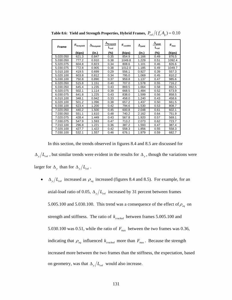
Table 8.6: Yield and Strength Properties, Hybrid Frames, '( ) 0.10col c gP f A =
(kips) (in.) (%) (kips) (in.) (%) (kips)5.020.050 621.3 0.847 0.35 854.9 1.166 0.49 876.55.030.050 777.2 0.910 0.38 1049.8 1.229 0.51 1092.45.020.075 604.8 0.823 0.34 808.6 1.101 0.46 826.65.030.075 772.8 0.905 0.38 1012.0 1.185 0.49 1049.75.010.100 419.5 0.699 0.29 556.1 0.927 0.39 557.35.020.100 603.8 0.812 0.34 795.0 1.069 0.45 810.25.030.100 750.8 0.890 0.37 959.8 1.137 0.47 985.66.020.050 515.8 1.151 0.40 707.0 1.578 0.55 716.26.030.050 645.4 1.235 0.43 869.5 1.664 0.58 892.56.020.075 502.1 1.114 0.39 668.5 1.484 0.52 673.96.030.075 641.8 1.225 0.43 838.0 1.599 0.56 858.56.010.100 348.1 0.942 0.33 458.0 1.240 0.43 458.66.020.100 501.2 1.096 0.38 657.2 1.437 0.50 661.56.030.100 623.4 1.200 0.42 794.6 1.530 0.53 808.77.020.050 440.2 1.500 0.45 600.8 2.048 0.61 602.17.030.050 551.1 1.610 0.48 740.2 2.162 0.64 751.97.020.075 428.4 1.449 0.43 567.8 1.920 0.57 569.17.030.075 547.9 1.593 0.47 713.2 2.073 0.62 723.77.010.100 296.8 1.221 0.36 387.2 1.593 0.47 387.47.020.100 427.7 1.422 0.42 558.3 1.856 0.55 558.37.030.100 532.1 1.557 0.46 676.1 1.979 0.59 682.7
Fcon004 ΔyieldΔyield
LcolFmaxFfirstyield Δfirstyield
Δfirstyield
LcolFrame
In this section, the trends observed in figures 8.4 and 8.5 are discussed for
y colLΔ , but similar trends were evident in the results for yΔ , though the variations were
larger for than for yΔ y colLΔ .
• y colLΔ increased as eqρ increased (figures 8.4 and 8.5). For example, for an
axial-load ratio of 0.05, y colLΔ increased by 31 percent between frames
5.005.100 and 5.030.100. This trend was a consequence of the effect of eqρ on
strength and stiffness. The ratio of between frames 5.005.100 and
5.030.100 was 0.51, while the ratio of between the two frames was 0.36,
indicating that
crackedk
maxF
eqρ influenced more than . Because the strength
increased more between the two frames than the stiffness, the expectation, based
on geometry, was that
crackedk maxF
y colLΔ would also increase.
131
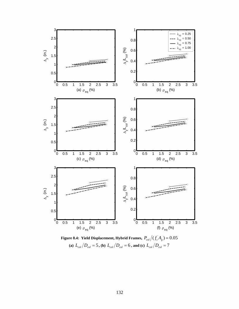
0 0.5 1 1.5 2 2.5 3 3.50
0.5
1
1.5
2
2.5
3
(a) ρeq (%)
Δy (
in.)
0 0.5 1 1.5 2 2.5 3 3.50
0.5
1
1.5
2
2.5
3
(c) ρeq (%)
Δy (
in.)
0 0.5 1 1.5 2 2.5 3 3.50
0.5
1
1.5
2
2.5
3
(e) ρeq (%)
Δy (
in.)
0 0.5 1 1.5 2 2.5 3 3.50
0.2
0.4
0.6
0.8
1
(b) ρeq (%)
Δy/L
col (%
)
λrc = 0.25λrc = 0.50λrc = 0.75λrc = 1.00
0 0.5 1 1.5 2 2.5 3 3.50
0.2
0.4
0.6
0.8
1
(d) ρeq (%)
Δy/L
col (%
)
0 0.5 1 1.5 2 2.5 3 3.50
0.2
0.4
0.6
0.8
1
(f) ρeq (%)
Δy/L
col (%
)
Figure 8.4: Yield Displacement, Hybrid Frames, '( ) 0.05col c gP f A =
(a) 5col colL D = , (b) 6col colL D = , and (c) 7col colL D =
132
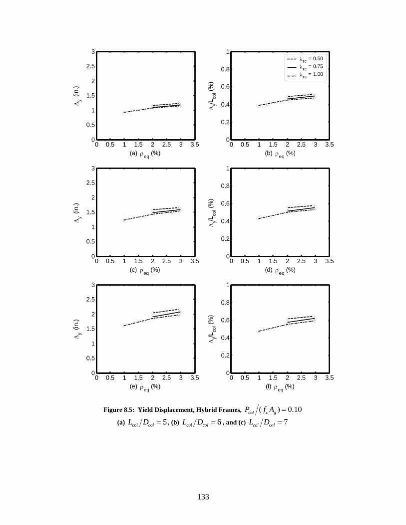
0 0.5 1 1.5 2 2.5 3 3.50
0.5
1
1.5
2
2.5
3
(a) ρeq (%)
Δy (
in.)
0 0.5 1 1.5 2 2.5 3 3.50
0.5
1
1.5
2
2.5
3
(c) ρeq (%)
Δy (
in.)
0 0.5 1 1.5 2 2.5 3 3.50
0.5
1
1.5
2
2.5
3
(e) ρeq (%)
Δy (
in.)
0 0.5 1 1.5 2 2.5 3 3.50
0.2
0.4
0.6
0.8
1
(b) ρeq (%)
Δy/L
col (%
)
λrc = 0.50λrc = 0.75λrc = 1.00
0 0.5 1 1.5 2 2.5 3 3.50
0.2
0.4
0.6
0.8
1
(d) ρeq (%)
Δy/L
col (%
)
0 0.5 1 1.5 2 2.5 3 3.50
0.2
0.4
0.6
0.8
1
(f) ρeq (%)
Δy/L
col (%
)
Figure 8.5: Yield Displacement, Hybrid Frames, '( ) 0.10col c gP f A =
(a) 5col colL D = , (b) 6col colL D = , and (c) 7col colL D =
133
• The first yield displacement also increased as eqρ increased (tables 8.5 and 8.6).
This trend can be demonstrated by evaluating the flexure of a reinforced concrete
square cross-section with a width equal to b . The depth of the neutral axis, , is
directly related to the quantity of steel in the cross-section and is given by
c
( ) ( )'g y cc A f f bρ= 0.85β where yf is the yield strength of the longitudinal mild
steel, 'cf is the concrete compressive strength, and β is the stress block depth
factor. From this relationship it is apparent that as the longitudinal steel ratio
increases, the depth of the neutral-axis also increases, resulting in an increase in
the displacement at first yield.
• From figures 8.4 and 8.5 it is clear that y colLΔ was essentially independent of
'(col c gP f A ) . No increase in y colLΔ was observed in these results because
'(col c gP f A ) affected the cracked stiffness as much as it affected the strength. For
example, the ratio of between frame 5.030.100 as the axial-load varied
from 0.05 to 0.10 was 0.94, and the ratio of was the same. Geometry dictates
that as the strength and the stiffness increase by the same amount,
crackedk
maxF
y colLΔ should
remain unchanged.
• y colLΔ increased as col colL D increased, as is evident in figures 8.4 and 8.5. For
example, y colLΔ increased by 26 percent between frames 5.030.100 and
7.030.100 for an axial-load ratio of 0.05. If the curvature at yield, yφ , is assumed
to be nearly constant and the yield displacement can be estimated as
2 6y y colLφΔ = , then an increase in col colL D would result in an increased y colLΔ .
134
• y colLΔ decreased as rcλ increased. The yield drift decreased by 13 percent
between frames 5.030.025 and 5.030.100 for an axial-load ratio of 0.05. The
results summarized in figures 8.4 and 8.5 suggest that as rcλ increased, both the
first yield displacement and yield displacement decreased. This can be explained
by the increase in the depth of the neutral-axis due to increased axial load as the
proportion of prestressing steel increased as rcλ increased.
In summary, eqρ had the greatest impact on y colLΔ ; col colL D and rcλ had a
moderate effect on y colLΔ ; and '(col c gP f A ) had almost no impact on y colLΔ .
8.5 TRENDS IN MAXIMUM FORCE
Tables 8.5 and 8.6 show that ranged from 232 to 1103 kips. The following
trends were observed from the results shown in figures 8.6 and 8.7.
maxF
• increased as maxF eqρ increased (figures 8.6 and 8.7). For example, the maximum
force increased 180 percent between frames 5.005.100 and 5.030.100 for an axial-
load ratio of 0.05. The flexural strength of a column is directly related to the
amount of longitudinal mild and prestressing steel provided in the cross-section.
Therefore, this trend corresponded to the increased flexural strength resulting
from the increased steel provided.
• increased as maxF '(col c gP f A ) increased (figures 8.6 and 8.7). An increase of 17
percent was observed for frame 5.010.100 as '(col c gP f A ) increased from 0.05 to
0.10. Because the axial-load ratios chosen for the hybrid frames were equal to or
below 0.10, the frames typically fell below the balanced failure point on their
135
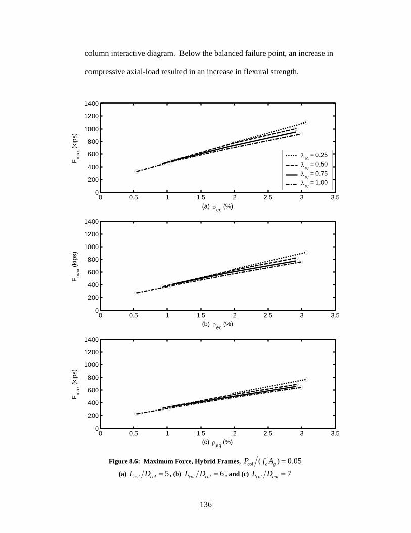
column interactive diagram. Below the balanced failure point, an increase in
compressive axial-load resulted in an increase in flexural strength.
0 0.5 1 1.5 2 2.5 3 3.50
200
400
600
800
1000
1200
1400
(a) ρeq (%)
F max
(kip
s)
λrc = 0.25λrc = 0.50λrc = 0.75λrc = 1.00
0 0.5 1 1.5 2 2.5 3 3.50
200
400
600
800
1000
1200
1400
(b) ρeq (%)
F max
(kip
s)
0 0.5 1 1.5 2 2.5 3 3.50
200
400
600
800
1000
1200
1400
(c) ρeq (%)
F max
(kip
s)
Figure 8.6: Maximum Force, Hybrid Frames, '( ) 0.05col c gP f A =
(a) 5col colL D = , (b) 6col colL D = , and (c) 7col colL D =
136
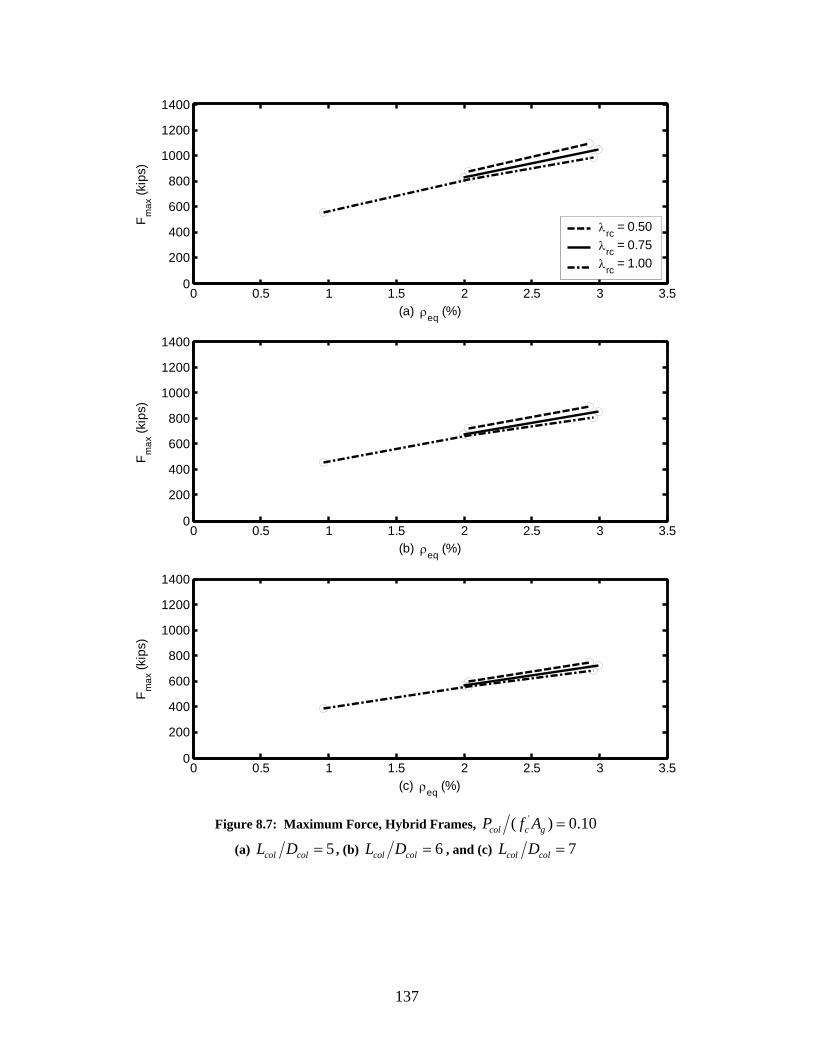
0 0.5 1 1.5 2 2.5 3 3.50
200
400
600
800
1000
1200
1400
(a) ρeq (%)
F max
(kip
s)
λrc = 0.50λrc = 0.75λrc = 1.00
0 0.5 1 1.5 2 2.5 3 3.50
200
400
600
800
1000
1200
1400
(b) ρeq (%)
F max
(kip
s)
0 0.5 1 1.5 2 2.5 3 3.50
200
400
600
800
1000
1200
1400
(c) ρeq (%)
F max
(kip
s)
Figure 8.7: Maximum Force, Hybrid Frames, '( ) 0.10col c gP f A =
(a) 5col colL D = , (b) 6col colL D = , and (c) 7col colL D =
137
• decreased as maxF col colL D increased. This trend may be observed in figures 8.6
and 8.7. For example, the maximum force decreased 31 percent between frames
5.030.100 and 7.030.100 for an axial-load ratio of 0.05. This decrease was caused
by the increased lever arm for the lateral load as col colL D increased.
• decreased as maxF rcλ increased, as is shown in figures 8.6 and 8.7. A decrease of
16 percent was observed between frames 5.030.025 and 5.030.100 for an axial-
load ratio of 0.05. This trend could be partially explained by the decreased
longitudinal mild steel provided as rcλ increased. Also, when the equivalent
reinforcement ratio was calculated, it was assumed in Equation 8.1 that the
prestressing steel had yielded. However, during the analyses the prestressing steel
did not yield.
On the basis of the results, eqρ had the greatest influence on ; maxF col colL D had a
moderate impact on ; and maxF '(col c gP f A ) and rcλ had the least impact on . maxF
138
CHAPTER 9 EARTHQUAKE ANALYSES OF HYBRID FRAMES
This chapter addresses the earthquake analyses of the hybrid frames performed in
the parametric study. The hybrid frames were subjected to the 10 ground motions
described in Chapter 5 to establish maximum displacements and residual displacements.
The 10 ground motions contained five motions with a 10 percent probability of
exceedance in 50 years (10 percent in 50) and five motions with a 2 percent probability of
exceedance in 50 years (2 percent in 50). This chapter describes the parameters that were
varied for the hybrid frames as part of the parametric study (Section 9.1), key quantities
used to evaluate frame performance (Section 9.2), and the results found during these
analyses (sections 9.3 through 9.7).
9.1 RANGE OF HYBRID PARAMETRIC STUDY
The parametric study considered variations of the baseline frame described in
Chapter 4. As described in Chapter 8, the following four parameters were varied for the
hybrid frames during the earthquake analyses:
o column aspect ratio, col colL D
o axial-load ratio, '( )col c gP f A
o equivalent reinforcement ratio, ( )eq s y p py yf f fρ ρ ρ= +
o re-centering ratio, ( )0rc col p p s yP A f A fλ = + .
9.2 KEY CHARACTERISTICS OF EARTHQUAKE RESPONSE
The same key quantities used to assess the performance of reinforced concrete
frames were used to provide insight into the expected performance of the hybrid frames.
These response quantities are presented in sections 9.3 through 9.7.
139
9.2.1 Maximum Displacement, maxΔ
The maximum displacement encountered in response to a given ground motion
was denoted as the maximum displacement, maxΔ . The maximum displacement was used
to calculate the displacement ductility demand as described in Chapter 10. Maximum
displacement was also used to provide insight into the likelihood that a given limit state
was exceeded (Chapter 10). The drift ratio corresponding to the maximum displacement
was defined as max colLΔ .
9.2.2 Residual Displacement, residualΔ
During the earthquake analysis of an inelastic frame, after yielding has occurred,
the frame may not vibrate about its original equilibrium position. Each time the frame
yields, the point about which the frame oscillates may shift. Therefore, after the ground
motion excitation has ended, the frame’s final position may not be the same as its initial
position, with the remaining displacement referred to as the residual displacement.
Residual displacement was defined as the difference between a frame’s position before
the ground motion excitation started (assumed to be 0.0 in.) and the frame’s position after
the ground motion excitation ended.
To estimate the residual displacement for this study, the free vibration of the
frame after the ground motion had stopped was considered. This was done because
viscous damping was not included in the frame analyses, and it would therefore take
significant time for the vibration to damp out completely. To estimate the residual
displacements, the maximum and minimum displacements over a time range starting 4
sec. after the ground excitation stopped, , 4set stop+ cΔ , and ending 9 sec. after the ground
140
excitation stopped, , were averaged. The residual displacements were
calculated from the following relationship:
, 9set stop+Δ c
, 4sec , 9sec , 4sec , 9semax( ) min( )2
t stop t stop t stop t stopresidual
+ + +Δ → Δ + Δ → ΔΔ = c+ (9.1)
9.3 TRENDS IN MAXIMUM DISPLACEMENT
This section reviews the maximum displacements encountered during the
earthquake analyses of the hybrid frames. Tables C.1 through C.4, found in Appendix C,
provide a complete summary of the results for the 10 percent in 50 ground motions and
the 2 percent in 50 ground motions for all the frames studied. The extreme values for the
maximum displacement resulting from the 10 percent in 50 ground motions were as
follows:
o Frames with axial-load ratio equal to 0.05
• Minimum: 0.9 in. (frame 5.010.075, ground motion 10-3,
max colLΔ = 0.38 percent)
• Maximum: 4.6 in. (frame 7.005.100, ground motion 10-5,
max colLΔ = 1.37 percent)
o Frames with axial-load ratio equal to 0.10
• Minimum: 0.9 in. (frame 5.030.075, ground motion 10-3,
max colLΔ = 0.38 percent)
• Maximum: 6.6 in. (frame 7.010.100, ground motion 10-1,
max colLΔ = 1.96 percent)
For the 2 percent in 50 ground motions, the maximum displacement ranged as
follows:
o Frames with axial-load ratio equal to 0.05
• Minimum: 1.7 in. (frame 5.030.025, ground motion 2-1,
max colLΔ = 0.72 percent)
141
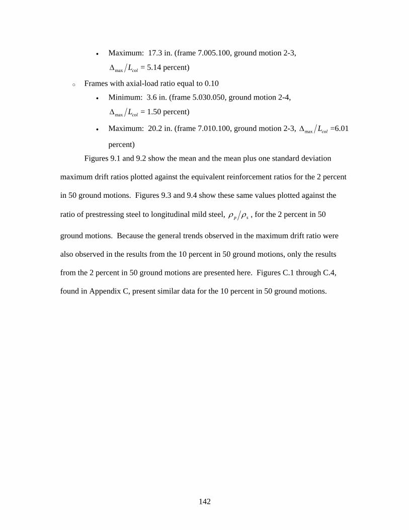
• Maximum: 17.3 in. (frame 7.005.100, ground motion 2-3,
max colLΔ = 5.14 percent)
o Frames with axial-load ratio equal to 0.10
• Minimum: 3.6 in. (frame 5.030.050, ground motion 2-4,
max colLΔ = 1.50 percent)
• Maximum: 20.2 in. (frame 7.010.100, ground motion 2-3, max colLΔ =6.01
percent)
Figures 9.1 and 9.2 show the mean and the mean plus one standard deviation
maximum drift ratios plotted against the equivalent reinforcement ratios for the 2 percent
in 50 ground motions. Figures 9.3 and 9.4 show these same values plotted against the
ratio of prestressing steel to longitudinal mild steel, p sρ ρ , for the 2 percent in 50
ground motions. Because the general trends observed in the maximum drift ratio were
also observed in the results from the 10 percent in 50 ground motions, only the results
from the 2 percent in 50 ground motions are presented here. Figures C.1 through C.4,
found in Appendix C, present similar data for the 10 percent in 50 ground motions.
142
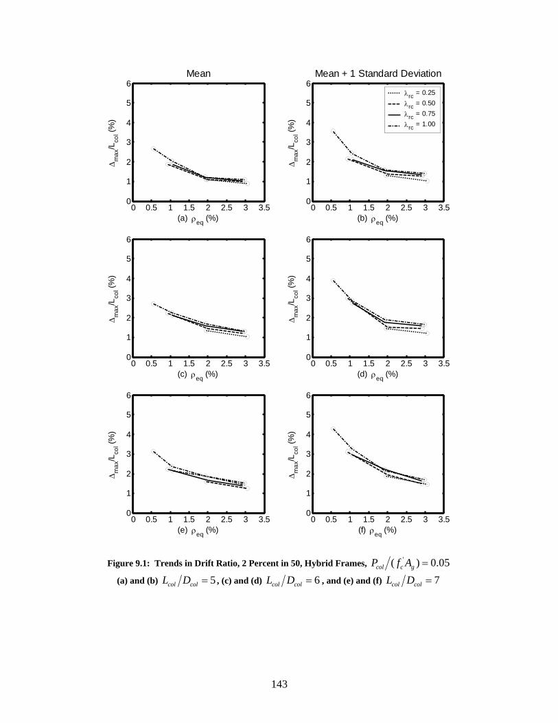
0 0.5 1 1.5 2 2.5 3 3.50
1
2
3
4
5
6
(a) ρeq (%)
Δm
ax/L
col (%
)
Mean
0 0.5 1 1.5 2 2.5 3 3.50
1
2
3
4
5
6
(c) ρeq (%)
Δm
ax/L
col (%
)
0 0.5 1 1.5 2 2.5 3 3.50
1
2
3
4
5
6
(e) ρeq (%)
Δm
ax/L
col (%
)
0 0.5 1 1.5 2 2.5 3 3.50
1
2
3
4
5
6
(b) ρeq (%)
Δm
ax/L
col (%
)
Mean + 1 Standard Deviation
λrc = 0.25λrc = 0.50λrc = 0.75λrc = 1.00
0 0.5 1 1.5 2 2.5 3 3.50
1
2
3
4
5
6
(d) ρeq (%)
Δm
ax/L
col (%
)
0 0.5 1 1.5 2 2.5 3 3.50
1
2
3
4
5
6
(f) ρeq (%)
Δm
ax/L
col (%
)
Figure 9.1: Trends in Drift Ratio, 2 Percent in 50, Hybrid Frames, '( ) 0.05col c gP f A =
(a) and (b) 5col colL D = , (c) and (d) 6col colL D = , and (e) and (f) 7col colL D =
143
0 0.5 1 1.5 2 2.5 3 3.50
1
2
3
4
5
6
(a) ρeq (%)
Δm
ax/L
col (%
)
Mean
0 0.5 1 1.5 2 2.5 3 3.50
1
2
3
4
5
6
(c) ρeq (%)
Δm
ax/L
col (%
)
0 0.5 1 1.5 2 2.5 3 3.50
1
2
3
4
5
6
(e) ρeq (%)
Δm
ax/L
col (%
)
0 0.5 1 1.5 2 2.5 3 3.50
1
2
3
4
5
6
(b) ρeq (%)
Δm
ax/L
col (%
)
Mean + 1 Standard Deviation
λrc = 0.50λrc = 0.75λrc = 1.00
0 0.5 1 1.5 2 2.5 3 3.50
1
2
3
4
5
6
(d) ρeq (%)
Δm
ax/L
col (%
)
0 0.5 1 1.5 2 2.5 3 3.50
1
2
3
4
5
6
(f) ρeq (%)
Δm
ax/L
col (%
)
Figure 9.2: Trends in Drift Ratio, 2 Percent in 50, Hybrid Frames, '( ) 0.10col c gP f A =
(a) and (b) 5col colL D = , (c) and (d) 6col colL D = , and (e) and (f) 7col colL D =
144
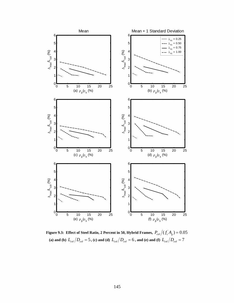
0 5 10 15 20 250
1
2
3
4
5
6
(a) ρp/ρs (%)
Δm
ax/L
col (%
)
Mean
0 5 10 15 20 250
1
2
3
4
5
6
(c) ρp/ρs (%)
Δm
ax/L
col (%
)
0 5 10 15 20 250
1
2
3
4
5
6
(e) ρp/ρs (%)
Δm
ax/L
col (%
)
0 5 10 15 20 250
1
2
3
4
5
6
(b) ρp/ρs (%)
Δm
ax/L
col (%
)
Mean + 1 Standard Deviation
λrc = 0.25λrc = 0.50λrc = 0.75λrc = 1.00
0 5 10 15 20 250
1
2
3
4
5
6
(d) ρp/ρs (%)
Δm
ax/L
col (%
)
0 5 10 15 20 250
1
2
3
4
5
6
(f) ρp/ρs (%)
Δm
ax/L
col (%
)
Figure 9.3: Effect of Steel Ratio, 2 Percent in 50, Hybrid Frames, '( ) 0.05col c gP f A =
(a) and (b) 5col colL D = , (c) and (d) 6col colL D = , and (e) and (f) 7col colL D =
145
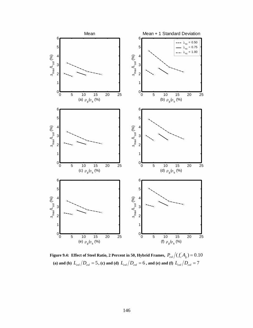
0 5 10 15 20 250
1
2
3
4
5
6
(a) ρp/ρs (%)
Δm
ax/L
col (%
)
Mean
0 5 10 15 20 250
1
2
3
4
5
6
(c) ρp/ρs (%)
Δm
ax/L
col (%
)
0 5 10 15 20 250
1
2
3
4
5
6
(e) ρp/ρs (%)
Δm
ax/L
col (%
)
0 5 10 15 20 250
1
2
3
4
5
6
(b) ρp/ρs (%)
Δm
ax/L
col (%
)
Mean + 1 Standard Deviation
λrc = 0.50λrc = 0.75λrc = 1.00
0 5 10 15 20 250
1
2
3
4
5
6
(d) ρp/ρs (%)
Δm
ax/L
col (%
)
0 5 10 15 20 250
1
2
3
4
5
6
(f) ρp/ρs (%)
Δm
ax/L
col (%
)
Figure 9.4: Effect of Steel Ratio, 2 Percent in 50, Hybrid Frames, '( ) 0.10col c gP f A =
(a) and (b) 5col colL D = , (c) and (d) 6col colL D = , and (e) and (f) 7col colL D =
146
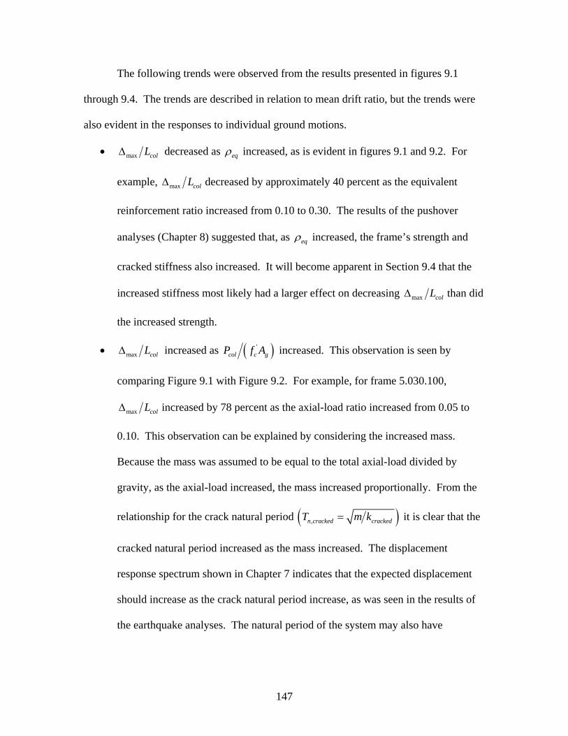
The following trends were observed from the results presented in figures 9.1
through 9.4. The trends are described in relation to mean drift ratio, but the trends were
also evident in the responses to individual ground motions.
• max colLΔ decreased as eqρ increased, as is evident in figures 9.1 and 9.2. For
example, max colLΔ decreased by approximately 40 percent as the equivalent
reinforcement ratio increased from 0.10 to 0.30. The results of the pushover
analyses (Chapter 8) suggested that, as eqρ increased, the frame’s strength and
cracked stiffness also increased. It will become apparent in Section 9.4 that the
increased stiffness most likely had a larger effect on decreasing max colLΔ than did
the increased strength.
• max colLΔ increased as ( )'col c gP f A increased. This observation is seen by
comparing Figure 9.1 with Figure 9.2. For example, for frame 5.030.100,
max colLΔ increased by 78 percent as the axial-load ratio increased from 0.05 to
0.10. This observation can be explained by considering the increased mass.
Because the mass was assumed to be equal to the total axial-load divided by
gravity, as the axial-load increased, the mass increased proportionally. From the
relationship for the crack natural period ( ),n cracked crackedT m k= it is clear that the
cracked natural period increased as the mass increased. The displacement
response spectrum shown in Chapter 7 indicates that the expected displacement
should increase as the crack natural period increase, as was seen in the results of
the earthquake analyses. The natural period of the system may also have
147
increased further because the stiffness may have been reduced as a result of the
effects. P − Δ
• max colLΔ increased as col colL D increased. This trend is reflected in Figure 9.2.
An increase of approximately 30 percent was observed in max colLΔ between
frames 5.030.100 and 7.030.100 for an axial-load ratio of 0.10. The relationship
between stiffness and column length ( )3col colk EI Lα= indicates that as the
column length increased, the frame’s stiffness decreased. This corresponded to
the results of the pushover analyses of the hybrid frames (Chapter 8). As
explained in the previous paragraph, as the stiffness decreased, the cracked
natural period increased, resulting in the larger max colLΔ .
• max colLΔ was almost independent of the rcλ , as is clear from figures 9.1 and 9.2.
For example, between frames 5.030.050 and 5.030.100, max colLΔ increased by
less that 10 percent. The pushover analyses of the hybrid frames showed that the
cracked stiffness remained effectively unchanged as the re-centering ratio
increased, and the maximum strength decreased slightly (approximately 15
percent) as the re-centering ratio increased. This trend suggests that the decreased
maximum strength contributed to the increased max colLΔ . Figures 9.3 and 9.4
reveal that for a given p sρ ρ , larger displacements will result from larger re-
centering ratios. This can be explained by noting that for a given p sρ ρ , a frame
with a larger re-centering ratio will have less mild longitudinal reinforcement
steel than a frame with a smaller re-centering ratio. The results of the pushover
analyses of the reinforced concrete frames (Chapter 6) showed that as the
148
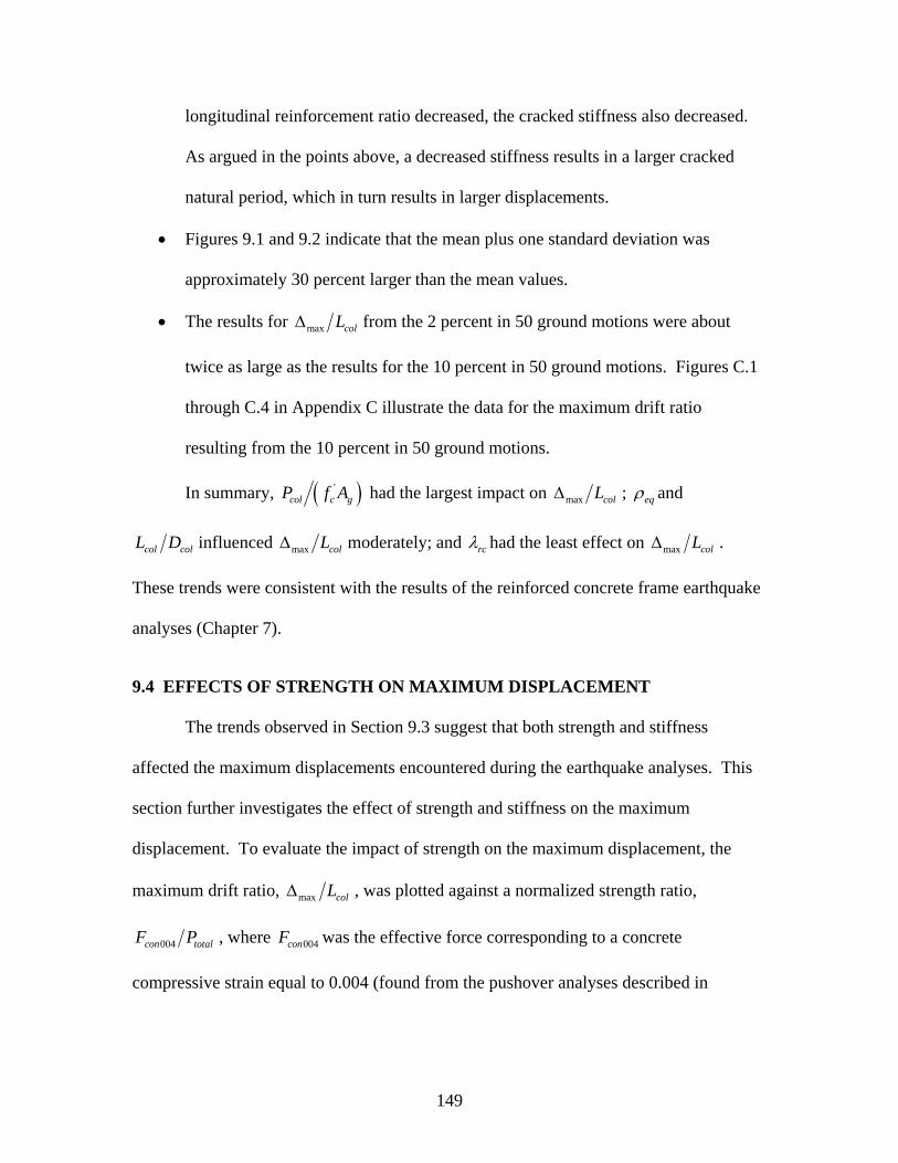
longitudinal reinforcement ratio decreased, the cracked stiffness also decreased.
As argued in the points above, a decreased stiffness results in a larger cracked
natural period, which in turn results in larger displacements.
• Figures 9.1 and 9.2 indicate that the mean plus one standard deviation was
approximately 30 percent larger than the mean values.
• The results for max colLΔ from the 2 percent in 50 ground motions were about
twice as large as the results for the 10 percent in 50 ground motions. Figures C.1
through C.4 in Appendix C illustrate the data for the maximum drift ratio
resulting from the 10 percent in 50 ground motions.
In summary, ( )'col c gP f A had the largest impact on max colLΔ ; eqρ and
col colL D influenced max colLΔ moderately; and rcλ had the least effect on max colLΔ .
These trends were consistent with the results of the reinforced concrete frame earthquake
analyses (Chapter 7).
9.4 EFFECTS OF STRENGTH ON MAXIMUM DISPLACEMENT
The trends observed in Section 9.3 suggest that both strength and stiffness
affected the maximum displacements encountered during the earthquake analyses. This
section further investigates the effect of strength and stiffness on the maximum
displacement. To evaluate the impact of strength on the maximum displacement, the
maximum drift ratio, max colLΔ , was plotted against a normalized strength ratio,
004con totalF P , where was the effective force corresponding to a concrete
compressive strain equal to 0.004 (found from the pushover analyses described in
004conF
149
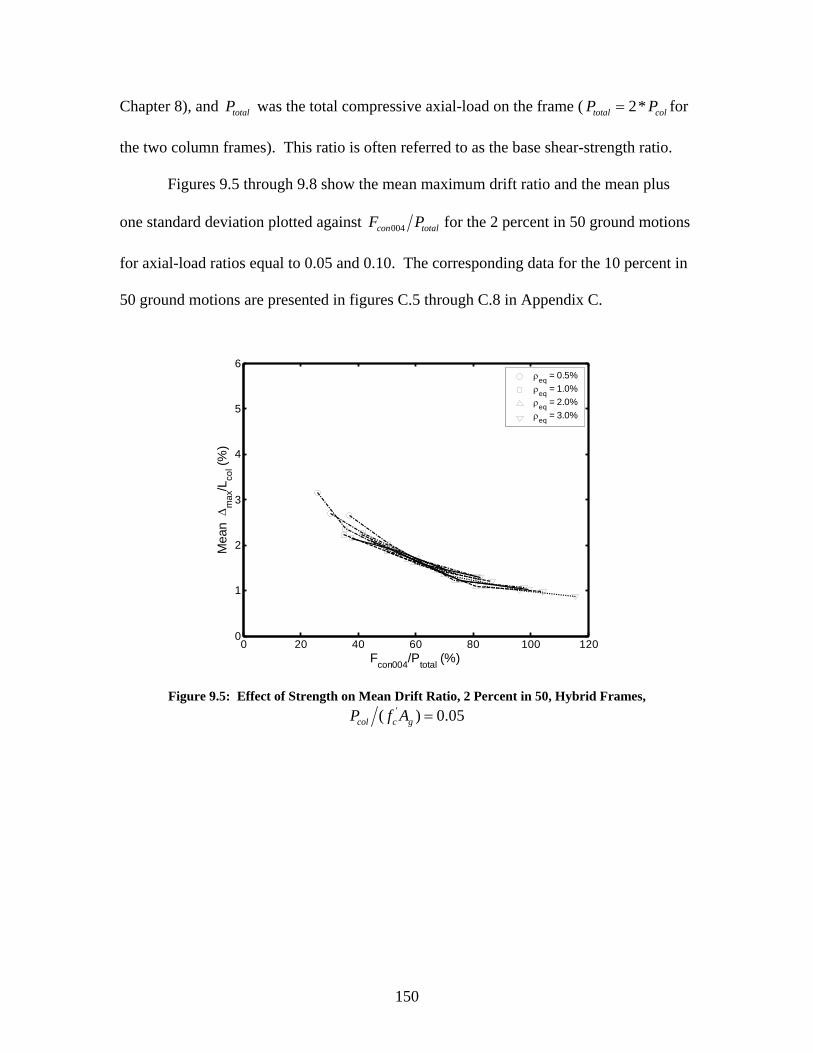
Chapter 8), and was the total compressive axial-load on the frame ( for
the two column frames). This ratio is often referred to as the base shear-strength ratio.
totalP 2*total colP P=
Figures 9.5 through 9.8 show the mean maximum drift ratio and the mean plus
one standard deviation plotted against 004con totalF P for the 2 percent in 50 ground motions
for axial-load ratios equal to 0.05 and 0.10. The corresponding data for the 10 percent in
50 ground motions are presented in figures C.5 through C.8 in Appendix C.
0 20 40 60 80 100 1200
1
2
3
4
5
6
Fcon004/Ptotal (%)
Mea
n Δ
max
/Lco
l (%)
ρeq = 0.5%ρeq = 1.0%ρeq = 2.0%ρeq = 3.0%
Figure 9.5: Effect of Strength on Mean Drift Ratio, 2 Percent in 50, Hybrid Frames,
'( ) 0.05col c gP f A =
150
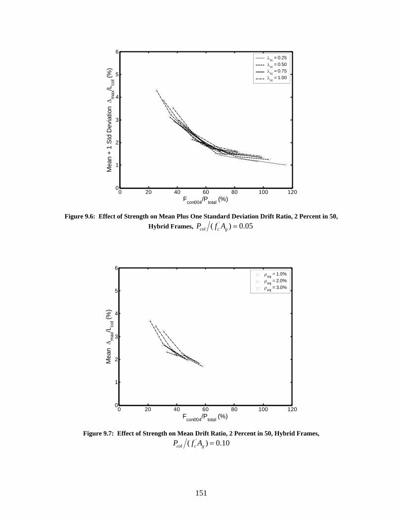
0 20 40 60 80 100 1200
1
2
3
4
5
6
Fcon004/Ptotal (%)
Mea
n +
1 S
td D
evia
tion
Δm
ax/L
col (%
)
λrc = 0.25λrc = 0.50λrc = 0.75λrc = 1.00
Figure 9.6: Effect of Strength on Mean Plus One Standard Deviation Drift Ratio, 2 Percent in 50,
Hybrid Frames, '( ) 0.05col c gP f A =
0 20 40 60 80 100 1200
1
2
3
4
5
6
Fcon004/Ptotal (%)
Mea
n Δ
max
/Lco
l (%)
ρeq = 1.0%ρeq = 2.0%ρeq = 3.0%
Figure 9.7: Effect of Strength on Mean Drift Ratio, 2 Percent in 50, Hybrid Frames,
'( ) 0.10col c gP f A =
151
0 20 40 60 80 100 1200
1
2
3
4
5
6
Fcon004/Ptotal (%)
Mea
n +
1 S
td D
evia
tion
Δm
ax/L
col (%
)
λrc = 0.50λrc = 0.75λrc = 1.00
Figure 9.8: Effect of Strength on Mean Plus One Standard Deviation Drift Ratio, 2 Percent in 50,
Hybrid Frames, '( ) 0.10col c gP f A =
The results shown in figures 9.5 through 9.8 fell onto relatively smooth curves.
The following observations were noted from the plots:
• max colLΔ decreased as 004con totalF P increased, suggesting that the maximum drift
ratio was at least partially affected by strength.
• The relationship between 004con totalF P and max colLΔ was nonlinear.
The strength ratio can also be an indirect indicator of stiffness. Priestley and
Paulay (2002) suggested that strength and stiffness are essentially proportional .
For this study, the mass on each frame was equal to the total axial-load divided by
gravity, . From these two relationships, the natural period can be expressed as:
( )k Fα=
g
totaln
P gTFα
= (9.2)
152
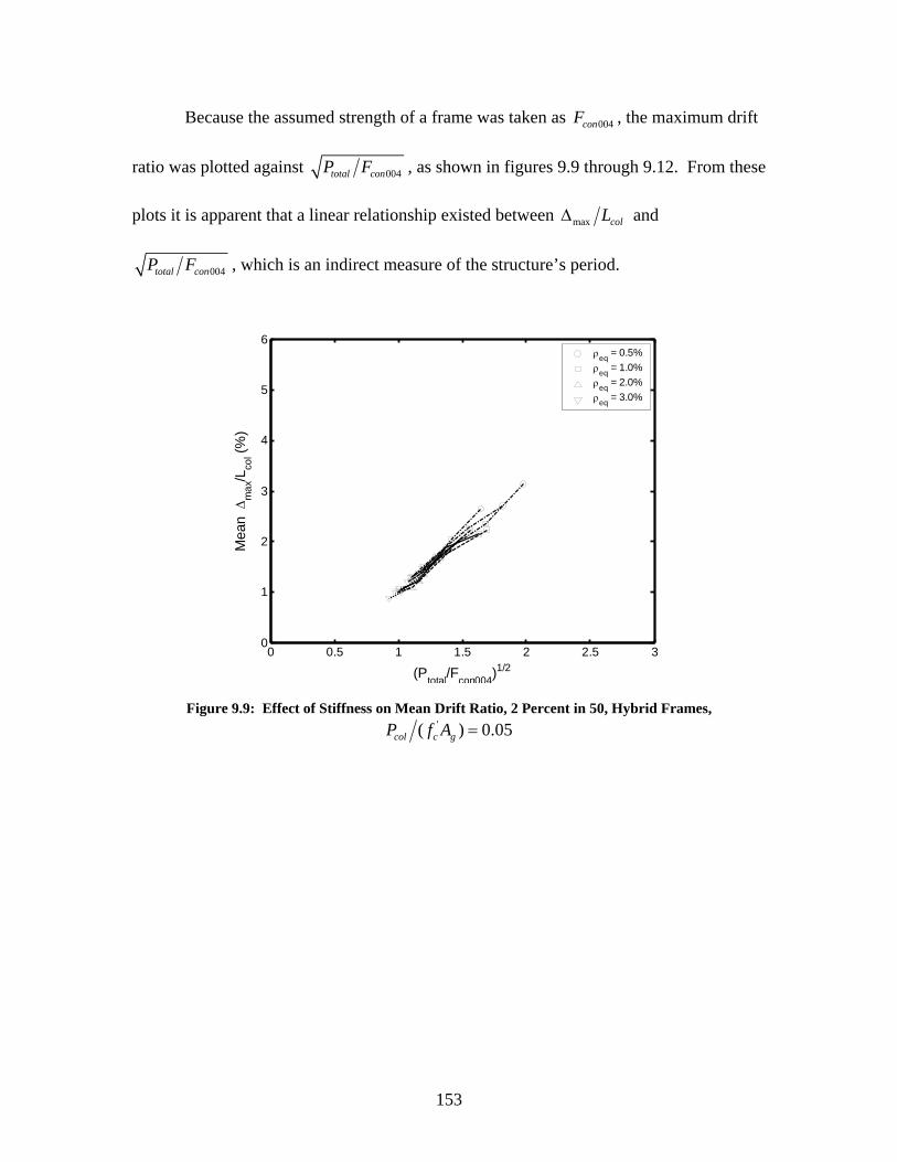
Because the assumed strength of a frame was taken as , the maximum drift
ratio was plotted against
004conF
004total conP F , as shown in figures 9.9 through 9.12. From these
plots it is apparent that a linear relationship existed between max colLΔ and
004total conP F , which is an indirect measure of the structure’s period.
0 0.5 1 1.5 2 2.5 30
1
2
3
4
5
6
(Ptotal/Fcon004)1/2
Mea
n Δ
max
/Lco
l (%)
ρeq = 0.5%ρeq = 1.0%ρeq = 2.0%ρeq = 3.0%
Figure 9.9: Effect of Stiffness on Mean Drift Ratio, 2 Percent in 50, Hybrid Frames,
'( ) 0.05col c gP f A =
153
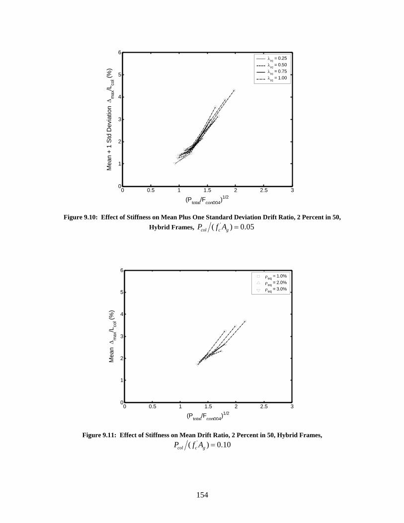
0 0.5 1 1.5 2 2.5 30
1
2
3
4
5
6
(Ptotal/Fcon004)1/2
Mea
n +
1 S
td D
evia
tion
Δm
ax/L
col (%
)
λrc = 0.25λrc = 0.50λrc = 0.75λrc = 1.00
Figure 9.10: Effect of Stiffness on Mean Plus One Standard Deviation Drift Ratio, 2 Percent in 50,
Hybrid Frames, '( ) 0.05col c gP f A =
0 0.5 1 1.5 2 2.5 30
1
2
3
4
5
6
(Ptotal/Fcon004)1/2
Mea
n Δ
max
/Lco
l (%)
ρeq = 1.0%ρeq = 2.0%ρeq = 3.0%
Figure 9.11: Effect of Stiffness on Mean Drift Ratio, 2 Percent in 50, Hybrid Frames,
'( ) 0.10col c gP f A =
154
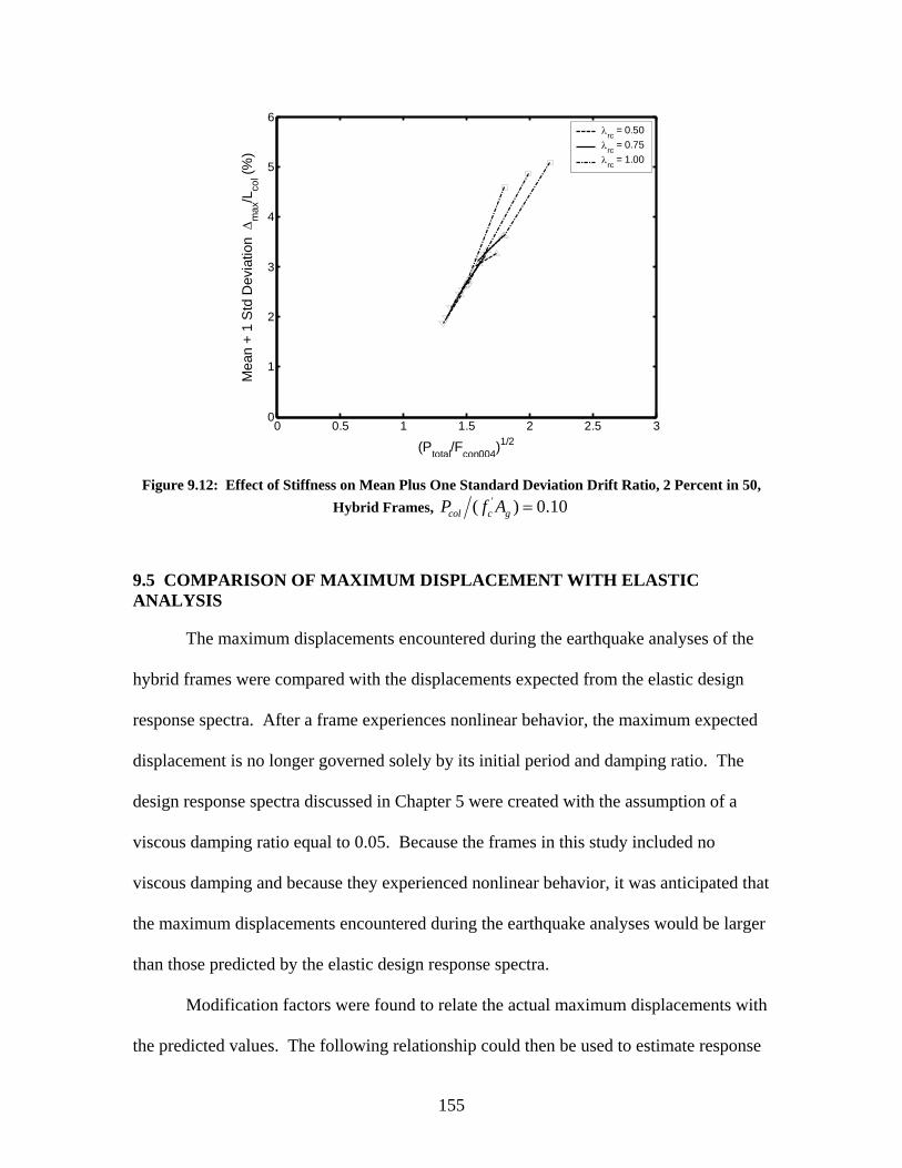
0 0.5 1 1.5 2 2.5 30
1
2
3
4
5
6
(Ptotal/Fcon004)1/2
Mea
n +
1 S
td D
evia
tion
Δm
ax/L
col (%
)
λrc = 0.50λrc = 0.75λrc = 1.00
Figure 9.12: Effect of Stiffness on Mean Plus One Standard Deviation Drift Ratio, 2 Percent in 50,
Hybrid Frames, '( ) 0.10col c gP f A =
9.5 COMPARISON OF MAXIMUM DISPLACEMENT WITH ELASTIC ANALYSIS
The maximum displacements encountered during the earthquake analyses of the
hybrid frames were compared with the displacements expected from the elastic design
response spectra. After a frame experiences nonlinear behavior, the maximum expected
displacement is no longer governed solely by its initial period and damping ratio. The
design response spectra discussed in Chapter 5 were created with the assumption of a
viscous damping ratio equal to 0.05. Because the frames in this study included no
viscous damping and because they experienced nonlinear behavior, it was anticipated that
the maximum displacements encountered during the earthquake analyses would be larger
than those predicted by the elastic design response spectra.
Modification factors were found to relate the actual maximum displacements with
the predicted values. The following relationship could then be used to estimate response
155
quantities for inelastic behavior without viscous damping:
=predicted dSψΔ (9.3)
where ψ = modification factor
= spectral displacement dS
The modification factor was calculated by averaging max dSΔ for all the frames as
shown in the following relationship:
max. .
1 1mean
frames motionsN N
ij d i motionsi j
frames
S N
Nψ
= =
⎡ ⎤⎛ ⎞Δ⎢ ⎥⎜ ⎟
⎢⎝ ⎠⎣=∑ ∑
⎥⎦ (9.4)
The modification factors for the 10 percent in 50 ground motions were found
from Equation 9.4 to be as follows:
o Frames with axial-load ratio equal to 0.05
• 1.43ψ = for the mean
• 1.73ψ = for the mean plus one standard deviation
o Frames with axial-load ratio equal to 0.10
• 1.30ψ = for the mean
• 1.53ψ = for the mean plus one standard deviation
For the 2 percent in 50 ground motions, the modification factors were found to be
as follows:
o Frames with axial-load ratio equal to 0.05
• 1.44ψ = for the mean
• 1.78ψ = for the mean plus one standard deviation
o Frame with axial-load ratio equal to 0.10
• 1.49ψ = for the mean
• 1.94ψ = for the mean plus one standard deviation
156
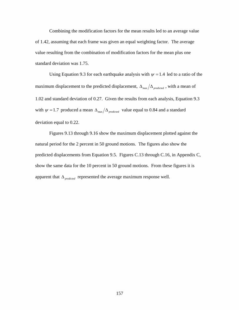
Combining the modification factors for the mean results led to an average value
of 1.42, assuming that each frame was given an equal weighting factor. The average
value resulting from the combination of modification factors for the mean plus one
standard deviation was 1.75.
Using Equation 9.3 for each earthquake analysis with 1.4ψ = led to a ratio of the
maximum displacement to the predicted displacement, max predictedΔ Δ , with a mean of
1.02 and standard deviation of 0.27. Given the results from each analysis, Equation 9.3
with 1.7ψ = produced a mean max predictedΔ Δ value equal to 0.84 and a standard
deviation equal to 0.22.
Figures 9.13 through 9.16 show the maximum displacement plotted against the
natural period for the 2 percent in 50 ground motions. The figures also show the
predicted displacements from Equation 9.5. Figures C.13 through C.16, in Appendix C,
show the same data for the 10 percent in 50 ground motions. From these figures it is
apparent that represented the average maximum response well. predictedΔ
157
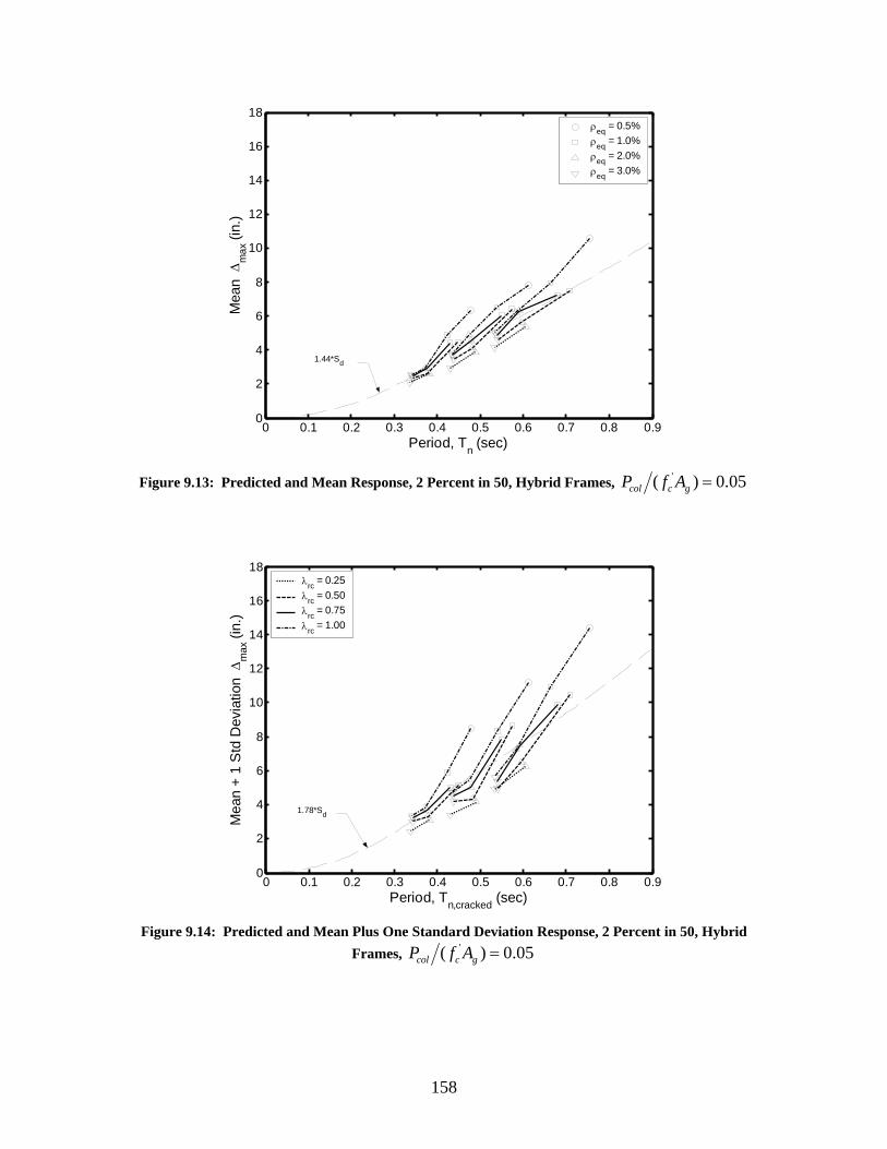
0 0.1 0.2 0.3 0.4 0.5 0.6 0.7 0.8 0.90
2
4
6
8
10
12
14
16
18
Period, Tn (sec)
Mea
n Δ
max
(in.
)
ρeq = 0.5%ρeq = 1.0%ρeq = 2.0%ρeq = 3.0%
1.44*Sd
Figure 9.13: Predicted and Mean Response, 2 Percent in 50, Hybrid Frames, '( ) 0.05col c gP f A =
0 0.1 0.2 0.3 0.4 0.5 0.6 0.7 0.8 0.90
2
4
6
8
10
12
14
16
18
Period, Tn,cracked (sec)
Mea
n +
1 S
td D
evia
tion
Δm
ax (i
n.)
λrc = 0.25λrc = 0.50λrc = 0.75λrc = 1.00
1.78*Sd
Figure 9.14: Predicted and Mean Plus One Standard Deviation Response, 2 Percent in 50, Hybrid
Frames, '( ) 0.05col c gP f A =
158
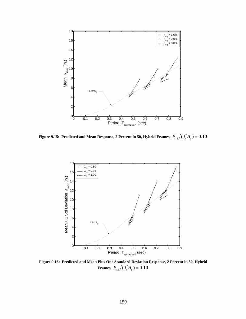
0 0.1 0.2 0.3 0.4 0.5 0.6 0.7 0.8 0.90
2
4
6
8
10
12
14
16
18
Period, Tn,cracked (sec)
Mea
n Δ
max
(in.
)
ρeq = 1.0%ρeq = 2.0%ρeq = 3.0%
1.49*Sd
Figure 9.15: Predicted and Mean Response, 2 Percent in 50, Hybrid Frames, '( ) 0.10col c gP f A =
0 0.1 0.2 0.3 0.4 0.5 0.6 0.7 0.8 0.90
2
4
6
8
10
12
14
16
18
Period, Tn,cracked (sec)
Mea
n +
1 S
td D
evia
tion
Δm
ax (i
n.)
λrc = 0.50λrc = 0.75λrc = 1.00
1.94*Sd
Figure 9.16: Predicted and Mean Plus One Standard Deviation Response, 2 Percent in 50, Hybrid
Frames, '( ) 0.10col c gP f A =
159
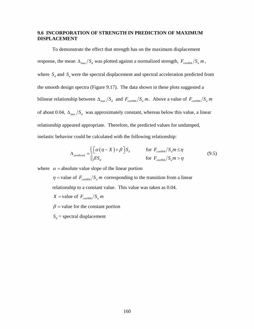
9.6 INCORPORATION OF STRENGTH IN PREDICTION OF MAXIMUM DISPLACEMENT
To demonstrate the effect that strength has on the maximum displacement
response, the mean max dSΔ was plotted against a normalized strength, 004con aF S m ,
where and were the spectral displacement and spectral acceleration predicted from
the smooth design spectra (Figure 9.17). The data shown in these plots suggested a
bilinear relationship between
dS aS
max dSΔ and 004con aF S m . Above a value of 004con aF S m
of about 0.04, max dSΔ was approximately constant, whereas below this value, a linear
relationship appeared appropriate. Therefore, the predicted values for undamped,
inelastic behavior could be calculated with the following relationship:
( ) 004
004
for
for d con a
predictedd co
X S F S m
S F n aS m
α η β η
β η
⎧⎡ ⎤− + ≤⎪⎣ ⎦Δ = ⎨>⎪⎩
(9.5)
where α = absolute value slope of the linear portion
η = value of 004con aF S m corresponding to the transition from a linear
relationship to a constant value. This value was taken as 0.04.
X = value of 004con aF S m
β = value for the constant portion
= spectral displacement dS
160
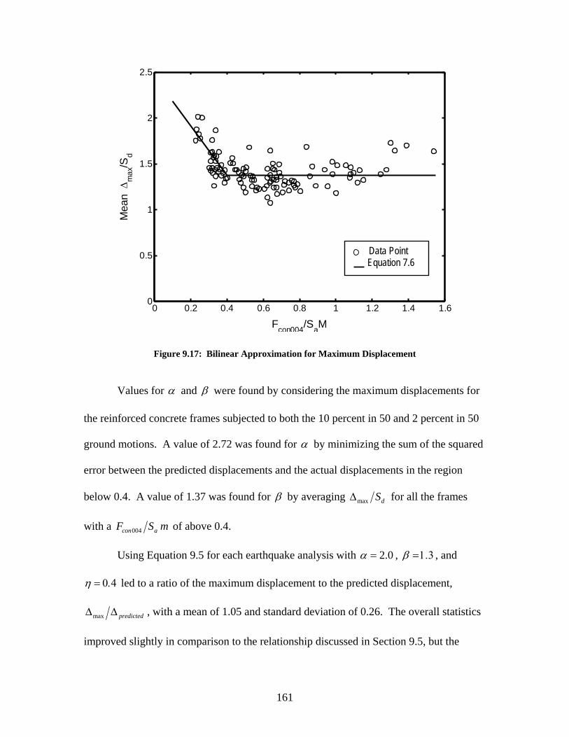
0 0.2 0.4 0.6 0.8 1 1.2 1.4 1.60
0.5
1
1.5
2
2.5
Fcon004/SaM
Mea
n Δ
max
/Sd
Data Point Equation 7.6
Figure 9.17: Bilinear Approximation for Maximum Displacement
Values for α and β were found by considering the maximum displacements for
the reinforced concrete frames subjected to both the 10 percent in 50 and 2 percent in 50
ground motions. A value of 2.72 was found for α by minimizing the sum of the squared
error between the predicted displacements and the actual displacements in the region
below 0.4. A value of 1.37 was found for β by averaging max dSΔ for all the frames
with a 004con aF S m of above 0.4.
Using Equation 9.5 for each earthquake analysis with 2.0α = , β =1.3 , and
η = 0.4 led to a ratio of the maximum displacement to the predicted displacement,
max predictedΔ Δ , with a mean of 1.05 and standard deviation of 0.26. The overall statistics
improved slightly in comparison to the relationship discussed in Section 9.5, but the
161
accuracy improved significantly for low values of the strength ratio. The predicted
response calculated from Equation 9.5 is shown in Figure 9.17.
9.7 TRENDS IN RESIDUAL DISPLACEMENT
After a frame has undergone yielding during ground motion excitation it may not
return to its initial equilibrium position. This difference in position before and after the
ground excitation has stopped is referred to as the residual displacement. Residual
displacements can affect whether a structure needs to be replaced or simply repaired.
Residual displacements were found for the 10 percent in 50 ground motions and the 2
percent in 50 ground motions.
The range of the maximum residual displacement resulting from the 10 percent in
50 ground motions was as follows:
o Frames with axial-load ratio equal to 0.05
• Minimum: 0.0 in. (numerous frames and ground motions,
max colLΔ = 0.00 percent)
• Maximum: 0.2 in. (frame 7.005.100, ground motion 10-3,
max colLΔ = 0.05 percent)
o Frames with axial-load ratio equal to 0.10
• Minimum: 0.0 in. (numerous frames and ground motions,
max colLΔ = 0.00 percent)
• Maximum: 0.3 in. (frame 7.020.0.50, ground motion 10-3,
max colLΔ = 0.09 percent)
For the 2 percent in 50 ground motions, the extreme value of the maximum
residual displacement was as follows:
o Frames with axial-load ratio equal to 0.05
• Minimum: 0.0 in. (numerous frames and ground motions,
162
max colLΔ = 0.00 percent)
• Maximum: 1.1 in. (frame 7.020.025, ground motion 2-3,
max colLΔ = 0.32 percent)
o Frame with axial-load ratio equal to 0.10
• Minimum: 0.0 in. (numerous frames and ground motions,
max colLΔ = 0.00 percent)
• Maximum: 1.5 in. (frame 7.030.050, ground motion 2-3, max colLΔ =0.45
percent)
As described in Chapter 7, the strain-hardening ratio and viscous damping ratio
selected to model the frame were found to significantly affect the resulting residual
displacements. Therefore, complete residual displacement results are not presented.
Nonetheless, the residual displacements for the hybrid frames tended to be smaller than
those for the reinforced concrete frames. Also, as expected, the residual displacements
generally decreased as the re-centering ratio increased. This suggests that prestressing
does help reduce residual displacement.
An additional conclusion discussed in Chapter 7 is that the maximum
displacements were not drastically affected by the strain-hardening ratio or viscous
damping ratio, providing additional confidence in the maximum displacements presented
in this document.
163
CHAPTER 10 SEISMIC PERFORMANCE EVALUATION
This chapter evaluates and compares the two proposed bridge systems by
investigating various deformation measures (such as displacement ductility) and limit
states (such as the onset of cover concrete spalling). Variations of the baseline reinforced
concrete frame and hybrid frame described in Chapter 4 were subjected to pushover
analyses and earthquake analyses. From the pushover analyses, key quantities such as
first yield properties, initial cracked properties, nominal yield displacement, and
maximum strength were calculated (chapters 6 and 8). The maximum displacements
resulting from 10 ground motions were computed during the earthquake analyses
(chapters 7 and 9). Some of these key quantities were utilized to provide further insight
into the response of the proposed systems, as well as to provide a basis for comparing and
contrasting the two proposed bridge systems.
Numerous states may occur when an axially loaded column is subjected to
flexure. These states are briefly described below.
1. Initial Cracking. Initial cracking corresponds to the first flexural cracking in the
column. After the column starts to crack, the stiffness decreases considerably.
This change between the cracked and uncracked stiffness was evident in the
results from the pushover analyses presented in chapters 6 and 8. Although
reaching the cracking limit state can significantly decrease stiffness, and in turn
affect the response of the frame during an earthquake, reaching the cracking limit
state generally does not result in the need for repairs because the crack widths are
small, and the cracks close at the end of the earthquake.
164
2. First Yield. First yield is reached when the column’s extreme tensile steel first
reaches its yield strain. When the column reaches first yield, the stiffness
continues to decrease. The ratio of first yield to full yield, or the yielding of all
tensile reinforcing steel, depends on the column geometry and the number of bars
in the column. For a rectangular section with only two layers of reinforcement,
this ratio is near 1.0 because all the tensile reinforcing steel typically yields at the
same time. This ratio is significantly smaller for a circular column because first
yield may occur when only one bar yields. The values for first yield are
summarized in chapters 6 and 8.
3. Onset of Cover Concrete Spalling. Significant deterioration of the cover concrete
can result in cover concrete spalling. For well-confined columns, cover concrete
spalling will generally not significantly affect the seismic resistance of the frame
(Priestley et al. 1996). The need for repair is commonly associated with the onset
of cover concrete spalling. Depending on the extent of the damage, the cost to
repair the bridge may be significant, and the bridge may be temporarily out of
service.
4. Onset of Bar Buckling. As the axial strain in the column’s core increases, the
concrete behaves nonlinearly, and more of the compression force, caused by the
column axial force and column moment, must be resisted by the longitudinal
reinforcing steel. Also, as the core expands under the axial load, lateral forces are
exerted on the longitudinal reinforcing steel. If the compression force and/or
lateral force become excessive, the longitudinal reinforcing bars may buckle
(Berry 2003). The onset of bar buckling generally requires expensive repairs and
165
possibly partial replacements, especially because bar buckling frequently causes
fracture of the spiral reinforcement. Safety also becomes a concern after the onset
of bar buckling, and the structure may be out of service for some time.
5. Fracture of Longitudinal Bars. Bar fracture can occur if the tensile strains in the
longitudinal reinforcing bars become excessive. Fracture at lower strain levels
can be precipitated by several cycles of alternating buckling and straightening.
As with bar buckling, rupture of a longitudinal bar can result in significant
damage that requires extensive repairs or replacement.
6. Ultimate Limit State. No unique definition exists for the ultimate limit state. In
some cases the term is used to correspond to a physical event, such as bar rupture,
whereas others have defined it as a significant loss of lateral resistance, such as a
20 percent decrease in lateral resistance from the maximum strength (Priestley et
al. 1996). The definition of the ultimate state assumed for this study is described
in Section 10.5. When the ultimate limit state is reached, the main concern is for
safety. The structure most likely will be severely damaged and will require costly
replacement. But it is important that enough reserve strength remains so that the
bridge will not collapse.
States 3 through 6 were investigated during this study and are discussed further in
later sections of this chapter. Section 10.1 presents results for displacement ductility,
which is a measure of the inelastic deformation demand on the frame. Then the onset of
cover concrete spalling (Section 10.2), the onset of bar buckling (Section 10.3), bar
fracture (Section 10.4), and the proximity to ultimate limit state (Section 10.5) are
166
addressed further. Section 10.6 discusses the sensitivity of the response quantities to the
varied frame parameters.
10.1 DISPLACEMENT DUCTILITY DEMAND
In this research ductility was defined as the deformation at a given state divided
by the deformation at nominal yield. For a frame with yield displacement, , and a
maximum expected displacement,
yΔ
maxΔ , the displacement ductility demand, μΔ , is
defined as:
max
y
μΔ
Δ=
Δ (10.1)
A detailed discussion of ductility demands on reinforced concrete structures was
provided by Paulay and Priestley (1992).
The yield displacements were calculated and summarized in chapters 6 and 8, and
the maximum displacements were calculated and summarized in chapters 7 and 9.
Displacement ductility demands were calculated for each combination of ground motion
with reinforced concrete frame and ground motion with hybrid frame, with axial-load
ratios equal to 0.05 and 0.10. The results for the displacement ductility are presented in
detail in Appendix D (tables D.1 through D.3). Extreme values of displacement ductility
demand corresponding to the 10 percent in 50 ground motions were as follows:
o Reinforced concrete frames
• Minimum: 0.5 (frame 6.030.05, ground motion 10-3)
• Maximum: 7.2 (frame 5.005.15, ground motion 10-5)
o Hybrid frames with axial-load ratio equal to 0.05
• Minimum: 0.5 (frame 7.030.100, ground motion 10-3)
• Maximum: 3.9 (frame 6.005.100, ground motion 10-5)
o Hybrid frames with axial-load ratio equal to 0.10
167
• Minimum: 0.8 (frame 5.030.075, ground motion 10-3)
• Maximum: 4.1 (frame 7.010.100, ground motion 10-3)
For the 2 percent in 50 ground motions, displacement ductility demand ranged as
follows:
o Reinforced concrete frames
• Minimum: 1.3 (frame 5.030.05, ground motion 2-1)
• Maximum: 17.2 (frame 7.005.10, ground motion 2-3)
o Hybrid frames with axial-load ratio equal to 0.05
• Minimum: 1.2 (frame 6.030.025, ground motion 2-3)
• Maximum: 12.1 (frame 7.005.100, ground motion 2-3)
o Hybrid frames with axial-load ratio equal to 0.10
• Minimum: 2.1 (frame 7.030.050, ground motion 2-4)
• Maximum: 13.8 (frame 6.010.100, ground motion 2-3)
Figure 10.1 presents the mean and the mean plus one standard deviation of the
displacement ductility for the reinforced concrete frames subjected to the 2 percent in 50
ground motions. Figures 10.2 and 10.3 present similar data for the hybrid frames with
axial-load ratios of 0.05 and 0.10, respectively. Appendix D contains the figures showing
the displacement ductility for the 10 percent in 50 ground motions (figures D.1 through
D.3). The general trends observed in displacement ductility for the 10 percent in 50
ground motions were similar to those apparent in the results for the 2 percent in 50
ground motions.
168
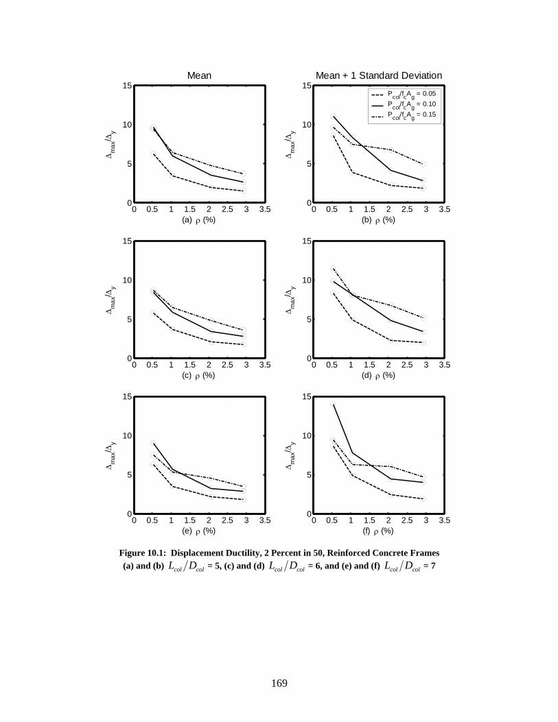
0 0.5 1 1.5 2 2.5 3 3.50
5
10
15
(a) ρ (%)
Δm
ax/ Δ
y
Mean
0 0.5 1 1.5 2 2.5 3 3.50
5
10
15
(c) ρ (%)
Δm
ax/ Δ
y
0 0.5 1 1.5 2 2.5 3 3.50
5
10
15
(e) ρ (%)
Δm
ax/ Δ
y
0 0.5 1 1.5 2 2.5 3 3.50
5
10
15
(b) ρ (%)
Δm
ax/ Δ
y
Mean + 1 Standard Deviation
Pcol/fcAg = 0.05Pcol/fcAg = 0.10Pcol/fcAg = 0.15
0 0.5 1 1.5 2 2.5 3 3.50
5
10
15
(d) ρ (%)
Δm
ax/ Δ
y
0 0.5 1 1.5 2 2.5 3 3.50
5
10
15
(f) ρ (%)
Δm
ax/ Δ
y
Figure 10.1: Displacement Ductility, 2 Percent in 50, Reinforced Concrete Frames (a) and (b) col colL D = 5, (c) and (d) col colL D = 6, and (e) and (f) col colL D = 7
169
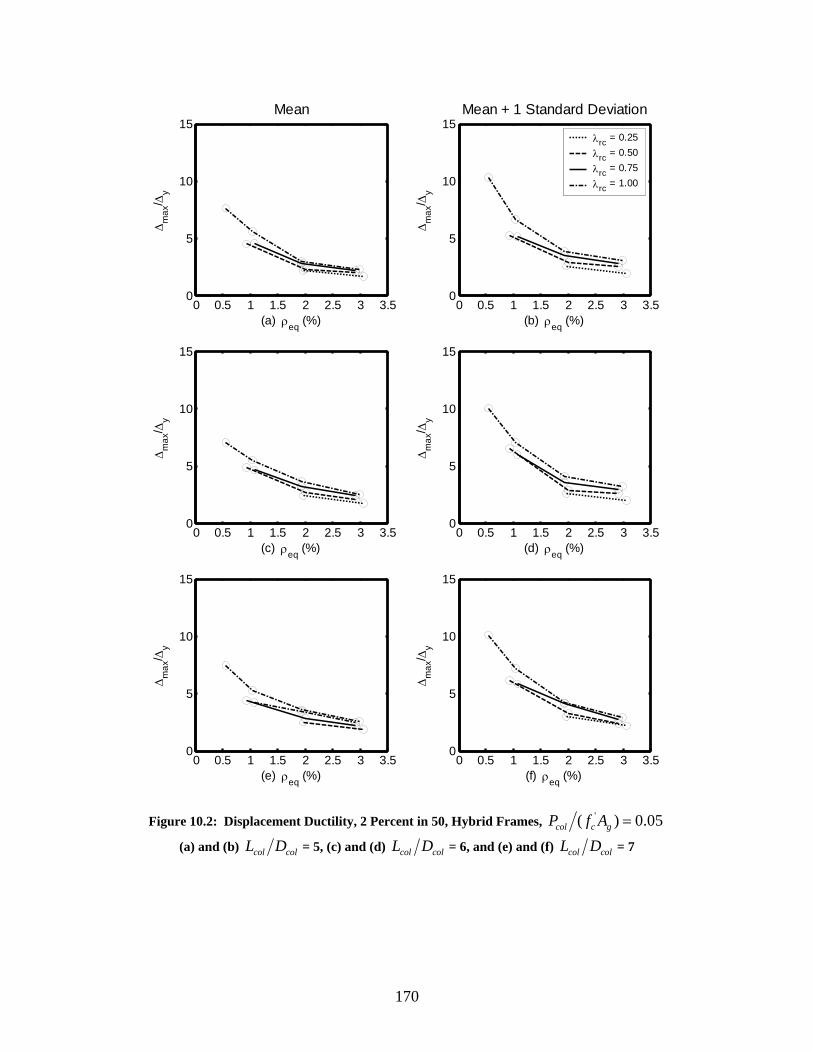
0 0.5 1 1.5 2 2.5 3 3.50
5
10
15
(a) ρeq (%)
Δm
ax/ Δ
y
Mean
0 0.5 1 1.5 2 2.5 3 3.50
5
10
15
(c) ρeq (%)
Δm
ax/ Δ
y
0 0.5 1 1.5 2 2.5 3 3.50
5
10
15
(e) ρeq (%)
Δm
ax/ Δ
y
0 0.5 1 1.5 2 2.5 3 3.50
5
10
15
(b) ρeq (%)
Δm
ax/ Δ
y
Mean + 1 Standard Deviation
λrc = 0.25λrc = 0.50λrc = 0.75λrc = 1.00
0 0.5 1 1.5 2 2.5 3 3.50
5
10
15
(d) ρeq (%)
Δm
ax/ Δ
y
0 0.5 1 1.5 2 2.5 3 3.50
5
10
15
(f) ρeq (%)
Δm
ax/ Δ
y
Figure 10.2: Displacement Ductility, 2 Percent in 50, Hybrid Frames, '( ) 0.05col c gP f A =
(a) and (b) col colL D = 5, (c) and (d) col colL D = 6, and (e) and (f) col colL D = 7
170
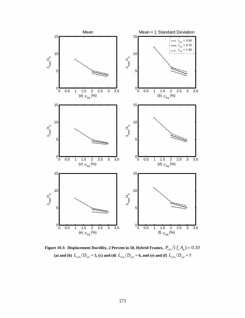
0 0.5 1 1.5 2 2.5 3 3.50
5
10
15
(a) ρeq (%)
Δm
ax/ Δ
y
Mean
0 0.5 1 1.5 2 2.5 3 3.50
5
10
15
(c) ρeq (%)
Δm
ax/ Δ
y
0 0.5 1 1.5 2 2.5 3 3.50
5
10
15
(e) ρeq (%)
Δm
ax/ Δ
y
0 0.5 1 1.5 2 2.5 3 3.50
5
10
15
(b) ρeq (%)
Δm
ax/ Δ
y
Mean + 1 Standard Deviation
λrc = 0.50λrc = 0.75λrc = 1.00
0 0.5 1 1.5 2 2.5 3 3.50
5
10
15
(d) ρeq (%)
Δm
ax/ Δ
y
0 0.5 1 1.5 2 2.5 3 3.50
5
10
15
(f) ρeq (%)
Δm
ax/ Δ
y
Figure 10.3: Displacement Ductility, 2 Percent in 50, Hybrid Frames, '( ) 0.10col c gP f A =
(a) and (b) col colL D = 5, (c) and (d) col colL D = 6, and (e) and (f) col colL D = 7
171
The data presented in figures 10.1 through 10.3 show the following trends:
• As the steel ratio, ρ or eqρ , increased, the displacement ductility demand
decreased. A greater rate of decrease occurred at smaller steel ratios, as is evident
in Figure 10.1 (a). This trend was expected because the earthquake analyses
indicated that the maximum displacement decreased as the steel ratio increased.
This trend is evident in each of the three figures.
• As the axial-load ratio, '(col c gP f A ) , increased, the displacement ductility demand
also increased. Figure 10.1 (c) illustrates this observation. Although some of the
lines cross one another, especially at low steel ratios, this is solely a result of the
frames that had numerical convergence problems. For most of the frames, the
maximum displacement was a consequence of ground motion 2-3. For those
frames, when the average values were calculated, they resulted in smaller average
values because they lacked the large contribution from ground motion 2-3
(Section 7.4). This observation was also expected because the earthquake
analyses revealed that as the axial-load ratio increased, and in turn the mass on the
frame increased, the maximum displacement and the cracked stiffness increased.
This observation indicates that the effect of the increased mass was larger than the
effect of the increased stiffness.
• The displacement ductility demand was not significantly influenced by col colL D .
This is evident by comparing figures 10.3 (a) and (e). The pushover analyses
showed that the yield displacement increased considerably with col colL D , but the
earthquake analyses showed that the maximum displacement also increased
significantly with col colL D . The insensitivity to col colL D suggests that the yield
172
displacement and the maximum displacement were influenced about equally by
the change in col colL D .
• For the hybrid frames, the displacement ductility was almost independent of the
re-centering ratio, rcλ . Figure 10.3 shows that the displacement ductility demand
increased slightly as the re-centering ratio increased. The small influence of the
re-centering ratio on displacement ductility was anticipated because the pushover
and earthquake analyses found that the re-centering ratio did not significantly
affect any of the results.
• A comparison of the mean displacement ductility of the hybrid frame with the
axial-load ratio, '(col c gP f A ) , equal to 0.10 (Figure 10.3) and that of the reinforced
concrete frame with the same axial-load ratio (Figure 10.1) showed that the
reinforced concrete frames had only slightly larger displacement ductility
demands than the hybrid frames.
• The mean plus one standard deviation was approximately 25 percent larger than
the mean values as is evident in each of the figures.
• The displacement ductility values for the 10 percent in 50 ground motions were
approximately half those for the 2 percent in 50 ground motions. The figures
illustrating the displacement ductility values for the 10 percent in 50 ground
motions can be found in Appendix D (figures D.1 through D.3).
173
10.2 ONSET OF COVER CONCRETE SPALLING
For well-confined reinforced concrete columns, the onset of cover concrete
spalling is typically the first flexural state that requires repairs that may put the bridge
temporarily out of service (Priestley et al. 1996).
Berry and Eberhard (2004) used 102 tests of rectangular columns and 40 spiral-
reinforced columns to develop a relationship for estimating a column’s displacement at
the onset of cover concrete spalling from known quantities such as column geometry,
reinforcing steel, and axial-load. Their relationship can also be used to estimate the
probability of cover concrete spalling for a given displacement. They defined the mean
displacement at the onset of cover concrete spalling using Equation 10.2.
'
1.6 1 1100 10
col col colspall
c g col
L P Lf A D
⎛ ⎞⎛ ⎞Δ = − +⎜ ⎟⎜⎜ ⎟⎝ ⎠⎝ ⎠
⎟ (10.2)
where column clear height between the top of the foundation and the bottom of the colL =
cap-beam
colP = compressive axial-load on a column
'cf = concrete compressive strength, taken as 5 ksi
gA = gross cross-sectional area of a column
colD = diameter of the column
Berry and Eberhard (2004) found that the probability of cover concrete spalling
occurring could be described as a function of the maximum displacement divided by the
estimated displacement at the onset of cover spalling given by Equation 10.2, max spallΔ Δ .
They found that for circular, reinforced concrete columns, the probability of the onset of
cover concrete spalling could be estimated from a normal cumulative density function
with a mean value of 1.07 and coefficient of variation, COV, equal to 0.352.
174
Equation 10.2 was developed from columns containing mild reinforcing steel
only, therefore it does not explicitly account for the prestressing steel included in the
hybrid frames of this study. To estimate the displacement at the onset of cover concrete
spalling for the hybrid frames, Equation 10.2 was modified so that was replaced by
the sum of the axial-load and the axial compression force caused by the prestressing steel,
. Although no experimental results were used to verify this assumption, this
modification was chosen because the only variable in Equation 10.2 that is directly
influenced by the addition of prestressing is the axial load. The sum of the axial-load and
the axial compression force caused by the prestressing steel was defined as follows:
colP
_col totalP
_col total col p g pP P A 0fρ= + (10.3)
where compressive axial-load on a column colP =
pρ = area of prestressing steel divided by the gross cross-sectional area of a
column, p gA A
gA = gross cross-sectional area of a column
0pf = stress in prestressing steel at zero drift, calculated as described in Chapter 8
For this study, the quantity max spallΔ Δ was found for each combination of frame
and ground motion, and from this value, the probability of the cover concrete spalling
was estimated from statistical information that Berry and Eberhard (2004) provided.
These estimated probabilities were conditional probabilities, meaning that they were the
estimated probability of cover concrete spalling initiating given the occurrence of a 10
percent in 50 or 2 percent in 50 earthquake event (Halder and Mahadevan 2000).
Complete results for the estimated probability of the onset of cover concrete spalling are
175
presented in tables E.4 through E.6 for the reinforced concrete frames and the hybrid
frames with axial-load ratios equal to 0.05 and 0.10. For the 10 percent in 50 ground
motions, the probability of onset of cover spalling ranged as follows:
o Reinforced concrete frames
• Minimum: 0.01 (frame 7.030.05, ground motion 10-3)
• Maximum: 0.88 (frame 5.005.15, ground motion 10-5)
o Hybrid frames with axial-load ratio equal to 0.05
• Minimum: 0.01 (numerous frames and ground motions)
• Maximum: 0.11 (frame 6.005.100, ground motion 10-5)
o Hybrid frames with axial-load ratio equal to 0.10
• Minimum: 0.01 (numerous frames and ground motions)
• Maximum: 0.24 (frame 7.010.100, ground motion 10-3)
The maximum values of the probability of cover spalling occurring listed above
may be a bit misleading. Note that these values are the maximum probability of cover
spalling occurring for individual ground motions, not mean values. Also note that the
relatively large value for the reinforced concrete frames is a result of an axial-load ratio
of 0.15, a value that was not considered for the hybrid frames. When individual frames
are compared with similar axial-load ratios and longitudinal reinforcement ratios, the
probabilities of cover concrete spalling occurring are more similar. For example, with an
axial-load ratio equal to 0.10, a column aspect ratio of 7, a reinforcement ratio of 0.10,
and ground motion 10-3, the probability of the onset of cover concrete spalling is equal to
0.25 for the reinforced concrete frame and 0.24 for the hybrid frame.
The probability of the occurrence of cover spalling ranged as follows for the 2
percent in 50 ground motions:
o Reinforced concrete frames
• Minimum: 0.03 (numerous frames and ground motions)
176
• Maximum: 1.00 (numerous frames and ground motions)
o Hybrid frames with axial-load ratio equal to 0.05
• Minimum: 0.02 (numerous frames and ground motions)
• Maximum: 0.99 (frame 7.005.100, ground motion 2-3)
o Hybrid frames with axial-load ratio equal to 0.10
• Minimum: 0.10 (numerous frames and ground motions)
• Maximum: 1.00 (numerous frames and ground motions)
For the reinforced concrete frames, the mean max spallΔ Δ and the mean probability
of the onset of cover concrete spalling are presented in Figure 10.4 for the 2 percent in 50
ground motions. Figures 10.5 and 10.6 show the same information for the hybrid frames
with axial-load ratios, '(col c gP f A ) , equal to 0.05 and 0.10, respectively. The results for
the 10 percent in 50 ground motions are plotted in Appendix D (figures D.4 through D.6).
The mean probability values were found by assuming that each ground motion had an
equal probability of occurrence.
177
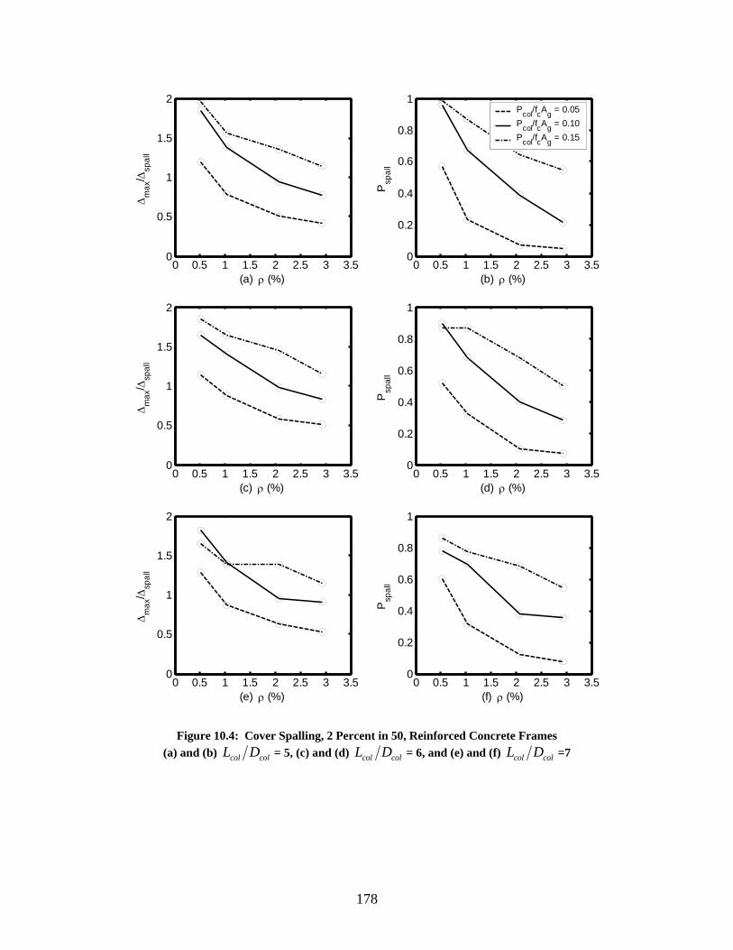
0 0.5 1 1.5 2 2.5 3 3.50
0.5
1
1.5
2
(a) ρ (%)
Δm
ax/ Δ
spal
l
0 0.5 1 1.5 2 2.5 3 3.50
0.5
1
1.5
2
(c) ρ (%)
Δm
ax/ Δ
spal
l
0 0.5 1 1.5 2 2.5 3 3.50
0.5
1
1.5
2
(e) ρ (%)
Δm
ax/ Δ
spal
l
0 0.5 1 1.5 2 2.5 3 3.50
0.2
0.4
0.6
0.8
1
(b) ρ (%)
Psp
all
Pcol/fcAg = 0.05Pcol/fcAg = 0.10Pcol/fcAg = 0.15
0 0.5 1 1.5 2 2.5 3
1
0.8
0.6
0.4
0.2
3.50
(d) ρ (%)
Psp
all
0 0.5 1 1.5 2 2.5 3
1
0.8
0.6
0.4
0.2
3.50
(f) ρ (%)
Psp
all
Figure 10.4: Cover Spalling, 2 Percent in 50, Reinforced Concrete Frames (a) and (b) col colL D = 5, (c) and (d) col colL D = 6, and (e) and (f) col colL D =7
178
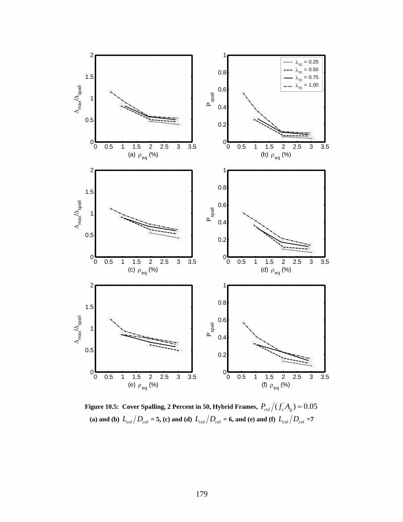
0 0.5 1 1.5 2 2.5 3 3.50
0.5
1
1.5
2
(a) ρeq (%)
Δm
ax/ Δ
spal
l
0 0.5 1 1.5 2 2.5 3 3.50
0.5
1
1.5
2
(c) ρeq (%)
Δm
ax/ Δ
spal
l
0 0.5 1 1.5 2 2.5 3 3.50
0.5
1
1.5
2
(e) ρeq (%)
Δm
ax/ Δ
spal
l
0 0.5 1 1.5 2 2.5 3 3.50
0.2
0.4
0.6
0.8
1
(b) ρeq (%)
Psp
all
λrc = 0.25λrc = 0.50λrc = 0.75λrc = 1.00
0 0.5 1 1.5 2 2.5 3 3.50
0.2
0.4
0.6
0.8
1
(d) ρeq (%)
Psp
all
0 0.5 1 1.5 2 2.5 3 3.50
0.2
0.4
0.6
0.8
1
(f) ρeq (%)
Psp
all
Figure 10.5: Cover Spalling, 2 Percent in 50, Hybrid Frames, '( ) 0.05col c gP f A =
(a) and (b) col colL D = 5, (c) and (d) col colL D = 6, and (e) and (f) col colL D =7
179
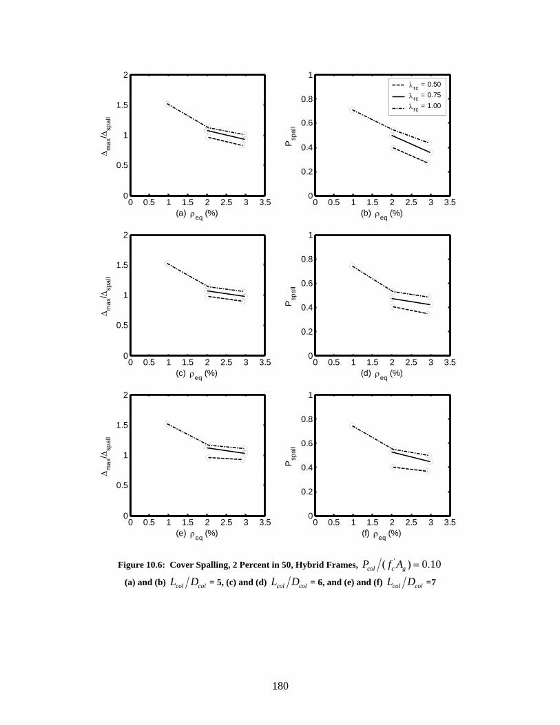
0 0.5 1 1.5 2 2.5 3 3.50
0.5
1
1.5
2
(a) ρeq (%)
Δm
ax/ Δ
spal
l
0 0.5 1 1.5 2 2.5 3 3.50
0.5
1
1.5
2
(c) ρeq (%)
Δm
ax/ Δ
spal
l
0 0.5 1 1.5 2 2.5 3 3.50
0.5
1
1.5
2
(e) ρeq (%)
Δm
ax/ Δ
spal
l
0 0.5 1 1.5 2 2.5 3 3.50
0.2
0.4
0.6
0.8
1
(b) ρeq (%)
Psp
all
λrc = 0.50λrc = 0.75λrc = 1.00
0 0.5 1 1.5 2 2.5 3 3.50
0.2
0.4
0.6
0.8
1
(d) ρeq (%)
Psp
all
0 0.5 1 1.5 2 2.5 3 3.50
0.2
0.4
0.6
0.8
1
(f) ρeq (%)
Psp
all
Figure 10.6: Cover Spalling, 2 Percent in 50, Hybrid Frames, '( ) 0.10col c gP f A =
(a) and (b) col colL D = 5, (c) and (d) col colL D = 6, and (e) and (f) col colL D =7
180
The results shown in Figures 10.4 through 10.6 indicate the following:
• As the steel ratio, ρ or eqρ , increased, the probability of cover concrete spalling
occurring decreased. A greater decrease occurred between smaller steel ratios, as
is evident in Figure 10.6 (b). This trend was anticipated because the earthquake
analyses revealed that the maximum displacement decreased as the steel ratio
increased. A smaller maximum displacement resulted in a smaller max spallΔ Δ ,
which in turn resulted in a smaller probability of the onset of cover concrete
spalling.
• As the axial-load ratio, '(col c gP f A ) , increased, the probability of cover concrete
spalling occurring also increased. Figure 10.4 (b) illustrates the observation.
Although some of the lines cross one another, such as in Figure 10.4 (d), this is
solely a result of the frames that had convergence problems. For most of the
frames, the maximum displacement was a consequence of ground motion 2-3.
For those frames, when the average values were calculated, they resulted in
smaller average values because they lacked the large contribution from ground
motion 2-3. This observation can be partially explained because the earthquake
analyses found that as the axial-load ratio increased, and in turn the mass on the
frame increased, the maximum displacement increased. In addition, it can be seen
from Equation 10.2 that as the axial-load ratio increased, spallΔ decreased.
Therefore, the increase in maxΔ and the decrease in spallΔ contributed to the
increase in the probability of cover concrete spalling occurring.
181
• The probability of the onset of cover spalling was not significantly influenced by
col colL D . This is evident by comparing between figures 10.6 (b) and (f). The
earthquake analyses showed that the maximum displacement increased
significantly as col colL D increased. Equation 10.2 indicates that spallΔ is also
influenced by col colL D , but not significantly.
• For the hybrid frames, the probability of cover concrete spalling occurring was
almost independent of the re-centering ratio, rcλ . A slight increase in the
probability of the onset of cover concrete spalling is shown in Figure 10.6 as the
re-centering ratio increased. The small influence of the re-centering ratio on
displacement ductility was anticipated because the pushover analyses and
earthquake analyses showed that the re-centering ratio did not significantly affect
any of the results. The variation in the probability of the occurrence of cover
concrete spalling could be partially explained by the modeling approximation of
using in Equation 10.2. _col totalP
• A comparison of the probability of cover concrete spalling occurring for the
hybrid frame with an axial-load ratio equal to 0.05 (Figure 10.5) and that of the
reinforced concrete frame with the same axial-load ratio (Figure 10.4) shows that
the two types of frames had similar probabilities. Closer inspection shows that
the reinforced concrete frame had slightly larger values than the hybrid frame.
• The results shown in figures 10.4 through 10.6 indicate that there was a
significant probability that the frames would experience spalling when subjected
to 2 percent in 50 seismic events. The values for the probability of the onset of
182
cover concrete spalling were approximately 1 5 as large for the 10 percent in 50
ground motions. Figures D.4 through D.6 in Appendix D illustrate the values for
the probability of cover concrete spalling occurring for the 10 percent in 50
ground motions.
10.3 ONSET OF BAR BUCKLING
The onset of bar buckling in a reinforced concrete column is especially
undesirable. Once it has occurred, extensive repairs are typically required to return the
bridge to service. If the damage is severe, repairing the columns may not be
economically or technically feasible, and all or part of the bridge will need to be replaced.
Berry and Eberhard (2004) developed a relationship for estimating the mean
displacement corresponding to the onset of bar buckling from known quantities such as
column geometry, amount of reinforcing steel, and axial-load. The probability of the
onset of bar buckling in the columns of the frames considered here was estimated from
the values provided in their work.
Berry and Eberhard (2004) developed Equation 10.4 for estimating the
displacement corresponding to the onset of bar buckling for circular, spiral-reinforced
columns as:
'
3.25 1 1 1100 10
col b col colbb bb eff
col c g col
L d PkD f A D
ρ⎛ ⎞⎛ ⎞ ⎛
Δ = + − +⎜ ⎟⎜ ⎟ ⎜⎜ ⎟⎝ ⎠ ⎝⎝ ⎠
L ⎞⎟⎠
(10.4)
where column clear height between the top of the foundation and the bottom of the colL =
cap-beam
bbk = taken as 150 for the circular, spiral-reinforced columns
effρ = 't y cf fρ where tρ is the ratio of volume of spiral reinforcement to total
183
volume of the core
bd = diameter of the longitudinal reinforcing bar
colD = diameter of the column
colP = compressive axial-load on a column
'cf = concrete compressive strength, taken as 5 ksi
gA = gross cross-sectional area of a column
Berry and Eberhard (2004) also found that the probability of the onset of bar
buckling could be calculated from the maximum displacement divided by the estimated
displacement at the onset of bar buckling given by Equation 10.4, max bbΔ Δ . They found
that for circular, reinforced concrete columns, the probability of the onset of bar buckling
could be estimated from a normal cumulative density function with a mean value of 0.97
and coefficient of variation, COV, equal to 0.246.
The equations presented in Berry and Eberhard (2004) were developed from
columns that contained mild reinforcing steel only; therefore, Equation 10.4 does not
explicitly account for the prestressing steel included in the hybrid frames of this study.
For the hybrid frames, Equation 10.4 was modified so that was replaced by the sum
of the axial-load and the axial compression force caused by the prestressing steel. The
relationship for this sum, , was given by Equation 10.3.
colP
_col totalP
For each combination of frame and ground motion, the quantity max bbΔ Δ was
found. From these results the probability of bar buckling occurring was estimated from
the normal cumulative density function. As with the probabilities discussed in Section
10.2, the estimated probabilities for the onset of bar buckling were conditional
probabilities, indicating that they were the probability of bar buckling initiating given the
184
occurrence of a 10 percent in 50 or 2 percent in 50 earthquake event (Halder and
Mahadevan 2000).
The results for the probability of the onset of bar buckling are summarized in
tables D.7 through D.9 in Appendix D. For the 10 percent in 50 ground motions the
probability of bar buckling initiating was essentially zero for all the frames studied. For
the 2 percent in 50 ground motions, the probability of bar buckling ranged as follows:
o Reinforced concrete frames
• Minimum: 0.00 (numerous frames and ground motions)
• Maximum: 0.67 (frame 7.005.15, ground motion 2-3)
o Hybrid frames with axial-load ratio equal to 0.05
• Minimum: 0.00 (most frames and ground motions)
• Maximum: 0.07 (frame 7.005.100, ground motion 2-3)
o Hybrid frames with axial-load ratio equal to 0.10
• Minimum: 0.00 (most frames and ground motions)
• Maximum: 0.25 (frame 6.010.100, ground motion 2-3)
For the reinforced concrete frames, the mean max bbΔ Δ and the mean probability
of bar buckling occurring are presented in Figure 10.7 for the 2 percent in 50 ground
motions. Figures 10.8 and 10.9 show the same information for the hybrid frames with
axial-load ratio equal to 0.05 and 0.10, respectively. These same results for the 10
percent in 50 ground motions may be found in figures D.7 through D.9 of Appendix D.
The mean probability values were found by assuming that each ground motion had an
equal probability of occurrence.
185
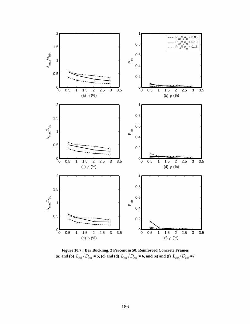
0 0.5 1 1.5 2 2.5 3 3.50
0.5
1
1.5
2
(a) ρ (%)
Δm
ax/ Δ
bb
0 0.5 1 1.5 2 2.5 3 3.50
0.5
1
1.5
2
(c) ρ (%)
Δm
ax/ Δ
bb
0 0.5 1 1.5 2 2.5 3 3.50
0.5
1
1.5
2
(e) ρ (%)
Δm
ax/ Δ
bb
0 0.5 1 1.5 2 2.5 3 3.50
0.2
0.4
0.6
0.8
1
(b) ρ (%)
Pbb
Pcol/fcAg = 0.05Pcol/fcAg = 0.10Pcol/fcAg = 0.15
0 0.5 1 1.5 2 2.5 3 3.50
0.2
0.4
0.6
0.8
1
(d) ρ (%)
Pbb
0 0.5 1 1.5 2 2.5 3 3.50
0.2
0.4
0.6
0.8
1
(f) ρ (%)
Pbb
Figure 10.7: Bar Buckling, 2 Percent in 50, Reinforced Concrete Frames (a) and (b) col colL D = 5, (c) and (d) col colL D = 6, and (e) and (f) col colL D =7
186
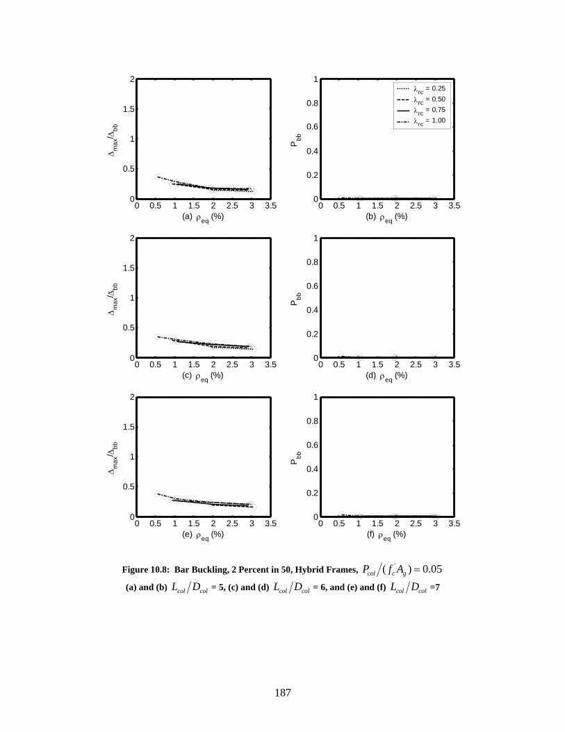
0 0.5 1 1.5 2 2.5 3 3.50
0.5
1
1.5
2
(a) ρeq (%)
Δm
ax/ Δ
bb
0 0.5 1 1.5 2 2.5 3 3.50
0.5
1
1.5
2
(c) ρeq (%)
Δm
ax/ Δ
bb
0 0.5 1 1.5 2 2.5 3 3.50
0.5
1
1.5
2
(e) ρeq (%)
Δm
ax/ Δ
bb
0 0.5 1 1.5 2 2.5 3 3.50
0.2
0.4
0.6
0.8
1
(b) ρeq (%)
Pbb
λrc = 0.25λrc = 0.50λrc = 0.75λrc = 1.00
0 0.5 1 1.5 2 2.5 3 3.50
0.2
0.4
0.6
0.8
1
(d) ρeq (%)
Pbb
0 0.5 1 1.5 2 2.5 3 3.50
0.2
0.4
0.6
0.8
1
(f) ρeq (%)
Pbb
Figure 10.8: Bar Buckling, 2 Percent in 50, Hybrid Frames, '( ) 0.05col c gP f A =
(a) and (b) col colL D = 5, (c) and (d) col colL D = 6, and (e) and (f) col colL D =7
187
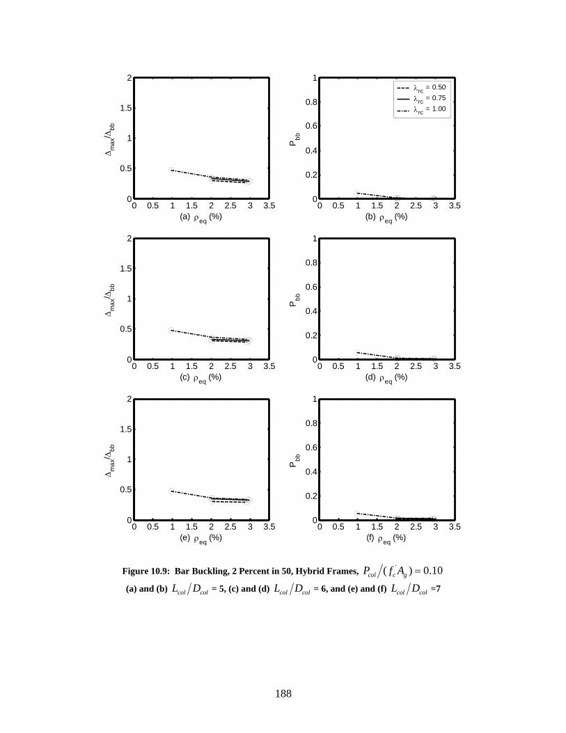
0 0.5 1 1.5 2 2.5 3 3.50
0.5
1
1.5
2
(a) ρeq (%)
Δm
ax/ Δ
bb
0 0.5 1 1.5 2 2.5 3 3.50
0.5
1
1.5
2
(c) ρeq (%)
Δm
ax/ Δ
bb
0 0.5 1 1.5 2 2.5 3 3.50
0.5
1
1.5
2
(e) ρeq (%)
Δm
ax/ Δ
bb
0 0.5 1 1.5 2 2.5 3 3.50
0.2
0.4
0.6
0.8
1
(b) ρeq (%)
Pbb
λrc = 0.50λrc = 0.75λrc = 1.00
0 0.5 1 1.5 2 2.5 3 3.50
0.2
0.4
0.6
0.8
1
(d) ρeq (%)
Pbb
0 0.5 1 1.5 2 2.5 3 3.50
0.2
0.4
0.6
0.8
1
(f) ρeq (%)
Pbb
Figure 10.9: Bar Buckling, 2 Percent in 50, Hybrid Frames, '( ) 0.10col c gP f A =
(a) and (b) col colL D = 5, (c) and (d) col colL D = 6, and (e) and (f) col colL D =7
188
The mean probability of bar buckling occurring remained below 0.15 for the
reinforced concrete frames and remained below 0.05 for the hybrid frames. The
following comments were noted from the results shown in figures 10.7 through 10.9.
• For small values of the steel ratio, the probability of the onset of bar buckling
decreased as the steel ratio, ρ or eqρ , increased, as observed in Figure 10.9. This
trend is consistent with the smaller maximum displacements encountered during
the earthquake analyses as the steel ratio increased. A smaller maximum
displacement resulted in a smaller max bbΔ Δ , which in turn resulted in a smaller
probability of bar buckling occurring.
• Because the probability of bar buckling occurring remained small, the axial-load
ratio, '(col c gP f A ) , was concluded to have an insignificant effect on the probability
of the onset of bar buckling. This observation is evident in each of the figures.
• The probability of bar buckling occurring was not significantly influenced by
col colL D . This is evident by comparing between figures 10.9 (b) and (f). This
observation is also evident from the plots of max bbΔ Δ shown in figures 10.7
through 10.9. The earthquake analyses found that the maximum displacement
increased significantly as col colL D increased. Equation 10.4 also indicates that
is influenced by bbΔ col colL D .
• For the hybrid frames, the probability of bar buckling occurring was not
significantly affected by the re-centering ratio, rcλ . This is evident from the plots
of max bbΔ Δ shown in the figures. For different values of rcλ , the results for
max bbΔ Δ fall on top of each other.
189
• A comparison of the max bbΔ Δ between the hybrid frame with an axial-load ratio
equal to 0.05 (Figure 10.8) and the reinforced concrete frame with the same axial-
load ratio (Figure 10.7) shows that the two types of frames had similar values.
• For the reinforced concrete frames, the results shown in Figure 10.7 indicate that
the probability of bar buckling occurring remained below 0.15 for frames with
low longitudinal reinforcement ratios and remained below 0.05 for frames with
high reinforcement ratios when they were subjected to 2 percent in 50 seismic
events. The results shown in figures 10.8 and 10.9 indicate that the probability of
bar buckling occurring remained below 0.05 for all the hybrid frames. The values
for the probability of the onset of bar buckling were nearly zero for all frames
subjected to the 10 percent in 50 ground motions. Figures D.7 through D.9 in
Appendix D illustrate the values for the probability of bar buckling for the 10
percent in 50 ground motions.
• Note that for hybrid frames, the strain in the mild steel is highly dependent on the
chosen unbonded length. When a hybrid frame is designed, the necessary
unbonded length can be chosen so that the mild steel does not exceed a chosen
level of strain.
10.4 MAXIMUM STRAIN IN LONGITUDINAL MILD STEEL
Although strain hardening was included in the mild reinforcing steel used in the
frames studied, as described in Chapter 4, bar fracture was not modeled. As the tensile
strain in the longitudinal reinforcing steel increases, the potential for bar rupture also
increases significantly. Although strain at bar rupture varies depending on the grade of
190
the bar, the bar diameter, hysteretic loading, and the manufacturer, Nawy (2000)
suggested a range of 0.05 and 0.12 for the fracture strain for an 8-in. gage length.
For this study, a steel strain threshold of 0.05 was selected. In frames that
contained longitudinal reinforcing steel that suffered strains higher than this value, bar
rupture was deemed possible. The strains encountered during the earthquake analyses are
summarized in the tables of Appendix D (tables D.10 through D.12). During the
earthquake analyses with the 10 percent in 50 ground motions, the maximum strain in the
longitudinal mild steel ranged as follows:
o Reinforced concrete frames
• Minimum: 0.001 (frame 6.030.05, ground motion 10-3)
• Maximum: 0.057 (frame 5.005.15, ground motion 10-5)
o Hybrid frames with axial-load ratio equal to 0.05
• Minimum: 0.001 (numerous frames and ground motions)
• Maximum: 0.022 (frame 6.005.100, ground motion 10-5)
o Hybrid frames with axial-load ratio equal to 0.10
• Minimum: 0.002 (numerous frames and ground motions)
• Maximum: 0.016 (frame 6.010.100, ground motion 10-5)
The maximum strain in the longitudinal mild steel ranged as follows for the 2
percent in 50 ground motions:
o Reinforced concrete frames
• Minimum: 0.002 (frame 5.020.15, ground motion 2-3)
• Maximum: 0.106 (frame 5.005.10, ground motion 2-5)
o Hybrid frames with axial-load ratio equal to 0.05
• Minimum: 0.003 (numerous frames and ground motions)
• Maximum: 0.037 (frame 5.005.100, ground motion 2-5)
o Hybrid frames with axial-load ratio equal to 0.10
• Minimum: 0.006 (frame 6.030.100, ground motion 2-3)
• Maximum: 0.033 (frame 5.010.100, ground motion 2-5)
191

For the reinforced concrete frames, the mean maximum strain in the extreme
tensile steel, stlε , and the mean plus one standard deviation are presented in Figure 10.10
for the 2 percent in 50 ground motions. The same information is shown in figures 10.11
and 10.12 for the hybrid frames with axial-load ratios equal to 0.05 and 0.10,
respectively. Figures D.10 through D.12, found in Appendix D, illustrate the same
information for the 10 percent in 50 ground motions.
192
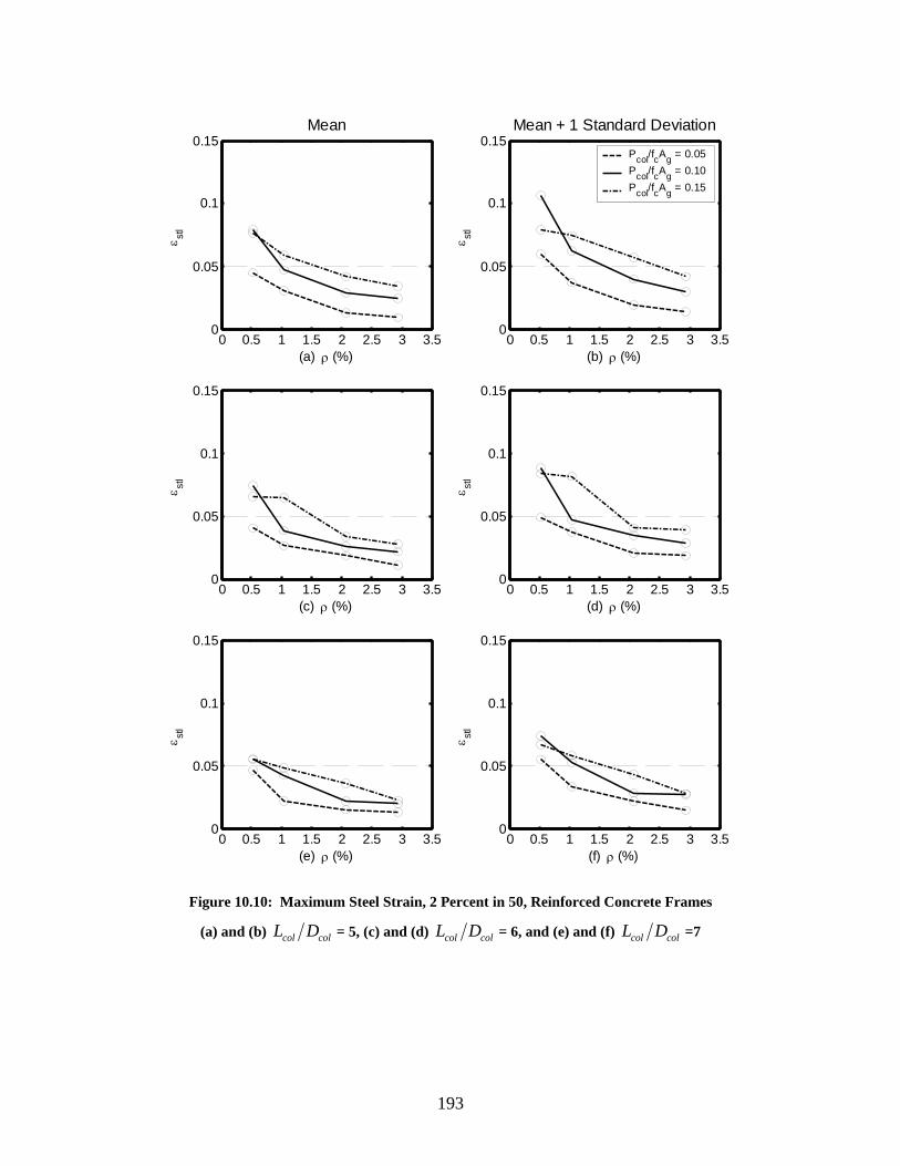
0 0.5 1 1.5 2 2.5 3 3.50
0.05
0.1
0.15
(a) ρ (%)
ε stl
Mean
0 0.5 1 1.5 2 2.5 3 3.50
0.05
0.1
0.15
(c) ρ (%)
ε stl
0 0.5 1 1.5 2 2.5 3 3.50
0.05
0.1
0.15
(e) ρ (%)
ε stl
0 0.5 1 1.5 2 2.5 3 3.50
0.05
0.1
0.15
(b) ρ (%)
ε stl
Mean + 1 Standard Deviation
Pcol/fcAg = 0.05Pcol/fcAg = 0.10Pcol/fcAg = 0.15
0 0.5 1 1.5 2 2.5 3 3.50
0.05
0.1
0.15
(d) ρ (%)
ε stl
0 0.5 1 1.5 2 2.5 3 3.50
0.05
0.1
0.15
(f) ρ (%)
ε stl
Figure 10.10: Maximum Steel Strain, 2 Percent in 50, Reinforced Concrete Frames
(a) and (b) col colL D = 5, (c) and (d) col colL D = 6, and (e) and (f) col colL D =7
193
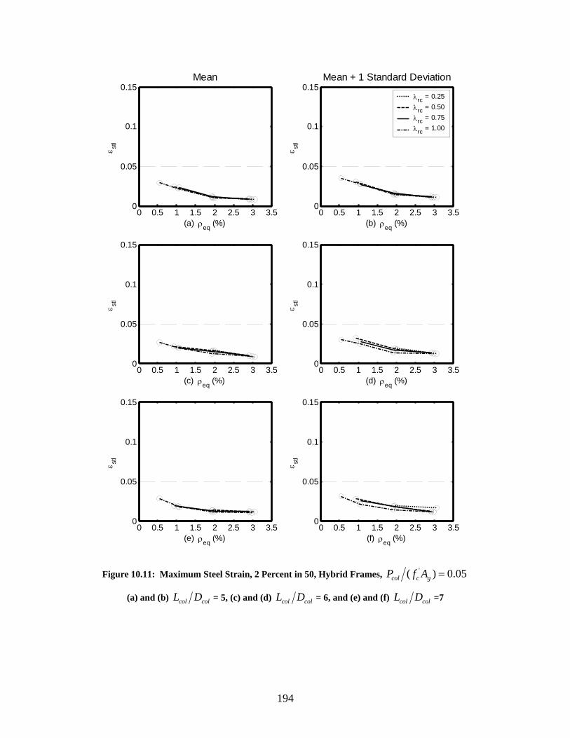
0 0.5 1 1.5 2 2.5 3 3.50
0.05
0.1
0.15
(a) ρeq (%)
ε stl
Mean
0 0.5 1 1.5 2 2.5 3 3.50
0.05
0.1
0.15
(c) ρeq (%)
ε stl
0 0.5 1 1.5 2 2.5 3 3.50
0.05
0.1
0.15
(e) ρeq (%)
ε stl
0 0.5 1 1.5 2 2.5 3 3.50
0.05
0.1
0.15
(b) ρeq (%)
ε stl
Mean + 1 Standard Deviation
λrc = 0.25λrc = 0.50λrc = 0.75λrc = 1.00
0 0.5 1 1.5 2 2.5 3 3.50
0.05
0.1
0.15
(d) ρeq (%)
ε stl
0 0.5 1 1.5 2 2.5 3 3.50
0.05
0.1
0.15
(f) ρeq (%)
ε stl
Figure 10.11: Maximum Steel Strain, 2 Percent in 50, Hybrid Frames, '( ) 0.05col c gP f A =
(a) and (b) col colL D = 5, (c) and (d) col colL D = 6, and (e) and (f) col colL D =7
194
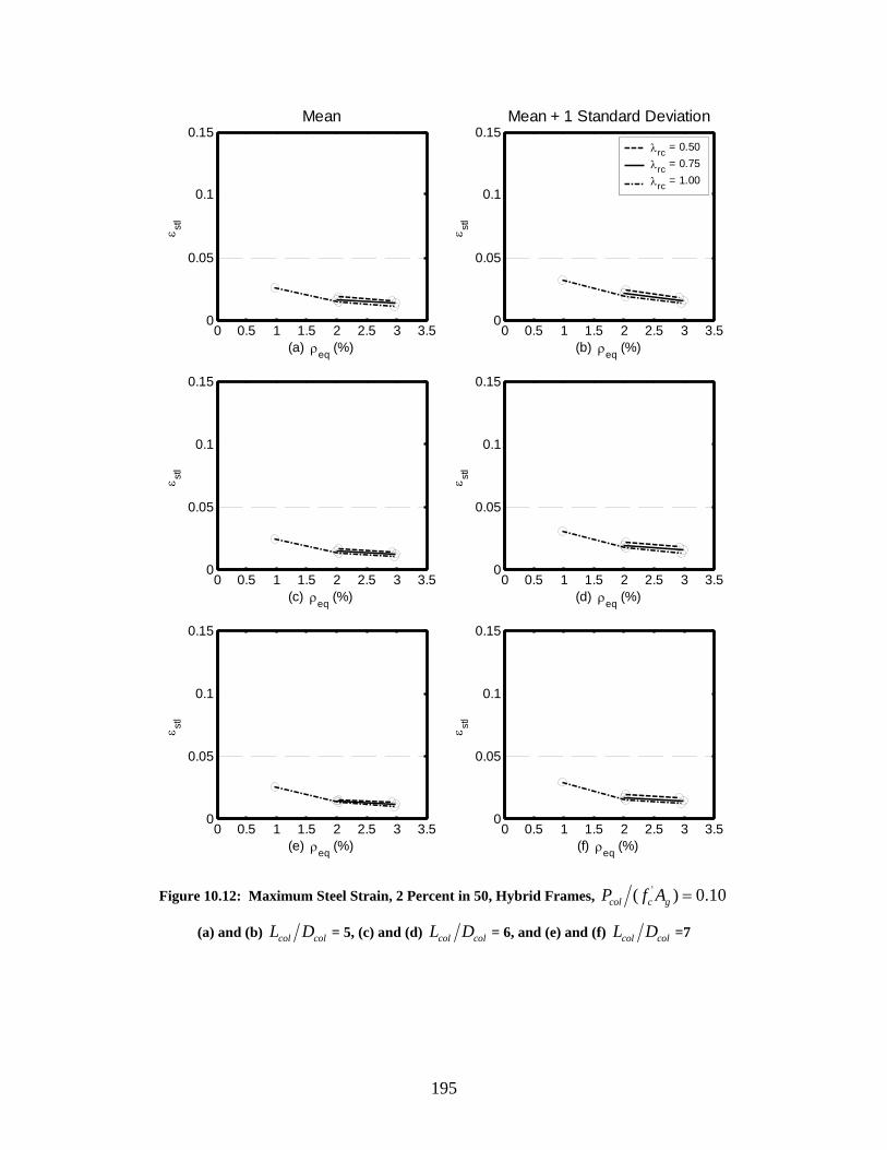
0 0.5 1 1.5 2 2.5 3 3.50
0.05
0.1
0.15
(a) ρeq (%)
ε stl
Mean
0 0.5 1 1.5 2 2.5 3 3.50
0.05
0.1
0.15
(c) ρeq (%)
ε stl
0 0.5 1 1.5 2 2.5 3 3.50
0.05
0.1
0.15
(e) ρeq (%)
ε stl
0 0.5 1 1.5 2 2.5 3 3.50
0.05
0.1
0.15
(b) ρeq (%)
ε stl
Mean + 1 Standard Deviation
λrc = 0.50λrc = 0.75λrc = 1.00
0 0.5 1 1.5 2 2.5 3 3.50
0.05
0.1
0.15
(d) ρeq (%)
ε stl
0 0.5 1 1.5 2 2.5 3 3.50
0.05
0.1
0.15
(f) ρeq (%)
ε stl
Figure 10.12: Maximum Steel Strain, 2 Percent in 50, Hybrid Frames, '( ) 0.10col c gP f A =
(a) and (b) col colL D = 5, (c) and (d) col colL D = 6, and (e) and (f) col colL D =7
195
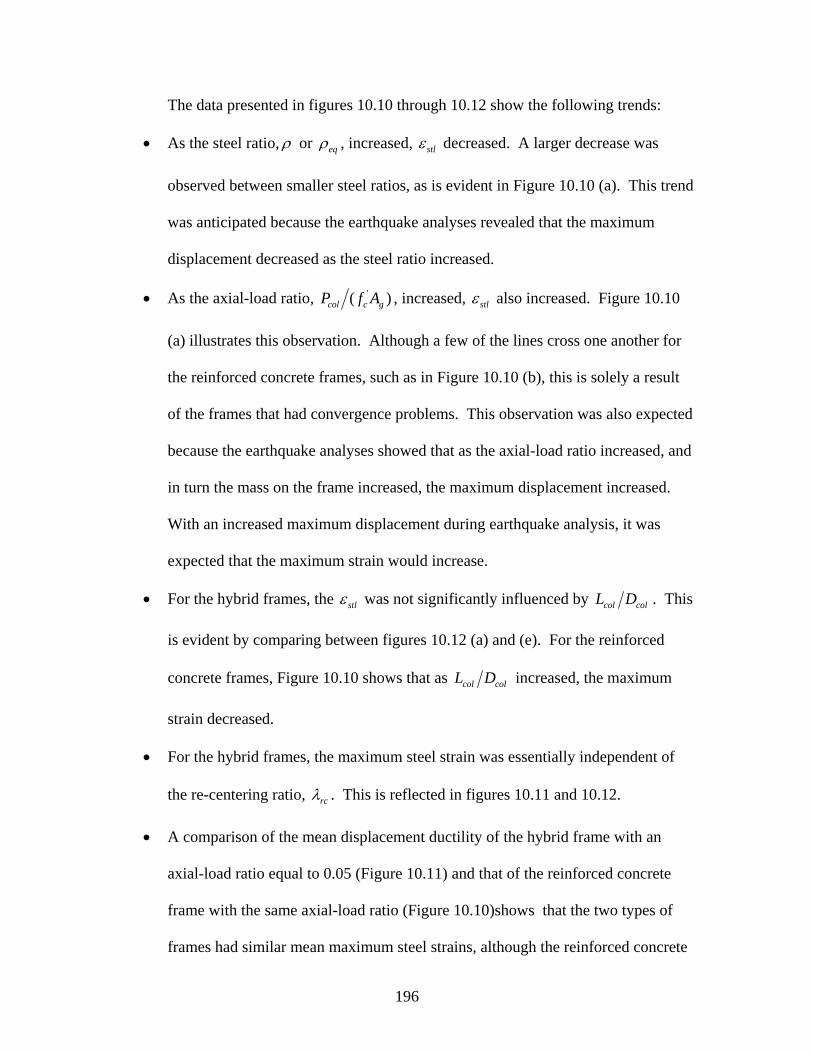
The data presented in figures 10.10 through 10.12 show the following trends:
• As the steel ratio, ρ or eqρ , increased, stlε decreased. A larger decrease was
observed between smaller steel ratios, as is evident in Figure 10.10 (a). This trend
was anticipated because the earthquake analyses revealed that the maximum
displacement decreased as the steel ratio increased.
• As the axial-load ratio, '(col c gP f A ) , increased, stlε also increased. Figure 10.10
(a) illustrates this observation. Although a few of the lines cross one another for
the reinforced concrete frames, such as in Figure 10.10 (b), this is solely a result
of the frames that had convergence problems. This observation was also expected
because the earthquake analyses showed that as the axial-load ratio increased, and
in turn the mass on the frame increased, the maximum displacement increased.
With an increased maximum displacement during earthquake analysis, it was
expected that the maximum strain would increase.
• For the hybrid frames, the stlε was not significantly influenced by col colL D . This
is evident by comparing between figures 10.12 (a) and (e). For the reinforced
concrete frames, Figure 10.10 shows that as col colL D increased, the maximum
strain decreased.
• For the hybrid frames, the maximum steel strain was essentially independent of
the re-centering ratio, rcλ . This is reflected in figures 10.11 and 10.12.
• A comparison of the mean displacement ductility of the hybrid frame with an
axial-load ratio equal to 0.05 (Figure 10.11) and that of the reinforced concrete
frame with the same axial-load ratio (Figure 10.10)shows that the two types of
frames had similar mean maximum steel strains, although the reinforced concrete
196
frames had a slightly larger stlε than the hybrid frames. These figures also show
that the mean plus one standard deviation was significantly larger for the
reinforced concrete frames than for the hybrid frames. The figures indicate that
bar rupture could be a serious concern for the reinforced concrete frames when
exposed to a 2 percent in 50 event, especially for higher axial-load ratios. The
partial debonding of the mild reinforcing steel in the hybrid frames explains the
relatively lower stlε found in the hybrid frames.
• The mean plus one standard deviation was approximately 25 percent larger than
the mean values for the reinforced concrete frames, as is evident in Figure 10.10.
The mean plus one standard deviation was essentially the same as the mean
values for the hybrid frames.
• The stlε values were approximately 30 to 40 percent smaller for the 10 percent in
50 ground motions for the reinforced concrete frames. For the hybrid frames, the
stlε values were approximately 50 to 60 percent smaller for the 10 percent in 50
ground motions. Figures D.10 through D.12 in Appendix D illustrate the stlε
values for the 10 percent in 50 ground motions .
10.5 PROXIMITY TO ULTIMATE DISPLACEMENT
No unique definition exists for the ultimate limit state because typically some
amount of residual strength remains in a well-confined frame, even after a significant loss
of strength occurs during a pushover analysis (Preistley et al. 1996). For this study, the
displacement at the ultimate limit state, ultΔ , was defined as the state that existed when
the first of the following two events occurred:
197
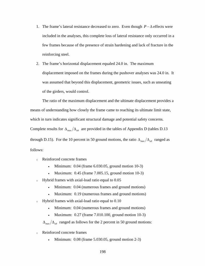
1. The frame’s lateral resistance decreased to zero. Even though effects were
included in the analyses, this complete loss of lateral resistance only occurred in a
few frames because of the presence of strain hardening and lack of fracture in the
reinforcing steel.
P − Δ
2. The frame’s horizontal displacement equaled 24.0 in. The maximum
displacement imposed on the frames during the pushover analyses was 24.0 in. It
was assumed that beyond this displacement, geometric issues, such as unseating
of the girders, would control.
The ratio of the maximum displacement and the ultimate displacement provides a
means of understanding how closely the frame came to reaching its ultimate limit state,
which in turn indicates significant structural damage and potential safety concerns.
Complete results for max ultΔ Δ are provided in the tables of Appendix D (tables D.13
through D.15). For the 10 percent in 50 ground motions, the ratio max ultΔ Δ ranged as
follows:
o Reinforced concrete frames
• Minimum: 0.04 (frame 6.030.05, ground motion 10-3)
• Maximum: 0.45 (frame 7.005.15, ground motion 10-3)
o Hybrid frames with axial-load ratio equal to 0.05
• Minimum: 0.04 (numerous frames and ground motions)
• Maximum: 0.19 (numerous frames and ground motions)
o Hybrid frames with axial-load ratio equal to 0.10
• Minimum: 0.04 (numerous frames and ground motions)
• Maximum: 0.27 (frame 7.010.100, ground motion 10-3)
max ultΔ Δ ranged as follows for the 2 percent in 50 ground motions:
o Reinforced concrete frames
• Minimum: 0.08 (frame 5.030.05, ground motion 2-3)
198
• Maximum: 1.19 (frame 7.005.10, ground motion 2-3), this was the only
value above 1.00 and indicates that this frame exceeded its ultimate limit
state as defined in this section.
o Hybrid frames with axial-load ratio equal to 0.05
• Minimum: 0.07 (numerous frames and ground motions)
• Maximum: 0.72 (frame 7.005.100, ground motion 2-3)
o Hybrid frames with axial-load ratio equal to 0.10
• Minimum: 0.15 (numerous frames and ground motions)
• Maximum: 0.84 (frame 7.010.100, ground motion 2-5)
For the reinforced concrete frames, the mean values for max ultΔ Δ and the mean
plus one standard deviation are presented in Figure 10.13 for the 2 percent in 50 ground
motions. The same information is presented in figures 10.14 and 10.15 for the hybrid
frames with axial-load ratio equal to 0.05 and 0.10, respectively. Similar data are
presented in figures D.13 through D.15 in Appendix D for the 10 percent in 50 ground
motions.
199
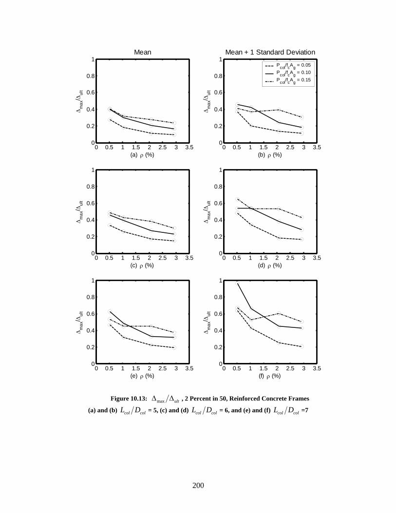
0 0.5 1 1.5 2 2.5 3 3.50
0.2
0.4
0.6
0.8
1
(a) ρ (%)
Δm
ax/ Δ
ult
Mean
0 0.5 1 1.5 2 2.5 3 3.50
0.2
0.4
0.6
0.8
1
(c) ρ (%)
Δm
ax/ Δ
ult
0 0.5 1 1.5 2 2.5 3 3.50
0.2
0.4
0.6
0.8
1
(e) ρ (%)
Δm
ax/ Δ
ult
0 0.5 1 1.5 2 2.5 3 3.50
0.2
0.4
0.6
0.8
1
(b) ρ (%)
Δm
ax/ Δ
ult
Mean + 1 Standard Deviation
Pcol/fcAg = 0.05Pcol/fcAg = 0.10Pcol/fcAg = 0.15
0 0.5 1 1.5 2 2.5 3 3.50
0.2
0.4
0.6
0.8
1
(d) ρ (%)
Δm
ax/ Δ
ult
0 0.5 1 1.5 2 2.5 3 3.50
0.2
0.4
0.6
0.8
1
(f) ρ (%)
Δm
ax/ Δ
ult
Figure 10.13: max ultΔ Δ , 2 Percent in 50, Reinforced Concrete Frames
(a) and (b) col colL D = 5, (c) and (d) col colL D = 6, and (e) and (f) col colL D =7
200

0 0.5 1 1.5 2 2.5 3 3.50
0.2
0.4
0.6
0.8
1
(a) ρeq (%)
Δm
ax/ Δ
ult
Mean
0 0.5 1 1.5 2 2.5 3 3.50
0.2
0.4
0.6
0.8
1
(c) ρeq (%)
Δm
ax/ Δ
ult
0 0.5 1 1.5 2 2.5 3 3.50
0.2
0.4
0.6
0.8
1
(e) ρeq (%)
Δm
ax/ Δ
ult
0 0.5 1 1.5 2 2.5 3 3.50
0.2
0.4
0.6
0.8
1
(b) ρeq (%)
Δm
ax/ Δ
ult
Mean + 1 Standard Deviation
λrc = 0.25λrc = 0.50λrc = 0.75λrc = 1.00
0 0.5 1 1.5 2 2.5 3 3.50
0.2
0.4
0.6
0.8
1
(d) ρeq (%)
Δm
ax/ Δ
ult
0 0.5 1 1.5 2 2.5 3 3.50
0.2
0.4
0.6
0.8
1
(f) ρeq (%)
Δm
ax/ Δ
ult
Figure 10.14: max ultΔ Δ , 2 Percent in 50, Hybrid Frames, '( ) 0.05col c gP f A =
(a) and (b) col colL D = 5, (c) and (d) col colL D = 6, and (e) and (f) col colL D =7
201
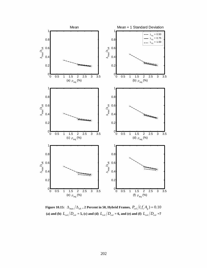
0 0.5 1 1.5 2 2.5 3 3.50
0.2
0.4
0.6
0.8
1
(a) ρeq (%)
Δm
ax/ Δ
ult
Mean
0 0.5 1 1.5 2 2.5 3 3.50
0.2
0.4
0.6
0.8
1
(c) ρeq (%)
Δm
ax/ Δ
ult
0 0.5 1 1.5 2 2.5 3 3.50
0.2
0.4
0.6
0.8
1
(e) ρeq (%)
Δm
ax/ Δ
ult
0 0.5 1 1.5 2 2.5 3 3.50
0.2
0.4
0.6
0.8
1
(b) ρeq (%)
Δm
ax/ Δ
ult
Mean + 1 Standard Deviation
λrc = 0.50λrc = 0.75λrc = 1.00
0 0.5 1 1.5 2 2.5 3 3.50
0.2
0.4
0.6
0.8
1
(d) ρeq (%)
Δm
ax/ Δ
ult
0 0.5 1 1.5 2 2.5 3 3.50
0.2
0.4
0.6
0.8
1
(f) ρeq (%)
Δm
ax/ Δ
ult
Figure 10.15: max ultΔ Δ , 2 Percent in 50, Hybrid Frames, '( ) 0.10col c gP f A =
(a) and (b) col colL D = 5, (c) and (d) col colL D = 6, and (e) and (f) col colL D =7
202
From figures 10.13 through 10.15 the following observations were made.
Because the ultimate displacement equaled 24 in. for all the frames except for three
reinforced concrete frames, these observations essentially reflect the trends and
observations for the maximum displacements presented in chapters 7 and 9.
• As the steel ratio, ρ or eqρ , increased, max ultΔ Δ decreased. The results also
suggest that a larger decrease occurred between smaller steel ratios, as is evident
in Figure 10.14 (e). This trend is consistent with the decreased maximum
displacement encountered during the earthquake analyses as the steel ratio
increased.
• As the axial-load ratio, '(col c gP f A ) , increased, max ultΔ Δ also increased. This
observation is illustrated in Figure 10.13 (a). Although a few of the lines cross
one another for the reinforced concrete frames, such as in Figure 10.13 (e), this is
a result of the mean values calculated without the contribution from frames that
had convergence problems. This trend was anticipated because the earthquake
analyses found that as the axial-load ratio increased, and in turn the mass on the
frame increased, the maximum displacement increased.
• As col colL D increased, max ultΔ Δ also increased. This is evident in each of the
figures. The earthquake analyses showed that as col colL D increased the
maximum displacement also increased, which corresponds to the trend observed
for max ultΔ Δ .
• For the hybrid frames, max ultΔ Δ was nearly independent of the re-centering ratio,
rcλ , which is the same trend observed in maximum displacement, as described in
203
chapters 7 and 9. This is reflected in figures 10.14 and 10.15.
• A comparison of the mean displacement ductility of the hybrid frame with an
axial-load ratio equal to 0.05 (Figure 10.14) and that of the reinforced concrete
frame with the same axial-load ratio and longitudinal reinforcement ratio (Figure
10.13) shows that the two types of frames had almost identical max ultΔ Δ values.
• The mean plus one standard deviation was approximately 40 percent larger than
the mean values, as reflected in the figures.
• The max ultΔ Δ values for the 10 percent in 50 ground motions were approximately
half those for the 2 percent in 50 ground motions. Figures illustrating the
max ultΔ Δ values for the 10 percent in 50 ground motions can be found in
Appendix D (figures D.13 through D.15).
10.6 SENSITIVITY OF PERFORMANCE TO FRAME PARAMETERS
This section summarizes the sensitivity of the response and performance
evaluation quantities, discussed in chapters 6 through 10, to variation of the frame
parameters. The responses of the reinforced concrete and hybrid frames were computed
for the following baseline values:
o column aspect ratio, 6col colL D =
o longitudinal reinforcement ratio, 0.01ρ = ( eqρ for hybrid frames)
o axial-load ratio, '( ) 0.05col c gP f A =
o re-centering ratio, 1.00rcλ = (for hybrid frames).
Table 10.1 summarizes the results of the response and performance evaluation
quantities for the reinforced concrete and hybrid frames with these baseline values. This
table also summarizes the percentage of change between the two types of frames. The
204
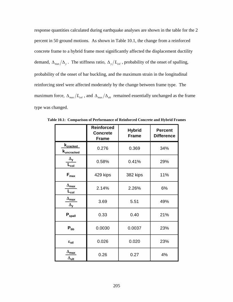
response quantities calculated during earthquake analyses are shown in the table for the 2
percent in 50 ground motions. As shown in Table 10.1, the change from a reinforced
concrete frame to a hybrid frame most significantly affected the displacement ductility
demand, max yΔ Δ . The stiffness ratio, y colLΔ , probability of the onset of spalling,
probability of the onset of bar buckling, and the maximum strain in the longitudinal
reinforcing steel were affected moderately by the change between frame type. The
maximum force, max colLΔ , and max ultΔ Δ remained essentially unchanged as the frame
type was changed.
Table 10.1: Comparison of Performance of Reinforced Concrete and Hybrid Frames
Reinforced Concrete
Frame
Hybrid Frame
Percent Difference
kcracked
kuncracked0.276 0.369 34%
Δy
Lcol0.58% 0.41% 29%
Fmax 429 kips 382 kips 11%
Δmax
Lcol2.14% 2.26% 6%
Δmax
Δy3.69 5.51 49%
Pspall 0.33 0.40 21%
Pbb 0.0030 0.0037 23%
εstl 0.026 0.020 23%
Δmax
Δult0.26 0.27 4%
205
To investigate the sensitivity of the calculated responses to the frame parameters,
individual parameters of the baseline frame were varied while the remaining parameters
were held fixed at the values selected for the baseline frame. The parameters were varied
as follows:
o column aspect ratio, col colL D , from 5 to 7
o longitudinal reinforcement ratio, ρ or eqρ , from 0.005 to 0.020
o axial-load ratio, '(col c gP f A ) , from 0.05 to 0.10
o re-centering ratio, rcλ , from 0.50 to 1.00.
Table 10.2 presents the percentage of increase or decrease in the response
quantities as each individual parameter was varied for the reinforced concrete frames.
Table 10.3 contains the same information for the hybrid frames. The response quantities
calculated during earthquake analyses are shown in tables 10.2 and 10.3 for the 2 percent
in 50 ground motions. The values contained in these tables were calculated from the
tables included in chapters 6 through 10 and their associated appendices.
As shown in tables 10.2 and 10.3, varying col colL D from 5 to 7 had a significant
effect on and bbP max ultΔ Δ . The percentage of change in was large because the
values of were small, below 0.01. As
bbP
bbP col colL D varied from 5 to 7, a moderate
change occurred in y colLΔ , , maxF max colLΔ , spallP , and stlε . Both the stiffness ratio and
the displacement ductility demand were essentially independent of col colL D .
206
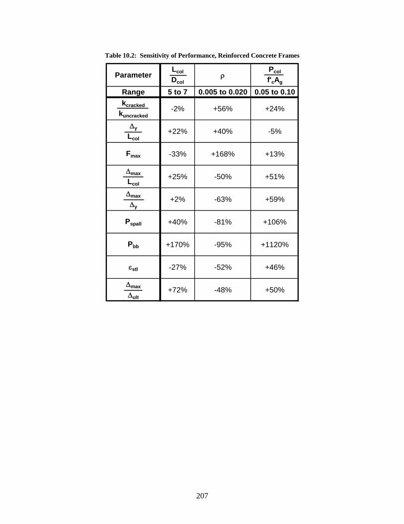
Table 10.2: Sensitivity of Performance, Reinforced Concrete Frames
ParameterLcol
Dcolρ
Pcol
f'cAg
Range 5 to 7 0.005 to 0.020 0.05 to 0.10kcracked
kuncracked-2% +56% +24%
Δy
Lcol+22% +40% -5%
Fmax -33% +168% +13%
Δmax
Lcol+25% -50% +51%
Δmax
Δy+2% -63% +59%
Pspall +40% -81% +106%
Pbb +170% -95% +1120%
εstl -27% -52% +46%
Δmax
Δult+72% -48% +50%
207
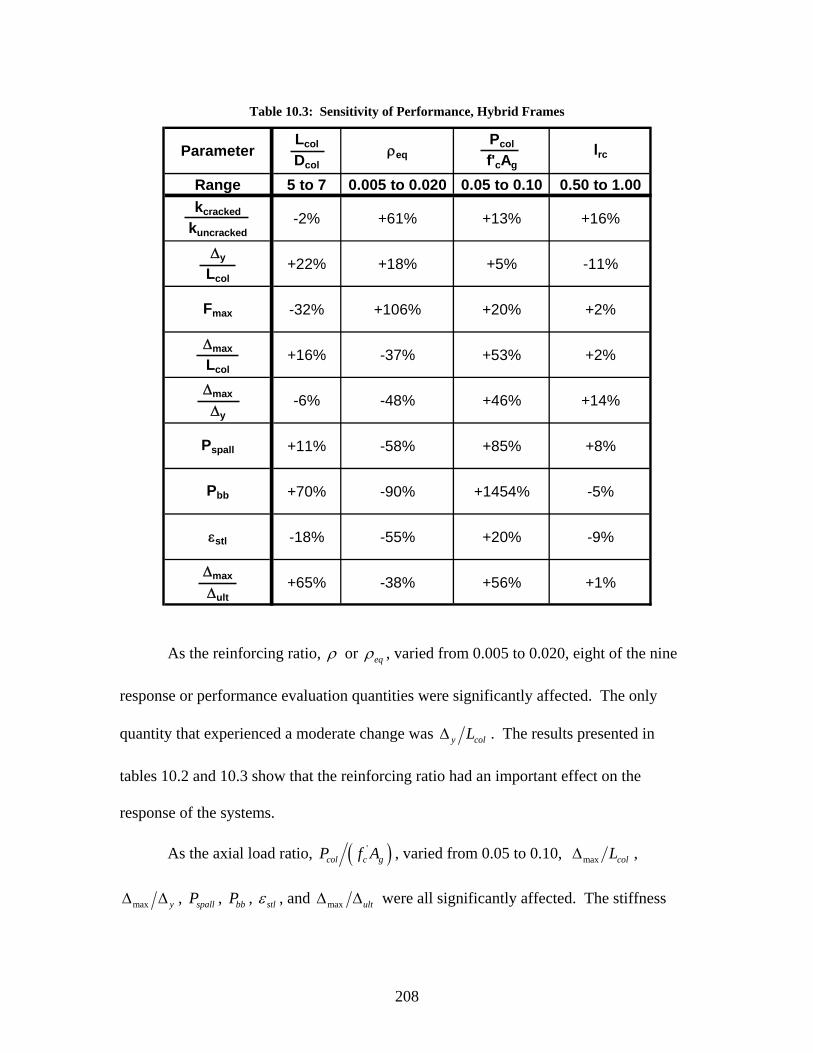
Table 10.3: Sensitivity of Performance, Hybrid Frames
ParameterLcol
Dcolρeq
Pcol
f'cAglrc
Range 5 to 7 0.005 to 0.020 0.05 to 0.10 0.50 to 1.00kcracked
kuncracked-2% +61% +13% +16%
Δy
Lcol+22% +18% +5% -11%
Fmax -32% +106% +20% +2%
Δmax
Lcol+16% -37% +53% +2%
Δmax
Δy-6% -48% +46% +14%
Pspall +11% -58% +85% +8%
Pbb +70% -90% +1454% -5%
εstl -18% -55% +20% -9%
Δmax
Δult+65% -38% +56% +1%
As the reinforcing ratio, ρ or eqρ , varied from 0.005 to 0.020, eight of the nine
response or performance evaluation quantities were significantly affected. The only
quantity that experienced a moderate change was y colLΔ . The results presented in
tables 10.2 and 10.3 show that the reinforcing ratio had an important effect on the
response of the systems.
As the axial load ratio, ( )'col c gP f A , varied from 0.05 to 0.10, max colLΔ ,
max yΔ Δ , spallP , , bbP stlε , and max ultΔ Δ were all significantly affected. The stiffness
208

ratio was moderately affected as the axial-load ratio varied, whereas y colLΔ and
were effectively independent of the change in axial-load ratio.
maxF
As shown in Table 10.3, as the re-centering ratio, rcλ , varied from 0.50 to 1.00,
little change occurred in the response or performance evaluation quantities.
209
CHAPTER 11 SUMMARY, CONCLUSIONS, AND RECOMMENDATIONS
11.1 SUMMARY
The country’s aging transportation infrastructure is subjected to ever-increasing
traffic volumes, and it must be continuously renewed and improved. Today, construction
operations that follow traditional practices lead to unacceptable traffic congestion,
pollution, and economic loss (Shahawy 2003).
The Federal Highway Administration (FHWA), the American Association of
State Highway and Transportation Officials (AASHTO), and many state departments of
transportation have been working to accelerate the construction process and reduce the
negative impacts of transportation construction on the traveling public.
The focus of this study was on the feasibility of using precast concrete pier
systems for the rapid construction of bridges in seismic regions. Potential benefits
include reduced traffic impacts caused by transportation construction, improved work
zone safety, reduced environmental impacts, improved constructability, increased quality,
and lowered life-cycle costs, providing benefits for bridge owners, designers, contractors,
and the traveling public. A review of previous systems and applications of precast
concrete components used for rapid bridge construction is summarized in Chapter 2 and
in Hieber et al. (2004). The study described in this report focused on the development
and evaluation of precast concrete bridge pier systems for use in the seismically active
region of Western Washington State.
This study evaluated the potential of two precast concrete bridge pier systems; the
first was a precast concrete emulation of a cast-in-place, reinforced concrete frame, and
210
the second was a precast hybrid frame (Chapter 3). Both systems consisted of a precast
concrete cap-beam and precast concrete columns supported on cast-in-place concrete
foundations. Components in the reinforced concrete system were connected with mild
steel deformed bars grouted or cast into ducts or openings. In the hybrid system, the
components were connected with deformed bars grouted or cast into ducts or openings, as
well as with unbonded prestressing strand. The prestressing strand was anchored in the
foundation, threaded through a duct located in the center of the column’s cross section,
and attached in the column-to-cap-beam connection. The hybrid system offered the
additional benefit of reducing the residual displacement by re-centering the system after a
seismic event.
The object-oriented analysis framework OpenSees (2000) was used to create
nonlinear finite element models representing individual precast concrete bridge piers
(Chapter 4). A parametric study, involving pushover analyses (chapters 6 and 8) and
earthquake analyses (chapters 7 and 9) of 36 reinforced concrete frames and 57 hybrid
frames, was conducted to quantify response characteristics and investigate the global
seismic response of various configurations of the proposed systems. The following
parameters were varied during the study:
o column aspect ratio, col colL D
o longitudinal reinforcement ratio, s gA Aρ = (reinforced concrete frames)
o equivalent reinforcement ratio, ( )eq s y p py yf f fρ ρ ρ= + (hybrid frames)
o axial-load ratio, '( )col c gP f A
o re-centering ratio, ( )0rc col p p s yP A f A fλ = + (hybrid frames).
During the earthquake analyses, each of the 36 reinforced concrete frames and 57
hybrid frames was subjected to five ground motions representing events with a 10 percent
211
probability of exceedance in 50 years (10 percent in 50) and five ground motions
representing events with a 2 percent probability of exceedance in 50 years (2 percent in
50), resulting in a total of 930 earthquake analyses performed during the parametric
study. The development of the ground motions is described in Chapter 5.
The results of the parametric study were used to develop a method for estimating
the response of the precast systems on the basis of an elastic design displacement
response spectrum (sections 7.5 and 9.5). In addition, the following performance
measures were used to evaluate the systems (Chapter 10):
o displacement ductility demand, μΔ
o probability of cover concrete spalling, spallP
o probability of bar buckling, bbP
o maximum strain in longitudinal mild steel, stlε (related to bar fracture)
o proximity to ultimate limit state, max ultΔ Δ .
11.2 CONCLUSIONS FROM SYSTEM DEVELOPMENT
To be considered for use, any alternative to the current cast-in-place concrete pier
system would need to possess numerous characteristics. Through an intensive literature
review and numerous discussions with WSDOT engineers, local precast concrete
producers, and local contractors, important attributes were identified. The following is a
list of the essential qualities of a feasible precast concrete bridge pier system for use in
Western Washington State.
• Connections are central to the seismic performance and constructability of precast
systems. Connections should be carefully designed, detailed, and constructed to
ensure adequate performance of the system. Limiting the required number of
212
connections is key to reducing the on-site construction effort. Connections
between components should provide acceptable construction tolerances.
• Fabrication, transportation, and erection weight limits, as well as length limits,
should be considered. The WSDOT Bridge Design Manual (WSDOT 2002)
suggests 180,000 lbs.
• Reducing the required quantity of cast-in-place concrete and formwork
significantly increases the benefit provided by a potential system.
• The system should be versatile to allow its use on a variety of bridge geometries
and configurations.
• The precast concrete system should be economically competitive with its cast-in-
place counterpart, but the comparison should include the value of time.
• The system should be durable to ensure quality construction and reduce life-cycle
costs.
11.3 CONCLUSIONS FROM THE PUSHOVER ANALYSES
The pushover analyses summarized in chapters 6 and 8, as well as in the tables of
Section 10.6, revealed the following:
• As described in Section 10.6, the difference between the reinforced concrete
frames and hybrid frames was around 30 percent for the stiffness ratio and
y colLΔ . The maximum force, , was essentially independent of frame type. maxF
• As col colL D varied, a moderate change occurred in y colLΔ and . The
stiffness ratio was essentially independent of
maxF
col colL D .
213
• As the reinforcing ratio, ρ or eqρ , varied, both the stiffness ratio and were
significantly affected. The only quantity that experienced a moderate change was
maxF
y colLΔ .
• The stiffness ratio was moderately affected as the axial-load ratio, '( )col c gP f A ,
varied whereas y colLΔ and were effectively independent of the change in
axial-load ratio.
maxF
• For the hybrid frames, as the re-centering ratio, rcλ , varied, little change occurred
in the pushover response quantities.
11.4 CONCLUSIONS FROM THE EARTHQUAKE ANALYSES
The earthquake analyses indicated the following:
• Maximum drift ratio, max colLΔ , significantly increased as the axial-load ratio,
'(col c gP f A ) , increased. The maximum drift ratio increased moderately with the
column aspect ratio, col colL D . An increase in longitudinal reinforcement ratio,
ρ or eqρ , resulted in a significant decrease in max colLΔ . These three behaviors
are consistent with results from an elastic single-degree-of-freedom system. The
first implies a larger seismic mass and the second a lower stiffness, both of which
lead to a longer period and larger displacement. An increased ρ causes an
increase in the cracked stiffness and a consequent reduction in peak displacement.
The maximum drift ratio was nearly independent of the re-centering ratio, rcλ .
• As a consequence of residual displacements encountered during the study, it was
concluded that the viscous damping ratio and the strain hardening ratio
214
incorporated in the nonlinear finite element model significantly affected the
residual displacements. Although detailed results were not presented in the study,
in general it was found that as rcλ increased, the residual displacement decreased.
This reinforces conclusions drawn by other studies related to hybrid frames (Sakai
and Mahin 2004 and Kwan and Billington 2003(b)).
A practical method was developed for estimating maximum seismic
displacements on the basis of the cracked section properties of the columns, the elastic
design displacement response spectrum, , and base-shear strength ratio. The
maximum displacement of the proposed systems, with no viscous damping included, was
predicted well with the following relationship:
dS
( ) 004
004
for
for d con a
predictedd co
X S F S m
S F n aS m
α η β η
β η
⎧⎡ ⎤− + ≤⎪⎣ ⎦Δ = ⎨>⎪⎩
(11.1)
where α = absolute value slope of the linear portion, taken as 2.0.
η = value of 004con aF S m corresponding to the transition from a linear
relationship to a constant value. This value was taken as 0.04.
X = value of 004con aF S m
β = value for the constant portion, taken as 1.3.
= spectral displacement dS
For the reinforced concrete frames, use of Equation 11.1 with 2.0α = , β =1.3 ,
and η = 0.4 for each earthquake analysis produced a ratio of the maximum displacement
computed with OpenSees to the predicted displacement computed with Equation 11.1,
max predictedΔ Δ , with a mean of 0.98 and standard deviation of 0.25. For the hybrid
215
frames, use of Equation 11.1 for each earthquake analysis resulted in a mean of 1.05 and
standard deviation of 0.26.
11.5 CONCLUSIONS FROM THE SEISMIC PERFORMANCE EVALUATION
With the results obtained from the earthquake analyses, a performance evaluation
was carried out to estimate the level of expected damage.
For the 10 percent in 50 ground motions, this study found moderate probabilities
of the onset of cover concrete spalling, minimal probabilities of the onset of bar buckling,
and very low values of maximum strain in the longitudinal reinforcement. For example,
at an axial-load ratio of 0.10 and longitudinal reinforcement ratio of 0.01, the mean
probability of cover concrete spalling occurring was 0.12 for the reinforced concrete
frames and 0.10 for the hybrid frames. The mean probability of bar buckling occurring
was 0.0005 for the reinforced concrete and hybrid frames. For the same conditions, the
mean maximum strain in the longitudinal mild steel was 0.015 for the reinforced concrete
frames and 0.012 for the hybrid frames.
For the 2 percent in 50 ground motions, this study found significant probabilities
of cover concrete spalling occurring, minimal probabilities of bar buckling occurring, and
moderate maximum strains in the longitudinal reinforcement. For example, at an axial-
load ratio of 0.10 and longitudinal reinforcement ratio of 0.01, the mean probability of
cover concrete spalling occurring was 0.68 for the reinforced concrete frames and 0.73
for the hybrid frames. The mean probability of bar buckling occurring was 0.04 for the
reinforced concrete and hybrid frames. For this same axial-load ratio and reinforcement
ratio, the mean maximum strain in the longitudinal mild steel was 0.042 for the
reinforced concrete frames and 0.025 for the hybrid frames.
216
The performance evaluation described in Chapter 10 indicated the following:
• The displacement ductility demand was influenced by the steel ratio, ρ or eqρ ,
and decreased as the steel ratio increased. The displacement ductility demand
significantly increased with the axial-load ratio, '(col c gP f A ) and was effectively
independent of the column aspect ratio, col colL D . For the hybrid frames, as the
re-centering ratio, rcλ , increased, the displacement ductility was essentially
unchanged. The reinforced concrete frames had slightly larger displacement
ductility demands than the hybrid frames.
• The probability of cover concrete spalling decreased significantly as the steel
ratio, ρ or eqρ , increased and increased significantly as the axial-load ratio,
'(col c gP f A ) , increased. The column aspect ratio, col colL D , had a moderate
influence on the probability of the onset of spalling, whereas the re-centering
ratio, rcλ , had little influence. For the same axial-load ratio and reinforcement
ratio, the reinforced concrete frames and hybrid frames had similar probabilities
of the onset of cover concrete spalling.
• For the 10 percent in 50 and the 2 percent in 50 ground motions, the likelihood of
bar buckling occurring was essentially nonexistent for all frames studied, except
for the reinforced concrete frames with low longitudinal reinforcement ratios.
• The average maximum strain in the longitudinal steel only exceeded 0.05 in some
of the reinforced concrete frames subjected to the 2 percent in 50 ground motions.
The average maximum strain significantly decreased as the steel ratio, ρ or eqρ ,
increased and significantly increased as the axial-load ratio, '( )col c gP f A ,
217
increased. The column aspect ratio, col colL D , had a moderate effect on the
maximum strain, whereas the re-centering ratio, rcλ , had little influence on the
maximum strain in the longitudinal steel. The maximum strain was generally
smaller for the hybrid frame in comparison to a reinforced concrete frame with
the same axial-load ratio and reinforcing ratio.
• The ratio of maximum displacement to the ultimate displacement, max ultΔ Δ ,
significantly increased as the axial-load ratio, '(col c gP f A ) , increased. The ratio
also significantly increased with the column aspect ratio, col colL D . An increase
in longitudinal reinforcement ratio, ρ or eqρ , resulted in a moderate decrease in
max ultΔ Δ . The ratio was nearly independent of the re-centering ratio, rcλ . The
ratio of maximum displacement to the ultimate displacement remained effectively
unchanged between the two types of frames with the same axial-load ratio and
reinforcing ratio.
11.6 RECOMMENDATIONS FOR FURTHER STUDY
To further investigate the viability of the proposed precast concrete bridge pier
systems as alternatives to their cast-in-place counterparts, the following topics are
suggested for additional research:
• An experimental study should be conducted to verify the nonlinear finite element
models developed during this study. Verification of the results obtained during
this study was difficult because of the lack of experimental data relating to the
systems. Data gained from experimental tests would provide additional
confidence in the results obtained during nonlinear finite element modeling.
218
• Further consideration should be given to estimating more accurate residual
displacements resulting from the earthquake analyses. This would further
illuminate the significant benefit expected from the re-centering ability of the
hybrid system.
• The behavior of the connection regions should be further examined. Local force
transfer in these connection regions should be explored to ensure adequate
performance. Strut and tie models are suitable candidates for the analysis.
Insight acquired during such studies should be included in an improved nonlinear
finite element model.
• The constructability of the systems should be scrutinized further, including
development of detailed construction procedures and methods. A means of
leveling, supporting, and bracing the columns before curing of the footing-to-
column connection concrete should be addressed. A method of supporting the
precast cap-beam before the curing of the column-to-cap-beam connection
concrete should be taken into account.
• A detailed investigation of the constructability of the connection regions is
needed. As part of an experimental study, constructability could be determined
during construction of a specimen. The development of standard connections
could result from such a study.
• Consideration should be given to the repair of the systems, should they be
damaged in a seismic event. This is especially true for the hybrid frame because
damage to, or corrosion of, the prestressing strand could result in the need for
difficult and most likely destructive rehabilitation methods.
219

To broaden the applicability of the proposed bridge pier systems, the following
areas could be considered:
• Near-fault earthquakes should be considered. The ground motion suite developed
for this study did not include near-fault motions. This would provide additional
understanding about the response of the proposed systems to seismic hazards.
• During this study only two-column bridge piers were considered. Studies could
be conducted to verify the concepts presented in this document for other typical
pier geometries, such as single-column and three-column piers.
• This study considered the isolated response of a single bridge pier. Future studies
could determine the effect of these piers on global bridge behavior.
• Larger scale, hollow pier structures could also be taken into account.
220
ACKNOWLEDGMENTS
Support for this research was provided by the Washington State Department of
Transportation (WSDOT). The authors wish to thank the WSDOT engineers for their
insight, constructive criticism, and contributions to this research. Additional thanks to
Jerry Weigel, Jugesh Kapur, Edward Henley, Bijan Khaleghi, Mo Sheikhizadeh, Keith
Anderson, and Kim Willoughby.
Numerous suggestions were provided by local fabricators and contractors,
including Stephen Seguirant at Concrete Technology Corporation, Chuck Prussack at
Central Premix Prestress Co., Charlie McCoy at Atkinson Construction, and everyone in
the Associated General Contractors of Washington (AGC)/WSDOT structures group.
The authors wish to express thanks for the time contributed by these individuals to this
research.
Thanks to doctoral students Michael Berry and R. Tyler Ranf at the University of
Washington, who on numerous occasions provided additional insight, allowing this
research to proceed more smoothly.
221
REFERENCES AASHTO LRFD Bridge Design Specifications: Customary U.S. Units, American Association of State Highway and Transportation Officials, Washington D.C., 1998. American Heritage Dictionary of the English Language: Fourth Edition, Houghton Mifflin Company, Massachusetts, 2000. <http://www.bartleby.com/61/> Berry, M.P., “Estimating Flexural Damage in Reinforced Concrete Columns,” Master’s Thesis, Department of Civil and Environmental Engineering, University of Washington, 2003. Berry, M.P. and M.O. Eberhard, Performance Models for Flexural Damage in Reinforced Concrete Columns (PEER Report 2003/18), Pacific Earthquake Engineering Research Center, University of California, Berkeley, 2004. Billington, S.L, R.W. Barnes, and J.E. Breen, Project Summary Report 1410-2F: A Precast Substructure Design for Standard Bridge Systems, Center for Transportation Research, The University of Texas at Austin, 1998. Billington, S.L., R.W. Barnes, and J.E. Breen, “A Precast Segmental Substructure System for Standard Bridges,” PCI Journal, Vol. 44, No. 4, August 1999, pp. 56-73. Billington, S.L., R.W. Barnes, and J.E. Breen, “Alternate Substructure Systems for Standard Highway Bridges,” ASCE Journal of Bridge Engineering, Vol. 6, No. 2, March/April 2001, pp. 87-94. Billington, S.L. and J.K. Yoon, “Cyclic Response of Unbonded Post-Tensioned Precast Columns with Ductile Fiber-Reinforced Concrete,” ASCE Journal of Bridge Engineering, Vol. 9, No. 4, July 2004, pp. 353-363. Blakeley, R.W.G. and R. Park, “Seismic Resistance of Prestressed Concrete Beam- Column Assemblies,” ACI Journal, Vol. 68, No. 9, September 1971, pp. 677-692. Camarillo, H.R., “Evaluation of Shear Strength Methodologies for Reinforced Concrete Columns,” Master’s Thesis, Department of Civil and Environmental Engineering, University of Washington, 2003. Chopra, A.K., Dynamics of Structures: Theory and Applications to Earthquake Engineering, Prentice Hall, New Jersey, 2001. Cheok, G.S., W.C. Stone, and S.K. Kunnath, “Seismic Response of Precast Concrete Frames with Hybrid Connections,” ACI Structural Journal, Vol. 95, No. 5, September/October 1998, pp. 527-539.
222
Coleman, J. and E. Spacone, “Localization Issues in Force-Based Frame Elements,” ASCE Journal of Structural Engineering, Vol. 127, No. 11, November 2001, pp. 1257-1265. El-Sheikh, M.T., R. Sause, S. Pessiki, and L. Lu, “Seismic Behavior and Design of Unbonded Post-Tensioned Precast Concrete Frames,” PCI Journal, Vol. 44, No. 3, May/June 1999, pp. 54-71. Fenves, G.L., F. McKenna, M.H. Scott, and Y. Takahashi, “An Object-Oriented Software Environment for Collaborative Network Simulation,” Proceedings, 13th World Conference on Earthquake Engineering, Vancouver, B.C., 2004. FHWA Accelerated Bridge Construction Technologies, Federal Highway Administration, U.S. Department of Transportation, Washington DC, 2004. <http://www.fhwa.dot.gov/bridge/accelerated/> Freeby, G., R. Medlock, and S. Slage, “Prefabricated Bridge Innovations,” Proceedings, Second New York City Bridge Conference, New York City, New York, 2003. French, C.W., O. Amu, and C. Tarzikhan, “Connection Between Precast Elements – Failure Outside Connection Region,” ASCE Journal of Structural Engineering, Vol. 115, No. 2, February 1989(a), pp. 316-340. French, C.W., M. Hafner, and V. Jayshankar, “Connections Between Precast Elements – Failure Within Connection Region,” ASCE Journal of Structural Engineering, Vol. 115, No. 12, December 1989(b), pp. 3171-3192. Haldar, A. and S. Mahadevan, Probability, Reliability and Statistical Methods in Engineering Design, John Wiley & Sons, Inc., New York, 2000. Hewes J.T. and M.J.N. Priestly, Proceedings, Sixth CALTRANS Seismic Research Workshop, Division of Engineering Services, California Department of Transportation, Sacramento, CA, 2001. Hieber, D.G., “Precast Concrete Pier Systems for Rapid Construction of Bridges in Seismic Regions,” Master’s Thesis, Department of Civil and Environmental Engineering, University of Washington, 2005. Hieber, D.G., J.M. Wacker, M.O. Eberhard, and J.F. Stanton, State-of-the-Art Report on Precast Concrete Systems for Rapid Construction of Bridges, Washington State Transportation Center, University of Washington, 2004. Hognestad, E., A Study of Combined Bending and Axial Load in Reinforced Concrete Members, Bulletin 399, University of Illinois, Urbana, Illinois, 1951.
223
Jonsson, R., “Direct Displacement Based Design of Seismic Moment Resisting Concrete Frames,” Master’s Thesis, Department of Civil and Environmental Engineering, University of Washington, 2002. Karsan, I.D. and J.O. Jirsa, “Behavior of Concrete Under Compressive Loading,” ASCE Journal of the Structural Division, Vol. 95, No. ST12, December 1969, pp. 2543- 2563. Kawashima, K., G.A. MacRae, J. Hoshikuma, and K. Nagaya, “Residual Displacement Response Spectrum,” ASCE Journal of Structural Engineering, Vol. 124, No. 5, May 1998, pp. 523-530. Kent, D.C. and R. Park, “Flexural Members with Confined Concrete,” ASCE Journal of the Structural Division, Vol. 97, No. ST7, July 1971, pp. 1969-1990. Kwan, W. and S.L. Billington, “Unbonded Posttensioned Concrete Bridge Piers. I: Monotonic and Cyclic Analyses,” ASCE Journal of Bridge Engineering, Vol. 8, No. 2, March/April 2003(a), pp. 92-101. Kwan, W. and S.L. Billington, “Unbonded Posttensioned Concrete Bridge Piers. II: Seismic Analyses,” ASCE Journal of Bridge Engineering, Vol. 8, No. 2, March/April 2003(b), pp. 102-111. Kramer, S.L., Geotechnical Earthquake Engineering, Prentice Hall, New Jersey, 1996. Lehman, D.E. and J.P. Moehle, Seismic Performance of Well-Confined Concrete Bridge Columns (PEER Report 1998/01), Pacific Earthquake Engineering Research Center, University of California, Berkeley, 2000. LoBuono, Armstrong, & Associates, Development of Precast Bridge Substructures, Florida Department of Transportation, Tallahassee, FL, 1996. MacGregor, J.G., Reinforced Concrete: Mechanics and Design, Prentice Hall, New Jersey, 1997. Mander, J.B., M.J.N. Preistley, and R. Park, “Theoretical Stress-Strain Model for Confined Concrete,” ASCE Journal of Structural Engineering, Vol. 114, No. 8, August 1988, pp. 1804-1826. Mandawe, J., S. Mislinski, and E.E. Matsumoto, “Reinforcement Anchorage in Grouted Duct Connections for a Precast Bent Cap System in Seismic Regions,” Proceedings, Concrete Bridge Conference, Nashville, TN, 2002. Matsumoto, E.E., M.E. Kreger, M.C. Waggoner, and G. Sumen, “Grouted Connection Tests in Development of Precast Bent Cap Systems,” Transportation Research Record 1814, Transportation Research Board, Washington DC, 2002, pp. 55-64.
224
Menegotto, M. and P. Pinto, “Method of Analysis for Cyclically Loaded Reinforced Concrete Plane Frames Including Changes in Geometry and Nonelastic Behavior of Elements Under Combined Normal Force and Bending,” IABSE Symposium on the Resistance and Ultimate Deformability of Structures Acted on by Well-Defined Repeated Loads, Lisbon, 1973. Nawy, E.G., Reinforced Concrete: A Fundamental Approach, Prentice Hall, New Jersey, 2000. NCHRP 12-49: Comprehensive Specifications for the Seismic Design of Bridges (Third Draft), National Cooperative Highway Research Program, Transportation Research Board, Washington DC, 2001. NISEE Strong Motion Data Over the Internet, National Information Services for Earthquake Engineering (NISEE), University of California, Berkeley, CA, 2005. <http://nisee.berkeley.edu/data/strong_motion/> Open System for Earthquake Engineering Simulation (OpenSees), Pacific Earthquake Engineering Research Center (PEER), University of California, Berkeley, CA, 2000. <http://opensees.berkeley.edu/> Park, R., M.J.N. Priestley, and W.D. Gill, “Ductility of Square-Confined Concrete Columns,” ASCE Journal of the Structural Division, Vol. 108, No. ST4, April 1982, pp. 929-951. Paulay, T. and M.J.N. Priestley, Seismic Design of Reinforced Concrete and Masonry Buildings, John Wiley & Sons, Inc., New York, 1992. Popovics, S., “Numerical Approach to the Complete Stress-Strain Curve of Concrete,” Cement and Concrete Research, Vol. 3, No. 5, September 1973, pp. 583-599. Priestley, M.J.N, “Overview of PRESSS Research Program,” PCI Journal, Vol. 36, No. 4, July/August 1991, pp. 50-57. Priestley, M.J.N. and G.A. MacRae, “Seismic Tests of Precast Beam-to-Column Joint Subassemblages with Unbonded Tendons,” PCI Journal, Vol. 41, No. 1, January/February 1996, pp. 64-81. Priestley, M.J.N. and T. Paulay, “What is the Stiffness of Reinforced Concrete Walls?,” Journal of the Structural Engineering Society New Zealand, Vol. 15, No. 1, April 2002. Priestley, M.J.N., F. Seible and G.M. Calvi, Seismic Design and Retrofit of Bridges, John Wiley & Sons, Inc., New York, 1996.
225
Priestley, M.J.N. and J.R. Tao, “Seismic Response of Precast Prestressed Concrete Frames with Partially Debonded Tendons,” PCI Journal, Vol. 38, No. 1, January/February 1993, pp. 64-81. Ralls, M.L. and B. Tang, “Prefabricated Bridges for Rapid Construction,” Bridge Views Newsletter, No. 33, May/June 2004. <http://www.cement.org/bridges/> Ross Bryan Associates, Inc., “Recommended Practice for Precast Concrete Composite Bridge Deck Panels,” PCI Journal, Vol. 33, No. 2, March/April 1988, pp. 67-109. Sakai, J. and S.A. Mahin, “Mitigation of Residual Displacements of Circular Reinforced Concrete Bridge Columns,” Proceedings, 13th World Conference on Earthquake Engineering, Vancouver, B.C., 2004. Shahawy, M.A., NCHRP Synthesis 324: Prefabricated Bridge Elements and Systems to Limit Traffic Disruption During Construction, National Cooperative Highway Research Program, Transportation Research Board, Washington, DC, 2003. Sprinkel, M.M., NCHRP Synthesis 119: Prefabricated Bridge Elements and Systems, National Cooperative Highway Research Program, Transportation Research Board, Washington, DC, 1985. Stanton, J.F., R.G. Anderson, C.W. Dolan, and D.E. McCleary, Moment Resistant Connections and Simple Connections, Prestressed Concrete Institute, Chicago, IL, 1986. Stanton, J.F. and S.D. Nakaki, Design Guidelines for Precast Concrete Seismic Structural Systems (PRESSS Report No. 01/03-09), University of Washington, 2002. Stone, W.C., G.S. Cheok, and J.F. Stanton, “Performance of Hybrid Moment-Resisting Precast Beam-Column Concrete Connections Subjected to Cyclic Loading,” ACI Structural Journal, Vol. 91, No. 2, March/April 1995, pp. 229-249. USGS National Seismic Hazard Mapping Project, US Geological Survey (USGS), Washington D.C., 2005. <http://eqhazmaps.usgs.gov/> Wacker, J.M., D.G. Hieber, J.F. Stanton, and M.O. Eberhard, Design of Precast Concrete Piers for Rapid Bridge Construction in Seismic Regions, Washington State Transportation Center, University of Washington, 2005. Wolf, L.M. and M.D. Hyzak, “Design of Precast Bent Cap to Column Connections,” Proceedings, Second Concrete Bridge Conference, Charlotte, NC, 2004. Woodward-Clyde Federal Services, Draft Report: Develop Suites of Time Histories, SAC Joint Venture Steel Project Phase 2, Pasadena, CA, 1997. <http://nisee.berkeley.edu/data/strong_motion/sacsteel/>
226
WSDOT Bridge and Structures Plans: State Route 18 over State Route 516, Washington State Department of Transportation, Olympia, WA, 1996. WSDOT Bridge Design Manual (M23-50), Washington State Department of Transportation, Olympia, WA, 2002(a). <http://www.wsdot.wa.gov/eesc/bridge/bdm/> WSDOT Design Manual (M22-01), Washington State Department of Transportation, Olympia, WA, 2002(b). <http://www.wsdot.wa.gov/fasc/EngineeringPublications/> WSDOT Bridge Standard Drawings, Washington State Department of Transportation, Olympia, WA, 2002(c). <http://www.wsdot.wa.gov/eesc/bridge/drawings/> Washington State Department of Transportation (WSDOT), Personal Communication, Olympia, WA, January 29, 2004. Zatar, W.A. and H. Mutsuyoshi, “Residual Displacements of Concrete Bridge Piers Subjected to Near Field Earthquakes,” ACI Structural Journal, Vol. 99, No. 6, November-December 2002, pp. 740-749.
227

228
APPENDIX A GROUND MOTION CHARACTERISTICS
Five ground motions were selected from the SAC Suite, found in the NISEE
Strong Ground Motion Database (NISEE 2005), and scaled to create a suite of ground
motions for the dynamic analyses described in chapters 7 and 9.
As described in Chapter 5, five ground motions (10-1, 10-2, 10-3, 10-4, and 10-5)
were selected and scaled to represent seismic events that could likely occur in Western
Washington State with a 10 percent probability of exceedance in 50 years (10 percent in
50). Time histories for these motions are shown in figures A.1 through A.5 of this
appendix. Figures A.1 through A.5 also show an Acceleration Response Spectrum, ARS,
superimposed on the 10 percent in 50 Design Acceleration Response Spectrum, DARS,
for each of these motions. Included on these figures is the region used for matching
between the ARS and DARS, as described in Chapter 5.
The same five ground motions (2-1, 2-2, 2-3, 2-4, and 2-5) were also scaled by a
factor of two to represent seismic events that could likely occur in Western Washington
State with a 2 percent probability of exceedance in 50 years (2 percent in 50). Time
histories for these motions are shown in figures A.6 through A.10 of this appendix.
Figures A.6 through A.10 also show an ARS superimposed on the 2 percent in 50 DARS
for each of these motions. Included on these figures is the region used for matching
between the ARS and DARS, as described in Chapter 5.
The average ARS for these two groups of five ground motions are shown in the
figures of Chapter 5. The ARS and DARS found in this appendix are based on a
damping ratio of 0.05.
A-1

-0.40
-0.30
-0.20
-0.10
0.00
0.10
0.20
0.30
0.40
0.00 10.00 20.00 30.00 40.00 50.00 60.00
Time, t (sec)
Gro
und
Acc
eler
atio
n, A
(g)
(a) Acceleration Time History
0.00
0.10
0.20
0.30
0.40
0.50
0.60
0.70
0.80
0.90
1.00
0.00 0.50 1.00 1.50 2.00 2.50 3.00 3.50 4.00 4.50 5.00Period, T (sec)
Spec
tral
Acc
eler
atio
n, S
a (g
)
DARS
ARS
Region Used For Matching
(b) ARS and 10 Percent in 50 DARS
Figure A.1: Characteristics of Ground Motion 10-1
A-2

-0.40
-0.30
-0.20
-0.10
0.00
0.10
0.20
0.30
0.40
0.00 10.00 20.00 30.00 40.00 50.00 60.00 70.00 80.00
Time, t (sec)
Gro
und
Acc
eler
atio
n, A
(g)
(a) Acceleration Time History
0.00
0.10
0.20
0.30
0.40
0.50
0.60
0.70
0.80
0.90
1.00
0.00 0.50 1.00 1.50 2.00 2.50 3.00 3.50 4.00 4.50 5.00Period, T (sec)
Spec
tral
Acc
eler
atio
n, S
a (g
)
DARS
ARS
Region Used For Matching
(b) ARS and 10 Percent in 50 DARS
Figure A.2: Characteristics of Ground Motion 10-2
A-3
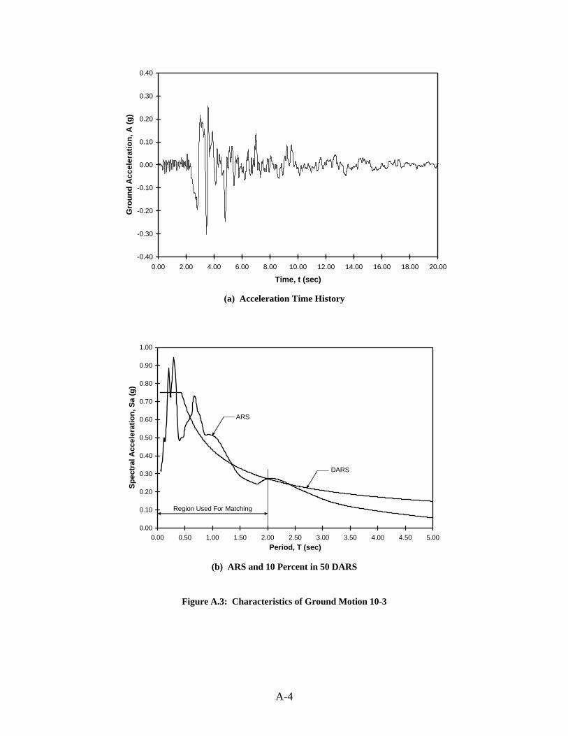
-0.40
-0.30
-0.20
-0.10
0.00
0.10
0.20
0.30
0.40
0.00 2.00 4.00 6.00 8.00 10.00 12.00 14.00 16.00 18.00 20.00
Time, t (sec)
Gro
und
Acc
eler
atio
n, A
(g)
(a) Acceleration Time History
0.00
0.10
0.20
0.30
0.40
0.50
0.60
0.70
0.80
0.90
1.00
0.00 0.50 1.00 1.50 2.00 2.50 3.00 3.50 4.00 4.50 5.00Period, T (sec)
Spec
tral
Acc
eler
atio
n, S
a (g
)
DARS
ARS
Region Used For Matching
(b) ARS and 10 Percent in 50 DARS
Figure A.3: Characteristics of Ground Motion 10-3
A-4
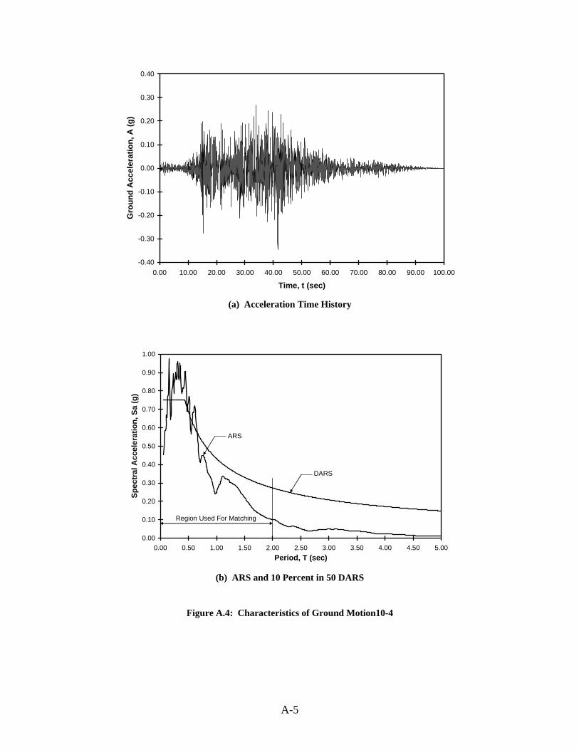
-0.40
-0.30
-0.20
-0.10
0.00
0.10
0.20
0.30
0.40
0.00 10.00 20.00 30.00 40.00 50.00 60.00 70.00 80.00 90.00 100.00
Time, t (sec)
Gro
und
Acc
eler
atio
n, A
(g)
(a) Acceleration Time History
0.00
0.10
0.20
0.30
0.40
0.50
0.60
0.70
0.80
0.90
1.00
0.00 0.50 1.00 1.50 2.00 2.50 3.00 3.50 4.00 4.50 5.00Period, T (sec)
Spec
tral
Acc
eler
atio
n, S
a (g
)
DARS
ARS
Region Used For Matching
(b) ARS and 10 Percent in 50 DARS
Figure A.4: Characteristics of Ground Motion10-4
A-5
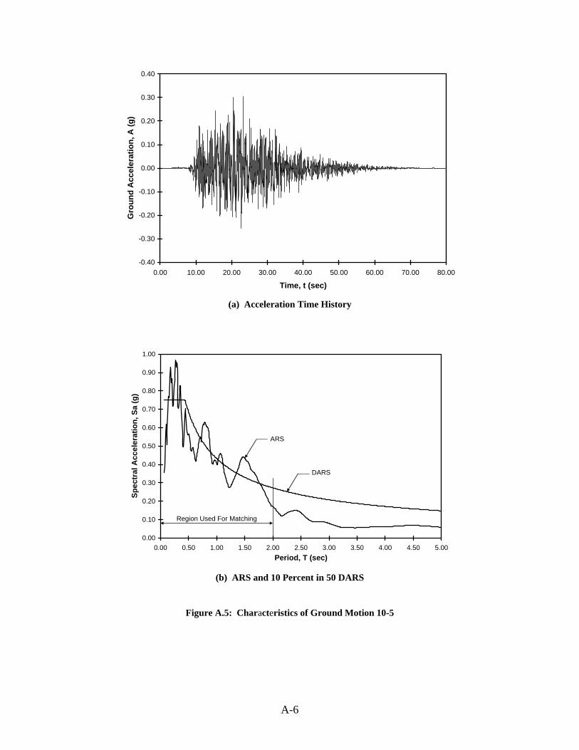
-0.40
-0.30
-0.20
-0.10
0.00
0.10
0.20
0.30
0.40
0.00 10.00 20.00 30.00 40.00 50.00 60.00 70.00 80.00
Time, t (sec)
Gro
und
Acc
eler
atio
n, A
(g)
(a) Acceleration Time History
0.00
0.10
0.20
0.30
0.40
0.50
0.60
0.70
0.80
0.90
1.00
0.00 0.50 1.00 1.50 2.00 2.50 3.00 3.50 4.00 4.50 5.00Period, T (sec)
Spec
tral
Acc
eler
atio
n, S
a (g
)
DARS
ARS
Region Used For Matching
(b) ARS and 10 Percent in 50 DARS
Figure A.5: Characteristics of Ground Motion 10-5
A-6
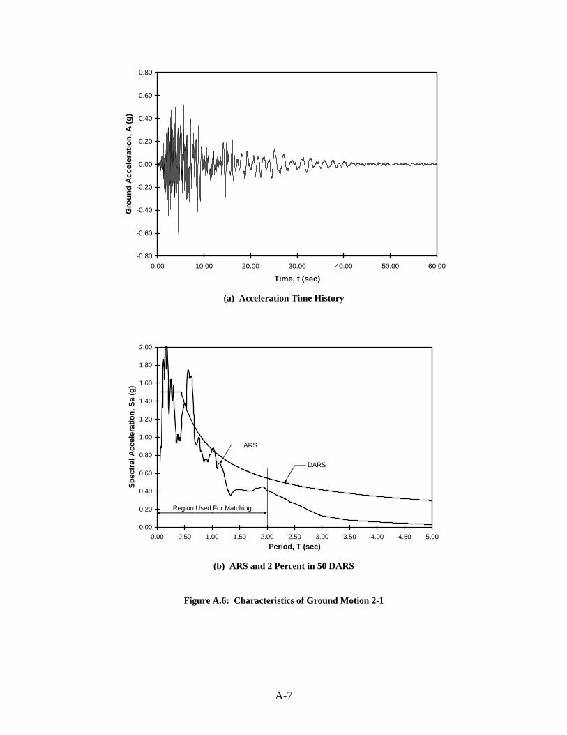
-0.80
-0.60
-0.40
-0.20
0.00
0.20
0.40
0.60
0.80
0.00 10.00 20.00 30.00 40.00 50.00 60.00
Time, t (sec)
Gro
und
Acc
eler
atio
n, A
(g)
(a) Acceleration Time History
0.00
0.20
0.40
0.60
0.80
1.00
1.20
1.40
1.60
1.80
2.00
0.00 0.50 1.00 1.50 2.00 2.50 3.00 3.50 4.00 4.50 5.00Period, T (sec)
Spec
tral
Acc
eler
atio
n, S
a (g
)
DARS
ARS
Region Used For Matching
(b) ARS and 2 Percent in 50 DARS
Figure A.6: Characteristics of Ground Motion 2-1
A-7
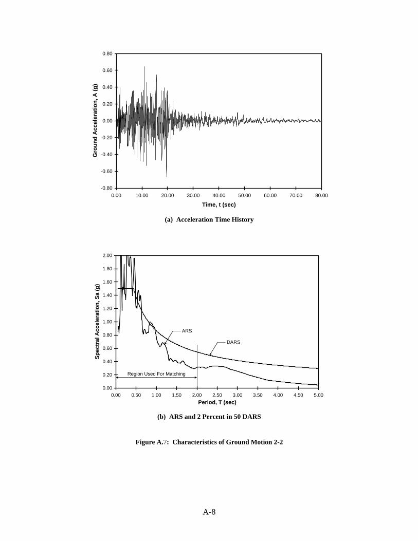
-0.80
-0.60
-0.40
-0.20
0.00
0.20
0.40
0.60
0.80
0.00 10.00 20.00 30.00 40.00 50.00 60.00 70.00 80.00
Time, t (sec)
Gro
und
Acc
eler
atio
n, A
(g)
(a) Acceleration Time History
0.00
0.20
0.40
0.60
0.80
1.00
1.20
1.40
1.60
1.80
2.00
0.00 0.50 1.00 1.50 2.00 2.50 3.00 3.50 4.00 4.50 5.00Period, T (sec)
Spec
tral
Acc
eler
atio
n, S
a (g
)
DARS
ARS
Region Used For Matching
(b) ARS and 2 Percent in 50 DARS
Figure A.7: Characteristics of Ground Motion 2-2
A-8
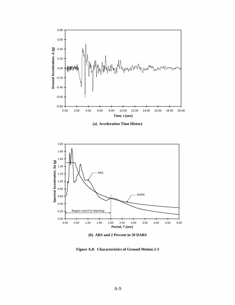
-0.80
-0.60
-0.40
-0.20
0.00
0.20
0.40
0.60
0.80
0.00 2.00 4.00 6.00 8.00 10.00 12.00 14.00 16.00 18.00 20.00
Time, t (sec)
Gro
und
Acc
eler
atio
n, A
(g)
(a) Acceleration Time History
0.00
0.20
0.40
0.60
0.80
1.00
1.20
1.40
1.60
1.80
2.00
0.00 0.50 1.00 1.50 2.00 2.50 3.00 3.50 4.00 4.50 5.00Period, T (sec)
Spec
tral
Acc
eler
atio
n, S
a (g
)
DARS
ARS
Region Used For Matching
(b) ARS and 2 Percent in 50 DARS
Figure A.8: Characteristics of Ground Motion 2-3
A-9

-0.80
-0.60
-0.40
-0.20
0.00
0.20
0.40
0.60
0.80
0.00 10.00 20.00 30.00 40.00 50.00 60.00 70.00 80.00 90.00 100.00
Time, t (sec)
Gro
und
Acc
eler
atio
n, A
(g)
(a) Acceleration Time History
0.00
0.20
0.40
0.60
0.80
1.00
1.20
1.40
1.60
1.80
2.00
0.00 0.50 1.00 1.50 2.00 2.50 3.00 3.50 4.00 4.50 5.00Period, T (sec)
Spec
tral
Acc
eler
atio
n, S
a (g
)
DARS
ARS
Region Used For Matching
(b) ARS and 2 Percent in 50 DARS
Figure A.9: Characteristics of Ground Motion 2-4
A-10
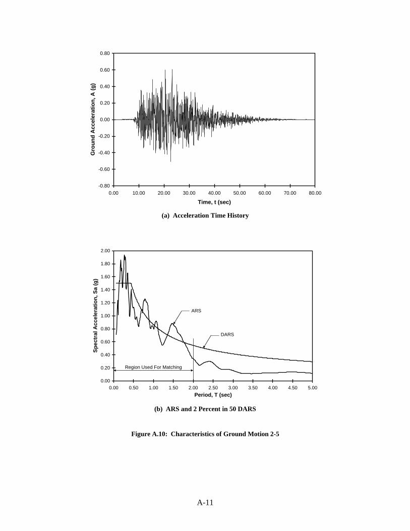
-0.80
-0.60
-0.40
-0.20
0.00
0.20
0.40
0.60
0.80
0.00 10.00 20.00 30.00 40.00 50.00 60.00 70.00 80.00
Time, t (sec)
Gro
und
Acc
eler
atio
n, A
(g)
(a) Acceleration Time History
0.00
0.20
0.40
0.60
0.80
1.00
1.20
1.40
1.60
1.80
2.00
0.00 0.50 1.00 1.50 2.00 2.50 3.00 3.50 4.00 4.50 5.00Period, T (sec)
Spec
tral
Acc
eler
atio
n, S
a (g
)
DARS
ARS
Region Used For Matching
(b) ARS and 2 Percent in 50 DARS
Figure A.10: Characteristics of Ground Motion 2-5
A-11

A-12
APPENDIX B RESULTS FROM EARTHQUAKE ANALYSES
OF REINFORCED CONCRETE FRAMES
Chapter 7 describes earthquake analyses of the reinforced concrete frames and
discusses the results from those analyses. The reinforced concrete frames were subjected
to the 10 ground motions described in Chapter 5 to establish maximum displacements
and residual displacements. The 10 ground motions contained five motions with a 10
percent probability of exceedance in 50 years (10 percent in 50) and five motions with a 2
percent probability of exceedance in 50 years (2 percent in 50). Chapter 7 contains only
the plots for response quantities resulting from the 2% in 50 ground motions. This
appendix contains the tables and plots that summarize the responses of the reinforced
concrete frames to the 10 percent in 50 ground motions. This appendix also includes the
tables that summarize the responses of the hybrid frames to the 2 percent in 50 ground
motions. Chapter 7 may be consulted for further information regarding the plots and
quantities presented in this appendix.
Throughout this appendix, the mean values shown in the tables and figures are the
average calculated from the five 10 percent in 50 ground motions. For the 2 percent in 50
ground motions, ten frame/ground motion combinations had a displacement of over 100
in., with OpenSees encountering convergence problems with each occurrence. For this
study, these values were omitted when the mean values were calculated for the 2 percent
in 50 ground motions. The combinations that encountered convergence problems are
shown in Table B.2 as DNC (Did Not Converge).
B-1
Table B.1: Maximum Displacements, 10 Percent in 50, Reinforced Concrete Frames
(in.) (%) (in.) (%) (in.) (%) (in.) (%) (in.) (%) (in.) (%)5.005.05 2.491 1.04 2.625 1.09 2.577 1.07 2.370 0.99 3.070 1.28 2.626 1.095.005.10 3.063 1.28 3.469 1.45 4.153 1.73 2.784 1.16 4.861 2.03 3.666 1.535.005.15 4.282 1.78 3.488 1.45 5.417 2.26 2.763 1.15 7.431 3.10 4.676 1.955.010.05 2.662 1.11 2.366 0.99 1.214 0.51 2.300 0.96 1.799 0.75 2.068 0.865.010.10 2.783 1.16 2.808 1.17 3.261 1.36 2.570 1.07 3.382 1.41 2.961 1.235.010.15 3.613 1.51 3.181 1.33 3.870 1.61 2.966 1.24 3.650 1.52 3.456 1.445.020.05 1.484 0.62 2.345 0.98 1.177 0.49 1.786 0.74 2.186 0.91 1.795 0.755.020.10 2.630 1.10 3.037 1.27 2.159 0.90 2.451 1.02 2.511 1.05 2.558 1.075.020.15 2.656 1.11 2.632 1.10 3.219 1.34 2.358 0.98 3.074 1.28 2.788 1.165.030.05 1.081 0.45 2.039 0.85 1.242 0.52 1.585 0.66 1.841 0.77 1.558 0.655.030.10 2.651 1.10 2.152 0.90 1.473 0.61 2.071 0.86 1.337 0.56 1.937 0.815.030.15 2.605 1.09 2.668 1.11 2.805 1.17 2.509 1.05 2.477 1.03 2.613 1.096.005.05 3.668 1.27 3.392 1.18 3.131 1.09 2.491 0.87 3.467 1.20 3.230 1.126.005.10 4.212 1.46 4.437 1.54 6.035 2.10 3.349 1.16 6.687 2.32 4.944 1.726.005.15 7.711 2.68 3.831 1.33 8.069 2.80 6.413 2.23 6.389 2.22 6.483 2.256.010.05 2.646 0.92 2.551 0.89 3.019 1.05 2.392 0.83 3.433 1.19 2.808 0.986.010.10 4.273 1.48 3.874 1.35 4.133 1.44 3.123 1.08 4.280 1.49 3.937 1.376.010.15 4.872 1.69 4.481 1.56 6.744 2.34 4.273 1.48 6.885 2.39 5.451 1.896.020.05 2.743 0.95 2.657 0.92 1.638 0.57 2.524 0.88 1.976 0.69 2.308 0.806.020.10 3.330 1.16 3.326 1.15 3.587 1.25 2.984 1.04 3.421 1.19 3.329 1.166.020.15 3.244 1.13 3.492 1.21 4.828 1.68 3.227 1.12 4.710 1.64 3.900 1.356.030.05 2.273 0.79 2.384 0.83 0.947 0.33 2.525 0.88 2.480 0.86 2.122 0.746.030.10 3.170 1.10 2.967 1.03 3.131 1.09 2.696 0.94 2.897 1.01 2.972 1.036.030.15 3.694 1.28 3.675 1.28 3.550 1.23 2.640 0.92 3.959 1.37 3.504 1.227.005.05 5.132 1.53 3.564 1.06 4.783 1.42 3.030 0.90 4.696 1.40 4.241 1.267.005.10 7.678 2.29 3.879 1.15 7.877 2.34 6.538 1.95 6.606 1.97 6.516 1.947.005.15 7.932 2.36 5.437 1.62 10.723 3.19 6.355 1.89 8.134 2.42 7.716 2.307.010.05 3.843 1.14 3.880 1.15 3.632 1.08 2.867 0.85 3.670 1.09 3.578 1.077.010.10 5.003 1.49 5.003 1.49 6.671 1.99 4.995 1.49 5.856 1.74 5.505 1.647.010.15 6.996 2.08 4.635 1.38 7.705 2.29 4.639 1.38 6.275 1.87 6.050 1.807.020.05 3.379 1.01 3.210 0.96 3.872 1.15 3.242 0.96 3.449 1.03 3.430 1.027.020.10 3.616 1.08 3.953 1.18 4.573 1.36 3.314 0.99 4.224 1.26 3.936 1.177.020.15 4.175 1.24 5.151 1.53 6.571 1.96 3.525 1.05 4.783 1.42 4.841 1.447.030.05 3.364 1.00 3.743 1.11 2.082 0.62 3.375 1.00 2.587 0.77 3.030 0.907.030.10 3.384 1.01 4.207 1.25 4.055 1.21 3.737 1.11 4.602 1.37 3.997 1.197.030.15 5.739 1.71 3.811 1.13 5.581 1.66 3.458 1.03 5.112 1.52 4.740 1.41
FrameΔmax
LcolΔmax
Ground Motion 10 - 1
Ground Motion 10 - 2
Ground Motion 10 - 3
ΔmaxΔmax
LcolΔmax
Δmax
LcolΔmax
Δmax
Lcol
Ground Motion 10 - 4
Ground Motion 10 - 5 Mean
Δmax
LcolΔmax
Δmax
LcolΔmax
B-2
Table B.2: Maximum Displacements, 2 Percent in 50, Reinforced Concrete Frames
(in.) (%) (in.) (%) (in.) (%) (in.) (%) (in.) (%) (in.) (%)5.005.05 5.668 2.36 5.965 2.49 10.205 4.25 3.702 1.54 7.185 2.99 6.545 2.735.005.10 10.281 4.28 7.693 3.21 DNC DNC 9.336 3.89 10.920 4.55 9.558 3.985.005.15 DNC DNC 9.393 3.91 DNC DNC 9.811 4.09 DNC DNC 9.602 4.005.010.05 4.123 1.72 4.237 1.77 5.108 2.13 3.679 1.53 4.310 1.80 4.291 1.795.010.10 6.723 2.80 5.991 2.50 11.777 4.91 3.935 1.64 7.372 3.07 7.159 2.985.010.15 6.496 2.71 6.626 2.76 DNC DNC 8.489 3.54 8.997 3.75 7.652 3.195.020.05 2.819 1.17 3.236 1.35 1.996 0.83 2.727 1.14 3.004 1.25 2.756 1.155.020.10 4.556 1.90 4.422 1.84 6.212 2.59 4.007 1.67 5.438 2.27 4.927 2.055.020.15 5.697 2.37 5.596 2.33 11.305 4.71 3.815 1.59 6.848 2.85 6.652 2.775.030.05 1.899 0.79 3.151 1.31 2.019 0.84 2.186 0.91 2.039 0.85 2.259 0.945.030.10 4.345 1.81 4.215 1.76 3.985 1.66 3.635 1.51 3.739 1.56 3.984 1.665.030.15 5.090 2.12 5.090 2.12 8.313 3.46 3.601 1.50 5.892 2.46 5.597 2.336.005.05 6.435 2.23 5.647 1.96 12.829 4.45 4.646 1.61 10.541 3.66 8.020 2.786.005.10 11.342 3.94 9.987 3.47 DNC DNC 8.907 3.09 13.426 4.66 10.916 3.796.005.15 11.500 3.99 16.021 5.56 DNC DNC 6.696 2.33 12.333 4.28 11.637 4.046.010.05 5.581 1.94 5.407 1.88 9.365 3.25 4.019 1.40 6.412 2.23 6.157 2.146.010.10 6.638 2.31 7.568 2.63 15.605 5.42 8.290 2.88 8.564 2.97 9.333 3.246.010.15 13.208 4.59 9.754 3.39 DNC DNC 7.382 2.56 10.972 3.81 10.329 3.596.020.05 4.118 1.43 4.384 1.52 4.189 1.45 3.705 1.29 3.993 1.39 4.078 1.426.020.10 5.204 1.81 5.364 1.86 10.686 3.71 4.092 1.42 7.122 2.47 6.494 2.256.020.15 6.274 2.18 6.842 2.38 14.457 5.02 6.573 2.28 11.269 3.91 9.083 3.156.030.05 4.217 1.46 3.725 1.29 2.921 1.01 3.474 1.21 3.563 1.24 3.580 1.246.030.10 5.143 1.79 5.368 1.86 7.186 2.50 3.892 1.35 6.064 2.11 5.531 1.926.030.15 6.755 2.35 5.254 1.82 12.425 4.31 4.445 1.54 7.051 2.45 7.186 2.507.005.05 11.207 3.34 7.738 2.30 18.212 5.42 8.682 2.58 9.756 2.90 11.119 3.317.005.10 11.657 3.47 16.067 4.78 28.443 8.47 7.041 2.10 11.551 3.44 14.952 4.457.005.15 12.741 3.79 16.979 5.05 DNC DNC 8.908 2.65 12.517 3.73 12.786 3.817.010.05 7.337 2.18 5.493 1.63 12.155 3.62 4.947 1.47 7.551 2.25 7.497 2.237.010.10 12.158 3.62 9.380 2.79 18.736 5.58 7.994 2.38 9.781 2.91 11.610 3.467.010.15 11.041 3.29 11.642 3.46 DNC DNC 8.188 2.44 12.367 3.68 10.810 3.227.020.05 5.188 1.54 5.264 1.57 6.210 1.85 4.719 1.40 5.808 1.73 5.438 1.627.020.10 6.777 2.02 6.828 2.03 12.662 3.77 5.012 1.49 7.814 2.33 7.819 2.337.020.15 11.351 3.38 8.327 2.48 16.922 5.04 8.190 2.44 8.942 2.66 10.746 3.207.030.05 4.413 1.31 4.813 1.43 5.100 1.52 4.266 1.27 4.511 1.34 4.621 1.387.030.10 7.330 2.18 5.449 1.62 12.100 3.60 4.954 1.47 7.516 2.24 7.470 2.227.030.15 7.268 2.16 7.778 2.31 13.063 3.89 5.119 1.52 11.248 3.35 8.895 2.65
Note: DNC indicates earthquake analysis did not converge
FrameΔmax
LcolΔmax
Ground Motion 2 - 1
Ground Motion 2 - 2
Ground Motion 2 - 3
ΔmaxΔmax
LcolΔmax
Δmax
LcolΔmax
Δmax
Lcol
Ground Motion 2 - 4
Ground Motion 2 - 5 Mean
Δmax
LcolΔmax
Δmax
LcolΔmax
B-3
0 0.5 1 1.5 2 2.5 3 3.50
0.5
1
1.5
2
2.5
3
(a) ρ (%)
Δm
ax/L
col (%
)
Mean
0 0.5 1 1.5 2 2.5 3 3.50
0.5
1
1.5
2
2.5
3
(c) ρ (%)
Δm
ax/L
col (%
)
0 0.5 1 1.5 2 2.5 3 3.50
0.5
1
1.5
2
2.5
3
(e) ρ (%)
Δm
ax/L
col (%
)
0 0.5 1 1.5 2 2.5 3 3.50
0.5
1
1.5
2
2.5
3
(b) ρ (%)
Δm
ax/L
col (%
)
Mean + 1 Standard Deviation
Pcol/fcAg = 0.05Pcol/fcAg = 0.10Pcol/fcAg = 0.15
0 0.5 1 1.5 2 2.5 3 3.50
0.5
1
1.5
2
2.5
3
(d) ρ (%)
Δm
ax/L
col (%
)
0 0.5 1 1.5 2 2.5 3 3.50
0.5
1
1.5
2
2.5
3
(f) ρ (%)
Δm
ax/L
col (%
)
Figure B.1: Trends in Drift Ratio, 10 Percent in 50, Reinforced Concrete Frames (a) and (b) 5col colL D = , (c) and (d) 6col colL D = , and (e) and (f) 7col colL D =
B-4
0 20 40 60 80 100 1200
0.5
1
1.5
2
2.5
3
Fcon004/Ptotal (%)
Mea
n Δ
max
/Lco
l (%)
ρ = 0.5%ρ = 1.0%ρ = 2.0%ρ = 3.0%
Figure B.2: Effect of Strength on Mean Drift Ratio, 10 Percent in 50, Reinforced Concrete Frames
0 20 40 60 80 100 1200
0.5
1
1.5
2
2.5
3
Fcon004/Ptotal (%)
Mea
n +
1 S
td D
evia
tion
Δ max
/Lco
l (%)
Pcol/fcAg = 0.05Pcol/fcAg = 0.10Pcol/fcAg = 0.15
Figure B.3: Effect of Strength on Mean Plus One Standard Deviation Drift Ratio, 10 Percent in 50, Reinforced Concrete Frames
B-5
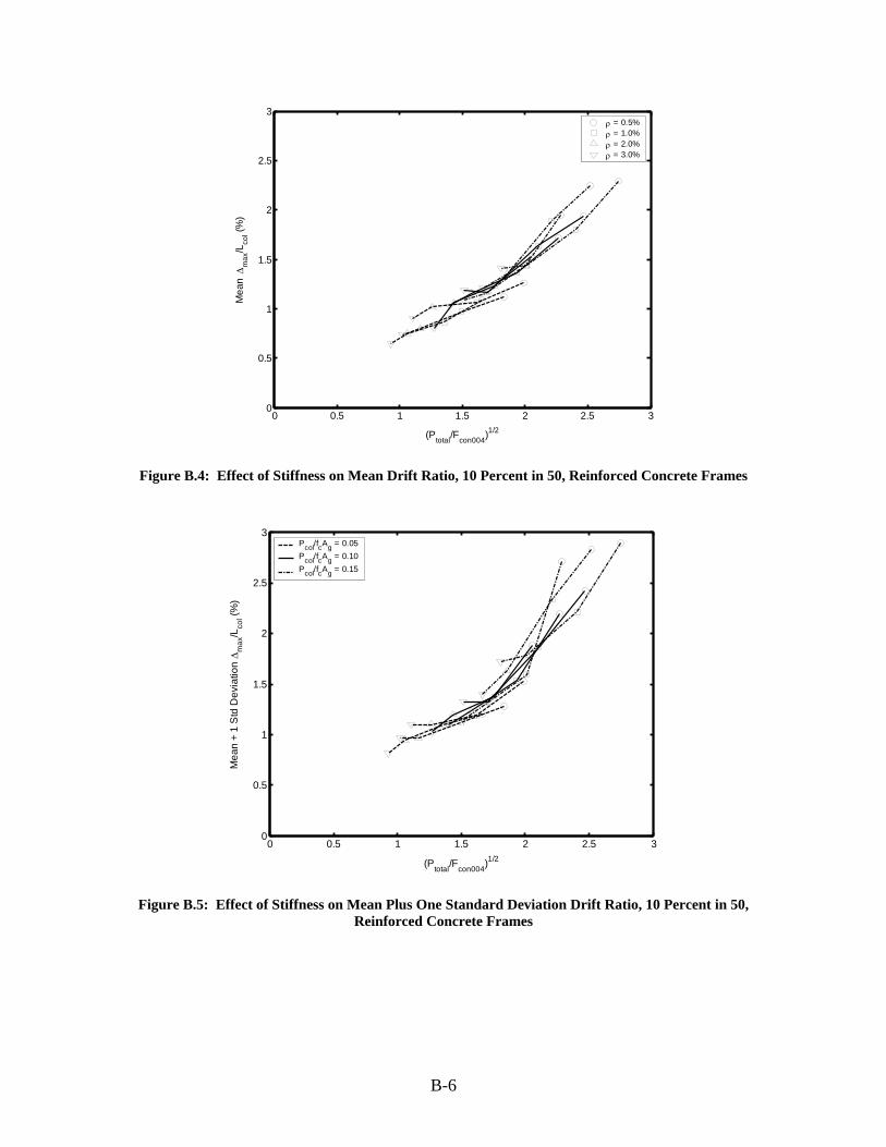
0 0.5 1 1.5 2 2.5 30
0.5
1
1.5
2
2.5
3
(Ptotal/Fcon004)1/2
Mea
n Δ
max
/Lco
l (%)
ρ = 0.5%ρ = 1.0%ρ = 2.0%ρ = 3.0%
Figure B.4: Effect of Stiffness on Mean Drift Ratio, 10 Percent in 50, Reinforced Concrete Frames
0 0.5 1 1.5 2 2.5 30
0.5
1
1.5
2
2.5
3
(Ptotal/Fcon004)1/2
Mea
n +
1 S
td D
evia
tion
Δm
ax/L
col (%
)
Pcol/fcAg = 0.05Pcol/fcAg = 0.10Pcol/fcAg = 0.15
Figure B.5: Effect of Stiffness on Mean Plus One Standard Deviation Drift Ratio, 10 Percent in 50, Reinforced Concrete Frames
B-6
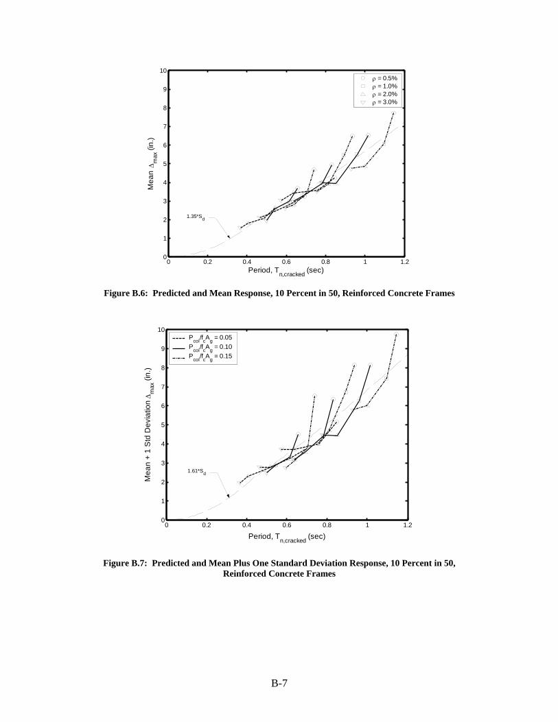
0 0.2 0.4 0.6 0.8 1 1.20
1
2
3
4
5
6
7
8
9
10
Period, Tn,cracked (sec)
Mea
n Δ
max
(in.
)
ρ = 0.5%ρ = 1.0%ρ = 2.0%ρ = 3.0%
1.35*Sd
Figure B.6: Predicted and Mean Response, 10 Percent in 50, Reinforced Concrete Frames
0 0.2 0.4 0.6 0.8 1 1.20
1
2
3
4
5
6
7
8
9
10
Period, Tn,cracked (sec)
Mea
n +
1 S
td D
evia
tion
Δ max
(in.
)
Pcol/fcAg = 0.05Pcol/fcAg = 0.10Pcol/fcAg = 0.15
1.61*Sd
Figure B.7: Predicted and Mean Plus One Standard Deviation Response, 10 Percent in 50, Reinforced Concrete Frames
B-7

B-8
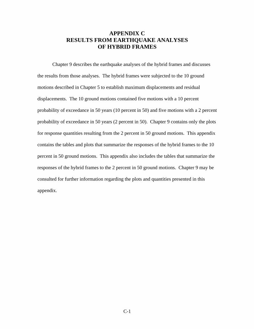
APPENDIX C RESULTS FROM EARTHQUAKE ANALYSES
OF HYBRID FRAMES
Chapter 9 describes the earthquake analyses of the hybrid frames and discusses
the results from those analyses. The hybrid frames were subjected to the 10 ground
motions described in Chapter 5 to establish maximum displacements and residual
displacements. The 10 ground motions contained five motions with a 10 percent
probability of exceedance in 50 years (10 percent in 50) and five motions with a 2 percent
probability of exceedance in 50 years (2 percent in 50). Chapter 9 contains only the plots
for response quantities resulting from the 2 percent in 50 ground motions. This appendix
contains the tables and plots that summarize the responses of the hybrid frames to the 10
percent in 50 ground motions. This appendix also includes the tables that summarize the
responses of the hybrid frames to the 2 percent in 50 ground motions. Chapter 9 may be
consulted for further information regarding the plots and quantities presented in this
appendix.
C-1
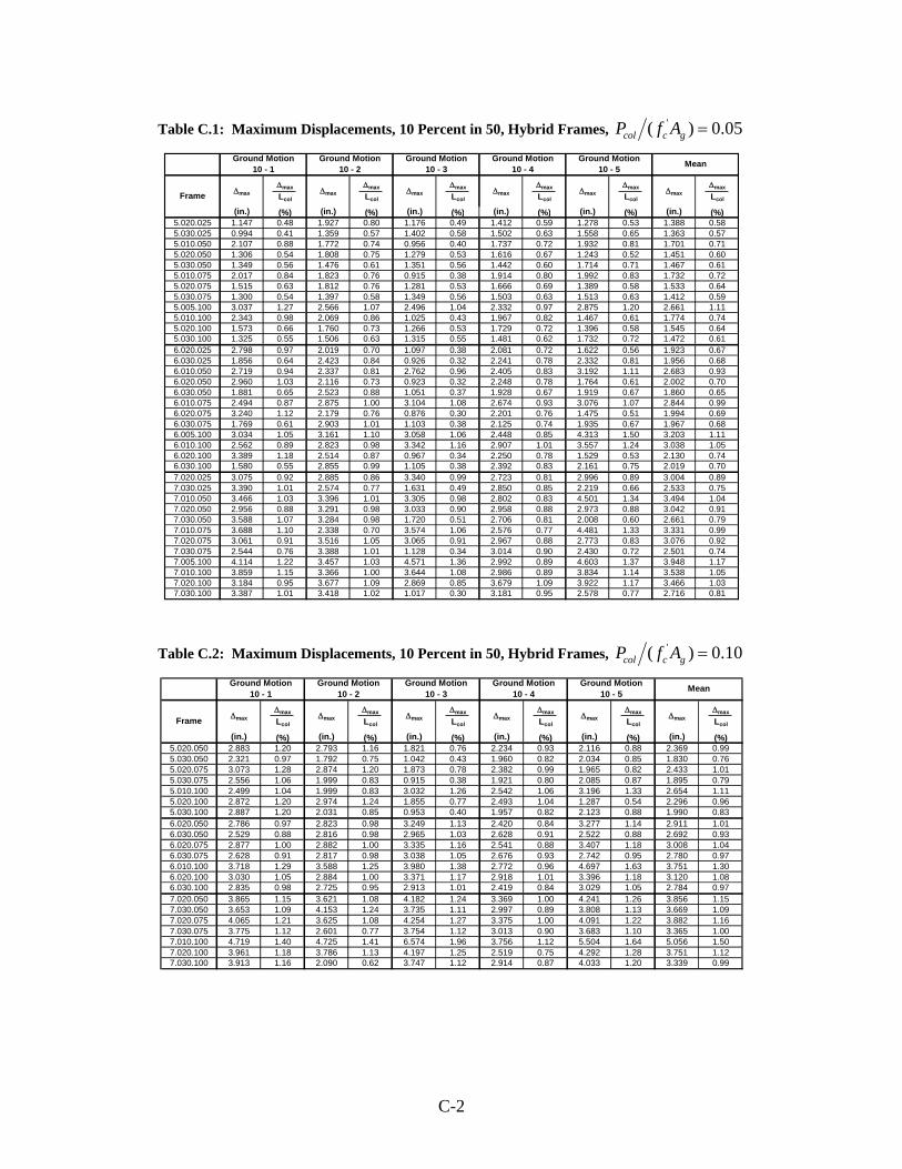
Table C.1: Maximum Displacements, 10 Percent in 50, Hybrid Frames, '( ) 0.05col c gP f A =
(in.) (%) (in.) (%) (in.) (%) (in.) (%) (in.) (%) (in.) (%)5.020.025 1.147 0.48 1.927 0.80 1.176 0.49 1.412 0.59 1.278 0.53 1.388 0.585.030.025 0.994 0.41 1.359 0.57 1.402 0.58 1.502 0.63 1.558 0.65 1.363 0.575.010.050 2.107 0.88 1.772 0.74 0.956 0.40 1.737 0.72 1.932 0.81 1.701 0.715.020.050 1.306 0.54 1.808 0.75 1.279 0.53 1.616 0.67 1.243 0.52 1.451 0.605.030.050 1.349 0.56 1.476 0.61 1.351 0.56 1.442 0.60 1.714 0.71 1.467 0.615.010.075 2.017 0.84 1.823 0.76 0.915 0.38 1.914 0.80 1.992 0.83 1.732 0.725.020.075 1.515 0.63 1.812 0.76 1.281 0.53 1.666 0.69 1.389 0.58 1.533 0.645.030.075 1.300 0.54 1.397 0.58 1.349 0.56 1.503 0.63 1.513 0.63 1.412 0.595.005.100 3.037 1.27 2.566 1.07 2.496 1.04 2.332 0.97 2.875 1.20 2.661 1.115.010.100 2.343 0.98 2.069 0.86 1.025 0.43 1.967 0.82 1.467 0.61 1.774 0.745.020.100 1.573 0.66 1.760 0.73 1.266 0.53 1.729 0.72 1.396 0.58 1.545 0.645.030.100 1.325 0.55 1.506 0.63 1.315 0.55 1.481 0.62 1.732 0.72 1.472 0.616.020.025 2.798 0.97 2.019 0.70 1.097 0.38 2.081 0.72 1.622 0.56 1.923 0.676.030.025 1.856 0.64 2.423 0.84 0.926 0.32 2.241 0.78 2.332 0.81 1.956 0.686.010.050 2.719 0.94 2.337 0.81 2.762 0.96 2.405 0.83 3.192 1.11 2.683 0.936.020.050 2.960 1.03 2.116 0.73 0.923 0.32 2.248 0.78 1.764 0.61 2.002 0.706.030.050 1.881 0.65 2.523 0.88 1.051 0.37 1.928 0.67 1.919 0.67 1.860 0.656.010.075 2.494 0.87 2.875 1.00 3.104 1.08 2.674 0.93 3.076 1.07 2.844 0.996.020.075 3.240 1.12 2.179 0.76 0.876 0.30 2.201 0.76 1.475 0.51 1.994 0.696.030.075 1.769 0.61 2.903 1.01 1.103 0.38 2.125 0.74 1.935 0.67 1.967 0.686.005.100 3.034 1.05 3.161 1.10 3.058 1.06 2.448 0.85 4.313 1.50 3.203 1.116.010.100 2.562 0.89 2.823 0.98 3.342 1.16 2.907 1.01 3.557 1.24 3.038 1.056.020.100 3.389 1.18 2.514 0.87 0.967 0.34 2.250 0.78 1.529 0.53 2.130 0.746.030.100 1.580 0.55 2.855 0.99 1.105 0.38 2.392 0.83 2.161 0.75 2.019 0.707.020.025 3.075 0.92 2.885 0.86 3.340 0.99 2.723 0.81 2.996 0.89 3.004 0.897.030.025 3.390 1.01 2.574 0.77 1.631 0.49 2.850 0.85 2.219 0.66 2.533 0.757.010.050 3.466 1.03 3.396 1.01 3.305 0.98 2.802 0.83 4.501 1.34 3.494 1.047.020.050 2.956 0.88 3.291 0.98 3.033 0.90 2.958 0.88 2.973 0.88 3.042 0.917.030.050 3.588 1.07 3.284 0.98 1.720 0.51 2.706 0.81 2.008 0.60 2.661 0.797.010.075 3.688 1.10 2.338 0.70 3.574 1.06 2.576 0.77 4.481 1.33 3.331 0.997.020.075 3.061 0.91 3.516 1.05 3.065 0.91 2.967 0.88 2.773 0.83 3.076 0.927.030.075 2.544 0.76 3.388 1.01 1.128 0.34 3.014 0.90 2.430 0.72 2.501 0.747.005.100 4.114 1.22 3.457 1.03 4.571 1.36 2.992 0.89 4.603 1.37 3.948 1.177.010.100 3.859 1.15 3.366 1.00 3.644 1.08 2.986 0.89 3.834 1.14 3.538 1.057.020.100 3.184 0.95 3.677 1.09 2.869 0.85 3.679 1.09 3.922 1.17 3.466 1.037.030.100 3.387 1.01 3.418 1.02 1.017 0.30 3.181 0.95 2.578 0.77 2.716 0.81
Δmax
LcolΔmax
Δmax
LcolΔmax
Δmax
LcolΔmax
Δmax
Lcol
Ground Motion 10 - 4
Ground Motion 10 - 5 Mean
FrameΔmax
LcolΔmax
Ground Motion 10 - 1
Ground Motion 10 - 2
Ground Motion 10 - 3
ΔmaxΔmax
LcolΔmax
Table C.2: Maximum Displacements, 10 Percent in 50, Hybrid Frames, '( ) 0.10col c gP f A =
(in.) (%) (in.) (%) (in.) (%) (in.) (%) (in.) (%) (in.) (%)5.020.050 2.883 1.20 2.793 1.16 1.821 0.76 2.234 0.93 2.116 0.88 2.369 0.995.030.050 2.321 0.97 1.792 0.75 1.042 0.43 1.960 0.82 2.034 0.85 1.830 0.765.020.075 3.073 1.28 2.874 1.20 1.873 0.78 2.382 0.99 1.965 0.82 2.433 1.015.030.075 2.556 1.06 1.999 0.83 0.915 0.38 1.921 0.80 2.085 0.87 1.895 0.795.010.100 2.499 1.04 1.999 0.83 3.032 1.26 2.542 1.06 3.196 1.33 2.654 1.115.020.100 2.872 1.20 2.974 1.24 1.855 0.77 2.493 1.04 1.287 0.54 2.296 0.965.030.100 2.887 1.20 2.031 0.85 0.953 0.40 1.957 0.82 2.123 0.88 1.990 0.836.020.050 2.786 0.97 2.823 0.98 3.249 1.13 2.420 0.84 3.277 1.14 2.911 1.016.030.050 2.529 0.88 2.816 0.98 2.965 1.03 2.628 0.91 2.522 0.88 2.692 0.936.020.075 2.877 1.00 2.882 1.00 3.335 1.16 2.541 0.88 3.407 1.18 3.008 1.046.030.075 2.628 0.91 2.817 0.98 3.038 1.05 2.676 0.93 2.742 0.95 2.780 0.976.010.100 3.718 1.29 3.588 1.25 3.980 1.38 2.772 0.96 4.697 1.63 3.751 1.306.020.100 3.030 1.05 2.884 1.00 3.371 1.17 2.918 1.01 3.396 1.18 3.120 1.086.030.100 2.835 0.98 2.725 0.95 2.913 1.01 2.419 0.84 3.029 1.05 2.784 0.977.020.050 3.865 1.15 3.621 1.08 4.182 1.24 3.369 1.00 4.241 1.26 3.856 1.157.030.050 3.653 1.09 4.153 1.24 3.735 1.11 2.997 0.89 3.808 1.13 3.669 1.097.020.075 4.065 1.21 3.625 1.08 4.254 1.27 3.375 1.00 4.091 1.22 3.882 1.167.030.075 3.775 1.12 2.601 0.77 3.754 1.12 3.013 0.90 3.683 1.10 3.365 1.007.010.100 4.719 1.40 4.725 1.41 6.574 1.96 3.756 1.12 5.504 1.64 5.056 1.507.020.100 3.961 1.18 3.786 1.13 4.197 1.25 2.519 0.75 4.292 1.28 3.751 1.127.030.100 3.913 1.16 2.090 0.62 3.747 1.12 2.914 0.87 4.033 1.20 3.339 0.99
FrameΔmax
LcolΔmax
Ground Motion 10 - 1
Ground Motion 10 - 2
Ground Motion 10 - 3
ΔmaxΔmax
LcolΔmax
Δmax
LcolΔmax
Δmax
Lcol
Ground Motion 10 - 4
Ground Motion 10 - 5 Mean
Δmax
LcolΔmax
Δmax
LcolΔmax
C-2
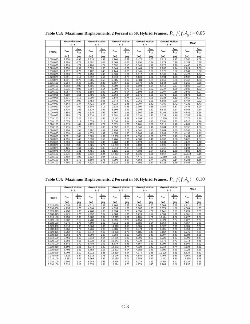
Table C.3: Maximum Displacements, 2 Percent in 50, Hybrid Frames, '( ) 0.05col c gP f A =
(in.) (%) (in.) (%) (in.) (%) (in.) (%) (in.) (%) (in.) (%)5.020.025 2.356 0.98 3.318 1.38 1.960 0.82 2.472 1.03 2.818 1.17 2.585 1.085.030.025 1.726 0.72 2.602 1.08 2.065 0.86 2.250 0.94 1.874 0.78 2.104 0.885.010.050 4.259 1.77 4.100 1.71 5.052 2.10 3.546 1.48 5.272 2.20 4.446 1.855.020.050 2.200 0.92 3.599 1.50 1.844 0.77 2.444 1.02 2.982 1.24 2.614 1.095.030.050 1.757 0.73 3.482 1.45 2.144 0.89 2.345 0.98 1.976 0.82 2.341 0.985.010.075 4.283 1.78 4.750 1.98 4.339 1.81 3.617 1.51 5.145 2.14 4.427 1.845.020.075 2.681 1.12 3.812 1.59 1.810 0.75 3.169 1.32 3.194 1.33 2.933 1.225.030.075 1.901 0.79 3.785 1.58 2.205 0.92 2.384 0.99 2.059 0.86 2.467 1.035.005.100 5.954 2.48 5.805 2.42 9.567 3.99 3.579 1.49 6.844 2.85 6.350 2.655.010.100 4.853 2.02 4.805 2.00 4.709 1.96 3.694 1.54 6.418 2.67 4.896 2.045.020.100 2.235 0.93 3.684 1.54 1.790 0.75 3.641 1.52 3.327 1.39 2.936 1.225.030.100 1.957 0.82 3.893 1.62 2.256 0.94 2.596 1.08 2.107 0.88 2.562 1.076.020.025 4.360 1.51 3.706 1.29 3.863 1.34 3.675 1.28 3.773 1.31 3.875 1.356.030.025 3.301 1.15 3.000 1.04 2.140 0.74 2.917 1.01 3.234 1.12 2.919 1.016.010.050 5.748 2.00 5.782 2.01 9.843 3.42 3.761 1.31 6.888 2.39 6.404 2.226.020.050 4.143 1.44 4.421 1.54 4.218 1.46 3.797 1.32 4.080 1.42 4.132 1.436.030.050 4.606 1.60 3.349 1.16 2.528 0.88 3.390 1.18 3.369 1.17 3.448 1.206.010.075 5.426 1.88 5.539 1.92 8.609 2.99 3.799 1.32 6.832 2.37 6.041 2.106.020.075 4.354 1.51 4.516 1.57 4.767 1.66 3.907 1.36 5.164 1.79 4.542 1.586.030.075 4.985 1.73 3.630 1.26 2.651 0.92 3.534 1.23 3.739 1.30 3.708 1.296.005.100 6.513 2.26 5.321 1.85 12.143 4.22 4.394 1.53 10.508 3.65 7.776 2.706.010.100 6.075 2.11 6.079 2.11 9.030 3.14 4.105 1.43 7.291 2.53 6.516 2.266.020.100 4.715 1.64 4.925 1.71 5.071 1.76 3.981 1.38 5.711 1.98 4.881 1.696.030.100 5.115 1.78 3.971 1.38 2.557 0.89 3.346 1.16 3.784 1.31 3.755 1.307.020.025 5.194 1.55 5.282 1.57 6.798 2.02 4.361 1.30 5.204 1.55 5.368 1.607.030.025 4.836 1.44 4.673 1.39 4.355 1.30 3.963 1.18 2.869 0.85 4.139 1.237.010.050 7.001 2.08 5.665 1.69 12.086 3.60 4.350 1.29 8.370 2.49 7.494 2.237.020.050 4.796 1.43 5.330 1.59 6.766 2.01 4.908 1.46 6.307 1.88 5.622 1.677.030.050 4.593 1.37 4.539 1.35 4.788 1.43 4.174 1.24 5.034 1.50 4.626 1.387.010.075 6.898 2.05 5.925 1.76 11.283 3.36 4.138 1.23 7.895 2.35 7.228 2.157.020.075 5.425 1.61 6.225 1.85 7.214 2.15 4.844 1.44 7.762 2.31 6.294 1.877.030.075 4.742 1.41 4.451 1.32 5.125 1.53 4.503 1.34 5.655 1.68 4.895 1.467.005.100 9.575 2.85 7.516 2.24 17.283 5.14 8.931 2.66 9.557 2.84 10.573 3.157.010.100 6.480 1.93 6.532 1.94 11.527 3.43 4.475 1.33 10.650 3.17 7.933 2.367.020.100 5.787 1.72 5.890 1.75 7.296 2.17 4.853 1.44 7.201 2.14 6.206 1.857.030.100 4.786 1.42 4.524 1.35 5.228 1.56 4.602 1.37 6.024 1.79 5.033 1.50
Δmax
LcolΔmax
Δmax
LcolΔmax
Δmax
LcolΔmax
Δmax
Lcol
Ground Motion 2 - 4
Ground Motion 2 - 5 Mean
FrameΔmax
LcolΔmax
Ground Motion 2 - 1
Ground Motion 2 - 2
Ground Motion 2 - 3
ΔmaxΔmax
LcolΔmax
Table C.4: Maximum Displacements, 2 Percent in 50, Hybrid Frames, '( ) 0.10col c gP f A =
(in.) (%) (in.) (%) (in.) (%) (in.) (%) (in.) (%) (in.) (%)5.020.050 4.538 1.89 4.511 1.88 6.164 2.57 3.840 1.60 5.505 2.29 4.911 2.055.030.050 4.235 1.76 4.694 1.96 4.035 1.68 3.607 1.50 3.873 1.61 4.089 1.705.020.075 4.750 1.98 4.760 1.98 6.634 2.76 4.096 1.71 6.141 2.56 5.276 2.205.030.075 4.221 1.76 4.897 2.04 4.384 1.83 3.774 1.57 4.530 1.89 4.361 1.825.010.100 6.959 2.90 5.682 2.37 12.015 5.01 4.105 1.71 10.124 4.22 7.777 3.245.020.100 5.037 2.10 4.730 1.97 6.691 2.79 4.150 1.73 6.529 2.72 5.427 2.265.030.100 4.276 1.78 4.599 1.92 4.711 1.96 3.686 1.54 5.564 2.32 4.567 1.906.020.050 5.418 1.88 5.463 1.90 10.319 3.58 4.006 1.39 6.822 2.37 6.406 2.226.030.050 5.066 1.76 5.266 1.83 7.586 2.63 3.873 1.34 6.501 2.26 5.659 1.966.020.075 5.762 2.00 5.942 2.06 10.828 3.76 4.186 1.45 7.162 2.49 6.776 2.356.030.075 5.063 1.76 5.394 1.87 7.760 2.69 4.286 1.49 6.997 2.43 5.900 2.056.010.100 7.461 2.59 7.318 2.54 17.075 5.93 8.901 3.09 9.226 3.20 9.996 3.476.020.100 5.983 2.08 6.232 2.16 10.943 3.80 4.330 1.50 7.876 2.73 7.073 2.466.030.100 5.542 1.92 5.489 1.91 8.139 2.83 4.357 1.51 6.990 2.43 6.104 2.127.020.050 6.598 1.96 6.048 1.80 12.572 3.74 4.720 1.40 9.210 2.74 7.830 2.337.030.050 6.403 1.91 5.658 1.68 11.893 3.54 4.582 1.36 7.605 2.26 7.228 2.157.020.075 6.708 2.00 8.012 2.38 13.230 3.94 4.974 1.48 11.125 3.31 8.810 2.627.030.075 7.620 2.27 5.918 1.76 12.176 3.62 4.840 1.44 7.765 2.31 7.664 2.287.010.100 12.983 3.86 9.569 2.85 20.180 6.01 7.953 2.37 11.113 3.31 12.360 3.687.020.100 7.192 2.14 8.245 2.45 13.616 4.05 5.075 1.51 10.419 3.10 8.910 2.657.030.100 7.324 2.18 6.078 1.81 12.624 3.76 4.873 1.45 8.785 2.61 7.937 2.36
FrameΔmax
LcolΔmax
Ground Motion 2 - 1
Ground Motion 2 - 2
Ground Motion 2 - 3
ΔmaxΔmax
LcolΔmax
Δmax
LcolΔmax
Δmax
Lcol
Ground Motion 2 - 4
Ground Motion 2 - 5 Mean
Δmax
LcolΔmax
Δmax
LcolΔmax
C-3
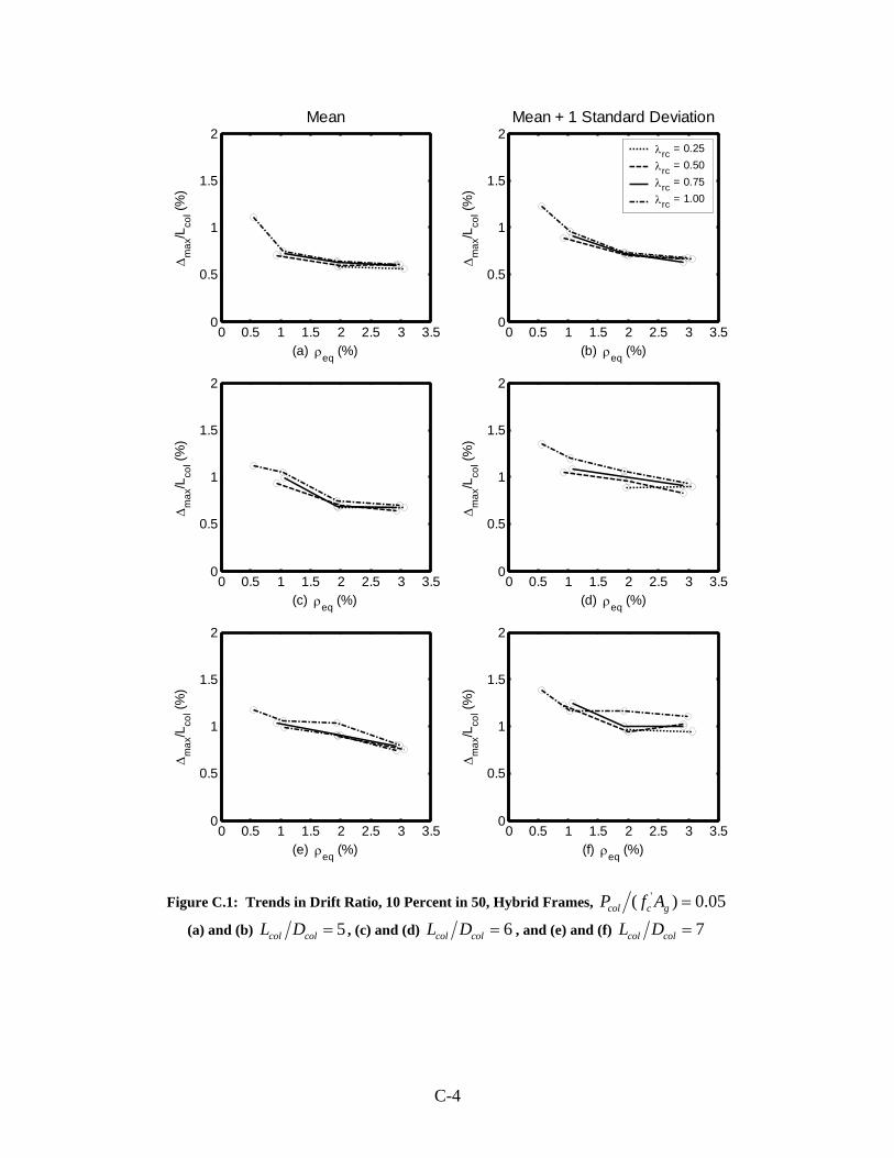
0 0.5 1 1.5 2 2.5 3 3.50
0.5
1
1.5
2
(a) ρeq (%)
Δm
ax/L
col (%
)
Mean
0 0.5 1 1.5 2 2.5 3 3.50
0.5
1
1.5
2
(c) ρeq (%)
Δm
ax/L
col (%
)
0 0.5 1 1.5 2 2.5 3 3.50
0.5
1
1.5
2
(e) ρeq (%)
Δm
ax/L
col (%
)
0 0.5 1 1.5 2 2.5 3 3.50
0.5
1
1.5
2
(b) ρeq (%)
Δm
ax/L
col (%
)
Mean + 1 Standard Deviation
λrc = 0.25λrc = 0.50λrc = 0.75λrc = 1.00
0 0.5 1 1.5 2 2.5 3 3.50
0.5
1
1.5
2
(d) ρeq (%)
Δm
ax/L
col (%
)
0 0.5 1 1.5 2 2.5 3 3.50
0.5
1
1.5
2
(f) ρeq (%)
Δm
ax/L
col (%
)
Figure C.1: Trends in Drift Ratio, 10 Percent in 50, Hybrid Frames, '( ) 0.05col c gP f A =
(a) and (b) 5col colL D = , (c) and (d) 6col colL D = , and (e) and (f) 7col colL D =
C-4
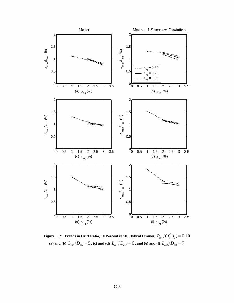
0 0.5 1 1.5 2 2.5 3 3.50
0.5
1
1.5
2
(a) ρeq (%)
Δm
ax/L
col (%
)
Mean
0 0.5 1 1.5 2 2.5 3 3.50
0.5
1
1.5
2
(c) ρeq (%)
Δm
ax/L
col (%
)
0 0.5 1 1.5 2 2.5 3 3.50
0.5
1
1.5
2
(e) ρeq (%)
Δm
ax/L
col (%
)
0 0.5 1 1.5 2 2.5 3 3.50
0.5
1
1.5
2
(b) ρeq (%)
Δm
ax/L
col (%
)
Mean + 1 Standard Deviation
λrc = 0.50λrc = 0.75λrc = 1.00
0 0.5 1 1.5 2 2.5 3 3.50
0.5
1
1.5
2
(d) ρeq (%)
Δm
ax/L
col (%
)
0 0.5 1 1.5 2 2.5 3 3.50
0.5
1
1.5
2
(f) ρeq (%)
Δm
ax/L
col (%
)
Figure C.2: Trends in Drift Ratio, 10 Percent in 50, Hybrid Frames, '( ) 0.10col c gP f A =
(a) and (b) 5col colL D = , (c) and (d) 6col colL D = , and (e) and (f) 7col colL D =
C-5
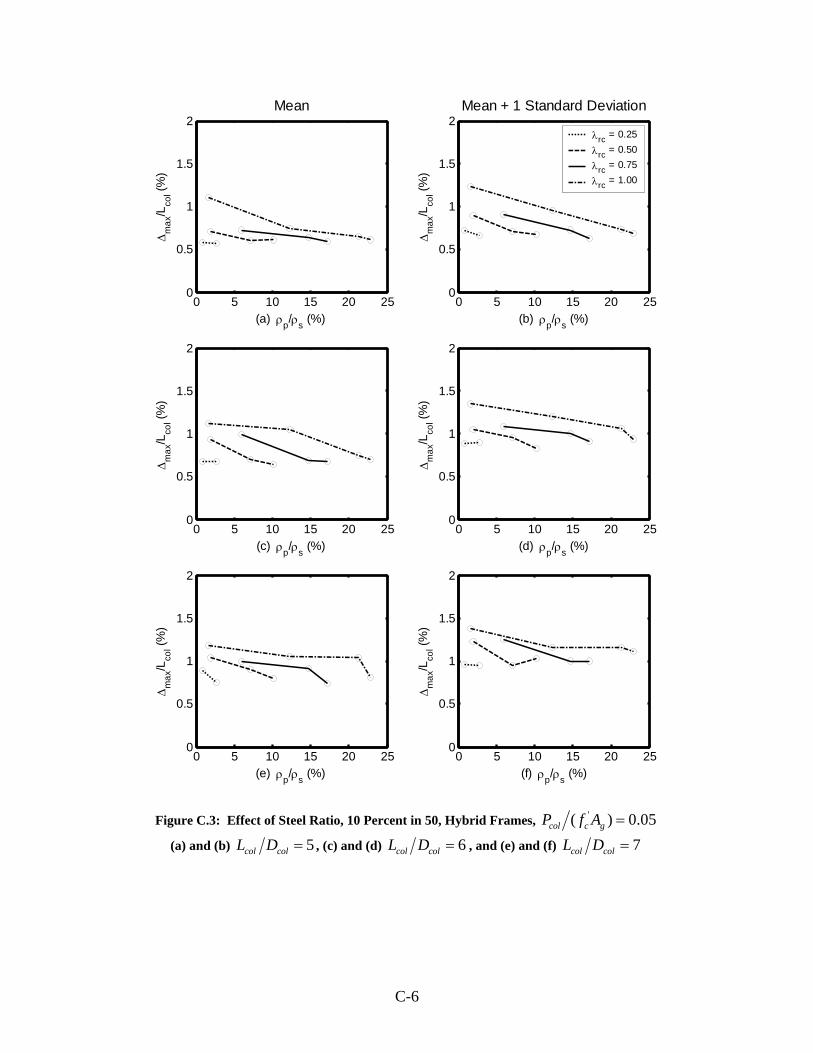
0 5 10 15 20 250
0.5
1
1.5
2
(a) ρp/ρs (%)
Δm
ax/L
col (%
)
Mean
0 5 10 15 20 250
0.5
1
1.5
2
(c) ρp/ρs (%)
Δm
ax/L
col (%
)
0 5 10 15 20 250
0.5
1
1.5
2
(e) ρp/ρs (%)
Δm
ax/L
col (%
)
0 5 10 15 20 250
0.5
1
1.5
2
(b) ρp/ρs (%)
Δm
ax/L
col (%
)
Mean + 1 Standard Deviation
λrc = 0.25λrc = 0.50λrc = 0.75λrc = 1.00
0 5 10 15 20 250
0.5
1
1.5
2
(d) ρp/ρs (%)
Δm
ax/L
col (%
)
0 5 10 15 20 250
0.5
1
1.5
2
(f) ρp/ρs (%)
Δm
ax/L
col (%
)
Figure C.3: Effect of Steel Ratio, 10 Percent in 50, Hybrid Frames, '( ) 0.05col c gP f A =
(a) and (b) 5col colL D = , (c) and (d) 6col colL D = , and (e) and (f) 7col colL D =
C-6
0 5 10 15 20 250
0.5
1
1.5
2
(a) ρp/ρs (%)
Δm
ax/L
col (%
)
Mean
0 5 10 15 20 250
0.5
1
1.5
2
(c) ρp/ρs (%)
Δm
ax/L
col (%
)
0 5 10 15 20 250
0.5
1
1.5
2
(e) ρp/ρs (%)
Δm
ax/L
col (%
)
0 5 10 15 20 250
0.5
1
1.5
2
(b) ρp/ρs (%)
Δm
ax/L
col (%
)
Mean + 1 Standard Deviation
λrc = 0.50λrc = 0.75λrc = 1.00
0 5 10 15 20 250
0.5
1
1.5
2
(d) ρp/ρs (%)
Δm
ax/L
col (%
)
0 5 10 15 20 250
0.5
1
1.5
2
(f) ρp/ρs (%)
Δm
ax/L
col (%
)
Figure C.4: Effect of Steel Ratio, 10 Percent in 50, Hybrid Frames, '( ) 0.10col c gP f A =
(a) and (b) 5col colL D = , (c) and (d) 6col colL D = , and (e) and (f) 7col colL D =
C-7
0 20 40 60 80 100 1200
0.2
0.4
0.6
0.8
1
1.2
1.4
1.6
1.8
2
Fcon004/Ptotal (%)
Mea
n Δ
max
/Lco
l (%)
ρeq = 0.5%ρeq = 1.0%ρeq = 2.0%ρeq = 3.0%
Figure C.5: Effect of Strength on Mean Drift Ratio, 10 Percent
0 20 40 60 80 100 1200
0.2
0.4
0.6
0.8
1
1.2
1.4
1.6
1.8
2
Fcon004/Ptotal (%)
Mea
n +
1 S
td D
evia
tion
Δm
ax/L
col (%
)
λrc = 0.25λrc = 0.50λrc = 0.75λrc = 1.00
Figure C.6: Effect of Strength on Mean Plus One Standard Deviation Drift Ratio, 10 Percent in 50,
Hybrid Frames, '( ) 0.05col c gP f A =
C-8
0 20 40 60 80 100 1200
0.2
0.4
0.6
0.8
1
1.2
1.4
1.6
1.8
2
Fcon004/Ptotal (%)
Mea
n Δ
max
/Lco
l (%)
ρeq = 1.0%ρeq = 2.0%ρeq = 3.0%
Figure C.7: Effect of Strength on Mean Drift Ratio, 10 Percent in 50, Hybrid Frames, '( ) 0.10col c gP f A =
0 20 40 60 80 100 1200
0.2
0.4
0.6
0.8
1
1.2
1.4
1.6
1.8
2
Fcon004/Ptotal (%)
Mea
n +
1 S
td D
evia
tion
Δm
ax/L
col (%
)
λrc = 0.50λrc = 0.75λrc = 1.00
Figure C.8: Effect of Strength on Mean Plus One Standard Deviation Drift Ratio, 10 Percent in 50,
Hybrid Frames, '( ) 0.10col c gP f A =
C-9
0 0.5 1 1.5 2 2.5 30
0.5
1
1.5
2
2.5
3
(Ptotal/Fcon004)1/2
Mea
n Δ
max
/Lco
l (%)
ρeq = 0.5%ρeq = 1.0%ρeq = 2.0%ρeq = 3.0%
Figure C.9: Effect of Stiffness on Mean Drift Ratio, 10 Percent in 50, Hybrid Frames, '( ) 0.05col c gP f A =
0 0.5 1 1.5 2 2.5 30
0.5
1
1.5
2
2.5
3
(Ptotal/Fcon004)1/2
Mea
n +
1 S
td D
evia
tion
Δm
ax/L
col (%
)
λrc = 0.25λrc = 0.50λrc = 0.75λrc = 1.00
Figure C.10: Effect of Stiffness on Mean Plus One Standard Deviation Drift Ratio, 10 Percent in 50,
Hybrid Frames, '( ) 0.05col c gP f A =
C-10
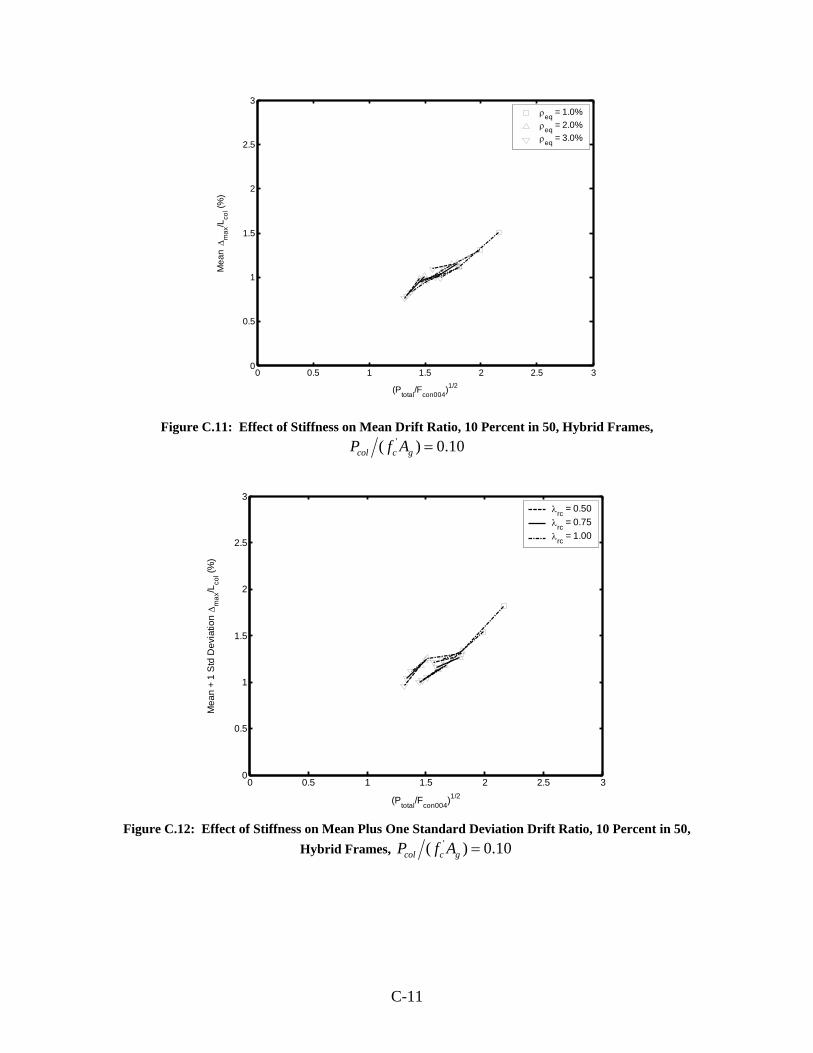
0 0.5 1 1.5 2 2.5 30
0.5
1
1.5
2
2.5
3
(Ptotal/Fcon004)1/2
Mea
n Δ
max
/Lco
l (%)
ρeq = 1.0%ρeq = 2.0%ρeq = 3.0%
Figure C.11: Effect of Stiffness on Mean Drift Ratio, 10 Percent in 50, Hybrid Frames, '( ) 0.10col c gP f A =
0 0.5 1 1.5 2 2.5 30
0.5
1
1.5
2
2.5
3
(Ptotal/Fcon004)1/2
Mea
n +
1 S
td D
evia
tion
Δm
ax/L
col (%
)
λrc = 0.50λrc = 0.75λrc = 1.00
Figure C.12: Effect of Stiffness on Mean Plus One Standard Deviation Drift Ratio, 10 Percent in 50,
Hybrid Frames, '( ) 0.10col c gP f A =
C-11
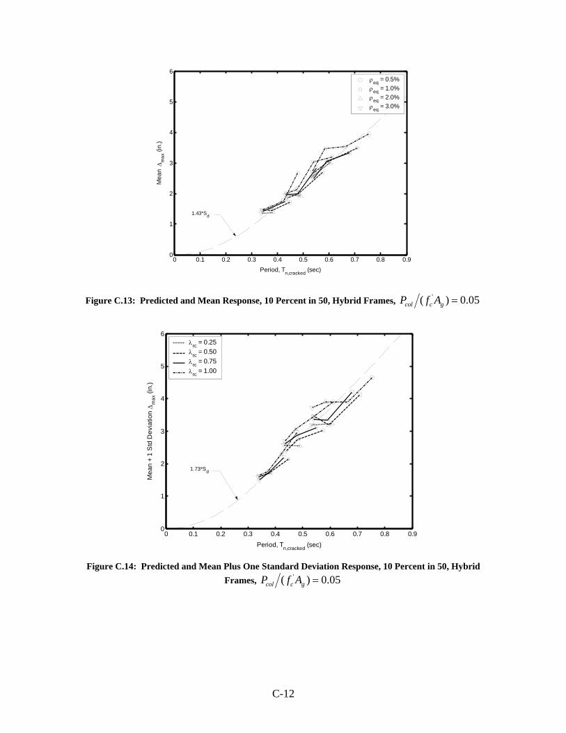
0 0.1 0.2 0.3 0.4 0.5 0.6 0.7 0.8 0.90
1
2
3
4
5
6
Period, Tn,cracked (sec)
Mea
n Δ
max
(in.
)
ρeq = 0.5%ρeq = 1.0%ρeq = 2.0%ρeq = 3.0%
1.43*Sd
Figure C.13: Predicted and Mean Response, 10 Percent in 50, Hybrid Frames, '( ) 0.05col c gP f A =
0 0.1 0.2 0.3 0.4 0.5 0.6 0.7 0.8 0.90
1
2
3
4
5
6
Period, Tn,cracked (sec)
Mea
n +
1 S
td D
evia
tion
Δm
ax (i
n.)
λrc = 0.25λrc = 0.50λrc = 0.75λrc = 1.00
1.73*Sd
Figure C.14: Predicted and Mean Plus One Standard Deviation Response, 10 Percent in 50, Hybrid
Frames, '( ) 0.05col c gP f A =
C-12
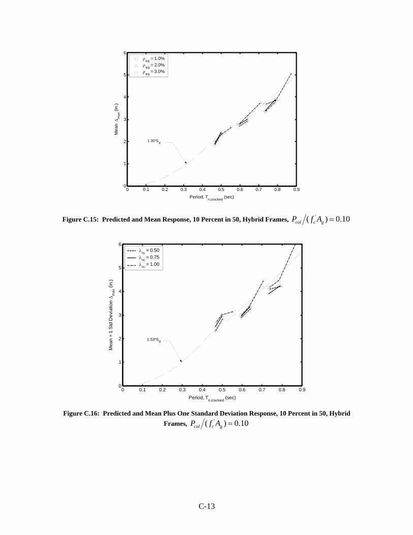
0 0.1 0.2 0.3 0.4 0.5 0.6 0.7 0.8 0.90
1
2
3
4
5
6
Period, Tn,cracked (sec)
Mea
n Δ
max
(in.
)
ρeq = 1.0%ρeq = 2.0%ρeq = 3.0%
1.30*Sd
Figure C.15: Predicted and Mean Response, 10 Percent in 50, Hybrid Frames, '( ) 0.10col c gP f A =
0 0.1 0.2 0.3 0.4 0.5 0.6 0.7 0.8 0.90
1
2
3
4
5
6
Period, Tn,cracked (sec)
Mea
n +
1 S
td D
evia
tion
Δm
ax (i
n.)
λrc = 0.50λrc = 0.75λrc = 1.00
1.53*Sd
Figure C.16: Predicted and Mean Plus One Standard Deviation Response, 10 Percent in 50, Hybrid
Frames, '( ) 0.10col c gP f A =
C-13

C-14
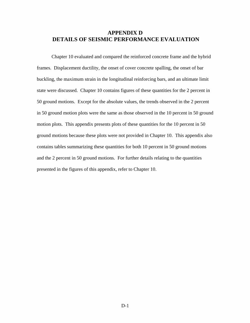
APPENDIX D DETAILS OF SEISMIC PERFORMANCE EVALUATION
Chapter 10 evaluated and compared the reinforced concrete frame and the hybrid
frames. Displacement ductility, the onset of cover concrete spalling, the onset of bar
buckling, the maximum strain in the longitudinal reinforcing bars, and an ultimate limit
state were discussed. Chapter 10 contains figures of these quantities for the 2 percent in
50 ground motions. Except for the absolute values, the trends observed in the 2 percent
in 50 ground motion plots were the same as those observed in the 10 percent in 50 ground
motion plots. This appendix presents plots of these quantities for the 10 percent in 50
ground motions because these plots were not provided in Chapter 10. This appendix also
contains tables summarizing these quantities for both 10 percent in 50 ground motions
and the 2 percent in 50 ground motions. For further details relating to the quantities
presented in the figures of this appendix, refer to Chapter 10.
D-1
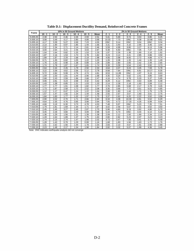
Table D.1: Displacement Ductility Demand, Reinforced Concrete Frames
10 - 1 10 - 2 10 - 3 10 - 4 10 - 5 Mean 2 - 1 2 - 2 2 - 3 2 - 4 2 - 5 Mean5.005.05 2.38 2.50 2.46 2.26 2.93 2.51 5.41 5.69 9.74 3.53 6.86 6.255.005.10 3.08 3.49 4.17 2.80 4.89 3.68 10.33 7.73 DNC 9.38 10.98 9.615.005.15 4.17 3.39 5.27 2.69 7.23 4.55 DNC 9.14 DNC 9.54 DNC 9.345.010.05 2.14 1.90 0.97 1.85 1.44 1.66 3.31 3.40 4.10 2.95 3.46 3.445.010.10 2.32 2.34 2.71 2.14 2.81 2.46 5.59 4.99 9.80 3.27 6.13 5.965.010.15 3.00 2.64 3.21 2.46 3.03 2.87 5.39 5.50 DNC 7.05 7.47 6.355.020.05 1.04 1.64 0.82 1.25 1.53 1.25 1.97 2.26 1.39 1.90 2.10 1.925.020.10 1.87 2.16 1.53 1.74 1.78 1.82 3.23 3.14 4.41 2.85 3.86 3.505.020.15 1.89 1.87 2.29 1.68 2.19 1.98 4.06 3.98 8.05 2.72 4.88 4.745.030.05 0.71 1.35 0.82 1.05 1.22 1.03 1.26 2.08 1.33 1.44 1.35 1.495.030.10 1.76 1.43 0.98 1.38 0.89 1.29 2.89 2.80 2.65 2.42 2.49 2.655.030.15 1.74 1.78 1.87 1.67 1.65 1.74 3.39 3.39 5.54 2.40 3.92 3.736.005.05 2.64 2.44 2.26 1.79 2.50 2.33 4.64 4.07 9.24 3.35 7.59 5.786.005.10 3.22 3.39 4.62 2.56 5.12 3.78 8.68 7.64 DNC 6.81 10.27 8.356.005.15 5.72 2.84 5.99 4.76 4.74 4.81 8.53 11.89 DNC 4.97 9.15 8.636.010.05 1.59 1.53 1.81 1.44 2.06 1.68 3.35 3.24 5.62 2.41 3.85 3.696.010.10 2.68 2.43 2.59 1.96 2.68 2.47 4.16 4.74 9.78 5.20 5.37 5.856.010.15 3.06 2.81 4.23 2.68 4.32 3.42 8.29 6.12 DNC 4.63 6.89 6.486.020.05 1.43 1.38 0.85 1.31 1.03 1.20 2.14 2.28 2.18 1.93 2.08 2.126.020.10 1.77 1.77 1.91 1.58 1.82 1.77 2.76 2.85 5.68 2.17 3.78 3.456.020.15 1.73 1.87 2.58 1.72 2.52 2.08 3.35 3.66 7.72 3.51 6.02 4.856.030.05 1.12 1.17 0.47 1.24 1.22 1.04 2.08 1.83 1.44 1.71 1.75 1.766.030.10 1.57 1.47 1.55 1.34 1.44 1.48 2.55 2.67 3.57 1.93 3.01 2.756.030.15 1.84 1.83 1.77 1.32 1.97 1.75 3.37 2.62 6.20 2.22 3.52 3.587.005.05 2.90 2.02 2.70 1.71 2.66 2.40 6.34 4.38 10.30 4.91 5.52 6.297.005.10 4.64 2.35 4.76 3.95 3.99 3.94 7.05 9.72 17.20 4.26 6.99 9.047.005.15 4.66 3.19 6.30 3.73 4.78 4.53 7.48 9.97 DNC 5.23 7.35 7.517.010.05 1.79 1.81 1.69 1.34 1.71 1.67 3.42 2.56 5.67 2.31 3.52 3.507.010.10 2.45 2.45 3.27 2.45 2.87 2.70 5.96 4.60 9.19 3.92 4.80 5.707.010.15 3.45 2.28 3.80 2.29 3.09 2.98 5.44 5.74 DNC 4.04 6.10 5.337.020.05 1.36 1.29 1.56 1.31 1.39 1.38 2.09 2.12 2.50 1.90 2.34 2.197.020.10 1.49 1.63 1.89 1.37 1.75 1.63 2.80 2.82 5.23 2.07 3.23 3.237.020.15 1.74 2.15 2.74 1.47 1.99 2.02 4.73 3.47 7.05 3.41 3.72 4.487.030.05 1.28 1.43 0.79 1.29 0.99 1.16 1.68 1.83 1.94 1.63 1.72 1.767.030.10 1.31 1.62 1.56 1.44 1.78 1.54 2.83 2.10 4.67 1.91 2.90 2.887.030.15 2.23 1.48 2.17 1.34 1.98 1.84 2.82 3.02 5.07 1.99 4.36 3.45
Note: DNC indicates earthquake analysis did not converge
10% in 50 Ground Motions 2% in 50 Ground MotionsFrame
D-2
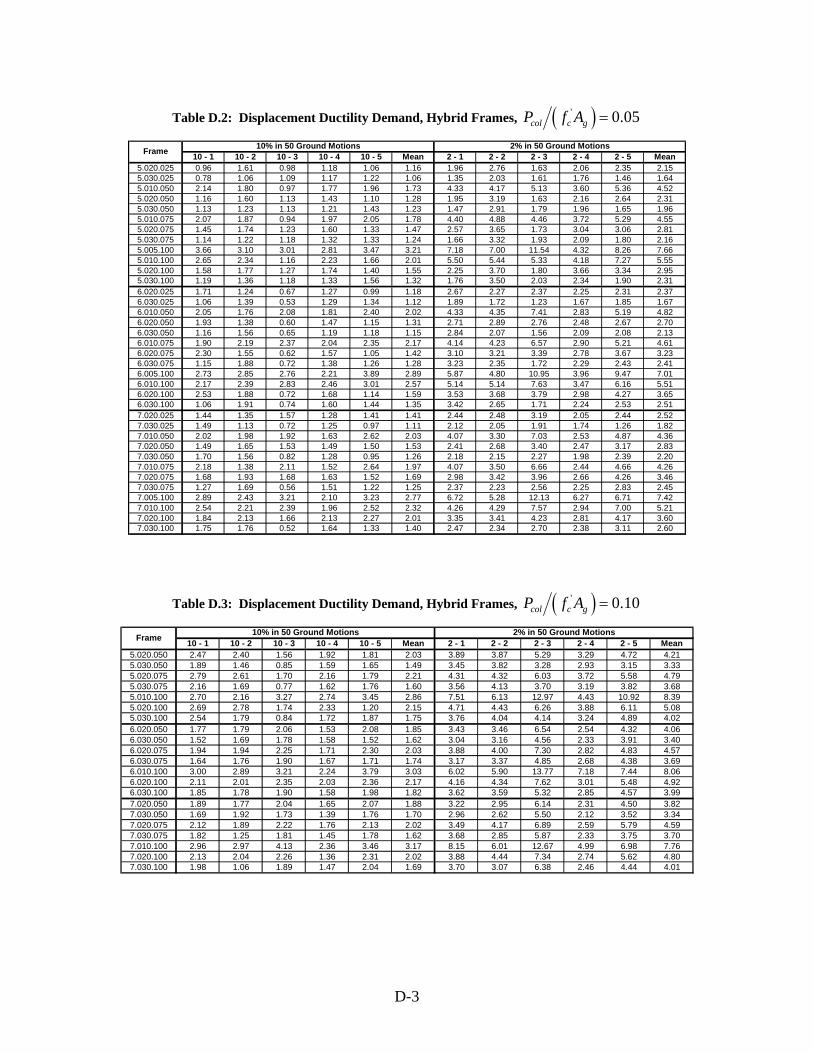
Table D.2: Displacement Ductility Demand, Hybrid Frames, ( )' 0.05col c gP f A =
10 - 1 10 - 2 10 - 3 10 - 4 10 - 5 Mean 2 - 1 2 - 2 2 - 3 2 - 4 2 - 5 Mean5.020.025 0.96 1.61 0.98 1.18 1.06 1.16 1.96 2.76 1.63 2.06 2.35 2.155.030.025 0.78 1.06 1.09 1.17 1.22 1.06 1.35 2.03 1.61 1.76 1.46 1.645.010.050 2.14 1.80 0.97 1.77 1.96 1.73 4.33 4.17 5.13 3.60 5.36 4.525.020.050 1.16 1.60 1.13 1.43 1.10 1.28 1.95 3.19 1.63 2.16 2.64 2.315.030.050 1.13 1.23 1.13 1.21 1.43 1.23 1.47 2.91 1.79 1.96 1.65 1.965.010.075 2.07 1.87 0.94 1.97 2.05 1.78 4.40 4.88 4.46 3.72 5.29 4.555.020.075 1.45 1.74 1.23 1.60 1.33 1.47 2.57 3.65 1.73 3.04 3.06 2.815.030.075 1.14 1.22 1.18 1.32 1.33 1.24 1.66 3.32 1.93 2.09 1.80 2.165.005.100 3.66 3.10 3.01 2.81 3.47 3.21 7.18 7.00 11.54 4.32 8.26 7.665.010.100 2.65 2.34 1.16 2.23 1.66 2.01 5.50 5.44 5.33 4.18 7.27 5.555.020.100 1.58 1.77 1.27 1.74 1.40 1.55 2.25 3.70 1.80 3.66 3.34 2.955.030.100 1.19 1.36 1.18 1.33 1.56 1.32 1.76 3.50 2.03 2.34 1.90 2.316.020.025 1.71 1.24 0.67 1.27 0.99 1.18 2.67 2.27 2.37 2.25 2.31 2.376.030.025 1.06 1.39 0.53 1.29 1.34 1.12 1.89 1.72 1.23 1.67 1.85 1.676.010.050 2.05 1.76 2.08 1.81 2.40 2.02 4.33 4.35 7.41 2.83 5.19 4.826.020.050 1.93 1.38 0.60 1.47 1.15 1.31 2.71 2.89 2.76 2.48 2.67 2.706.030.050 1.16 1.56 0.65 1.19 1.18 1.15 2.84 2.07 1.56 2.09 2.08 2.136.010.075 1.90 2.19 2.37 2.04 2.35 2.17 4.14 4.23 6.57 2.90 5.21 4.616.020.075 2.30 1.55 0.62 1.57 1.05 1.42 3.10 3.21 3.39 2.78 3.67 3.236.030.075 1.15 1.88 0.72 1.38 1.26 1.28 3.23 2.35 1.72 2.29 2.43 2.416.005.100 2.73 2.85 2.76 2.21 3.89 2.89 5.87 4.80 10.95 3.96 9.47 7.016.010.100 2.17 2.39 2.83 2.46 3.01 2.57 5.14 5.14 7.63 3.47 6.16 5.516.020.100 2.53 1.88 0.72 1.68 1.14 1.59 3.53 3.68 3.79 2.98 4.27 3.656.030.100 1.06 1.91 0.74 1.60 1.44 1.35 3.42 2.65 1.71 2.24 2.53 2.517.020.025 1.44 1.35 1.57 1.28 1.41 1.41 2.44 2.48 3.19 2.05 2.44 2.527.030.025 1.49 1.13 0.72 1.25 0.97 1.11 2.12 2.05 1.91 1.74 1.26 1.827.010.050 2.02 1.98 1.92 1.63 2.62 2.03 4.07 3.30 7.03 2.53 4.87 4.367.020.050 1.49 1.65 1.53 1.49 1.50 1.53 2.41 2.68 3.40 2.47 3.17 2.837.030.050 1.70 1.56 0.82 1.28 0.95 1.26 2.18 2.15 2.27 1.98 2.39 2.207.010.075 2.18 1.38 2.11 1.52 2.64 1.97 4.07 3.50 6.66 2.44 4.66 4.267.020.075 1.68 1.93 1.68 1.63 1.52 1.69 2.98 3.42 3.96 2.66 4.26 3.467.030.075 1.27 1.69 0.56 1.51 1.22 1.25 2.37 2.23 2.56 2.25 2.83 2.457.005.100 2.89 2.43 3.21 2.10 3.23 2.77 6.72 5.28 12.13 6.27 6.71 7.427.010.100 2.54 2.21 2.39 1.96 2.52 2.32 4.26 4.29 7.57 2.94 7.00 5.217.020.100 1.84 2.13 1.66 2.13 2.27 2.01 3.35 3.41 4.23 2.81 4.17 3.607.030.100 1.75 1.76 0.52 1.64 1.33 1.40 2.47 2.34 2.70 2.38 3.11 2.60
10% in 50 Ground Motions 2% in 50 Ground MotionsFrame
Table D.3: Displacement Ductility Demand, Hybrid Frames, ( )' 0.10col c gP f A =
10 - 1 10 - 2 10 - 3 10 - 4 10 - 5 Mean 2 - 1 2 - 2 2 - 3 2 - 4 2 - 5 Mean5.020.050 2.47 2.40 1.56 1.92 1.81 2.03 3.89 3.87 5.29 3.29 4.72 4.215.030.050 1.89 1.46 0.85 1.59 1.65 1.49 3.45 3.82 3.28 2.93 3.15 3.335.020.075 2.79 2.61 1.70 2.16 1.79 2.21 4.31 4.32 6.03 3.72 5.58 4.795.030.075 2.16 1.69 0.77 1.62 1.76 1.60 3.56 4.13 3.70 3.19 3.82 3.685.010.100 2.70 2.16 3.27 2.74 3.45 2.86 7.51 6.13 12.97 4.43 10.92 8.395.020.100 2.69 2.78 1.74 2.33 1.20 2.15 4.71 4.43 6.26 3.88 6.11 5.085.030.100 2.54 1.79 0.84 1.72 1.87 1.75 3.76 4.04 4.14 3.24 4.89 4.026.020.050 1.77 1.79 2.06 1.53 2.08 1.85 3.43 3.46 6.54 2.54 4.32 4.066.030.050 1.52 1.69 1.78 1.58 1.52 1.62 3.04 3.16 4.56 2.33 3.91 3.406.020.075 1.94 1.94 2.25 1.71 2.30 2.03 3.88 4.00 7.30 2.82 4.83 4.576.030.075 1.64 1.76 1.90 1.67 1.71 1.74 3.17 3.37 4.85 2.68 4.38 3.696.010.100 3.00 2.89 3.21 2.24 3.79 3.03 6.02 5.90 13.77 7.18 7.44 8.066.020.100 2.11 2.01 2.35 2.03 2.36 2.17 4.16 4.34 7.62 3.01 5.48 4.926.030.100 1.85 1.78 1.90 1.58 1.98 1.82 3.62 3.59 5.32 2.85 4.57 3.997.020.050 1.89 1.77 2.04 1.65 2.07 1.88 3.22 2.95 6.14 2.31 4.50 3.827.030.050 1.69 1.92 1.73 1.39 1.76 1.70 2.96 2.62 5.50 2.12 3.52 3.347.020.075 2.12 1.89 2.22 1.76 2.13 2.02 3.49 4.17 6.89 2.59 5.79 4.597.030.075 1.82 1.25 1.81 1.45 1.78 1.62 3.68 2.85 5.87 2.33 3.75 3.707.010.100 2.96 2.97 4.13 2.36 3.46 3.17 8.15 6.01 12.67 4.99 6.98 7.767.020.100 2.13 2.04 2.26 1.36 2.31 2.02 3.88 4.44 7.34 2.74 5.62 4.807.030.100 1.98 1.06 1.89 1.47 2.04 1.69 3.70 3.07 6.38 2.46 4.44 4.01
10% in 50 Ground Motions 2% in 50 Ground MotionsFrame
D-3
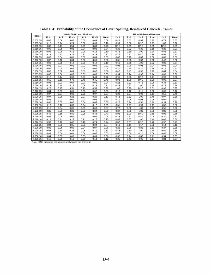
Table D.4: Probability of the Occurrence of Cover Spalling, Reinforced Concrete Frames
10 - 1 10 - 2 10 - 3 10 - 4 10 - 5 Mean 2 - 1 2 - 2 2 - 3 2 - 4 2 - 5 Mean5.005.05 0.05 0.06 0.06 0.05 0.09 0.06 0.46 0.52 0.98 0.15 0.74 0.575.005.10 0.10 0.14 0.24 0.08 0.36 0.18 0.99 0.86 DNC 0.97 1.00 0.965.005.15 0.30 0.17 0.54 0.09 0.88 0.40 DNC 0.99 DNC 0.99 DNC 0.995.010.05 0.06 0.05 0.01 0.04 0.02 0.04 0.20 0.22 0.36 0.15 0.23 0.235.010.10 0.08 0.08 0.12 0.06 0.13 0.10 0.73 0.59 1.00 0.20 0.83 0.675.010.15 0.19 0.13 0.23 0.11 0.19 0.17 0.75 0.77 DNC 0.96 0.98 0.875.020.05 0.02 0.04 0.01 0.02 0.04 0.03 0.07 0.10 0.03 0.06 0.08 0.075.020.10 0.07 0.10 0.04 0.06 0.06 0.06 0.31 0.28 0.63 0.22 0.48 0.385.020.15 0.08 0.08 0.14 0.06 0.12 0.10 0.60 0.58 1.00 0.22 0.81 0.645.030.05 0.01 0.03 0.01 0.02 0.03 0.02 0.03 0.09 0.03 0.04 0.03 0.045.030.10 0.07 0.04 0.02 0.04 0.02 0.04 0.27 0.25 0.21 0.16 0.18 0.215.030.15 0.08 0.08 0.09 0.07 0.07 0.08 0.47 0.47 0.95 0.19 0.64 0.546.005.05 0.07 0.06 0.05 0.03 0.06 0.05 0.34 0.24 0.98 0.14 0.88 0.526.005.10 0.12 0.14 0.33 0.07 0.43 0.22 0.96 0.88 DNC 0.77 0.99 0.906.005.15 0.66 0.11 0.72 0.45 0.45 0.48 0.98 1.00 DNC 0.50 0.99 0.876.010.05 0.03 0.03 0.04 0.03 0.06 0.04 0.23 0.21 0.76 0.09 0.34 0.336.010.10 0.13 0.10 0.12 0.06 0.13 0.11 0.43 0.57 1.00 0.68 0.72 0.686.010.15 0.22 0.17 0.51 0.15 0.53 0.32 1.00 0.90 DNC 0.61 0.96 0.876.020.05 0.04 0.03 0.01 0.03 0.02 0.03 0.10 0.12 0.11 0.08 0.09 0.106.020.10 0.07 0.07 0.08 0.05 0.07 0.07 0.22 0.24 0.92 0.11 0.50 0.406.020.15 0.07 0.09 0.21 0.07 0.20 0.13 0.43 0.52 1.00 0.48 0.97 0.686.030.05 0.02 0.03 0.01 0.03 0.03 0.02 0.11 0.08 0.04 0.06 0.07 0.076.030.10 0.06 0.05 0.06 0.04 0.05 0.05 0.22 0.24 0.51 0.10 0.34 0.286.030.15 0.10 0.10 0.09 0.04 0.12 0.09 0.51 0.27 0.99 0.17 0.56 0.507.005.05 0.10 0.04 0.08 0.03 0.08 0.07 0.72 0.32 1.00 0.43 0.56 0.607.005.10 0.36 0.06 0.38 0.23 0.24 0.25 0.82 0.99 1.00 0.29 0.81 0.787.005.15 0.45 0.16 0.80 0.25 0.48 0.43 0.93 1.00 DNC 0.58 0.92 0.867.010.05 0.05 0.05 0.04 0.02 0.04 0.04 0.28 0.12 0.81 0.09 0.30 0.327.010.10 0.11 0.11 0.25 0.11 0.17 0.15 0.86 0.57 1.00 0.40 0.62 0.697.010.15 0.33 0.10 0.42 0.10 0.24 0.24 0.82 0.87 DNC 0.48 0.92 0.777.020.05 0.04 0.03 0.05 0.03 0.04 0.04 0.10 0.11 0.17 0.08 0.14 0.127.020.10 0.05 0.06 0.09 0.04 0.07 0.06 0.26 0.26 0.89 0.11 0.37 0.387.020.15 0.08 0.14 0.28 0.05 0.11 0.13 0.85 0.50 1.00 0.48 0.59 0.687.030.05 0.03 0.04 0.01 0.04 0.02 0.03 0.07 0.09 0.10 0.06 0.07 0.087.030.10 0.04 0.07 0.06 0.05 0.09 0.06 0.32 0.14 0.86 0.11 0.34 0.357.030.15 0.19 0.06 0.18 0.05 0.14 0.12 0.36 0.43 0.95 0.14 0.84 0.54
Note: DNC indicates earthquake analysis did not converge
10% in 50 Ground Motions 2% in 50 Ground MotionsFrame
D-4
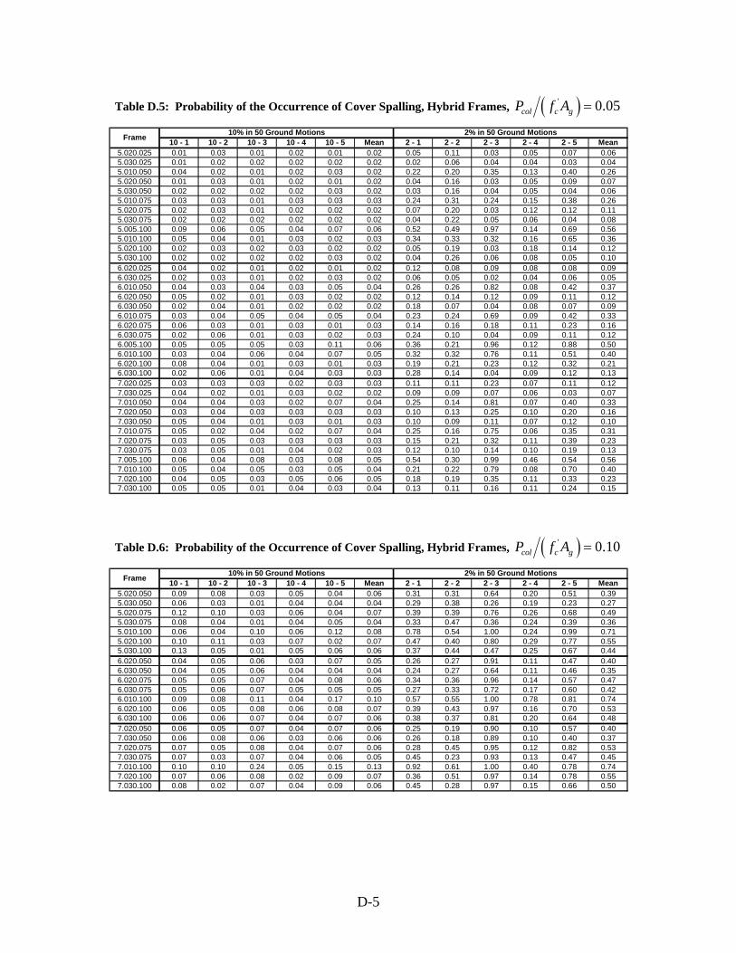
Table D.5: Probability of the Occurrence of Cover Spalling, Hybrid Frames, ( )' 0.05col c gP f A =
10 - 1 10 - 2 10 - 3 10 - 4 10 - 5 Mean 2 - 1 2 - 2 2 - 3 2 - 4 2 - 5 Mean5.020.025 0.01 0.03 0.01 0.02 0.01 0.02 0.05 0.11 0.03 0.05 0.07 0.065.030.025 0.01 0.02 0.02 0.02 0.02 0.02 0.02 0.06 0.04 0.04 0.03 0.045.010.050 0.04 0.02 0.01 0.02 0.03 0.02 0.22 0.20 0.35 0.13 0.40 0.265.020.050 0.01 0.03 0.01 0.02 0.01 0.02 0.04 0.16 0.03 0.05 0.09 0.075.030.050 0.02 0.02 0.02 0.02 0.03 0.02 0.03 0.16 0.04 0.05 0.04 0.065.010.075 0.03 0.03 0.01 0.03 0.03 0.03 0.24 0.31 0.24 0.15 0.38 0.265.020.075 0.02 0.03 0.01 0.02 0.02 0.02 0.07 0.20 0.03 0.12 0.12 0.115.030.075 0.02 0.02 0.02 0.02 0.02 0.02 0.04 0.22 0.05 0.06 0.04 0.085.005.100 0.09 0.06 0.05 0.04 0.07 0.06 0.52 0.49 0.97 0.14 0.69 0.565.010.100 0.05 0.04 0.01 0.03 0.02 0.03 0.34 0.33 0.32 0.16 0.65 0.365.020.100 0.02 0.03 0.02 0.03 0.02 0.02 0.05 0.19 0.03 0.18 0.14 0.125.030.100 0.02 0.02 0.02 0.02 0.03 0.02 0.04 0.26 0.06 0.08 0.05 0.106.020.025 0.04 0.02 0.01 0.02 0.01 0.02 0.12 0.08 0.09 0.08 0.08 0.096.030.025 0.02 0.03 0.01 0.02 0.03 0.02 0.06 0.05 0.02 0.04 0.06 0.056.010.050 0.04 0.03 0.04 0.03 0.05 0.04 0.26 0.26 0.82 0.08 0.42 0.376.020.050 0.05 0.02 0.01 0.03 0.02 0.02 0.12 0.14 0.12 0.09 0.11 0.126.030.050 0.02 0.04 0.01 0.02 0.02 0.02 0.18 0.07 0.04 0.08 0.07 0.096.010.075 0.03 0.04 0.05 0.04 0.05 0.04 0.23 0.24 0.69 0.09 0.42 0.336.020.075 0.06 0.03 0.01 0.03 0.01 0.03 0.14 0.16 0.18 0.11 0.23 0.166.030.075 0.02 0.06 0.01 0.03 0.02 0.03 0.24 0.10 0.04 0.09 0.11 0.126.005.100 0.05 0.05 0.05 0.03 0.11 0.06 0.36 0.21 0.96 0.12 0.88 0.506.010.100 0.03 0.04 0.06 0.04 0.07 0.05 0.32 0.32 0.76 0.11 0.51 0.406.020.100 0.08 0.04 0.01 0.03 0.01 0.03 0.19 0.21 0.23 0.12 0.32 0.216.030.100 0.02 0.06 0.01 0.04 0.03 0.03 0.28 0.14 0.04 0.09 0.12 0.137.020.025 0.03 0.03 0.03 0.02 0.03 0.03 0.11 0.11 0.23 0.07 0.11 0.127.030.025 0.04 0.02 0.01 0.03 0.02 0.02 0.09 0.09 0.07 0.06 0.03 0.077.010.050 0.04 0.04 0.03 0.02 0.07 0.04 0.25 0.14 0.81 0.07 0.40 0.337.020.050 0.03 0.04 0.03 0.03 0.03 0.03 0.10 0.13 0.25 0.10 0.20 0.167.030.050 0.05 0.04 0.01 0.03 0.01 0.03 0.10 0.09 0.11 0.07 0.12 0.107.010.075 0.05 0.02 0.04 0.02 0.07 0.04 0.25 0.16 0.75 0.06 0.35 0.317.020.075 0.03 0.05 0.03 0.03 0.03 0.03 0.15 0.21 0.32 0.11 0.39 0.237.030.075 0.03 0.05 0.01 0.04 0.02 0.03 0.12 0.10 0.14 0.10 0.19 0.137.005.100 0.06 0.04 0.08 0.03 0.08 0.05 0.54 0.30 0.99 0.46 0.54 0.567.010.100 0.05 0.04 0.05 0.03 0.05 0.04 0.21 0.22 0.79 0.08 0.70 0.407.020.100 0.04 0.05 0.03 0.05 0.06 0.05 0.18 0.19 0.35 0.11 0.33 0.237.030.100 0.05 0.05 0.01 0.04 0.03 0.04 0.13 0.11 0.16 0.11 0.24 0.15
10% in 50 Ground Motions 2% in 50 Ground MotionsFrame
Table D.6: Probability of the Occurrence of Cover Spalling, Hybrid Frames, ( )' 0.10col c gP f A =
10 - 1 10 - 2 10 - 3 10 - 4 10 - 5 Mean 2 - 1 2 - 2 2 - 3 2 - 4 2 - 5 Mean5.020.050 0.09 0.08 0.03 0.05 0.04 0.06 0.31 0.31 0.64 0.20 0.51 0.395.030.050 0.06 0.03 0.01 0.04 0.04 0.04 0.29 0.38 0.26 0.19 0.23 0.275.020.075 0.12 0.10 0.03 0.06 0.04 0.07 0.39 0.39 0.76 0.26 0.68 0.495.030.075 0.08 0.04 0.01 0.04 0.05 0.04 0.33 0.47 0.36 0.24 0.39 0.365.010.100 0.06 0.04 0.10 0.06 0.12 0.08 0.78 0.54 1.00 0.24 0.99 0.715.020.100 0.10 0.11 0.03 0.07 0.02 0.07 0.47 0.40 0.80 0.29 0.77 0.555.030.100 0.13 0.05 0.01 0.05 0.06 0.06 0.37 0.44 0.47 0.25 0.67 0.446.020.050 0.04 0.05 0.06 0.03 0.07 0.05 0.26 0.27 0.91 0.11 0.47 0.406.030.050 0.04 0.05 0.06 0.04 0.04 0.04 0.24 0.27 0.64 0.11 0.46 0.356.020.075 0.05 0.05 0.07 0.04 0.08 0.06 0.34 0.36 0.96 0.14 0.57 0.476.030.075 0.05 0.06 0.07 0.05 0.05 0.05 0.27 0.33 0.72 0.17 0.60 0.426.010.100 0.09 0.08 0.11 0.04 0.17 0.10 0.57 0.55 1.00 0.78 0.81 0.746.020.100 0.06 0.05 0.08 0.06 0.08 0.07 0.39 0.43 0.97 0.16 0.70 0.536.030.100 0.06 0.06 0.07 0.04 0.07 0.06 0.38 0.37 0.81 0.20 0.64 0.487.020.050 0.06 0.05 0.07 0.04 0.07 0.06 0.25 0.19 0.90 0.10 0.57 0.407.030.050 0.06 0.08 0.06 0.03 0.06 0.06 0.26 0.18 0.89 0.10 0.40 0.377.020.075 0.07 0.05 0.08 0.04 0.07 0.06 0.28 0.45 0.95 0.12 0.82 0.537.030.075 0.07 0.03 0.07 0.04 0.06 0.05 0.45 0.23 0.93 0.13 0.47 0.457.010.100 0.10 0.10 0.24 0.05 0.15 0.13 0.92 0.61 1.00 0.40 0.78 0.747.020.100 0.07 0.06 0.08 0.02 0.09 0.07 0.36 0.51 0.97 0.14 0.78 0.557.030.100 0.08 0.02 0.07 0.04 0.09 0.06 0.45 0.28 0.97 0.15 0.66 0.50
10% in 50 Ground Motions 2% in 50 Ground MotionsFrame
D-5
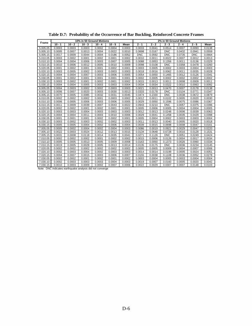
Table D.7: Probability of the Occurrence of Bar Buckling, Reinforced Concrete Frames
10 - 1 10 - 2 10 - 3 10 - 4 10 - 5 Mean 2 - 1 2 - 2 2 - 3 2 - 4 2 - 5 Mean5.005.05 0.0003 0.0003 0.0003 0.0002 0.0004 0.0003 0.0033 0.0041 0.0514 0.0007 0.0093 0.01385.005.10 0.0005 0.0007 0.0013 0.0004 0.0022 0.0010 0.0698 0.0167 DNC 0.0432 0.0941 0.05595.005.15 0.0017 0.0009 0.0044 0.0004 0.0186 0.0052 DNC 0.0592 DNC 0.0735 DNC 0.06645.010.05 0.0003 0.0002 0.0001 0.0002 0.0001 0.0002 0.0010 0.0011 0.0022 0.0007 0.0012 0.00135.010.10 0.0004 0.0004 0.0006 0.0003 0.0007 0.0005 0.0088 0.0053 0.1356 0.0011 0.0136 0.03295.010.15 0.0010 0.0006 0.0012 0.0005 0.0010 0.0009 0.0098 0.0108 DNC 0.0358 0.0478 0.02605.020.05 0.0001 0.0002 0.0001 0.0001 0.0002 0.0001 0.0003 0.0005 0.0002 0.0003 0.0004 0.00035.020.10 0.0003 0.0005 0.0002 0.0003 0.0003 0.0003 0.0018 0.0016 0.0062 0.0011 0.0035 0.00285.020.15 0.0004 0.0004 0.0007 0.0003 0.0006 0.0005 0.0054 0.0050 0.1465 0.0012 0.0126 0.03415.030.05 0.0001 0.0002 0.0001 0.0001 0.0001 0.0001 0.0002 0.0005 0.0002 0.0002 0.0002 0.00025.030.10 0.0003 0.0002 0.0001 0.0002 0.0001 0.0002 0.0015 0.0013 0.0011 0.0008 0.0009 0.00115.030.15 0.0004 0.0004 0.0005 0.0003 0.0003 0.0004 0.0034 0.0034 0.0322 0.0010 0.0063 0.00926.005.05 0.0004 0.0003 0.0002 0.0002 0.0003 0.0003 0.0021 0.0013 0.0470 0.0007 0.0178 0.01386.005.10 0.0006 0.0007 0.0020 0.0003 0.0030 0.0013 0.0333 0.0178 DNC 0.0104 0.0771 0.03476.005.15 0.0070 0.0005 0.0085 0.0032 0.0031 0.0045 0.0474 0.2330 DNC 0.0038 0.0672 0.08796.010.05 0.0002 0.0002 0.0002 0.0001 0.0003 0.0002 0.0012 0.0011 0.0102 0.0005 0.0020 0.00306.010.10 0.0006 0.0005 0.0006 0.0003 0.0006 0.0005 0.0029 0.0050 0.1596 0.0075 0.0086 0.03676.010.15 0.0011 0.0009 0.0039 0.0007 0.0043 0.0022 0.0943 0.0210 DNC 0.0057 0.0375 0.03966.020.05 0.0002 0.0002 0.0001 0.0002 0.0001 0.0001 0.0005 0.0006 0.0005 0.0004 0.0004 0.00056.020.10 0.0003 0.0003 0.0004 0.0003 0.0003 0.0003 0.0012 0.0013 0.0248 0.0006 0.0039 0.00636.020.15 0.0004 0.0004 0.0011 0.0003 0.0010 0.0006 0.0029 0.0041 0.1458 0.0035 0.0429 0.03986.030.05 0.0001 0.0001 0.0001 0.0002 0.0002 0.0001 0.0005 0.0004 0.0002 0.0003 0.0003 0.00046.030.10 0.0003 0.0002 0.0003 0.0002 0.0002 0.0003 0.0011 0.0013 0.0040 0.0005 0.0020 0.00186.030.15 0.0005 0.0005 0.0004 0.0002 0.0006 0.0004 0.0039 0.0015 0.0698 0.0008 0.0047 0.01617.005.05 0.0005 0.0002 0.0004 0.0002 0.0004 0.0003 0.0086 0.0019 0.0921 0.0029 0.0047 0.02207.005.10 0.0022 0.0003 0.0024 0.0012 0.0013 0.0015 0.0134 0.0648 0.6728 0.0016 0.0128 0.15317.005.15 0.0031 0.0008 0.0118 0.0014 0.0035 0.0041 0.0271 0.1126 DNC 0.0051 0.0249 0.04247.010.05 0.0002 0.0002 0.0002 0.0001 0.0002 0.0002 0.0015 0.0006 0.0126 0.0004 0.0017 0.00347.010.10 0.0005 0.0005 0.0013 0.0005 0.0009 0.0008 0.0163 0.0050 0.1373 0.0026 0.0060 0.03347.010.15 0.0019 0.0005 0.0028 0.0005 0.0013 0.0014 0.0135 0.0175 DNC 0.0036 0.0234 0.01457.020.05 0.0002 0.0002 0.0002 0.0002 0.0002 0.0002 0.0005 0.0005 0.0009 0.0004 0.0007 0.00067.020.10 0.0002 0.0003 0.0004 0.0002 0.0003 0.0003 0.0014 0.0014 0.0199 0.0005 0.0024 0.00517.020.15 0.0004 0.0007 0.0015 0.0003 0.0006 0.0007 0.0155 0.0038 0.1108 0.0036 0.0052 0.02787.030.05 0.0002 0.0002 0.0001 0.0002 0.0001 0.0002 0.0003 0.0004 0.0005 0.0003 0.0004 0.00047.030.10 0.0002 0.0003 0.0003 0.0003 0.0004 0.0003 0.0019 0.0007 0.0160 0.0005 0.0020 0.00427.030.15 0.0010 0.0003 0.0009 0.0002 0.0007 0.0006 0.0022 0.0029 0.0307 0.0007 0.0148 0.0103
Note: DNC indicates earthquake analysis did not converge
10% in 50 Ground Motions 2% in 50 Ground MotionsFrame
D-6
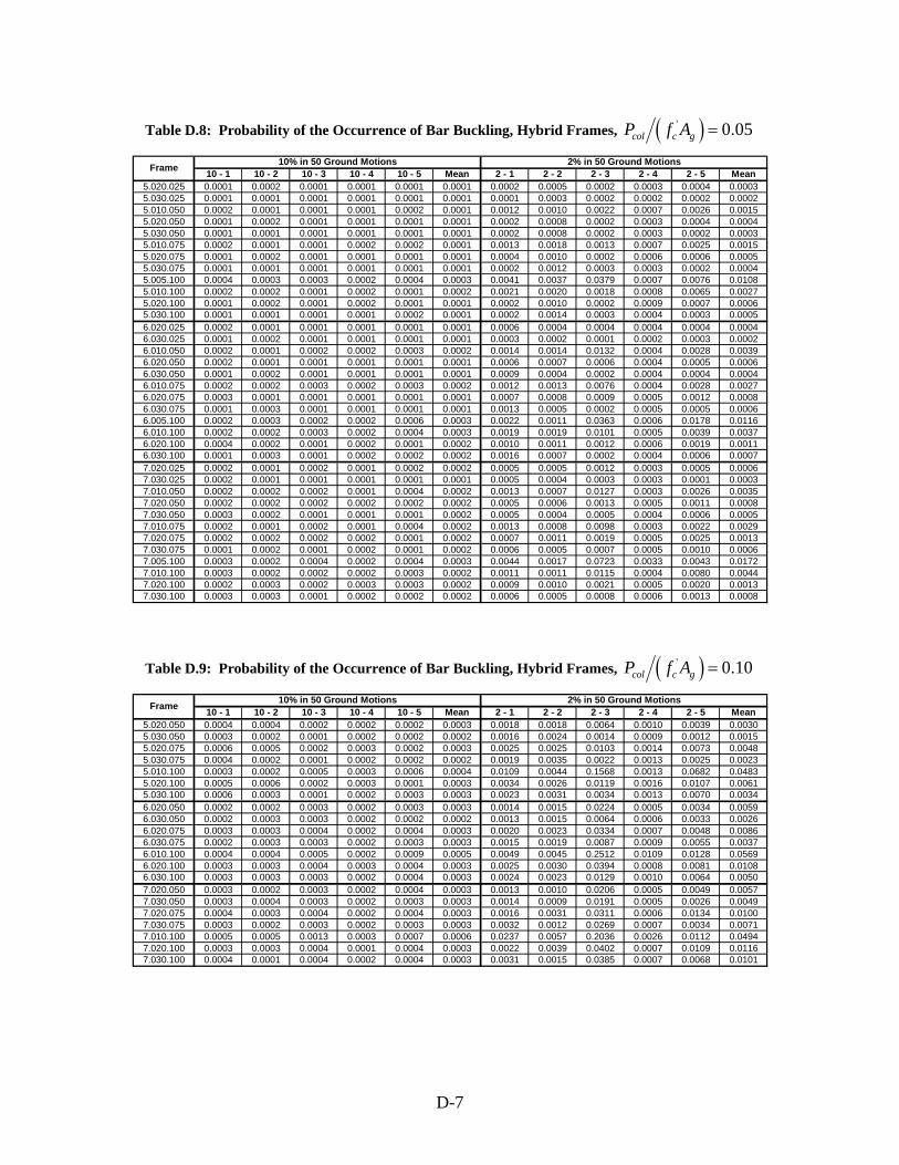
Table D.8: Probability of the Occurrence of Bar Buckling, Hybrid Frames, ( )' 0.05col c gP f A =
10 - 1 10 - 2 10 - 3 10 - 4 10 - 5 Mean 2 - 1 2 - 2 2 - 3 2 - 4 2 - 5 Mean5.020.025 0.0001 0.0002 0.0001 0.0001 0.0001 0.0001 0.0002 0.0005 0.0002 0.0003 0.0004 0.00035.030.025 0.0001 0.0001 0.0001 0.0001 0.0001 0.0001 0.0001 0.0003 0.0002 0.0002 0.0002 0.00025.010.050 0.0002 0.0001 0.0001 0.0001 0.0002 0.0001 0.0012 0.0010 0.0022 0.0007 0.0026 0.00155.020.050 0.0001 0.0002 0.0001 0.0001 0.0001 0.0001 0.0002 0.0008 0.0002 0.0003 0.0004 0.00045.030.050 0.0001 0.0001 0.0001 0.0001 0.0001 0.0001 0.0002 0.0008 0.0002 0.0003 0.0002 0.00035.010.075 0.0002 0.0001 0.0001 0.0002 0.0002 0.0001 0.0013 0.0018 0.0013 0.0007 0.0025 0.00155.020.075 0.0001 0.0002 0.0001 0.0001 0.0001 0.0001 0.0004 0.0010 0.0002 0.0006 0.0006 0.00055.030.075 0.0001 0.0001 0.0001 0.0001 0.0001 0.0001 0.0002 0.0012 0.0003 0.0003 0.0002 0.00045.005.100 0.0004 0.0003 0.0003 0.0002 0.0004 0.0003 0.0041 0.0037 0.0379 0.0007 0.0076 0.01085.010.100 0.0002 0.0002 0.0001 0.0002 0.0001 0.0002 0.0021 0.0020 0.0018 0.0008 0.0065 0.00275.020.100 0.0001 0.0002 0.0001 0.0002 0.0001 0.0001 0.0002 0.0010 0.0002 0.0009 0.0007 0.00065.030.100 0.0001 0.0001 0.0001 0.0001 0.0002 0.0001 0.0002 0.0014 0.0003 0.0004 0.0003 0.00056.020.025 0.0002 0.0001 0.0001 0.0001 0.0001 0.0001 0.0006 0.0004 0.0004 0.0004 0.0004 0.00046.030.025 0.0001 0.0002 0.0001 0.0001 0.0001 0.0001 0.0003 0.0002 0.0001 0.0002 0.0003 0.00026.010.050 0.0002 0.0001 0.0002 0.0002 0.0003 0.0002 0.0014 0.0014 0.0132 0.0004 0.0028 0.00396.020.050 0.0002 0.0001 0.0001 0.0001 0.0001 0.0001 0.0006 0.0007 0.0006 0.0004 0.0005 0.00066.030.050 0.0001 0.0002 0.0001 0.0001 0.0001 0.0001 0.0009 0.0004 0.0002 0.0004 0.0004 0.00046.010.075 0.0002 0.0002 0.0003 0.0002 0.0003 0.0002 0.0012 0.0013 0.0076 0.0004 0.0028 0.00276.020.075 0.0003 0.0001 0.0001 0.0001 0.0001 0.0001 0.0007 0.0008 0.0009 0.0005 0.0012 0.00086.030.075 0.0001 0.0003 0.0001 0.0001 0.0001 0.0001 0.0013 0.0005 0.0002 0.0005 0.0005 0.00066.005.100 0.0002 0.0003 0.0002 0.0002 0.0006 0.0003 0.0022 0.0011 0.0363 0.0006 0.0178 0.01166.010.100 0.0002 0.0002 0.0003 0.0002 0.0004 0.0003 0.0019 0.0019 0.0101 0.0005 0.0039 0.00376.020.100 0.0004 0.0002 0.0001 0.0002 0.0001 0.0002 0.0010 0.0011 0.0012 0.0006 0.0019 0.00116.030.100 0.0001 0.0003 0.0001 0.0002 0.0002 0.0002 0.0016 0.0007 0.0002 0.0004 0.0006 0.00077.020.025 0.0002 0.0001 0.0002 0.0001 0.0002 0.0002 0.0005 0.0005 0.0012 0.0003 0.0005 0.00067.030.025 0.0002 0.0001 0.0001 0.0001 0.0001 0.0001 0.0005 0.0004 0.0003 0.0003 0.0001 0.00037.010.050 0.0002 0.0002 0.0002 0.0001 0.0004 0.0002 0.0013 0.0007 0.0127 0.0003 0.0026 0.00357.020.050 0.0002 0.0002 0.0002 0.0002 0.0002 0.0002 0.0005 0.0006 0.0013 0.0005 0.0011 0.00087.030.050 0.0003 0.0002 0.0001 0.0001 0.0001 0.0002 0.0005 0.0004 0.0005 0.0004 0.0006 0.00057.010.075 0.0002 0.0001 0.0002 0.0001 0.0004 0.0002 0.0013 0.0008 0.0098 0.0003 0.0022 0.00297.020.075 0.0002 0.0002 0.0002 0.0002 0.0001 0.0002 0.0007 0.0011 0.0019 0.0005 0.0025 0.00137.030.075 0.0001 0.0002 0.0001 0.0002 0.0001 0.0002 0.0006 0.0005 0.0007 0.0005 0.0010 0.00067.005.100 0.0003 0.0002 0.0004 0.0002 0.0004 0.0003 0.0044 0.0017 0.0723 0.0033 0.0043 0.01727.010.100 0.0003 0.0002 0.0002 0.0002 0.0003 0.0002 0.0011 0.0011 0.0115 0.0004 0.0080 0.00447.020.100 0.0002 0.0003 0.0002 0.0003 0.0003 0.0002 0.0009 0.0010 0.0021 0.0005 0.0020 0.00137.030.100 0.0003 0.0003 0.0001 0.0002 0.0002 0.0002 0.0006 0.0005 0.0008 0.0006 0.0013 0.0008
10% in 50 Ground Motions 2% in 50 Ground MotionsFrame
Table D.9: Probability of the Occurrence of Bar Buckling, Hybrid Frames, ( )' 0.10col c gP f A =
10 - 1 10 - 2 10 - 3 10 - 4 10 - 5 Mean 2 - 1 2 - 2 2 - 3 2 - 4 2 - 5 Mean5.020.050 0.0004 0.0004 0.0002 0.0002 0.0002 0.0003 0.0018 0.0018 0.0064 0.0010 0.0039 0.00305.030.050 0.0003 0.0002 0.0001 0.0002 0.0002 0.0002 0.0016 0.0024 0.0014 0.0009 0.0012 0.00155.020.075 0.0006 0.0005 0.0002 0.0003 0.0002 0.0003 0.0025 0.0025 0.0103 0.0014 0.0073 0.00485.030.075 0.0004 0.0002 0.0001 0.0002 0.0002 0.0002 0.0019 0.0035 0.0022 0.0013 0.0025 0.00235.010.100 0.0003 0.0002 0.0005 0.0003 0.0006 0.0004 0.0109 0.0044 0.1568 0.0013 0.0682 0.04835.020.100 0.0005 0.0006 0.0002 0.0003 0.0001 0.0003 0.0034 0.0026 0.0119 0.0016 0.0107 0.00615.030.100 0.0006 0.0003 0.0001 0.0002 0.0003 0.0003 0.0023 0.0031 0.0034 0.0013 0.0070 0.00346.020.050 0.0002 0.0002 0.0003 0.0002 0.0003 0.0003 0.0014 0.0015 0.0224 0.0005 0.0034 0.00596.030.050 0.0002 0.0003 0.0003 0.0002 0.0002 0.0002 0.0013 0.0015 0.0064 0.0006 0.0033 0.00266.020.075 0.0003 0.0003 0.0004 0.0002 0.0004 0.0003 0.0020 0.0023 0.0334 0.0007 0.0048 0.00866.030.075 0.0002 0.0003 0.0003 0.0002 0.0003 0.0003 0.0015 0.0019 0.0087 0.0009 0.0055 0.00376.010.100 0.0004 0.0004 0.0005 0.0002 0.0009 0.0005 0.0049 0.0045 0.2512 0.0109 0.0128 0.05696.020.100 0.0003 0.0003 0.0004 0.0003 0.0004 0.0003 0.0025 0.0030 0.0394 0.0008 0.0081 0.01086.030.100 0.0003 0.0003 0.0003 0.0002 0.0004 0.0003 0.0024 0.0023 0.0129 0.0010 0.0064 0.00507.020.050 0.0003 0.0002 0.0003 0.0002 0.0004 0.0003 0.0013 0.0010 0.0206 0.0005 0.0049 0.00577.030.050 0.0003 0.0004 0.0003 0.0002 0.0003 0.0003 0.0014 0.0009 0.0191 0.0005 0.0026 0.00497.020.075 0.0004 0.0003 0.0004 0.0002 0.0004 0.0003 0.0016 0.0031 0.0311 0.0006 0.0134 0.01007.030.075 0.0003 0.0002 0.0003 0.0002 0.0003 0.0003 0.0032 0.0012 0.0269 0.0007 0.0034 0.00717.010.100 0.0005 0.0005 0.0013 0.0003 0.0007 0.0006 0.0237 0.0057 0.2036 0.0026 0.0112 0.04947.020.100 0.0003 0.0003 0.0004 0.0001 0.0004 0.0003 0.0022 0.0039 0.0402 0.0007 0.0109 0.01167.030.100 0.0004 0.0001 0.0004 0.0002 0.0004 0.0003 0.0031 0.0015 0.0385 0.0007 0.0068 0.0101
10% in 50 Ground Motions 2% in 50 Ground MotionsFrame
D-7
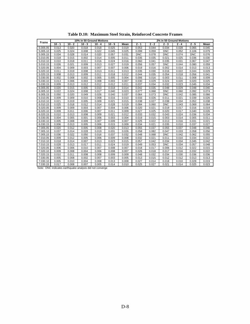
Table D.10: Maximum Steel Strain, Reinforced Concrete Frames
10 - 1 10 - 2 10 - 3 10 - 4 10 - 5 Mean 2 - 1 2 - 2 2 - 3 2 - 4 2 - 5 Mean5.005.05 0.013 0.020 0.018 0.018 0.025 0.019 0.053 0.044 0.034 0.028 0.065 0.0455.005.10 0.025 0.024 0.008 0.022 0.045 0.025 0.099 0.059 DNC 0.052 0.106 0.0795.005.15 0.034 0.028 0.014 0.020 0.057 0.031 DNC 0.078 DNC 0.074 DNC 0.0765.010.05 0.018 0.015 0.002 0.014 0.005 0.011 0.035 0.035 0.021 0.025 0.036 0.0305.010.10 0.010 0.018 0.011 0.016 0.024 0.016 0.060 0.041 0.035 0.031 0.067 0.0475.010.15 0.026 0.021 0.009 0.013 0.027 0.019 0.056 0.057 DNC 0.044 0.080 0.0595.020.05 0.004 0.009 0.003 0.007 0.007 0.006 0.019 0.016 0.002 0.014 0.013 0.0135.020.10 0.011 0.019 0.008 0.013 0.011 0.013 0.035 0.030 0.016 0.022 0.044 0.0295.020.15 0.008 0.013 0.009 0.011 0.018 0.012 0.044 0.035 0.054 0.018 0.056 0.0415.030.05 0.002 0.008 0.002 0.005 0.005 0.004 0.006 0.016 0.003 0.011 0.008 0.0095.030.10 0.013 0.006 0.003 0.008 0.003 0.007 0.030 0.029 0.024 0.020 0.020 0.0255.030.15 0.009 0.013 0.012 0.012 0.012 0.011 0.037 0.034 0.032 0.023 0.045 0.0346.005.05 0.020 0.015 0.005 0.010 0.018 0.014 0.042 0.035 0.048 0.029 0.048 0.0406.005.10 0.022 0.024 0.008 0.017 0.040 0.023 0.077 0.068 DNC 0.060 0.092 0.0746.005.15 0.050 0.020 0.049 0.026 0.040 0.037 0.064 0.073 DNC 0.042 0.085 0.0666.010.05 0.009 0.009 0.010 0.008 0.016 0.010 0.033 0.026 0.011 0.021 0.039 0.0266.010.10 0.021 0.019 0.005 0.009 0.021 0.015 0.038 0.027 0.038 0.034 0.052 0.0386.010.15 0.025 0.018 0.012 0.014 0.028 0.019 0.084 0.060 DNC 0.043 0.069 0.0646.020.05 0.009 0.009 0.003 0.007 0.004 0.006 0.020 0.021 0.019 0.017 0.016 0.0196.020.10 0.009 0.011 0.006 0.007 0.011 0.009 0.027 0.025 0.020 0.017 0.040 0.0266.020.15 0.010 0.013 0.008 0.009 0.021 0.012 0.033 0.032 0.043 0.024 0.036 0.0346.030.05 0.004 0.005 0.001 0.006 0.003 0.004 0.019 0.015 0.003 0.014 0.005 0.0116.030.10 0.005 0.008 0.009 0.007 0.009 0.007 0.025 0.022 0.013 0.016 0.031 0.0216.030.15 0.006 0.013 0.005 0.006 0.015 0.009 0.034 0.021 0.035 0.010 0.037 0.0277.005.05 0.020 0.012 0.005 0.008 0.020 0.013 0.055 0.037 0.055 0.037 0.048 0.0467.005.10 0.037 0.014 0.028 0.019 0.031 0.026 0.058 0.082 0.047 0.033 0.058 0.0567.005.15 0.036 0.022 0.050 0.016 0.037 0.032 0.048 0.068 DNC 0.042 0.062 0.0557.010.05 0.009 0.012 0.005 0.006 0.009 0.008 0.032 0.021 0.011 0.010 0.034 0.0227.010.10 0.018 0.014 0.007 0.013 0.023 0.015 0.057 0.042 0.034 0.034 0.045 0.0427.010.15 0.028 0.013 0.017 0.011 0.024 0.019 0.049 0.053 DNC 0.034 0.057 0.0487.020.05 0.006 0.006 0.010 0.007 0.008 0.007 0.018 0.017 0.006 0.012 0.022 0.0157.020.10 0.009 0.008 0.004 0.006 0.008 0.007 0.026 0.018 0.017 0.016 0.032 0.0227.020.15 0.010 0.011 0.008 0.008 0.009 0.009 0.048 0.032 0.034 0.030 0.036 0.0367.030.05 0.005 0.008 0.002 0.007 0.003 0.005 0.013 0.015 0.012 0.012 0.013 0.0137.030.10 0.005 0.010 0.004 0.008 0.013 0.008 0.027 0.014 0.018 0.010 0.028 0.0197.030.15 0.017 0.008 0.007 0.005 0.014 0.010 0.025 0.027 0.021 0.014 0.025 0.023
Note: DNC indicates earthquake analysis did not converge
10% in 50 Ground Motions 2% in 50 Ground MotionsFrame
D-8
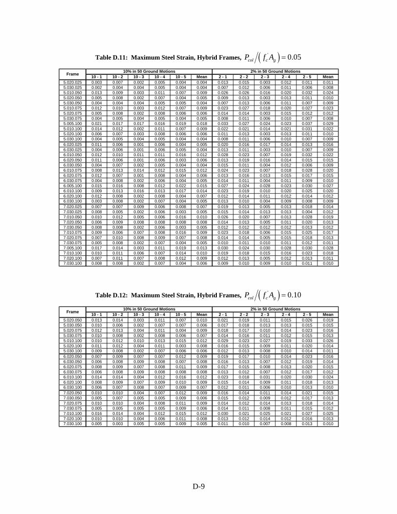
Table D.11: Maximum Steel Strain, Hybrid Frames, ( )' 0.05col c gP f A =
10 - 1 10 - 2 10 - 3 10 - 4 10 - 5 Mean 2 - 1 2 - 2 2 - 3 2 - 4 2 - 5 Mean5.020.025 0.003 0.007 0.002 0.005 0.004 0.004 0.013 0.015 0.003 0.012 0.011 0.0115.030.025 0.002 0.004 0.004 0.005 0.004 0.004 0.007 0.012 0.006 0.011 0.006 0.0085.010.050 0.013 0.009 0.003 0.011 0.007 0.009 0.026 0.026 0.016 0.020 0.032 0.0245.020.050 0.005 0.008 0.002 0.007 0.004 0.005 0.009 0.013 0.003 0.013 0.011 0.0105.030.050 0.004 0.004 0.004 0.005 0.005 0.004 0.007 0.013 0.006 0.011 0.007 0.0095.010.075 0.012 0.010 0.003 0.012 0.007 0.009 0.023 0.027 0.018 0.020 0.027 0.0235.020.075 0.005 0.008 0.002 0.008 0.006 0.006 0.014 0.014 0.003 0.015 0.012 0.0125.030.075 0.004 0.005 0.004 0.005 0.004 0.005 0.008 0.011 0.006 0.010 0.007 0.0085.005.100 0.021 0.017 0.017 0.016 0.019 0.018 0.033 0.027 0.024 0.023 0.037 0.0295.010.100 0.014 0.012 0.002 0.011 0.007 0.009 0.022 0.021 0.014 0.021 0.031 0.0225.020.100 0.006 0.007 0.003 0.008 0.006 0.006 0.011 0.013 0.003 0.013 0.011 0.0105.030.100 0.004 0.005 0.004 0.005 0.004 0.004 0.008 0.011 0.006 0.010 0.007 0.0096.020.025 0.011 0.006 0.001 0.006 0.004 0.005 0.020 0.016 0.017 0.014 0.013 0.0166.030.025 0.004 0.006 0.001 0.006 0.005 0.004 0.013 0.011 0.003 0.010 0.007 0.0096.010.050 0.012 0.010 0.011 0.011 0.016 0.012 0.028 0.023 0.007 0.019 0.032 0.0226.020.050 0.011 0.006 0.001 0.006 0.003 0.006 0.013 0.019 0.016 0.014 0.015 0.0156.030.050 0.004 0.007 0.002 0.005 0.004 0.004 0.015 0.011 0.004 0.012 0.006 0.0096.010.075 0.008 0.013 0.014 0.012 0.015 0.012 0.024 0.023 0.007 0.018 0.028 0.0206.020.075 0.012 0.007 0.001 0.008 0.004 0.006 0.013 0.016 0.013 0.015 0.017 0.0156.030.075 0.004 0.008 0.002 0.006 0.004 0.005 0.014 0.011 0.004 0.011 0.009 0.0106.005.100 0.015 0.016 0.008 0.012 0.022 0.015 0.027 0.024 0.028 0.023 0.030 0.0276.010.100 0.009 0.013 0.016 0.013 0.017 0.014 0.023 0.019 0.010 0.020 0.025 0.0206.020.100 0.012 0.008 0.002 0.008 0.004 0.007 0.012 0.014 0.011 0.012 0.014 0.0126.030.100 0.003 0.008 0.002 0.007 0.004 0.005 0.013 0.010 0.004 0.009 0.008 0.0097.020.025 0.007 0.007 0.009 0.006 0.008 0.007 0.019 0.013 0.005 0.013 0.018 0.0147.030.025 0.008 0.005 0.002 0.006 0.003 0.005 0.015 0.014 0.013 0.013 0.004 0.0127.010.050 0.010 0.012 0.005 0.006 0.016 0.010 0.026 0.020 0.007 0.013 0.028 0.0197.020.050 0.006 0.009 0.008 0.008 0.008 0.008 0.014 0.013 0.005 0.011 0.020 0.0137.030.050 0.008 0.008 0.002 0.006 0.003 0.005 0.012 0.012 0.012 0.012 0.013 0.0127.010.075 0.009 0.006 0.007 0.008 0.016 0.009 0.023 0.018 0.006 0.015 0.025 0.0177.020.075 0.007 0.010 0.008 0.009 0.007 0.008 0.014 0.014 0.005 0.015 0.018 0.0137.030.075 0.005 0.008 0.002 0.007 0.004 0.005 0.010 0.011 0.010 0.011 0.012 0.0117.005.100 0.017 0.014 0.003 0.011 0.019 0.013 0.030 0.024 0.030 0.028 0.030 0.0287.010.100 0.010 0.011 0.006 0.007 0.014 0.010 0.019 0.018 0.015 0.016 0.023 0.0187.020.100 0.007 0.011 0.007 0.008 0.012 0.009 0.012 0.013 0.005 0.012 0.013 0.0117.030.100 0.008 0.008 0.002 0.007 0.004 0.006 0.009 0.010 0.009 0.010 0.011 0.010
10% in 50 Ground Motions 2% in 50 Ground MotionsFrame
Table D.12: Maximum Steel Strain, Hybrid Frames, ( )' 0.10col c gP f A =
10 - 1 10 - 2 10 - 3 10 - 4 10 - 5 Mean 2 - 1 2 - 2 2 - 3 2 - 4 2 - 5 Mean5.020.050 0.013 0.014 0.003 0.011 0.007 0.010 0.021 0.019 0.011 0.015 0.026 0.0195.030.050 0.010 0.006 0.002 0.007 0.007 0.006 0.017 0.018 0.013 0.013 0.015 0.0155.020.075 0.012 0.013 0.004 0.011 0.004 0.009 0.018 0.017 0.010 0.014 0.023 0.0165.030.075 0.010 0.008 0.002 0.008 0.006 0.007 0.014 0.016 0.011 0.012 0.015 0.0135.010.100 0.010 0.012 0.010 0.013 0.015 0.012 0.029 0.023 0.027 0.019 0.033 0.0265.020.100 0.011 0.012 0.004 0.011 0.003 0.008 0.016 0.015 0.009 0.011 0.020 0.0145.030.100 0.009 0.008 0.002 0.007 0.006 0.006 0.012 0.013 0.008 0.010 0.014 0.0116.020.050 0.007 0.009 0.007 0.007 0.012 0.009 0.019 0.017 0.010 0.014 0.023 0.0166.030.050 0.006 0.008 0.009 0.008 0.007 0.008 0.016 0.013 0.007 0.012 0.019 0.0146.020.075 0.008 0.009 0.007 0.008 0.011 0.009 0.017 0.015 0.008 0.013 0.020 0.0156.030.075 0.006 0.008 0.009 0.008 0.008 0.008 0.013 0.012 0.007 0.012 0.017 0.0126.010.100 0.014 0.014 0.004 0.012 0.016 0.012 0.023 0.018 0.031 0.020 0.030 0.0246.020.100 0.008 0.009 0.007 0.009 0.010 0.009 0.015 0.014 0.009 0.011 0.018 0.0136.030.100 0.006 0.007 0.008 0.007 0.009 0.007 0.012 0.011 0.006 0.010 0.013 0.0107.020.050 0.010 0.010 0.004 0.007 0.012 0.009 0.016 0.014 0.011 0.014 0.021 0.0157.030.050 0.005 0.007 0.005 0.005 0.009 0.006 0.015 0.012 0.009 0.012 0.017 0.0137.020.075 0.010 0.010 0.004 0.008 0.011 0.009 0.014 0.012 0.014 0.013 0.018 0.0147.030.075 0.005 0.005 0.005 0.005 0.009 0.006 0.014 0.011 0.008 0.011 0.015 0.0127.010.100 0.016 0.014 0.004 0.012 0.015 0.012 0.030 0.021 0.025 0.021 0.027 0.0257.020.100 0.010 0.010 0.004 0.006 0.011 0.008 0.013 0.012 0.014 0.012 0.016 0.0137.030.100 0.005 0.003 0.005 0.005 0.009 0.005 0.011 0.010 0.007 0.008 0.013 0.010
10% in 50 Ground Motions 2% in 50 Ground MotionsFrame
D-9
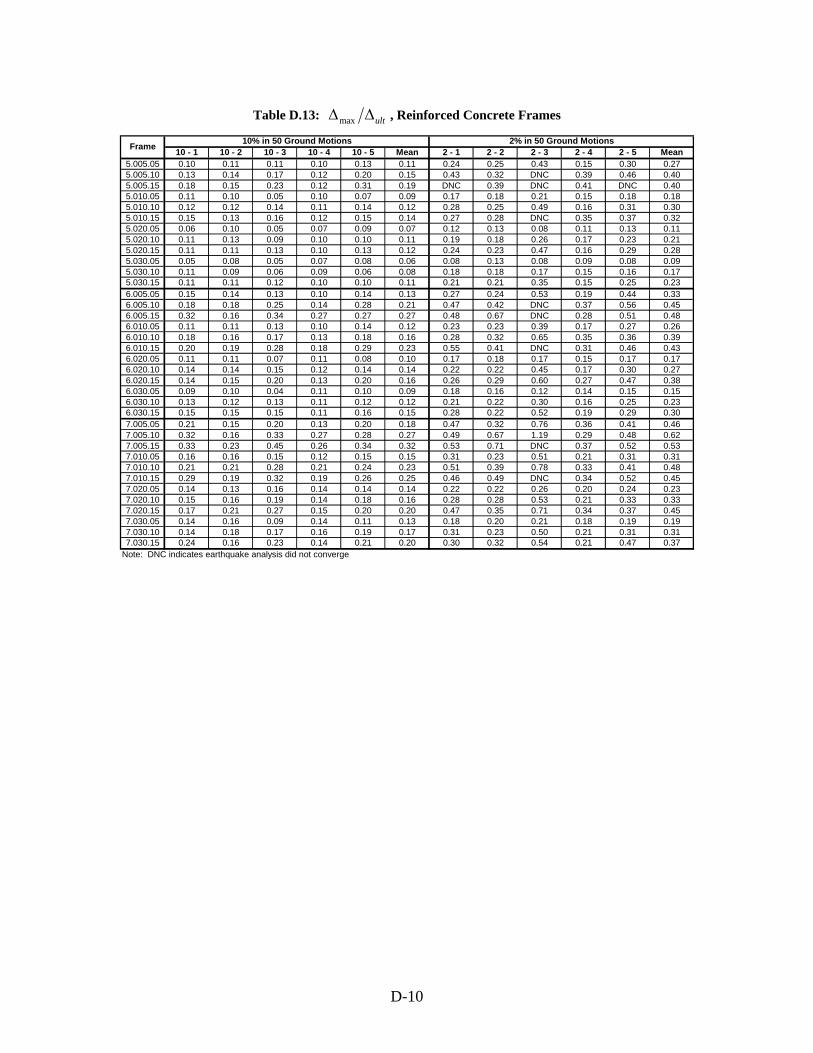
Table D.13: max ultΔ Δ , Reinforced Concrete Frames
10 - 1 10 - 2 10 - 3 10 - 4 10 - 5 Mean 2 - 1 2 - 2 2 - 3 2 - 4 2 - 5 Mean5.005.05 0.10 0.11 0.11 0.10 0.13 0.11 0.24 0.25 0.43 0.15 0.30 0.275.005.10 0.13 0.14 0.17 0.12 0.20 0.15 0.43 0.32 DNC 0.39 0.46 0.405.005.15 0.18 0.15 0.23 0.12 0.31 0.19 DNC 0.39 DNC 0.41 DNC 0.405.010.05 0.11 0.10 0.05 0.10 0.07 0.09 0.17 0.18 0.21 0.15 0.18 0.185.010.10 0.12 0.12 0.14 0.11 0.14 0.12 0.28 0.25 0.49 0.16 0.31 0.305.010.15 0.15 0.13 0.16 0.12 0.15 0.14 0.27 0.28 DNC 0.35 0.37 0.325.020.05 0.06 0.10 0.05 0.07 0.09 0.07 0.12 0.13 0.08 0.11 0.13 0.115.020.10 0.11 0.13 0.09 0.10 0.10 0.11 0.19 0.18 0.26 0.17 0.23 0.215.020.15 0.11 0.11 0.13 0.10 0.13 0.12 0.24 0.23 0.47 0.16 0.29 0.285.030.05 0.05 0.08 0.05 0.07 0.08 0.06 0.08 0.13 0.08 0.09 0.08 0.095.030.10 0.11 0.09 0.06 0.09 0.06 0.08 0.18 0.18 0.17 0.15 0.16 0.175.030.15 0.11 0.11 0.12 0.10 0.10 0.11 0.21 0.21 0.35 0.15 0.25 0.236.005.05 0.15 0.14 0.13 0.10 0.14 0.13 0.27 0.24 0.53 0.19 0.44 0.336.005.10 0.18 0.18 0.25 0.14 0.28 0.21 0.47 0.42 DNC 0.37 0.56 0.456.005.15 0.32 0.16 0.34 0.27 0.27 0.27 0.48 0.67 DNC 0.28 0.51 0.486.010.05 0.11 0.11 0.13 0.10 0.14 0.12 0.23 0.23 0.39 0.17 0.27 0.266.010.10 0.18 0.16 0.17 0.13 0.18 0.16 0.28 0.32 0.65 0.35 0.36 0.396.010.15 0.20 0.19 0.28 0.18 0.29 0.23 0.55 0.41 DNC 0.31 0.46 0.436.020.05 0.11 0.11 0.07 0.11 0.08 0.10 0.17 0.18 0.17 0.15 0.17 0.176.020.10 0.14 0.14 0.15 0.12 0.14 0.14 0.22 0.22 0.45 0.17 0.30 0.276.020.15 0.14 0.15 0.20 0.13 0.20 0.16 0.26 0.29 0.60 0.27 0.47 0.386.030.05 0.09 0.10 0.04 0.11 0.10 0.09 0.18 0.16 0.12 0.14 0.15 0.156.030.10 0.13 0.12 0.13 0.11 0.12 0.12 0.21 0.22 0.30 0.16 0.25 0.236.030.15 0.15 0.15 0.15 0.11 0.16 0.15 0.28 0.22 0.52 0.19 0.29 0.307.005.05 0.21 0.15 0.20 0.13 0.20 0.18 0.47 0.32 0.76 0.36 0.41 0.467.005.10 0.32 0.16 0.33 0.27 0.28 0.27 0.49 0.67 1.19 0.29 0.48 0.627.005.15 0.33 0.23 0.45 0.26 0.34 0.32 0.53 0.71 DNC 0.37 0.52 0.537.010.05 0.16 0.16 0.15 0.12 0.15 0.15 0.31 0.23 0.51 0.21 0.31 0.317.010.10 0.21 0.21 0.28 0.21 0.24 0.23 0.51 0.39 0.78 0.33 0.41 0.487.010.15 0.29 0.19 0.32 0.19 0.26 0.25 0.46 0.49 DNC 0.34 0.52 0.457.020.05 0.14 0.13 0.16 0.14 0.14 0.14 0.22 0.22 0.26 0.20 0.24 0.237.020.10 0.15 0.16 0.19 0.14 0.18 0.16 0.28 0.28 0.53 0.21 0.33 0.337.020.15 0.17 0.21 0.27 0.15 0.20 0.20 0.47 0.35 0.71 0.34 0.37 0.457.030.05 0.14 0.16 0.09 0.14 0.11 0.13 0.18 0.20 0.21 0.18 0.19 0.197.030.10 0.14 0.18 0.17 0.16 0.19 0.17 0.31 0.23 0.50 0.21 0.31 0.317.030.15 0.24 0.16 0.23 0.14 0.21 0.20 0.30 0.32 0.54 0.21 0.47 0.37
Note: DNC indicates earthquake analysis did not converge
10% in 50 Ground Motions 2% in 50 Ground MotionsFrame
D-10
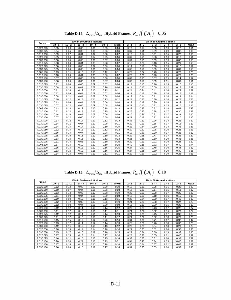
Table D.14: max ultΔ Δ , Hybrid Frames, ( )' 0.05col c gP f A =
10 - 1 10 - 2 10 - 3 10 - 4 10 - 5 Mean 2 - 1 2 - 2 2 - 3 2 - 4 2 - 5 Mean5.020.025 0.05 0.08 0.05 0.06 0.05 0.06 0.10 0.14 0.08 0.10 0.12 0.115.030.025 0.04 0.06 0.06 0.06 0.06 0.06 0.07 0.11 0.09 0.09 0.08 0.095.010.050 0.09 0.07 0.04 0.07 0.08 0.07 0.18 0.17 0.21 0.15 0.22 0.195.020.050 0.05 0.08 0.05 0.07 0.05 0.06 0.09 0.15 0.08 0.10 0.12 0.115.030.050 0.06 0.06 0.06 0.06 0.07 0.06 0.07 0.15 0.09 0.10 0.08 0.105.010.075 0.08 0.08 0.04 0.08 0.08 0.07 0.18 0.20 0.18 0.15 0.21 0.185.020.075 0.06 0.08 0.05 0.07 0.06 0.06 0.11 0.16 0.08 0.13 0.13 0.125.030.075 0.05 0.06 0.06 0.06 0.06 0.06 0.08 0.16 0.09 0.10 0.09 0.105.005.100 0.13 0.11 0.10 0.10 0.12 0.11 0.25 0.24 0.40 0.15 0.29 0.265.010.100 0.10 0.09 0.04 0.08 0.06 0.07 0.20 0.20 0.20 0.15 0.27 0.205.020.100 0.07 0.07 0.05 0.07 0.06 0.06 0.09 0.15 0.07 0.15 0.14 0.125.030.100 0.06 0.06 0.05 0.06 0.07 0.06 0.08 0.16 0.09 0.11 0.09 0.116.020.025 0.12 0.08 0.05 0.09 0.07 0.08 0.18 0.15 0.16 0.15 0.16 0.166.030.025 0.08 0.10 0.04 0.09 0.10 0.08 0.14 0.13 0.09 0.12 0.13 0.126.010.050 0.11 0.10 0.12 0.10 0.13 0.11 0.24 0.24 0.41 0.16 0.29 0.276.020.050 0.12 0.09 0.04 0.09 0.07 0.08 0.17 0.18 0.18 0.16 0.17 0.176.030.050 0.08 0.11 0.04 0.08 0.08 0.08 0.19 0.14 0.11 0.14 0.14 0.146.010.075 0.10 0.12 0.13 0.11 0.13 0.12 0.23 0.23 0.36 0.16 0.28 0.256.020.075 0.13 0.09 0.04 0.09 0.06 0.08 0.18 0.19 0.20 0.16 0.22 0.196.030.075 0.07 0.12 0.05 0.09 0.08 0.08 0.21 0.15 0.11 0.15 0.16 0.156.005.100 0.13 0.13 0.13 0.10 0.18 0.13 0.27 0.22 0.51 0.18 0.44 0.326.010.100 0.11 0.12 0.14 0.12 0.15 0.13 0.25 0.25 0.38 0.17 0.30 0.276.020.100 0.14 0.10 0.04 0.09 0.06 0.09 0.20 0.21 0.21 0.17 0.24 0.206.030.100 0.07 0.12 0.05 0.10 0.09 0.08 0.21 0.17 0.11 0.14 0.16 0.167.020.025 0.13 0.12 0.14 0.11 0.12 0.13 0.22 0.22 0.28 0.18 0.22 0.227.030.025 0.14 0.11 0.07 0.12 0.09 0.11 0.20 0.19 0.18 0.17 0.12 0.177.010.050 0.14 0.14 0.14 0.12 0.19 0.15 0.29 0.24 0.50 0.18 0.35 0.317.020.050 0.12 0.14 0.13 0.12 0.12 0.13 0.20 0.22 0.28 0.20 0.26 0.237.030.050 0.15 0.14 0.07 0.11 0.08 0.11 0.19 0.19 0.20 0.17 0.21 0.197.010.075 0.15 0.10 0.15 0.11 0.19 0.14 0.29 0.25 0.47 0.17 0.33 0.307.020.075 0.13 0.15 0.13 0.12 0.12 0.13 0.23 0.26 0.30 0.20 0.32 0.267.030.075 0.11 0.14 0.05 0.13 0.10 0.10 0.20 0.19 0.21 0.19 0.24 0.207.005.100 0.17 0.14 0.19 0.12 0.19 0.16 0.40 0.31 0.72 0.37 0.40 0.447.010.100 0.16 0.14 0.15 0.12 0.16 0.15 0.27 0.27 0.48 0.19 0.44 0.337.020.100 0.13 0.15 0.12 0.15 0.16 0.14 0.24 0.25 0.30 0.20 0.30 0.267.030.100 0.14 0.14 0.04 0.13 0.11 0.11 0.20 0.19 0.22 0.19 0.25 0.21
10% in 50 Ground Motions 2% in 50 Ground MotionsFrame
Table D.15: max ultΔ Δ , Hybrid Frames, ( )' 0.10col c gP f A =
10 - 1 10 - 2 10 - 3 10 - 4 10 - 5 Mean 2 - 1 2 - 2 2 - 3 2 - 4 2 - 5 Mean5.020.050 0.12 0.12 0.08 0.09 0.09 0.10 0.19 0.19 0.26 0.16 0.23 0.205.030.050 0.10 0.07 0.04 0.08 0.08 0.08 0.18 0.20 0.17 0.15 0.16 0.175.020.075 0.13 0.12 0.08 0.10 0.08 0.10 0.20 0.20 0.28 0.17 0.26 0.225.030.075 0.11 0.08 0.04 0.08 0.09 0.08 0.18 0.20 0.18 0.16 0.19 0.185.010.100 0.10 0.08 0.13 0.11 0.13 0.11 0.29 0.24 0.50 0.17 0.42 0.325.020.100 0.12 0.12 0.08 0.10 0.05 0.10 0.21 0.20 0.28 0.17 0.27 0.235.030.100 0.12 0.08 0.04 0.08 0.09 0.08 0.18 0.19 0.20 0.15 0.23 0.196.020.050 0.12 0.12 0.14 0.10 0.14 0.12 0.23 0.23 0.43 0.17 0.28 0.276.030.050 0.11 0.12 0.12 0.11 0.11 0.11 0.21 0.22 0.32 0.16 0.27 0.246.020.075 0.12 0.12 0.14 0.11 0.14 0.13 0.24 0.25 0.45 0.17 0.30 0.286.030.075 0.11 0.12 0.13 0.11 0.11 0.12 0.21 0.22 0.32 0.18 0.29 0.256.010.100 0.15 0.15 0.17 0.12 0.20 0.16 0.31 0.30 0.71 0.37 0.38 0.426.020.100 0.13 0.12 0.14 0.12 0.14 0.13 0.25 0.26 0.46 0.18 0.33 0.296.030.100 0.12 0.11 0.12 0.10 0.13 0.12 0.23 0.23 0.34 0.18 0.29 0.257.020.050 0.16 0.15 0.17 0.14 0.18 0.16 0.27 0.25 0.52 0.20 0.38 0.337.030.050 0.15 0.17 0.16 0.12 0.16 0.15 0.27 0.24 0.50 0.19 0.32 0.307.020.075 0.17 0.15 0.18 0.14 0.17 0.16 0.28 0.33 0.55 0.21 0.46 0.377.030.075 0.16 0.11 0.16 0.13 0.15 0.14 0.32 0.25 0.51 0.20 0.32 0.327.010.100 0.20 0.20 0.27 0.16 0.23 0.21 0.54 0.40 0.84 0.33 0.46 0.517.020.100 0.17 0.16 0.17 0.10 0.18 0.16 0.30 0.34 0.57 0.21 0.43 0.377.030.100 0.16 0.09 0.16 0.12 0.17 0.14 0.31 0.25 0.53 0.20 0.37 0.33
10% in 50 Ground Motions 2% in 50 Ground MotionsFrame
D-11
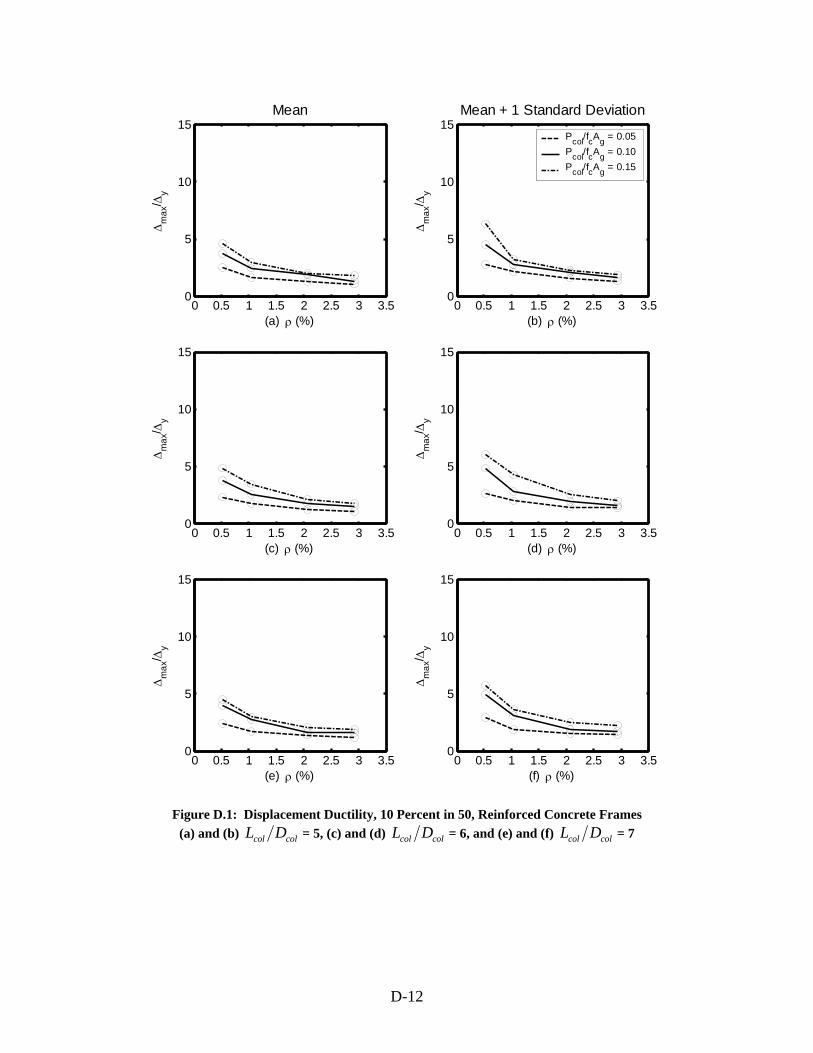
0 0.5 1 1.5 2 2.5 3 3.50
5
10
15
(a) ρ (%)
Δm
ax/ Δ
y
Mean
0 0.5 1 1.5 2 2.5 3 3.50
5
10
15
(c) ρ (%)
Δm
ax/ Δ
y
0 0.5 1 1.5 2 2.5 3 3.50
5
10
15
(e) ρ (%)
Δm
ax/ Δ
y
0 0.5 1 1.5 2 2.5 3 3.50
5
10
15
(b) ρ (%)
Δm
ax/ Δ
y
Mean + 1 Standard Deviation
Pcol/fcAg = 0.05Pcol/fcAg = 0.10Pcol/fcAg = 0.15
0 0.5 1 1.5 2 2.5 3 3.50
5
10
15
(d) ρ (%)
Δm
ax/ Δ
y
0 0.5 1 1.5 2 2.5 3 3.50
5
10
15
(f) ρ (%)
Δm
ax/ Δ
y
Figure D.1: Displacement Ductility, 10 Percent in 50, Reinforced Concrete Frames (a) and (b) col colL D = 5, (c) and (d) col colL D = 6, and (e) and (f) col colL D = 7
D-12

0 0.5 1 1.5 2 2.5 3 3.50
5
10
15
(a) ρeq (%)
Δm
ax/ Δ
y
Mean
0 0.5 1 1.5 2 2.5 3 3.50
5
10
15
(c) ρeq (%)
Δm
ax/ Δ
y
0 0.5 1 1.5 2 2.5 3 3.50
5
10
15
(e) ρeq (%)
Δm
ax/ Δ
y
0 0.5 1 1.5 2 2.5 3 3.50
5
10
15
(b) ρeq (%)
Δm
ax/ Δ
y
Mean + 1 Standard Deviation
λrc = 0.25λrc = 0.50λrc = 0.75λrc = 1.00
0 0.5 1 1.5 2 2.5 3 3.50
5
10
15
(d) ρeq (%)
Δm
ax/ Δ
y
0 0.5 1 1.5 2 2.5 3 3.50
5
10
15
(f) ρeq (%)
Δm
ax/ Δ
y
Figure D.2: Displacement Ductility, 10 Percent in 50, Hybrid Frames, ( )' 0.05col c gP f A =
(a) and (b) col colL D = 5, (c) and (d) col colL D = 6, and (e) and (f) col colL D = 7
D-13
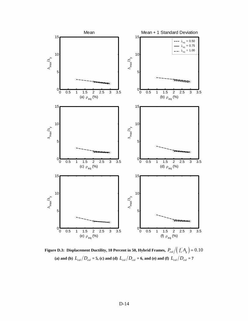
0 0.5 1 1.5 2 2.5 3 3.50
5
10
15
(a) ρeq (%)
Δm
ax/ Δ
y
Mean
0 0.5 1 1.5 2 2.5 3 3.50
5
10
15
(c) ρeq (%)
Δm
ax/ Δ
y
0 0.5 1 1.5 2 2.5 3 3.50
5
10
15
(e) ρeq (%)
Δm
ax/ Δ
y
0 0.5 1 1.5 2 2.5 3 3.50
5
10
15
(b) ρeq (%)
Δm
ax/ Δ
y
Mean + 1 Standard Deviation
λrc = 0.50λrc = 0.75λrc = 1.00
0 0.5 1 1.5 2 2.5 3 3.50
5
10
15
(d) ρeq (%)
Δm
ax/ Δ
y
0 0.5 1 1.5 2 2.5 3 3.50
5
10
15
(f) ρeq (%)
Δm
ax/ Δ
y
Figure D.3: Displacement Ductility, 10 Percent in 50, Hybrid Frames, ( )' 0.10col c gP f A =
(a) and (b) col colL D = 5, (c) and (d) col colL D = 6, and (e) and (f) col colL D = 7
D-14
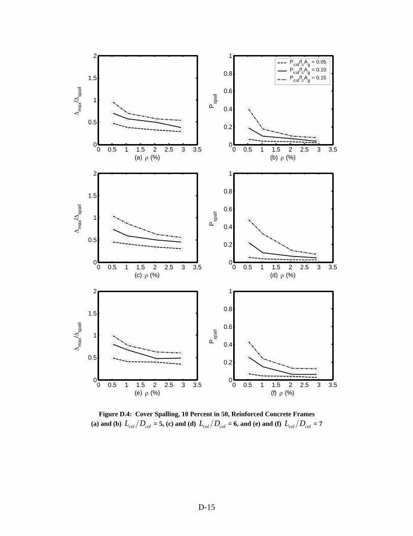
0 0.5 1 1.5 2 2.5 3 3.50
0.5
1
1.5
2
(a) ρ (%)
Δm
ax/ Δ
spal
l
0 0.5 1 1.5 2 2.5 3 3.50
0.5
1
1.5
2
(c) ρ (%)
Δm
ax/ Δ
spal
l
0 0.5 1 1.5 2 2.5 3 3.50
0.5
1
1.5
2
(e) ρ (%)
Δm
ax/ Δ
spal
l
0 0.5 1 1.5 2 2.5 3 3.50
0.2
0.4
0.6
0.8
1
(b) ρ (%)
Psp
all
Pcol/fcAg = 0.05Pcol/fcAg = 0.10Pcol/fcAg = 0.15
0 0.5 1 1.5 2 2.5 3 3.50
0.2
0.4
0.6
0.8
1
(d) ρ (%)
Psp
all
0 0.5 1 1.5 2 2.5 3 3.50
0.2
0.4
0.6
0.8
1
(f) ρ (%)
Psp
all
Figure D.4: Cover Spalling, 10 Percent in 50, Reinforced Concrete Frames (a) and (b) col colL D = 5, (c) and (d) col colL D = 6, and (e) and (f) col colL D = 7
D-15
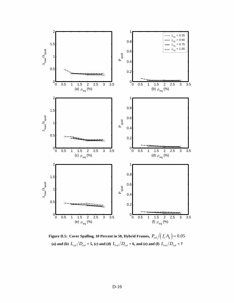
0 0.5 1 1.5 2 2.5 3 3.50
0.5
1
1.5
2
(a) ρeq (%)
Δm
ax/ Δ
spal
l
0 0.5 1 1.5 2 2.5 3 3.50
0.5
1
1.5
2
(c) ρeq (%)
Δm
ax/ Δ
spal
l
0 0.5 1 1.5 2 2.5 3 3.50
0.5
1
1.5
2
(e) ρeq (%)
Δm
ax/ Δ
spal
l
0 0.5 1 1.5 2 2.5 3 3.50
0.2
0.4
0.6
0.8
1
(b) ρeq (%)
Psp
all
λrc = 0.25λrc = 0.50λrc = 0.75λrc = 1.00
0 0.5 1 1.5 2 2.5 3 3.50
0.2
0.4
0.6
0.8
1
(d) ρeq (%)
Psp
all
0 0.5 1 1.5 2 2.5 3 3.50
0.2
0.4
0.6
0.8
1
(f) ρeq (%)
Psp
all
Figure D.5: Cover Spalling, 10 Percent in 50, Hybrid Frames, ( )' 0.05col c gP f A =
(a) and (b) col colL D = 5, (c) and (d) col colL D = 6, and (e) and (f) col colL D = 7
D-16
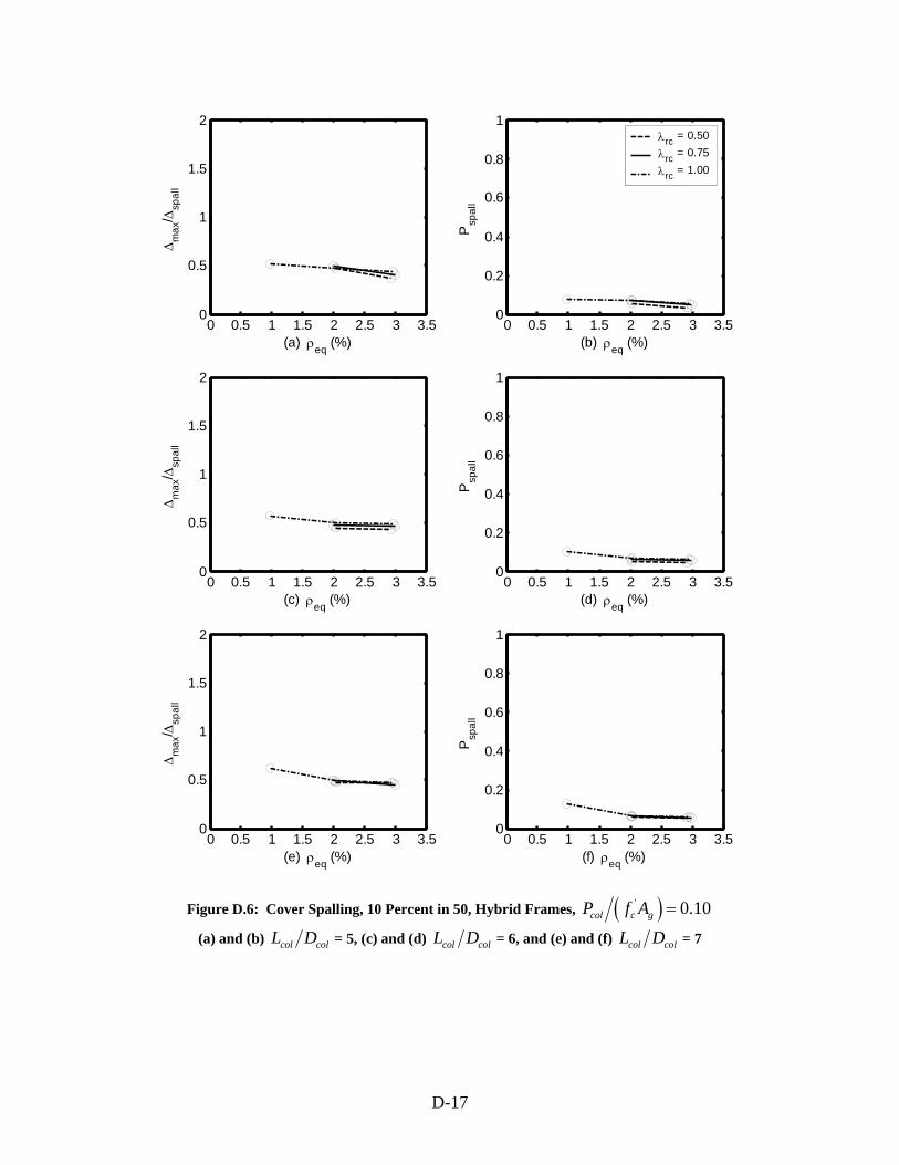
0 0.5 1 1.5 2 2.5 3 3.50
0.5
1
1.5
2
(a) ρeq (%)
Δm
ax/ Δ
spal
l
0 0.5 1 1.5 2 2.5 3 3.50
0.5
1
1.5
2
(c) ρeq (%)
Δm
ax/ Δ
spal
l
0 0.5 1 1.5 2 2.5 3 3.50
0.5
1
1.5
2
(e) ρeq (%)
Δm
ax/ Δ
spal
l
0 0.5 1 1.5 2 2.5 3 3.50
0.2
0.4
0.6
0.8
1
(b) ρeq (%)
Psp
all
λrc = 0.50λrc = 0.75λrc = 1.00
0 0.5 1 1.5 2 2.5 3 3.50
0.2
0.4
0.6
0.8
1
(d) ρeq (%)
Psp
all
0 0.5 1 1.5 2 2.5 3 3.50
0.2
0.4
0.6
0.8
1
(f) ρeq (%)
Psp
all
Figure D.6: Cover Spalling, 10 Percent in 50, Hybrid Frames, ( )' 0.10col c gP f A =
(a) and (b) col colL D = 5, (c) and (d) col colL D = 6, and (e) and (f) col colL D = 7
D-17
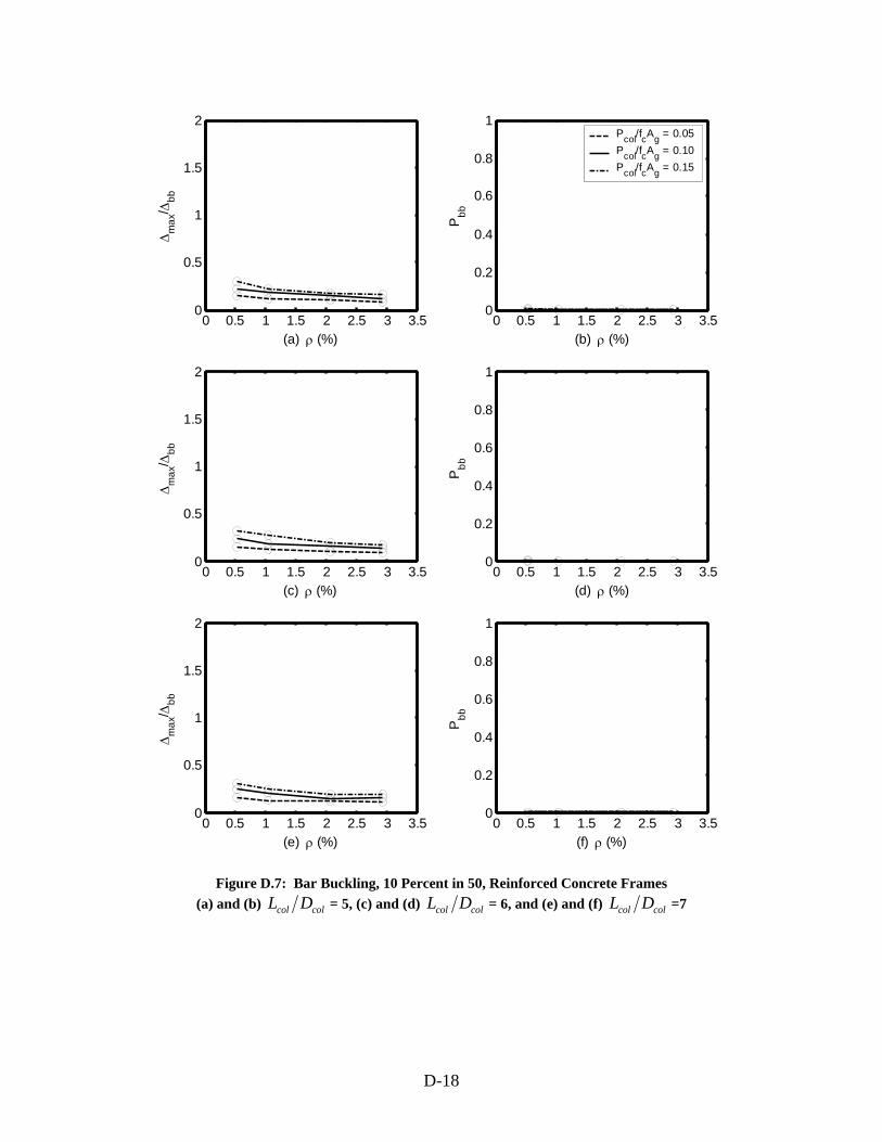
0 0.5 1 1.5 2 2.5 3 3.50
0.5
1
1.5
2
(a) ρ (%)
Δm
ax/ Δ
bb
0 0.5 1 1.5 2 2.5 3 3.50
0.5
1
1.5
2
(c) ρ (%)
Δm
ax/ Δ
bb
0 0.5 1 1.5 2 2.5 3 3.50
0.5
1
1.5
2
(e) ρ (%)
Δm
ax/ Δ
bb
0 0.5 1 1.5 2 2.5 3 3.50
0.2
0.4
0.6
0.8
1
(b) ρ (%)
Pbb
Pcol/fcAg = 0.05Pcol/fcAg = 0.10Pcol/fcAg = 0.15
0 0.5 1 1.5 2 2.5 3 3.50
0.2
0.4
0.6
0.8
1
(d) ρ (%)
Pbb
0 0.5 1 1.5 2 2.5 3 3.50
0.2
0.4
0.6
0.8
1
(f) ρ (%)
Pbb
Figure D.7: Bar Buckling, 10 Percent in 50, Reinforced Concrete Frames (a) and (b) col colL D = 5, (c) and (d) col colL D = 6, and (e) and (f) col colL D =7
D-18
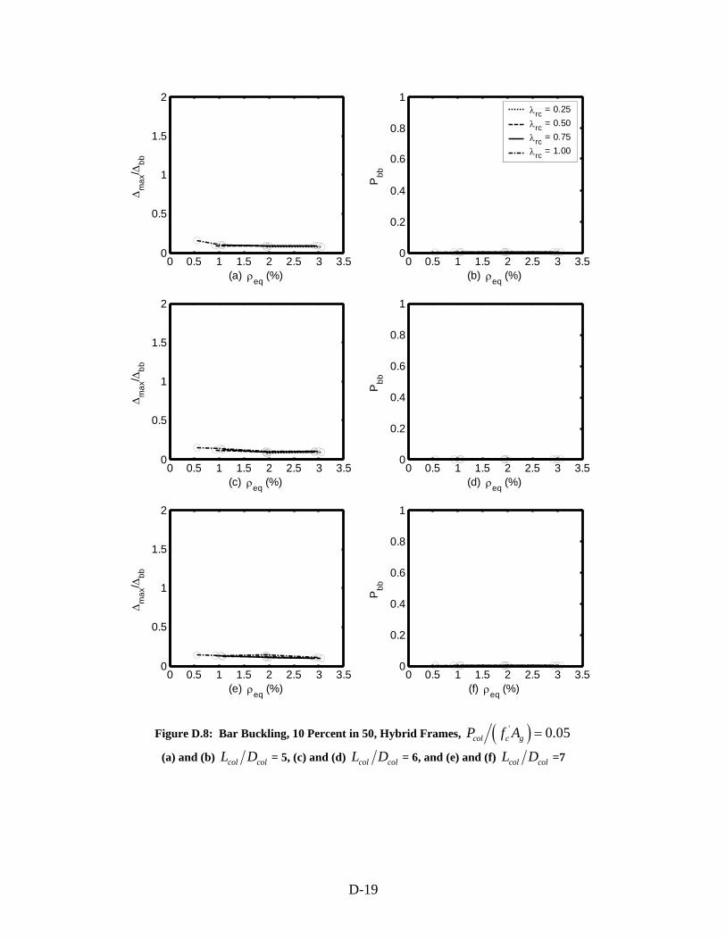
0 0.5 1 1.5 2 2.5 3 3.50
0.5
1
1.5
2
(a) ρeq (%)
Δm
ax/ Δ
bb
0 0.5 1 1.5 2 2.5 3 3.50
0.5
1
1.5
2
(c) ρeq (%)
Δm
ax/ Δ
bb
0 0.5 1 1.5 2 2.5 3 3.50
0.5
1
1.5
2
(e) ρeq (%)
Δm
ax/ Δ
bb
0 0.5 1 1.5 2 2.5 3 3.50
0.2
0.4
0.6
0.8
1
(b) ρeq (%)
Pbb
λrc = 0.25λrc = 0.50λrc = 0.75λrc = 1.00
0 0.5 1 1.5 2 2.5 3 3.50
0.2
0.4
0.6
0.8
1
(d) ρeq (%)
Pbb
0 0.5 1 1.5 2 2.5 3 3.50
0.2
0.4
0.6
0.8
1
(f) ρeq (%)
Pbb
Figure D.8: Bar Buckling, 10 Percent in 50, Hybrid Frames, ( )' 0.05col c gP f A =
(a) and (b) col colL D = 5, (c) and (d) col colL D = 6, and (e) and (f) col colL D =7
D-19
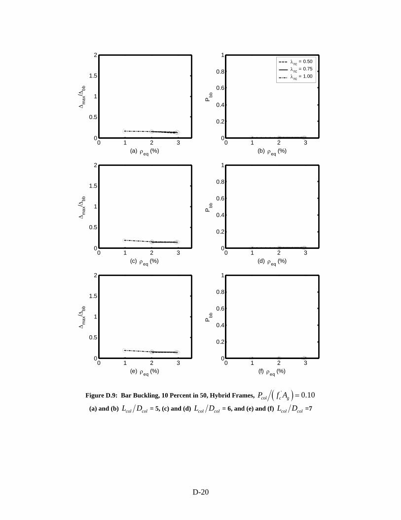
0 1 2 30
0.5
1
1.5
2
(a) ρeq (%)
Δm
ax/ Δ
bb
0 1 2 30
0.5
1
1.5
2
(c) ρeq (%)
Δm
ax/ Δ
bb
0 1 2 30
0.5
1
1.5
2
(e) ρeq (%)
Δm
ax/ Δ
bb
0 1 2 30
0.2
0.4
0.6
0.8
1
(b) ρeq (%)
Pbb
λrc = 0.50λrc = 0.75λrc = 1.00
0 1 2 30
0.2
0.4
0.6
0.8
1
(d) ρeq (%)
Pbb
0 1 2 30
0.2
0.4
0.6
0.8
1
(f) ρeq (%)
Pbb
Figure D.9: Bar Buckling, 10 Percent in 50, Hybrid Frames, ( )' 0.10col c gP f A =
(a) and (b) col colL D = 5, (c) and (d) col colL D = 6, and (e) and (f) col colL D =7
D-20
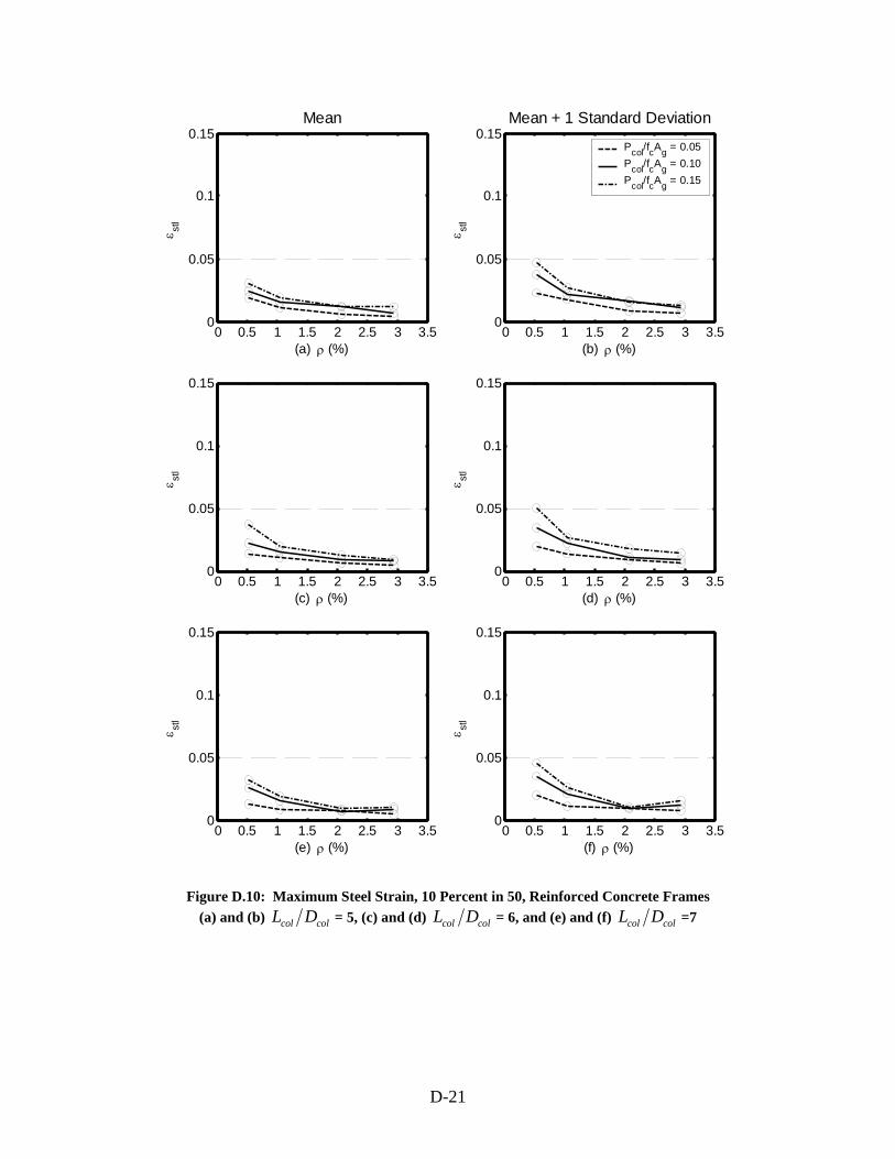
0 0.5 1 1.5 2 2.5 3 3.50
0.05
0.1
0.15
(a) ρ (%)
ε stl
Mean
0 0.5 1 1.5 2 2.5 3 3.50
0.05
0.1
0.15
(c) ρ (%)
ε stl
0 0.5 1 1.5 2 2.5 3 3.50
0.05
0.1
0.15
(e) ρ (%)
ε stl
0 0.5 1 1.5 2 2.5 3 3.50
0.05
0.1
0.15
(b) ρ (%)
ε stl
Mean + 1 Standard Deviation
Pcol/fcAg = 0.05Pcol/fcAg = 0.10Pcol/fcAg = 0.15
0 0.5 1 1.5 2 2.5 3 3.50
0.05
0.1
0.15
(d) ρ (%)
ε stl
0 0.5 1 1.5 2 2.5 3 3.50
0.05
0.1
0.15
(f) ρ (%)
ε stl
Figure D.10: Maximum Steel Strain, 10 Percent in 50, Reinforced Concrete Frames (a) and (b) col colL D = 5, (c) and (d) col colL D = 6, and (e) and (f) col colL D =7
D-21
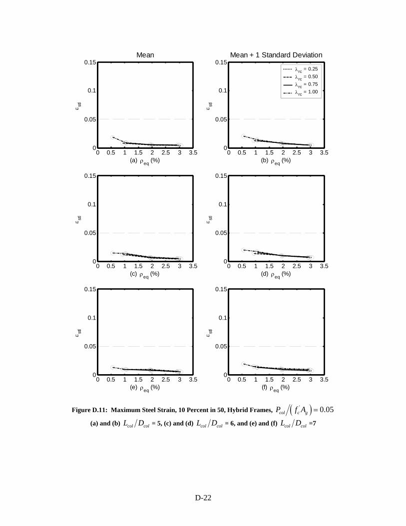
0 0.5 1 1.5 2 2.5 3 3.50
0.05
0.1
0.15
(a) ρeq (%)
ε stl
Mean
0 0.5 1 1.5 2 2.5 3 3.50
0.05
0.1
0.15
(c) ρeq (%)
ε stl
0 0.5 1 1.5 2 2.5 3 3.50
0.05
0.1
0.15
(e) ρeq (%)
ε stl
0 0.5 1 1.5 2 2.5 3 3.50
0.05
0.1
0.15
(b) ρeq (%)
ε stl
Mean + 1 Standard Deviation
λrc = 0.25λrc = 0.50λrc = 0.75λrc = 1.00
0 0.5 1 1.5 2 2.5 3 3.50
0.05
0.1
0.15
(d) ρeq (%)
ε stl
0 0.5 1 1.5 2 2.5 3 3.50
0.05
0.1
0.15
(f) ρeq (%)
ε stl
Figure D.11: Maximum Steel Strain, 10 Percent in 50, Hybrid Frames, ( )' 0.05col c gP f A =
(a) and (b) col colL D = 5, (c) and (d) col colL D = 6, and (e) and (f) col colL D =7
D-22
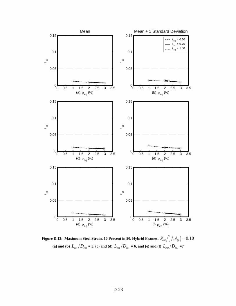
0 0.5 1 1.5 2 2.5 3 3.50
0.05
0.1
0.15
(a) ρeq (%)
ε stl
Mean
0 0.5 1 1.5 2 2.5 3 3.50
0.05
0.1
0.15
(c) ρeq (%)
ε stl
0 0.5 1 1.5 2 2.5 3 3.50
0.05
0.1
0.15
(e) ρeq (%)
ε stl
0 0.5 1 1.5 2 2.5 3 3.50
0.05
0.1
0.15
(b) ρeq (%)
ε stl
Mean + 1 Standard Deviation
λrc = 0.50λrc = 0.75λrc = 1.00
0 0.5 1 1.5 2 2.5 3 3.50
0.05
0.1
0.15
(d) ρeq (%)
ε stl
0 0.5 1 1.5 2 2.5 3 3.50
0.05
0.1
0.15
(f) ρeq (%)
ε stl
Figure D.12: Maximum Steel Strain, 10 Percent in 50, Hybrid Frames, ( )' 0.10col c gP f A =
(a) and (b) col colL D = 5, (c) and (d) col colL D = 6, and (e) and (f) col colL D =7
D-23
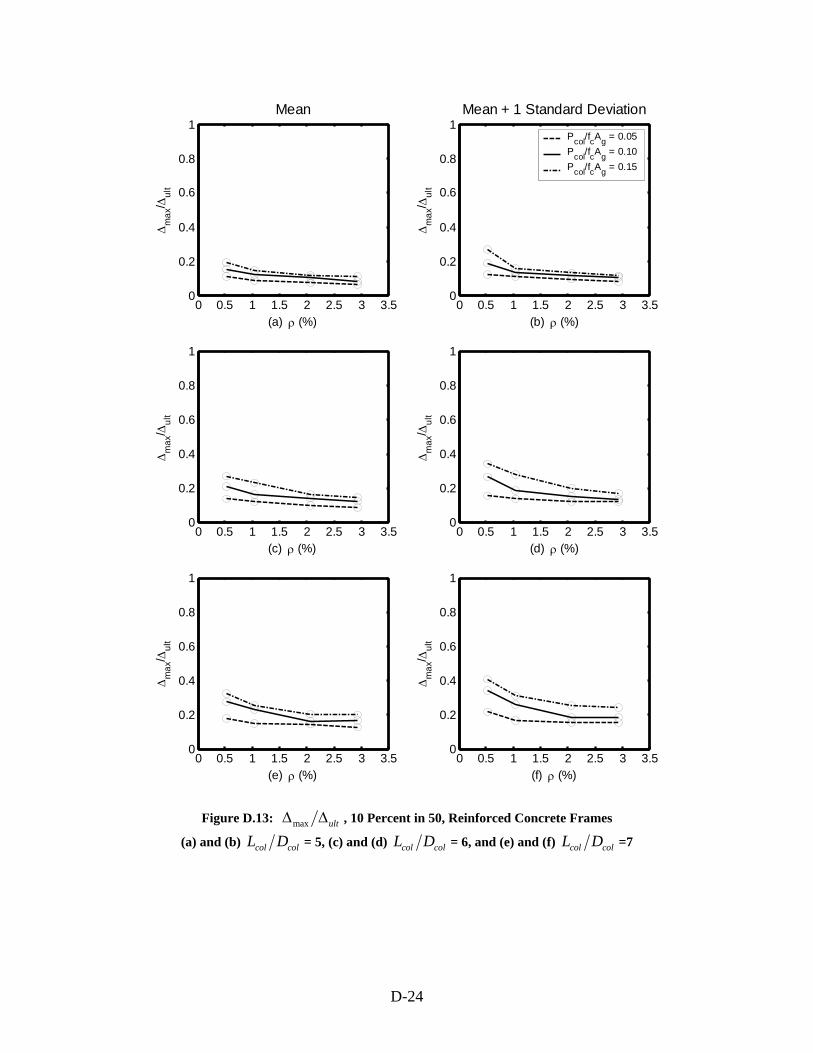
0 0.5 1 1.5 2 2.5 3 3.50
0.2
0.4
0.6
0.8
1
(a) ρ (%)
Δm
ax/ Δ
ult
Mean
0 0.5 1 1.5 2 2.5 3 3.50
0.2
0.4
0.6
0.8
1
(c) ρ (%)
Δm
ax/ Δ
ult
0 0.5 1 1.5 2 2.5 3 3.50
0.2
0.4
0.6
0.8
1
(e) ρ (%)
Δm
ax/ Δ
ult
0 0.5 1 1.5 2 2.5 3 3.50
0.2
0.4
0.6
0.8
1
(b) ρ (%)
Δm
ax/ Δ
ult
Mean + 1 Standard Deviation
Pcol/fcAg = 0.05Pcol/fcAg = 0.10Pcol/fcAg = 0.15
0 0.5 1 1.5 2 2.5 3 3.50
0.2
0.4
0.6
0.8
1
(d) ρ (%)
Δm
ax/ Δ
ult
0 0.5 1 1.5 2 2.5 3 3.50
0.2
0.4
0.6
0.8
1
(f) ρ (%)
Δm
ax/ Δ
ult
Figure D.13: max ultΔ Δ , 10 Percent in 50, Reinforced Concrete Frames
(a) and (b) col colL D = 5, (c) and (d) col colL D = 6, and (e) and (f) col colL D =7
D-24
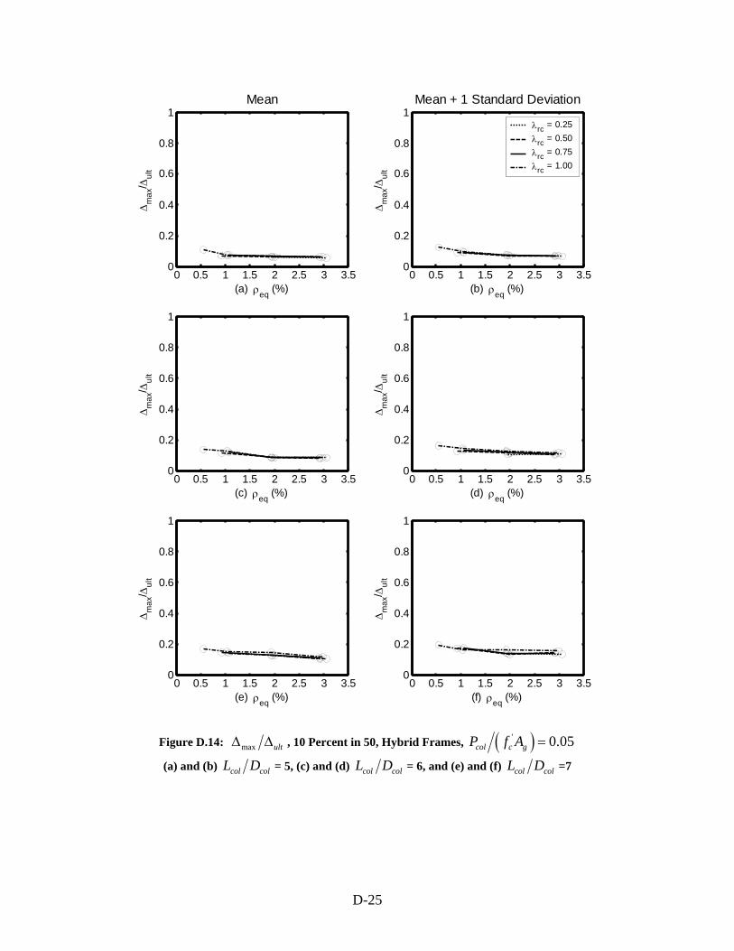
0 0.5 1 1.5 2 2.5 3 3.50
0.2
0.4
0.6
0.8
1
(a) ρeq (%)
Δm
ax/ Δ
ult
Mean
0 0.5 1 1.5 2 2.5 3 3.50
0.2
0.4
0.6
0.8
1
(c) ρeq (%)
Δm
ax/ Δ
ult
0 0.5 1 1.5 2 2.5 3 3.50
0.2
0.4
0.6
0.8
1
(e) ρeq (%)
Δm
ax/ Δ
ult
0 0.5 1 1.5 2 2.5 3 3.50
0.2
0.4
0.6
0.8
1
(b) ρeq (%)
Δm
ax/ Δ
ult
Mean + 1 Standard Deviation
λrc = 0.25λrc = 0.50λrc = 0.75λrc = 1.00
0 0.5 1 1.5 2 2.5 3 3.50
0.2
0.4
0.6
0.8
1
(d) ρeq (%)
Δm
ax/ Δ
ult
0 0.5 1 1.5 2 2.5 3 3.50
0.2
0.4
0.6
0.8
1
(f) ρeq (%)
Δm
ax/ Δ
ult
Figure D.14: max ultΔ Δ , 10 Percent in 50, Hybrid Frames, ( )' 0.05col c gP f A =
(a) and (b) col colL D = 5, (c) and (d) col colL D = 6, and (e) and (f) col colL D =7
D-25
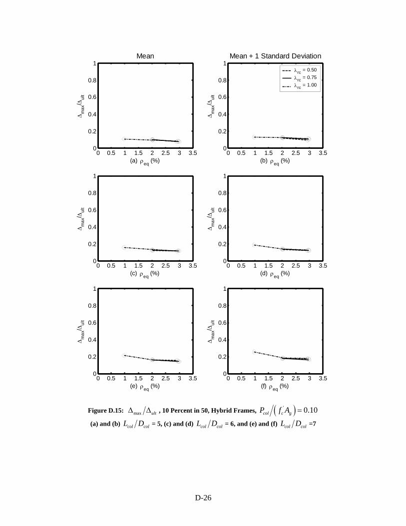
0 0.5 1 1.5 2 2.5 3 3.50
0.2
0.4
0.6
0.8
1
(a) ρeq (%)
Δm
ax/ Δ
ult
Mean
0 0.5 1 1.5 2 2.5 3 3.50
0.2
0.4
0.6
0.8
1
(c) ρeq (%)
Δm
ax/ Δ
ult
0 0.5 1 1.5 2 2.5 3 3.50
0.2
0.4
0.6
0.8
1
(e) ρeq (%)
Δm
ax/ Δ
ult
0 0.5 1 1.5 2 2.5 3 3.50
0.2
0.4
0.6
0.8
1
(b) ρeq (%)
Δm
ax/ Δ
ult
Mean + 1 Standard Deviation
λrc = 0.50λrc = 0.75λrc = 1.00
0 0.5 1 1.5 2 2.5 3 3.50
0.2
0.4
0.6
0.8
1
(d) ρeq (%)
Δm
ax/ Δ
ult
0 0.5 1 1.5 2 2.5 3 3.50
0.2
0.4
0.6
0.8
1
(f) ρeq (%)
Δm
ax/ Δ
ult
Figure D.15: max ultΔ Δ , 10 Percent in 50, Hybrid Frames, ( )' 0.10col c gP f A =
(a) and (b) col colL D = 5, (c) and (d) col colL D = 6, and (e) and (f) col colL D =7
D-26


![SECTION 034500 - PRECAST ARCHITECTURAL CONCRETE · Architectural precast concrete cladding [and load-bearing] units. ... PRECAST ARCHITECTURAL CONCRETE 034500 ... Architectural Cladding](https://img.pdfslide.net/doc/110x75/5ae006067f8b9a1c248cb77e/section-034500-precast-architectural-concrete-precast-concrete-cladding-and-load-bearing.jpg)