Precise Estimation of Elastic Moduli from Sonic Log Data ...demiller/2011_1IWRP_MillerHorneWalsh_presentation.pdf · Log Data from a Gas Shale Miller, Horne, Walsh, 1IWRP August 2011

Precise Estimation of Elastic Moduli from Sonic Log Data in a Gas Shale Formation

Douglas Miller1 Steve Horne2 John Walsh3

1st International Workshop in Rock Physics

10 August, 2011

1 Formerly Schlumberger, Cambridge MA; currently MIT EAPS and Miller Applied Science, LLC 2 Schlumberger, Fuchinobe, Japan 3 Schlumberger, Houston TX

Log Data from a Gas Shale

Miller, Horne, Walsh, 1IWRP August 2011

•  Standard dipole sonic acquisition & STC processing

•  Sonic data are from build section of deviated well

•  63% quartz; 35% clay; 2% calcite

Fit by a Single TI Model


Today’s Discussion

  Some background on anisotropy:   Phase, group, etc

  The Field Data •  Axial Moduli •  C13 and the Correspondence Rules •  Annie & other misfits

  The synthetic data & associated processing

  Concluding remarks


Sonic Log Data from a Gas Shale

400 pts from Vertical well

800 pts from Horizontal Section

800 pts from Build Section


•  Data from axial sections are summarized by histograms

•  Data from build section are plotted at borehole inclination angle

•  TI anisotropy, lateral and vertical homogeneity are evident from axial data


Fit by a Single TI Model

•  3DFD synthetics were created for 9 borehole orientations and 3 modes, then processed with STC

+ Processed 3DFD are plotted at borehole inclination angle

•  That’s 9000 data points fit with 5 parameters

•  We’ll describe how the model was obtained, and why it is of particular interest (beyond being a remarkable example of a match between data, in situ, and model).


An Important Point

•  There has been confusion in the literature regarding interpretation of sonic logs in deviated wells in anisotropic media. Because wavefronts radiated from a point source are not generally spherical, there has been uncertainty about whether borehole inclination should be matched to ray direction (group angle) or wavefront normal direction (phase angle).

Our data clearly show that, at least for fast anisotropic formations such as this gas shale, sonic logs measure group slowness for propagation with the group angle equal to the borehole inclination angle. The data are inconsistent with an interpretation that they measure phase slownesses for propagation with phase angle equal to borehole inclination angle.

The confusion in the literature stemmed from a failure to properly distinguish group slowness as a function of group angle from group slowness as a function of phase angle.


Phase and Group

•  Group direction points to source

•  Phase direction is normal to wavefront


Phase and Group

•  Wavefront expands without changing shape



•  Marked points have 55 degree group and phase angles respectively


Phase and Group






Phase and Group






Postma 1955

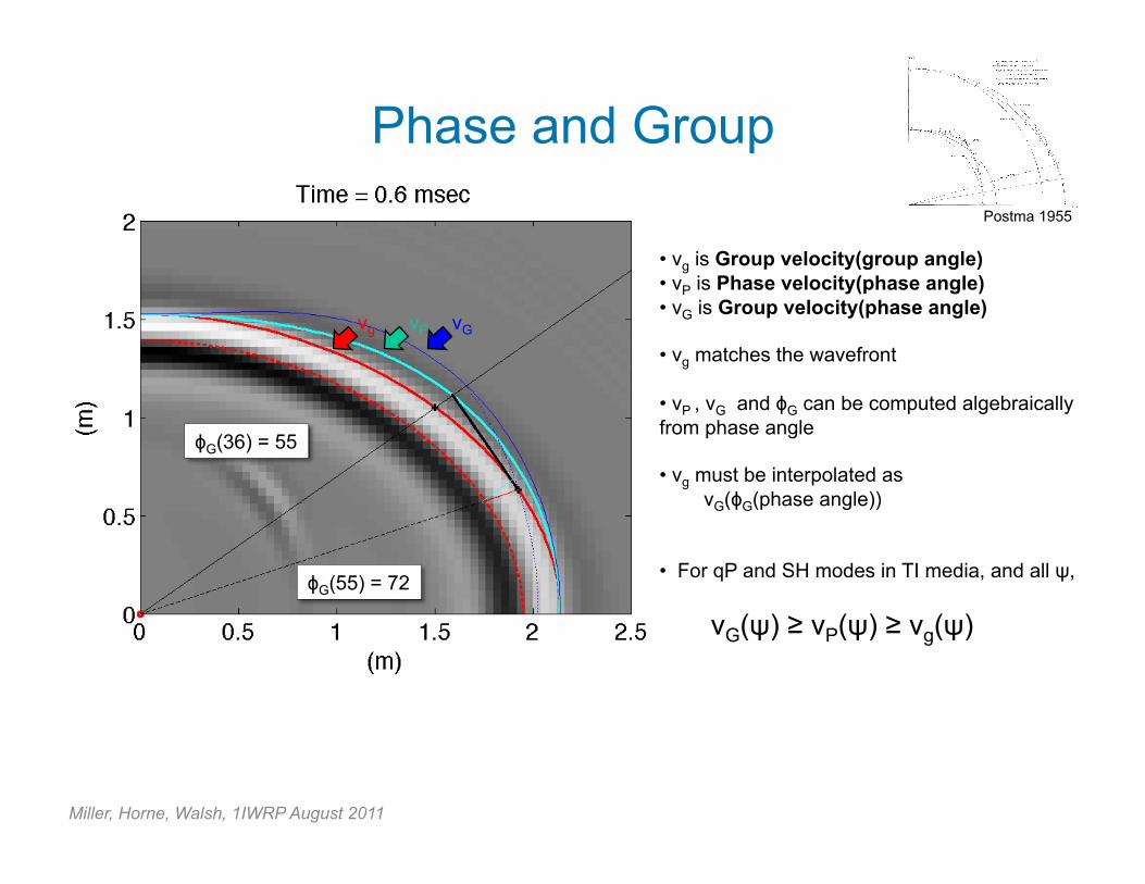
Phase and Group

vg vP vG

ϕG(55) = 72

•  vg is Group velocity(group angle) •  vP is Phase velocity(phase angle) •  vG is Group velocity(phase angle)

•  vg matches the wavefront

•  vP , vG and ϕG can be computed algebraically from phase angle

•  vg must be interpolated as vG(ϕG(phase angle))

•  For qP and SH modes in TI media, and all ψ,

vG(ψ) ≥ vP(ψ) ≥ vg(ψ)

ϕG(36) = 55


Sonic Log Data from a Gas Shale

400 pts from Vertical well

800 pts from Horizontal Section

800 pts from Build Section


•  Data from axial sections are summarized by histograms

•  Data from build section are plotted at borehole inclination angle

•  TI anisotropy, lateral and vertical homogeneity are evident from axial data


Four Moduli Directly from Axial Data

•  C13 remains to be found by a 1-parameter search

•  We need to know how C13 relates to off-axis log speeds (i.e. a Correspondence Rule)


Correspondence Rules: Hornby vs. Sinha

SEG Expanded Abstracts 2003 Do We Measure Phase Or Group Velocity With Dipole Sonic Tools? B. Hornby, X. WANG And K. Dodds

Comparisons of the computed velocities with the theoretical wave surfaces clearly shows the best fit with the group velocity surfaces. And so we conclude that we are measuring the group velocity for all wave modes excited by the dipole sonic tool.

Processing of synthetic waveforms in deviated wellbores using a conventional STC algorithm or a modified matrix pencil algorithm yields phase slownesses of the compressional and shear waves propagating in the nonprincipal directions of anisotropic formations.

GEOPHYSICS, 71(6) 2006 191–202 Elastic-wave propagation in deviated wells in anisotropic formations B. Sinha, E. Şimşek, and Q. Liu

The full-wave processing of dipole sonic logs using slowness time coherence has been demonstrated to yield phase rather than group velocities of compressional Vp and shear Vs waves (Sinha et al., 2006). This finding is imperative to the problem discussed in this paper because the angle dependence of phase and group velocities in anisotropic media can be quite different (Thomsen, 1986; Vernik and Liu, 1997).

- Vernik 2008, Geophysics


Correspondence Rules: Hornby and Sinha

(GG) Logs measure group slowness for propagation with the group angle equal to the borehole inclination angle (Hornby et al. 2003)

(PP) Logs measure phase slowness for propagation with the phase angle equal to the borehole inclination angle (Sinha et al. 2006)

When anisotropy is strongly present, these rules are incompatible. For the case at hand, (GG) is uniquely consistent with the data and matching synthetics. Sinha et al. reached their conclusion by confusing Hornby’s rule with a different one:

(GP) Logs measure group slowness for propagation with the phase angle equal to the borehole inclination angle (Sinha et al. 2006)

That is, Sinha et al. compared vP with vG rather than with vg.


SH Comparison

vg vP vG •  There are no adjustable parameters. Curves are determined by shear slownesses from horizontal well.

•  (GG) fits. (PP) and (GP) do not.

•  (GG) RMS misfit is .029 km/sec

•  (PP) RMS misfit is .082 km/sec


C13

vg vP vG •  Figures at left show RMS misfit as a function of C13 for (GG) in black, (PP) in gray.

•  (GG) fits both modes at C13 = 16.4 GPa

•  (PP) does not give a consistent answer

•  qSV best fit agrees with (GG) because, in this case, qSV phase and group surfaces are nearly coincident.

•  (PP) best fit for qP is physically unreasonable, -5 GPa.

qP

qSV


(GG) Best Fit

vP vg

•  vg in black, vP in gray, for each mode, using the (GG) best-fit value, C13 = 16.4 GPa

•  (GG) fits all modes

•  (PP) only fits qSV, (where phase and group surfaces happen to coincide).


(PP) Fit to qP Data

vP

•  vP in gray for each mode, using the value C13 = -5 Gpa, which fits the qP data with the phase surface.

•  qSV is egregiously misfit, with coincident shear speeds predicted at 55 degrees.

vP

vP


Best-Fit and 4-Parameter Approximations

δ = 0; C13 = C33 – 2 C55

δ = .1; C13 = -C66 + sqrt(C662 + C12 C33)

δ = .45; C13 = C11 – 2 C66

δ = ε=.48; C13 = sqrt(C11 – C55) (C33 – C55))

δ = .54; C13 = (C11 + C33)/2 – 2 C55

δ = .35; C13 = 16.4 GPa


Best-fit Parameters


3DFD

g P G

ϕG(72) = 55

•  Monopole source in fluid above an inclined half-space

•  Propagation in the solid matches the anisotropic wavefront surface, shedding a headwave.


3DFD

g P G

•  Monopole source in fluid-filled borehole

•  Wavefront in solid couples to reverberant “leaky P’ signal in borehole.

•  Signal in borehole slightly lags the wavefront in the solid.

vg vP vG


3DFD

•  Monopole source in fluid-filled borehole

•  Wavefront in solid couples to reverberant “leaky P’ signal in borehole.

•  Signal in borehole slightly lags the wavefront in the solid.


3DFD Processing

•  Waveforms and processing confirm what is evident in the snapshots

•  Semblance peaks are about 1% slower than 1/vg; 7% slower than 1/vP; 12% slower than 1/vG.

•  Temporal dispersion analysis using the Prony method yields a similar result. Temporal phase slowness at all frequencies is slower than 1/vg(ψbh)


Isotropic Example

•  Semblance peak is 2% slower than medium slowness


Bias Correction

•  The small bias between logged slowness and formation slowness is a feature of sonic logs that has always been present.

•  Processing all modes and angles in our synthetics, we found that a uniform 2% increase in elastic moduli gave an excellent match between semblance peaks and group slowness.


1)  Log data from this field example are remarkably consistent with the rule that sonic logs measure group slowness for propagation with the group angle equal to the borehole inclination angle. The data are inconsistent with an interpretation that they measure phase slownesses for propagation with phase angle equal to borehole inclination angle.

2)  Processed 3DFD synthetics simulating best-fit model confirm the interpretation.

3)  The best-fit model is close to satisfying the second Annie condition C13 = C12, as well as the elliptical condition, ε = δ.

4)  Data from deviated well alone would have been sufficient (but less convincing).

5)  See the extended abstract for more details. I’ll put a copy at www.mit.edu/~demiller

Concluding Remarks


•  Coauthors

•  Yang Zhang at MIT, Earth Resources Lab for help installing the 3DFD cone on my Mac mini

•  Phil Christie, David Johnson, Chris Chapman for helpful comments

•  The operating company for permission to show the data

Thanks to:

Documents

Precise Estimation of Elastic Moduli from Sonic Log Data ...demiller/2011_1IWRP_MillerHorneWalsh_presentation.pdf · Log Data from a Gas Shale Miller, Horne, Walsh, 1IWRP August 2011