Precision 3D Culvert User Manual

Release 1.1—March 9, 2015

• Imports DTMs from LandXML and Carlson TINS with texturing • Automatic Delineation of Watersheds • Computes Peak Flows by SCS and by Rational Methods • Automatically Sizes Culvert Pipes, both Circular and Rectangular • Illustrates Ponding Extents and Dewaters Ponds with Pipes • Storm Simulation with color coded Headwater Display • Inserts Headwalls from Extensive Headwall Library • All Design Conducted in 3D Environment • Designs can be augmented by 3D objects (trees, poles, buildings) • Pipe Systems can be Inserted by LandXML • Collision Analysis • Full PDF Reporting of Single or Multiple Storm Events • LandXML Exports to CAD for Plan and Profile Drafting

1

Table of Contents I. Program Layout and Structure ........................................................................................ 3

A. Installation ....................................................................................................................................... 3

B. Overview of Layout .......................................................................................................................... 4

C. Top Row Icons and Settings ............................................................................................................. 9

D. Pulldown Menus and Settings ....................................................................................................... 28

II. Loading DTMs, LandXML Surfaces and Scenes (entire P3D Projects) .............................. 43

A. Loading Carlson DTM Surfaces with Texturing (TIN and LandXML) .............................................. 43

B. Polylines and Applications for Texturing and Station/Skew Angle ................................................ 46

C. Saving and Loading Scenes ............................................................................................................ 51

III. Watershed Delineation and Peak Flow Calculation ........................................................ 53

A. Calculating Watershed Boundaries ................................................................................................ 53

B. Tooltips and Subcatchment Information ....................................................................................... 55

C. Peak Flow by SCS Method and by Rational Method (Q=CIA) ........................................................ 58 D. Pond Display, Stream Display and Controls ................................................................................... 60

IV. Culvert and Headwall Placement .................................................................................. 63

A. Placing, Editing, Moving, and Locking Culverts .............................................................................. 63

B. Pipe Calculation Examples ............................................................................................................. 66 C. Visual Indicators ............................................................................................................................. 93

D. Inserting, Editing, and Designing Headwalls .................................................................................. 95

E. Scenario Cost Calculation ............................................................................................................... 97

V. PDF Reporting and Exporting to CAD ............................................................................. 99

A. PDF Reports on Culverts and Watersheds ..................................................................................... 99

B. Exporting Plan, Profile, Pipe Networks, and Revised DTM Data to CAD ..................................... 101

VI. 3D Object Insertion ..................................................................................................... 104

A. Inserting 3D Objects ..................................................................................................................... 104 B. Expanding the 3D Object Library ................................................................................................. 105

C. Animating Objects ........................................................................................................................ 106

VII. LandXML Files ............................................................................................................ 108

A. Importing LandXML Files ............................................................................................................. 108 B. Exporting LandXML Surfaces, Pipe Networks, and Hydrology Data ............................................ 108

VIII. System/Program Performance .................................................................................... 110

A. Required/Recommended Hardware ............................................................................................ 110

B. Ways to Improve Speed ............................................................................................................... 110 C. Time Tests .................................................................................................................................... 117

2

I. Program Layout and Structure A. Installation

Precision 3D Culverts and the entire Precision 3D Series requires a 64-bit processor running Windows 7 or higher. The above screen appears when these conditions are met, during install. You can select Intellicad, Autocad or install the software stand alone. If installed stand alone, the software goes by default to the Carlson Precision 3D subdirectory as shown below:

If installed on Intellicad or Autocad®, it installs in the directory of the CAD engine. In the case of Intellicad 8.0, for example, it installs to: C:\Program Files\Carlson2015_ICAD8_X64. In all installations, a compiler is installed as well, producing the new screen icon shown below:

3

It sets up automatically that data files recalled by the program go in the directory: C:\ProgramData\Carlson Software\Precision3DCulverts\Data inside which the following subdirectories appear:

B. Overview of Layout Precision 3D is organized as shown below. The icons on top are command categories for distinct applications like loading surfaces or placing culverts within the routine. On the left side, the Scene Explorer shows a tree of all work activity and provides additional commands within the major, distinct command options. The 3D graphics appear in the middle of the screen and to the right are Tooltips that illustrate parameters and values as you mouse over key hydrologic or graphic features. The pulldown menus on top provide alternate ways to initiate the commands or features of the Scene Explorer and also include additional commands such as Settings.

4

The Scene Explorer column on the left is further divided into an initial “tree” zone in the upper left which records all commands and operations and organizes them by category such as surface “TIN” file, Storm Event, Culvert and Headwall insertion, Object insertion, etc. Multiple scenarios can be created each containing multiple storm events and other features. Below that is the Property Explorer which allows for parameter, design element and settings changes. There is also a tab for placing of textures to enhance the screen viewing. An Output zone appears in the lower left, and records all activity and is particularly useful as an indicator that calculation processes are done. At the very bottom left of the screen, the coordinates of the mouse position are presented at all times, including real-time elevation feedback as you move the mouse. Your active surface file is also displayed for reference. The Tooltips appear on the right side of the screen, which always include coordinates at the top right and below that, data on screen elements appears as you mouse across the 3D site. If you hover over a pond, for example, pond volume, area and maximum depth appears. Lighting control appears at the bottom right of the screen. As you move the sun closer to the horizon or edge of the circle, the shading becomes more intense and more contrast is obtained. Dockable dialogs: The various components of the screen (Scene Explorer, Property Explorer, Output, Tooltips and the Lighting Control) are movable. At installation, Output may occupy the entire lower area, but can be gripped and moved to occupy just the lower left as shown above. The lighting control area can be reduced in size or even removed leaving more room for the

5

Tool Tip information. You can always click on the Tools pulldown menu and select Light Settings to adjust them, leaving the entire right column for the Tooltips. Placing the sun near the horizon leads to more contrast and shadows, and intensity can be adjusted.

During the design process, if the cursor is placed inside a watershed, you will see the drainage area (in the case below, 4.879 acres) and the peak flow and all the parameters used in the calculation. Furthermore, if the cursor is placed over a ponding area, you will also see pond information in the Tooltips at right, including maximum pond depth and volume of water.

To undock any docked window (Scene Explorer, Tooltip, Output, etc...), place the mouse cursor on the top most dialog menu bar, then left mouse click - holding down the mouse button and drag the window away from the frame. The dialog will resize to undocked size and may be placed anywhere on the screen, inside or outside of the main application window. Below is the Tooltip information gripped and moved to a new free-floating position. Note that the Light Control then expands to the entire zone on the right. If the Tooltips are moved upward, they will take on a full screen horizontal appearance at the top of the page. But such a

6

position would be a poor use of screen space since the data in the Tooltips is arranged in a columnar format. For the free-floating position shown, place the Tooltips low enough that they don’t “snap” to the top of the screen, then expand upwards by moving the mouse over the top and obtaining the expand grips:

To dock a window to the main application window, place the mouse cursor on the top most dialog menu bar, then left mouse click - holding down the mouse button and drag the window towards the main application window edges. As the mouse approaches the top, left, bottom or right, a shaded preview rectangle will automatically appear to indicate where the window will dock when the left mouse button is released. If an existing window is already in a docked area, dragging a window to that same region will show a shaded preview rectangle and dragging the window up/down or left right will allow docking above or below the existing docked window.

7

Moving the Output window to the left (see below) will allow left frame docking under or above the existing docked windows.

To hide or make any window visible, use the View menu option. Checked window names are visible, unchecked windows are hidden.

8

The overall effect is a rich and dynamic design environment where the display of textured 3D surfaces, ponds and flowing water reveal the impacts of hydrologic design decisions and guide the user quickly to workable solutions.

C. Top Row Icons and Settings Load Surface

The “Load Surface” icon is highlighted above. If you place the cursor over this icon, the “Load Surface” tooltip will appear. You can also choose Load Surface by using the “Right Click” of the mouse, which brings up all major commands. Left Click to select the command from the list.

9

When Load Surface is selected, the following dialog appears, allowing selection of the TIN surface (triangulated network surface). Click browse (3 dots) to select TIN plus grid or LandXML surfaces (first LandXML surface found will load):

If the surface is in meters (which has a significant impact on drainage calculations), be sure to click that option above. The last setting (feet or meters) will be remembered. Surface data can be placed anywhere, but you can also make use of the default directory shown below (Program Installed Location\Data\Surfaces).

Scenarios: Under the File pulldown, there is an option to Add Scenario. If you want to load more than one surface (even if one is in metric and the other in feet), you should place the new surface in a new Scenario. You can switch between them by selecting the desired surface in the Scene Explorer “tree” shown at left:

10

When a surface is highlighted, a green bounding box is drawn around the surface to indicate it is selected. Whenever other objects are selected and “active”, such as culvert pipes or headwalls, they are also highlighted by a green bounding box. Carlson TIN Files and Auto-Texturing: The Carlson Civil program has the ability to make a TIN file with color attributes for each triangle in the TIN. These colors are then “mapped” to textures automatically by Precision 3D Culverts. In this way, TIN surfaces appear with more clarity. Road and shoulder surfaces, as well as cut and fill slopes and embankment dams are distinctly colored and then intelligently textured within Precision 3D Culverts. The commands RoadNet, Pad Template, Valley Pond and Bench Pond all have this built-in coloring capability when making the output surfaces. When these TIN surfaces are brought into Precision 3D Culverts, they immediately appear as multi-textured surfaces as shown below:

You can also drag and drop a new texture to replace any existing textures, as shown below:

The actual default mapping of texture is set under the Tools pulldown menu, Texture Map tab:

11

Surfaces do not have to be Carlson TIN files (.tin extension). They can also be Carlson Grid files (.grd extension) or can be generic LandXML surfaces made in other software packages. You would click the LandXML icon to load these LandXML TIN files. However, the current LandXML 1.0 does not permit association of colors with triangles. Therefore, at loading, only one texture can be applied to the surface. However, using the polyline icon, a closed perimeter can be drawn and distinctly textured to distinguish surface land cover types. The new LandXML 2.0, which is due to be produced in late 2015, will offer coloring of TIN triangles and will allow for auto-texturing of surfaces similar to the loading of Carlson TIN files. Surface Viewing Controls: Once surfaces are loaded, they position themselves by default in the center of the screen as shown below:

The Background Color is user-defined, under Tools pulldown, Settings, System Tab:

12

The first thing to do is to hold the left button of the mouse down and do a forward motion of the mouse which pulls the site closer to the horizon and brings the sky into view.

Then roll the mouse wheel forward to zoom in. Hold the mouse wheel down to pan in any direction. Holding the left mouse button down, move the mouse left and right to “spin” the site in the desired direction. Double click the left mouse button to zoom in at your clicked location. Use Ctrl Double click of the left mouse button to zoom out. Double click on the surface file in the Scene Explorer to zoom extents, restoring the original 3D View.

Contours: If you click on and select the loaded surface, you can scroll down through the Property Explorer and turn on Contours. Contours will plot at any set interval, with index contours automatically shown at 5 times the chosen interval. The contours just add to the program visually, but are not exported.

13

Place Culvert

The Place Culvert command requires that a surface be loaded first. Typically, you would compute the subwatersheds and peak flows in each subwatershed using the Calculate Storm Event icon, prior to placing culverts. This Calculate Storm Event icon appears below. In the Scene Explorer, you must highlight the Active Storm Event (and set the desired storm parameters), at which point you obtain the Calculate Storm Event icon shown below.

After a short computation (longer if the terrain model is very large), all areas of ponding as well as major stream courses are displayed graphically, and culverts can be placed with the purpose of draining and dewatering these ponds. Little vertical yellow “sticks” indicate low points, and when placing culverts, the upstream inlet position will automatically “snap” to these low points when the cursor is moved close to them. If no storm event has been calculated, a default discharge (in English units) of 10 cfs (cubic feet per second) is assumed. This value can be changed during the act of placing a culvert by clicking the inlet position of the culvert, then moving the cursor left to the Property Explorer that appears for the culvert, where you can real-time adjust the flow to a different number.

14

So if you know the flow of the water to be drained, you can bypass the Calculate Storm Event procedure and place the culvert by directly entering the desired flow to discharge.If the Calculation Mode is set to CalcPipeSzie, then once a pipe has been placed, you can change the discharge or allowable design headwater depth and the pipe will automatically re-size.

The Calculation Mode can also be set to Calculate Headwater and Calculate Discharge. In the Calculate Headwater mode, the culvert pipe diameter and discharge values can be changed, and a new headwater elevation is calculated. Similarly, in Calculate Discharge mode, the pipe diameter and headwater can be changed resulting in a new discharge calculation. In Place Culvert, the pipe always will rest on the ground. During the placement process, if the pipe is running uphill, it will appear yellow, both in the 3D view and in the Property Explorer next to Pipe slope:

15

This changes to green (good), when the pipe slope is downhill (negative). The pipe takes on its normal gray coloring when drawn downhill. It is orange if design parameters are exceeded.

Pipes can be “locked” so no design process changes them. The lock icon is an action icon that locks the pipe when clicked. This icon appears gray during the design process, when it is not accessible. Once placed, the invert elevations of the pipe inlet and outlet can be adjusted. Placing Culverts to Drain Ponds: Most culvert design is done after a storm event has been calculated and peak flows are computed by the program, rather than hand-entered as above. Following “Calculate Storm Event”, ponding occurs in all low areas, and culverts can then be sized to drain the ponds at the accepted inlet headwater. Shown below are 2 ponding areas in a 2” rainfall event, as calculated by the SCS method (CN=65):

The above pond calculation is obtained by clicking on a Storm Event (or right-clicking to Add a Storm Event while highlighting and existing Storm Event) and changing the rainfall to 2” as shown. Then click the Calculate Storm Event icon highlighted above in the lower left. Note that the Max Depth of water in the middle pond (obtained by hovering mouse over that pond)

16

is 7.28’. When a culvert pipe is placed to drain the upper embankment, the pond to the right, the water will drain to the middle pond and increase its depth, as shown below:

Maximum depth of the middle pond is now 8.173’, the pond having risen nearly 1 foot after receiving the water from the upper pond above the embankment dam. The upper pond has been drained effectively. Note also that the pipe slope, length and invert elevation is displayed at left, following placement of the pipe. The magenta perimeters indicate the maximum storage capacity of each pond up to the lowest point of overflow, and helps advise on impacts from flooding.

In a close-up view of the ponding effects, you can see that Pond 2 has risen, but not yet to the elevation of Pond 3, which is a higher “perched” pond to its left. At the overflow point indicated by the upward arrow, Pond 3 first drains to Pond 2 until water rises to a common level, at which point it fills and overflows at the point indicated by the left-arrow above. Precision 3D Culverts, by precisely modeling water flow on the surface provided, will reveal pond and stream behavior graphically based on any number of specified storm event and pipe design scenarios. Pipe culverts can be rectangular and circular. Circular culverts can be drawn as concrete material or as corrugated metal pipes. In addition to single pipes of a certain size, multiple barrels of pipes can be designed, in which case the pipe dimensions are reduced as appropriate to handle the design flows. The pipe inlet and outlet can be gripped and moved to new locations at any time.

17

The Place Culvert command is described more fully in Chapter IV, Culvert and Headwall Placement. Insert Headwall

After a pipe culvert has been placed, the Insert Headwall command can be used to apply a headwall to both ends of the culvert pipe. Rules are available to push the headwall into the hill, which reduces the pipe length and cuts out earthwork around the headwall. Then when the pipe is gripped and moved, the original surface model is restored and the process can be repeated at a new invert location.

Shown above is a headwall placed on a pipe, prior to selecting the option to “Auto-Design” the headwall into the hill according to grading rules. Headwalls cans be selected from an extensive headwall library. Once headwalls are placed they appear in the tree. Select the outlet headwall as shown, and then use the icon below to grade the headwall into the hill:

Here is another headwall shown after the Auto-Design is selected. It pushes into the hill leaving the user-defined “freeboard” from the top of the headwall against the hill down to the earth.

18

Insert Headwall mimics the real-world by reducing pipe lengths to what would be installed whenever headwalls are involved. With headwalls in place, culvert commands such as 2 barrels (versus the default 1 barrel) can be used and the appropriate pipe re-sizing and solid modeling will occur, as shown below:

Auto Create Culvert

The Auto Create Culvert icon is in effect a combination of the Place Culvert icon and the Place Headwall icon. It accomplishes both processes in one step. You get a pipe and headwalls. Immediately after placing the pipe, you are prompted for your headwall selection. Shown below is the result of Auto Create Culvert using an elongated style of headwall.

19

If you grip on the cyan square for the selected Culvert Pipe, you can move the culvert pipe to a new position. In its final position, if you highlight the Outlet headwall object in the tree, you can click on the “Auto Design Headwall” icon and push the headwall into the hill to the desired minimum freeboard, reducing the pipe length and duplicating field installation conditions. Note how the pipe length reduces from 145.553’ above to 120.319’ below.

Turn “Show Grading Polyline” to “False” to hide white grading lines.

20

Load LandXML

The Load LandXML command can be used for 2 main purposes:

(1) To bring in surface LandXML files in the form of TIN files allowing specific selection of the TIN file component to use, if multiple surfaces exist in the LandXML file.

(2) To bring in existing storm and sanitary sewer systems that have been stored in LandXML format, in order to test for collisions.

The opening dialog appears below, and in this case, an existing sanitary sewer system in LandXML format is selected:

Transparency and Viewing Collisions: The plot of this system is shown below, as it interferes with a newly designed pipe. You can view the pipes through the surface by setting Transparency “True” and something like 0.75. To do this, click into the surface in the tree in the upper left, choose the Display tab and locate these transparency options. Restore to Transparency “False” when done. Note that the Culvert 3 design pipe appears in red because a decision has been detected with the imported LandXML sanitary sewers.

21

If a LandXML file is loaded that contains 2 or more surface, you obtain all the files in the tree, and can delete immediately the surfaces you don’t want to use, isolating to the target surface.

Items in the Scene Explorer tree can be deleted by selecting them and pressing the Delete key or right clicking and selecting Delete. Load 3D Model

You can load 3D Models from the Precision 3D Library of objects, which includes a variety of features such as trees, light poles, vehicles and other objects that add realism to the design.

22

You begin by selecting objects from the available libraries. For example, if you choose the tree category, the tree objects appear and you can scroll through them and select the one you prefer:

These objects can then be placed on the surface at any picked location. Here are trees, light poles and guardrail as well as a survey tripod as placed near the road above the ponds

If you highlight Sub-basins, you can turn off (set False) “Show Areas”, and if you highlight Ponds, you can turn off“Show Outlines” for a less cluttered graphic. Whenever objects are inserted, they can be placed vertically or perpendicular to the surface.

23

Culvert Pipe Report

Precision 3D Culverts will produce a PDF Report on any selected pipe culvert. First, select the culvert to report by locating it in the Scene Explorer tree. Then click on PDF Report.

Select the desired report. The standard Culvert Pipe Report Form fills out 2 pages worth of data for the selected pipe. The first page is shown below:

24

Draw Polyline

The Draw Polyline icon is used for 2 primary purposes:

(1) To draw a closed perimeter inside which texturing can be applied (2) To create a horizontal alignment for purposes of computing pipe skew angles

For example, if a certain area has a very distinct ground cover, this can be represented by a specific texture. So you could first draw a polyline around the target perimeter and then place

25

a texture inside. You do not need to remove textures that are there already. The latest texture will simply override what occupies the perimeter of the new texture. After Clicking Draw Polyline, use the right mouse button to pick each vertex of the new polyline and press C on the keyboard to close to the beginning point. Then click the Texture tab in Scene Explorer, choose your category and select your texture within the category. To indicate rip-rap or stone in a steep drainage channel, you might click as shown:

Then use a “drag and drop” motion to pull the texture over to the right and drop it inside the perimeter. If the scale of the texture is too large, adjust by tapping the Polyline and highlighting it, then going to the Display tab and increasing the resolution for a smaller scaled hatch pattern:

26

The second major application of the Draw Polyline command is to create a horizontal alignment that can be used to compute the skew angle of the selected pipe. First select the alignment and then when producing the PDF Report, you will be asked to select the target pipe. The KY PDF report, for example, has a place holder for skew angle:

Measure Distance

This is a very useful command for evaluating distance and slope between any two points. For example, if we had an area of stone rip-rap in a steep drainage channel, we could measure that area by picking the 2 endpoints to determine its length and slope. Press Esc to exit Measure.

27

D. Pulldown Menus and Settings File Pulldown Menu

Open Scene: A Scene is everything under the Scene Explorer, everything in the tree of commands and objects shown below:

So when you Save Scene, you save all the information of the design including the surface, the texturing and the design aspects. Open Scene recalls any previously saved Scene. Add Scenario: The design process often involves many scenarios. You may take one pipe design but apply different storm event scenarios to it. You may have two surfaces that you wish to test in two different scenarios on the same storm event. You may want to simply distinguish your design by time, referring back to a previous design effort as a distinct scenario. The option Add Scenario allows you to set up a new scenario that can contain any number of commands, design decisions, textures and objects. Load Surface: This command in the File pulldown is identical to the Load Surface command which is the first icon at the top of the screen, described in detail earlier and in Chapter II. It allows you to select a Carlson TIN, a Carlson Grid file or a LandXML file containing a surface. The surface is then placed in 3D view in the graphic window of Precision 3D.

28

Save to CAD: This takes a current snapshot of the design work and created a LandXML file that can be loaded in any CAD program, such as Intellicad 8.0, Autocad ® and Civil 3D ® and Microstation ®. These programs have LandXML import commands that will detect the design features in the LandXML, as shown below in the Carlson LandXML import command using Intellicad 8.0 as the CAD platform:

You then select which elements of the LandXML you wish to import. The pipes and headwalls will draw as solids within Carlson and the surfaces will draw as a triangular mesh. Save Scene: This command saves all aspects of the Scene as recorded in the Scene Explorer. Scenes including the design surface, pipe designs, watershed data and special 3D objects can then be shared and loaded by others. Import: This command will bring in Wavefront objects and Sketchup “.skp” files and plot these objects directly to the screen. You simply search for the appropriate file. In this case, we are are selecting a fire hydrant “sketchup” formatted “.skp” file:

Then you pick a point on the surface to place the object.

29

Export Scene: There are 3 Export options: Wavefront (.obj), Stl and 3D Printer. The entire scene can be saved as a “.obj” surface. Many programs read “.obj” files, including Solid Works and Autodesk 3D Studio. 3D Printing: The Stl export and 3D Printer export are both provided to enable 3D Printing.

P3D provides 3D printing preparation and export to .STL files for the surfaces and objects in the current scenario. The export feature will create a series of cubes based on the number of rows and columns entered in the export dialog. To create the 3D print ready files, select the menu option File->Export Scene->3D Printer.A dialog prompt specifies the output file directory to create or use and the base file name for the STL files. The number of rows is the number of vertical divisions and the columns specify the number of horizontal divisions.

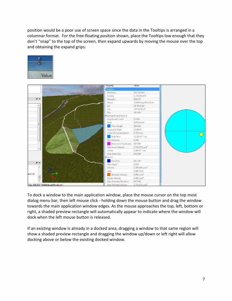
A 2x2 grid will produce a total of 4 STL files each representing a single cube. The files will be exported to the specified directory using the base file name entered plus it’s cube or cell number. In this example will produce the following output files:

30

Here are the 4 scene files re-assembled in Blender:

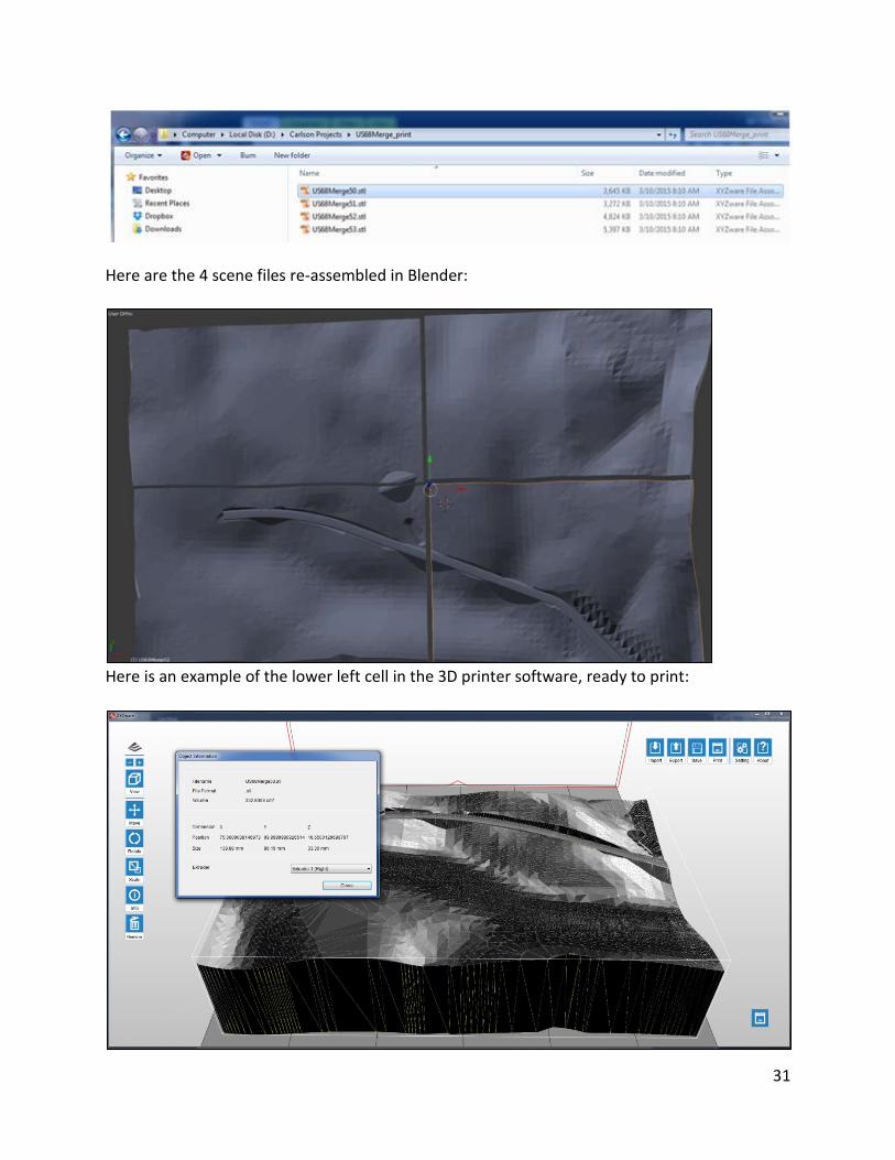
Here is an example of the lower left cell in the 3D printer software, ready to print:

31

The smaller 3D Printers can be purchased for as little as $1000 or less, and larger 3D Printers are available at higher cost. They can be very useful in making scale models of proposed designs, and with multi-colored cartridges, they can produce color-coded models as shown below:

Edit Pulldown Menu The Edit Pulldown Menu has just 2 options, Undo and Redo.

The Undo command undoes your last action and will keep going stepwise undoing previous actions. The Redo command will restore your last action only.

32

View Pulldown Menu

The View Pulldown Menu allows you to turn off and on any aspect of the screen “zones” that you don’t consider necessary for your work environment. In case you move an area off the screen and lose track of it, the View Pulldown Menu also allows you to restore it. The Off-On controls are intelligent in that the program remembers the last position of the screen element in question. If you have Light Control and Tool Tips tabbed together in the same column as shown below, turning off Light Control leads to only Tool Tips on the right side, for example. This is a useful option, since Tools has the option to review Light Control in a separate command, making the instant access Light Control less critical.

33

Tools Pulldown Menu The Tools Menu has 2 options: Light Settings and Settings. Light Settings has an important option to set Ambient Intensity. This should be set to a middle level, typically, to obatin sufficient contrast. A high light intensity is recommended. Placing the light near the edge of the sky circle (near the horizon) creates more shadows and also can improve viewing.

34

The embankment dam at left lacks visible edges at the top of the dam with 100% Ambient Intensity, but with a lower Ambient Intensity as set above, the edges of the dam come back into view. The Settings option contains a multi-tab set of Settings. For correct Latitude and Longitude, choose your correct projection. Projection Types include UTM zones.

The main “System” settings are shown below:

35

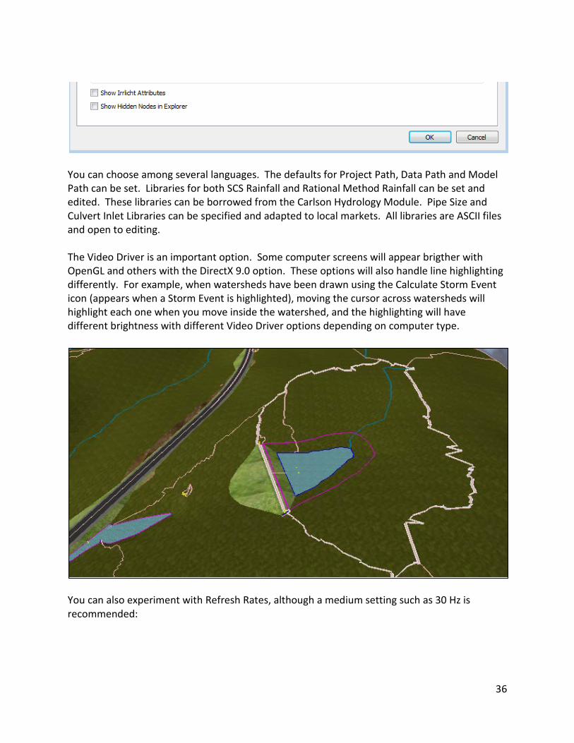
You can choose among several languages. The defaults for Project Path, Data Path and Model Path can be set. Libraries for both SCS Rainfall and Rational Method Rainfall can be set and edited. These libraries can be borrowed from the Carlson Hydrology Module. Pipe Size and Culvert Inlet Libraries can be specified and adapted to local markets. All libraries are ASCII files and open to editing. The Video Driver is an important option. Some computer screens will appear brigther with OpenGL and others with the DirectX 9.0 option. These options will also handle line highlighting differently. For example, when watersheds have been drawn using the Calculate Storm Event icon (appears when a Storm Event is highlighted), moving the cursor across watersheds will highlight each one when you move inside the watershed, and the highlighting will have different brightness with different Video Driver options depending on computer type.

You can also experiment with Refresh Rates, although a medium setting such as 30 Hz is recommended:

36

The Z Far setting of 10000 is recommended. The background color is the color below the sky and below the surface itself. The following zone of settings can have a far-ranging effect on speed and viewability and should be selected carefully:

Showing Moving Water is a “safe” setting having little effect on speed, but adding a lot to the impression of the water. Water will “flow” and move in ponds and in streams, particularly when you zoom in close. This setting does not tap resources.

If you turn on “Show Water Reflections”, this will begin to draw upon resources. Ponds will reflect the sky above. The most demanding on resources is Show Shadows, which also has 3 control settings beneath it. With this option on, the graphics may not react to mouse movement as quickly, but surface objects will project shadows and if set to DirectX, ponds will display transparency allowing viewing of the surface beneath the water. (Show Moving Water is on).

37

If Show Multi-Textured Surfaces is turned off, the site reverts to a single default texture:

The “Show Rip-Rap Texture” option will automatically place rip-rap at the outlets to headwalls, with dimensions defined in the headwall placement. “Show Runoff Tracking Values” will present flow rates and flow volumes along streams below pipe culverts at the bottom of the screen (see below). Just mouse over the streams to see these values. Add these flow rates to the peak flow from the culvert pipe calculation, and you have total flows that help you design open channel dimensions and select channel lining.

38

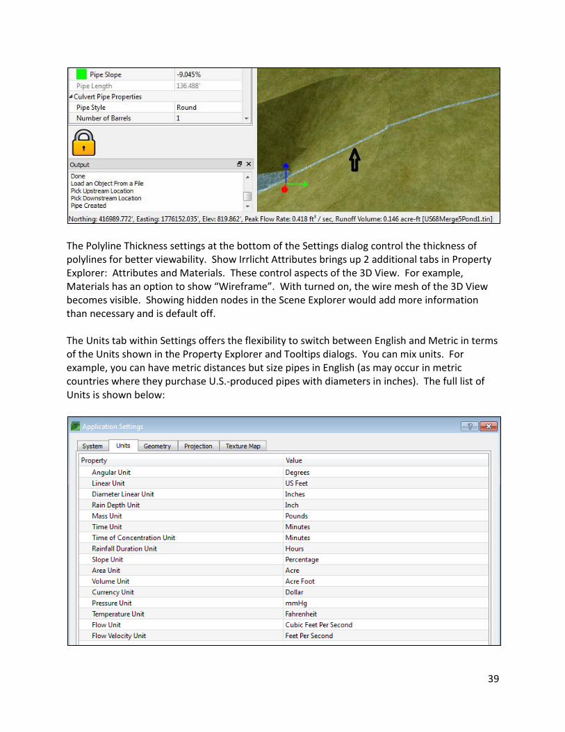
The Polyline Thickness settings at the bottom of the Settings dialog control the thickness of polylines for better viewability. Show Irrlicht Attributes brings up 2 additional tabs in Property Explorer: Attributes and Materials. These control aspects of the 3D View. For example, Materials has an option to show “Wireframe”. With turned on, the wire mesh of the 3D View becomes visible. Showing hidden nodes in the Scene Explorer would add more information than necessary and is default off. The Units tab within Settings offers the flexibility to switch between English and Metric in terms of the Units shown in the Property Explorer and Tooltips dialogs. You can mix units. For example, you can have metric distances but size pipes in English (as may occur in metric countries where they purchase U.S.-produced pipes with diameters in inches). The full list of Units is shown below:

39

The Geometry tab of the Application Settings is shown here:

It has just a few options governing display of 2D Polylines for things like watershed boundaries. The Projection tab was discussed earlier. The Texture Map tab offers many controls for viewing textures:

The default Texture File for each selected color is set at right. The Texture Resolution may need to be adjusted for any selected default texture, to create the best appearance in the 3D view. The Default Color to Texture Mapping column at left allows you to add more colors and associated textures, in case the TIN files being loaded have a greater variety of color than shown. At the bottom of the Texture Map screen is a + and – button to add more color mapping or to remove colors that are mapped. Sometimes, due to TIN editing in CAD or other functions, you may lose the colors of a certain area on the textured surface or have unwanted colors:

40

Just right click over the area in question and select Change Texture:

A similar texture is Ground type, “Just Add Bison” (odd sounding texture). This will blend in this area more closely with the surrounding texture:

You can right click over any particular mapped texture on the site to see its current texture setting and scale.

41

Commands Pulldown Menu This menu allows for selecting of commands also found in the icons.

Utilities Pulldown Menu This menu currently offers the Measure Utility, with operation identical to the icon “Measure”. Help Pulldown Menu This menu offers Help, which shows the product name and build date. The initial Release 1.1 has a build date of March 9, 2015. The Registration option within Help shows your serial number and status (registered or demo).

42

II. Loading DTMs, LandXML Surfaces and Scenes (entire P3D Projects)

As previously mentioned, Precision 3D Culverts allows you to use three types of Digital Terrain Models: Carlson TIN files (.tin), Carlson Grid files (.grd), and LandXML files (.xml). These surfaces can be imported to Precision 3D using the Load Surface Icon, or by Right Clicking and selecting Load Surface. You will see a dialog box which allows you browse for the surface file. It is important to note that surfaces are expected to be in English coordinates with units of feet. Therefore, it is import to select the Surface in Meters checkbox if your surface uses metric coordinates. When a surface is imported, it will be brought into the active Scenario. If you would like to import multiple surfaces, it is recommended that you use different Scenarios for each surface. To create a new Scenario, click the File Pulldown Menu > Add Scenario. You can then double click the Scenario to make it active. You can change the way a surface appears by using the Property Explorer. For detailed information, see Section I Part C of this document.

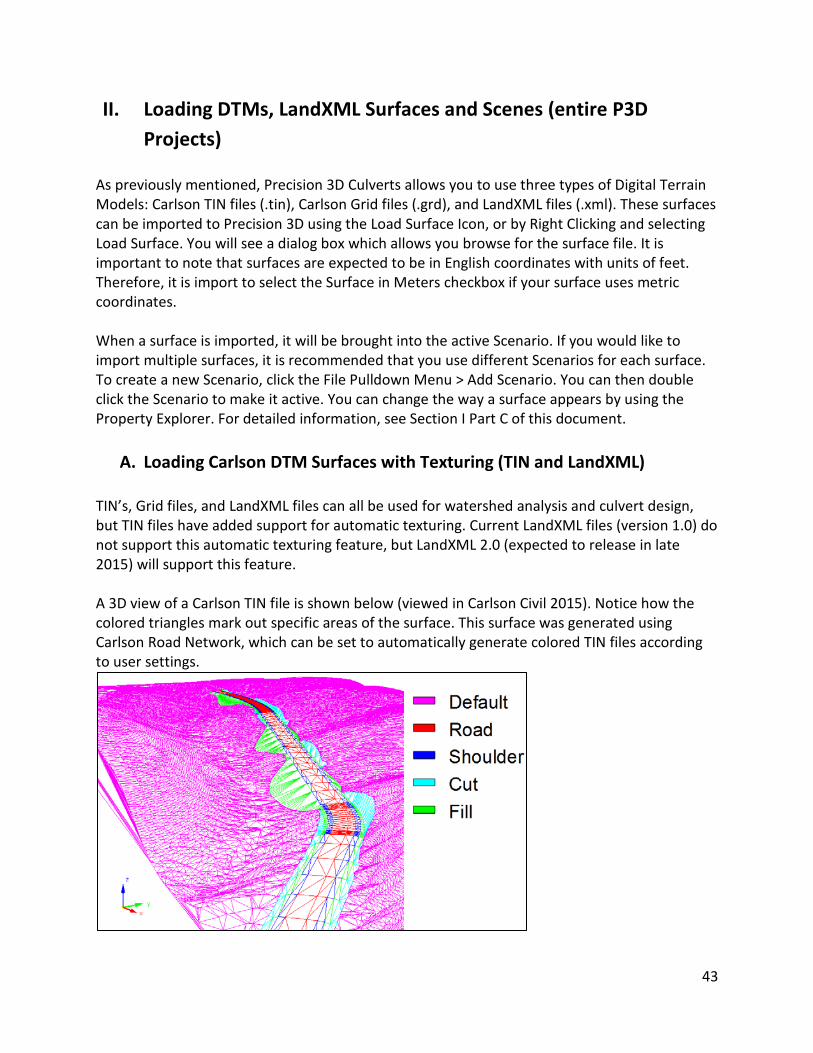
A. Loading Carlson DTM Surfaces with Texturing (TIN and LandXML) TIN’s, Grid files, and LandXML files can all be used for watershed analysis and culvert design, but TIN files have added support for automatic texturing. Current LandXML files (version 1.0) do not support this automatic texturing feature, but LandXML 2.0 (expected to release in late 2015) will support this feature. A 3D view of a Carlson TIN file is shown below (viewed in Carlson Civil 2015). Notice how the colored triangles mark out specific areas of the surface. This surface was generated using Carlson Road Network, which can be set to automatically generate colored TIN files according to user settings.

43

TIN files can also be colored manually using Triangulation File Utilities within Carlson Civil 2015. To color a TIN file, you must first draw a closed polyline around the area to be colored. You can then use Triangulation File Utilities (Found under Carlson Civil 2015 Module > Surface Pulldown Menu > Triangulation File Utilities) to load the TIN surface and select the inclusion line to mark the area to be colored. In the below picture, the surface has been loaded into Triangulation File Utilities and the bounding polyline has been selected. Notice how the triangles within the bounding polyline are highlighted in green, indicating that only these triangles will be affected by the next action. The ‘Set Color’ button can then be used to assign a color to the highlighted triangles. The surface can then be saved to a new TIN file (be sure to select all three checkboxes under “Output Options” to ensure you save the entire surface to the new file).

Notice that after the manual edit, the triangles included in the bounding polyline have been set to an orange color, whereas they were previously green.

44

With the TIN File edited, it can be brought into Precision 3D and textures can be applied to each of the various TIN colors. The Tolls Pulldown Menu > Settings > Texture Map tab will bring up the dialog shown below. Here we have added the new orange color to match that of the manual edit shown above. Notice that colors are input in Red-Green-Blue (RGB) format, which is named when selecting the triangle color in CAD. With the color set, an image can be applied to the color by clicking the ellipse next to Texture File. This will allow you to select a texture image from the included library, or you may select your own.

Once the color has been added and a texture has been ‘mapped’ to that color, the change will be reflected in the Graphics Window, as shown below. If you would like to texture a scene without making manual edits to the TIN file, you can use closed polylines to mark out areas for texturing. This is discussed in the following section.

45

B. Polylines and Applications for Texturing and Station/Skew Angle Polylines can be added to the scenario for 3D object animation, texturing areas, station and angle referencing for culverts, and simply marking out areas of interest. Clicking the icon shown to the right will start the command. Simply pick the points for the line to follow and press ‘Enter’ to end the command. Alternatively, you can right-click to pick the final point on the line, or press ‘C’ to close the polyline.

Once drawn, a new group will be created in the Scene Explorer, which lists all polylines that have been drawn using this command. You can edit the name of the polyline to make identification easier by right-clicking on the polyline name. The polyline color can also be edited by clicking the button to the right of “Line Color” in the Property Explorer. Polylines can be turned on and off by toggling the “Visibility” option under the Display tab in the Property Explorer.

46

Polylines can be drawn in the horizontal plane at a fixed elevation or they can be draped onto the surface. By default, polylines are draped onto the active surface, but can be reassigned to drape to another surface in the Property Explorer. You can also edit the polyline to be drawn at a fixed elevation. The default elevation can be edited by clicking Tools Pulldown Menu > Settings > Geometry Tab, and is shown in the below picture. In this menu the “Height Above Surface” refers to the highest point on the surface. For example, using the default value of 5.00 would draw a 2D polyline 5.00 feet/meters above the highest point on the surface.

Closed polylines can be used to texture specific areas. In the below picture, the closed polyline has been drawn around the outflow of the pipe to mark the new stream area. This area can be textured to show that it will be different from the original ground. To change the texture, click on the Texture Tab next to the Property Explorer, select a texture, and drag-and-drop it into the closed polyline area. The texture can also be changed by right-clicking inside the closed polyline area. Right-clicking to edit will also allow you to change the texture resolution, which is defined as number of images per unit area; the higher the value, the smaller the size of the individual texture image.

47

Polylines can also be used to report skew angles and station referencing for culverts. In the below picture, the road centerline has been drawn in orange, and has been assigned as the reference polyline for the culvert.

48

A visual explanation of the reported values is shown below. The skew angle (shown in magenta) is reported as the angle between the pipe and the direction perpendicular to the reference line. The stationing (shown in red) is reported as if the inlet and outlet were projected onto the reference line. The offset of the inlet and outlet (shown in cyan) is given as the perpendicular distance from the reference line to the respective point.

49

Polylines can also be used for animation of 3D Objects. For detailed information about objection animation, see Section VI Part C of this document.

50

C. Saving and Loading Scenes Projects within Precision 3D Culverts can be saved and later re-opened to further analyze and edit your design. To save a scene, click the File Pulldown Menu > Save Scene. This will create a .3dp file in the directory you specify. The .3dp file type is simply a zipped folder with a different file extension. This allows you to move the .3dp file between various machines, and even to other users without having to reference the original files. You can actually rename the file extension to that of a zipped folder to see the individual files contained within the scene. For example, the file ‘My_Scene.3dp’ could be renamed to ‘My_Scene.zip’, which would change the file type to a standard zipped folder. This folder contains images used to texture the scene, the original surface file, the updated surface file, a LandXML file containing polyline information, a zipped folder containing the headwall files, and more depending on your specific project.

51

Scenes can also be saved to a format intended for 3D Printing. This does not, however, allow you to open the scene again for further watershed analysis. For detailed information about saving Scenes to these formats, see Section I Part D of this document. To open a saved Scene, simply click the File Pulldown Menu > Open Scene. Here it is important to note the difference between a Scene and a Scenario. A Scenario contains a surface file, polylines, culverts, headwalls, 3D objects, etc. to be used for watershed analysis. A Scene is a collection of Scenarios. A Scene can be saved, but individual Scenarios cannot. You can only open one Scene at a time.

52

III. Watershed Delineation and Peak Flow Calculation A. Calculating Watershed Boundaries

When a surface TIN or LandXML surface is loaded, the program immediately highlights the Storm Event as shown below. When this is highlighted, you can click Calculate Storm Event in the lower left, which uses all the parameters set in the Property Explorer for the Storm Event. Storms can be defined by the SCS method or by the Rational Method.

So the procedure at start-up is a two-step process of loading your Surface (verifying your settings and storm parameters) and then clicking on the Lightning Bolt icon shown above, to Calculate Storm Event. If you have worked other commands in the meantime, you will need to click on and highlight the Storm Event (1 or higher number in different Scenario) which brings up the Calculate Storm Event icon. Click this icon to calculate the watershed boundaries.

The program outlines all watersheds and subwatersheds. A watershed, like the one shown above, is a self-contained area where the water does not overflow or leave the watershed in the prescribed storm event. When you move the cursor into the watershed, you see all the

53

major hydrologic information such as longest flow length, average land slope, time of concentration and peak flow. If you hover over any ponds shown, you will also see maximum pond depth and pond volumes. But in areas where basins fill and overflow, the subwatersheds are automatically combined into the largest watershed that doesn’t exceed two conditions under Property Explorer:

(1) Cutoff Area (2) Maximum Pond to Merge

So if the water pools in what amounts to a large puddle, you don’t want to consider that as a separate watershed. Very few TIN surface files are so exact that you won’t have some small low areas even with the best of design tools. So the program will “ignore puddles” in effect, by combining small pond volumes up to a Maximum value, above which the pond will be isolated as a distinct watershed. Small areas or volumes of water are ignored and connected to larger watersheds. Using these 2 settings, a roadside ditch with little puddles or tiny basins will therefore avoid creation of excessive watershed areas needing their own special culverts for drainage. Gate Technology: Even if watersheds are combined by the program, you have the ability to isolate watersheds using the Gate Icons.

Blue as shown above indicates that water is flowing through the gate by natural processes. This is the normal setting when a gate between subwatershed appears. You can click on the gate and change it to Green, which forces the water to flow through and automatically links what otherwise could be separate watersheds, or to Red, which stops the water from flowing through for calculation and design purposes, isolating your study to the volume of water and peak flow above the gate. Each time a gate is changed, to see its effect on the watershed calculation, it is important to click the icon Calculate Storm Event.

54

Since the program makes a decision whether to link watersheds based on size and volume of dammed up water, these Gates provide control to force a linked watershed (upper to lower) or block a linked watershed. If the water from the storm doesn’t pool up sufficiently to create a gate, then no gate will appear.

B. Tooltips and Subcatchment Information The right side of the screen offers “Tooltips” when moving the cursor across a site. If a drainage area that the program internally isolates is joined to the lower area by a green gate, the cursor in the position shown below might reveal a higher Peak Flow and drainage area, considering what is above and below the gate. Peak flow here is 7.04 cfs and the drainage area is 19.055 acres.

But if this same area is gated off with a red gate, as the program may have internally done on its own, the cursor in that same position shows only the upper subwatershed data on the right:

55

Peak flow is now 3.73 cfs from a subwatershed area of 9.841 acres. When you move the cursor over a pond, you see in addition the maximum pond depth and all pond data, at the bottom of the Tooltip on the right:

Here, the maximum depth of this pond is shown as 10.12 feet, volume 0.3 acre feet. This would be more than a “puddle”—you need to place a culvert to drain this pond, ideally with the upstream invert at the low point indicated by the yellow stick. Bear in mind that these yellow sticks may be submerged. You can turn off the blue pond water by selecting Ponds in the Scene Explorer, then going to the Display tab in Property Explorer and turning off Show Ponds:

56

By doing this, we discover a still lower point in the “double pond” shown above (2 low points). Subcatchment information will be drawn back to CAD in the form of a LandXML file that will import into nearly all CAD software. This subcatchment information is useful by itself, separate from the added value gained when culverts are designed and exported to CAD. First, you need to enter Precision 3D from CAD, using Carlson Civil Suite (any module) in Autocad or Intellicad or using Carlson Simplicity in Microstation. Then be sure to “Save to CAD” under the File pulldown menu after watersheds are drawn in Precision 3D Culverts. Then return to CAD and the watersheds will plot (some watershed boundaries below are gripped to reveal their perimeters):

Everything is layerized for selective freezing and thawing, including the watershed and pond data shown below:

57

C. Peak Flow by SCS Method and by Rational Method (Q=CIA) SCS Method Rainfall: If the SCS Method is chosen, rainfall is defined very simply as a depth in inches or millimeters (or the unit depth specified under Tools > Settings). TR-20 is used. Time of Concentration is computed from the curve number, average land slope and length of flow.

Rational Method Rainfall: If the Rational Method is selected (click to the right of Hydro Method to see SCS and Rational options), various rainfall libraries can be chosen from which to calculate your rainfall amount based off of the return period and in some cases the rainfall duration. Each library can contain many storm types, which contain rainfall information specific to the site. The location of the rainfall library can be specified in Settings, and can actually be recalled from the Carlson Hydrology library location (default c:\carlson projects\settings):

Once a rainfall library has been set, you can choose between the various storm events included in the library. This can be done by clicking to the right of Rational Storm Type in the Property Explorer as shown below:

58

Libraries can be edited/created to fit your site via the Carlson Hydrology Module by simply inputting collected rainfall data using one of seven methods shown below.

This information is used to calculate the Intensity-Duration-Frequency (IDF) Curve coefficients, which are used to calculate the rainfall amount for a given return period and in some cases the storm duration. For more information on editing and creating storm events using the Carlson Hydrology Module, please see the Carlson Software 2015 Manual > Hydrology Module > Network Menu > Rational Rainfall Library, which can be found under the Help Pulldown Menu in any Carlson Module or online at http://files.carlsonsw.com/mirror/manuals/Carlson_2015/index.html. An example of how you might set up a rainfall library is shown below. The Ohio DOT uses a single rainfall library containing four storm types – each one corresponding to a specific region in the state. The rainfall library as it would be seen in the Carlson Hydrology Module is shown below. Notice that each storm type was created by manually entering the IDF Equation coefficients, and that the Rainfall ID is the same as a Rational Rainfall Storm Type in Precision 3D.

59

The below picture shows the information contained in the Ohio-A storm type. Here we have the three IDF coefficients listed for six return periods.

In Precision 3D, the rainfall library is used to calculate the effects of the various storm events. As the Rainfall Return Period rises from, say, 10 year to 50 year to 100 year, a higher rainfall intensity is calculated, leading to a greater Peak Flow. Each calculated Rainfall Return Period used will appear on page 2 of the standard Culvert Report, so this report can include multiple Rainfall Return events. Runoff can be calculated by Universal, Dekalb or Modified Rational Methods. As previously mentioned, the rainfall amount is interpolated from the rainfall libraries for a given return period and rainfall duration. However, the rainfall duration is automatically calculated when the Dekalb or Universal Methods are used. This value is defined as 10*Tc for the Dekalb Method and 11*Tc for the Universal Method.

D. Pond Display, Stream Display and Controls Ponds are drawn automatically in low points when Calculate Storm Event is clicked. The water surface is drawn to the extent water would be collected and impounded by the storm, based on ground cover (curve numbers and runoff coefficients) and rainfall depth or intensity. This water extent is drawn by a dark blue line. The magenta line indicates the maximum headwater level before overflow out of the basin would occur. The cyan polyline is the longest flow line in length. The thick white perimeter is the watershed itself, which may include some component pink subwatersheds.

60

Water in the pond can be drawn as solid blue, a motion-based blue (as above) or a sky-reflecting blue. These settings are found within Tools, Settings, System Tab:

The individual indicator lines for headwater can be turned off and on using the Display tab, with Ponds selected in Scene Explorer:

61

Streams: Moving the cursor across the site, after Calculate Storm Event has been clicked, will reveal the flow rates at that point on the natural surface. If you move the cursor along a flow line stream, you can see the increasing flow from the right position (shown first below) to the position where the stream enters the pond:

First, a peak flow rate of 0.021 cfs on the right-side of the above screen, and then just as the stream enters the pond, the flow rate has increased to 0.75 cfs.

Note that flow enters the pond not just from the longest flow line but from all directions surrounding the blue pond perimeter inclusive of the pond itself. Total Peak Flow in this example, entering the pond, is 1.915 cfs with the selected storm event.

62

IV. Culvert and Headwall Placement Once you have calculated the storm events of interest, watershed boundaries and ponds will be shown in the Graphics Window. By placing culverts, you can dynamically drain these ponds and effectively direct flow to lower ponds.

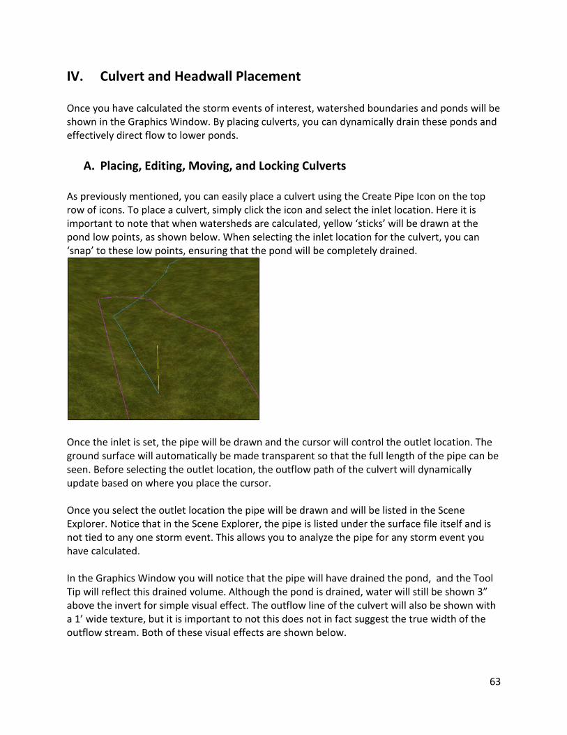
A. Placing, Editing, Moving, and Locking Culverts As previously mentioned, you can easily place a culvert using the Create Pipe Icon on the top row of icons. To place a culvert, simply click the icon and select the inlet location. Here it is important to note that when watersheds are calculated, yellow ‘sticks’ will be drawn at the pond low points, as shown below. When selecting the inlet location for the culvert, you can ‘snap’ to these low points, ensuring that the pond will be completely drained.

Once the inlet is set, the pipe will be drawn and the cursor will control the outlet location. The ground surface will automatically be made transparent so that the full length of the pipe can be seen. Before selecting the outlet location, the outflow path of the culvert will dynamically update based on where you place the cursor. Once you select the outlet location the pipe will be drawn and will be listed in the Scene Explorer. Notice that in the Scene Explorer, the pipe is listed under the surface file itself and is not tied to any one storm event. This allows you to analyze the pipe for any storm event you have calculated. In the Graphics Window you will notice that the pipe will have drained the pond, and the Tool Tip will reflect this drained volume. Although the pond is drained, water will still be shown 3” above the invert for simple visual effect. The outflow line of the culvert will also be shown with a 1’ wide texture, but it is important to not this does not in fact suggest the true width of the outflow stream. Both of these visual effects are shown below.

63

Once placed, pipes can be moved by selecting the pipe and dragging-and-dropping the blue grip shown at the outlet and the inlet location. The grip is shown below.

64

The pipe properties will be listed in both the Tool Tip and the Properties Explorer, as shown below.

All ‘non-ghosted’ properties in the Property Explorer can be edited, which will dynamically change the appearance of the pipe in the Graphics Window. The pipe properties that are ‘ghosted’ cannot be changed due to the calculation method selected or because they are dependent on other properties which need to be set directly. The pipe properties are divided into five sections: Pipe Properties, Culvert Pipe Properties, Calculated Properties, Station/Offset, and Cost. The Pipe Properties are related to the location, slope, length of the pipe. Changing these values can set the pipe off of the surface, and so for this reason it is not recommended to change them manually, but to instead move the pipe using the grips on either end of the pipe.

65

The Culvert Pipe Properties are related to the technical properties of the pipe primarily used in flow calculations. The pipe style can be set to either rectangular or round, which will greatly affect the flow calculations. If the Round pipe style is selected, the Pipe Material can be changed to Concrete or Corrugated Metal. The three types of pipes are shown below. The Number of Barrels can be increased to either 1) create multiple, smaller pipes to hold the discharge constant or 2) increase the dischaage by duplicating the pipe. This will be determined based on the pipe calculation method. The Manning’s coefficient and Ke values can also be edited.

The Calculated Pipe Properties will be discussed in detail later, and the properties associated with Station/Offset are discussed in Chapter II Section B. The Cost properties are discussed in detail in Section D of this chapter. The pipe diameter can be ‘locked’ to prevent it from artificially changing size. To lock a pipe, simply select the pipe and click the ‘Lock Pipe Dimensions’ icon in the Property Explorer. The icon is shown below.

B. Pipe Calculation Examples The first few examples below are taken from Schaum’s Solved Problems Series, 2500 Solved Problems in Fluid Mechanics & Hydraulics by Jack Evett and Cheng Liu © 1989. These academic examples can be readily created and duplicated within Precision 3D Culverts. Example 1--Rectangular Concrete Pipe, No Tailwater, Solving for Flow, English Units: Find the maximum volumetric flow in a 3-ft by 3-ft concrete box culvert (n=0.013) with a rounded entrance (Ke=0.05) if the culvert slope is 0.65%, the length 100 ft, and the headwater level 5 ft above the culvert inlet. Assume free outlet conditions.

66

You can load the provided file US68Merge5Pond1.tin, click the culvert pipe icon and place a 100’ long pipe through the embankment dam as shown above. You do not have to calculate the watersheds and select a rainfall event in advance. You can study the pipe hydraulics in pure calculation mode. As you locate the downstream side of the pipe, you can observe the length and pick a position as close to 100-ft as possible, then after placement, adjust to exactly 100-ft. Then within the Property Explorer (see above), set the pipe slope to exactly -0.65%, Pipe Style to “Rectangular”, Manning’s n=0.013 and Ke value of 0.05. Set Calculation Mode to “CalcDischarge” as shown. There are several options when calculating pipes. These include Inlet Control, Outlet Control HDSS and Outlet Control Gradually Varied Flow. Optimum selects the most conservative, lowest flow throughput solution for the given pipe parameters. Enter the Design Headwater Depth of 5’. Set the “Pipe Rise” to 36”, which also changes the pipe width. Ignore Tailwater Elevation (which is ghosted out in pure calculation mode, but may be edited when a storm event is active). These values lead to a calculation of 88.41 cfs, and the Calculated Control Result is “Outlet Control Gradually Varied Flow”.

67

From a calculation standpoint, here are the governing equations: Headwater/d = 5/3 = 1.7. Since 1.7>1.2, first assume “Normal Depth > Barrel Height”. R = A/Pw (wetted perimeter) = (3)(3)/(3+3+3+3) = 0.750 feet (hL)1-3 = (y1 – y3) + (z1 – z3) = y1 – y3 + s0L delta h = (Ke +29n2L/R4/3 + 1)(v2/2g) y1 - y3 + s0L = (Ke +29n2L/R4/3 + 1)(v2/2g) 5 – 3 + (0.0065)(100) = [0.05 + (29)(0.013)2(100)/0.754/3 + 1]{v2/[(2)(32.2)]} v=9.82 ft/s Q = Av = [(3)(3)](9.82) = 88.4 ft3/s = (A)(1.486/n)(R2/3)(s1/2) The depth y0 that would occur with normal uniform flow at a flow rate of 88.4 ft3/s = (3y0)(1.486/0.013)[3y0/(y0 + 3 + y0]2/3(0.0065)1/2, y0 = 3.16 ft. Since y0> d, and free discharge at the outlet is given, the culvert flows full by Outlet Control. If not the case, Inlet Control would govern. Example 2--Rectangular Concrete Pipe, Tailwater, Solving for Flow, English Units: Solve for the same pipe as in Example 1 but assume 2 feet of tailwater above the top of the box at the outlet. You can use any site that allows the placement of a 100 ft length pipe using the Culvert icon. For example, load the tin file US68Merge5Pond1.tin and place a 100 ft pipe through the embankment dam. If you pick something different than 100 feet, you can change its length to 100 after first adjusting the slope to -0.65%.

68

Change Pipe Style to “Rectangular”, Manning’s n to 0.013, Ke Value to 0.05 and set the Calculation Mode to “CalcDischarge” and Calculation Control to “Optimum”. Then review the Invert Out and set the Tailwater Elevation to 5 ft above the Invert Out, to match the requirement of being 2 ft above the top of the 3 ft concrete box culvert. Then note the calculation of 43.8 ft3/sec and Outlet Flow Velocity of 4.862 ft/sec. This confirms that the tailwater condition, with the outlet submerged with a total of 5 feet of tailwater depth, cuts the flow and velocity in half, in this case. This can be done purely in “Calculation Mode” without clicking the “Calculate Storm Event” icon (the lightning bolt).

The actual formulas involved in this calculation are confirmed below: Submerged Outlet Condition (Outlet Control) R = A/Pw (wetted perimeter) = (4)(4)/(4+4+4+4) = 1.000 feet (hL)1-3 = (y1 – y3) + (z1 – z3) = y1 – y3 + s0L delta h = (Ke +29n2L/R4/3 + 1)(v2/2g) y1 - y3 + s0L = (Ke +29n2L/R4/3 + 1)(v2/2g) 5 – 5 + (0.0065)(100) = [0.05 + (29)(0.013)2(100)/0.754/3 + 1]{v2/[(2)(32.2)]} v=4.86ft/s Q = Av = [(3)(3)](4.864) = 43.8 ft3/s Example 3-- Corrugated Metal Pipe, Solving for Pipe Size, Metric Units: A culvert under a road must carry 4.3 m3/s. The culvert length will be 30 m and the slope will be -0.3% (0.003 in decimal form). If the maximum permissible headwater level is 3.6 m above the culvert invert, what size corrugated pipe culvert (n = 0.025) should be selected? Assume free discharge (no tailwater) at outlet. Assume square-edged entrance with entrance loss coefficient Ke = 0.5.

69

Select a surface suitable for the placement of a 30 meter pipe. Be sure the surface is loaded as a “metric” surface and in Tools, Settings, go to the Units tab and be sure your units are metric as shown above right. Use the Culvert Pipe icon to place the pipe and dial in the 30 meter length at -0.3% slope. Switch Pipe Material to Corrugated Metal and set the Manning’s n to 0.025 and the Ke Value to 0.5. Then set the desired flow rate to 4.3 m3/s. This leads to a calculated pipe size of 1.219 meters diameter. Note below how the pipe material appears as corrugated metal, when selected. For calculation, assume d < 3 meters, meaning Headwater/d > 3.6/3.0 (max)=1.2. With headwater/d >1.2, we can assume normal depth > barrel height. The governing formulas for the calculation are: (hL)1-3 = (y1 – y3) + (z1 – z3) = y1 – y3 +s0L delta h = (Ke +19.62n2L/R4/3 + 1)(v2/2g) y1 – y3 + s0L = (Ke + 19.62n2L/R4/3 + 1)(v2/2g) v = Q/A = 4.3/(3.14159*d2/4) = 5.475/d2

3.6 – d + (0.003)(30) = [0.5 + (19.62)(0.025)2(30)/(d/4)4/3 + 1]{5.475/d2)2/[(2)(9.807)]]} d = 1.2 meters Q = (A)(1.0/n)(R2/3)(s1/2)

70

Example 4--Pipe Sizing from Storm Event, Metric Units but Pipe Diameters in Inches: In the example below, the Pipe and Gutter Spead rainfall event (found within Pipe-FixedIntensity.rn, applied here as metric values in centimeters) creates the ponding shown, using Rational Method. Note that Rational Rainfall events are “.rn” files and values store in inches but recall and convert to centimeters for purposes of display. There are many types of Rainfall events including IDF Equation type, and Rainfall Intensity type across a range of “Return Period” storms. Select the “.rn” file within Tools, Settings, “Rational Rainfall Library File”.

There are a number of settings or procedures that are involved here that we can enumerate one-by-one:

1. Set to Rational Method and pick the “Return Period” such as 25 year, 50 year, etc. The larger the Return Period, the greater rainfall intensity will be calculated using the formula Q=CIA (Flow = Runoff Coefficient * Rainfall Intensity * Area). A Runoff Coefficient of 0.6 is entered above. For the selected “Fixed Rainfall Intensity” type of “.rn” file, the Return Period will not apply—the rainfall has a fixed intensity.

71

2. In Tools, Settings, System Tab, select the Pipe-FixedIntensity.rn Rational Rainfall event. This is a 5.44 in/hour, 13.818 cm/hour fixed rainfall intensity event, used specifically for the pipe sizing and peak flow calculation. You can enter your own Rational Rainfall event using Carlson Hydrology or by modifying any existing event (.rn extension) that is provided with Precision 3D Culverts. Also note that rainfall volumes by Rational Method are computed using Hydrographs that apply the Universal Rational, Dekalb Rational or Modified Rational methods. Only the Modified Rational Method applies the rainfall duration to the calculation, and the Universal applies 11*Tc for duration and the DeKalb method applies 10*Tc for duration, by design.

3. In Tools, Settings, System Tab, select “Show Shadows”. This slows the speed of operation somewhat, not noticed on high performance computers. Will require a re-start if you are not in that mode by default.

4. In Tools, Settings, Units Tab, select metric units except for pipe diameter in English (consider this as a Canadian example where pipes may be purchased in inch diameters).

5. Using the Insert Symbols icon, cylindrical oil tanks have been selected and placed as shown, on the elevated pads. This adds interest and contrast to the visualization.

6. Calculate the rainfall by clicking on the Calculate Storm Event icon highlighted above, in the lower left of the Property Explorer area. For this icon to appear, you must first select the Storm Event 1 (Active) and highlight that feature (or create a new Storm Event by right-clicking on Storm Events and choosing “Add Storm Event”). The Calculate Storm Event icon calculates all subcatchment areas, and shows ponding that would occur at the entered runoff coefficient (0.6 in this example).

7. View the maximum depth of the pond in the foreground above by moving your cursor over it, and the context sensitive aspect of the program will expand the Tooltip area on right and report detail about the subcatchment area and the pond itself, including “Max Depth” in the pond, as highlighted.

72

Note that if you hover the cursor over the lower pond at left, which we will drain to from the pond at right, that the sink water elevation is 302.739 at the base of this pond (see Tool Tip above), but that the Max Depth is 2.957 meters and surface water elevation is 305.696m (lower right of Tool Tip). This adds correctly, as 302.739 base + water depth of 2.957 meters = 305.696 water surface elevation. Gate Technology: Because of the high flows from the area at left, we are getting water flow through the blue gates, highlighted above, into the Pond 0 Basin. Since you may do design work to drain the leftward area later, you have the ability to isolate the Pond 0 Basin from the left side drainage by “closing the gates”, turning the blue gates to red. This is done by double-clicking them. This process first turns them green (force flow) to red (block flow). Blue represents natural flow conditions. We refer to using the gates to isolate drainage areas as “gate technology”.

73

8. With Pond 0 now isolated from flow effects from the drainage area at left, click the lightning bolt icon and run “Calculate Storm Event” again. Note lower Max Depth.

With the pond isolated from external sources of flow, drain the pond at right into Pond 0. The next procedure is to actually insert a culvert pipe to drain that pond at right over to the pond at left. Begin by picking the Pipe Culvert icon and then look for the “yellow stick” low point indicator in the northwest corner of the main pond at right in the foreground:

When you move over the low point, a circular “snap” appears, which serves as a “low point snap”. Pick there and then move the cursor to the left and pick somewhere near the base of the pond at left, at elevation 302.739. This procedure places, and sizes, the culvert. Note how the very action of placing the pipe drains the pond to the right into the pond on the left.

74

Pipe Placement: Pipes are always placed with pipe inverts resting on the ground, as interpolated from the DTM or “.tin” file surface. However, after placement, pipes may be raised or lowered by changing the invert elevations (or slopes) of the pipes. If the slope or length of pipe is changed, the invert of the inlet is held and the outlet elevation is raised, lowered or extended. Click on the pipe to see Invert In and Invert Out elevations, within Property Explorer. These are fully editable. When placing the pipe, if you are going uphill, you are warned by a yellow color, which turns gray when a downhill slope is detected as you move the outlet real-time. Pipes will often change their size as you move them, since greater downhill slopes can lead to lesser pipe diameters to carry the same peak flow. Pipe Sizing: Referring to the graphic above, the initial “Design Headwater” is chosen always below pond topological overflow (the magenta Maximum Headwater Elevation) and above the top of pipe. The maximum headwater elevation is 311.451 and the original pond elevation is 309.035. Halfway between actual pond elevation from the rain, and overflow elevation is elevation 310.243. This becomes the design headwater elevation. It always defaults to halfway between the dammed up water surface and overflow. The actual headwater elevation of the selected pipe is shown as the yellow line. The next size smaller pipe to handle the peak flow would exceed the design headwater. The pipe selected therefore typically is slightly oversized and therefore has an actual “yellow line” headwater less than the initial target design headwater. Water at peak flow would rise to the level of the yellow line. This can be simulated by clicking the “Simulate Storm Event” icon shown below. Water will rise, as if in the storm, then subside to near empty. Ponds, even when drained by a pipe and empty, will show a residual 3” (8 cm) of water at the pipe inlet.

75

The default mode of calculation is “Peak Flow” mode, where the pipe is sized strictly based on the source watershed it is draining and the tailwater it is emptying to on the outlet side. The water itself is not transferred from one pond to the other. Inflow from upstream, however, is considered in terms of peak flow downstream. The peak flow from above the pipe is transferred to the downstream side and is additive to the lower subcatchment peak flow, but volumes are not transferred. But in “Transfer Volume” mode, the entire volume of water is transferred from any upper pond to the next lower pond when pipes are placed, and this volume accumulates if, for example, 2 ponds are drained into a third pond. Because the volume accumulates, higher pond elevations are achieved prior to draining to lower ponds, and these higher pond water elevations will raise the default headwater elevation used to calculate pipe size. Pipe size can be adjusted by the user by switching to Calculate Headwater and by changing pipe diameters.

76

Adding Additional Pipes: To continue draining or dewatering the ponds, a culvert pipe can be placed connecting the pond above left to the similarly elongated pond to its north. This can be done by the same procedures as above. Select the pipe culvert icon. Pick in Pond 0 above at some point in the face of the embankment connecting the 2 elongated ponds. Note there is no low point to select in Pond 0, since the base of the pond is perfectly flat from the DTM surface file. On the downhill side, a low point “snap” appears as shown below. Click and select the low point for the downstream invert location, or to save on pipe length, select a point on the downhill bank in the third pond. Because there is inflow to Pond 0, the total flow will be calculated by adding Peak Flow to Inflow.

Water is still shown in the pond at right, even though it is drained, because the slight 3” water depth used to indicate a fully drained pond covers the entire base of the pond due to its perfectly level surface. The pond receiving water from the “middle” Pond 0 rises with the addition of water from the 2 upstream ponds if in “Transfer Volume” mode but will remain essentially the same elevation in “Peak Flow” mode.

77

Changing Pipe Size and Pipe Material: The pipe draining the large pond at right to the pond at left (the middle pond, also with ID Pond 0) was automatically sized at 30”, defaulting to concrete. It had a slope of over 10% as shown below. Say that there is a rule that pipes over 10% in grade need to be corrugated metal.

To change the pipe to corrugated metal (Manning’s n = 0.024), click on Pipe Material and select Corrugated Metal. Adjust Manning’s Value to 0.024. Click on Storm Event 1 and re-calculate the Storm Event (lightning bolt icon). This leads to a new calculation. Pipe size remains at 30”, so now select Calculation Mode and change it to “CalcHeadwater”. This allows direct entry of different pipe sizes. Try a smaller pipe, 24”. Note that the yellow headwater line immediately goes up but is still below the overflow (magenta) “Maximum Headwater Elevation”. If you can tolerate a brief rise of water to the yellow line level, you can live with a 24” pipe for this design. At the same time, the blue line represents the maximum ponding level without a pipe, so the yellow headwater line is theoretical.

78

Moving the Pipe to a New Position: Both the inlet and outlet pipe positions can be moved. If a pipe is selected, little blue “cubes” appear as above. If these are picked and selected, holding down the left mouse button, the pipe can be dragged to a new position in the same pond or even to a new position in a different pond. The most dramatic way to illustrate the immediate effect here is to grip and move the above pipe inlet to the large pond to its north. Note the “before” condition below.

The pond that is currently being drained shows the original blue water line, the yellow headwater line for the peak storm and current pipe size, and finally, the magenta pond overflow line (maximum headwater). If that inlet is gripped and moved to the pond in the

79

foreground that contains water, water will re-fill the pond at left and the pond at right will drain to the new inlet elevation:

Example 5--Pipe Sizing from Storm Event, English Units: The example Tin file US68Merge5Pond1.tin can be found in the surfaces directory within 3D Precision Culverts. If this file is loaded, you see a road with drains to the north that will require several culverts under the road and an additional culvert pipe to drain the embankment dam. If you have a surface loaded already in Precision 3D Culverts, it is recommended, to conserve memory, that you save the scene (if needed) and then exit and re-load the program.

Here is a list of steps to prepare the site for culvert pipe placement:

1. To obtain a PDF Report for each pipe with correct Latitude and Longitude, go to Tools, Settings, Projection tab and set to US NAD 83, Kentucky North Zone.

2. Set all the units to English (Imperial) in Tools, Settings, Units tab.

80

3. To restore the brown sand-textured area at the head of the low depression above, right click on it and choose Change Texture. Browse to Ground, and on the lower page of Ground, there is a matching greenish coloring named “Just Add Bison”. Select and the area blends in.

4. Choose SCS Method, Type II-24 hour storm, and enter 2.3 inches for the 25-year storm. This can be obtained by using the Carlson Hydrology Module using the dialog below (1-hour duration in this case). Peak Flow Calculations are based on SCS, TR20. Set CN=65.

5. Click on the Calculate Storm Event icon highlighted above. Note that this auto-calculates all distinct watersheds and prepares you for pipe culvert placement:

81

When you hover over a particular watershed, that watershed highlights with a bold white line. Data for the watershed is displayed on the right in the Tool Tips (or wherever you choose to place the Tool Tips). In this case the watershed highlighted above has an area of 16.361 acres, a Tc of 12.923 minutes and a Peak Flow of 2.745 cfs (ft3/sec). The Pond that is formed (Pond 14) has a maximum depth of 3.040 feet, which is relatively shallow, before the overflow occurs through the blue gate shown below:

Gate Technology: Because the water is flowing through the blue gate even in the 2.31 inch storm, indicating the pond is overflowing, the water from above the gate is being combined

82

into a larger watershed. To close it off and consider just the watershed feeding this pond, close the gate, turn it to red, by double-clicking on it. It will first turn to green, then to red.

Note above how the SubCatchment Basin 15 (even the ID has changed) feeding the pond is now just 9.214 Acres, and peak flow has been reduced to 1.886 ft3/sec. The bold white boundary confirms that the target watershed has been isolated properly. Placing a Culvert: Now size the culvert automatically by placing it through the embankment. Prior to doing so, if you simply move the cursor across the road embankment, you will notice that the elevation in the center of the road is 8.5’ to 9’ above the elevation of the base of the pond, allowing plenty of vertical clearance for a well-placed culvert pipe. Use the Pipe Icon to place the culvert. Snap to the low point on the uphill, inlet side (yellow stick) and then pick the downhill location. Note as you move across the road, a blue stream appears advising on the flow direction from the outlet. You are also advised on pipe slope and pipe length, real-time.

A small, 9” pipe can actually handle this storm. This small storm of 2.31 inches is used to illustrate an unusual pond-filling scenario upstream. Note how there are 2 ponds below the

83

embankment dam, and the upper, “perched” pond, closer to the road, more shallow and at a higher elevation, is spilling through the “blue gate” into the deeper lower pond, helping to fill it, and not running downhill along the roadside. But at 2.31 inches rainfaill, the lower pond is not full yet. The magenta line below represents the maximum headwater, overflow level for Pond 7, the upper pond. The lower pond next to it, Pond 8, must fill first before the combined ponds spill the water down along the roadside ditch. This complex analysis of water flow is one of the significant features of Precision 3D Culverts, and also helps locate unusual and unwanted DTM anomalies. When a larger rainfall event is used, the ponds 7 and 8 naturally merge into a single pond.

84

But now consider designing for the 50-year, 24-hour SCS storm. From the Carlson Hydrology Module, this can be obtained at 5.14 inches.

Adding Storm Events to a Single Scenario: While still in Scenario 1, add the Storm Event 2, which will be defined as a 50-year storm, 24-hour duration. Right-click on Storm Events and choose “Add Storm Event”. This creates Storm Event 2 and makes it active.

While active in Storm Event 2, enter the data as shown below. As in the previous example, assume CN = 65 (CN =100 would indicate 100% impervious land cover).

85

The 2 separate ponds are now merged as Pond 11 due to the added rainfall, with a maximum depth of 10.12’. However, the water flows now through all the overflow points and in doing so, unites subwatersheds into larger watersheds. To deal with the water in the newly merged pond 11, close the gate on its downhill overflow point:

Another method of preventing watersheds from merging is use of the “Cutoff Area”, “Max Pond to Merge” and “Min Pond Depth” options. The idea here is that small, shallow ponds, such as 0.5’ in depth or less, should never be considered in isolation and should not be displayed (to avoid confusion). The “Cutoff Area” setting limits the acreage to be merged, which helps to isolate subwatersheds as distinct. The Max Pond to Merge, in units of volume, will isolate to individual ponds and their own distinct watersheds if the volume is exceeded.

86

Always re-calculate the Storm Event after creating a red gate. With the red gate in place a pipe can be designed under the road embankment for the local watershed. Then as an experiment, a second pipe can be placed underneath the light green embankment dam, and the existing lower pipe can be tested to see if it can handle, as first designed, the additional flow. First, run the Storm Event Calculation with the above 50-year, 24-hour storm:

The merged pond is now Pond 6, and the Peak Flow is 20.767 ft3/sec. Use the Place Culvert icon to create a pipe culvert across the road. Make the Culvert Corrugated Metal with a Manning’s n = 0.024. This results in a 21” culvert pipe.

87

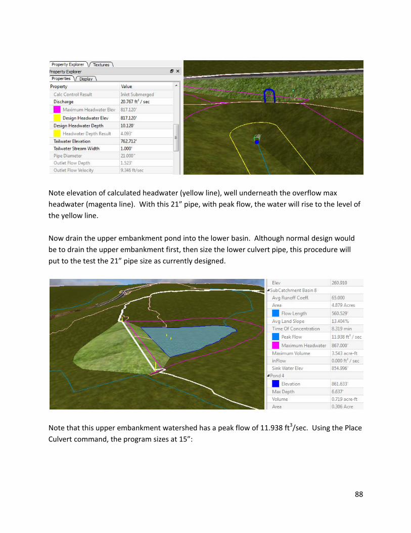
Note elevation of calculated headwater (yellow line), well underneath the overflow max headwater (magenta line). With this 21” pipe, with peak flow, the water will rise to the level of the yellow line. Now drain the upper embankment pond into the lower basin. Although normal design would be to drain the upper embankment first, then size the lower culvert pipe, this procedure will put to the test the 21” pipe size as currently designed.

Note that this upper embankment watershed has a peak flow of 11.938 ft3/sec. Using the Place Culvert command, the program sizes at 15”:

88

If you recalculate the Storm Event, note the effect on the lower culvert pipe (goes to 24”) and its yellow maximum headwater line: Hw=4.93 has risen to Hw=5.968. So the additional water has an effect. Pipe outlet velocities have increased.

If the Design Method is changed to Calculate Headwater, you can change the pipe size back to 21” to see the effect:

The 21” pipe won’t work any longer—the yellow line reaches the Maximum Headwater Elevation and overflows. If you click into Storm Event 1, the current design will be tested. You can then select any designed pipe, click on PDF Report and all Storm Events that are selected will be reported on page 2 of the Standard Pipe Report.

89

Adding a Scenario for Rational: Under the File pulldown menu, you can select Add Scenario:

In the new Scenario 2, choose the US68Merge5Pond1.tin. Select Rational method. Go to Tools pulldown menu and change to the KY Rainfall events as shown here:

Users of Carlson Hydrology can find the Rainfall libraries in c:\Carlson Projects\Settings as shown above. With this library selected, many options appear within the Property Explorer. You may need to switch back to SCS and back to Rational again to get any new Rainfall Library freshly recognized. Among the Kentucky Rainfall Intensity Libraries is the Maysville option.

This library can be viewed and edited within the Carlson Hydrology module, as shown:

90

Note that you can choose different rainfall durations. Use the Universal Rational Method and a 10-year storm event. Using the Universal and Dekalb Rational Methods, the duration for Volume Calculation is a fixed multiple of the computed Tc (time of concentration), 11x for Universal and 10x for Dekalb. For Modified Rational Method, the user-entered duration is used for volume calculations. But for peak flow, the Tc itself is used to interpolate the rainfall intensity. So to test the use of interpolated rainfall intensity in inches/hour, choose the Modified Rational Method with a 10-year return period. Note that “.rn” files always store rainfall in inches/hour, and convert to metric (cm/hour) for purposes of presentation. If you have a table of rainfall in cm/hour, you would need to convert it to inches/hour if you want to edit an existing rainfall table, save it and re-use it for metric calculations. To repeat, Rational Rainfall tables are stored in inches/hour. The next step in the process is to Calculate the Storm Event. Before clicking the Calculate Storm Event icon, set the runoff coefficient to whatever applies, such as 0.65.

The Rain Intensity of 5.8 in/hour is interpolated for the 9.07 minute Tc, leading to peak flow of 18.3 ft3/sec for the upper embankment pond watershed.

91

Pipe Length “Projecting” vs Headwalls: A smaller pipe length will be calculated if a headwall is used versus using only a standard “projecting” pipe. For the pipe-only scenario, place a pipe in the low point of the pond and connect through to the toe of the slope of the embankment as shown below:

An 18” pipe is calculated with a length of 139.397’, headwater depth result of 5.2’. (Note if that headwater is considered too high, switch to Design Headwater Mode and enter a larger pipe size such as 24”.) Now delete the pipe (select it in the Scene Explorer and press Delete).

Choose the icon that draws the pipe and applies headwalls in one process: Place the pipe at the same positions and choose the NCDOT top-left headwall from the list.

92

The pipe length is now reduced to 118.2’ (over 20’) as the headwall treatment pushes into the hill. A smaller headwall could easily accommodate the pipe above. Two examples of culverts with headwalls pushing into the hill (reducing pipe length) are shown below:

Use File, Save to CAD, to bring the pipe designs, including the modified DTM surfaces, back to CAD by LandXML.

C. Visual Indicators Certain design flaws will produce visual indicators in the Graphics Window. If a pipe is draw with a positive slope from the inlet to the outlet, water will not be able to flow through it. This error is indicated by a yellow pipe as shown below. Notice that the inlet (at the right) is in the pond and the outlet is at a higher elevation.

93

If multiple pipes are being used to drain a ponding area, you may accidently cross the pipes. This error will be indicated by coloring the crossing pipes red as shown below.

Another visual indicator is a red exclamation point hovering above a pond. This is shown if the addition of a culvert causes a pond to overflow. In the below picture, the pond requires an extra ~3,000 ft3 of volume to prevent overflow. This excess volume is reported in the tool tip.

94

D. Inserting, Editing, and Designing Headwalls Once the culverts have been designed, headwalls may be added, edited, and incorporated into the surface. As mentioned in Chapter 1 Section C, headwalls can be placed using the Insert Headwall Icon. Clicking this icon will bring up the Headwall Library which lists a variety of headwall designs. To add a headwall to a pipe, simply drag-and-drop the headwall from the library to the inlet or outlet. This will place the culvert on both ends of the pipe. To change the headwall, simply drag-and-drop another headwall onto the invert of interest. It is important to note that once a headwall has been placed, dragging-and-dropping a new headwall in place will only change one of the headwalls. This allows you to use a different headwalls for the outlet and the inlet. Once a headwall has been placed, the pipe will cut through the headwall. Making changes to the pipe such as the number of barrels or pipe diameter will also be reflected by the headwall, and changing the pipe position will move the headwall along with it. As with other 3D objects, the visibility and transparency of the headwall is listed under the Display tab of the Property Explorer. Selecting a headwall will show three types of grips on the headwall itself. The red cylinder allows you move the headwall along the length of the pipe. The blue cube allows you to move the headwall and the pipe. The two yellow spheres control the rotation of the headwall about the vertical axis. These grips are shown below.

The white lines around the headwall are visual indicators of the Headwall Grading Properties shown in the Property Explorer. These properties are visually described in the below picture. These lines can be toggled on and off in the Property Explorer.

95

Once the grading parameters have been set, the surface can be edited to reflect the new grading solution using one of the two icons shown below. These icons are listed in the Property Explorer when the headwall is selected. The icon on the left will execute the ‘Auto-Design Headwall’ command while the icon on the right will execute the ‘Grade to Surface’ command.

The ‘Grade to Surface’ command creates a new grading solution based on the headwall’s current location. This will produce results as shown below.

96

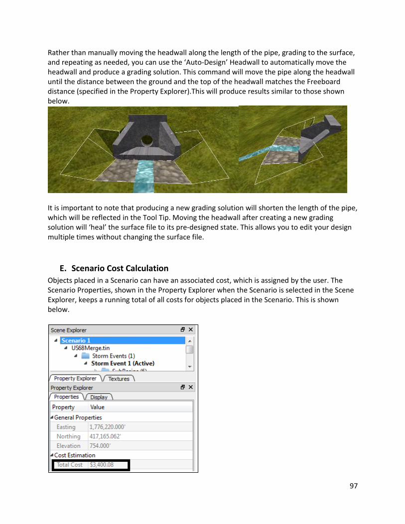
Rather than manually moving the headwall along the length of the pipe, grading to the surface, and repeating as needed, you can use the ‘Auto-Design’ Headwall to automatically move the headwall and produce a grading solution. This command will move the pipe along the headwall until the distance between the ground and the top of the headwall matches the Freeboard distance (specified in the Property Explorer).This will produce results similar to those shown below.

It is important to note that producing a new grading solution will shorten the length of the pipe, which will be reflected in the Tool Tip. Moving the headwall after creating a new grading solution will ‘heal’ the surface file to its pre-designed state. This allows you to edit your design multiple times without changing the surface file.

E. Scenario Cost Calculation Objects placed in a Scenario can have an associated cost, which is assigned by the user. The Scenario Properties, shown in the Property Explorer when the Scenario is selected in the Scene Explorer, keeps a running total of all costs for objects placed in the Scenario. This is shown below.

97

Costs can be assigned to three types of objects: culverts, headwalls, and generic/custom 3D objects. To assign a cost to specific culvert, simply select the culvert and edit the Unit Cost in the Property Explorer. The Unit Cost is the cost per ft/meter of pipe, and the default value is set to $2.00/ft. The Total Cost is simply the Unit Cost of the pipe multiplied by the total pipe length. Costs can be assigned to headwalls within the Headwall Library to affect all headwalls of that type, or the cost can be assigned to single instances of a headwall. To edit the default cost of a specific type of headwall, open the Headwall Library, select the headwall of interest, then click Edit Properties (outlined below). Here you can edit the Unit Cost of the headwall, which will be applied to every new headwall of this type. To edit the cost of a single instance of a headwall, simply use the same method as when editing the unit cost of a culvert. Costs can be applied to generic/custom 3D Objects in the same method as headwalls.

Once costs have been assigned to objects, you can inspect the total cost of a specific Scenario. This can be a useful tool for comparing the cost of materials for multiple Scenarios.

98

V. PDF Reporting and Exporting to CAD

A. PDF Reports on Culverts and Watersheds PDF reports can be generated to organize information about culverts and the watersheds with which they interact. To generate a report, you can click the Culver Pipe Report icon, shown here to the left. The below picture shows a small portion of the default PDF template that can be used for reporting.

You can also create your own PDF template using Adobe software which supports forms and form fields, such as Adobe Acrobat Pro. Customized reports can be created from scratch, or from a scanned form. The below image shows a portion of a blank, custom form to be populated with information from Precision 3D Culverts. Notice that this form calls for the return periods and tailwater depths for the culvert of interest.

This form can be populated by creating text boxes in the appropriate location on the form and inserting the corresponding Precision 3D form field. The below image shows the form partially prepared for use with Precision 3D Culverts. Once a report is generated, these form fields will be replaced with the corresponding design value/name.

99

Once the PDF template has been edited with the appropriate form fields, it can be saved and placed in the C:\ProgramData\Carlson Software\Precision3DCulverts\Data\Report Templates folder for use. Note that to access the C:\ProgramData folder, you will need to enable ‘Show Hidden Folders’ in Windows. This can be done through the Windows Control Panel > Appearance and Personalization > Folder Options > View Tab > Hidden Files and Folders > Show hidden files, folders, and drives. Once the template is placed in the appropriate folder, simply return to Precision 3D Culverts, click the Culvert Pipe Report icon, and select the template. A list of the supported form field codes is provided below.

• PipeCulvert.Name • PipeCulvert.Diameter • PipeCulvert.Length • PipeCulvert.Mannings • PipeCulvert.Shape • PipeCulvert.Material • PipeCulvert.Width • PipeCulvert.Rise • PipeCulvert.Slope • PipeCulvert.Barrels • PipeCulvert.Inlet • PipeCulvert.Inlet.Elev • PipeCulvert.Inlet.GIS • PipeCulvert.Inlet.GIS.Elev • PipeCulvert.Inlet.Easting • PipeCulvert.Inlet.Latitude • PipeCulvert.Inlet.Longitude • PipeCulvert.Inlet.Northing • PipeCulvert.Outlet.Elev • PipeCulvert.Outlet.GIS • PipeCulvert.Outlet.GIS.Elev • PipeCulvert.Outlet.Latitude • PipeCulvert.Outlet.Northing • PipeCulvert.Outlet.Longitude • PipeCulvert.Outlet.Easting • PipeCulvert.Result.1Year.Rainfall • PipeCulvert.Result.1Year.Discharge • PipeCulvert.Result.1Year.Headwater • PipeCulvert.Result.1Year.OutletVelocity • PipeCulvert.Result.1Year.Tailwater • PipeCulvert.Result.1Year.FlowDepth

• PipeCulvert.Result.5Year.Headwater • PipeCulvert.Result.5Year.OutletVelocity • PipeCulvert.Result.5Year.Tailwater • PipeCulvert.Result.5Year.FlowDepth • PipeCulvert.Result.5Year.FlowControl • PipeCulvert.Result.5Year.Rainfall • PipeCulvert.Result.10Year.Rainfall • PipeCulvert.Result.10Year.Discharge • PipeCulvert.Result.10Year.Headwater • PipeCulvert.Result.10Year.OutletVelocity • PipeCulvert.Result.10Year.Tailwater • PipeCulvert.Result.10Year.FlowDepth • PipeCulvert.Result.10Year.FlowControl • PipeCulvert.Result.25Year.Rainfall • PipeCulvert.Result.25Year.Discharge • PipeCulvert.Result.25Year.Headwater • PipeCulvert.Result.25Year.OutletVelocity • PipeCulvert.Result.25Year.Tailwater • PipeCulvert.Result.25Year.FlowDepth • PipeCulvert.Result.25Year.FlowControl • PipeCulvert.Result.50Year.Rainfall • PipeCulvert.Result.50Year.Discharge • PipeCulvert.Result.50Year.Headwater • PipeCulvert.Result.50Year.OutletVelocity • PipeCulvert.Result.50Year.Tailwater • PipeCulvert.Result.50Year.FlowDepth • PipeCulvert.Result.50Year.FlowControl • PipeCulvert.Result.100Year.Rainfall • PipeCulvert.Result.100Year.Discharge • PipeCulvert.Result.100Year.Headwater • PipeCulvert.Result.100Year.OutletVelocity

100

• PipeCulvert.Result.1Year.FlowControl • PipeCulvert.Result.2Year.Rainfall • PipeCulvert.Result.2Year.Discharge • PipeCulvert.Result.2Year.FlowControl • PipeCulvert.Result.2Year.FlowDepth • PipeCulvert.Result.2Year.Tailwater • PipeCulvert.Result.2Year.OutletVelocity • PipeCulvert.Result.2Year.Headwater • PipeCulvert.Result.5Year.Discharge

• PipeCulvert.Result.100Year.Tailwater • PipeCulvert.Result.100Year.FlowDepth • PipeCulvert.Result.100Year.FlowControl • Watershed.SubBasin.Name • Watershed.SubBasin.Area • Watershed.SubBasin.FlowCalculationMethod • Watershed.SubBasin.Coefficient • Watershed.SubBasin.FlowLength • Watershed.SubBasin.TC • Watershed.SubBasin.PeakFlow

B. Exporting Plan, Profile, Pipe Networks, and Revised DTM Data to CAD Once a scenario has been designed, you can easily export the culvert and watershed information to CAD by clicking File Pulldown Menu > Save to CAD. This action creates a LandXML file, a .dxf (drawing exchange file), and a .sew (Carlson Sewer Network file) of the culverts in the scenario. If Precision 3D Culverts was opened with the ‘P3DCULVERT’ command in CAD, this action will also automatically draw the watershed and flow information, and then prompt you to draw the updated surface (showing the new grading solution for headwalls) and pipe information. If Precision 3D Culverts was opened directly from the desktop, you will need to import the files into CAD manually. For this reason, it is recommended that you always open Precision 3D Culverts through CAD rather than opening the program directly through the desktop.

If you have opened Precision 3D Culverts through CAD, you will see the below dialog box upon exiting the program and returning to CAD. Clicking ‘Yes’ will draw the triangulation mesh or the grid file surface,

depending on the type of surface you originally loaded into the program. You will also be prompted to draw the plan view labels for the culvert. The below pictures show the three tabs available for plan view labeling. The Structure Labels tab allows you to select the labels that will be drawn in CAD. These can be edited by moving labels from the ‘Available’ column to the

101

‘Used’ column. Labels are moved between the columns by selecting the label and clicking the ‘Add’ or ‘Remove’ button between the two columns. Labels can also be edited with prefixes and suffixes by double clicking on the label.

The Pipe Labels tab allows you to select specific labels to be drawn for the pipe.

The General Settings tab allows you to control text height, decimal reporting,and the layers on which the labels will be drawn.

102

Once these options have been selected, the scenario will be drawn in CAD. An example of a culvert and watershed information as it will be drawn in CAD is given below

103

VI. 3D Object Insertion

A. Inserting 3D Objects

This icon allows you to add 3D objects to the Graphics Window, making your project appear more realistic. Precision 3D Culverts comes with a small library of objects such as Vehicles, Trees, Utilities, and more. To place an object, click this icon to open the 3D Object Library, shown below. The left column in the window shows the various object categories. The middle column shows the objects

within the category, and the right column shows a second preview and the properties associated with the selected object. Before placing an object, you can edit the properties as well as the preview image by clicking the respective buttons. To place an object, simply click the category of interest and drag-and-drop the object into the Graphics Window. The dialog window will auto-hide once the cursor is in the Graphics Window. You can also place multiple objects by double clicking the object and then selecting the insertion points in the Graphics Window.

104

Once placed, the object(s) will be listed in the Scene Explorer under the Generic Objects folder. When selected, the object properties will be shown in the Property Explorer, which you can then edit dynamically. As another means of editing the objects, you can use any of the three grips shown in the below picture. The blue grip allows you to move the object’s insertion point, the yellow grip controls the rotation of the object, and the red grip controls the height of the object.

Object Properties

• Height – controls the height of the object • Vertical Scale – applies a vertical scale to the object’s height • Perpendicular to Surface – controls whether the object is oriented in the horizontal

plane or in line with the slope at the insertion point • Model Y is Up – controls the orientation of the object; this can be especially useful

when adding your own 3D objects to the Object Library • Animation Line/Animation Speed – discussed in detail below

B. Expanding the 3D Object Library In addition to the included objects, you can add your own 3D objects to the 3D Object Library. This can be done by simply placing the objects in the proper directory on your computer. By default, 3D objects are stored in the C:\ProgramData\CarlsonSoftware\Precision3DCulverts\Data\models\Generic Models directory. Objects must be placed in a folder within one of the category folders. For example, in the below picture the ‘Cylinder.skp’ object has been placed in the “Cylinder” folder the “My 3D Objects” category folder. Precision 3D currently supports .skp and .obj formats for 3D Objects. It is

105

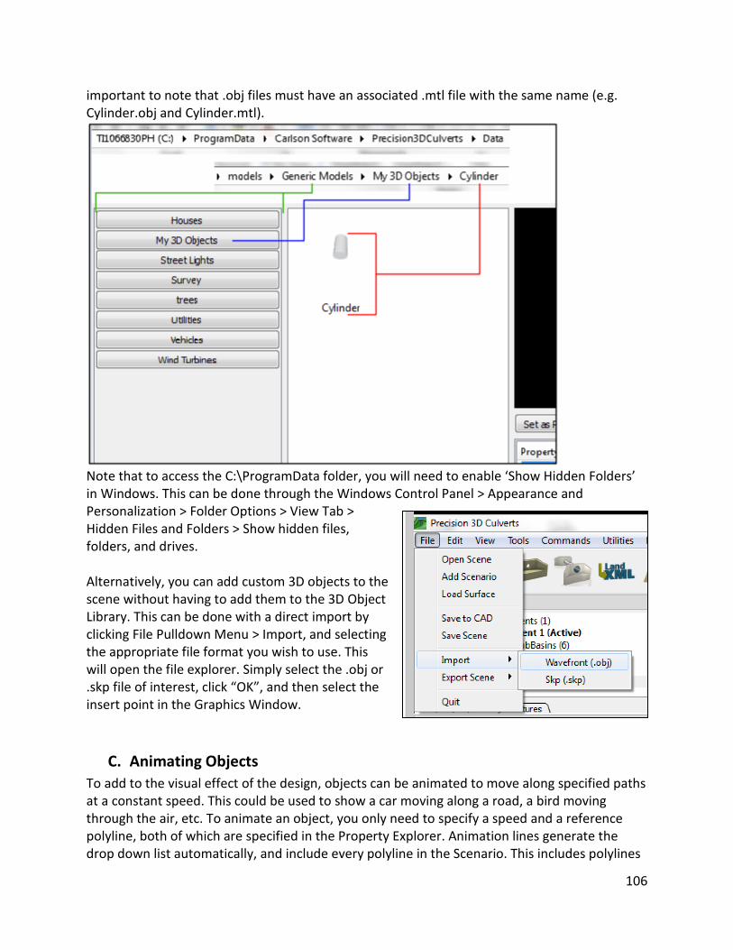
important to note that .obj files must have an associated .mtl file with the same name (e.g. Cylinder.obj and Cylinder.mtl).

Note that to access the C:\ProgramData folder, you will need to enable ‘Show Hidden Folders’ in Windows. This can be done through the Windows Control Panel > Appearance and Personalization > Folder Options > View Tab > Hidden Files and Folders > Show hidden files, folders, and drives. Alternatively, you can add custom 3D objects to the scene without having to add them to the 3D Object Library. This can be done with a direct import by clicking File Pulldown Menu > Import, and selecting the appropriate file format you wish to use. This will open the file explorer. Simply select the .obj or .skp file of interest, click “OK”, and then select the insert point in the Graphics Window.

C. Animating Objects To add to the visual effect of the design, objects can be animated to move along specified paths at a constant speed. This could be used to show a car moving along a road, a bird moving through the air, etc. To animate an object, you only need to specify a speed and a reference polyline, both of which are specified in the Property Explorer. Animation lines generate the drop down list automatically, and include every polyline in the Scenario. This includes polylines

106

that you draw yourself, which can be done using the Draw Polyline tool (see Section II Part B for detailed information). Drawn polylines will be shown at the bottom of the list. Once these parameters are specified, the objects will automatically start moving along the polyline.

107

VII. LandXML Files

A. Importing LandXML Files LandXML files can be imported using the icon shown on the left. The command can also be executed by These can be in the form of storm sewer systems, parcel boundaries, or alignments. To import a LandXML, simply click the icon and select the file. The below picture shows an example of a sewer system that has been imported to further visualize the project.

B. Exporting LandXML Surfaces, Pipe Networks, and Hydrology Data

108

Culverts and surfaces can be saved to a LandXML format once they have been designed. This can be done by clicking File Pulldown Menu > Save to CAD. Even though you may not have a CAD platform available to you, this will create a LandXML file of the culverts and the surface, as well as a .dxf which shows the 3-dimesional linework of the outer side of the pipes (this linework does not show pipe thickness). An example of pipe’s .dxf file is shown with contour lines in the below picture, and is intended primarily for visualization of the pipe.

109

VIII. System/Program Performance A. Required/Recommended Hardware

Minimum Requirements

• CPU: dual core Pentium 2.0GHz (or equivalent AMD processor) • RAM: 8GB DDR3, DDR4 1333GHz • Disk: Install requires 400MB free space • Video Card: hardware accelerated DirectX 9 or OpenGL 3.3 and above with dedicated

2GB VRAM, Nvidia GTX 400 series (or AMD/ATI equivalent) and above

Recommended • CPU: quad core Core i5 or i7 3.0GHz • RAM: 16GB DDR3, DDR4 2400Ghz • Disk: Install requires 400MB free space • Video Card: dedicated nVidia GTX700 series or above (or equivalent AMD/ATI video),

hardware accelerated drivers for DirectX 9 or OpenGL 3.3 and above with 4GB dedicated VRAM

OS: Windows 7 x64, service pack 1 or above

B. Ways to Improve Speed

Precision 3D Culverts can place a high demand on computer hardware, but it is expected that some users will need to change program settings to match the capabilities of their hardware. There are several ways to reduce hardware demand so that the program can be used on less powerful computers. Type of Surface File The type of surface file used for watershed analysis can have a great impact on computation time as well as visual representation of the scenario. Although there are three types of surface files that can be used within Precision 3D Culverts – TIN, LandXML, and Grids (binary and ASCII format) - it is highly recommended to use TIN or LandXML formats as they allow for better representation of flow lines and in general require less computation time. These two surfaces are characterized by triangles with vertices on an irregular network. Grid surfaces, however, have data points set at a regular grid spacing, which limits the accuracy of the surface by the grid resolution. The below pictures show the same surface represented as a 25’ x 25’ Grid, a 5’ x 5’ Grid, and a TIN file.

110

25’ x 25’ Grid 5’ x 5’ Grid TIN Surface As seen above, grids tend to show less detail than TIN surfaces. In order to match the general resolution of a TIN surface, the Grid spacing must be made very small, which in turn requires longer computation times. As an example from a simple time test, the above TIN surface required less than 1/10th of the time to calculate a storm event compared to that of the 5’ x 5’ Grid. Although the 25’ x 25’ Grid required less time to calculate a storm event compared to the TIN file, the lack of detail shows that this surface cannot provide an accurate representation of the flow paths or pond storage volumes. For this reason, it is highly recommended to use TIN or LandXML files for hydrology analysis as they allow for faster and more accurate computations. Further comparison of surface files is provided in the Time Test section of this chapter. Subdividing and Simplifying Surfaces Some surface files, even in TIN and LandXML format, may be too large to allow reasonable calculation times for hydrologic analysis. In these instances, it is recommended to either subdivide or simplify the surface file. This can be done easily within the Carlson Civil 2015 module. The below picture shows a TIN surface which covers a rather large area with a high level of detail. This surface could require a significant amount of time to analyze in Precision 3D Culverts. However, this surface file may cover more area than is of interest or it may provide more detail than is necessary.

111

If only a section of the surface is required for analysis, such as the outlined section in the above picture, this area can be isolated and saved as a new surface file for analysis. To isolate this section of the surface in Carlson 2015 Civil, draw a closed polyline around the area of interest, then use the Carlson 2015 Civil Module > Surface Pulldown Menu > Triangulation File Utilities command. Load the TIN file of interest, then click ‘Pick Bounding Polyline’ to select the polyline marking out the area of interest as shown below.

You can then click ‘Next’ to show the TIN editing options. To save the selected area as a new surface, simply click ‘Save as TIN’ with the Output Options set to include only the Insides and

112

the Border as shown below. The new surface will be more manageable than the full surface and will allow for faster computations.

If subdividing the surface is not an option, you can simplify the TIN file to show less detail and thus provide for faster computations. Using Triangulation File Utilities as before, simply load the surface and click ‘Next’. On the next dialog screen, click ‘Simplify’, which will bring up a new dialog box as shown below. Here you can specify a tolerance to remove detail from the surface. In the below picture, the tolerance has been set to 0.3 and to use 3 passes. This will allow the program to remove vertices from the TIN surface which will change the surface elevation by less than 0.3 feet/meters. This process will be repeated 3 times as specified by the number of passes. It is recommended to compare various levels of surface simplification to ensure accurate results.

Once a surface has been simplified, it can be saved as a new surface file for analysis within Precision 3D. Video Settings The below picture shows the Video Settings which can be edited to increase program performance. Depending on your hardware specifications, you may need to edit a combination of these settings to maximize performance. These settings can be found by clicking Tools > Settings > System Tab.

113

Precision 3D Culverts can be run on one of two Video Drivers: OpenGL and DirectX 9.0. Certain graphics cards support one or the other, but higher end graphics cards often support both. The best way to select one driver over the other is to simply try both of them and using the one that provides better results (speed, level of detail, lighting, etc.). It is important to note that some features, specifically the thickness of the polyline, cannot be edited when using the DirectX 9.0 driver. The Refresh Rate determines the number of times the Graphics Window will be updated in a second. The higher the refresh rate, the more fluid the animations and camera movements. This value can be turned down from the default value of 30 Hz to improve program performance. It should be noted, however, that decreasing this value will produce choppier camera movements, which could be incorrectly interpreted as the program running slowly. The Z Far setting controls how much of the scene is shown to the user. This essentially allows you to view features within the specified units from the viewing position. For example, the above pictures shows a Z Distance of 10,000. This will allow you to see all surface features up to a distance of 10,000 ft/m. The ‘Show Water Reflections’ option is one of the most demanding video settings within Precision 3D. This option is purely for visual effect, and can be turned off if it causes the program to run slowly. The below picture shows the difference between showing and hiding the water reflections. The effect of this feature on calculation time can be found in the Time Test section of this chapter.

114

Shadows can be toggled on and off for added visualization of the scene. Although this option places less of a demand on hardware than the ‘Show Water Reflections’ option, it can still slow down the program. Turning off this option will increase program performance, but it is recommended to first edit the Render Resolution, the Shadow Map Resolution, and the Shadow Filter Type, as shadows allow you to see changes in slope across the surface. The Render Resolution determines the amount of detail shown on surfaces and objects. A higher resolution will result in a higher quality picture, but this could slow down your machine. The Shadow Map Resolution determines the smoothness of the shadows. The below pictures show a shaded surface with a shadow map resolution of 1024 and 4096, respectively. Using the default resolution of 1024 is generally sufficient for shadow visualization.

The Shadow Filter Type – The Shadow filter type controls the ‘smoothness of the shadow, measured in Percentage-Closer Filtering (PCF). In simple terms, the higher the PCF value, the smoother the shadow. The below pictures show an object with a PCF setting of 4 and 16, respectively. Notice how the second picture has a less jagged shadow.

115

The other settings listed in the Video Options dialog box have a negligible effect on performance, and for this reason are not detailed here. Running Multiple Programs As previously mentioned, an absolute minimum of 8 GB of RAM is required for Precision 3D Culverts, but 16 GB of RAM is encouraged. If you find that Precision 3D is running slowly, you may need to try closing other programs first. To put this in perspective, the below picture shows the Windows Task Manager with a few programs running. Notice that programs such as AutoCAD can use over 2.2 GB of RAM. By closing other programs before opening Precision 3D, you will free up more of the computer’s memory and thus allow for faster computations and higher-end visualization effects.

116

C. Time Tests

The following time tests are meant to serve as an example of how Precision 3D performs on various machines at various video settings. All tests were performed on machines that were recently reset – the only installed programs aside from defaults were Precision 3D and the Carlson Civil Suite on AutoCAD. Precision 3D build 31581 (released 3/25/2015) was the only program running during the time tests. Specifications for the three test machines are given below.

The time tests were performed to isolate the effect of single variables on overall performance. This is meant to give the user an idea of how a combination of the video settings might affect performance on their own machine. For tests where a variable was not changed, the settings shown below were applied. Unless otherwise specified, the US68Merge.tin surface file was used for analysis (this surface file is included with the installation of Precision 3D).

Test 1 – Render Resolution The results of Test 1 show the effects of larger render resolution sizes for the three test machines. This test was performed using the US68Merge.tin surface file.

117

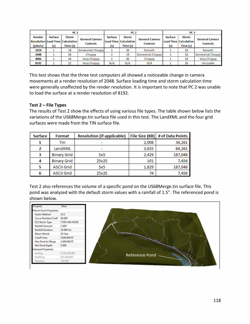
This test shows that the three test computers all showed a noticeable change in camera movements at a render resolution of 2048. Surface loading time and storm calculation time were generally unaffected by the render resolution. It is important to note that PC 2 was unable to load the surface at a render resolution of 8192. Test 2 – File Types The results of Test 2 show the effects of using various file types. The table shown below lists the variations of the US68Merge.tin surface file used in this test. The LandXML and the four grid surfaces were made from the TIN surface file.

Test 2 also references the volume of a specific pond on the US68Merge.tin surface file. This pond was analyzed with the default storm values with a rainfall of 1.5”. The referenced pond is shown below.

118

The results of Test 2 are given below.

*Cannot complete computation Test 2 shows that for a given surface, the time required to load the surface can vary significantly depending on the file format and resolution. Although the time required to load the surface is not greatly affected by the file format, the storm calculation time can be greatly affected. Notice how the 5x5 grids contain a very large number of points relative to the TIN file, which results in a longer calculation time. It should also be noted that such a small grid cell is required to attain the level of detail of a TIN file, which was demonstrated in an earlier section of this chapter. It can also be seen that the pond reference volumes can vary by as much as 10% compared to the volume suggested by the TIN file. In conclusion, the results of this test show that TIN files allow for relatively short computation times while maintaining a high level of surface detail. Test 3 – Show Water Reflections The results of Test 3 show the effect of the Show Water Reflections option. This test made use of the US68Merge.tin surface file.

All three test machines show that Water Reflections place a very high demand on computer hardware. This feature requires the use of high-end graphics capabilities and processing speeds. Although this feature has very little effect on storm calculation times, it greatly decreases the fluidity of the camera controls due to the hardware limitations of the test machines.

119