Precision of FLEET Velocimetry using High-Speed … of FLEET Velocimetry using High-Speed CMOS Camera Systems ... LaVision Imager scientific CMOS (sCMOS) and a Photron FASTCAM SA-X2,

American Institute of Aeronautics and Astronautics

1

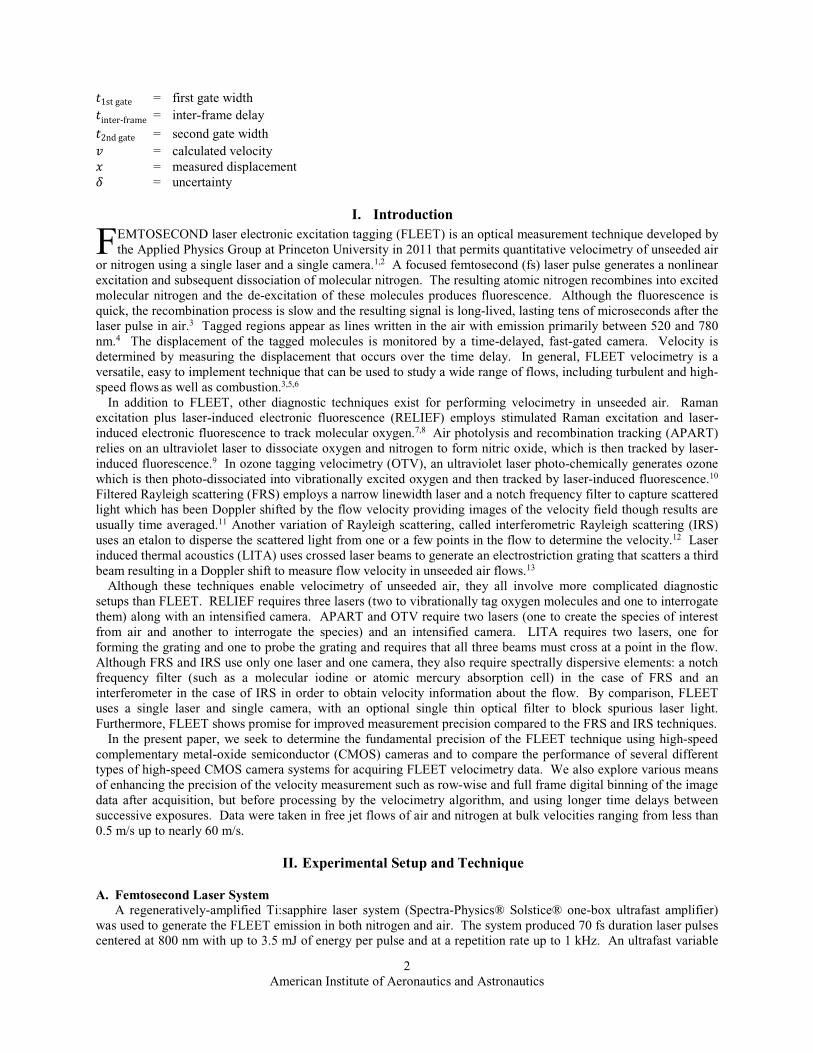
Precision of FLEET Velocimetry using High-Speed CMOS Camera Systems

Christopher J. Peters1 Princeton University, Princeton, New Jersey, 08544

Paul M. Danehy2 and Brett F. Bathel3 NASA Langley Research Center, Hampton, Virginia, 23681

Naibo Jiang 4 Spectral Energies, LLC, Dayton, Ohio, 45431

Nathan D. Calvert5 and Richard B. Miles6

Princeton University, Princeton, New Jersey, 08544

Femtosecond laser electronic excitation tagging (FLEET) is an optical measurement technique that permits quantitative velocimetry of unseeded air or nitrogen using a single laser and a single camera. In this paper, we seek to determine the fundamental precision of the FLEET technique using high-speed complementary metal-oxide semiconductor (CMOS) cameras. Also, we compare the performance of several different high-speed CMOS camera systems for acquiring FLEET velocimetry data in air and nitrogen free-jet flows. The precision was defined as the standard deviation of a set of several hundred single-shot velocity measurements. Methods of enhancing the precision of the measurement were explored such as digital binning (similar in concept to on-sensor binning, but done in post-processing), row-wise digital binning of the signal in adjacent pixels and increasing the time delay between successive exposures. These techniques generally improved precision; however, binning provided the greatest improvement to the un-intensified camera systems which had low signal-to-noise ratio. When binning row-wise by 8 pixels (about the thickness of the tagged region) and using an inter-frame delay of 65 µs, precisions of 0.5 m/s in air and 0.2 m/s in nitrogen were achieved. The camera comparison included a pco.dimax HD, a LaVision Imager scientific CMOS (sCMOS) and a Photron FASTCAM SA-X2, along with a two-stage LaVision HighSpeed IRO intensifier. Excluding the LaVision Imager sCMOS, the cameras were tested with and without intensification and with both short and long inter-frame delays. Use of intensification and longer inter-frame delay generally improved precision. Overall, the Photron FASTCAM SA-X2 exhibited the best performance in terms of greatest precision and highest signal-to-noise ratio primarily because it had the largest pixels.

Nomenclature = number of binned pixels = root mean square signal noise = signal intensity = time delay

1 Graduate Student, Mechanical and Aerospace Engineering, D225 E-Quad, Olden Street, AIAA Student Member. 2 Research Scientist, Advanced Measurements and Data Systems Branch, Mail Stop 493, AIAA Associate Fellow. 3 Research Scientist, Advanced Measurements and Data Systems Branch, Mail Stop 493, AIAA Senior Member. 4 Research Scientist, Spectral Energies, LLC, 5100 Springfield Street, Suite 301, AIAA Senior Member. 5 Graduate Student, Mechanical and Aerospace Engineering, D225 E-Quad, Olden Street, AIAA Student Member. 6 Professor Emeritus, Mechanical and Aerospace Engineering, D225 E-Quad, Olden Street, AIAA Fellow.

https://ntrs.nasa.gov/search.jsp?R=20160006055 2018-05-26T23:45:42+00:00Z


2

1stgate = first gate width inter-frame = inter-frame delay 2ndgate = second gate width = calculated velocity = measured displacement = uncertainty

I. Introduction EMTOSECOND laser electronic excitation tagging (FLEET) is an optical measurement technique developed by the Applied Physics Group at Princeton University in 2011 that permits quantitative velocimetry of unseeded air

or nitrogen using a single laser and a single camera.1,2 A focused femtosecond (fs) laser pulse generates a nonlinear excitation and subsequent dissociation of molecular nitrogen. The resulting atomic nitrogen recombines into excited molecular nitrogen and the de-excitation of these molecules produces fluorescence. Although the fluorescence is quick, the recombination process is slow and the resulting signal is long-lived, lasting tens of microseconds after the laser pulse in air.3 Tagged regions appear as lines written in the air with emission primarily between 520 and 780 nm.4 The displacement of the tagged molecules is monitored by a time-delayed, fast-gated camera. Velocity is determined by measuring the displacement that occurs over the time delay. In general, FLEET velocimetry is a versatile, easy to implement technique that can be used to study a wide range of flows, including turbulent and high-speed flows as well as combustion.3,5,6

In addition to FLEET, other diagnostic techniques exist for performing velocimetry in unseeded air. Raman excitation plus laser-induced electronic fluorescence (RELIEF) employs stimulated Raman excitation and laser-induced electronic fluorescence to track molecular oxygen.7,8 Air photolysis and recombination tracking (APART) relies on an ultraviolet laser to dissociate oxygen and nitrogen to form nitric oxide, which is then tracked by laser-induced fluorescence.9 In ozone tagging velocimetry (OTV), an ultraviolet laser photo-chemically generates ozone which is then photo-dissociated into vibrationally excited oxygen and then tracked by laser-induced fluorescence.10 Filtered Rayleigh scattering (FRS) employs a narrow linewidth laser and a notch frequency filter to capture scattered light which has been Doppler shifted by the flow velocity providing images of the velocity field though results are usually time averaged.11 Another variation of Rayleigh scattering, called interferometric Rayleigh scattering (IRS) uses an etalon to disperse the scattered light from one or a few points in the flow to determine the velocity.12 Laser induced thermal acoustics (LITA) uses crossed laser beams to generate an electrostriction grating that scatters a third beam resulting in a Doppler shift to measure flow velocity in unseeded air flows.13

Although these techniques enable velocimetry of unseeded air, they all involve more complicated diagnostic setups than FLEET. RELIEF requires three lasers (two to vibrationally tag oxygen molecules and one to interrogate them) along with an intensified camera. APART and OTV require two lasers (one to create the species of interest from air and another to interrogate the species) and an intensified camera. LITA requires two lasers, one for forming the grating and one to probe the grating and requires that all three beams must cross at a point in the flow. Although FRS and IRS use only one laser and one camera, they also require spectrally dispersive elements: a notch frequency filter (such as a molecular iodine or atomic mercury absorption cell) in the case of FRS and an interferometer in the case of IRS in order to obtain velocity information about the flow. By comparison, FLEET uses a single laser and single camera, with an optional single thin optical filter to block spurious laser light. Furthermore, FLEET shows promise for improved measurement precision compared to the FRS and IRS techniques.

In the present paper, we seek to determine the fundamental precision of the FLEET technique using high-speed complementary metal-oxide semiconductor (CMOS) cameras and to compare the performance of several different types of high-speed CMOS camera systems for acquiring FLEET velocimetry data. We also explore various means of enhancing the precision of the velocity measurement such as row-wise and full frame digital binning of the image data after acquisition, but before processing by the velocimetry algorithm, and using longer time delays between successive exposures. Data were taken in free jet flows of air and nitrogen at bulk velocities ranging from less than 0.5 m/s up to nearly 60 m/s.

II. Experimental Setup and Technique

A. Femtosecond Laser System A regeneratively-amplified Ti:sapphire laser system (Spectra-Physics® Solstice® one-box ultrafast amplifier)

was used to generate the FLEET emission in both nitrogen and air. The system produced 70 fs duration laser pulses centered at 800 nm with up to 3.5 mJ of energy per pulse and at a repetition rate up to 1 kHz. An ultrafast variable

F


3

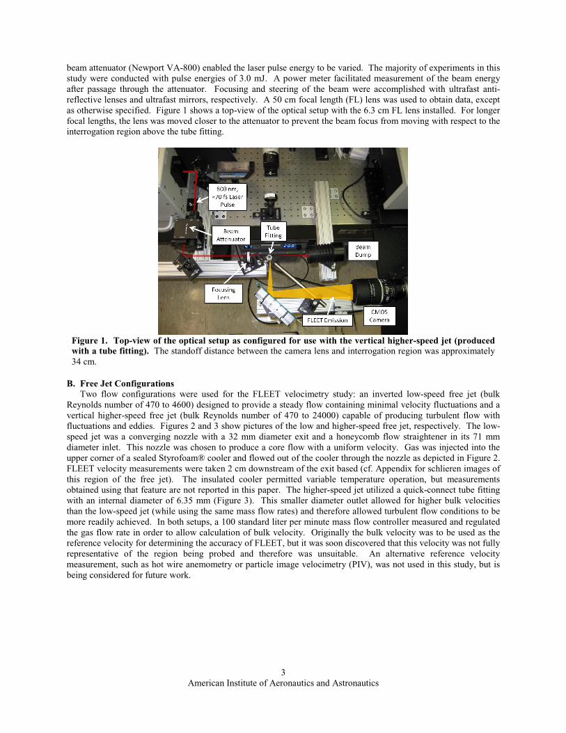
beam attenuator (Newport VA-800) enabled the laser pulse energy to be varied. The majority of experiments in this study were conducted with pulse energies of 3.0 mJ. A power meter facilitated measurement of the beam energy after passage through the attenuator. Focusing and steering of the beam were accomplished with ultrafast anti-reflective lenses and ultrafast mirrors, respectively. A 50 cm focal length (FL) lens was used to obtain data, except as otherwise specified. Figure 1 shows a top-view of the optical setup with the 6.3 cm FL lens installed. For longer focal lengths, the lens was moved closer to the attenuator to prevent the beam focus from moving with respect to the interrogation region above the tube fitting.

Figure 1. Top-view of the optical setup as configured for use with the vertical higher-speed jet (produced with a tube fitting). The standoff distance between the camera lens and interrogation region was approximately 34 cm.

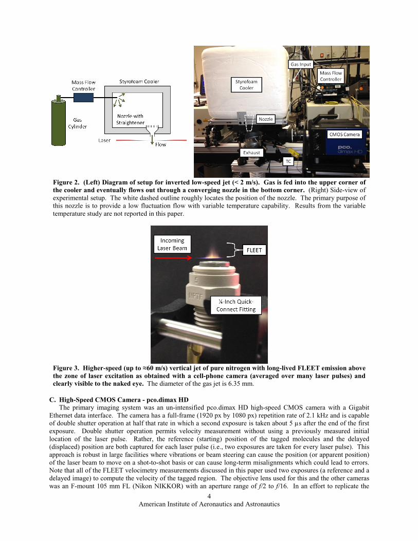
B. Free Jet Configurations Two flow configurations were used for the FLEET velocimetry study: an inverted low-speed free jet (bulk

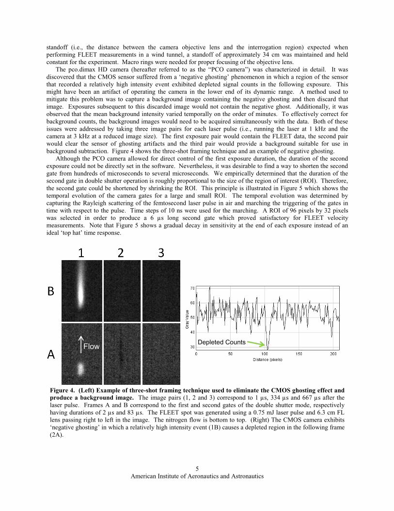
Reynolds number of 470 to 4600) designed to provide a steady flow containing minimal velocity fluctuations and a vertical higher-speed free jet (bulk Reynolds number of 470 to 24000) capable of producing turbulent flow with fluctuations and eddies. Figures 2 and 3 show pictures of the low and higher-speed free jet, respectively. The low-speed jet was a converging nozzle with a 32 mm diameter exit and a honeycomb flow straightener in its 71 mm diameter inlet. This nozzle was chosen to produce a core flow with a uniform velocity. Gas was injected into the upper corner of a sealed Styrofoam® cooler and flowed out of the cooler through the nozzle as depicted in Figure 2. FLEET velocity measurements were taken 2 cm downstream of the exit based (cf. Appendix for schlieren images of this region of the free jet). The insulated cooler permitted variable temperature operation, but measurements obtained using that feature are not reported in this paper. The higher-speed jet utilized a quick-connect tube fitting with an internal diameter of 6.35 mm (Figure 3). This smaller diameter outlet allowed for higher bulk velocities than the low-speed jet (while using the same mass flow rates) and therefore allowed turbulent flow conditions to be more readily achieved. In both setups, a 100 standard liter per minute mass flow controller measured and regulated the gas flow rate in order to allow calculation of bulk velocity. Originally the bulk velocity was to be used as the reference velocity for determining the accuracy of FLEET, but it was soon discovered that this velocity was not fully representative of the region being probed and therefore was unsuitable. An alternative reference velocity measurement, such as hot wire anemometry or particle image velocimetry (PIV), was not used in this study, but is being considered for future work.


4

Figure 2. (Left) Diagram of setup for inverted low-speed jet (< 2 m/s). Gas is fed into the upper corner of the cooler and eventually flows out through a converging nozzle in the bottom corner. (Right) Side-view of experimental setup. The white dashed outline roughly locates the position of the nozzle. The primary purpose of this nozzle is to provide a low fluctuation flow with variable temperature capability. Results from the variable temperature study are not reported in this paper.

Figure 3. Higher-speed (up to ≈60 m/s) vertical jet of pure nitrogen with long-lived FLEET emission above the zone of laser excitation as obtained with a cell-phone camera (averaged over many laser pulses) and clearly visible to the naked eye. The diameter of the gas jet is 6.35 mm.

C. High-Speed CMOS Camera - pco.dimax HD The primary imaging system was an un-intensified pco.dimax HD high-speed CMOS camera with a Gigabit

Ethernet data interface. The camera has a full-frame (1920 px by 1080 px) repetition rate of 2.1 kHz and is capable of double shutter operation at half that rate in which a second exposure is taken about 5 µs after the end of the first exposure. Double shutter operation permits velocity measurement without using a previously measured initial location of the laser pulse. Rather, the reference (starting) position of the tagged molecules and the delayed (displaced) position are both captured for each laser pulse (i.e., two exposures are taken for every laser pulse). This approach is robust in large facilities where vibrations or beam steering can cause the position (or apparent position) of the laser beam to move on a shot-to-shot basis or can cause long-term misalignments which could lead to errors. Note that all of the FLEET velocimetry measurements discussed in this paper used two exposures (a reference and a delayed image) to compute the velocity of the tagged region. The objective lens used for this and the other cameras was an F-mount 105 mm FL (Nikon NIKKOR) with an aperture range of f/2 to f/16. In an effort to replicate the


5

standoff (i.e., the distance between the camera objective lens and the interrogation region) expected when performing FLEET measurements in a wind tunnel, a standoff of approximately 34 cm was maintained and held constant for the experiment. Macro rings were needed for proper focusing of the objective lens.

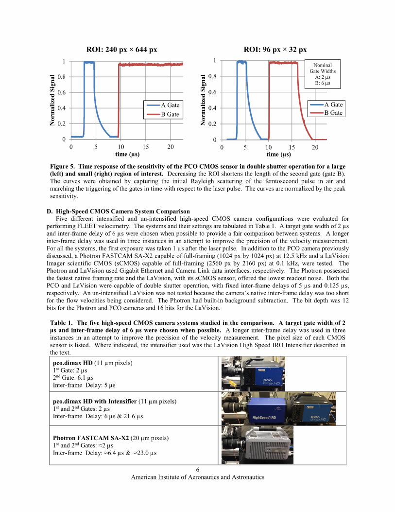
The pco.dimax HD camera (hereafter referred to as the “PCO camera”) was characterized in detail. It was discovered that the CMOS sensor suffered from a ‘negative ghosting’ phenomenon in which a region of the sensor that recorded a relatively high intensity event exhibited depleted signal counts in the following exposure. This might have been an artifact of operating the camera in the lower end of its dynamic range. A method used to mitigate this problem was to capture a background image containing the negative ghosting and then discard that image. Exposures subsequent to this discarded image would not contain the negative ghost. Additionally, it was observed that the mean background intensity varied temporally on the order of minutes. To effectively correct for background counts, the background images would need to be acquired simultaneously with the data. Both of these issues were addressed by taking three image pairs for each laser pulse (i.e., running the laser at 1 kHz and the camera at 3 kHz at a reduced image size). The first exposure pair would contain the FLEET data, the second pair would clear the sensor of ghosting artifacts and the third pair would provide a background suitable for use in background subtraction. Figure 4 shows the three-shot framing technique and an example of negative ghosting.

Although the PCO camera allowed for direct control of the first exposure duration, the duration of the second exposure could not be directly set in the software. Nevertheless, it was desirable to find a way to shorten the second gate from hundreds of microseconds to several microseconds. We empirically determined that the duration of the second gate in double shutter operation is roughly proportional to the size of the region of interest (ROI). Therefore, the second gate could be shortened by shrinking the ROI. This principle is illustrated in Figure 5 which shows the temporal evolution of the camera gates for a large and small ROI. The temporal evolution was determined by capturing the Rayleigh scattering of the femtosecond laser pulse in air and marching the triggering of the gates in time with respect to the pulse. Time steps of 10 ns were used for the marching. A ROI of 96 pixels by 32 pixels was selected in order to produce a 6 µs long second gate which proved satisfactory for FLEET velocity measurements. Note that Figure 5 shows a gradual decay in sensitivity at the end of each exposure instead of an ideal ‘top hat’ time response.

Figure 4. (Left) Example of three-shot framing technique used to eliminate the CMOS ghosting effect and produce a background image. The image pairs (1, 2 and 3) correspond to 1 µs, 334 µs and 667 µs after the laser pulse. Frames A and B correspond to the first and second gates of the double shutter mode, respectively having durations of 2 µs and 83 µs. The FLEET spot was generated using a 0.75 mJ laser pulse and 6.3 cm FL lens passing right to left in the image. The nitrogen flow is bottom to top. (Right) The CMOS camera exhibits ‘negative ghosting’ in which a relatively high intensity event (1B) causes a depleted region in the following frame (2A).

FlowDepleted Counts


6

0

0.2

0.4

0.6

0.8

1

0 5 10 15 20

Nor

mal

ized

Sig

nal

time (µs)

ROI: 240 px × 644 px

A Gate

B Gate

0

0.2

0.4

0.6

0.8

1

0 5 10 15 20

Nor

mal

ized

Sig

nal

time (µs)

ROI: 96 px × 32 px

A GateB Gate

NominalGate Widths

A: 2 µsB: 6 µs

Figure 5. Time response of the sensitivity of the PCO CMOS sensor in double shutter operation for a large (left) and small (right) region of interest. Decreasing the ROI shortens the length of the second gate (gate B). The curves were obtained by capturing the initial Rayleigh scattering of the femtosecond pulse in air and marching the triggering of the gates in time with respect to the laser pulse. The curves are normalized by the peak sensitivity.

D. High-Speed CMOS Camera System Comparison Five different intensified and un-intensified high-speed CMOS camera configurations were evaluated for

performing FLEET velocimetry. The systems and their settings are tabulated in Table 1. A target gate width of 2 µs and inter-frame delay of 6 µs were chosen when possible to provide a fair comparison between systems. A longer inter-frame delay was used in three instances in an attempt to improve the precision of the velocity measurement. For all the systems, the first exposure was taken 1 µs after the laser pulse. In addition to the PCO camera previously discussed, a Photron FASTCAM SA-X2 capable of full-framing (1024 px by 1024 px) at 12.5 kHz and a LaVision Imager scientific CMOS (sCMOS) capable of full-framing (2560 px by 2160 px) at 0.1 kHz, were tested. The Photron and LaVision used Gigabit Ethernet and Camera Link data interfaces, respectively. The Photron possessed the fastest native framing rate and the LaVision, with its sCMOS sensor, offered the lowest readout noise. Both the PCO and LaVision were capable of double shutter operation, with fixed inter-frame delays of 5 µs and 0.125 µs, respectively. An un-intensified LaVision was not tested because the camera’s native inter-frame delay was too short for the flow velocities being considered. The Photron had built-in background subtraction. The bit depth was 12 bits for the Photron and PCO cameras and 16 bits for the LaVision.

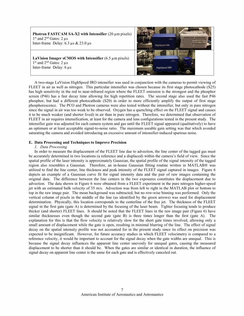
Table 1. The five high-speed CMOS camera systems studied in the comparison. A target gate width of 2 µs and inter-frame delay of 6 µs were chosen when possible. A longer inter-frame delay was used in three instances in an attempt to improve the precision of the velocity measurement. The pixel size of each CMOS sensor is listed. Where indicated, the intensifier used was the LaVision High Speed IRO Intensifier described in the text.

pco.dimax HD (11 µm pixels) 1st Gate: 2 µs 2nd Gate: 6.1 µs Inter-frame Delay: 5 µs

pco.dimax HD with Intensifier (11 µm pixels) 1st and 2nd Gates: 2 µs Inter-frame Delay: 6 µs & 21.6 µs

Photron FASTCAM SA-X2 (20 µm pixels) 1st and 2nd Gates: ≈2 µs Inter-frame Delay: ≈6.4 µs & ≈23.0 µs


7

Photron FASTCAM SA-X2 with Intensifier (20 µm pixels) 1st and 2nd Gates: 2 µs Inter-frame Delay: 6.3 µs & 23.0 µs

LaVision Imager sCMOS with Intensifier (6.5 µm pixels) 1st and 2nd Gates: 2 µs Inter-frame Delay: 6 µs

A two-stage LaVision HighSpeed IRO intensifier was used in conjunction with the cameras to permit viewing of

FLEET in air as well as nitrogen. This particular intensifier was chosen because its first stage photocathode (S25) has high sensitivity in the red to near-infrared region where the FLEET emission is the strongest and the phosphor screen (P46) has a fast decay time allowing for high repetition rates. The second stage also used the fast P46 phosphor, but had a different photocathode (S20) in order to more efficiently amplify the output of first stage phosphorescence. The PCO and Photron cameras were also tested without the intensifier, but only in pure nitrogen since the signal in air was too weak to be observed. Oxygen has a quenching effect on the FLEET signal and causes it to be much weaker (and shorter lived) in air than in pure nitrogen. Therefore, we determined that observation of FLEET in air requires intensification, at least for the camera and lens configurations tested in the present study. The intensifier gain was adjusted for each camera system and gas until the FLEET signal appeared (qualitatively) to have an optimum or at least acceptable signal-to-noise ratio. The maximum useable gain setting was that which avoided saturating the camera and avoided introducing an excessive amount of intensifier-induced spurious noise.

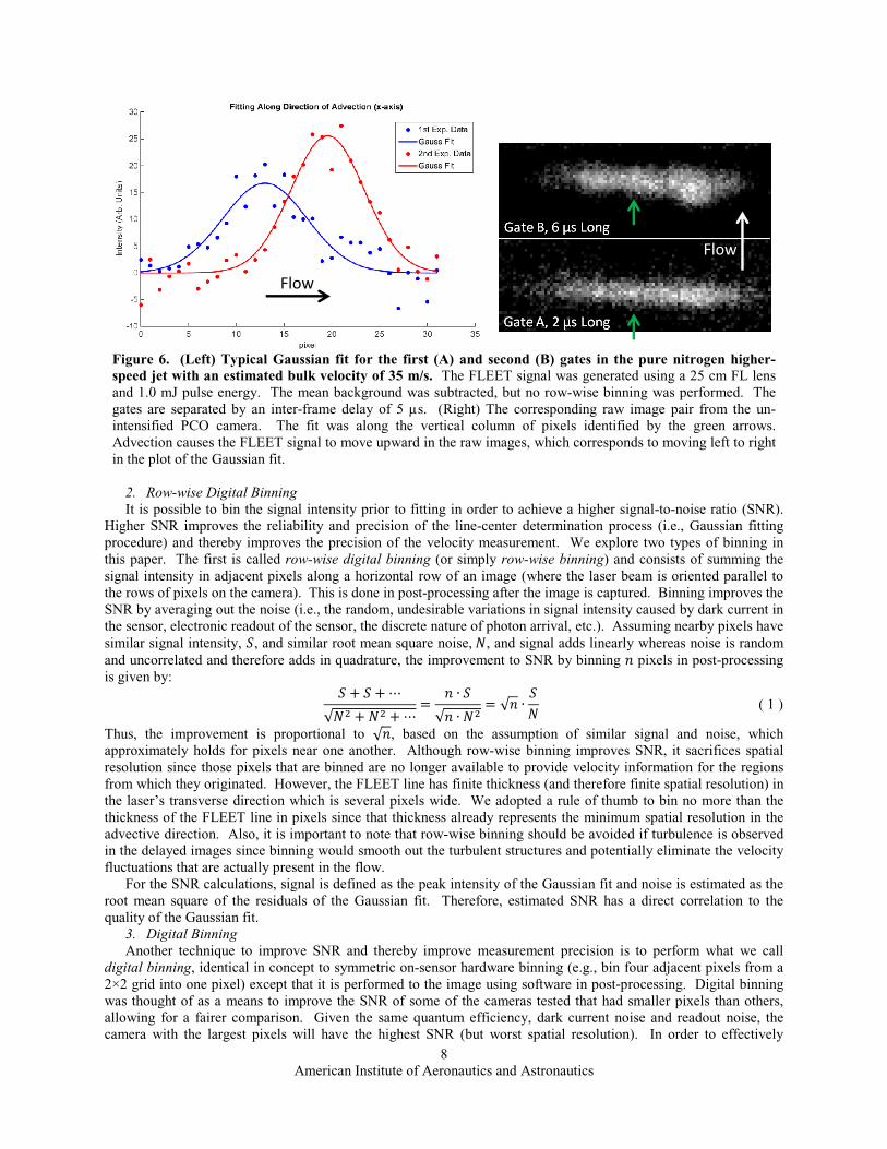
E. Data Processing and Techniques to Improve Precision 1. Data Processing In order to measure the displacement of the FLEET line due to advection, the line center of the tagged gas must

be accurately determined in two locations (a reference and a displaced) within the camera’s field of view. Since the spatial profile of the laser intensity is approximately Gaussian, the spatial profile of the signal intensity of the tagged region also resembles a Gaussian. Therefore, an in-house Gaussian fitting routine written in MATLAB® was utilized to find the line center, line thickness and peak intensity of the FLEET signal captured in images. Figure 6 depicts an example of a Gaussian curve fit for signal intensity data and the pair of raw images containing the original data. The difference between the line centers in the two exposures constitutes the displacement due to advection. The data shown in Figure 6 were obtained from a FLEET experiment in the pure nitrogen higher-speed jet with an estimated bulk velocity of 35 m/s. Advection was from left to right in the MATLAB plot or bottom to top in the raw image pair. The mean background was subtracted, but no row-wise binning was performed. Only the vertical column of pixels in the middle of the line (as identified by the green arrows) was used for displacement determination. Physically, this location corresponds to the centerline of the free jet. The thickness of the FLEET signal in the first gate (gate A) is determined by the focusing of the laser beam. Tighter focusing tends to produce thicker (and shorter) FLEET lines. It should be noted that the FLEET lines in the raw image pair (Figure 6) have similar thicknesses even though the second gate (gate B) is three times longer than the first (gate A). The explanation for this is that the flow velocity is relatively slow for the short gate times involved, allowing only a small amount of displacement while the gate is open, resulting in minimal blurring of the line. The effect of signal decay on the spatial intensity profile was not accounted for in the present study since its effect on precision was expected to be insignificant. However, for future accuracy studies in which FLEET velocimetry is compared to a reference velocity, it would be important to account for the signal decay when the gate widths are unequal. This is because the signal decay influences the apparent line center unevenly for unequal gates, causing the measured displacement to be shorter than it should be. When the gates are similar or identical in duration, the influence of signal decay on apparent line center is the same for each gate and is effectively canceled out.


8

Figure 6. (Left) Typical Gaussian fit for the first (A) and second (B) gates in the pure nitrogen higher-speed jet with an estimated bulk velocity of 35 m/s. The FLEET signal was generated using a 25 cm FL lens and 1.0 mJ pulse energy. The mean background was subtracted, but no row-wise binning was performed. The gates are separated by an inter-frame delay of 5 µs. (Right) The corresponding raw image pair from the un-intensified PCO camera. The fit was along the vertical column of pixels identified by the green arrows. Advection causes the FLEET signal to move upward in the raw images, which corresponds to moving left to right in the plot of the Gaussian fit.

2. Row-wise Digital Binning It is possible to bin the signal intensity prior to fitting in order to achieve a higher signal-to-noise ratio (SNR).

Higher SNR improves the reliability and precision of the line-center determination process (i.e., Gaussian fitting procedure) and thereby improves the precision of the velocity measurement. We explore two types of binning in this paper. The first is called row-wise digital binning (or simply row-wise binning) and consists of summing the signal intensity in adjacent pixels along a horizontal row of an image (where the laser beam is oriented parallel to the rows of pixels on the camera). This is done in post-processing after the image is captured. Binning improves the SNR by averaging out the noise (i.e., the random, undesirable variations in signal intensity caused by dark current in the sensor, electronic readout of the sensor, the discrete nature of photon arrival, etc.). Assuming nearby pixels have similar signal intensity, , and similar root mean square noise, , and signal adds linearly whereas noise is random and uncorrelated and therefore adds in quadrature, the improvement to SNR by binning pixels in post-processing is given by: ⋯√ ⋯ ∙√ ∙ √ ∙ ( 1 )

Thus, the improvement is proportional to √ , based on the assumption of similar signal and noise, which approximately holds for pixels near one another. Although row-wise binning improves SNR, it sacrifices spatial resolution since those pixels that are binned are no longer available to provide velocity information for the regions from which they originated. However, the FLEET line has finite thickness (and therefore finite spatial resolution) in the laser’s transverse direction which is several pixels wide. We adopted a rule of thumb to bin no more than the thickness of the FLEET line in pixels since that thickness already represents the minimum spatial resolution in the advective direction. Also, it is important to note that row-wise binning should be avoided if turbulence is observed in the delayed images since binning would smooth out the turbulent structures and potentially eliminate the velocity fluctuations that are actually present in the flow.

For the SNR calculations, signal is defined as the peak intensity of the Gaussian fit and noise is estimated as the root mean square of the residuals of the Gaussian fit. Therefore, estimated SNR has a direct correlation to the quality of the Gaussian fit.

3. Digital Binning Another technique to improve SNR and thereby improve measurement precision is to perform what we call

digital binning, identical in concept to symmetric on-sensor hardware binning (e.g., bin four adjacent pixels from a 2×2 grid into one pixel) except that it is performed to the image using software in post-processing. Digital binning was thought of as a means to improve the SNR of some of the cameras tested that had smaller pixels than others, allowing for a fairer comparison. Given the same quantum efficiency, dark current noise and readout noise, the camera with the largest pixels will have the highest SNR (but worst spatial resolution). In order to effectively

Flow

Flow


9

increase the pixel size of the other cameras, 2×2 and 3×3 digital binning was performed on images taken by cameras with pixels respectively one-half and one-third the size of the largest pixels. Improvement to SNR occurs in the same manner as with row-wise binning (by averaging out noise) and the tradeoff is the same in that the spatial resolution is sacrificed. Digital binning offers the possibility of enhancing the SNR of cameras with smaller pixels while still maintaining the capability of the camera to revert back to higher spatial resolution, assuming the SNR penalty is acceptable.

4. Inter-frame Delay The intensified PCO and Photron cameras were tested with both short and long inter-frame delays (cf. Table 1).

The reason for this was to investigate the potential improvement to precision achieved by increasing the time delay. The time delay is computed as

inter-frame 12 ∙ 1stgate 12 ∙ 2ndgate ( 2 )

where , inter-frame, 1stgate and 2ndgate represent the time delay, inter-frame delay, first gate width and second gate width, respectively. According to basic uncertainty analysis,14 the uncertainty in a calculated velocity is ∙ ∙ ( 3 )

where and are measured displacement and calculated velocity, respectively, and the prefix denotes uncertainty in a quantity. The uncertainty in line-center determination is the primary source of random uncertainty in the measured displacement. There is also systematic uncertainty resulting from errors in magnification (i.e., the conversion from pixels to physical length). An example of temporal uncertainty is the timing jitter between the start of the gates of the image pair which causes random uncertainty in the duration of the inter-frame delay. (Note that since images are acquired well after the laser pulse, the timing jitter between the laser and camera system cancels out when using image pairs.) Since calculated velocity is given by

( 4 )

the uncertainty in velocity is given by ∙ ( 5 )

which shows that increasing the time delay acts to decrease the uncertainty in velocity — it reduces errors associated with both spatial uncertainty and temporal uncertainty. However, it should be noted that for very long time delays, finite fluorescence lifetime and diffusion of the tagged molecules reduces the SNR enough to make locating the line center difficult (i.e., imprecise). This is especially true for images taken without intensification. Thus, there is a maximum time delay that optimizes precision. A further limitation of long delay times is that the spatial resolution is proportionally worse as the gas travels a further distance. Even worse, for long delays, the idea of computing a velocity comes into question since the gas may accelerate or decelerate along this path. Moreover, long time delays would be inappropriate for flows where the turbulence timescale is shorter than the chosen time delay. Accordingly, the optimal time delay depends on the flow regime (which dictates how quickly the FLEET line will break up), the pressure and temperature of the flow (which affects the rate of diffusion of the FLEET line as well as the lifetime) and whether the flow is composed of air or nitrogen (since signal lifetimes are dramatically shorter in air than in nitrogen).

III. Results and Discussion

A. Improvement in Precision due to Row-wise Binning and Inter-frame Delay 1. No Row-wise Binning The precision was defined as the standard deviation of the set of hundreds of single-shot velocity measurements

for a particular flow rate. FLEET velocimetry was performed in the pure nitrogen higher-speed jet for a range of velocities. Figures 7 and 8 show precision results for the un-intensified and intensified Photron camera, respectively. The relevant laser and camera parameters are detailed in the figure titles and captions. The first gate was 1 µs after the laser pulse. The standard deviation contains contributions from both the imprecision of the technique (in particular, the line-center determination) and the actual velocity fluctuations of the flow. For the case of no row-wise binning (i.e., binning row-wise by one pixel), the standard deviation is similar for the low speeds and then increases as the flow speed increases. This increase occurs because the velocity fluctuations being measured are real fluctuations attributable to turbulence. The similarity in standard deviation at the lower bulk velocities (below 6 m/s) suggests that the precision is limited by the measurement technique as opposed to turbulent


10

fluctuations. Above 11 m/s, the standard deviation increases substantially, suggesting that the precision is now limited by the turbulent fluctuations of the flow.

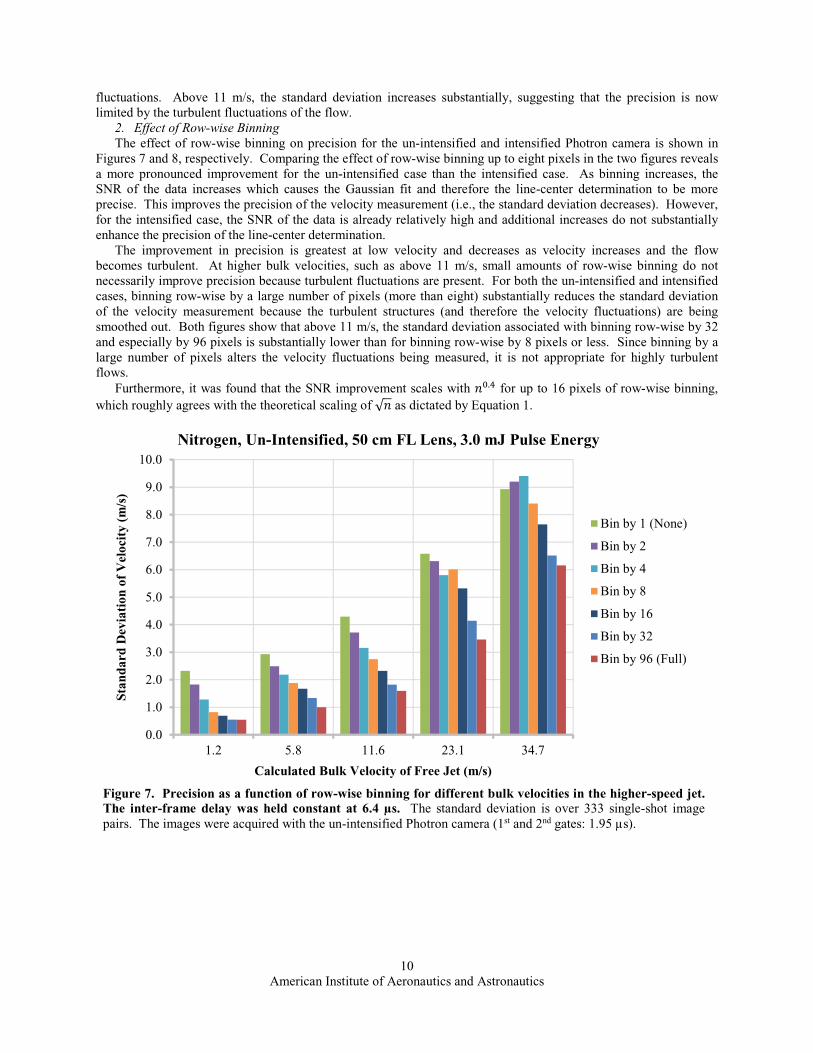
2. Effect of Row-wise Binning The effect of row-wise binning on precision for the un-intensified and intensified Photron camera is shown in

Figures 7 and 8, respectively. Comparing the effect of row-wise binning up to eight pixels in the two figures reveals a more pronounced improvement for the un-intensified case than the intensified case. As binning increases, the SNR of the data increases which causes the Gaussian fit and therefore the line-center determination to be more precise. This improves the precision of the velocity measurement (i.e., the standard deviation decreases). However, for the intensified case, the SNR of the data is already relatively high and additional increases do not substantially enhance the precision of the line-center determination.

The improvement in precision is greatest at low velocity and decreases as velocity increases and the flow becomes turbulent. At higher bulk velocities, such as above 11 m/s, small amounts of row-wise binning do not necessarily improve precision because turbulent fluctuations are present. For both the un-intensified and intensified cases, binning row-wise by a large number of pixels (more than eight) substantially reduces the standard deviation of the velocity measurement because the turbulent structures (and therefore the velocity fluctuations) are being smoothed out. Both figures show that above 11 m/s, the standard deviation associated with binning row-wise by 32 and especially by 96 pixels is substantially lower than for binning row-wise by 8 pixels or less. Since binning by a large number of pixels alters the velocity fluctuations being measured, it is not appropriate for highly turbulent flows.

Furthermore, it was found that the SNR improvement scales with . for up to 16 pixels of row-wise binning, which roughly agrees with the theoretical scaling of √ as dictated by Equation 1.

Figure 7. Precision as a function of row-wise binning for different bulk velocities in the higher-speed jet. The inter-frame delay was held constant at 6.4 µs. The standard deviation is over 333 single-shot image pairs. The images were acquired with the un-intensified Photron camera (1st and 2nd gates: 1.95 µs).

0.0

1.0

2.0

3.0

4.0

5.0

6.0

7.0

8.0

9.0

10.0

1.2 5.8 11.6 23.1 34.7

Stan

dard

Dev

iati

on o

f V

eloc

ity

(m/s

)

Calculated Bulk Velocity of Free Jet (m/s)

Nitrogen, Un-Intensified, 50 cm FL Lens, 3.0 mJ Pulse Energy

Bin by 1 (None)

Bin by 2

Bin by 4

Bin by 8

Bin by 16

Bin by 32

Bin by 96 (Full)


11

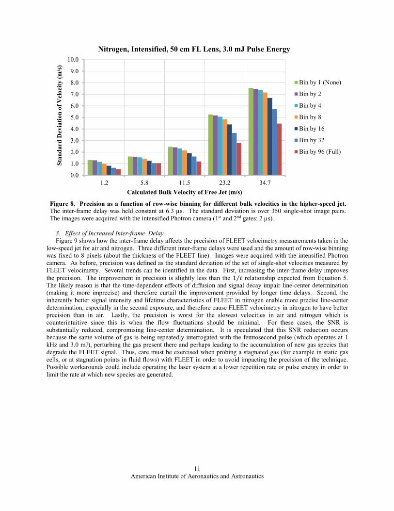
Figure 8. Precision as a function of row-wise binning for different bulk velocities in the higher-speed jet. The inter-frame delay was held constant at 6.3 µs. The standard deviation is over 350 single-shot image pairs. The images were acquired with the intensified Photron camera (1st and 2nd gates: 2 µs).

3. Effect of Increased Inter-frame Delay Figure 9 shows how the inter-frame delay affects the precision of FLEET velocimetry measurements taken in the

low-speed jet for air and nitrogen. Three different inter-frame delays were used and the amount of row-wise binning was fixed to 8 pixels (about the thickness of the FLEET line). Images were acquired with the intensified Photron camera. As before, precision was defined as the standard deviation of the set of single-shot velocities measured by FLEET velocimetry. Several trends can be identified in the data. First, increasing the inter-frame delay improves the precision. The improvement in precision is slightly less than the 1⁄ relationship expected from Equation 5. The likely reason is that the time-dependent effects of diffusion and signal decay impair line-center determination (making it more imprecise) and therefore curtail the improvement provided by longer time delays. Second, the inherently better signal intensity and lifetime characteristics of FLEET in nitrogen enable more precise line-center determination, especially in the second exposure, and therefore cause FLEET velocimetry in nitrogen to have better precision than in air. Lastly, the precision is worst for the slowest velocities in air and nitrogen which is counterintuitive since this is when the flow fluctuations should be minimal. For these cases, the SNR is substantially reduced, compromising line-center determination. It is speculated that this SNR reduction occurs because the same volume of gas is being repeatedly interrogated with the femtosecond pulse (which operates at 1 kHz and 3.0 mJ), perturbing the gas present there and perhaps leading to the accumulation of new gas species that degrade the FLEET signal. Thus, care must be exercised when probing a stagnated gas (for example in static gas cells, or at stagnation points in fluid flows) with FLEET in order to avoid impacting the precision of the technique. Possible workarounds could include operating the laser system at a lower repetition rate or pulse energy in order to limit the rate at which new species are generated.

0.0

1.0

2.0

3.0

4.0

5.0

6.0

7.0

8.0

9.0

10.0

1.2 5.8 11.5 23.2 34.7

Stan

dard

Dev

iati

on o

f V

eloc

ity

(m/s

)


Nitrogen, Intensified, 50 cm FL Lens, 3.0 mJ Pulse Energy

Bin by 1 (None)

Bin by 2

Bin by 4

Bin by 8

Bin by 16

Bin by 32

Bin by 96 (Full)


12

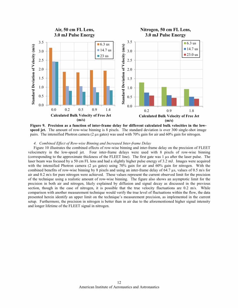
Figure 9. Precision as a function of inter-frame delay for different calculated bulk velocities in the low-speed jet. The amount of row-wise binning is 8 pixels. The standard deviation is over 300 single-shot image pairs. The intensified Photron camera (2 µs gates) was used with 70% gain for air and 60% gain for nitrogen.

4. Combined Effect of Row-wise Binning and Increased Inter-frame Delay Figure 10 illustrates the combined effects of row-wise binning and inter-frame delay on the precision of FLEET

velocimetry in the low-speed jet. Four inter-frame delays were used with 8 pixels of row-wise binning (corresponding to the approximate thickness of the FLEET line). The first gate was 1 µs after the laser pulse. The laser beam was focused by a 50 cm FL lens and had a slightly higher pulse energy of 3.2 mJ. Images were acquired with the intensified Photron camera (2 µs gates) using 70% gain for air and 60% gain for nitrogen. With the combined benefits of row-wise binning by 8 pixels and using an inter-frame delay of 64.7 µs, values of 0.5 m/s for air and 0.2 m/s for pure nitrogen were achieved. These values represent the current observed limit for the precision of the technique using a realistic amount of row-wise binning. The figure also shows an asymptotic limit for the precision in both air and nitrogen, likely explained by diffusion and signal decay as discussed in the previous section, though in the case of nitrogen, it is possible that the true velocity fluctuations are 0.2 m/s. While comparison with another measurement technique would verify the true level of fluctuations within the flow, the data presented herein identify an upper limit on the technique’s measurement precision, as implemented in the current setup. Furthermore, the precision in nitrogen is better than in air due to the aforementioned higher signal intensity and longer lifetime of the FLEET signal in nitrogen.

0.0

0.5

1.0

1.5

2.0

2.5

3.0

3.5

0.0 0.2 0.5 0.9 1.4

Stan

dard

Dev

iati

on o

f V

eloc

ity

(m/s

)


Air, 50 cm FL Lens,3.0 mJ Pulse Energy

6.3 us

14.7 us

23 us

0.0

0.5

1.0

1.5

2.0

2.5

3.0

3.5

0.2 0.9 1.8

Stan

dard

Dev

iati

on o

f V

eloc

ity

(m/s

)


Nitrogen, 50 cm FL Lens,3.0 mJ Pulse Energy

6.3 us

14.7 us

23.0 us


13

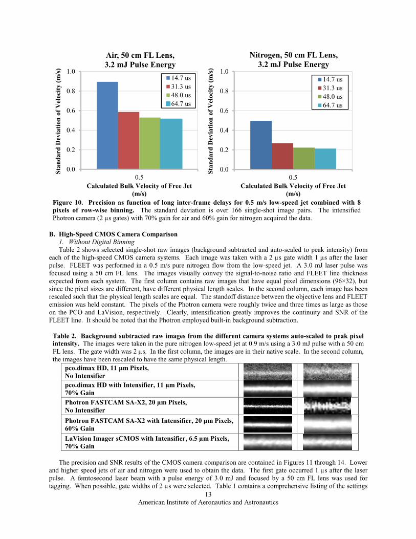
Figure 10. Precision as function of long inter-frame delays for 0.5 m/s low-speed jet combined with 8 pixels of row-wise binning. The standard deviation is over 166 single-shot image pairs. The intensified Photron camera (2 µs gates) with 70% gain for air and 60% gain for nitrogen acquired the data.

B. High-Speed CMOS Camera Comparison 1. Without Digital Binning Table 2 shows selected single-shot raw images (background subtracted and auto-scaled to peak intensity) from

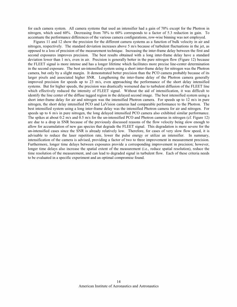
each of the high-speed CMOS camera systems. Each image was taken with a 2 µs gate width 1 µs after the laser pulse. FLEET was performed in a 0.5 m/s pure nitrogen flow from the low-speed jet. A 3.0 mJ laser pulse was focused using a 50 cm FL lens. The images visually convey the signal-to-noise ratio and FLEET line thickness expected from each system. The first column contains raw images that have equal pixel dimensions (96×32), but since the pixel sizes are different, have different physical length scales. In the second column, each image has been rescaled such that the physical length scales are equal. The standoff distance between the objective lens and FLEET emission was held constant. The pixels of the Photron camera were roughly twice and three times as large as those on the PCO and LaVision, respectively. Clearly, intensification greatly improves the continuity and SNR of the FLEET line. It should be noted that the Photron employed built-in background subtraction.

Table 2. Background subtracted raw images from the different camera systems auto-scaled to peak pixel intensity. The images were taken in the pure nitrogen low-speed jet at 0.9 m/s using a 3.0 mJ pulse with a 50 cm FL lens. The gate width was 2 µs. In the first column, the images are in their native scale. In the second column, the images have been rescaled to have the same physical length.

pco.dimax HD, 11 µm Pixels, No Intensifier pco.dimax HD with Intensifier, 11 µm Pixels, 70% Gain Photron FASTCAM SA-X2, 20 µm Pixels, No Intensifier Photron FASTCAM SA-X2 with Intensifier, 20 µm Pixels, 60% Gain LaVision Imager sCMOS with Intensifier, 6.5 µm Pixels, 70% Gain

The precision and SNR results of the CMOS camera comparison are contained in Figures 11 through 14. Lower

and higher speed jets of air and nitrogen were used to obtain the data. The first gate occurred 1 µs after the laser pulse. A femtosecond laser beam with a pulse energy of 3.0 mJ and focused by a 50 cm FL lens was used for tagging. When possible, gate widths of 2 µs were selected. Table 1 contains a comprehensive listing of the settings

0.0

0.2

0.4

0.6

0.8

1.0

0.5

Stan

dard

Dev

iati

on o

f V

eloc

ity

(m/s

)


Air, 50 cm FL Lens, 3.2 mJ Pulse Energy

14.7 us31.3 us48.0 us64.7 us

0.0

0.2

0.4

0.6

0.8

1.0

0.5

Stan

dard

Dev

iati

on o

f V

eloc

ity

(m/s

)


Nitrogen, 50 cm FL Lens, 3.2 mJ Pulse Energy

14.7 us31.3 us48.0 us64.7 us


14

for each camera system. All camera systems that used an intensifier had a gain of 70% except for the Photron in nitrogen, which used 60%. Decreasing from 70% to 60% corresponds to a factor of 5.3 reduction in gain. To accentuate the performance differences of the various camera configurations, row-wise binning was not employed.

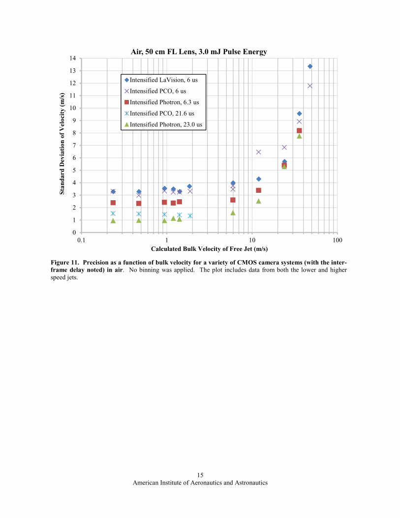
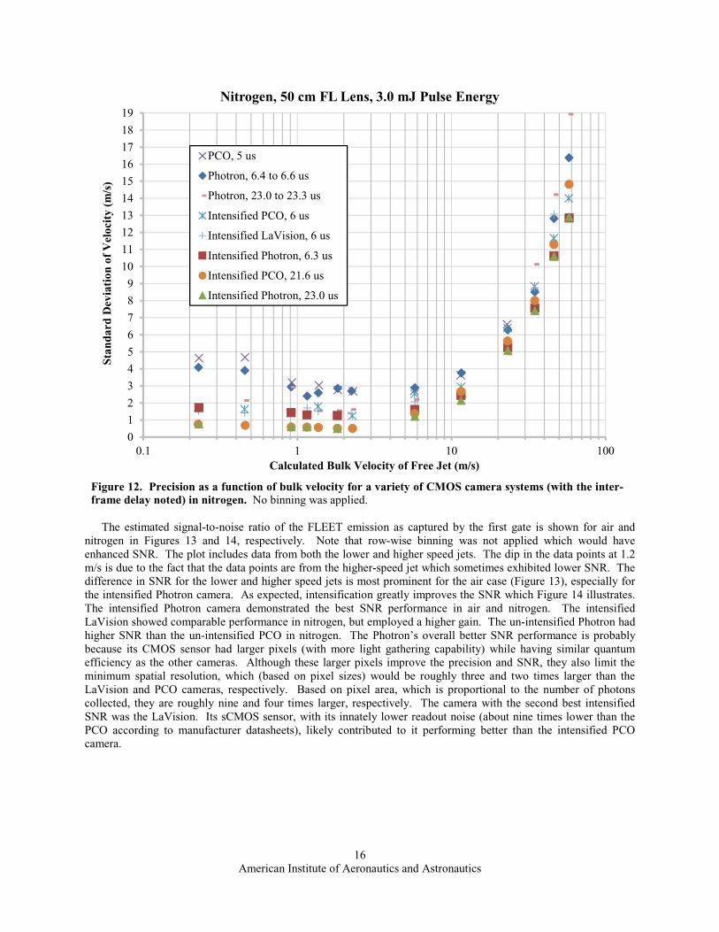
Figures 11 and 12 show the precision for the different camera systems as a function of bulk velocity in air and nitrogen, respectively. The standard deviation increases above 5 m/s because of turbulent fluctuations in the jet, as opposed to a loss of precision of the measurement technique. Increasing the inter-frame delay between the first and second exposures improves precision. The best results obtained with a long inter-frame delay have a standard deviation lower than 1 m/s, even in air. Precision is generally better in the pure nitrogen flow (Figure 12) because the FLEET signal is more intense and has a longer lifetime which facilitates more precise line-center determination in the second exposure. The best un-intensified system using a short inter-frame delay for nitrogen was the Photron camera, but only by a slight margin. It demonstrated better precision than the PCO camera probably because of its larger pixels and associated higher SNR. Lengthening the inter-frame delay of the Photron camera generally improved precision for speeds up to 23 m/s, even approaching the performance of the short delay intensified systems. But for higher speeds, the precision was drastically worsened due to turbulent diffusion of the FLEET line which effectively reduced the intensity of FLEET signal. Without the aid of intensification, it was difficult to identify the line center of the diffuse tagged region in the delayed second image. The best intensified system using a short inter-frame delay for air and nitrogen was the intensified Photron camera. For speeds up to 12 m/s in pure nitrogen, the short delay intensified PCO and LaVision cameras had comparable performance to the Photron. The best intensified system using a long inter-frame delay was the intensified Photron camera for air and nitrogen. For speeds up to 6 m/s in pure nitrogen, the long delayed intensified PCO camera also exhibited similar performance. The spikes at about 0.2 m/s and 0.5 m/s for the un-intensified PCO and Photron cameras in nitrogen (cf. Figure 12) are due to a drop in SNR because of the previously discussed reasons of the flow velocity being slow enough to allow for accumulation of new gas species that degrade the FLEET signal. This degradation is more severe for the un-intensified cases since the SNR is already relatively low. Therefore, for cases of very slow flow speed, it is advisable to reduce the laser repetition rate, lower the pulse energy or utilize an intensifier. In summary, intensification of the camera is advised, providing a factor of two to three improvement in measurement precision. Furthermore, longer time delays between exposures provide a corresponding improvement in precision; however, longer time delays also increase the spatial extent of the measurement (i.e., reduce spatial resolution), reduce the time resolution of the measurement, and can lead to degraded signal in turbulent flow. Each of these criteria needs to be evaluated in a specific experiment and an optimal compromise found.


15

Figure 11. Precision as a function of bulk velocity for a variety of CMOS camera systems (with the inter-frame delay noted) in air. No binning was applied. The plot includes data from both the lower and higher speed jets.

0

1

2

3

4

5

6

7

8

9

10

11

12

13

14

0.1 1 10 100

Stan

dard

Dev

iati

on o

f V

eloc

ity

(m/s

)


Air, 50 cm FL Lens, 3.0 mJ Pulse Energy

Intensified LaVision, 6 us

Intensified PCO, 6 us

Intensified Photron, 6.3 us

Intensified PCO, 21.6 us



16

Figure 12. Precision as a function of bulk velocity for a variety of CMOS camera systems (with the inter-frame delay noted) in nitrogen. No binning was applied.

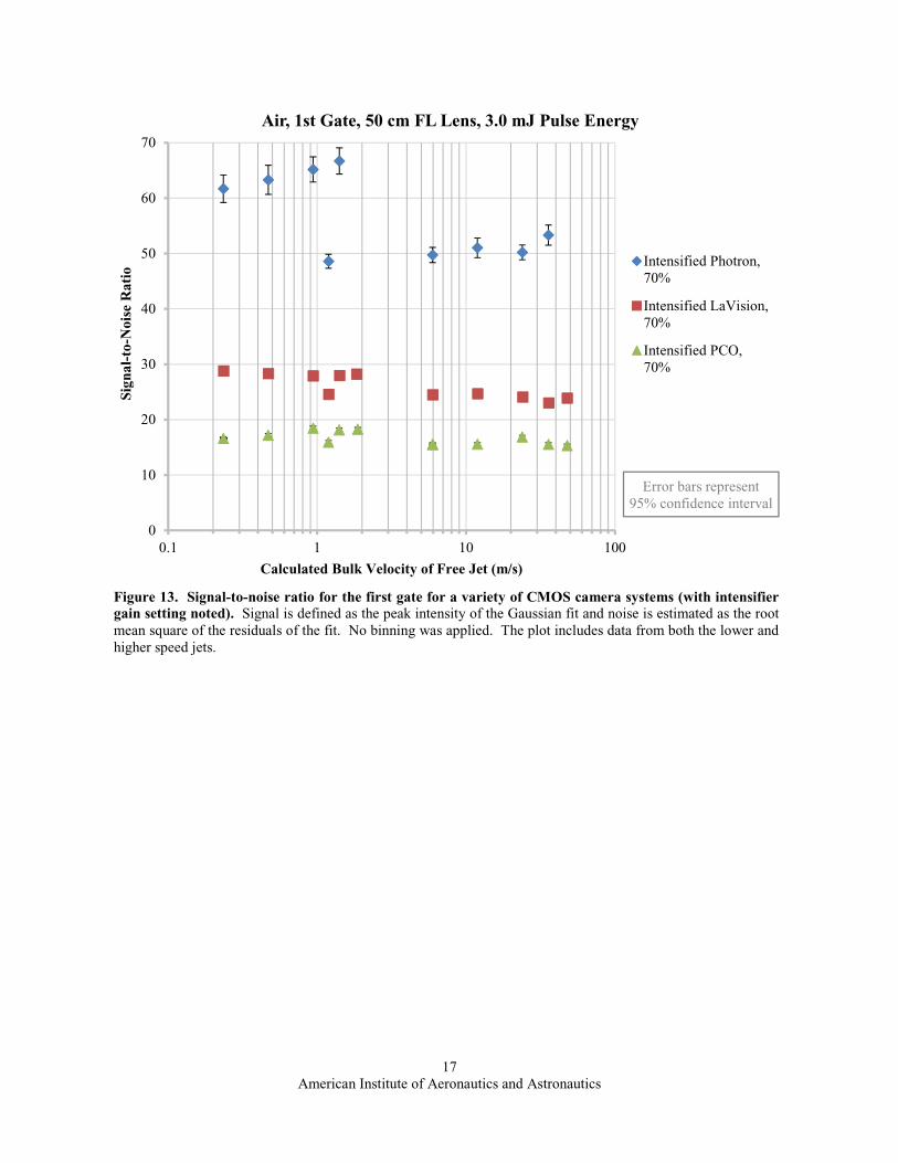
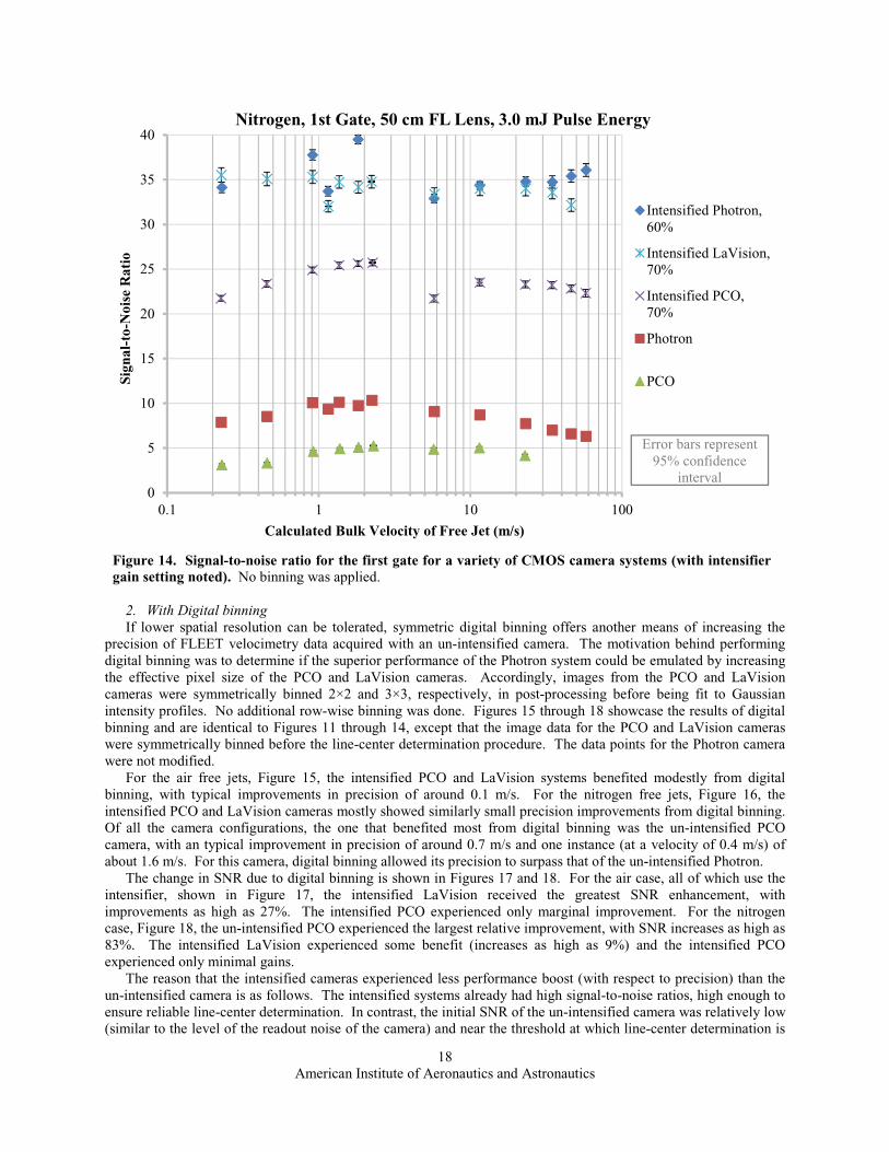
The estimated signal-to-noise ratio of the FLEET emission as captured by the first gate is shown for air and nitrogen in Figures 13 and 14, respectively. Note that row-wise binning was not applied which would have enhanced SNR. The plot includes data from both the lower and higher speed jets. The dip in the data points at 1.2 m/s is due to the fact that the data points are from the higher-speed jet which sometimes exhibited lower SNR. The difference in SNR for the lower and higher speed jets is most prominent for the air case (Figure 13), especially for the intensified Photron camera. As expected, intensification greatly improves the SNR which Figure 14 illustrates. The intensified Photron camera demonstrated the best SNR performance in air and nitrogen. The intensified LaVision showed comparable performance in nitrogen, but employed a higher gain. The un-intensified Photron had higher SNR than the un-intensified PCO in nitrogen. The Photron’s overall better SNR performance is probably because its CMOS sensor had larger pixels (with more light gathering capability) while having similar quantum efficiency as the other cameras. Although these larger pixels improve the precision and SNR, they also limit the minimum spatial resolution, which (based on pixel sizes) would be roughly three and two times larger than the LaVision and PCO cameras, respectively. Based on pixel area, which is proportional to the number of photons collected, they are roughly nine and four times larger, respectively. The camera with the second best intensified SNR was the LaVision. Its sCMOS sensor, with its innately lower readout noise (about nine times lower than the PCO according to manufacturer datasheets), likely contributed to it performing better than the intensified PCO camera.

0

1

2

3

4

5

6

7

8

9

10

11

12

13

14

15

16

17

18

19

0.1 1 10 100

Stan

dard

Dev

iati

on o

f V

eloc

ity

(m/s

)


Nitrogen, 50 cm FL Lens, 3.0 mJ Pulse Energy

PCO, 5 us

Photron, 6.4 to 6.6 us








17

Figure 13. Signal-to-noise ratio for the first gate for a variety of CMOS camera systems (with intensifier gain setting noted). Signal is defined as the peak intensity of the Gaussian fit and noise is estimated as the root mean square of the residuals of the fit. No binning was applied. The plot includes data from both the lower and higher speed jets.

0

10

20

30

40

50

60

70

0.1 1 10 100

Sign

al-t

o-N

oise

Rat

io


Air, 1st Gate, 50 cm FL Lens, 3.0 mJ Pulse Energy

Intensified Photron,70%

Intensified LaVision,70%

Intensified PCO,70%

Error bars represent 95% confidence interval


18

Figure 14. Signal-to-noise ratio for the first gate for a variety of CMOS camera systems (with intensifier gain setting noted). No binning was applied.

2. With Digital binning If lower spatial resolution can be tolerated, symmetric digital binning offers another means of increasing the

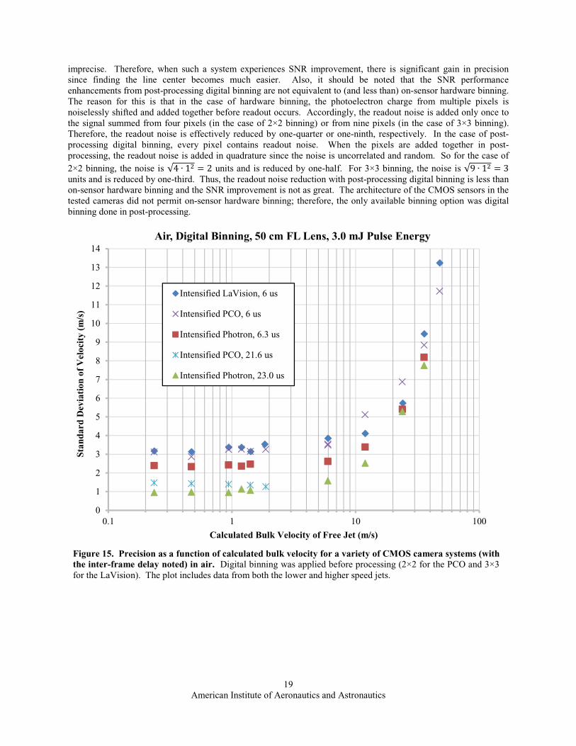
precision of FLEET velocimetry data acquired with an un-intensified camera. The motivation behind performing digital binning was to determine if the superior performance of the Photron system could be emulated by increasing the effective pixel size of the PCO and LaVision cameras. Accordingly, images from the PCO and LaVision cameras were symmetrically binned 2×2 and 3×3, respectively, in post-processing before being fit to Gaussian intensity profiles. No additional row-wise binning was done. Figures 15 through 18 showcase the results of digital binning and are identical to Figures 11 through 14, except that the image data for the PCO and LaVision cameras were symmetrically binned before the line-center determination procedure. The data points for the Photron camera were not modified.

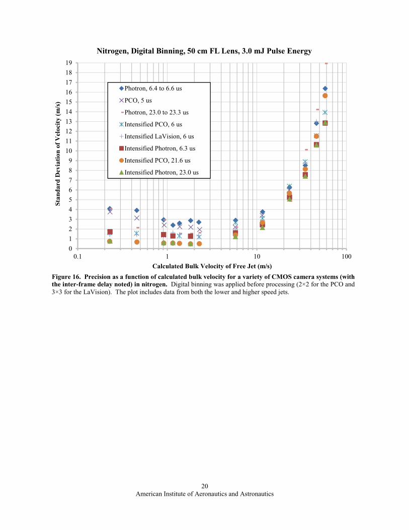
For the air free jets, Figure 15, the intensified PCO and LaVision systems benefited modestly from digital binning, with typical improvements in precision of around 0.1 m/s. For the nitrogen free jets, Figure 16, the intensified PCO and LaVision cameras mostly showed similarly small precision improvements from digital binning. Of all the camera configurations, the one that benefited most from digital binning was the un-intensified PCO camera, with an typical improvement in precision of around 0.7 m/s and one instance (at a velocity of 0.4 m/s) of about 1.6 m/s. For this camera, digital binning allowed its precision to surpass that of the un-intensified Photron.

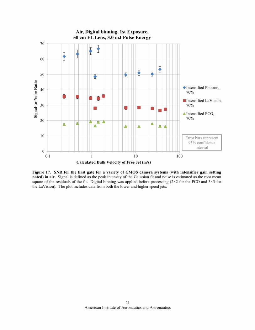
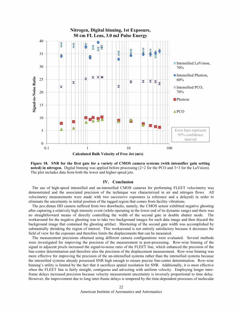
The change in SNR due to digital binning is shown in Figures 17 and 18. For the air case, all of which use the intensifier, shown in Figure 17, the intensified LaVision received the greatest SNR enhancement, with improvements as high as 27%. The intensified PCO experienced only marginal improvement. For the nitrogen case, Figure 18, the un-intensified PCO experienced the largest relative improvement, with SNR increases as high as 83%. The intensified LaVision experienced some benefit (increases as high as 9%) and the intensified PCO experienced only minimal gains.

The reason that the intensified cameras experienced less performance boost (with respect to precision) than the un-intensified camera is as follows. The intensified systems already had high signal-to-noise ratios, high enough to ensure reliable line-center determination. In contrast, the initial SNR of the un-intensified camera was relatively low (similar to the level of the readout noise of the camera) and near the threshold at which line-center determination is

0

5

10

15

20

25

30

35

40

0.1 1 10 100

Sign

al-t

o-N

oise

Rat

io


Nitrogen, 1st Gate, 50 cm FL Lens, 3.0 mJ Pulse Energy



Intensified PCO,70%

Photron

PCO

Error bars represent 95% confidence

interval


19

imprecise. Therefore, when such a system experiences SNR improvement, there is significant gain in precision since finding the line center becomes much easier. Also, it should be noted that the SNR performance enhancements from post-processing digital binning are not equivalent to (and less than) on-sensor hardware binning. The reason for this is that in the case of hardware binning, the photoelectron charge from multiple pixels is noiselessly shifted and added together before readout occurs. Accordingly, the readout noise is added only once to the signal summed from four pixels (in the case of 2×2 binning) or from nine pixels (in the case of 3×3 binning). Therefore, the readout noise is effectively reduced by one-quarter or one-ninth, respectively. In the case of post-processing digital binning, every pixel contains readout noise. When the pixels are added together in post-processing, the readout noise is added in quadrature since the noise is uncorrelated and random. So for the case of 2×2 binning, the noise is √4 ∙ 1 2 units and is reduced by one-half. For 3×3 binning, the noise is √9 ∙ 1 3 units and is reduced by one-third. Thus, the readout noise reduction with post-processing digital binning is less than on-sensor hardware binning and the SNR improvement is not as great. The architecture of the CMOS sensors in the tested cameras did not permit on-sensor hardware binning; therefore, the only available binning option was digital binning done in post-processing.

Figure 15. Precision as a function of calculated bulk velocity for a variety of CMOS camera systems (with the inter-frame delay noted) in air. Digital binning was applied before processing (2×2 for the PCO and 3×3 for the LaVision). The plot includes data from both the lower and higher speed jets.

0

1

2

3

4

5

6

7

8

9

10

11

12

13

14

0.1 1 10 100

Stan

dard

Dev

iati

on o

f V

eloc

ity

(m/s

)


Air, Digital Binning, 50 cm FL Lens, 3.0 mJ Pulse Energy







20

Figure 16. Precision as a function of calculated bulk velocity for a variety of CMOS camera systems (with the inter-frame delay noted) in nitrogen. Digital binning was applied before processing (2×2 for the PCO and 3×3 for the LaVision). The plot includes data from both the lower and higher speed jets.

0

1

2

3

4

5

6

7

8

9

10

11

12

13

14

15

16

17

18

19

0.1 1 10 100

Stan

dard

Dev

iati

on o

f V

eloc

ity

(m/s

)


Nitrogen, Digital Binning, 50 cm FL Lens, 3.0 mJ Pulse Energy


PCO, 5 us








21

Figure 17. SNR for the first gate for a variety of CMOS camera systems (with intensifier gain setting noted) in air. Signal is defined as the peak intensity of the Gaussian fit and noise is estimated as the root mean square of the residuals of the fit. Digital binning was applied before processing (2×2 for the PCO and 3×3 for the LaVision). The plot includes data from both the lower and higher speed jets.

0

10

20

30

40

50

60

70

0.1 1 10 100

Sign

al-t

o-N

oise

Rat

io


Air, Digital binning, 1st Exposure, 50 cm FL Lens, 3.0 mJ Pulse Energy



Intensified PCO,70%


interval


22

Figure 18. SNR for the first gate for a variety of CMOS camera systems (with intensifier gain setting noted) in nitrogen. Digital binning was applied before processing (2×2 for the PCO and 3×3 for the LaVision). The plot includes data from both the lower and higher-speed jets.

IV. Conclusion The use of high-speed intensified and un-intensified CMOS cameras for performing FLEET velocimetry was

demonstrated and the associated precision of the technique was characterized in air and nitrogen flows. All velocimetry measurements were made with two successive exposures (a reference and a delayed) in order to eliminate the uncertainty in initial position of the tagged region that comes from facility vibrations.

The pco.dimax HD camera suffered from two drawbacks, namely, the CMOS sensor exhibited negative ghosting after capturing a relatively high intensity event (while operating in the lower end of its dynamic range) and there was no straightforward means of directly controlling the width of the second gate in double shutter mode. The workaround for the negative ghosting was to take two background images for each data image and then discard the background image that contained the ghosting artifact. Shortening of the second gate width was accomplished by substantially shrinking the region of interest. This workaround is not entirely satisfactory because it decreases the field of view for the exposure and therefore limits the displacements that can be measured.

The measurement precisions obtained using different camera configurations were evaluated. Several methods were investigated for improving the precision of the measurement in post-processing. Row-wise binning of the signal in adjacent pixels increased the signal-to-noise ratio of the FLEET line, which enhanced the precision of the line-center determination and therefore also the precision of the displacement measurement. Row-wise binning was more effective for improving the precision of the un-intensified systems rather than the intensified systems because the intensified systems already possessed SNR high enough to ensure precise line-center determination. Row-wise binning’s utility is limited by the fact that it sacrifices spatial resolution for SNR. Additionally, it is most effective when the FLEET line is fairly straight, contiguous and advecting with uniform velocity. Employing longer inter-frame delays increased precision because velocity measurement uncertainty is inversely proportional to time delay. However, the improvement due to long inter-frame delays is tempered by the time-dependent processes of molecular

0

5

10

15

20

25

30

35

40

0.1 1 10 100

Sign

al-t

o-N

oise

Rat

io


Nitrogen, Digital binning, 1st Exposure,50 cm FL Lens, 3.0 mJ Pulse Energy



Intensified PCO,70%

Photron

PCO


interval


23

diffusion and signal decay which worsen precision as time delay increases. Furthermore, long time delays are only acceptable for non-accelerating flows and flows where the turbulence timescale is longer than the time delay. In general, there is a maximum time delay that optimizes precision. This maximum depends on the flow regime and whether the gas is air or nitrogen.

The greatest improvement in precision was obtained with row-wise binning by 8 pixels (about the thickness of the FLEET line) and using a long inter-frame delay ( 48 µs). Precisions of 0.5 m/s for air and 0.2 m/s for pure nitrogen were achieved. These values represent the current observed limits for the precision of the technique using a realistic amount of binning. Lower velocities could possibly have been measured if the flow were even steadier.

It was also observed that the standard deviation was not minimized at very slow or stagnant flows, which is counterintuitive because this is when velocity fluctuations are the smallest. Precision worsened because SNR was reduced. This SNR reduction likely occurs because the same volume of gas is being repeatedly interrogated by the femtosecond pulse (which operates at 1 kHz and 3.0 mJ), leading to the accumulation of contaminant gas species that act to degrade the FLEET signal, reduce SNR and make line-center determination imprecise. Accordingly, care must be exercised when probing stagnant gases (such as in static gas cells or at stagnation points) with FLEET in order to avoid impacting the precision of the technique. To mitigate the impact, the laser system could be operated at a lower repetition rate or a lower pulse energy. Three different high-speed CMOS cameras in five different configurations were compared for FLEET velocimetry performance. The best precisions observed were better than 1 m/s. Of the camera systems tested, the Photron FASTCAM SA-X2 showed the best precision and highest SNR in both the intensified and un-intensified configuration for flows of air and nitrogen. This camera also possessed the fastest full-frame repetition rate. The likely reason for the Photron’s better performance was that its CMOS sensor had larger pixels than the other sensors while having similar quantum efficiency. This enabled it to have a generally higher SNR than the other systems. However, the tradeoff for the Photron’s higher SNR is that it had a lower spatial resolution, about one-third and one-half that of the LaVision and PCO cameras, respectively.

In nitrogen, the un-intensified PCO camera with short inter-frame delay had only slightly worse precision than the un-intensified Photron. For speeds up to 12 m/s in pure nitrogen, the short delay intensified PCO and LaVision cameras had comparable precision to the Photron. For speeds up to 6 m/s in pure nitrogen, the long delayed intensified PCO camera also exhibited comparable precision to the intensified Photron.

Lengthening the inter-frame delay generally improved precision, except for the un-intensified case when the flow was highly turbulent (above speeds of 23 m/s). In these instances, turbulent diffusion of the FLEET line drastically lowered the SNR of the second exposure causing line-center determination to be imprecise.

For equivalent flow and laser settings, FLEET velocimetry in nitrogen is more precise than in air because of the higher signal intensity and longer lifetime of FLEET emission in nitrogen. Longer lifetime enables the FLEET signal in the second exposure to remain relatively strong.

Digital binning did not significantly improve precision, except for the case of the un-intensified PCO camera. For the PCO, digital binning allowed its precision to surpass that of the un-intensified Photron. Nevertheless, digital binning improvement comes at a cost of spatial resolution. For the intensified measurements in air and nitrogen, the Photron still had better precision, even after the other cameras were digitally binned to (partially) account for the larger pixels. The precision of the intensified PCO and LaVision systems did not significantly change when the pixels were binned. It was noted that digital binning in post-processing does not improve SNR as much as on-chip binning, or equivalently, using a sensor with larger pixels.

In future experiments, it would be desirable to have a simultaneous reference measurement, such as a hot wire anemometer, or a PIV system for comparison to the FLEET technique. This would not only provide a means to gauge the accuracy of FLEET measurements, but would also afford a way to determine the velocity fluctuations within the flow itself, apart from using FLEET. The hot wire is especially suited to resolve transient fluctuations and could reveal the limit for the best achievable precision.

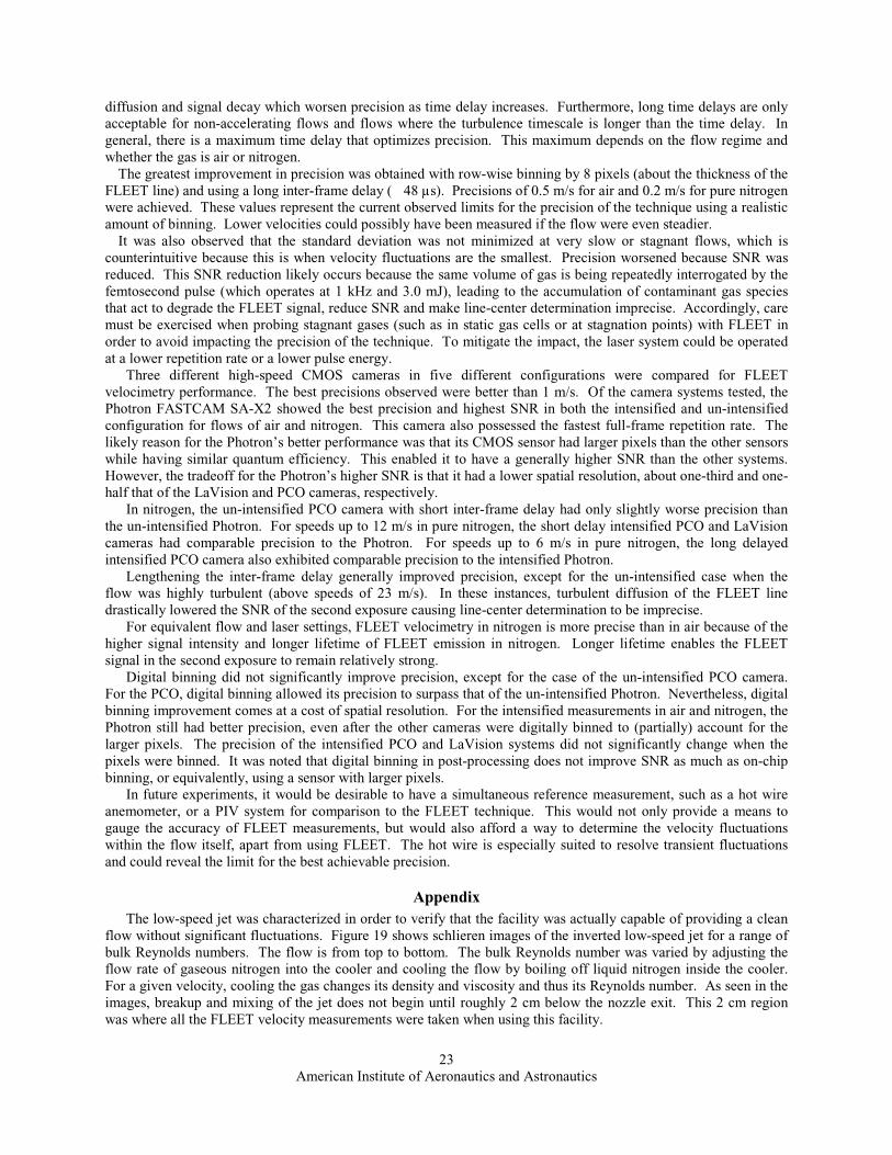
Appendix The low-speed jet was characterized in order to verify that the facility was actually capable of providing a clean

flow without significant fluctuations. Figure 19 shows schlieren images of the inverted low-speed jet for a range of bulk Reynolds numbers. The flow is from top to bottom. The bulk Reynolds number was varied by adjusting the flow rate of gaseous nitrogen into the cooler and cooling the flow by boiling off liquid nitrogen inside the cooler. For a given velocity, cooling the gas changes its density and viscosity and thus its Reynolds number. As seen in the images, breakup and mixing of the jet does not begin until roughly 2 cm below the nozzle exit. This 2 cm region was where all the FLEET velocity measurements were taken when using this facility.


24

Figure 19. Schlieren images of inverted low-speed jet with the nozzle exit at the top of the frame. Flow is top to bottom. Variation of bulk Reynolds number, based on the jet diameter, was achieved by adjusting the flow rate of gaseous nitrogen into the cooler and cooling the flow by boiling off liquid nitrogen inside the cooler. As seen in the images, breakup and mixing of the jet does not begin until roughly 2 cm below the nozzle exit.

Acknowledgments C. J. Peters was supported by a NASA Space Technology Research Fellowship. S. B. Jones was the technician

at NASA Langley and his help was greatly appreciated. The authors wish to thank R. A. Burns for assistance in reviewing the manuscript. Support for this project was obtained from the NASA Langley IRAD Program under the direction of M. R. Waszak. Note that NASA does not endorse any particular manufacturer of equipment used in this paper. The names of the manufacturers are included for clarity and the equipment tested was mainly chosen because of its availability. Equipment from other manufacturers may perform equally as well or better.

References

1Michael, J., Edwards, M., Dogariu, A. and Miles, R., “Femtosecond laser electronic excitation tagging for quantitative velocity imaging in air,” Applied Optics, Vol. 50, No. 26, pp. 5158-5162, 2011.

2Edwards, M. “Femtosecond Laser Electronic Excitation Tagging,” Undergraduate Senior Thesis, Princeton University, 2012.

3Miles, R., Edwards, M., Michael, J., Calvert, N. and Dogariu, A., “Femtosecond Laser Electronic Excitation Tagging (FLEET) for Imaging Flow Structure in Unseeded Hot or Cold Air or Nitrogen” in 51st AIAA Aerospace Sciences Meeting including the New Horizons Forum and Aerospace Exposition, Grapevine, Texas, 2013.

4DeLuca, N., Miles, R., Kulatilaka, W., Jiang, N., Gord, J., “Femtosecond Laser Electronic Excitation Tagging (FLEET) Fundamental Pulse Energy and Spectral Response” in 30th AIAA Aerodynamic Measurement Technology and Ground Testing Conference, Atlanta, Georgia, 2014.

5Edwards, M., Limbach, C., Miles, R. and Tropina, A., “Limitations on High-Spatial Resolution Measurements of Turbulence Using Femtosecond Laser Tagging” in 53rd AIAA Aerospace Sciences Meeting, Kissimmee, Florida, 2015.

6Calvert, N., Dogariu, A. and Miles, R., “FLEET Boundary Layer Velocity Profile Measurements” in 44th AIAA Plasmadynamics and Lasers Conference, San Diego, California, 2013.

7Miles, R., Cohen, C., Connors, J., Howard, P., Huang, S., Markovitz, E., Russell, G., “Velocity measurements by vibrational tagging and fluorescent probing of oxygen,” Optics Letters, Vol. 12, No. 11, pp. 861-863, 1987.

8Miles, R., Connors, J., Markovitz, E., Howard, P., Roth, G., “Instantaneous profiles and turbulence statistics of supersonic free shear layers by Raman excitation plus laser-induced electronic fluorescence (RELIEF) velocity tagging of oxygen,” Experiments in Fluids, Vol. 8, No. 1-2, pp. 17-24, 1989.

9Dam, N., Klein-Douwel, R., Sijtsema, N., ter Meulen, J., “Nitric oxide flow tagging in unseeded air,” Optics Letters, Vol. 26, No. 1, pp. 36-38, 2001.

10Pitz, R., Brown, T., Nandula, S., Skaggs, P., DeBarber, P., Brown, M., Segall, J., “Unseeded velocity measurement by ozone tagging velocimetry,” Optics Letters, Vol. 21, No. 10, pp. 755-757, 1996.

11Forkey, J., Lempert, W., Miles, R., “Accuracy limits for planar measurements of flow field velocity, temperature and pressure using Filtered Rayleigh Scattering,” Experiments in Fluids, Vol. 24, No. 2, pp. 151-162, 1998.

12Seasholtz, R., Zupanc, F., Schneider, S., “Spectrally resolved Rayleigh scattering diagnostic for hydrogen-oxygen rocket plume studies,” Journal of Propulsion and Power, Vol. 8, No. 5, pp. 935-942, 1992.

13Cummings, E., “Laser-induced thermal acoustics: simple accurate gas measurements,” Optics Letters, Vol. 19, No. 17, pp. 1361-1363, 1994.

14Taylor, J., An Introduction to Error Analysis: The Study of Uncertainties in Physical Measurements, 2nd ed., University Science Books, Sausalito, California, 1997, Chap. 3.

Flow

Documents

Precision of FLEET Velocimetry using High-Speed … of FLEET Velocimetry using High-Speed CMOS Camera Systems ... LaVision Imager scientific CMOS (sCMOS) and a Photron FASTCAM SA-X2,