Embed Size (px)
Citation preview

Predicting Deformations of Geosynthetic Reinforced Soil for Bridge Support
Monday, September 17, 20181:00-2:30 PM ET
TRANSPORTATION RESEARCH BOARD

The Transportation Research Board has met the standards and
requirements of the Registered Continuing Education Providers Program.
Credit earned on completion of this program will be reported to RCEP. A
certificate of completion will be issued to participants that have registered
and attended the entire session. As such, it does not include content that
may be deemed or construed to be an approval or endorsement by RCEP.

Purpose
Discuss design equations for predicting the maximum lateral deformation and settlement of geosynthetic reinforced soil (GRS) under various configurations and service loads.
Learning Objectives
At the end of this webinar, you will be able to:
• Apply design tools to deformation analysis of GRS bridge support systems
• Evaluate service limit state performance of bridge supports

Predicting Deformations of Geosynthetic
Reinforced Soil for Bridge Support
Moderator: Jennifer Nicks, PhD, PEChair, AFS70 (Geosynthetics)
Co-Sponsors: AFS10 (Transportation Earthworks)AFS70 (Geosynthetics)
September 17, 2018

Background
In 2014, the Federal Highway Administration (FHWA) issued a contract for a research project titled “Service Limit State Design and Analysis of Engineered Fills for Bridge Support”
Motivation for the study was the limited methods available to accurately estimate deformations of abutments and foundations built using engineered fills.
In this evaluation, engineered fills were defined as compacted granular fill with and without layered reinforced soil systems.

Objectives
Develop practice-ready design tools
to evaluate immediate and
secondary settlement and
lateral deformation of engineered fills
used for bridge support.
Determine the stress distribution as a function of
depth transferred by the engineered
fill to native foundation soils.

Limitations of the Study & Future Research Needs
Does not support metallically stabilized earth abutments
Rigid facing elements were not evaluated
Deformation equations were prepared assuming static load (no live load or thermal load)

TasksLiterature review and data search
Synthesis and Evaluation of The Service Limit State of Engineered Fills for Bridge Support (FHWA-HRT-15-080
Development of the research plan
Parametric study
Design analysis and recommendations
Final Report and Recommendations (not yet published)

Research Team
Principal Investigator: Dr. Ming Xiao (Penn State University)
Co-Principal Investigator: Dr. Tong Qiu (Penn State University)
Research Assistant: Dr. Mahsa Khosrojerdi (formerly Penn State University)
Consultant: Jim Withiam (D’Appolonia Engineering Division of Group
Technology, Inc.)

Predicting Deformations of Geosynthetic
Reinforced Soil for Bridge Support
Presented by:Ming Xiao, PhD, PE - Pennsylvania State UniversityTong Qiu , PhD, PE - Pennsylvania State University
Mahsa Khosrojerdi, PhD - Pennsylvania State University
Moderated by:Jennifer Nicks , PhD, PE- U.S. Department of Transportation
TRB WebinarSeptember 2018
2
Outline
Introduction
Available Methods to Predict GRS abutment Deformations
Numerical Model Development and Validation
Prediction Tools for GRS Abutment Deformation
Prediction Tools for RSF deformation
Conclusions

3
Conventional Bridge Foundation Systems
Engineered Fills Used for Bridge Support
Recreated after Anderson and Brabant (2010)
Nishida et al. (2012)Jones (1996)

4
Geosynthetic Reinforced Soil Integrated Bridge System (GRS-IBS)
GeogridGeotextile
https://www.ipwea.org
https://www.fhwa.dot.govhttps://www.fhwa.dot.gov

5
Advantages
Simple and rapid construction
Lower costs
Readily available material and
equipment
Constructability in any weather
condition
Easier maintenance
Environmental friendlyhttps://www.fhwa.dot.gov/

6
Limit States
Ultimate Limit State (ULS)Set of unacceptable conditions related to safety/danger, e.g.,
collapse.
Service Limit State (SLS)Set of unacceptable conditions related to performance, e.g.,
excessive settlement or tilt.
A condition beyond which the structure no longer fulfills therelevant design criteria.

7
Adams Method (Adams et al. 2002):
Predicting Lateral Deformations of GRS Abutments
FHWA Method (Christopher et al. 1990):
Geoservices Method (Giroud 1989):
CTI Method (Wu 1994):
Jewell-Milligan Method (Jewell and Milligan, 1989):
Wu Method (Wu et al. 2013):
471.945.3516.5725.4281.11234
+
−
+
−
=
HL
HL
HL
HL
Rδ
2Ld
hε
δ =
=
25.1H
dh εδ
( ) ( )
−+
−−
=∆ dsih zH
KP φψ 90tan
245tan
21
reinf
rm
( ) ( ) ( )
−+
−−
+−+=∆ dsi
vbvishi zH
KbSSqzK φψβδδγγ 90tan
245tan)tantan1(tan5.0
reinf
HDb
D vvolqL
,2=
8
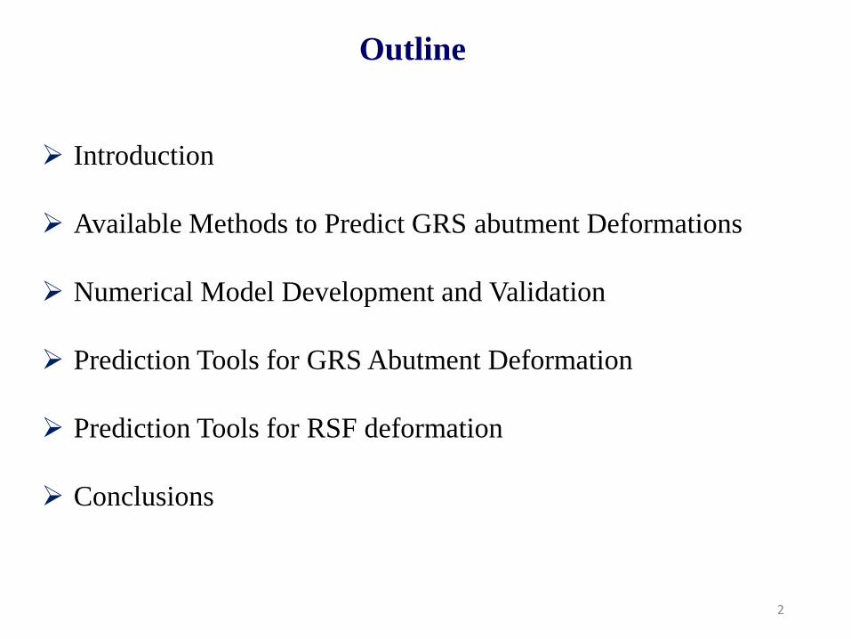
Predicting Maximum Settlement of GRS Abutments
Adams Method (Adams et al. 2011):
ρ = 3qb'
4πEGRS�12�1 +
a + b'2
b'2
� ln�H2+ �a + b'
2�2
�b'2�
2 �+12�1 −
a + b'2
b'2
� ln�H2 + a2
�b'2�
2 �+Ha
tan-1 �a + b'
H�+
Ha
tan-1 �-b'H��
ρ = Vertical displacement of GRS abutment
EGRS = Young’s modulus of the GRS composite
q = Applied pressure
a = Setback distance between the face of the wall and the applied load
b' = Width of facing block
H = Height of abutment
9
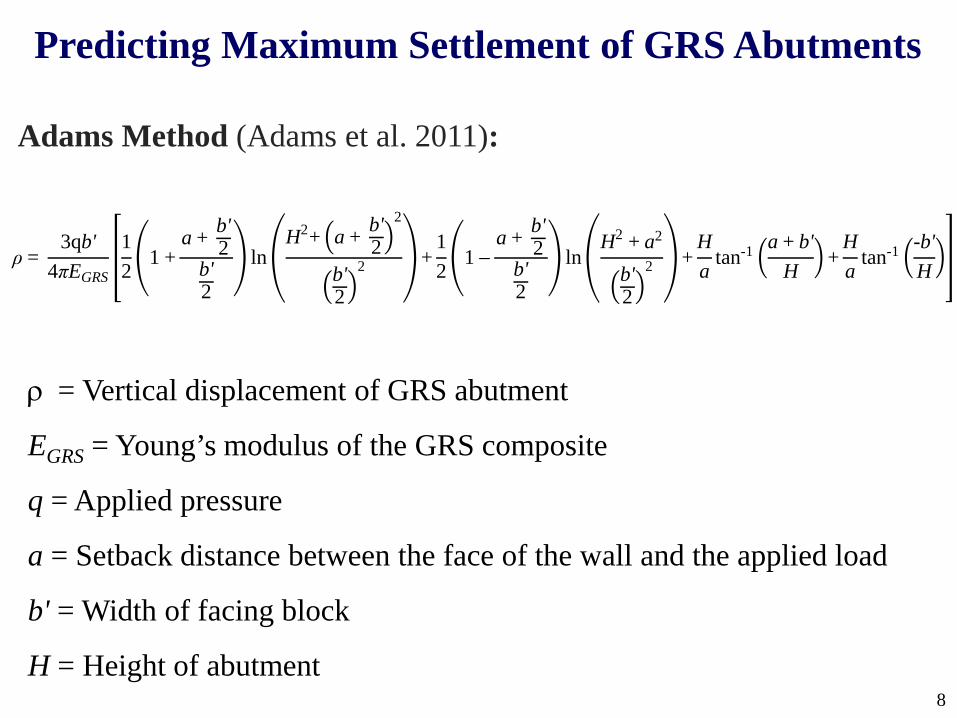
General Approach for Developing Prediction Tool
Model Calibration
and Validation
Parametric Study
Regression Analysis
Evaluating Prediction Equations

10
Numerical Modeling Using FLAC3D Software
Concrete SlabLinear Elastic
Material
Biaxial Woven GeotextileLinear Elastic-Plastic Material(Geogrid Structural Elements)
Concrete Modular Unit (CMU)Linear Elastic
Material
Compacted Backfill

11
Soil Constitutive Models
1. The elastic-perfectly plastic Mohr-Coulomb model
2. The Plastic Hardening model
3. The Plastic Hardening model combined with strain-softening
behavior

12
Model Calibration
-0.04
-0.02
0
0.02
0 0.05 0.1 0.15
Volu
met
ric S
train
(%)
Vertical Strain
σ'3=310 kPa
σ'3=103 kPa
σ'3=35 kPaExperimentModel IModel IIModel III
0
1000
2000
3000
0 0.05 0.1 0.15
Dev
iato
r Stre
ss (k
Pa)
Vertical Strain (%)
σ'3=310 kPa
σ'3=103 kPa
σ'3=35 kPa
ExperimentModel IModel IIModel III
Model Parameters Model I Model II Model
IIIMohr-Coulomb
ModelE 50 MPa N/A N/Aν 0.3 0.3 0.3φ 48° 48° 48°Ψ 7° 7° 7°c 27.6 kPa 27.6 kPa 27.6 kPa
Plastic Hardening Model
E50ref N/A 50 MPa 50 MPa
Pref N/A 100 100m N/A 0.5 0.5Rf N/A 0.8 0.8
Strain Softening Model
Residual friction angel
N/A N/A 38°
Residual dilation angel
N/A N/A 0°
Residual cohesion
N/A N/A 1.3 kPa
• Nicks el al. (2013) Experiment

13
Soil Constitutive Model: Plastic Hardening Model
f
fa R
qq =
m: Power coefficient for stress level dependency of stiffness
𝜎𝜎3′: Minor principal stress
Rf: Failure ratio, qf is the ultimate deviatory stress, and qa is:
𝐸𝐸50𝑟𝑟𝑟𝑟𝑟𝑟: Secant stiffness in standard drained triaxial test
m
refref
pcc
EE
+−
=φ
σφcot
'cot 35050
Shear yield function is defined as:
𝑓𝑓𝑠𝑠 =2𝐸𝐸𝑖𝑖
𝑞𝑞𝑞𝑞𝑎𝑎𝑞𝑞𝑎𝑎 − 𝑞𝑞
−𝑞𝑞
2𝐸𝐸50− 𝛾𝛾𝑝𝑝 = 0

14
Model Validation
Model ParametersPlastic Hardening Model Parameters
E50ref (MPa) 110
m (dimensionless) 0.5Rf (dimensionless) 0.75
Pref (kPa) 100(dimensionless) 0.3
Block-Block Interface PropertiesFriction angle (°) 57
Normal stiffness (kN/m/m) 1000×103
Shear stiffness (kN/m/m) 50×103
Soil-Block Interface PropertiesFriction angle (°) 44
Normal stiffness (kN/m/m) 100×103
Full-Scale GRS Wall Test by Bathurst et al. (2000)

15
Model Validation Full-Scale GRS Wall Test by Bathurst et al. (2000)
Geogrid Properties Walls 1 and 3 Wall 2
Reinforcement type PP PPAperture dimensions (mm) 25×33 25×69Ultimate strength (kN/m) 14 7
Initial stiffness (kN/m) 115 56.5

16
Multi-stage Construction Process in Numerical Model

0 2 4 6 8 10Lateral deformation (mm)
Wall 3
ExperimentalresultNumericalresult
0 10 20 30 40 50Lateral deformation
(mm)
0
1
2
3
4
0 2 4 6 8 10
Elev
atio
n (m
)
Lateral deformation (mm)
Wall 1
0 2 4 6 8 10Lateral deformation
(mm)
Wall 2
0
0.9
1.8
2.7
3.6
0 4 8 12 16
Elev
atio
n (m
)
Lateral deformation (mm)
30 kPa
0 20 40 60 80Lateral deformation
(mm)
wall1 (EXP)wall1 (NUM)wall2 (EXP)wall2 (NUM)
Lateral deformation of GRS walls under surcharge loads
Lateral deformation of GRS walls at the end of construction without surcharge
50 kPa 70 kPa
17

18
Parametric StudyParameters (unit) Values
Backfill properties Friction angle, φ (°) 40, 45, 46, 48, 50, 55
Reinforcement properties
Reinforcement spacing, Sv (m) 0.2, 0.4, 0.6, 0.8
Reinforcement length, LR0.4 , 0.5 , 0.7 ,
(H is height of abutment)
Reinforcement stiffness, J (kN/m) 500, 1000, 1500, 2000, 2500
Abutment geometry
Abutment height, H (m) 3, 4, 5, 6, 9Facing batter, β (°) 0, 2, 4, 8Concrete footing width, B (m) 0.5, 0.7, 1, 1.5, 2, 3
Surcharge load (kPa) 50, 100, 200, 400
Parameters Benchmark Values
Friction angle 48°Reinforcement length 2.5 m
Reinforcement stiffness 2000 kN/mReinforcement spacing 0.2 m
Abutment height 5 mFacing batter 2°

19
Parametric Study
Parametric study was conducted in two phases:
Phase 1: One of the parameters was changed.Objective: To obtain an initial understanding of the deformationvariation with one parameter when other parameters are fixed.A total of 172 simulations were conducted in Phase 1.
Phase 2: Parameters were varied simultaneously.Objective: To quantify the dependency between the parametersand their mutual effects on deformation.A total of 184 simulations were conducted in Phase 2.

20
Phase 1 of Parametric Study
0
10
20
30
40
40 45 50 55
Late
ral d
efor
mat
ion
(mm
)
Friction angle (deg)
50 kPa100 kPa200 kPa400 kPa
0
10
20
30
40
50
40 45 50 55
Settl
emen
t (m
m)
Friction angle (deg)
50 kPa100 kPa200 kPa400 kPa
0
20
40
60
80
0.2 0.4 0.6 0.8
Late
ral d
efor
mat
ion
(mm
)
Reinforcement spacing (m)
50 kPa100 kPa200 kPa400 kPa
0
20
40
60
80
0.2 0.4 0.6 0.8
Settl
emen
t (m
m)
Reinforcement spacing (m)
50 kPa100 kPa200 kPa400 kPa

21
Regression Analysis
The best prediction model:
Least root mean square error, RMSE value;
Highest coefficient of determination, R2 value;
Correct polarity for each ai coefficient.
In this equation, ∆GRS is the maximum lateral deformation or settlement of GRS abutment, ai are constant coefficients, xirepresent functions of input parameters which could have any format (i = 0 to 8).
88776655443322110 xaxaxaxaxaxaxaxaaGRS ++++++++=∆

22
First Try for Regression Model
∆𝐺𝐺𝐺𝐺𝐺𝐺= 𝑎𝑎0+𝑎𝑎1𝑞𝑞∗+𝑎𝑎2𝜙𝜙∗+𝑎𝑎3𝑆𝑆𝑣𝑣∗+𝑎𝑎4𝐽𝐽∗ +𝑎𝑎5 𝛽𝛽∗ + 𝑎𝑎6𝐻𝐻∗+𝑎𝑎7𝐿𝐿𝐺𝐺∗ +𝑎𝑎8𝐵𝐵∗
q*, φ*, Sv*, J*, β*, H*, LR* and B* are defining as q/q0, φ/φ0, Sv/ Sv0, J/J0,
β/β0, H/H0, LR/LR0 and B/B0, respectively.
In this study q0 = 200 kPa, Sv0 = 0.2 m, J0 = 500 kN/m, φ0 = 45°, β0= 90°,H0 = 5 m, LR0 =2.5 m and B0 =1 m.
q should be in the unit of kPa, φ and β should be in degree, J in kN/m, andSv , H, LR, and B should be in the unit of m, then ∆GRS result would be inm.

Prediction Eq. a0 a1 a2 a3 a4 a5 a6 a7 a8 R2 RMSE
Lateral deformation 0.019 7e-5 -7e-4 -5e-6 0.03 -9e-4 0.001 -8e-4 0.008 0.68 0.008
Settlement 0.038 8e-5 -1e-3 -5e-6 0.03 -9e-4 0.002 -7e-4 0.009 0.72 0.009
23
First Try for Regression Model
Model should have the least RMSE value and the closest R2 value to one!
The signs of a3 and a4 are not logical!
Model Predicts negative
deformation values!
∆𝐺𝐺𝐺𝐺𝐺𝐺= 𝑎𝑎0+𝑎𝑎1𝑞𝑞∗+𝑎𝑎2𝜙𝜙∗+𝑎𝑎3𝑆𝑆𝑣𝑣∗+𝑎𝑎4𝐽𝐽∗ +𝑎𝑎5 𝛽𝛽∗ + 𝑎𝑎6𝐻𝐻∗+𝑎𝑎7𝐿𝐿𝐺𝐺∗ +𝑎𝑎8𝐵𝐵∗

24
Developing Prediction Equation
The effects of individual variables on the deformation of GRSabutment, investigated through Phase 1, were studied to findfunctions for input parameters (xi).
• Reinforcement Stiffness:
0
0.01
0.02
0.03
0.04
0.05
500 1000 1500 2000 2500
Y
J
Y=J^(-0.7)Y=J^(-0.5)
→ Instead of using x4=J* in the first equation, it can be replaced by x4=𝑱𝑱∗
𝒂𝒂
0
10
20
30
40
50
500 1000 1500 2000 2500
Settl
emen
t (m
m)
Reinforcement stiffness (kN/m)
50 kPa100 kPa200 kPa

25
Tries for Nonlinear Regression Prediction Model
.
.
.
∆𝐺𝐺𝐺𝐺𝐺𝐺= 𝑎𝑎0 + 𝑎𝑎1𝑞𝑞∗ + 𝑎𝑎2 tan 90 + 𝜙𝜙 + 𝑎𝑎3𝑆𝑆𝑣𝑣∗ +𝑎𝑎4 𝐽𝐽∗ + 𝑎𝑎6 1 − 𝛽𝛽∗ + 𝑎𝑎7𝐻𝐻∗ + 𝑎𝑎8𝐿𝐿𝐺𝐺∗ +𝑎𝑎9 𝐵𝐵∗𝑎𝑎10
∆𝐺𝐺𝐺𝐺𝐺𝐺= 𝑎𝑎0 + 𝑎𝑎1𝑆𝑆𝑣𝑣∗
𝐽𝐽∗𝑎𝑎2𝑎𝑎3𝑞𝑞∗ + 𝑎𝑎4 tan 90 + 𝜙𝜙 + 𝑎𝑎5 1 − 𝛽𝛽∗ + 𝑎𝑎6𝐻𝐻∗ + 𝑎𝑎7𝐿𝐿𝐺𝐺∗ +𝑎𝑎8 𝐵𝐵∗
𝑎𝑎9
∆𝐺𝐺𝐺𝐺𝐺𝐺= 𝑎𝑎0 + 𝑎𝑎1𝑞𝑞𝑆𝑆𝑣𝑣∗
𝐽𝐽∗𝑎𝑎2× 𝐵𝐵∗𝑎𝑎3 𝑎𝑎4 tan 90 + 𝜙𝜙 + 𝑎𝑎5 1 − 𝛽𝛽∗ + 𝑎𝑎6𝐻𝐻∗ + 𝑎𝑎7𝐿𝐿𝐺𝐺∗
∆𝐺𝐺𝐺𝐺𝐺𝐺= 𝑎𝑎0 + 𝑎𝑎1𝑞𝑞∗𝑎𝑎2 × 𝑡𝑡𝑎𝑎𝑡𝑡2 90 + 𝜙𝜙 ×
𝑆𝑆𝑣𝑣∗
𝐽𝐽∗𝑎𝑎3× 𝐵𝐵∗𝑎𝑎4 𝑎𝑎5 1 − 𝛽𝛽∗ + 𝑎𝑎6𝐻𝐻∗ + 𝑎𝑎7𝐿𝐿𝐺𝐺∗
∆𝐺𝐺𝐺𝐺𝐺𝐺= 𝑎𝑎0 + 𝑎𝑎1𝑞𝑞∗𝑎𝑎2 × 𝑡𝑡𝑎𝑎𝑡𝑡2 90 + 𝜙𝜙 ×
𝑆𝑆𝑣𝑣∗
𝐽𝐽∗𝑎𝑎3× 𝐵𝐵∗𝑎𝑎4 𝑎𝑎5 1 − 𝛽𝛽∗ + 𝑎𝑎6𝐻𝐻∗ + 𝑎𝑎7
𝐿𝐿𝐺𝐺∗
𝐻𝐻∗
2
𝑆𝑆𝐺𝐺𝐺𝐺𝐺𝐺= 0.005 + 0.006 × 𝑞𝑞∗1.42 × 𝑡𝑡𝑎𝑎𝑡𝑡2 90 + 𝜙𝜙 ×
𝑆𝑆𝑣𝑣∗
𝐽𝐽∗0.49 × 𝐵𝐵∗1.26 −23.3 + 26.7 1 − 𝛽𝛽∗ + 0.025𝐻𝐻∗ − 0.2𝐿𝐿𝐺𝐺∗
𝐿𝐿𝐺𝐺𝐺𝐺𝐺𝐺= 0.056 × 𝑞𝑞∗1.32 × 𝑡𝑡𝑎𝑎𝑡𝑡2 90 + 𝜙𝜙 ×
𝑆𝑆𝑣𝑣∗
𝐽𝐽∗0.17 × 𝐵𝐵∗1.11 −1.53 + 1.69 1 − 𝛽𝛽∗ + 0.105𝐻𝐻∗ − 0.0125𝐿𝐿𝐺𝐺∗2

26
Prediction Models
R2=0.91 R2=0.88
𝐿𝐿𝐺𝐺𝐺𝐺𝐺𝐺= 0.056 × 𝑞𝑞∗1.32 × 𝑡𝑡𝑎𝑎𝑡𝑡2 90 + 𝜙𝜙 ×
𝑆𝑆𝑣𝑣∗
𝐽𝐽∗0.17 × 𝐵𝐵∗1.11 −1.53 + 1.69 1 − 𝛽𝛽∗ + 0.105𝐻𝐻∗ − 0.0125𝐿𝐿𝐺𝐺∗2
𝑆𝑆𝐺𝐺𝐺𝐺𝐺𝐺= 0.005 + 0.006 × 𝑞𝑞∗1.42 × 𝑡𝑡𝑎𝑎𝑡𝑡2 90 + 𝜙𝜙 ×
𝑆𝑆𝑣𝑣∗
𝐽𝐽∗0.49 × 𝐵𝐵∗1.26 −23.3 + 26.7 1 − 𝛽𝛽∗ + 0.025𝐻𝐻∗ − 0.2𝐿𝐿𝐺𝐺∗

27
Evaluation of Prediction Equation of Settlement of GRS Abutment
Set No. Reference φ(°)
J(kN/m)
Sv(m)
B(m)
β(°)
H(m)
LR(m)
1 Helwany et al. (2007) 34.8 800 0.2 0.9 0 4.65 3.15
2 Helwany et al. (2007) 34.8 380 0.2 0.9 0 4.65 3.15
3 Hatami and Bathurst (2005) 40 115 0.6 6.0 8 3.6 2.5
4 Hatami and Bathurst (2005) 40 56.5 0.6 6.0 8 3.6 2.5
5 Gotteland et al. (1997) 30 340 0.6 1.0 8 4.35 2.4
Set No. Load (kPa)
Actual value(mm)
This study FHWA Method∆ (mm) Error (%) ∆ (mm) Error (%)
1
100 15 16 6.7 6.7 -55.3200 33 32 -3.0 13.5 -59.1300 55 54 -1.8 20.2 -63.3400 75 79 5.3 27.0 -64.0500 97 105 8.2 33.7 -65.3
2
100 23 20 -13.0 6.7 -70.9200 57 44 -22.8 13.5 -76.3300 100 74 -26.0 20.2 -79.8400 155 110 -29.0 27.0 -82.6
5 123 33 32 -3.0 8.4 -74.5

28
Evaluation of Prediction Equation of Lateral Deformation
Set No
Load (kPa)
Actual value(mm)
This study FHWA method
Geoservicemethod
CTI method
Jewell-Milligan method
Wu method Adams method
∆(mm)
Error(%)
∆(mm)
Error(%)
∆(mm)
Error(%)
∆(mm)
Error(%)
∆(mm)
Error(%)
∆(mm)
Error(%)
∆(mm)
Error(%)
1307 24 40 40.0 307 1179.2 - - - - - - - - 16 -33.3475 57 71 19.7 465 715.8 - - - - - - - - 42 -26.3
2214 36 28 -28.6 244 577.8 - - - - - - - - 27 -25.0317 61 48 -27.1 331 442.6 - - - - - - - - 45 -26.2414 115 68 -69.1 413 259.1 - - - - - - - - 69 -40.0
330 9 13 30.8 68 655.6 - - - - 31 242.2 7.3 -18.9 - -50 21 26 19.2 81 285.7 - - - - 38 79.0 17 -19.0 - -70 37 40 7.5 93 151.4 - - - - 44 20.0 31 -16.2 - -
430 12 15 20.0 68 466.7 - - - - 62 413.3 15 25.0 - -50 37 30 -23.3 81 118.9 - - - - 75 103.2 34 -8.1 - -70 58 47 -23.4 93 60.3 - - - - 89 53.1 61 5.2 - -
5 190 83 46 -80.4 264 218.1 111 33.7 180 116.9 - - - - - -

29
Incremental Sensitivity Analysis
)()()(
)()()(
1
1
xxxxxx
xyxyxy
SR
i
ii
i
ii
−
−
=+
+where yi+1(x) = equation output in step i+1due to variable x; yi(x) = equation output instep i due to variable x; xi+1(x) = value ofvariable x in step i+1; and xi(x)= value ofvariable x in step i.
0
2
4
6
8
10
12
14
0 5 10 15 20
Late
ral D
efor
mat
ion
(mm
)
Total Number of Increments
Friction angle

30
Incremental Sensitivity Analysis
0
5
10
15
20
25
30
0 10 20
Late
ral D
efor
mat
ion
(mm
)
Total Number of Increments
Friction angle
Reinforcement stiffness
Reinforcement spacing
Facing batter
Height
Reinforcement length
Foundation width
05
101520253035
0 10 20
Settl
emen
t (m
m)
Total Number of Increments
Friction angle
Reinforcement stiffness
Reinforcement spacing
Facing batter
Height
Reinforcement length
Foundation width
ParametersSR
Lateral Deformation Settlement
Friction angle -3.26 -1.71Reinforcement
spacing 1.00 0.69
Footing width 0.90 1.20
Abutment height 0.50 0.25
Facing batter -0.45 -0.20Reinforcement
length -0.33 -0.13
Reinforcement stiffness -0.16 -0.25

31
Tool Development

32
Deformations and Vertical Stress Distribution under 200 kPa Applied Pressure
Reinforcement spacing = 0.2 m Reinforcement spacing = 0.8 m
Max. Lateral Deformation= 9 mm
Max. Settlement=12 mm Max. Settlement=31mm
Max. Lateral Deformation= 34 mm

33
Reinforcement spacing = 0.2 m Reinforcement spacing = 0.8 m
0
1
2
3
4
5
0 100 200 300 400
Hei
ght o
f abu
tmen
t (m
)
Vertical stress (kPa)
Under 200 kPapressureGeostatic stress
0
1
2
3
4
5
0 100 200 300 400
Hei
ght o
f abu
tmen
t (m
)
Vertical stress (kPa)
Under 200 kPapressureGeostatic stress
Deformations and Vertical Stress Distribution under 200 kPa applied pressure
Max. vertical stress= 370 kPa Max. vertical stress= 470 kPa

34
Reinforced Soil Foundation (RSF)
Methods to predict the settlement of footings placed on unreinforced granular soil:• Modified Schmertmann• Hough • Peck and Bazaraa• Burland and Burbidge • D’Appolonia

35
Model Validation - Adams and Collin (1997) Experiments
Type Biaxial geogridUltimate strength 34 kN/m
Tensile strength in machine direction at 5% strain 20 kN/mTensile strength in cross machine direction at 5%
strain 25 kN/m
Vertical spacing of reinforcement 0.15 m Embedment depth of top geogrid layer 0.15 m
Apparatus size 25 mm × 30 mm

36
Model Validation
0
20
40
60
80
0 100 200 300 400 500 600
Settl
emen
t (m
m)
Applied Pressure (kPa)
Unreinforced-EXPReinforced-EXPUnreinforced-NUMReinforced-NUM

37
Parametric StudyParameters (unit) Values
Backfill properties
Friction angle, φ (deg) 30, 35, 40, 45, 50
Cohesion, c (kPa) 0, 1, 5, 10
Reinforcement properties
Reinforcement spacing, Sv(m) 0.2, 0.3, 0.4
Number of reinforcement layers, N 2, 3, 4,5
Reinforcement length extended beyond foundation, LX (m)
0.25B, 0.5B,
0.75B, B
Compacted depth, Dc (m) 0.9, 1.2, 1.5. 1.8
Reinforcement stiffness, J(kN/m)
500, 1000, 2000, 3000
Foundation dimension
Width of foundation, B (m) 1, 2, 3Length of foundation, L (m)
1B, 2B, 3B, 7B, 10B
Service load (kPa)50, 100,
200, 400, 600
Parametric study was conductedin two phases:
Phase 1: One of parameterschanges; a total of 135simulations was conducted inPhase 1.
Phase 2: Parameters are variedsimultaneously; a total of 175simulations was conducted inPhase 2.

38
NaLaLaBaDaSaJacaaqaaS XcvRSF 109876543210 )90tan( +++++++++++= φ
( )NaLaLaBaDaSaJacaaqaS Xcva
RSF 10987654320 )90tan(1 +++++++++××= φ
( )NaLaLaBaDaSaJacaqaS Xcva
RSF 987654320 )90tan(1 +++++++×+××= φ
( )NaLaLaBaDaSaJacaqaS Xcva
RSF 987654322
0 )90(tan1 +++++++×+××= φ
( )( )8765432
20 /)90(tan1 a
cva
RSF NLaBaDaJSacaaqaS ++++++×+××= φ
( ) ( )( )xcvaaa
RSF LaBaDaJSacaaNLBqaS 9876542
0 /)90(tan 321 +++++××+××= φ
Tries for Nonlinear Regression Prediction Model
SRSF = 1.3 × 10⁻³ × 𝑞𝑞∗1.17 × 𝑐𝑐𝑐𝑐𝑡𝑡2𝜙𝜙 × 𝑁𝑁−0.05 × (−0.07 −

39
0
0.01
0.02
0.03
0.04
0 0.01 0.02 0.03 0.04
Pred
icte
d (m
)
Simulation (m)
R2 = 0.9171
Equation for Predicting Settlement of RSF
SRSF = 1.3 × 10⁻³ × 𝑞𝑞∗1.17 × 𝑐𝑐𝑐𝑐𝑡𝑡2𝜙𝜙 × 𝑁𝑁−0.05 × (−0.07 − 6.5 × 10⁻⁵𝑐𝑐∗ +67.9( ⁄𝑆𝑆𝑣𝑣∗ 𝐽𝐽∗) +
q*, c*, J*, Sv*, Dc*, B*, L*, and Lx* are defined as q/q0,
c/c0, J/J0, Sv/ Sv0, Dc/Dc0, B/B0, L/L0, and LX/LX0
respectively.
q and c should be in the unit of kPa, φ in degree, J in
kN/m, and Sv, Dc, B, L and LX in the unit of m, then SRSF
result would be in m.
In this study q0 = 100 kPa, c0 = 1 kPa, J0 = 100 kN/m, Sv0
= 0.1 m, Dc0 = 1 m, B0 = 1 m, L0 = 1 m and LX0 = 1 m.

40
Evaluation of RSF Settlement Prediction EquationReference Set
No.φ(°)
c (kPa)
J(kN/m)
Sv(m)
Dc(m)
B(m)
L(m) N
Adams and Collin (1997) 1 36 1 450 0.15 5.55 0.91 0.91 3
Chen and Abu-Farsakh (2011) 2 25 13 370 0.607 4.86 1.822 1.822 4
Abu-Farsakh et al. (2013) 3 46 1 365 0.051 0.75 0.152 0.152 3
Set No. Load (kPa) ActualSettlement (mm)
PredictedSettlement (mm)
Error(%)
1
100 2.94 2.45 -17200 5.87 5.50 -6300 8.12 8.83 9400 11.06 12.36 12500 15.72 16.04 2600 22.46 19.84 -12
2
100 11.89 12.49 5200 25.79 28.07 9300 40.79 45.07 10400 60.72 63.06 4500 83.95 81.84 -3600 109.19 101.26 -7
3
100 0.36 0.19 -47200 0.73 0.43 -41300 1.2 0.69 -43400 1.51 0.97 -36500 1.83 1.26 -31600 2.24 1.55 -31
B = 0.91 m
B = 1.822 m
B = 0.152 m

41
Incremental Sensitivity Analysis
1
2
3
4
5
0 5 10 15 20
RSF
Set
tlem
ent (
mm
)
Total Number of Increments
Friction Angle
Cohesion
Reinforcement Stiffness
Reinforcement Spacing
Compacted Depth
Foundation Width
Foundation Length
Number of Reinforcement
Parameters SRFriction angle -2.7
Reinforcement spacing 0.52Compacted depth 0.39
Reinforcement stiffness -0.34Width of foundation 0.32Length of foundation 0.10
Number of reinforcement -0.05Cohesion -0.01

42
Conclusions
The Plastic Hardening model can accurately predict the behavior
of soil in simulation of GRS abutments and RSF under service
loads.
This study suggests these equations for calculating the maximum
lateral deformation and settlement of GRS abutment and
maximum settlement of RSF under service loads:
𝑆𝑆𝐺𝐺𝐺𝐺𝐺𝐺 = 0.005 + 0.006 × 𝑞𝑞∗1.42 × 𝑡𝑡𝑎𝑎𝑡𝑡2 90 + 𝜙𝜙 ×𝑆𝑆𝑣𝑣∗
𝐽𝐽∗0.49 × 𝐵𝐵∗1.26 −23.3 + 26.7 1 − 𝛽𝛽∗ + 0.025𝐻𝐻∗ − 0.2𝐿𝐿𝐺𝐺∗
𝐿𝐿𝐺𝐺𝐺𝐺𝐺𝐺 = 0.056 × 𝑞𝑞∗1.32 × 𝑡𝑡𝑎𝑎𝑡𝑡2 90 + 𝜙𝜙 ×𝑆𝑆𝑣𝑣∗
𝐽𝐽∗0.17 × 𝐵𝐵∗1.11 −1.53 + 1.69 1 − 𝛽𝛽∗ + 0.105𝐻𝐻∗ − 0.0125𝐿𝐿𝐺𝐺∗2
SRSF = 1.3 × 10⁻³ × 𝑞𝑞∗1.17 × 𝑐𝑐𝑐𝑐𝑡𝑡2𝜙𝜙 × 𝑁𝑁−0.05 × (−0.07 − 6.5 × 10⁻⁵𝑐𝑐∗ +67.9( ⁄𝑆𝑆𝑣𝑣∗ 𝐽𝐽∗) + 0.15𝐷𝐷𝑐𝑐∗ + 0.06𝐵𝐵∗ +

43
Conclusions
Results of sensitivity analysis for suggested equations indicated
that:
In GRS abutment lateral deformation equation, soil friction
angle and reinforcement spacing have the highest effect;
In GRS abutment settlement equation, soil friction angle
and foundation width have the highest effect;
In RSF settlement equation, soil friction angle and
reinforcement spacing have the highest effect.

Today’s Speakers• Jennifer Nicks, FederalHighway Administration, [email protected]• Ming Xiao, Penn State University,
[email protected]• Tong Qiu, Penn State University,
[email protected]• Mahsa Khosrojerdi, Arup,

Get Involved with TRB• Getting involved is free!• Join a Standing Committee (http://bit.ly/2jYRrF6)• Become a Friend of a Committee
(http://bit.ly/TRBcommittees)– Networking opportunities– May provide a path to become a Standing Committee
member– Sponsoring Committees: AFS10, AFS70
• For more information: www.mytrb.org– Create your account– Update your profile

Receiving PDH credits
• Must register as an individual to receive credits (no group credits)
• Credits will be reported two to three business days after the webinar
• You will be able to retrieve your certificate from RCEP within one week of the webinar