Embed Size (px)
Citation preview
University of Rhode Island University of Rhode Island
DigitalCommons@URI DigitalCommons@URI
Environmental and Natural Resource Economics Faculty Publications
Environmental and Natural Resource Economics
2016
Predicting human cooperation in the Prisoner’s Dilemma using Predicting human cooperation in the Prisoner’s Dilemma using
case-based decision theory case-based decision theory
Todd Guilfoos
Andreas D. Pape
Follow this and additional works at: https://digitalcommons.uri.edu/enre_facpubs
The University of Rhode Island Faculty have made this article openly available. The University of Rhode Island Faculty have made this article openly available. Please let us knowPlease let us know how Open Access to this research benefits you. how Open Access to this research benefits you.
This is a pre-publication author manuscript of the final, published article.
Terms of Use This article is made available under the terms and conditions applicable towards Open Access
Policy Articles, as set forth in our Terms of Use.
Noname manuscript No.(will be inserted by the editor)
Predicting Human Cooperation in the Prisoner’s Dilemma Using Case-based
Decision Theory
Todd Guilfoos · Andreas Duus Pape
Received: date / Accepted: date
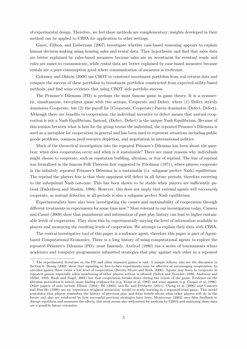
Abstract In this paper we show Case-based Decision Theory (Gilboa and Schmeidler, 1995) can explain
the aggregate dynamics of cooperation in the repeated Prisoner’s Dilemma, as observed in the experi-
ments performed by Camera and Casari (2009). Moreover, we find CBDT provides a better fit to the
dynamics of cooperation than does the existing Probit model, which is the first time such a result has
been found. We also find that humans aspire to a payoff above the mutual defection outcome but below
the mutual cooperation outcome, which suggests they hope, but are not confident, that cooperation can
be achieved. Finally, our best-fitting parameters suggest that circumstances with more details are easier
to recall. We make a prediction for future experiments: if the repeated PD were run for more periods, that
we would be begin to see an increase in cooperation, most dramatically in the second treatment, where
history is observed but identities are not. This is the first application of Case-based Decision Theory to
a strategic context and the first empirical test of CBDT in such a context. It is also the first application
of bootstrapped standard errors to an agent-based model.
JEL codes: D01, D83, C63, C72, C88
Keywords Case-based Decision Theory · Prisoner’s Dilemma · Learning · Agent-based Computational
Economics · Experimental Economics
The order of the authors is not indicative of effort or contribution towards this article.
T. GuilfoosDepartment of Environmental and Natural Resource Economics, University of Rhode Island, 219 Coastal Institute, 1Greenhouse Road, Kingston, RI 02881E-mail: [email protected]
A. D. PapeEconomics Department, Binghamton University, PO Box 6000, Binghamton NY, 13902Phone: 607-777-2660 Fax: 607-777-2681E-mail: [email protected]
1 Introduction
In this paper, we use Case-based Decision Theory (Gilboa and Schmeidler, 1995) to explain experimental
data of human behavior in the repeated Prisoner’s Dilemma game. We find that the aggregate dynamics
of cooperation are predicted by this theory. We fit the parameters of the model to data and establish
that all parameters are statistically significant. We establish this fact by comparing experimental data
collected by Camera and Casari (2009) against simulated data generated by a computer program called
the Case-based Software Agent (CBSA). CBSA was introduced in Pape and Kurtz (2013), who show
that CBSA (and therefore Case-based Decision Theory) explains individual human behavior in a series of
classification learning experiments from Psychology starting with Shepard, Hovland, and Jenkins (1961).
Here we show that CBSA can explain human group behavior in a setting that is dynamic and strategic.
Case-based Decision Theory is a mathematical model of choice under uncertainty which has the
following primitives: A set of problems or circumstances that the agent faces; a set of actions that the
agent can choose in response to these problems; and a set of results which occur when an action is applied
to a problem. Together, a problem, action, and result triplet is called a case, and can be thought of as one
complete learning experience. The agent has a finite set of cases, called a memory, which it consults when
making new decisions. The Case-based Software Agent is a software agent, i.e. “an encapsulated piece of
software that includes data together with behavioral methods that act on these data (Tesfatsion, 2006).”
CBSA computes choice data consistent with an instance of CBDT for an arbitrary choice problem or
game, provided that the problem is well-defined and sufficiently bounded.
We analyze data from an experiment by Camera and Casari (2009), in which study subjects are
grouped into small ‘economies’ to play the repeated Prisoner’s Dilemma. The purpose of their exper-
iment is to vary the level of information available to players about each other and measure the effect
on cooperation. For example, in one treatment, the players are supplied unique identifiers for their
opponents, so they know when they encounter the same opponent again. Because CBDT encodes the
agent’s information about the current choice directly (in the aforementioned “problem” variable), this is
a particularly appropriate experiment to test with CBSA. We compare simulated data to real data by
measuring the mean squared difference in probability of cooperation over time. Like regression analysis,
we then search the space of free parameter values for those that provide the best fit (minimizing mean
squared error).1 Moreover, we establish the precision by which we are able to estimate these parameters
by bootstrapping standard errors, which is a first for agent-based models.
We are able to establish four key facts about CBDT and its relationship with human choice behavior
in Camera and Casari’s Prisoner’s Dilemma experiment. We find:
(1) The choice behavior of this software agent (and therefore Case-based Decision Theory) correctly
predicts the empirically observed trajectory of average cooperation rates over time across three different
treatments. This shows that CBDT can predict human behavior in a strategic and dynamic setting.
(2) The choice behavior implied by CBSA is a closer fit to the empirical data than the best-fitting
Probit model (from Camera and Casari’s paper), and CBSA has only a fifth as many parameters to fit to
data. This is a vote in favor of CBSA as a useful empirical description of human behavior in the repeated
Prisoner’s Dilemma and is a novel result in the literature.
(3) The best-fitting CBSA parameters suggest humans aspire to a payoff value above the mutual
defection payoff but below the mutual cooperation payoff, which suggests they hope, but are not confident,
that cooperation can be achieved. In principle, the best-fitting aspiration values could have fallen into
1 The free parameters of CBSA include two kinds of forgetfulness and an aspiration level. See Section 3 for details.
2
the ‘unreasonable’ range: namely greater than the best or lower than the worst possible payoff. The fact
that this did not happen serves as an specification test of CBSA.2
(4) Circumstances with more details are easier to recall. The evidence is that our best-fitting level of
recall probability increases as the experimental treatment varies as to share more information with the
agents.
These findings are useful in understanding the behavior of human subjects as well as developing
a framework in which we can predict human behavior. For example, the infinitely iterated prisoner’s
dilemma can sustain cooperation when sufficiently-patient agents employ the ‘grim’ strategy, defecting
forever if their partner defects, but this strategy does not seem to be played by human subjects. This
paper can be thought of as part of an effort to find alternative, empirically valid explanations of decision-
making in this strategic context.
Below, we first review the relevant literature in decision theory, game theory, and the empirical
study of the Prisoner’s Dilemma (Section 2). Second, we describe the experiment of Camera and Casari
(2009) and explain how we simulate this experiment it in the Case-based Software Agent framework,
which implements Case-based Decision Theory (Section 3). Third, we describe our statistical method
of finding the best-fitting parameters of CBSA to match the human data, including how we bootstrap
standard errors of our parameter estimates (Section 4). Fourth, we present and discuss our empirical
results (Section 5), and, in Section 6, we discuss the implications of these results for case-based decision
theory. In Section 7, we conclude.
2 Related Literature
The central investigative tool of this paper is the Case-based Software Agent (CBSA). It is a compu-
tational implementation of Case-Based Decision Theory (CBDT) introduced in Gilboa and Schmeidler
(1995). Implementations produce agent choice behavior given a mathematical representation in the tradi-
tion of von Neumann and Morgenstern (1944) and Savage (1954). Designed correctly, the choice behavior
produced by an implementation can be directly compared to empirical choice data of the same prob-
lem faced by humans. This can yield two classes of insights: First, the comparison can shed light on
the question of whether and in what ways CBSA (and therefore CBDT) serves as a representation or
‘explanation’ of human behavior. Second, the comparison can shed light on the empirical phenomenon
itself: for example, we learn what level of forgetfulness is consistent with the human behavior observed
in the experiments found in Camera and Casari (2009).
CBDT postulates that when an agent is confronted with a new problem, she asks herself: How similar
is today’s case to cases in memory? What acts were taken in those cases? What were results? She then
forecasts payoffs of actions using her memory, and chooses the action with the highest forecasted payoff.
The primitives are: a finite set of problems P, a finite set of acts A, and a set of results R. A case is a
triplet consisting of a problem, the act taken, and the outcome (result) of that act given the problem. A
case can be thought of as a single, complete learning experience. The set of all cases is C = P ×A×R.
CBDT representations are defined by four additional components. The first component of a CBDT
representation is the agent’s memory. Memory is a set of cases which, in CBSA, can be thought of as the
list of learning experiences the agent has had. An agent’s memory is denotedM. The second component
is the utility function u : R → R. It is defined in the usual way. The third component is the similarity
2 Like other specification tests, passing the test does not mean that the model is necessarily correctly specified; only thatfailing the test would have been evidence that it is misspecified.
3

function s : P×P → [0, 1]. The output value of the similarity function gives how much the input problems
resemble each other in the opinion of the agent. The fourth component is the aspiration level H ∈ R. It
is a reference level of utility, like expected value. However, while an expected value is the level of utility
one believes on average is the most likely, the aspiration level should be thought of as the agent’s target
level of utility, which could, in principle, differ from the expected value. Mechanistically, it serves as a
default value for forecasting utility of new alternatives. It also serves as a satificing level in the sense
of Simon (1957): “Behaviorally, H defines a level of utility beyond which the [decision maker] does not
appear to experiment with new alternatives (Gilboa and Schmeidler, 1996, page 2).”
Together, these four components define case-based utility:
CBU(a) =∑
(q,a,r)∈M(a)
s(p, q) [u(r)−H]
WhereM(a) is defined as the subset of the agents’ memoryM in which action a was taken. This utility
represents the agent’s preference in the sense that, for a fixed memory M, a is strictly preferred to a′ if
and only if CBU(a) > CBU(a′).
Case-based Decision Theory was introduced for the main purpose of disposing of the state space: that
is, the assumption that agents are able to list and reason about the set of all possible scenarios. CBDT
limits the set the agent must reason about to the set of past experiences, and requires only that the
agent be able to make similarity judgements between past experiences and new experiences. Therefore
CBDT naturally incorporates cognitive constraints. Moreover, the implementation of CBSA here in this
paper also includes forgetfulness explicitly.3
This paper contributes to a growing empirical literature testing the explanatory power of CBDT;
these papers generally find support for it.
In the paper most closely related to this one, Pape and Kurtz (2013) introduce CBSA and find
that imperfect memory, accumulative (not average) utility, a similarity function consistent with research
from psychology, and a 80 − 85% target success rate renders CBSA a good fit for human data in the
classification learning experiment from the psychology literature.4
Ossadnik, Wilmsmann, and Niemann (2012) run a repeated choice experiment involving unknown
proportions of colored and numbered balls in urns, which is the canonical ambiguous choice setting (i.e.
Ellsberg, 1961). (The authors of CBDT suspect that it is a better model of human behavior in settings
of ambiguity versus risk.) Ossadnik et al (2012) find that CBDT explains these data well compared to
alternatives such as minimax (Luce and Raiffa, 1957) and reinforcement learning (Roth and Erev, 1995a).
Their method has some similarities with CBSA, in that they choose parameter values and functional
forms of CBDT and calculate CBDT-governed agents’ optimal choices, and compare those choices to
aggregate human data. There are two important ways that the method differs from CBSA. First of all,
the CBSA method sweeps parameter values, so provides many more candidate values for fitting the
human data. Second, CBSA integrates forgetfulness and similarity functional forms from psychology.
Bleichrodt, Filko, Kothiyal, and Wakker (2012) provide a method to measure similarity weights which
avoids parametric assumptions about the weights. Their method has a number of advantages, including
testing CBDT in more generality. An advantage of the CBSA approach is the ability to predict CBDT-
governed behavior on arbitrary settings; the Bleichrodt et al (2012) approach implies a particular kind
3 Incorporating cognitive constraints into economic models is a hallmark of work in the intersection of economics andpsychology, such as Simon (1957), Simon, Egidi, and Marris (2008), Tyson (2008), Hanoch (2002), Ballinger, Hudson,Karkoviata, and Wilcox (2011), and Cappelletti, Guth, and Ploner (2011).
4 In particular, the ‘SHJ’ series of classification learning experiments, starting with Shepard, Hovland, and Jenkins (1961)and including Nosofsky (1986) and Nosofsky et al (1994).
4
of experimental design. Therefore, we feel these methods are complementary: insights developed in their
method can be applied to CBSA for application to other settings.
Gayer, Gilboa, and Lieberman (2007) investigate whether case-based reasoning appears to explain
human decision-making using housing sales and rental data. They hypothesize and find that sales data
are better explained by rules-based measures because sales are an investment for eventual resale and
rules are easier to communicate, while rental data are better explained by case-based measures because
rentals are a pure consumption good where communication of measures is irrelevant.
Golosnoy and Okhrin (2008) use CBDT to construct investment portfolios from real returns data and
compare the success of these portfolios to investment portfolios constructed from expected-utility-based
methods, and find some evidence that using CBDT aids portfolio success.
The Prisoner’s Dilemma (PD) is perhaps the most famous game in game theory. It is a symmet-
ric, simultaneous, two-player game with two actions, Cooperate and Defect, where (1) Defect strictly
dominates Cooperate, but (2) the payoff for (Cooperate, Cooperate) Pareto dominates (Defect, Defect).
Although there are benefits to cooperation, the individual incentive to defect means that mutual coop-
eration is not a Nash Equilibrium. Instead, (Defect, Defect) is the unique Nash Equilibrium. Because of
this tension between what is best for the group versus the individual, the repeated Prisoner’s Dilemma is
used as a metaphor for cooperation in general and has been used to represent situations including public
goods problems, common pool resource depletion, and negotiation in international politics.
Much of the theoretical investigation into the repeated Prisoner’s Dilemma has been about the ques-
tion: when does cooperation occur and when is it sustainable? There are many reasons why individuals
might choose to cooperate, such as reputation building, altruism, or fear of reprisal. The fear of reprisal
was formalized in the famous Folk Theorem first suggested by Friedman (1971), where players cooperate
in the infinitely repeated Prisoner’s Dilemma in a sustainable (i.e. subgame perfect Nash) equilibrium.
The reprisal the players fear is that their opponent will defect in all future periods, therefore reverting
to the suboptimal Nash outcome. This has been shown to be stable when players are sufficiently pa-
tient (Fudenberg and Maskin, 1986). However, this does not imply that rational agents will necessarily
cooperate, as mutual defection in all periods is also a subgame perfect Nash equilibrium.
Experimentalists have also been investigating the causes and sustainability of cooperation through
different treatments in experiments for some time now.5 Most relevant to our investigation today, Camera
and Casari (2009) show that punishment and information of past play history can lead to higher sustain-
able levels of cooperation. They show this by experimentally varying the level of information available to
players and measuring the resulting levels of cooperation. We attempt to explain their data with CBSA.
The central investigative tool of this paper is a software agent, therefore this paper is part of Agent-
based Computational Economics. There is a long history of using computational agents to explore the
repeated Prisoner’s Dilemma (PD): most famously, Axelrod (1980) ran a series of tournaments where
academics and computer programmers submitted strategies that play against each other in a repeated
5 The experimental literature on the PD and other repeated games is vast. A sample follows; also see the discussion inSection 6. Brosig (2002) show that signaling in face-to-face experiments may be effective at encouraging cooperation. Inone-shot games there exists a low level of cooperation (Bereby-Meyer and Roth, 2006). Agents may learn to cooperate inrepeated games, especially when monitoring of other players actions is allowed (Selten and Stoecker, 1986; Andreoni andMiller, 1993; Hauk and Nagel, 2001) but that cooperation breaks down during the course of the game. Evidence on thealtruism motivation is mixed, some finding evidence for (e.g. Kreps et al, 1982) and some against (e.g. Cooper et al, 1996).Other papers of note include Ellison (1994); Bo (2005) and Bo and Frechette (2011). Chong et al (2006) and Camererand Hua Ho (1999) use an ‘experience weighted attraction’ model to study learning in a repeated trust game. This modelpostulates that players remember the history of previous play and form beliefs about what other players will do in thefuture and also are reinforced by how successful previous strategies have been. Monterosso (2002) uses false feedback todisrupt equilibria and measures the effects; this work seems also well-suited for analysis by CBSA and analyzing these dataare a possible future extension.
5
PD in one of the earliest and most famous agent-based investigations. Similarly, Miller (1996) explores
the evolution of strategies when computational agents pick from a predetermined set. They investigate
which strategies survive over repeated play of the PD as information is varied. This strain of literature
has typically involved agents following simple strategies that are tailor-made for this application, such
as tit-for-tat or the grim trigger strategy. The contribution of CBSA to this literature, other than its
striking empirical fit, is that CBSA is a general choice engine that can be used in other games and
decision problems.
3 The Camera and Casari (2009) Experiment and CBSA
In this section we describe how to use the Case-based Software Agent (CBSA) to apply case-based
decision theory to the experiment performed by Camera and Casari (2009). This involves recreating the
environment of the experiment within the confines of the software as accurately as possible, so that a
comparison between the simulated ‘data’ produced by CBSA and the human data is a test of case-based
decision theory and not artifacts of the implementation or software. Because this is a simulation, every
function and parameter must be specified for a particular run, these choices are specified below. After
establishing this construction, the statistical method behind the comparison between CBSA and human
data is discussed in Section 4.
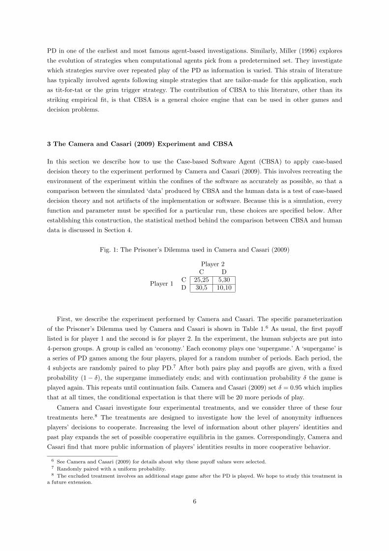
Fig. 1: The Prisoner’s Dilemma used in Camera and Casari (2009)
Player 2C D
Player 1C 25,25 5,30D 30,5 10,10
First, we describe the experiment performed by Camera and Casari. The specific parameterization
of the Prisoner’s Dilemma used by Camera and Casari is shown in Table 1.6 As usual, the first payoff
listed is for player 1 and the second is for player 2. In the experiment, the human subjects are put into
4-person groups. A group is called an ‘economy.’ Each economy plays one ‘supergame.’ A ‘supergame’ is
a series of PD games among the four players, played for a random number of periods. Each period, the
4 subjects are randomly paired to play PD.7 After both pairs play and payoffs are given, with a fixed
probability (1− δ), the supergame immediately ends; and with continuation probability δ the game is
played again. This repeats until continuation fails. Camera and Casari (2009) set δ = 0.95 which implies
that at all times, the conditional expectation is that there will be 20 more periods of play.
Camera and Casari investigate four experimental treatments, and we consider three of these four
treatments here.8 The treatments are designed to investigate how the level of anonymity influences
players’ decisions to cooperate. Increasing the level of information about other players’ identities and
past play expands the set of possible cooperative equilibria in the games. Correspondingly, Camera and
Casari find that more public information of players’ identities results in more cooperative behavior.
6 See Camera and Casari (2009) for details about why these payoff values were selected.7 Randomly paired with a uniform probability.8 The excluded treatment involves an additional stage game after the PD is played. We hope to study this treatment in
a future extension.
6
Now we discuss the CBSA implementation of the Camera and Casari experiment. CBSA shares all
primitives with CBDT, so there is a set of problems, a set of actions, and a set of results. A single learning
experience, called a case, is a problem, action, and result triplet. In addition to these three primitives,
CBSA follows case-based decision theory in defining a utility function, a similarity function, and an
aspiration level, as well as an additional parameter: introduced here, CBSAs have an act randomization
probability α ∈ [0, 1]. Finally, CBSA requires the definition of a so-called problem-result map or PRM.
The PRM is the transition function of the environment. We define all these objects below.
The experience of the human subject is to repeatedly play the Prisoner’s Dilemma, so we wish to
consider one round of play as generating one learning experience or case. Correspondingly, the set of
actions A is the set of actions in the one-shot Prisoner’s Dilemma: A = {C,D}, and the set of results Rare the payoffs found in Table 1: R = {5, 10, 25, 30}.
The set of problems is more complicated. The ‘problem’ can be thought of as the vector of information
observable by the player before the choice is made.9 In the Camera and Casari setting, the experimental
treatment is to vary the player’s observable information: therefore, the problem set definition varies with
the treatment. We define the problem set that corresponds to each of experimental treatments below—
but first we reason that in all treatments, players are aware of how far into the supergame they are, so
all treatments’ problem vectors include the period of play t. The other elements of the problem vectors
vary by treatment.
Treatment 1 is private monitoring, which consists of anonymous subjects playing the supergame with
no information about the player they are paired against or the players in the rest of the economy. Since
no other information is available, P1 = T , with typical element p1 = (t), where t ∈ T = {1, 2, 3, . . .}.Treatment 2 is anonymous public monitoring, which gives information about the history of other
players, including the highlighted history of one’s current opponent. However, explicit identifiers are
not available. In this treatment, we reason that the relevant information is the average cooperation
rate of ones current opponent. So P2 = T × [0, 1], with typical element p2 = (t, a (θ′)). The dimension
corresponding to the interval [0, 1] is the average cooperation rate of the opponent, where θ′ is the identity
of the opponent, and where a (θ′) is the average cooperation rate of opponent θ′.
Treatment 3 is non-anonymous public monitoring, which consists of the information available in
Treatment 2 as well as a unique ID of their opponent. We represent this as a vector of three binary
variables (id1, id2, id3), where at any time exactly one id variable is 1 and the others are 0. Therefore
P3 = T × [0, 1] × {0, 1} × {0, 1} × {0, 1}, with typical element p3 = (t, a (θ′) , id (θ′)), where θ′ is the
identity of the opponent, where a (θ′) is the average cooperation rate of opponent θ′, and where id (θ′)
is a string of dummy variables that indicate the identity of opponent θ′.
A tangent about the choice of Camera and Casari for testing CBSA: The fact that the experimental
treatment is to vary the information available to the players means that this setting is ideal for testing
CBSA, and is, in fact, one of the key factors we considered in selecting this experiment to model and
test. Since the treatments in the experiment imply different definitions of the set of problems P, this
experiment provides a set of a priori hypotheses that are empirically testable: that under the varying
definitions of the set P defined by the treatments, CBSA’s level of cooperation will move in tandem with
humans. Defining the problem sets requires some interpretation; that is, the treatments do not uniquely
identify corresponding problem sets. But, importantly, these problem set definitions were chosen without
regard for goodness-of-fit (they were chosen before statistical analysis).
9 This is akin to the player’s information set, but there is an important difference: the information set usually includesthe history of play. That is not necessarily the case here, because ‘history’ is typically handled by the player’s memory,that is, set of past learning experiences, and not the problem vector.
7
We assume the utility function u : R → R is simply the risk-neutral u(x) = x; this means that we
assume the payoffs of the game represent utility payoffs.
The similarity function s : P × P → [0, 1] describes how similar two circumstances are in the mind
of the CBSA. Pape and Kurtz (2013) found that, consistent with the evidence from psychology (Shep-
ard, 1987), that the similarity function has the following form, which was provided with an axiomatic
foundation by Billot, Gilboa, and Schmeidler (2008). We assume this functional form here:
s(p, q) =1
ed(p,q)
where p, q ∈ P
and d(p, q) =
√√√√# Dims∑i=1
[(pi − qi)2
]and pi refers to the ith element of p
The term “# Dims” refers to the number of dimensions of the problem set P: # Dims (P1) = 1,
# Dims (P2) = 2, and # Dims (P3) = 5. It is plausible that different dimensions could have differ-
ing weights, that could plausibly vary over time. These are called ‘attentional weights’ in the psychology
literature. We find these weights to be of little qualitative importance here so we do not consider them
explicitly.
There is an aspiration level H ∈ R, which represents a target level of utility of the agent. We explicitly
consider this as a fitted parameter.
Along with the decision primitives, CBSA defines the decision environment: i.e. those parts of the
choice problem that are external to the agent.10 In CBSA the decision environment is represented by
a function (algorithm) called the problem-result map or PRM. The PRM is the transition function of
the environment. It takes as input the current problem p ∈ P the agent is facing, the action a ∈ A that
the agent has chosen, and some vector θ ∈ Θ of environmental characteristics. The PRM returns the
outcome of these three inputs: namely, it returns a result r ∈ R; the next problem p′ ∈ P that the agent
faces; and a potentially modified vector of environmental characteristics θ′ ∈ Θ. I.e.:
PRM : P ×A×Θ → R×P ×Θ
In general in CBSA, θ describes the current state of the environment of each agent, i.e. exogenous,
unknown forces that are acting on the agent.11 In the setting of Camera and Casari, the environment
of the player is the identity of the opponent. Given this definition, the PRM finds the action a(θ)
chosen by the opponent, then (1) assigns the payoff associated with actions (a, a(θ)) to the result r, (2)
chooses a new opponent θ′, and (3) delivers the new problem vector p′ associated with opponent θ′. For
completeness, the explicit PRM is provided in Figure 7 (see Appendix B).
Figure 2 describes the choice algorithm which implements the core of CBSA, where the choice C
represents Cooperation and D represents Defect. It is an algorithmic description of the choice process
defined by CBDT, with two modifications. The modifications allow for imperfect memory. In Pape and
Kurtz (2013), it was found that a match between CBSA and human data was only achieved by allowing for
imperfect memory: otherwise CBSA solves the classification learning problem much faster than humans.
We find that imperfect memory is also important for matching human data in this setting.
10 These need not be defined for a decision theory, so are not a formal part of CBDT, and need only be formally definedwhen one seeks to generate simulated choice behavior to compare to empirical data.11 Known exogenous forces acting on the agent are part of the problem vector.
8

Fig. 2: The Choice Algorithm
Input: problem p, memory M.
1. For each a ∈ A:
(a) For each (q, a, r) ∈M, draw r.v. b(q,a,r) =
{1, with probability precall
0 otherwise.
Construct Ma ={
(q, a, r)∣∣b(q,a,r) = 1, AND
∃q ∈ P, r ∈ R s.t. (q, a, r) ∈M}
(b) Let Ua =
{∑(q,a,r)∈Ma
s(p, q)[u(r)−H
], if Ma 6= ∅
0, otherwise
2. Construct set BEST ={a ∈ A
∣∣Ua = maxb∈A {Ub}}
3. If #(BEST ) = 1 then let a? be the sole entry in BEST.If #(BEST ) = 2, then C is chosen with probability α, D with probability(1− α).
Output: Selected action a?
There are two kinds of imperfect memory. First, there is imperfect recall, governed by a probability
precall ∈ [0, 1]. Imperfect recall corresponds to an inability to access all memory at any given time, and it
is therefore associated with limited cognitive capacity. Second, there is imperfect storage, governed by a
probability pstore ∈ [0, 1]. Imperfect storage corresponds to a failure to add some experiences to memory
after they are experienced, and it is therefore associated with limited memory storage capacity.
In Figure 2, the agent faces a problem p ∈ P and has a memoryM⊆ C. In Step 1a, for each action a,
she collects those cases in which she performed this act. Since her recall is imperfect, relevant cases are
selected into the set Ma with probability precall, where relevant cases which are not recalled are simply
ignored.12 In Step 1b, she uses this subset of her memory Ma to construct a utility forecast of that act,
called here Ua. The agent then chooses the action which corresponds to the maximum U. As seen in step
3, when there is a tie between C and D, C is chosen with an exogenous probability α. In the original
formulation, it was assumed that α = .5, but in this study we calibrate α to data (see Section 4 for
calibration details).
Fig. 3: A Single Choice Problem.
Input: problem p, memory M, characteristics θ.
1. Input p, M into choice algorithm (Figure 2). Receive output a?.
2. Let (r, p′, θ′) = PRM(p, a?, θ).
3. With probability pstore,Let M’ =M∪ {(p, a?, r)}Else let M’ =M
Output: problem p′, memory M′, characteristics θ′.
Figure 3 describes a single choice problem faced by the agent. It embeds a reference to the choice
algorithm described in Figure 2. Figure 3 embeds the agent in an environment and explicitly references
12 When precall = 1, the agent has perfect recall. It then corresponds to CBDT as it appears in Gilboa and Schmeidler(1995).
9
that environment in the call to PRM. (The PRM corresponding to Camera and Casari’s experiment
is described above and also appears in Appendix B.) In Step One of the single choice prolem the agent
selects an act, a?. In Step Two, the action is performed in the sense that the environment of the agent
reacts to the agent’s choice: the PRM takes the current problem p, the action a? selected by the agent,
and the characteristics unobserved by the agent θ, and constructs a result r, a next problem p′, and a
next set of characteristics θ′. In Step Three, the agent’s memory is augmented by the new case which
was just encountered, so long as the agent does not have a ‘write-to-memory error:’ i.e., with probability
pstore, the case that was just experienced is added to the set M. With probability (1− pstore), that case
is discarded.
Since the choice problem depicted in Figure 3 maps a problem, a characteristic, and a memory vector
to another vector in the same space, it can be applied iteratively. A series of such iterations, along
with initial conditions and ending conditions, can then be used to produce a single time series of agent
behavior, called a ‘run.’ The ending condition used by Camera and Casari, as mentioned above, is a δ
probability of ending the supergame after each period. We follow this ending condition in the sense that
we simulate the actual lengths of play that appear in the data; see Section 4 below for details.
4 Statistical Model and Fitting Human Data
In this section, we describe the statistical and simulation method by which we estimate the parameters
of this model. First, we give an overview of the criteria we use to evaluate the explanatory power of the
parameterized model and the process we use to estimate those parameters, which includes a description
of the simulated data generation, the method we use to bootstrap standard errors for our parameters,
and a description of these free and constrained parameters. Then we discuss the relevant psychometric
literature, which is the source of this modeling perspective.
There are three criteria we use to evaluate the explanatory power of a model: qualitative fit, quanti-
tative fit, and model complexity.
Qualitative fit is equivalent to matching “stylized facts” of human data. For example, we find that,
empirically, Treatment 3 maintains a higher cooperation rate than Treatments 1 and 2 in all periods. A
model which matches more of these regularities is said to have a greater qualitative fit.
Quantitative fit is a numeric evaluation of fit to human data: for any given set of simulated data, we
construct Mean Squared Error (MSE) between the simulation average cooperation rate over time and
human average cooperation rate over time. The lower the MSE, the better the quantitative fit. Even
though perfect quantitative fit implies perfect qualitative fit, in practice quantitative fit can come at the
cost of qualitative fit. In the selection of best-fitting parameter values, we search the parameter space to
maximize quantitative fit and then evaluate qualitative fit of the best-quantitative-fit model.
Model complexity is known as ‘over-fitting’ in econometrics or ‘model elegance’ in theory. This third
criterion rests on the observation that if a model is allowed to be arbitrarily complicated, then perfect
qualitative and quantitative fit can be achieved, but such a model may be undesirable because it doesn’t
reveal insight into the phenomenon and is not generalizable out-of-sample. This consideration leads us
to select a simpler model over a more complicated one.13 Like qualitative fit, model complexity is an
ex-post evaluation criterion.
13 For another point of view on this criterion, consider two competing theories that attempt to explain the same phe-nomenon: theory a and theory b. Suppose that there is some empirical data available about the phenomenon. Supposetheory a has many more free parameters than theory b does. Now suppose we calibrate theories a and b to the data, and wefind, after calibration, that theory a and theory b both explain the same fraction of the variation in the data and explainthe same qualitative phenomena. Then, under the model complexity criterion, theory b is preferred.
10
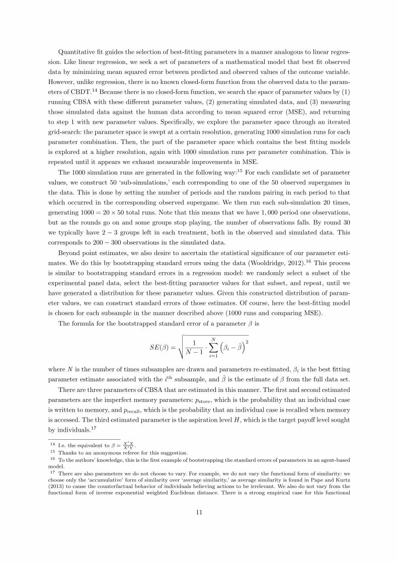
Quantitative fit guides the selection of best-fitting parameters in a manner analogous to linear regres-
sion. Like linear regression, we seek a set of parameters of a mathematical model that best fit observed
data by minimizing mean squared error between predicted and observed values of the outcome variable.
However, unlike regression, there is no known closed-form function from the observed data to the param-
eters of CBDT.14 Because there is no closed-form function, we search the space of parameter values by (1)
running CBSA with these different parameter values, (2) generating simulated data, and (3) measuring
those simulated data against the human data according to mean squared error (MSE), and returning
to step 1 with new parameter values. Specifically, we explore the parameter space through an iterated
grid-search: the parameter space is swept at a certain resolution, generating 1000 simulation runs for each
parameter combination. Then, the part of the parameter space which contains the best fitting models
is explored at a higher resolution, again with 1000 simulation runs per parameter combination. This is
repeated until it appears we exhaust measurable improvements in MSE.
The 1000 simulation runs are generated in the following way:15 For each candidate set of parameter
values, we construct 50 ‘sub-simulations,’ each corresponding to one of the 50 observed supergames in
the data. This is done by setting the number of periods and the random pairing in each period to that
which occurred in the corresponding observed supergame. We then run each sub-simulation 20 times,
generating 1000 = 20× 50 total runs. Note that this means that we have 1, 000 period one observations,
but as the rounds go on and some groups stop playing, the number of observations falls. By round 30
we typically have 2 − 3 groups left in each treatment, both in the observed and simulated data. This
corresponds to 200− 300 observations in the simulated data.
Beyond point estimates, we also desire to ascertain the statistical significance of our parameter esti-
mates. We do this by bootstrapping standard errors using the data (Wooldridge, 2012).16 This process
is similar to bootstrapping standard errors in a regression model: we randomly select a subset of the
experimental panel data, select the best-fitting parameter values for that subset, and repeat, until we
have generated a distribution for these parameter values. Given this constructed distribution of param-
eter values, we can construct standard errors of those estimates. Of course, here the best-fitting model
is chosen for each subsample in the manner described above (1000 runs and comparing MSE).
The formula for the bootstrapped standard error of a parameter β is
SE(β) =
√√√√ 1
N − 1·N∑i=1
(βi − β
)2where N is the number of times subsamples are drawn and parameters re-estimated, βi is the best fitting
parameter estimate associated with the ith subsample, and β is the estimate of β from the full data set.
There are three parameters of CBSA that are estimated in this manner. The first and second estimated
parameters are the imperfect memory parameters: pstore, which is the probability that an individual case
is written to memory, and precall, which is the probability that an individual case is recalled when memory
is accessed. The third estimated parameter is the aspiration level H, which is the target payoff level sought
by individuals.17
14 I.e. the equivalent to β = X′XX′Y .
15 Thanks to an anonymous referee for this suggestion.16 To the authors’ knowledge, this is the first example of bootstrapping the standard errors of parameters in an agent-based
model.17 There are also parameters we do not choose to vary. For example, we do not vary the functional form of similarity: we
choose only the ‘accumulative’ form of similarity over ‘average similarity,’ as average similarity is found in Pape and Kurtz(2013) to cause the counterfactual behavior of individuals believing actions to be irrelevant. We also do not vary from thefunctional form of inverse exponential weighted Euclidean distance. There is a strong empirical case for this functional
11

In addition to the three estimated parameters, there are two that are chosen according to theory. The
first parameter chosen in this way is the problem vector p, which was described above. The second is α,
the probability of cooperating when indifferent. A brief theoretical analysis proves that α will be equal
to the population average cooperation level in the first round of play. The logic is: at the beginning of
the supergame, all agents are indifferent between C and D and therefore randomize with probability α.
Therefore, a priori the first round of play will, on average, yield a fraction α of cooperators, which of
course turns out to be true in the simulated data.18
This method (other than bootstrapping) was used in the economic literature in Pape and Kurtz
(2013). In that paper, the authors use CBSA to evaluate CBDT’s ability to explain human learning be-
havior in a set of concept learning experiments from psychology, using psychological statistical methods
(‘psychometrics’). In this literature, mechanistic or algorithmic models of human behavior are used to
simulate data, which are compared to human behavioral data collected in the laboratory. They and we
follow the method used in the work of Nosofsky, Gluck, Palmeri, McKinley, and Glauthier (1994), which
advanced the statistics of this field; in their own words, “although previous researchers have discussed
the ability of different models to account for qualitative aspects of [concept learning experimental] data,
in this research we begin the process of quantitatively testing such models (Nosofsky et al, 1994, p. 354).”
Like us, Nosofsky et al search the space of free parameters to minimize the sum of square deviations
between the (average) predicted and (average) observed outcome variable.19 This method is widely ac-
cepted in psychology, which uses these kinds of models fitted to ‘micro-level’ experimental panel data
using algorithmic models like ours.20 This method also bears some similarity to calibration of macroeco-
nomic models (Kydland and Prescott, 1996): perhaps the most important difference between this method
and macroeconomic model calibration is that macroeconomic models calibrate to time-series instead of
panel data. We intend to investigate this relationship more thoroughly in future work.
A final comment on this method: matching the simulated average data to the average of the outcome
variable of the data ignores variance of those data. It stands to reason that it may be valuable to count
more heavily observed outcomes that have low variance in data. Here we are also able to follow Nosofsky
et al (1994), who present a weighted mean squared error, where the weights are chosen to address this
concern: “The weighted [mean squared error] is found by [averaging] the squared deviation between
the predicted and observed error proportions weighted by 1σ2 , the inverse of the variance of each cell
proportion[.] (Nosofsky et al, 1994, p. 362)”21 We try estimation with weighted mean squared error, and,
like Nosofsky et al, find it has little effect on the results. Therefore, we do not present these results here.
5 Experimental Results
In this section we present the results of two versions of CBSA and compare them to the results of
the Probit found in Camera and Casari (2009) and a constrained alternative Probit formulation. The
purpose of this comparison is to validate CBSA: we seek to empirically ‘benchmark’ CBSA against some
form in psychology, which is bolstered by the results found in Pape and Kurtz (2013). Please see that paper and Section 3of this paper for details.18 An alternative modeling choice is to posit a two types of agents: ones who always cooperate when indifferent and ones
who always defect. Then one calibrates the relative size of the two populations to the known cooperation rate in the firstround. This alternative modeling strategy does not make a large difference in the results so it is not presented here.19 In the case of concept learning the outcome variable in question is the rate of misclassification of particular objects
over time in a supervised learning environment.20 E.g. Nosofsky and Palmeri (1996), Love, Medin, and Gureckis (2004), Kurtz (2007), and Vigo (2013).21 They cite Bishop et al (1975) as a statistical source for this method.
12

alternative explanatory model. We compare the four models by the model selection criteria described in
the previous section: quantitative fit, qualitative fit, and model complexity. An overview of the results can
be seen in Table 1. In this table, we provide parameter estimates for the two CBSA versions and degrees of
freedom and goodness-of-fit (MSE) of all four available models. The predicted outcome variable, average
cooperation rates over time, for all four models as well as the raw data are shown in Figure 4. We also
organize these predicted outcome variables by treatment and include 95% confidence intervals (the gray
area around the CBSA prediction) in Figure 5.
We are able to show (1) that the CBSA correctly predicts the empirically observed trajectory of
average cooperation rates over time across different treatments, and (2) that the choice behavior implied
by CBSA is a closer fit to the empirical data than either Probit model. We also find that the best-fitting
parameters suggest (3) humans aspire to payoff value above the mutual defection outcome but below
the mutual cooperation outcome, which suggests they hope but are not confident that cooperation can
be achieved, and (4) circumstances with more details are easier to recall. We also predict that, if the
experiments of Camera and Casari were run for more periods, that we would begin to see an increase in
cooperation among the players.
Probit and CBSA methods with similar goals: the coefficient estimates of a Probit emerge from an
analytical maximization of a likelihood function given the data, and the CBSA parameter estimates
emerge from a computational maximization of a quantitative measure of fit to data. In this sense, they
are both predictive methods calibrated to data. Therefore, one could think that, if CBSA compares
favorably to the Probit along some goodness-of-fit metric, then perhaps CBSA should be considered
more seriously as an empirical method. On the other hand, if CBSA compares unfavorably to the Probit,
it should be considered less seriously.
Note that this does not imply we seek to accept Probit over CBSA or the reverse. This is because
CBSA and Probit could both be true. Suppose both the Probit and CBSA were good fits to explain the
empirical data. One explanation could be that CBSA explains human learning behavior, and the memory,
similarity, and utility of CBSA together encode strategies that the Probit measures, even though CBSA
does not explicitly represent strategies.22 Another explanation notes that Decision Theory is built on
representation theorems: if behavior matches certain axioms, then a utility function, beliefs, etc., that
represent that choice can be constructed. However, in decision theory, no representation theorem claims
exclusivity: on the contrary, so long as the axiom sets of two representation theorems are not mutually
exclusive, then the choice behavior can be represented by the structures in each theorem. So if the
Probit and CBSA both seek to explain behavior in the ‘representation theorem’ sense, they could both
be valid.23,24
This section proceeds in four parts: First, we describe the four models depicted here. Second, we
compare the two CBSA models and the two Probit models along the dimensions of quantitative fit and
model complexity using Table 1. Third, we compare the four models along the dimension of qualitative
fit by using Figure 4. Steps two and three establish results (1) and (2) above, that CBSA fits well and
22 This is possible if one notes that these computational structures of CBSA could ‘encode strategies’ in the way that acomputer program encodes program behavior.23 Moreover, Matsui (2000) shows that Case-based Decision Theory and Expected Utility Theory can both represent the
same choice behavior almost always. If the Probit can be likened to an expected utility perspective, then Matsui’s resultwould suggest that both the Probit and CBSA could match.24 It is interesting to consider running the models on each others’ outcomes: what strategies does a Probit suggest that
the CBSA has encoded? And, in the other direction, what CBSA parameters emerge when CBSA seeks to predict theimplied Probit strategies? We intend to consider these questions in a future extension.
13
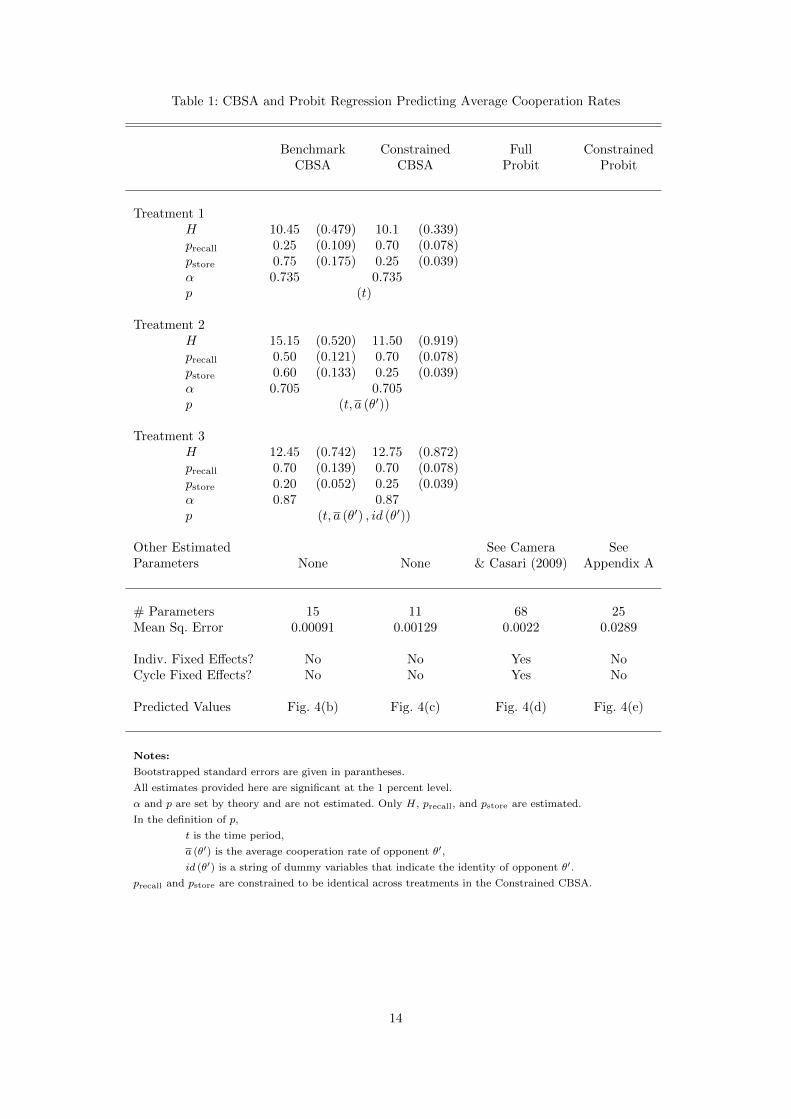
Table 1: CBSA and Probit Regression Predicting Average Cooperation Rates
Benchmark Constrained Full ConstrainedCBSA CBSA Probit Probit
Treatment 1H 10.45 (0.479) 10.1 (0.339)precall 0.25 (0.109) 0.70 (0.078)pstore 0.75 (0.175) 0.25 (0.039)α 0.735 0.735p (t)
Treatment 2H 15.15 (0.520) 11.50 (0.919)precall 0.50 (0.121) 0.70 (0.078)pstore 0.60 (0.133) 0.25 (0.039)α 0.705 0.705p (t, a (θ′))
Treatment 3H 12.45 (0.742) 12.75 (0.872)precall 0.70 (0.139) 0.70 (0.078)pstore 0.20 (0.052) 0.25 (0.039)α 0.87 0.87p (t, a (θ′) , id (θ′))
Other Estimated See Camera SeeParameters None None & Casari (2009) Appendix A
# Parameters 15 11 68 25Mean Sq. Error 0.00091 0.00129 0.0022 0.0289
Indiv. Fixed Effects? No No Yes NoCycle Fixed Effects? No No Yes No
Predicted Values Fig. 4(b) Fig. 4(c) Fig. 4(d) Fig. 4(e)
Notes:
Bootstrapped standard errors are given in parantheses.
All estimates provided here are significant at the 1 percent level.
α and p are set by theory and are not estimated. Only H, precall, and pstore are estimated.
In the definition of p,
t is the time period,
a (θ′) is the average cooperation rate of opponent θ′,
id (θ′) is a string of dummy variables that indicate the identity of opponent θ′.
precall and pstore are constrained to be identical across treatments in the Constrained CBSA.
14
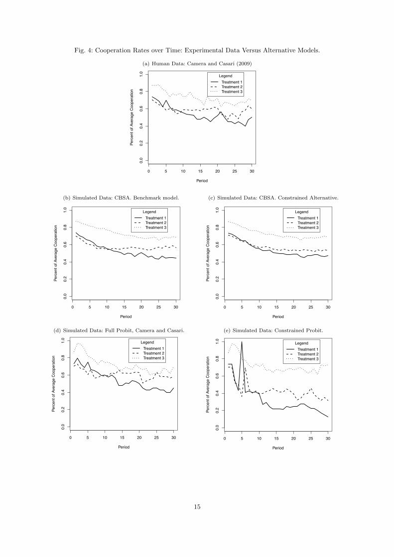
Fig. 4: Cooperation Rates over Time: Experimental Data Versus Alternative Models.
(a) Human Data: Camera and Casari (2009)
0 5 10 15 20 25 30
0.0
0.2
0.4
0.6
0.8
1.0
Period
Perc
ent o
f Ave
rage
Coo
pera
tion
Human−subject Experimental Results by Treatment
LegendTreatment 1Treatment 2Treatment 3
(b) Simulated Data: CBSA. Benchmark model.
0 5 10 15 20 25 30
0.0
0.2
0.4
0.6
0.8
1.0
Period
Perc
ent o
f Ave
rage
Coo
pera
tion
LegendTreatment 1Treatment 2Treatment 3
(c) Simulated Data: CBSA. Constrained Alternative.
0 5 10 15 20 25 30
0.0
0.2
0.4
0.6
0.8
1.0
Period
Perc
ent o
f Ave
rage
Coo
pera
tion
LegendTreatment 1Treatment 2Treatment 3
(d) Simulated Data: Full Probit, Camera and Casari.
0 5 10 15 20 25 30
0.0
0.2
0.4
0.6
0.8
1.0
Period
Perc
ent o
f Ave
rage
Coo
pera
tion
Full Probit Results by Treatment
LegendTreatment 1Treatment 2Treatment 3
(e) Simulated Data: Constrained Probit.
0 5 10 15 20 25 30
0.0
0.2
0.4
0.6
0.8
1.0
Period
Perc
ent o
f Ave
rage
Coo
pera
tion
Probit Results by Treatment
LegendTreatment 1Treatment 2Treatment 3
15
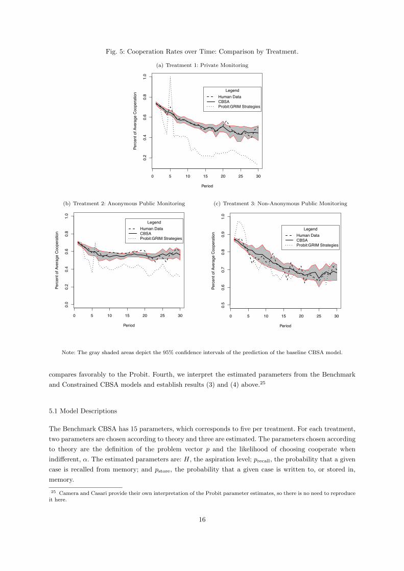
Fig. 5: Cooperation Rates over Time: Comparison by Treatment.
(a) Treatment 1: Private Monitoring
0 5 10 15 20 25 30
0.2
0.4
0.6
0.8
1.0
Period
Perc
ent o
f Ave
rage
Coo
pera
tion Legend
Human DataCBSAProbit:GRIM Strategies
(b) Treatment 2: Anonymous Public Monitoring
0 5 10 15 20 25 30
0.0
0.2
0.4
0.6
0.8
1.0
Period
Perc
ent o
f Ave
rage
Coo
pera
tion
LegendHuman DataCBSAProbit:GRIM Strategies
(c) Treatment 3: Non-Anonymous Public Monitoring
0 5 10 15 20 25 30
0.5
0.6
0.7
0.8
0.9
1.0
Period
Perc
ent o
f Ave
rage
Coo
pera
tion
LegendHuman DataCBSAProbit:GRIM Strategies
Note: The gray shaded areas depict the 95% confidence intervals of the prediction of the baseline CBSA model.
compares favorably to the Probit. Fourth, we interpret the estimated parameters from the Benchmark
and Constrained CBSA models and establish results (3) and (4) above.25
5.1 Model Descriptions
The Benchmark CBSA has 15 parameters, which corresponds to five per treatment. For each treatment,
two parameters are chosen according to theory and three are estimated. The parameters chosen according
to theory are the definition of the problem vector p and the likelihood of choosing cooperate when
indifferent, α. The estimated parameters are: H, the aspiration level; precall, the probability that a given
case is recalled from memory; and pstore, the probability that a given case is written to, or stored in,
memory.
25 Camera and Casari provide their own interpretation of the Probit parameter estimates, so there is no need to reproduceit here.
16

The Constrained CBSA is an alternative specification of CBSA. It comes from the following obser-
vation: given the fact that data were provided to the subjects of the experiment in all treatments in an
identical way, perhaps memory is written to and accessed in an identical away across treatments. The
Constrained CBSA formalizes this hypothesis by constraining that the probability of recall precall and
the probability of storage pstore to be the same across all three treatments. (The aspiration level H, the
initial rate of cooperation α, and the definitions of the problem vector vary across treatments.) As a
consequence, the Constrained CBSA has 11 parameters total, only 5 of which are estimated.
The Full Probit refers to the Probit analysis which appears in Camera and Casari (2009), Table 4,
page 994. Camera and Casari propose three strategies players might use, and their Probit attempts to
empirically identify the relative importance of these strategies in determining behavior. The three strate-
gies are: reactive strategies, global strategies, and targeted strategies. Reactive strategies are: choosing
to defect after one’s opponent defects. Global strategies are: choosing to defect when any player in the
economy defects. Targeted strategies are: choosing to defect against players who have defected against
oneself, but ignoring defections against others. Each of these strategies is associated with a lag of one
to five periods after a subject experiences a defection, so that the marginal response from a defection
can change over those five periods. Camera and Casari’s Probit regression is designed to identify the
marginal effects of these different strategies, where the binary outcome variable is the choice to cooperate
and observations are people-periods. The probit also includes individual and cycle fixed effects, for a total
of 68 estimated parameters.
We created the Constrained Probit as a variant to the Camera and Casari Probit. It is the same as the
Full Probit, except that there are no cycle and individual fixed effects. The reason for the Constrained
Probit is to make a fair comparison to CBSA along the following dimension: because CBSA does not fit
parameters for different cycles and individual subjects, it can predict out-of-sample in its current form.
However, the Full Probit allows independent fitting for individuals. These individual fixed effects would
not be available for predicting out-of-sample. So the Constrained Probit is, in some sense, the best-fitting
Probit which allows for the same freedom to predict out of sample as does CBSA. (The same reasoning
could be applied to out-of-sample prediction for any econometric model. It guards against over-fitting.)
The Constrained Probit has 25 estimated parameters. The results of the Constrained Probit can be found
in the Appendix A.
For all four models–the two CBSAs and the two Probits–we construct the aggregate level of cooper-
ation in each time period t:
CLt =∑i∈It
ai,tNt
Where It is the set of subjects still playing at time t, Nt is the number of subjects still playing at time t,
and where ai,t equals 1 if a player i chooses Cooperate and 0 if she chooses Defect. In the experiment, Nt
varies with treatment and time period. In the CBSA results, Nt is as high as 4, 000 (we simulate 1, 000
economies, each with four players, and as supergames end in the data, this value falls). To generate CLt
in the Full and Constrained Probit, we use the predicted value of the dependent variable, Yi, for each
agent in the data. Yi is the probability of cooperating. We record a binary value of 1 if Yi ≥ 0.50 and
0 if Yi < 0.50. Then we construct the average cooperation level of all observations per period across
economies as described above.
17

5.2 Model Comparison: Quantitative Fit and Model Complexity (Results 1 and 2)
Table 1 summarizes both the quantitative fit, MSE, and one measure of model complexity, the number
of estimated parameters. It also depicts the bootstrapped standard errors.
With regard to quantitative fit, the order of Mean Squared Error (MSE) is:
Benchmark CBSA < Constrained CBSA ≤ Full Probit << Constrained Probit
The Benchmark CBSA is a better fit than any other model available by a significant degree. The next best
is fit the Constrained CBSA, although the Full Probit is close (only 22% larger MSE). The Constrained
Probit performs far worse than the others: its MSE is over 30 times that of the Benchmark CBSA and
ten times that of the Full Probit.
These results are particularly striking when one considers the model complexity. The Full Probit is
worse at explaining the average cooperation rates despite having four times the number of free parameters.
The Full Probit, as opposed to the Constrained Probit, also takes advantage of individual fixed effects,
which CBSA does not allow (CBSA assumes that all agents are ex-ante identical and differ only because
of experiences over the course of the run.) Dropping individual fixed effects in the Constrained Probit
reduces the model complexity to only about twice that of the Benchmark CBSA, but at the cost of large
amounts of predictive power.
5.3 Model Comparison: Qualitative Fit (Results 1 and 2)
Figure 4 visually depicts the actual average cooperation rates in the experiment versus the four models’
predicted average cooperation rates. Figure 4(a) depicts the average cooperation rates over time in
the human trials as found by Camera and Casari. Figures 4(b) and 4(c) depict the average predicted
cooperation rates over time in the CBSA models; first the Benchmark, then the Constrained. Figures 4(d)
and 4(e) depict the predicted average cooperation rates over time which arise from the Probit models;
first the Full, then the Constrained.
Consider the following observations about the human cooperation rates as seen in Figure 4(a). First,
Treatment 3 does not overlap with Treatments 1 and 2 and instead lies strictly above it for the entirety
of the thirty periods. Second, Treatment 1 involves somewhat more cooperation than Treatment 2 in
early periods, until some time between rounds 5 and 10, where Treatment 2 begins to involve more
cooperation. Treatment 2 continues to involve more cooperation until the end, with the exception of
a brief time around Period 20. Third, average cooperation rates appear to settle into their long-run
averages around period fifteen or so. There is a possible upward drift in the three treatments, suggesting
if the experiments were to have gone on longer, perhaps average cooperation rates would be u-shaped.26
The CBSA predicted cooperation rates, Figures 4(b) and 4(c), match the human data qualitatively
quite well. First, Treatment 3 is strictly above the other treatments for the entirety of the run. Second,
Treatment 1 has an early lead in cooperation over Treatment 2, but switches places around between
periods 5 and 10, as in the human data. (It also ignores the brief reversal around Period 20, which looks
like noise.) The crossover occurs a bit too early in the Constrained CBSA. Third, average cooperation
rates settle into their long run averages fairly early, although apparently earlier than the human data
(more likely by Period 10 to 15). There is also a possible upward drift in all treatments near the end, par-
26 This is also predicted in the long run by CBSA; see Section 5.4 below.
18
ticularly in Treatment 2. The upward drift in Treatment 2 is perhaps too pronounced in the Constrained
CBSA.
The Full Probit, Figure 4(d), matches the human data somewhat well: Treatment 3 is largely above
the other two treatments, Treatment 1 and 2 switch as they do in the human data, with overlap seen in
the human data. Also, there appears to be some possible upward drift in all Treatments near the end.
The most significant way that the Full Probit matches the human data better than the CBSA data is,
Treatment 1’s spike around period 5. The Full Probit has this spike (and the Constrained Probit has it in
an even more exaggerated way). CBSA has this spike only mildly (and, in fact, CBSA seems significantly
less noisy than the Probit). In the authors’ opinion, this brief spike is likely just noise in the human data
and not a meaningful feature to attempt to match. So the extent to which the Full Probit ‘overfits’ on
such features, it would suggest that CBSA is a better qualitative fit. On the other hand, if one believes
that the period 5 spike in the human data is not noise, that the Full Probit picked it up is to its favor.
This spike does cause the Constrained Probit to violate the ordering that Treatment 3 has higher
cooperation rates than Treatments 1 and 2 over the whole trial. Although the Full Probit matches the
trajectory and final average cooperation rates fairly well, under the Constrained Probit, the average
cooperation rates for the Probit under Treatments 1 and 2 falls much faster than either the human data
or the benchmark CBSA, resulting in a final average level of cooperation much lower than the observed
level of cooperation. Finally, in Treatments 1 and 2, there is definitely no upward drift seen, although
possibly in Treatment 3.
Also consider Figure 5, in which, using the bootstrap method we calculate the standard errors of the
predicted cooperation rate for the CBSA benchmark model and display the 95% percent level confidence
intervals, shown as the gray area around the CBSA prediction. This provides us with the measure of
variation in prediction which appears to fit the experimental data quite well in all three treatments. This
provides further qualitative evidence that CBSA can consistently predict the average cooperation rates
in the empirical data over time.
5.4 CBSA: Interpretation of Estimated Parameters (Results 3 and 4)
We can establish, using bootstrapped standard errors, that all of the point estimates in the CBSA models
are highly significant at the 1 percent level. Furthermore, the individual estimates from the treatments
are different from each other in most cases. There are significant differences between the estimates in the
benchmark CBSA of H between treatments at the 5 percent level, found by using Z-test. The estimates
of pstore are not statistically different from each other at the 10 percent level across almost all treatments.
The precall is statistically different when comparing treatment 3 to the other treatments. The estimates
of precall and pstore do not have a consistent ordering.
Here we interpret the values of the estimated parameters, precall, pstore, and H, in the best-fitting
CBSA models and establish the results three and four: (3) that the aspiration levels are ‘reasonable’ and
(4) the memory parameters circumstances with more details are easier to recall.27 In the course of the
presentation we investigate these claims with the aid of some robustness tests.
Result 3: The aspiration level H represents a target payoff level that the agent seeks in the PD Stage
game (Table 1). For the Benchmark and Constrained CBSAs, the fitted values for all three treatments
are above the (D,D) payoff (10) but below the (C,C) payoff (25). This suggests that agents hope to
27 We do not interpret p, the problem set, and α, the probability of cooperating when indifferent, because they are setby theory; therefore, their values are not a “finding” and are therefore it is not appropriate to interpret them as one wouldestimated parameters. Please see Section 3 for how those parameters were chosen.
19

do better than the stage game Nash equilibrium but are not confident that they will. Aspiration levels
can also be interpreted as the satisficing payment required for a subject to stop searching for a better
outcome. This leads to an interpretation of the aspiration level as a weighted average of the two symmetric
outcomes, (C,C) and (D,D).28 In the benchmark model, this interpretation implies that the agent only
hopes for the mutual co-operation outcome about 3% of the time in Treatment 1, 34% of the time in
Treatment 2, and 16% of the time in Treatment 3. (The values are similar in the Constrained CBSA.)
The aspiration level is higher in 2 than in 1, and higher in 3 than in 1. This is consistent with the
interpretation that agents hope more monitoring will increase cooperation. However, that interpretation
is somewhat undercut by the fact that the aspiration level is higher in Treatment 2 than in Treatment 3.
We run a robustness test by varying the aspiration level to examine the implications of behavior in
our model. In the Benchmark CBSA, when the aspiration level H is set to be higher than achievable,
31, the mean squared error increases about twenty eight-fold, to 0.022. When it is constrained to be
below the worst payoff, 4, the MSE increases about twenty five-fold, to 0.025. The fact that reasonable
aspiration values provide a better fit than ‘unreasonable’ aspiration values should be interpreted as a
vote in favor of CBSA being the correct model specification.
It is worth considering the behavior one expects with different aspiration levels. As mentioned in the
description of CBDT, aspiration levels function as a satisficing level. This can be seen in the functional
form of case-based utility, which awards a payoff of [u(r) − H] for a case in memory which yields an
outcome r. Consider a new experienced case (p, a, r). If u(r) falls short of H, this new case would tend
to discourage action a in circumstance p (or other, similar circumstances), while if u(r) exceeds H, this
case encourages this same action in such circumstances.29
This implies that aspiration levels have the following behavioral implications: a very low aspiration
level yields quick ‘convergence’ in behavior for all circumstances that is heavily influenced by early choices.
A very high aspiration level yields continuous ‘searching,’ so agents are seen vacillating between defection
and cooperation for the same or similar circumstances. An intermediate aspiration level, then, leads to
some searching. For circumstances that are predictive of opponent’s behavior and therefore of the payoffs
associated with ones own actions, the agent may learn which action is appropriate (yields the highest
available payoff) and circumstances that are not predictive (or predictive of only low-payoff-outcomes)
will prompt the agent to continue to search.
Result 4: The memory probabilities precall and pstore can be interpreted as follows: A low precall
implies the relevant limitation is cognitive capacity, while a low pstore implies that the relevant limitation
is memory space. These parameters vary across the three treatments in the Benchmark CBSA, and are
constrained to be identical in the Constrained CBSA.
Let us consider the ordering of precall across treatments in the Benchmark CBSA. In recall probability
precall, this is the ordering: precall(Treat1) < precall(Treat2) < precall(Treat3). This suggests as the length
of the problem vector (i.e. available information) increases, the probability of recall increases. This seems
counter-intuitive: the longer the problem vector, the more information must be recalled in the future.
Presumably more information is more difficult to store and recall than less information, which would
make it harder, not easier, to recall. On the other hand, adding information that is relevant to the
problem could have the opposite effect. For example, if one has access to the opponent’s ID, it may
take less effort to store and recall cases from earlier periods because there is a ‘marker’ to attach those
28 One could also interpret the value as being induced by some ‘hope distribution’ over all four payoff values, 5, 10, 25,and 30.29 The agent-based modeling literature describes these two behaviors as ‘exploration’ versus ‘exploitation,’ so aspiration
levels determine the switch from exploration to exploitation.
20
memories to: this ID variable. In any case, the apparent empirical fact is that the recall probability is
inversely related to the length of the problem vector.
Although in previous work (Pape and Kurtz, 2013), it was found that precall was found to be smaller
than pstore, that does not to hold in this experiment, where we find that Treatment 1 and 2 have precall
less than pstore, but Treatment 3 and the constrained CBSA have the reverse.
For storage probability pstore, the ordering suggests that the probability of storage decreases the length
of the problem vector: pstore(Treat3) ≤ pstore(Treat2) < pstore(Treat1). However, this set of orderings is
not statistically significant at the 10% level.
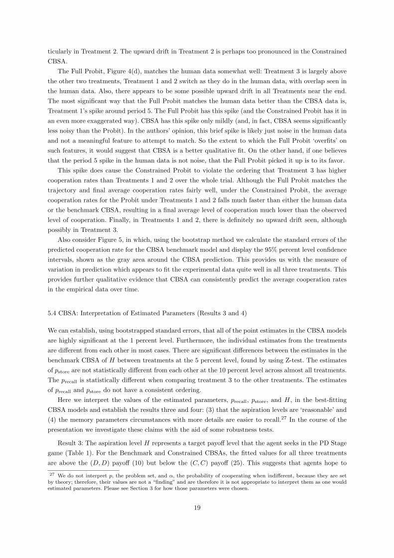
Fig. 6: Cooperation Rates: Benchmark in the Long Run versus Perfect Memory
(a) Perfect Memory
0 5 10 15 20 25 30
0.0
0.2
0.4
0.6
0.8
1.0
Period
Perc
ent o
f Ave
rage
Coo
pera
tion
LegendTreatment 1Treatment 2Treatment 3
(b) Benchmark Model in Long Run
0 50 100 150 200
0.0
0.2
0.4
0.6
0.8
1.0
Period
Perc
ent o
f Ave
rage
Coo
pera
tion
LegendTreatment 1Treatment 2Treatment 3
Next we consider the implications of perfect memory in the CBSA. When we only consider perfect
memory, i.e. precall = pstore = 1, we find that the MSE worsens significantly. When memory is constrained
to be perfect, the MSE increases about one hundred-fold, to 0.10. This suggests that imperfect memory
may be more important than reasonable aspiration values. In Figure 6(a), we see that in Treatments 1
and 2, the downward trend quickly reverses toward perfect cooperation, and even Treatment 3 shows
some upward drift near the end of the displayed timeframe. (The other parameter values are kept at the
level set in Table 1). We compare these results to long run results of the benchmark model in Figure 6(b).
In this figure, the benchmark model is run for 200 periods. We see that even under imperfect memory,
cooperation heads toward perfect cooperation in Treatment 2, with some upward tendency in Treatment
3 as well. We also find that for an increase in memory over those values found in Table 1 (not shown here),
Treatments 1 and 3 also head toward perfect cooperation in this timeframe. This pattern is robust to
lowering the probability of cooperation when indifferent, so this is not a product of over-selection under
indifference. Instead, what is happening is that agents eventually ‘find’ the cooperative outcome and
then, as they go into the future, the early events that led to defection fade into the past and cooperation
wins over. When there is perfect memory, this effect occurs too early to be consistent with the human
data.
This observed effect makes an out-of-sample prediction: we predict that among human players, if
game play was allowed to continue we would expect that the leveling off would eventually turn around
21
to increasing cooperation in the long run, most strongly with Treatment 2. This suggests it would be
valuable to do repeated Prisoner’s Dilemma experiments for longer time spans (i.e. higher continuation
probabilities) to see whether this out-of-sample prediction is achieved.
6 Discussion
In this section, we discuss the broader implications of these results. To the author’s knowledge, this is
the first application of case-based decision theory to a strategic/game-theoretic context. What is the
appropriateness of such an application? After all, case-based decision theory is developed for individual
choice; is it appropriate to view game play as merely another form of decision-making? And, given this
match in this strategic setting between case-based decision theory—as implemented through CBSA—
and human choice, what have we learned about case-based decision theory? What have we learned about
learning in games?
Let us consider strategic choice problem as a decision theory problem in the expected utility paradigm.
In order to do so, one must define the state space. The state space in this setting is the set of possible
strategies (complete contingent plans) that one’s opponent (and Nature) might use. From this per-
spective, the mapping of a game into the expected utility framework is straight-forward. Consider von
Neumann and Morgenstern in The Theory of Games and Economic Behavior : they transform an arbi-
trarily complicated finite game into a game in which each player makes one move which specifies all of
their contingent plays; each player submits this move to an umpire who then works out the payoffs for all
players. This results in a single expression for the player’s probability-weighted payoff, “his ‘mathemati-
cal expectation’ of the outcome (von Neumann and Morgenstern, 1944, Section 11.2.3).” They continue:
“The player’s judgement must be directed solely by this ‘mathematical expectation,’—because the var-
ious moves [of other players and Nature] are completely isolated from each other.” (The mathematical
expectation referred to here is expected utility as von Neumann and Morgenstern define it (See von
Neumann and Morgenstern, 1944, Section 5.2.2).) The only remaining issue to determine choice is the
probability distribution over other players’ strategies. The zero-sum analysis of von Neumann and Mor-
genstern and Nash’s subsequent work (Nash, 1950, 1953) can be thought of as a search of this space for
‘reasonable’ priors. This historical note justifies the approach of viewing strategic choice as another form
of individual choice. Furthermore, and in justification of case-based decision theory specifically, the fact
that the state-space representation is well-defined mathematically does not imply that it is intuitive for
actual human players. If it is not intuitive for actual human players, then the objection of the state-space
representation described by Gilboa and Schmeidler in their original work (Gilboa and Schmeidler, 1995):
if the state-space is not intuitive for agents, then it might not be how agents actually represent their
problem, so the conclusions of that theory may not be helpful in understanding how humans actually
choose. Saying the reverse, finding a representation that is more intuitive for people may lead to a theory
that is better at predicting how people actually choose.
Along those lines, consider the theoretical (vs. empirical/experimental) game theory literature of
learning in games. The basic problem faced by researchers in this literature is that for an agent to “learn”
the strategy of her opponent, one of two things must hold: she must have some a priori rule to extrapolate
from past actions to future actions or some a priori restriction on the set of possible strategies that are
allowable. Why? Nachbar (1997) makes a concise formal argument: “Formally, if a player can learn to
predict the continuation path of play then, in particular, the player can learn to predict the distribution
over play in the next period. Let a one-period-ahead prediction rule be a function that, for each history,
22
chooses a probability distribution over the opponent’s stage game actions. [...] [F]or any one-period-ahead
prediction rule, whether or not derived via Bayesian updating, there exists an opposing strategy that
does “the opposite.” [...] [S]o there is no one-period-ahead rule that is asymptotically accurate against all
strategies (Nachbar, 1997, p. 227, footnote 3.).” From this perspective, the learning-in-games literature
can be thought of as proposing different extrapolation rules and/or restricted subsets. Nachbar (1997),
for example, proposes a set of ‘conventional’ strategies, and supposes that (it is common knowledge
that) agents have a lexicographic preference for conventional vs. unconventional strategies. Another
prominent example is Fudenberg and Kreps (1993, 1995), who suppose that opponents’ play corresponds
to historical frequencies of past play (“fictitious play”) which leads to so-called self-confirming equilibria.
From this perspective, case-based decision theory is simply one such extrapolation rule. Why choose
a case-based rule? The first justification is, of course, the empirical success of Pape and Kurtz (2013)
explaining human learning in another setting. Another justification, however, relates directly to this basic
problem that Nachbar describes so effectively. In the early history of the philosophy of learning, Hume
(1748) introduced the ‘induction problem.’ Gilboa and Schmeidler take as some inspiration of case-based
reasoning Hume’s observation that “[f]rom causes which appear similar we expect similar effects. This is
the sum of all of our experimental conclusions (Hume, 1748).” The reference to similarity is the inspiration
of Gilboa and Schmeidler to formally incorporate ‘similarity’ in their model. Nachbar’s observation that
there must be some a priori extrapolation rule or a priori restriction on the set possible ideas in order
to learn from experience is essentially a restatement of the induction problem as introduced by Hume.
Now, Hume’s point is that, inferring from past events to future events falls short of ‘true knowledge’ as
one might want from a philosophical point of view; that is not the point here, however. The point here is
to take Hume’s claim as a hypothesis regarding human learning behavior: that actual people extrapolate
from past events to future events using similarity. This is a strong, historically-rooted justification for
using a case-based approach to model human behavior in learning-in-games. Moreover, since we find
that case-based decision theory provides a good match for human learning behavior, it suggests that the
development of a formal equilibrium concept along these lines—a case-based equilibrium—could be a
fruitful endeavor. Perhaps the most profitable direction would be to investigate the relationship between
learning implied by case-based decision theory and fictitious play proposed by Fudenberg and Kreps.30
One vein of experimental/empirical game theory literature regarding learning in games involves ex-
plaining human game-play using reinforcement learning (Roth and Erev, 1995b; Bereby-Meyer and Erev,
1998; Erev and Roth, 1998; Erev, Bereby-Meyer, and Roth, 1999; Erev and Roth, 2001). The Roth, Erev,
and Bereby-Meyer papers measure success in explaining human data by considering the mean squared
deviation between average results of simulated and observed data, as we do here. This supports the
methodology we describe in Section 4. In reinforcement learning, each agent keeps track of a weight
(value) for each action which indicates her proclivity to take that action. When she takes an action and
it delivers a payoff which exceeds some reference level, she increases the weight on that action, and when
it falls short, she decreases the weight on that action. Reinforcement learning can be made more complex:
for example, the reference level can vary over time and be endogenous to experience in some manner,
or the agent can have multiple sets of action weights, so that different circumstances invoke different
action weights. Reinforcement learning is related but distinct from case-based learning. For example, in
both theories, reference levels or aspiration levels play a key “sign-changing” role. The major difference
is: first of all, CBDT does not collapse history into a single set of weights, so CBDT allows for history to
be re-examined later in the agent’s experience. Also, CBDT has similarity, which seems to be a critical
30 We intend to develop this relationship in future work.
23
component to getting human learning behavior correct.31 Although we do not explicitly compare rein-
forcement learning vs. case-based decision theory on the Camera and Casari data, following the work of
Pape and Kurtz (2013), it can be shown that while ‘simple’ case-based learning reproduces the ordering
of difficulty of human concepts found in the psychological concept learning experiments of Nosofsky and
Palmeri (1996), reinforcement learning does not.32 Since differences between these approaches can be
found, it suggests that we may learn more about case-based learning by a closer comparison between
CBSA and reinforcement learning, which we intend to pursue in a future extension.
7 Conclusion
In this paper, we use Case-based Decision Theory to explain the average cooperation level over time of
the repeated Prisoner’s Dilemma among random pairs of people in a small group; the work of Camera
and Casari (2009). We are the first to use a method called the Case-based Software Agent and show that
CBSA (and therefore CBDT) empirically explains human behavior in a strategic, dynamic, multi-agent
setting. This provides a different frame of reference to view the results in the iterated prisoner’s dilemma
game that incorporates past experiences into explaining sustained cooperative outcomes.
We establish four main results.
First, we find that CBSA predicts human behavior in this strategic and dynamic setting quite well. It
has a good quantitative fit, and its predicted outcome variable has the main patterns of the human data
without over-fitting. This is a vote in favor of CBSA and CBDT as a explanation of human behavior in
this setting.
Second, we find that CBSA compares quite favorably with the Probit from Camera and Casari: it
has an arguably stronger qualitative fit, a stronger quantitative fit, and fewer free parameters to achieve
this fit. Combined with Result 1, a fairly strong empirical argument can be made that CBSA should be
considered seriously as an empirical explanation of human behavior in the repeated Prisoner’s Dilemma.
Third, we find best-fitting CBSA aspiration value H implies humans aspire to payoff value above
the mutual defection outcome but below the mutual cooperation outcome, which suggests they hope,
but are not confident, that cooperation can be achieved. In principle, the best-fitting aspiration values
could have fallen into the ‘unreasonable’ range–greater than the best or lower than the worst possible
outcome–which would have implied that CBSA is misspecified.
Fourth, we find evidence that suggests that circumstances with more details are easier to recall. The
evidence is that our best-fitting level of probability of recall increase as the experimental treatment
vary as to share more information with the agents. The best-fitting parameter values suggest that in
treatments where subjects have more public information, such as the ID of the partner, the probability
of recall increases.
This paper was predicted in the concluding paragraph of Pape and Kurtz (2013): “This computational
implementation of Case-based Decision Theory”–that is, CBSA–“can be calibrated to and tested against
human data in any existing experiment which can be represented in a game-theoretic form[.] This suggests
a model for future studies. As these studies accumulate, we will learn whether and when Case-based
31 Pape and Kurtz (2013) investigate alternative similarity functions, including ones that involve ‘no’ similarity, and thesedo not capture the facts regarding relative difficulty of problems that human subjects find.32 With 1100 simulation runs for each of the six problem category types, case-based decision theory finds the ordering
that are observed in humans, with statistically significant differences. (This echoes the results of Pape and Kurtz (2013).)However, with the same number of runs, reinforcement learning finds all problems of equal difficulty (at least, not statisticallysignificantly different in difficulty) and the point estimates do not follow the human ordering. Please see Appendix C fordetails.
24

Decision Theory provides an adequate explanation of human behavior in other decision settings and
may also learn which parameters appear to vary by setting and which, if any, remain constant across
settings.” With more studies like this one, their stated goal may be achieved: “This could lead to a
version of CBDT which can be used to simulate human behavior in a variety of economic models.”
25

References
Andreoni J, Miller JH (1993) Rational cooperation in the finitely repeated prisoner’s dilemma: Experi-
mental evidence. The Economic Journal 103(418):570–585
Axelrod R (1980) Effective choice in the prisoner’s dilemma. Journal of Conflict Resolution 24(1):3–25
Ballinger TP, Hudson E, Karkoviata L, Wilcox NT (2011) Saving behavior and cognitive abilities. Ex-
perimental Economics 14(3):349–374
Bereby-Meyer Y, Erev I (1998) On learning to become a successful loser: a comparison of alternative
abstractions of learning processes in the loss domain. Journal of mathematical psychology 42(2):266–
286
Bereby-Meyer Y, Roth AE (2006) The speed of learning in noisy games: partial reinforcement and the
sustainability of cooperation. The American Economic Review 96(4):1029–1042
Billot A, Gilboa I, Schmeidler D (2008) Axiomatization of an exponential similarity function. Mathe-
matical Social Sciences 55(2):107–115
Bishop YM, Fienberg SE, Holland PW (1975) Discrete multivariate analysis: Theory and Practice. MIT
Press, Cambridge, MA
Bleichrodt H, Filko M, Kothiyal A, Wakker PP (2012) Making case-based decision theory directly ob-
servable
Bo PD (2005) Cooperation under the shadow of the future: experimental evidence from infinitely repeated
games. The American Economic Review 95(5):1591–1604
Bo PD, Frechette GR (2011) The evolution of cooperation in infinitely repeated games: Experimental
evidence. The American Economic Review 101(1):411–429
Brosig J (2002) Identifying cooperative behavior: some experimental results in a prisoner’s dilemma
game. Journal of Economic Behavior & Organization 47(3):275–290
Camera G, Casari M (2009) Cooperation among strangers under the shadow of the future. The American
Economic Review pp 979–1005
Camerer C, Hua Ho T (1999) Experience-weighted attraction learning in normal form games. Economet-
rica 67(4):827–874
Cappelletti D, Guth W, Ploner M (2011) Being of two minds: Ultimatum offers under cognitive con-
straints. Journal of Economic Psychology 32(6):940 – 950
Chong JK, Camerer CF, Ho TH (2006) A learning-based model of repeated games with incomplete
information. Games and Economic Behavior 55(2):340–371
Cooper R, DeJong DV, Forsythe R, Ross TW (1996) Cooperation without reputation: experimental
evidence from prisoner’s dilemma games. Games and Economic Behavior 12(2):187–218
Ellison G (1994) Cooperation in the prisoner’s dilemma with anonymous random matching. The Review
of Economic Studies 61(3):567–588
Ellsberg D (1961) Risk, ambiguity, and the savage axioms. Quarterly Journal of Economics 75(4):643–669
Erev I, Roth AE (1998) Predicting how people play games: Reinforcement learning in experimental games
with unique, mixed strategy equilibria. American economic review pp 848–881
Erev I, Roth AE (2001) Simple reinforcement learning models and reciprocation in the prisoners dilemma
game. Bounded rationality: The adaptive toolbox pp 215–231
Erev I, Bereby-Meyer Y, Roth AE (1999) The effect of adding a constant to all payoffs: experimental
investigation, and implications for reinforcement learning models. Journal of Economic Behavior &
Organization 39(1):111–128
26
Friedman JW (1971) A non-cooperative equilibrium for supergames. The Review of Economic Studies
pp 1–12
Fudenberg D, Kreps DM (1993) Learning mixed equilibria. Games and Economic Behavior 5(3):320–367
Fudenberg D, Kreps DM (1995) Learning in extensive-form games I. Self-confirming equilibria. Games
and Economic Behavior 8(1):20–55
Fudenberg D, Maskin E (1986) The folk theorem in repeated games with discounting or with incomplete
information. Econometrica: Journal of the Econometric Society pp 533–554
Gayer G, Gilboa I, Lieberman O (2007) Rule-based and case-based reasoning in housing prices. The BE
Journal of Theoretical Economics (Advances) 7(1)
Gilboa I, Schmeidler D (1995) Case-Based Decision Theory. The Quarterly Journal of Economics
110(3):605–39
Gilboa I, Schmeidler D (1996) Case-based Optimization. Games and Economic Behavior 15:1–26
Golosnoy V, Okhrin Y (2008) General uncertainty in portfolio selection: A case-based decision approach.
Journal of Economic Behavior & Organization 67(3):718–734
Hanoch Y (2002) “Neither an angel nor an ant”: Emotion as an aid to bounded rationality. Journal of
Economic Psychology 23(1):1–25
Hauk E, Nagel R (2001) Choice of partners in multiple two-person prisoner’s dilemma games an experi-
mental study. Journal of conflict resolution 45(6):770–793
Hume D (1748) Philosophical essays concerning human understanding. A. Millar
Kreps DM, Milgrom P, Roberts J, Wilson R (1982) Rational cooperation in the finitely repeated prisoners’
dilemma. Journal of Economic theory 27(2):245–252
Kurtz KJ (2007) The divergent autoencoder (DIVA) model of category learning. Psychonomic Bulletin
& Review 14(4):560–576
Kydland FE, Prescott EC (1996) The computational experiment: An econometric tool. The Journal of
Economic Perspectives 10(1):pp. 69–85
Love B, Medin D, Gureckis T (2004) SUSTAIN: A Network Model of Category Learning. Psychological
Review 111(2):309
Luce RD, Raiffa H (1957) Games and Decisions. WIley, New York
Matsui A (2000) Expected utility and case-based reasoning. Mathematical Social Sciences 39(1):1–12
Miller JH (1996) The coevolution of automata in the repeated prisoner’s dilemma. Journal of Economic
Behavior & Organization 29(1):87–112
Monterosso J (2002) The Fragility of Cooperation: A False Feedback Study of a Sequential Iterated
Prisoner’s Dilemma. Journal of Economic Psychology 23(4):437 – 448
Nachbar JH (1997) Prediction, optimization, and learning in repeated games. Econometrica: Journal of
the Econometric Society pp 275–309
Nash J (1950) The bargaining problem. Econometrica: Journal of the Econometric Society pp 155–162
Nash J (1953) Two-person cooperative games. Econometrica: Journal of the Econometric Society pp
128–140
von Neumann J, Morgenstern O (1944) Theory of Games and Economic Behavior. Princeton University
Press, Princeton, NJ
Nosofsky R (1986) Attention, Similarity, and the Identification–Categorization Relationship. Journal of
Experimental Psychology: General 115(1):39–57
Nosofsky R, Palmeri T (1996) Learning to Classify Integral-Dimension Stimuli. Psychonomic Bulletin
and Review 3:222–226
27
Nosofsky R, Gluck M, Palmeri T, McKinley S, Glauthier P (1994) Comparing Models of Rule-Based
Classification Learning: a Replication and Extension of Shepard, Hovland, and Jenkins (1961). Memory
and Cognition 22:352–352
Ossadnik W, Wilmsmann D, Niemann B (2012) Experimental evidence on case-based
decision theory. Theory and Decision pp 1–22, DOI 10.1007/s11238-012-9333-4, URL
http://dx.doi.org/10.1007/s11238-012-9333-4
Pape AD, Kurtz KJ (2013) Evaluating case-based decision theory: Predicting empirical patterns of human
classification learning. Games and Economic Behavior 82:52–65
Roth AE, Erev I (1995a) Learning in extensive-form games: Experimental data and simple dynamic
models in the intermediate term. Games and Economic Behavior 8(1):164–212
Roth AE, Erev I (1995b) Learning in extensive-form games: Experimental data and simple dynamic
models in the intermediate term. Games and economic behavior 8(1):164–212
Savage LJ (1954) The Foundations of Statistics. Wiley
Selten R, Stoecker R (1986) End behavior in sequences of finite prisoner’s dilemma supergames a learning
theory approach. Journal of Economic Behavior & Organization 7(1):47–70
Shepard R (1987) Toward a Universal Law of Generalization for Psychological Science. Science
237(4820):1317
Shepard R, Hovland C, Jenkins H (1961) Learning and Memorization of Classifications. Psychological
Monographs 75:1–41
Simon HA (1957) Models of man; social and rational.
Simon HA, Egidi M, Marris RL (2008) Economics, bounded rationality and the cognitive revolution.
Edward Elgar Publishing
Tesfatsion L (2006) Handbook of Computational Economics, vol 2, Elsevier B.V., chap 16
Tyson CJ (2008) Cognitive constraints, contraction consistency, and the satisficing criterion. Journal of
Economic Theory 138(1):51–70
Vigo R (2013) The GIST of concepts. Cognition 129(1):138–162
Wooldridge J (2012) Introductory econometrics: A modern approach. Cengage Learning
28
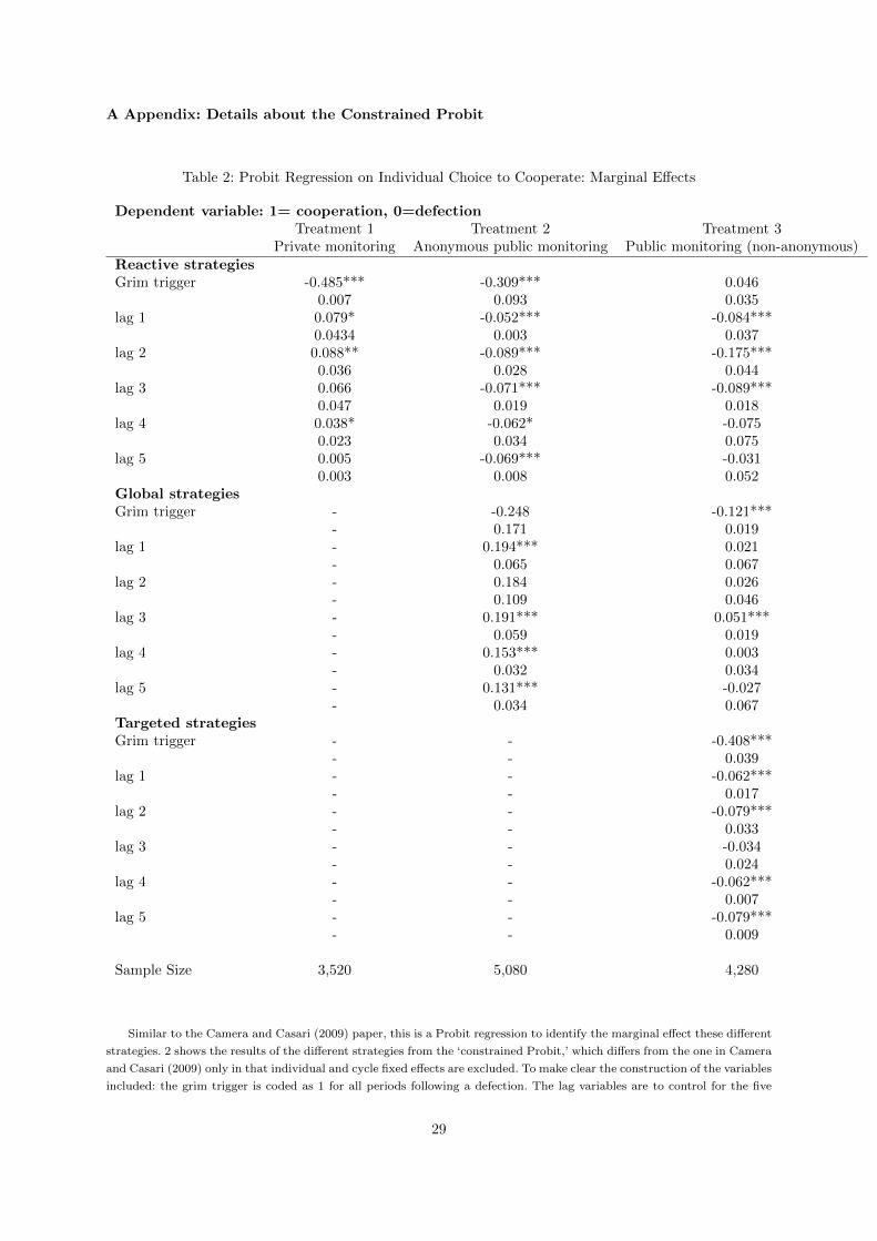
A Appendix: Details about the Constrained Probit
Table 2: Probit Regression on Individual Choice to Cooperate: Marginal Effects
Dependent variable: 1= cooperation, 0=defectionTreatment 1 Treatment 2 Treatment 3
Private monitoring Anonymous public monitoring Public monitoring (non-anonymous)Reactive strategiesGrim trigger -0.485*** -0.309*** 0.046
0.007 0.093 0.035lag 1 0.079* -0.052*** -0.084***
0.0434 0.003 0.037lag 2 0.088** -0.089*** -0.175***
0.036 0.028 0.044lag 3 0.066 -0.071*** -0.089***
0.047 0.019 0.018lag 4 0.038* -0.062* -0.075
0.023 0.034 0.075lag 5 0.005 -0.069*** -0.031
0.003 0.008 0.052Global strategiesGrim trigger - -0.248 -0.121***
- 0.171 0.019lag 1 - 0.194*** 0.021
- 0.065 0.067lag 2 - 0.184 0.026
- 0.109 0.046lag 3 - 0.191*** 0.051***
- 0.059 0.019lag 4 - 0.153*** 0.003
- 0.032 0.034lag 5 - 0.131*** -0.027
- 0.034 0.067Targeted strategiesGrim trigger - - -0.408***
- - 0.039lag 1 - - -0.062***
- - 0.017lag 2 - - -0.079***
- - 0.033lag 3 - - -0.034
- - 0.024lag 4 - - -0.062***
- - 0.007lag 5 - - -0.079***
- - 0.009
Sample Size 3,520 5,080 4,280
Similar to the Camera and Casari (2009) paper, this is a Probit regression to identify the marginal effect these different
strategies. 2 shows the results of the different strategies from the ‘constrained Probit,’ which differs from the one in Camera
and Casari (2009) only in that individual and cycle fixed effects are excluded. To make clear the construction of the variables
included: the grim trigger is coded as 1 for all periods following a defection. The lag variables are to control for the five
29
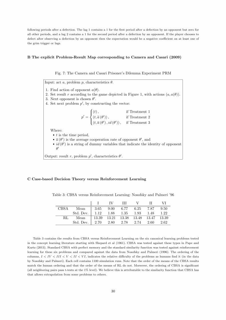
following periods after a defection. The lag 1 contains a 1 for the first period after a defection by an opponent but zero for
all other periods, and a lag 2 contains a 1 for the second period after a defection by an opponent. If the player chooses to
defect after observing a defection by an opponent then the expectation would be a negative coefficient on at least one of
the grim trigger or lags.
B The explicit Problem-Result Map corresponding to Camera and Casari (2009)
Fig. 7: The Camera and Casari Prisoner’s Dilemma Experiment PRM
Input: act a, problem p, characteristics θ.
1. Find action of opponent a(θ).2. Set result r according to the game depicted in Figure 1, with actions (a, a(θ)).3. Next opponent is chosen θ′.4. Set next problem p′, by constructing the vector:
p′ =
(t) , if Treatment 1
(t, a (θ′)) , if Treatment 2
(t, a (θ′) , id (θ′)) , if Treatment 3
Where:r t is the time period,r a (θ′) is the average cooperation rate of opponent θ′, andr id (θ′) is a string of dummy variables that indicate the identity of opponentθ′
Output: result r, problem p′, characteristics θ′.
C Case-based Decision Theory versus Reinforcement Learning
Table 3: CBSA versus Reinforcement Learning: Nosofsky and Palmeri ’96
I IV III V II VI
CBSA Mean 3.65 9.00 6.77 6.25 7.87 9.50Std. Dev. 1.12 1.88 1.35 1.93 1.48 1.22
RL Mean 13.39 13.21 13.38 13.48 13.47 13.39Std. Dev. 2.70 2.80 2.78 2.74 2.60 2.62
Table 3 contains the results from CBSA versus Reinforcement Learning on the six canonical learning problems tested
in the concept learning literature starting with Shepard et al (1961). CBSA was tested against these types in Pape and
Kurtz (2013). Standard CBSA with perfect memory and the standard similarity function was tested against reinforcement
learning for these six problems and compared against the data from Nosofsky and Palmeri (1996). The ordering of the
columns, I < IV < III < V < II < V I, indicates the relative difficulty of the problems as humans find it (in the data
by Nosofsky and Palmeri). Each cell contains 1100 simulation runs. Note that the order of the means of the CBSA results
match the human ordering and that the order of the means of RL do not. Moreover, the ordering of CBSA is significant
(all neighboring pairs pass t-tests at the 1% level). We believe this is attributable to the similarity function that CBSA has
that allows extrapolation from some problems to others.
30