Embed Size (px)
Citation preview
Alma Mater StudiorumUniversitá di Bologna
DOTTORATO DI RICERCA IN SCIENZE STATISTICHE
Ciclo XXVIII
Settore Concorsuale di afferenza: 13/D2 - STATISTICA ECONOMICA
Settore Scientifico disciplinare: SECS-S/03
Predicting nominal data
in presence of poor information.
An application to air tickets.
Coordinatore:Prof.ssa Alessandra Luati
Relatore:Prof. Andrea Guizzardi
Co-relatore:Prof. Michel Mouchart
Presentata da:Annalisa Stacchini
Esame finale anno: 2016

Data is not information. Information is not knowledge. And
knowledge is certainly not wisdom.
H. Gilbert Welch

AcknowledgementsI wish to acknowledge all the people that supported me during
the Ph.D. and the elaboration of the present thesis. First my
supervisor and co-supervisor, for the precious advices, the kind
availability and irreplaceable help they provided to me. Many
thanks to Professor David Draper for the truly kind hospitality at
UCSC, his great availability and all the suggestions. I also thank
all the professors of the Ph.D. board for having realized such a
valuable and fascinating program.
Then, I acknowledge Seneca, in particular Ercolino Ranieri and
Luigi Cristini, for having financed my scholarship, provided the
datasets and chosen a topic that opened original research prob-
lems. I thank Thot for the business-specific loss function.
A further acknowledge is for my Ph.D. mates, especially Flavio
Emanuele Pons, Saverio Ranciati and Matteo Farne’, who gave
me a lot of precious information and were always ready to answer
my often weird questions.
Finally, a very special thanks to all of my family, especially to my
father, mother and grandmother, for having supported me in all
the possible ways and with great affection.
Contents
Introduction 3
1 Context of the study 11
1.1 Travel Management Companies . . . . . . . . . . . 11
1.2 The commissioning TMC . . . . . . . . . . . . . . 13
1.3 Research Problems . . . . . . . . . . . . . . . . . 15
1.4 Literature Review . . . . . . . . . . . . . . . . . . 20
2 Qualitative investigation of the phenomenon 25
2.1 Methodological notes . . . . . . . . . . . . . . . . 25
2.2 The semi-structured interviews . . . . . . . . . . . 29
2.3 Description of participants and answers . . . . . . 30
2.4 Findings and guidelines for the quantitative study 38
3 Description of the dataset 43
3.1 The corporate database . . . . . . . . . . . . . . . 43
3.2 The composition of the dataset . . . . . . . . . . . 45
3.3 The variables . . . . . . . . . . . . . . . . . . . . 46
CONTENTS
3.4 Missing data and selection bias . . . . . . . . . . . 52
3.5 Descriptive statistics . . . . . . . . . . . . . . . . 58
4 Modelling the risk of non-fly 109
4.1 Simplifying the business problem . . . . . . . . . . 109
4.2 Models specification . . . . . . . . . . . . . . . . . 117
4.3 Notes on the Independence from Irrelevant Alter-
natives . . . . . . . . . . . . . . . . . . . . . . . . 123
4.4 Variables selection . . . . . . . . . . . . . . . . . . 128
4.5 Estimations resuts . . . . . . . . . . . . . . . . . . 134
5 Predicting air tickts’ outcomes 151
5.1 Prediction problems . . . . . . . . . . . . . . . . . 151
5.2 Guess-based predictions . . . . . . . . . . . . . . . 153
5.3 Economic evaluation of the forecasting performances158
5.4 A new classification algorithm . . . . . . . . . . . 163
5.5 Selecting ’primus inter pares’ . . . . . . . . . . . . 173
5.6 Results . . . . . . . . . . . . . . . . . . . . . . . . 179
Conclusions 187
Working bibliography 193

List of Figures
3.1 Dynamic of Non-Flown first tickets . . . . . . . . . 55
3.2 Sample temporal distribution of air tickets purchases 59
3.3 Sample spacial distribution of air tickets purchases 63
3.4 Sample composition by route . . . . . . . . . . . . 69
3.5 Sample composition by number of routes . . . . . 71
3.6 Sample composition by covered distance (Km) . . 71
3.7 Sample composition by ticket type . . . . . . . . . 72
3.8 Sample composition by type of itinerary . . . . . . 72
3.9 Sample composition by aircompany . . . . . . . . 74
3.10 Sample composition by Low Cost flights . . . . . . 76
3.11 Sample composition by class . . . . . . . . . . . . 76
3.12 Sample composition by typology of client company 77
3.13 Sample composition by business traveler’ sex . . . 78
3.14 Sample composition by business traveler’ age . . . 79
3.15 Sample composition by business traveler’ job . . . 80
3.16 Sample composition by type of contract . . . . . . 81
3.17 Distribution of Target-Buy by type of client company 82

LIST OF FIGURES
3.18 Distribution of Target-Buy by ticket type . . . . . 83
3.19 Distribution of Target-Buy by type of itinerary . . 84
3.20 Distribution of Target-Buy by low cost flights . . . 84
3.21 Distribution of Target-Buy by class . . . . . . . . 85
3.22 Distribution of Target-Buy by advance booking . . 85
List of Tables
3.1 Explanatory Variables . . . . . . . . . . . . . . . . 47
3.2 Missing data in explanatory variables . . . . . . . 53
3.3 Sample temporal distribution of air tickets purchases 60
3.4 Sample spacial distribution of air tickets purchases 64
3.5 Sample composition by route . . . . . . . . . . . . 69
3.6 Sample composition by number of routes (Km) . . 71
3.7 Sample compositionby by covered distance (Km) . 71
3.8 Sample composition by ticket type . . . . . . . . . 73
3.9 Sample composition by type of itinerary . . . . . . 73
3.10 Sample composition by aircompany . . . . . . . . 75
3.11 Sample composition by Low Cost flights . . . . . . 76
3.12 Sample composition by class . . . . . . . . . . . . 76
3.13 Sample composition by typology of client company 77
3.14 Sample composition by business traveler’ sex . . . 78
3.15 Sample composition by business traveler’ age . . . 79
3.16 Sample composition by business traveler’ job . . . 80
3.17 Sample composition by type of contract . . . . . . 81
LIST OF TABLES
3.18 Distribution of Target-Buy by type of client company 82
3.19 Distribution of Target-Buy by ticket type . . . . . 83
3.20 Distribution of Target-Buy by type of itinerary . . 84
3.21 Distribution of Target-Buy by low cost flights . . . 84
3.22 Distribution of Target-Buy by class . . . . . . . . 85
3.23 Distribution of Target-Buy by advance booking . . 87
3.24 Correlation Coefficients . . . . . . . . . . . . . . . 88
3.25 P-values of chi-squared tests . . . . . . . . . . . . 93
3.26 Differences from the marginal masses . . . . . . . 96
3.27 Specified independent variables . . . . . . . . . . . 105
4.1 Comparison of parametric and non-parametric vari-
ables selections results . . . . . . . . . . . . . . . . 134
4.2 Estimation output for Y1 . . . . . . . . . . . . . . 139
4.3 Estimation output for Y1 a . . . . . . . . . . . . . 140
4.4 Estimation output for Y1 b . . . . . . . . . . . . . 141
4.5 Estimation output for Y 2 | Y 1 . . . . . . . . . . . 142
4.6 Estimation output for Y 3 | Y 2 . . . . . . . . . . . 143
4.7 Estimation output for Y 3a | Y 2a . . . . . . . . . . 144
4.8 Estimation output for Y 3b | Y 2b . . . . . . . . . . 144
4.9 Estimation output for Y 5 | Y 3 . . . . . . . . . . . 145
4.10 Estimation output for Y 4 | Y 2 . . . . . . . . . . . 145
4.11 Estimation output for Y 4b | Y 2b . . . . . . . . . . 146
4.12 Estimation output for Y 6 | Y 1 . . . . . . . . . . . 147
LIST OF TABLES 1
5.1 Guess-based prediction: results for Model 1 + δD . 155
5.2 Guess-based prediction: results for bootstrapped
coefficients . . . . . . . . . . . . . . . . . . . . . . 157
5.3 Cost function . . . . . . . . . . . . . . . . . . . . 161
5.4 Loss function . . . . . . . . . . . . . . . . . . . . . 161
5.5 Results for Y1 . . . . . . . . . . . . . . . . . . . . 171
5.6 Results: Dynamic forecasts . . . . . . . . . . . . . 183

2 LIST OF TABLES
Introduction
The present thesis is written upon commission by a Travel Man-
agement Company (TMC). Among the various services and prod-
ucts offered by the TMC, an important business is constituted by
the brokerage of business flights. A special contract, developed
by the TMC, provides that the client company can agree to pay a
fixed price for any flight with the wanted characteristics (on board
class, route, airline). This arrangement puts the TMC in the po-
sition in which corporate travel departments are normally, having
to minimize the cost of flights.
In fact, the management of business travel costs is becoming an
important issue for more and more corporations, in increasingly
globalized business environments. While in companies that do not
require numerous business flights the ticket is often booked by the
traveler himself (often in view of his comfort and frequent flyer
program), corporations needing many flights tend to formulate a
corporate travel policy, aiming at minimizing the cost of flights.
Whence the need of a decision-making strategy able to help in this
complex task, especially nowadays, when the bargaining power of
3
4 LIST OF TABLES
corporations (with respect to the airlines) is very low and it is be-
coming impossible to get real quantity discounts, due to the global
agreements among airlines and their strong revenue management
strategies.
Most corporate travel departments, at least in Italy, assume
that the best buy strategy consists in purchasing always the cheap-
est ticket, also considering that the difference in price, between
fares, is great. But does ’best buy’ mean buying always the cheap-
est ticket? Considering that the cheapest air fare is the fixed one,
not allowing changes nor refund, whether the traveler changes or
renounces to the flight, the cheapest first issued ticket leads to
a higher overall cost of the flight, than that allowed by a more
expensive but more flexible fare.
While choosing the cheapest air ticket is easy, as the prices of
different fares are known and comparable at the time of book-
ing, getting the needed flight at the lowest possible cost is not
that straightforward. In fact, the cost of business flights does not
depend only on the price of the first booked ticket, but also, all
other conditions (class, route, date, time, airline) equal, on the
chosen fare and on the behavior of the business traveler, which in
turn will determine which fare was the optimal one (at the time
of booking). The more flexible the fare, the higher the price, the
lower the cost of changes and renounces.
If, at the time of booking, a leisure traveler does not know for

LIST OF TABLES 5
sure whether he will change date or destination, or will have to
renounce to the journey, a corporate travel department is even
more uncertain about the business traveler’s behavior. In fact, a
leisure traveler can guess quite reliably that he will (not) flow the
initially purchased ticket, because he has a wide knowledge of his
personal, familiar and professional situation (for example, if he
books a flight for a holiday, but his mother-in-law is seriously sick
and may need assistance, he will opt for a refundable fare).
Contrarily, in a business context, the traveler undergoes the
events, which are often unforeseen. For example, he could have
to change the date of a flight, because a client needs to postpone
or antedate a meeting, or he may have to renounce, because of
an epidemic in the destination. Such a broad uncertainty im-
plies that the cost of flight is unknown at the time of booking, so
that the corporate travel department cannot minimize it directly.
Therefore, ’best buy’ means choosing the optimal fare minimizing
the value of the cost of flight, as expected based on the available
information, able to help predicting how the traveler will behave.
Therefore, this business problem requires a statistical solution,
because of the uncertainty about the travelers’ behavior, which
can be modeled as a nominal random variable. The objective of
the present work is to provide such a solution. Appearently, the
one at hand, is a simple decision-making problem, under mini-
mization constraints. The action space is constituted by the set
6 LIST OF TABLES
of fares among which the purchasing agent can choose. The con-
straints consists in deciding for the fare minimizing the expected
value of the cost of flights.
Indeed, the task is made especially difficult by the poor infor-
mation available. In fact, the corporate dataset, provided by the
TMC, was collected for purposes different from that of the inves-
tigation. Therefore crucial data are missing, beginning with the
fares of observed tickets, their price and the penalties for changes.
This lack of necessary information makes impossible to define the
action space and to compute the expected value of the cost of
flights.
Moreover, observations cover a too limited time span, in par-
ticular the estimation sample spans just seven months, so that
no eventual time component can be detected. In addition, the
hierarchical structure of data (tickets bought for a traveler, trav-
elers working for a company, company belonging to a certain
macro−category) cannot be modeled, because the dataset is greatly
unbalanced, due to the 80/20 rule of sales, and the identifiers
of groups are missing in too many cases and it is not even sure
that non-identifiable tickets do not actually belong to an identified
group.
Finally, most of the available data refer to the characteristics
of the ticket and the flight, that are not well correlated with the
behavior of the business traveler. Information about the flyer’s
LIST OF TABLES 7
professional status, personal and family situation, and its com-
pany’s business would have been very useful to predict his behav-
ior and give an indication about which fare to choose. Their lack
causes serious forecasting problems, also considering that it is not
possible to perform many elaborations on nominal data, due to
their qualitative and non-ordinal nature.
As a consequence, the present work aims at developing alter-
native solutions, useful for predicting nominal data in border-line
situations of this kind, where the available information is so poor
that the traditional statistical techniques need to be integrated.
Thus, the original contributions of this thesis, to the prediction of
nominal data in presence of poor information, are three.
First, proposing an easy method to incorporate a guess about
a non−estimable effect, of a non−observable variable, directly
into an estimated model. Second, developing a classification algo-
rithm, able to extract from the whole matrix of predicted proba-
bilities, both the latitudinal and longitudinal information, able to
correctly classify at least some of the most economically relevant
outcomes, that are also the greatly less frequently observed ones.
Last, propounding a new measure of forecasting accuracy to se-
lect the best predictor among a set of models appearently with
identical predictive performance, as assessed through the extant
statistical methods.
While the importance of the present work, from the phenomenic
8 LIST OF TABLES
perspective, consists in providing a statistical tool suggesting the
TMC which one is the best fare to buy. But also in providing a
formal approach for helping corporate travel management depart-
ments minimizing business travel costs. More generally, in show-
ing that ’best-buy’ does not always mean choosing the cheapest
fare.
This thesis is articulated as follows. The context of the study
is first described, providing a digression about the birth and the
development of companies specialized in business travel manage-
ment, an illustration of the characteristics of the specific TMC
commissioning this work, a formalization of the main research
problem and a review of the little extant literature. A qualitative
study of the business problem follows. Some methodological notes
are premised, then the semi-structured interviews and the panel
of participants are described, finally the findings and the obtained
guidelines for the subsequent quantitative study are presented.
The dissertation continues illustrating the corporate database,
its composition, the specification of the variables, the problems of
missing data and some sample statistics. Chapter four deals with
modeling the phenomenon under investigation: first the business
problem is simplified, then a functional form is chosen, some notes
on the important assumption of independence from irrelevant al-
ternatives are discussed, explanatory variables are selected and
estimation outputs are commented.
LIST OF TABLES 9
Chapter five is the most innovative one: after detecting the
causes of the emerged prediction problems, some alternative solu-
tions are developed. First an easy method for vague guess-based
prediction, then a business-specific loss function computable with
the few information at disposal, employable for comparing the
predictors’ economic performance. In addition, a new classifica-
tion algorithm and a measure of forecasting capability considering
the estimated probabilities. Finally results are presented and the
thesis is concluded.

10 LIST OF TABLES

Chapter 1
Context of the study
1.1 Travel Management Companies
The present Ph.D. thesis was commissioned by Seneca, the Travel
Management Company (TMC) which funded my Ph.D. scholar-
ship. Contextualizing the research problems, presented in the fol-
lowing chapter, allows to understand the implications and impor-
tance of the study, because it is very operational in nature and
tightly related the business activity of the TMC. As TMCs are
a relatively new form of intermediaries in the travel market, it
is worth spending some words to explain what they exactly are,
which is the commercial room on which they rose and how they
differ from the well known travel agencies.
A TMC can be seen as an evolution of the traditional travel
agency, in the sense that it is specialized in business travel and,
besides the usual intermediation activity, offers a wide set of travel
management services. TMCs arose from the change in the rela-
11
12 1.#1
tionship between airline companies and travel agents, begun in the
USA in the second half of the nineties, when the economic reces-
sion induced the airlines to reduce costs (Levere, 2000). In fact,
about the 17% of airlines’ total operating costs in 2000 was related
to distribution, the third largest cost, after labor and fuel (Inter-
national Air Transport Association, 2000). Recently these costs
are steadily decreasing (see: Air Transport Association, 2014).
As the progress of information technology (IT) made search
and booking procedures much easier and cheaper, travel agencies’
commissions, accounting for more than the 10% of the air com-
panies’ distribution cost in 1993 (currently about the 8%), were
questioned and slashed by the airlines. Following the American
companies, soon also European carriers reduced agents’ commis-
sion fees, starting from the British Airways, in 1998 (Alamdari,
2002).
Gradually, the contraction of travel agents’revenues was exac-
erbated by the increase in the bargaining power of customers. In
fact, more and more individuals and small companies prefer di-
rect contact with airlines, or online booking sites, automatically
comparing flights and prices. While big enterprises, became aware
of the importance of managing travel expenses, started adopting
self-tailored travel policies and buying directly from the airlines,
to get volume discounts. Therefore travel agencies reshaped their
business and often specialized in leisure tourism, focusing on the

1.2#1 13
more remunerative supply of vacation packages, or in business
travel, offering consultancy services to help companies developing
and enforcing travel management policies, in order to optimize
their travel spending.
The second choice characterizes TMCs, which mainly provide:
up-to-the minute reports on travel patterns of employees, reports
on the effectiveness of travel policies, advice on complicated itineraries,
consultancy on travel data management, day-today operations of
the corporate travel program, advice for planning and budgeting,
traveler safety and security, and credit-card management. Thus,
currently TMCs’ revenues are mainly generated by the commis-
sions charged for such services, on the supply of which, rather than
on intermediation, they compete against their rivals worldwide.
However, some companies build their competitive advantage
also on the offer of innovative intermediation contracts, adding,
to the traditional distributional activity, conditions increasing the
value for the clients. Whence the importance, for TMCs, of re-
search and innovation, both of produced services and of produc-
tion processes, as it is the objective of the present work.
1.2 The commissioning TMC
Seneca is an experienced TMC, for over 20 years one of the top
business travel agencies in Italy, characterized by a constant com-

14 1.#1
mitment to research and development of both new services, in
order to anticipate the market changes and widen its offer, and
new production processes, for increasing its operational efficiency.
Seneca’offer mainly consists of:
• Business travel services,
• Business hotel services,
• Travel Management services,
• Hotel representation,
• IT systems,
• A new Global Distribution System for hotels,
• Target Buy purchasing pattern.
The Target Buy contract is one of the most appealing Seneca’ s
innovations. It provides that the client and the TMC bargain the
target price (for a single or set of air routes, for a category of ho-
tel room, etc.) at the signing of the contract.Then, the client will
always pay that same target price for that product, discharging
the risk of price variations on the TMC, which will buy at the
spot price from the providers. Thus, the client has the advantage
of purchasing at stuck prices, hedging the risk of fluctuations in
the travel expenses, and of knowing in advance the amount of the
cost, making the travel budgeting more certain and its manage-
ment easier. Moreover, if the customer renounces to the flight, or
1.3#1 15
to the hotel stay, at any time prior to departure, the TMC refunds
the full target price. The client is also allowed to change the time
and/or place of flight/overnight stay, completely free of charge, or
paying a fixed penalty, if provided in the contract. Therefore, this
contract is very risky for the TMC, that has to be very careful in
setting the target price and try to manage the risk of change and
waiver.
Developing an innovation in the purchasing process of air tick-
ets, able to minimize the economic losses due to the risk of change
and waiver of air tickets, is the aim that Seneca set for the present
thesis. The usefulness of such an innovation is not only circum-
scribed to the Target Buy contracts, but extends to the whole
activity of air tickets intermediation. In fact, as it is explained in
the following section, for the same route, date, advance booking
and class (determined by the client), it is possible to buy various
tickets, differing in the degree of flexibility and price. Thus, even
for non-Target Buy clients, Seneca can choose which one to buy
and the economic result of each transaction depends on the kind
of purchased ticket and the risk of change and waiver.
1.3 Research Problems
Given the context of the present thesis and the requirement of the
commissioning TMC, it is clear that this work develops around
16 1.#1
the solution of a very concrete and firm-specific problem, which
poses itself operational and research problems, from which more
general methodological issues, about applying Statistics to busi-
ness problem solving, stem.
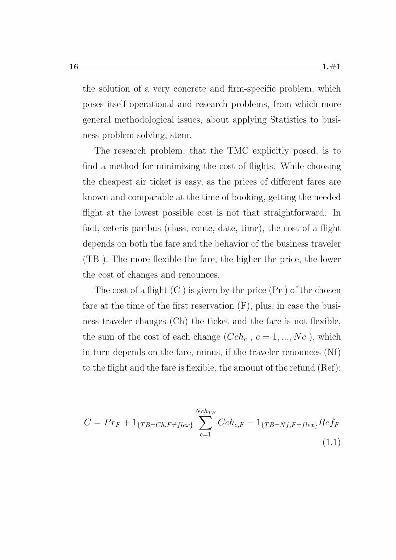
The research problem, that the TMC explicitly posed, is to
find a method for minimizing the cost of flights. While choosing
the cheapest air ticket is easy, as the prices of different fares are
known and comparable at the time of booking, getting the needed
flight at the lowest possible cost is not that straightforward. In
fact, ceteris paribus (class, route, date, time), the cost of a flight
depends on both the fare and the behavior of the business traveler
(TB ). The more flexible the fare, the higher the price, the lower
the cost of changes and renounces.
The cost of a flight (C ) is given by the price (Pr ) of the chosen
fare at the time of the first reservation (F), plus, in case the busi-
ness traveler changes (Ch) the ticket and the fare is not flexible,
the sum of the cost of each change (Cchc , c = 1, ..., Nc ), which
in turn depends on the fare, minus, if the traveler renounces (Nf)
to the flight and the fare is flexible, the amount of the refund (Ref):
C = PrF + 1TB=Ch,F 6=flex
NchTB∑c=1
Cchc,F − 1TB=Nf,F=flexRefF
(1.1)
1.3#1 17
where 1TB=Ch,F 6=flex is an indicator function, equal to 1 if the
business traveler changes the first issued ticket and the fare is
not flexible, 0 otherwise. 1TB=Nf,F=flex is an indicator function,
equal to 1 if the business traveler renounces to the flight and the
fare is flexible, 0 otherwise.
If, at the time of booking, a leisure traveler does not know for
sure whether he will change date or destination, or will have to
renounce to the journey, a TMC (or, within a ’client’ company,
is even more uncertain about the business traveler’ s behavior.
In fact, a leisure traveler can guess quite reliably that he will
(not) flow the initially purchased ticket, because he has a wide
knowledge of his personal, familiar and professional situation (for
example, if he books a flight for a holiday, but his mother-in-law
is seriously sick and may need assistance, he will opt for a refund-
able fare).
Contrarily, in a business context, the traveler undergoes the
events, which are often unforeseen. For example, he could have
to change the date of a flight, because a client needs to postpone
or antedate a meeting, or he may have to renounce, because of an
epidemic in the destination.
Such a broad uncertainty implies that the cost of flight is un-
known at the time of booking, so that the TMC (or the corporate
travel department) cannot minimize it directly. Therefore, ’best
18 1.#1
buy’ means choosing the optimal fare (F∗) minimizing the value
of the cost of flight, as expected based on the available informa-
tion (X), able to help predicting how the traveler will behave:
F∗ : ETB[CF∗ | X] = minETB[CF | X] (1.2)
ETB[CF | X] = PrF+1F 6=flex
Nch∑c=1
P [TB = Chc | X]Cchc,F−1F=flexP [TB = Nf | X]RefF
(1.3)
where P [TB] is the probability of business traveler’s behavior, or, seen fromthe TMC’s perspective, the probability of tickets’ outcomes.
Thus, for making the optimal purchasing decision, it is necessary to es-timate P [TB | X]. Clearly, the optimal solution would be obtained if Xwere able to reduce the uncertainty about TB to the mere statistical error.Therefore, modelling and predicting the ’risk of non-fly’ is the first researchproblem addressed in this thesis.
The other research problems derive from the poorness of the informa-tion available to perform this, otherwise easy, task. A first issue concernsthe specification of variables. Given that a few client companies purchasemost of the flights, that are nearly identical (same X values) and, amongnumerous tickes, just very few are not flown; that most of the available dataabout independent variables is categorical, with numerous classes for most ofthem and a highly concentrated distribution; and that the literature on thistopic is neraly null, there is no guidance about how to specify explanatoryvariables and to aggregate the too many levels.
A specification problem emerges also with reference to the dependent
1.3#1 19
variable. In fact, the number of possible changes is virtually infinite andthey can be either total or partial. So a simplification of the events spacemust be done. However, the possible tickets’ outcomes are still too manyand, if specified as levels of a single dependent variable, would make anymodel unidentifiable.
In addition, most of the available variables are not well correlated withthe traveler’s behavior, so just a very small proportion of its variability canbe explained. This problem is due to the fact that the database has beencollected for purposes different from that of the investigation, but also tocost and privacy constraints, often found in business contexts. Furthermore,the estimation sample covers only seven month, so that no eventual timecomponent can be modeled. Moreover, the mentioned high unbalance of thepanel structure of the dataset does not allow to specify hierarchical models.
As a consequence, the discriminatory power of available explanatory vari-ables is extremely low and the forecasting performance of estimable modelsis very disappointing. Thus, a further research problem, addressed in thisthesis, refers to the development of alternative solutions to improve the pre-dictive capability of the models.
In addition, for choosing the optimal fare, minimizing the cost of flights,it would be necessary to compute the expected value of such a cost. This ispossible if the price, the penalty for changes and the fare of observed ticketsare known, but in the available dataset this information is missing in toomany cases, so that this traditional approach cannot be adopted.
Therefore, after estimating the probability of tickets’ outcomes, it is nec-essary to define an optimal decision rule, as a function of such probability,ready-to-use within the everyday working practice of the TMC. Where the’optimal’ rule is the one maximizing the economic result of intermediationoperations for Seneca. Thus, a method to compare the economic performanceof candidate predictor models with that of the current business practice, inabsence of sufficient economic information, must be proposed. In fact, in
20 1.#1
business environments a probability value acquires a meaning in relation tothe economic output of a decision based on such value, rather than in com-parison with other values.
For example, whether it is found that the probability of changing theticket for business travelers, making trips with certain characteristics, is 60%and that of flying is 40%, should the purchasing clerk buy a, more expen-sive, flexible ticket, instead of a fixed one, because the probability of changeis (slightly) higher than that on non-change? The issue is: will the highercost be worth that 10% of extra probability? Thus, formulating the optimaldecision rule, operationalizing the estimates of the risk of non-fly, obtainedthrough different models (as no literature suggests how to model the phe-nomenon of interest), and selecting the best performing one, in terms ofeconomic utility for the TMC, is the last research problem, addressed in thisthesis.
1.4 Literature Review
The management of business travel costs is becoming an important issuefor more and more corporations, in increasingly globalized business environ-ments. While in companies that do not require numerous business flights theticket is often booked by the traveler himself (often in view of his comfort andfrequent flyer program), corporations needing many flights tend to formulatea corporate travel policy, aiming at maximizing travel security end efficiency,while minimizing the cost of business travel.
With reference to the air tickets, the capability of minimizing the costof flights largely depends on the choice of the optimal fare. Many studies(Turismo d’affari, 2014) highlight that, in this prolonged period of economicdifficulty for Italian enterprises, "best" buy become synonym of "cheapestticket". In fact, many corporate travel policies prescribe to purchase always
1.4#1 21
the cheapest fare available at the time of booking, also considering that thedifference in price, between fares, is great. This evidence is also supportedby the increase of business flights operated by low cost airlines (see: Amexinvestigations).
But Proussaloglou and Koppelman (1999) found evidence that appears tocontrast with this hypothesis. Their study about how the air travelers chooseamong different carriers, flights, and fare classes, shows that both businessand leisure travelers are willing to pay a premium for the flexibility offeredby the most expensive fares. Fourie and Lubbe (2006) investigated the deter-minants of the business travelers’ choice between low-fare and full-service aircompanies, in South Africa. They found evidence that, except for the price,the decision is led by considerations about comforts and service level, thatare surely important for the traveler, but, for corporate travel departments,not as crucial as the cost management.
Hence, the question, whether best buy means buying always the cheapestticket, is open and crucial. The present study suggest to face the choice of theoptimal fare considering that the overall cost of a business flight is composedby the price of the first issuance, plus the cost of the required flexibility.The first component can be managed by bargaining volume discounts withthe airlines, although the progressively more widespread diffusion of revenuemanagement systems and the global agreements between air companies low-ered the bargaining power of client companies, leaving the business travelmanagement the only opportunity to contract a percentage reduction on the(expensive) business fare, unilaterally defined by the airline.The second com-ponent can be controlled by forecasting the travel behavior.
In the extant literature, this issue is addressed from the airlines’ perspec-tive (Gorin et al, 2012; Bartke et al, 2012), aiming at developing pricingmethods minimizing the negative impact, on their margins, of cancellations(for unrestricted fares) and rebooking (for restricted fares) close to the de-parture. To the best of our knowledge, no study considers the prediction of
22 1.#1
the outcome of booking (change, no-show, cancellation), in the definition of’best buy’, from the perspective of corporate travel departments (or TMCs).
Indeed, literature deals with sunk costs (Park and Jang, 2014), or focuseson changes and waivers as determinants of the choice between low-fare andfull-service air companies (Fourie and Lubbe 2006). Further papers concernthe choice of the airline (Nako, 2992), the influence of time and service qual-ity on air travel demand (Anderson, and Kraus, 1981), factors influencingprice elasticity (see: Brons et al, 2002).
More in general, literature about the market of air tickets mainly dealswith the mounting use of the internet for online booking. It analyses thenew services, pulled by this phenomenon, offered by the air companies (Lawand Leung, 2000), the distributors (Bitner and Booms, 1982) and accessoryservices providers (Law and Chang, 2007); the strategic and economic conse-quences of online booking for the airlines (Yoon et al, 2006); the consumers’perception of the risk of employing the new media (Kim et al, 2009) and,conversely, the determinants of their trust (Alam and Yasin, 2010).
The prices of air tickets have been considered in a few works, investi-gating, from the perspective of the airline, the influences of the compaies’financial situation (Borenstein and Rose, 1995 ), services provision costs anddemand level (Botimer and Belobaba, 1999), and price wars (Brady and Cun-ningham, 2001) on pricing, but mainly on the theoretical level.
But the most interesting researches, for the aim of the present thesis, arethose analysing air tickets’ prices through hedonic-price and regression mod-els, because they highlight the attributes of the ticket/flight, which play amajor role in determining the fares. In particular, for air tickets distributedthrough ’traditional’ channels, advance purchase, airline, destination and sat-urday night stay have been found to crucially influence prices (Vowles, 2000;Wallenberg, 2000).
Along with these characteristics, also online travel agent, time windowsfor departing and arrivals (Clemons et al, 2002), kind of connection, fuel

1.4#1 23
price, peak hour of departure, seasonal dynamic, seat class (Chen, 2002),and recently maximum stay, refundability, restrictions on flights (Lin et al,2009) were investigated, resulting important for price determination. How-ever, these analysis are limited to tickets homogeneous with respect to theflight route and class. Moreover the different ticket conditions, especiallywith reference to the degree of flexibility, within the same class, are aggre-gated.
Indeed, the lack of more complete empirical studies on the market of airtickets is not that surprising, given the complexity of obtainable data. Infact, it has been proved that identical tickets can be bought at very differentprices from different online distributors, evidences pointing at relevant im-perfections in the online air ticket market (Clay et al, 2001; Lin et al, 2009).
Another difficulty, found in the present work and implicitly shared by thequoted studies, consists in classifying tickets based on their degree of flexi-bility, which is of special importance to business travelers (Mason and Gray,1999), because different airlines offer different sets of alternatives, which arenot fully comparable across operators. Moreover, often these conditions areaffected by the uncertainty deriving from clauses providing that the penaltieswill be computed (who knows how) at the moment of ticket change/waiver.
In brief, the rare literature of interest for the present work confirms whatis observed in the database at hand (see chapter 4): that the tickets’ con-tractual conditions are extremely various, because each single airline definesits own typologies of fares and on-board booking classes, which jointly de-termine the degree of flexibility of the ticket and the differences in cost andservices between them.
Each airline company has its own pricing policy, which can vary in timeand space, and often does not offer all the listed conditions on every flight,while sometimes those conditions are available through insurance bills, man-aged by third-party insurance companies. This situation is made more com-plicated by the different prices applied to identical tickets by online travel

24 1.#1
agents. Although generally, a fully refundable ticket (which can be entirelyrefunded at any time by the airlines) costs about 50% more than a non-refundable one (McAfee and Velde, 2006), the differences in prices due to thedifferent degrees of tickets flexibility can vary a lot, even within the same air-line. These are the main reasons why the market of air tickets seems rathera ’jungle’.

Chapter 2
Qualitative investigation of the phe-
nomenon
2.1 Methodological notes
In Social Sciences and Medicine qualitative research is widely spreading (e.g.Wilfried and Tarnai, 1999; Fossey et al, 2002), but it can be very useful alsoin other fields of study, especially when working on a problem for the solutionof which no literature is available, as in the present case. The qualitative ap-proach aims at analyzing a problem in depth (rather than ’in width’ as it isthe case of the quantitative approach) involving a limited number of subjects,belonging to a certain group, defined on the basis of variables likely to beassociated with the phenomenon of interest (Wunsch et al, 2014), contrarilyto what happens in quantitative statistical sampling design.
Once overcome the long lasting dichotomy between ’comprehension’ and’explanation’ of phenomena (Dilthey, 1883), qualitative and quantitativemethods are finally being recognized as complementary (Malterud, 2001;Wunsch et al, 2014). The main purposes of qualitative research are (Fosseyet al, 2002):
• to improve the understanding of the object of investigation from the
25
26 2.#1
perspective of the involved subjects;
• to explore the meanings of phenomena as directly experienced by indi-vidual themselves, within the context of their life and social environ-ment;
• to lead designing of further, eventually quantitative, research.
As highlighted by Gordon and Smith (2004), qualitative investigation is anespecially serviceable tool when addressing phenomena characterized by mul-tiple causal mechanisms, in which different causes can produce the same out-come and it is not possible to observe which mechanism generated each effectin the available sample.
This is the case of the present work: different unobserved motivationsare likely to lead business travelers to fly or not to fly. The available quan-titative data allow to analyze the behavior of a (relatively) great number oftravelers, thus promising to find constant patterns, which can be general-ized to the whole population of business travelers, to forecast their choices.But no information about the actual motivations of changes, refunds, flights,non-flights is available. These motivations are (as shown in the following)the actual causes of tickets’ outcomes and can be (hopefully) related to someof the candidate explanatory variables at hand, but from the dataset it isimpossible to find out which variables are related in which way to the ’realcauses’ of the events of interests. While it is such a knowledge that shouldlead the modelling of the probability of non-fly. Whence the opportunity torealize a deeper qualitative study on just a few individuals, which can shedlight on the causal mechanisms hidden behind the business travelers’ behav-ior.
The first crucial issue, in qualitative studies, is the definition of themethod to employ. The main alternatives are: observation, written ques-tionnaire, oral/written interviews. In the present case, the first alternative isunviable, because it is not possible to follow business travelers at work. As
2.1#1 27
the primary purpose of this qualitative research is to explore hypotheses onvariables, for planning the subsequent quantitative study and implement asound statistical strategy, a semistructured interviews appear to be the opti-mal choice (Malterud, 2001). In fact, the less pre-determined is the interview,the less the researcher’s subjectivity, prejudices and a priori opinions affectthe study. The idea is to let participants to express the ’lived’ meaning oftheir own experience of the actual context of ’business flying’, as freely aspossible.
As an appropriate sampling methodology is fundamental for quantitativestudies to be reliable, the choice of the units of analysis is possibly even morecrucial in qualitative research, because just a few individuals are selected.Dealing with sampling, it is to be noted that in the present case there isno sampling, but census of all the tickets intermediated by Seneca since thedata collection became possible, as the reference population is composed byall the tickets purchased by the TMC and, just by extension, to that of busi-ness travelers, of the behavior of which the tickets’ outcomes are ’objectivecorrelates’.
However, turning to qualitative analysis, Graneheimand Lundmanl (2004)suggested that the selection of participants living different experiences in-creases the potential of widen the understanding of the research question toa variety of aspects. Moreover, in order to enhance the transferability of find-ings, it is worth of providing an exaustive description of participants’ culturalbackground, context and subjective characteristics. Thus, the present workproceeds as suggested, to the extent to which it is possible, because it is noteasy to realize depth interviews with different frequent business flyers.
In fact, business travelers are not even minimally remunerated for theparticipation to the interview, which is motivated solely by friendship, there-fore individuals have been chosen among my friends, based on the frequencyof flights they do for work. Another difficulty consists in the fact that fre-quent flyers spend a lot of both spare and working time for traveling, thus

28 2.#1
they have very few time left for other purposes, like answering interviews.Once chosen the method and selected the participants to the study, the
issue of how to use the obtained information arises. As highlighted by Mal-terud (2001), coding such information as numerical variables and processingit through statistical techniques for qualitative data is not the most appro-priated method. In fact, the scientific logic, on which statistical techniquesrely (especially the requirement of independence of the variables used forthe selection on the model’s dependent one) are incompatible with the ’non-representativity’ of the interviewed group and, as the interview is semistruc-tured and mainly informal, with the circumstance that questions are notasked nor answered in standardized way (thus not liable to form homoge-neous categories). Thus, retrieved information is ’qualitatively’ employed,without formal elaboration.
It is to be noted that this qualitative analysis is not to be employed onlybefore the quantitative study of the phenomenon under investigation, but itis also useful after that, to better interpreting the meaning and implicationsof findings. Thus, the actual pattern of integrating qualitative and quantita-tive analysis, in the present work, can be named ’triangulation’: "The aimof triangulation is to increase the understanding of complex phenomena, notcriteria-based validation, in which agreement among different sources con-firms validity." (Malterud, 2001, p. 487). In particular, this approach refersto the practice of non-mixing qualitative and quantitative data in modellingthe phenomenon, but respecting the difference in nature and in the statisticalcharacteristics of the two type of informations. This imply integrating themin a meta-analysis (or secondary analysis), leading to mutual validation ofthe results of both.
2.2#1 29
2.2 The semi-structured interviews
The interviews were realized mainly through a popular social network, be-cause participating business travelers were in different counties, at the time ofthe interview. Only an interview was realized in presence, orally. The inter-views were informal, all followed a common draft, but in a very flexible way,as the questions were formulated as a function of previous answers, consis-tently with the business traveler profile which was gradually being outlined.The draft is the following:
1. How many flights do you do for business, on average, per month?
2. Is there, in your company/institution, a (or more) person assigned tothe task of buying or reserving flights? Or do you do it by yourself?
3. If it happens that you waiver a flight, for which you already bought theticket, which are the motivations of the renounce?
4. If it happens that you waiver a flight, for which you already bought theticket and are entitled to refund, but you (or the person assigned to thistask) do not ask the refund, which are the motivations of the renounceto refund?
5. If it happens that you completely change the date or the routes (or both)of a flight, which are the motivations of the change?
6. When you hold an air ticket including different routes and/or a roundtrip, if it happens that you change just a part of the ticket (e.g. youfly only to one or more destinations, but change the other/s, or youreturn earlier, or change one or more, but not all the dates) which arethe motivations of the change?
7. Which of the following factors:
30 2.#1
• the destination of the flight,
• the weekday of departure,
• the month of departure,
• your professional status within the company (institution)’s hierar-chy,
• the reserved on-board class,
influence the decision of:
• Completely change the air ticket?
• Partially change the air ticket?
• Completely waiver the flight?
• Partially waiver the flight?
The anonimity was, of course, explicitly guaranteed to all the participants,along with the guarantee that none of the provided information will be dis-closed to anyone related to their company/institution.
The time of the interviewed varied a lot, from case to case, depend-ing on how many questions were excluded for consistency with previous an-swers (e.g. if a business traveler stated that he never changes ticket, all thequestions about changes were skipped). However, the time of the interviewnever exceeded 20 minutes, as all the respondents’ professional status, refer-ence company/institution and socio-demographic information were alreadyknown.
2.3 Description of participants and answers
Seven business travelers were selected to participate to the interview, basedon the high number of times they fly for work, which is a characteristic surelyrelated to the variables of interest (the more times a business traveler flies,
2.3#1 31
the higher, theoretically, may be the probability that, sometimes, he changesor waivers or asks refund of the ticket). The participants have various jobpositions in different companies and institutions, with headquarters in vari-ous countries. Unfortunately, they are all males, as it is rare to know womenfrequently flying for work (maybe due to familiar reasons), and their ageis rather homogeneous, as it is usual in friendship environments. Moreover,most of them are single, as it is often the case of people traveling a great partof their time. For sake of easiness of exposition, each participant is indicatedwith a letter.
Participant A is a 30 years old entrepreneur, with a degree in History.His company is located in Brazil and deals with export and sale of made-in-Italy clothing. He is single and lives in Italy. He flies to Brazil, to staythere at least 1 week and 3 weeks maximum, and comes back to Italy once amonth, on average. He purchases air tickets by himself, or together with hisassociate. As the company is still a start-up, participant A is very carefulin controlling expenses, so he prefers buying last-minutes offers, or low costflights in low demand (thus lower cost) periods of the year.He can fly whenever the ticket is cheaper because, being the owner of thecompany, he is absolutely autonomous in his working decision and travellingchoices. He has never changed an air ticket, neither totally, nor partially,since he started the business activity, to avoid increases of travel expenses.Nonetheless, he said that, whether he made a change, it would be surelydue to serious familiar reasons and the very few times, when he waivers aflight, it is because of motivations related to his origin family. Consistently,the destination of the flight, which is always the same for him, the month ofdeparture, which is indifferent to him, the reserved on-board class, which isalways the cheapest, do not influence his travelling decisions.In fact, participant A declared that only the weekday of departure influencesthe probability that he partially changes the flight, because, within his fam-ily, familiar meetings and events are organized in the weekend and he does
32 2.#1
not want to miss them. Thus, if the cheapest round trip ticket provided adate of return in the weekend, he would change such a date, in order to at-tend to his family’s event. When asked explicitly, participant A denied thathis professional status influences his travelling choices.
Participant B is a 37 years old professional, with a degree in Tourism Eco-nomics. In particular, he is marketing and management advisor for the hotelindustry. He is single, lives and works in Italy, he flies 0.5 times per month,on average, staying at the destination a variable length of time, from a fewdays to various weeks. He purchases air tickets by himself, mainly for short-haul national flights. When he changes ticket, he changes it totally, becauseof his clients’ modified schedules. But when he waivers a flight, it can bedue to various motivations: origin family needs, his clients’ requests, hitchesoccurred during his activity. In fact, his work must be approved by hotels’owners and managers, thus an activity which he planned to accomplish in acertain time, often requires more days, to satisfy the client, therefore plannedjourneys must be postponed.Often it happens that participant B renounces to ask a refund to which he isentitled, because he thinks that the procedures to obtain it require too longtime, compared to the small amount of money involved. As he does not flyvery often, he does not care too much for the travelling expenses, thus theon-board class has no influence on his travelling decisions. He said that alsothe month of departure is indifferent, as changes and waivers are determinedby unpredictable snags. He thinks that also his job position is ininfluent onthe probability of changing or renouncing to flights, but eventually it is noton his tendency not to ask refund, as the time he spend in consulting is soremunerative that he is not willing to divert it on the application procedurefor refund, while, if he did a less remunerative job, he could evaluate such anaspect differently.The weekday of departure and the destination of the flight are important fac-tors in determining whether he changes ticket or not, in fact no hitch occurs
2.3#1 33
to him during the weekend, although his clients can work, as it is usual inthe tourism field, because he does not work in the weekend. The destinationis influential because he has different clients in different cities, thus for himthe city of arrival ’represents’ the corresponding client.
Participant C is a 33 years old manager of a direct distribution channelfor a multinational corporation, producing and selling fitness machines, withheadquarters in Italy and branches in many different countries. He holds amaster degree in Marketing and Communication, lives in Italy and is sin-gle. On average, he flies twice per month, primarily to develop effective salespractices and manage human resources in the foreign branches of the corpo-ration. So he does international and intercontinental flights, departing fromItaly, landing in capital cities where he usually stays for up to a week, thanleaving for another country, where he stays up to another week, and so forthuntil the returns to Italy. In the corporation, where he works, there is anemployee who purchases flights for all the (numerous) workers.He often changes the air ticket completely either when some problem oc-curs anywhere along the channel, changing his priority, or when his superiorassigns him a new duty, incompatible with the planned journeys, or whenthe sales manager he had to meet are no longer available at the prefixeddate. The latter is also the motivation of partial changes: as he often plansto reach various destinations, if a manager in one of these destination is nolonger available for the meeting, then he changes the ticket only for thatdate/destination. Participant C has never renounced to a flight, but hethinks that the only motivations which could lead him to give up a journeyare health problems and very serious familiar reasons. If it happens, but itdoes generally not, that a refund, to which the corporation is entitled, is notasked, it is due to an oversight of the employee assigned to this task, as hehas such a huge number of flights to manage for all the business traveler ofthe corporation, that may losing sight of some one.Participant C declared that the class on board has no influence on his ten-
34 2.#1
dency to change or (non) waiver a flight. This answer is very interesting,because the travel management policy of the corporation is to purchase seatsin economy class for all the flights lasting less than 10 hours, thus the dura-tion of the flight and, consequently, the covered distance, is not important,at least in this case, in determining tickets’ changes and refunds. On thecontrary, his professional status, within the corporation’s hierarchy, is veryinfluential on the probability that he flies, changes the ticket or gets the re-fund, because he is not autonomous, as his superior can change his programs,and he must respect foreign managers’ schedules and appointments, while,being himself a manager at a ’super-national’ level, he must travel very often.The month of departure influences, in the experience of participant C, thetendency to change, both totally and partially, a ticket, but it is not relevantfor waiving the flight. This fact depends especially on the seasonal dynamicof sales and it is true also for the weekday, that is said to determines theprobability of partial change, but not that of total change, because the airtickets bought for participant C are usually multi-routes and he stays farfrom home long time, thus if he needs to change a date, it is only a partialchange. For the same reason, the destination of the flight influences the ten-dency to make partial changes and ask partial refunds, but not total ones.
Participant D is a 38 years old parliamentary politician, working as re-sponsible for international relations within his reference party. He holds amaster’s degree in Electronic Engineering, is single and lives in San Marino.On average, he flies 16 times per year, to a single destination, where he staysfor a few days, mainly to attend to political conventions, to meet officials ofinternational organizations and in general for institutional reasons. Thus, theair tickets he uses are purchased by the secretary of the involved institution,which belongs to the public administration.He has never changed an air ticket, because the public institution schedules,and especially those related to political activities, are much more invariant,compared to those of private corporations. In fact, generally business trav-
2.3#1 35
ellers in the private sector are contemporarily involved in different workingactivities, with various clients and superiors changing programs, while polit-ical and institutional meetings, involving many people full time dedicated tothat specific activity, hardly change. In fact, he waived a flight only once,because of adverse meteorological conditions. So he has no direct experiencewith refunds, but he said that the institutional secretaries purchase non-refundable tickets, in order to save money in times of spending review.
Participant E is a 33 years old area manager, in a multinational corpora-tion, with headquarters in Italy, producing and selling tools and products forbeverages. He has a degree in International Relations, is married, father of 3little children and lives in San Marino. On average, he flies twice per month,mainly to Russia, but also to other European and north-eastern countries,to meet clients and agents, to prepare and finalize sales contracts. Generallyhe buys flights for multiple destinations, where he stays for some days.He purchases air tickets by himself, through either online applications ora travel agency. He sometimes changes ticket, both partially and totally,because of modifications of his clients’ schedules and snags, or due to un-availability of trade agents for the prefixed date. While at the beginning ofhis career, participant E made great efforts to travel as much as possible,to reach sales targets, obtain performance rewards and also because transferperiods are paid nearly the double, now, that he became rich and has a nu-merous family, he often renounce to flights, to spend more time with his wifeand babies.Like participant B, he rarely asks refunds to which he is entitled, becausethe time, required to apply for the refund, is too long, compared to thesmall amount of money involved, especially for economy class tickets. So heprefers to employ such time with his family or working for an higher amountof money.
Participant F is a 37 years old key account managers coordinator, in amultinational corporation producing packagings. He holds a master’s degree
36 2.#1
in Electronic Engineering, is single and lives in Dubai, but is Italian. Onaverage, he flies 8 times per month, mainly to meet and coordinate the keyaccount managers, which work in the branches of the corporations, locatedworldwide, but also to deal with the most important clients and to solveemergencies. So he does flights with multiple routes, both international and,more often, intercontinental, as the headquarters of the corporation is inAustria. Usually he stays from a few days up to 3 weeks in each destination,before returning to the Emirates.He buys the air tickets by himself, usually through a travel agency, sometimesdirectly online, in case of emergency, when he is abroad and has an urgencyat home or if he finds low cost flights, which are not intermediated by theagency. He often changes ticket, both totally and partially, or renounce tothe flight, due to modifications in clients’ programs, to temporary unavail-ability of the key account manager he had to meet or to a sudden emergency,occurred in another country. He is not involved in the choice to ask or notrefunds, as his assistant deals with this task and he does not control her,as the money is of the corporation and he does not gain nor loose anythinganyhow.Participant F said that the class on board and the month of the year areininfluent on his travel behavior. With reference to the class of the seat, thisanswer implies that the covered distance and the duration of the flight too arenot important, because the company for which he travels has a travel manage-ment policy similar to that of the corporation for which participant C works.It may be curious that also participant F, like participants A, declared thathis professional status is irrelevant to explain his travelling choices. In fact,whether he was not in the position of being responsible for emergency andfor coordinating managers, which are themselves frequent business travelers,thus subject to programs changes by clients, it could appear that he wouldhave much less motivation for changing and renouncing to flights. Howeverthis answer is due to the fact that, also in other job positions he previously
2.3#1 37
held, he has always flown very frequently for business and with a very similartravel behavior.Both the weekday of departure and the destination of the flights are judgedunimportant in determining his tendency to change the ticket. In fact, he isused to fly for business during the weekend too, also because he often doesflights lasting more than a day. Moreover, he travels more often to meetmanagers working for the same corporations, rather than to visit clients, sothe way of working and scheduling, within different branches of the samecompany, is very similar, independently of their location. On the contrary,the destination and the weekday of departure influence, in the opinion of par-ticipant F, the probability that he renonces, both completely and partially,to the flight. But, in this case, the influence of the destination is due to localfactors, like terrorist activities, epidemics and wars. While the effect of theweekday on his choice not to fly is due to the fact that, when he is abroadand should go back home for the weekend, but suddenly he has to plan afurther flight, departing immediately after the weekend, for a destination notfar from where he currently is, he prefers not to return home.
Participant G is a 38 years old professor of Bioengineering, he is singleand lives in Belgium. On average, he flies 10 times per year, to a singledestination, when it is not far, or to multiple destinations, when they are farfrom the departure place, but close one another. He usually stays at the des-tination for 1 or 2 weeks, to attend to scientific conferences, to hold lecturesin other universities or to apply the results of his applied research on behalfof other countries, requiring it.The air tickets that participant G uses are purchased and managed by thesecretary of the public institution, commissioning his applications, or by theuniversity. Thus, he has practically no room for changes and waives. Infact, he has never changed an air ticket, also because the public institutionsand universities’ schedules are practically invariant, as they normally involvescholars and experts coming from different parts of the world, so that chang-
38 2.#1
ing plans would create many organizational problems. However, participantG said that he could waiver a flight in case of serious health problems. Theinstitutional or university secretaries generally purchase non-refundable tick-ets for him, as they are cheaper.
2.4 Findings and guidelines for the quantitative study
The qualitative study described above yields a lot of information on thecontext of the present study. However these findings must be consideredvery cautiously, because of the methodological limits discussed in the firstsection. The main results of the study can be summarized as follows.
• The dimension, the level of development of the company, for which thebusiness traveler works, and its economic condition, appear to greatlyinfluence the tendency to both renounce to the flight and change ticket.In fact, the bigger and the more internationalized the corporation, themore developed its business, the more abundant its economic resources,the higher the likelihood that more expensive and flexible, so change-able and refundable, air tickets are purchased and that the businesstraveler often changes or renounces to the flight. Even in case that bigcorporations buy cheap and fixed tickets, it is more likely that changesand renounces happen, compared to small companies, at an early stageof development, with scarce economic resources. The latter are muchmore careful in controlling and limiting the travel expenses to the min-imum, thus they buy low cost, non refundable and non changeabletickets, then strictly avoid changes and waivers.
• It emerged that the professional status of the business traveler is in-influent on his ’flying behavior’, in the sense that, within the set ofbusiness travelers which often take the plane, because the corporation

2.4#1 39
where they work is multinational, or serves clients worldwide, or hasproviders in different countries, or the nature of its activity itself (e.g.export) makes frequent travelling necessary, the position of the trav-eler, within the company’s hierarchy, does not make any difference inthe likelihood that he changes or waivers flights.
• The reasons of changes and renounces to flights, which most frequentlyoccurr in the answers of the participants to the interview, are relatedeither to the family, or to working snags. The family seems the priorityfor business travelers with children or living still with their origin fam-ily. Familiar reasons appear to be the reason why, for some interviewed,the weekday of the departure is important, as they want to spend theweekend together with their family. Working motivations seem to pre-vail in single and independent workers. However, the familiar situationof the travelers appears not to be related to their age, at least withinthe very narrow age interval represented in this study. Moreover, fa-miliar reasons seem more influential on the choice to renounce to theflight, rather than on that to change the ticket. Conversely, workingmotivations, primarily modification in programs due to the clients, thesuperior or the colleagues’ changed schedules, appear to be more im-portant in determining tickets changes, and especially partial changesfor workers flying multiple routes, rather than in causing renounce tothe flight.
• Another finding concerns the scarce convenience of asking refunds.Even in case the purchased ticket is refundable, thus more expensivethan non refundable ones, it is rare that refund is asked, because theprocedures to obtain it require too long time, compared to the smallamount of money involved. Thus, this is a clear example of two dif-ferent causal mechanisms, producing the same effect: small companies,with limited resources, do not ask the refund, because they buy low

40 2.#1
cost non refundable tickets; big and rich corporations, prefer employ-ing their workers’ time in more profitable occupations, rather than inapplying for refunds. Therefore, the renounce to refunds may be conse-quence of both the scarcity and the abundance of company’s resources.
• From the participants’ answers, it also emerged that within the publicinstitutions schedules are much less variable and snags much more rare,than in private companies. Thus, it may be more rare that a businesstraveler belonging to the public administration changes or waivers theair ticket, compared to who works for a private corporation.
• The fact that the class reserved on board resulted unimportant in de-termining the travel behavior for all of the participants, is especiallyinteresting, considering that the travel management policy of somecompanies assigns the class based on the length of the flight, thus,substantially, on the covered distance. Therefore, it seems that thedistance covered by the flight and its duration are not relevant. More-over, this finding suggests that the importance of the destination city,in explaining the tendency to renounce to the flight or change ticket,is not due its distance from the departure city.
• Indeed, the found relevance of the city of arrival, for explaining bothchanges and renounces to flights, appears to be rather related to thepurpose of the travel. Whether the worker makes the journey to meetclients, then the influence of the destination represents indeed the in-fluence of the client located in (or near) that city. For example, if aclient in Milan frequently changes programs or is especially subject tohitches, then the tendency of the business traveler, who flies to reachthat client, to change the ticket will be higher for flights landing inMilan. In case the business traveler makes the journey to meet his col-legues, or to attend to a convention or a congress, then the relevance ofthe destination corresponds rather to the impact, on the ’flying behav-
2.4#1 41
ior’, of location-specific events, like epidemics or extreme meteorolog-ical conditions. In fact, congresses and conventions’ schedules hardlychange, and the way of facing snaps and of following programs is ratherhomogeneous between branches of the same corporation.
• Finally, it resulted that the weekday of departure is much more impor-tant than the month of departure, for explaining the choice to changethe ticket or renounce to the flight. This seems to be mainly due tofamily reasons and the crucial difference appears to be that betweenweekend and other days, as business travelers prefer to stay or returnat home for the weekend, or simply relax without travelling.
Although, due to the methodological reasons discussed in section one, thesefindings cannot be directly translated into instructions for modelling theprobability of non fly, and especially for choosing the explanatory variablesamong the available candidates, they can yield some hints, but above all theywill help the interpretation of the subsequent estimates.
Maybe the most important suggestion, retrievable from this qualitativestudy, is that most of the available variables cannot be acritically takenfor exogenous, as they are indeed ’generated’ by unobserved variables, fromwhich the dependent variables may be not independent, conditionally to theformer. In particular:
1. the probability of non-fly seems to be influenced by the unobservedfamiliar situation of the traveler, which also affects the choice of theweekday of departure and of return;
2. the probability of changing ticket appears to be affected by the un-observed working purpose of the journey, which may be only partlyattributable to the type of institution for which the business travelerworks (public administration/private corporation);
42 2.#1
3. besides the previously mentioned probability, it appears that also thedestination city depends on the unobserved purpose of the journey;
4. the unobserved dimension, economic situation and stage of develop-ment and internationalization of the corporation (indeed observed onlyfor a few tickets and affected by a great selection bias) seems crucialin explaining both the probability of change and that of renounce, asit appears to determine the affordable cost of the ticket, thus the onboard class, whether the flight is low cost, whether round trip (cheaperthan two one way tickets) and also the date of departure (flights inpeak periods are more expensive);
5. the same unobserved variable may also influence the purchasing pat-tern: if it can be assumed that the companies more accustomed torecourse to a travel agency are more interested in innovative contracts,as they make more frequent use of intermediation and developed trustin the agency, it may also be concluded, in the light of what emergedfrom the interviews, that bigger client companies of Seneca should bemore likely to subscribe the Target Buy;
6. the probability of refund seems caused by two different mechanisms,summarized in two opposite categories (abundant/scarce resources avail-able to the company) of the same unobserved variable, leading to thesame choice of non refund.
These hints must be integrated with the analysis of data, in order to find themost suitable statistical methodology to model the phenomenon of interest.Then, they must be used for a meta analysis of the results.
Chapter 3
Description of the dataset
3.1 The corporate database
The phenomenon analyzed in the present work is specifically related to thecommercial activity of Seneca TMC, thus there is no extant literature guid-ing the choice of the methodology, nor any theory providing a conceptualframework. Therefore this thesis is necessarily data-driven: the data avail-ability circumscribes the methodological possibilities, which can be usefullydeveloped and applied, and the difficulties, presented by the dataset itself,require appropriate elaboration procedures. The database is corporate andis provided by Seneca.
The first problem, concerning the data, is the timing of the collection.In fact, in order to gather information appropriate to develop a solution tothe business problem faced by Seneca, the company’ s IT system needed tobe upgraded and re-organized. This process required long time and allowedto collect suitable information only since the 1 January 2014. As also theelaboration of this thesis requires time and there are deadlines to be met,it was not possible to postpone the beginning of this work beyond August2014. Thus, it was not possible to wait for at least a whole year observationperiod to become available. As a consequence, the sample at disposal forestimation purposes is relatively small, especially considering that most of
43
44 3.#1
the potential explanatory variables are categorical, so coded as dummy andnaturally tending to erode degrees of freedom, and that it is not known howmany of them should be included in the model(s).
Another consequence of not observing the phenomenon for a wholeyear, is that it is not possible to investigate the dynamic of the phenomenon,nor to detect eventual seasonal components (not to speak of trend and cy-cle). Indeed, some authors wrote that business travel is theoretically non-seasonal (Ritchie and Beliveau, 1974) or less affected by seasonality thanleisure and visiting-friends-and-relatives tourism (Kulendran and Wilson,2000). Nonetheless, in the practice, modelling seasonality can be useful forforecasting purposes (Kulendran and Witt, 2003), as business travel appearto actually follow a seasonal pattern, where the seasons are longer, equal tonon-holiday periods (Swarbrooke and Horner, 2001). However, Swarbrookeand Horner (2001) highlighted that, contrarily to leisure tourism, businesstravel exhibits also a weekly dynamic, as it is likely that workers do nottravel during the weekend. At least, this last aspect can be studied with theavailable data.
However, the data collection continues every day, at Seneca, thus insome months new data will be available. Unfortunately, when they will arrive,it will be too late for studying the dynamic pattern of business travel flightsand increasing the degrees of freedom for the models estimation. Nonethe-less, the complete nescience of the second part of the dataset, implied bythis timing of the data collection, makes the forecasting experiment, whichis properly the main focus of the present work, completely realistic. In fact,the second part of the database will be employed as forecasting sample forthe out-of-sample evaluation of the forecasting performances of competingmodels.
Another relavant problem posed by the database derives from the factthat data strictly concerning the flights (namely: output of the ticket, depar-ture date, date of issuance, advance booking, route, class, whether low cost,
3.2#1 45
airline, city of arrival, city of departure, number of routes, type of ticket)are automatically collected by the IT-system of Seneca, thus never missing,while the other data are collected manually, so often missing.As this study is data-driven, it have to necessarily begin with an extensivedescription of data.
3.2 The composition of the dataset
The (first) database originally provided by Seneca is composed by observa-tions on 48.085 air tickets, issued since the 18 April 2012 to the 21 August2014, in fact some data, referring to the 2 years preceding the upgrade of thecorporate IT system, have been manually reshaped and inserted within thedataset. The observed tickets, of which the 37% are one way and the 62%round trip (for the remaining this information is missing), concern 39.602flight itineraries. These tickets, the 10% of which are low cost, were pur-chased by Seneca from 159 different airlines, on behalf of 146 different clients,including corporations, public administration and banks. The tickets wereissued in the name of 15.095 different business travelers, for most of which,unfortunately, no information on sex, age and professional status is available.Retrieving this information has been very difficult, as the master data werecollected in and until a period preceding the upgrade of the corporate IT sys-tem, when the data collection ended. Thus, master information on travelersnot included in the main database is available, but most of the informationon travelers observed in the latter is not.
The observed flight itineraries cover 6.398 different air routes, depart-ing from 360 different cities, located in 119 countries, and arriving in 472destinations, located in 134 countries worldwide. The difference in numberbetween origin and destination places is due to both missing data and to theso called ’cross routes’, which complicate a lot the analysis. In fact, the termrefers to the practice, subject to penalties by the airlines, of buying various
46 3.#1
one way tickets, including multiple routes, of which only some are flown. Forthe aim of the present work, it is convenient to consider the non-flown routesas partial changes. The 55% of the tickets are national (concerning routeswithin Italy), the 35% are international (referring to flights within Europe)and the remaining intercontinental. Each one includes from 1 to 8 routes,covering a total distance varying from 34 km to 37.678 km.
From the original database, a dataset in wide format is constructed.Each row corresponds to an itinerary, which can be composed by multi-ple tickets, including changes and refunds. Itineraries for which the exitis unknown at the time of (the first) data delivery are excluded, but willbe included in the out-of-sample dataset. Also those tickets lacking theitinerary key, which are impossible to connect to the corresponding itinerary,are deleted. Thus, this dataset is constituted by 39.389 itineraries. Thesedata constitute the estimation sample for modelling the behavior of clients,or ’trajectories’ of tickets related to the same itinerary.
3.3 The variables
The dataset structured for itineraries includes the dependent variable(s), con-stituted by the outcomes of air tickets. Possibly the most complex and crucialtasks, in the present work, is finding a correct specification for such a depen-dent variable, consistent with the dinamic and logical structure of businesstravelers’ flying decision-making process, appropriate for meaningfully mod-elling the relationships between the phenomenon and the explanatory vari-ables, as well as computationally feasible, not only in the modelling phase,but also in the implementation of the resulting solution within the everydaybusiness practice of the TMC.
The first step in the search for the optimal specification of the de-pendent variable, which is described in the following chapter, is analizing
3.3#1 47
data, but this analysis itself requires a provisional specification of this samevariable. Thus, in the preliminary analysis, the following specifications areconsidered:
• For Y1: ΩY1 = FLOWN,NONflown; RY1 = 0; 1.
• ForY2: ΩY2 = FLOWN,CHANGED,NONflown;RY2 = 1; 2; 3.
• ForY3: ΩY3 = FLOWN,CHANGED,NONflown,REFUNDED;RY3 = 1; 2; 3; 4.
• ForY4:
ΩY4 = FLOWN,PartCHANGED,NONflown,REFUNDED,TotCHANGED;RY4 = 1; 2; 3; 4; 5.
• ForY5:
ΩY5 = FLWN,PartCHNG,NONflwn, TotREFUND,TotCHNG,PartREFUND;RY5 = 1; 2; 3; 4; 5; 6.
Where "FLOWN", "NON-flown", "Partially CHANGED", "Totally REFUNDED","Totally CHANGED" and "Partially REFUNDED" refer to the first issuedticket for the corresponding business travel. Indeed, the business traveler canchange ticket more than once, for the same travel, and ask more than onerefund, both partial and total.
The candidate explanatory variables for Yf , of which some are contin-uous, some dichotomous and some nominal, are listed in table 1 below (alongwith their levels, in case of nominal variables).
Table 3.1: Explanatory Variables

Variable Levels Encoded as:
TYPE OF CLIENT COMPANY Corporate Dummy (= 1 if Corporate, = 0 otherwise) 27,940 10%
Bank Dummy (= 1 if Bank, = 0 otherwise) 515 65%
Public Administration Dummy (= 1 if Public Administration, = 0 otherwise) 10,425 8%
PROFESSIONAL STATUS OF TRAVELER Entrepreneur Dummy (= 1 if Entrepreneur, = 0 otherwise) 14 79%
CEO/President Dummy (= 1 if CEO/President, = 0 otherwise) 50 58%
Manager Dummy (= 1 if Manager, = 0 otherwise) 1,073 69%
MidManager Dummy (= 1 if MidManager, = 0 otherwise) 556 65%
Employee Dummy (= 1 if Employee, = 0 otherwise) 700 72%
Factory Worker Dummy (= 1 if Factory Worker, = 0 otherwise) 1 100%
Professional Dummy (= 1 if Professional, = 0 otherwise) 9 89%
Professor Dummy (= 1 if Professor, = 0 otherwise) 32 84%
Host Dummy (= 1 if Host, = 0 otherwise) 13 69%
Magistrate Dummy (= 1 if Magistrate, = 0 otherwise) 3 67%
Army General Dummy (= 1 if Army General, = 0 otherwise) 19 63%
Army Graduate Dummy (= 1 if Army Graduate, = 0 otherwise) 30 57%
Army Inferior Officer Dummy (= 1 if Army Inferior Officer, = 0 otherwise) 19 68%
Army Superior Office Dummy (= 1 if Army Superior Office, = 0 otherwise) 10 50%
Army NCO Dummy (= 1 if Army NCO, = 0 otherwise) 34 47%
TYPE OF AIR TICKET National Dummy (= 1 if National, = 0 otherwise) 21,273 11%
International Dummy (= 1 if International, = 0 otherwise) 14,013 10%
Intercontinental Dummy (= 1 if Intercontinental, = 0 otherwise) 3,603 10%
ROUTE to be aggregated Dummy (= 1 if equal to that level, = 0 otherwise) 0
NUMBER OF ROUTES 1 Dummy (= 1 if equal to 1, = 0 otherwise) 10,917 15%
NOMINAL
9
% Changes
Marginal%
= 10.358%
N
(Ntot=
38,889)
Table 1: Explanatory Variables
36,350
0
Explanatory Variables
N Missing
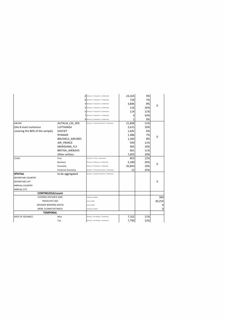
2 Dummy (= 1 if equal to 2, = 0 otherwise) 23,165 9%
3 Dummy (= 1 if equal to 3, = 0 otherwise) 729 7%
4 Dummy (= 1 if equal to 4, = 0 otherwise) 3,846 8%
5 Dummy (= 1 if equal to 5, = 0 otherwise) 114 16%
6 Dummy (= 1 if equal to 6, = 0 otherwise) 114 11%
7 Dummy (= 1 if equal to 7, = 0 otherwise) 3 33%
8 Dummy (= 1 if equal to 8, = 0 otherwise) 1 0%
AIRLINE ALITALIA_CAI_SPA Dummy (= 1 if equal to that level, = 0 otherwise) 21,838 11%
(the 8 most numerous LUFTHANSA 2,615 10%
covering the 80% of the sample) EASYJET 1,642 6%
RYANAIR 1,486 7%
BRUSSELS_AIRLINES 1,260 8%
AIR_FRANCE 939 11%
MERIDIANA_FLY 905 10%
BRITISH_AIRWAYS 601 11%
Other airlines 7,603 10%
CLASS First Dummy (= 1 if First, = 0 otherwise) 853 12%
Business Dummy (= 1 if Business, = 0 otherwise) 2,180 20%
Economy Dummy (= 1 if Economy, = 0 otherwise) 35,843 10%
Premium Economy Dummy (= 1 if Premium Economy, = 0 otherwise) 12 25%
SPATIAL to be aggregated Dummy (= 1 if equal to that level, = 0 otherwise)
DEPARTURE COUNTRY
DEPARTURE CIYY
ARRIVAL COUNTRY
ARRIVAL CITY
continuous variable 300
count variable 30,254
count variable 0
continuous variable 0
DATE OF ISSUANCE Mon Dummy (= 1 for Monday, = 0 otherwise) 7,101 11%
Tue Dummy (= 1 for Tuesday, = 0 otherwise) 7,790 12%
CONTINUOUS/count
COVERED DISTANCE (KM)
TRAVELER'S AGE
ADVANCE BOOKING (DAYS)
(NON_FLOWN DISTANCE)
TEMPORAL
0
0
0
0
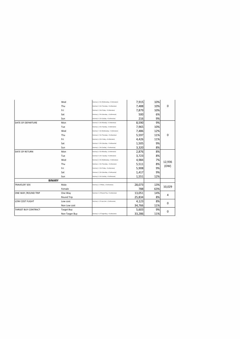
Wed Dummy (= 1 for Wednesday, = 0 otherwise) 7,915 10%
Thu Dummy (= 1 for Thursday, = 0 otherwise) 7,488 10%
Fri Dummy (= 1 for Friday, = 0 otherwise) 7,879 10%
Sat Dummy (= 1 for Saturday, = 0 otherwise) 500 6%
Sun Dummy (= 1 for Sunday, = 0 otherwise) 216 9%
DATE OF DEPARTURE Mon Dummy (= 1 for Monday, = 0 otherwise) 8,590 9%
Tue Dummy (= 1 for Tuesday, = 0 otherwise) 7,965 10%
Wed Dummy (= 1 for Wednesday, = 0 otherwise) 7,486 12%
Thu Dummy (= 1 for Thursday, = 0 otherwise) 5,597 11%
Fri Dummy (= 1 for Friday, = 0 otherwise) 4,426 11%
Sat Dummy (= 1 for Saturday, = 0 otherwise) 1,505 9%
Sun Dummy (= 1 for Sunday, = 0 otherwise) 3,320 8%
DATE OF RETURN Mon Dummy (= 1 for Monday, = 0 otherwise) 2,876 8%
Tue Dummy (= 1 for Tuesday, = 0 otherwise) 3,723 8%
Wed Dummy (= 1 for Wednesday, = 0 otherwise) 4,984 7%
Thu Dummy (= 1 for Thursday, = 0 otherwise) 5,511 8%
Fri Dummy (= 1 for Friday, = 0 otherwise) 5,908 9%
Sat Dummy (= 1 for Saturday, = 0 otherwise) 1,417 9%
Sun Dummy (= 1 for Sunday, = 0 otherwise) 1,551 12%
TRAVELER' SEX Male Dummy (= 1 if Male, = 0 otherwise) 28,073 13%
Female 788 63%
ONE WAY /ROUND TRIP One Way Dummy (= 1 if Round Trip, = 0 otherwise) 13,051 14%
Round Trip 25,834 8%
LOW COST FLIGHT Low cost Dummy (= 1 if Low Cost, = 0 otherwise) 4,123 8%
Non Low cost 34,766 11%
TARGET BUY CONTRACT Target Buy 5,603 9%
Non Targer Buy Dummy (= 1 if Target Buy, = 0 otherwise) 33,286 11%
BINARY
4
0
0
0
0
12,936
(OW)
10,029

3.3#1 51
Though the potential explanatory variables are numerous, it is likely thatsome of them encompass at least part of the information carried by others.In particular:
• some levels of the variable ’professional status’ are observable only incertain type of client companies (e.g. professional status in the armyand magistrate are only observable in public administration);
• the variable ’route’ includes ’departure city’ and ’arrival city’, whichin turn implicitly include ’departure country’ and ’arrival country’ re-spectively. Thus, it partially encompasses also the ’type of air ticket’and ’one way/round trip’;
• the variable ’covered distance’ is strictly related to ’route’, ’number ofroutes’, ’one way/round trip’ and ’type of air ticket’;
• the ’traveler’s age’ can be related to the ’professional status’ of thebusiness traveler;
• if considered jointly, ’date of issuance’ and ’date of departure’ encom-pass the information carried by ’advance booking’, which equals to thenumber of days elapsed between them.
Therefore, it is necessary to choose the best predictor between ’equivalent’variables or to extract common factors from variables encompassing one an-other. The second solution would make results very hardly interpretableand require more complicated elaboration for implementation in the busi-ness activity of the TMC, therefore it is excluded. Next chapter explainshow explanatory variables are chosen, when dealing with the models specifi-cation.

52 3.#1
3.4 Missing data and selection bias
As beckoned above, no missing data is present in automatically collectedvariables, namely:
• output of the ticket,
• date of departure,
• date of issuance,
• advance booking,
• route,
• class,
• whether low cost,
• airline,
• city of departure,
• country of departure,
• city of arrival,
• country of arrival,
• number of routes,
• type of ticket.
While the number and percentage of missing data in each manually collectedcandidate explanatory variable are listed in table 2 below.
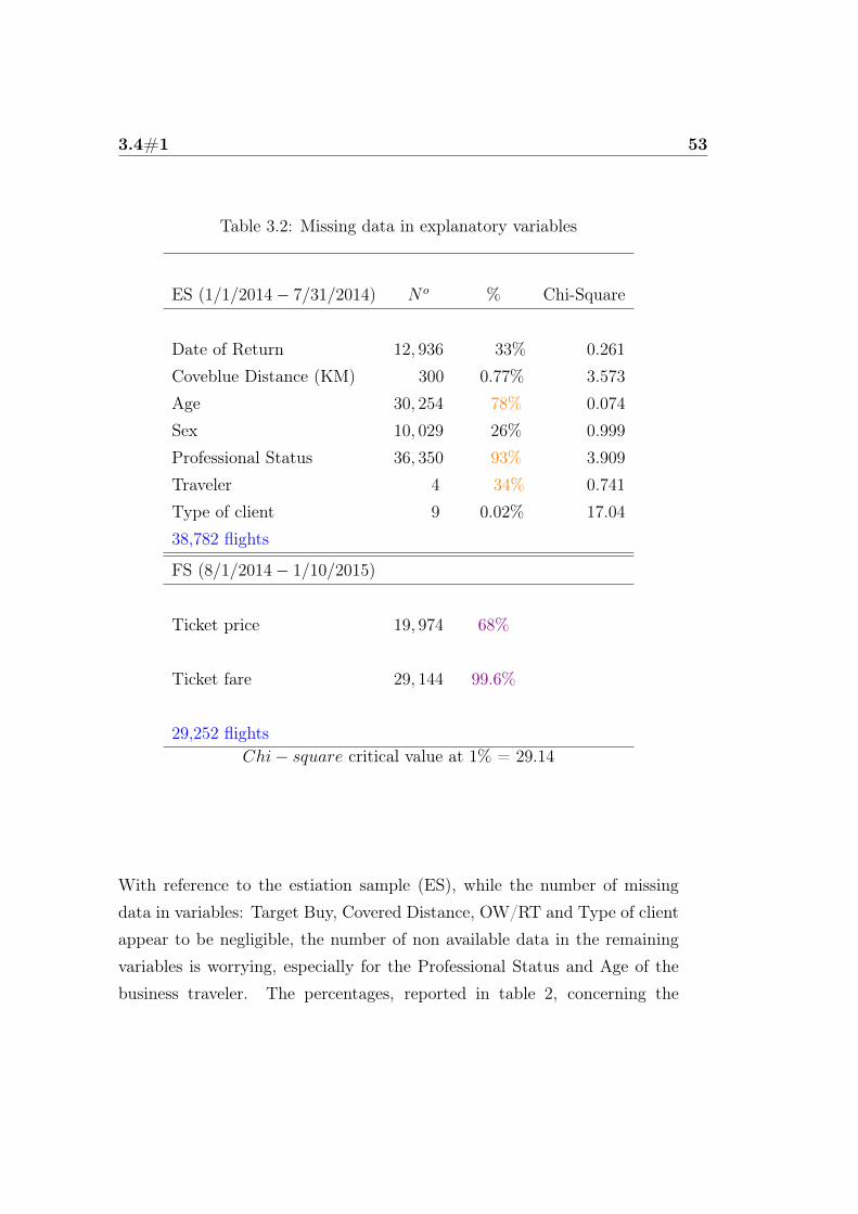
3.4#1 53
Table 3.2: Missing data in explanatory variables
ES (1/1/2014− 7/31/2014) N o % Chi-Square
Date of Return 12, 936 33% 0.261
Coveblue Distance (KM) 300 0.77% 3.573
Age 30, 254 78% 0.074
Sex 10, 029 26% 0.999
Professional Status 36, 350 93% 3.909
Traveler 4 34% 0.741
Type of client 9 0.02% 17.04
38,782 flights
FS (8/1/2014− 1/10/2015)
Ticket price 19, 974 68%
Ticket fare 29, 144 99.6%
29,252 flightsChi− square critical value at 1% = 29.14
With reference to the estiation sample (ES), while the number of missingdata in variables: Target Buy, Covered Distance, OW/RT and Type of clientappear to be negligible, the number of non available data in the remainingvariables is worrying, especially for the Professional Status and Age of thebusiness traveler. The percentages, reported in table 2, concerning the
54 3.#1
latter, suggest to exclude them from the analysis, but theoretically thesevariables should have a great influence on the probability of non-departure.
In fact, it can be hypothesized that the lower the professional statusof the traveler, in his company’s hierarchy, the lower the probability that hecan postpone or avoid a journey, which is likely to have been imposed by hisboss, and vice versa. Moreover, it may be that the age of the traveler canapproximate his professional status, as it seems probable that the older theworker, the more career he did, the higher his status in the hierarchy, thehigher the probability that he can waive or change the journey. The numberof observed tickets for which the information on both the professional statusand the age are missing is 28,602 (the 73%).
Therefore, in order to verify if it is meaningful to perform a separatevariables selection (see next chapter), including only rows for which theseappearently importan variables are observed, it is useful to look at thechi-squared test on the differences in relative frequencies of the dependentvariable, between missing and non-missing data in exogenous variables, todetect the presence of selection bias (as e.g. in: Berger and Exner, 1999;McNichols and O’Brien, 1997) .The values of chi-squared statistics, reported in table 2, allow to acceptthe null hypothesis of no selection bias for all of the variables, with aP-value lower than 1%. Thus, these variables can be used to calculate theconditional probability of non-flights, at least for tickets for which theyare observed. But, to avoid favoring the significance of variables with lessmissing data (allowing to estimate models with more degrees of freedom), aseparate selection on complete observations it is made.
As previously mentioned, most of the data are automatically collectedby the IT system of the TMC since the 1st January 2014, but some dataon the two previous years were manually inserted in the database. Thus, itis possible to visualize a relatively long historical dynamic of Yf , based oneither the date of issuance of the air ticket, or that of departure, or that
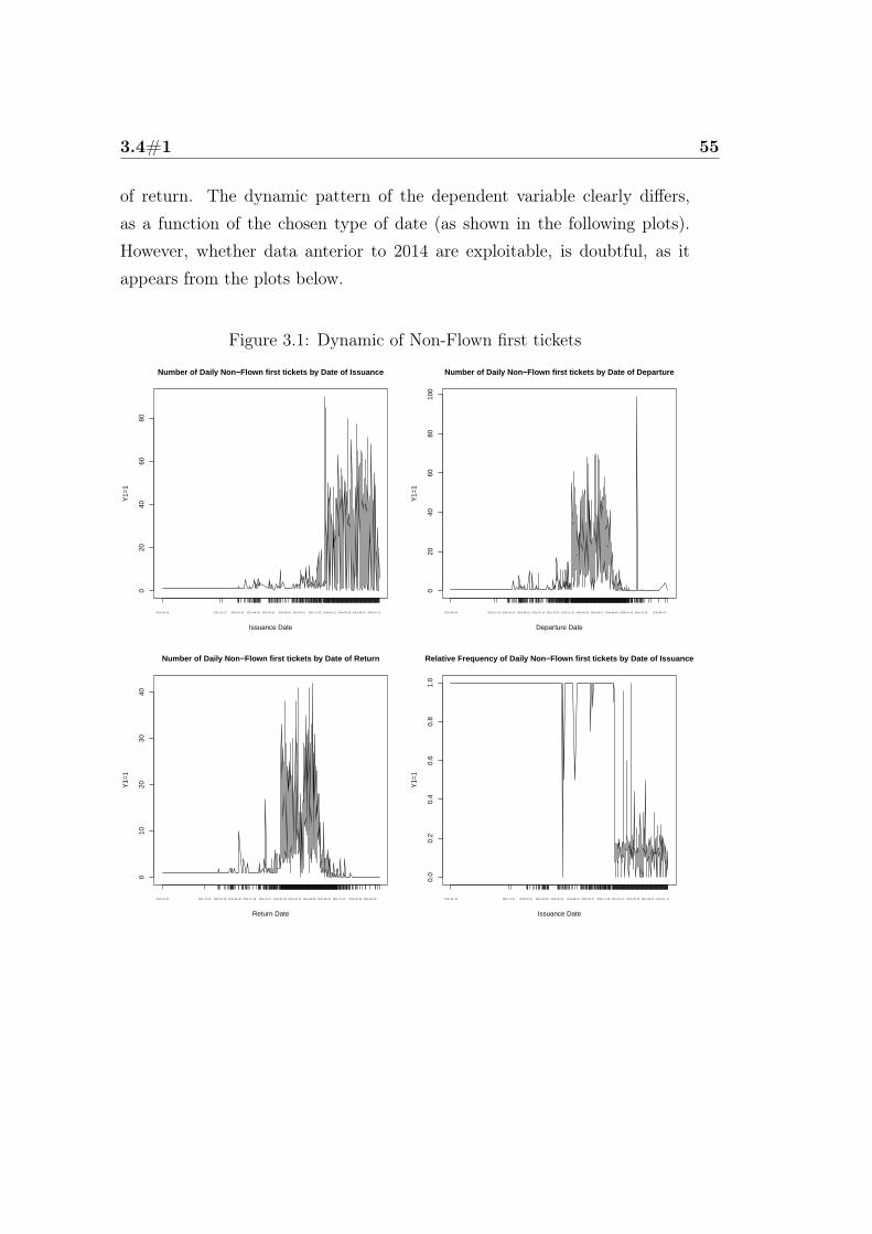
3.4#1 55
of return. The dynamic pattern of the dependent variable clearly differs,as a function of the chosen type of date (as shown in the following plots).However, whether data anterior to 2014 are exploitable, is doubtful, as itappears from the plots below.
Figure 3.1: Dynamic of Non-Flown first tickets
020
4060
80
Number of Daily Non−Flown first tickets by Date of Issuance
Issuance Date
Y1=
1
2012−04−18 2012−11−27 2013−02−01 2013−04−03 2013−05−31 2013−08−01 2013−09−27 2013−11−25 2014−01−21 2014−03−19 2014−05−15 2014−07−11
020
4060
8010
0
Number of Daily Non−Flown first tickets by Date of Departure
Departure Date
Y1=
1
2012−04−20 2012−11−29 2013−02−13 2013−05−01 2013−07−16 2013−10−01 2013−12−16 2014−03−02 2014−05−17 2014−08−01 2014−10−16 2014−12−31 2015−04−03
010
2030
40
Number of Daily Non−Flown first tickets by Date of Return
Return Date
Y1=
1
2012−04−20 2012−12−01 2013−02−19 2013−05−09 2013−07−26 2013−10−17 2014−01−03 2014−03−22 2014−06−08 2014−08−25 2014−11−12 2015−02−06 2015−04−25
0.0
0.2
0.4
0.6
0.8
1.0
Relative Frequency of Daily Non−Flown first tickets by Date of Issuance
Issuance Date
Y1=
1
2012−04−18 2012−11−27 2013−02−01 2013−04−03 2013−05−31 2013−08−01 2013−09−27 2013−11−25 2014−01−21 2014−03−19 2014−05−15 2014−07−11
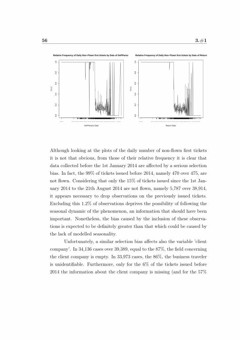
56 3.#1
0.0
0.2
0.4
0.6
0.8
1.0
Relative Frequency of Daily Non−Flown first tickets by Date of DePParture
DePParture Date
Y1=
1
2012−04−20 2012−11−29 2013−02−13 2013−05−01 2013−07−16 2013−10−01 2013−12−16 2014−03−02 2014−05−17 2014−08−01 2014−10−16 2014−12−31 2015−04−03
0.0
0.2
0.4
0.6
0.8
1.0
Relative Frequency of Daily Non−Flown first tickets by Date of Return
Return Date
Y1=
1
2012−04−20 2012−12−01 2013−02−19 2013−05−09 2013−07−26 2013−10−17 2014−01−03 2014−03−22 2014−06−08 2014−08−25 2014−11−12 2015−02−06 2015−04−25
Although looking at the plots of the daily number of non-flown first ticketsit is not that obvious, from those of their relative frequency it is clear thatdata collected before the 1st January 2014 are affected by a serious selectionbias. In fact, the 99% of tickets issued before 2014, namely 470 over 475, arenot flown. Considering that only the 15% of tickets issued since the 1st Jan-uary 2014 to the 21th August 2014 are not flown, namely 5,787 over 38,914,it appears necessary to drop observations on the previously issued tickets.Excluding this 1.2% of observations deprives the possibility of following theseasonal dynamic of the phenomenon, an information that should have beenimportant. Nonetheless, the bias caused by the inclusion of these observa-tions is expected to be definitely greater than that which could be caused bythe lack of modelled seasonality.
Unfortunately, a similar selection bias affects also the variable ’clientcompany’. In 34,136 cases over 39,389, equal to the 87%, the field concerningthe client company is empty. In 33,973 cases, the 86%, the business traveleris unidentifiable. Furthermore, only for the 6% of the tickets issued before2014 the information about the client company is missing (and for the 57%
3.4#1 57
of the tickets issued in 2014). Of the remaining 94%, the 99% are not flown.While, in the whole database, 5,006 first tickets over 5,253, for which theclient company is known, equal to the 95% are not flown. Limiting the cal-culus to 2014, this percentage stays at 95%. Only the 4% of tickets issuedbefore 2014 miss the identification of the corresponing business traveler. Ofthe remaining 96%, the 71% are not flown.
These percentages suggest that a separate analysis should be con-ducted for tickets for which the client company is identifiable. Thus, a furthervariables selection is performed only on observations complete with referenceto this information, using variables descrribing the past behavior of the com-pany and the business traveler. The first are intended to be indicators of thecompany’s business, stage of development, economic condition and interna-tionalization degree. The second is meant to be a proxy for the traveler’sprivate life, family situation and professional role.
Among these ’past−behavior’ variables, only a few resulted significant(see next chapter) and are reported here:
• NflightsC: number of flights purchased by the company (during theperiod spanned by the estimation sample).
• OccTravC: dummy variable, equal to 1 if the company requres businessflights rarely (with a frequency less than the tird quartile), 0 otherwise.
• OccCh: dummy variable, equal to 1 if the traveler changed ticketsrarely (with a frequency less than the tird quartile), 0 otherwise.
• OccTrav: dummy variable, equal to 1 if the worker flies rarely (with afrequency less than the tird quartile), 0 otherwise.
• AverTrav: : dummy variable, equal to 1 if the frequency of flights,booked in the name of the traveler, is included in the second or tirdquartile), 0 otherwise.
58 3.#1
• FreqWai: dummy variable, equal to 1 if the traveler cancels the flightoften (with a frequency included in the first quartile), 0 otherwise.
Indeed, variables OccCh and FreqWai are tautological for descriptive pur-poses, but crucial in prediction, as shown in the final chapter.
With reference to the forecasting sample (FS in table 1.2), the toomany missing data about the cost of tickets and their fare make impossi-ble to estimate the expected cost of flights, to provide an actual (not basedon approximation) economic evaluation of the predictors’ performance andrequires the development of a different method to assess the economic per-formance of what will be the proposed solution.
3.5 Descriptive statistics
Once removed data collected prior to 2014 and those presenting mis-takes, the sample includes 38,782 observations. The sample temporaldistribution of air tickets purchases can be viewed as a function of thedate of issuance, date of departure and date of return. It is shown in figure 2.
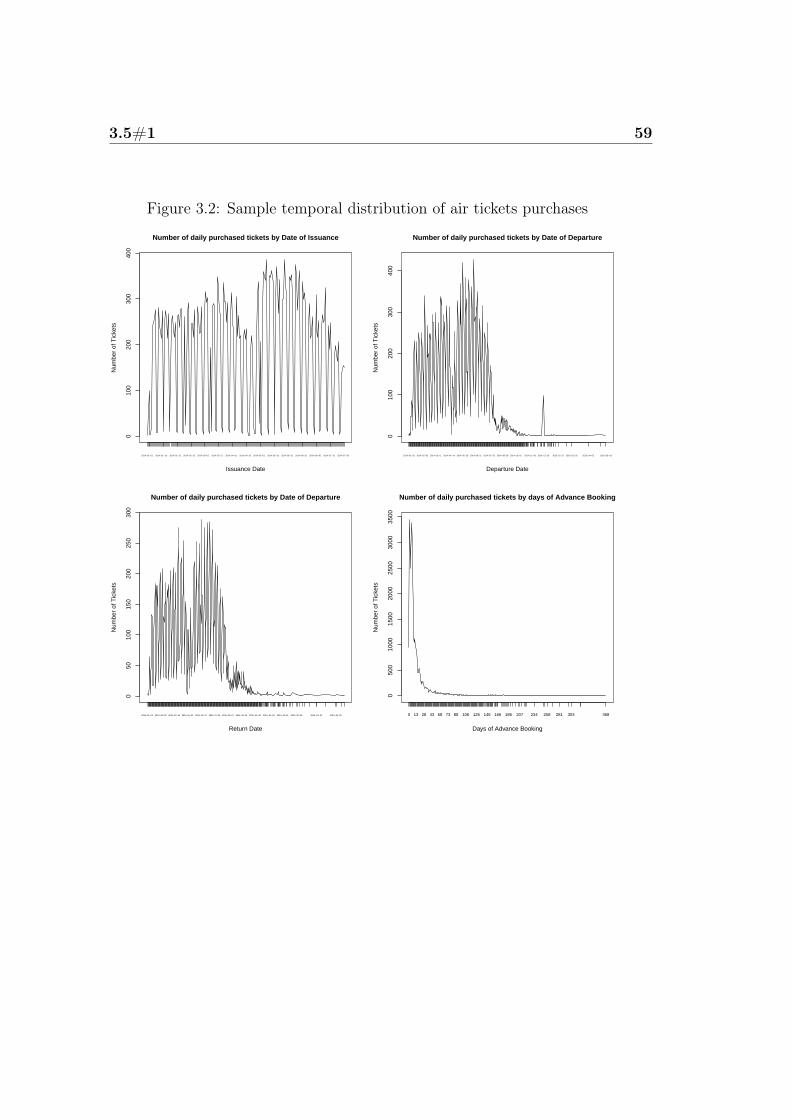
3.5#1 59
Figure 3.2: Sample temporal distribution of air tickets purchases
010
020
030
040
0
Number of daily purchased tickets by Date of Issuance
Issuance Date
Num
ber
of T
icke
ts
2014−01−01 2014−01−16 2014−01−31 2014−02−15 2014−03−02 2014−03−17 2014−04−01 2014−04−16 2014−05−01 2014−05−16 2014−05−31 2014−06−15 2014−06−30 2014−07−15 2014−07−30
010
020
030
040
0
Number of daily purchased tickets by Date of Departure
Departure Date
Num
ber
of T
icke
ts
2014−01−02 2014−02−05 2014−03−11 2014−04−14 2014−05−18 2014−06−21 2014−07−25 2014−08−28 2014−10−01 2014−11−06 2014−12−10 2015−01−17 2015−02−20 2015−04−03 2015−05−18
050
100
150
200
250
300
Number of daily purchased tickets by Date of Departure
Return Date
Num
ber
of T
icke
ts
2014−01−03 2014−02−08 2014−03−16 2014−04−21 2014−05−27 2014−07−02 2014−08−07 2014−09−12 2014−10−18 2014−11−24 2014−12−31 2015−02−06 2015−03−31 2015−05−22
050
010
0015
0020
0025
0030
0035
00
Number of daily purchased tickets by days of Advance Booking
Days of Advance Booking
Num
ber
of T
icke
ts
0 13 28 43 58 73 88 106 126 146 166 186 207 234 258 281 303 368
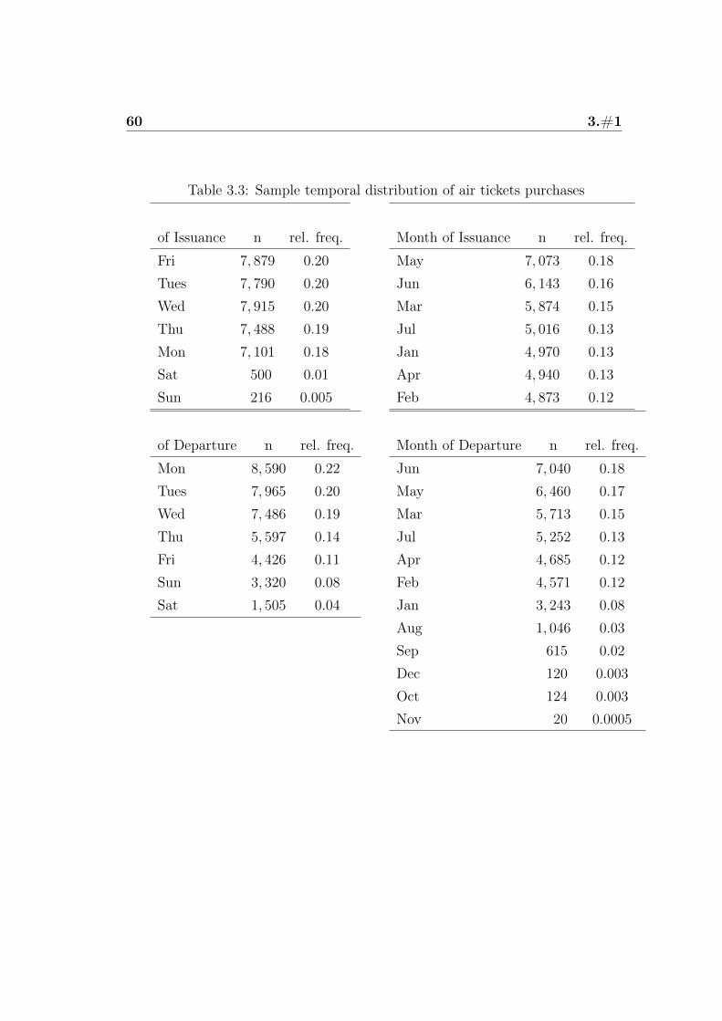
60 3.#1
Table 3.3: Sample temporal distribution of air tickets purchases
of Issuance n rel. freq.
Fri 7, 879 0.20
Tues 7, 790 0.20
Wed 7, 915 0.20
Thu 7, 488 0.19
Mon 7, 101 0.18
Sat 500 0.01
Sun 216 0.005
Month of Issuance n rel. freq.
May 7, 073 0.18
Jun 6, 143 0.16
Mar 5, 874 0.15
Jul 5, 016 0.13
Jan 4, 970 0.13
Apr 4, 940 0.13
Feb 4, 873 0.12
of Departure n rel. freq.
Mon 8, 590 0.22
Tues 7, 965 0.20
Wed 7, 486 0.19
Thu 5, 597 0.14
Fri 4, 426 0.11
Sun 3, 320 0.08
Sat 1, 505 0.04
Month of Departure n rel. freq.
Jun 7, 040 0.18
May 6, 460 0.17
Mar 5, 713 0.15
Jul 5, 252 0.13
Apr 4, 685 0.12
Feb 4, 571 0.12
Jan 3, 243 0.08
Aug 1, 046 0.03
Sep 615 0.02
Dec 120 0.003
Oct 124 0.003
Nov 20 0.0005
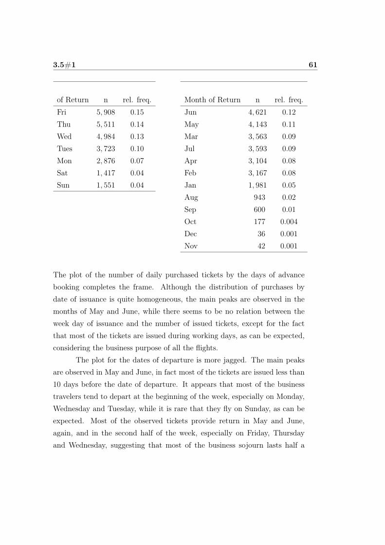
3.5#1 61
of Return n rel. freq.
Fri 5, 908 0.15
Thu 5, 511 0.14
Wed 4, 984 0.13
Tues 3, 723 0.10
Mon 2, 876 0.07
Sat 1, 417 0.04
Sun 1, 551 0.04
Month of Return n rel. freq.
Jun 4, 621 0.12
May 4, 143 0.11
Mar 3, 563 0.09
Jul 3, 593 0.09
Apr 3, 104 0.08
Feb 3, 167 0.08
Jan 1, 981 0.05
Aug 943 0.02
Sep 600 0.01
Oct 177 0.004
Dec 36 0.001
Nov 42 0.001
The plot of the number of daily purchased tickets by the days of advancebooking completes the frame. Although the distribution of purchases bydate of issuance is quite homogeneous, the main peaks are observed in themonths of May and June, while there seems to be no relation between theweek day of issuance and the number of issued tickets, except for the factthat most of the tickets are issued during working days, as can be expected,considering the business purpose of all the flights.
The plot for the dates of departure is more jagged. The main peaksare observed in May and June, in fact most of the tickets are issued less than10 days before the date of departure. It appears that most of the businesstravelers tend to depart at the beginning of the week, especially on Monday,Wednesday and Tuesday, while it is rare that they fly on Sunday, as can beexpected. Most of the observed tickets provide return in May and June,again, and in the second half of the week, especially on Friday, Thursdayand Wednesday, suggesting that most of the business sojourn lasts half a

62 3.#1
week. While it is rare that travelers come back on Saturday.The spatial distribution of the sample, by country of departure and
country of arrival is shown in figure 3.

3.5#1 63
Figure 3.3: Sample spacial distribution of air tickets purchases
ALBANIA ARUBA BAHRAIN BRAZIL CAMEROON CHINA COTE_D'IVOIRE DENMARK ESTONIA GABON GHANA ICELAND IRAN IRAQ ITALIA JORDAN KUWAIT LITHUANIA MALDIVES MEXICO MOZAMBIQUE NIGERIA POLAND RUSSIA SIERRA_LEONE SPAIN THAILAND UGANDA URUGUAY YUGOSLAVIA
050
0010
000
1500
020
000
2500
030
000
Aberdeen Amman Athens Bangalore Beijing Billund Boston Brussels Cairo Chania Cork Delhi Dubai Entebbe Genoa Guernsey Heraklion Istanbul Kayseri Kosice Larnaca Linz Lugano Malta Medellin Minsk Munich Newark Odessa Paris Pisa Prague Reykjavik Salzburg Sanya Shiraz Stockholm Tashkent Tokyo Tunis Vienna Wroclaw Zurich
020
0040
0060
0080
0010
000
1200
0
ALBANIA AUSTRALIA BELARUS BRAZIL CAMBODIA CHILE CONGO CUBA DJIBOUTI EGYPT FINLAND GEORGIA GUINEA INDIA IRAQ ITALY JORDAN KUWAIT LITHUANIA MALDIVES MEXICO MYANMAR NIGERIA PANAMA POLAND RUSSIA SINGAPORE SWEDEN THAILAND UGANDA URUGUAY ZAMBIA
050
0010
000
1500
020
000
Aalborg Alghero Ankara Athens Bangkok Belfast Bishkek Brest Cagliari Catania Cluj Cork Doha Durban FORLI Goa Hanoi Houston Izmir Kavala Kosice Lagos Leon LUBLIN Male Medellin Minsk Muscat Niamey Olbia Pamplona Perth Pisa Prague Quito Riga Salzburg Sanya Simferopol Stuttgart Tenerife Trieste VAN Vigo Wroclaw
020
0040
0060
00
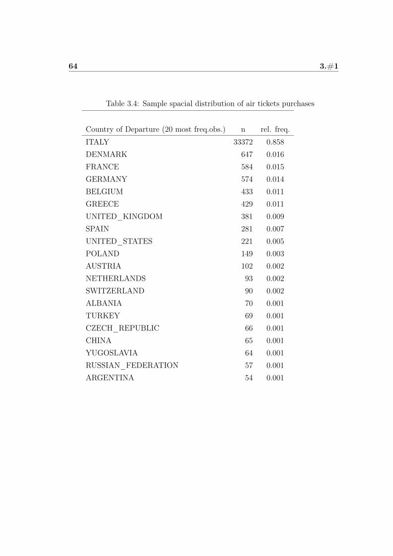
64 3.#1
Table 3.4: Sample spacial distribution of air tickets purchases
Country of Departure (20 most freq.obs.) n rel. freq.
ITALY 33372 0.858
DENMARK 647 0.016
FRANCE 584 0.015
GERMANY 574 0.014
BELGIUM 433 0.011
GREECE 429 0.011
UNITED_KINGDOM 381 0.009
SPAIN 281 0.007
UNITED_STATES 221 0.005
POLAND 149 0.003
AUSTRIA 102 0.002
NETHERLANDS 93 0.002
SWITZERLAND 90 0.002
ALBANIA 70 0.001
TURKEY 69 0.001
CZECH_REPUBLIC 66 0.001
CHINA 65 0.001
YUGOSLAVIA 64 0.001
RUSSIAN_FEDERATION 57 0.001
ARGENTINA 54 0.001

3.5#1 65
City of Departure (20 most freq. obs.) n rel. freq.
Rome 12419 0.319
Milan 8956 0.23
Turin 1666 0.0428
Palermo 1311 0.0337
Naples 1134 0.0292
Catania 1078 0.0277
Cagliari 973 0.025
Bari 958 0.0246
Genoa 835 0.0215
Venice 675 0.0174
Copenhagen 645 0.0166
Paris 467 0.012
Brussels 432 0.0111
Florence 428 0.011
Brindisi 425 0.0109
Bologna 417 0.0107
Trieste 375 0.0096
Lamezia_Terme 340 0.0087
Frankfurt 305 0.0078
Athens 291 0.0074
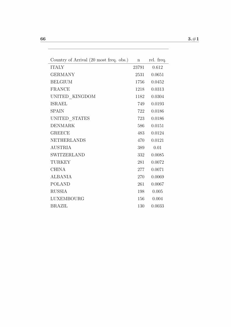
66 3.#1
Country of Arrival (20 most freq. obs.) n rel. freq.
ITALY 23791 0.612
GERMANY 2531 0.0651
BELGIUM 1756 0.0452
FRANCE 1218 0.0313
UNITED_KINGDOM 1182 0.0304
ISRAEL 749 0.0193
SPAIN 722 0.0186
UNITED_STATES 723 0.0186
DENMARK 586 0.0151
GREECE 483 0.0124
NETHERLANDS 470 0.0121
AUSTRIA 389 0.01
SWITZERLAND 332 0.0085
TURKEY 281 0.0072
CHINA 277 0.0071
ALBANIA 270 0.0069
POLAND 261 0.0067
RUSSIA 198 0.005
LUXEMBOURG 156 0.004
BRAZIL 130 0.0033

3.5#1 67
City of Arrival (20 most freq. obs.) n rel. freq.
Rome 7977 0.205
Milan 5874 0.151
Brussels 1754 0.0451
Frankfurt 1627 0.0418
Naples 1214 0.0312
Palermo 1201 0.0309
Paris 1022 0.0263
London 967 0.0249
Catania 906 0.0233
Bari 860 0.0221
Tel_Aviv_Yafo 749 0.0193
Cagliari 743 0.0191
Turin 731 0.0188
Genoa 724 0.0186
Copenhagen 575 0.0148
Venice 526 0.0135
Amsterdam 456 0.0117
Brindisi 447 0.0115
Lamezia_Terme 384 0.0098
Vienna 383 0.0098
As in one way tickets the arrival city/country for the way-forward equalsthe departure city/country for the way-back, considering that Seneca islocated in Italy, thus many of its clients have headquarters in Italy, it isnot surprising that Italy and italian cities are the most observed locations.Table 5 shows only places observed at least 4 times, the complete table isavailable upon request.
Table 6 shows the composition of the sample by route.

68 3.#1
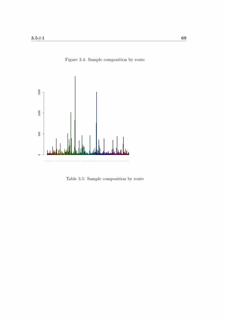
3.5#1 69
Figure 3.4: Sample composition by route
ABJ_CMN_TRN_CMN_ABJ AEP_FCO AHO_CIA AHO_LIN ALC_BCN_CPH ALC_MUC AMM_BAH AMS_BLQ AMS_HER AMS_MAN AMS_PRG AMS_ZRH AOI_FCO_REG ARN_AMS ARN_MAD_ARN ATH_ADB_ATH ATH_BRU ATH_BUD ATH_FCO ATH_FRA ATH_HER ATH_KVA ATH_MUC_CPH ATH_VCE ATH_ZRH ATL_MIA BAH_KWI BCN_BLQ
050
010
0015
00
Table 3.5: Sample composition by route

70 3.#1
Route (20 most freq. obs.) n rel. freq.
FCO/LIN/FCO 1884 0.0664
LIN/FCO/LIN 1507 0.0531
FCO/FRA/FCO 1022 0.036
FCO/LIN 836 0.0294
LIN/FCO 760 0.0268
FCO/BRU/FCO 515 0.0181
FCO/TLV/FCO 463 0.0163
GOA/FCO/GOA 463 0.0163
PMO/FCO/PMO 448 0.0158
TRN/FCO/TRN 431 0.0152
FCO/GOA/FCO 397 0.014
CAG/FCO/CAG 392 0.0138
MXP/BRU/MXP 389 0.0137
FCO/CDG/FCO 373 0.0131
LIN/NAP 366 0.0129
NAP/LIN 358 0.0126
FCO/PMO/FCO 341 0.012
CTA/FCO/CTA 273 0.0096
TRN/FCO 263 0.0092
FCO/TRN/FCO 243 0.0085
The variable ’route’ is more heterogeneous than the variables of places ofdeparture and arrival, because the same destination can be reached throughdifferent routes, from the same departure city, but also because of ’crossedtickets’. The above tables show only the 20 most frequently observed routesor places, to save space. The full tables are available upon request.
More synthetic variables, describing a characteristics of the path be-tween the city of departure and that of arrival, are constituted by the number
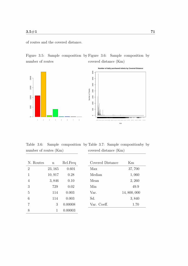
3.5#1 71
of routes and the covered distance.
Figure 3.5: Sample composition bynumber of routes
1 2 3 4 5 6 7 8
050
0010
000
1500
020
000
Figure 3.6: Sample composition bycovered distance (Km)
050
010
0015
0020
0025
0030
0035
00
Number of daily purchased tickets by Covered Distance
Km
Num
ber
of T
icke
ts
49.88966 2230.55078 4628.47334 7029.61459 9454.89600 11996.05018 14612.84352 17232.85555 19859.30496 22485.75437 25179.79622 28330.89178 31456.23782 34340.18227 37677.96173
Table 3.6: Sample composition bynumber of routes (Km)
N. Routes n Rel.Freq
2 23, 165 0.601
1 10, 917 0.28
4 3, 846 0.10
3 729 0.02
5 114 0.003
6 114 0.003
7 3 0.00008
8 1 0.00003
Table 3.7: Sample compositionby bycovered distance (Km)
Covered Distance Km
Max 37, 700
Median 1, 060
Mean 2, 260
Min 49.9
Var. 14, 800, 000
Sd. 3, 840
Var. Coeff. 1.70

72 3.#1
Most of the observed flights include an only stopover, flights including morethan 4 stopovers are very few, possibly related to ’crossed tickets’. Most ofthe flights cover a distance shorter than 5,000 Km. The 4 outstanding peaksin figure 6 correspond to flights covering: 940 Km, 470 Km, 1,918 Km and798 Km of distance, in decreasing order of relative frequency.
Consistently with the fact that most of the flights depart from andarrive in an Italian city, most of the observed air tickets are national. Roundtrip itineraries are nearly the double of one-way ones, that can be explainedby the lower cost of the first ones, ceteris paribus. These informations areshown in figures 5 and 6.
Figure 3.7: Sample composition byticket type
Intercontinental International National
050
0010
000
1500
020
000
Figure 3.8: Sample composition bytype of itinerary
OW RT
050
0010
000
1500
020
000
2500
0

3.5#1 73
Table 3.8: Sample composition byticket type
Type of ticket n Rel.Freq
Intercont 3, 603 0.093
Internat 1, 4013 0.360
National 21, 273 0.547
Table 3.9: Sample composition bytype of itinerary
Type of itinerary n Rel.Freq
OW 13051 0.336
RT 25834 0.664
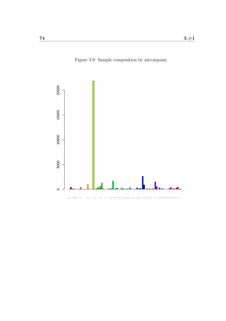
74 3.#1
Figure 3.9: Sample composition by aircompany
AEROMEXICO GERMANWINGS WESTJET TRANSAVIA ICELANDAIR AIR_MALTA JET2 US_AIRWAYS AIR_CHINA AIR_DOLOMITI FLYBE CROATIA_AIRLINES WIZZ_AIR CATHAY_PACIFIC TUNISAIR DELTA_AIR_LINES VOLOTEA AUSTRIAN_AIRLINES VUELING_AIRLINES AIR_FRANCE EASYJET
050
0010
000
1500
020
000
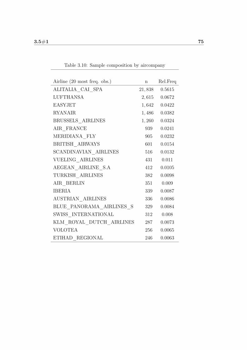
3.5#1 75
Table 3.10: Sample composition by aircompany
Airline (20 most freq. obs.) n Rel.Freq
ALITALIA_CAI_SPA 21, 838 0.5615
LUFTHANSA 2, 615 0.0672
EASYJET 1, 642 0.0422
RYANAIR 1, 486 0.0382
BRUSSELS_AIRLINES 1, 260 0.0324
AIR_FRANCE 939 0.0241
MERIDIANA_FLY 905 0.0232
BRITISH_AIRWAYS 601 0.0154
SCANDINAVIAN_AIRLINES 516 0.0132
VUELING_AIRLINES 431 0.011
AEGEAN_AIRLINE_S.A 412 0.0105
TURKISH_AIRLINES 382 0.0098
AIR_BERLIN 351 0.009
IBERIA 339 0.0087
AUSTRIAN_AIRLINES 336 0.0086
BLUE_PANORAMA_AIRLINES_S 329 0.0084
SWISS_INTERNATIONAL 312 0.008
KLM_ROYAL_DUTCH_AIRLINES 287 0.0073
VOLOTEA 256 0.0065
ETIHAD_REGIONAL 246 0.0063

76 3.#1
Figure 3.10: Sample composition byLow Cost flights
Non LowCost
050
0010
000
1500
020
000
2500
030
000
Table 3.11: Sample composition byLow Cost flights
n Rel.Freq
Non-low cost 34, 766 0.894
Low Cost 4, 123 0.106
Figure 3.11: Sample composition byclass
Business Economy First PremiumEconomy
050
0010
000
1500
020
000
2500
030
000
3500
0
Table 3.12: Sample composition byclass
on-board class n Rel.Freq
Economy 35, 843 0.92
Business 2, 180 0.06
First 853 0.02
PremiumEconomy 12 0.0003
Most of the observed client companies appear to have aimed at savingmoney, though not through low cost flights, but reserving a seat in economyclass (possibly no low cost flight was available for the desired route). Tickets
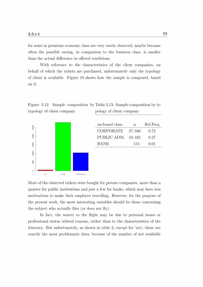
3.5#1 77
for seats in premium economy class are very rarely observed, maybe becauseoften the possible saving, in comparison to the business class, is smallerthan the actual difference in offered conditions.
With reference to the characteristics of the client companies, onbehalf of which the tickets are purchased, unfortunately only the typologyof client is available. Figure 10 shows how the sample is composed, basedon it.
Figure 3.12: Sample composition bytypology of client company
Bank Corporate PublicAdministration
050
0010
000
1500
020
000
2500
0
Table 3.13: Sample composition by ty-pology of client company
on-board class n Rel.Freq
CORPORATE 27, 940 0.72
PUBLIC ADM. 10, 425 0.27
BANK 515 0.01
Most of the observed tickets were bought for private companies, more than aquarter for public institutions and just a few for banks, which may have lessmotivations to make their employee travelling. However, for the purpose ofthe present work, the most interesting variables should be those concerningthe subject who actually flies (or does not fly).
In fact, the waiver to the flight may be due to personal issues orprofessional status related reasons, rather than to the characteristics of theitinerary. But unfortunately, as shown in table 2, except for ’sex’, these areexactly the most problematic data, because of the number of not available
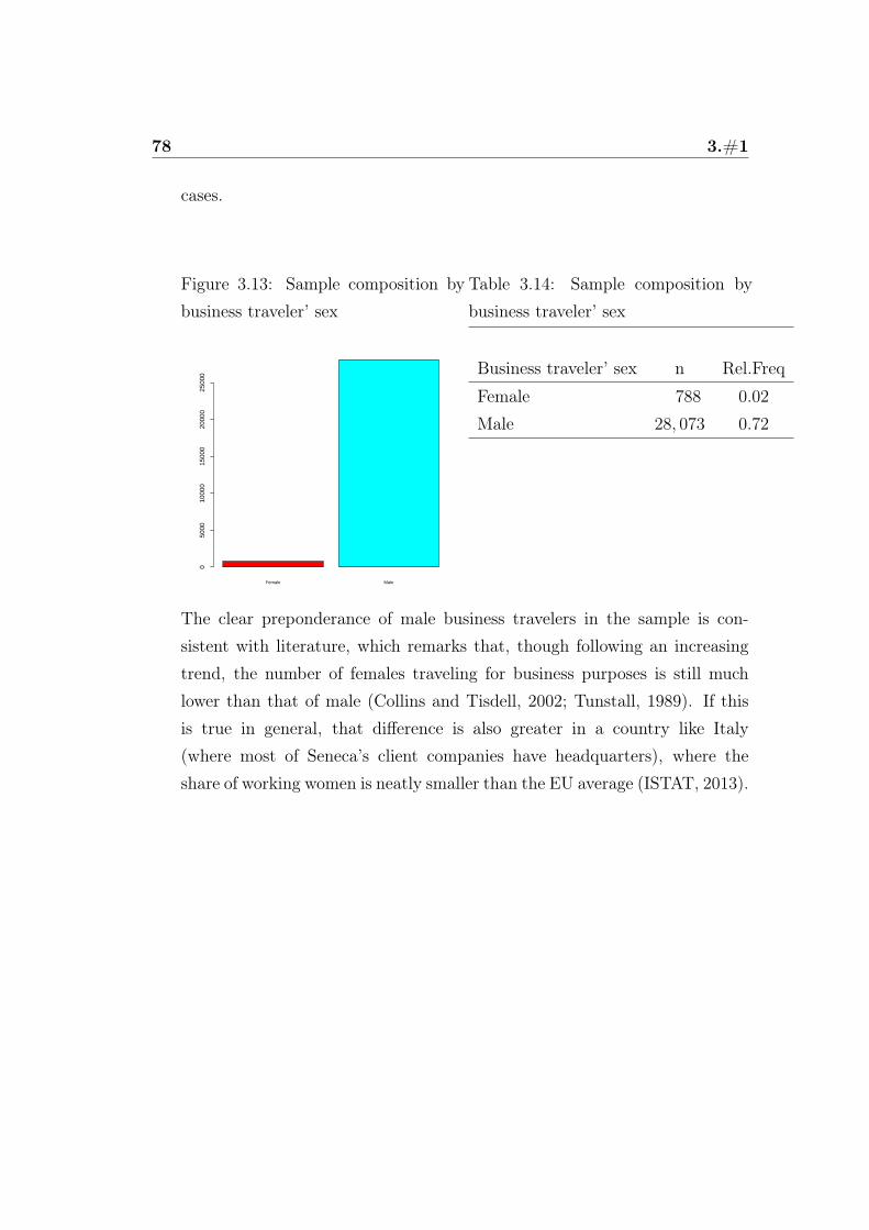
78 3.#1
cases.
Figure 3.13: Sample composition bybusiness traveler’ sex
Female Male
050
0010
000
1500
020
000
2500
0
Table 3.14: Sample composition bybusiness traveler’ sex
Business traveler’ sex n Rel.Freq
Female 788 0.02
Male 28, 073 0.72
The clear preponderance of male business travelers in the sample is con-sistent with literature, which remarks that, though following an increasingtrend, the number of females traveling for business purposes is still muchlower than that of male (Collins and Tisdell, 2002; Tunstall, 1989). If thisis true in general, that difference is also greater in a country like Italy(where most of Seneca’s client companies have headquarters), where theshare of working women is neatly smaller than the EU average (ISTAT, 2013).
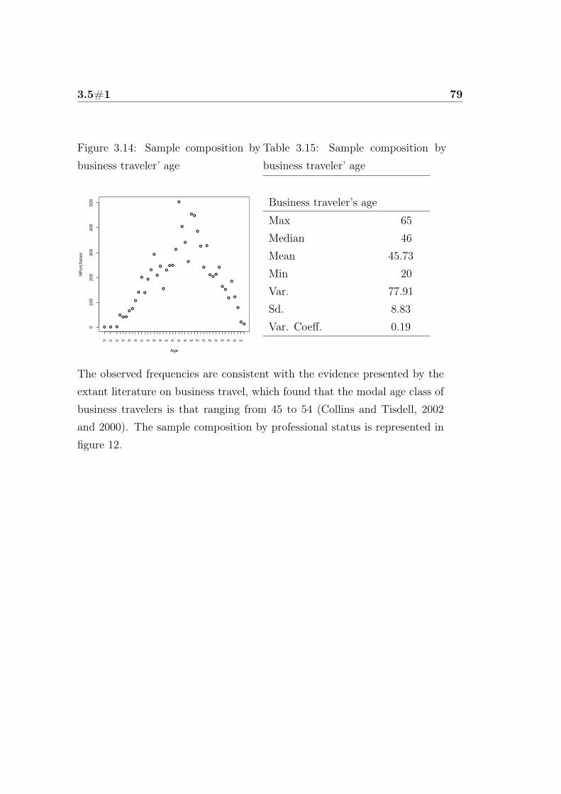
3.5#1 79
Figure 3.14: Sample composition bybusiness traveler’ age
010
020
030
040
050
0
Age
NP
urch
ases
20 22 24 26 28 30 32 34 36 38 40 42 44 46 48 50 52 54 56 58 60 62 64
Table 3.15: Sample composition bybusiness traveler’ age
Business traveler’s age
Max 65
Median 46
Mean 45.73
Min 20
Var. 77.91
Sd. 8.83
Var. Coeff. 0.19
The observed frequencies are consistent with the evidence presented by theextant literature on business travel, which found that the modal age class ofbusiness travelers is that ranging from 45 to 54 (Collins and Tisdell, 2002and 2000). The sample composition by professional status is represented infigure 12.
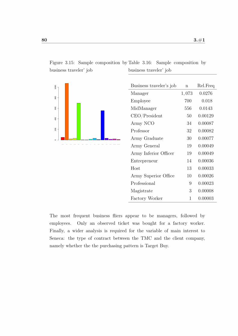
80 3.#1
Figure 3.15: Sample composition bybusiness traveler’ job
CEO/President Manager Army General Army Graduate Employee Magistrate Factory Worker Host Professor Professional MidManager Army NCO Entrepreneur Army Inferior Officer Army Superior Office
020
040
060
080
010
00
Table 3.16: Sample composition bybusiness traveler’ job
Business traveler’s job n Rel.Freq
Manager 1, 073 0.0276
Employee 700 0.018
MidManager 556 0.0143
CEO/President 50 0.00129
Army NCO 34 0.00087
Professor 32 0.00082
Army Graduate 30 0.00077
Army General 19 0.00049
Army Inferior Officer 19 0.00049
Entrepreneur 14 0.00036
Host 13 0.00033
Army Superior Office 10 0.00026
Professional 9 0.00023
Magistrate 3 0.00008
Factory Worker 1 0.00003
The most frequent business fliers appear to be managers, followed byemployees. Only an observed ticket was bought for a factory worker.Finally, a wider analysis is required for the variable of main interest toSeneca: the type of contract between the TMC and the client company,namely whether the the purchasing pattern is Target Buy.
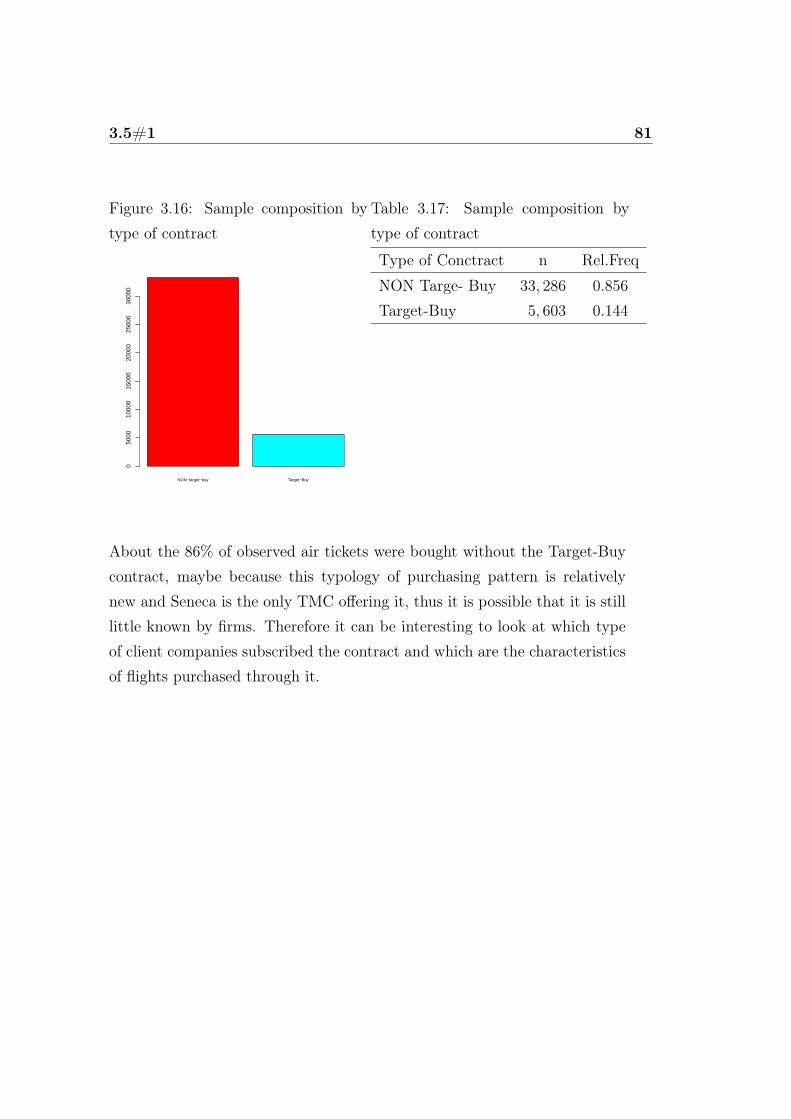
3.5#1 81
Figure 3.16: Sample composition bytype of contract
NON−target−buy Target−Buy
050
0010
000
1500
020
000
2500
030
000
Table 3.17: Sample composition bytype of contract
Type of Conctract n Rel.Freq
NON Targe- Buy 33, 286 0.856
Target-Buy 5, 603 0.144
About the 86% of observed air tickets were bought without the Target-Buycontract, maybe because this typology of purchasing pattern is relativelynew and Seneca is the only TMC offering it, thus it is possible that it is stilllittle known by firms. Therefore it can be interesting to look at which typeof client companies subscribed the contract and which are the characteristicsof flights purchased through it.
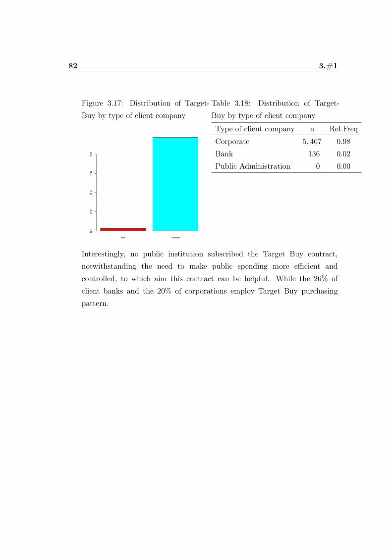
82 3.#1
Figure 3.17: Distribution of Target-Buy by type of client company
Bank Corporate
0.0
0.2
0.4
0.6
0.8
Table 3.18: Distribution of Target-Buy by type of client company
Type of client company n Rel.Freq
Corporate 5, 467 0.98
Bank 136 0.02
Public Administration 0 0.00
Interestingly, no public institution subscribed the Target Buy contract,notwithstanding the need to make public spending more efficient andcontrolled, to which aim this contract can be helpful. While the 26% ofclient banks and the 20% of corporations employ Target Buy purchasingpattern.
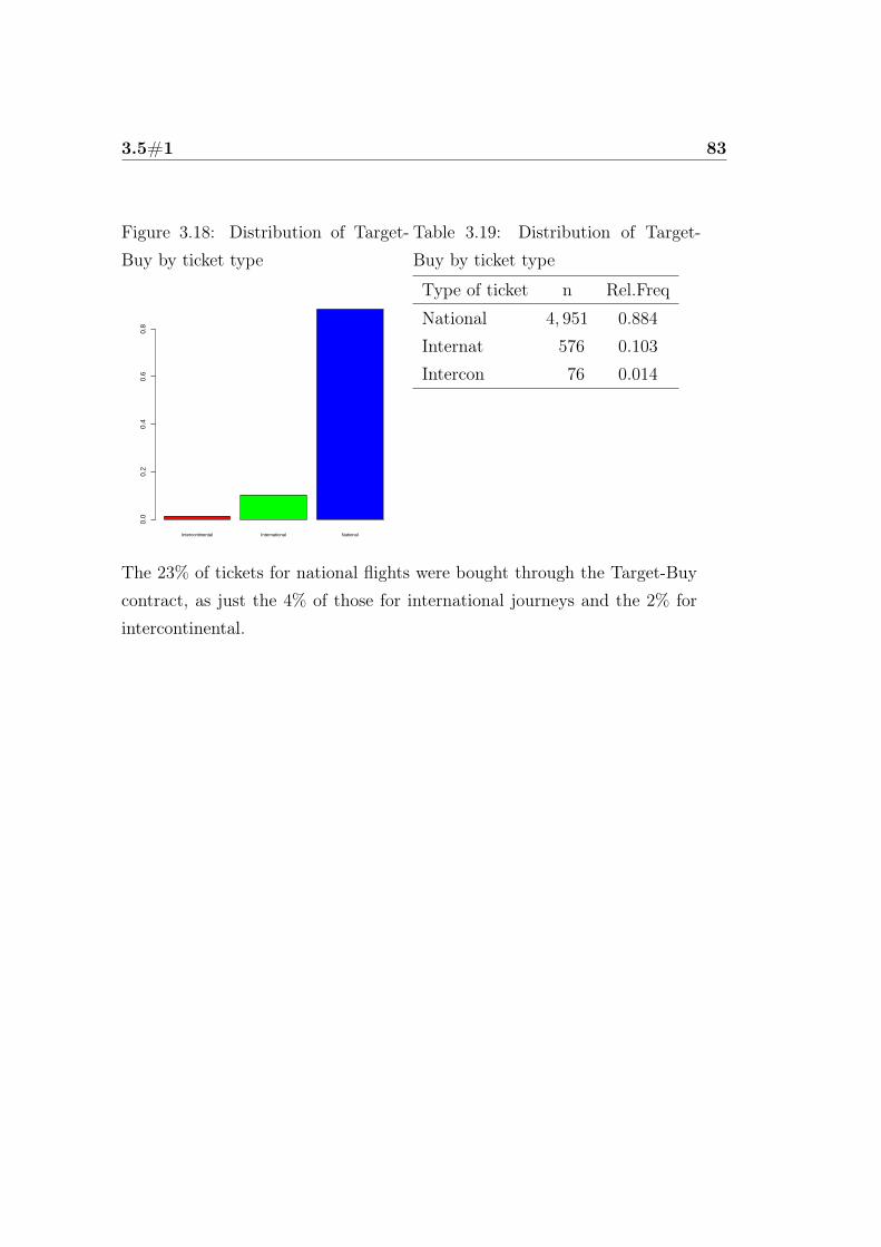
3.5#1 83
Figure 3.18: Distribution of Target-Buy by ticket type
Intercontinental International National
0.0
0.2
0.4
0.6
0.8
Table 3.19: Distribution of Target-Buy by ticket type
Type of ticket n Rel.Freq
National 4, 951 0.884
Internat 576 0.103
Intercon 76 0.014
The 23% of tickets for national flights were bought through the Target-Buycontract, as just the 4% of those for international journeys and the 2% forintercontinental.
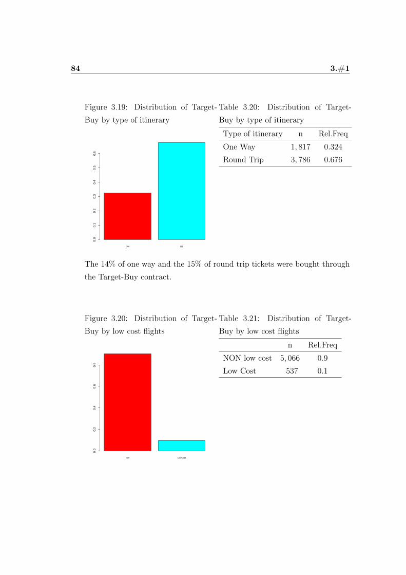
84 3.#1
Figure 3.19: Distribution of Target-Buy by type of itinerary
OW RT
0.0
0.1
0.2
0.3
0.4
0.5
0.6
Table 3.20: Distribution of Target-Buy by type of itinerary
Type of itinerary n Rel.Freq
One Way 1, 817 0.324
Round Trip 3, 786 0.676
The 14% of one way and the 15% of round trip tickets were bought throughthe Target-Buy contract.
Figure 3.20: Distribution of Target-Buy by low cost flights
Non LowCost
0.0
0.2
0.4
0.6
0.8
Table 3.21: Distribution of Target-Buy by low cost flights
n Rel.Freq
NON low cost 5, 066 0.9
Low Cost 537 0.1
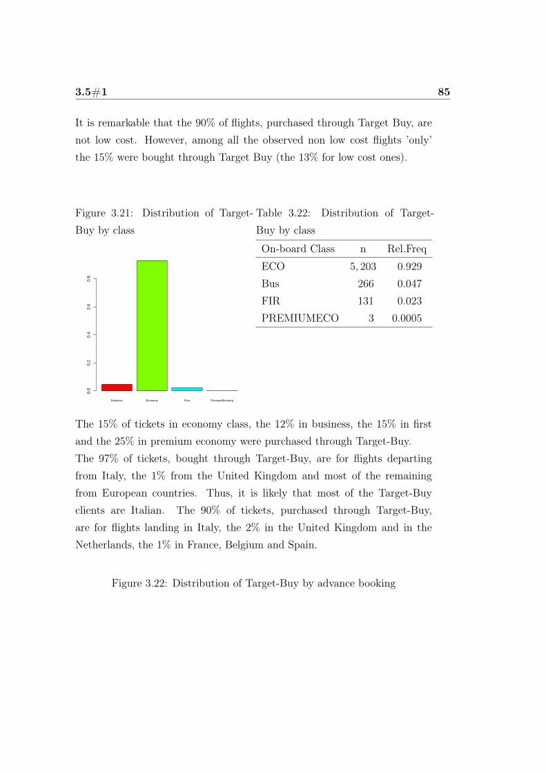
3.5#1 85
It is remarkable that the 90% of flights, purchased through Target Buy, arenot low cost. However, among all the observed non low cost flights ’only’the 15% were bought through Target Buy (the 13% for low cost ones).
Figure 3.21: Distribution of Target-Buy by class
Business Economy First PremiumEconomy
0.0
0.2
0.4
0.6
0.8
Table 3.22: Distribution of Target-Buy by class
On-board Class n Rel.Freq
ECO 5, 203 0.929
Bus 266 0.047
FIR 131 0.023
PREMIUMECO 3 0.0005
The 15% of tickets in economy class, the 12% in business, the 15% in firstand the 25% in premium economy were purchased through Target-Buy.The 97% of tickets, bought through Target-Buy, are for flights departingfrom Italy, the 1% from the United Kingdom and most of the remainingfrom European countries. Thus, it is likely that most of the Target-Buyclients are Italian. The 90% of tickets, purchased through Target-Buy,are for flights landing in Italy, the 2% in the United Kingdom and in theNetherlands, the 1% in France, Belgium and Spain.
Figure 3.22: Distribution of Target-Buy by advance booking
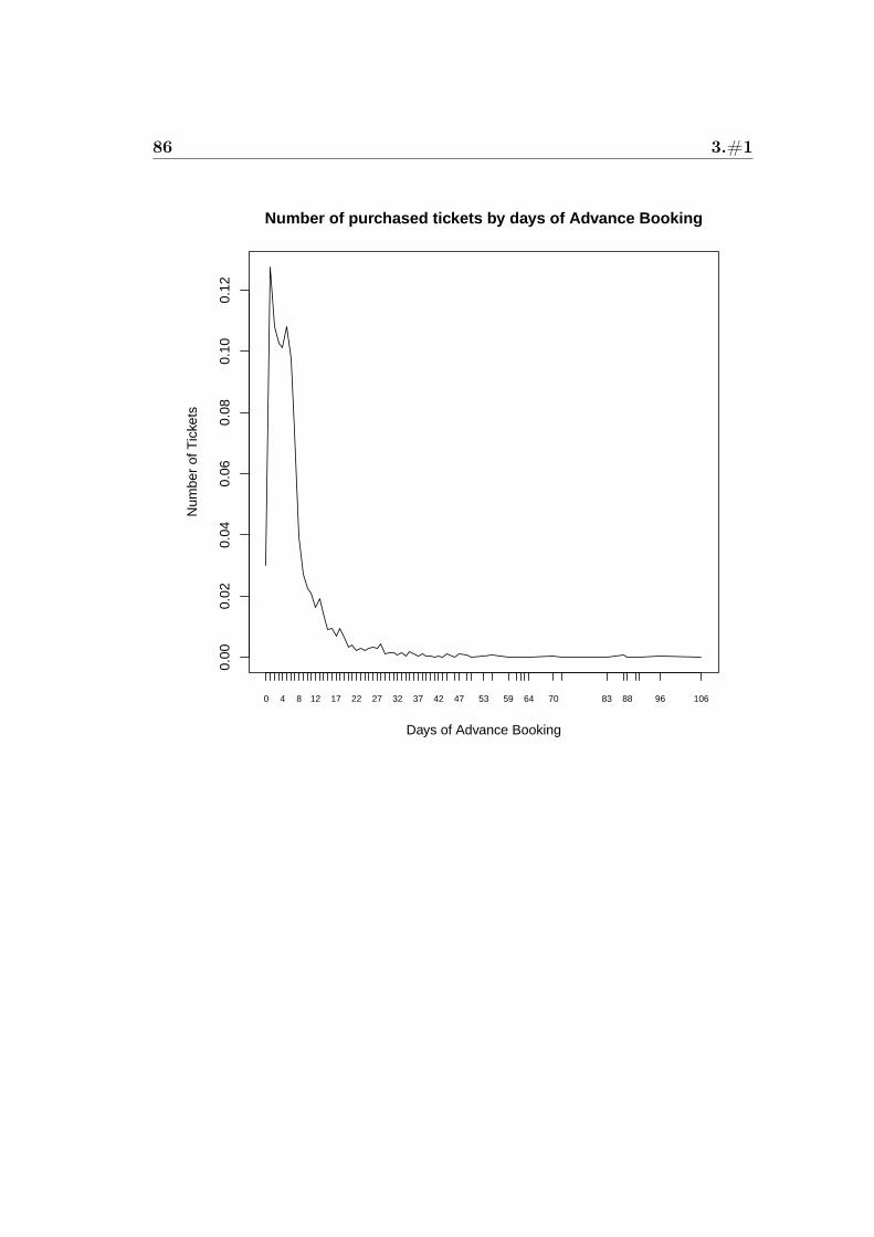
86 3.#1
0.00
0.02
0.04
0.06
0.08
0.10
0.12
Number of purchased tickets by days of Advance Booking
Days of Advance Booking
Num
ber
of T
icke
ts
0 4 8 12 17 22 27 32 37 42 47 53 59 64 70 83 88 96 106
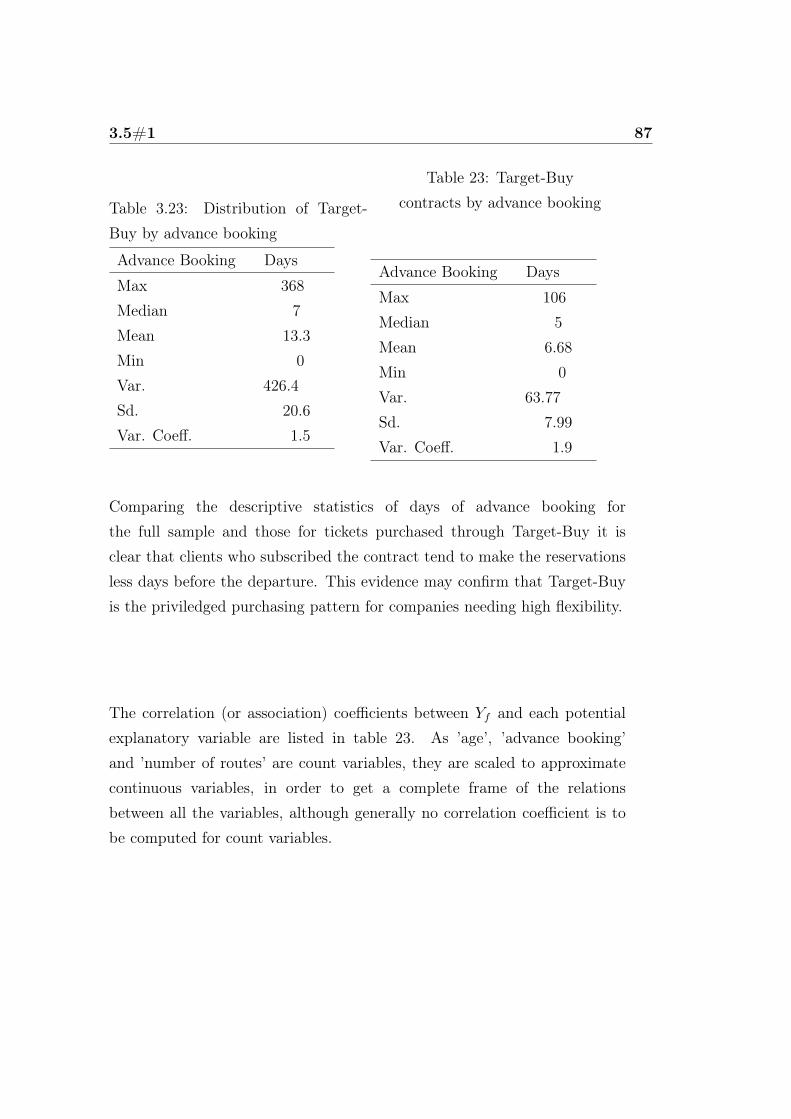
3.5#1 87
Table 3.23: Distribution of Target-Buy by advance booking
Advance Booking Days
Max 368
Median 7
Mean 13.3
Min 0
Var. 426.4
Sd. 20.6
Var. Coeff. 1.5
Table 23: Target-Buycontracts by advance booking
Advance Booking Days
Max 106
Median 5
Mean 6.68
Min 0
Var. 63.77
Sd. 7.99
Var. Coeff. 1.9
Comparing the descriptive statistics of days of advance booking forthe full sample and those for tickets purchased through Target-Buy it isclear that clients who subscribed the contract tend to make the reservationsless days before the departure. This evidence may confirm that Target-Buyis the priviledged purchasing pattern for companies needing high flexibility.
The correlation (or association) coefficients between Yf and each potentialexplanatory variable are listed in table 23. As ’age’, ’advance booking’and ’number of routes’ are count variables, they are scaled to approximatecontinuous variables, in order to get a complete frame of the relationsbetween all the variables, although generally no correlation coefficient is tobe computed for count variables.
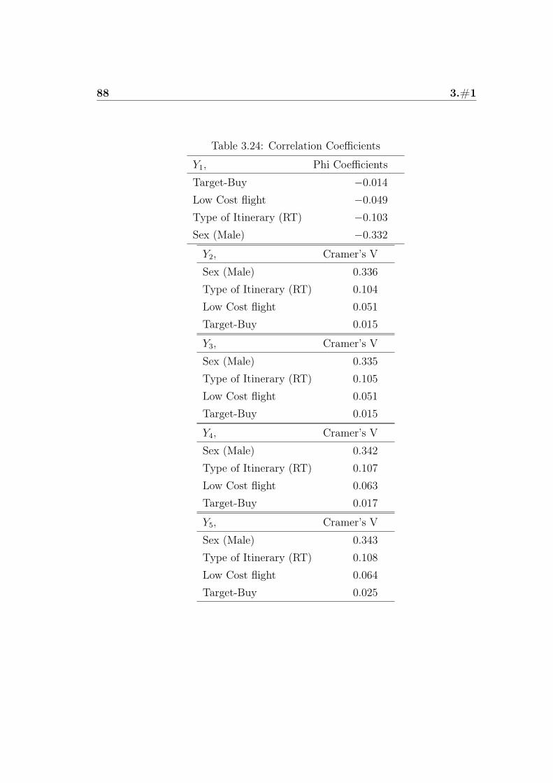
88 3.#1
Table 3.24: Correlation Coefficients
Y1, Phi Coefficients
Target-Buy −0.014
Low Cost flight −0.049
Type of Itinerary (RT) −0.103
Sex (Male) −0.332
Y2, Cramer’s V
Sex (Male) 0.336
Type of Itinerary (RT) 0.104
Low Cost flight 0.051
Target-Buy 0.015
Y3, Cramer’s V
Sex (Male) 0.335Type of Itinerary (RT) 0.105Low Cost flight 0.051Target-Buy 0.015
Y4, Cramer’s V
Sex (Male) 0.342
Type of Itinerary (RT) 0.107
Low Cost flight 0.063
Target-Buy 0.017
Y5, Cramer’s V
Sex (Male) 0.343Type of Itinerary (RT) 0.108Low Cost flight 0.064Target-Buy 0.025
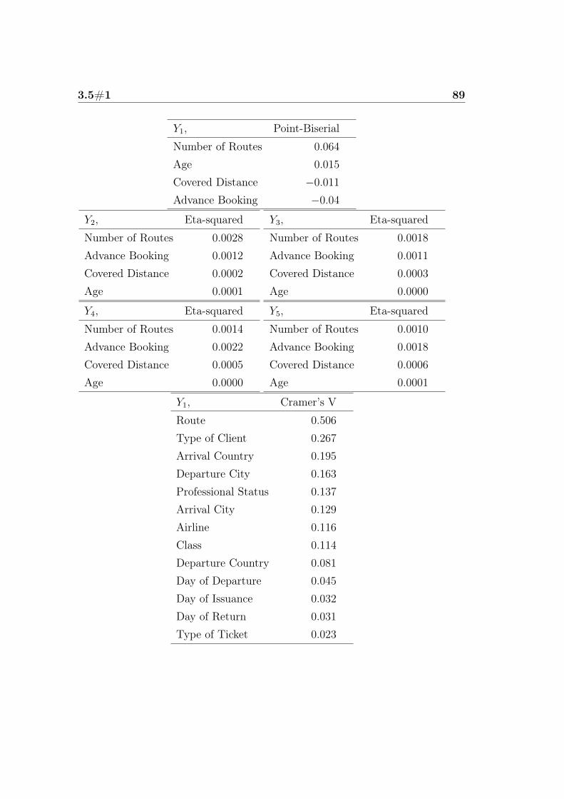
3.5#1 89
Y1, Point-Biserial
Number of Routes 0.064
Age 0.015
Covered Distance −0.011
Advance Booking −0.04
Y2, Eta-squared
Number of Routes 0.0028
Advance Booking 0.0012
Covered Distance 0.0002
Age 0.0001
Y3, Eta-squared
Number of Routes 0.0018
Advance Booking 0.0011
Covered Distance 0.0003
Age 0.0000
Y4, Eta-squared
Number of Routes 0.0014
Advance Booking 0.0022
Covered Distance 0.0005
Age 0.0000
Y5, Eta-squared
Number of Routes 0.0010
Advance Booking 0.0018
Covered Distance 0.0006
Age 0.0001
Y1, Cramer’s V
Route 0.506
Type of Client 0.267
Arrival Country 0.195
Departure City 0.163
Professional Status 0.137
Arrival City 0.129
Airline 0.116
Class 0.114
Departure Country 0.081
Day of Departure 0.045
Day of Issuance 0.032
Day of Return 0.031
Type of Ticket 0.023
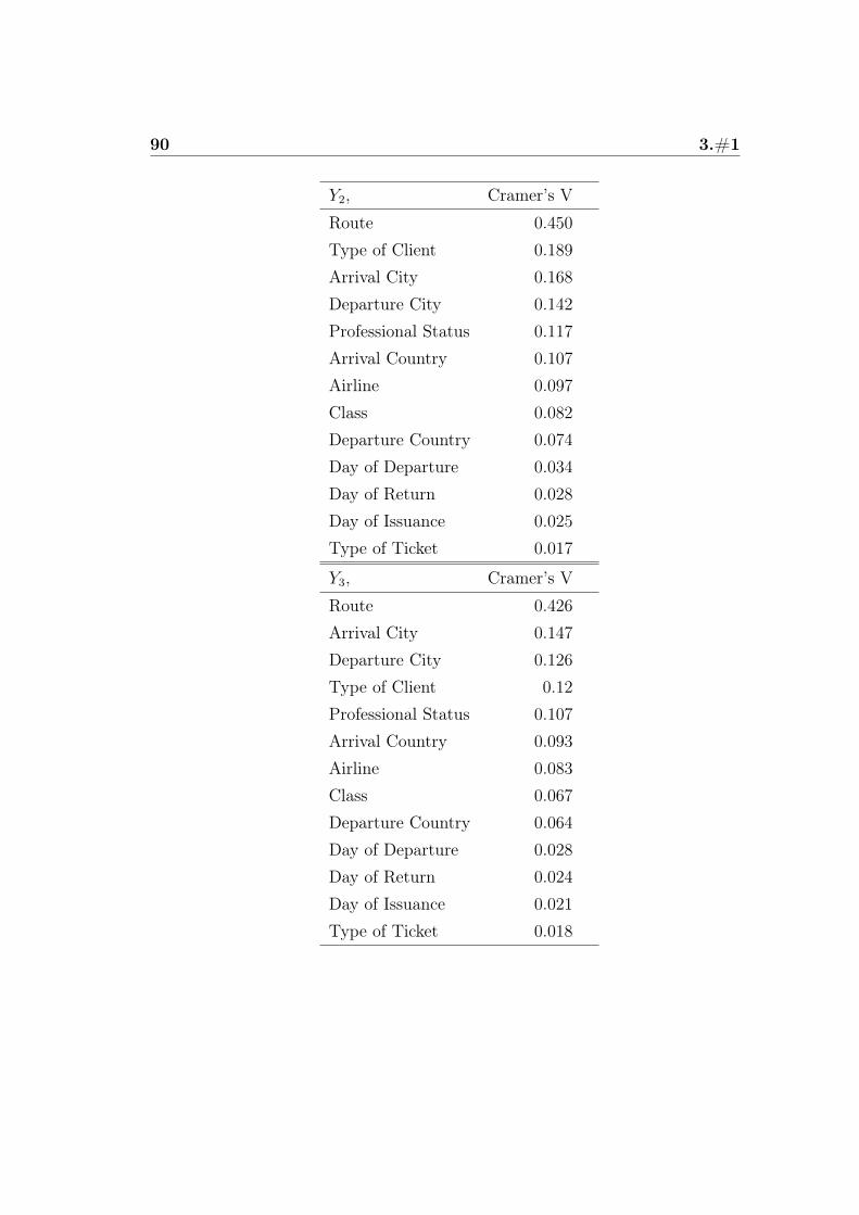
90 3.#1
Y2, Cramer’s V
Route 0.450
Type of Client 0.189
Arrival City 0.168
Departure City 0.142
Professional Status 0.117
Arrival Country 0.107
Airline 0.097
Class 0.082
Departure Country 0.074
Day of Departure 0.034
Day of Return 0.028
Day of Issuance 0.025
Type of Ticket 0.017
Y3, Cramer’s V
Route 0.426
Arrival City 0.147
Departure City 0.126
Type of Client 0.12
Professional Status 0.107
Arrival Country 0.093
Airline 0.083
Class 0.067
Departure Country 0.064
Day of Departure 0.028
Day of Return 0.024
Day of Issuance 0.021
Type of Ticket 0.018
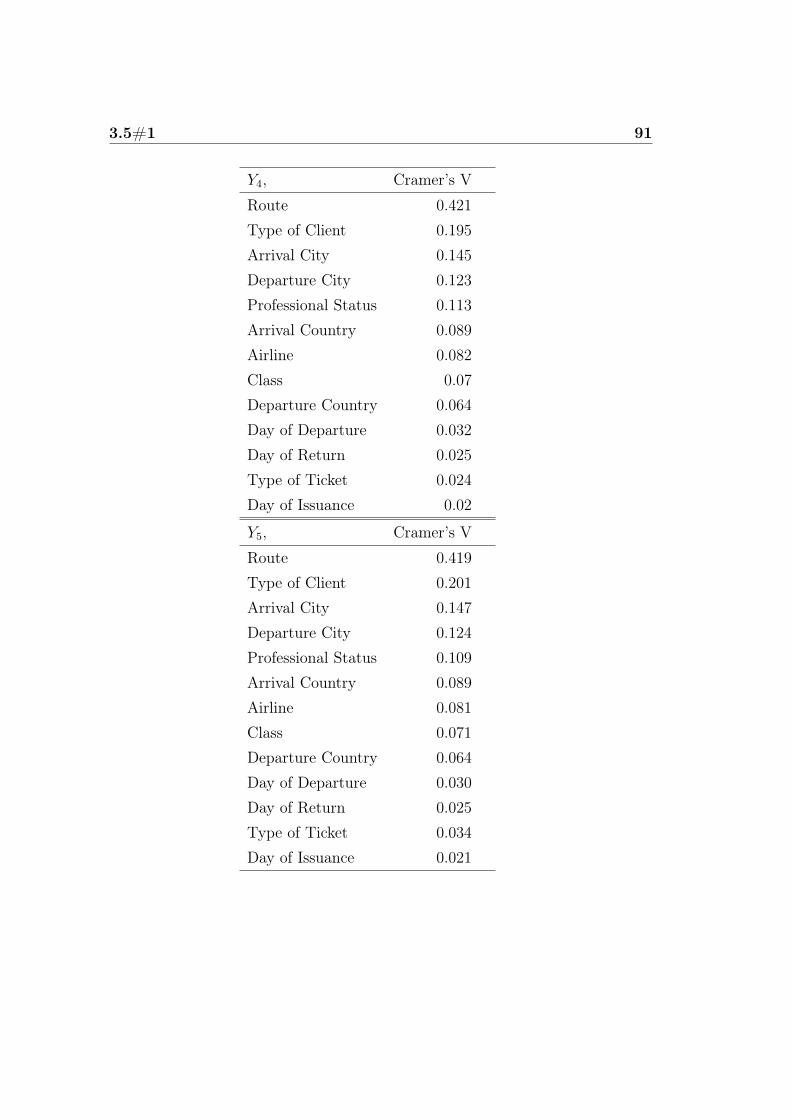
3.5#1 91
Y4, Cramer’s V
Route 0.421
Type of Client 0.195
Arrival City 0.145
Departure City 0.123
Professional Status 0.113
Arrival Country 0.089
Airline 0.082
Class 0.07
Departure Country 0.064
Day of Departure 0.032
Day of Return 0.025
Type of Ticket 0.024
Day of Issuance 0.02
Y5, Cramer’s V
Route 0.419
Type of Client 0.201
Arrival City 0.147
Departure City 0.124
Professional Status 0.109
Arrival Country 0.089
Airline 0.081
Class 0.071
Departure Country 0.064
Day of Departure 0.030
Day of Return 0.025
Type of Ticket 0.034
Day of Issuance 0.021
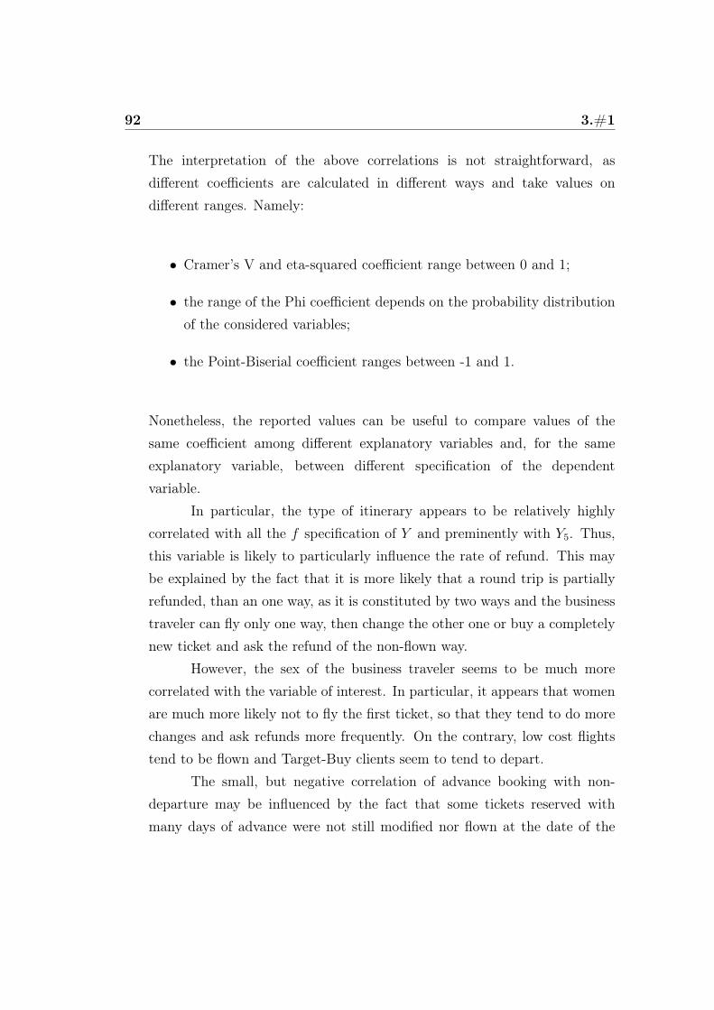
92 3.#1
The interpretation of the above correlations is not straightforward, asdifferent coefficients are calculated in different ways and take values ondifferent ranges. Namely:
• Cramer’s V and eta-squared coefficient range between 0 and 1;
• the range of the Phi coefficient depends on the probability distributionof the considered variables;
• the Point-Biserial coefficient ranges between -1 and 1.
Nonetheless, the reported values can be useful to compare values of thesame coefficient among different explanatory variables and, for the sameexplanatory variable, between different specification of the dependentvariable.
In particular, the type of itinerary appears to be relatively highlycorrelated with all the f specification of Y and preminently with Y5. Thus,this variable is likely to particularly influence the rate of refund. This maybe explained by the fact that it is more likely that a round trip is partiallyrefunded, than an one way, as it is constituted by two ways and the businesstraveler can fly only one way, then change the other one or buy a completelynew ticket and ask the refund of the non-flown way.
However, the sex of the business traveler seems to be much morecorrelated with the variable of interest. In particular, it appears that womenare much more likely not to fly the first ticket, so that they tend to do morechanges and ask refunds more frequently. On the contrary, low cost flightstend to be flown and Target-Buy clients seem to tend to depart.
The small, but negative correlation of advance booking with non-departure may be influenced by the fact that some tickets reserved withmany days of advance were not still modified nor flown at the date of the

3.5#1 93
data collection (right censoring). A similar relation seems to hold betweenthe tendency not to fly the first ticket and the covered distance. Thisevidence may be explained hypothesizing that the longer the journey theless easily it can be re-organized, for another date, for example. Indeed,this consideration may be in contrast with the values of the correlationcoefficients for the number of routes. But it is not to be taken for grantedthat a higher number of routes implies a wider covered distance.
In general, it seems that the variable "route" is the most related withthe risk of non-fly. The type of client company can also be an importantpredictor for such a risk. The places of arrival appear to be more relatedwith the behavior of the business traveler than the places of departure.Thus, maybe the characteristics of the journey influence the risk of ticketchange/refund more than the client company (the nationality of which israther related with the departure place).
However, a measure of association comparable between differentspecifications of the dependent variable and between all of the candidateregressors is more useful, especially to lead the aggregation of categoricalvariables’ levels and the definitive specification of the dependent variable.Thus, the P-values of chi-squared tests for independence are reported below.
Table 3.25: P-values of chi-squared tests
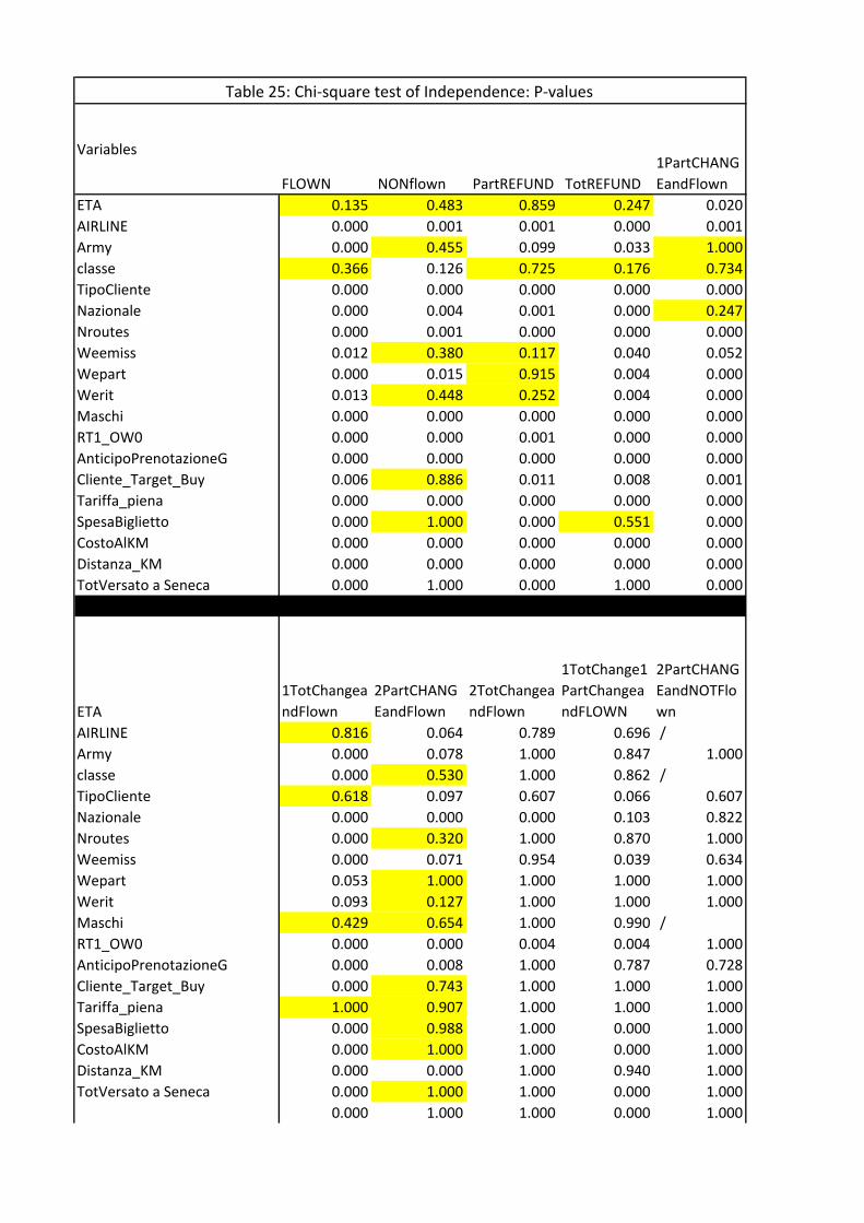
Variables
FLOWN NONflown PartREFUND TotREFUND
1PartCHANG
EandFlown
ETA 0.135 0.483 0.859 0.247 0.020
AIRLINE 0.000 0.001 0.001 0.000 0.001
Army 0.000 0.455 0.099 0.033 1.000
classe 0.366 0.126 0.725 0.176 0.734
TipoCliente 0.000 0.000 0.000 0.000 0.000
Nazionale 0.000 0.004 0.001 0.000 0.247
Nroutes 0.000 0.001 0.000 0.000 0.000
Weemiss 0.012 0.380 0.117 0.040 0.052
Wepart 0.000 0.015 0.915 0.004 0.000
Werit 0.013 0.448 0.252 0.004 0.000
Maschi 0.000 0.000 0.000 0.000 0.000
RT1_OW0 0.000 0.000 0.001 0.000 0.000
AnticipoPrenotazioneG 0.000 0.000 0.000 0.000 0.000
Cliente_Target_Buy 0.006 0.886 0.011 0.008 0.001
Tariffa_piena 0.000 0.000 0.000 0.000 0.000
SpesaBiglietto 0.000 1.000 0.000 0.551 0.000
CostoAlKM 0.000 0.000 0.000 0.000 0.000
Distanza_KM 0.000 0.000 0.000 0.000 0.000
TotVersato a Seneca 0.000 1.000 0.000 1.000 0.000
ETA
1TotChangea
ndFlown
2PartCHANG
EandFlown
2TotChangea
ndFlown
1TotChange1
PartChangea
ndFLOWN
2PartCHANG
EandNOTFlo
wn
AIRLINE 0.816 0.064 0.789 0.696 /
Army 0.000 0.078 1.000 0.847 1.000
classe 0.000 0.530 1.000 0.862 /
TipoCliente 0.618 0.097 0.607 0.066 0.607
Nazionale 0.000 0.000 0.000 0.103 0.822
Nroutes 0.000 0.320 1.000 0.870 1.000
Weemiss 0.000 0.071 0.954 0.039 0.634
Wepart 0.053 1.000 1.000 1.000 1.000
Werit 0.093 0.127 1.000 1.000 1.000
Maschi 0.429 0.654 1.000 0.990 /
RT1_OW0 0.000 0.000 0.004 0.004 1.000
AnticipoPrenotazioneG 0.000 0.008 1.000 0.787 0.728
Cliente_Target_Buy 0.000 0.743 1.000 1.000 1.000
Tariffa_piena 1.000 0.907 1.000 1.000 1.000
SpesaBiglietto 0.000 0.988 1.000 0.000 1.000
CostoAlKM 0.000 1.000 1.000 0.000 1.000
Distanza_KM 0.000 0.000 1.000 0.940 1.000
TotVersato a Seneca 0.000 1.000 1.000 0.000 1.000
0.000 1.000 1.000 0.000 1.000
Table 25: Chi-square test of Independence: P-values
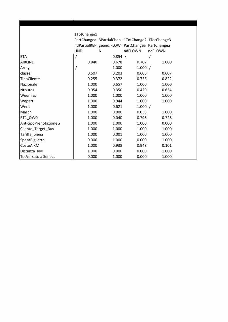
1TotChange1
PartChangea
ndPartialREF
UND
3PartialChan
geand.FLOW
N
1TotChange2
PartChangea
ndFLOWN
1TotChange3
PartChangea
ndFLOWN
ETA / 0.854 / /
AIRLINE 0.840 0.678 0.707 1.000
Army / 1.000 1.000 /
classe 0.607 0.203 0.606 0.607
TipoCliente 0.255 0.372 0.756 0.822
Nazionale 1.000 0.657 1.000 1.000
Nroutes 0.954 0.350 0.420 0.634
Weemiss 1.000 1.000 1.000 1.000
Wepart 1.000 0.944 1.000 1.000
Werit 1.000 0.621 1.000 /
Maschi 1.000 0.000 0.053 1.000
RT1_OW0 1.000 0.040 0.798 0.728
AnticipoPrenotazioneG 1.000 1.000 1.000 0.000
Cliente_Target_Buy 1.000 1.000 1.000 1.000
Tariffa_piena 1.000 0.001 1.000 1.000
SpesaBiglietto 0.000 1.000 0.000 1.000
CostoAlKM 1.000 0.938 0.948 0.101
Distanza_KM 1.000 0.000 0.000 1.000
TotVersato a Seneca 0.000 1.000 0.000 1.000

96 3.#1
Then, variables are aggregated and selected (within sets of overlap-ping/equivalent ones, see above) combining logical considerations, sign andsignificance of the chi-squared association and results of a more naive anal-ysis, based on the difference between the conditional distribution of Yf , toeach single level of each single variable, and the marginal distribution of Yf ,displayed below (if the difference is zero, then the two variables are absolutelyindependent in distribution).
Table 3.26: Differences from the marginal masses
MARGINAL 1 0.852 0.008 0.020 0.014 0.077 0.027
n FLOWN NONflown PartREFUNDTotREFUNDPartCh TotCh
BANK 421 -0.842 0.037 0.208 0.065 0.393 0.109
CORPORATE 26079 0.031 -0.001 -0.003 0.004 -0.032 0.001
PA 9811 0.059 -0.003 0.003 -0.010 -0.034 -0.017
n FLOWN NONflown PartREFUNDTotREFUNDPartCh TotCh
n FLOWN NONflown PartREFUNDTotREFUNDPartCh TotCh
OPERAIO 1 -0.852 -0.008 -0.020 -0.014 0.923 -0.027
PROF 32 -0.852 0.023 0.042 -0.014 0.704 0.036
HOST 13 -0.775 0.146 0.056 -0.014 0.615 -0.027
UFFICIALIinferiori 19 -0.799 -0.008 0.137 -0.014 0.607 -0.027
MAGISTRATO 3 -0.852 -0.008 0.313 -0.014 0.590 -0.027
IMPIEGATO 700 -0.806 0.044 0.101 0.028 0.517 0.100
GENERALE 19 -0.746 0.098 0.085 -0.014 0.502 0.026
GRADUATI 30 -0.652 0.026 0.146 0.020 0.490 -0.027
PROFESSIONISTA 9 -0.852 -0.008 0.091 -0.014 0.479 0.306
DIRETTOREadPres 50 -0.812 0.052 0.120 0.126 0.443 0.033
UFFICIALIsuperiori 10 -0.552 -0.008 0.180 -0.014 0.423 -0.027
DIRIGENTE 1073 -0.810 0.030 0.110 0.074 0.422 0.160
QUADRO 556 -0.821 0.048 0.118 0.087 0.420 0.124
SOTTOufficiali 34 -0.705 -0.008 0.244 0.016 0.364 0.003
TITOLARE 14 -0.852 -0.008 0.122 0.058 0.352 0.330
n FLOWN NONflown PartREFUNDTotREFUNDPartCh TotCh
Nazionale 21273 -0.007 0.001 -0.002 0.003 0.002 0.004
Internazionale 14013 0.010 -0.001 0.002 -0.004 -0.001 -0.006
Intercontinentale 3603 0.003 -0.002 0.007 -0.003 -0.006 0.000
n FLOWN NONflown PartREFUNDTotREFUNDPartCh TotCh
7 3 -0.185 -0.008 -0.020 -0.014 0.256 -0.027
5 114 -0.062 -0.008 0.023 -0.014 0.046 0.008
1 10917 -0.061 0.003 0.002 0.007 0.039 0.009
6 114 -0.071 0.001 0.050 0.013 -0.007 0.017
2 23165 0.025 -0.001 -0.002 -0.004 -0.014 -0.005
3 729 0.030 -0.004 0.007 -0.001 -0.019 -0.013
4 3846 0.020 -0.003 0.000 0.003 -0.024 0.004
8 1 -0.852 -0.008 -0.020 0.986 -0.077 -0.027
n FLOWN NONflown PartREFUNDTotREFUNDPartCh TotCh
Mar 7790 -0.020 0.001 0.002 0.004 0.006 0.007
Mer 7915 0.002 0.000 -0.002 0.002 0.000 -0.002
Lun 7101 -0.002 -0.001 0.000 0.000 -0.001 0.003
Ven 7879 0.008 -0.001 0.001 -0.002 -0.001 -0.005
Giov 7488 0.009 0.001 -0.001 -0.003 -0.002 -0.003
Dom 216 0.037 -0.008 -0.002 -0.014 -0.003 -0.013
Sab 500 0.032 -0.002 0.014 -0.008 -0.027 -0.013
n FLOWN NONflown PartREFUNDTotREFUNDPartCh TotCh
Ven 4426 -0.005 0.001 0.000 -0.004 0.014 -0.008
Giov 5597 -0.008 -0.001 -0.001 0.002 0.005 0.002
Mer 7486 -0.021 0.003 0.001 0.005 0.001 0.012
Lun 8590 0.017 -0.001 -0.003 -0.004 -0.001 -0.008
Mar 7965 -0.006 0.001 0.002 0.002 -0.003 0.003
Table 26: differences between conditional and marginal distributions

Sab 1505 0.021 -0.004 -0.001 -0.004 -0.009 -0.002
Dom 3320 0.030 -0.003 0.001 -0.005 -0.018 -0.005
n FLOWN NONflown PartREFUNDTotREFUNDPartCh TotCh
Dom 1551 -0.004 -0.002 -0.002 -0.005 0.017 -0.004
Ven 5908 0.017 -0.001 -0.002 0.000 -0.011 -0.002
Lun 2876 0.040 0.000 -0.007 -0.005 -0.018 -0.009
Mar 3723 0.030 -0.002 -0.003 -0.002 -0.019 -0.004
Sab 1417 0.028 -0.003 0.004 -0.011 -0.021 0.004
Giov 5511 0.027 -0.001 -0.002 -0.002 -0.021 -0.001
Mer 4984 0.031 0.000 0.000 -0.002 -0.027 -0.002
n FLOWN NONflown PartREFUNDTotREFUNDPartCh TotCh
Maschi 28072 -0.029 0.001 0.004 0.002 0.018 0.004
n FLOWN NONflown PartREFUNDTotREFUNDPartCh TotCh
Cliente_Target_Buy 5603 0.012 0.000 -0.005 0.004 -0.011 0.000
n FLOWN NONflown PartREFUNDTotREFUNDPartCh TotCh
RT1_OW0 25834 0.026 -0.001 -0.002 -0.003 -0.017 -0.003
n FLOWN NONflown PartREFUNDTotREFUNDPartCh TotCh
2 2173 0.016 -0.002 0.000 -0.007 0.000 -0.006
1 1058 0.033 -0.006 -0.002 -0.006 -0.010 -0.009
4 1512 0.032 -0.003 -0.003 -0.001 -0.017 -0.008
3 3195 0.040 -0.001 -0.004 -0.007 -0.018 -0.009
n FLOWN NONflown PartREFUNDTotREFUNDPartCh TotCh
Eco 9718 -0.002 0.001 0.001 -0.001 0.001 0.000
Bus 19450 -0.001 -0.001 0.000 0.001 0.001 0.001
Fir 9720 0.004 0.001 0.000 -0.001 -0.003 -0.001
n FLOWN NONflown PartREFUNDTotREFUNDPartCh TotCh
LowCost 1044 -0.006 0.003 0.000 -0.004 0.020 -0.015
MERIDIANA_FLY 905 0.021 -0.003 -0.006 -0.009 0.019 -0.020
BRITISH_AIRWAYS 601 0.000 -0.004 0.005 -0.009 0.008 0.000
Other 6559 0.005 -0.002 0.004 -0.005 0.003 -0.005
ALITALIA_CAI_SPA 21838 -0.012 0.001 0.000 0.004 0.001 0.007
AIR_FRANCE 939 -0.037 0.003 0.011 0.013 0.000 0.008
LUFTHANSA 2615 0.002 0.000 0.001 0.002 -0.008 0.002
BRUSSELS_AIRLINES 1260 0.025 0.000 0.000 -0.009 -0.009 -0.012
RYANAIR 1486 0.069 -0.006 -0.012 -0.014 -0.010 -0.025
EASYJET 1642 0.073 -0.005 -0.008 -0.013 -0.020 -0.025
n FLOWN NONflown PartREFUNDTotREFUNDPartCh TotCh
Cuneo 32 -0.508 -0.008 0.073 0.205 0.204 0.036
Miami 17 -0.323 -0.008 0.215 -0.014 0.158 -0.027
Stuttgart 13 -0.083 -0.008 -0.020 -0.014 0.154 -0.027
Shanghai 18 -0.130 -0.008 0.035 -0.014 0.145 -0.027
Munich 45 -0.118 -0.008 0.002 0.008 0.123 -0.004
Sao_Paulo 28 -0.102 -0.008 0.015 -0.014 0.102 0.009
Bremen 17 -0.146 -0.008 -0.020 -0.014 0.100 0.032
Moscow 40 -0.077 -0.008 0.005 0.011 0.098 -0.027
Malta 23 -0.200 -0.008 0.154 -0.014 0.097 -0.027
Helsinki 29 -0.093 -0.008 0.014 0.021 0.096 -0.027
Dublin 30 -0.052 -0.008 0.013 -0.014 0.090 -0.027
Heraklion 121 -0.108 0.001 -0.004 0.019 0.080 0.015
WINNIPEG 13 -0.006 -0.008 -0.020 -0.014 0.077 -0.027
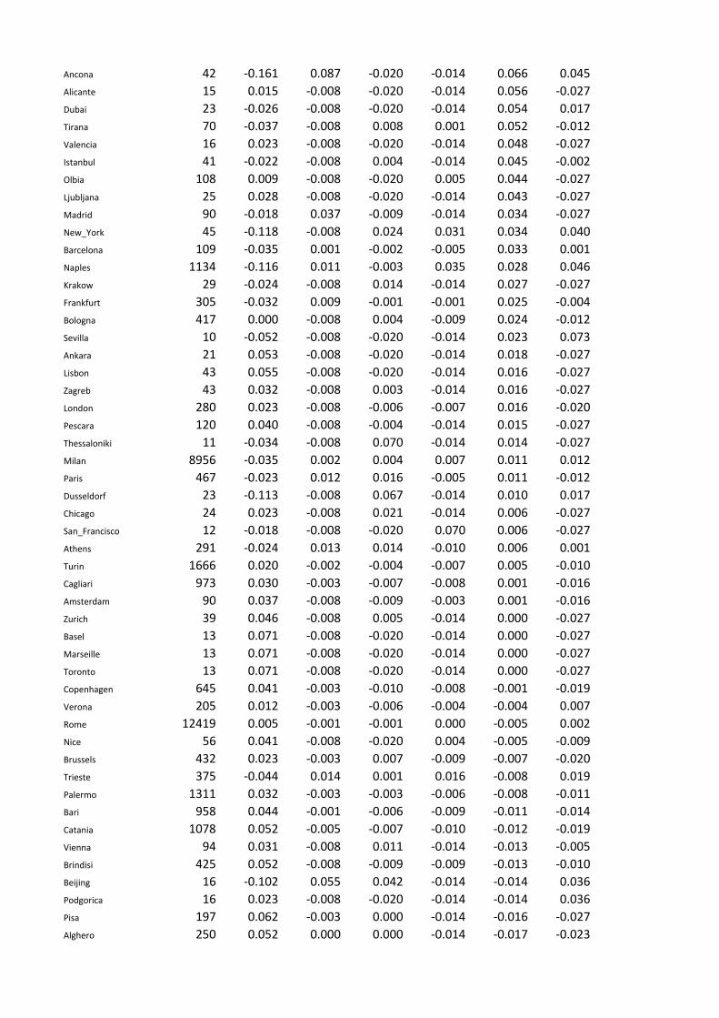
Ancona 42 -0.161 0.087 -0.020 -0.014 0.066 0.045
Alicante 15 0.015 -0.008 -0.020 -0.014 0.056 -0.027
Dubai 23 -0.026 -0.008 -0.020 -0.014 0.054 0.017
Tirana 70 -0.037 -0.008 0.008 0.001 0.052 -0.012
Valencia 16 0.023 -0.008 -0.020 -0.014 0.048 -0.027
Istanbul 41 -0.022 -0.008 0.004 -0.014 0.045 -0.002
Olbia 108 0.009 -0.008 -0.020 0.005 0.044 -0.027
Ljubljana 25 0.028 -0.008 -0.020 -0.014 0.043 -0.027
Madrid 90 -0.018 0.037 -0.009 -0.014 0.034 -0.027
New_York 45 -0.118 -0.008 0.024 0.031 0.034 0.040
Barcelona 109 -0.035 0.001 -0.002 -0.005 0.033 0.001
Naples 1134 -0.116 0.011 -0.003 0.035 0.028 0.046
Krakow 29 -0.024 -0.008 0.014 -0.014 0.027 -0.027
Frankfurt 305 -0.032 0.009 -0.001 -0.001 0.025 -0.004
Bologna 417 0.000 -0.008 0.004 -0.009 0.024 -0.012
Sevilla 10 -0.052 -0.008 -0.020 -0.014 0.023 0.073
Ankara 21 0.053 -0.008 -0.020 -0.014 0.018 -0.027
Lisbon 43 0.055 -0.008 -0.020 -0.014 0.016 -0.027
Zagreb 43 0.032 -0.008 0.003 -0.014 0.016 -0.027
London 280 0.023 -0.008 -0.006 -0.007 0.016 -0.020
Pescara 120 0.040 -0.008 -0.004 -0.014 0.015 -0.027
Thessaloniki 11 -0.034 -0.008 0.070 -0.014 0.014 -0.027
Milan 8956 -0.035 0.002 0.004 0.007 0.011 0.012
Paris 467 -0.023 0.012 0.016 -0.005 0.011 -0.012
Dusseldorf 23 -0.113 -0.008 0.067 -0.014 0.010 0.017
Chicago 24 0.023 -0.008 0.021 -0.014 0.006 -0.027
San_Francisco 12 -0.018 -0.008 -0.020 0.070 0.006 -0.027
Athens 291 -0.024 0.013 0.014 -0.010 0.006 0.001
Turin 1666 0.020 -0.002 -0.004 -0.007 0.005 -0.010
Cagliari 973 0.030 -0.003 -0.007 -0.008 0.001 -0.016
Amsterdam 90 0.037 -0.008 -0.009 -0.003 0.001 -0.016
Zurich 39 0.046 -0.008 0.005 -0.014 0.000 -0.027
Basel 13 0.071 -0.008 -0.020 -0.014 0.000 -0.027
Marseille 13 0.071 -0.008 -0.020 -0.014 0.000 -0.027
Toronto 13 0.071 -0.008 -0.020 -0.014 0.000 -0.027
Copenhagen 645 0.041 -0.003 -0.010 -0.008 -0.001 -0.019
Verona 205 0.012 -0.003 -0.006 -0.004 -0.004 0.007
Rome 12419 0.005 -0.001 -0.001 0.000 -0.005 0.002
Nice 56 0.041 -0.008 -0.020 0.004 -0.005 -0.009
Brussels 432 0.023 -0.003 0.007 -0.009 -0.007 -0.020
Trieste 375 -0.044 0.014 0.001 0.016 -0.008 0.019
Palermo 1311 0.032 -0.003 -0.003 -0.006 -0.008 -0.011
Bari 958 0.044 -0.001 -0.006 -0.009 -0.011 -0.014
Catania 1078 0.052 -0.005 -0.007 -0.010 -0.012 -0.019
Vienna 94 0.031 -0.008 0.011 -0.014 -0.013 -0.005
Brindisi 425 0.052 -0.008 -0.009 -0.009 -0.013 -0.010
Beijing 16 -0.102 0.055 0.042 -0.014 -0.014 0.036
Podgorica 16 0.023 -0.008 -0.020 -0.014 -0.014 0.036
Pisa 197 0.062 -0.003 0.000 -0.014 -0.016 -0.027
Alghero 250 0.052 0.000 0.000 -0.014 -0.017 -0.023
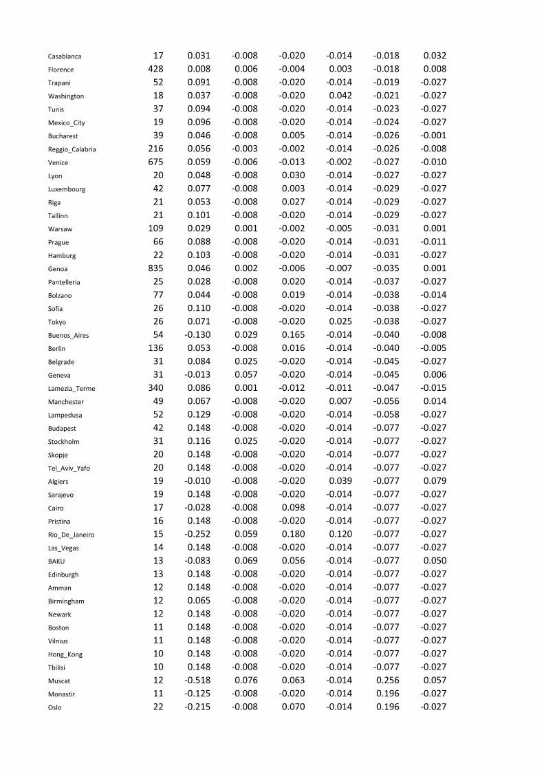
Casablanca 17 0.031 -0.008 -0.020 -0.014 -0.018 0.032
Florence 428 0.008 0.006 -0.004 0.003 -0.018 0.008
Trapani 52 0.091 -0.008 -0.020 -0.014 -0.019 -0.027
Washington 18 0.037 -0.008 -0.020 0.042 -0.021 -0.027
Tunis 37 0.094 -0.008 -0.020 -0.014 -0.023 -0.027
Mexico_City 19 0.096 -0.008 -0.020 -0.014 -0.024 -0.027
Bucharest 39 0.046 -0.008 0.005 -0.014 -0.026 -0.001
Reggio_Calabria 216 0.056 -0.003 -0.002 -0.014 -0.026 -0.008
Venice 675 0.059 -0.006 -0.013 -0.002 -0.027 -0.010
Lyon 20 0.048 -0.008 0.030 -0.014 -0.027 -0.027
Luxembourg 42 0.077 -0.008 0.003 -0.014 -0.029 -0.027
Riga 21 0.053 -0.008 0.027 -0.014 -0.029 -0.027
Tallinn 21 0.101 -0.008 -0.020 -0.014 -0.029 -0.027
Warsaw 109 0.029 0.001 -0.002 -0.005 -0.031 0.001
Prague 66 0.088 -0.008 -0.020 -0.014 -0.031 -0.011
Hamburg 22 0.103 -0.008 -0.020 -0.014 -0.031 -0.027
Genoa 835 0.046 0.002 -0.006 -0.007 -0.035 0.001
Pantelleria 25 0.028 -0.008 0.020 -0.014 -0.037 -0.027
Bolzano 77 0.044 -0.008 0.019 -0.014 -0.038 -0.014
Sofia 26 0.110 -0.008 -0.020 -0.014 -0.038 -0.027
Tokyo 26 0.071 -0.008 -0.020 0.025 -0.038 -0.027
Buenos_Aires 54 -0.130 0.029 0.165 -0.014 -0.040 -0.008
Berlin 136 0.053 -0.008 0.016 -0.014 -0.040 -0.005
Belgrade 31 0.084 0.025 -0.020 -0.014 -0.045 -0.027
Geneva 31 -0.013 0.057 -0.020 -0.014 -0.045 0.006
Lamezia_Terme 340 0.086 0.001 -0.012 -0.011 -0.047 -0.015
Manchester 49 0.067 -0.008 -0.020 0.007 -0.056 0.014
Lampedusa 52 0.129 -0.008 -0.020 -0.014 -0.058 -0.027
Budapest 42 0.148 -0.008 -0.020 -0.014 -0.077 -0.027
Stockholm 31 0.116 0.025 -0.020 -0.014 -0.077 -0.027
Skopje 20 0.148 -0.008 -0.020 -0.014 -0.077 -0.027
Tel_Aviv_Yafo 20 0.148 -0.008 -0.020 -0.014 -0.077 -0.027
Algiers 19 -0.010 -0.008 -0.020 0.039 -0.077 0.079
Sarajevo 19 0.148 -0.008 -0.020 -0.014 -0.077 -0.027
Cairo 17 -0.028 -0.008 0.098 -0.014 -0.077 -0.027
Pristina 16 0.148 -0.008 -0.020 -0.014 -0.077 -0.027
Rio_De_Janeiro 15 -0.252 0.059 0.180 0.120 -0.077 -0.027
Las_Vegas 14 0.148 -0.008 -0.020 -0.014 -0.077 -0.027
BAKU 13 -0.083 0.069 0.056 -0.014 -0.077 0.050
Edinburgh 13 0.148 -0.008 -0.020 -0.014 -0.077 -0.027
Amman 12 0.148 -0.008 -0.020 -0.014 -0.077 -0.027
Birmingham 12 0.065 -0.008 -0.020 -0.014 -0.077 -0.027
Newark 12 0.148 -0.008 -0.020 -0.014 -0.077 -0.027
Boston 11 0.148 -0.008 -0.020 -0.014 -0.077 -0.027
Vilnius 11 0.148 -0.008 -0.020 -0.014 -0.077 -0.027
Hong_Kong 10 0.148 -0.008 -0.020 -0.014 -0.077 -0.027
Tbilisi 10 0.148 -0.008 -0.020 -0.014 -0.077 -0.027
Muscat 12 -0.518 0.076 0.063 -0.014 0.256 0.057
Monastir 11 -0.125 -0.008 -0.020 -0.014 0.196 -0.027
Oslo 22 -0.215 -0.008 0.070 -0.014 0.196 -0.027
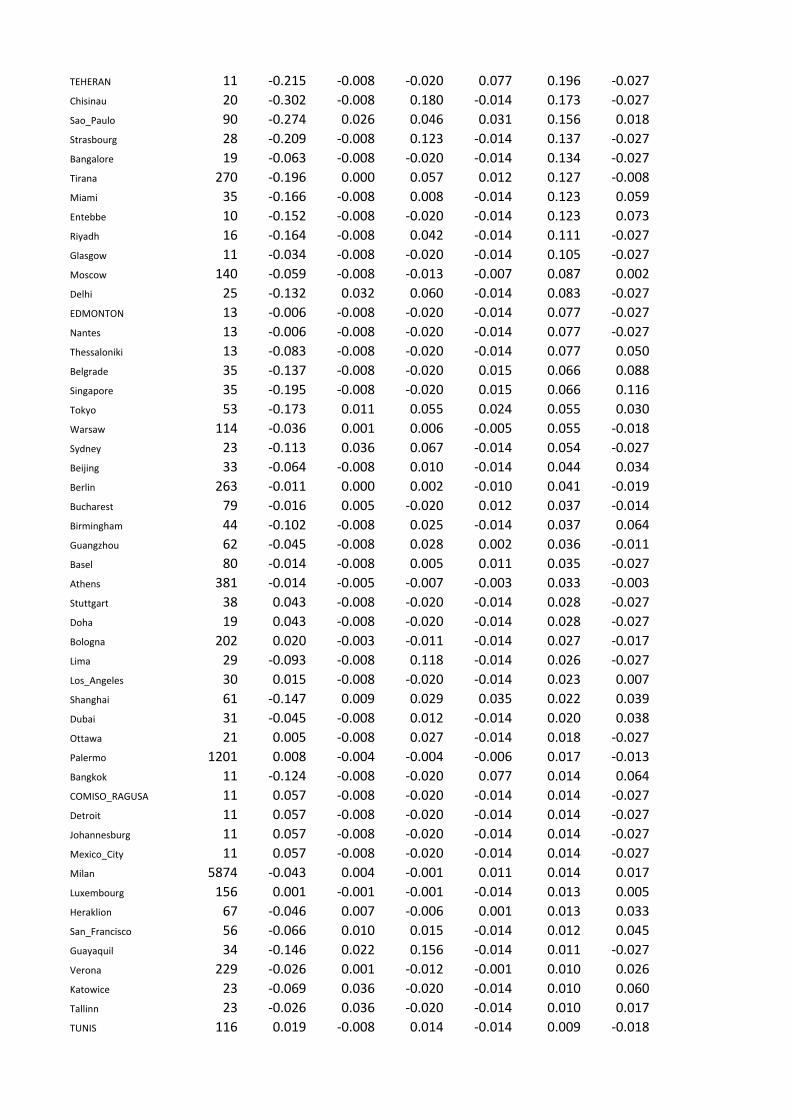
TEHERAN 11 -0.215 -0.008 -0.020 0.077 0.196 -0.027
Chisinau 20 -0.302 -0.008 0.180 -0.014 0.173 -0.027
Sao_Paulo 90 -0.274 0.026 0.046 0.031 0.156 0.018
Strasbourg 28 -0.209 -0.008 0.123 -0.014 0.137 -0.027
Bangalore 19 -0.063 -0.008 -0.020 -0.014 0.134 -0.027
Tirana 270 -0.196 0.000 0.057 0.012 0.127 -0.008
Miami 35 -0.166 -0.008 0.008 -0.014 0.123 0.059
Entebbe 10 -0.152 -0.008 -0.020 -0.014 0.123 0.073
Riyadh 16 -0.164 -0.008 0.042 -0.014 0.111 -0.027
Glasgow 11 -0.034 -0.008 -0.020 -0.014 0.105 -0.027
Moscow 140 -0.059 -0.008 -0.013 -0.007 0.087 0.002
Delhi 25 -0.132 0.032 0.060 -0.014 0.083 -0.027
EDMONTON 13 -0.006 -0.008 -0.020 -0.014 0.077 -0.027
Nantes 13 -0.006 -0.008 -0.020 -0.014 0.077 -0.027
Thessaloniki 13 -0.083 -0.008 -0.020 -0.014 0.077 0.050
Belgrade 35 -0.137 -0.008 -0.020 0.015 0.066 0.088
Singapore 35 -0.195 -0.008 -0.020 0.015 0.066 0.116
Tokyo 53 -0.173 0.011 0.055 0.024 0.055 0.030
Warsaw 114 -0.036 0.001 0.006 -0.005 0.055 -0.018
Sydney 23 -0.113 0.036 0.067 -0.014 0.054 -0.027
Beijing 33 -0.064 -0.008 0.010 -0.014 0.044 0.034
Berlin 263 -0.011 0.000 0.002 -0.010 0.041 -0.019
Bucharest 79 -0.016 0.005 -0.020 0.012 0.037 -0.014
Birmingham 44 -0.102 -0.008 0.025 -0.014 0.037 0.064
Guangzhou 62 -0.045 -0.008 0.028 0.002 0.036 -0.011
Basel 80 -0.014 -0.008 0.005 0.011 0.035 -0.027
Athens 381 -0.014 -0.005 -0.007 -0.003 0.033 -0.003
Stuttgart 38 0.043 -0.008 -0.020 -0.014 0.028 -0.027
Doha 19 0.043 -0.008 -0.020 -0.014 0.028 -0.027
Bologna 202 0.020 -0.003 -0.011 -0.014 0.027 -0.017
Lima 29 -0.093 -0.008 0.118 -0.014 0.026 -0.027
Los_Angeles 30 0.015 -0.008 -0.020 -0.014 0.023 0.007
Shanghai 61 -0.147 0.009 0.029 0.035 0.022 0.039
Dubai 31 -0.045 -0.008 0.012 -0.014 0.020 0.038
Ottawa 21 0.005 -0.008 0.027 -0.014 0.018 -0.027
Palermo 1201 0.008 -0.004 -0.004 -0.006 0.017 -0.013
Bangkok 11 -0.124 -0.008 -0.020 0.077 0.014 0.064
COMISO_RAGUSA 11 0.057 -0.008 -0.020 -0.014 0.014 -0.027
Detroit 11 0.057 -0.008 -0.020 -0.014 0.014 -0.027
Johannesburg 11 0.057 -0.008 -0.020 -0.014 0.014 -0.027
Mexico_City 11 0.057 -0.008 -0.020 -0.014 0.014 -0.027
Milan 5874 -0.043 0.004 -0.001 0.011 0.014 0.017
Luxembourg 156 0.001 -0.001 -0.001 -0.014 0.013 0.005
Heraklion 67 -0.046 0.007 -0.006 0.001 0.013 0.033
San_Francisco 56 -0.066 0.010 0.015 -0.014 0.012 0.045
Guayaquil 34 -0.146 0.022 0.156 -0.014 0.011 -0.027
Verona 229 -0.026 0.001 -0.012 -0.001 0.010 0.026
Katowice 23 -0.069 0.036 -0.020 -0.014 0.010 0.060
Tallinn 23 -0.026 0.036 -0.020 -0.014 0.010 0.017
TUNIS 116 0.019 -0.008 0.014 -0.014 0.009 -0.018

Vienna 383 0.007 0.003 -0.007 -0.009 0.009 -0.003
Naples 1214 -0.094 0.002 -0.002 0.038 0.009 0.046
Madrid 282 -0.033 0.003 0.004 -0.007 0.008 0.023
Helsinki 71 0.036 -0.008 0.008 -0.014 0.008 -0.027
Istanbul 226 0.002 -0.003 -0.007 -0.009 0.007 0.009
Abidjan 24 0.065 -0.008 -0.020 -0.014 0.006 -0.027
Vancouver 12 -0.102 -0.008 -0.020 -0.014 0.006 0.140
Rome 7977 -0.008 0.001 0.003 -0.001 0.006 -0.002
Barcelona 262 0.018 0.000 -0.009 -0.002 0.003 -0.015
Nice 25 0.068 -0.008 -0.020 -0.014 0.003 -0.027
Sofia 25 0.068 -0.008 -0.020 -0.014 0.003 -0.027
Trieste 364 -0.058 0.006 -0.004 0.025 0.003 0.028
Budapest 64 0.054 -0.008 -0.020 -0.014 0.001 -0.011
Ancona 39 0.071 -0.008 -0.020 -0.014 0.000 -0.027
Kuala_Lumpur 26 0.071 -0.008 -0.020 -0.014 0.000 -0.027
Cagliari 743 0.027 0.000 -0.008 -0.007 0.000 -0.009
Brussels 1754 0.023 -0.001 -0.002 -0.009 -0.001 -0.012
Genoa 724 0.018 -0.001 -0.002 0.000 -0.002 -0.014
Florence 261 0.014 0.004 0.003 -0.006 -0.004 -0.011
Pisa 153 0.037 -0.001 -0.020 -0.007 -0.005 -0.007
London 967 0.024 -0.005 -0.003 -0.004 -0.007 -0.005
Venice 526 0.038 -0.004 -0.007 -0.010 -0.007 -0.010
Turin 731 0.013 -0.002 0.000 0.001 -0.007 -0.008
Paris 1022 -0.003 0.000 0.005 0.001 -0.007 0.008
Santiago 29 -0.128 -0.008 0.014 0.021 -0.008 0.077
Frankfurt 1627 0.015 -0.003 0.004 -0.005 -0.009 -0.003
Porto 15 0.082 -0.008 -0.020 -0.014 -0.010 -0.027
Munich 350 -0.017 0.012 -0.003 0.015 -0.011 0.005
Washington 62 -0.029 -0.008 0.028 0.019 -0.012 0.006
Pantelleria 32 0.086 -0.008 -0.020 -0.014 -0.014 -0.027
Prague 120 0.082 0.001 -0.020 -0.014 -0.019 -0.027
Chicago 35 0.034 -0.008 -0.020 0.015 -0.020 0.002
Marseille 35 0.091 -0.008 -0.020 -0.014 -0.020 -0.027
Riga 35 0.034 -0.008 0.008 0.015 -0.020 -0.027
Alghero 286 0.054 -0.004 -0.010 -0.014 -0.021 -0.006
San_Diego 18 0.037 -0.008 -0.020 -0.014 -0.021 0.029
Seoul 18 0.093 -0.008 -0.020 -0.014 -0.021 -0.027
Valencia 37 0.013 -0.008 -0.020 0.013 -0.023 0.027
Zurich 169 0.012 -0.008 0.009 -0.002 -0.024 0.015
Alicante 19 0.043 0.045 -0.020 -0.014 -0.024 -0.027
Lamezia_Terme 384 0.065 -0.003 -0.013 -0.009 -0.025 -0.014
New_York 213 0.040 -0.003 -0.011 -0.014 -0.025 0.016
Mumbai 39 -0.031 0.018 -0.020 0.012 -0.026 0.050
Malta 60 0.065 0.009 -0.004 -0.014 -0.027 -0.027
Catania 906 0.059 -0.003 -0.006 -0.005 -0.027 -0.017
Krakow 101 -0.010 0.002 -0.011 0.006 -0.027 0.043
Manchester 101 0.010 0.002 0.019 0.006 -0.027 -0.007
Geneva 81 -0.012 0.017 0.004 0.011 -0.027 0.010
Bari 860 0.059 -0.001 -0.003 -0.011 -0.028 -0.014
Lampedusa 105 0.072 -0.008 -0.001 -0.014 -0.029 -0.017
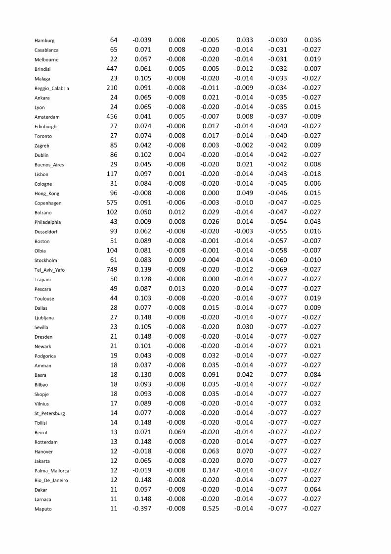
Hamburg 64 -0.039 0.008 -0.005 0.033 -0.030 0.036
Casablanca 65 0.071 0.008 -0.020 -0.014 -0.031 -0.027
Melbourne 22 0.057 -0.008 -0.020 -0.014 -0.031 0.019
Brindisi 447 0.061 -0.005 -0.005 -0.012 -0.032 -0.007
Malaga 23 0.105 -0.008 -0.020 -0.014 -0.033 -0.027
Reggio_Calabria 210 0.091 -0.008 -0.011 -0.009 -0.034 -0.027
Ankara 24 0.065 -0.008 0.021 -0.014 -0.035 -0.027
Lyon 24 0.065 -0.008 -0.020 -0.014 -0.035 0.015
Amsterdam 456 0.041 0.005 -0.007 0.008 -0.037 -0.009
Edinburgh 27 0.074 -0.008 0.017 -0.014 -0.040 -0.027
Toronto 27 0.074 -0.008 0.017 -0.014 -0.040 -0.027
Zagreb 85 0.042 -0.008 0.003 -0.002 -0.042 0.009
Dublin 86 0.102 0.004 -0.020 -0.014 -0.042 -0.027
Buenos_Aires 29 0.045 -0.008 -0.020 0.021 -0.042 0.008
Lisbon 117 0.097 0.001 -0.020 -0.014 -0.043 -0.018
Cologne 31 0.084 -0.008 -0.020 -0.014 -0.045 0.006
Hong_Kong 96 -0.008 -0.008 0.000 0.049 -0.046 0.015
Copenhagen 575 0.091 -0.006 -0.003 -0.010 -0.047 -0.025
Bolzano 102 0.050 0.012 0.029 -0.014 -0.047 -0.027
Philadelphia 43 0.009 -0.008 0.026 -0.014 -0.054 0.043
Dusseldorf 93 0.062 -0.008 -0.020 -0.003 -0.055 0.016
Boston 51 0.089 -0.008 -0.001 -0.014 -0.057 -0.007
Olbia 104 0.081 -0.008 -0.001 -0.014 -0.058 -0.007
Stockholm 61 0.083 0.009 -0.004 -0.014 -0.060 -0.010
Tel_Aviv_Yafo 749 0.139 -0.008 -0.020 -0.012 -0.069 -0.027
Trapani 50 0.128 -0.008 0.000 -0.014 -0.077 -0.027
Pescara 49 0.087 0.013 0.020 -0.014 -0.077 -0.027
Toulouse 44 0.103 -0.008 -0.020 -0.014 -0.077 0.019
Dallas 28 0.077 -0.008 0.015 -0.014 -0.077 0.009
Ljubljana 27 0.148 -0.008 -0.020 -0.014 -0.077 -0.027
Sevilla 23 0.105 -0.008 -0.020 0.030 -0.077 -0.027
Dresden 21 0.148 -0.008 -0.020 -0.014 -0.077 -0.027
Newark 21 0.101 -0.008 -0.020 -0.014 -0.077 0.021
Podgorica 19 0.043 -0.008 0.032 -0.014 -0.077 -0.027
Amman 18 0.037 -0.008 0.035 -0.014 -0.077 -0.027
Basra 18 -0.130 -0.008 0.091 0.042 -0.077 0.084
Bilbao 18 0.093 -0.008 0.035 -0.014 -0.077 -0.027
Skopje 18 0.093 -0.008 0.035 -0.014 -0.077 -0.027
Vilnius 17 0.089 -0.008 -0.020 -0.014 -0.077 0.032
St_Petersburg 14 0.077 -0.008 -0.020 -0.014 -0.077 -0.027
Tbilisi 14 0.148 -0.008 -0.020 -0.014 -0.077 -0.027
Beirut 13 0.071 0.069 -0.020 -0.014 -0.077 -0.027
Rotterdam 13 0.148 -0.008 -0.020 -0.014 -0.077 -0.027
Hanover 12 -0.018 -0.008 0.063 0.070 -0.077 -0.027
Jakarta 12 0.065 -0.008 -0.020 0.070 -0.077 -0.027
Palma_Mallorca 12 -0.019 -0.008 0.147 -0.014 -0.077 -0.027
Rio_De_Janeiro 12 0.148 -0.008 -0.020 -0.014 -0.077 -0.027
Dakar 11 0.057 -0.008 -0.020 -0.014 -0.077 0.064
Larnaca 11 0.148 -0.008 -0.020 -0.014 -0.077 -0.027
Maputo 11 -0.397 -0.008 0.525 -0.014 -0.077 -0.027

Atlanta 10 0.048 -0.008 -0.020 -0.014 -0.077 0.073
Gothenburg 10 0.148 -0.008 -0.020 -0.014 -0.077 -0.027

3.5#1 105
The selected and aggregated candidate explanatory variables are the follow-ing:
Table 3.27: Specified independent variables

Variable Levels
Age -34
35 - 44
45 - 54
55 -
Professional Status in Army
Not in Army
Sex Male
Female
Type of Itinerary Round Trip
One Way
Target_Buy Contract Yes
No
Class Economy, Business, PremiumEconomy
First
Type of Client Corporate
Public Administration
Bank
Type of Flight National
International, Intercontinental
Day of Issuance Weekend
Working days
Day of Departure Weekend
Working days
Day of Return Weekend
Working days
Number of Routes 1
2
3
4 and more
Route FCO_GOA_FCO
FCO_LIN_FCO
FCO_TLV_FCO
LIN_FCO_LIN
OtherRoute
Airline AIR_FRANCE
ALITALIA_CAI_SPA
EASYJET
Other
Distance KM
Advance Booking Days
Table 27: final candidate Explanatory Variables

Distanza_KM
AnticipoPrenotazioneG
AIRLINE

108 3.#1

Chapter 4
Modelling the risk of non-fly
4.1 Simplifying the business problem
The research problem that the TMC explicitly required to address is to cal-culate the probability that a ticket is not flown and, in particular, that itis, either partially or totally, changed or refunded. But this problem is notas easy as it appears at a first sight. In fact, once bought an air ticket, thebusiness traveler can:
1. depart,
2. waive the flight completely, without refund,
3. waive the flight completely, with total refund,
4. fly only a part of the routes included in the ticket and ask refund forthe remaining,
5. entirely change the ticket (for getting a new date and/or new routes),
6. fly only a part of the routes included in the ticket and change theremaining (dates and/or routes).
But, if the traveler changes the ticket, partially or totally, then he can again:
109

110 4.#1
1. depart,
2. waive the flight completely, without refund,
3. waive the flight completely, with total refund,
4. fly only a part of the routes included in the ticket and ask refund forthe remaining,
5. entirely change the ticket (for getting a new date and/or new routes),
6. fly only a part of the routes included in the ticket and change theremaining (dates and/or routes).
And if the traveler changes the ticket, totally or partially, a second time,then he has again the 6 options listed above. Considering that a businesstraveler can potentially change ticket an in(de)finite number of times, thetheoretical dimension of this problem is virtually infinite. Therefore a firstdifficulty consists in simplify the business problem in a way that is logicallyconsistent, economically meaningful, computationally feasible and suitableto reflect the impact of each ticket outcome on the TMC’s business.
It is clear that tickets’ outcomes result from business travelers’ choices,listed above. Namely, a ticket can display one of the following outcomes:
1. flown,
2. not flown,
3. total refund,
4. partial refund,
5. total change,
6. partial change.
And if the ticket is partially changed:

4.1#1 111
• 1 partial change and flown,
• 1 partial change and not flown,
• 1 partial change and total refund,
• 1 partial change and partial refund,
• 1 partial change and 1 total change,
• 2 partial changes.
And similarly, if the ticket is totally changed. Again, each time a ticket ischanged, all the above 6 outcomes are possible. It is to be noted that out-comes cannot be aggregated based neither on their final state, nor on theirinitial state, nor on any intermediate state. In fact, there is a great difference,from both a statistical and an economic perspective, between the apparentlysame outcome at subsequent ’levels’ (so to say: it is possible to consider the6 possible outputs of the first issued ticket as belonging to the first level, the6 possible outputs of the second issued ticket, due to a change, as belongingto the second level, and so forth).
For example, the first-level outcome ’total refund’ differs from asecond-level ’total refund’ because, from the statistical point of view, the ’tra-jectory’ of the first one is ’issuance - total refund’, thus the ticket underwenta single transition between the initial state and the absorbing state. Whilethe trajectory of the second one is, for example, ’issuance - partial change -total refund’, so the ticket passed from the initial state to an intermediatestate, then to the absorbing state, realizing 2 distinct transitions. Indeed,a second-level ’total refund’ also differs from the other possible second-level’total refund’, which would have trajectory: ’issuance - total change - totalrefund’, as the intermediate state differs, though the number of transitions,the final and the absorbing states are the same.
The difference between the mentioned outcomes, in economic terms,is more complicated, because:
112 4.#1
• Seneca stipulates personalized contracts with its clients, so there arenearly as many different economic conditions, producing different eco-nomic outputs for each ticket outcome, as client companies.
• Different airlines offer different conditions, with reference to the oner-ousness of changes and possibility of refund, through different fares andtickets.
The economic difference between ’equal’ tickets outcomes at differentlevels depends on both the conditions applied to clients by Seneca and theconditions applied to Seneca by airlines, which vary with the degree offlexibility of the ticket.
For example, imagine that a client company stipulated a TargetBuy contract with the TMC, providing that it always pays 100 euros forflying in economy class from Rome to Brussels, plus a brokerage commissionequal to 15 euros for each fight and a penalty of 10 euros for each change.Then, hypothesize that the client requests 2 tickets for the specified route,paying a total amount of 230 euros. Let Seneca purchase, on behalf ofthat client, 2 tickets priced 60 euros each, the degree of flexibility of whichcorresponds to the possibility of change with a penalty of 20 euros and thepossibility of refund up to 50% of the price. If the outcome of one ticket isfirst-level ’total refund’, then the economic output, for the TMC, is equalto: 100 + 15− 60− 100 + 30 = −15 euros, while, if the outcome of the otherticket is second-level ’total refund’, then the economic output, for the TMC,equals: 100 + 15− 60 + 10− 20− 100 + 30 = −25 euros.
A further example. Imagine that the Target Buy contract, for sameclient company, provides also that it always pays 1,000 euros for flyingfrom Brussels to New York, with a penalty of 250 euros for each change.The client requires 2 tickets to reach Brussels from Rome, then New Yorkfrom Brussels. Seneca buys, on behalf of that client, 2 non-refundabletickets, covering both routes, priced 500 euros, with a penalty of 70

4.1#1 113
euro in case of change. Then, one ticket is first totally changed, thentotally refunded, producing an economic result, for the TMC, equal to:100 + 1, 000 + 15 − 500 + 250 + 10 − 70 − 1, 100 = −295 euros. Withreference to the other ticket, the client asks to anticipate the date of theflight from Rome to Brussels, leaving the flight from Brussels to NewYork unchanged (partial change). But, just a few days before the date ofdeparture, the business traveler has a hitch impeding him to do the journey,so he asks the total refund. Thus, the economic output of the transaction is:100 + 1, 000 + 15− 500 + 10− 70− 1, 100 = −545 euros.
As shown in the above examples, the economic result of each transac-tion, for Seneca, depends on a lot of factors, most of them out of its control,but the more numerous the changes, the more probable that the TMCattains a bigger loss. And, of course, if the client company asks the refund,it is more probable that the economic result is negative, compared to thesituation in which the refund is not required. It is also evident that a moreexpensive and flexible ticket is convenient in case of changes and/or refund,whence the importance of estimating the probability of each outcome of theticket.
As there is no literature helping in the specification of the dependentvariable(s), different options have been explored, based on the sample distri-bution and on the information collected through the qualitative investigationof the context. Finally, the following tree specification, reflecting both thelogical and the dynamic structure of the business travelers’ decision-makingprocess, has been selected:
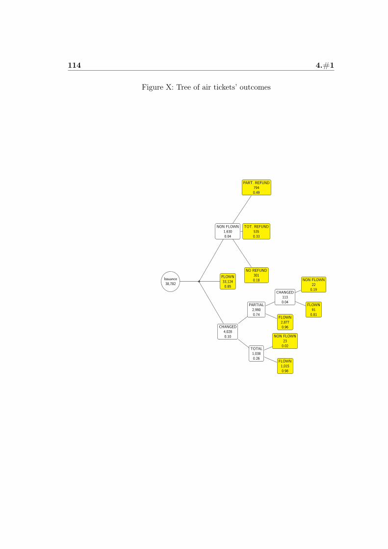
114 4.#1
Figure X: Tree of air tickets’ outcomes
Issuance38,782
CHANGED4,0280.10
TOTAL1,0380.26
FLOWN1,0150.98
NON FLOWN230.02
PARTIAL2,9900.74
FLOWN2,8770.96
CHANGED1130.04
FLOWN910.81
NON FLOWN220.19
FLOWN33,1240.85
NON FLOWN1,6300.04
NO REFUND3010.18
TOT. REFUND5350.33
PART. REFUND7940.49

4.1#1 115
The leaves of the tree, colored in yellow, represent the absorbing statesof the tickets. The observed tickets for which the outcome is non-missingare 38,782, the missing data are indeed right-censored, as the departuredate was posterior to that of the data collection and no change nor refundwas required up to that time. Censored data are excluded from estimationsample and subsequently included in the forecasting one, where the fulltrajectory of those tickets will be recorded. The formalization shown inthe tree allows to simplify the problem, assuming that it is composed by 6variables:
• Y 1 is a trinomial variable, which can assume the modalities: Flown,Non Flown, Changed;
• Y 2 | Y 1 = NONflown is a trinomial variable, which can assume themodalities: No Refund, Total Refund, Partial Refund;
• Y 3 | Y 1 = Changed is a binary variable, which can assume the modal-ities: Totally changed, Partially changed;
• Y 4 | Y 3 = Totallychanged is a binary variable, which can assume themodalities: (Totally changed and) Flown, (Totally changed and) NonFlown;
• Y 5 | Y 3 = Partiallychanged is a binary variable, which can assumethe modalities: (Partially changed and) Flown, (Partially changed and,again, Partially) Changed;
• Y 6 | Y 5 = Changed is a binary variable, which can assume the modal-ities: (twice Partially changed and) Flown, (twice Partially changedand) Non Flown.
116 4.#1
Such a formalization implies a simplification, allowing to avoid over-parametrization and to specify identified models, if compared with a simul-taneous one, where only a variable is considered, but it would be a nominalvariable, composed by 9 levels (one for each leave), each of which affected byall the relevant explanatory variables.
Conversely, this way a structure of conditional independence relationscan hold, although must be empirically verified. Namely, if X is the vectorof all candidate explanatory variables, ’subsettable’ in J vectors, xj, and ifY 1 depends on x1, then it is possible that Y 2 ⊥ x1 | Y 1 = NonFlown andY 3 ⊥ x1 | Y 1 = Changed. Similarly, if x2 is the set of explanatory variablesfor Y 3, it is possible that Y 4 ⊥ x2 | Y 3 = Total and Y 5 ⊥ x2 | Y 3 = Partial.Finally, if x3 is the set of variables correlated with Y 5, it is possible thatY 6 ⊥ x3 | Y 5 = Changed.
Thus, if no residual effect, of ’grandparents’ variables is empiricallydetected, the loss of efficiency, due to the progressive diminution of the sam-ple size at descending the branches of the tree, is compensated by the minornumber of parameters to be estimated. But the tree formalization of thebusiness problem requires other independence conditions to hold, namelythat:
• the business traveler’s choice of not asking the refund, asking a partialrefund (while flying the rest of routes) or a total one, once he decidednot to fly (the first bought ticket) is independent by the alternatives offlying the ticket or changing it;
• when choosing whether to completely or partially change the (firstbought) ticket, the business traveler does not consider anymore thepossibility of flying it or to waive the flight;
• once totally changed the ticket, the traveler considers only two possiblechoices: to fly it, or not to fly it (changes are included in the latter, butno further modelled, due to scarcity of observations), independently
4.2#1 117
from the possibilities represented by other nodes of the tree;
• once partially changed the ticket, the traveler chooses between changingit again or flying it, independently from any other node of the tree;
• after changing the ticket twice, the traveler decides to leave or notto leave (further changes are included in the latter, but no furthermodelled, due to scarcity of observations), not influenced by any otheralternative.
Thus, such conditions can be called ’irrelevance of higher-level alternatives’,then the discussion on their validity may be included in the well known issueof Independence from Irrelevant Alternatives.
4.2 Models specification
Since the time elapsed between the moment of booking and the departuredate is said, by the TMC’s experts, to be crucial for predicting the tickets’outcomes, a first attempt was made to model it as a stochastic process,representing the ticket trajectory from the first issuance to the final leaf. Buttoo many errors in recording dates made practically impossible to estimateduration models, namely the Proportional Hazard and the Multi-stateMarkov models (see: Florens et al, 2008).
Then, many different classifiers were tried:
• Classification Trees;
• Random Forests;
118 4.#1
• Hierarchica Models;
• Bayesian models.
But no available independent variable resulted useful to subset observationsaccording to a classification tree. Random forests semed to work pretty wellon the training sample, but their performances on the test sample were evenworse thant those discussed in the following chapter. No hierarchical modelis feasible, because the dataset is too unbalanced, the identifiers of groupsare missing in too many cases and it is not sure that an unidentified individ-ual does not belong to an identified group. Bayesian models were consideredbecause of the hope to get some prior information from the experts of theTMC, able to integrate the poor data provided by the corporate dataset.But no further information became available, so that the bayesian approachwould have led to the same results of the frequentist one.
However, the qualitative study of the context and the decision treespecification, describing the phenomenon under investigation as the decision-making process of business travelers, make natural to employ discrete choicemodels. In particular, the MLM resulted the most viable methodologicalchoice, in the present case, especially considering that the various types ofMLM can be derived from the general Random Utility Model (Train, 2009).
Thus, the unknown utility of the j-th ’flying choice’ for the n-th busi-ness traveler, Un,j, is a function Vn,j of the characteristics of the j-th alterna-tive, Sn,j, and of the traveler-specific variables, Zn, plus a random component,εn,j, representing the unobservable elements of Un,j. Unluckily, in the presentcase no information on Vn,j is available, thus:
Un,j = Vn,j + εn,j = Vj(Zn) + εn,j (4.1)

4.2#1 119
As it is logical to assume that the traveler chooses the option yielding thegreater utility, then, if the baseline alternative is the j-th, the probabilitythat the n-th business traveler makes the i-th decision is:
Pn, i = P [Un,i > Un,j] = P [Vn,j+εn,j < Vn,i+εn,i] = P [εn,j−εn,i < Vn,i−Vn,j] =
(4.2)
= Fεn,i−εn,j(Vn,i − Vn,j) =
∫1εn,i−εn,j<Vn,i−Vn,jf(εn)δεn (4.3)
Then, if εn ∼IID Gumbel(µ, γ) and, as in the present case, only thecharacteristics of the decision-maker are available as explanatory variables,the Pure MLN is obtained:
Un,j = Znβj + εn,j (4.4)
f(εn,j) = exp−εn,jexp−exp−εn,j (4.5)
F (εn,j) = exp−exp−εn,j (4.6)
Where each (level of each) explanatory variable has an alternative-specificparameter, βj, and the utility is ’normalized’, so that it has a scale andthe model is basically identified, once set βk = 0 if the k-th categoryis the reference one, thanks to the constant variance of the error term:V ar[εn,j] = π2
6. As the difference of two Gumbel-distributed variables has
Logistic distribution, if ε∗n,j = εn,j − εn,i, then ε∗n,j ∼ Logistic(s,m) and:
F (ε∗n,i) =expε∗n
1 + expε∗n(4.7)
Pn, i = P [εn,j < V n, i+ εn,i − V n, j] = (4.8)

120 4.#1
=
∫ ∏j 6=i
exp−exp−(Znβi+εn,i−Znβj)exp−εn,iexp−exp−εn,iδεn,i =
(4.9)
=expZnβi
1 +∑
j Znβj(4.10)
Generally, the Pure MLM is interpreted in terms of odds: oddi,j =
expZn(βi − βj) so that if δzm is an increment in the m-th explanatoryvariable, then its effect on the probability that the decision-maker choosesthe i-th alternative, over the reference choice, k, equals to:
oddi,k(Zn, zn,m + δzm)
oddi,k(Zn, zn,m)= expβm,iδzm (4.11)
and the marginal effect of zn,m equals δPn,iδzn,m
. The Maximum Likelihood Esti-mate (MLE) of the model is simply, as the log likelihood function is globallyconcave. Its functional form is the following:
L =N∏n=1
(∏j
P1n,jn,j ) (4.12)
ln(L) =N∑n=1
(∑j
1n,jln
(expZnβi∑expZnβj
)(4.13)
where 1n,j is an indicator function, equal to 1 if the n-th business trav-eler chooses alternative j, 0 otherwise. To facilitate the economic interpre-tation of estimated coefficients, usually they are standardized: ˆβj,m,SD =
[expβj,m− 1] ∗ 100, then ˆβj,m,SD equals the percentage variation in the oddratio, produced by a unitary increment of the m-th independent variable.
Whether the random components εn,j are not identically distributed

4.2#1 121
and, in particular, they are heteroskedastic, V ar[εn,j] = σ2j 6= V ar[εn,i] =
σ2i ,∀i 6= j, then the relation between σ2
j and the decision-maker’s character-istics makes the estimates of the Pure MLN coefficients inefficient, biased andinconsistent, and an Heteroskedastic MLM, or Parametrized HeteroskedasticMLM, must be specified. Its form is the following:
Uj,n = Znβj + σjεn,j (4.14)
Such a specification does not need the IIA to hold and allows to model alsodifferent variances for different decision-makers. For simplicity, consideringan only individual, εj ∼ Gumbel(0, σj) and
f(εj) =1
σjexp− εj
σjexp−exp− εj
σj (4.15)
Fεj(z) =
εj=z∫f(εj)δεj = exp−exp− z
σj (4.16)
Then, the probability that the business traveler chooses alternative i is:
Pi = P [εj < zβi + εi − zβj] =
∫ ∏Λzβi + εi − zβj
σj
1
σiλεiσiδεi (4.17)
where Λ and λ are respectively the Gumbel density and the Gumbel cumula-tive function. σi can be interpreted as a measure of the degree of uncertaintyassociated with the expected value of the utility, E[Ui] = zβi , due to theunobservable part of the decision-maker’s utility, εi, thus it can be seen asthe relative weight of the utility’s random component, with respect to itssystematic ones, zβi, for estimating Pi. It also includes the effect of changesin the available set of alternatives, on the probability of choosing each alter-native, in which the violation of IIA consists. Thus, the higher the estimatedvalue of σi, the lower the impact of (zβj)− (zβi) on Pi, the greater the effect
122 4.#1
of εi− εj, the smaller the elasticity effect on Pi. Also this model is estimatedthrough MLE. Comparing the estimates of Pure MLM and HeteroskedasticMLM, including the same variables, is also useful as residuals diagnostics.
Given the tree formalization, presented above, it may be the case thatthe IIA holds between but not within some set of alternatives, namely thosecoded as levels of the same Y n variable. For example, it can be possible that,once decided not to fly, the business traveler’s choice of not asking the refundis influenced by the possibilities of asking a total refund or asking a partialrefund, but not by those of changing the ticket partially or totally. In sucha case, each Y n variable can be seen as the s-th cluster of levels of a singlevariable, including all the nodes of the tree, so that alternatives within eachcluster are correlated, but they are independent from alternatives in otherclusters. Then, a Nested MLM should be specified:
Un,j = Znβj + εn,j,s (4.18)
where V ar[εn,j,s] = σ2s = V ar[εn,i,s], ∀j, i ∈ Nests;V ar[εn,j,s] = σ2
s 6=V ar[εn,k,l] = σ2
l ,∀j ∈ Nests, k ∈ Nestl, i.e. the error variance is constantwithin each nest, but can differ between nests. Then, the actual probabilityof choosing alternative j is the joint probability of selecting an alternativewithin Nests and of selecting alternative j between all the alternatives inNests:
P [j,Nests] = P [Nests]P [J | Nests] (4.19)
Therefore, the Nested MLM is composed by a two levels specification, plusa connecting term:
P [Nests] =expZnβj + λsIVn,s∑
∀NesthexpZnβi + λhIVn,h
(4.20)
4.3#1 123
P [J | Nests] =expZnβj
λs∑
i∈NestsexpZnβi
λs
(4.21)
IVn,s = ln
( ∑j∈Nests
expZnβjλs)
(4.22)
Where IVn,s is the so-called Inclusive Value, representing the ex-pected utility, for the n-th business traveler, of chosing the Nests,E[Un,s] = E[maxj∈Nests(Znβj + εn,j)] and λ ∈ [0, 1]. Also this model can beestimated through MLE. All the 3 descripted models are considered in thesearch for a specification for the risk of non-fly.
4.3 Notes on the Independence from Irrelevant Alter-
natives
For a MLM to be correctly specified, it is necessary that all the followingassumptions hold:
• with reference to their outcome, the n tickets can be considered n in-dependent trials, happening in equal conditions;
• each outcome is not (necessarily) independent from the others;
• the probability of each outcome is constant in each trial;
• the listed tickets’ outcomes are both exhaustive and mutually exclusive;
• the Independence from/of the Irrelevant Alternatives (IIA)
While the second hypothesis is especially convenient for the present case,in general, it is likely that both the independence and the ’constancy’assumptions hold conditionally to the explanatory variables, if the latter

124 4.#1
are actually able to synthesize the business and environmental factorsdetermining the travelers’ behavior. Also the fourth assumption should holdin the present case, with the limits mentioned above (concerning the virtualinfinity of possible outputs). Conversely, the IIA deserves a dedicateddiscussion, because, if the IIA is violated, then the Maximum LikelihoodEstimates (MLE) of the model’s parameters are biased and vary with theconsidered set of alternatives - of tickets’ outcomes, in the present case -(McFadden et al, 1978). There are 3 main formulations of IIA, which arenot equivalent when individual preference ordering are aggregated throughthe rank-order method, to obtain a social choice function - a consistentsample distribution, in the present case - (Ray, 1973).
The easiest formulation of IIA is that by Radner and Marschak(1954), which, applied to the present work, results to be the follow-ing. Let T be the (infinite) set of all the possible tickets outcomes, yt,t = 1, ... + ∞, and S the finite subset of T, which it is considered andmodelled in this study. yj ∈ S ⊂ T , j = 1, ..., 9. Let C be a choicefunction, defined on the set of the alternative outcomes, then IIA statesthat if yj ∈ Img(C(T )) ⇒ yj ∈ Img(C(S)). In other words, for IIA tohold it is necessary that the business travelers exhibit a particular behavior(generating yj), independently on the other elements of the set of alternativebehaviors they could assume, whether the set was more or less numerous.For example, IIA requires that, if a traveler needs to partially change thereserved ticket, e.g. because his travel aims at meeting 2 clients in 2 differentplaces, 1 of which is no more available for the reserved date, he will changeit partially (so that he will fly and meet the available client, but not theunavailable one), independently on whether or not the option of, e.g., partialrefund is available (as getting the refund instead of the partial change wouldnot allow him to reach the other client in a new date).
The most known formulation of IIA is surely that of Arrow (1963),which, in the present situation, can be recalled this way. Let ∗ and #

4.3#1 125
denote 2 different business travelers, with individual preferences ordering:y∗j1, ..., y∗j9 and y#
j1, ..., y#j9. Let C∗(S) and C#(S) be the two travelers’
choice/utility functions defined on S, the set of alternatives including yj. LetA and B be 2 alternatives available to the two business travelers: A,B ∈ S,then, according to IIA, for each possible ticket outcome (or equivalentlytravelr’s possible choice) J, Ay∗jB ∧ Ay#
j B ⇔ C∗(S) = C#(S). In otherwords, according to both travelers alternative A is the preferred one andalternative B is the least desired one, independently on all the other possiblealternatives, if and only if their utility functions, defined on the set ofavailable choices, are the same. So, for IIA to hold it is necessary to admitthat, for example, 2 business travelers prefer to totally change the ticket fora flight on Friday and their least desired option is that of flying the ticketon Friday, independently on the fact that they could or could not changethe ticket only partially or ask the refund or not fly at all, because, e.g.,their utility function is the same, as they want to spend the weekend withtheir family, while not giving up the travel.
Finally, the probabilistic formulation of IIA is that of Luce (1958),which, in the present case, can be viewed as follows. Let Ps(A) indi-cate the probability of choosing alternative A among the elements of S,and P (A/B) denotes the probability of choosing alternative A amongA and B. For each couple of alternatives A,B ∈ S ⊂ T < +∞, ifP (A/B) 6= 0 ⇒ P (A/B)
P (B/A)= Ps(A)
Ps(B). And, if IIA holds, then Ps(A)
Ps(B)= P (A)
P (B). In
other words, for IIA to be valid, the probability of each decision of businesstravelers, choosing among two different alternatives, must be independenton all the other available alternatives. So, for example, IIA requires that ifthe odd of fly is 0.8, then it stays equal to 0.8 whether the only alternativefor the business traveler is that of not fly, whether he can also choose tochange the ticket partially, whether he can also change it totally and soforth.
The formalization of Luce (1958) leads directly to understand the

126 4.#1
importance of IIA for MLM: in the MLM any category can indifferentlybe considered as the base in the logit transformation, as it is alwayspossible to convert the ratio from one formulation to another, providedthat the odd between two alternatives is invariant to the introduction ordeletion of other alternatives in the considered set. I.e: if k, l,m ∈ S
and xk, xl, xm are the characteristics of the corresponding choice, while sis the vector of the business traveler’s characteristics, then IIA is valid⇔ P (k|S)
P (m|S)= expC(xk,s)
expC(xm,s) ⇒ P (k/m) ⊥ l|S.Although, considering the previous examples and the fact that
business travelers’ choices are not arbitrary, but led by working motiva-tions mainly independent on their own will, the circumstance that thephenomenon under investigation should theoretically comply with IIArequirements does not guarantee that IIA is effectively valid in the MLMwhich can be employed. In fact, as highlighted by McFadden et al. (1981),violations of IIA do not concern the structure of the choices themselves, butthe particular specification of the used model. Thus, for any set of choices,for any phenomenon, IIA can hold for one specification of the explanatoryvariables, but not for another one. Indeed, violations of IIA can be seen asa specific kind of omitted variable bias, as this property holds only if theomitted variables are independent and random.
Whence the difficulty of knowing a priori whether the MLM can becorrectly used, as the omitted variables are absent because they are notobserved. Of course, it is possible to hypothesize those omitted variables,their relations and their influences on the variables of interest, according tothe available knowledge of the context of the study. But there is no wayto ascertain a priori that such a guess is indeed correct and that no otheromitted variable affects the choice. While, for an ex-post verification of IIA,various tests have been developed.
There are two types of statistical tests for IIA. The first one is veryintuitive, it is the easiest to implement and consists in estimating MLM on

4.3#1 127
different subsets (and also on the full set) of the possible alternatives, amongwhich the choice is made. Then the parameters of the estimated models arecompared and, if they are not significantly different, IIA is verified to hold.The most popular tests of this kind are: Hausmann-McFadden’s test ofmisspecification (1984), and McFadden-Train-Tye’s test (1981), Horowitz’stest (1981) and Small-Hisiao’s test (1985), which are all variants of theLikelihood Ratio test. Unfortunately, those tests, relying on asymptotictheory, have very disappointing finite sample properties. In particular, thesizes of these tests are affected by serious distorsions (Cheng and Long,2007) and their power is substantially too low to make them reliable (Fryand Harris, 1996).
The second type of statistical tests for IIA is model-based. It consistsin estimating more general models, not requiring the IIA property, thentesting the constraints on parameters to zero, which reconduct the models tothe bond of IIA. Such general models, which also constitute an alternativeto MLM whenever IIA does not hold, are: DOGIT (Gaudry and Dagenais,1979), Multinomial Probit, Nested Logit and Mixed Logit (Train, 2003).The constraints on parameters can be tested through the usual Wald test,Likelyhood Ratio test and Lagrange Multiplier (LM) score test (in theformulation of Tse, 1987). The finite sample properties of 2 tests of thiskind, namely the LM and its extension by King and Wu (1993): the LocallyMost Mean Powerful (LMMP) test, were investigated by Fry and Harris(1996) throug a Monte Carlo study. They found that the empirical size ofLM is far below the nominal one for any sample size, but also the LMMPtest is affected by undersize distorsion, leading to over-accptance of the nullhypothesis of IIA. Nonetheless, their power is more satisfying, and their sizedistorsion less serious than that of the tests based on the partitioning ofthe choice set. However, the main problem with this kind of tests is thatof identification, as the more general is the model, the more numerous arethe parameters to be estimated, the number of which, moreover, affects the
128 4.#1
power of the test.Though the problem of verifying IIA seems irresolvable, McFadden et
al (1978) made an encouraging consideration: whenever IIA does not hold,the usual residuals diagnostics and goodness-of-fit tests highlight that thereis a problem of misspecification. Therefore, it can be assumed that if theresiduals are well behaved, the model fits well and the qualitative knowledgeof the context leads to hypothesize that IIA can hold, then it is very likelythat it actually holds.
4.4 Variables selection
Whenever, as in the present work, there is no literature guiding the modelspecification, any specification search procedure must be necessarily data-driven, implying some difficulties. First, from a theoretical perspective, thecontingency, fortuity chatacter of the relations between variables, portrayedby the obtained model. As any sample is somehow randomly selected, thecorrelations found in sample may not apply to other samples of the referencepopulation, nor to the latter. Whether it is the case, the selected specifica-tion, missing some important predictors or including some unrelevant ones,describes only the sample, thus the knowledge retrieved from the data is notextensible to the population, and, more important to this work, the modelis not able to reliably predict out of sample realizations of the phenomenonof interest. The cause of the sample non-representativeness is essentially aselection bias.
For the present work there was not a real sampling procedure: withreference to the cross-sectional dimension, the whole population of air ticketsintermediated by Seneca is observed, but with respect to the time dimension,the dataset covers only a small temporal interval. Therefore, a model selectedbased on the available dataset could display a poor forecasting performance
4.4#1 129
due to 2 sources of selection bias. First, the eventual difference in businesstravelers’ behavior in different periods of the year (as just some moth of ob-servation are available) and in different years (e.g. it may be the case thatin a certain year an exibition, a war, an epidemic caused a modification oftheir propensity to change or waive the flights). Second, as there are somemissing data, the eventual difference in proportions of clients and ticketswith certain modalities of the explanatory variables, between the observedand the unobserved realizations of the ’non-fly phenomenon’. While the biasinduced by the latter can be tested, as it is done in the chapter dedicated tothe description of the data, and eventually corrected through weights, thereis no way to quantify or avoid the bias due to the small time window.
A second problem with data-driven specification search is that, sub-stantially, the only feasible practices are forward and backward stepwiseprocedures, eventually combined. Indeed, in the present case, a backwardstepwise is unviable, due to the limited degrees of freedom available. Butthe use of stepwise procedures is greatly discouraged, because the selectedexplanatory variables can be non-significant, although with small P-values,and the excluded ones can be important predictors, though their P-valuesappear over the (arbitrarily) set acceptance threshold (Harrell, 2001).
Freedman (1983) showed the paradoxical results obtainable throughthese methods: he generated independent normal variables, applied stepwiseand found significant correlations between them. Many other researches con-firmed that stepwise techniques lead to the selection of models with a smallnumber (if compared to that of all the actually significant regressors) of ex-planatory variables, with highly significant coefficients and inflated values ofR-squared and R-squared-like statistics, even though covariates are not evenminimally correlated with the dependent variable, when the number of can-didate regressors is very close to the size of the estimation sample (Lukacs etal., 2010; Flom and Cassell, 2007; Foster and Stine, 2006).
This so called ’Freedman Paradox’ is due to the downward biasedness
130 4.#1
of standard errors of regression coefficients, producing too narrow confidenceintervals, estimates biased in absolute value and too small p-values for theselected model, which will then show a poor forecasting performance (Shat-land et al., 2008). Moreover, the selection is usually unstable, sensitive tosmall perturbations in the data: adding or deleting a small number of obser-vations, the model resulting to be the ’best’ one can change (Steyerberg etal, 2000).
In particular, when the aim is obtaining a reliable predictor, the mainproblem is the "agonizing process of choosing the ’right’ critical p-value instepwise regression" (Shatland et al., 2008, p. 2). Many authors suggest tokeep all the candidate regressors, or to set a high acceptance threshold (e.g.p-values of 0.5, see: Harrell, 2001; Steyerberg et al, 2000; Steyerberg et al,2001), but if the problem is the scarcity of degrees of freedom, this option islikely to be unviable.
Although many researchers conclude that stepwise should be com-pletely avoided, in practice it is necessary, in absence of an economic the-ory, as in the present case. Thus, a forward stepwise is employed for themodel selection, but cautiously taking into account all the mentioned issues.Moreover, here stepwise is only the first step of the predictive specificationsearch, it is not done automatically and some useful shrewdness are addedto the standard procedure. In particular, if K is the number of all availablecandidate explanatory variables and k is the number of those entering a sin-gle model, in the case of the MLM, the iterative procedure is composed byJ ≤ K − 1 iterations, each consiting in the followinf steps.
1. For j = 0, 1, ..., J , the j-th iteration starts estimating 3∗(K−j) modelswith k = j + 1: a Pure MLM, an Heteroskedastic MLN and a NestedMLM, for each of the K− j candidate regressors (since iteration 1, thisis done augmenting b(j−1) specification - see the following - with theremaining candidate regressors).

4.4#1 131
2. Within each triplet, the 3 different specifications, including the sameregressor(s), are compare in terms of log-likelihood value, McFadden R-squared and likelihood ratio test, to find an eventual correctly specifiedmodel. In fact, such a comparison has also a diagnostic function: ifPure MLN is the ’best’ one, residuals are homoskedastic and IIA holds;if Nested MLM is to be preferred, IIA holds only within ’clusters’ ofalternatives; if Heteroskedastic MLM is the most sound, residuals areheteroskedastic and IIA does not hold.
3. All the correctly specified models, with all the coefficients’ p-values mi-nor or equal to 0.3 are included in the bouquet of ’best’ specifications(the 0.3 threshold is fixed on empirical basis, to obtain a manage-able number of ’best’ models, while including at least an explanatoryvariable for the last branches of the tree, as it is necessary to makepredictions).
4. Among these models, the best specification bj is selected, again basedon log-likelihood value, McFadden R-squared and likelihood ratio test.
5. Steps 1-4 are iterated until no candidate regressor remains, or it doesno entry bj with a significant coefficient.
Thus, the output of this specification search procedure is not a single model,but rather a bouquet of models, found along a single trajectory b in thespace of all the possible specifications. In practice, the ’pure’ stepwise wasemployed only for reducing the cardinality of the models space, equal to6K , to the manageable number of 3K. The selected models should correctlydescribe the relations between variables, a first check of it consists inverifying that the coefficients for the same independent variable display thesame sign and not too different values in different, nested estimated models.Afterwards obtained models must be validated, in order to both exclude thebias, which could be present due to the use of (though a more sofisticated)
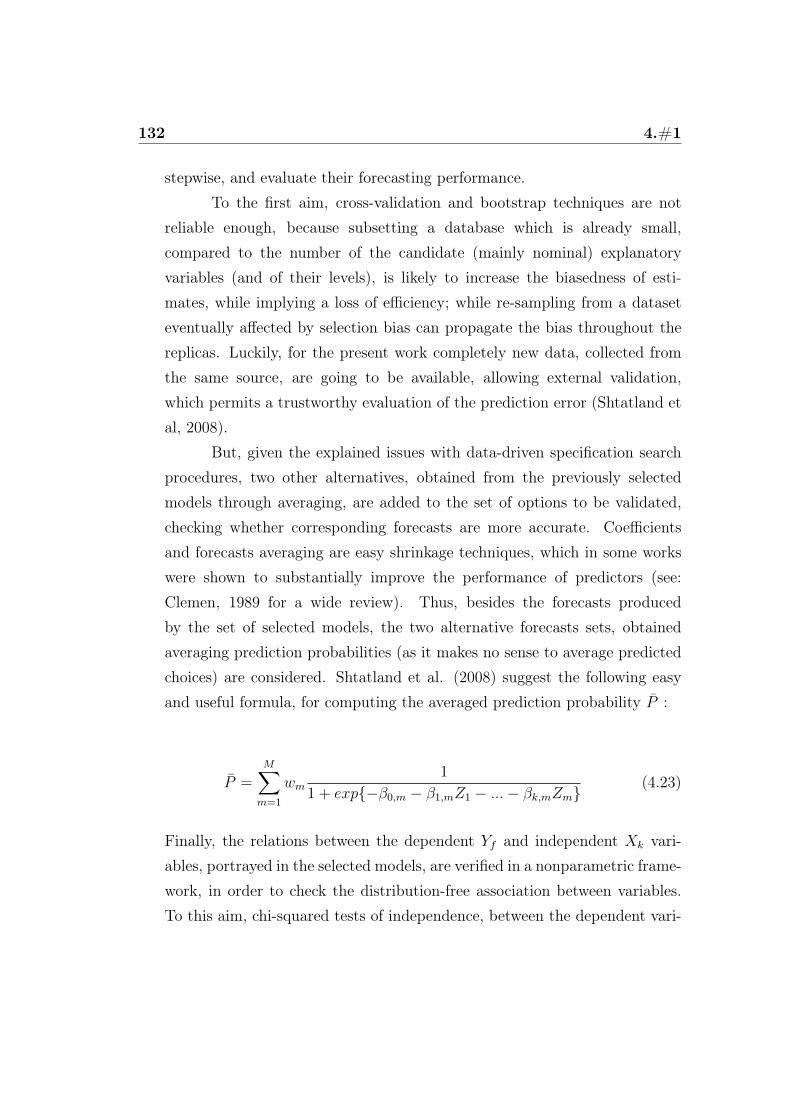
132 4.#1
stepwise, and evaluate their forecasting performance.To the first aim, cross-validation and bootstrap techniques are not
reliable enough, because subsetting a database which is already small,compared to the number of the candidate (mainly nominal) explanatoryvariables (and of their levels), is likely to increase the biasedness of esti-mates, while implying a loss of efficiency; while re-sampling from a dataseteventually affected by selection bias can propagate the bias throughout thereplicas. Luckily, for the present work completely new data, collected fromthe same source, are going to be available, allowing external validation,which permits a trustworthy evaluation of the prediction error (Shtatland etal, 2008).
But, given the explained issues with data-driven specification searchprocedures, two other alternatives, obtained from the previously selectedmodels through averaging, are added to the set of options to be validated,checking whether corresponding forecasts are more accurate. Coefficientsand forecasts averaging are easy shrinkage techniques, which in some workswere shown to substantially improve the performance of predictors (see:Clemen, 1989 for a wide review). Thus, besides the forecasts producedby the set of selected models, the two alternative forecasts sets, obtainedaveraging prediction probabilities (as it makes no sense to average predictedchoices) are considered. Shtatland et al. (2008) suggest the following easyand useful formula, for computing the averaged prediction probability P :
P =M∑m=1
wm1
1 + exp−β0,m − β1,mZ1 − ...− βk,mZm(4.23)
Finally, the relations between the dependent Yf and independent Xk vari-ables, portrayed in the selected models, are verified in a nonparametric frame-work, in order to check the distribution-free association between variables.To this aim, chi-squared tests of independence, between the dependent vari-
4.4#1 133
ables and each candidate explanatory variable, are performed.This method is chosen because the resulting P-values are measures
of association comparable across different variables, of various nature (nom-inal, ordinal, continuous, which are temporarily discretized in classes) andsupport. For each dependent variable, a nonparametric selection of explana-tory ones, parallel to the forward stepwise procedure, is realized as follows.Let K be the number of candidate explanatory variables and S the numberof those which will be selected in the end.
1. The independence of Yf and Xk, ∀k = 1, ..., K is tested.
2. The variable for which the P-value is the lowest, X∗s , is selected assignificantly related with Yf .
3. The independence of Yf and Xk, ∀k = 1, ..., K − s, conditional to X∗s ,is tested.
Steps 2 and 3 are iterated S ≤ K times, until no further variable significantlyrelated to the dependent one, conditional to all the previously selectedvariables, is found.
Although such a procedure is implemented in order to seek confir-mation of the results of the parametric variables selection, it too is not freefrom problems. In fact, it suffers from the gradual loss of efficiency, due tothe progressive shrinking of the sample, necessary to test the relations ofconditional independence. Therefore, it can happen that variables ’truly’highly associated are not selected, because in some shrunk samples notall of their levels are observed, at worst all the tickets display the samevalue. Therefore, the chi-square based procedure tends to underestimate thenumber of significant explanatory variables.

134 4.#1
4.5 Estimations resuts
As already mentioned, the business traveler is identified in 25,749 cases in theestimation sample and just in 7,506 cases in the forecasting sample, thereforethe variables selection procedure described above is repeated on this sub-sample of the estimation sample, in order to avoid favouring the inclusion ofthe variables with less missing data (model estimated on this subsample aremarked with "a").
Moreover, variables sex and age of the traveler are recorded just in2,432 cases in the estimation sample and in 1,868 cases in the forecastingsample, thus the variables selection is repeated once more on this subsample,but only for descriptive purposes (model estimated on this subset of data aremarked with "b").
With reference to the residuals diagnostic, the Pure MLM is the bestfitting specification, between the 3 discrete choice models considered, so theassumptions of homoskedasticity and non-correlated alternatives hold. Signsand values of different estimates for coefficients referring to the same vari-able are consistent and stable throughout models. But the goodness of fitmeasures are very disappointing, highlighting the very low correlation withthe dependent variable and the definitely insufficient explanatory power ofavailable independent variables. The full outputs for the bundle of selectedmodels is available upon request.
Regrettably, also the comparison between the chi-square based vari-ables selection and the results of the stepwise based procedure, shown below,are not encouraging.
Table 4.1: Comparison of parametric and non-parametric variables selectionsresults
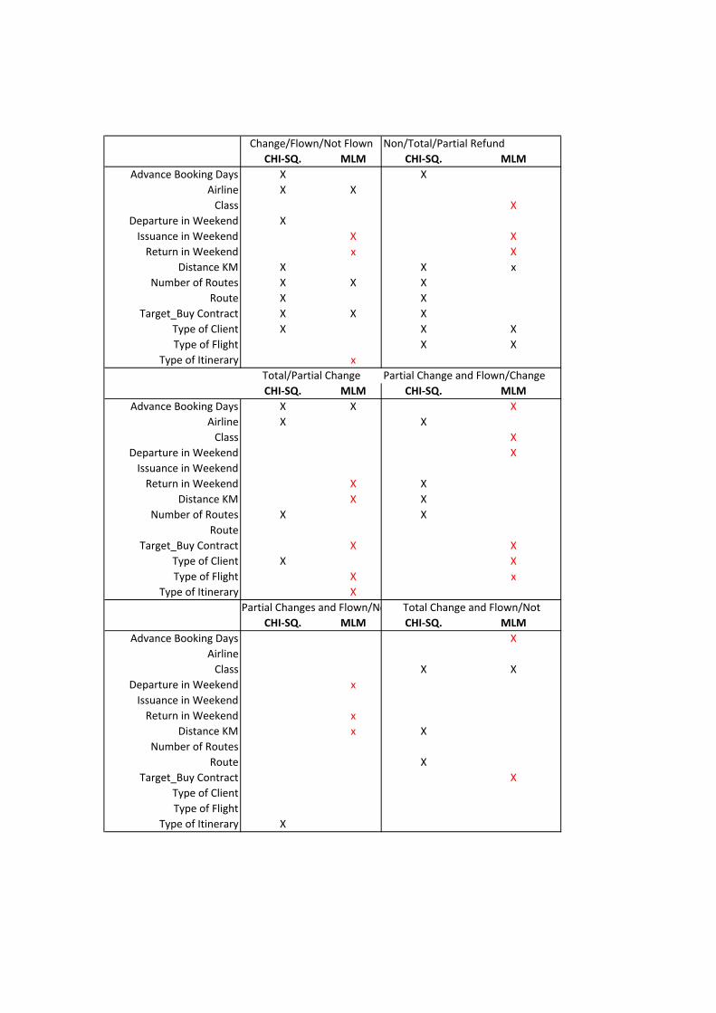
Non/Total/Partial RefundCHI-SQ. MLM CHI-SQ. MLM
Advance Booking Days X XAirline X X
Class XDeparture in Weekend X
Issuance in Weekend X XReturn in Weekend x X
Distance KM X X xNumber of Routes X X X
Route X XTarget_Buy Contract X X X
Type of Client X X XType of Flight X X
Type of Itinerary xPartial Change and Flown/Change
CHI-SQ. MLM CHI-SQ. MLMAdvance Booking Days X X X
Airline X XClass X
Departure in Weekend XIssuance in Weekend
Return in Weekend X XDistance KM X X
Number of Routes X XRoute
Target_Buy Contract X XType of Client X XType of Flight X x
Type of Itinerary X
CHI-SQ. MLM CHI-SQ. MLMAdvance Booking Days X
AirlineClass X X
Departure in Weekend xIssuance in Weekend
Return in Weekend xDistance KM x X
Number of RoutesRoute X
Target_Buy Contract XType of ClientType of Flight
Type of Itinerary X
2 Partial Changes and Flown/Not Total Change and Flown/Not
Change/Flown/Not Flown
Total/Partial Change

136 4.#1
Red crosses indicate that the corresponding variable is selected in MLMbut not in Chi-square selection. The reason of concern is not only theinconsistency of most of selected/dropped variables, but also the fact thatthe non-parametric method is expected to select less variables than thewhole set of actually significant regressors, while here it includes morevariables than the stepwise procedure for MLM. This evidence confirmsthat the available information is insufficient to effectively model the phe-nomenon under investigation, thus results must be read very cautiously.
Estimation results indicate that the smaller the number of routes,the higher the propensity, of the business traveler, to fly the first purchasedticket, while if the flight covers 5 routes or more, it is more likely that thefirst ticket is not flown. An eventual ’speculative’ behavior of Target-Buyclients is not supported by estimates, in fact the probability that a clientwith this type of contract flies the first ticket is slightly higher than theone that he changes or waivers the flight. A higher positive effect on thepropensity to fly is found for the variable indicating that the first ticket wasissued during the weekend. This evidence suggests that tickets reserved inthe weekend, when business traveler should not work, are for ’emergencies’and, as such, they are normally flown.
When the flight is provided by Alitalia and Easy Jet the probabilitythat it is flown are higher that those for (other) low cost airlines, but smallerthat those for (other) non-low cost air companies. If the date of return isduring the weekend, then it is likely that the business traveler changes theflight, possibly to be able to spend the weekend together with his family.On the contrary, flights departing during the weekend, which can represent’mandatory’ journeys, and round trip (RT) itineraries are more likely tobe flown, maybe because a RT is often chosed to save money, being lessexpensive than 2 one-way tickets, when the date of the way back is basicallysure.
Clients with Target-Buy contracts are nontheless clearly more likely

4.5#1 137
to ask a total refund for non-flown tickets, thus maybe the procedure forasking directly Seneca a refund are much easier and shorter than thoserequired by the airlines, and Target-Buy clients profit from them, while notabusing of the possibility to waive the flight often. Passengers flying in firstclass are less propense to ask refunds, maybe because money is not an issuefor them. The contrary appears for business travelers working in banks,while refunds are rarely asked by those working in the public administrationand other corporations. Refunds are few allso for national flights, whencompared with international and intercontinental ones. Consistently withthe high propensity to change (the date of, then just partially change) flightwhen the date of return is during the weekend, this variable also positivelyaffect the possibility that a partial, rather than a total, refund is asked.
Given that the first ticket is changed, then Target-Buy clients tendto change it totally. Total changes are also more likely than partial ones ifthe covered distance is great or if the itinerary is RT. Conversely, partialchanges are more probable if the flight is national, if the booking is madewith abundant advance and if the date of return is provided in the weekend.
Consistently with these findings, whether business travelers with firstclass tickets totally change the flight, that rarely happens, then they tend tofly the changed ticket, that is also true for clients with Target-Buy contract.The less the days between the total change of the ticket and the departuredate, for the new flight, the higher the propensity of the traveler to fly thechanged ticket.
Once partially changed the ticket, the higher the number of days ofadvance booking, the lower the probability that the changed ticket is flown.While passengers in first class are more likely to fly the changed ticket, aswell as those departing during the weekend. The opposite relation is foundfor Target-Buy clients, which are more likely to ask multiple changes, oncepartially changed the first flight, for business travelers working in the publicadministration and in non-bank corporations, and for national flights.

138 4.#1
Among business travelers who partially changed the ticket twice (notflying the ticket after a first partial change), those who should depart orreturn during the weekend are less likely to fly. Moreover such a trend isslightly more marked if the flights cover long distances.
The estimations outputs for selected models is reported in the tables below.
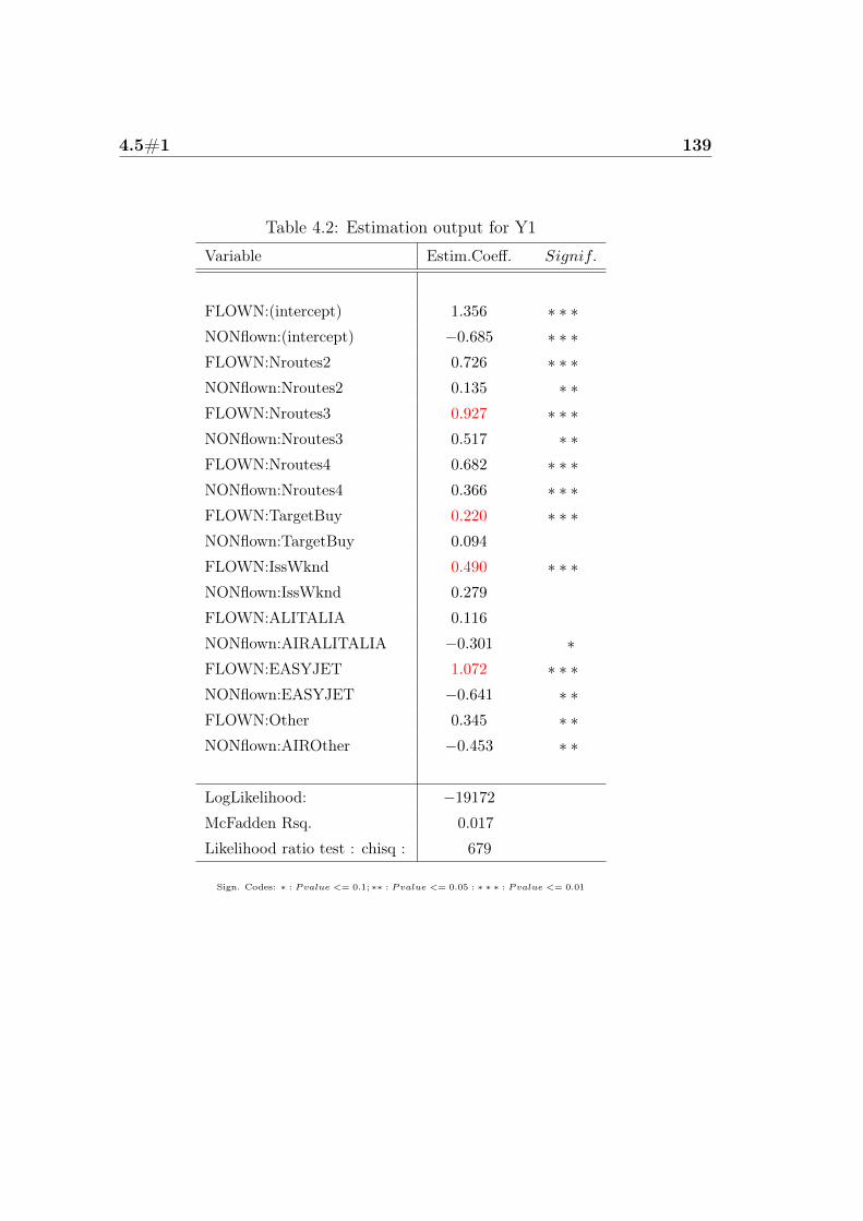
4.5#1 139
Table 4.2: Estimation output for Y1
Variable Estim.Coeff. Signif.
FLOWN:(intercept) 1.356 ∗ ∗ ∗NONflown:(intercept) −0.685 ∗ ∗ ∗FLOWN:Nroutes2 0.726 ∗ ∗ ∗NONflown:Nroutes2 0.135 ∗ ∗FLOWN:Nroutes3 0.927 ∗ ∗ ∗NONflown:Nroutes3 0.517 ∗ ∗FLOWN:Nroutes4 0.682 ∗ ∗ ∗NONflown:Nroutes4 0.366 ∗ ∗ ∗FLOWN:TargetBuy 0.220 ∗ ∗ ∗NONflown:TargetBuy 0.094
FLOWN:IssWknd 0.490 ∗ ∗ ∗NONflown:IssWknd 0.279
FLOWN:ALITALIA 0.116
NONflown:AIRALITALIA −0.301 ∗FLOWN:EASYJET 1.072 ∗ ∗ ∗NONflown:EASYJET −0.641 ∗ ∗FLOWN:Other 0.345 ∗ ∗NONflown:AIROther −0.453 ∗ ∗
LogLikelihood: −19172
McFadden Rsq. 0.017
Likelihood ratio test : chisq : 679
Sign. Codes: ∗ : Pvalue <= 0.1; ∗∗ : Pvalue <= 0.05 : ∗ ∗ ∗ : Pvalue <= 0.01
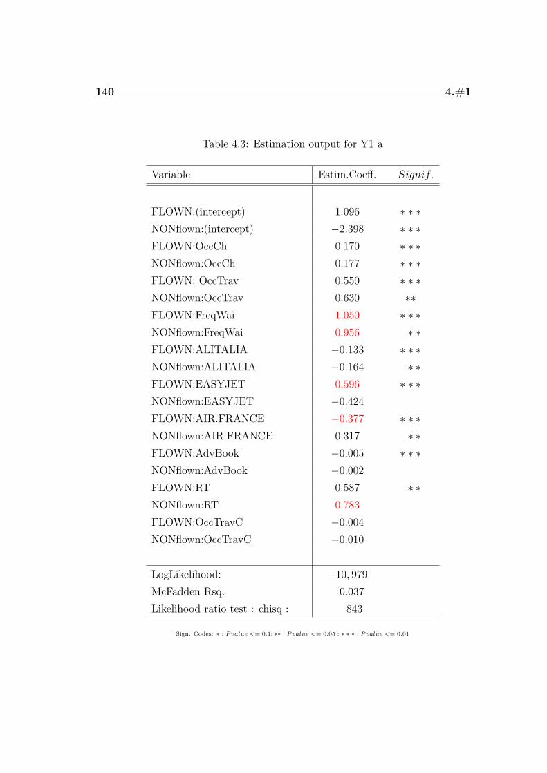
140 4.#1
Table 4.3: Estimation output for Y1 a
Variable Estim.Coeff. Signif.
FLOWN:(intercept) 1.096 ∗ ∗ ∗NONflown:(intercept) −2.398 ∗ ∗ ∗FLOWN:OccCh 0.170 ∗ ∗ ∗NONflown:OccCh 0.177 ∗ ∗ ∗FLOWN: OccTrav 0.550 ∗ ∗ ∗NONflown:OccTrav 0.630 ∗∗FLOWN:FreqWai 1.050 ∗ ∗ ∗NONflown:FreqWai 0.956 ∗ ∗FLOWN:ALITALIA −0.133 ∗ ∗ ∗NONflown:ALITALIA −0.164 ∗ ∗FLOWN:EASYJET 0.596 ∗ ∗ ∗NONflown:EASYJET −0.424
FLOWN:AIR.FRANCE −0.377 ∗ ∗ ∗NONflown:AIR.FRANCE 0.317 ∗ ∗FLOWN:AdvBook −0.005 ∗ ∗ ∗NONflown:AdvBook −0.002
FLOWN:RT 0.587 ∗ ∗NONflown:RT 0.783
FLOWN:OccTravC −0.004
NONflown:OccTravC −0.010
LogLikelihood: −10, 979
McFadden Rsq. 0.037
Likelihood ratio test : chisq : 843
Sign. Codes: ∗ : Pvalue <= 0.1; ∗∗ : Pvalue <= 0.05 : ∗ ∗ ∗ : Pvalue <= 0.01
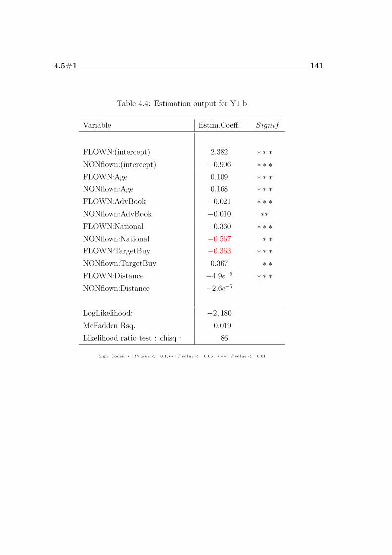
4.5#1 141
Table 4.4: Estimation output for Y1 b
Variable Estim.Coeff. Signif.
FLOWN:(intercept) 2.382 ∗ ∗ ∗NONflown:(intercept) −0.906 ∗ ∗ ∗FLOWN:Age 0.109 ∗ ∗ ∗NONflown:Age 0.168 ∗ ∗ ∗FLOWN:AdvBook −0.021 ∗ ∗ ∗NONflown:AdvBook −0.010 ∗∗FLOWN:National −0.360 ∗ ∗ ∗NONflown:National −0.567 ∗ ∗FLOWN:TargetBuy −0.363 ∗ ∗ ∗NONflown:TargetBuy 0.367 ∗ ∗FLOWN:Distance −4.9e−5 ∗ ∗ ∗NONflown:Distance −2.6e−5
LogLikelihood: −2, 180
McFadden Rsq. 0.019
Likelihood ratio test : chisq : 86
Sign. Codes: ∗ : Pvalue <= 0.1; ∗∗ : Pvalue <= 0.05 : ∗ ∗ ∗ : Pvalue <= 0.01
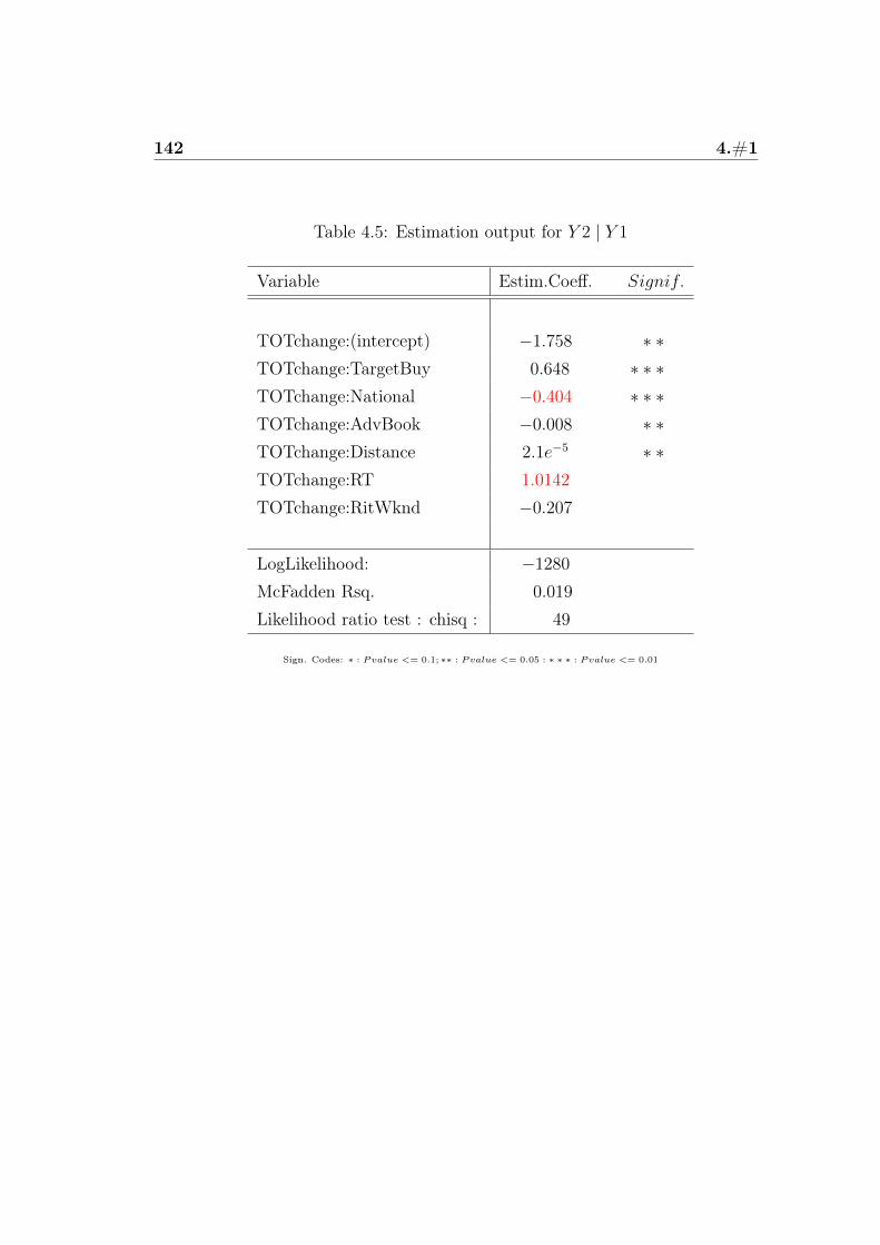
142 4.#1
Table 4.5: Estimation output for Y 2 | Y 1
Variable Estim.Coeff. Signif.
TOTchange:(intercept) −1.758 ∗ ∗TOTchange:TargetBuy 0.648 ∗ ∗ ∗TOTchange:National −0.404 ∗ ∗ ∗TOTchange:AdvBook −0.008 ∗ ∗TOTchange:Distance 2.1e−5 ∗ ∗TOTchange:RT 1.0142
TOTchange:RitWknd −0.207
LogLikelihood: −1280
McFadden Rsq. 0.019
Likelihood ratio test : chisq : 49
Sign. Codes: ∗ : Pvalue <= 0.1; ∗∗ : Pvalue <= 0.05 : ∗ ∗ ∗ : Pvalue <= 0.01
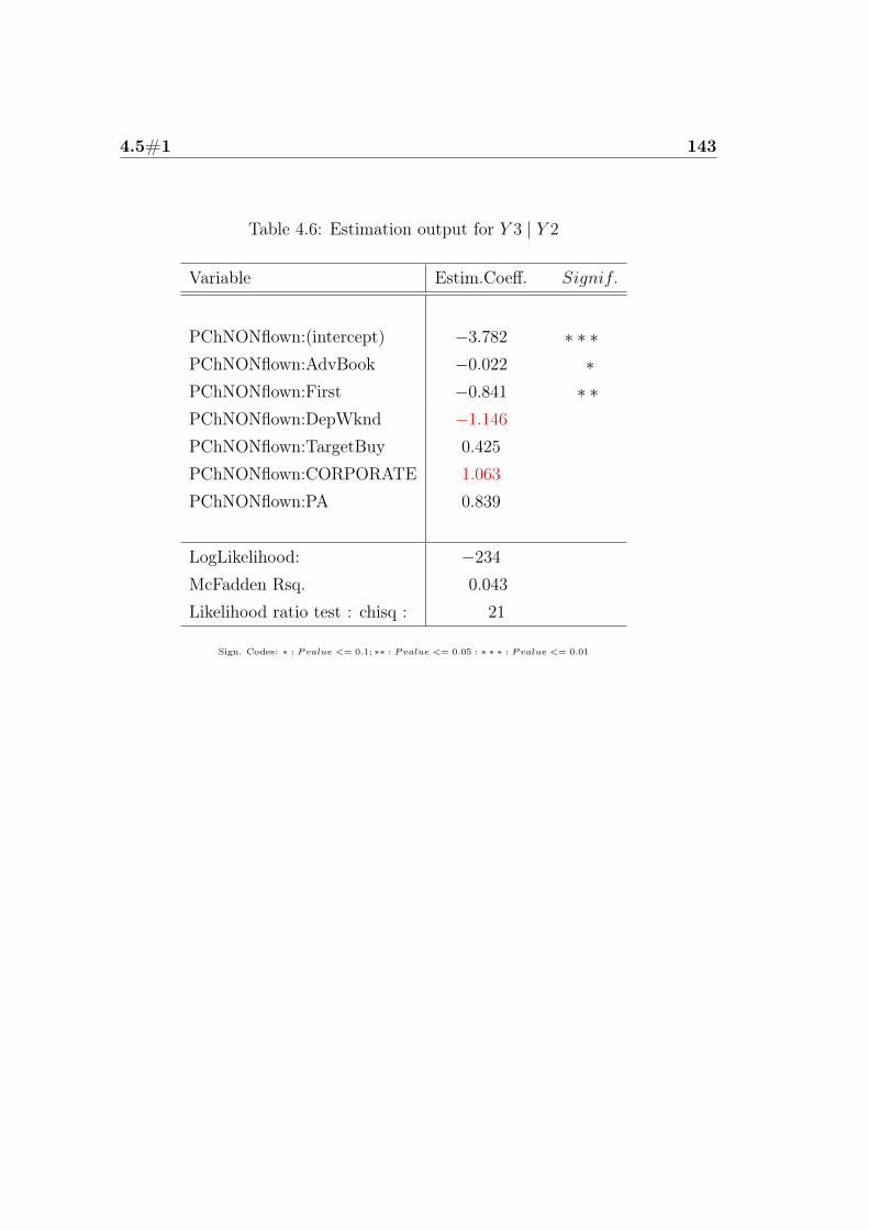
4.5#1 143
Table 4.6: Estimation output for Y 3 | Y 2
Variable Estim.Coeff. Signif.
PChNONflown:(intercept) −3.782 ∗ ∗ ∗PChNONflown:AdvBook −0.022 ∗PChNONflown:First −0.841 ∗ ∗PChNONflown:DepWknd −1.146
PChNONflown:TargetBuy 0.425
PChNONflown:CORPORATE 1.063
PChNONflown:PA 0.839
LogLikelihood: −234
McFadden Rsq. 0.043Likelihood ratio test : chisq : 21
Sign. Codes: ∗ : Pvalue <= 0.1; ∗∗ : Pvalue <= 0.05 : ∗ ∗ ∗ : Pvalue <= 0.01
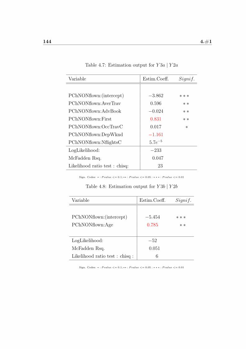
144 4.#1
Table 4.7: Estimation output for Y 3a | Y 2a
Variable Estim.Coeff. Signif.
PChNONflown:(intercept) −3.862 ∗ ∗ ∗PChNONflown:AverTrav 0.596 ∗ ∗PChNONflown:AdvBook −0.024 ∗ ∗PChNONflown:First 0.831 ∗ ∗PChNONflown:OccTravC 0.017 ∗PChNONflown:DepWknd −1.161
PChNONflown:NflightsC 5.7e−5
LogLikelihood: −233
McFadden Rsq. 0.047
Likelihood ratio test : chisq: 23
Sign. Codes: ∗ : Pvalue <= 0.1; ∗∗ : Pvalue <= 0.05 : ∗ ∗ ∗ : Pvalue <= 0.01
Table 4.8: Estimation output for Y 3b | Y 2b
Variable Estim.Coeff. Signif.
PChNONflown:(intercept) −5.454 ∗ ∗ ∗PChNONflown:Age 0.785 ∗ ∗
LogLikelihood: −52
McFadden Rsq. 0.051
Likelihood ratio test : chisq : 6
Sign. Codes: ∗ : Pvalue <= 0.1; ∗∗ : Pvalue <= 0.05 : ∗ ∗ ∗ : Pvalue <= 0.01
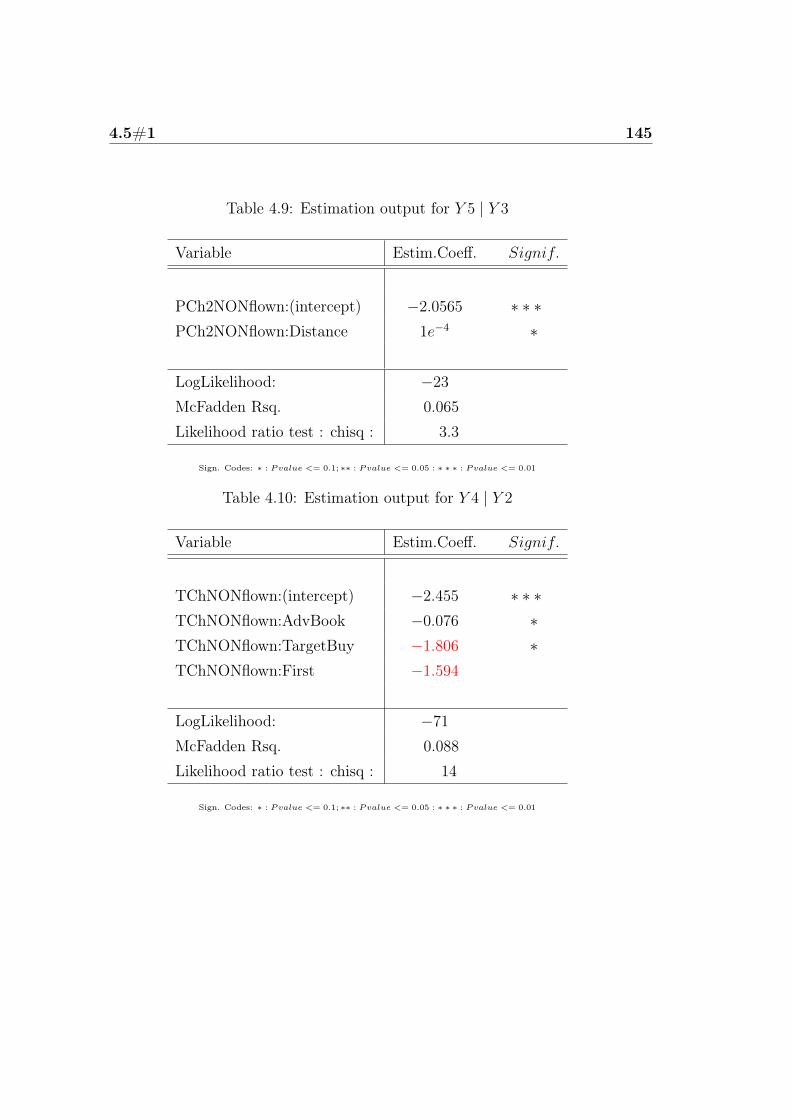
4.5#1 145
Table 4.9: Estimation output for Y 5 | Y 3
Variable Estim.Coeff. Signif.
PCh2NONflown:(intercept) −2.0565 ∗ ∗ ∗PCh2NONflown:Distance 1e−4 ∗
LogLikelihood: −23
McFadden Rsq. 0.065
Likelihood ratio test : chisq : 3.3
Sign. Codes: ∗ : Pvalue <= 0.1; ∗∗ : Pvalue <= 0.05 : ∗ ∗ ∗ : Pvalue <= 0.01
Table 4.10: Estimation output for Y 4 | Y 2
Variable Estim.Coeff. Signif.
TChNONflown:(intercept) −2.455 ∗ ∗ ∗TChNONflown:AdvBook −0.076 ∗TChNONflown:TargetBuy −1.806 ∗TChNONflown:First −1.594
LogLikelihood: −71
McFadden Rsq. 0.088Likelihood ratio test : chisq : 14
Sign. Codes: ∗ : Pvalue <= 0.1; ∗∗ : Pvalue <= 0.05 : ∗ ∗ ∗ : Pvalue <= 0.01
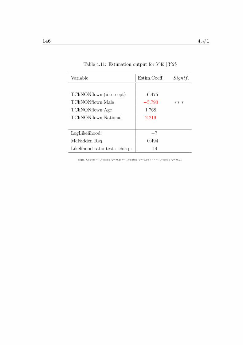
146 4.#1
Table 4.11: Estimation output for Y 4b | Y 2b
Variable Estim.Coeff. Signif.
TChNONflown:(intercept) −6.475
TChNONflown:Male −5.790 ∗ ∗ ∗TChNONflown:Age 1.768
TChNONflown:National 2.219
LogLikelihood: −7
McFadden Rsq. 0.494Likelihood ratio test : chisq : 14
Sign. Codes: ∗ : Pvalue <= 0.1; ∗∗ : Pvalue <= 0.05 : ∗ ∗ ∗ : Pvalue <= 0.01
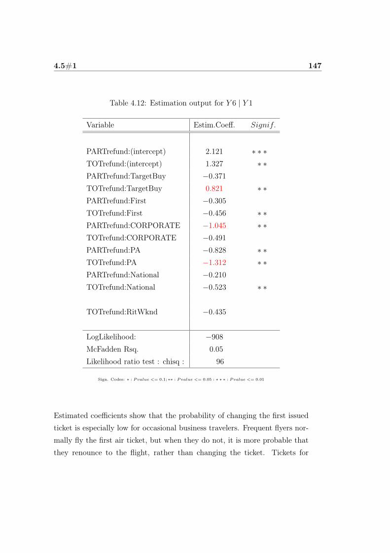
4.5#1 147
Table 4.12: Estimation output for Y 6 | Y 1
Variable Estim.Coeff. Signif.
PARTrefund:(intercept) 2.121 ∗ ∗ ∗TOTrefund:(intercept) 1.327 ∗ ∗PARTrefund:TargetBuy −0.371
TOTrefund:TargetBuy 0.821 ∗ ∗PARTrefund:First −0.305
TOTrefund:First −0.456 ∗ ∗PARTrefund:CORPORATE −1.045 ∗ ∗TOTrefund:CORPORATE −0.491
PARTrefund:PA −0.828 ∗ ∗TOTrefund:PA −1.312 ∗ ∗PARTrefund:National −0.210
TOTrefund:National −0.523 ∗ ∗
TOTrefund:RitWknd −0.435
LogLikelihood: −908
McFadden Rsq. 0.05
Likelihood ratio test : chisq : 96
Sign. Codes: ∗ : Pvalue <= 0.1; ∗∗ : Pvalue <= 0.05 : ∗ ∗ ∗ : Pvalue <= 0.01
Estimated coefficients show that the probability of changing the first issuedticket is especially low for occasional business travelers. Frequent flyers nor-mally fly the first air ticket, but when they do not, it is more probable thatthey renounce to the flight, rather than changing the ticket. Tickets for
148 4.#1
flights operated by Alitalia are more likely changed, those issued by Easyjetare more probably flown, while flights operated by Air France are more oftensubject to renounce.
As it may be expected, the longer the advance booking time, thehigher the probability of change. Moreover, it is more likely that a busi-ness traveler renounces to a round trip (than a one way journey) but it isless probable that he changes the ticket. Travelers working for companiesoccasionally requiring them to fly tend to change ticket more often. Whilethe probability of changing ticket decreases as the flyer’s age increases, theprobability of renounce becomes higher for older workers. It is more likelythat a national flight is changed, but the effect of the distance covered bythe journey is very small. Single-route tickets are changed more often, multi-route first issued ones are more likely flown.
If the ticket is booked during the weekend, then it is highly probablethat it will be flown, it will be hardly changed, maybe because journeys or-ganized outside of work are motivated by emergencies. Once totally changedthe first purchased ticket, it is much more likely that it will be changedagain, or that the worker will renounce to the flight, if the business traveleris a female, maybe because women are often in charge of caregiving, for bothchildren and the oldest members of the family. The particular contract of-fered by Seneca, Target-buy, appears to make travelers incline to renounce,rather than to change flight.
As already warned, these results are not very reliable. Typically, Dis-crete Choice Models work better with information about the decision-makerand alternative-specific variables, but in this case they are not available (insufficient quantity and quality). As a consequence, the TMC is recommendedto collect, in the future, more data about the characteristics of the businesstravelers, as the problems in the present empirical analysis and the qualita-tive study of the business issue suggest that they should be an importantpredictor for the behavior of business travelers.

4.5#1 149
However, a general finding important from the phenomenic perspec-tive, is that there are some characteristics, of the flight, the ticket, the com-pany and the traveler, that can help predicting the behavior of the businessflyer. If TMCs or corporate travel departments extensively collect and takethem into account, they should be able to choose the optimal fare for eachtraveler, for each flight.

150 4.#1
Chapter 5
Predicting air tickts’ outcomes
5.1 Prediction problems
The models, the estimation outputs of which are reported above, describethe estimation sample ’to the best’, given the available information. To findthe best predictor, all of the models (m = 1, . . . ,M) obtained at each stepof the first two Stepwise procedures are subjected to external validationon the forecasting sample. According to the ML principle, the outcome,predicted by the m-th model, for the i-th flight, is that (j∗) for whichthe estimated conditional probability is the highest of the row vector Pi,m[yi]:
yi,m = j∗ ⇔ Pi,m[yi = j∗] = MAXPi,m[yi = j];∀j ∈ Ry
(5.1)
But the discriminatory power of the available independent variables is excep-tionally low, as expected looking at the values of McFadden R-square. Thus,the estimated conditional probabilities are either very close to the samplemarginal frequencies or largely biased. In fact, right from the first node (Y 1):
151
152 5.#1
• the Exact Classification Rate (ECR) of models ("a") includingvariables describing the past behavior of travelers is less than 33%, soless than that of a completely random classification;
• for the other models ECR = 91% but they always classify any ticketas flown.
Therefore, these models are useless in prediction and do not allow to classifyoutcomes following the first one.
The causes of such a low discriminatory power, are essentially three:
• In order to predict the travelers’ decisions correctly, through DiscreteChoice Models, information about the decision-makers and alternative-specific variables would be needed, while sufficient information, in termsof both quantity and quality, is available only about flights and tickets’characteristics (nonetheless, the MLM is the only viable specification,as there is no enough information to estimate more complex models).
• A few client companies purchase most of the flights (80/20 rule of sales),that are nearly identical (they always depart from the airport closestto the company, are operated by the same airline because travelerswant to accumulate miles on their frequent flyer programs, are alwaysof the same class and so forth), so that they show the same values ofexplanatory variables and, among numerous tickes, just very few arenot flown.
• The phenomenon could be in influenced by some factors not observedor appreciable in the estimation sample, but present in the forecastingsample.

5.2#1 153
As there is no possibility to collect further information and the composition ofSeneca’s client portfolio is given, an attempt is made to act on the last causeof prediction problems. So what element could influence the phenomenon,but is not observed in the estimation sample?
• As mentioned in the literature review, some extant studies about busi-ness travel suggest that it may be a sort of seasonal pattern, related tovacation periods.
• The qualitative study of the phenomenon highlights that changes andwaivers, in business travel, are often determined by personal and rela-tional reasons, especially by the desire to spend the festivities with thefamily.
If the estimation sample covered a whole year, this would prompt to inserta dummy indicator of vacation periods D and estimate its effect δ. But,since the observations used for estimation span only seven months, it is justpossible to guess a ’vacation effect’.
5.2 Guess-based predictions
Guesses have been used in Statistics since its birth, in the form of subjectiveprediction (eg. in Delphy method) or, slightly more recently, as priorinformation, in the Bayesian approach. In the present case, none of the twoortodox solutions is viable. In fact, the literature about business travel andthe qualitative study of the context provide a too vague suggestion, notdirectly expressible in the out-of-sample classification, nor elicitable in aprior distribution of the coefficients of the models.
Thus, an alternative and very simple method is adopted: the guesson the ’vacation effect’, δ, is added directly in the estimated models for Y 1.In practice, a dummy variable D is constructed as the interaction: D1 ∗D2,where each element of D1, d1i = 1 if the i-th flight is booked in December
154 5.#1
or August, zero otherwise; each element of D2, d2i = 1 if the departure dateof the i-th fligh is in December or August, zero otherwise.Then, guessing that during vacations the probability that a ticket is notflown should be higher than the probability that it is flown, in considerationof the fact that renounce (Nf) is the most difficult outcome to be forecasted(and the most rarely observed), δ is chosen such that:
δNO = αNO + βNO − q0,NO (5.2)
δFl = −(αFl + βFl) + q0,F l (5.3)
with q0 real number, small enough such that:
∃i : ifPi[y1i = Nf ] = MAXP [y1 = Nf ]
∧Di = 1 (5.4)
⇒ Pi[y1i = Nf ] = MAXPi[y1]
(5.5)
⇒ yi = Nf (5.6)
but big enough so that the model does not collapse on the intercept andvacation effect only:
logit(Y 1) = α + δD + e (5.7)
By adding δD, all of the models’ predicting capability improves, from acorporate perspective: although the ECR decreases, now it is possible tocorrectly classify some tickets as changed and non-flown, the two most eco-nomically relevant outcomes (the correct prediction of which generates thehighest saving). So the best predictor is selected, as the one yielding:
• Max ECR;
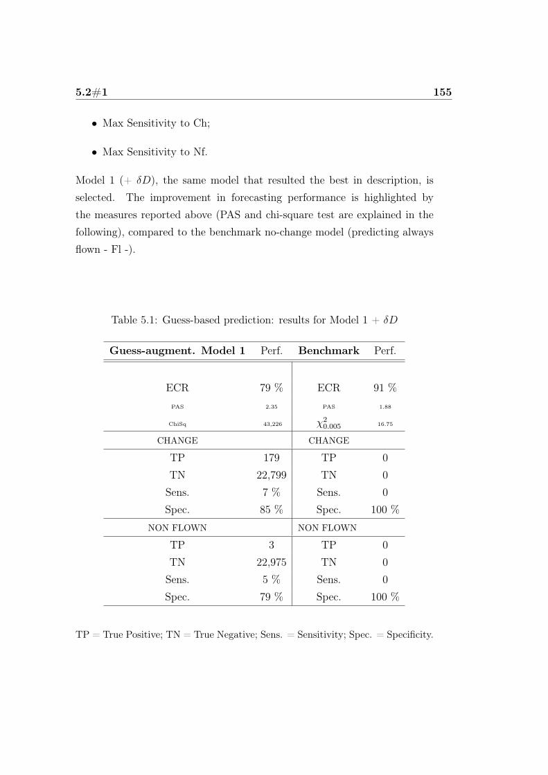
5.2#1 155
• Max Sensitivity to Ch;
• Max Sensitivity to Nf.
Model 1 (+ δD), the same model that resulted the best in description, isselected. The improvement in forecasting performance is highlighted bythe measures reported above (PAS and chi-square test are explained in thefollowing), compared to the benchmark no-change model (predicting alwaysflown - Fl -).
Table 5.1: Guess-based prediction: results for Model 1 + δD
Guess-augment. Model 1 Perf. Benchmark Perf.
ECR 79 % ECR 91 %PAS 2.35 PAS 1.88
ChiSq 43,226 χ20.005 16.75
CHANGE CHANGE
TP 179 TP 0TN 22,799 TN 0Sens. 7 % Sens. 0Spec. 85 % Spec. 100 %
NON FLOWN NON FLOWN
TP 3 TP 0TN 22,975 TN 0Sens. 5 % Sens. 0Spec. 79 % Spec. 100 %
TP = True Positive; TN = True Negative; Sens. = Sensitivity; Spec. = Specificity.

156 5.#1
The comparison shows that, adding the guess on the vacation effect to Model1, its overall forecasting performance does improve, in economic terms.
But what would be the value of δ if it was possible to estimate it ondata actually affected by this vacation effect? In order to approximate it:
• 500 replicas of the independent variables are drawn from the wholedatabase (estimation sample + forecasting sample, for getting a wholeyear), through a non−parametric, non−stratified bootstrap withreplacement (Xboot);
• For each replica, the dependent variable Y 1 is generated from theguess-augmented model (1):
˜logit(Y 1) = α1+βNT1NumTratteboot+βEW1EmissWkndboot+βair1Airlineboot+βTB1TargetBuyboot+δDboot+e1
(5.8)
where e1 ∼ Gumbel(0, 1).
• D is added to specification 1 and all the coefficients (including δ) areestimated ML on each bootstrap sample.
• All the coefficients are significant at the chosen 0.3 P−value threshold,except for δ, which is significant only in the 10% of cases.
• Each coefficient is averaged over the 500 samples (α and δ included),
βh,boot =
500∑r=1
βh,r
500.
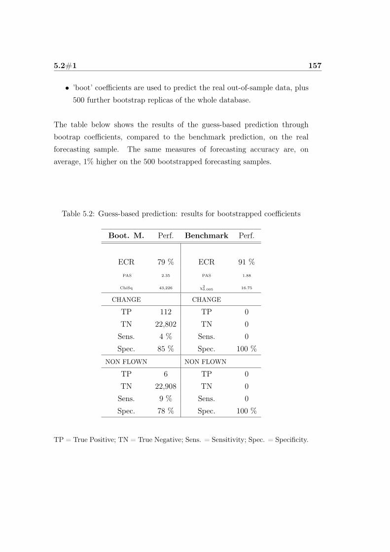
5.2#1 157
• ’boot’ coefficients are used to predict the real out-of-sample data, plus500 further bootstrap replicas of the whole database.
The table below shows the results of the guess-based prediction throughbootrap coefficients, compared to the benchmark prediction, on the realforecasting sample. The same measures of forecasting accuracy are, onaverage, 1% higher on the 500 bootstrapped forecasting samples.
Table 5.2: Guess-based prediction: results for bootstrapped coefficients
Boot. M. Perf. Benchmark Perf.
ECR 79 % ECR 91 %PAS 2.35 PAS 1.88
ChiSq 43,226 χ20.005 16.75
CHANGE CHANGE
TP 112 TP 0TN 22,802 TN 0Sens. 4 % Sens. 0Spec. 85 % Spec. 100 %
NON FLOWN NON FLOWN
TP 6 TP 0TN 22,908 TN 0Sens. 9 % Sens. 0Spec. 78 % Spec. 100 %
TP = True Positive; TN = True Negative; Sens. = Sensitivity; Spec. = Specificity.
158 5.#1
It is possible to see a slight increase in the forecasting performance of themodel, thanks to the bootstrap. But the most interesting result is that, com-paring predictions made through the selected model, as re-estimated with thevacation effect, with those obtained using the coefficients estimated withoutthe vacation-effect, on the 500 bootstrap forecasting samples (including ob-servations for the whole year), the forecasting performance improves also onthe first half of the samples (corresponding to the estimation sample, but inits bootstrap replica). In fact, on average, 2 tickets are classified as renounces(Nf), and 4 as changes (Ch), while none was classified differently than flown(Fl) through the model estimated without δD.
But is this improvement enough to help the TMC choosing the optimalfare, in order to minimize the cost of flights?
5.3 Economic evaluation of the forecasting perfor-
mances
Since the prediction of air tickets’ outcomes is aimed at deciding which fareto buy (F∗), in order to minimize the cost of flights, the problem addressedin the present work is economic in nature. Therefore, the wanted predictor isnot the one yielding the highest values of statistical measures of forecastingcapability, but that producing the biggest saving. As a consequence, theforecasting performance of estimated models should be assessed non justthrough statistical measures, but also and more relevantly through theeconomic result, obtainable thanks to the predictors.
In general, the economic performance of a predictor should beevaluated based on
Ci − CT∗,i(E[Yi]) (5.9)
But:
5.3#1 159
• for choosing F∗i it would be necessary to know the price of everypossible Ti;
• to simulate the price of the 3 X N Ti, a reference price, with constantaverage difference from the price of all T,∀i (for flights with differentcharacteristics), is required;
• as reference price, those of the full fare and the IATA fare (referencefare, as calculated by the International Air Transport Association) areavailable, but none of them has that property;
• the type of fare is recorded only in 108 cases over 29,252, in theforecasting sample;
• moreover, in the forecasting sample, in 19,974 cases over 29,252 Ci isnot computable, as the price of each ticket and the cost of each change,is missing.
As a consequence, a simplification and an approximation are required,for developing a cost function useful to the aim of assessing predictors’performances and also business-specific.
First, the price of each ticket Pri is approximated with the averagecost per Km of the corresponding fare, times the kilometers covered by thei-th flight (P ri).Afterward, the following hypotheses are made:
1. The possible fares are only two: fixed and flexible. This assumption isdefinitely meaningful, as, if the business traveler flies the first issued
160 5.#1
ticket, than the optimal fare is the cheapest one and there is nocheaper fare than the fixed one. If the ticket is changed, the optimalfare is the one charging the lowest penalty and the flexible fare allowsas many changes as the flyer wants, all for free. But also if the travelerrenounces to the flight the flexible fare is oprimal, as it is the only fullrefundable one.
2. In the absence of a reliable predictor, the benchmark purchasingstrategy consists in buying always the fixed fare. It is based on theconsideration that 85% of the first issued tickets are flown, in theestimation sample, but it is also the strategy commonly prescribedby corporate travel departments, in the corporate travel policy of bigcorporations.
3. If the traveler changes the ticket, the change is made close to thedeparture date, when discounted fares tend to be no more available.Moreover, the flyer is assumed to guess that maybe he will have tochange more than once, or, finally, could even renounce to the flight,so that he will find more convenient to get a flexible fare.
4. As a consequence, once purchased a fixed fare, in case of change, aflexible ticket is chosen.
5. Prices increase as the date of departure approaches. This is often truein reality, even if the price depends on the plane filling rate. However,this means that a flexible fare, purchased at the time of the firstissuance, has a lower price than a flexible fare bought closer to thedeparture dare.

5.3#1 161
Accordingly, the cost functions, for the benchmark strategy and for predic-tors (M) respectively, are:
Table 5.3: Cost function
Obs. Benchmark EM [yi] = Ch EM [yi] = Nf EM [yi] = Fl
Ch Prfix + Prflex,t+k Prflex,t Prflex,t Prfix + Prflex,t+k
Nf Prfix 0 0 Prfix
Fl Prfix Prflex,t Prflex,t Prfix
where t is the date of issuance and t+ k is the date of change.Then, the loss function for predictors is given by the difference
between their cost function and that of the benchmark:
Table 5.4: Loss function
Obs. EM [yi] = Ch EM [yi] = Nf EM [yi] = Fl
Ch Prfix + Prflex,t+k − Prflex,t Prfix + Prflex,t+k − Prflex,t 0Nf Prfix Prfix 0Fl −[Prflex,t − Prfix] −[Prflex,t − Prfix] 0
Thus, if the m−th model predicts that the first issued ticket will be flown,a fixed fare is bought and in case it is changed, the cost of the flight is

162 5.#1
given by the sum of the price of the fixed fare and the price of the flexiblefare, bought closer to the departure date; in both cases that the travelerrenounces to the flight and that he flies the first ticket, the cost equals theprice of the fixed fare. In this case the cost function for the benchmark isidentical to that of the predictor, so that the loss function in zero each timesthe model predicts Fl.
Whether the model predicts that the first issued ticket will bechanged, whether it forecasts that the traveler will renounce to the flight, afixed fare is purchased. Thus, the cost of the flight is always equal to theprice of the flexible fare bought at the time of the first issuance t, exceptin case the traveler renounces to the flight. In that case, the price of theticket is completely refundend, so that the non-flown flight costs nothing.Therefore, if the predictor forecasts change or renounce and the travelerchanges the ticket, the gain (saving) equals the fixed price plus the (moreexpensive) flexible price (for the change), minus the lower price of theflexible fare bought time before. In case the traveler renounces to the flight,then the gain is equal to the fixed price.
Only whether the first issued ticket is flown and the model forecastsone of the other two outcomes, it yields a loss, equal to the difference inprice between a fixed and a flexible fare (in red in the above table).
The value of such loss function for the guess−based predictor is −1, 372, 852,thus the benchmark strategy greatly outperforms it. Clearly, the mis-classification rate for flown tickets is very high, because, in order to correctlyclassify at least a few tickets as changed and renounced, the vacation effectis so heavy, that leads to classify as non-flown also a lot of actually flowntickets. This evidence points out that, even if there seems to be a vacationeffect, increasing the probability that a ticket is changed or non flown, theprobability that it is flown is still higher, also for flights booked in August or

5.4#1 163
December and departing in the same months.Therefore, another alternative solution, to try to increase the predic-
tion capability of models estimated with the poor available information, mustbe searched.
5.4 A new classification algorithm
For trying to improve the economic performance of predictors, it seemsappropriate to replace the ML principle with the economic one, because theaim of the present work is minimizing the cost of flights.
According to the economic principle, the classification rule should be:
ifPi[yi = yj] > h∗ ⇒ Eh∗[yi] = yj (5.10)
where
h∗ :∑i
Ey,h∗[CF∗i,i]− Ci = MIN
∑i
Eyh[CF∗i,i]− Ci;h ∈ [0, 1]
(5.11)
But, as mentioned above, to claculate the cost of a flight corresponding toits fare CF,i, the price of each ticket Pri and its fare typology Fi should beknown. The cost function described in the previous section can be employedto approximate the expected value of the flight, for the fare that the modelsuggests to be optimal Eyh[CF∗,i]. But the lack of data about the actualcost of the flight cannot be meaningfully replaced with any approximation,in the present context, because here the aim is to compare the amount spentbuying a fare chosen with no predictor with the figure that would have beenspent if the proposed models were used. Therefore a further simplification is
164 5.#1
necessary.Analyzing to the loss function illustrated above, it is found that:
• The only cases in which a predictor yields a loss, if compared to thebenchmark strategy, is when it forecasts that the ticket’s outcome willbe change or renounce, but the traveler actually flies the first issuedticket.
• Each time a predictor forecasts that the flyer will change or waiverthe ticket and one of these two behaviors happens, compared to thebenchmark strategy, it produces a gain that is higher than the possibleloss:
Prfix + Prflex,t+k − Prflex,t > Prfix > Prflex,t − Prfix (5.12)
• Nonetheless, it is very difficult to beat the benchmark strategy, becausea lot of tickets are classified as not flown, if the hand is forced enoughtto correctly predict a few changes and renounces.
As a consequence, the aim of a new classification rule should be to obtainthe highest possible sensitivity to changes and renounces, while keeping thenumber of incorrectly classified actually flown tickets as low as possible.Therefore, the threshold h∗ is chosen maximizing the sensitivity to Ch andNf (outcomes generating relative gains), once controlled for the misclassifi-cation rate of Fl:
ifPi[yi = yj] > h∗ ⇒ Eh∗[yi] = yj (5.13)
where h*:
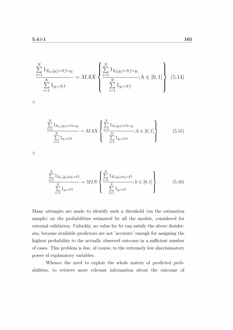
5.4#1 165
N∑i=1
1Eh∗[yi]=Nf=yi
N∑i=1
1yi=Nf
= MAX
N∑i=1
1Eh[yi]=Nf=yi
N∑i=1
1yi=Nf
;h ∈ [0, 1]
(5.14)
∧
N∑i=1
1Eh∗[yi]=Ch=yi
N∑i=1
1yi=Ch
= MAX
N∑i=1
1Eh[yi]=Ch=yi
N∑i=1
1yi=Ch
;h ∈ [0, 1]
(5.15)
∧
N∑i=1
1Eh∗[yi] 6=yi=Fl
N∑i=1
1yi=Fl
= MIN
N∑i=1
1Eh[yi]6=yi=Fl
N∑i=1
1yi=Fl
;h ∈ [0, 1]
(5.16)
Many attempts are made to identify such a threshold (on the estimationsample) on the probabilities estimated by all the models, considered forexternal validation. Unluckly, no value for h∗ can satisfy the above desider-ata, because available predictors are not ’accurate’ enough for assigning thehighest probability to the actually observed outcome in a sufficient numberof cases. This problem is due, of course, to the extremely low discriminatorypower of explanatory variables.
Whence the need to exploit the whole matrix of predicted prob-abilities, to retrieve more relevant information about the outcome of
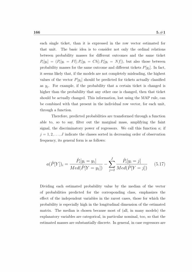
166 5.#1
each single ticket, than it is expressed in the row vector estimated forthat unit. The basic idea is to consider not only the ordinal relationsbetween probability masses for different outcomes and the same ticketPi[yi] = (Pi[yi = Fl];Pi[yi = Ch];Pi[yi = Nf ]), but also those betweenprobability masses for the same outcome and different tickets P [yj]. In fact,it seems likely that, if the models are not completely misleading, the highestvalues of the vector P [yj] should be predicted for tickets actually classifiedas yj. For example, if the probability that a certain ticket is changed ishigher than the probability that any other one is changed, then that ticketshould be actually changed. This information, lost using the MAP rule, canbe combined with that present in the individual row vector, for each unit,through a function.
Therefore, predicted probabilities are transformed through a functionable to, so to say, filter out the marginal mass, amplifying the faintsignal, the discriminatory power of regressors. We call this function a; ifj = 1, 2, . . . , J indicate the classes sorted in decreasing order of observationfrequency, its general form is as follows:
a(P [Y ])i =Pi[yi = y1]
Med(P [Y = y1])−
J∑j=2
Pi[yi = j]
Med(P [Y = j])(5.17)
Dividing each estimated probability value by the median of the vectorof probabilities predicted for the corresponding class, emphasizes theeffect of the independent variables in the rarest cases, those for which theprobability is especially high in the longitudinal dimension of the estimatedmatrix. The median is chosen because most of (all, in many models) theexplanatory variables are categorical, in particular nominal, too, so that theestimated masses are substantially discrete. In general, in case regressors are

5.4#1 167
continuous variables, it is likely that replacing the median with the mean, inthe above function, will yield better results.
Subtracting the summation of the masses predicted for the lessfrequently observed outcomes (observed in the estimation sample), dividedby the respective medians, from the same transformation of the probabilityestimated for the most frequently observed class, allows to identify thoseindividuals (tickets) for which it is nearly sure that they will be actuallyclassifyed as y1. The functional form of a is such that it is expected to workespecially well in cases, like the present one, where y1 is observed definitelymuch more often than the other outcomes (85% of the times). However, itis exactly in this kind of situations that such a function is more needed inbusiness environment where the database is affected by the 80/20 rule ofsale or similar specificities of the corporate activities.
Then, 2 thresholds h∗1 and h∗unc are identified on the vectora = [a1, . . . , ai, . . . , aN ], on the estimation sample, instead than j − 1
thresholds on the raw vectors of estimated probabilities. In general:
If ai(P [Y ]) ≥ h∗1 ⇒ Eh∗[yi] = y1 (5.18)
where:
h∗1 :
∑i
1Eh∗1 [yi]=yi∑i
1ai(P [Y ])≥h∗1= MAX
∑i
1Eh[yi]=yi∑i
1ai(P [Y ])≥h1
(5.19)
if h∗unc < ai(P [Y ]) < h∗1 ⇒ Eh∗[yi] =?⇒ Eh∗[yi] = y1 (5.20)
Then:

168 5.#1
if ai(P [Y ]) ≤ h∗unc∧Pi[yi = y2]
Med(P [y = y2])= MAX
P [y = j]
Med(P [Y = j]); j = 2, . . . , J
⇒ Eh∗[yi] = y2
(5.21)
if ai(P [Y ]) ≤ h∗unc∧Pi[yi = y3]
Med(P [y = y3])= MAX
P [y = j]
Med(P [Y = j]); j = 2, . . . , J
⇒ Eh∗[yi] = y3
(5.22)
. . . otherwise Eh∗[yi] = yJ
The first threshold h∗1 leaves the individuals that will be ’nearly surely’observed as belonging to the first class (in decreasing order of observationfrequency) above its value. Its value is chosen maximizing the sensitivity tothis class, considering only individuals whose value of ai is above h∗1. Italso constitutes the upper limit of an ’uncertainty interval’, defined by h∗uncas its lower bound.
Units for which ai belongs to this uncertainty interval, are charac-terized by a lack of information sufficient to correctly classify them, evenin a small percentage of cases. The discriminatory power of independentvariables is essentially null in these cases, so that the uncertainty abouttheir outcome is as wide as if no regressor were available. Therefore, theestimation sample marginal masses are considered, so that the predicion,for these individuals, coincides with the most frequently observed outcome.This choice is especially appropriate in the present case, because whenevera ticket is forecasted as flown, the purchase of a fixed fare is suggested. Andthe fixed fare is the one always chosen through the benchmark strategy,so that the relative loss, for the model, is null, as well as the relative gain(saving).

5.4#1 169
Units for which the value of ai is lower than h∗unc display Pi[yi=yj 6=1]
Med(P [y=yj 6=1])
large enough to be classified with an acceptable degree of reliability. Thus,the values of the transformations for the remaining J − 1 classes arecompared and the highest one identifies the predicted outcome.
In the present case, the algorithm is specifically as follows:
ai(P [Y ]) =Pi[yi = Fl]
Med(P [y = Fl])−
Pi[yi = Ch]
Med(P [y = Ch])+
Pi[yi = Nf ]
Med(P [Y = Nf ])
(5.23)
Then, the threshold h∗fl, for the most frequently observed class, is deter-mined on the estimation sample:
if ai(P [Y ]) ≥ h∗fl ⇒ Eh∗[yi] = Fl (5.24)
where
h∗Fl :
∑i
1Eh∗[yi]=yi=Fl∑i
1ai(P [Y ])≥h∗fl= MAX
∑i
1Eh[yi]=yi=Fl∑i
1ai(P [Y ])≥hfl
(5.25)
below which, the uncertainty interval is defined, with lower bond h∗unc:
if h∗unc < ai(P [Y ]) < h∗fl ⇒ Eh∗[yi] =? (5.26)
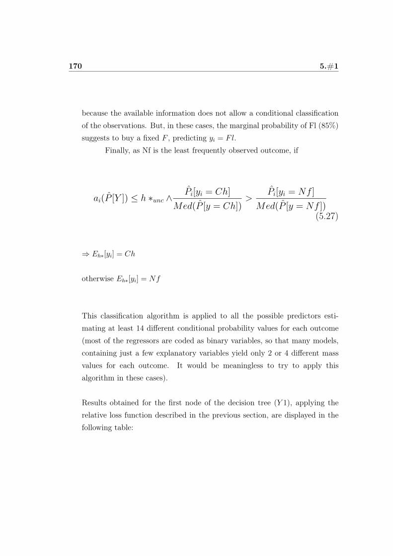
170 5.#1
because the available information does not allow a conditional classificationof the observations. But, in these cases, the marginal probability of Fl (85%)suggests to buy a fixed F , predicting yi = Fl.
Finally, as Nf is the least frequently observed outcome, if
ai(P [Y ]) ≤ h ∗unc ∧Pi[yi = Ch]
Med(P [y = Ch])>
Pi[yi = Nf ]
Med(P [y = Nf ])(5.27)
⇒ Eh∗[yi] = Ch
otherwise Eh∗[yi] = Nf
This classification algorithm is applied to all the possible predictors esti-mating at least 14 different conditional probability values for each outcome(most of the regressors are coded as binary variables, so that many models,containing just a few explanatory variables yield only 2 or 4 different massvalues for each outcome. It would be meaningless to try to apply thisalgorithm in these cases).
Results obtained for the first node of the decision tree (Y 1), applying therelative loss function described in the previous section, are displayed in thefollowing table:

5.4#1 171
Table 5.5: Results for Y1
Guess-based Model1 Model2 Model1A
-1,513,775 -148,388 -894,904 109,011
Thanks to this classification algorithm, inspired to the economic principle,the forecasting capability of all the models improves. In particular, whenapplied to model 1A:
logit(Y 1a) = αa,1+βa, c10, 1OccCh+βa, v11, 1OccTrav+βa,RF, 1FreqWai+βa, FWC, 1FreqWaiC+βa,air,1Airline+βa,Ab,1AdvBK+βa,RT,1RT+ea,1
(5.28)
Even if in statistical terms the forecasting performance is still very unsatis-fying :
ECR = 37%
Sensitivity to:Fl = 25% Ch = 55% Nf = 55%
Specificity to:Fl = 55% Ch = 25% Nf = 37%
it is globally better than before the application of this algoritm. However,what matters the most in the present work is that an estimated globalgain (saving) of 109,011 euros is obtained, compared to the benchmarkpurchasing strategy. It equals about 5% of the global cost incurred by the

172 5.#1
company in the considered 6 months.Therefore, model 1A, the one including variables describing the past
behavior of the traveler (that appears to be crucial for predicting his futurebehavior), is selected as the best predictor for Y 1. Moreover, now it ispossible to descend throughout the decision tree, conditioning to the classforecasted for the first node, predicting subsequent outcomes.
For binary variables, the algorithm becomes simpler, asP [y = y2] = 1− P [y = y1], thus :
a(P [Y ]) =P [y = y1]
Med P [Y = y1](5.29)
And it is sufficient to identify only one threshold h∗ (one for each binarynode):
if ai(P [Y ]) ≥ h∗ ⇒ Eh∗[yi] = y1 (5.30)
otherwise Eh∗[yi] = y2
For the sake of completeness, it is worth underlining that forecasts obtainedthrough model averaging are even more biased than those yielded by singlepredictors. In fact, averaging models with identical ECR, all predicting al-ways the most frequently observed class leads, obviously, to the same ECRand the same predictions. While averaging models with ECR less than thatof a completely random classification produces an intermediate result, which
5.5#1 173
is worse than that of the ’best’ predictor.Moreover, it makes little sense to apply the proposed algorithm to
probability matrices obtained by model averaging, because, by construction,the averaging procedure filters out the extreme values of probability, extremewith reference to the whole set of masses estimated by all the averaged mod-els, exactly the information that makes the difference between a ’good’ anda poor model, once amplified by the algorithm, and allows to get some im-provements of the forecasting capability.
5.5 Selecting ’primus inter pares’
In order to classify the subsequent nodes of the business travelers’ decisiontree, it is necessary to find out a model for each node, that reliably predictsthe corresponding variable. Using the traditional MAP rule, with the esti-mated models, produces the same problems highlighted above, for Y 1.
Thus, the proposed algorithm is applied again, on all of the modelsyielding more than 14 different values of predicted probabilities, for each out-come of the node. But a problem for choosing the best predictors emerges,because for nodes 2 (discriminating between total and partial change, giventhat the first issued ticket is changed) and 4 (classifying tickets in totallychanged and flown or not flown, given that the firsst issued ticket is totallychanged) all the predictors, to which the algorithm can be applied, show thesame forecasting performance, as assessed through the traditional statisticalmeasures. Though they estimate different conditional probabilities.
Of course, it would not be appropriate to pick up a model randomly,because, if one day the TMC will be able to collect a sufficient number of
174 5.#1
data about the tickets’ prices and fares, it would be able to calculate the ex-pected cost of flights and implement the optimal solution to the problem ofpurchasing the most convenient fare. As shown in equation (1), the reliabil-ity of the expected value of such a cost depends on the accuracy of predictedprobabilities for the business traveler’s behavior.
Therefore it matters not only which output is predicted by the models,but also the reliability of estimated probabilities. On this side of the prob-lem, clearly there is nothing that the developed classification algorithm cando. Moreover, it is no more possible to employ the loss function describedabove, as there is no other optimal fare for outcomes following the first one.In fact a fixed fare is not changeable nor refundable and the flexible fare canbe freely changed, both totally and partially, as many times as the travelerwants.
Therefore, an alternative measure of forecasting performance is de-veloped, considering the J vectors N X 1 Pm[Yj] of estimated probabilities,instead of the predicted classes, as it is the case for extant methods.
• ∀j, i identify mi,j+ : Pi,mj+ [yi = yi,obs] =
MAXPi,m[yi = yi,obs],m = 1, . . . ,M
the model assigning to
the actually observed class the highest mass than any other model.
• ∀m construct J indicators Im,j+, with elements ii,m,j+ = 1 it the m−thmodel = mi,j+, 0 otherwise.
• ∀m, j, compute Sm,j+ =
∑jii,m,j+
Nas the nuber of missing values can
vary for different explanatory variables of different models. Thus,Sm,j+ is the proportion of cases for which the m-th model is themost accurate one, because it estimates the highest probability forthe actually observed outcome, not among the masses for the sameindividual and different outcomes, but for the same outcomes and eachindividual, compared to all the other models.

5.5#1 175
Since both sensitivity and specificity to each outcome is consideredthroughout the present work, for retrieving deeper insights, especiallyabout the prediction problems, their causes and how to outflank them,the same is done for the negative observations.
• ∀j, i identify mi,j− : Pi,mi,j− [yi 6= yi,obs] =
MINPi,m[yi 6= yi,obs],m = 1, . . . ,M
, the model assigning to
any class other than the actually observed one the lowest mass thanany other model.
• ∀m construct J indicators Im,j−, with N elements ii,m,j− = 1 if them−th model = mj−, 0 otherwise.
• ∀m, j, compute Sm,j− =
∑jii,m,j−
N. Thus, Sm,j− is the proportion of
cases for which the m-th model is the most accurate one, in themeaning that it estimates the lowest probability for any outcome otherthan the actually observed one, not among the masses for the sameindividual and different outcomes, but for the same outcomes and eachindividual, compared to all the other models.
According to this descriptive test, the best predictor is:
m∗ :∑m∗
Sm∗,j+ + Sm∗,j− = MAX
∑m
Sm,j+ + Sm,j−;∀m
(5.31)
the one maximizing the sum of the two proportions, calculated as illustratedabove. To simplify,
∑m
Sm,j+ + Sm,j− is named Predictive Accuracy Score
(PAS, which, for completeness was also reported in the tables of results for
176 5.#1
guess-based predictions).Starting from Sm,j it is also possible to inferentially verify the signifi-
cance of the difference in forecasting accuracy ppm of the models, through aChi-square test of identity in proportions:
H0 : ppm∗ = ppm2 ⇔ Sm∗,j = Sm2,j;
H1 : ppm∗ 6= ppm2 ⇔ Sm∗,j 6= Sm2,j
χ2statm =∑j
[Sexp,m,j − Sobs,m,j]2
Sexp,m,j∼ χ2((J − 1) ∗ (nm − 1))
(5.32)If χ2statm > χ2critα ⇒, H0 is to be refused, otherwise accepted.
Therefore, models for nodes 2 and 4 are compared through PAS and theChi-square test. The results of the comparison are reported below. Althoughall the Sm,j for all the models are simultaneously considered in the inferentialtest, to save space only the 2 best PAS are displayed.
Results - first 2 predictors for Y2 | Y1
ModelI : logit(Y 2 | Y 1) = αI + βI,advAdvBk + eI (5.33)
ModelII : logit(Y 2 | Y 1) = αII + βII,advAdvBk + βII,TBTargetB + eII
(5.34)PASI = 0.94
5.5#1 177
PASII = 0.7
χ2stat = 945; df= 3 (4 predictors compared) ; χ2crit0.005 = 12.838
According to the PAS and Chi-squared values reported above, predictorI is significantly more accurate than predictor II and all the other ones.Moreover, it appears that variable Advance Booking includes all thesufficient information for the classification, while variable Target Buyadds only noise. Nonetheless, as only 2 partial changes are correctly clas-sified, it is not possible to predict outcomes following the first partial change.
Results for Y4 | Y2
ModelI : logit(Y 4 | Y 2) = αI + βI,advAdvBk + eI (5.35)
ModelII : logit(Y 4 | Y 2) = αII + βII,advAdvBk + βII,TBTargetB + eII
(5.36)PASI = 0.65
PASII = 1.35
χ2stat = 15.63; df= 2 (3 predictor compared) ; χ2crit0.005 = 10.597
Thus, based on the values reported above, predictor II is significantly moreaccurate and, this time, the variable Target Buy adds useful information for

178 5.#1
the classification.Thanks to this alternative measure of predictive accuracy, just one
node is left to be forecasted.
Predicting the last node (the leaves of which are partial refund, total refundand no refund, given that the traveler renounces to the flight) is muchmore difficult. In fact, the relative frequencies of the three outcomes areextremely different in the estimation sample and in the forecasting sample.It seems like if the two samples were drawn from two completely differentdistributions.
In particular, in the estimation sample the great majority of ticketsare partially refunded, while out-of-sample no ticket is partially refunded.This weird fact prevents the proposed classification algorithm from yieldinggood results, by construction. Nonetheless, once again the predictiveperformance of all the models improves thanks to the application of thealgorithm.
The selected predictor is:
logit(Y 6 | Y 1) = α6 + βTB6TargetBuy+ βf6First+ βCOR6Corporate+ βPA6PA+ βNt6Nat+ βwkr6WkndRit+ e6
(5.37)
Results are reported in the next section.
5.6#1 179
5.6 Results
In general, forecasts can be either static or dynamic (see: Guizzardi, 2002).When the information set, conditioning to which the prediction is made,includes only observed data, the forecast is static. While the prediction isdynamic if the conditioning information set is composed (also) by previouslypredicted values of the variables.
In case the dependent variable is modeled as a stochastic function ofonly the explanatory variables, the prediction can be dynamic whether theindependent variables are time-varying. For example, if:
Yi,t = f(Xi,t) + εi, t (5.38)
Yi,t+k = f(Xi,t+k) is a static forecast; (5.39)
Yi,t+k = f(Xi,t+k) is a dynamic forecast. (5.40)
Where one or more or all the independent variables can be time-varying.So, in the static framework it is necessary to wait for the new (referring totime t+ k > t) realization of the time-varying explanatory variable(s) to beobserved, while in the dynamic approach its value is forecasted through afunction of other variables.
In case the dependent variable is modeled as a function of (also) itsown past values, the static forecast is made conditioning to the observedvalues of previous realizations of the dependent variable, while the dy-namic prediction is obtaned conditionng to the values previously predicted(whether the forecasting horizon is longer than 1 period). For example, inthe simple autoregressive model of order 2:
Yi,t = α + β1Yi,t−1 + β2Yi,t−2 + εi, t (5.41)
180 5.#1
Yi,t+3 = α + β1Yi,t+2 + β2Yi,t+1 is a static forecast; (5.42)
Yi,t+3 = α + β1Yi,t+2 + β2Yi,t+1 is a dynamic forecast. (5.43)
Of course, the forecast can be made conditioning to both time-varyingindependent variables and past realizations of the dependent variable itself(or also, as in Vector autoregressive models, of other dependent variables).The dynamic prediction is affected by additional uncertainty, deriving fromthe forecast of the other values, to which it is conditioned. While the staticforecast is burdened only by the uncertainty related to the estimate of theparameters for the dependent variable. Therefore normally static forecastsare more accurate, but dynamic predictions are more timely.
In the present case, no time-varying independent variable is includedin the information set, conditionally to which the prediction of the ticket’soutcome is made. Clearly, the panel structure of the data is not modeled,because it is too unbalanced and it is not sure that observations for whichthe cross-sectional unit identification is missing do not refer to the unitidentified in other cases. Thus, no time structure is considered and noautoregressive nor dynaic model is employed.
Nonetheless, the phenomenon investigated in the present work ismodeled as a decision tree, where each node Yk is conditioned to its parentone Yk−1. Thus, forecasts too are conditional to the parent node. Althoughfor node 2 (partial or total change, given that the first issued ticket ischanged) the parent node is not foregoing in a chronological meaning, butin a logical sense, in all the other nodes it is. Therefore it is meaningful toconsider both static and dinamic predictions:
Yi,k = Eh∗[Yi,k | Xi, Yi,k−1] is a static forecast; (5.44)
Yi,k = Eh∗[Yi,k | Xi, Yi,k−1] is a dynamic forecast. (5.45)

5.6#1 181
that, of course, for the first node (Y 1) coincide. Results for static predictionsfollow:
Y 1
Issuance38,782
CHANGED4,0280.10
FLOWN33,1240.85
NON FLOWN1,6300.04
ECR = 37%
Sensitivity to:Fl = 25% Ch = 55% Nf = 55%
Specificity to:Fl = 55% Ch = 25% Nf = 37%

182 5.#1
Y 2 | Y 1 = CHANGED
CHANGED4,028
TOTAL1,0380.26
PARTIAL2,9900.74
ECR = 92%
Sensitivity to TOTch = 100%
Specificity to TOTch = 2%
Y 4 | Y 2 = TOTAL− CH
TOTchange1,038
FLOWN1,0150.98
NON FLOWN230.02
ECR = 91%
Sensitivity to TOTch&Fl = 100%
Specificity to TOTch&Fl =0
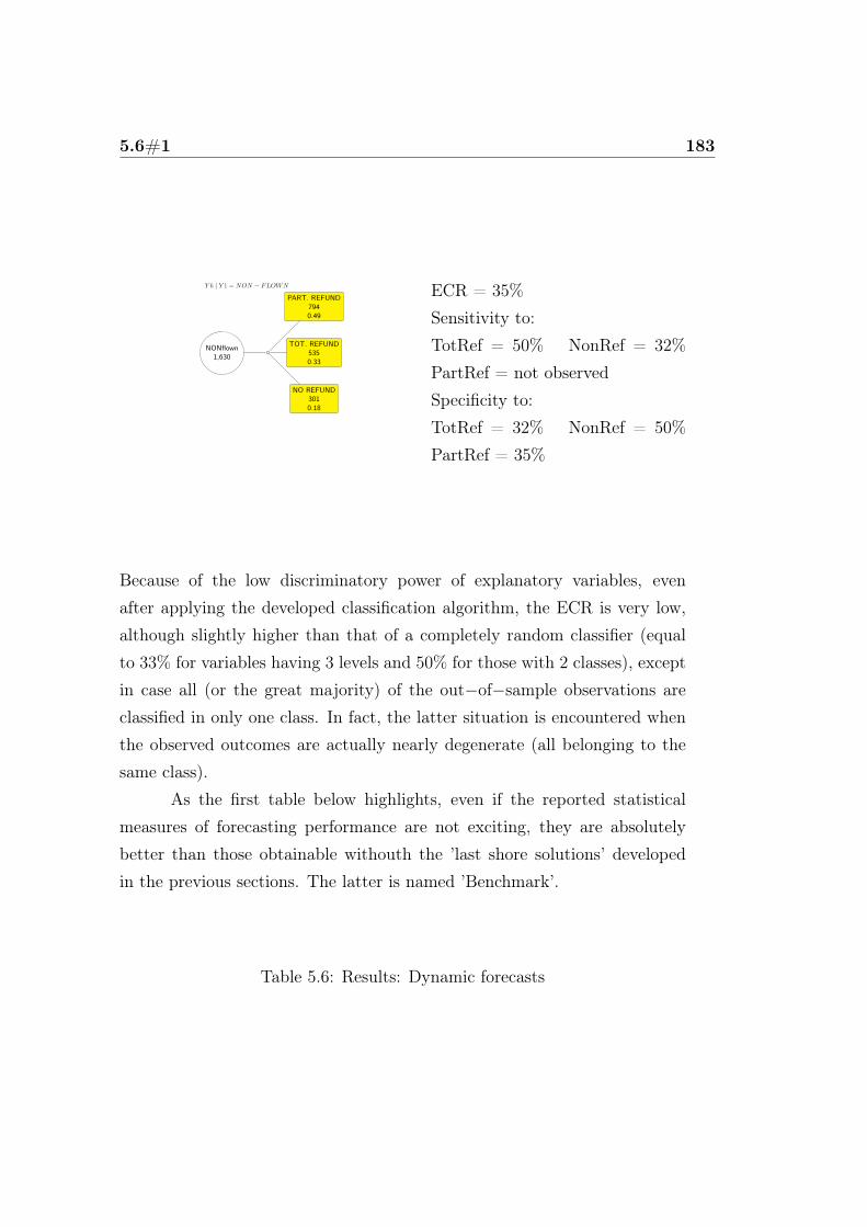
5.6#1 183
Y 6 | Y 1 = NON − FLOWN
NONflown1,630
NO REFUND3010.18
TOT. REFUND5350.33
PART. REFUND7940.49
ECR = 35%
Sensitivity to:TotRef = 50% NonRef = 32%
PartRef = not observedSpecificity to:TotRef = 32% NonRef = 50%
PartRef = 35%
Because of the low discriminatory power of explanatory variables, evenafter applying the developed classification algorithm, the ECR is very low,although slightly higher than that of a completely random classifier (equalto 33% for variables having 3 levels and 50% for those with 2 classes), exceptin case all (or the great majority) of the out−of−sample observations areclassified in only one class. In fact, the latter situation is encountered whenthe observed outcomes are actually nearly degenerate (all belonging to thesame class).
As the first table below highlights, even if the reported statisticalmeasures of forecasting performance are not exciting, they are absolutelybetter than those obtainable withouth the ’last shore solutions’ developedin the previous sections. The latter is named ’Benchmark’.
Table 5.6: Results: Dynamic forecasts

184 5.#1
FLOWN
NONfl
Ch
PARTIAL_CHANGE
TOT_CH
NON_REFUND
TOT_REFUND
TC_NONflown
TC_FLOWN
obs\pred FLOWN NON_REFUNDPARTIAL_CHANGETC_FLOWN TC_NONflownTOT_REFUND PART_REFUND tot
FLOWN 1,118 120 677 2,491 54 8 5 4,473
NON_REFUND 31 3 0 0 0 0 0 34
PARTIAL_CHANGE 455 0 16 0 0 0 0 471
TC_FLOWN 1,501 0 753 0 0 0 2,254
TC_NONflown 266 0 0 0 0 0 0 266
TOT_REFUND 4 0 0 0 0 4 0 8
tot 3,375 123 693 3,244 54 12 5 7,506
CORRECT 25% 9% 3% 33% 0% 50% NA 37%
100% 0% 0% 100%
In Dynamic Forecast Fashion
50% 32% 0% 100%
0% 100% 0% 100%
100% 2% 0% 100%
32% 50% 0% 100%
55% 25% 0% 100%
2% 100% 0% 100%
25% 55% 100% 0%
55% 37% 0% 100%
TO:Sensitivity Specificity
Sensitivity Specificity
BENCHMARK
In Static Forecast Fashion
BENCHMARK

5.6#1 185
The final leaves of the decision tree are written in bold font, in contrastto the intermediate nodes. The second table sumarizes the final results(in statistical terms) for the dynamic forecasts. The number of correctlyclassified outcomes, for each leaf, is colored in yellow. The red percentagesare the values of sensitivity to each class. Only the best performingpredictors are considered.
Predicted outcomes are listed by columns and observed ones by row.There is one extra column (Partial Refund) because this class is neverobserved in the forecasting sample, although it is forecasted quite often, asit was the most frequently observed one in the estimation sample.
The same considerations expressed for the performance of the staticpredictions hold also for the dynamic ones: these values should be readtaking into account the poor information available, the complexity of thephenomenon to be modeled and the improvement in forecasting accuracy,relatively to the original one, rather than in absolute terms.
However, the result that really matters for the present work is theeconomic one, which is quite satisfying: choosign which fare to buy based onthe predictions of Model 1A, after the proposed algorithm is applied, allowsa global saving of 109,011 euros, that represents approximately the 5% ofthe total cost of flights.

186 5.#1
Conclusions
This thesis was commissioned by a Travel Management Company (TMC),aiming at minimizing the overall cost of business flights it intermediates.The cost of a flight depends on various factors: the class on board, the route,the time of booking, the airline, that are chosen by the client company,but also by the eventual changes or renounce to the journey, made by thebusiness traveler, and by the fare: the only lever the TMC can operate.Thus, the objective of this work was to provide a statistical tool able to helpthe TMC choosing the optimal fare for each ticket, the one which, coeterisparibus, allows to make flights as cheap as possible.
Airlines offer fares with different levels of flexibility. The higher theprice of a fare, the lower the cost of eventual changes and waivers. Thus, theoptimal fare depends on the business traveler’s behavior, as he can changethe ticket, either partially or totally, fly the first issued ticket or renounceto the journey, eventually asking for a partial or total refund. How the flyerwill behave is highly uncertain, because in business environments travelerstend to undergo to events (changed meetings’ dates, epidemics or wars at thedestination, mechanical emergencies and so forth), as a qualitative study ofthe context highlighted. As a consequence, the natural statistical approachto this problem is deciding to buy the fare minimizing the expected value ofthe cost of each flight.
To compute the expected value of the cost of a flight it is necessaryto know the price of the ticket, the amount of the penalty for changes and
187

188 5.#1
the fare; and to estimate the probability of each addend. Unfortunately, thementioned data are missing in too many cases, in the available corporatedataset. Nonetheless, it is still possible to provide helpful indications,through the probability distribution of tickets’ outcomes (consequent tothe business traveler’s behavior). So the specific problem, addressed in thepresent work, was to try to predict if a traveler will fly the first issued ticketor opt for another alternative, of those listed above.
Analyzing the correlation structure between available data andperforming a qualitative study on a panel of frequent business flyers, itemerged that the tickets’ outcomes derive from the decision-making processof the traveler, rather than from the characteristics of tickets and flights.This evidence complicated the task, as most of the available data referexactly to such characteristics, instead than to those of the traveler, itscompany and alternative-specific variables, which would have been veryuseful. However, the phenomenon was modeled as a decision tree. It allowedto identify the models and to simplify the problem, through relations ofindependence from irrelevant alternatives, conditional to the parent node,at the cost of a progressive loss of efficiency, descending throughout thetree. For each node a variable is specified and modeled through a PureMultinomial Logit Model.
Due to the scarce correlation between the available variables andthe traveler’s behavior, the goodness of fit of estimated models is not verysatisfying, but the prediction performances are definitely worse. In fact, theExact Classification Ratio (ECR) of the models is either less than that ofa completely random guess, or very high, but for models predicting alwaysthe same (most often observed) outcome. This is the consequence of thepoor discriminatory power of independent variables, due to the fact that theavailable information is poor, especially in quality.
In fact, to predict the travelers’ behavior, alternative-specific andsubject related variables would be needed, but were unavailable or in-

5.6#1 189
sufficient in quantity, because the database was collected for purposesdifferent from that of the investigation. Moreover, it was not possible tospecify hierarchical models, because the sample is too unbalanced and manyobservations’ identifiers are missing and it is not sure that some of them donot belong to the identified ones’ groups. Furthermore, due to the 80/20rule of sales, most of the tickets are purchased for a few client companies, allwith the same characteristics, so same values of the explanatory variables,and, among many tickets, just very few are not flown after the first issuance.Besides, given that the dataset covers only one year, divided in estimationand forecasting sample, it was not possible to model time components.
In order to try to get useful predictors, even with the scarce relevantinformation available, some alternative solutions were proposed. A firsthint was searched in the literature and in the qualitative study of thephenomenon. They suggested that business travel follows a sort of seasonalpattern, tied to vacation periods. Thus, an attempt was made to insert aguess, for a vacation effect, directly in estimated models, because the guesswas not precise enough to exploit it within a Bayesian framework. Throughbootstrap, complete data were generated from the model augmented with theguess, to approximate the vacation effect as would have been estimated onsamples actually affected by it. Then the whole model was re-estimated oneach bootstrapped dataset and the averaged coefficients used for predictingnew bootstrapped data and the real forecasting sample.
Adding the guess about the vacation effect, all the models’ predictingcapability improved and it became possible to correctly classify some of thetwo most economically relevant outcomes. However statistical measures offorecasting performance do not matter as much as the economic result ofdecisions made as a function of predictions, in the present work. Whence theneed to develop a business-specific loss function, for evaluating predictiveperformances, given that the too many missing data about penalties andprices did not allow to estimate the expected value of the cost of flights
190 5.#1
through the models. The loss function is based on some assumptionssimplifying the very messy market of air ticket fares and compares theperformance of proposed predictors to that of a benchmark strategy. Thelatter consists in buying always the fixed fare.
Unfortunately, the value of such a loss function for the guess-basedpredictor is very unsatisfying. Therefore, a new classification algorithm,amplifying faint signals, exploiting the whole matrix of estimated probabili-ties, for each prediction, was developed. It is especially useful when a classis much more frequently observed than the most economically relevant ones,but also very flexible, as it can be applied to any matrix of probabilities,estimated by any classifier. Thanks to the proposed algorithm, the predictiveperformance of all the models improved and, although in statistical termsthe performances are still very low, in economic terms an estimated globalgain of 109,011 euros is obtained, through the selected predictor. Finally,predicting the two crucial nodes, the algorithm allowed to classify outcomesfollowing the first one.
However, a problem for selecting the best models for nodes two andfour emerged. In fact, after the application of the new algorithm, all thecandidate predictors displayed identical forecasting performance, as assessedthrough the traditional measures for nominal data. The latter are based onthe predicted outcomes, but do not consider the estimated probabilities ofeach outcome, that were different, in this case. Conditional probabilitiesare important, because one day the cost data could be available and theexpected value of the cost of flights computed. The reliability of suchexpectation will be higher the more accurate the estimated masses are.Thus, a further measure of forecasting accuracy, based on the probabilities,called Predictive Accuracy Score is proposed and employed.
The present work has important implications from the business travelmanagement perspective. In particular, it provided an initial and partial(as based on limited information) answer to a current topical question:
5.6#1 191
in business air travel, does ’best buy’ mean always choosing the cheapestticket? The reply appears to be: most of the time it does, but it is notalways the decision that minimizes the cost of flights. Based on the availableevidence, in the 85% of cases purchasing the cheapest fare allows to makegood saving. But 5% of the times it is more convenient to buy a refundableticket, otherwise the cost of the ticket is entirely lost, and for the 10% offlights a changeable fare is preferable to the more expensive purchase of anew ticket.
So, how can a corporate travel department know when a flexible fareis worth the higher price? The present work showed that it is possible toidentify some characteristics, of the traveler, of the company, of the flightand of the ticket, that influence the probability of ticket’s outcomes andreduce the uncertainty about this issue. It is also worth of noting thatinformation about the familiar and personal situation of the travelers wouldadd important clues, along with the identification of the flyer’s professionalstatus, that is known and can be modeled by corporate travel departments.Therefore, to the aim of minimizing the cost of flights, personalized corporatetravel policies can be more effective than an undifferentiated policy andthis research provided some useful methodologies in case of informativeproblems, that are not rare in corporate datasets.
Concluding, the present thesis made three original contributions tothe statistical methodology for predicting nominal data, in presence of poorinformation. First, a guess-based prediction technique, to exploit externalhints (available instead of prior information). Then a new classificationalgorithm, emphasizing the faint discriminatory power of scarcely correlatedexplanatory variables. Finally, the Predictive Accuracy Score. As informa-tive problems, of the kind encountered during this work, are not a rarity inbusiness statistics, there is room for possible future developments.
For example, it would be valuable to develop a more specific in-ferential test for the significance of differences in the Predictive Accuracy

192 5.#1
Scores of alternative models. More in general, it would be useful to testthe performances of the proposed solutions, and especially of the newclassification algorithm, in different fields, for instance in weather forecast,or to predict outstanding financial shocks. Finally, the basic ideas groundingthe proposed methods can be exploited in other directions, as they tendto extract as much relevant information as possible from nominal data, onwhich not many operations and computations can be done, because of theirqualitative and non-ordinal nature.
Bibliography
[1] Levere, J. (2000). Akturk , D., Gun, S., Kumuk , T. (2007). MultipleCorrespondence Analysis Technique Used in Analyzing the CategoricalData in Social Sciences. Journal of Applied Sciences. , 7, 585-588.
[2] Alam, S. S. and Yasin, N. M. (2010). What factors influence onlinebrand trust: evidence from online tickets buyers in Malaysia. Journalof theoretical and applied electronic commerce research. 5, 3.
[3] Alamdari, F. (2002). Regional development in airlines and travel agentsrelationship. Journal of Air Transport Management. 8, 339-348.
[4] American Express Travel. Amex investigations, retrievable from:https://travel.americanexpress.com/home.
[5] Andersen, P. and Gill, R. (1982). Cox’s regression model for countingprocesses, a large sample study. Annals of Statistics. 10, 1100-1120.
[6] Anderson, J. E. and Kraus, M. (1981). Quality of Service and theDemand for Air Travel. The Review of Economics and Statistics, 63(4),533-540.
[7] Arrow, R. D. (1963). Social Choice and Individual Values. 2nd Ed.New Haven: Yale University Press.
193
194 BIBLIOGRAPHY
[8] Baspunar, E. and Mendes, M. (2000). The usage of CorrespondenceAnalysis technique at the contingency tables. Journal of AgriculturalSciences. 6, 98-106.
[9] Bartke, P., Gorin, T., Walczak, D., Friedemann, M. (2012). Manag-ing Cancel & Rebook Behavior in Airline Revenue Management. Anapplication of fare adjustment techniques. Lufthansa Information Man-agement Passage. Lufthansa editions.
[10] Berger, V. W. and Exner, D. V. (1999). Detecting Selection Bias inRandomized Clinical Trials. Controlled Clinical Trials. August, 20, 4,319-327.
[11] Bitner, M. J. and Booms, B. H. (1982). Trends in Travel and TourismMarketing : The Changing Structure of Distribution Channels Journalof Travel Research. April, 20, 4, 39-44.
[12] Borenstein, S., and Rose, N.L. (1995). Bankruptcy and pricing behaviorin us airline markets. The American Economic Review. 85, 2, 397-402.
[13] Botimer, T., and Belobaba, P. (1999). Airline pricing and fare productdifferentiation: A new theoretical framework. Journal of the Opera-tional Research Society. 50, 11, 1085-1097.
[14] Brady, S.P., and Cunningham, W.A. (2001). Exploring predatory pric-ing in the airline industry. Transportation journal. 41, 1, 5-15.
[15] Brons, M., Pels, E., Nijkamp, P., and Rietveld, P. (2002). Price elastic-ities of demand for passenger air travel: a meta-analysis. Developmentsin Air Transport Economics, 8(3), 165-175.
[16] Chen, S. (2002). Differential pricing on the web: The case of online airtravel market. Business Economics and Public Policy. Kelley School ofBusiness, Indiana University.
BIBLIOGRAPHY 195
[17] Cheng, S. and Long, J. S. (2007). Testing for IIA in the MultinomialLogit Model. Sociological Methods & Research. May, 35, 4, 583-600.
[18] Clay, K., Krishnan, R., and Smith, M. (2001). The great experiment:Pricing on the internet. The handbook of electronic commerce in busi-ness and society. 139-152. Watson Eds, New York, CRC Press.
[19] Clemen, R. T. (1989). Combining forecasts: A review and annotatedbibliography. International Journal of Forecasting. 5, 559-583.
[20] Clemons, E.K., Hann, I.H., abd Hitt, L.M. (2002). Price dispersion anddifferentiation in online travel: An empirical investigation.ManagementScience. 48, 4, 534-549.
[21] Collins, D. and Tisdell, C. (2002). Gender and Differences in TravelLife Cycles. Journal of Travel Research. November, 41, 2, 133-143.
[22] Collins, D. and Tisdell, C. (2000). Travel Life Cycles Vary Significantlywith the Purpose of Travel. Department of Economics Discussion Pa-pers No. 276, University of Queensland, Brisbane.
[23] Cox D. R., Miller H. D. (1965). The Theory of Stochastic Pro-cesses.Chapman and Hall, London.
[24] Dilthey, W. (1883).Introduction to the Human Sciences. Princeton Uni-versity Press.
[25] Duzgunes, O., Kesici, T., Gurbuz, F. (1983). Statistical Methods I.Ankara Univeristy, Faculty of Agriculture Publications, 861.
[26] Flom, P. L. and Cassell, D. L. (2007). Stopping stepwise: Why step-wise and similar selection methods are bad, and what you should useNESUG Statistics and Data Analysis. 1-7.
196 BIBLIOGRAPHY
[27] Florens, J-P., FougÃĺre, D., Mouchart, M. (2008). Duration Modelsand Point Processes. The Econometrics of Panel Data: Handbook ofTheory and Applications. Eds. Sevestre P. and Lazlo M., 3rd edition,Springer, 547-601.
[28] Fossey, E., Harvey, C., McDermott, F., Davidson, L. (2002). Un-derstanding and evaluating qualitative research. Australian and NewZealand Journal of Psychiatry. November, 36, 6, 717-732.
[29] Foster, D. P. and Stine, R. A. (2006). Honest confidence intervals forthe error variance in stepwise regression. Working papers. The WhartonSchool of the University of Pennsylvania.
[30] Fourie, C., and Lubbe, B. (2006). Determinants of selection of full-service airlines and low-cost carriers−−A note on business travellers inSouth Africa. Journal of Air Transport Management, 12(2), 98-102.
[31] Freedman, D. A. (1983). A note on screening regression equations. TheAmerican Statistician. 37, 152-155.
[32] Fry, T. R. L. and Harris, M. N. (1996). A Monte Carlo study of tests forthe independence of irrelevant alternatives property.Journal of Trans-portation Research. 30, 1, 19-30.
[33] Gaudry, M. J. I. and Dagenais, M. G. (1979). The DOGIT model.Transportation Research. 13B, 2, 105-111.
[34] Gordon,S. C. and Smith, A. (2004).Quantitative Leverage ThroughQualitative Knowledge: Augmenting the Statistical Analysis of Com-plex Causes. Oxford Journals: Political Analysis. 12, 3, 223-255.
[35] Gorin, T., Walczak, D., Bartke, P., Friedemann, M. (2012). Incorporat-ing cancel and rebook behavior in revenue management optimization.Journal of Revenue and Pricing Management. 2, 117-126.

BIBLIOGRAPHY 197
[36] Graneheim, U. H. and Lundman, B. (2004). Qualitative content anal-ysis in nursing research: concepts, procedures and measures to achievetrustworthiness. Nurse Education Today. February, 24, 2, 105-112.
[37] Greenacre, M. J. (1984). Theory and Applications of CorrespondenceAnalysis. Academic Press, London.
[38] Guizzardi, A. (2002). La previsione economica. Problemi e metodistatistici. Guaraldi. Rimini.
[39] Harrell, F.E. (2001). with applications to linear models, logistic regres-sion, and survival analysis. Springer-Verlag, New York. Miller, A. J.(2002), Subset selection in regre
[40] Hausman, J. A. and McFadden, D. (1984). Specification tests for themultinomial Logit model. Econometrica. 52, 1219-1240.
[41] Horowitz, J. (1981) Identification and diagnosis of specification errorsin the multinomial Logit model. Transportation Research Record. 58,345-360.
[42] Huber, P. J. (1967). The Behavior of Maximum Likelihood Estimatesunder Nonstandard Conditions. Proceedings of the Fifth Berkeley Sym-posium on Mathematical Statistics and Probability. I, 221-33.
[43] Kim, L., Qu, H., Kim, D. J. (2009). A study of perceived risk andrisk reduction of purchasing air tickets online. Journal of Travel andTourism Marketing. 26, 3, 203-224.
[44] King, M. L. and Wu, P. X. (1993).Locally optimal one-sided tests formultiparameter hypotheses. Monash: Mimeo.
[45] Kulendran, N. and Wilson, K. (2000). Modelling business travelTourism Economics. 6, 1, 47-59.
198 BIBLIOGRAPHY
[46] Kulendran, N. and Witt, S. F. (2003). Forecasting the Demand forInternational Business Tourism. Journal of Travel Research. February, 41, 3, 265-271.
[47] Kruskal, W. H. (1960).Some Remarks on Wild Observations. Techno-metrics. 2,1, 1-3 .
[48] International Air Transport Association. (2000). Airline Economic Re-sults and Prospects, Part 1 Summary Report IATA.
[49] International Air Transport Association. (2014). Airline Economic Re-sults and Prospects, Part 1 Summary Report IATA.
[50] ISTAT. (2013). Rapporto Annuale. Il mercato del lavoro tra minori op-portunitÃă e maggiore partecipazione. Retrieved the 09/10/2014 from:http://www.istat.it/it/files/2013/05/cap3.pdf.
[51] L’osservatorio sul Business Travel. (2014). Turismo d’affari. Milano.Ediman.
[52] Law, R. and Chang, M. M. S. (2007). Online Pricing Practice of AirTickets: The Case of Hong Kong. Information and CommunicationTechnologies in Tourism. 513-522.
[53] Law, R. and Leung, R. (2000). A Study of Airlines’ Online ReservationServices on the Internet. Journal of Travel Research. November, 39, 2,202-211.
[54] Levere, J. (2000). Changing Roles. Airline Business. October, 48-76.
[55] Lin, P-C., Chen, C-C., Song, M-H. (2009). Price dispersion of onlineair tickets for short distance international routes The Service IndustriesJournal. 29, 11, 1597-1613.
[56] Luce, R. D. (1958). Individual Choice Behavior. New York: John Wiley.
BIBLIOGRAPHY 199
[57] Lukacs, P. M., Burnham, K. P., Anderson, D. R. (2010).Model selectionbias and FreedmanâĂŹs paradox. Annals of the Institute of StatisticalMathematics. 62, 117-125.
[58] Mason, K.J. and Gray, R. (1999). Stakeholders in a hybrid market: theexample of air business passenger trave European Journal of Marketing.33, 9/10, 844-858.
[59] Malterud, K. (2001). Qualitative research: standards, challenges, andguidelines. The Lancet. August, 358, 9280, 11, 483-488.
[60] McAfee, R. P. and Velde, V. (2006). Dynamic Pricing in the AirlineIndustry. Handbook on Economics and Information Systems. 1-43.
[61] McFadden, D., Tye, W. B., Train, K. (1978). An application of diagnos-tic tests for the independence from irrelevant alternatives property ofthe multinomial logit model. Transportation Research Record. January,637, 39-45.
[62] McFadden, D., Train, K.,Tye, W. B. (1981). An Application of Diag-nostic Tests for the Independence From Irrelevant Alternatives Prop-erty of the Multinomial Logit Model. Transportation Research BoardRecord. 637, 39-46.
[63] McNichols, M. and O’Brien, P. (1997). Self-Selection and Analyst Cov-erage. Journal of Accounting Research. Studies on Experts and theApplication of Expertise in Accounting, Auditing, and Tax. 35, 167-199.
[64] Moler, C. and van Loan, C. (2003). Nineteen Dubious Ways to Computethe Exponential of a Matrix, Twenty-Five Years Later. SIAM Review.45, 1, 3-49.

200 BIBLIOGRAPHY
[65] Nako, S. M. (1992). Frequent flyer programs and business travellers:An empirical investigation. Logistics and Transportation Review, 28(4),395-402.
[66] Nelder, J. A. and Mead, R. (1965). A simplex method for functionminimization. Computer Journal. 7, 308-313.
[67] Park, J. Y., and Jang, S. C. S. (2014). Sunk costs and travel cancella-tion: Focusing on temporal cost. Tourism Management. 40, 425−435.
[68] Proussaloglou, K., and Koppelman, F. S. (1999). The choice of aircarrier, flight, and fare class. Journal of Air Transport Management,5( 4), 193-201.
[69] Radner, R. and Marschak, J. (1954). Note on Some Proposed Deci-sion Criteria. In: R. M. Thrall, C. H. Coombs, R. L. Davies. DecisionProcess. New York, John Wiley.
[70] Ray, P. (1973). Independence of Irrelevant Alternatives. Econometrica.September, 41, 5, 987-991.
[71] Ritchie, JR.B. and Beliveau, D. (1974).Hallmark Events: An Eval-uation of a Strategic Response to Seasonality in the Travel Market.Journal of Travel Research. October, 13, 2, 14-20.
[72] Sauerbrei, W. (1999). The use resampling methods to simplify regres-sion models in medical statistics. Applied Statistics.48, 313-329.
[73] Shatland, E.S., Kleinman, K., Cain, E.M. (2008). A new strategy ofmodel building in PRO LOGISTIC with automatic variable selection,validation, shrinkage and model averaging. Proceeding of the twenty-ninth annual SAS users group international conference. 1-10.
[74] Levere, J. (1985). Small, K. A. and Hsiao, C. (1985). Multinomial Logitspecification tests. International Economics Review. 16, 471-486.

BIBLIOGRAPHY 201
[75] Steyerberg, E. W., Eijkemans, M. J. C., Harrell J., F. E., Habbema,J. D. F (2000). Prognostic modeling with logistic regression analysis:a comparison of selection and estimation methods in small data sets.Statistics in Medicine. 19, 1059-1079.
[76] Steyerberg, E. W., Eijkemans, M. J. C., Harrell J., F. E., Habbema,J. D. F. (2001). Prognostic modeling with logistic regression analysis:In search of a sensible strategy in small data sets. Medical DecisionMaking. 21, 45 -56.
[77] Swarbrooke, J. and Horner, S. (2001).Business Travel and Tourism.Butterworths-Heineman, London.
[78] Train, K. (2003).Discrete Choice Methods With Simulation. New York:Cambridge University Press.
[79] Train, K. Discrete Choice Methods with Simulation. (2009). CambridgeUniversity Press, second edition.
[80] Levere, J. (2000). Tse, Y. K. (1987) A diagnostic test for the multi-nomial Logit model. Journal of Business and Economic Statistics. 5,283-286.
[81] Tunstall, R. (1989). Catering for the female business traveller. Traveland Tourism Analyst. 5, 26-40.
[82] Venables, W. N. and Ripley, B. D. (2002). Modern Applied Statisticswith S. Fourth edition. Springer.
[83] Turismo dâĂŹaffari. (2014). Milano. Ediman.
[84] Vowles, T.M. (2000). The effect of low fare air carriers on airfares inthe US. Journal of Transport Geography. 8, 2, 121-128.
[85] Wallenberg, F. (2000). A study of airline pricing. Berkeley, CA: Uni-versity of California.
202 BIBLIOGRAPHY
[86] Wilfried, B. and Tarnai, C. (1999). Content analysis in empirical socialresearch. International Journal of Educational Research. January, 31,8, 659-671.
[87] Wunsch,G., Mouchart, M., Russo, F. (2014). Des Causes et des Effets.L’Academie en poche.
[88] Yoon, M. G., Yoon, D. Y., Yang, T. W. (2006). Impact of e-businesson air travel markets: Distribution of airline tickets in Korea. Journalof Air Transport Management. 12, 5, 253-260.