Predicting optimal solution cost with conditional …lelis/papers/2014/lelisSFZH14.pdfAbstract Heuristic search algorithms are designed to return an optimal path from a start state

Ann Math Artif IntellDOI 10.1007/s10472-014-9432-8

Predicting optimal solution cost with conditionalprobabilitiesPredicting optimal solution cost

Levi H. S. Lelis ·Roni Stern ·Ariel Felner ·Sandra Zilles ·Robert C. Holte

© Springer International Publishing Switzerland 2014

Abstract Heuristic search algorithms are designed to return an optimal path from a startstate to a goal state. They find the optimal solution cost as a side effect. However, thereare applications in which all one wants to know is an estimate of the optimal solutioncost. The actual path from start to goal is not initially needed. For instance, one might beinterested in quickly assessing the monetary cost of a project for bidding purposes. In suchcases only the cost of executing the project is required. The actual construction plan could beformulated later, after bidding. In this paper we propose an algorithm, named Solution CostPredictor (SCP), that accurately and efficiently predicts the optimal solution cost of aproblem instance without finding the actual solution. While SCP can be viewed as aheuristic function, it differs from a heuristic conceptually in that: 1) SCP is not requiredto be fast enough to guide search algorithms; 2) SCP is not required to be admissible; 3)our measure of effectiveness is the prediction accuracy, which is in contrast to the solutionquality and number of nodes expanded used to measure the effectiveness of heuristic func-tions. We show empirically that SCP makes accurate predictions on several heuristic searchbenchmarks.

Keywords Optimal solution cost prediction · Type systems · Heuristic search

Mathematics Subject Classifications (2010) 68T20 · 68W20 · 68W25

This work was carried out while L. H. S. Lelis was at the University of Alberta.

L. H. S. Lelis (�)Departamento de Informatica, Universidade Federal de Vicosa, Vicosa, Minas Gerais, Brazile-mail: [email protected]

R. Stern · A. FelnerInformation Systems Engineering, Ben Gurion University, Beer-Sheva, Israel

S. ZillesDepartment of Computer Science, University of Regina, Regina, SK, Canada

R. C. HolteComputing Science Department, University of Alberta, Edmonton, AB, Canada

mailto:[email protected]

L. H. S. Lelis et al.

1 Introduction

Heuristic search algorithms such as A* [11] and IDA* [17] are guided by the cost functionf (s) = g(s) + h(s), where g(s) is the lowest cost path known from the start state to s

and h(s), known as the heuristic function, is an estimate of the lowest cost path from s to agoal. A* and IDA* are designed to find a path from a start state to a goal state. They findthe solution cost as a side effect. However, there are applications in which all one wants isto know the optimal solution cost or an accurate estimate of the optimal solution cost – theactual path is not needed. For example, consider an owner of a construction company thatis required to quickly assess the monetary cost of a project for bidding purposes. In such acase, only the cost of executing the project is required. The actual construction plan couldbe formulated later, if the bid is won.

Thus, an important question to be answered is the following. Can we accurately andefficiently predict the optimal solution cost of a problem without finding a solution pathfrom the start to a goal? Korf et al. [22] stated: “Predicting the optimal solution cost for agiven problem instance (...) is an open problem”.

In this paper we present an efficient solution for this problem. We show empirically thatour method accurately predicts the optimal solution cost of problem instances in differentheuristic search benchmark domains. Our solution, named Solution Cost Predictor (SCP),is based on the prediction formula by Zahavi et al. [39], named Conditional DistributionPrediction (CDP), which predicts the number of nodes expanded on an iteration of IDA* fora given cost bound. We extend the ideas of Zahavi et al. to predict the optimal solution costof a problem instead of predicting the number of nodes expanded by IDA*.

The heuristic function h(s) used by heuristic search algorithms is in fact an estimate ofthe optimal solution cost. This estimate is called admissible if it never overestimates thecost of the lowest cost path from state s to the goal. This distinction is important, sinceheuristic search algorithms, such as A* and IDA*, guided by the cost function f = g + h

are guaranteed to find an optimal solution when h is admissible [11, 17]. A considerableamount of effort has been devoted to creating admissible heuristics [6, 13, 35, 38] andinadmissible heuristics [8, 14, 32, 36]. As shown in our experimental results, admissibleheuristics usually provide inaccurate predictions of the optimal solution cost as they arebiased to never overestimate the actual value. In some cases even inadmissible heuristicsare biased towards admissibility [8, 32].

Regardless of admissibility, heuristics share a property: the heuristic evaluation mustbe fast enough to be computed for every state generated during the search,1 while thesolution cost predictor is run only on the start state. In fact, often heuristic functionssacrifice accuracy for speed. By contrast, the algorithm presented in this paper aims ataccurately predicting the optimal solution cost of a problem instance. In summary, whileSCP can be viewed as a heuristic, it differs from a heuristic conceptually in that: 1) SCP isnot required to be fast enough to guide search; 2) SCP does not favor admissibility; 3) SCPaims at making accurate predictions and thus our measure of effectiveness is the predictionaccuracy, in contrast to the solution quality and number of nodes expanded used to measurethe effectiveness of heuristic functions.

1In some settings it is more efficient to perform heuristic calculation lazily during node expansion [31].

Predicting optimal solution cost with conditional probabilities

The paper is structured as follows. In Section 2, we describe in detail the CDP formulafor predicting the number of nodes expanded by IDA*, which is the basis of our predictionalgorithm. Section 3 presents SCP. Section 4 presents experimental results showing theaccuracy of the predictions made by SCP. In Section 5 we study empirically the parametersrequired by SCP. In Section 6 we mention additional applications of SCP. In Section 7 wediscuss the related work. Finally, in Section 8 we draw the concluding remarks of the workpresented in this paper.

This paper substantially extends a conference paper [24], which is to the best of ourknowledge the seminal work on efficiently predicting the optimal solution cost of individualproblem instances. In addition to a comprehensive explanation of the algorithm, we includenew experimental and theoretical results. We also include an empirical study of SCP’s inputparameters.

2 The CDP prediction framework

In this paper we use the term “search tree” of a search algorithm to refer to the nodesgenerated by that search algorithm until it halts. A node represents a unique state in thestate-space, and a state s might be represented by more than one node in a search tree, sincethere might exist more than one path from the start state to s. In addition, in contrast withstates, nodes have a g-cost and, if not the root of a search tree, nodes also have a parentnode. When clear from the context, we use the terms nodes and states interchangeably. Weassume unit-cost edges throughout.

The prediction algorithm presented in this paper is based on the CDP formula by Zahaviet al. [39]. In this section we introduce relevant notation and review CDP. Note that SCPpredicts the optimal solution cost, while CDP predicts the number of nodes expanded on aniteration of IDA* for a given cost bound.

2.1 Type systems

The CDP formula, as well as the SCP prediction algorithm presented in this paper, are basedon a partition of the nodes in a search tree named type system.

Definition 1 (Type system) Let S(s∗) be the set of nodes in the search tree rooted at s∗.T = {t1, . . . , tn} is a type system for S(s∗) if it is a disjoint partitioning of S(s∗). If s ∈S(s∗) and t ∈ T with s ∈ t , we write T (s) = t .

The accuracy of the CDP formula is based on the assumption that two nodes of the sametype root subtrees of the same size. IDA* with parent pruning will not generate a node s

from s if s is the parent of s. Therefore, because of parent pruning, the subtree below anode s differs depending on the parent from which s was generated. Zahavi et al. use theinformation about the parent of s when computing s’s type so that CDP is able to makeaccurate predictions of the number of nodes expanded by IDA* when parent pruning is used.

Definition 2 (Heuristic-preserving type system) A type system T is said to be heuristic-preserving if for every type, all nodes of that type have the same heuristic value. We thenwrite h(t) for any type t ∈ T to denote the heuristic value of the nodes of type t .


As in Zahavi et al.’s work, all type systems considered in this paper are heuristic-preserving.

Definition 3 Let t, t ′ ∈ T . p(t ′|t) denotes the average fraction of the children generated bya node of type t that are of type t ′. bt is the average number of children generated by a nodeof type t .

For example, if a node of type t generates 5 children on average (bt = 5) and 2 of themare of type t ′, then p(t ′|t) = 0.4. CDP samples the state space in order to estimate p(t ′|t)and bt for all t, t ′ ∈ T . CDP does its sampling as a preprocessing step and although typesystems are defined for nodes in a search tree rooted at s∗, sampling is done before knowingthe start state s∗. This is achieved by considering a state s drawn randomly from the statespace as the parent of nodes in a search tree. As explained above, due to parent-pruning,CDP uses the information about the parent of a node n when computing n’s type. Therefore,when estimating the values of p(t ′|t) and bt the sampling is done based on the children ofthe state s drawn randomly from the state space. We denote by π(t ′|t) and βt the respectiveestimates thus obtained. The values of π(t ′|t) and βt are used to estimate the number ofnodes expanded on an iteration of IDA*. The following example illustrates the predictionprocess.

Example 1 Consider the example in Fig. 1. Here, after sampling the state space to calculatethe values of π(t |u) and βu, we want to predict the number of nodes expanded on an iterationof IDA* with cost bound d for start state s0. We generate the children of s0, depicted in thefigure by s1 and s2, so that the types that will seed the prediction formula can be calculated.Given that T (s1) = u1 and T (s2) = u2 and that IDA* does not prune s1 and s2, the firstlevel of prediction will contain one node of type u1 and one of type u2, represented by thetwo upper squares in the right part of Fig. 1. We now use the values of π and β to estimatethe types of the nodes on the next level of search. For instance, to estimate how many nodesof type t1 there will be on the next level of search we sum up the number of nodes of type t1that are generated by nodes of type u1 and u2. Thus, the estimated number of nodes of typet1 at the second level of search is given by π(t1|u1)βu1 +π(t1|u2)βu2 . If h(t1)+2 (heuristicvalue of type t1 plus its g-cost) exceeds the cost bound d , then the number of nodes of typet1 is set to zero, because IDA* would have pruned those nodes. This process is repeated

Fig. 1 The first step of a CDP prediction for start state s0


for all types at the second level of prediction. Similarly, we get estimates for the third levelof the search tree. Prediction goes on until all types are pruned. The sum of the estimatednumber of nodes of every type is the estimated number of nodes expanded by IDA* withcost bound d for start state s0.

2.2 The CDP formula

Next, we describe the CDP prediction formula formally. Let child(n) be the set of childrenof node n in the search tree. The predicted number of nodes expanded by IDA* accordingto the CDP formula, for start state s∗, cost bound d , heuristic h, and type system T is asfollows.

CDP(s∗, d, h, T ) = 1 +∑

s∈child(s∗)

d∑

i=1

∑

t∈TN(i, t, s, d) . (1)

Here the first summation iterates over the nodes that seed the prediction formula; these arethe children of the start state s∗ (child(s∗)). In the example above, these nodes were s1 ands2. In the second summation we account for g-costs from 1 to the cost bound d , assumingnonnegative heuristic estimates; any value of i greater than d would be pruned by IDA*.The innermost summation iterates over the types in T . Finally, N(i, t, s, d) is the numberof nodes n of type t at level i of the subtree rooted at s. A value of one is added to 1 asCDP expands the start state so that the type of its children can be computed. N(i, t, s, d) iscomputed recursively as follows.

N(1, t, s, d) ={

0 if T (s) �= t ,

1 if T (s) = t .(2)

The case i = 1 is the base of the recursion and is calculated based on the types of thechildren of the start state. In the example in Fig. 1 N(1, t, s, d) is 1 only for types u1 andu2, and 0 for all other types in T . For i > 1,

N(i, t, s, d) =∑

u∈TN(i − 1, u, s, d)π(t |u)βu · Prune(t, i, d) . (3)

Here π(t |u)βu is the estimated number of states of type t a node of type u generates;Prune() is a pruning function that is 1 if the cost to reach a pair of type t plus the heuristiccost estimate of reaching the goal from there is less than or equal to the cost limit d , i.e.,Prune(t, i, d) = 1 if h(t)+ i ≤ d , and is 0 otherwise.

In summary, the CDP formula given above predicts the number of nodes expanded byIDA* with cost bound d , by predicting the number of nodes of each type generated byIDA* at every level of the search until the cost bound d . This is done incrementally. Firstthe number of nodes of each type at the first level of the search is given by the types ofthe children of the start state. The number of instances of each type is then estimated forthe second level of the search based on (3). This prediction process continues to deeper anddeeper levels until reaching the level of the cost bound d . The sum of the nodes of differenttypes at every level is an estimate of the total number of nodes predicted by CDP.

Zahavi et al. [39] introduced a method for improvingCDP predictions for a given probleminstance. Instead of directly predicting how many nodes will be expanded for cost boundd and start state s∗, all states at depth r < d , denoted by Cr , are generated and one thenpredicts how many nodes will be expanded for depth bound d − r with Cr as the set of


start states. We call this technique prediction lookahead, with r being the parameter thatdetermines the depth of the prediction lookahead. SCP also uses the prediction lookaheadto improve the accuracy of its predictions.

2.3 Different type systems

As defined above, a type system can be any partition over nodes of a search tree(Definition 1). Generally speaking, the type of node s can be any set of features of s. In thispaper we use domain-independent type systems defined using a given heuristic function, asdescribed next.

As our basic type system, Th, we use Zahavi et al.’s basic “two-step” model, defined(in our notation) as Th(s) = (h(parent(s)),h(s)), where parent(s) returns the node thatgenerated node s.

In addition, we also experimented with the following two type systems, which areextensions of the Th type system.

– Tc(s) = (Th(s), c(s, 0), . . . , c(s,H)), where c(s, k) is the number of children of s,considering parent pruning, whose h-value is k, and H is the maximum h-valueobserved in the sampling process;

– Tgc(s) = (Tc(s), gc(s, 0), . . . , gc(s,H)), where gc(s, k) is the number ofgrandchildren of s, considering parent pruning, whose h-value is k.

For instance, two nodes s and s ′ will be of the same Tc type (where c stands for children)if h(parent(s)) = h(parent(s ′)) and h(s) = h(s ′), and, in addition, s and s ′ generatethe same number of children with the same heuristic distribution. Similarly, two nodes s

and s ′ are of the same Tgc (where gc stands for grandchildren) type if besides matchingon the information required by the Tc type system, s and s ′ generate the same number ofgrandchildren with the same heuristic distribution. We specify and justify the choice of eachtype system used in our experiments in Section 4 below.

Recently, we identified a source of error in the CDP formula that had previously beenoverlooked [25]. We observed that “rare events” (i.e., low values of π(t |t ′)) could reduceCDP’s prediction accuracy. In addition, we presented a method that systematically disre-gards rare events, named ε-truncated CDP, that substantially improves prediction accuracy.In this paper we have also implemented ε-truncation as part of the solution cost predictionalgorithm described in the next section. We have empirically observed (see Section 5.3) thatε-truncation also improves the prediction accuracy of SCP.

2.4 Type systems are not abstractions

A common misconception is to think of type systems as state-space abstractions. Priedi-tis [30] defines a state-space abstraction as a simplified version of the problem in which(1) the cost of the least-cost path between two abstracted states must be less than or equalto the cost of the least-cost path between the corresponding two states in the original state-space; and (2) goal states in the original state-space must be goal states in the abstractedstate-space.

In contrast with state-space abstractions, a type system does not have these two require-ments. A type system is just a partition of the nodes in the search tree. It might noteven be possible to represent a type system as a graph since there might not be edgesconnecting types, a type system does not necessarily define the relation between the types.


However, note that abstractions also offer a partition of the nodes in the search tree. There-fore, although type systems may not be used as abstractions in some cases, abstractions canalways be used as type systems.

3 Solution cost predictor

We now describe the Solution Cost Predictor, SCP, a method based on CDP for estimatingthe optimal solution cost of state-space search problems.SCP requires the type system to have special types containing only goal nodes. We call

this kind of type a goal type, and define it as follows.

Definition 4 (Goal type) A type tg ∈ T is a goal type if for all nodes s ∈ tg , s is a goalnode.

During sampling, whenever we reach a state s, we perform a goal test on s. If s is a goal,then its type becomes a goal type. There can be as many goal types as different goal nodesin a search tree.

Type space We say that a type t generates a type t ′ if there exist two nodes s and s ′ such thats ∈ t , s ′ ∈ t ′, and s is the parent of s ′ in the search tree. We use the term type space to denotethe graph whose vertices are the types, and where every two types t and t ′ have a directededge between them if at least one node of type t generates at least one node of type t ′. Theweight of an edge between types t and t ′ in the type space is given by the probability of anode of type t generating a node of type t ′; note that these probabilities are the π(·|·)-valueslearned during CDP’s sampling.

3.1 The SCP prediction formula

Like CDP, SCP also samples the state space of a given problem with respect to a type systemas a preprocessing step to find the values of π(t |u) and βu (see Section 2). After sampling,SCP predicts the optimal solution cost for a given start state s∗ based on the values of π(t |u)and βu.

The basic building block of SCP is a formula for estimating the probability of at least onegoal node existing at a level of the search tree (a goal node n exists at level i of the searchtree rooted at s∗ if there is a path of cost i from s∗ to n). SCP estimates the probability ofa goal node existing at a level of search by approximating the probability of a node of agoal type existing at a level of search. This probability is estimated by extending the CDPprediction formula, as explained next.

The probability that a node of a goal type exists at the ith level of the search tree dependson (a) the probability that nodes exist at level i−1 that can potentially generate a goal node;and (b) the probability that at least one node at level i − 1 indeed generates a goal node. Ingeneral, we define p(i, t, s∗, d) as the approximated probability of finding at least one nodeof type t , in a search tree rooted at state s∗, at level i, with cost bound d . While computingp(i, t, s∗, d) we assume the variables π(·|·) to be independent.

Example 2 We now illustrate how p(i, t, s∗, d) is calculated with the example shown inFig. 2. Assume that only nodes of types t1, t2 and t3 can generate a node of type t4. In other


Fig. 2 Types at level i are used to calculate the approximated probability of t4 existing at level i + 1

words, for any type t �∈ {t1, t2, t3}, we have that π(t4|t) = 0. A node of type t4 exists at leveli + 1 iff at least one of the nodes of types t1, t2 or t3 at the previous level generates one ormore instances of the type t4.

We now describe exactly how p(i, t, s∗, d) is calculated. Let φ(M, t, t ′) be the probabil-ity of M nodes of type t generating no nodes of type t ′, assuming βt = 1. Given π(t ′|t), φis computed as follows.

φ(M, t, t ′) = (1 − π(t ′|t))MWe define p(i, t → t ′, s∗, d) as the approximated probability of one or more nodes of

type t existing at level i and generating at least one node of type t ′ at level i + 1. p(i, t →t ′, s∗, d) is calculated from p(i, t, s∗, d) and φ(N(i, t, s∗, d) · βt , t, t ′) as follows:

p(i, t → t ′, s∗, d) = p(i, t, s∗, d)(1 − φ(N(i, t, s∗, d) · βt , t, t ′)

)(4)

Recall that N(i, t, s∗, d) is the number of nodes of type t at level i of an IDA* search treerooted at s∗ with cost bound d . In 4 the term we subtract from 1 is the probability that noneof the N(i, t, s∗, d) · βt nodes generated by nodes of type t are of type t ′; this subtractiongives us the probability of at least one node of type t ′ being generated by nodes of type t .

Finally, p(i, t, s∗, d) can be formally defined as follows.

p(i, t, s∗, d) = 1 −∏

u∈T(1 − p(i − 1, u → t, s∗, d)) (5)

Here, the term 1 − p(i − 1, u → t, s∗, d) gives us the approximated probability of nonodes of type t being generated at level i by nodes of type u. By multiplying this probabilityfor every u in T we get the approximated probability of no nodes of type t being generatedat level i. Finally, when we subtract this resulting multiplication from 1 we get p(i, t, s∗, d),the approximated probability of there existing at least one node of type t at level i.

Note that (4) and (5) are recursive as p(i, t → t ′, s∗, d) depends on p(i, t, s∗, d), whichin turn depends on p(i − 1, u → t, s∗, d). The base of the recursion is defined for i = 1where we know exactly the probability of finding a node of a given type as this correspondsto the type of the children of the start state.

p(1, t, s∗, d) ={

1 if there exists a child s of s∗ such that T (s) = t ,

0 otherwise(6)

We write N(i, t), p(i, t → t ′), and p(i, t) instead of N(i, t, s∗, d), p(i, t → t ′, s∗, d),and p(i, t, s∗, d) whenever s∗ and d are clear from the context.

Next, we describe the SCP algorithm, which uses (5) presented above for estimating theprobability of an instance of type t existing at level i of a search tree bounded by cost d .


3.2 The SCP Algorithm

SCP predicts the optimal solution cost as follows:

1. First, set the cost bound d to the heuristic value of the start state.2. For every level i, estimate the probability of finding a goal type at that level in a search

tree bounded by cost d , using (5).3. Terminate returning d as the predicted optimal solution cost when a goal type exists at

level i with probability higher than a threshold value c provided by the user. Otherwise,increase the cost bound d by one and go to step 2.

SCP searches iteratively in the type space, incrementing the cost bound by one in case agoal type is not found with probability higher than c. This process is similar to how IDA*searches in the original state space. Algorithms 1 and 2 provide the pseudocode for SCP.The SCP algorithm starts in Algorithm 1. Initially, SCP uses the heuristic value of the startstate s∗ to initialize the cost bound d (line 1 of Algorithm 1). Initializing N(1, t) and p(1, t)(line 2) is done according to the children of the start state as shown in (2) and 6 for N(1, t)and p(1, t), respectively. N(1, t) is the number of nodes of type t among the children of s∗.p(1, t) is one if there is an instance of type t among the children of s∗, or zero otherwise.


For every level i (ranging from 2 to d), SCP calculates the values of N(i, t) and p(i, t)

of every type t by calling Algorithm 2 (line 6 of Algorithm 1). Algorithm 2 computes thevalues of N(i, t) as shown in line 7 and p(i, t) as shown in line 9. Algorithm 2 returnsp(i, t). Every node of type t at level i for a given cost bound d will be pruned by the searchif i+h(t) > d . Thus, in such cases we set N(i, t) and p(i, t) to zero (line 2 in Algorithm 2).

After every call to Algorithm 2 for a type t , if t is a goal type and p(i, t) is above theuser-defined threshold parameter c, the prediction halts and d is returned (line 8) as SCP’soptimal solution cost prediction. The reason SCP returns d and not i is explained in the nextsection.

3.3 Conditions for producing perfect predictions

In this section we show certain conditions in which SCP is guaranteed to produce perfectestimates of the optimal solution cost. First, we define a perfect type system and then weshow that SCP using such type system produces perfect predictions as long as each type issampled at least once.

Definition 5 (Perfect type system) A type system T is perfect if (i) every goal node has agoal type and (ii) for every t ∈ T , all nodes n ∈ t generate the same number of nodes andwith the same distribution of types.

Let T ∗ be a perfect type system, and C∗ the optimal solution cost.

Lemma 1 In SCP, for any type t and level i, N(i, t) > 0 ⇔ p(i, t) > 0

Proof We prove Lemma 1 by induction on i. In the base level (i=1), N(1, t) and p(1, t)are set according to the children of the initial state, i.e., N(1, t) and p(1, t) are both zero forall types except the types of the children of the initial state. Next, assume that Lemma 1 istrue for all i < n, and prove it for i = n.

We first prove that N(n, t) > 0 ⇒ p(n, t) > 0. Let t be a type for which N(n, t) > 0.Following Algorithm 2, we observe that N(n, t) is initialized to zero, and can only gainvalues larger than zero if there exists a type t ′ for which N(n − 1, t ′) · π(t |t ′)βt ′ > 0 (seeline 7). Both βt ′ and π(t |t ′) are non-negative, and thus N(n− 1, t ′) > 0. According to theinduction assumption, this entails that p(n − 1, t ′) > 0. Therefore p(n − 1, t ′ → t) > 0and p(n, t) > 0 as required.

Next, we proof the other direction, i.e., N(n, t) > 0 ⇐ p(n, t) > 0. If t is a type forwhich p(n, t) > 0, then there exists a type t ′ for which

p(n− 1, t ′) · (1 − φ(N(n− 1, t ′) · βt ′ , t, t ′)) > 0 (see line 9 of Algorithm 2)

1 − φ(N(n− 1, t ′) · βt ′ , t, t ′) > 0

(1 − π(t ′|t))N(n−1,t ′)·βt′ < 1

Since π(t ′|t), N(n− 1, t ′), and βt ′ cannot zero, then

1 − π(t ′|t) < 1 ∧ N(n− 1, t ′) · βt ′ > 0

π(t ′|t) > 0 ∧ N(n− 1, t ′) > 0 ∧ βt ′ > 0


According to Algorithm 2, N(n, t) ≥ π(t ′|t) · βt ′ · N(n − 1, t ′) (see line 7). Therefore,N(n, t) > 0 as required.

The computation of N(i, t), the number of states of type t predicted for level i, is exactlythe same as in CDP. Zahavi et al. [39] (Section 4.5.1) showed that with a perfect typesystem, and assuming that all types have been sampled (when constructing π and β), thenthe predictions of CDP are exactly correct.

Lemma 2 If SCP uses a perfect type system and every type has been sampled at least once,then there exists a goal type tg such that N(C∗, tg) > 0 and p(C∗, tg) > 0. In addition,N(i, t) = 0 and p(i, t) = 0 for any goal type t and every level i < C∗.

Proof Since C∗ is the optimal solution, at least one goal state must occur at depth C∗.Let tg be the type of that goal state. As the type system is perfect and all types have beensampled, CDP is exact, and thus N(C∗, tg) > 0 and following Lemma 1 p(C∗, tg) > 0.Similarly, there is no goal state at a depth lower than C∗. Thus, N(i, t) = 0 for any goaltype t and level i < C∗, and correspondingly p(i, t) = 0.

Theorem 1 (Perfect predictions) SCP using a perfect type system T ∗ produces perfectpredictions as long as each type in T ∗ is sampled at least once and the threshold value c isset to be zero.

Proof SCP halts when p(i, tg) > c, where tg is a goal type. From Lemma 2 we have thatp(i, tg) = 0 for any goal type if i < C∗. Thus, SCP would never underestimate. Also fromLemma 2 we have that there exists a goal type tg for which p(C∗, tg) > 0. Thus, SCP wouldalso not overestimate. Therefore, SCP produces perfect predictions.

3.4 The cost bound equality property of SCP

Next, we show that if a heuristic-preserving type system is based on a consistent heuristic,the value of i when SCP reaches line 8 of Algorithm 1 will always be equal to the currentcost bound d — we call this property the cost bound equality property.

Definition 6 Let u ∈ T and i, q ≥ 1. We say that type t ∈ T at level q cannot modify thevalue of p(i, u) if the computation of p(i, u) is independent of the value of N(q, t), i.e.,changes in N(q, t) do not affect the value of p(i, u).

Let T be a heuristic-preserving type system built from a consistent heuristic h(·). Further,let f (q, t) = q+h(t) where q is the level at which type t ∈ T is observed in the search tree.

Lemma 3 Let tg ∈ T be a goal type. Let i, q ≥ 1, i ≥ q . If f (q, u) > i for type u ∈ T atlevel q of the search tree, then u cannot modify the value of p(i, tg).

Proof Since T is a heuristic-preserving type system built from a consistent heuristic h(·),each type t ∈ T can only generate types t ′ (i.e., π(t ′|t) > 0) for which h(t ′) is one of thevalues h(t), h(t)+ 1, and h(t)− 1. In particular,

π(t ′|t) > 0 implies h(t ′) ≥ h(t)− 1 . (7)


Let f (q, u) > i. Suppose u can modify the value of p(i, tg). Thus, type u can gen-erate a goal type at level i. In particular, there must exist a type sequence of lengthi − q + 1, say (ti−q, ti−q−1, ti−q−2, · · · , t1, tg), such that ti−q = u and π(ti−q−1|ti−q) >

0, · · · , π(tg|t1) > 0. Since h(tg) = 0, (7) yields

h(u) = h(ti−q) ≤ h(tg)+ i − q = i − q .

The latter in turn implies f (q, u) = q+h(u) ≤ q+i−q = i in contradiction to f (q, u) > i.Hence u cannot modify the value of p(i, tg).

Theorem 2 If SCP uses a heuristic-preserving type system T built from a consistentheuristic h, then, for any value of c, the value of i in line 8 of Algorithm 1 is always equalto the current cost bound d .

Proof Let us first consider the case of the first iteration of the algorithm, when d = h(s∗).By analogy with the proof of Lemma 3, when replacing q by 0, there exists a sequence oftypes (ti , ti−1, · · · , t1, tg) such that π(ti−1|ti) > 0, · · · , π(tg|t1) > 0. Since h is consistent,(7) yields h(s) ≥ h(parent(s)) − 1 for every node s. Since h(tg) = 0, we obtain i ≥h(s∗) = d . Line 4 of Algorithm 1 implies i ≤ d = h(s∗), and thus i = d .

Next, consider the case d > h(s∗). During an iteration with d = U , SCP will expand allthe types that were expanded during the iteration with d = U − 1, and also the types u withf (u) = d that were not expanded in the previous iteration. Lemma 3 states that no typet with f (q, t) = U can modify the probability p(i, tg) for goal type tg at a level i < U .Therefore, for i = U−1, if SCP does not find a goal type tg with p(i, tg) ≥ c in the iterationwith d = U − 1, then SCP will not find a goal type tg with p(i, tg) ≥ c in the iteration withd = U either. So, for the test in line 7 of Algorithm 1 to be successful, i has to equal d .

3.4.1 Type systems based on inconsistent heuristics

If the type system is based on an inconsistent heuristic, Theorem 2 does not necessarilyhold. That is, type u ∈ T at level q of the search tree with f (q, u) > i can potentiallymodify the value of p(i, tg) for goal type tg . Thus, when using a type system built from aninconsistent heuristic, if returning i instead of d , Algorithm 1 could return a value smallerthan the current cost bound d . In fact, SCP could even return a value of i that is lower thanthe heuristic value of the start state.

Example 3 Consider the example shown in Fig. 3. Here we use the Th type system. Werepresent a type of a node n as tx,y , where x is the heuristic value of the parent of n, andy is the heuristic value of n. Figure 3a shows states and edges of two paths to the goal inthe original state space. The value in brackets in each circle is the heuristic value of thecorresponding state – note the heuristic inconsistency between nodes A and B, when theheuristic value changes by more than one (edge cost). Figure 3b shows the correspondingtypes for the states and edges shown in Fig. 3a. Now, assume that SCP is run on state A

from Fig. 3a. State A has a heuristic value of 6, and thus the optimal solution cost is at least6. However, SCP might return 3, since as shown in Fig. 3c there is a path of cost 3 in thetype space from type t7,6 – during sampling, SCP has seen a node of type t7,6 that generatesa node of type t6,2, which generates a node of type t2,1, and in a different part of the statespace SCP has sampled a node of type t2,1 that generates a goal node.


Fig. 3 States and edges in the original state space, their corresponding types in the type space, and a possible“shortcut” path in the type space

We have observed in our experiments that returning d instead of i in line 8 of Algorithm 1yields slightly more accurate predictions when the type system is built from an inconsistentheuristic.

3.5 Reducing the size of type systems built from inconsistent heuristics

We observed in our experiments that the number of types in a type space can be too largeto be practical when using an inconsistent heuristic. This is because, with an inconsistentheuristic, the number of different combinations of heuristic values in subtrees consideredin type systems such as Tc or Tgc is much larger than what is observed when a consistentheuristic is used. Recall that when the heuristic is consistent the heuristic value of nodesconnected by an edge in the search tree differ by at most one, when the heuristic is inconsis-tent, heuristic value of neighbor nodes might differ by any value, which increases the sizeof the Tc and Tgc type systems.

When using a type system that is very large, it may be difficult to sample properly alltypes. For example, a Tc type system for the 15-pancake puzzle was built based on theinconsistent heuristic that takes the maximum of the regular and the dual lookup of a PDB[10, 40]. Even after sampling 100 million random states and using biased sampling, therewere types that were not sampled.

We use a process similar to bidirectional pathmax (BPMX) [10] to shrink the size of typesystems based on inconsistent heuristics. This is done as follows. For every sampled states, the heuristic values of its children are increased by propagating the heuristic values fromother nodes while computing the type of s.

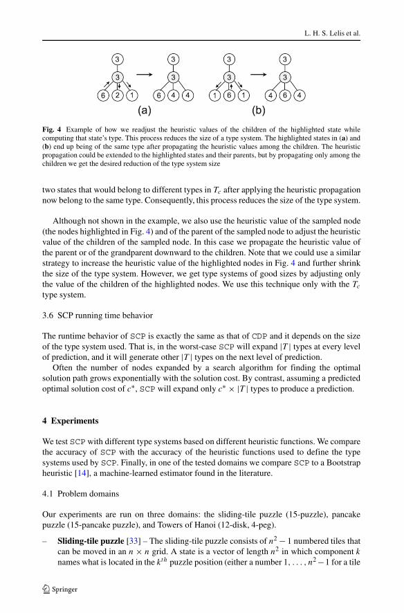
Example 4 Figure 4 illustrates this process. The children of the highlighted state in (a) withheuristic values of 2 and 1 can be raised to 4 as there is a child with heuristic value of 6.This is computed by subtracting the cost of the shortest path between the two siblings fromthe highest heuristic value among the children (6 − 2 = 4). The same process is applied tothe highlighted state in (b): the states with heuristic value of 1 can be raised to 4. Therefore,


Fig. 4 Example of how we readjust the heuristic values of the children of the highlighted state whilecomputing that state’s type. This process reduces the size of a type system. The highlighted states in (a) and(b) end up being of the same type after propagating the heuristic values among the children. The heuristicpropagation could be extended to the highlighted states and their parents, but by propagating only among thechildren we get the desired reduction of the type system size

two states that would belong to different types in Tc after applying the heuristic propagationnow belong to the same type. Consequently, this process reduces the size of the type system.

Although not shown in the example, we also use the heuristic value of the sampled node(the nodes highlighted in Fig. 4) and of the parent of the sampled node to adjust the heuristicvalue of the children of the sampled node. In this case we propagate the heuristic value ofthe parent or of the grandparent downward to the children. Note that we could use a similarstrategy to increase the heuristic value of the highlighted nodes in Fig. 4 and further shrinkthe size of the type system. However, we get type systems of good sizes by adjusting onlythe value of the children of the highlighted nodes. We use this technique only with the Tctype system.

3.6 SCP running time behavior

The runtime behavior of SCP is exactly the same as that of CDP and it depends on the sizeof the type system used. That is, in the worst-case SCP will expand |T | types at every levelof prediction, and it will generate other |T | types on the next level of prediction.

Often the number of nodes expanded by a search algorithm for finding the optimalsolution path grows exponentially with the solution cost. By contrast, assuming a predictedoptimal solution cost of c∗, SCP will expand only c∗ × |T | types to produce a prediction.

4 Experiments

We test SCP with different type systems based on different heuristic functions. We comparethe accuracy of SCP with the accuracy of the heuristic functions used to define the typesystems used by SCP. Finally, in one of the tested domains we compare SCP to a Bootstrapheuristic [14], a machine-learned estimator found in the literature.

4.1 Problem domains

Our experiments are run on three domains: the sliding-tile puzzle (15-puzzle), pancakepuzzle (15-pancake puzzle), and Towers of Hanoi (12-disk, 4-peg).

– Sliding-tile puzzle [33] – The sliding-tile puzzle consists of n2 − 1 numbered tiles thatcan be moved in an n × n grid. A state is a vector of length n2 in which component knames what is located in the kth puzzle position (either a number 1, . . . , n2−1 for a tile


Fig. 5 The goal state for the15-puzzle (left) and a state twomoves from the goal (right)

or a symbol representing the blank). Every operator swaps the blank with a tile adjacentto it. The left part of Fig. 5 shows the goal state that we used for the 15-puzzle while theright part shows a state created from the goal state by applying two operators, namelyswapping the blank with tile 1 and then swapping it with tile 5. The mean branchingfactor of the 15-puzzle is 2.1304 [22], and the average solution cost is 53 [19]. Thenumber of states reachable from any given state is (n2)!/2 [1].

– Pancake puzzle [7] – In the n-pancake puzzle, a state is a permutation of n numberedtiles and has n − 1 successors, with the lth successor formed by reversing the orderof the first l + 1 positions of the permutation (1 ≤ l ≤ n − 1). All n! permutationsare reachable from any given state. We report results for n = 15 which contains 15!reachable states. The upper part of Fig. 6 shows the goal state of the 15-pancake puzzle,while the lower part shows a state in which the first four positions have been reversed.The average solution cost of the 15-pancake puzzle is approximately 14.

– Towers of Hanoi [21] – The goal of this puzzle is to move all the disks from the originalposition onto a single peg. Only one disk can be moved at a time from the top of a pegonto another peg. A larger disk cannot be placed on top of a smaller disk. See Fig. 7for an example of the goal state of the Towers of Hanoi with 5 disks and 4 pegs. Weran experiments with the 12-disk and 4-peg Towers of Hanoi, which has 412 reachablestates from the goal state [21]. The average branching factor of the 4-peg Towers ofHanoi is about 3.766 [19].

4.2 Experimental setup

Parameter setting In all the experiments in this section we set the user-defined thresholdparameter c to 0.99. In Section 5.1 we empirically study the influence of different c-valueson the prediction accuracy. Analogously, in Section 5.2 we show empirically the effect ofdifferent r-values and in Section 5.3 the effect of ε-truncation in SCP’s prediction accuracy.

The depth of the prediction lookahead (i.e, the r-value shown in Section 2) was set to1 (r = 1) in most of the experiments in this section; on the 15-puzzle we also experimentwith r = 25. When experimenting with r > 1 we also make a prediction lookahead for theheuristic estimates, i.e., use the lowest heuristic value among the nodes at distance r fromthe start state. In Section 5.2 we show experiments with different values of r and we analyzehow this parameter affects the runtime and accuracy of SCP’s predictions.

Fig. 6 The goal state for the15-pancake puzzle (above) and astate one move from the goal(below)


Fig. 7 The 5-disk 4-peg Towersof Hanoi

Error measure We use the relative unsigned error to measure the prediction accuracy. Therelative unsigned error of an instance with optimal cost C and predicted cost P is |P−C|

C, i.e.,

the absolute difference between the predicted and the optimal cost, normalized by the opti-mal cost. A perfect score according to this measure is 0.00. Note that the relative unsignederror represents the percentage by which a predictor overestimates (or underestimates) theactual optimal solution cost. For instance, an error of 0.1 for a single prediction represents aprediction that overestimates (or underestimates) the optimal solution cost by 10 %. In ourplot of results we present the relative unsigned error in terms of percentage.

Results are presented in plots such as Fig. 8. The x-axis groups start states by theiroptimal solution costs and the y-axis represents the relative unsigned error of thepredictions. The error bars represent the 95 % confidence interval based on the assumptionthat the prediction error for a given optimal solution cost follows a normal distribution.

Type systems Ideally we would employ the Tgc type system in all our experiments as itstrictly contains more information than Tc and Th. However, depending on the domain andon the heuristic used, a Tgc type system can have a prohibitively large number of types,which prevents sampling of all types in a reasonable amount of time. Therefore, the choiceof the type system used in each experiment is closely related to (1) the heuristic functionused and also to (2) the problem domain. For instance, employing Tgc with an inconsistentheuristic for the 15-puzzle the size of the type system could become too large for samplingto be done in a reasonable amount of time. Usually inconsistent heuristics produce larger Tc

0

0.05

0.1

0.15

0.2

0.25

0.3

0.35

48 49 50 51 52 53 54 55 56

Re

lative

Un

sig

ne

d E

rro

r

Optimal Solution Cost

MD

DPDB

APDB

Bootstrap

SCP-MD

SCP-DPDB

SCP-APDB

Fig. 8 15-puzzle


and Tgc type systems as there is a larger variety of heuristic values among the children andgrandchildren of a node. The branching factor of a domain also influences the size of a typesystem. For instance, the 15-pancake puzzle, which has a much larger branching factor thanthe 15-puzzle, will likely have larger Tc and Tgc type systems due to the larger number ofheuristic values considered. The type system used in each experiment is specified below.

4.3 The sliding-tile puzzle

For the 15-puzzle we solved optimally and performed the SCP prediction for 1,000 randomsolvable states to measure prediction accuracy. To define π(t |u) and βt , one billion randomstates were sampled and, in addition, we use the biased sampling process introduced byZahavi et al. [39], in which we sample the child of a sampled state if the type of that childhad not yet been sampled.

Type systems Predictions with three different type systems were performed. We use thefollowing type systems/heuristic functions.

– Manhattan Distance (MD) – This is a popular and easy-to-implement heuristic functionfor the sliding-tile puzzles. It sums the Manhattan Distance of the individual tiles totheir goal position (excluding the blank tile). This heuristic is consistent and we use theTgc type system with it. The predictions using this type system will be referred to bySCP-MD.

– 7-8 Additive PDBs (APDB) – The 7-8 additive pattern database is an effective heuristicfor the 15 puzzle [9, 20]. It consists of the sum of two disjoint pattern databases, onebased on tiles 1-7 and the other based on tiles 8-15. The APDB is inconsistent2 and thetype system we use with it is the Tc type system. Predictions using this type system willbe referred to by SCP-APDB.

– Double Inconsistent PDB (DPDB) – This is the same heuristic used by [39]. Two PDBswere created, one based on tiles 1-7 and another one based on tiles 9-15. For states withthe blank in a location with an even number according to the goal state (see Fig. 5)the first PDB is consulted, the other PDB is consulted otherwise. As the blank alwayschanges from even to odd or odd to even from one state to a neighbor, the PDB that isconsulted alternates from parent to child. This generates inconsistency. The type systemwe use is Tc. Predictions using this type system will be referred to by SCP-DPDB.

In addition to comparing SCP predictions with the heuristics used to build the typesystems, we compare SCP predictions with the inadmissible Bootstrap heuristic [14]. TheBootstrap algorithm iteratively improves an initial heuristic function by solving a set ofsuccessively more difficult training problems in each iteration. This process was shown tocreate effective heuristics for a variety of domains [14, 36].

Figure 8 presents the results. First, the results show the well-known fact that theManhattan Distance (MD) heuristic is less accurate than the Additive PDB (APDB)heuristic. Second, SCP is able to produce accurate predictions, with errors less than 10 % ofthe optimal solution cost. Note that by comparison, all the tested admissible heuristics, MD,DPDB and APDB, tend to make inaccurate estimates, having an error of approximately30 %, 25 % and 15 %, respectively. This corresponds to the intuitive observation mentionedearlier in the paper that admissible heuristics tend to make poor estimates as they are biased

2See footnote 1 in [9]. We built the same PDBs.


0

0.05

0.1

0.15

0.2

0.25

0.3

0.35

48 49 50 51 52 53 54 55 56

Rela

tive U

nsig

ned E

rror


Bootstrap (r = 1)

Bootstrap (r = 25)

SCP-MD (r = 25)

SCP-DPDB (r = 25)

SCP-APDB (r = 25)

Fig. 9 15-puzzle (r=25)

to never overestimate the optimal cost. It is clear in this experiment that SCP using a typesystem based on a heuristic function produces more accurate predictions than the heuristicitself. We also observe in Fig. 8 that SCP’s prediction error is about half of Bootstrap’s forproblems with optimal solution cost of 51 or less.

According to the results shown in Fig. 8 the accuracy of the heuristic used to build a typesystem does not seem to affect SCP’s prediction accuracy much. SCP-MD, SCP-DPDB,and SCP-APDB are of similar accuracy, even though APDB is more accurate than MD andDPDB. While there is no definite explanation for this phenomenon, the results indicate thata type system does not necessarily have to be built from an accurate heuristic to allow SCPto make accurate predictions.

We also compare SCP’s prediction accuracy with the accuracy of Bootstrap when usingthe prediction lookahead. Figure 9 presents the results. For convenience we repeat the resultsof Bootstrap with no prediction lookahead (r=1) shown in Fig. 8. It is interesting to see thatthe prediction lookahead substantially reduces Bootstrap’s prediction accuracy. SCP, on theother hand, tends to benefit from the prediction lookahead as it is seeded with the exactdistribution of types at distance r from the start state. SCP-DPDB and SCP-APDB are moreaccurate than Bootstrap using either r = 1 or r = 25. In Section 5.2 we study the tradeoffbetween prediction accuracy and prediction runtime of the prediction lookahead.

4.4 The pancake puzzle

For the 15-pancake puzzle we use 1,000 random solvable states to measure predictionaccuracy. To define π(t |u) and βt , 100 million random states were sampled and, in addition,we use the biased sampling process described for the sliding-tile puzzle. In this experiment,in order to sample the goal types and states in the neighborhood of the goal types, 10,000out of the 100 million states sampled were generated with random walks of length 10 fromthe goal state.


0

0.05

0.1

0.15

0.2

0.25

0.3

12 13 14 15

Rela

tive U

nsig

ned E

rror


PDB

Dual-PDB

SCP-PDB

Weakened GAP

SCP-Weakened-GAP

GAP

SCP-Dual-PDB

Fig. 10 15-pancake puzzle

Type systems As with the 15-puzzle, we use three different heuristic functions to define thetype systems used in this experiment. The type systems used were based on the Tc typesystem.

– PDB – We created a PDB based on the location of the eight leftmost pancakes. Theresulting PDB is consistent. The predictions using this type system will be referred toby SCP-PDB.

– Dual-PDB – For this type system we use a heuristic that makes a regular and a duallookup on a PDB based on the leftmost eight pancakes and returns the maximum ofthem [10, 40]. The resulting heuristic is inconsistent. For the Dual-PDB there weretypes that were not sampled even after sampling 100 million random states. Thus, weused the process described in Section 3.5 to shrink the size of the type system so thatall types could be sampled at least once with 100 million random states.

– Weakened GAP – GAP is a very accurate hand-crafted consistent heuristic for the pan-cake puzzle [12].3 As the GAP heuristic already provides accurate cost estimates, it isnot interesting to build a type system for SCP with such an accurate heuristic. Thus, weuse a weakened version of it to build a type system. In our weakened version of GAPwe use the number of adjacent pancakes whose number differs by more than one exceptfor the rightmost pancake. We show the accuracy of GAP and its weakened version.

Figure 10 shows the results for the 15-pancake puzzle. As seen in the previous experi-ment, using SCP with a type system based on a given heuristic produces substantially moreaccurate predictions than using the heuristic itself as a predictor. This can be seen by thedifference between PDB and SCP-PDB, Dual-PDB and SCP-Dual-PDB, and WeakenedGAP and SCP-Weakened-GAP. SCP using a type system built from Dual-PDB is accurateand competitive with GAP.

3See also http://tomas.rokicki.com/pancake/

http://tomas.rokicki.com/pancake/


The results in Fig. 10 also show that the PDB based on the eight leftmost pancakes isthe least accurate estimator, giving estimates with errors of about 25 %. The type systembuilt with the consistent PDB clearly fails to offer a good partition of the state space. Asa consequence, SCP-PDB is the least accurate of the SCP predictions. SCP-Dual-PDB andSCP-Weakened-GAP on the other hand produce very accurate predictions – the errors indi-cate that the predictions are less than one move longer than the average optimal number ofmoves. Interestingly, SCP with Dual-PDB as well as SCP with Weakened GAP produce pre-dictions of similar accuracy even though the estimates of Dual-PDB are much less accuratethan the estimates of Weakened GAP.

4.5 Towers of hanoi

For the 12-disk 4-peg Towers of Hanoi we used 5,000 random solvable states to measureprediction accuracy. To define π(t |u) and βt , one million random states were sampled and,in addition, we used the biased sampling process previously described. Random instancesfor sampling were generated with random walks from the goal with a random lengthbetween 100 and 10,000 steps, while the random instances used to measure the accuracywere generated with random walks of fixed length of 500 steps.

Type systems We use two different type systems based on different PDB heuristics. In ourimplementation a state of the 12-disk 4-peg Towers of Hanoi is represented with 48 binaryvariables, one variable for each possible peg a disk might be on (12 for each of the 4 pegs).The variable vdp is set to one in a state if disk d is on peg p, and to zero otherwise. Theway we build simplified versions of the puzzle to create PDB heuristics is by projecting outsome of these variables. When we project out a variable vdp of a state we cannot distinguishwhether vdp carries a value of zero or one. The more variables we project out the more“simplified” will be the resulting puzzle. The choice of the PDBs we use for this domainin our experiments is arbitrary. That is, we arbitrarily selected two sets of variables to beprojected out so that we would have two different PDBs. The type system we use is Tgc .

– PDB1 – We created a PDB built by projecting out 20 of the 48 state variables. Namely,we project out the even disks from pegs 1 and 2, disks 2, 8, and 10 from peg 3, anddisks 2, 4, 6, 8, and 10 from peg 4. The resulting PDB is consistent. Predictions usingthis type system will be referred to by SCP-PDB1.

– PDB2 – We created another PDB by projecting out 19 of the 48 state variables. Namely,we projected out from pegs 1 and 2 the same disks we did for PDB1; from peg 3 weprojected out the same disks as in PDB1 with the exception of projecting out disk 8instead of disk 12; from peg 4 we also projected out the same disks as in PDB1, withthe exception of disk 10, which was not projected out.

Figure 11 shows the results for the Towers of Hanoi. The least accurate estimations ofthe solution cost are given by PDB1, followed by PDB2. A major improvement is observedwith the SCP predictions. For instance, the error drops from around 50 % to about 5 % whencomparing PDB2 with SCP-PDB2.

4.6 Discussion

There are several trends that are observed in all three domains. First, for every domainand every heuristic, using SCP with a given heuristic always produces predictions that aresubstantially more accurate than the heuristic used to build the type system. This shows the


0

0.1

0.2

0.3

0.4

0.5

0.6

0.7

0.8

13 14 15 16 17 18 19 20 21

Rela

tive U

nsig

ned E

rror


PDB1

PDB2

SCP-PDB1

SCP-PDB2

Fig. 11 12-disk 4-peg towers of hanoi

benefit of using SCP to predict the optimal cost over using heuristics. Furthermore, we haveobserved that SCP is able to make accurate predictions of the optimal solution cost evenwhen the type system being employed is built from an “inaccurate” heuristic function. Wehave also observed in some cases that SCP might produce inaccurate predictions, such asSCP-PDB1 in Fig. 11, where the error is about 30 % of the optimal solution cost. However,even in that case SCP is substantially more accurate than the heuristic function used to buildthe type system, which in that case produces estimates with errors of about 70 % of theoptimal solution cost.

4.7 SCP’s empirical running time

In this section we compare SCP’s and IDA*’s running time on the 15-puzzle. On thelefthand side of Table 1 we show the running time in seconds of both algorithms, as well asthe ratio between IDA*’s and SCP’s running time for problems with different solution costs(column “Cost” on the table). Ratio values larger than one mean that SCP is faster thanIDA* (e.g., a ratio of 27 means that SCP is 27 times faster than IDA*). We also present,on the righthand side of the table, the number of nodes expanded by each algorithm as wellas their ratio. Again, ratio values larger than one mean that SCP expands fewer nodes thanIDA*. It is important to show both running time and number of nodes expanded because thelatter is an implementation-independent measure.

The results on Table 1 show that IDA*’s running time and nodes expanded grow quicklywith the optimal solution cost. By contrast, SCP’s running time and number of nodesexpanded remain almost constant with the increase of the optimal solution cost. This dif-ference in the algorithms’ behavior is noted in the ratios, which increase with the optimalsolution cost. Finally, we remark that SCP can be substantially faster than IDA*, speciallyfor larger costs.


Table 1 SCP’s and IDA*’s running time in seconds and number of node expansions; average over 1,000problem instances of the 15-puzzle

Cost Running time Node expansions

IDA* SCP Ratio IDA* SCP Ratio

48 1.05 0.34 3.04 18,519,586 163,991 113

49 0.83 0.36 2.30 14,940,091 166,664 90

50 1.01 0.38 2.69 18,126,211 168,436 108

51 1.58 0.39 4.02 28,088,059 173,322 162

52 2.27 0.40 5.65 40,638,275 172,300 236

53 3.86 0.40 9.54 69,577,952 173,491 401

54 4.69 0.42 11.26 83,975,666 173,743 483

55 12.00 0.41 29.13 216,134,233 169,253 1,277

56 11.55 0.42 27.34 210,066,690 172,159 1,220

5 Empirical study of SCP’s parameters

In this section we make an empirical study of the parameters required by SCP. Namely, westudy the threshold parameter c, the prediction lookahead r , and the effects of ε-truncationon SCP’s prediction accuracy.

5.1 Empirical study of the threshold parameter

In Section 4 SCP was tested for a fixed set of parameters. Namely, we used a thresholdparameter c of 0.99. In this section we discuss the effect of this c-value on the accuracy of

0.02

0.03

0.04

0.05

0.06

0.07

0.08

0.09

0.1

48 49 50 51 52 53 54 55 56

Re

lative

Un

sig

ne

d E

rro

r


Fig. 12 Robustness to the parameter c for the 15-puzzle. SCP-MD


0.03

0.04

0.05

0.06

0.07

0.08

0.09

48 49 50 51 52 53 54 55 56

Rela

tive U

nsig

ned E

rror


Fig. 13 Robustness to the parameter c for the 15-puzzle. SCP-DPDB

SCP. We experimentally show the algorithm’s accuracy with a c-value of 0.80, 0.85, 0.90,0.95, and 0.99.

Figures 12, 13, and 14 present SCP’s prediction errors for different c-values for the 15-puzzle. Different curves correspond to different values of c. As can be observed, the effectof different c values is minor, and the curves are clustered together; there is no substantialdifference in prediction accuracy for the different c-values used. The accuracy of SCP is

0.04

0.05

0.06

0.07

0.08

0.09

0.1

48 49 50 51 52 53 54 55 56

Rela

tive U

nsig

ned E

rror


Fig. 14 Robustness to the parameter c for the 15-puzzle. SCP-APDB


relatively robust to the choice of c. Similar results were observed on the 15-pancake-puzzleand on the 12-disk 4-peg Towers of Hanoi.

5.2 Empirical study of the prediction lookahead

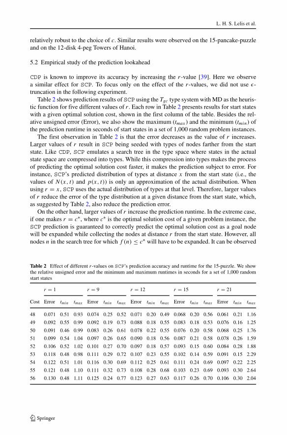
CDP is known to improve its accuracy by increasing the r-value [39]. Here we observea similar effect for SCP. To focus only on the effect of the r-values, we did not use ε-truncation in the following experiment.

Table 2 shows prediction results of SCP using the Tgc type system with MD as the heuris-tic function for five different values of r . Each row in Table 2 presents results for start stateswith a given optimal solution cost, shown in the first column of the table. Besides the rel-ative unsigned error (Error), we also show the maximum (tmax ) and the minimum (tmin) ofthe prediction runtime in seconds of start states in a set of 1,000 random problem instances.

The first observation in Table 2 is that the error decreases as the value of r increases.Larger values of r result in SCP being seeded with types of nodes farther from the startstate. Like CDP, SCP emulates a search tree in the type space where states in the actualstate space are compressed into types. While this compression into types makes the processof predicting the optimal solution cost faster, it makes the prediction subject to error. Forinstance, SCP’s predicted distribution of types at distance x from the start state (i.e., thevalues of N(x, t) and p(x, t)) is only an approximation of the actual distribution. Whenusing r = x, SCP uses the actual distribution of types at that level. Therefore, larger valuesof r reduce the error of the type distribution at a given distance from the start state, which,as suggested by Table 2, also reduce the prediction error.

On the other hand, larger values of r increase the prediction runtime. In the extreme case,if one makes r = c∗, where c∗ is the optimal solution cost of a given problem instance, theSCP prediction is guaranteed to correctly predict the optimal solution cost as a goal nodewill be expanded while collecting the nodes at distance r from the start state. However, allnodes n in the search tree for which f (n) ≤ c∗ will have to be expanded. It can be observed

Table 2 Effect of different r-values on SCP’s prediction accuracy and runtime for the 15-puzzle. We showthe relative unsigned error and the minimum and maximum runtimes in seconds for a set of 1,000 randomstart states

r = 1 r = 9 r = 12 r = 15 r = 21

Cost Error tmin tmax Error tmin tmax Error tmin tmax Error tmin tmax Error tmin tmax

48 0.071 0.51 0.93 0.074 0.25 0.52 0.071 0.20 0.49 0.068 0.20 0.56 0.061 0.21 1.16

49 0.092 0.55 0.99 0.092 0.19 0.73 0.088 0.18 0.55 0.083 0.18 0.53 0.076 0.16 1.25

50 0.091 0.46 0.99 0.083 0.26 0.61 0.078 0.22 0.55 0.076 0.20 0.58 0.068 0.25 1.76

51 0.099 0.54 1.04 0.097 0.26 0.65 0.090 0.18 0.56 0.087 0.21 0.58 0.078 0.26 1.59

52 0.106 0.52 1.02 0.101 0.27 0.70 0.097 0.18 0.57 0.093 0.15 0.60 0.084 0.28 1.88

53 0.118 0.48 0.98 0.111 0.29 0.72 0.107 0.23 0.55 0.102 0.14 0.59 0.091 0.15 2.29

54 0.122 0.51 1.01 0.116 0.30 0.69 0.112 0.25 0.61 0.111 0.24 0.69 0.097 0.22 2.25

55 0.121 0.48 1.10 0.111 0.32 0.73 0.108 0.28 0.68 0.103 0.23 0.69 0.093 0.30 2.64

56 0.130 0.48 1.11 0.125 0.24 0.77 0.123 0.27 0.63 0.117 0.26 0.70 0.106 0.30 2.04


that the maximum runtime when r = 21 is substantially higher than the other maximumruntimes.

However, contrary to common intuition, SCP is not fastest when r = 1. SCP makesquicker predictions for the r-values of 9, 12, and 15. The type system’s compression doesnot payoff for the first levels of search – the number of types is roughly the same as thenumber of nodes in the search tree and initially it is cheaper to expand the nodes in theactual state space rather than the types in the type space. The usage of types is advantageousonly when the number of nodes is substantially higher than the number of types.

5.3 Empirical study of ε-truncation with SCP

Next, we check the effect of ε-truncation on the accuracy of SCP predictions. Weisolate the effect of ε-truncation, in the subsequent experiment by setting the r-value to one.Table 3 shows the relative unsigned error of SCP with and without ε-truncation, on 1,000random 15-puzzle instances. Results are shown for each of the type systems described forthe 15-puzzle in Section 4. For convenience we drop the prefix “SCP” from the name ofthe type systems, and, in addition, we add an ε to the name of the type system if SCP usesε-truncation. We highlight an ε-truncation entry in the table if it is at least as accurate as itscounterpart.

As can be observed in Table 3, ε-truncation substantially improves the prediction accu-racy of SCP in the 15-puzzle. ε-truncation was designed to carefully ignore rare and harmfulevents observed during the CDP sampling. For instance, if a type t rarely generates a type t ′,then CDP improves its prediction accuracy by completely ignoring this rare event. The rareevents also seem to be harmful to SCP as carefully ignoring them improves SCP’s predic-tion accuracy. We conjecture that rare events create “shortcuts” to the goal type in the typespace, making SCP find the goal type prematurely (see [28] for details on ε-truncation).

In some domains the rare events are not observed, and in such domains ε-truncationdoes not change CDP’s prediction accuracy. We observed the same phenomenon in ourexperiments with SCP. ε-truncation does not change SCP’s prediction accuracy for the15-pancake puzzle and for Towers of Hanoi when using the heuristic functions describedabove. Moreover, like with CDP, ε-truncation has a larger impact on the SCP predictionsfor lower values of r .

Table 3 Effect of ε-truncation on SCP’s prediction accuracy for the 15-puzzle. The results with lowerprediction error are highlighted in bold

MD ε-MD DPDB ε-DPDB APDB ε-APDB

48 0.071 0.033 0.051 0.042 0.083 0.054

49 0.092 0.044 0.054 0.043 0.098 0.065

50 0.091 0.032 0.055 0.039 0.086 0.054

51 0.099 0.043 0.062 0.049 0.102 0.066

52 0.106 0.048 0.072 0.050 0.102 0.071

53 0.118 0.061 0.069 0.048 0.102 0.070

54 0.122 0.065 0.081 0.061 0.105 0.074

55 0.121 0.067 0.085 0.061 0.111 0.079

56 0.130 0.080 0.091 0.071 0.118 0.083


6 Possible applications of SCP

SCP could have other practical applications in addition to the merit of predicting the optimalsolution cost. Here are two possibilities.

Chenoweth and Davis [5] showed that by multiplying the heuristic estimates h(·) by asuitable constant w > 0 one could provably reduce the time complexity of a heuristic searchalgorithm using h(·) from exponential to polynomial in some problem domains. They alsosuggested a method for selecting a suitable value of w to “correct” the heuristic error andquickly find near-optimal solutions. The drawback of their method is that it requires prob-lem instances to be solved optimally. SCP predictions could be used to efficiently predictthe optimal solution cost of problem instances and thus find a weight that also “corrects”the heuristic error. Such w-value could be used with algorithms such as WIDA* [18] andWA* so that they quickly find near-optimal solutions.

Several search algorithms require an upper bound on the solution cost, e.g., Branch andBound [2] and Potential Search (PTS) [34]. PTS is a bounded-cost search algorithm thatefficiently searches for a solution with cost less than or equal to a given upper bound on thesolution cost. This is done by focusing the search on nodes that are more likely to lead to agoal with cost less than or equal to the desired bound. SCP can be used to find an accurateprediction of the optimal solution cost which is then multiplied by a weightw > 1 to providean upper bound for bounded cost search algorithms. In some cases the SCP prediction itselfrepresents an upper bound to the optimal solution cost. However, because SCP does notguarantee the predicted value to be an upper or lower bound to the optimal solution cost,multiplying the predicted value by w > 1 increases the chances of having an upper bound.

7 Related work

7.1 Search tree size predictors

SCP is based on CDP, a method developed for estimating the search tree size. The firstknown method for estimating the search tree size is due to Knuth [16]. Knuth’s methodworks by sampling a small portion of the search tree and from there inferring the total searchtree size. Under the mild assumption that the time required for expanding nodes is constantthroughout the search tree, an estimate of the size of the search tree provides an estimateof the search algorithm’s running time. Knuth noted that users of search algorithms usuallydoes not know a priori how long the search will take. Knuth’s method was later improvedby Chen [4] through the usage of a type system to reduce the variance of sampling. Wecall Chen’s method Stratified Sampling (SSS). Lelis [26] showed how to incorporate activesampling to SSS, further reducing the variance of sampling.

Independently of Knuth and Chen, Korf et al. [22] developed a method for estimatingthe size of the search tree expanded by IDA* [17]. Korf et al.’s method makes accuratepredictions of the IDA* search tree size for the special case of consistent heuristics. Zahaviet al.’s CDP generalized Korf et al.’s method to also produce accurate estimates of the IDA*search tree size when inconsistent heuristics are employed. Burns and Ruml extended CDPto work on domains with real-valued edge costs [3]. Lelis et al. presented a method calledε-truncation that mitigates a source of error that had been overlooked in CDP [25].SS and CDP have in common the usage of a type system to guide their sampling. Lelis et

al. [28] discovered that the type systems developed to be used with CDP could substantiallyimprove SSS’s prediction power. The main difference between SSS and CDP is that while


the former samples the search tree one wants to predict the size of, the latter samples theentire state space. Due to this difference in sampling strategy, as the number of samples growlarge, independently of the type system being used, SSS has the guarantee of producingperfect predictions, while CDP does not.

Knuth also noted in his seminal work that his method would not produce accuratepredictions of the size of the search tree expanded by branch and bound methods. Kilby etal. [15] developed methods that use the information seen during search to infer how manynodes branch and bound algorithm would expand. Similar approach was taken by Thayer etal. [37] to build a “progress bar” of best-first search variants. Lelis et al. [27] extended SSSinto a prediction algorithm they called Two-Step Stratified Sampling (TSS) and showedempirically on optimization problems over probabilistic graphical models [29] that TSS isable to produce good estimates of the size of the Depth-First Branch and Bound search tree.

7.2 Another solution cost predictor

Since SCP was first published, we developed another algorithm named BidirectionalStratified Sampling (BiSS) [23]. BiSS predicts the optimal solution cost of individualproblem instances by running a bidirectional search on the state space. It samples the statespace for each problem instance separately and it searches simultaneously from the start andthe goal. By contrast, in SCP the sampling of the original state space is performed only ina preprocessing phase, and the search is activated on the type space. The instance-specificsampling BiSS does allows it to scale to very large state spaces. However, BiSS also hasa few disadvantages. BiSS requires there to be a single goal state and is therefore notsuitable for domains in which a set of goal conditions is given instead of an actual goalstate. Another limitation is that BiSS is only applicable in domains in which it is possible toreason backwards from the goal. SCP is the algorithm of choice when only goal conditionsare given and also when it is not possible to reason backwards from the goal state.

8 Conclusions

In many real world scenarios it is sufficient to know the solution cost of a problem. Classicalsearch algorithms find the solution cost by finding an optimal path from the start to goal.Heuristic functions estimate the length of such a path, but are required to be fast enough tobe calculated for many nodes during the search.

In this paper we proposed SCP, an algorithm designed to accurately and efficiently pre-dict the optimal solution cost of a problem. While SCP can be viewed as a heuristic, itdiffers from a heuristic conceptually in that: 1) SCP is not required to be fast enough toguide search algorithms; 2) SCP does not favor admissibility; 3) SCP aims at making accu-rate predictions and thus our measure of effectiveness is the prediction accuracy, in contrastto the solution quality and number of nodes expanded used to measure the effectiveness ofother heuristic functions.

We showed empirically that SCP makes predictions with errors of less than 15 % ofthe optimal solution cost in all three domains tested. Our experiments also show that SCPwas always substantially more accurate than the heuristic functions used to build its typesystems. Moreover, SCP was consistently more accurate than the Bootstrap heuristic, amachine-learned inadmissible heuristic.

We also studied the impact of the parameters required by SCP on the prediction accuracy.Namely, we empirically studied the impact of the threshold parameter c, of the ε-cuts, and


of the prediction lookahead r on the prediction accuracy. Our results suggested that (1) forany value of c between 0.8 and 0.99 SCP makes accurate predictions; (2) ε-truncation cansubstantially improve the prediction accuracy; and (3) the prediction lookahead can improvethe prediction accuracy at the cost of increasing the runtime.

Acknowledgments This work was supported by the Laboratory for Computational Discovery at the Uni-versity of Regina. The authors gratefully acknowledge the research support provided by Alberta Innovates –Technology Futures, AICML, and NSERC.

References

1. Archer, A.F.: A modern treatment of the 15-puzzle. Am. Math. Mon. 106, 793–799 (1999)2. Balas, E., Toth, P.: Branch and bound methods. In: Lawler, E.L., Lenstra, J.K., Rinnooy Kart, A.H.G.,

Shmoys, D.B. (eds.) The Traveling Salesman Problem: A Guided Tour of Combinatorial Optimization.Wiley, New York (1985)

3. Burns, E., Ruml, W.: Iterative-deepening search with on-line tree size prediction. In: Proceedings of theInternational Conference on Learning and Intelligent Optimization, pp. 1–15 (2012)

4. Chen, P.-C.: Heuristic Sampling on Backtrack Trees. PhD thesis, Stanford University (1989)5. Chenoweth, S.V., Davis, H.W.: High performance A* search using rapidly growing heuristics. In:

International Joint Conference on Artificial Intelligence (1991)6. Culberson, J.C., Schaeffer, J.: Searching with pattern databases. In: Proceedings of the Canadian

Conference on Artificial Intelligence, volume 1081 of Lecture Notes in Computer Science, pp. 402–416.Springer (1996)

7. Dweighter, H.: Problem E2569. Am. Math. Mon. 82, 1010 (1975)8. Ernandes, M., Gori, M.: Likely-admissible and sub-symbolic heuristics. In: Proceedings of the European

Conference on Artificial Intelligence, pp. 613–617 (2004)9. Felner, A., Korf, R.E., Hanan, S.: Additive pattern database heuristics. J. Artif. Intell. Res. 22, 279–318

(2004)10. Felner, A., Zahavi, U., Schaeffer, J., Holte, R.C.: Dual lookups in pattern databases. In: Proceedings of

the International Joint Conference on Artificial Intelligence, pp. 103–108 (2005)11. Hart, P.E., Nilsson, N.J., Raphael, B.: A formal basis for the heuristic determination of minimum cost

paths. IEEE Trans. Syst. Sci. Cybern. SSC-4(2), 100–107 (1968)12. Helmert, M.: Landmark heuristics for the pancake problem. In: Proceedings of the Symposium on

Combinatorial Search, pp. 109–110. AAAI Press (2010)13. Helmert, M., Haslum, P., Hoffmann, J.: Flexible abstraction heuristics for optimal sequential planning.

In: Proceedings of the International Conference on Automated Planning and Scheduling, pp. 176–183(2007)

14. Jabbari Arfaee, S., Zilles, S., Holte, R.C.: Learning heuristic functions for large state spaces. Artif. Intell.175(16–17), 2075–2098 (2011)

15. Kilby, P., Slaney, J.K., Thiebaux, S., Walsh, T.: Estimating search tree size. In: Proceedings of the AAAIConference on Artificial Intelligence, pp. 1014–1019. AAAI Press (2006)

16. Knuth, D.E.: Estimating the efficiency of backtrack programs. Math. Comp. 29, 121–136 (1975)


17. Korf, R.E.: Depth-first iterative-deepening: An optimal admissible tree search. Artif. Intell. 27(1),97–109 (1985)

18. Korf, R.E.: Linear-space best-first search. Artif. Intell. 62(1), 41–78 (1993)19. Korf, R.E.: Linear-time disk-based implicit graph search. J. ACM 55(6), 26:1–26:40 (2008)20. Korf, R.E., Felner, A.: Disjoint pattern database heuristics. Artif. Intell. 134(1–2), 9–22 (2002)21. Korf, R.E., Felner, A.: Recent progress in heuristic search: A case study of the four-peg Towers of Hanoi

problem. In: Proceedings of the International Joint Conference on Artificial Intelligence, pp. 2324–2329(2007)

22. Korf, R.E., Reid, M., Edelkamp, S.: Time complexity of iterative-deepening-A∗. Artif. Intell. 129(1–2),199–218 (2001)

23. Lelis, L., Stern, R., Felner, A., Zilles, S., Holte, R.C.: Predicting optimal solution cost withbidirectional stratified sampling. In: Proceedings of the International Conference on Automated Planningand Scheduling, pp. 155–163. AAAI Press (2012)

24. Lelis, L., Stern, R., Jabbari Arfaee, S.: Predicting solution cost with condiditional probabilities.In: Proceedings of the Symposium on Combinatorial Search, pp. 100–107. AAAI Press (2011)

25. Lelis, L., Zilles, S., Holte, R.C.: Improved prediction of IDA*’s performance via ε-truncation.In: Proceedings of the Symposium on Combinatorial Search, pp. 108–116. AAAI Press (2011)

26. Lelis, L.H.S.: Active stratified sampling with clustering-based type systems for predicting the searchtree size of problems with real-valued heuristics. In: Proceedings of the Symposium on CombinatorialSearch, pp. 123–131. AAAI Press (2013)

27. Lelis, L.H.S., Otten, L., Dechter, R.: Predicting the size of depth-first branch and bound search trees.In: International Joint Conference on Artificial Intelligence, pp. 594–600 (2013)

28. Lelis, L.H.S., Zilles, S., Holte, R.C.: Predicting the size of IDA*’s search tree. Artif. Intell., 53–76 (2013)29. Pearl, J.: Probabilistic Reasoning in Intelligent Systems. Morgan Kaufmann (1988)30. Prieditis, A.E.: Machine discovery of effective admissible heuristics. Mach. Learn. 12(1–3), 117–141

(1993)31. Richter, S., Helmert, M.: Preferred operators and deferred evaluation in satisficing planning.

In: Proceedings of the International Conference on Automated Planning and Scheduling, pp. 273–280(2009)

32. Samadi, M., Felner, A., Schaeffer, J.: Learning from multiple heuristics. In: Proceedings of the AAAIConference on Artificial Intelligence, pp. 357–362. AAAI Press (2008)

33. Slocum, J., Sonneveld, D.: The 15 Puzzle. Slocum Puzzle Foundation (2006)34. Stern, R., Puzis, R., Felner, A.: Potential search: a bounded-cost search algorithm. In: Proceedings of the

International Conference on Automated Planning and Scheduling, pp. 234–241 (2011)35. Sturtevant, N.R., Felner, A., Barrer, M., Schaeffer, J., Burch, N.: Memory-based heuristics for explicit

state spaces. In: Proceedings of the International Joint Conference on Artificial Intelligence, pp. 609–614(2009)

36. Thayer, J., Dionne, A., Ruml, W.: Learning inadmissible heuristics during search. In: Proceedings of theInternational Conference on Automated Planning and Scheduling, pp. 250–257 (2011)

37. Thayer, J.T., Stern, R., Lelis, L.H.S.: Are we there yet? - estimating search progress. In: Proceedings ofthe 5th Annual Symposium on Combinatorial Search, pp. 129–136. AAAI Press (2012)

38. Yang, F., Culberson, J.C., Holte, R.C., Zahavi, U., Felner, A.: A general theory of additive state spaceabstractions. J. Artif. Intell. Res. 32, 631–662 (2008)

39. Zahavi, U., Felner, A., Burch, N., Holte, R.C.: Predicting the performance of IDA* using conditionaldistributions. J. Artif. Intell. Res. 37, 41–83 (2010)

40. Zahavi, U., Felner, A., Holte, R.C., Schaeffer, J.: Duality in permutation state spaces and the dual searchalgorithm. Artif. Intell. 172(4–5), 514–540 (2008)

Documents

Predicting optimal solution cost with conditional …lelis/papers/2014/lelisSFZH14.pdfAbstract Heuristic search algorithms are designed to return an optimal path from a start state