Embed Size (px)
Citation preview
PREDICTING PEAK OUTFLOW FROM BREACHED EMBANKMENT DAMS
Prepared for
National Dam Safety Review Board Steering Committee on Dam Breach Equations
Prepared by
M. W. Pierce, C. I. Thornton, and S. R. Abt
June 2010 Final
Colorado State University Daryl B. Simons Building at the
Engineering Research Center Fort Collins, CO
TABLE OF CONTENTS
1 INTRODUCTION...................................................................................................................1
2 BACKGROUND AND LITERATURE REVIEW...............................................................3 2.1 Simple-regression (Single-variable) Analysis ..................................................................8
2.1.1 Height of Water Behind the Dam (H).....................................................................8 2.1.2 Volume of Water Behind the Dam (V) ...................................................................9 2.1.3 Dam Factor (V·H) .................................................................................................10
2.2 Multiple-regression Analysis ..........................................................................................12
3 DATABASE EXPANSION...................................................................................................14
4 ANALYSIS OF H, V, WAVG AND L TERMS......................................................................... 4.1 Linear Regression (Qp and H) ............................................................................................. 4.2 Curvilinear Regression (Qp and H) ..................................................................................... 4.3 Linear Regression (Qp and V) ............................................................................................. 4.4 Linear Regression (Qp and V·H) ......................................................................................... 4.5 Linear Regression (Qp, V and H) ........................................................................................ 4.6 Linear Regression (Qp and Wavg) ........................................................................................4.7 Linear Regression (Qp and L).............................................................................................. 4.8 Multiple Regression (Qp, V, H and Wavg)............................................................................ 4.9 Multiple Regression (Qp, V, H and L)................................................................................. 4.10 Uncertainty Analysis 4.11 Comparison of Relationships 4.12 Case Study Comparison of Relations .................................................................................
5 CONCLUSIONS........................................................................................................................
6 REFERENCES..........................................................................................................................
i

LIST OF FIGURES
Figure 1 Artistic interpretation of the South Fork Dam breach ...................................................... 2
Figure 2 Peak outflow as a function of depth of water behind the dam
Figure 3 Peak outflow as a function of volume of water behind the dam ........................................
Figure 4 Peak outflow as a function of the dam factor (V·H) ...........................................................
Figure 5 Observed and predicted peak discharges using the Froehlich (1995) relationship ............
Figure 6 Plot of the 87 case studies in the composite database ........................................................
Figure 7 Comparison of the Equation 2 95% prediction interval, Equation 1 best-fit, and Reclamation (1982) envelope relationships...................................................................
Figure 8 Curvilinear-regression analysis of the composite database (Qp and H) .............................
Figure 9 Comparison of the Singh and Snorrason (1984), Evans (1986), and Equation 5 linear best-fit equations..................................................................................................
Figure 10 Comparison of the MacDonald and Langridge-Monopolis (1984), Costa (1985), and Equation 6 best-fit equations......................................................................
Figure 11 Observed and predicted peak discharges using the linear best-fit relationship expressed by Equation 7 ................................................................................................
Figure 12 Comparison of percent error for Equation 7 and the Froehlich (1995) relationship
Figure 13 Analysis of average embankment width (W ) as a peak-outflow predictor avg
Figure 14 Analysis of embankment dam length (L) as a peak-outflow predictor ............................
Figure 15 Observed and predicted peak discharges using the linear best-fit relationship expressed by Equation 9 ................................................................................................
Figure 16 Observed and predicted peak discharges using the linear best-fit relationship expressed by Equation 10 ..............................................................................................
ii

LIST OF TABLES
Table 1 Previous studies of peak-outflow prediction ..................................................................... 4
Table 2 Data collected from Wahl (1998) ...................................................................................... 6
Table 3Case studies reported by Pierce (2008).................................................................................
Table 4 Uncertainty summary...........................................................................................................
Table 5 Comparison of Froehlich (1995), Pierce (2008), VHL and VHW procedures for estimating peak flows ....................................................................................................
Table 6 Comparison of predictive relationships Table 7 Comparison of predicted peak outflow values and percent error
iii
LIST OF SYMBOLS, UNITS OF MEASURE, AND ABBREVIATIONS Symbols hd height of the dam hw height of the water behind the dam H height of the water behind the dam L dam length Qp peak outflow through the dam breach R2 coefficient of determination S reservoir storage V volume of water behind the dam Vw volume of water behind the dam at failure Vout volume of outflow through the breach during failure Wavg average dam width Wc dam crest width Zed downstream embankment slope
Units of Measure m meter(s) m3 cubic meter(s) m3/s cubic meter(s) per second m4 meter(s) to the fourth power % percent
Abbreviations FEMA Federal Emergency Management Agency FERC Federal Energy Regulatory Commission ICODS Interagency Committee on Dam Safety M&L-M MacDonald and Langridge-Monopolis Reclamation U. S. Bureau of Reclamation SCS Soil Conservation Service USACE U. S. Army Corps of Engineers USBR U. S. Bureau of Reclamation USDA-ARS U. S. Department of Agriculture - Agricultural Research Service
iv
1 INTRODUCTION
Construction of dams has been a long-established practice with the oldest known dam, the
Sadd el-Kafara near Cairo, Egypt, being built between 2950 and 2750 B.C. (Smith, 1971).
Historically, many of the early dams were small, in-channel structures built by locals with little or no
engineering background. Griffen (1974) suggests that dam safety for early dams was less of a concern
because the areas around early dams were less densely populated and, therefore, few people were
directly affected by the dams, these dams were generally small in relation to modern dams, and the
dams were generally built by cultures who took pride in their work.
Modern dam-safety analysis has been an evolving science since the 1970s. Between 1972 and
1977, four notable dam failures occurred in the United States: Buffalo Creek, West Virginia; Canyon
Lake, South Dakota; Teton, Idaho; and Kelly Barnes, Georgia. In April 1977, President Carter issued
a memorandum directing the review of federal dam-safety activities by a committee of recognized
experts. In June 1979, the Interagency Committee on Dam Safety (ICODS) issued its report
containing the first dam-safety guidelines for Federal agency dam owners.
Analysis of dam breaching and the resulting floods are essential to identifying and reducing
potential for loss of life and damage in the downstream floodplain. In recent years, computer
modeling has become available to simulate dam-break hydrographs and route these hydrographs
through the area downstream of the dam. Commonly used dam-break analysis programs require
estimates of certain geometric and temporal characteristics of the dam breach as inputs for the model.
Inundated areas, flow velocities, and flow depths can then be estimated to assess the potential damage
caused by the dam breach as portrayed in Figure 1.
1
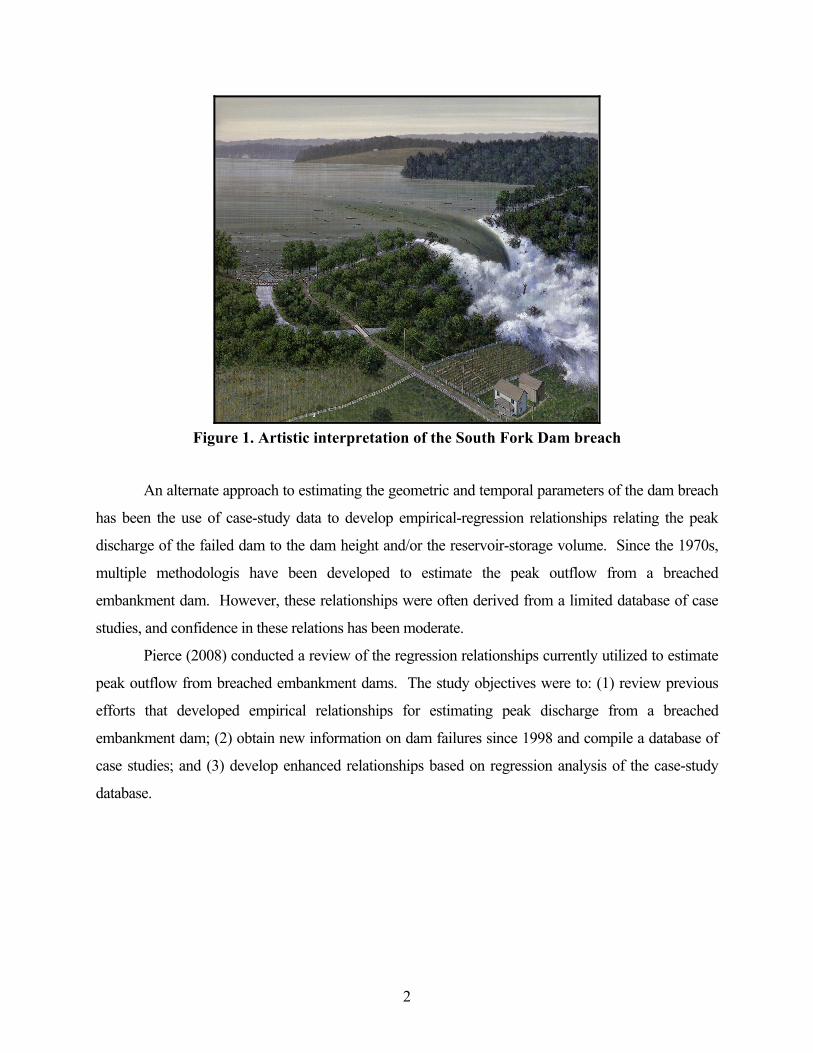
Figure 1. Artistic interpretation of the South Fork Dam breach
An alternate approach to estimating the geometric and temporal parameters of the dam breach
has been the use of case-study data to develop empirical-regression relationships relating the peak
discharge of the failed dam to the dam height and/or the reservoir-storage volume. Since the 1970s,
multiple methodologis have been developed to estimate the peak outflow from a breached
embankment dam. However, these relationships were often derived from a limited database of case
studies, and confidence in these relations has been moderate.
Pierce (2008) conducted a review of the regression relationships currently utilized to estimate
peak outflow from breached embankment dams. The study objectives were to: (1) review previous
efforts that developed empirical relationships for estimating peak discharge from a breached
embankment dam; (2) obtain new information on dam failures since 1998 and compile a database of
case studies; and (3) develop enhanced relationships based on regression analysis of the case-study
database.
2

2 BACKGROUND AND LITERATURE REVIEW
Many investigations have been conducted to develop methods used to predict the peak
discharge from a breached embankment dam. Most of these investigations have used simple-
regression analysis to relate the peak outflow through the breach to the depth of water behind the dam
at failure, the volume of water behind the dam at failure, or the product of the depth and volume. As
indicated in Table 1, the results of eleven (11) discreet investigations reported between 1977 and 1995
are presented to include the predictive expression, type of statistical curve fit, and number of case
studies used in the analysis. The variables in the relationships are: Qp = peak outflow (cubic meters
per second (m3/s)), hw = height of the water behind the dam at failure (m), hd = height of the dam (m),
S = reservoir storage at normal pool (m3), and Vw = volume of the water behind the dam at failure
(m3).
It is apparent that each investigator used slightly different terms to describe the effective head
and volume of water that created a breach through an embankment dam. Effective head has been
represented as both the height of the water behind the dam (hw) and the height of the dam (hd). The
volume of outflow through the breach has been represented as the volume of water behind the dam at
failure (Vw) and the reservoir storage (S). Additionally, definitions of reservoir storage vary for each
investigator. For example, Singh and Snorrason (1984) refer to the storage term as “reservoir storage
at normal pool,” and Costa (1985) describes volume as the reservoir volume at the time of failure.
Costa’s definition of volume does not include additional inflow during a flood and presumably could
include “dead storage” beneath the breach invert. Arguably, the best term to represent storage would
be a measurement of the volume of outflow through the breach during failure, but in many case
studies this has not been reported.
3
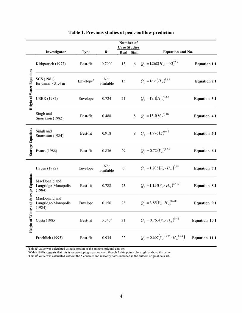
Table 1. Previous studies of peak-outflow prediction
Number of Case Studies
Investigator Type R2 Real Sim. Equation and No.
Kirkpatrick (1977) Best-fit 0.790a 13 6 ( ) 52302681 .wp .H.Q += Equation 1.1
Hei
ght o
f Wat
er E
quat
ions
SCS (1981) for dams > 31.4 m
Not Envelopebavailable 13 ( ) 85.16.16 wp HQ = Equation 2.1
( ) 85.11.19 wp HQ = Equation 3.1USBR (1982) Envelope 0.724 21
Singh and Snorrason (1982) Best-fit 0.488 8 ( ) 89.14.13 dp HQ = Equation 4.1
Stor
age
Equ
atio
ns
Singh and Snorrason (1984) Best-fit 0.918 8 ( ) 47.0776.1 SQp = Equation 5.1
( ) 53.072.0 wp VQ = Equation 6.1Evans (1986) Best-fit 0.836 29
Not Hagen (1982) Envelope available 6 ( ) 48.0205.1 wwp HVQ ⋅= Equation 7.1
Hei
ght o
f Wat
er a
nd S
tora
ge E
quat
ions
MacDonald and Langridge-Monopolis (1984)
Best-fit 0.788 23 ( ) 412.0154.1 wwp HVQ ⋅= Equation 8.1
MacDonald and Langridge-Monopolis (1984)
Envelope 0.156 23 ( ) 411.085.3 wwp HVQ ⋅= Equation 9.1
Costa (1985) Best-fit 0.745c 31 ( ) 42.0763.0 wwp HVQ ⋅= Equation 10.1
( )24.1295.0607.0 wwp HVQ ⋅= Equation 11.1Froehlich (1995) Best-fit 0.934 22
aThis R2 value was calculated using a portion of the author's original data set. bWahl (1998) suggests that this is an enveloping equation even though 3 data points plot slightly above the curve. cThis R2 value was calculated without the 5 concrete and masonry dams included in the authors original data set.
4
5
Wahl (1998, 2004) presented a database containing a composite of the case studies used by the
previous investigators to develop empirical relations for predicting dam-breach parameters and peak
discharge. Wahl used Vw, Vout, and S to represent different interpretations of the storage parameter
such that Vw and Vout were used to report data that fit specific definitions; where Vw = volume of water
stored above the breach invert at the time of failure, and Vout = volume of outflow through the breach
during failure. The term S was used when the definition of storage was less specific.
The Wahl (1998) database was comprised of 108 case studies, forty-three (43) entries
contained data describing the height (H) and volume (V) of water behind the dam at failure and an
estimate of the peak outflow (Qp) through the dam breach as presented in Table 2.
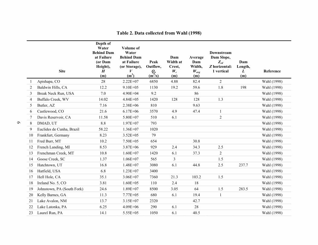
Table 2. Data collected from Wahl (1998)
Depth of Water
Behind Dam at Failure (or Dam Height),
Volume of Water
Behind Dam at Failure
(or Storage),
Downstream Dam Slope, Dam
Width at Crest,
Average Dam
Width, ZedPeak
Outflow, Dam
Length, Z horizontal: H V L Qp Wc Wavg Site 1 vertical Reference
(m3) (m3/s) (m) (m) (m) (m) 1 Apishapa, CO 28 2.22E+07 6850 4.88 82.4 2 Wahl (1998) 2 Baldwin Hills, CA 12.2 9.10E+05 1130 19.2 59.6 1.8 198 Wahl (1998) 3 Break Neck Run, USA 7.0 4.90E+04 9.2 86 Wahl (1998) 4 Buffalo Creek, WV 14.02 4.84E+05 1420 128 128 1.3 Wahl (1998) 5 Butler, AZ 7.16 2.38E+06 810 9.63 Wahl (1998) 6 Castlewood, CO 21.6 6.17E+06 3570 4.9 47.4 1 Wahl (1998) 7 Davis Reservoir, CA 11.58 5.80E+07 510 6.1 2 Wahl (1998) 8 DMAD, UT 8.8 1.97E+07 793 Wahl (1998)
6
9 Euclides de Cunha, Brazil 58.22 1.36E+07 1020 Wahl (1998) 10 Frankfurt, Germany 8.23 3.52E+05 79 Wahl (1998) 11 Fred Burr, MT 10.2 7.50E+05 654 30.8 Wahl (1998) 12 French Landing, MI 8.53 3.87E+06 929 2.4 34.3 2.5 Wahl (1998) 13 Frenchman Creek, MT 10.8 1.60E+07 1420 6.1 37.3 2 Wahl (1998) 14 Goose Creek, SC 1.37 1.06E+07 565 3 1.5 Wahl (1998) 15 Hatchtown, UT 16.8 1.48E+07 3080 6.1 44.8 2.5 237.7 Wahl (1998) 16 Hatfield, USA 6.8 1.23E+07 3400 Wahl (1998) 17 Hell Hole, CA 35.1 3.06E+07 7360 21.3 103.2 1.5 Wahl (1998) 18 Ireland No. 5, CO 3.81 1.60E+05 110 2.4 18 Wahl (1998) 19 Johnstown, PA (South Fork) 24.6 1.89E+07 8500 3.05 64 1.5 283.5 Wahl (1998) 20 Kelly Barnes, GA 11.3 7.77E+05 680 6.1 19.4 1 Wahl (1998) 21 Lake Avalon, NM 13.7 3.15E+07 2320 42.7 Wahl (1998) 22 Lake Latonka, PA 6.25 4.09E+06 290 6.1 28 Wahl (1998) 23 Laurel Run, PA 14.1 5.55E+05 1050 6.1 40.5 Wahl (1998)
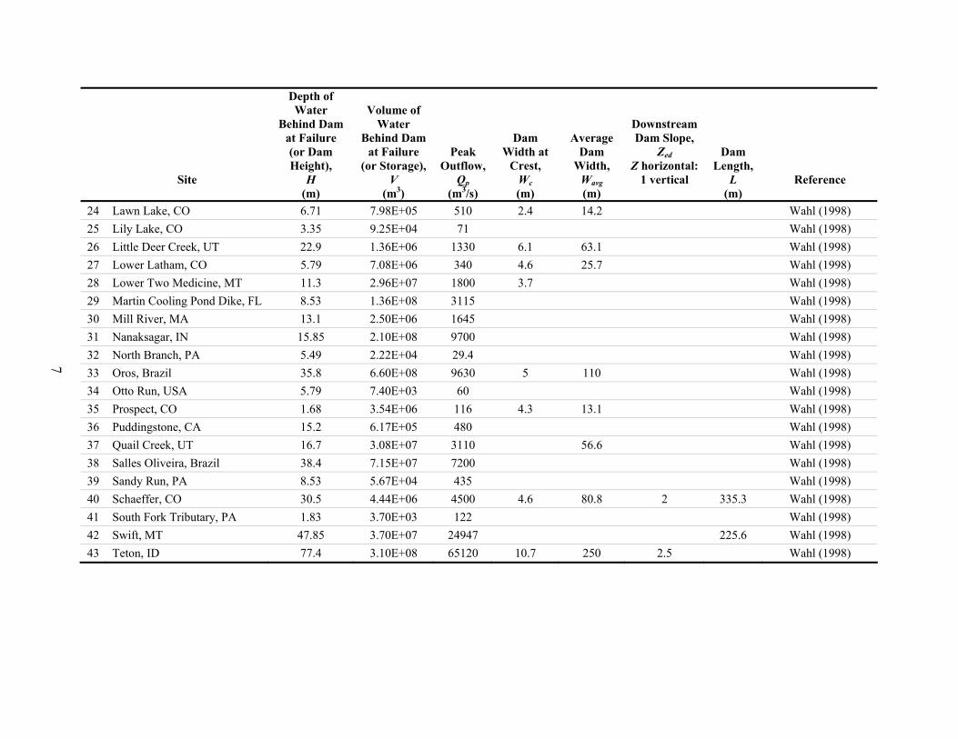
Site
Depth of Water
Behind Dam at Failure (or Dam Height),
H (m)
Volume of Water
Behind Dam at Failure
(or Storage), V
(m3)
Peak Outflow,
Qp(m3/s)
Dam Width at
Crest, Wc(m)
Average Dam
Width, Wavg(m)
Downstream Dam Slope,
ZedZ horizontal:
1 vertical
Dam Length,
L (m)
Reference
24 Lawn Lake, CO 6.71 7.98E+05 510 2.4 14.2 Wahl (1998) 25 Lily Lake, CO 3.35 9.25E+04 71 Wahl (1998) 26 Little Deer Creek, UT 22.9 1.36E+06 1330 6.1 63.1 Wahl (1998) 27 Lower Latham, CO 5.79 7.08E+06 340 4.6 25.7 Wahl (1998) 28 Lower Two Medicine, MT 11.3 2.96E+07 1800 3.7 Wahl (1998) 29 Martin Cooling Pond Dike, FL 8.53 1.36E+08 3115 Wahl (1998) 30 Mill River, MA 13.1 2.50E+06 1645 Wahl (1998) 31 Nanaksagar, IN 15.85 2.10E+08 9700 Wahl (1998) 32 North Branch, PA 5.49 2.22E+04 29.4 Wahl (1998) 33 Oros, Brazil 35.8 6.60E+08 9630 5 110 Wahl (1998) 34 Otto Run, USA 5.79 7.40E+03 60 Wahl (1998) 35 Prospect, CO 1.68 3.54E+06 116 4.3 13.1 Wahl (1998) 36 Puddingstone, CA 15.2 6.17E+05 480 Wahl (1998) 37 Quail Creek, UT 16.7 3.08E+07 3110 56.6 Wahl (1998) 38 Salles Oliveira, Brazil 38.4 7.15E+07 7200 Wahl (1998) 39 Sandy Run, PA 8.53 5.67E+04 435 Wahl (1998) 40 Schaeffer, CO 30.5 4.44E+06 4500 4.6 80.8 2 335.3 Wahl (1998) 41 South Fork Tributary, PA 1.83 3.70E+03 122 Wahl (1998) 42 Swift, MT 47.85 3.70E+07 24947 225.6 Wahl (1998)
2.5 250 10.7 65120 3.10E+08 77.4
7
Teton, ID 43 Wahl (1998)
2.1 Simple-regression (Single-variable) Analysis The majority of previous investigations have used case-study data to develop empirical
equations relating peak-breach discharge to the height of water behind the dam, volume of water
behind the dam, or the product of the height and volume. Single-variable linear regression models
were fit to case-study data to develop the following relationships.
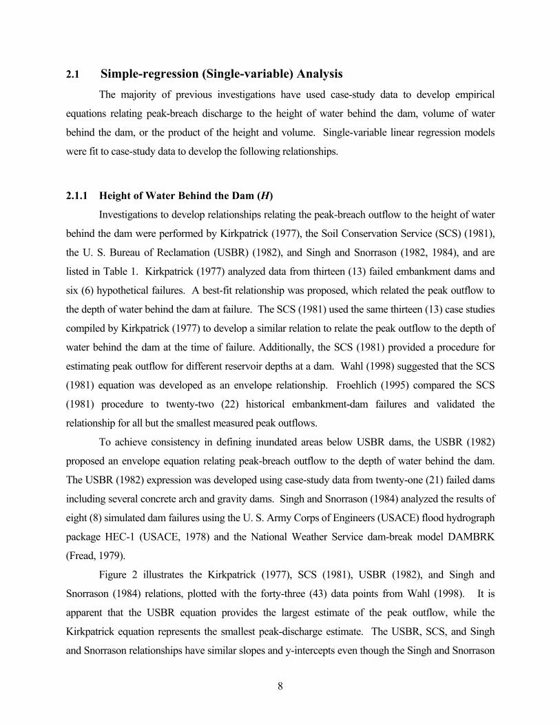
2.1.1 Height of Water Behind the Dam (H)
Investigations to develop relationships relating the peak-breach outflow to the height of water
behind the dam were performed by Kirkpatrick (1977), the Soil Conservation Service (SCS) (1981),
the U. S. Bureau of Reclamation (USBR) (1982), and Singh and Snorrason (1982, 1984), and are
listed in Table 1. Kirkpatrick (1977) analyzed data from thirteen (13) failed embankment dams and
six (6) hypothetical failures. A best-fit relationship was proposed, which related the peak outflow to
the depth of water behind the dam at failure. The SCS (1981) used the same thirteen (13) case studies
compiled by Kirkpatrick (1977) to develop a similar relation to relate the peak outflow to the depth of
water behind the dam at the time of failure. Additionally, the SCS (1981) provided a procedure for
estimating peak outflow for different reservoir depths at a dam. Wahl (1998) suggested that the SCS
(1981) equation was developed as an envelope relationship. Froehlich (1995) compared the SCS
(1981) procedure to twenty-two (22) historical embankment-dam failures and validated the
relationship for all but the smallest measured peak outflows.
To achieve consistency in defining inundated areas below USBR dams, the USBR (1982)
proposed an envelope equation relating peak-breach outflow to the depth of water behind the dam.
The USBR (1982) expression was developed using case-study data from twenty-one (21) failed dams
including several concrete arch and gravity dams. Singh and Snorrason (1984) analyzed the results of
eight (8) simulated dam failures using the U. S. Army Corps of Engineers (USACE) flood hydrograph
package HEC-1 (USACE, 1978) and the National Weather Service dam-break model DAMBRK
(Fread, 1979).
Figure 2 illustrates the Kirkpatrick (1977), SCS (1981), USBR (1982), and Singh and
Snorrason (1984) relations, plotted with the forty-three (43) data points from Wahl (1998). It is
apparent that the USBR equation provides the largest estimate of the peak outflow, while the
Kirkpatrick equation represents the smallest peak-discharge estimate. The USBR, SCS, and Singh
and Snorrason relationships have similar slopes and y-intercepts even though the Singh and Snorrason
8
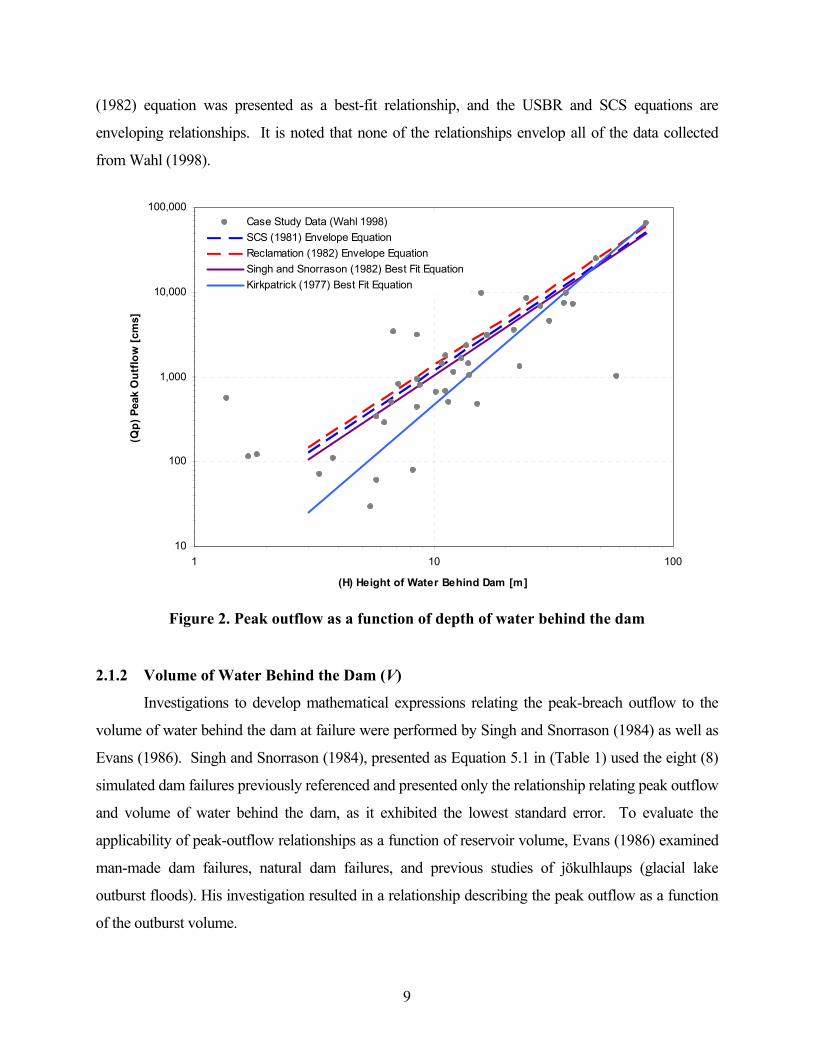
(1982) equation was presented as a best-fit relationship, and the USBR and SCS equations are
enveloping relationships. It is noted that none of the relationships envelop all of the data collected
from Wahl (1998).
10
100
1,000
10,000
100,000
1 10
(H) Height of Water Behind Dam [m]
(Qp)
Pea
k O
utflo
w [c
ms]
100
Case Study Data (Wahl 1998)SCS (1981) Envelope EquationReclamation (1982) Envelope EquationSingh and Snorrason (1982) Best Fit EquationKirkpatrick (1977) Best Fit Equation
Figure 2. Peak outflow as a function of depth of water behind the dam
2.1.2 Volume of Water Behind the Dam (V)
Investigations to develop mathematical expressions relating the peak-breach outflow to the
volume of water behind the dam at failure were performed by Singh and Snorrason (1984) as well as
Evans (1986). Singh and Snorrason (1984), presented as Equation 5.1 in (Table 1) used the eight (8)
simulated dam failures previously referenced and presented only the relationship relating peak outflow
and volume of water behind the dam, as it exhibited the lowest standard error. To evaluate the
applicability of peak-outflow relationships as a function of reservoir volume, Evans (1986) examined
man-made dam failures, natural dam failures, and previous studies of jökulhlaups (glacial lake
outburst floods). His investigation resulted in a relationship describing the peak outflow as a function
of the outburst volume.
9
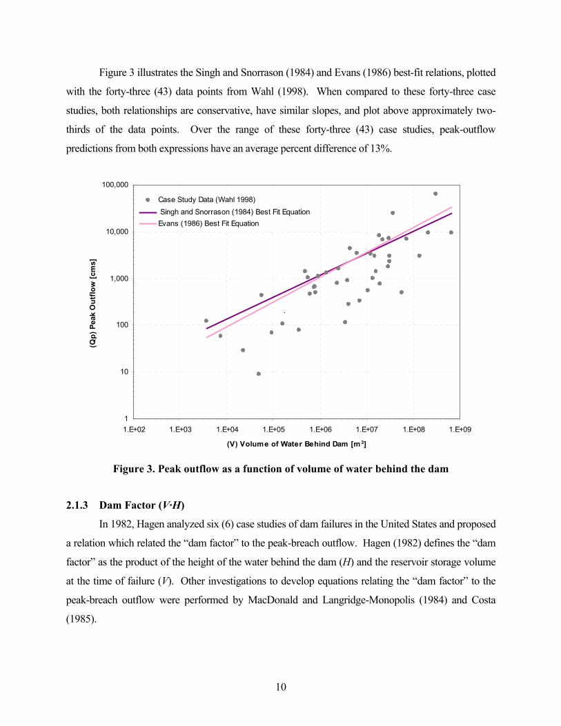
Figure 3 illustrates the Singh and Snorrason (1984) and Evans (1986) best-fit relations, plotted
with the forty-three (43) data points from Wahl (1998). When compared to these forty-three case
studies, both relationships are conservative, have similar slopes, and plot above approximately two-
thirds of the data points. Over the range of these forty-three (43) case studies, peak-outflow
predictions from both expressions have an average percent difference of 13%.
1
10
100
1,000
10,000
100,000
1.E+02 1.E+03 1.E+04 1.E+05 1.E+06 1.E+07 1.E+08 1.E+09
(V) Volume of Water Behind Dam [m3]
(Qp)
Pea
k O
utflo
w [c
ms]
Case Study Data (Wahl 1998) Singh and Snorrason (1984) Best Fit EquationEvans (1986) Best Fit Equation
.
Figure 3. Peak outflow as a function of volume of water behind the dam
2.1.3 Dam Factor (V·H)
In 1982, Hagen analyzed six (6) case studies of dam failures in the United States and proposed
a relation which related the “dam factor” to the peak-breach outflow. Hagen (1982) defines the “dam
factor” as the product of the height of the water behind the dam (H) and the reservoir storage volume
at the time of failure (V). Other investigations to develop equations relating the “dam factor” to the
peak-breach outflow were performed by MacDonald and Langridge-Monopolis (1984) and Costa
(1985).
10
MacDonald and Langridge-Monopolis (1984) analyzed forty-two (42) case studies, twenty-
three (23) of which included information regarding peak outflow. These 23 case studies were used to
develop best-fit and envelope equations for peak outflow as a function of the dam factor. Costa (1985)
analyzed thirty-one (31) dam failures and presented envelope curves and best-fit relationships based
on linear regression analysis of the case studies. The proposed best-fit relationship, presented as
Equation 10.1 (Table 1) also predicts the peak-breach discharge as a function of the dam factor.
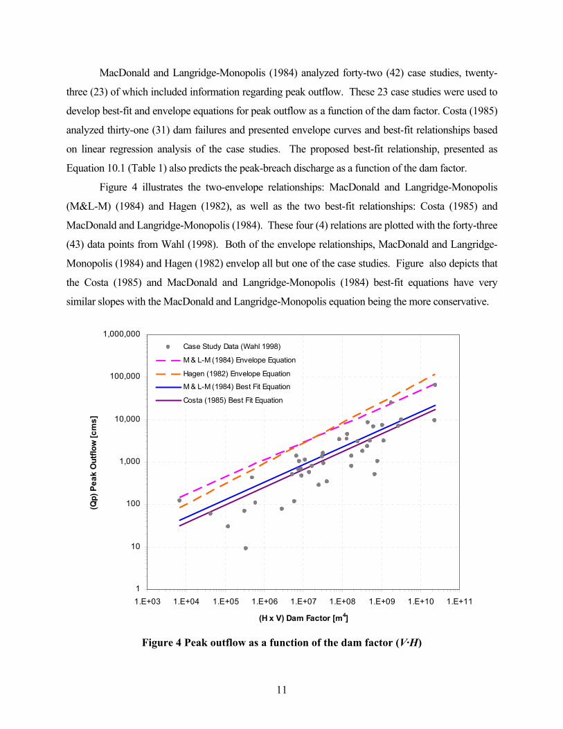
Figure 4 illustrates the two-envelope relationships: MacDonald and Langridge-Monopolis
(M&L-M) (1984) and Hagen (1982), as well as the two best-fit relationships: Costa (1985) and
MacDonald and Langridge-Monopolis (1984). These four (4) relations are plotted with the forty-three
(43) data points from Wahl (1998). Both of the envelope relationships, MacDonald and Langridge-
Monopolis (1984) and Hagen (1982) envelop all but one of the case studies. Figure also depicts that
the Costa (1985) and MacDonald and Langridge-Monopolis (1984) best-fit equations have very
similar slopes with the MacDonald and Langridge-Monopolis equation being the more conservative.
1
10
100
1,000
10,000
100,000
1,000,000
1.E+03 1.E+04 1.E+05 1.E+06 1.E+07 1.E+08 1.E+09 1.E+10 1.E+11
(H x V) Dam Factor [m4]
(Qp)
Pea
k O
utflo
w [c
ms]
Case Study Data (Wahl 1998)
M & L-M (1984) Envelope Equation
Hagen (1982) Envelope Equation
M & L-M (1984) Best Fit Equation
Costa (1985) Best Fit Equation
Figure 4 Peak outflow as a function of the dam factor (V·H)
11
2.2 Multiple-regression Analysis Froehlich (1995) introduced a best-fit relationship for predicting peak outflow as a power
function of both the volume and depth of water stored behind a dam. A series of twenty-two (22) case
studies was analyzed using multiple-regression analysis to develop Equation 11.1 presented in Table
1. Wahl (1998) used the Froehlich (1995) relationship to predict peak outflows for thirty-two (32)
case studies, including the twenty-two (22) used in the development of the equation. Based on his
analysis, Wahl (1998) suggests that the Froehlich relationship is one of the better methods for direct
prediction of peak-breach outflow.
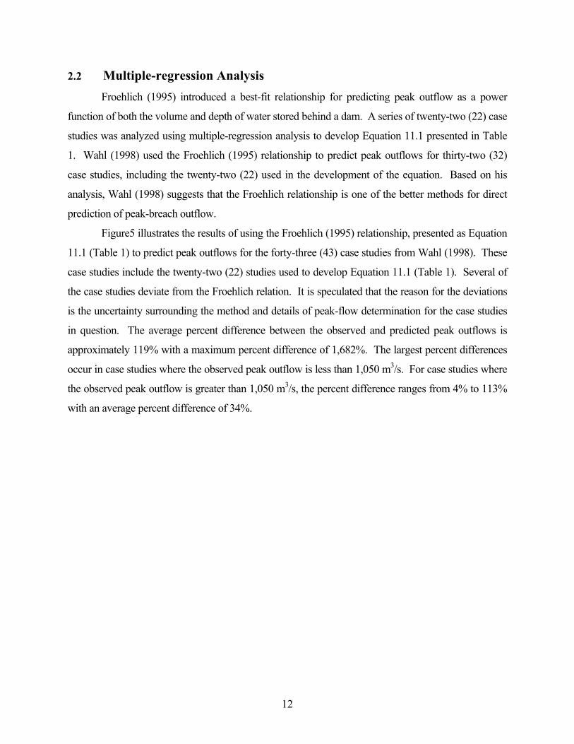
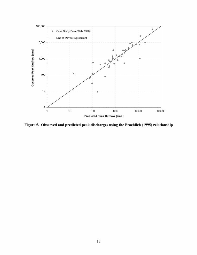
Figure5 illustrates the results of using the Froehlich (1995) relationship, presented as Equation
11.1 (Table 1) to predict peak outflows for the forty-three (43) case studies from Wahl (1998). These
case studies include the twenty-two (22) studies used to develop Equation 11.1 (Table 1). Several of
the case studies deviate from the Froehlich relation. It is speculated that the reason for the deviations
is the uncertainty surrounding the method and details of peak-flow determination for the case studies
in question. The average percent difference between the observed and predicted peak outflows is
approximately 119% with a maximum percent difference of 1,682%. The largest percent differences
occur in case studies where the observed peak outflow is less than 1,050 m3/s. For case studies where
the observed peak outflow is greater than 1,050 m3/s, the percent difference ranges from 4% to 113%
with an average percent difference of 34%.
12
1
10
100
1,000
10,000
100,000
1 10 100 1000 10000 100000
Predicted Peak Outflow [cms]
Obs
erve
d Pe
ak O
utflo
w [c
ms]
Case Study Data (Wahl 1998)
Line of Perfect Agreement
Figure 5. Observed and predicted peak discharges using the Froehlich (1995) relationship
13
14
3 EXPANDING THE DATABASE
The peak-discharge relations presented have been based on data from thirty-one (31) or fewer
case studies. Since the development of these relationships, several dams have failed providing
additional case study information. Also, large- and small-scale laboratory research has been
undertaken to improve the understanding of embankment breaching mechanisms and processes; and
provide additional data for numerical model development, calibration, and validation.
Pierce (2008) acquired dam-breach failure data from forty-four (44) case studies for breaches
occurring from 1975 through 2007. Efforts to collect this information included: (1) a survey of State
Dam Safety Officials from all fifty (50) states and Puerto Rico; (2) a review of available publications
reporting dam failures; (3) a review of published research and testing reports; and (4) a query of the
National Performance of Dams Program’s dam-failure database. A summary of these embankment-
dam failures is presented in Table 3. The additional data provide dam-failure information for dam
heights ranging from 0.60 to 31.46 m, and peak outflows ranging from 0.28 to 78,000 m3/sec.
Dam-breach data were collected (e.g., dam height, estimated peak outflow, water-storage
volume, embankment length, etc.) from 44 additional case studies. A summary of these embankment-
dam failures is presented in Table 3. The additional data provide dam-failure information for dam
heights ranging from 0.60 to 31.46 m, and peak outflows ranging from 0.28 to 78,000 m3/s.
Table 3 Case Studies Reported by Pierce (2008)
Depth of Water Behind Dam at Failure
(or Dam Height),
Volume of Water Behind
Dam at Failure
(or Storage),
Downstream Dam Slope,
Dam Width
at Crest,
Average Dam
Width, Zed Dam
Length, Peak
Outflow, Z horizontal: L QpH V Wc Wavg 1 vertical Reference Site
(m3) (m3/s) (m) (m) (m) (m) 1 Banqiao, China 26.11 6.12E+08 78000 2000.00 Fujia and Yumei (1994) 2 Big Bay Dam, MS 13.59 1.75E+07 4160 12.19 3 576.07 Burge (2004) 3 Boydstown, PA 8.96 3.58E+05 65.13 SCS (1986) 4 Caney Coon Creek, OK 4.57 1.32E+06 16.99 SCS (1986) 5 Castlewood, OK 21.34 4.23E+06 3570 SCS (1986) 6 Cherokee Sandy, OK 5.18 4.44E+05 8.5 SCS (1986) 7 Colonial #4, PA 9.91 3.82E+04 14.16 SCS (1986) 8 Dam Site #8, MS 4.57 8.70E+05 48.99 SCS (1986) 15
9 Field Test 1-1, Norway 6.1 7.30E+04 190 Hassan et al. (2004) 10 Field Test 1-2, Norway 5.9 6.30E+04 113 Hassan et al. (2004) 11 Field Test 1-3, Norway 5.9 6.30E+04 242 Vaskinn et al. (2004) 12 Field Test 2-2, Norway 5 3.59E+04 74 Hassan et al. (2004) 13 Field Test 2-3, Norway 6 6.73E+04 174 Vaskinn et al. (2004) 14 Field Test 3-3, Norway 4.3 2.20E+04 170 Vaskinn et al. (2004)
15 Haymaker, MT 4.88 3.70E+05 26.9 SCS (1986) 16 Horse Creek #2, CO 12.5 4.80E+06 311.49 SCS (1986) 17 HR Wallingford Test 10, UK 0.6 2.45E+02 0.31 Hassan et al. (2004) 18 HR Wallingford Test 11, UK 0.6 2.45E+02 0.34 Hassan et al. (2004) 19 HR Wallingford Test 12, UK 0.6 2.45E+02 0.53 Hassan et al. (2004) 20 HR Wallingford Test 14, UK 0.6 2.45E+02 0.28 Hassan et al. (2004) 21 HR Wallingford Test 15, UK 0.6 2.45E+02 0.35 Hassan et al. (2004) 22 HR Wallingford Test 16, UK 0.6 2.45E+02 0.43 Hassan et al. (2004) 23 HR Wallingford Test 17, UK 0.6 2.45E+02 0.61 Hassan et al. (2004)
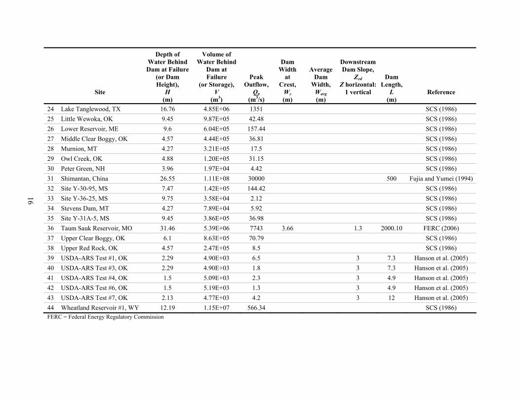
Site
Depth of Water Behind Dam at Failure
(or Dam Height),
H (m)
Volume of Water Behind
Dam at Failure
(or Storage), V
(m3)
Peak Outflow,
Qp(m3/s)
Dam Width
at Crest,
Wc(m)
Average Dam
Width, Wavg(m)
Downstream Dam Slope,
ZedZ horizontal:
1 vertical
Dam Length,
L (m)
Reference
24 Lake Tanglewood, TX 16.76 4.85E+06 1351 SCS (1986) 25 Little Wewoka, OK 9.45 9.87E+05 42.48 SCS (1986) 26 Lower Reservoir, ME 9.6 6.04E+05 157.44 SCS (1986) 27 Middle Clear Boggy, OK 4.57 4.44E+05 36.81 SCS (1986) 28 Murnion, MT 4.27 3.21E+05 17.5 SCS (1986) 29 Owl Creek, OK 4.88 1.20E+05 31.15 SCS (1986) 30 Peter Green, NH 3.96 1.97E+04 4.42 SCS (1986) 31 Shimantan, China 26.55 1.11E+08 30000 500 Fujia and Yumei (1994) 32 Site Y-30-95, MS 7.47 1.42E+05 144.42 SCS (1986) 33 Site Y-36-25, MS 9.75 3.58E+04 2.12 SCS (1986) 34 Stevens Dam, MT 4.27 7.89E+04 5.92 SCS (1986) 35 Site Y-31A-5, MS 9.45 3.86E+05 36.98 SCS (1986) 36 Taum Sauk Reservoir, MO 31.46 5.39E+06 7743 3.66 1.3 2000.10 FERC (2006) 37 Upper Clear Boggy, OK 6.1 8.63E+05 70.79 SCS (1986) 38 Upper Red Rock, OK 4.57 2.47E+05 8.5 SCS (1986) 39 USDA-ARS Test #1, OK 2.29 4.90E+03 6.5 3 7.3 Hanson et al. (2005) 40 USDA-ARS Test #3, OK 2.29 4.90E+03 1.8 3 7.3 Hanson et al. (2005) 41 USDA-ARS Test #4, OK 1.5 5.09E+03 2.3 3 4.9 Hanson et al. (2005) 42 USDA-ARS Test #6, OK 1.5 5.19E+03 1.3 3 4.9 Hanson et al. (2005) 43 USDA-ARS Test #7, OK 2.13 4.77E+03 4.2 3 12 Hanson et al. (2005)
SCS (1986) 566.34 1.15E+07 12.19
16
44 Wheatland Reservoir #1, WY FERC = Federal Energy Regulatory Commission
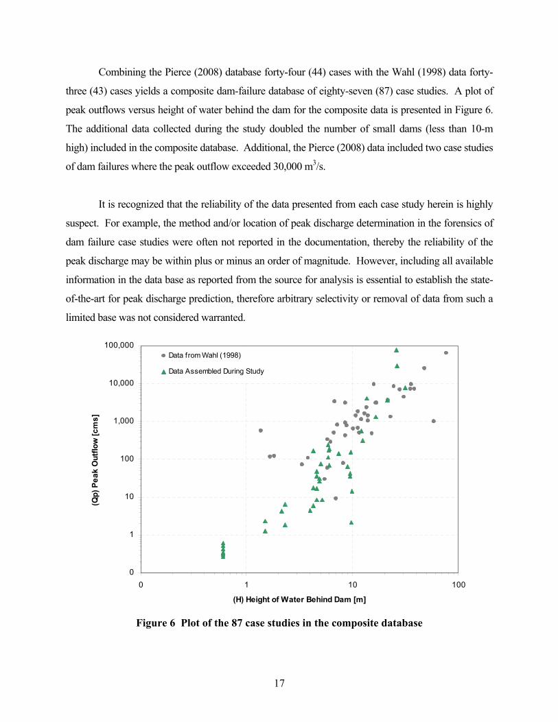
Combining the Pierce (2008) database forty-four (44) cases with the Wahl (1998) data forty-
three (43) cases yields a composite dam-failure database of eighty-seven (87) case studies. A plot of
peak outflows versus height of water behind the dam for the composite data is presented in Figure 6.
The additional data collected during the study doubled the number of small dams (less than 10-m
high) included in the composite database. Additional, the Pierce (2008) data included two case studies
of dam failures where the peak outflow exceeded 30,000 m3/s.
It is recognized that the reliability of the data presented from each case study herein is highly
suspect. For example, the method and/or location of peak discharge determination in the forensics of
dam failure case studies were often not reported in the documentation, thereby the reliability of the
peak discharge may be within plus or minus an order of magnitude. However, including all available
information in the data base as reported from the source for analysis is essential to establish the state-
of-the-art for peak discharge prediction, therefore arbitrary selectivity or removal of data from such a
limited base was not considered warranted.
0
1
10
100
1,000
10,000
100,000
0 1 10 100
(H) Height of Water Behind Dam [m]
(Qp)
Pea
k O
utflo
w [c
ms]
Data from Wahl (1998)
Data Assembled During Study
Figure 6 Plot of the 87 case studies in the composite database
17
4 ANALYSIS OF H, V, W AND L TERMS
A series of regression analyses was performed using the composite database. A summary of
this analysis is presented. Two terms were used to represent the effective head and storage
parameters. The term “H” represents the height of the water behind the dam at failure and was used to
combine the hw and hd terms previously presented. In all case studies where the height of the water
behind the dam at failure (hw) was reported, H was used in the place of hw. If the hw term was not
reported, and the dam failed by overtopping, the height of the dam (hd) was used as a substitute for hw.
If the dam failed by means other than overtopping and the hw term was not reported, the case study
was not used. The term “V” represents the volume of water behind the dam at failure and was used to
combine the terms Vw and S. If a value of Vw was reported, V was used in place of Vw. If the Vw term
was not reported, S was assumed to be an approximation of Vw.
The Pierce et al. (2010) database contained thirty-eight (38) studies that reported dam length
(L), average dam width (Wave), or both length and width information (25 studies reporting average
dam width, 14 studies reporting dam length, and 4 studies with both dam length and average width. A
series of regression analyses will be performed to correlate these terms to peak discharge as
embankment failure as well.
4.1 Linear Regression (Qp and H) Observation of the data presented in Figure 5 indicates that a relationship exists between the
height of the water behind the dam (H) and peak outflow (Qp). However, it is apparent that when H is
less than 3 m, the data does not fit the trend of dams of greater height. Therefore, the analysis of Qp as
a function of H focused exclusively on the seventy-two (72) casse studies where H was greater than 3
m. Linear-regression analysis was performed on the logarithmic transformation of the composite data
to develop a best-fit expression for predicting peak outflow from a breached embankment dam. The
best-fit relation is expressed by Equation 1 and illustrated in Figure 7. The coefficient of
determination (R2) of Equation 1 is 0.675. When compared to the R2 values of the previous
relationships listed in Table 1, Equation 1 ranks in the lower 30%. However, Equation 1 was
developed from an expanded database with considerable scatter:
18
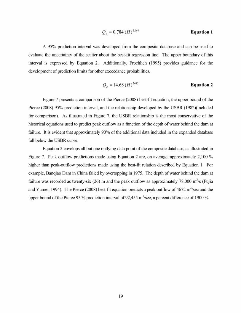
Equation 1 668.2)(784.0 HQp =
A 95% prediction interval was developed from the composite database and can be used to
evaluate the uncertainty of the scatter about the best-fit regression line. The upper boundary of this
interval is expressed by Equation 2. Additionally, Froehlich (1995) provides guidance for the
development of prediction limits for other exceedance probabilities.
6852)(68.14 HQp = Equation 2
Figure 7 presents a comparison of the Pierce (2008) best-fit equation, the upper bound of the
Pierce (2008) 95% prediction interval, and the relationship developed by the USBR (1982)(included
for comparison). As illustrated in Figure 7, the USBR relationship is the most conservative of the
historical equations used to predict peak outflow as a function of the depth of water behind the dam at
failure. It is evident that approximately 90% of the additional data included in the expanded database
fall below the USBR curve.
Equation 2 envelops all but one outlying data point of the composite database, as illustrated in
Figure 7. Peak outflow predictions made using Equation 2 are, on average, approximately 2,100 %
higher than peak-outflow predictions made using the best-fit relation described by Equation 1. For
example, Banqiao Dam in China failed by overtopping in 1975. The depth of water behind the dam at
failure was recorded as twenty-six (26) m and the peak outflow as approximately 78,000 m3/s (Fujia
and Yumei, 1994). The Pierce (2008) best-fit equation predicts a peak outflow of 4672 m3/sec and the
upper bound of the Pierce 95 % prediction interval of 92,455 m3/sec, a percent difference of 1900 %.
19
1
10
100
1,000
10,000
100,000
1,000,000
10,000,000
1 10
(H) Height of Water Behind Dam [m]
(Qp)
Pea
k O
utflo
w [c
ms]
100
Composite Database
Upper Bound 95% Prediction Interval (Qp, H)
Reclamation (1982) Envelope Equation
Linear Best-fit Equation (Qp, H)
Figure 7 Comparison of the Equation 2 95% prediction interval, Equation 1 best-fit, and
USBR (1982) envelope relationships
The addition of the expanded Pierce database (primarily smaller dams) to the regression
analysis has significantly increased the slope and decreased the y-intercept of the best-fit relation
(Equation 1) when compared to the USBR (1982) envelope equation. Near a dam height of 3 m, the
95% prediction interval and the USBR equation provide similar estimates of peak outflow, but diverge
as dam height increases. Equation 1 and the USBR (1982) equation converge at a dam height of
approximately 50 m.
4.2 Curvilinear Regression (Qp and H)
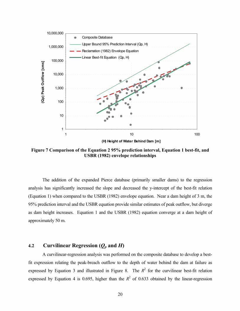
A curvilinear-regression analysis was performed on the composite database to develop a best-
fit expression relating the peak-breach outflow to the depth of water behind the dam at failure as
expressed by Equation 3 and illustrated in Figure 8. The R2 for the curvilinear best-fit relation
expressed by Equation 4 is 0.695, higher than the R2 of 0.633 obtained by the linear-regression
20
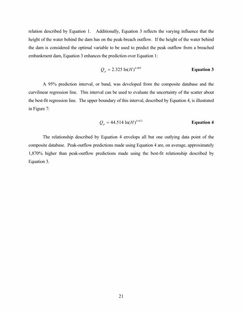
relation described by Equation 1. Additionally, Equation 3 reflects the varying influence that the
height of the water behind the dam has on the peak-breach outflow. If the height of the water behind
the dam is considered the optimal variable to be used to predict the peak outflow from a breached
embankment dam, Equation 3 enhances the prediction over Equation 1:
405.6)ln(325.2 HQp = Equation 3
A 95% prediction interval, or band, was developed from the composite database and the
curvilinear regression line. This interval can be used to evaluate the uncertainty of the scatter about
the best-fit regression line. The upper boundary of this interval, described by Equation 4, is illustrated
in Figure 7:
412.6)ln(514.44 HQp = Equation 4
The relationship described by Equation 4 envelops all but one outlying data point of the
composite database. Peak-outflow predictions made using Equation 4 are, on average, approximately
1,870% higher than peak-outflow predictions made using the best-fit relationship described by
Equation 3.
21
1
10
100
1,000
10,000
100,000
1,000,000
1 10 100
(H) Height of Water Behind Dam [m]
(Qp)
Pea
k O
utflo
w [c
ms]
Composite DatabaseUpper Bound 95% Prediction Interval (Qp, H)Curvilinear Best-f it Equation (Qp, H)
Figure 7 Curvilinear-regression analysis of the composite database (Qp and H)
4.3 Linear Regression (Qp and V) The volume of water behind the dam was analyzed as a predictor variable for peak-breach
discharge. A linear-regression analysis was performed to determine a best-fit expression predicting
peak outflow from a breached embankment dam as a function of the volume of water behind the dam.
The resulting relation is described by Equation 5 and illustrated in Figure 9. The R2 of Equation 5 is
0.805. When compared to the R2 values of the previous relations listed in Table 1, Equation 5 ranks in
the top 40%:
745.0)(00919.0 VQp = Equation 5
22
0
1
10
100
1,000
10,000
100,000
1.E+00 1.E+01 1.E+02 1.E+03 1.E+04 1.E+05 1.E+06 1.E+07 1.E+08 1.E+09
(V) Volume of Water Behind Dam [m 3]
(Qp)
Pea
k O
utflo
w [c
ms]
Composite Database
Singh and Snorrason (1984) Best-Fit Equation
Evans (1986) Best-Fit Equation Linear Best-Fit Equation (Qp, V)
Figure 9 Comparison of the Singh and Snorrason (1984), Evans (1986), and Equation 5
linear best-fit equations
Figure 8 compares the Pierce (2008) best-fit relation developed from the regression analysis of
the composite database to the Evans (1986) and Singh and Snorrason (1984) relationships. The
inclusion of a larger number of low-volume reservoirs in the composite database resulted in a best-fit
relation with a greater slope than historical equations. It appears that relatively small changes in the
volume of water behind the dam have a greater influence on the predicted peak outflow than
previously believed.
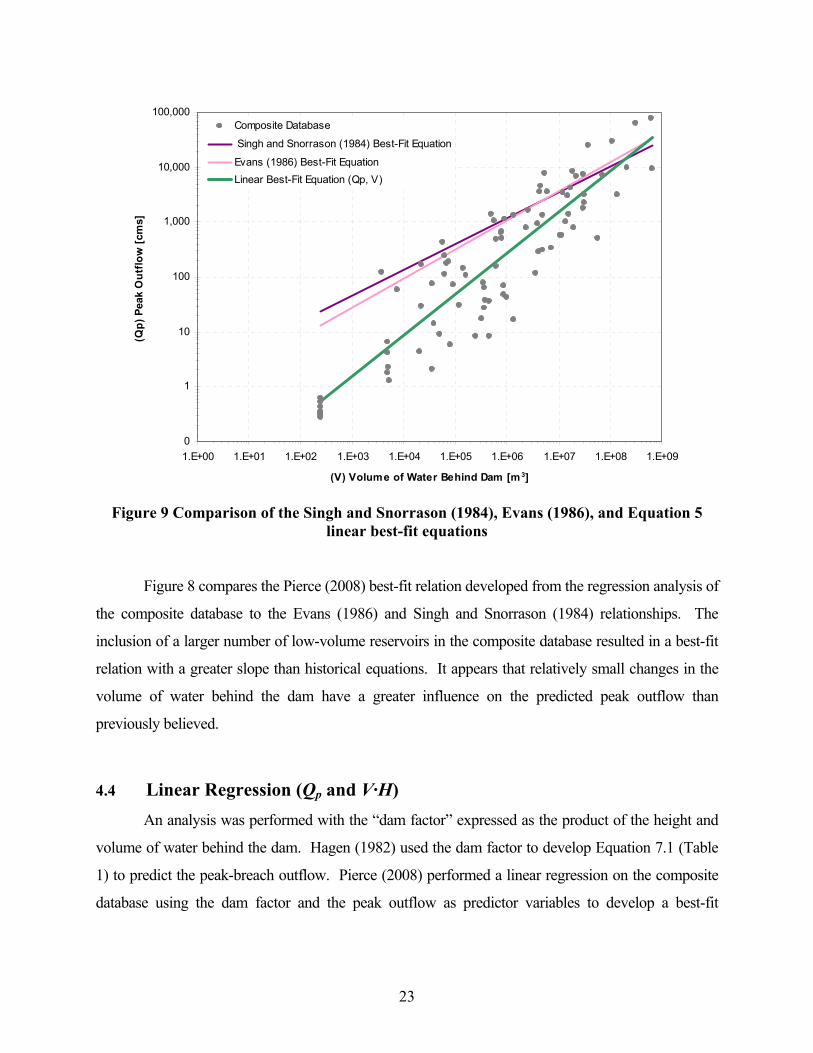
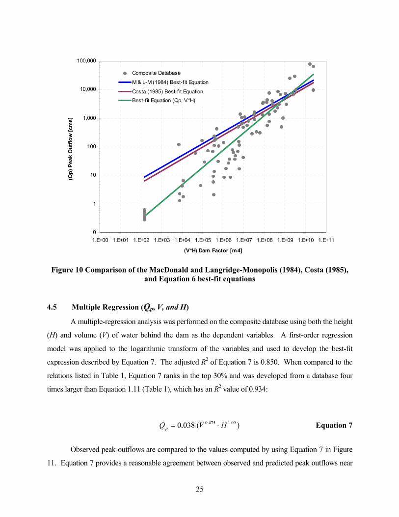
4.4 Linear Regression (Qp and V·H) An analysis was performed with the “dam factor” expressed as the product of the height and
volume of water behind the dam. Hagen (1982) used the dam factor to develop Equation 7.1 (Table
1) to predict the peak-breach outflow. Pierce (2008) performed a linear regression on the composite
database using the dam factor and the peak outflow as predictor variables to develop a best-fit
23
predictive expression. The resulting relationship is expressed by Equation 6 and illustrated in Figure
10:
606.0)(0176.0 HVQp ⋅= Equation 6
The R2 of Equation 6 is 0.844. When compared to the R2 values of the previous relations
listed in Table 1, Equation 6 ranks in the top 30% of all the predictive relationships. Equation 6 has a
greater R2 than other relations which use the dam factor as the dependent variable. Further, Equation
6 was developed from a database of eighty-seven (87) case studies compared to twenty-three (23) and
thirty-one (31) case studies for the MacDonald and Langridge-Monopolis (1984) and Costa (1985)
relationships, respectively.
Figure 10 presents a comparison of best-fit relations predicting peak outflow as a function of
the dam factor, the Costa (1985), MacDonald and Langridge-Monopolis (1984), and Pierce (2008)
equations. It is observed that the MacDonald and Langridge-Monopolis relationship is the more
conservative of the historical equations used to predict peak outflow as a function of the dam factor. It
is evident that most of the case studies with a dam factor of between 100 and 10,000,000 (m4) plot
below the MacDonald and Langridge-Monopolis curve. Thus, the best-fit relation expressed by
Equation 6 has a smaller y-intercept and a steeper slope. The average percent difference between
Equation 6 and the MacDonald and Langridge-Monopolis best-fit equation between 100 and
10,000,000 (m4) is approximately 650%, while above 10,000,000 (m4) the average percent difference
reduces to approximately 40%.
24
0
1
10
100
1,000
10,000
100,000
1.E+00 1.E+01 1.E+02 1.E+03 1.E+04 1.E+05 1.E+06 1.E+07 1.E+08 1.E+09 1.E+10 1.E+11
(V*H) Dam Factor [m4]
(Qp)
Pea
k O
utflo
w [c
ms]
Composite Database
M & L-M (1984) Best-f it Equation
Costa (1985) Best-f it EquationBest-f it Equation (Qp, V*H)
Figure 10 Comparison of the MacDonald and Langridge-Monopolis (1984), Costa (1985),
and Equation 6 best-fit equations
4.5 Multiple Regression (Qp, V, and H)
A multiple-regression analysis was performed on the composite database using both the height
(H) and volume (V) of water behind the dam as the dependent variables. A first-order regression
model was applied to the logarithmic transform of the variables and used to develop the best-fit
expression described by Equation 7. The adjusted R2 of Equation 7 is 0.850. When compared to the
relations listed in Table 1, Equation 7 ranks in the top 30% and was developed from a database four
times larger than Equation 1.11 (Table 1), which has an R2 value of 0.934:
)(038.0 09.1475.0 HVQp ⋅= Equation 7
Observed peak outflows are compared to the values computed by using Equation 7 in Figure
11. Equation 7 provides a reasonable agreement between observed and predicted peak outflows near
25
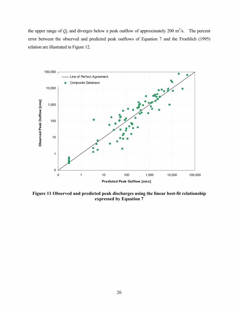
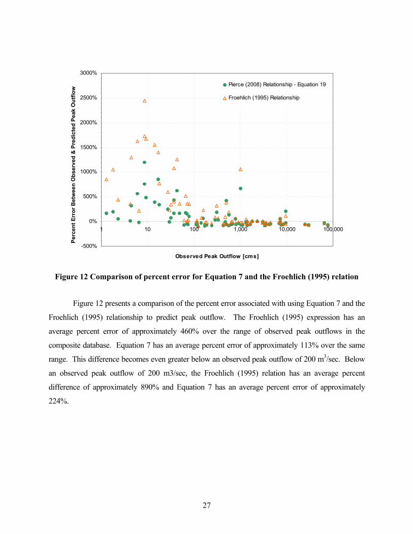
the upper range of Qp and diverges below a peak outflow of approximately 200 m3/s. The percent
error between the observed and predicted peak outflows of Equation 7 and the Froehlich (1995)
relation are illustrated in Figure 12.
0
1
10
100
1,000
10,000
100,000
0 1 10 100 1,000 10,000 100,000
Predicted Peak Outflow [cms]
Obs
erve
d Pe
ak O
utflo
w [c
ms]
Line of Perfect Agreement
Composite Database
Figure 11 Observed and predicted peak discharges using the linear best-fit relationship
expressed by Equation 7
26
-500%
0%
500%
1000%
1500%
2000%
2500%
3000%
1 10 100 1,000 10,000 100,000
Observed Peak Outflow [cms]
Perc
ent E
rror
Bet
wee
n O
bser
ved
& P
redi
cted
Pea
k O
utflo
w Pierce (2008) Relationship - Equation 19
Froehlich (1995) Relationship
Figure 12 Comparison of percent error for Equation 7 and the Froehlich (1995) relation
Figure 12 presents a comparison of the percent error associated with using Equation 7 and the
Froehlich (1995) relationship to predict peak outflow. The Froehlich (1995) expression has an
average percent error of approximately 460% over the range of observed peak outflows in the
composite database. Equation 7 has an average percent error of approximately 113% over the same
range. This difference becomes even greater below an observed peak outflow of 200 m3/sec. Below
an observed peak outflow of 200 m3/sec, the Froehlich (1995) relation has an average percent
difference of approximately 890% and Equation 7 has an average percent error of approximately
224%.
27
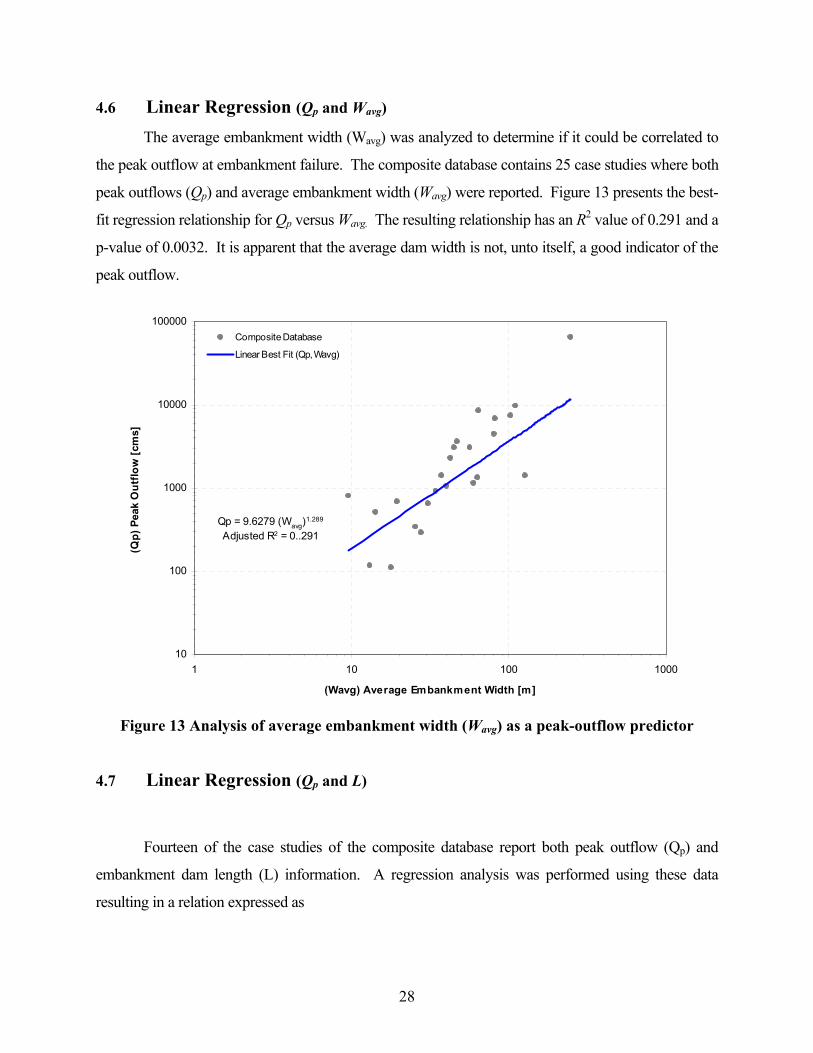
4.6 Linear Regression (Qp and Wavg) The average embankment width (Wavg) was analyzed to determine if it could be correlated to
the peak outflow at embankment failure. The composite database contains 25 case studies where both
peak outflows (Qp) and average embankment width (Wavg) were reported. Figure 13 presents the best-
fit regression relationship for Qp versus Wavg. The resulting relationship has an R2 value of 0.291 and a
p-value of 0.0032. It is apparent that the average dam width is not, unto itself, a good indicator of the
peak outflow.
Qp = 9.6279 (Wavg)1.289
Adjusted R2 = 0..291
10
100
1000
10000
100000
1 10 100 1000
(Wavg) Average Embankment Width [m]
(Qp)
Pea
k O
utflo
w [c
ms]
Composite Database
Linear Best Fit (Qp, Wavg)
Figure 13 Analysis of average embankment width (Wavg) as a peak-outflow predictor
4.7 Linear Regression (Qp and L)
Fourteen of the case studies of the composite database report both peak outflow (Qp) and
embankment dam length (L) information. A regression analysis was performed using these data
resulting in a relation expressed as
28
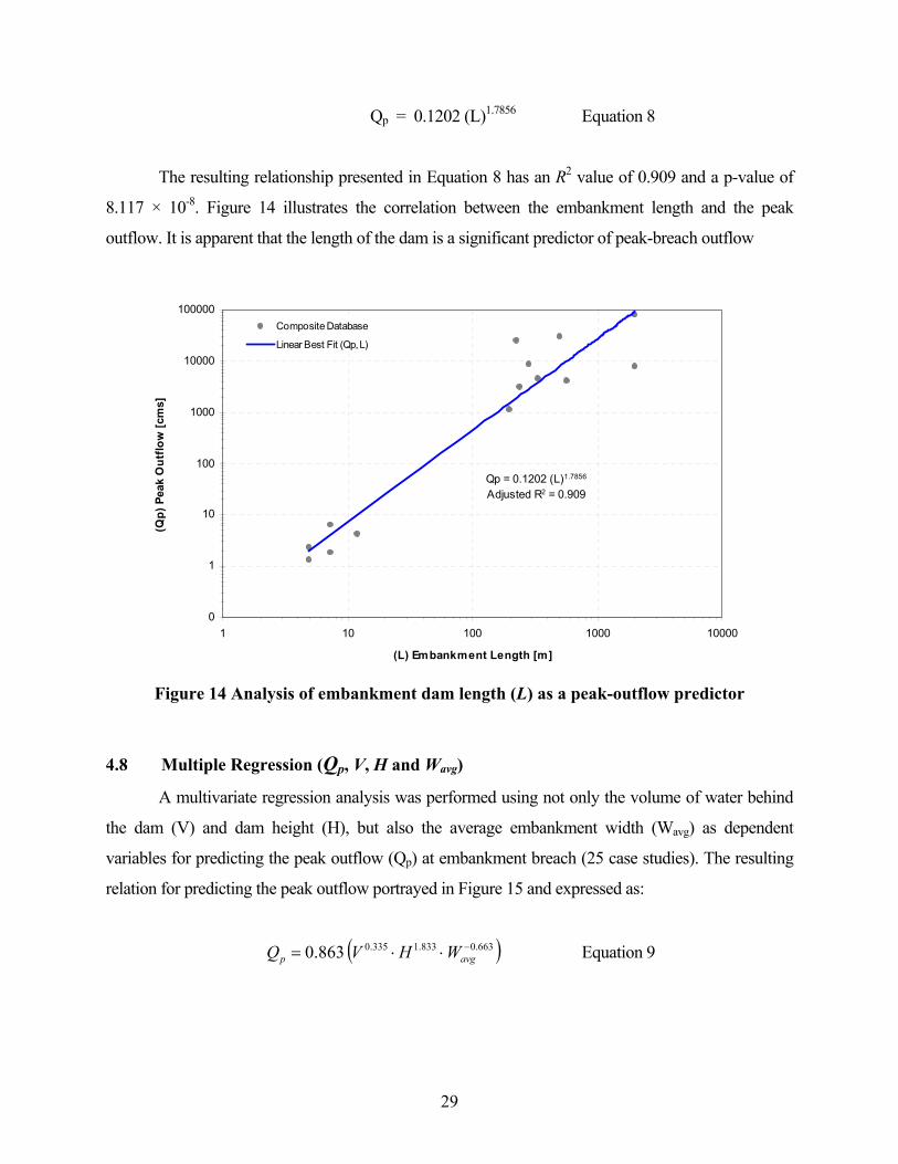
Qp = 0.1202 (L)1.7856 Equation 8
The resulting relationship presented in Equation 8 has an R2 value of 0.909 and a p-value of
8.117 × 10⁻⁸. Figure 14 illustrates the correlation between the embankment length and the peak
outflow. It is apparent that the length of the dam is a significant predictor of peak-breach outflow
Qp = 0.1202 (L)1.7856
Adjusted R2 = 0.909
0
1
10
100
1000
10000
100000
1 10 100 1000 10000
(L) Embankment Length [m]
(Qp)
Pea
k O
utflo
w [c
ms]
Composite Database
Linear Best Fit (Qp, L)
Figure 14 Analysis of embankment dam length (L) as a peak-outflow predictor
4.8 Multiple Regression (Qp, V, H and Wavg)
A multivariate regression analysis was performed using not only the volume of water behind
the dam (V) and dam height (H), but also the average embankment width (Wavg) as dependent
variables for predicting the peak outflow (Qp) at embankment breach (25 case studies). The resulting
relation for predicting the peak outflow portrayed in Figure 15 and expressed as:
( )663.0833.1335.0863.0 −⋅⋅= avgp WHVQ Equation 9
29
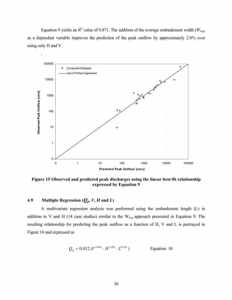
Equation 9 yields an R2 value of 0.871. The addition of the average embankment width (Wavg)
as a dependant variable improves the prediction of the peak outflow by approximately 2.8% over
using only H and V.
.
0
1
10
100
1000
10000
100000
0 1 10 100 1000 10000 100000
Predicted Peak Outflow [cms]
Obs
erve
d Pe
ak O
utflo
w [c
ms]
Composite Database
Line of Perfect Agreement
Figure 15 Observed and predicted peak discharges using the linear best-fit relationship
expressed by Equation 9
4.9 Multiple Regression (Qp, V, H and L)
A multivariate regression analysis was performed using the embankment length (L) in
addition to V and H (14 case studies) similar to the Wavg approach presented in Equation 9. The
resulting relationship for predicting the peak outflow as a function of H, V and L is portrayed in
Figure 16 and expressed as
)(012.0 226.0205.1493.0 LHVQp ⋅⋅= Equation 10
30
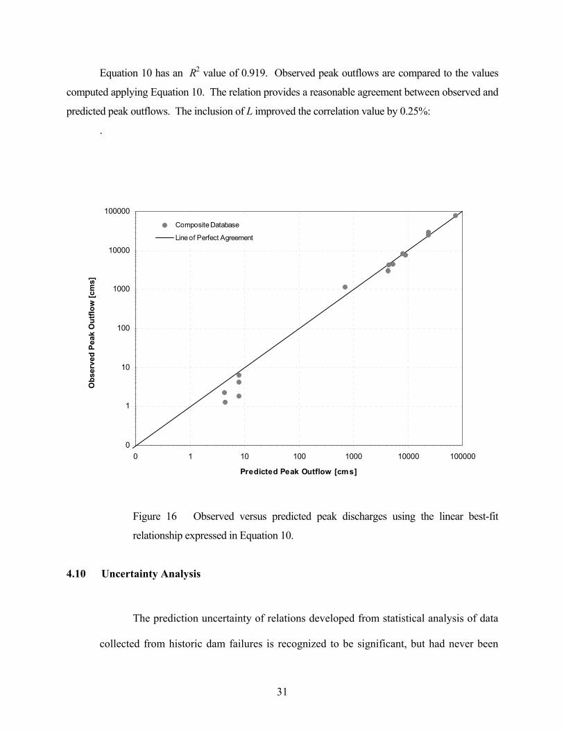
Equation 10 has an R2 value of 0.919. Observed peak outflows are compared to the values
computed applying Equation 10. The relation provides a reasonable agreement between observed and
predicted peak outflows. The inclusion of L improved the correlation value by 0.25%:
.
0
1
10
100
1000
10000
100000
0 1 10 100 1000 10000 100000
Predicted Peak Outflow [cms]
Obs
erve
d Pe
ak O
utflo
w [c
ms]
Composite Database
Line of Perfect Agreement
Figure 16 Observed versus predicted peak discharges using the linear best-fit
relationship expressed in Equation 10.
4.10 Uncertainty Analysis
The prediction uncertainty of relations developed from statistical analysis of data
collected from historic dam failures is recognized to be significant, but had never been
31
specifically quantified until Wahl (2004). Wahl (2004) presents a description of the
uncertainty analysis method used as well as a comparison of uncertainty estimates for H,
V, H, V.H and (V and H) breach parameter and peak outflow prediction equations. The
methods used by Wahl were applied to the Pierce (2008) equations. Table 4 presents the
results of this analysis as well as a summary of the Wahl (2004) analysis.
It is observed that the Pierce relationships tend to under predict observed peak
flows. On average, Equation 3 best predicts the peak outflow under estimating by only -
0.058 log cycles while Equation 1 under predicts the peak outflow the most at -0.037 log
cycles. The uncertainty bands for all of the presented peak outflow prediction equations
range from +0.3 to +0.9 of an order of magnitude. The uncertainty bands for the Pierce
equations were consistently between +0.45 and +0.60 of an order of magnitude.
Equation 5 has both the lowest prediction error and the smallest uncertainty for the
volume of water relations. Equation 6 has both the lowest prediction error and the
smallest uncertainty for the dam factor relations. Equations 3-7 have mean prediction
errors of 0.006 an order of magnitude or less.
An uncertainty analysis was also performed on the parameters of H, V and Wavg
as well as H, V and L versus Qp as portrayed in Table 4. It is observed that the prediction
error of the relations derived from the single variable (i.e. H, V or V.H) tend to be an
order of magnitude or more, greater than the relations with multiple variables (i.e. V and
H; V, H and L, etc.) with the exception of the Pierce (2008) expressions. Further, peak
flow prediction equations using the three variables show a slight reduction in mean
predictions error (-0.005 to -0.011) over the two variable peak flow equations (-0.010 to -
0.04).
32
Insert Table 4
A comparison of the percent error between observed and predicted peak outflows
was performed for the Froehlich (1995) relation and Equation 10 as illustrated in Figure
16. It is apparent that for discharges above 1,000 cms, the Froehlich and Equation 10
relations provide similar variance, although the Froehlich relation displays a slightly
higher deviation. The Froehlich relation was not developed for low flows.
The trends depicted in the prediction error analysis closely align with the
comparison of band width uncertainty analyses shown in Table 4. The band width for
peak flow prediction expressions using the single dependent variable ranges from
approximately +0.45 to +0.93, or nearly an order of magnitude variance. The band width
for the peak flow prediction using two variables reduces the variance to approximately
+0.32 to +0.75, or approximately ¾ an order of magnitude. The three variable peak flow
prediction relations reduce the band width uncertainty even further to +0.15 to +0.16. As
the number of significant embankment characteristics increases, the band width
uncertainty decreases using the case studies presented in Table 4.
A comparison of four (4) dam breach peak flow (Qp) prediction procedures was
performed to sensitize the user as to the broad range of estimates that may result applying
a regression approach. From the thirty-eight (38) case studies that report forensic values
for H, V, Wavg, L and Qp; they include Baldwin Hills, CA., Hatchtown, UT, Johnstown,
PA., and Schaeffer, CO. Two peak flow predictions procedures used were those
recommended by Pierce (2008)(Eqn. 6); the H.V expressions derived by Froehlich
33
(1995)(Eqn. 11.1) and Pierce as presented in Table 5. The remaining two procedures
applied in the comparison are Equation 9 (V, H and Wavg) and Equation 10 (V, H and
L).
Insert Table 5
The case study characteristic values from Table 5 were inserted into the four (4)
predictions procedures yielding the peak flows presented in Table XXX to include the
reported Qp from the dam failure forensics. It is observed that the Pierce (2008) (Eqn. 6)
expression consistently underestimates the reported Qp values by a factor of
approximately 1.5 to 3. The low prediction estimates are attributed to the influence of the
large number of small dams included in the composite data base. The Froehlich
(1995)(Eqn. 11.1) expression also under predicts the reported Qp values, but with a
slightly improved factor of variance of approximately 1.25 to 2. Equations 9 and 10
provide similar prediction variances with predicted versus reported Qp values differing by
a factor of approximately 1.0 to 1.6. Further, it observed that Equations 9 and 10 Qp
predictions bound both above and below the reported Qp from the case studies.
It is recognized that the four (4) case studies used for this comparison do not fully
represent the spectrum of dam failures that have been recorded and therefore, the results
presented in Table 5 are biased due to the incompleteness of the database. Further,
Equations 9 and 10 are derived from small data pools. However, the comparison does
indicate that Equations 9 and 10 portray a trend of improvement using multiple variables
in performing the regression analysis, particularly as the characteristic values of the data
pool expand.
34
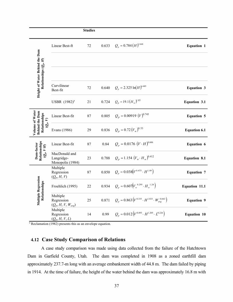
4.11 COMPARISON OF RELATIONSHIPS
A comparison of selected historical and composite-data (Pierce 2008) best-fit expressions is
depicted in Table 6. The historical relations in this comparison were selected for their high correlation
values and non-simulated case studies. The relations are segmented into groups according to the
dependent variable(s) used in the regression analysis. The number of case studies used to develop the
relations is also presented.
Five relationships predicting peak outflow as a function of the height of the water behind the
dam are presented in Table 5. The linear relationships, USBR (1982) expressed by Equation 3.1
(Table 1) and Pierce (2008) expressed by Equation 1 in Table 5, have similar R2 values, 0.633 and
0.724, respectively. However, the addition of the Pierce (2008) data, primarily smaller dams, to the
regression database has significantly increased the slope and decreased the y-intercept of Equation 1
when compared to the USBR (1982) envelope relationship. Figure 6 illustrates that for smaller dams,
the USBR (1982) relationship is more conservative than Equation 1, although the equations converge
at a dam height of approximately 50 m.
The curvilinear relation reflects the greater impact that the height of the dam has on the breach
outflow for dams less than 6.5-m high, and has an R2 value comparable to the USBR (1982) relation
(0.640 and 0.724, respectively). Additionally, Equation 3 was developed from a database of seventy-
seven (77) case studies compared to twenty-one (21) case studies for the USBR (1982) relation.
The Evans (1986) relationship expressed by Equation 6.1 (Table 1) and the Pierce (2008)
relation (Equation 5) represent equations predicting peak outflow as a function of the volume of water
behind the dam. Figure 9 illustrates that the Evans (1986) best-fit expression plots above
approximately 80% of the data contained in the composite database and provides a more conservative
estimate of peak outflow than Equation 5. Both relations have comparable R2 values (0.836 and 0.805,
respectively) although when plotted with the Pierce (2008) database, the Evans (1986) equation
appears to be more of an enveloping relation, while Equation 5 provides a best-fit estimate of peak
outflow.
The MacDonald and Langridge-Monopolis (1984) relationship expressed by Equation 8.1
(Table 1) and Pierce (2008) expressed by Equation 6 depict similar relations predicting peak-breach
outflow as a function of the dam factor. Equation 6 has an R2 value of 0.844 and the MacDonald and
Langridge-Monopolis (1984) equation has an R2 value of 0.788. In addition to an enhanced
correlation, Equation 6 was developed from a database of eighty-seven (87) case studies, over three
35

times larger than the database of twenty-three (23) case studies used to develop the MacDonald and
Langridge-Monopolis (1984) relationship. Equation 6 appears to provide an improved means of
predicting peak discharge using the dam factor as the dependent parameter.
Froehlich (1995) demonstrated that a multiple-regression relationship using both the height
and volume of water behind the dam as regression variables can be used to predict peak outflow with
reliable results. The Pierce (2008) multiple-regression relation (Equation 7) with a corresponding R2
value of 0.850 appears to be an improved peak-discharge predictor over the Froehlich (1995) relation
as Froehlich (1995) has an average percent error of approximately 460% and Equation 7 has an
average percent error of approximately 113%. Below discharges of 200 m3/s, both the Froehlich
(1995) expression and Equation 7 tend to over predict peak outflows.
It is observed that the relationships developed using H as the dependent variable result in
moderate correlations ranging from approximately 0.40 to 0.79. Although the height of water behind
the dam (H) is the easier parameter to measure in the field, the scatter of data is significant and
predictive qualities moderate. Relationships derived from case studies using the volume of water
behind the dam (V) as the dependent variable display an improvement in correlation over relations
using the height of the water behind the dam (H), values ranging from 0.81 to 0.84. When multiple
variables are used (i.e., dam factor or multivariable), correlation values again increase ranging from
0.76 to 0.93. Based upon the analyses presented herein, the dam factor and multivariable regression
approaches provide better predictive resolution than do the linear or curvilinear approaches using a
single parameter, dependent variable approach. It is recognized that the composite database represents
but a fraction of the number of embankment failures of record. However, until dam owners and
responsible agencies improve their forensic approaches to data collection after failure, the composite
database is the most comprehensive information available.
Table 6 Comparison of predictive relationships
Number of Case R2Investigator Equation and No.
36
Studies
( ) 668.2784.0 HQp = Equation 1 Linear Best-ft 72 0.633
Hei
ght o
f Wat
er B
ehin
d th
e D
am
Rel
atio
nshi
ps (Q
p, H
)
Curvilinear Best-fit 72 0.640 ( ) 405.6ln325.2 HQp = Equation 3
USBR (1982)a 21 0.724 ( ) 85.11.19 wp HQ = Equation 3.1
Vol
ume
of W
ater
B
ehin
d th
e D
am
Rel
atio
nshi
ps
(Qp,
V) ( ) 745.0 00919.0 VQp = Equation 5 Linear Best-fit 87 0.805
( ) 53.072.0 wp VQ = Equation 6.1 Evans (1986) 29 0.836
Dam
-fac
tor
Rel
atio
nshi
ps
(Qp,
V·H
) ( ) 606.0 0176.0 HVQp ⋅= Equation 6 Linear Best-fit 87 0.84
MacDonald and Langridge-Monopolis (1984)
23 0.788 ( ) 412.0 154.1 wwp HVQ ⋅= Equation 8.1
Multiple Regression (Qp, H, V)
87 0.850 ( )09.1475.0038.0 HVQp ⋅= Equation 7
Mul
tiple
Reg
ress
ion
Rel
atio
nshi
ps
( )24.1295.0607.0 wwp HVQ ⋅= Equation 11.1 Froehlich (1995) 22 0.934
Multiple Regression (Qp, H, V, Wavg)
25 0.871 ( )663.0833.1335.0863.0 −⋅⋅= avgp WHVQ Equation 9
Multiple Regression (Qp, H, V, L)
14 0.99 ( )226.0205.1493.0012.0 LHVQp ⋅⋅= Equation 10
a Reclamation (1982) presents this as an envelope equation.
4.12 Case Study Comparison of Relations A case study comparison was made using data collected from the failure of the Hatchtown
Dam in Garfield County, Utah. The dam was completed in 1908 as a zoned earthfill dam
approximately 237.7-m long with an average embankment width of 44.8 m. The dam failed by piping
in 1914. At the time of failure, the height of the water behind the dam was approximately 16.8 m with
37

a reservoir volume of approximately 1.48 × 10⁷ m3. The peak outflow through the dam breach was
calculated to be 3,080 m3/s. The peak outflow through the dam breach was predicted using selected
relationships from Table 7. These relations are presented with the variables used, the predicted peak
outflow, and the percent error of the predicted value.
38
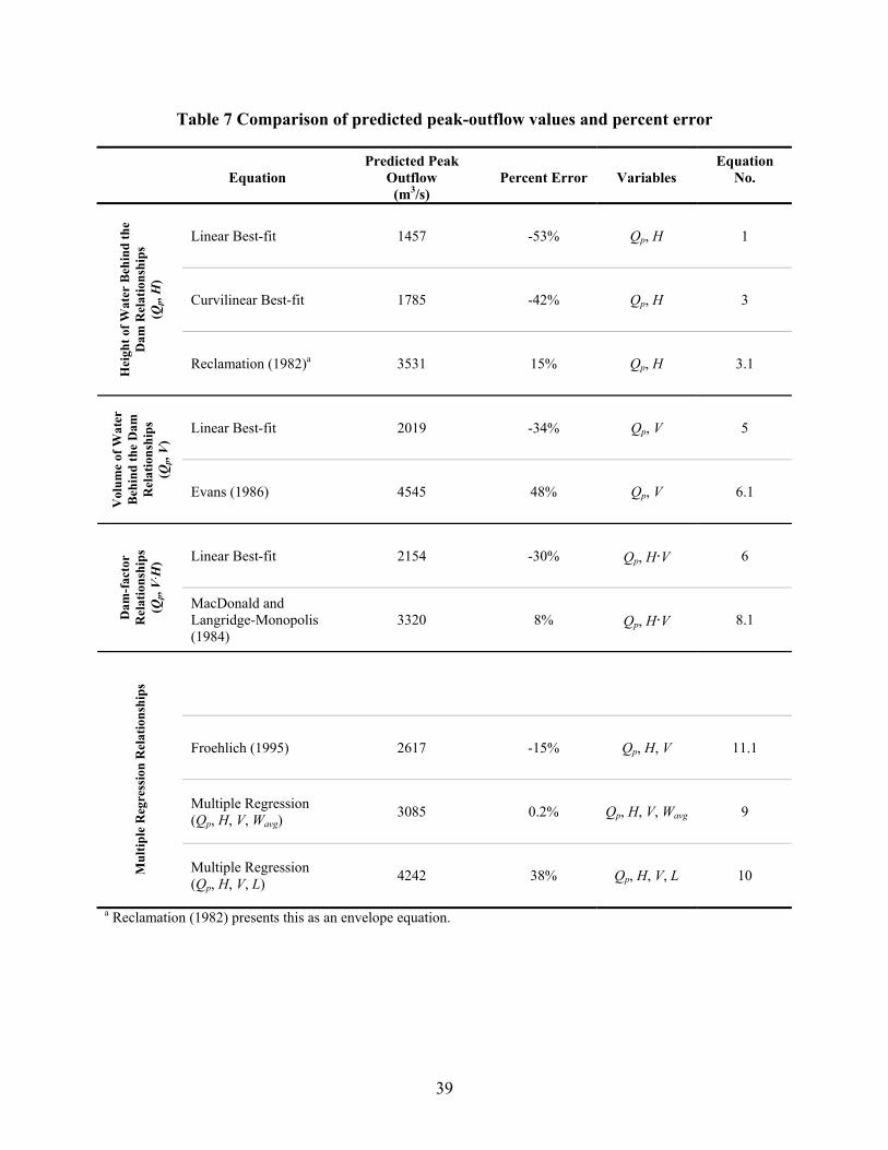
Table 7 Comparison of predicted peak-outflow values and percent error
Predicted Peak Outflow
Equation No. Equation Percent Error Variables
(m3/s)
Hei
ght o
f Wat
er B
ehin
d th
e D
am R
elat
ions
hips
(Q
p, H
)
Qp, H Linear Best-fit 1457 -53% 1
Qp, H Curvilinear Best-fit 1785 -42% 3
Reclamation (1982)a 3531 15% Qp, H 3.1
Vol
ume
of W
ater
B
ehin
d th
e D
am
Rel
atio
nshi
ps
(Qp,
V)
Qp, V Linear Best-fit 2019 -34% 5
Qp, V Evans (1986) 4545 48% 6.1
Dam
-fac
tor
Rel
atio
nshi
ps
(Qp,
V·H
) Qp, H·V 6 Linear Best-fit 2154 -30%
MacDonald and Langridge-Monopolis (1984)
3320 8% Qp, H·V 8.1
Mul
tiple
Reg
ress
ion
Rel
atio
nshi
ps
Qp, H, V Froehlich (1995) 2617 -15% 11.1
Multiple Regression (Qp, H, V, Wavg)
3085 0.2% Qp, H, V, Wavg 9
Multiple Regression (Qp, H, V, L) 4242 38% Qp, H, V, L 10
a Reclamation (1982) presents this as an envelope equation.
39
Percent error for the relationships using the height of water behind the dam as the primary predictor
variable demonstrate a percent error ranging from 15% to -53%. Of the newly-developed relations,
the curvilinear best-fit relationship (Equation 4.3) has less error than the linear best-fit (Equation 4.1),
-42% and -53%, respectively. The relations predicting peak outflow as a function of the volume of
water behind the dam result in a range of error from 48% for the Evans (1986) relationship to -34%
for the newly-developed best-fit equation.
When multiple variables, or the product of multiple variables such as the dam factor, are used
to predict peak outflow the range of percent error is reduced. The range of error for the relations using
the dam factor as the primary predictor variable is the lowest of all the comparisons, from 8% to -
30%. Multiple-regression relationships display a range of error from 38% for the newly-developed
relationship using the length of the dam as well as the height and volume of water behind the dam as
predictor variables to 0.2% for the relationship predicting peak outflow as a function of the average
embankment width, the height, and the volume of water behind the dam.
40
5 Conclusions
From 1975 to 1995, eleven (11) historical regression relationships were developed using the
height of water behind the dam (H), the volume of water behind the dam (V), the dam factor (H·V),
and a multivariable approach (H and V) to predict peak discharge (Qp) from a breached embankment
dam. These eleven (11) relationships were developed from simple- and multiple-regression analyses
of a maximum of thirty-one (31) case studies.
Pierce (2008) expanded the breach database by forty-four (44) case studies yielding a
composite database of eighty-seven (87) cases. Linear, curvilinear and multivariable regression
analyses were performed on the composite database to develop best-fit and envelope relationships
correlating the height of water behind the dam (H), the volume of water behind the dam (V), the dam
factor (H·V), and both the height and volume of water behind the dam (H and V) to the peak-breach
discharge (Qp). A comparison of selected historical and newly-derived expressions indicates that the
Evans (1986), Reclamation (1982), and Froehlich (1995) relations remain valid for conservative peak-
outflow predictions. The Pierce (2008) expressions using a curvilinear approach to relate Qp as a
function of H (Equation 3), the dam-factor analysis relating H·V and Qp (Equation 6), and the
multiple-regression relation for Qp as a function of H and V (Equation 7) provide encouragement for
practical applications where a best estimate of the peak-breach discharge is desired. When compared
to historical relations, the Pierce (2008) best-fit relationship relating the V to Qp (Equation 5) indicates
that relatively small changes in the volume of water behind the dam have a greater influence on the
predicted peak outflow than previously believed. Multivariable relationships developed using both
the height and volume of water behind the dam (H, V) improve correlations over single-variable
relations. Additionally, the Pierce (2008) 95% prediction intervals provide a statistical level of
conservatism for peak-outflow predictions not previously developed.
Utilizing the Wahl (1998, 2004) and Pierce (2008) case study databases depicting relevant
dam characteristics and peak discharge estimates at dam breach, a multivariate regression analysis was
conducted. The dam characteristics of H, V, Wavg and L were correlated to Qp yielding predictive
relations pas presented in Equations 9 and 10. These analyses indicated that as the number of
pertinent dam characteristics increase (i.e. from 1 to 3 variables), the coefficient of determination (R2)
is slightly increased, the mean prediction error is reduced, and the uncertainty band width is reduced
compared to previous expressions. Further, the Qp predicted with these relations yield questionably
41
improved results over those of Pierce (2008) and Froehlich (1995), and are far less conservative than
those expressions developed prior to 1995. It is noted that these findings are based upon an extremely
small pool of case study data, but not significantly smaller than the relations developed from 1977 to
1995.
It is essential for the user to understand that the regression relationships presented herein are
intended as expedient approximations (+ ¼ order of magnitude) intended for predicting potential
downstream damages when information and/or time is not available for a detailed analysis. Also, it is
acknowledged that the quality of the data presented in these case studies may require further
validation. However, these data reflect the state of the art in data collection and reporting. It is
imperative that the case study data pool be expanded before confidence can be placed in using these
predictive relations. The art and science of dam breach forensics, to include accessing state and
federal failure files, must be improved to enhance regression prediction credibility.
42
6 REFERENCES
Burge, T. R. (2004). “Big Bay Dam: evaluation of failure land partners limited partnership.”
Hattiesburg, MS.
Costa, J. E. (1985). “Floods from dam failures.” U. S. Geological Survey Open-File Report 85-
560, Denver, CO, 54 p.
Evans, S. G. (1986). “The maximum discharge of outburst floods caused by the breaching of
man-made and natural dams.” Canadian Geotechnical Journal, 23, August.
Federal Energy Regulatory Commission (FERC) (2006). “Report of findings on the overtopping
and embankment breach of the upper dam – Taum Sauk Pumped Storage Project.”
FERC No. 2277, April, 239 p.
Fread, D. L. (1979). “DAMBRK: The NWS dam-break flood forecasting model.” National
Weather Service, Office of Hydrology, Silver Spring, MD.
Froehlich, D. C. (1995). “Peak outflow from breached embankment dam.” Journal of Water
Resources Planning and Management, 121(1), 90-97.
Fujia, T., and Yumei, L. (1994). “Reconstruction of Banqiao and Shimantan Dams.”
International Journal of Hydropower and Dams, 49-53, July.
Griffin, D. C. (1974). “Kentucky’s experience with dams and dam safety.” Safety of Small Dams,
The Engineering Foundation, American Society of Civil Engineers, New York, NY,
August.
Hagen, V. K. (1982). “Re-evaluation of design floods and dam safety,” Proceedings, 14th
Congress of International Commission on Large Dams, Rio de Janeiro.
Hanson, G. J., Cook, K. R., and Hunt, S. L. (2005). “Physical modeling of overtopping erosion
and breach formation of cohesive embankments.” Transactions of the American Society
of Agricultural Engineers, 48, 1783-1794.
Hassan, M., Morris, M., Hanson, G., and Lakhal, K. (2004). “Breach formation: laboratory and
numerical modelling of breach formation.” Dam Safety 2004, Association of State Dam
Safety Officials, Phoenix, AZ.
Kirkpatrick, G. W. (1977). “Evaluation guidelines for spillway adequacy.” American Society of
Civil Engineers, Engineering Foundation Conference, Pacific Grove, CA, pp. 395-414.
43
MacDonald, T. C., and Langridge-Monopolis, J. (1984). “Breaching characteristics of dam
failures.” Journal of Hydraulic Engineering, 110(5), 567-586.
McCullough, D. G. (1968). “The Johnstown Flood.” Simon and Schuster, New York, NY.
Pierce, M.W. (2008). “Predicting Peak Outflow from Breached Embankment Dams.” M.S.
thesis, Colorado State University, Fort Collins, Colorado.
Perumal, M., and Chandra, S. (1986). “Dam break analysis for Machhu 2.” Report No. CS-16,
National Institute of Hydrology, Roorkee, India.
Schwab, A. K. (2000). “Preventing disasters through hazard mitigation.” Popular Government,
3-12, spring.
Singh, K. P., and Snorrason, A. (1982). Sensitivity of outflow peaks and flood stages to the
selection of dam breach parameters and simulation models.” State Water Survey (SWS)
Contract Report 288, Illinois Department of Energy and Natural Resources, SWS
Division, Surface Water at the University of Illinois, 179 p.
Singh, K. P., and Snorrason, A. (1984). “Sensitivity of outflow peaks and flood stages to the
selection of dam breach parameters and simulation models.” Journal of Hydrology, 68,
295-310.
Smith, N. (1971). “A history of dams.” Peter Davies, London.
Soil Conservation Service (SCS) (1981). “Simplified dam-breach routing procedure.” Technical
Release No. 66 (Rev. 1), December, 39 p.
Soil Conservation Service (SCS) (1981). “Simplified dam-breach routing procedure.” Technical
release No. 66 (Rev. 1), December, 39p.
Soil Conservation Service (SCS) (1986). “Report – a study of predictions of peak discharge.”
National Bulletin No. 210-6, October, 12 p.
U. S. Army Corps of Engineers (USACE) (1978). “Flood hydrograph package (HEC-1), users
manual for dam safety investigations.” Hydrologic Engineering Center, USACE, Davis,
CA.
U. S. Bureau of Reclamation (Reclamation)(USBR)(1982). “Guidelines for defining inundated
areas downstream from Bureau of Reclamation dams.” Reclamation Planning Instruction
No. 82-11, June 15.
44
Vaskinn, K. A., Løvoll, A., Höeg, K., Morris, M., Hanson, G., and Hassan, M. A. A. M. (2004).
“Physical modeling of breach formation – large scale field tests.” Dam Safety 2004,
Association of State Dam Safety Officials, Phoenix, AZ.
Wahl, T. L. (1998). “Prediction of embankment dam breach parameters – a literature review and
needs assessment.” U.S. Bureau of Reclamation Dam Safety Report DSO-98-004, July.
Wahl. T.L. (2004). “Uncertainty of Predictions for Embankment Dam breach Parameters.”
Journal of Hydraulic Engineering, 130(5), 389-397.
Yochum, S.E., Goertz. L.A., and Jones, P.H. (2008). “Case Study of the Big Bay Dam Failure:
Accuracy and Comparison of Breach Predictions.” Journal of Hydraulic Engineering,
ASCE, 134(9), 1285-1293.
45