PREDICTING PROTEIN PREDICTING PROTEIN SECONDARY SECONDARY

STRUCTURE USING STRUCTURE USING ARTIFICIAL NEURAL ARTIFICIAL NEURAL

NETWORKSNETWORKS

Sudhakar ReddyPatrick ShihChrissy Oriol

Lydia Shih

Sudhakar Reddy

ProteinsAnd Secondary Structure

Project GoalsProject Goals

To predict the secondary structure of a protein using artificial neural networks.

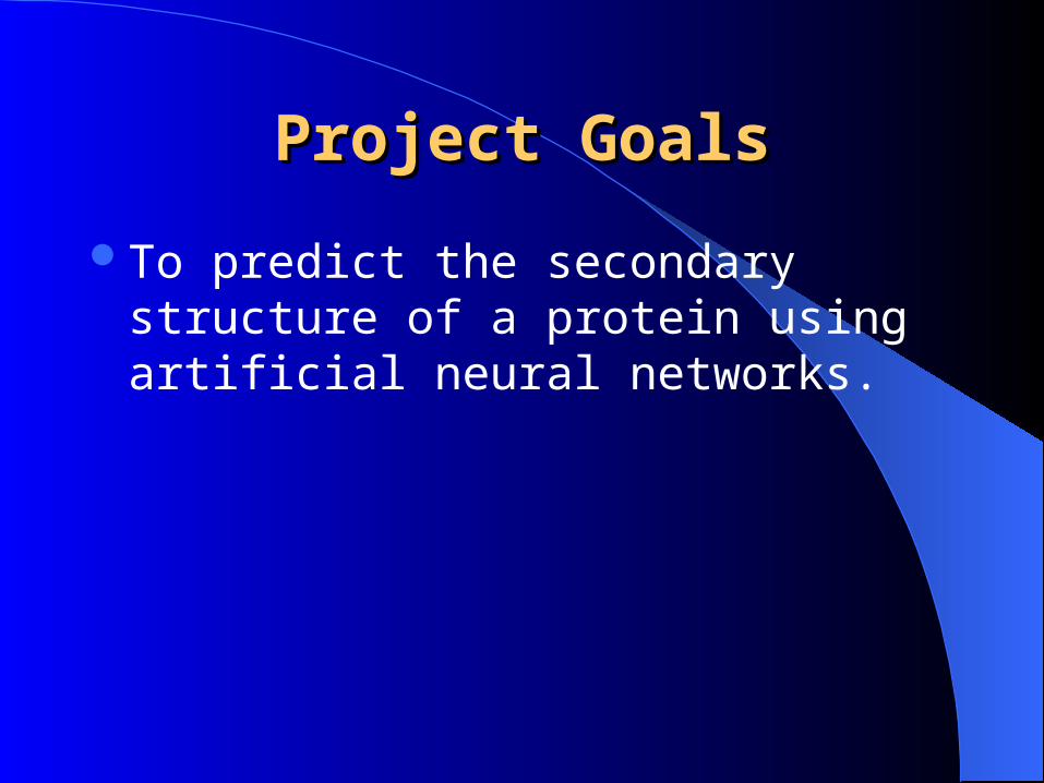
STRUCTURESSTRUCTURES

Primary structure: linear arrangement of amino acid (a.a) residues that constitute the polypeptide chain.

SECONDARY SECONDARY STRUCTURESTRUCTURE

Localized organization of parts of a polypeptide chain, through hydrogen bonds between different residues.

Without any stabilizing interactions , a polypeptide assumes random coil structure.

When stabilizing hydrogen bond forms, the polypeptide backbone folds periodically in to one of two geometric arrangements viz.

ALPHA HELIX BETA SHEET U-TURNS

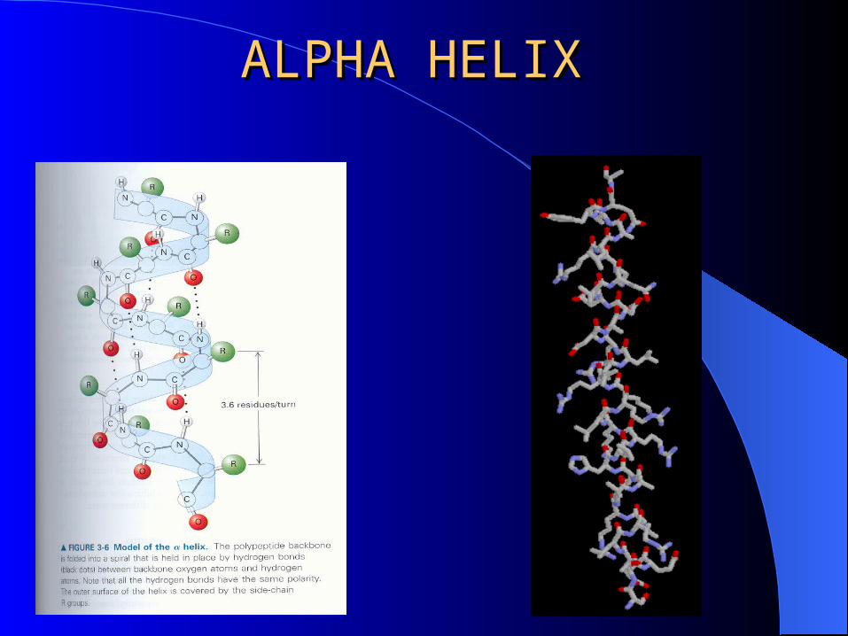
ALPHA HELIXALPHA HELIX A polypeptide back bone is folded in to spiral that is held in place

by hydrogen bonds between backbone oxygen atoms and hydrogen atoms.

The carbonyl oxygen of each peptide bond is hydrogen bonded to the amide hydrogen of the a.a 4 residues toward the C-terminus

Each alpha helix has 3.6 a.a per turn

From the backbone side chains point outward

Hydrophobic/hydrophilic quality of the helix is determined entirely by side chains, because polar groups of the peptide backbone are already involved H-bonding in the helix and thus are unable to affect its hydrophobic/hydrophilic.

ALPHA HELIXALPHA HELIX

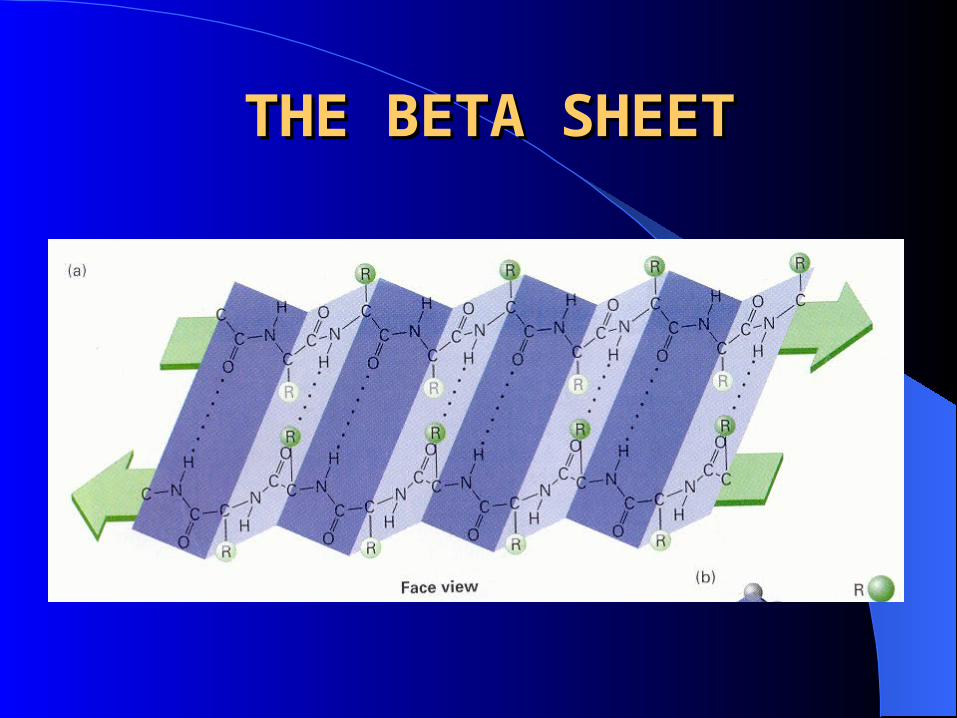
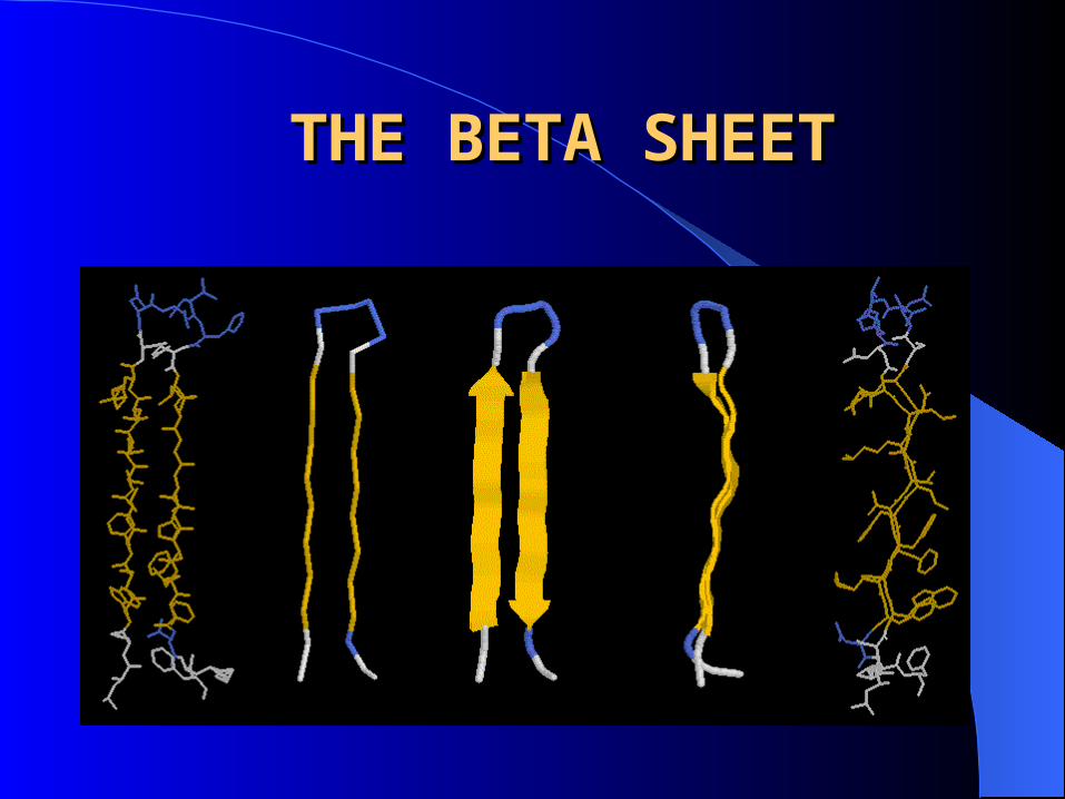
THE BETA SHEETTHE BETA SHEET

Consists of laterally packed beta strands

Each beta strand is a short (5-8 residues), nearly fully extended polypeptide chain

Hydrogen bonding between backbone atoms in a adjacent beta strands, within either the same or different polypeptide chains forms a beta sheet.

Orientation can be either parallel or anti-parallel. In both arrangements side chains project from both faces of the sheet.

THE BETA SHEETTHE BETA SHEET

THE BETA SHEETTHE BETA SHEET

TURNSTURNS

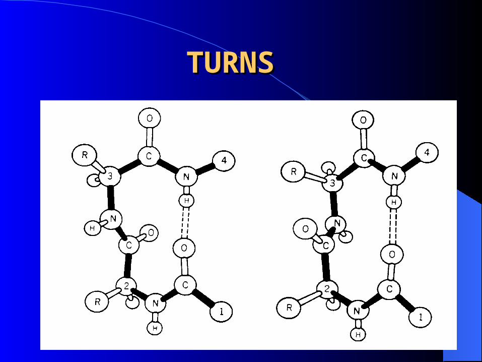
Composed of 3-4 residues , are compact, U-shaped secondary structures stabilized by H-bonds between their end residues.

Located on the surface of the protein, forming a sharp bend that redirects the polypeptide backbone back toward the interior.

Glycine and proline are commonly present. Without these turns , a protein would be large,

extended and loosely packed.

TURNSTURNS

MOTIFS: regular combinations of secondary structure.

– Coiled coil motif

– Helix-loop-helix(Ca+)

– Zinc finger motif.

MOTIFSMOTIFS

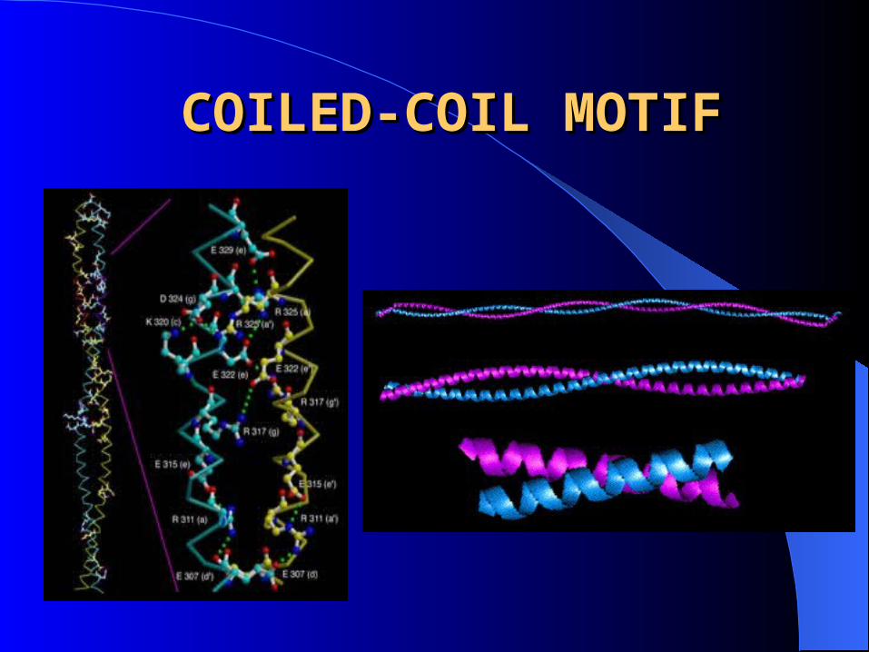
COILED-COIL MOTIFCOILED-COIL MOTIF

                  

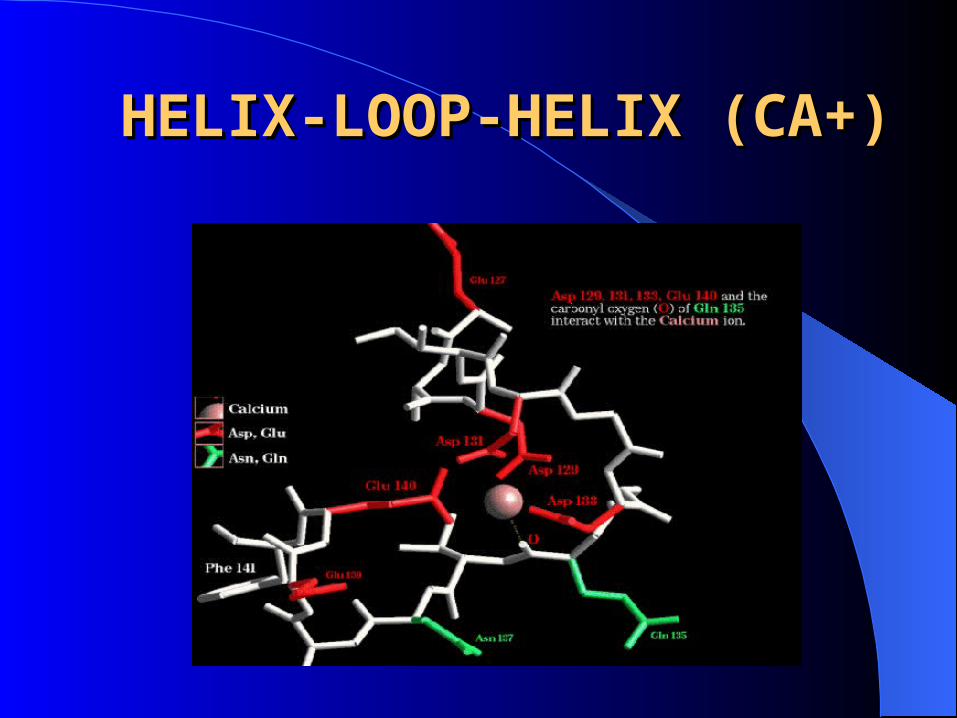
HELIX-LOOP-HELIX (CA+)HELIX-LOOP-HELIX (CA+)

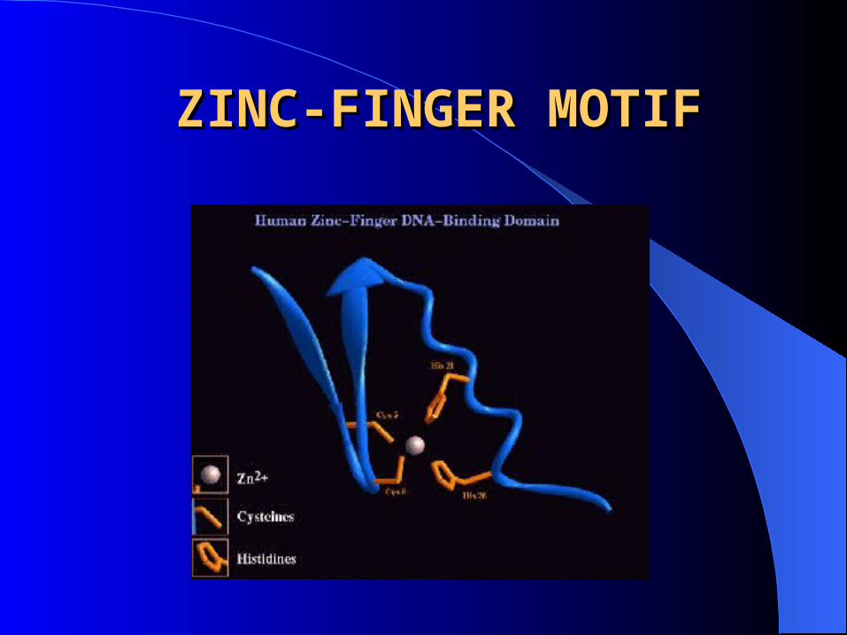
ZINC-FINGER MOTIFZINC-FINGER MOTIF

FUTURE FUTURE Protein structure identification is key to understanding

biological function and its role in health and disease

Characterizing a protein structure helpful in the development of new agents and devices to treat disease

Challenge of unraveling the structure lies in developing methods for accurately and reliably understanding this relationship

Most of the current protein structures have been characterized by NMR and X-Ray diffraction

Revolution in sequencing studies-growing data base-only 3000 known structures

Very few confirmations of protein are possible and structure and sequence are directly related to each other, we can unravel the secondary structure by developing an efficient algorithm, which compares new sequences with the ones available, and use them in health care industry.

ADVANTAGEADVANTAGE

Prediction of secondary structure is an essential intermediate step on the way to predicting the full 3-D structure of a protein

If the secondary structure of a protein is known, it is possible to derive a comparatively small number of possible tertiary structures using knowledge about the ways that secondary structural elements pack

WHY SECONDARY STRUCTURE?WHY SECONDARY STRUCTURE?

Artificial Neural Network Artificial Neural Network (ANN)(ANN)

Peichung Shih

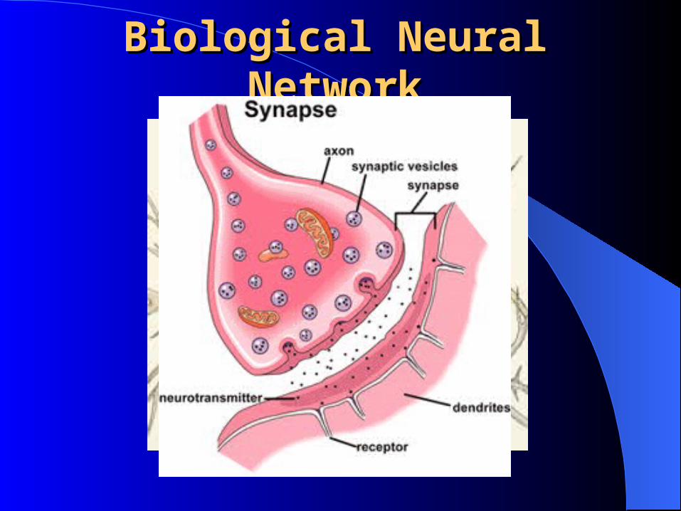
Biological Neural Biological Neural NetworkNetwork

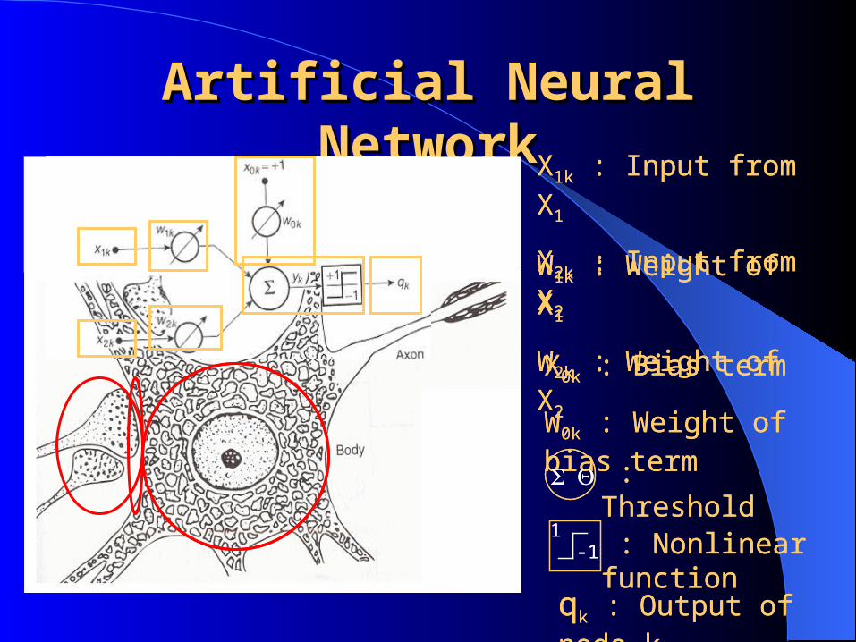
Artificial Neural Artificial Neural NetworkNetwork

: Threshold

X1k : Input from X1

X2k : Input from X2

W1k : Weight of X1

W2k : Weight of X2

X0k : Bias term

W0k : Weight of bias term

-11

: Nonlinear function

qk : Output of node k

X1k : Input from X1

X2k : Input from X2

W1k : Weight of X1

W2k : Weight of X2

X0k : Bias term

W0k : Weight of bias term : Threshold

-1 : Nonlinear function

qk : Output of node k

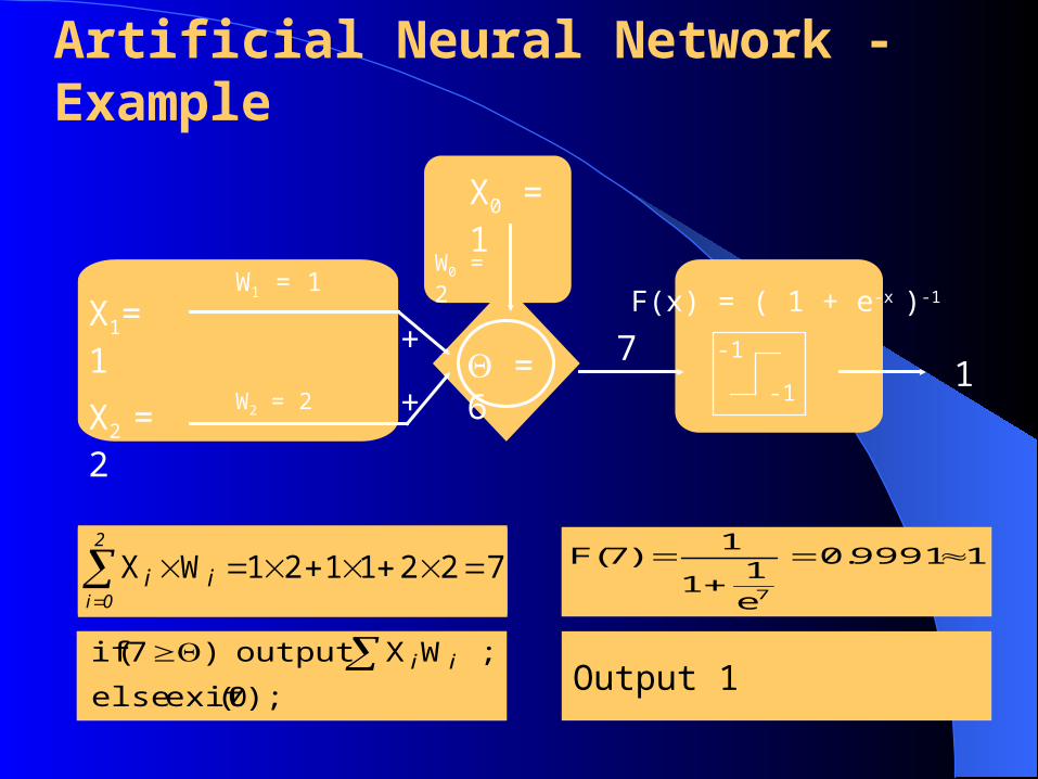
19991.0

e

11

1)7(F

7

);0(exitelse

;WXoutput)7(if ii

7221121WX

2

0iii

Artificial Neural Network - Example

71

7221121WX

2

0iii

);0(exitelse

;WXoutput)7(if ii

W1 = 1X1= 1

W2 = 2X2 = 2

+

+ = 6

X0 = 1

W0 = 2

-1

-1

F(x) = ( 1 + e-x )-1

19991.0

e

11

1)7(F

7

Output 1

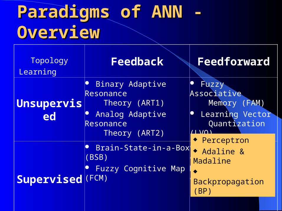
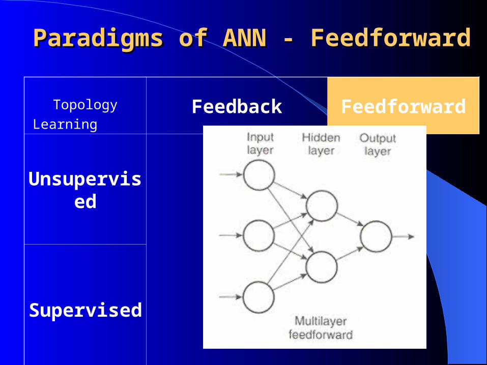
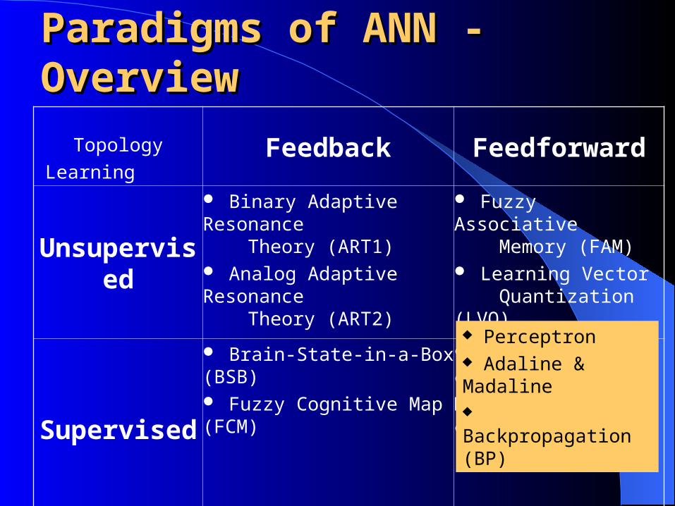
Topology

LearningFeedback Feedforward

Unsupervised

Binary Adaptive Resonance Theory (ART1) Analog Adaptive Resonance Theory (ART2)

Fuzzy Associative Memory (FAM) Learning Vector Quantization (LVQ)

Supervised

Brain-State-in-a-Box (BSB) Fuzzy Cognitive Map (FCM)

Perceptron Adaline & Madaline Backpropagation (BP)

Perceptron Adaline & Madaline Backpropagation (BP)

Paradigms of ANN - Paradigms of ANN - OverviewOverview

Topology

LearningFeedback Feedforward

Unsupervised

Supervised

Paradigms of ANN - Paradigms of ANN - FeedforwardFeedforward

Topology

LearningFeedback Feedforward

Unsupervised

Supervised

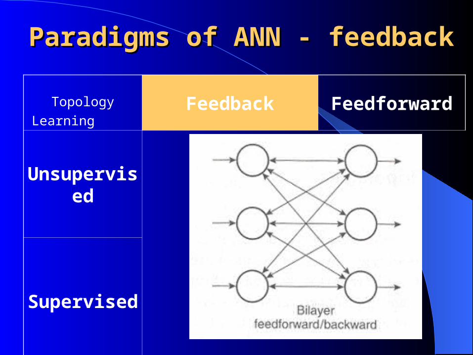
Paradigms of ANN - Paradigms of ANN - feedbackfeedback

Topology

LearningFeedback Feedforward

Unsupervised

Supervised

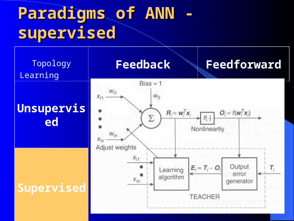
Paradigms of ANN - Paradigms of ANN - supervisedsupervised

Topology

LearningFeedback Feedforward

Unsupervised

Supervised

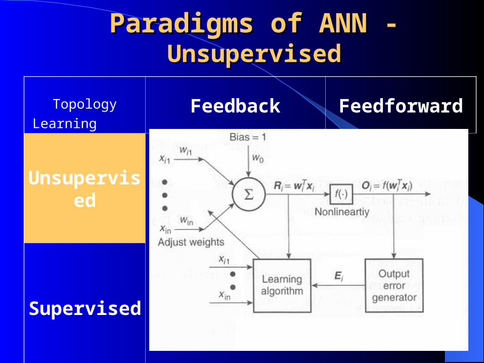
Paradigms of ANN - Paradigms of ANN - UnsupervisedUnsupervised

Topology

LearningFeedback Feedforward

Unsupervised

Binary Adaptive Resonance Theory (ART1) Analog Adaptive Resonance Theory (ART2)

Fuzzy Associative Memory (FAM) Learning Vector Quantization (LVQ)

Supervised

Brain-State-in-a-Box (BSB) Fuzzy Cognitive Map (FCM)

Perceptron Adaline & Madaline Backpropagation (BP)

Perceptron Adaline & Madaline Backpropagation (BP)

Paradigms of ANN - Paradigms of ANN - OverviewOverview

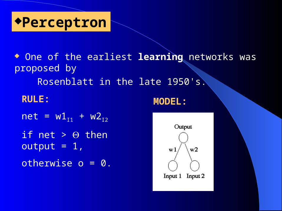
Perceptron One of the earliest learning networks was proposed by Rosenblatt in the late 1950's.

RULE:

net = w1I1 + w2I2

if net > then output = 1,

otherwise o = 0.

MODEL:

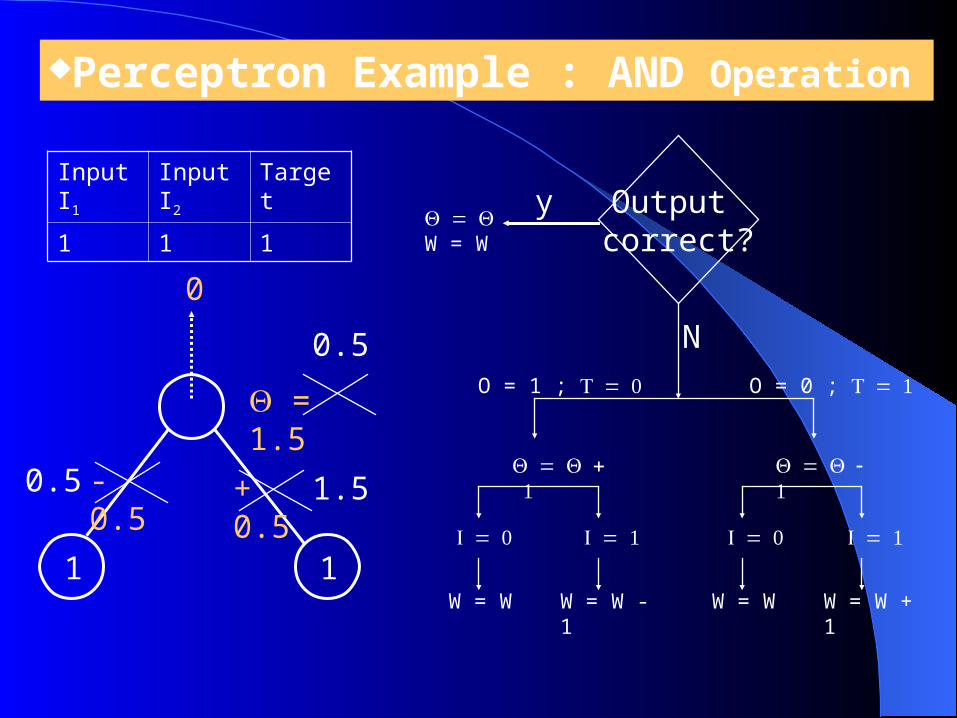
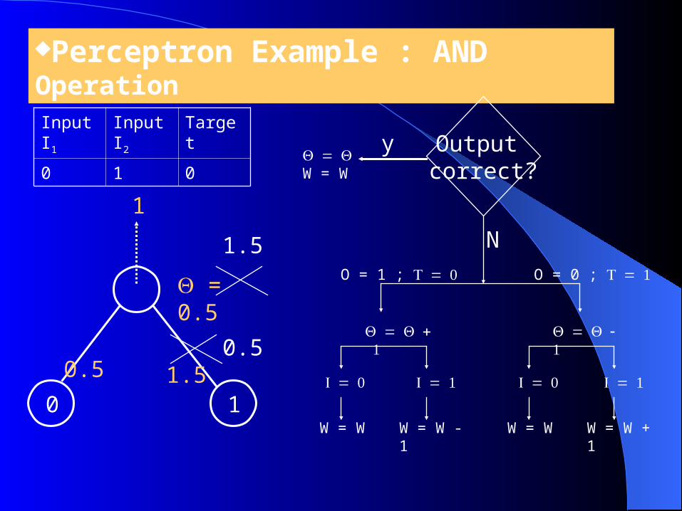
Perceptron Example : AND Operation

Initial Network:

1 1

- 0.5

+ 0.5

= 1.5

W = W + 1

Output correct?

y

NO = 1 ; O = 0 ;

W = W

W = W - 1

W = W

W = W

Perceptron Example : AND Operation

W = W + 1

Output correct?

y

NO = 1 ; O = 0 ;

W = W

W = W - 1

W = W

W = W

= 1.5

1 1

- 0.5

+ 0.5

0

Input I1

Input I2

Target

1 1 1

0.5

0.5 1.5

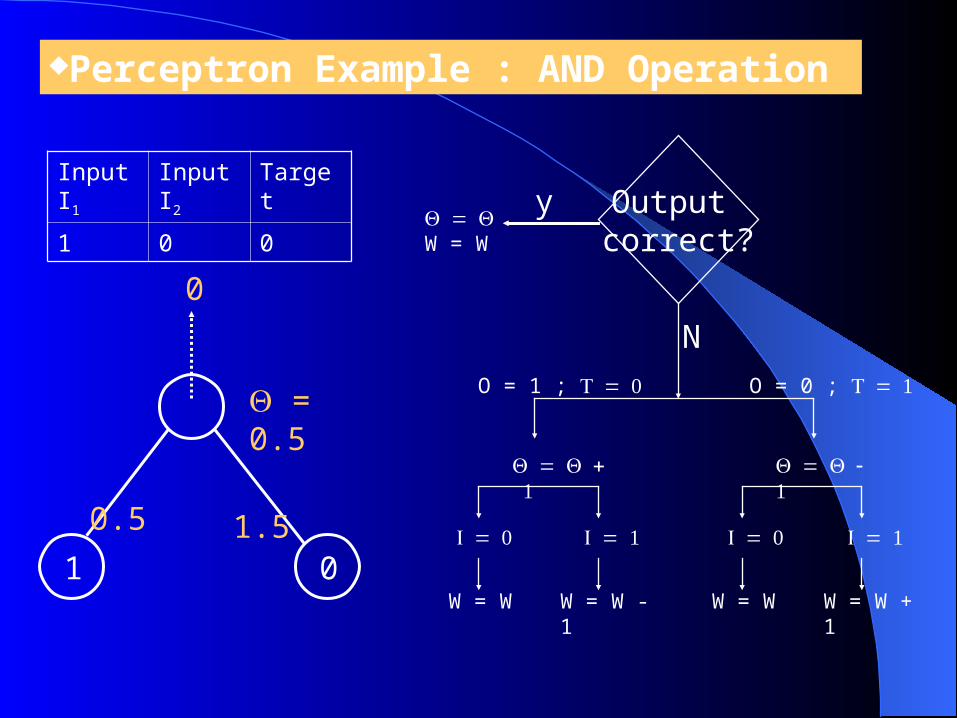
Perceptron Example : AND Operation

W = W + 1

Output correct?

y

NO = 1 ; O = 0 ;

W = W

W = W - 1

W = W

W = W

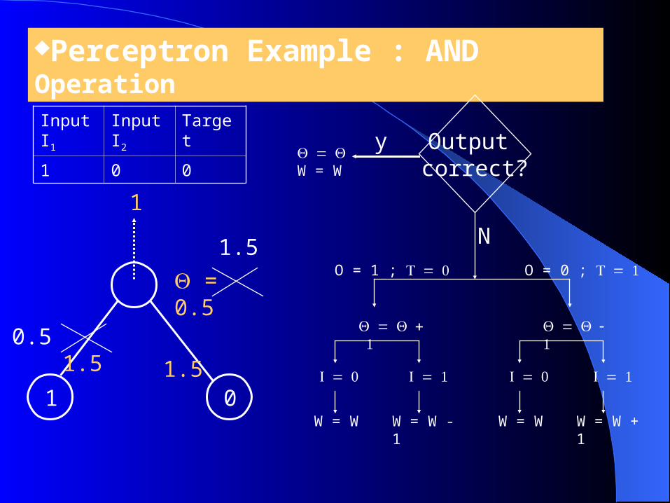
= 0.5

1 0

0.5

1.5

0

Input I1

Input I2

Target

1 0 0

Perceptron Example : AND Operation

W = W + 1

Output correct?

y

NO = 1 ; O = 0 ;

W = W

W = W - 1

W = W

W = W

= 0.5

0 1

0.5

1.5

1

Input I1

Input I2

Target

0 1 0

1.5

0.5

Perceptron Example : AND Operation

W = W + 1

Output correct?

y

NO = 1 ; O = 0 ;

W = W

W = W - 1

W = W

W = W

= 1.5

0 0

0.5

0.5

0

Input I1

Input I2

Target

0 0 0

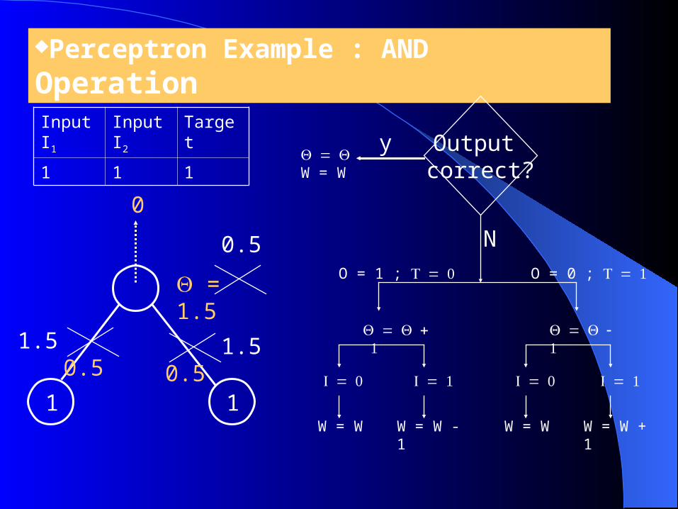
Perceptron Example : AND Operation

W = W + 1

Output correct?

y

NO = 1 ; O = 0 ;

W = W

W = W - 1

W = W

W = W

= 1.5

1 1

0.5

0.5

0

Input I1

Input I2

Target

1 1 1

0.5

1.5 1.5

Perceptron Example : AND Operation

W = W + 1

Output correct?

y

NO = 1 ; O = 0 ;

W = W

W = W - 1

W = W

W = W

= 0.5

1 0

1.5

1.5

1

Input I1

Input I2

Target

1 0 0

1.5

0.5

Perceptron Example : AND Operation

W = W + 1

Output correct?

y

NO = 1 ; O = 0 ;

W = W

W = W - 1

W = W

W = W

= 1.5

0 1

0.5

1.5

0

Input I1

Input I2

Target

0 1 0

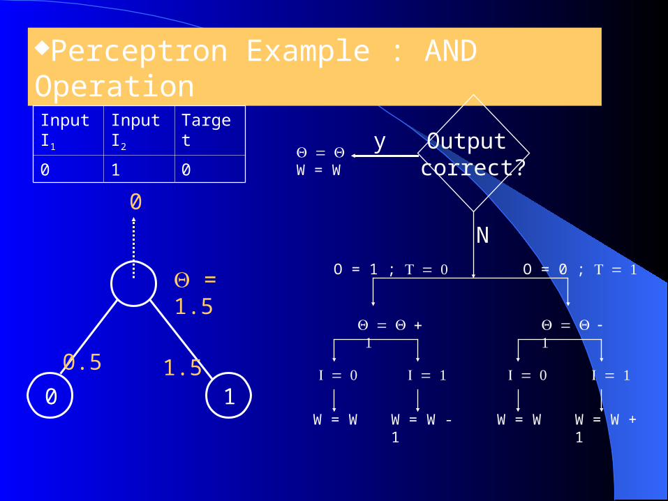
Perceptron Example : AND Operation

W = W + 1

Output correct?

y

NO = 1 ; O = 0 ;

W = W

W = W - 1

W = W

W = W

= 1.5

0 1

0.5

1.5

0

Input I1

Input I2

Target

0 1 0

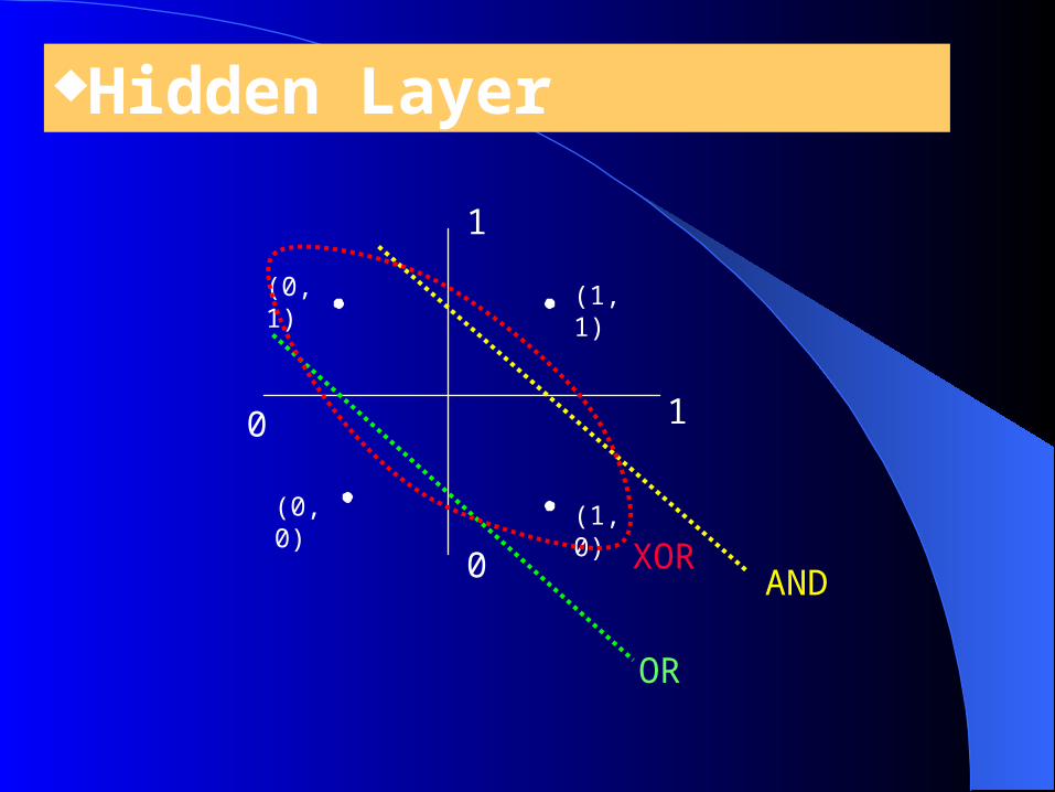
Hidden Layer

10

1

0

(1, 1)

(1, 0)

(0, 1)

(0, 0)

AND

OR

XOR

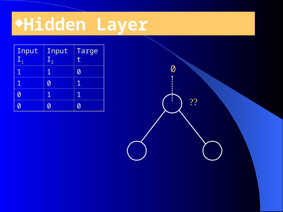
Hidden LayerInput I1

Input I2

Target

1 1 0

1 0 1

0 1 1

0 0 0

0

Hidden LayerInput I1

Input I2

Target

1 1 0

1 0 1

0 1 1

0 0 0

1 1

1 1- 2

1 1 1 1

1 1

1.5

0.5

How Many Hidden How Many Hidden Nodes?Nodes?

We have indicated the number of layers needed. However, no indication is provided as to the optimal number of nodes per layer. There is no formal method to determine this optimal number; typically, one uses trial and error.

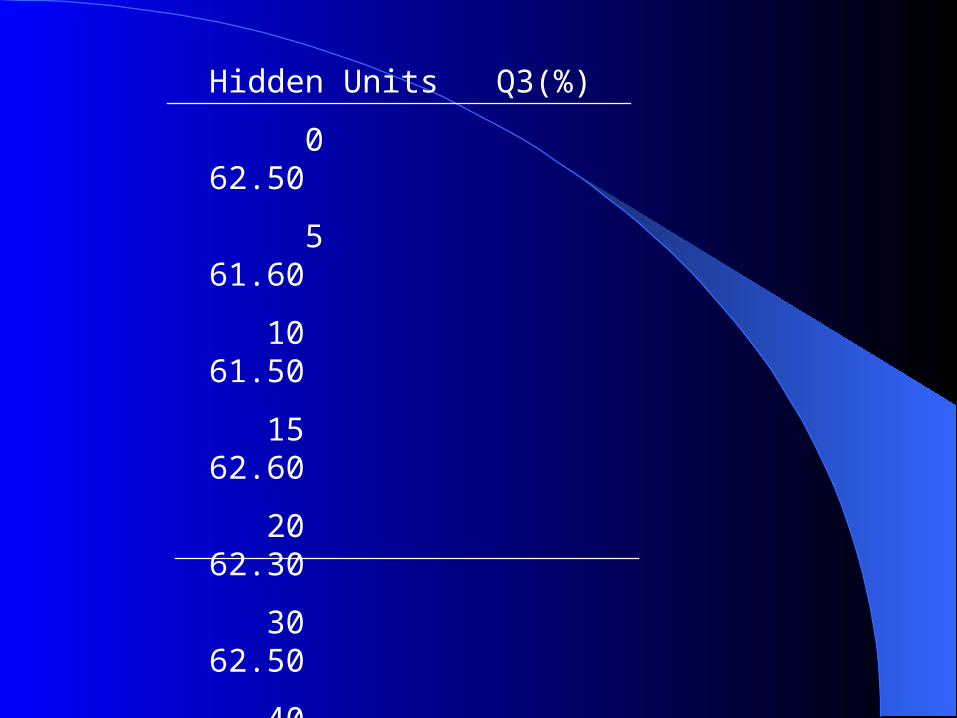
Hidden Units Q3(%)

0 62.50

5 61.60

10 61.50

15 62.60

20 62.30

30 62.50

40 62.70

60 61.40

CHRISSY ORIOL

JNET AND JPRED

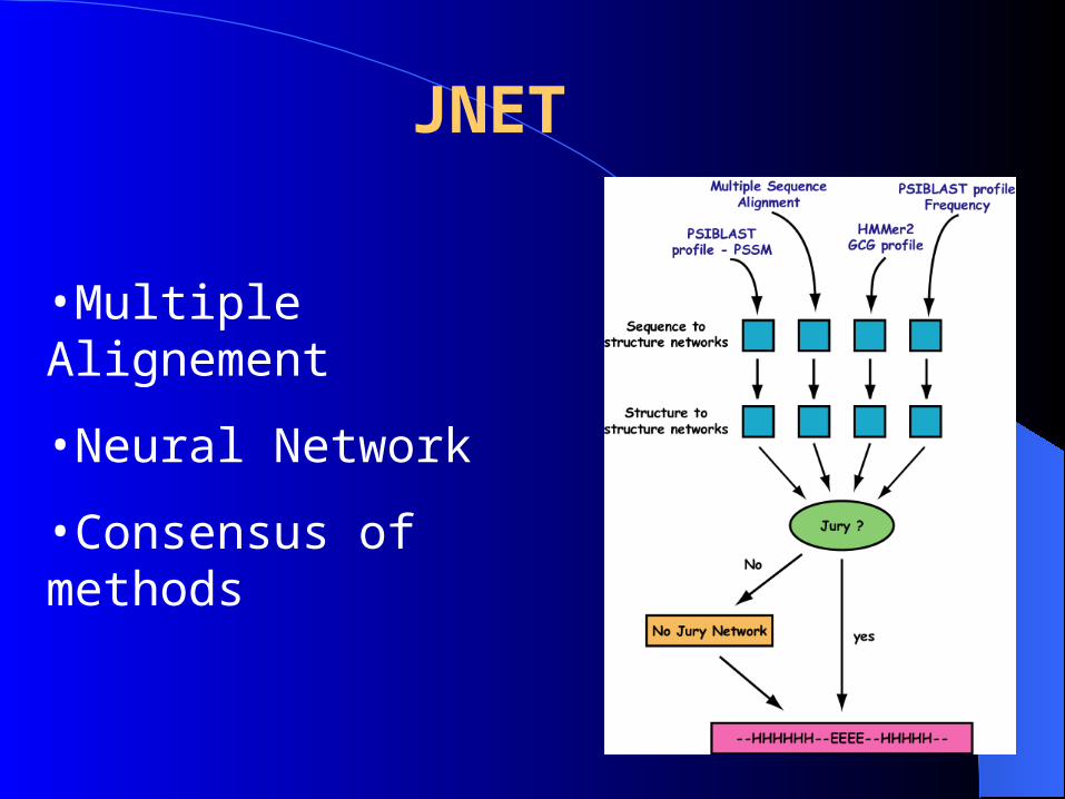
•Multiple Alignement

•Neural Network

•Consensus of methods

JNET

TRAINING AND TESTS

• 480 proteins train (1996 PDB)

• 406 proteins test (2000 PDB)

Blind test

7-fold cross validation test

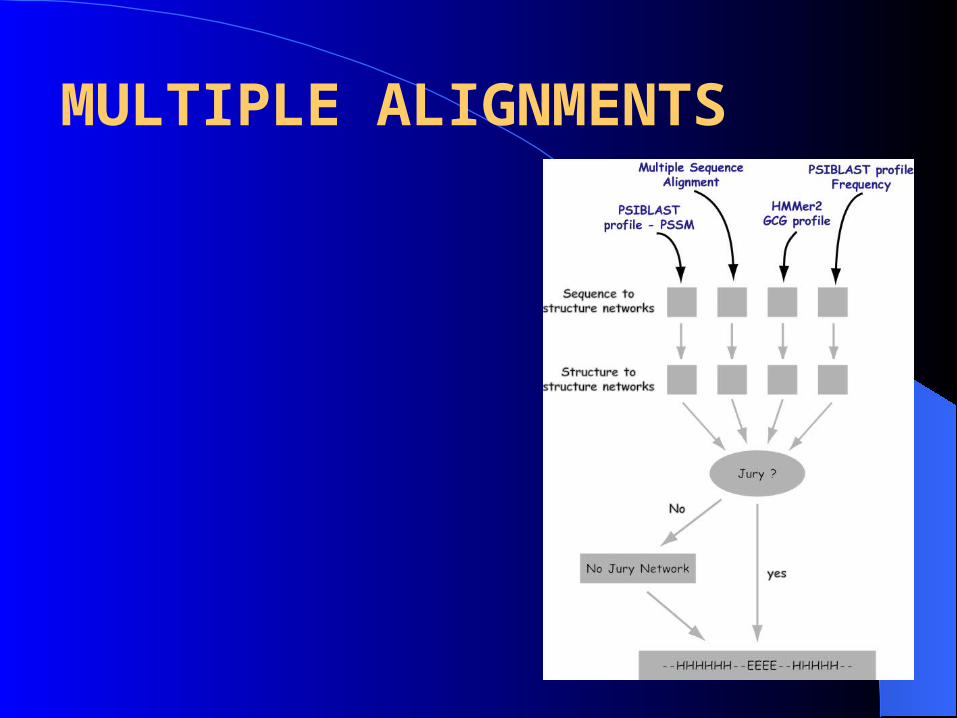
MULTIPLE ALIGNMENTS

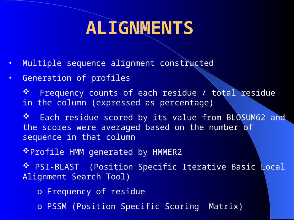
• Multiple sequence alignment constructed

• Generation of profiles

Frequency counts of each residue / total residue in the column (expressed as percentage)

Each residue scored by its value from BLOSUM62 and the scores were averaged based on the number of sequence in that column

Profile HMM generated by HMMER2

PSI-BLAST (Position Specific Iterative Basic Local Alignment Search Tool)

o Frequency of residue

o PSSM (Position Specific Scoring Matrix)

ALIGNMENTS

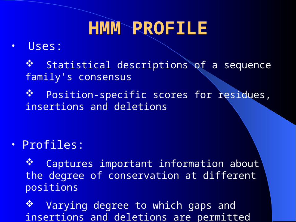
HMM PROFILE• Uses:

Statistical descriptions of a sequence family's consensus

Position-specific scores for residues, insertions and deletions

• Profiles: Captures important information about the degree of conservation at different positions

Varying degree to which gaps and insertions and deletions are permitted

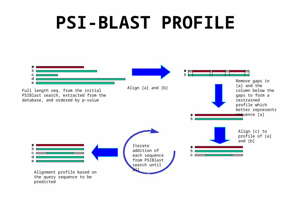
Align [a] and [b]

Remove gaps in [a] and the column below the gaps to form a restrained profile which better represents sequence [a]

Align [c] to profile of [a] and [b]

Iterate addition of each sequence from PSIBlast search until all are aligned

Alignment profile based on the query sequence to be predicted

Full length seq. from the initial PSIBlast search, extracted from the database, and ordered by p-value

PSI-BLAST PROFILE

PSI-BLAST PROFILE

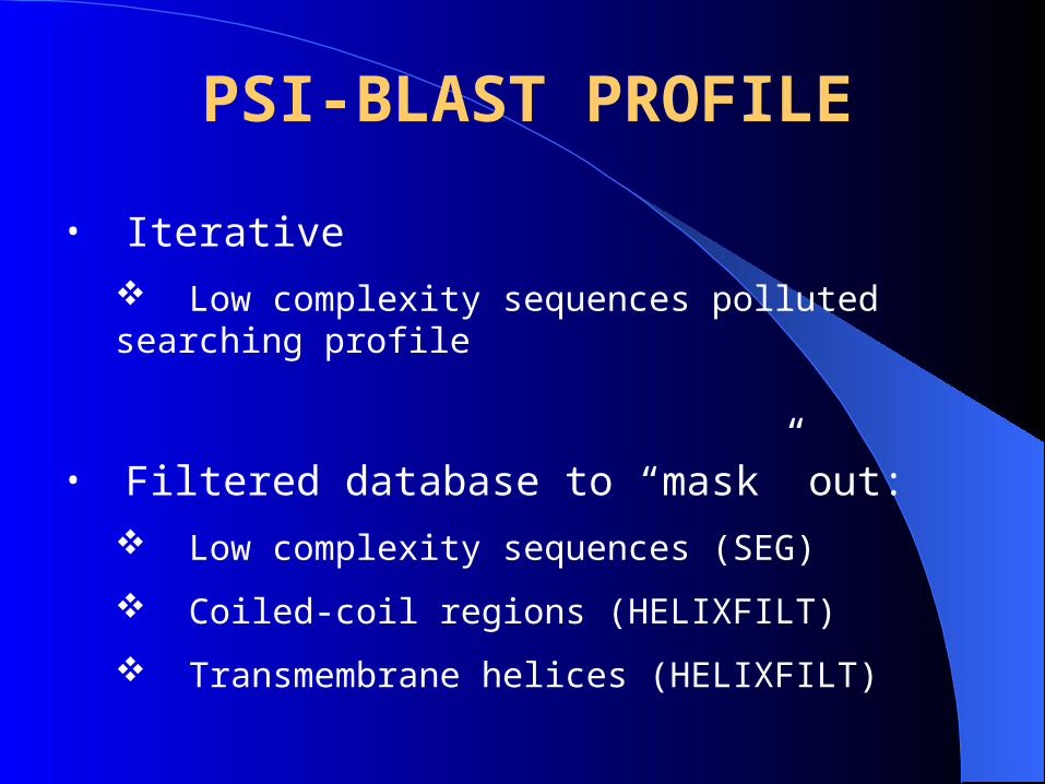
• Iterative Low complexity sequences polluted searching profile

• Filtered database to “mask” out: Low complexity sequences (SEG)

Coiled-coil regions (HELIXFILT)

Transmembrane helices (HELIXFILT)

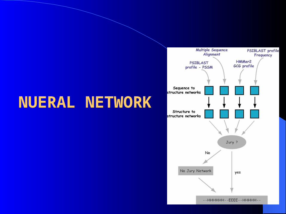
NUERAL NETWORK

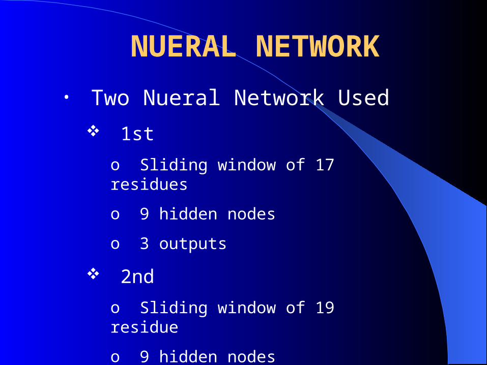
• Two Nueral Network Used 1st

o Sliding window of 17 residues

o 9 hidden nodes

o 3 outputs

2nd

o Sliding window of 19 residue

o 9 hidden nodes

o 3 outputs

NUERAL NETWORK

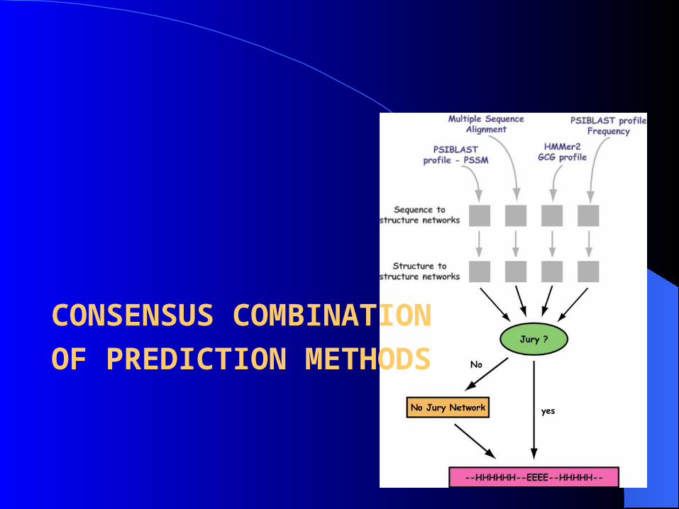
CONSENSUS COMBINATIONOF PREDICTION METHODS

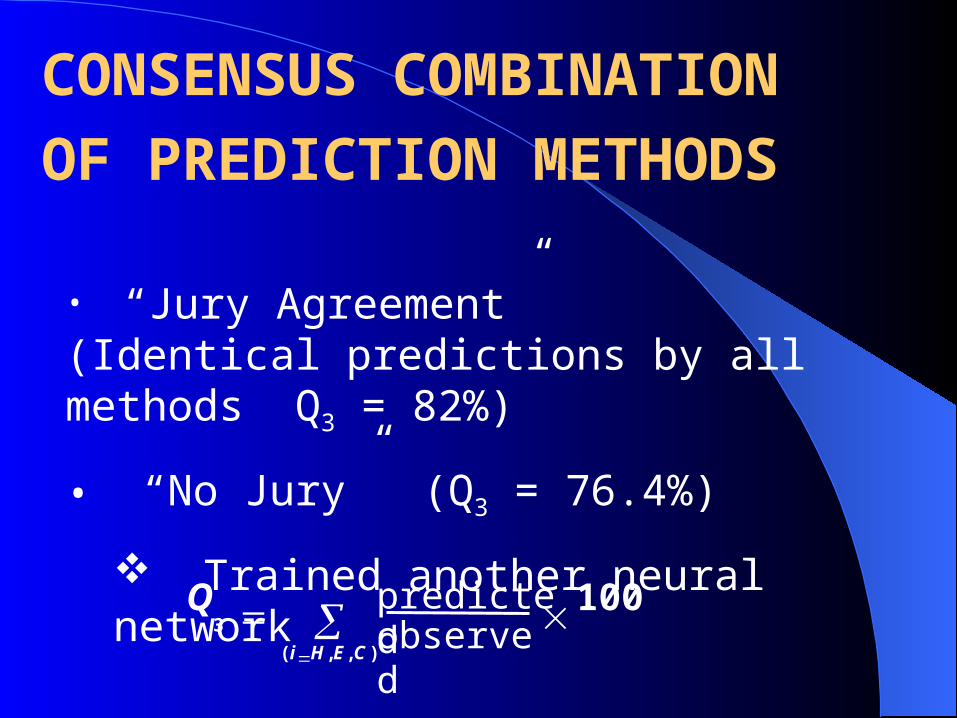
CONSENSUS COMBINATIONOF PREDICTION METHODS

• “Jury Agreement” (Identical predictions by all methods Q3 = 82%)

• “No Jury” (Q3 = 76.4%)

Trained another neural network

Q3

(iH ,E ,C ) 100predicted

observed

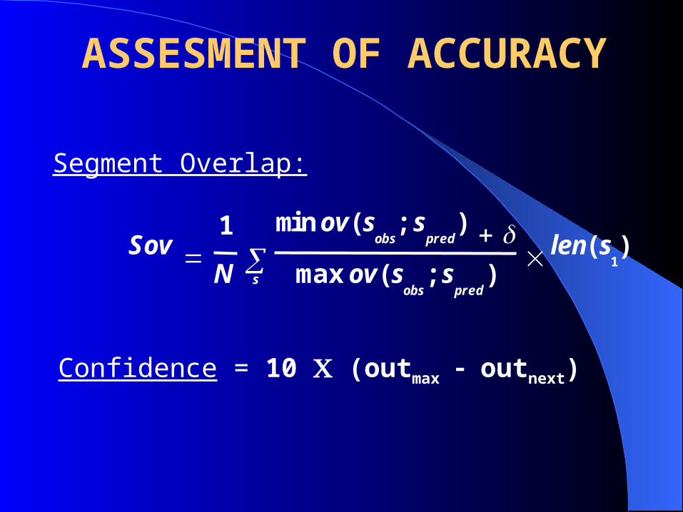
ASSESMENT OF ACCURACY

Confidence = 10 (outmax outnext)

Sov 1

N

minov(sobs

;spred

) maxov(s

obs;s

pred)

len(s1)

s

Segment Overlap:

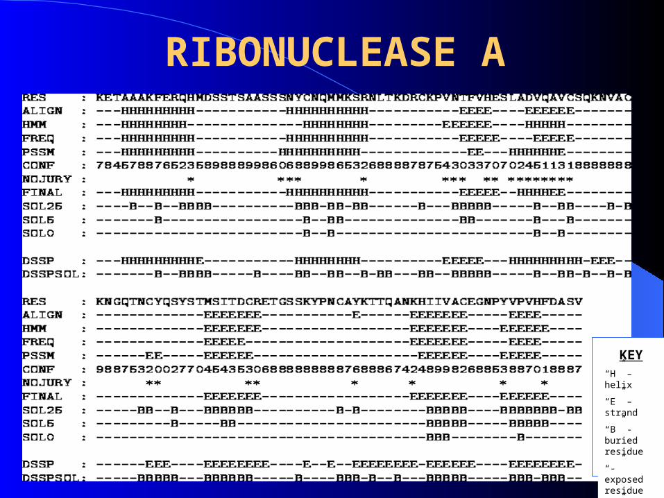
RIBONUCLEASE A

KEY“H” – helix

“E” – strand

“B” - buried residue

“-” exposed residue

“*” – no jury

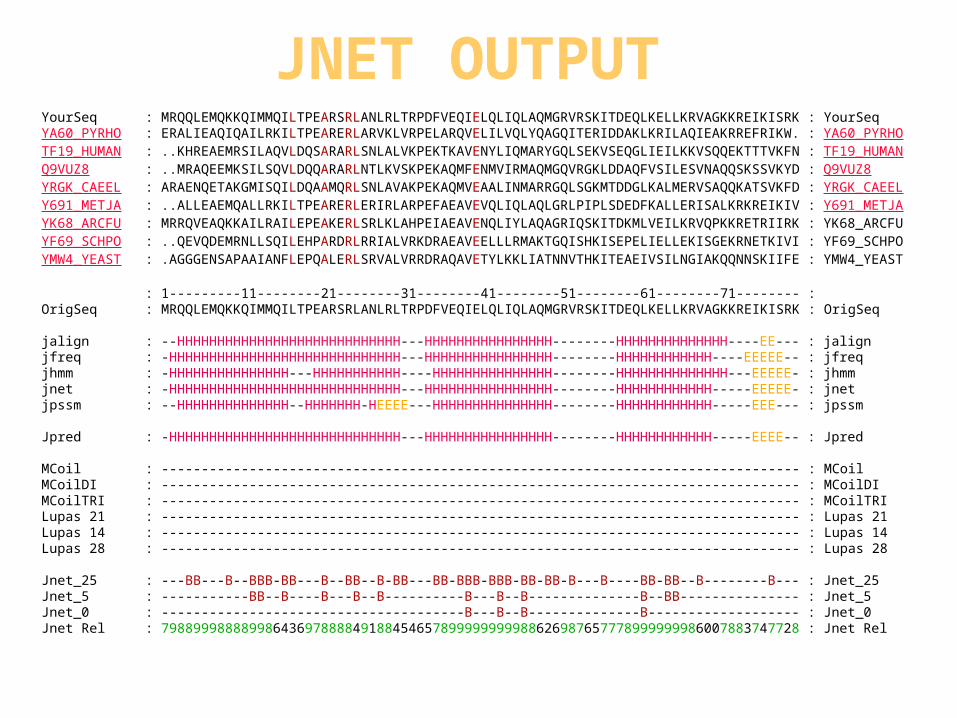
YourSeq : MRQQLEMQKKQIMMQILTPEARSRLANLRLTRPDFVEQIELQLIQLAQMGRVRSKITDEQLKELLKRVAGKKREIKISRK : YourSeq YA60_PYRHO : ERALIEAQIQAILRKILTPEARERLARVKLVRPELARQVELILVQLYQAGQITERIDDAKLKRILAQIEAKRREFRIKW. : YA60_PYRHO TF19_HUMAN : ..KHREAEMRSILAQVLDQSARARLSNLALVKPEKTKAVENYLIQMARYGQLSEKVSEQGLIEILKKVSQQEKTTTVKFN : TF19_HUMAN Q9VUZ8 : ..MRAQEEMKSILSQVLDQQARARLNTLKVSKPEKAQMFENMVIRMAQMGQVRGKLDDAQFVSILESVNAQQSKSSVKYD : Q9VUZ8 YRGK_CAEEL : ARAENQETAKGMISQILDQAAMQRLSNLAVAKPEKAQMVEAALINMARRGQLSGKMTDDGLKALMERVSAQQKATSVKFD : YRGK_CAEEL Y691_METJA : ..ALLEAEMQALLRKILTPEARERLERIRLARPEFAEAVEVQLIQLAQLGRLPIPLSDEDFKALLERISALKRKREIKIV : Y691_METJA YK68_ARCFU : MRRQVEAQKKAILRAILEPEAKERLSRLKLAHPEIAEAVENQLIYLAQAGRIQSKITDKMLVEILKRVQPKKRETRIIRK : YK68_ARCFU YF69_SCHPO : ..QEVQDEMRNLLSQILEHPARDRLRRIALVRKDRAEAVEELLLRMAKTGQISHKISEPELIELLEKISGEKRNETKIVI : YF69_SCHPO YMW4_YEAST : .AGGGENSAPAAIANFLEPQALERLSRVALVRRDRAQAVETYLKKLIATNNVTHKITEAEIVSILNGIAKQQNNSKIIFE : YMW4_YEAST   : 1---------11--------21--------31--------41--------51--------61--------71-------- :OrigSeq : MRQQLEMQKKQIMMQILTPEARSRLANLRLTRPDFVEQIELQLIQLAQMGRVRSKITDEQLKELLKRVAGKKREIKISRK : OrigSeq jalign : --HHHHHHHHHHHHHHHHHHHHHHHHHHHH---HHHHHHHHHHHHHHHH--------HHHHHHHHHHHHHH----EE--- : jalignjfreq : -HHHHHHHHHHHHHHHHHHHHHHHHHHHHH---HHHHHHHHHHHHHHHH--------HHHHHHHHHHHH----EEEEE-- : jfreqjhmm : -HHHHHHHHHHHHHHH---HHHHHHHHHHH----HHHHHHHHHHHHHHH--------HHHHHHHHHHHHHH---EEEEE- : jhmmjnet : -HHHHHHHHHHHHHHHHHHHHHHHHHHHHH---HHHHHHHHHHHHHHHH--------HHHHHHHHHHHH-----EEEEE- : jnetjpssm : --HHHHHHHHHHHHHH--HHHHHHH-HEEEE---HHHHHHHHHHHHHHH--------HHHHHHHHHHHH-----EEE--- : jpssm Jpred : -HHHHHHHHHHHHHHHHHHHHHHHHHHHHH---HHHHHHHHHHHHHHHH--------HHHHHHHHHHHH-----EEEE-- : Jpred MCoil : -------------------------------------------------------------------------------- : MCoilMCoilDI : -------------------------------------------------------------------------------- : MCoilDIMCoilTRI : -------------------------------------------------------------------------------- : MCoilTRILupas 21 : -------------------------------------------------------------------------------- : Lupas 21Lupas 14 : -------------------------------------------------------------------------------- : Lupas 14Lupas 28 : -------------------------------------------------------------------------------- : Lupas 28 Jnet_25 : ---BB---B--BBB-BB---B--BB--B-BB---BB-BBB-BBB-BB-BB-B---B----BB-BB--B--------B--- : Jnet_25Jnet_5 : -----------BB--B----B---B--B----------B---B--B--------------B--BB--------------- : Jnet_5Jnet_0 : --------------------------------------B---B--B--------------B------------------- : Jnet_0Jnet Rel : 79889998888998643697888849188454657899999999988626987657778999999986007883747728 : Jnet Rel

JNET OUTPUT

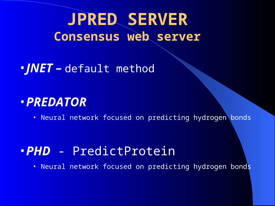
JPRED SERVERConsensus web server

•JNET – default method

•PREDATOR • Neural network focused on predicting hydrogen bonds

•PHD - PredictProtein • Neural network focused on predicting hydrogen bonds

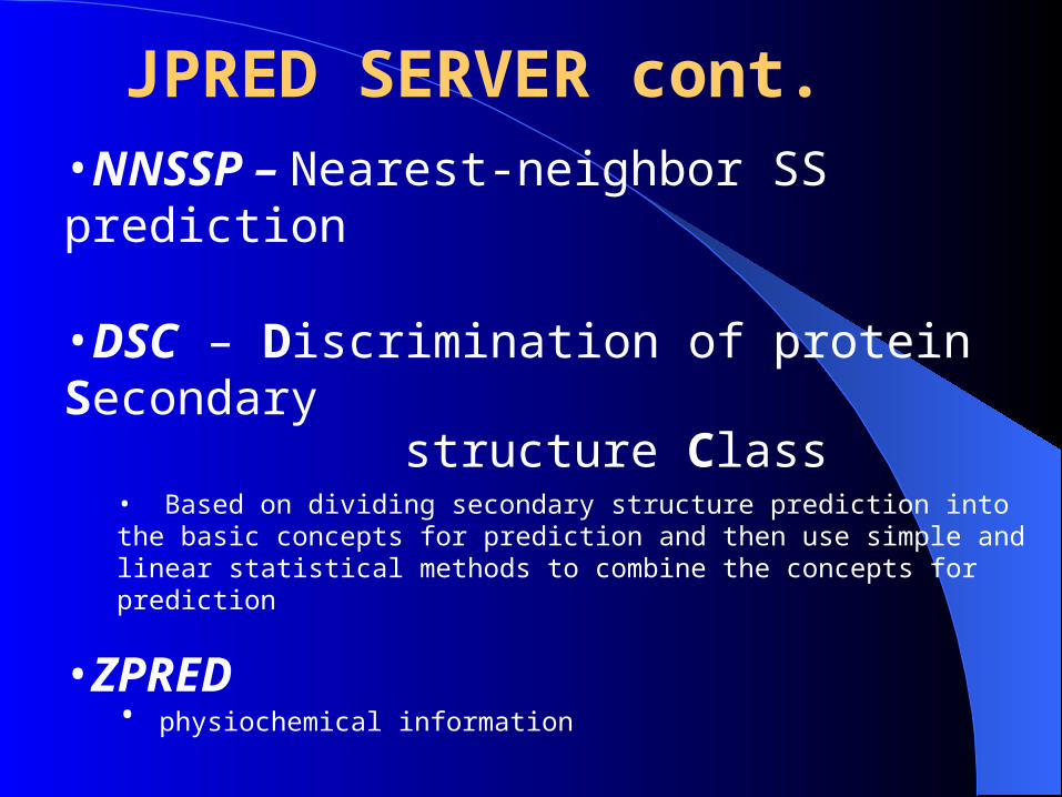
•NNSSP – Nearest-neighbor SS prediction

•DSC – Discrimination of protein Secondary structure Class

• Based on dividing secondary structure prediction into the basic concepts for prediction and then use simple and linear statistical methods to combine the concepts for prediction

•ZPRED• physiochemical information

•MULPRED •Single sequence method combination

JPRED SERVER cont.

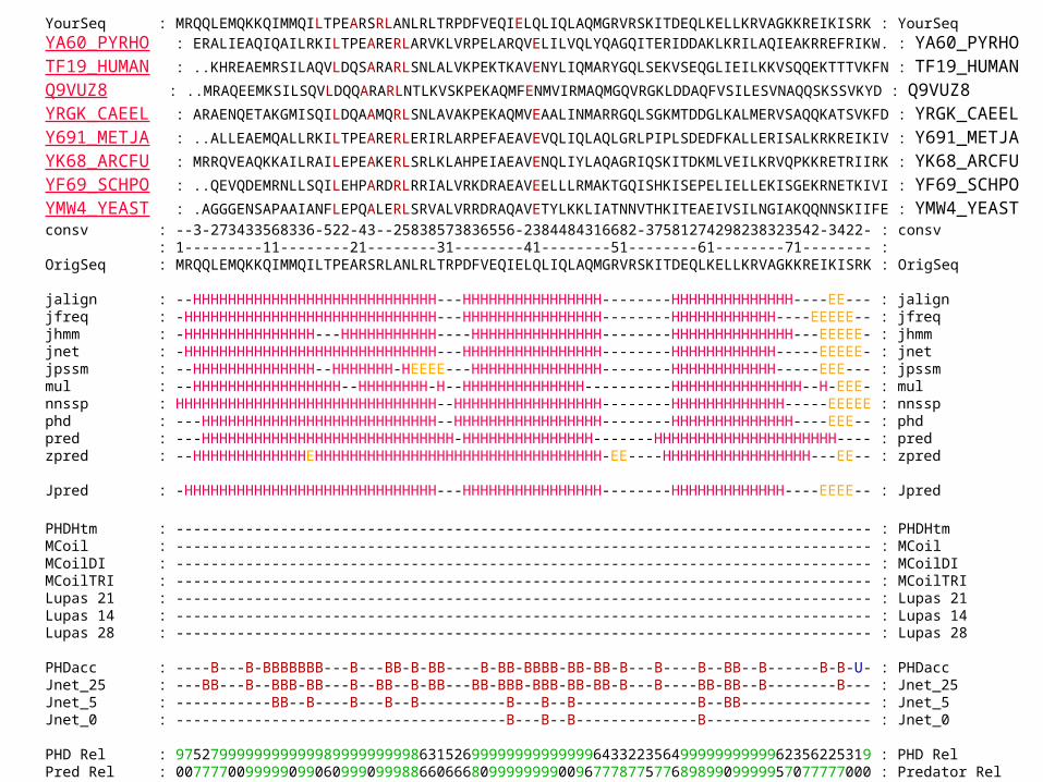
YourSeq : MRQQLEMQKKQIMMQILTPEARSRLANLRLTRPDFVEQIELQLIQLAQMGRVRSKITDEQLKELLKRVAGKKREIKISRK : YourSeq YA60_PYRHO : ERALIEAQIQAILRKILTPEARERLARVKLVRPELARQVELILVQLYQAGQITERIDDAKLKRILAQIEAKRREFRIKW. : YA60_PYRHO TF19_HUMAN : ..KHREAEMRSILAQVLDQSARARLSNLALVKPEKTKAVENYLIQMARYGQLSEKVSEQGLIEILKKVSQQEKTTTVKFN : TF19_HUMAN Q9VUZ8 : ..MRAQEEMKSILSQVLDQQARARLNTLKVSKPEKAQMFENMVIRMAQMGQVRGKLDDAQFVSILESVNAQQSKSSVKYD : Q9VUZ8 YRGK_CAEEL : ARAENQETAKGMISQILDQAAMQRLSNLAVAKPEKAQMVEAALINMARRGQLSGKMTDDGLKALMERVSAQQKATSVKFD : YRGK_CAEEL Y691_METJA : ..ALLEAEMQALLRKILTPEARERLERIRLARPEFAEAVEVQLIQLAQLGRLPIPLSDEDFKALLERISALKRKREIKIV : Y691_METJA YK68_ARCFU : MRRQVEAQKKAILRAILEPEAKERLSRLKLAHPEIAEAVENQLIYLAQAGRIQSKITDKMLVEILKRVQPKKRETRIIRK : YK68_ARCFU YF69_SCHPO : ..QEVQDEMRNLLSQILEHPARDRLRRIALVRKDRAEAVEELLLRMAKTGQISHKISEPELIELLEKISGEKRNETKIVI : YF69_SCHPO YMW4_YEAST : .AGGGENSAPAAIANFLEPQALERLSRVALVRRDRAQAVETYLKKLIATNNVTHKITEAEIVSILNGIAKQQNNSKIIFE : YMW4_YEAST consv : --3-273433568336-522-43--25838573836556-2384484316682-37581274298238323542-3422- : consv : 1---------11--------21--------31--------41--------51--------61--------71-------- :OrigSeq : MRQQLEMQKKQIMMQILTPEARSRLANLRLTRPDFVEQIELQLIQLAQMGRVRSKITDEQLKELLKRVAGKKREIKISRK : OrigSeq jalign : --HHHHHHHHHHHHHHHHHHHHHHHHHHHH---HHHHHHHHHHHHHHHH--------HHHHHHHHHHHHHH----EE--- : jalignjfreq : -HHHHHHHHHHHHHHHHHHHHHHHHHHHHH---HHHHHHHHHHHHHHHH--------HHHHHHHHHHHH----EEEEE-- : jfreqjhmm : -HHHHHHHHHHHHHHH---HHHHHHHHHHH----HHHHHHHHHHHHHHH--------HHHHHHHHHHHHHH---EEEEE- : jhmmjnet : -HHHHHHHHHHHHHHHHHHHHHHHHHHHHH---HHHHHHHHHHHHHHHH--------HHHHHHHHHHHH-----EEEEE- : jnetjpssm : --HHHHHHHHHHHHHH--HHHHHHH-HEEEE---HHHHHHHHHHHHHHH--------HHHHHHHHHHHH-----EEE--- : jpssmmul : --HHHHHHHHHHHHHHHHH--HHHHHHHH-H--HHHHHHHHHHHHHH----------HHHHHHHHHHHHHHH--H-EEE- : mulnnssp : HHHHHHHHHHHHHHHHHHHHHHHHHHHHHH--HHHHHHHHHHHHHHHHH--------HHHHHHHHHHHHH-----EEEEE : nnsspphd : ---HHHHHHHHHHHHHHHHHHHHHHHHHHH--HHHHHHHHHHHHHHHHH--------HHHHHHHHHHHHHH----EEE-- : phdpred : ---HHHHHHHHHHHHHHHHHHHHHHHHHHHHH-HHHHHHHHHHHHHHH-------HHHHHHHHHHHHHHHHHHHHH---- : predzpred : --HHHHHHHHHHHHHEHHHHHHHHHHHHHHHHHHHHHHHHHHHHHHHHH-EE----HHHHHHHHHHHHHHHHH---EE-- : zpred Jpred : -HHHHHHHHHHHHHHHHHHHHHHHHHHHHH---HHHHHHHHHHHHHHHH--------HHHHHHHHHHHHH----EEEE-- : Jpred

PHDHtm : -------------------------------------------------------------------------------- : PHDHtmMCoil : -------------------------------------------------------------------------------- : MCoilMCoilDI : -------------------------------------------------------------------------------- : MCoilDIMCoilTRI : -------------------------------------------------------------------------------- : MCoilTRILupas 21 : -------------------------------------------------------------------------------- : Lupas 21Lupas 14 : -------------------------------------------------------------------------------- : Lupas 14Lupas 28 : -------------------------------------------------------------------------------- : Lupas 28 PHDacc : ----B---B-BBBBBBB---B---BB-B-BB----B-BB-BBBB-BB-BB-B---B----B--BB--B------B-B-U- : PHDaccJnet_25 : ---BB---B--BBB-BB---B--BB--B-BB---BB-BBB-BBB-BB-BB-B---B----BB-BB--B--------B--- : Jnet_25Jnet_5 : -----------BB--B----B---B--B----------B---B--B--------------B--BB--------------- : Jnet_5Jnet_0 : --------------------------------------B---B--B--------------B------------------- : Jnet_0 PHD Rel : 97527999999999999899999999986315269999999999999964332235649999999999962356225319 : PHD RelPred Rel : 00777700999990990609990999886606668099999999009677787757768989909999957077777000 : Predator RelJnet Rel : 79889998888998643697888849188454657899999999988626987657778999999986007883747728 : Jnet Rel

Accuracy EvaluationAccuracy Evaluation

By Liang-Yu Shih

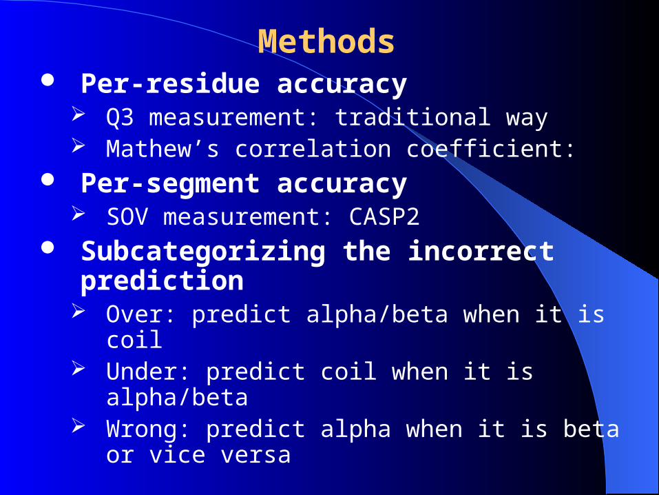
Per-residue accuracy Q3 measurement: traditional way Mathew’s correlation coefficient:

Per-segment accuracy SOV measurement: CASP2

Subcategorizing the incorrect prediction

Over: predict alpha/beta when it is coil Under: predict coil when it is alpha/beta Wrong: predict alpha when it is beta or

vice versa

Methods

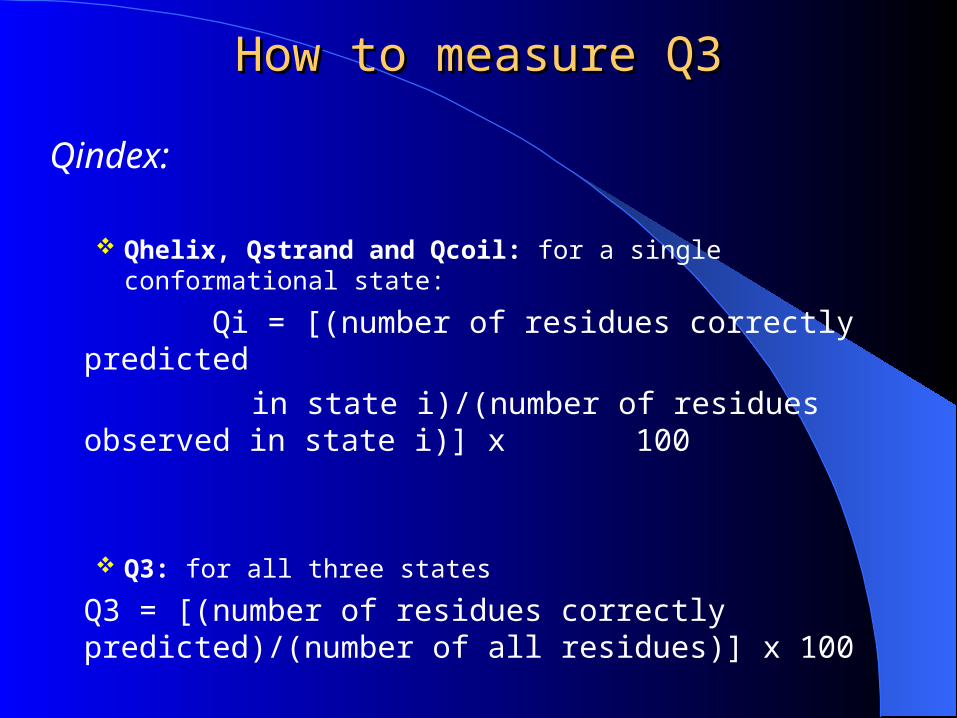
How to measure Q3How to measure Q3

Qindex:

Qhelix, Qstrand and Qcoil: for a single conformational state:

Qi = [(number of residues correctly predicted in state i)/(number of residues observed in

state i)] x 100

Q3: for all three states

Q3 = [(number of residues correctly predicted)/(number of all residues)] x 100

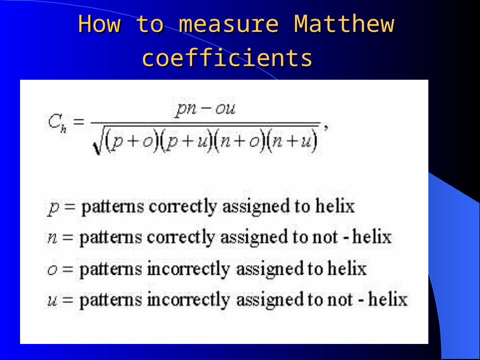
How to measure How to measure MatthewMatthew

coefficientscoefficients

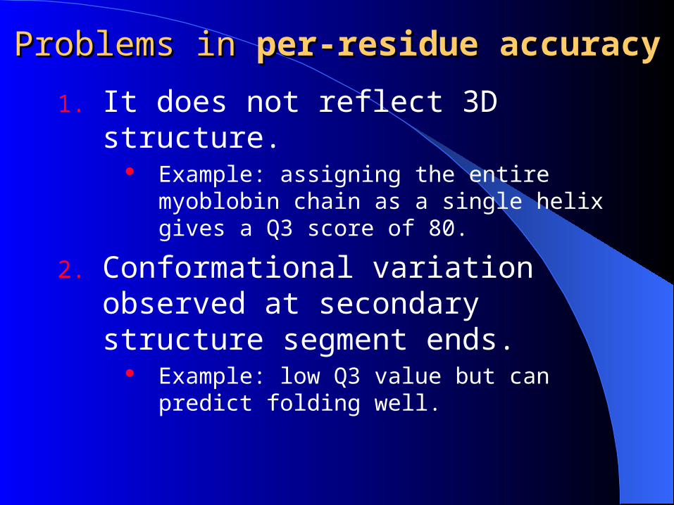
Problems in Problems in per-residue accuracyper-residue accuracy

1. It does not reflect 3D structure. Example: assigning the entire

myoblobin chain as a single helix gives a Q3 score of 80.

2. Conformational variation observed at secondary structure segment ends.

Example: low Q3 value but can predict folding well.

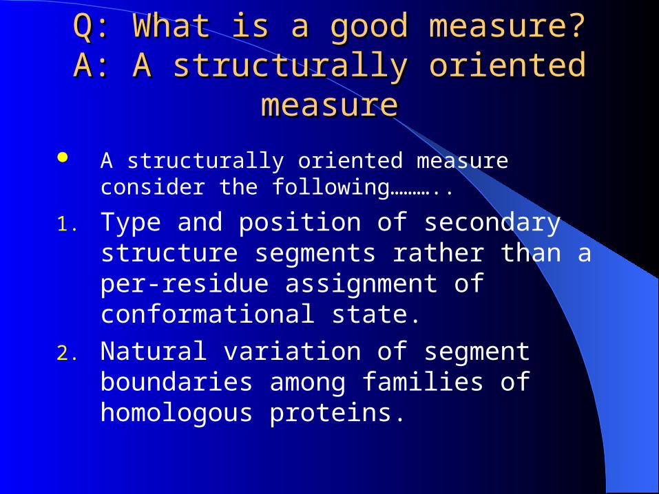
Q: What is a good measure?Q: What is a good measure?A: A structurally oriented A: A structurally oriented

measuremeasure A structurally oriented measure consider the

following………..

1. Type and position of secondary structure segments rather than a per-residue assignment of conformational state.

2. Natural variation of segment boundaries among families of homologous proteins.

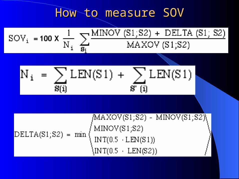
How to measure SOVHow to measure SOV

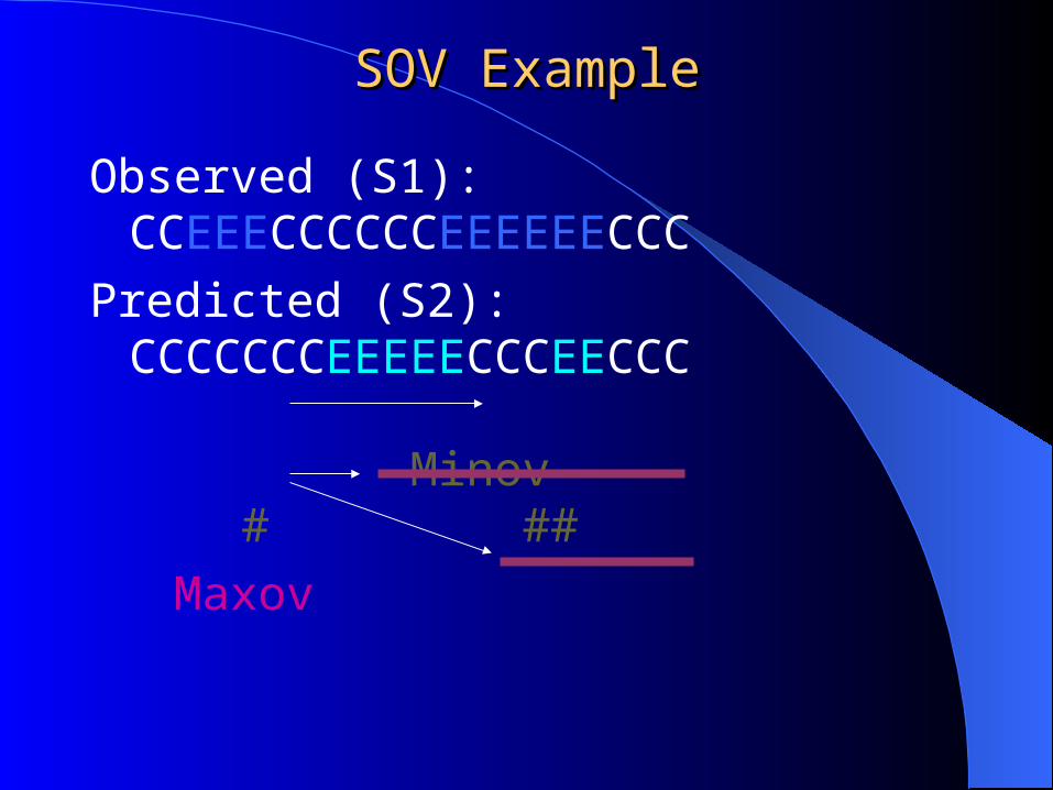
SOV ExampleSOV Example

Observed (S1): CCEEECCCCCCEEEEEECCC

Predicted (S2): CCCCCCCEEEEECCCEECCC Minov # ##

Maxov

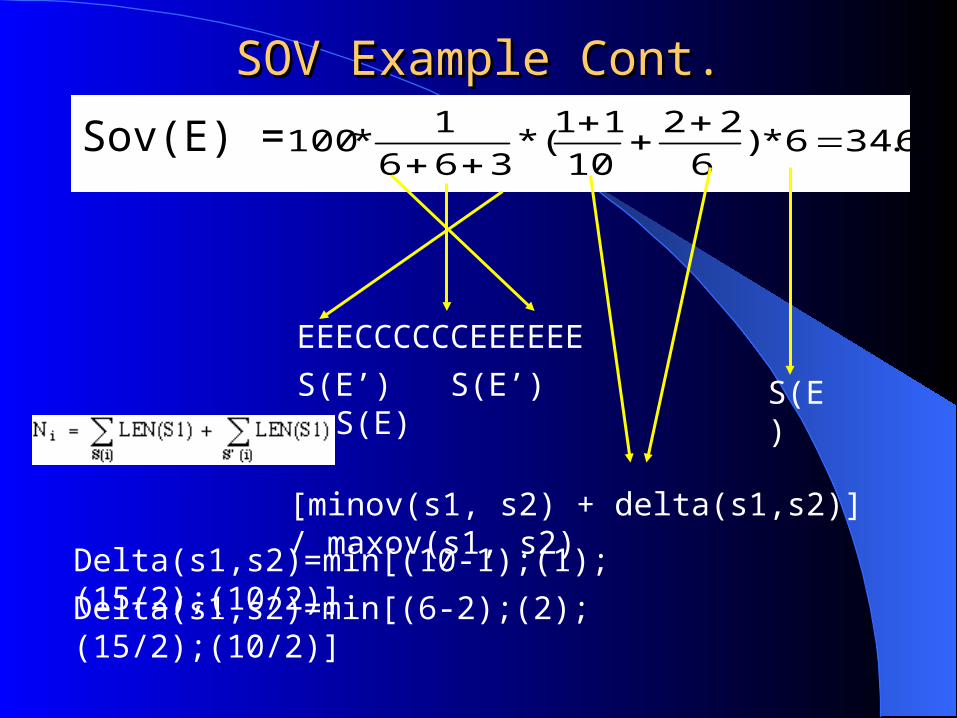
SOV Example Cont.SOV Example Cont.

Sov(E) = 6.346*)6

22

10

11(*

366

1*100

EEECCCCCCEEEEEE

[minov(s1, s2) + delta(s1,s2)] / maxov(s1, s2)

S(E’) S(E’) S(E) S(E)

Delta(s1,s2)=min[(10-1);(1);(15/2);(10/2)]

Delta(s1,s2)=min[(6-2);(2);(15/2);(10/2)]

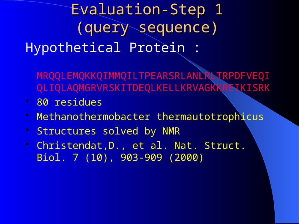
Evaluation-Step 1Evaluation-Step 1(query sequence)(query sequence)

Hypothetical Protein :

MRQQLEMQKKQIMMQILTPEARSRLANLRLTRPDFVEQIQLIQLAQMGRVRSKITDEQLKELLKRVAGKKREIKISRK

80 residues Methanothermobacter thermautotrophicus Structures solved by NMR Christendat,D., et al. Nat. Struct. Biol. 7 (10),

903-909 (2000)

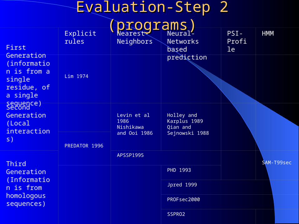
Evaluation-Step 2 (programs)Evaluation-Step 2 (programs)  Explicit rules Nearest-

NeighborsNeural-Networks based prediction

PSI-Profile

HMM

First Generation(information is from a single residue, of a single sequence)

Lim 1974        

Second Generation(Local interactions)

 Levin et al 1986Nishikawa and Ooi 1986

Holley and Karplus 1989Qian and Sejnowski 1988

   

PREDATOR 1996

Third Generation(Information is from homologous sequences)

APSSP1995

  SAM-T99sec

    PHD 1993

Jpred 1999

PROFsec2000

SSPRO2  

 

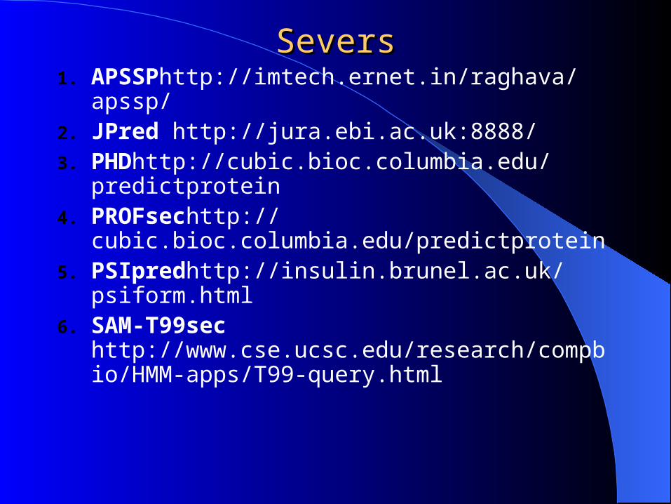
SeversSevers1. APSSPhttp://imtech.ernet.in/raghava/

apssp/2. JPred http://jura.ebi.ac.uk:8888/3. PHDhttp://cubic.bioc.columbia.edu/

predictprotein4. PROFsechttp://

cubic.bioc.columbia.edu/predictprotein5. PSIpredhttp://insulin.brunel.ac.uk/

psiform.html6. SAM-T99sec

http://www.cse.ucsc.edu/research/compbio/HMM-apps/T99-query.html

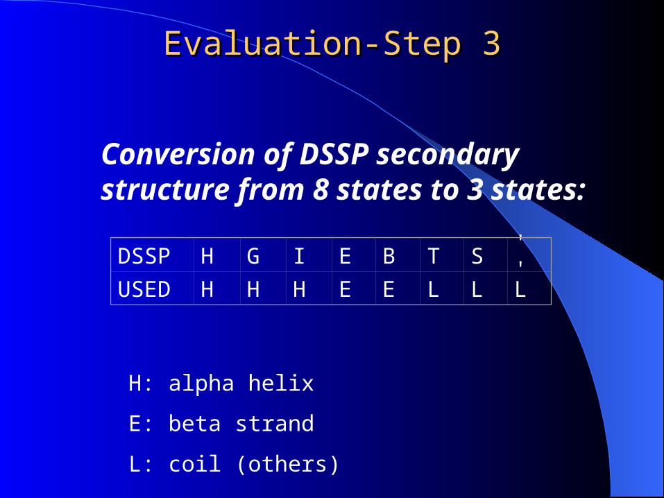
Evaluation-Step 3Evaluation-Step 3

Conversion of DSSP secondary structure from 8 states to 3 states:

DSSP H G I E B T S ' '

USED H H H E E L L L

H: alpha helix

E: beta strand

L: coil (others)

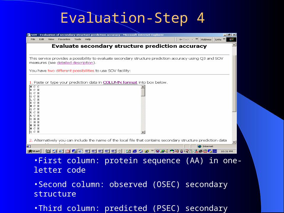
•First column: protein sequence (AA) in one-letter code

•Second column: observed (OSEC) secondary structure

•Third column: predicted (PSEC) secondary structure

http://predictioncenter.llnl.gov/local/sov/sov.html

Evaluation-Step 4

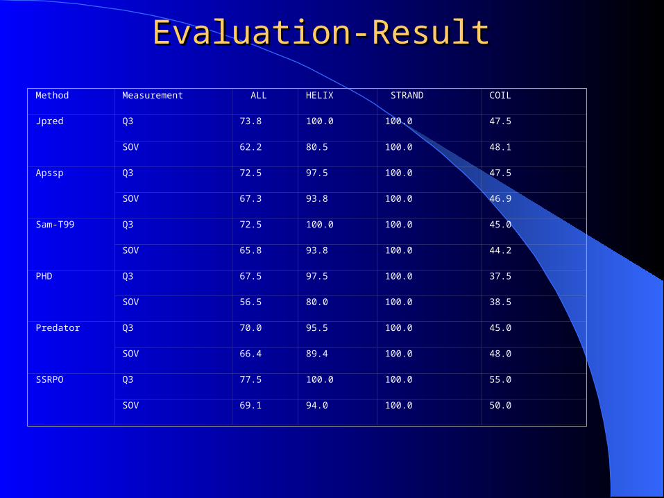
Evaluation-ResultEvaluation-Result

Method Measurement ALL HELIX STRAND COIL

Jpred Q3 73.8 100.0 100.0 47.5

SOV 62.2 80.5 100.0 48.1

Apssp Q3 72.5 97.5 100.0 47.5

SOV 67.3 93.8 100.0 46.9

Sam-T99 Q3 72.5 100.0 100.0 45.0

SOV 65.8 93.8 100.0 44.2

PHD Q3 67.5 97.5 100.0 37.5

SOV 56.5 80.0 100.0 38.5

Predator Q3 70.0 95.5 100.0 45.0

SOV 66.4 89.4 100.0 48.0

SSRPO Q3 77.5 100.0 100.0 55.0

SOV 69.1 94.0 100.0 50.0

 

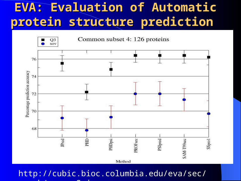
EVA: Evaluation of Automatic EVA: Evaluation of Automatic protein structure prediction protein structure prediction

http://cubic.bioc.columbia.edu/eva/sec/graph/common3.jpg

ConclusionConclusion

Jpred is the pioneer of methods which give high Q3 and SOV scores.

The 2ndary structure prediction using a jury of neural networks is one of the best methods.

REFERENCES1. Cuff JA, Clamp ME, Siddiqui AS, Finlay M, Barton GJ. “Jpred: A consensus secondary

structure prediction server,” Bioinformatics, 1998;14:892-893.

2. Cuff,J.A. and Barton, G.J. “Evaluation and improvement of multiple sequence methods for protein secondary structure prediction.” Proteins: Structure, Functions, and Genetics, 1999;34:508-519.

3. Cuff,J.A. and Barton, G.J. “Application of multiple sequence alignment profiles to improve protein secondary structure prediction.” Proteins: Structure, Functions, and Genetics, 2000;40:502-511.

4. Zemla et al. A modified definition of Sov, a Segment-Based Measure for Protein Secondary Structure Prediction Assessment. Protein; 1999:34:220-223

 5. Defay T, Cohen F. Evaluation of current techniques for ab initio protein structure

prediction. Proteins 1995; 23:431-445.  

6. Barton GJ. Protein secondary structure prediction. Curr Opin Struct Biol 1995; 5:372-376 

7. Schulz GE. A critical evaluation of methods for prediction of secondary structures. Ann Rev Biophys Chem 1988; 17:1-21

 8. Zhu Z-Y. A new approach to the evaluation of protein secondary structure predictions at

the level of the elements of secondary strucuter. Protein Eng 1995; 8:103-108