Embed Size (px)
Citation preview
PREDICTING STUDENT GRADUATION IN HIGHER EDUCATION USING
DATA MINING MODELS:
A COMPARISON
by
DHEERAJ RAJU
RANDALL SCHUMACKER, COMMITTEE CHAIR
JAMES MCLEAN
LORNE KUFFEL
BRIAN GRAY
MICHAEL CONERLY
A DISSERTATION
Submitted in partial fulfillment of the requirements
for the degree of Doctor of Philosophy
in the Department of Educational Studies
in Psychology, Research Methodology,
and Counseling in the Graduate School of
The University of Alabama
TUSCALOOSA, ALABAMA
2012

Copyright Dheeraj Raju 2012
ALL RIGHTS RESERVED

ii
ABSTRACT
Predictive modeling using data mining methods for early identification of students at risk
can be very beneficial in improving student graduation rates. The data driven decision planning
using data mining techniques is an innovative methodology that can be utilized by universities.
The goal of this research study was to compare data mining techniques in assessing student
graduation rates at The University of Alabama.
Data analyses were performed using two different datasets. The first dataset included pre-
college variables and the second dataset included pre-college variables along with college (end
of first semester) variables. Both pre-college and college datasets after performing a 10-fold
cross-validation indicated no difference in misclassification rates between logistic regression,
decision tree, neural network, and random forest models. The misclassification rate indicates the
error in predicting the actual number who graduated. The model misclassification rates for the
college dataset were around 7% lower than the model misclassification rates for the pre-college
dataset. The decision tree model was chosen as the best data mining model based on its
advantages over the other data mining models due to ease of interpretation and handling of
missing data.
Although pre-college variables provide good information about student graduation,
adding first semester information to pre-college variables provided better prediction of student
graduation. The decision tree model for the college dataset indicated first semester GPA, status,
earned hours, and high school GPA as the most important variables. Of the 22,099 students who

iii
were full-time, first time entering freshmen from 1995 to 2005, 7,293 did not graduate (33%).
Of the 7,293 who did not graduate, 2,845 students (39%) had first semester GPA < 2.25 with less
than 12 earned hours.
This study found that institutions can use historical high school pre-college information
and end of first semester data to build decision tree models that find significant variables which
predict student graduation. Students at risk can be predicted at the end of the first semester
instead of waiting until the end of the first year of school. The results from data mining analyses
can be used to develop intervention programs to help students succeed in college and graduate.

iv
DEDICATION
I would like to dedicate this study to my parents. I would also like to thank my family
and friends for supporting me during the course of this study. To my mother - So many years ago
your advice helped me begin this journey. To my dearest friends in Tuscaloosa – Thank you,
Words cannot express my gratitude.

v
LIST OF ABBREVIATIONS AND SYMBOLS
N Number of observations
π (x) Expected value of logistic regression
E(Y|x) Expected value of Y given x
β Model parameters
% Percentage
ε Error term
µ Mean
bag Bagged estimates
g(x) logit transformation
Estimated logit function
λ*
Wald statistic
∑ Summation
Wij Weights in neural network model
H0 Null Hypothesis
HA Alternative Hypothesis
Tanh Hyperbolic Tangent function
Tanh-1
Inverse Hyperbolic Tangent function
Log Logarithm
< Less than
= Equal to
vi
≠ Not equal to
> Greater than
≤ Less than or equal to
≥ Greater than or equal to
D Deviance statistic
SE Standard error of the coefficient estimate
ROC Receiver operating characteristics
UA University of Alabama
GPA Grade point average
AUC Area under curve
CHAID Chi-square automatic interaction detection
CART Classification and regression trees
VIF Variance inflation factor

vii
ACKNOWLEDGMENTS
I am grateful to my advisor and chair, Dr. Randall Schumacker, for everything he has
done for me over the course of my PhD and my life here at The University of Alabama. He has
been a great mentor, friend and family that has cheered me on during my successes and helped
me be the person I am. I would not be the same person without his supervision, Thank You Dr.
Schumacker.
I would like to thank Mr. Lorne Kuffel for his guidance, suggestions, and helpful
planning to take on a topic that I wanted to pursue. I am indebted to him for all his expert advice
on the topic and giving me an opportunity to get hands-on experience at the office of Institutional
Research. This would not have been possible without his supervision, Thank you Mr. Kuffel
I would like to thank Dr. James McLean for his guidance and support. He was the one
who encouraged me to enroll in this PhD program. Thank you, Dr. McLean.
I am extremely grateful to Dr. Brian Gray for his statistical guidance. He mentored me all
along this study and taught me everything I needed to learn. I thank him for taking the time to
meet with me whenever I needed any help. Thank you, Dr. Gray
I would like to thank Dr. Michael Conerly, for taking the time to serve on my committee
and supervise me. He has been my guiding light since my master’s program in statistics and also
my first teacher to teach me data mining. Thank you, Dr. Conerly

viii
CONTENTS
ABSTRACT ............................................................................................................ ………………ii
DEDICATION ............................................................................................................................... iv
LIST OF ABBREVIATIONS AND SYMBOLS ............................................................................v
ACKNOWLEDGMENTS ............................................................................................................ vii
LIST OF TABLES ....................................................................................................................... xiii
LIST OF FIGURES ..................................................................................................................... xvi
CHAPTER I: INTRODUCTION .....................................................................................................1
Problem Statement ...............................................................................................................1
Purpose of the Study ............................................................................................................4
Significance of the Study .....................................................................................................6
Limitations and Delimitations ..............................................................................................8
Definition of Terms..............................................................................................................9
Summary ............................................................................................................................10
CHAPTER II: REVIEW OF LITERATURE ................................................................................12
Student Graduation ............................................................................................................12
Data Mining Techniques ....................................................................................................24
Data Mining Applications in Higher Education ................................................................27
Enrollment..............................................................................................................28
Student Success and Graduation ............................................................................30
Research Questions ............................................................................................................37
ix
CHAPTER III: METHODS AND PROCEDURES .....................................................................38
Data Source ........................................................................................................................38
Assumptions ...........................................................................................................39
Sampling Technique ..............................................................................................40
Missing Values.......................................................................................................41
Variables ............................................................................................................................41
Research Design.................................................................................................................44
Research Procedure ............................................................................................................47
Software .................................................................................................................51
Model Comparison Techniques .............................................................................51
Receiver Operating Characteristics (ROC) .................................................51
Misclassification Rate .................................................................................54
Data Mining Models ..........................................................................................................56
Logistic Regression ................................................................................................56
Variable Selection Methods ........................................................................60
Multicollinearity ........................................................................................62
Decision Trees .......................................................................................................63
Pruning ........................................................................................................69
Random Forests .....................................................................................................69
Neural Networks ................................................................................................................72
Research Questions ............................................................................................................77
CHAPTER IV: RESULTS .............................................................................................................78
Exploratory Data Analysis .................................................................................................79
x
Graduation Rate by Freshmen Enrollment ............................................................79
Graduation Rate by Freshmen Gender…………………………………...………81
Graduation Rate by Ethnicity.................................................................................84
Graduation Rate by Home Distance ......................................................................86
Graduation Rate by Residency Status ....................................................................88
Graduation Rate by Enrollment Status ..................................................................89
Graduation Rate by First College Choice ..............................................................91
Graduation Rate by Work Information Choice ......................................................92
Graduation Rate by Advanced Placement Credit ..................................................94
Graduation Rate by High School Grade Point Average ........................................95
Graduation Rate by ACT score ..............................................................................97
Graduation Rate by First Semester GPA and Earned Hours .................................98
Summary…………………………………………………………………………99
Outliers and Missing Values ............................................................................................100
Research Question One ....................................................................................................101
Analyses of Pre-college Dataset ..........................................................................102
Forward Regression Results .....................................................................103
Backward Regression Results ...................................................................105
Stepwise Regression Results ....................................................................107
Neural Network Results .............................................................................109
Decision Tree Results ................................................................................114
Summary – Pre-College Dataset Analysis .................................................119
Misclassification Rates ...................................................................121

xi
Analyses of College Dataset ................................................................................122
Forward Regression Results .....................................................................123
Backward Regression Results ...................................................................125
Stepwise Regression Results ....................................................................128
Neural Network Results ............................................................................130
Decision Tree Results ...............................................................................135
Summary – College Dataset Analysis.......................................................141
Misclassification Rates ..................................................................141
Research Question Two ...................................................................................................142
Analyses of Pre-college Dataset ..........................................................................143
Decision Tree Results ...............................................................................144
Neural Network Results ............................................................................145
Random Forest Results .............................................................................146
Logistic Regression Results ......................................................................147
Summary – Pre-College Dataset Analysis……………………………....148
Analyses of College Dataset ................................................................................149
Decision Tree Results ...............................................................................152
Neural Network Results ...........................................................................153
Random Forest Results ............................................................................154
Logistic Regression Results .................................................................…155
Summary – College Dataset Analysis ………………………………….156
Research Question Three……………………………………………………………….156
CHAPTER V: SUMMARY, CONCLUSIONS, AND RECOMMENDATIONS.......................159
xii
Introduction ......................................................................................................................159
Summary of Findings .......................................................................................................160
Exploratory Data Analysis ...................................................................................160
Demographic Variables ............................................................................160
High School Variables ..............................................................................161
ACT Variables ..........................................................................................161
College Variables ......................................................................................162
Research Question One ........................................................................................162
Pre-College Dataset ..................................................................................162
College Dataset .........................................................................................163
Research Question Two ........................................................................................163
Pre-College Dataset ..................................................................................163
College Dataset .........................................................................................164
Research Question Three .....................................................................................164
Conclusions ......................................................................................................................164
Practical Application ........................................................................................................166
Recommendations ............................................................................................................170
REFERENCES ............................................................................................................................173
APPENDICES .............................................................................................................................182
xiii
LIST OF TABLES
3.1 List of Variables ....................................................................................................................44
3.2 ROC Table ............................................................................................................................54
3.3 Misclassification Table .........................................................................................................55
4.1 Variables in Datasets.............................................................................................................78
4.2 Graduation Rates for First-time Freshmen by Enrollment Year ...........................................79
4.3 Graduation Rate for First-time Freshmen by Gender ...........................................................81
4.4 Graduation Rate for First-time Freshmen by Ethnicity ........................................................83
4.5 Graduation Rate for First-time Freshmen by Distance from Home .....................................86
4.6 Graduation Rate by Residency Status ...................................................................................88
4.7 Graduation Rate for First-time Freshmen by Enrollment Status ..........................................89
4.8 Graduation Rate for First-time Freshmen by First College Choice ......................................91
4.9 Graduation Rate for First-time Freshmen by Work Information ..........................................92
4.10 Graduation Rate for First-time Freshmen by Advanced Placement Credit ..........................94
4.11 Graduation Rate for First-time Freshmen by High School English GPA .............................95
4.12 Graduation Rate for First-time Freshmen by ACT score ......................................................97
4.13 Graduation Rate for Freshmen by First Semester GPA and Earned Hours ..........................98
4.14 Forward Selection Regression Significant Variables .........................................................104
4.15 Forward Selection Regression Misclassification Table ......................................................104
4.16 Backward Selection Logistic Regression Significant Variables .........................................106
4.17 Backward Selection Regression Misclassification Table ...................................................106
xiv
4.18 Stepwise Selection Logistic Regression Significant Variables ..........................................108
4.19 Stepwise Selection Misclassification Table ........................................................................108
4.20 Neural Network Optimization Results ................................................................................112
4.21 Neural Network Model Misclassification Table .................................................................113
4.22 Decision Tree Variable Importance Output ........................................................................118
4.23 Decision Tree Model Misclassification Table ....................................................................118
4.24 Area Under Curve (AUC) Values for Five Models ............................................................121
4.25 Misclassification Rates for Five Models.............................................................................121
4.26 Forward Selection Regression Significant Variables .........................................................124
4.27 Forward Selection Misclassification Table .........................................................................124
4.28 Backward Selection Logistic Regression Significant Variables .........................................126
4.29 Backward Selection Misclassification Table ......................................................................127
4.30 Stepwise Selection Logistic Regression Significant Variables ..........................................129
4.31 Stepwise Selection Misclassification Table ........................................................................130
4.32 Neural Network Optimization Results ................................................................................133
4.33 Neural Network Model Misclassification Table .................................................................134
4.34 Decision Tree Variable Importance Output ........................................................................138
4.35 Decision Tree Model Misclassification Table ....................................................................138
4.36 Area Under Curve (AUC) Values for Five Models ............................................................141
4.37 Misclassification Rates for Five Models.............................................................................141
4.38 Decision Tree Model Results ..............................................................................................144
4.39 Neural Network Model Results ..........................................................................................145
4.40 Neural Network Model Results ..........................................................................................146
xv
4.41 Logistic Regression Model Results ....................................................................................147
4.42 Misclassification Rates for Four Models ............................................................................148
4.43 Decision Tree Model Results ..............................................................................................152
4.44 Neural Network Model Results ..........................................................................................153
4.45 Random Forests Model Results ..........................................................................................154
4.46 Logistic Regression Model Results ....................................................................................155
4.47 Misclassification Rates for Four Models ............................................................................156
4.48 Graduation Rates in Terms of First-semester GPA and Earned Hours ..............................157
4.49 High School GPA for Leaving Students with First-semester GPA less than 2.99
and less than 12 Earned Hours ............................................................................................158
4.50 Advanced Placement Credit for Leaving Students with First-semester GPA less than
2.99 and less than 12 Earned Hours ...................................................................................158
5.1 Misclassification Rates for Pre-college and College Datasets ............................................164
5.2 High School GPA Breakdown for Graduated First-time Freshmen ..................................166
5.3 First-Semester GPA Breakdown for Graduated First-time Freshmen ...............................168
5.4 First-semester Earned Hours for Graduated First-time Freshmen .....................................169

xvi
LIST OF FIGURES
1.1 BA Degree Completion Rates from 1880 to 1980 ..................................................................2
1.2 Percentage of four-year college students who earn a degree within five years of entry ........3
1.3 Percentage of first year students at four-year colleges who return for second year. ..............4
2.1 Tinto’s (1975) Theoretical Model of College Withdrawal ...................................................16
2.2 Tinto’s 13 Primary Propositions ...........................................................................................18
2.3 Bean’s Student Attrition Model ............................................................................................20
2.4 Relationship between Data Mining and Knowledge Discovery ...........................................26
3.1 Phases of the CRISP-DM Process ........................................................................................47
3.2 Example ROC Curve ............................................................................................................54
3.3 A Simple Decision Tree ........................................................................................................65
3.4 Example Decision Tree .........................................................................................................66
3.5 Simple Neural Network ........................................................................................................72
3.6 Neural Networks Architecture ..............................................................................................73
3.7 Example Feed-Forward Neural Networks ............................................................................74
4.1 Overall First-time Freshmen Graduation Rate by Year ........................................................80
4.2 Outlier Analysis JMP Output ..............................................................................................101
4.3. SAS® Enterprise Miner Data Analysis Diagram ...............................................................102
4.4. Enterprise Miner Forward Regression Options ..................................................................103
4.5. Enterprise Miner Backward Regression Options ................................................................105
4.6. SAS® Enterprise Miner Stepwise Regression Options ......................................................107

xvii
4.7. SAS® Enterprise Miner Neural Networks Options ............................................................109
4.8. SAS® Enterprise Miner Neural Network Network Options ..............................................110
4.9. SAS® Enterprise Miner Neural Network Optimization Options .......................................110
4.10 SAS® Enterprise Miner Decision Tree Options Screenshot ..............................................114
4.11 Decision Tree Model...........................................................................................................116
4.12 SAS® Enterprise Miner Model Comparison Option Screenshot ......................................119
4.13 SAS® Enterprise Miner ROC Curve Screenshot ...............................................................120
4.14 SAS® Enterprise Miner Data Analysis Diagram ...............................................................122
4.15 Enterprise Miner Forward Regression Options ..................................................................123
4.16 Enterprise Miner Backward Regression Options ................................................................125
4.17 SAS® Enterprise Miner Stepwise Regression Options ......................................................128
4.18 SAS® Enterprise Miner Neural Networks Options ............................................................130
4.19 SAS® Enterprise Miner Neural Network Network Options ..............................................131
4.20 SAS® Enterprise Miner Neural Network Optimization Options .......................................132
4.21 SAS® Enterprise Miner Decision Tree Options Screenshot ..............................................135
4.22 Decision Tree Model...........................................................................................................136
4.23 SAS® Enterprise Miner Model comparison Option Screenshot .......................................139
4.24 SAS® Enterprise Miner ROC Curve Screenshot ...............................................................140
4.25 R Data Summary Snapshot .................................................................................................143
4.26 Data Summary After Stratification Sampling Snapshot .....................................................144
4.27 R Data Summary Snapshot .................................................................................................150
4.28 Data Summary After Stratification Sampling Snapshot ......................................................151
5.1 High School GPA Breakdown for Graduated First-time Freshmen ...................................167

xviii
5.2 First-semester GPA Breakdown for Graduated First-time Freshmen .................................168
5.3 First-semester Earned Hours for Graduated First-time Freshmen .....................................170

1
CHAPTER I:
INTRODUCTION
Problem Statement
High school graduates enroll in colleges to earn a college degree; however, some students
do not graduate. An institution fails to retain its student if the student does not graduate from
where they started. Seidman (2005) defines student retention as the “ability of a particular
college or university to successfully graduate the students that initially enroll at that institution”
(p.3). Most freshmen are not prepared to make a successful shift from high school to college and
also may be underprepared to face several challenges in college transition, which can be very
stressful (Lu, 1994). Universities with high leaver rates go through loss of fees, tuition, and
potential alumni contributors (DeBerrad, Spielmans, & Julka, 2004). Federal and state
governments across the United States realize the importance of higher education in achieving a
better economy and have been offering several programs for all kinds of students to improve
graduation. Also, universities have developed several intervention programs to reduce the
number of leavers (Siedman, 2005). Regardless of these intensive efforts to improve student
graduation, leaver rates are high across the United States (Yu, DiGangi, Jannasch-Pennell, &
Kaprolet, 2010). The U.S. Department of Education’s Center for Educational Statistics reported
that only 50% of those who enroll in college earn a degree (Siedman, 2005). Noel and Levitz
(2004) indicated that both private and public institutions have experienced escalating challenges
associated with enrollment related issues in recent years. Student graduation is a very important
display of academic performance and enrollment management to any university.
2
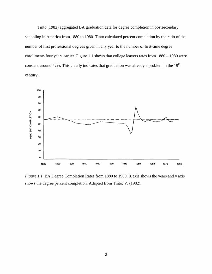
Tinto (1982) aggregated BA graduation data for degree completion in postsecondary
schooling in America from 1880 to 1980. Tinto calculated percent completion by the ratio of the
number of first professional degrees given in any year to the number of first-time degree
enrollments four years earlier. Figure 1.1 shows that college leavers rates from 1880 – 1980 were
constant around 52%. This clearly indicates that graduation was already a problem in the 19th
century.
Figure 1.1. BA Degree Completion Rates from 1880 to 1980. X axis shows the years and y axis
shows the degree percent completion. Adapted from Tinto, V. (1982).
3
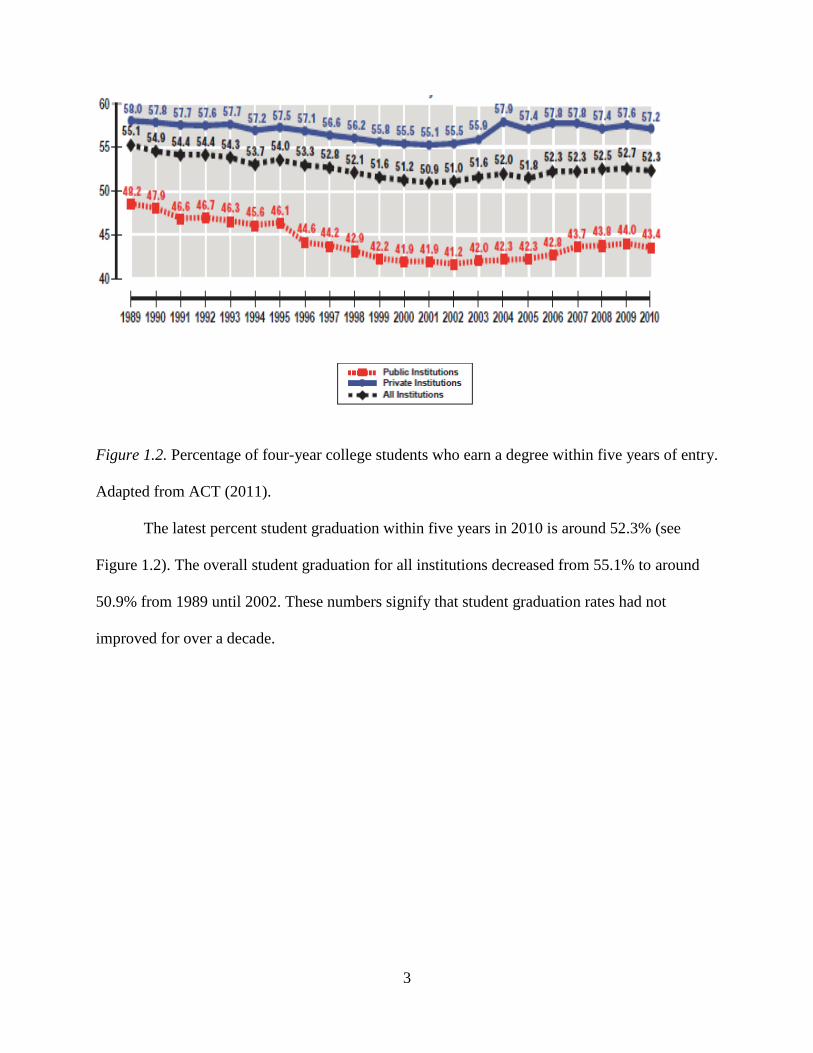
Figure 1.2. Percentage of four-year college students who earn a degree within five years of entry.
Adapted from ACT (2011).
The latest percent student graduation within five years in 2010 is around 52.3% (see
Figure 1.2). The overall student graduation for all institutions decreased from 55.1% to around
50.9% from 1989 until 2002. These numbers signify that student graduation rates had not
improved for over a decade.
4
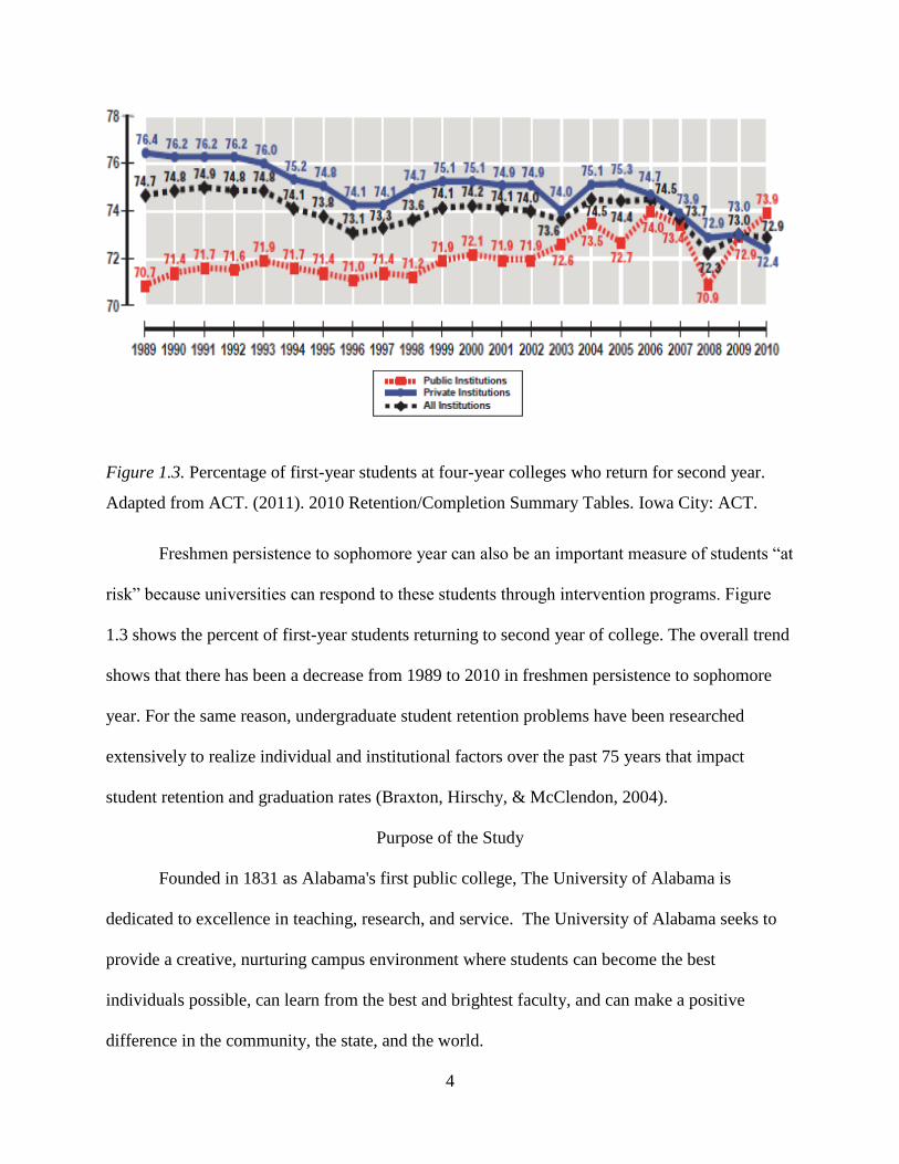
Figure 1.3. Percentage of first-year students at four-year colleges who return for second year.
Adapted from ACT. (2011). 2010 Retention/Completion Summary Tables. Iowa City: ACT.
Freshmen persistence to sophomore year can also be an important measure of students “at
risk” because universities can respond to these students through intervention programs. Figure
1.3 shows the percent of first-year students returning to second year of college. The overall trend
shows that there has been a decrease from 1989 to 2010 in freshmen persistence to sophomore
year. For the same reason, undergraduate student retention problems have been researched
extensively to realize individual and institutional factors over the past 75 years that impact
student retention and graduation rates (Braxton, Hirschy, & McClendon, 2004).
Purpose of the Study
Founded in 1831 as Alabama's first public college, The University of Alabama is
dedicated to excellence in teaching, research, and service. The University of Alabama seeks to
provide a creative, nurturing campus environment where students can become the best
individuals possible, can learn from the best and brightest faculty, and can make a positive
difference in the community, the state, and the world.
5
One of the current concerns for the university and its administration is the growth of the
student population. Although the President of the university has set an aggressive goal for
enrollment growth, there is still an underlying student graduation focus that the university is
keeping in mind. That focus involves the ability of each student enrolled at the university to
receive optimal educational opportunities and tools, leading to student graduation. An
institutions quality is assessed by its national ranking that consists of some factors like students
with best grades, scholarships, students who do not leave and students who graduate.
With a record student enrollment of 30,232 in the fall 2010, The University of Alabama
continues to be the state’s largest university. Enrollment increased by 1,425 students, or about
5%, over fall 2009. Enrollment at UA is up 48% since fall 2002. The graduation rate at The
University of Alabama remains at around 65%, which means that about 35% of entering
Freshmen do not graduate.
The key to effectively understanding this complex balance between enrollment and
graduation is in the application of optimization algorithms or procedures such as data mining and
predictive modeling. Admissions personnel and management must be able to predict future
criteria for a student who graduates or who does not graduate and be able to help students who
will not graduate. Having such accurate predictions will greatly aid in the ability of the
administration of a university to keep this positive balance between growth, quality, retention,
and graduation.
Understanding student success behavior is an essential focus of institutional researchers
at The University of Alabama. Institutional managers are always interested in answers to certain
questions: why do students not graduate? Why do students transfer to another university? Why
do some students graduate before others? Why do some students take longer than other students
6
to graduate? Who are the students at risk? Answers to these questions will help enrollment
managers to take appropriate measures to improve enrollment and graduation rates, e.g. develop
effective intervention programs.
The purpose of this research study is to compare different data mining techniques as
predictive models of student graduation at The University of Alabama. This research will build
and compare the statistical predictive data mining models like logistic regression with four
different variable selection methods, decision tree, random forests and neural networks. Each of
these models will be optimized to fit the student retention data and then evaluated to determine
the best data mining model. This research study will also find important characteristics of
students who graduate versus students who do not graduate. Finally, this study will contribute to
the meager research in effectiveness of data mining techniques applied in higher education and
also help educational institutions better use data mining techniques to inform student graduation
strategies.
Significance of Study
Family conditions and better transition from high school to college are important factors
that help students graduate. Research studies show that early identification of leaver students and
intervention programs are key aspects that can lead to student graduation. Boyer (2001) argued
that a good institution should be able to hold on to its students even if it requires as much effort
as it does at getting them to campus. One of the major concerns for institutional managers is the
capability to predict potential student leavers. Predictive modeling for early identification of
students at risk could be very beneficial in improving student graduation. Predictive models use
data stored in institution databases that consist of student’s financial, demographical, and
academic information. Predictive data mining therefore use large datasets to analyze student

7
graduation problems. The predictive data mining decision planning is an innovative methodology
that should be employed by universities.
Research suggests some important data associated with four-year degree completion
(Cabrera, Burkum, & La Nasa, 2005). They include the following:
1. Background characteristics;
2. Support in high school;
3. College planning;
4. Degree ambition;
5. College path;
6. Academic involvement;
7. College experiences and curriculum;
8. Financial aid; and
9. Parental conscientiousness.
Braxton et al. (1997) suggested that understanding this type of data that leads to student
leavers is a complicated problem, even though there is plenty of research implying some
common variables related to student graduation. The complexity of understanding factors
affecting student graduation at over 3,600 universities in the United States is due to differences
in location, student demographics, and funding.
Most research-based data mining applications in higher education consider retention from
freshmen to sophomore year. There have also been research studies on predicting enrollment,
where statistical models have been used to predict the enrollment size or student acceptance.
Herzog (2006) used decision trees and neural networks to compare it with regression in
estimating student retention and degree completion time. Herzog used sophomore year data for
8
retention analysis. Sujitparapitaya (2006) observed significant predictors that influence decisions
of first-time freshmen on their first-year completion. Ho Yu et al. (2010) used data mining
techniques for identifying predictors of student retention from sophomore to junior year. Prior
research has used neural networks, classification tress, and multivariate adaptive regression
splines (MARS) to predict student characteristics. Nara et al. (2005) suggested a major gap in
literature on retaining students past their Freshmen year. Although freshmen to sophomore year
or sophomore to senior year is an important indicator of student success towards graduation, this
year alone does not completely explain student graduation success. Therefore, it is important to
identify associated variables from freshmen year leading to student graduation. This research
will consider student graduation as student success rather than completion of any transition year.
This study also used an ensemble classifier data mining technique called random forests that
consists of many decision trees. Random forests have a very high accuracy in large datasets
(Breiman, 2001), which has been hardly used in higher education data mining research. The
significance of this study is in the comparison of several data mining techniques and their
classification accuracy using important indicator variables of student graduation.
Limitations and Delimitations
Results of this research study are applicable only to the University of Alabama and
cannot be generalized to any other universities in the United States. Nevertheless, the statistical
data mining techniques used in this research can be applicable to other universities in analyzing
their respective student graduation data and in the field of higher education institutional research.
The data for this study was delimited to first-time Freshmen students from 1995 to 2005. This
research study will also be delimited to student graduation within six years from their initial
student enrollment.
9
Definition of Terms
At risk students. At risk students are defined as students who have a higher probability of
not graduating from the institution.
Attribute. An attribute in this research is referred to as a single variable, such as race or
gender. Attributes are used to build statistical models. Variable is another equivalent term for
attribute.
Cohort. Cohort refers to a group of students who have shared a particular time. For
example, freshmen students entering fall 2010 are considered to be 2010 cohort students.
Data. Oxford dictionary’s definition of data as “facts and statistics collected together for
reference and analysis” will be used in this research.
Data Mining. Frawley et al. (1991) defined data mining as the non trivial extraction of
implicit, previously unknown, and potentially useful information from data.
Decision Trees. Decision trees are ordered as a sequence of simple questions. The
answers to these simple questions conclude what might be the next question. The decision
outcomes result in a network of links that forms a tree-like structure.
Graduation. Graduation is defined as a first-time entering Freshmen student who
eventually graduates within six years of enrollment.
Leavers. Left school for any number of reasons, financial, grades, hardship, etc.
Logistic Regression. Logistic regression is a predictive modeling technique that finds an
association between the independent variables and the logarithm of the odds of a categorical
response variable.
Modeling. Modeling in this study refers to the act of building equations that use observed
data in order to predict future instances with future unobserved data.

10
Neural Networks. Artificial neural network models are learning algorithms that analyze
any given classification problem. Interconnected “neurons” help in all mathematical operations
in transforming inputs to outputs (Abu-Mostafa, 1996).
Random Forests. Random forests is a predictive modeling algorithm that builds a series
of de-correlated decision trees and then averages them. An Ensemble decision tree model is built
based on multi classifier’s decision.
Retention. Retention is referred to as first-time student freshmen who gradually progress
and graduate within six years of enrollment.
Student success. Student success is defined based on student graduation. A successful
student gradually progresses through his/her degree and eventually graduates within six years of
enrollment.
Variable. Variable is defined as the characteristic or attribute of a student. For example,
gender, age, and GPA are variables.
Misclassification Rates. The misclassification rate indicates the error in predicting the
actual number who graduated.
Receiver Operating Characteristics (ROC). ROC curve illustrates a graphical display that
evaluates the forecasting precision of a predictive model.
Summary
The purpose of this research study is to compare data mining techniques in analysis of
student variables leading to student graduation at The University of Alabama. This study will
contribute to the meager research in effectiveness of data mining techniques applied in higher
education and also help educational institutions better use data mining techniques to inform
student graduation strategies. From an institutions perspective, enhanced student retention

11
leading to graduation improves enrollment management, cuts down on recruiting costs, and also
improves the university standing. From a student’s perspective, student retention leading to
graduation has societal, personal and economic implications.
12
CHAPTER II:
REVIEW OF LITERATURE
Student Graduation
Literature defines student graduation or student success in terms of retention rates.
Hagedorn (2005) defines retention rate as first-time Freshmen students who graduate within six
years of their original enrollment date. Druzdel and Glymour (1999) define “student retention
rate” as the percent of entering Freshmen who eventually graduate from the university where
they enrolled as a Freshmen. Kramer (2007) suggested an uncomplicated definition of retention
as an “individual who enrolls in college and remains enrolled until the completion of a degree.”
Freshmen persistence is usually defined in terms of returning students who re-enroll after their
first-year for the sophomore semester (Mallinckrodt & Sedlacek, 1987).
Student retention leading to graduation has been extensively researched in higher
education over the past thirty years. The earliest student success studies in higher education dates
back to the 1930s. These early studies were referred to as student mortality. A large student
leaver’s problem became a widespread concern among colleges throughout the Unites States in
the 1970s. As a result, there was a number of student success theories published at this time
which later lead to further research, currently resulting in thousands of studies (Seidman, 2005).
Seidman (2005) summarized some of the important theory related concepts discussed in student
graduation research over the years. They include
1. Attrition: Students who do not register in successive semesters;
2. Dropout: Students who did not complete their degree;

13
3. Dismissal: Students who were not authorized to enroll by the school;
4. Mortality: Students who did not persist until graduation;
5. Persistence: Students who stay in college and complete their degree;
6. Retention: Capability of the college to retain a student until graduation;
7. Stopout: Students who briefly depart from a college; and
8. Withdrawal: Students who exit from a college.
Most of the early student success studies concentrated on psychological approaches and
demographic attributes that tried to analyze student patterns in attrition. Psychological analysis
included personality characteristics like motivation, maturity, and temperament as some of the
causes for students to stay in college to complete their degree (Summerskill, 1962). Summerskill
published one of the earliest studies that analyzed college student departure where he reported
student retention statistics from the first half of the 20th
century. Spady, in 1971, published one of
the earliest longitudinal data analyses completed at the University of Chicago which explained
the undergraduate student leaving process. Spady noted that there were six key types of studies
published from the 1950s to 1960s. They include the following:
1. Philosophical studies: Theoretical studies frequently dealing with dropouts in
college and avoiding attrition;
2. Autopsy: Studies accounted for information on causes of student dropout;
3. Census: Studies tried to illustrate dropouts and attrition within and across schools;
4. Case studies: Case studies followed students recognized as potential dropouts to
verify their success/failure to graduate from college;
5. Descriptive: Descriptive studies presented attributes of students who dropped out;
and

14
6. Predictive: Predictive studies tried to recognize some of the admissions criteria
that could be used to predict student success.
Durkheim (1961) proposed the theory of suicide to elucidate student attrition. He found
that people committed suicide because they could not integrate with the social system. His theory
explained that egotistical suicide could happen with individuals if they became secluded from
communities because of inability to institute association. The model discussed two different
types of association. The first form was the social associations, which took place through
interaction with other people in the society which led to a development of social connections.
The second form was the intellectual associations, which took place where there was universal
agreement in values and beliefs.
Spady (1971) employed the suicide theory where he saw a similarity between people
committing suicide and people dropping out of school. In both cases people left the social
system. His model accentuated the communication between individual student attributes and
some of the key aspects of college atmosphere. The sociological model explained student
departure or leaving relating to interaction between student and the social (college) environment.
This model emphasized that some of the student attributes such as values, interest, ability, and
attitudes are exposed to college atmosphere like faculty, classrooms, and peers. Any student is
more likely to drop out of college if the college environment is not harmonious with student
attributes.
Furthermore, around the 1970s, institutions were facing extreme enrollment shortages
because the population of 18-year olds was dropping. Educational experts predicted that about
30% of colleges would have to close (Harrington & Sum, 1988). Ironically, enrollments actually

15
increased twice the prediction because of developing new markets, improving retention rates and
attending new students.
Tinto (1975) developed Spady’s theory by concentrating more on the interactions
between academic and social systems of higher education. Tinto’s student integration model is
one of the finest and frequently cited theories in student retention (Seidman, 2005). Tinto’s
Interactionlist theory highlighted that fact that there was a very strong positive relationship with
student’s level of academic and social integration and their persistence in college. In other words,
students with higher levels of academic and social integration were believed to persist in college
and graduate. Tinto’s model identified some relationship between before entry college
characteristics, institutional incidents, institutional and social integration with goals and
outcomes. Pre-college entry characteristics included family background, abilities, and former
schooling, etc. Institutional incidents included faculty interactions, on campus activities, and peer
interactions. Goals and outcomes included institutional commitment and departure respectively
(Tinto, 1987). Figure 2.1 shows Tinto’s theoretical model. In summary there were five elements
in Tinto’s theoretical model. They include
1. Individual Characteristics: Included family background characteristics, socio-
economic status, academic ability, race and gender;
2. Pre-college schooling: Characteristics of student’s secondary school, high school
and social attachments;
3. Academic integration: Included structural and normative dimensions. Structural
dimensions included meeting standards of college and normative dimension
included students identification with the structure of academic system;

16
4. Social integration: Amount of equivalence between student and the social system
of a college; and
5. Commitments: included goal to stay and graduate.
Figure 2.1. Tinto’s (1975) Theoretical Model of College Withdrawal. Adapted from Tinto, V.
(1975). Leavers from higher education: A theoretical synthesis of the recent research. A Review
of Educational Research, 45, 89-125.
Braxton et al. (1997) summarized Tinto’s model into 15 testable propositions. They are
as follows:
1. The intensity of preliminary commitment to the college can be directly related to
a student's entrance attributes;
2. A student's entrance attributes can affect their commitment towards the goal of
graduation from college;
3. A student's level of perseverance and determination in their studies can be
reflective of their entrance attributes;
4. A preliminary commitment to the goal of graduation can affect a student's level of
integration into academia;
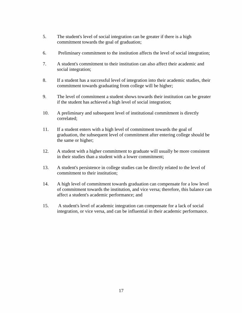
17
5. The student's level of social integration can be greater if there is a high
commitment towards the goal of graduation;
6. Preliminary commitment to the institution affects the level of social integration;
7. A student's commitment to their institution can also affect their academic and
social integration;
8. If a student has a successful level of integration into their academic studies, their
commitment towards graduating from college will be higher;
9. The level of commitment a student shows towards their institution can be greater
if the student has achieved a high level of social integration;
10. A preliminary and subsequent level of institutional commitment is directly
correlated;
11. If a student enters with a high level of commitment towards the goal of
graduation, the subsequent level of commitment after entering college should be
the same or higher;
12. A student with a higher commitment to graduate will usually be more consistent
in their studies than a student with a lower commitment;
13. A student's persistence in college studies can be directly related to the level of
commitment to their institution;
14. A high level of commitment towards graduation can compensate for a low level
of commitment towards the institution, and vice versa; therefore, this balance can
affect a student's academic performance; and
15. A student's level of academic integration can compensate for a lack of social
integration, or vice versa, and can be influential in their academic performance.
18
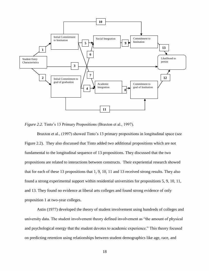
Figure 2.2. Tinto’s 13 Primary Propositions (Braxton et al., 1997).
Braxton et al., (1997) showed Tinto’s 13 primary propositions in longitudinal space (see
Figure 2.2). They also discussed that Tinto added two additional propositions which are not
fundamental to the longitudinal sequence of 13 propositions. They discussed that the two
propositions are related to interactions between constructs. Their experiential research showed
that for each of these 13 propositions that 1, 9, 10, 11 and 13 received strong results. They also
found a strong experimental support within residential universities for propositions 5, 9, 10, 11,
and 13. They found no evidence at liberal arts colleges and found strong evidence of only
proposition 1 at two-year colleges.
Astin (1977) developed the theory of student involvement using hundreds of colleges and
university data. The student involvement theory defined involvement as “the amount of physical
and psychological energy that the student devotes to academic experience.” This theory focused
on predicting retention using relationships between student demographics like age, race, and
Student Entry
Characteristics
Initial Commitment
to Institution
Initial Commitment to
goal of graduation
Social Integration
Academic
Integration
Commitment to
Institution
Commitment to
goal of Institution
Likelihood to
persist
1
2
5
6
7
4 8
13
12
9
10
11
3

19
gender, etc., and institutional characteristics like location, size with the level of academic and
social involvement (Astin, 1977; Astin 1985). Astin (1985) explained that student involvement
refers to student behaviors, implying student actions rather than student’s thoughts. The theory of
student involvement can be summarized into the five following postulates:
1. “Involvement refers to the investment of physical and psychological energy in
various objects.” An object can refer to any student experience activities or tasks;
2. “Regardless of the object, involvement occurs along a continuum.” Diverse
students devote more energy than other students;
3. “Involvement has both quantitative and qualitative features”. Quantitative features
of involvement comprises of amount of time devoted to any activity. Qualitative
features of involvement might include severity of approach with which the object
is dealt;
4. “The amount of student learning and personal development associated with any
educational program is directly proportional to the quality and quantity of student
involvement in that program;”
5. “The effectiveness of any educational policy or practice is directly related to the
capacity of the policy or practice to increase student involvement.”
Astin argued that students who actively engaged in their social environment had better
learning/growth and educators needed to create more prospects for in and out of classroom
involvement.
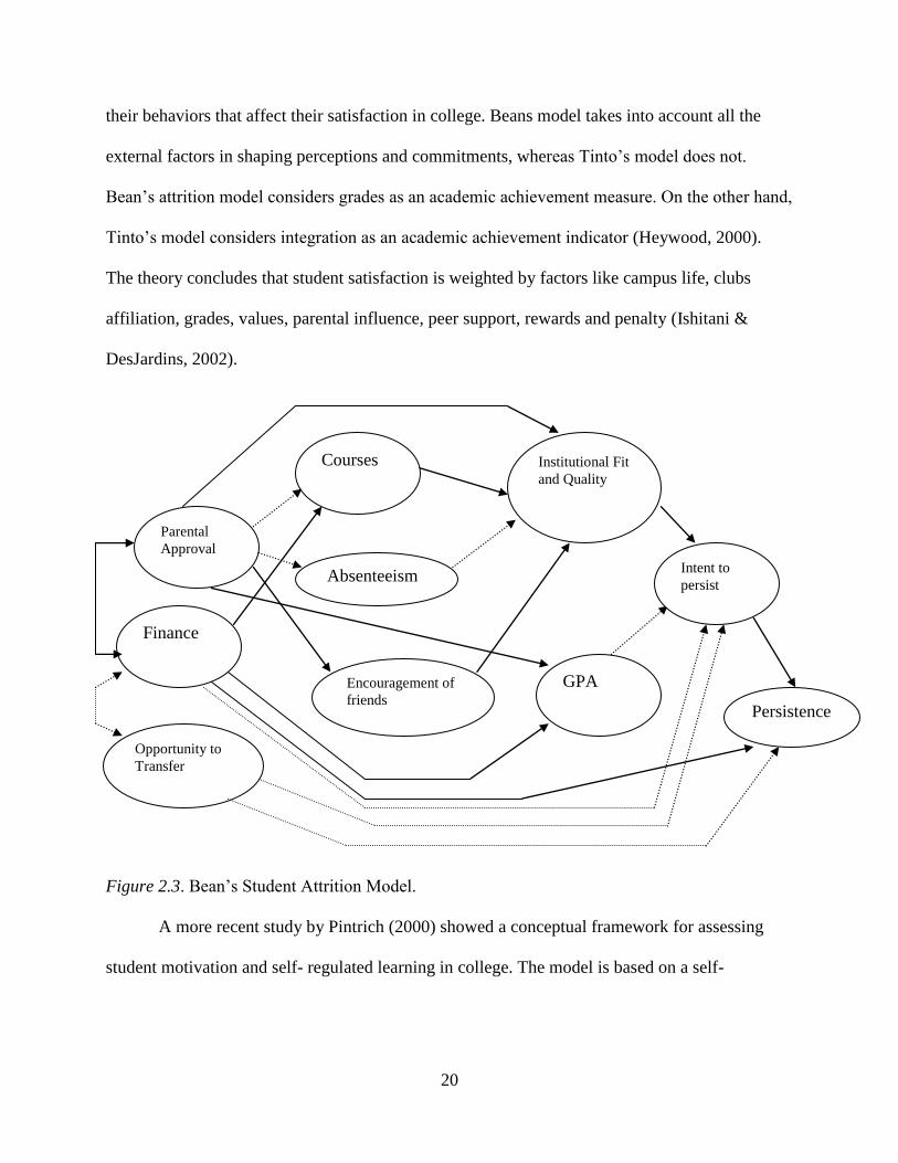
Bean (1980) developed the student attrition model (see Figure 2.3). The student attrition
model stresses the fact that a student’s experience at their college plays a big role in their
decision to stay or leave. This model is based on the communications of student attitudes and
20
their behaviors that affect their satisfaction in college. Beans model takes into account all the
external factors in shaping perceptions and commitments, whereas Tinto’s model does not.
Bean’s attrition model considers grades as an academic achievement measure. On the other hand,
Tinto’s model considers integration as an academic achievement indicator (Heywood, 2000).
The theory concludes that student satisfaction is weighted by factors like campus life, clubs
affiliation, grades, values, parental influence, peer support, rewards and penalty (Ishitani &
DesJardins, 2002).
Figure 2.3. Bean’s Student Attrition Model.
A more recent study by Pintrich (2000) showed a conceptual framework for assessing
student motivation and self- regulated learning in college. The model is based on a self-
Institutional Fit
and Quality
Finance
Opportunity to
Transfer
Courses
Absenteeism
Encouragement of
friends
Parental
Approval
GPA
Intent to
persist
Persistence
21
regulatory (SRL) perspective on student motivation and learning. The assumptions related to the
SRL model are as follows:
1. “The active, constructive assumption” – Learners are dynamic constructive
participants;
2. “The potential for control assumption” – Learners can monitor, control and
regulate certain aspects in their own cognition, motivation, and behavior;
3. “The goal, criterion, or standard assumption” – There is some criterion by which
to determine whether the learning process should continue or if some type of
change is necessary; and
4. “The mediation assumption” – Learners activities are mediators between personal
characteristics and authentic performance.
Twenty-first century ended with student retention efforts well established at universities
across the Unites States. There has been several thousands of research studies published on
student retention leading to graduation. A journal, Journal of College Retention: Research,
Theory and Practice, was created to disseminate these research findings.
There have also been numerous studies supporting academic ability as an exceedingly
important variable leading to student graduation. A student graduation research study from a
vocational study program at the Woodrow Wilson Rehabilitation Center found that prior
education is a good predictor of student graduation (Reason, 2003).. Variables like college
admission test scores, high school grade point average, race and gender are regularly used as
important retention predictors leading to graduation .A study at the Terry campus of Delaware
Technical and community college showed that students who lacked academic ability were most

22
likely to drop out of college (Falatek, 1993). College GPA was also a significant variable that
related to leavers past their first-year, which impacted student graduation rates.
Summers (2000) identified some other variables like socio-economic status, employment
status, motivation, social integration, satisfaction, parent’s education level, dedication,
interaction with faculty, and age, etc to be significant contributors to graduation rates. Some of
these variables agreed with Tinto’s and Astin’s theories.
Student ethnicity is also shown to be an extremely significant factor in student retention
leading to graduation. University of Milwaukee saw white students graduating at significantly
higher rates than other races (Boykin, 1983). University of Southwestern Louisiana saw white
students graduating at a higher rate than African American students (Dial, 1987). A longitudinal
survey of more than 50,000 students from 1965-2001 conducted by the National Center of
Educational Statistics (NCES) revealed that African American and Hispanic students had lower
graduation rates than Asian and Caucasian. While African American and Hispanic survey
responses were combined, the study showed a completion rate of 47% when compared to Asian
and Caucasians with a completion rate of 67% (Berkner, He, & Cataldi, 2002). Other variables
related academic goal such as cumulative grade point average, credit hours attempted, academic
standing situation, and how students enrolled were found to be good predictors of graduation.
Cumulative hours taken in the first year of college was found to be a significant predictor of
college student’s persistence from Freshmen to sophomore year (Kiser & Price, 2008), which
would lead to student success or graduation.
The primary cause of students leaving college (not graduating) is because of financial
difficulty (ACT, 2010). Financial status situation in terms of tuition grants, student loans, work
study, and all costs related to college plays a very significant role in college retention (Wetzel,
23
O'Toole, & Peterson, 199). A survey given to friends of students who dropped out of college
revealed three primary issues such as financial problems, academic problems and clashing
schedules to be some of the causes for student leaving (Mayo, Helms, & Codjoe, 2004).
Financial aid has been a very important factor in helping students graduate. Students with
some kind of financial aid graduated at higher rates than those who did not receive financial aid.
Students with financial aid graduated in higher rates with a baccalaureate degree within a six
year graduation period than students with no financial aid (Walsh, 1997). Students with higher
socio economic status graduated in higher numbers than students with lower socio economic
status.
Walsh (1997) also reported that the past 50 years of studies in student retention identified socio
economic status to be a very important factor in graduation rates.
High school GPA was found to have a significant correlation with persistence. All though
high school GPA was found to be correlated with retention it was not a good predictor (Seidman,
2005). Additionally, a national research study with a sample of nearly 20,000 first-year students
on how student experiences and campus programs affect key academic outcomes of the first
year, showed that pre-college grades and ‘perceptions of academic ability’ were directly
correlated to decreases in first students GPA from high school to college. Research found that the
most compelling indicator of drop in GPA was due to academic disengagement (Keup, 2006).
Higher education literature also advocates distance to hometown and social connections
made during the first six weeks as important variables in student retention, thus graduation. A
student retention study conducted at The University of Alabama for entering Freshmen from
1999-2001 showed distances from university to home as one of the important indicators to
student leavers. The study further found English course grade, and math course grade as other
24
significant variables (Davis, Hardin, Bohannon, & Oglesby, 2007). The highest level of
mathematics completed in high school is a very strong factor in student degree completion
(Adelman, 1999). Seidman (2005) also showed that almost 40% of students who took a remedial
English course in their Freshmen year graduated within the first six years.
A data mining approach for identifying important predictors of student retention from
sophomore year to junior year found transferred hours and residency as some of the important
predictors. Transferred hours are credit hours taken by the student in high school that counts
towards college credit hours, which suggested that students who took college level classes in
high school were better prepared for college. The study also suggested that the residency or
geographical information indicated that non-residents from the east coast tended to be more
persistent in enrollment than their west coast schoolmates (Ho Yu, DiGangi, Jannasch-Pennell,
& Kaprolet, 2010). Siedman (2005) discovered that living on-campus during the Freshmen year
helped them graduate from college.
Parent’s education level was also found to be a very significant contributor of student’s
graduation. Seidman (2005) indicated that educated parents influence their child’s expectations
about attending college and graduating. He also found that father’s education level predicted
student graduation. A research study discovered that students from low-income families were
57% more likely to persist from their sophomore year to junior year if their mothers attained a
college degree (Ishitani & DesJardins, 2002).
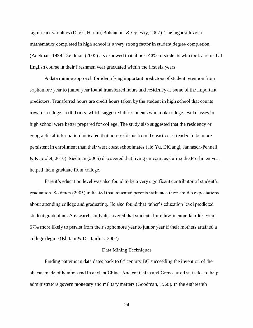
Data Mining Techniques
Finding patterns in data dates back to 6th
century BC succeeding the invention of the
abacus made of bamboo rod in ancient China. Ancient China and Greece used statistics to help
administrators govern monetary and military matters (Goodman, 1968). In the eighteenth
25
century, two branches of statistics evolved. The two branches were classical statistics and
Bayesian statistics. Classical statistics was inspired from mathematical works of Laplace and
Gauss, which considered the joint probability. Bayesian statistics, on the other hand, considered
the probability of an event occurring will be equal to the probability of its past occurrence
multiplied by the likelihood of its future occurrence (Nisbet, Elder, & Miner, 2009). Data mining
techniques use either approach.
Data mining is a comparatively new field in statistics. One of the early definitions of data
mining from Frawley et al. (1991) defined data mining as the non trivial extraction of implicit,
previously unknown, and potentially useful information from data. John (1997) explained data
mining as a new name for a previous process of finding patterns in data. John clarifies that the
search for patterns in data has been going on in different fields for a long time, but a common
name like data mining brought all these different fields together to focus on universal
resolutions.
Knowledge discovery and data mining are very closely related. “Knowledge discovery in
databases is the non-trivial process of identifying valid, novel, potential useful, and ultimately
understandable patterns in data” (Fayyad, Piatetsky-Shapiro, Smyth, & Uthurusamy, 1996). The
relationship between knowledge discovery in databases (KDD) and data mining is shown in
Figure 2.4.
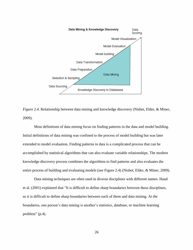
26
Figure 2.4. Relationship between data mining and knowledge discovery (Nisbet, Elder, & Miner,
2009).
Most definitions of data mining focus on finding patterns in the data and model building.
Initial definitions of data mining was confined to the process of model building but was later
extended to model evaluation. Finding patterns in data is a complicated process that can be
accomplished by statistical algorithms that can also evaluate variable relationships. The modern
knowledge discovery process combines the algorithms to find patterns and also evaluates the
entire process of building and evaluating models (see Figure 2.4) (Nisbet, Elder, & Miner, 2009).
Data mining techniques are often used in diverse disciplines with different names. Hand
et al. (2001) explained that “It is difficult to define sharp boundaries between these disciplines,
so it is difficult to define sharp boundaries between each of them and data mining. At the
boundaries, one person’s data mining is another’s statistics, database, or machine learning
problem” (p.4).

27
Data mining techniques allow researchers to build models from data repositories
(databases). These data mining techniques have the ability to analyze the entire database without
prior assumptions about any relevant linkages in the data. This kind of analysis does not involve
any statistician’s presumption about outcomes, which yields better results in finding patterns in
the data (Chopoorian, Witherell, Khalil, & Ahmed, 2001).
Hand et al. (2000) summarized some of the major data mining activities as follows:
1. Exploratory data analysis: includes techniques that help in inspecting a data set
using graphical charts and descriptive statistics;
2. Descriptive modeling: includes finding probability distributions, finding
relationships between models, and partitioning the data into groups;
3. Predictive modeling: includes building a statistical model to predict one variable
using another variable;
4. Discovering patterns and rules: includes activities from finding combinations of
items that occur frequently in transaction databases; and
5. Retrieval by content: includes activities of finding patterns in a new data set
similar to some know pattern of interest.
Data Mining Applications in Higher Education
Data mining techniques are extensively used in business applications. Nearly all data
mining techniques used in business applications can be applied in solving higher education
problems. Luan (2002) clarifies some data mining questions in the business sector and their
equivalent in higher education:
1. Business question: Who are my most profitable customers? (Equivalent in higher
education: Who are the students taking more credit hours?);

28
2. Business question: Who are my repeat website visitors? (Equivalent in higher
education: Which students are likely to return for more classes?);
3. Business question: who are my loyal customers? (Equivalent question in higher
education: Which students persist and graduate?);
4. Business question: who is likely to increase their purchase? (Equivalent in higher
education: Which alumni are likely to donate?); and
5. What clients are likely to defect to my rivals? (Equivalent in higher education:
what type of courses can we offer to keep our students?)
Data mining applications as they relate to enrollment, retention, and graduation are
discussed next.
Enrollment
Gonzalez and DesJardins (2002) tested how predictive modeling can be used to study
enrollment behavior. Authors used artificial neural networks to help predict which students are
more likely to apply to a large research based university in the mid-west. The neural network
model was compared with a logistic regression model, where the neural network model yielded a
misclassification rate of around 80% compared to a logistic regression model, which yielded a
misclassification rate of around 78%.
Chang (2006) used data mining predictive modeling to augment the prediction of
enrollment behaviors of admitted applicants at a large state university. Chang used classification
and regression trees (CART), logistic regression and artificial neural networks in predicting
admissions. CART yielded 74% classification rate, neural network with 75% classification rate,
and logistic regression with 64% classification rate.
29
In a similar study by Antons & Maltz (2006), they compared logistic regression, decision
trees, and neural networks in enrollment management through a partnership between the
admissions office, a business administration master's-degree program, and the institutional
research office at Willamette University, Oregon. Logistic regression classified 49% of the
enrollees and 78% of the non-enrollees.
In a research study at a California state university, researchers used support vector
machines and rule based predictive models to predict total enrollment headcount of students. The
total headcount consisted of Freshmen, transfer, continuing and returned students. This data
mining approach built predictive models for new, continued and returned students, respectively
first, and then aggregated their predictive results from which the model for the total headcount
was generated (Aksenova & Meiliu Lu, 2006).
Nandeshwar and Chaudhari (2009) used ensemble models to find causes of student
enrollment using admissions data. They used West Virginia University’s data warehouse to build
data mining models to predict student enrollment. They evaluated the model using cross-
validation, win-loss tables and quartile charts. The authors also used subset selection and
discretization techniques to reduce 287 variables to one and explained student enrollment
decision using rule based models. The model accuracy was around 83%.
Kovaic (2010) at Open Polytechnic of New Zealand examined variables in pre-
identifying successful and unsuccessful students. He found that classification and regression
trees (CART) were the best data mining models with an overall classification of 60.5%. They
also found that ethnicity, course program and course block to be some of the variables that
separated successful students from unsuccessful students.
30
Student Success and Graduation
One of the earliest studies of data mining application in student graduation used TETRAD
II2, a program developed in Carnegie Mellon University’s Department of Philosophy.
Researchers used this program with a database containing information of around 200 U.S.
Colleges, collected by the US News and World Report magazine. Average test score was found
to be one of the major factors affecting graduation. Researchers used ordinary least squares
multiple regression to find that test scores explained about 50% of variance in freshmen retention
rate and about 62% of the variance in graduation rate. They also applied regression to a group of
41 top ranking colleges and found about 68% of variance in Freshmen retention rate and 77% of
variance in graduation rate could be explained (Druzdzel & Glymour, 1994).
Hardgrave et al. (1994) compared neural networks and traditional techniques in
predicting graduate student success in a MBA program. Authors showed that traditional
techniques like regression analysis are not effective in predicting success or failure of graduate
students. They found that non- parametric procedures such as neural networks performed at least
or better than traditional methods.
Sanjeev and Zytkow (1995) used data mining applications in understanding university
enrollment to find ways to increase it. Authors used 49er, a software program developed by
Zytkow and Zembowicz (1993), which discovers knowledge in the form of regularities,
statements of the form “Pattern P holds for data in range R.” They found that “good high
school” students had the highest credit hours, financial aid had a huge impact on retention, and
remedial teaching did not help retain academically under prepared students.
Cripps (1996) used data mining techniques with admissions data for students who did not
meet entrance requirements. Cripps used feed forward neural network architecture with a back
31
propagation learning function and the logistic activation functions. This neural network model
was applied to around 17,500 student transcripts. The neural networks model showed that age,
gender, race, ACT scores, and reading level were significant predictors of graduation, earned
hours, and GPA.
Hunt (2000) compared neural networks with back-propagation and stepwise logistic
regression models in predicting student success. Hunt used data from two Freshmen cohorts with
enrollment variables available during admissions process and found that stepwise logistic
regression did a better job than neural networks in predicting persistence and graduation. Hunt
found that high school GPA, high school rank, financial need, and number of placement courses
were statistically significant predictors.
Massa and Puliafito (1999) used a new data mining application based on Markov chains
to find patterns in university leavers. Researchers used data from 1978-1998 and observed
samples of 15,000 students at the University of Genoa, Italy. They found patterns in data for the
high-risk population in order to design policies to reduce student leaving rates.
Stewart and Levin (2001) used predictive models to identify student characteristics
associated with persistence and success in the administration of justice (ADJ) program at Blue
Ridge Community College, Virginia. They used CLEMENTINE, a SPSS data mining package to
discover patters and relationships in students from the ADJ program and transfer students. The
authors found that GPA, cumulative hours attempted and cumulative hours completed without
the ADJ courses were significant variables. Additionally, the neural network model showed that
age, race, financial aid awards, and participation in developmental educational programs were
significant predictors of student characteristics.
32
Luan (2002) examined the theoretical basis for data mining techniques using a case study
to predict whether enrolled community college students would transfer to a four-year institution.
The data mining model created a profile of the transferred students predicting which student
currently enrolled in a community college will transfer so that the college can use intervention
programs for students who need assistance. Luan used two rule induction algorithms, neural
networks, C5.0, and a version of classification and regression trees known as C&RT in SPSS.
C&RT algorithm had the best classification rate compared to all other models.
Veitch (2004) investigated correlates of high school dropping out using chi-squared
automated interaction detector (CHAID), a decision tree data mining technique. Veitch used a k-
fold cross validation technique with k = 25, which showed that around 11% of students who did
not leave out were classified as non-leavers and GPA was the most significant variable.
Researchers at Industrial University of Santander, Colombia used a C-mean algorithm
and C4.5 algorithm to study academic achievement success and failure. They applied the C-mean
algorithm on statistically homogenous data subsets generating a group of qualitatively defined
clusters and then used the selected clusters were used in the C4.5 algorithm. Researchers found
that high scores on pre-university tests and students who were younger had a higher probability
of academic performance (Salazar, Gosalbez, Bosch, Miralles, & Vergara, 2004).
Barker et al. (2004) at University of Oklahoma used nonlinear discriminant methods like
neural networks and support vector machines for classifying student graduation behavior from
diverse student variables. Principal component method was used to reduce the number of
variables. The authors partitioned data into different ways for analysis, the first method involved
data for all three cohorts combined into a larger pool of students, the second method involved
using training data with all the students in a given year and testing the following year, and the
33
third method included training and testing within each cohort. Barker et al. (2004) found that the
overall misclassification rate was around 33% and reduced variable datasets had much higher
misclassification than complete datasets.
Superby et al. (2006) at Catholic University of Mons, Belgium used discriminant
analysis, random forests, decision trees, and neural networks to determine factors influencing
student achievement of first-year university students. Authors used a survey administered to 533
first-year university students and then constructed a database in which each student was
described based on attributes such as age, parent’s education level, and student’s university
perceptions. Data mining techniques were used to classify high risk, medium risk, and low risk
and found that scholastic history and socio-economic background were the most significant
predictors.
Herzog (2006) used student demographic, academic, residential, financial information,
American College Test’s (ACT), parent’s data and NSC data for identifying transfer students to
predict retention. The author used neural networks, logistic regression, and decision trees with
forty predictor variables to estimate retention and 79 variables to forecast time to degree (TTD).
Decision trees with C5.0 algorithm was the best model with 85% classification rate, 83% correct
classification rate for degree completion for three year or less, and 93% correct classification for
degree completion time in six years or more. Herzog concluded that decision trees and neural
networks performed as well as regression models.
Sujitparapitaya (2006) used National Student Clearinghouse data to describe how data
mining techniques were applied to examine critical predictors influencing decisions of first-time
freshmen on their one-year retention. There were three options for target variables 1) remaining
at their current institution; 2) transferring to another institution; and 3) dropping out from
34
college. Sujitparapitaya used three different data mining techniques like multinomial regression,
C5.0 rule induction, and neural networks and found first-year college GPA to be one of the
significant variables.
Researchers at University of Central Florida used student survey and demographic data to
predict student development and retention. They used 285 variables to build decision tree and
logistic regression models. Three different decision trees using entropy, chi-square, and gini
index split criterion and stepwise logistic regression models was built. The authors found that
decision trees with entropy split criterion was the best model with 90% classification on the
validation data and 88% on testing data (Atwell, Ding, Ehasz, Johnson, & Wang, 2006).
Davis et al. (2007) at The University of Alabama used logistic regression, decision trees
and neural network data mining techniques to find important variables predicting student
retention. The retention model predicted around 200 freshmen as being at risk to leave the
institution after their first year of college. The authors sent at risk student profile information to
their respective advisors for early intervention.
Campbell (2008) used four different data mining techniques: logistic regression,
automatic cluster detection, decision trees, and neural networks, at Northern Arizona University
to predict student retention. Campbell indicated that predicting a six year graduation rate would
require longitudinal data of at least nine years and to implement a three-year graduation model
requires about three years of training data, six years to collect data, and six years to validate the
model, thus adding up to fifteen years of data. Campbell found high school grade point average,
English placement exam, parent’s income, loan burden, and college grade point average as some
of the important predictors of six-year student graduation.
35
Pittman (2008) at Nova Southeastern University applied data mining techniques to
student demographic and behavioral data for both full and part-time students. Pittman used
neural networks, Bayesian classification, decision trees and logistic regression in predicting
student retention. Pittman found that neural networks, Bayesian classification, and decision tree
induction are comparable to logistic regression. Pittman segmented data into several
homogenous groups and concluded that the data mining approach could be used to isolate
student persistence differently for different groups of data.
Radney (2009) at California State University, Bakersfield, created a linear discriminant
function to predict an extensive range of persistence levels of first-time Freshmen students, by
identifying pre and early student variables. Radney used 17 predictor variables that included
personal, external, and institutional aspects. He found that high school GPA and first-year GPA
to be some of the most significant variables to student retention.
Lin et al. (2009) evaluated different student retention models and tested their impact on
prediction results. The authors developed 20 retention modeling systems based on a combination
of four retention modeling methodologies (neural networks, logistic regression, discriminant
analyses and structural equation modeling). The input variables ranged from 9 to 71 different
variables and contained cognitive and/or non-cognitive factors. The authors found that the neural
network method produced the best prediction results and models that combined both cognitive
and non-cognitive data performed better than just cognitive or non-cognitive models.
Hendricks (2000) at Baylor University used data mining techniques to investigate student
variables that were related to graduation status of students of some Texas public technical
colleges. Graduation status of a student was defined as three years after initial enrollment. Some
of the important variables related to graduation were Texas Academic Skills program (TASP)
36
test exemption status, TASP test passage status and economic-disadvantaged classification
of students. Other significant variables identified included designation in special populations,
limited English proficiency, displaced homemaker, and single parent.
Bailey (2006) used the Integrated Postsecondary Education Data System (IPEDS)
to develop a model to predict student graduation rates. IPEDS is a database system that holds
information from most higher education institutions. Bailey collected data for over 5,000
institutions and used classification and regression trees (CART) to find out some of the important
characteristics that impacted graduation rates.
Eykamp (2006) used multiple approaches including data mining techniques to examine
how time to graduation is associated with varying numbers of advanced placement units.
Yingkuachat et al. (2007) used the Bayesian belief network (Bayesnet) to analyze the predictor
variables that impacted vocational, undergraduate, and graduate student’s education
accomplishment. Results showed that GPA, parents career, family income, and high school GPA
were some of the important predictors.
The review of literature for data mining studies related to enrollment, retention, and
graduation indicated that the following data mining techniques proved to be the most useful:
logistics regression, decision trees, and neural networks. Research also indicated random forests,
a relatively newer data mining technique was one of the most accurate learning algorithms.
Therefore this study focused on comparing these four data mining techniques. A comparison
was made to determine which model was more effective in identifying characteristics of at risk
students and students themselves. Once at risk students are successfully identified it is paramount
that effective interventions programs be developed, administered, and examined for their utility.

37
Research Questions
1. What are some of the most important characteristics of first-time Freshmen students
who graduate from The University of Alabama?
2. Which of the data mining techniques: logistic regression, decision tree, random
forests, and artificial neural networks provide a better classification result in
predicting student graduation at The University of Alabama?
3. What characteristics identify first-time Freshmen students who might not graduate
from The University of Alabama?
38
CHAPTER III:
METHODS AND PROCEDURES
Data Source
The data analyzed in this research was obtained from the Office of Institutional Research
and Assessment (OIRA) at The University of Alabama. Data was analyzed for first-time
Freshmen students entering The University of Alabama from the fall semester of 1995 until the
fall semester of 2005. The dataset included only first-time entering undergraduates that begin the
first fall term of their academic career as full time (12 or more credits) students. Those who start
as ‘part-time’ students were not included in the dataset. Although OIRA’s databases have student
retention data until fall 2010, fall 2005 was chosen as the last year for analyses since students
graduated within six years from their enrollment. Also, there was not any graduation information
about students who started after fall 2005.
The data was downloaded from the OIRA datamart, which serves as the institution’s
official source of data for internal analyses as well as state and federal mandatory reporting on
student enrollment, student credit hour production, course-section instructional loads, student
persistence and graduation, and faculty and professional staff headcounts and salaries. The data
was extracted primarily from the University’s enterprise resource planning system (ERP), which
is a SunGard Banner ERP and provides transactional data for the day-to-day operations of the
institution. Official reporting data are extracted from the ERP at specified dates during the
academic year, known as official reporting dates (ORD). SAS programs were used to extract the
39
data from the ERP and load them into the OIRA datamart. Both data sources are Oracle
databases, so the data transfer was from Oracle to Oracle.
The data for this research was extracted from the OIRA datamart by a SAS program and
provided as a SAS dataset. The data included demographic and academic information entering
first-time Freshmen cohorts that entered the University from 1995 to 2005. In accordance with
the Family Educational Rights and Privacy Act (FERPA), the confidentially of all the students
with data in this dataset was protected by deleting from the dataset all personal identifying data
including student name, social security number, student campus identification number, and date
of birth. A dummy student record identifier was created so that students could be tracked over
time in the dataset without externally identifying the individual. A workspace directory was
created on the OIRA local network to house this dataset and all programs and data files
associated with this research. All additional data file cleaning and manipulation was done using
SAS®. Additionally ACT student data was also used to include more relevant variables. Data
integration was performed using SAS programs by merging ACT data with University of
Alabama student data with respect to unique student record identifiers.
Assumptions
It was assumed that the student data in the Office of Institutional Research and
Assessment database was accurate. The following assumption is rational for the reason that the
data was utilized frequently by OIRA in student data analyses for generating reports and results
at The University of Alabama. Also, any errors and corrections were assumed to be minor and
will not have any significant effect on the results of this research. Missing data was assumed to
be missing completely at random. Data missing completely at random is explained as the
probability that an observation is missing does not depend on the value it would have assumed
40
(Rubin, 1976), which means the probability of the missing values in one of the variables is
dissimilar to the value of the variable itself or to values of any other variables. The data was
assumed to be completely independent, which means that the effect of each variable on the target
variable (graduation) is not affected by the effect of any other variable.
Sampling Technique
The usual practice for cross-validating models is to split the data randomly into 70%-80%
to build the model and then use the rest 20%-30% for model evaluation. The random sample
used for training or evaluation might not be a good representation of the population. This
method of splitting the data had reliability problems and did not produce good results and
accuracy rate varied among similar datasets (Witten & Frank, 2005). Stratification method of
sampling ensures that each class is appropriately represented in training and evaluation datasets.
Also, the most excellent technique is to split the data multiple times and then evaluate the
original number. Data can be split ‘v’ different times so that each case is in the test data once,
this method is known as v-fold cross-validation (Nisbet, Elder, & Miner, 2009). When ‘v ‘is
equal to 10, the method is known as ten-fold cross validation.
Ten-fold cross-validation uses a stratified random sample technique to divide the entire
dataset into ten mutually exclusive sets. Stratification sampling divides the entire dataset into ten
different parts with equal proportions of students who graduated and students who did not
graduate in each set. Nine out of 10 sets are used as training data to build models and the data is
run through the remaining one dataset. A classification error rate is calculated for the model and
stored as an independent test error rate for the first model. Next, a second model is constructed
with a different set of nine samples and then a test error rate is calculated. The same process is
41
repeated ten times resulting in ten individual models. The classification error rates for all ten
models are then averaged. The optimum design parameters were chosen to minimize the error.
The cross-validation method gives better accuracy because the mean is more accurate
than a single experiment (Nisbet, Elder, & Miner, 2009). Logistic regression, Decision tree,
Random forests, and neural network models were built using the ten-fold cross-validation
method. The models were compared using receiver operating characteristic curves and
misclassification rates.
Missing Values
Logistic regression and neural networks necessitate complete observations; otherwise if
any portion of the observation is missing then both models completely ignore the entire row for
model building. Also, decision trees and random forests can model missing data as a genuine
value, distribute missing values to a node, and also distribute missing values over all the
branches. Although there are several statistical procedures for imputing/replacing missing values,
a list-wise deletion method was adopted in this research. A list-wise deletion method deletes the
entire record from the analysis if any variable in the model has a missing value. This technique is
secured when the data are missing completely at random and completely independent (Nisbet,
Elder, & Miner, 2009), which are the assumptions in this research. Moreover, the data set in data
mining analyses are usually enormous and therefore deleting a few observations will not impede
results of the model.
Variables
The dataset was compiled by tracking first-time Freshmen students entering in the fall
semester at The University of Alabama (UA) starting from 1995 through 2005. The variables
included in the study were associated with student characteristics. The dependent or target
42
variable was a binary variable, graduation. Graduation in this research is defined as a first-time
Freshmen student entering in the fall semester who graduates with an undergraduate degree from
The University of Alabama within the first six years of enrollment. The set of potential
predictors included the following:
1. Demographics: This set of predictors included gender, ethnicity, residency status
(in state or out of state), and distance from home. Residency status of students at
the University of Alabama is established based on the Alabama code 16-64. Also,
Alabama residents for tuition purposes are defined by the Alabama code and the
University Of Alabama Board Of Trustees rule. Distance from home was
calculated based on distance from University of Alabama to students’ hometown;
2. High School Information: The predictors included overall average High school
Grade Point Average (GPA), High school English GPA, High School Math GPA,
and Advanced Placement (AP) credit. Advanced Placement (AP) credits are
course credit hours earned by a high school student on standardized courses
offered in high school that are equivalent to undergraduate courses;
3. College characteristics: These variables included first semester GPA, and first
semester Earned Hours, and status. First semester GPA is the average GPA of a
student of all first semester courses. Total earned hours are the total number of
credit hours earned at the end of semester. Graduation was the target variable
showing if the student graduated from The University of Alabama or not. Status -
students with less than 12 earned credit hours were classified as part-time students
and students greater than 12 earned credit hours were classified as full-time
students; and
43
4. ACT information: ACT student profile included work ACT score, work
information, and college choice. The SAT and the ACT scores are standardized
tests for high school achievements and college admissions. The University of
Alabama accepts both SAT and ACT scores; therefore, all applicants at the
University of Alabama must take either SAT or ACT exams in order to apply for
admission. Some students take either SAT or ACT and sometimes both;
therefore, there might be missing values for some students in both SAT or ACT
scores. The concordance table published by the ACT uses a formula to convert
SAT combined scores to ACT composite scores (see Appendix A). For students
with SAT scores, their SAT scores were converted to composite ACT scores. For
students who took both SAT and ACT only their ACT score was considered.
5. Work information variable indicated if the student wanted to work while in
college and college choice indicated if the student chose The University of
Alabama as first choice of college. Table 3.1 gives a complete description of all
the variables.
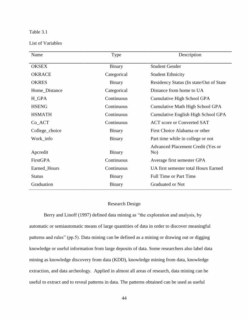
44
Table 3.1
List of Variables
Name Type Description
OKSEX Binary Student Gender
OKRACE Categorical Student Ethnicity
OKRES Binary Residency Status (In state/Out of State
Home_Distance Categorical Distance from home to UA
H_GPA Continuous Cumulative High School GPA
HSENG Continuous Cumulative Math High School GPA
HSMATH Continuous Cumulative English High School GPA
Co_ACT Continuous ACT score or Converted SAT
College_choice Binary First Choice Alabama or other
Work_info Binary Part time while in college or not
Apcredit Binary
Advanced Placement Credit (Yes or
No)
FirstGPA Continuous Average first semester GPA
Earned_Hours Continuous UA first semester total Hours Earned
Status Binary Full Time or Part Time
Graduation Binary Graduated or Not
Research Design
Berry and Linoff (1997) defined data mining as “the exploration and analysis, by
automatic or semiautomatic means of large quantities of data in order to discover meaningful
patterns and rules” (pp.5). Data mining can be defined as a mining or drawing out or digging
knowledge or useful information from large deposits of data. Some researchers also label data
mining as knowledge discovery from data (KDD), knowledge mining from data, knowledge
extraction, and data archeology. Applied in almost all areas of research, data mining can be
useful to extract and to reveal patterns in data. The patterns obtained can be used as useful
45
information to increase income, cuts expenses, and any other kinds of benefits for any
organization. Data mining is usually done using business intelligence software that uses a
number of analytical tools for analyzing data. With the help of this software data miners analyze
data from many different aspects, sort out data, and summarize the relationships identified.
Finding correlations or patterns among dozens of fields in large databases, data mining is an
interdisciplinary exercise in which statistical analytical tools play a vital role. Disciplines like
database technology, artificial intelligence, and pattern recognition routinely use data mining
techniques.
Some of the major data mining activities include Exploratory Data Analysis (EDA). John
Tukey’s (1977) article was one of the most influential works in EDA. The data exploration
actions include visual techniques that help analysts view a dataset in terms of summary. This
helps in getting a feel of trends and pattern analysis (Tukey, 1977). Exploratory Data Analysis is
a philosophy detailing with how to dissect a dataset, discover, inquire, and finally make
interpretations. Some of the basic statistical exploratory methods include examining distribution
of variables to check for patterns, reviewing large correlation matrices for coefficients that meet
certain thresholds, or examining multi-way frequency tables. EDA can also include multivariate
exploratory techniques, which are designed specifically to identify patterns in multivariate data
sets. Some of the techniques include factor analysis, cluster analysis, canonical correlation,
decision trees, and neural networks.
While approaching a statistical problem an analyst may have some prior hypotheses that
need to be tested. For example, if educational researchers in a university are interested in
whether a recent increase in the fee structure has led to a decrease in student enrollment, the
analysts would test the hypothesis that the enrollment has decreased and would use hypothesis
46
testing procedures. Some methods in classical hypothesis testing includes: Z-test, t-test, or F-test,
so there are a number of hypothesis tests throughout the statistical literature, including time
series analysis and non-parametric tests.
When using data mining procedures, analysts do not always have prior notions of the
expected relationships among the variables or have any notions about any expected outcomes
from the dataset; therefore data mining techniques do not necessarily have a priori hypotheses.
Since data mining datasets are usually very large, analysts often prefer to use exploratory data
analysis. This method allows the analysts to
1. Delve into the dataset;
2. Examine the interrelationships among the attributes;
3. Identify interesting subsets of the observations; and
4. Develop an initial idea of possible associations between the attributes and the
target variable.
Data mining techniques can find patterns that are present but are hidden in large
institutional datasets. This methodology merges statistical techniques, machine learning
algorithms, and visual illustration techniques to discover patterns in institutional data. In order to
assess the significant variables contributing to student graduation, this research used four
different data mining predictive models: logistic regression, decision trees, random forests, and
neural networks. These four predictive models can identify the most significant variables
impacting student graduation and also predict the percentage of students who do not graduate.
This study also tested the accuracy of the four data mining models, which can provide additional
information and insights about what kind of data mining models work best in higher education
data mining analyses.
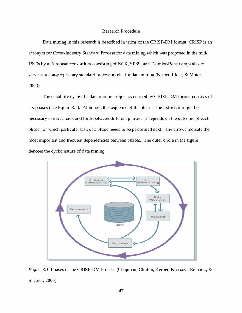
47
Research Procedure
Data mining in this research is described in terms of the CRISP-DM format. CRISP is an
acronym for Cross-Industry Standard Process for data mining which was proposed in the mid-
1990s by a European consortium consisting of NCR, SPSS, and Daimler-Benz companies to
serve as a non-proprietary standard process model for data mining (Nisbet, Elder, & Miner,
2009).
The usual life cycle of a data mining project as defined by CRISP-DM format consists of
six phases (see Figure 3.1). Although, the sequence of the phases is not strict, it might be
necessary to move back and forth between different phases. It depends on the outcome of each
phase , or which particular task of a phase needs to be performed next. The arrows indicate the
most important and frequent dependencies between phases. The outer circle in the figure
denotes the cyclic nature of data mining.
Figure 3.1. Phases of the CRISP-DM Process (Chapman, Clinton, Kerber, Khabaza, Reinartz, &
Shearer, 2000)
48
Figure 3.1 shows the CRISP-DM process for data mining. The process is described as
cyclic:
1. Business Understanding: The first stage in data mining emphasizes the
understanding of project objectives and then translates those objectives to a data
mining problem definition. This stage may include defining clear business
objectives, evaluating the business environment, and preparing clear goals and
objectives. Some of the activities in the initial stage might include identifying the
target variable, listing all the important predictor variables, acquiring the suitable
institutional dataset for analyses and modeling, generating descriptive statistics
for some variables, etc.
2. Data Understanding: This stage starts with data collection and getting used to the
data to identify potential patterns in the data. The second stage involves activities
like data acquirement, data integration, initial data description, and data quality
assessment activities. Data has to be acquired before it can be used. Although
this stage appears to be obvious, it is very important to identify various data
resources available. It is usual for multi-national companies to have their data
stored in data repositories; for other situations like a university setting it might be
different. Therefore it is very important for the data miner to use or acquire
accurate data to address the business problem. It is also important to integrate
different datasets together so that it can be exploited. Data might exist in different
formats like in spreadsheets, csv, word, etc.; therefore, it is imperative to build a
road map to integrate everything to a common format. All the necessary data at
this stage is merged to form a single dataset containing all variables. After

49
merging, data might be in different formats or variables represented in different
forms and will have to be formatted accordingly. To maintain consistency, data
mining tools like SAS enterprise miner can import any kind of format and convert
it to a SAS data file. Finally, in this stage it is important to describe the data to
understand and make sure the data is a good fit for answering all the objectives.
3. Data Preparation: As the name implies, the third stage involves preparing the data
for analyses. This stage might involve transforming variables and creating proper
formats to fit the data mining software. Some of the important activities in the
data preparation stage is data cleaning, transformation (if necessary), and handling
missing values. An overall summary of activities in the initial exploration are:
(Han & Kamber, 2006)
Data Cleansing
Data Transformation
Data Imputation
Data Filtering
Data Abstraction
Data Reduction
Data Sampling
Dimensionality Reduction
Data Derivation
4. Modeling: The fourth stage in data mining involves building and selecting
models. The usual practice is to create a series of models using different statistical
algorithms or data mining techniques, also known as ensemble models. Another

50
technique is to create samples of data and compare or combine results. Bootstrap,
jackknife resampling, and V-fold cross validation are some techniques which use
sample data. (Nisbet, Elder, & Miner, Handbook of Statistical Analysis & Data
Mining Applications, 2009). In most of the data mining software, after specifying
important model assumptions, it is important to set parameters because sometimes
the options in the algorithm are default. Many modeling algorithms like neural
networks, decision trees, and logistic regressions start with various default
settings. Data mining software like Enterprise miner has an options tab to set
parameter values.
5. Evaluation: This stage involves evaluating the models built in the model building
stage. The most common way to evaluate models is to verify their performances
on the test datasets. Some very effective techniques for doing this, using various
tables and graphs, are coincidence tables, lift charts, ROI curves, normal
probability charts etc. Also an easy evaluation of all the models is to observe the
number of correct predictions compared to the total number of predictions. If that
percentage is relatively high, we might conclude that the model was a success.
6. Deployment: The final stage involves using the model selected in the previous
stage and applying it to new/future data in order to generate predictions or
estimates of the expected outcome. As shown in Figure 3.1, feedback of model
deployment results to the database and feedback of model deployment results to
the business understanding phase.
51
Software
This research used data mining software to investigate the most important variables that
are associated with graduation and also to answer specific research questions. SAS enterprise
Miner from SAS Inc. and R programming language were used as the data mining software for all
the analyses. SAS Enterprise Miner facilitated data mining analyses to generate very high
accurate predictive models based on all the data available from across the University of Alabama
campus. For all other data cleaning, data merging, and exploration SAS 9.2® was used. In
mining the data, the target variable was graduation and all other variables will be used as
predictors.
Model Comparison Techniques
Model comparison techniques illustrate the accuracy of a model. Model evaluation is an
iterative process in which all competing models are evaluated based on accuracy. If accuracy of
the model is too low, the model is underfit and when the accuracy is too high the model is overfit
(Nisbet, Elder, & Miner, 2009). An overfit model results in excellent model accuracy with
respect to the training data. Therefore it is very important to cross-validate models to select the
best generalized model.
Receiver Operating Characteristic (ROC)
The receiver operating characteristic (ROC) chart illustrates a graphical display that
evaluates the forecasting precision of a predictive model. ROC curve describes the discriminate
capacity of the predictive model and is applied to binary targets (Provost & Fawcett, 1997). The
ROC curves display the sensitivity and the specificity of the model for a cutoff value or a
threshold value. For example, let graduation labels y ∈ {0/No, 1/Yes} have a threshold or cutoff
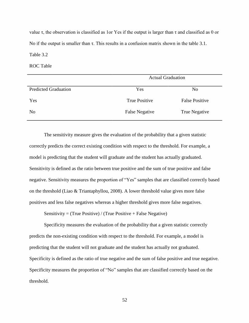
52
value τ, the observation is classified as 1or Yes if the output is larger than τ and classified as 0 or
No if the output is smaller than τ. This results in a confusion matrix shown in the table 3.1.
Table 3.2
ROC Table
Actual Graduation
Predicted Graduation Yes No
Yes True Positive False Positive
No False Negative True Negative
The sensitivity measure gives the evaluation of the probability that a given statistic
correctly predicts the correct existing condition with respect to the threshold. For example, a
model is predicting that the student will graduate and the student has actually graduated.
Sensitivity is defined as the ratio between true positive and the sum of true positive and false
negative. Sensitivity measures the proportion of “Yes” samples that are classified correctly based
on the threshold (Liao & Triantaphyllou, 2008). A lower threshold value gives more false
positives and less false negatives whereas a higher threshold gives more false negatives.
Sensitivity = (True Positive) / (True Positive + False Negative)
Specificity measures the evaluation of the probability that a given statistic correctly
predicts the non-existing condition with respect to the threshold. For example, a model is
predicting that the student will not graduate and the student has actually not graduated.
Specificity is defined as the ratio of true negative and the sum of false positive and true negative.
Specificity measures the proportion of “No” samples that are classified correctly based on the
threshold.
53
Specificity = (True Negative) / (False Positive + True Negative)
The 1 – Specificity value measures the evaluation of the probability that a given statistic
incorrectly predicts the condition does not exist with respect to the threshold. For example, a
model is predicting that the student will graduate while the student has actually not graduated.
The ROC curve is a typical practice for summarizing classifier accuracy over a range of
tradeoffs between the true positive and false positive mistake rates (Swets, 1988). The ROC
curve is plotted with sensitivity in the Y-axis and 1 – Specificity values in the X axis. The area
under the ROC curve gives the biased presentation for a binary classification problem. The ROC
curve shows the estimation of the probability that the output of a randomly selected validation
sample from the “NO” population will be less than or equal to that of a randomly selected
training sample from “Yes” population. The choice of cut-off describes the trade-off between
sensitivity and specificity. In an ideal situation the cut-off should represent high values of both so
that the model can predict students who graduated and students who did not graduate. A low cut
off increases true positive and false negative and decreases false positive and true negative and
therefore gives a higher sensitivity. On the other hand, a higher cut off gives a lower sensitivity.
Figure 3.2 shows a ROC curve with sensitivity/percent true value plotted on the vertical
axis and 1 – Specificity or percent false positive plotted on the horizontal axis. Each point on the
curve corresponds to a particular cut-off or threshold. The perfect point on the curve will be [0,
1] which shows that all students who graduated are classified correctly and students who did not
graduate are misclassified as students who graduated. The area under the curve (AUC) is an
established metric for determining ROC. The AUC comparisons between different models can
establish a supreme relationship between classifiers. The best model is the curve that is almost in
parallel to the vertical axis or coinciding with the vertical axis. Higher AUC value represents

54
better classification or discrimination between students who graduated and students who did not
graduate with respect to training data.
Figure 3.2. Example ROC Curve.
Misclassification Rate
For binary classification scenarios, the misclassification rate gives the overall model
performance with respect to the exact number of categorizations in the training data. The
objective of the predictive model is to maximize the number of accurate classifications. A
confusion matrix similar to a ROC curve can also be created representing the binary
classifications for the training data. Table 3.3 shows predicted graduation as the row variable and
actual graduation as the column variable.
0.00
0.10
0.20
0.30
0.40
0.50
0.60
0.70
0.80
0.90
1.00
0.00 0.20 0.40 0.60 0.80 1.00
Sen
siti
vit
y
1 - Specificity
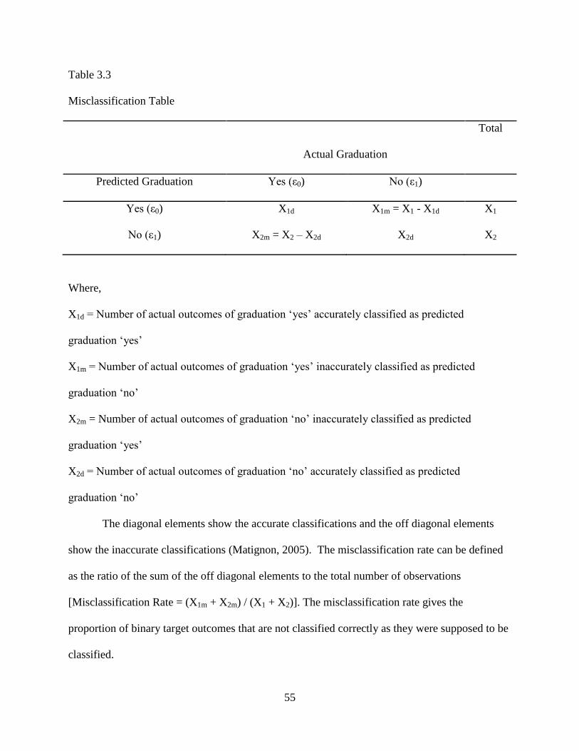
55
Table 3.3
Misclassification Table
Actual Graduation
Total
Predicted Graduation Yes (ε0) No (ε1)
Yes (ε0) X1d X1m = X1 - X1d X1
No (ε1) X2m = X2 – X2d X2d X2
Where,
X1d = Number of actual outcomes of graduation ‘yes’ accurately classified as predicted
graduation ‘yes’
X1m = Number of actual outcomes of graduation ‘yes’ inaccurately classified as predicted
graduation ‘no’
X2m = Number of actual outcomes of graduation ‘no’ inaccurately classified as predicted
graduation ‘yes’
X2d = Number of actual outcomes of graduation ‘no’ accurately classified as predicted
graduation ‘no’
The diagonal elements show the accurate classifications and the off diagonal elements
show the inaccurate classifications (Matignon, 2005). The misclassification rate can be defined
as the ratio of the sum of the off diagonal elements to the total number of observations
[Misclassification Rate = (X1m + X2m) / (X1 + X2)]. The misclassification rate gives the
proportion of binary target outcomes that are not classified correctly as they were supposed to be
classified.
56
Similarly, accuracy rate can be defined as the ratio of the sum of the diagonal elements to the
total number of observations [Accuracy Rate = (X1d + X2d) / (X1 + X2)]. A superior model will
have a high accuracy and low misclassification rate.
Data Mining Models
This study compared the statistical predictive data mining models: logistic regression,
decision tree, random forests, and neural networks based on the review of literature in Chapter II.
Each of these models were optimized to fit the student graduation data and then evaluated to
determine the best data mining model. Logistic regression, decision trees, and neural network
predictive models used in this research were the most popular models used in the statistical data
mining process and random forests is a relatively recent data mining model, which has not been
applied in higher education data mining applications. These data mining models are designed to
extract useful information and make inferences from large datasets. Data mining is inspired by
the computing and storing power of computers; therefore, analyzing data and creating many
models and evaluating the best model are familiar methods in a data mining research design.
Logistic Regression
In the early 1980s, statisticians were dealing with more intricate real world problems.
Statistical approaches became too restraining for investigating nonlinear relationships in large
data sets. Mathematical researchers continued investigating along the lines of classical statistics
and developed nonlinear versions of parametric statistics. Some of these nonlinear methods for
discrete distributions were the Logit model, the Probit model and the Generalized Linear model
(Nisbet, Elder, & Miner, 2009). Logistic regression uses the Logit model. This is one of the
techniques used in analyzing a categorical dependent variable. It provides an association between
the independent variables and the logarithm of the odds of a categorical response variable.
57
However when a categorical variable has only two responses, then it is called a binary logistic
regression model. Since the target variable graduation is a binary (yes/no) response a binary
logistic regression model was used. Logistic regression analysis applies maximum likelihood
estimation after transforming the dependent variable (graduation) into a Logit variable (the
natural log of the odds of the dependent response occurring or not); therefore, logistic regression
will estimate the odds that an existing student graduated or not graduated.
Ordinary least-squares multiple regression model is represented as follows:
Y = + + + …….. + + ε (1)
Where , , , …….., represent the model parameters. These are constants, whose true
value remains unknown, which are estimated from the data using the least-squares estimates, ε,
which represents the error term (Belsey, Kuh, & Welsch, 2004).
Some of the assumptions associated with a multiple regression error term are:
1. Constant Variance: The variance of the error term is constant regardless of the
value for , ,…..
2. Independence: The error values are independent
3. Normally Distributed: The error term is a normally distributed random variable.
In other words the error term is an independent normal variable with µ=0 and
variance, .
Logistic regression has gained reputation in data mining techniques because it does not
require any of the above mentioned assumptions (Fadlalla, 2005).
The binary outcome for the target variable graduation (graduated (1)/not graduated (0))
can be represented as the conditional mean of Y given X = x, represented as E(Y|x). Where
E(Y|x) is the expected value of the target variable graduation for a given value of predictor.
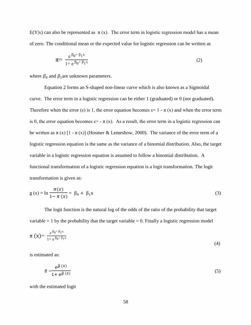
58
E(Y|x) can also be represented as π (x). The error term in logistic regression model has a mean
of zero. The conditional mean or the expected value for logistic regression can be written as
π= e 0+ 1x
1+ e 0+ 1x (2)
where and are unknown parameters.
Equation 2 forms an S-shaped non-linear curve which is also known as a Sigmoidal
curve. The error term in a logistic regression can be either 1 (graduated) or 0 (not graduated).
Therefore when the error (ε) is 1, the error equation becomes ε= 1 - π (x) and when the error term
is 0, the error equation becomes ε= - π (x). As a result, the error term in a logistic regression can
be written as π (x) [1 - π (x)] (Hosmer & Lemeshow, 2000). The variance of the error term of a
logistic regression equation is the same as the variance of a binomial distribution. Also, the target
variable in a logistic regression equation is assumed to follow a binomial distribution. A
functional transformation of a logistic regression equation is a logit transformation. The logit
transformation is given as:
g (x) = ln
= (3)
The logit function is the natural log of the odds of the ratio of the probability that target
variable = 1 by the probability that the target variable = 0. Finally a logistic regression model
π = e 0+ 1x
1+ e 0+ 1x
(4)
is estimated as:
=
(5)
with the estimated logit
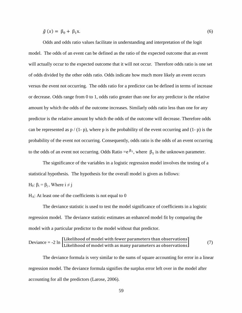
59
. (6)
Odds and odds ratio values facilitate in understanding and interpretation of the logit
model. The odds of an event can be defined as the ratio of the expected outcome that an event
will actually occur to the expected outcome that it will not occur. Therefore odds ratio is one set
of odds divided by the other odds ratio. Odds indicate how much more likely an event occurs
versus the event not occurring. The odds ratio for a predictor can be defined in terms of increase
or decrease. Odds range from 0 to 1, odds ratio greater than one for any predictor is the relative
amount by which the odds of the outcome increases. Similarly odds ratio less than one for any
predictor is the relative amount by which the odds of the outcome will decrease. Therefore odds
can be represented as p / (1- p), where p is the probability of the event occurring and (1- p) is the
probability of the event not occurring. Consequently, odds ratio is the odds of an event occurring
to the odds of an event not occurring. Odds Ratio = , where is the unknown parameter.
The significance of the variables in a logistic regression model involves the testing of a
statistical hypothesis. The hypothesis for the overall model is given as follows:
H0: i = j , Where i ≠ j
HA: At least one of the coefficients is not equal to 0
The deviance statistic is used to test the model significance of coefficients in a logistic
regression model. The deviance statistic estimates an enhanced model fit by comparing the
model with a particular predictor to the model without that predictor.
Deviance = -2 ln
(7)
The deviance formula is very similar to the sums of square accounting for error in a linear
regression model. The deviance formula signifies the surplus error left over in the model after
accounting for all the predictors (Larose, 2006).
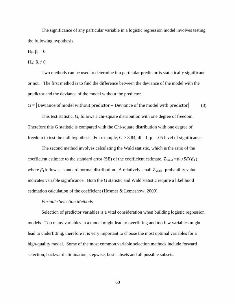
60
The significance of any particular variable in a logistic regression model involves testing
the following hypothesis.
H0: i = 0
HA: i ≠ 0
Two methods can be used to determine if a particular predictor is statistically significant
or not. The first method is to find the difference between the deviance of the model with the
predictor and the deviance of the model without the predictor.
G = – (8)
This test statistic, G, follows a chi-square distribution with one degree of freedom.
Therefore this G statistic is compared with the Chi-square distribution with one degree of
freedom to test the null hypothesis. For example, G > 3.84, df =1, p = .05 level of significance.
The second method involves calculating the Wald statistic, which is the ratio of the
coefficient estimate to the standard error (SE) of the coefficient estimate. ZWald = ,
where follows a standard normal distribution. A relatively small ZWald probability value
indicates variable significance. Both the G statistic and Wald statistic require a likelihood
estimation calculation of the coefficient (Hosmer & Lemeshow, 2000).
Variable Selection Methods
Selection of predictor variables is a vital consideration when building logistic regression
models. Too many variables in a model might lead to overfitting and too few variables might
lead to underfitting, therefore it is very important to choose the most optimal variables for a
high-quality model. Some of the most common variable selection methods include forward
selection, backward elimination, stepwise, best subsets and all possible subsets.
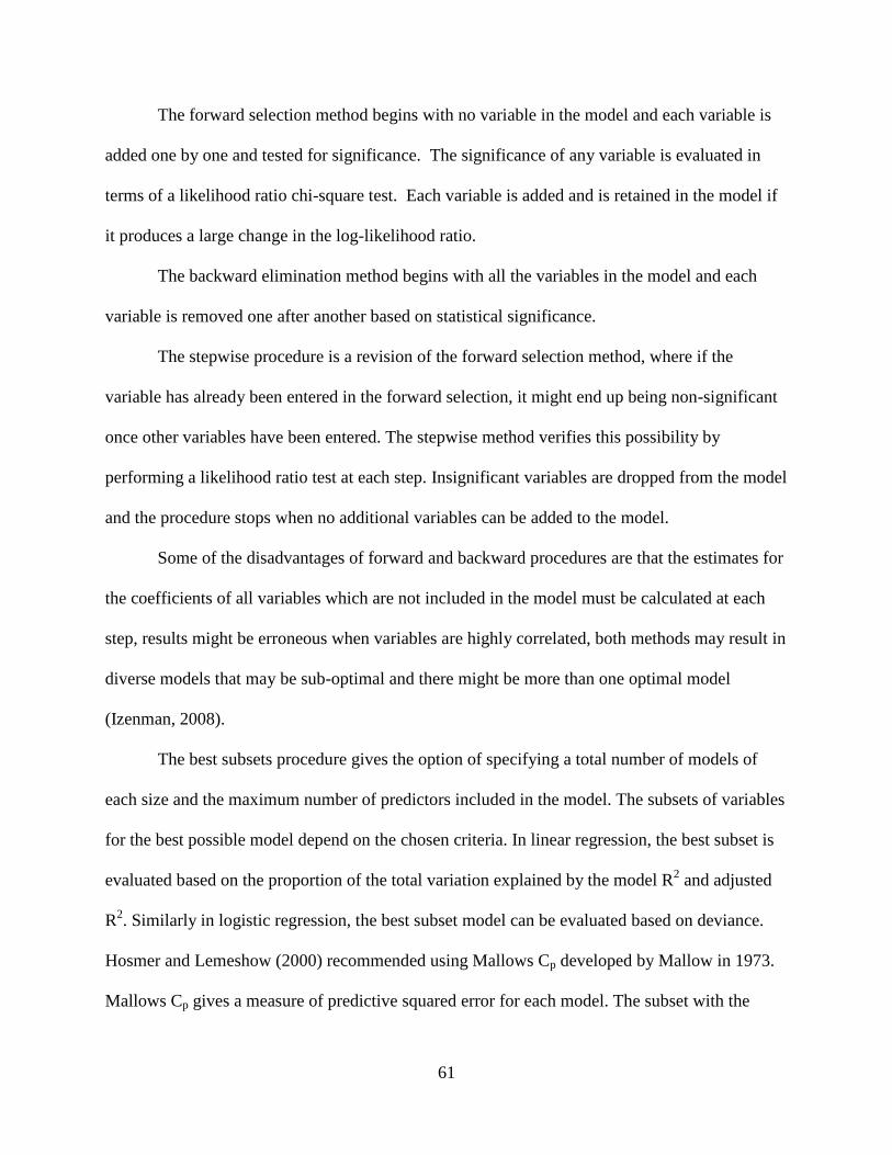
61
The forward selection method begins with no variable in the model and each variable is
added one by one and tested for significance. The significance of any variable is evaluated in
terms of a likelihood ratio chi-square test. Each variable is added and is retained in the model if
it produces a large change in the log-likelihood ratio.
The backward elimination method begins with all the variables in the model and each
variable is removed one after another based on statistical significance.
The stepwise procedure is a revision of the forward selection method, where if the
variable has already been entered in the forward selection, it might end up being non-significant
once other variables have been entered. The stepwise method verifies this possibility by
performing a likelihood ratio test at each step. Insignificant variables are dropped from the model
and the procedure stops when no additional variables can be added to the model.
Some of the disadvantages of forward and backward procedures are that the estimates for
the coefficients of all variables which are not included in the model must be calculated at each
step, results might be erroneous when variables are highly correlated, both methods may result in
diverse models that may be sub-optimal and there might be more than one optimal model
(Izenman, 2008).
The best subsets procedure gives the option of specifying a total number of models of
each size and the maximum number of predictors included in the model. The subsets of variables
for the best possible model depend on the chosen criteria. In linear regression, the best subset is
evaluated based on the proportion of the total variation explained by the model R2 and adjusted
R2. Similarly in logistic regression, the best subset model can be evaluated based on deviance.
Hosmer and Lemeshow (2000) recommended using Mallows Cp developed by Mallow in 1973.
Mallows Cp gives a measure of predictive squared error for each model. The subset with the
62
smallest Cp value is selected as the best subset. Mallows Cp for any subset of p from q variables
is given as
Cp =
+ 2(p+1) – n. (9)
Where, is the Pearson’s Chi-square, is the Wald statistic (Hosmer & Lemeshow, 2000).
The concluding type of variable selection method in logistic regression is all possible
subsets procedure. All other modeling procedures use different approaches to find the optimal
model, however there is no assurance in finding the most optimal model using different
statistical criteria. The only way to guarantee optimal subsets is to execute all possible subsets.
Therefore, for an n variable model, there are 2n – 1 all possible logistic regression models to find
the optimal model (Larose, 2006). This approach to variable selection provides all possible
combinations of predictor variables with selection of the best model based on R2, Cp, or deviance
fit statistic.
Multicollinearity
Some selected variables in a regression model could result in multicollinearity. The
generated model will be checked for multicollinearity. Collinearity is a condition where two or
more predictors are highly correlated. This leads to instability in coefficient estimates, with
possible incoherent results. For example, a data set with severe collinearity may have a
significant deviance statistic, while having no significant Wald statistic for predictors. Highly
correlated variables tend to confound predictors in the regression model. Also examining
correlations among predictors may not reveal the problem, whereas the Variance Inflation
Factors (VIFs) identify the presence of multicollinearity. SAS Enterprise Miner generates VIFs
for each predictor. Some research suggests eliminating one of the two variables with very high
63
VIF’s. Also, standardization prevents variability of one variable affecting a second variable
(Larose, 2006).
Four different logistic regression models were built using forward selection, backward
elimination, stepwise, and all possible subsets with graduation as the target variable.
Decision Trees
In 1984, UC Berkley and Stanford researchers Leo Breiman, Jerome Friedman, Richard
Olshen, and Charles Stone introduced Classification and Regression Tree (CART or C&RT)
methodology. Decision trees are ordered as a sequence of simple questions. The answers to
these simple questions conclude what might be the next question. This results in a network of
links that forms a tree-like structure. The network attempts to find strong associations between a
group of predictor variables and the target value. A set of input variables are recognized and are
grouped resulting in dividing the entire dataset based on different rules. The first rule splits the
data from the root node. Each rule allocates a data point to a link based on the value of the input
variable for that particular data point. The end of the tree is terminal leaf nodes. The terminal leaf
nodes have no preceding questions. Algorithms in decision trees recognize different ways of
splitting a dataset into branches that look similar to branches in a tree. Decision trees can be
used in predictive modeling for classification purposes.
The tree like structure helps with human short-term memory where more complicated
relationships can be effectively understood. Decision trees can be used to classify an occurrence
like graduation (yes/no) based on different variables. Decision trees are a functional exploratory
technique, which still uses classical statistical methods. Decision trees are extensively used for
their ease of use, interpretability, flexibility with different levels of measurement, and its
prediction strength with diversity of data (Ville, 2006).
64
A simple decision tree is shown in Figure 3.3. The root node is the top most node
representing the first split variable which can either be continuous or discrete. For each node in a
decision tree, some type of partition rule is usually chosen. This results in choosing the best
partition of its levels. The best partitions are usually determined by using a goodness measure
that measures the performance gain from subdividing the node. The partition rules are applied
one after another which results in the tree like structure as shown in Figure 3.3. Partition rule for
the root node in this simple case result in a two way split. The two way split at the root node
results in two different nodes, which are connected through a link. Same splitting rules apply for
these two nodes. There could be more than a two-way split as well. The bottom most nodes of
the decision trees are called terminal nodes or leaves and these leaves do not have any further
splits. For each leaf in the tree the decision links presents an exclusive path for decision rules.
Once the tree is fully built and decision rules have been established, these rules can be used to
predict a new node value based on new data. In predictive modeling for student graduation, the
decision rules will help in predicting the value for the variable graduation (yes/no).
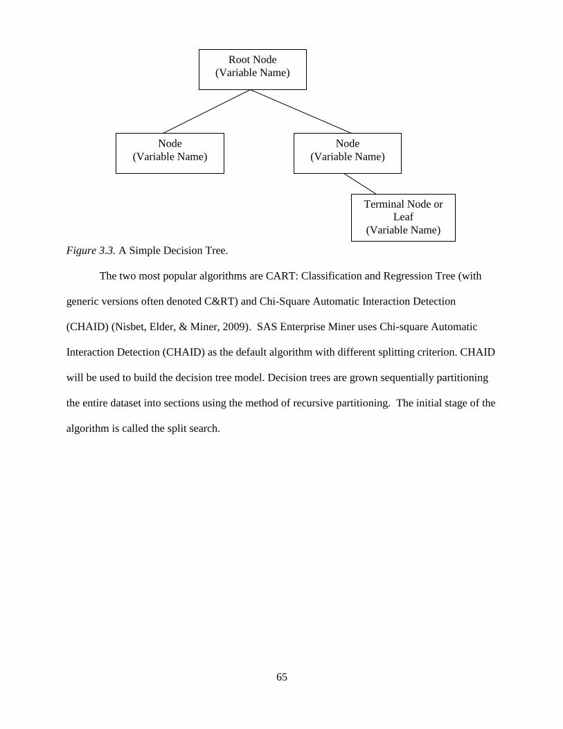
65
Figure 3.3. A Simple Decision Tree.
The two most popular algorithms are CART: Classification and Regression Tree (with
generic versions often denoted C&RT) and Chi-Square Automatic Interaction Detection
(CHAID) (Nisbet, Elder, & Miner, 2009). SAS Enterprise Miner uses Chi-square Automatic
Interaction Detection (CHAID) as the default algorithm with different splitting criterion. CHAID
will be used to build the decision tree model. Decision trees are grown sequentially partitioning
the entire dataset into sections using the method of recursive partitioning. The initial stage of the
algorithm is called the split search.
Root Node
(Variable Name)
Node
(Variable Name)
Node
(Variable Name)
Terminal Node or
Leaf
(Variable Name)
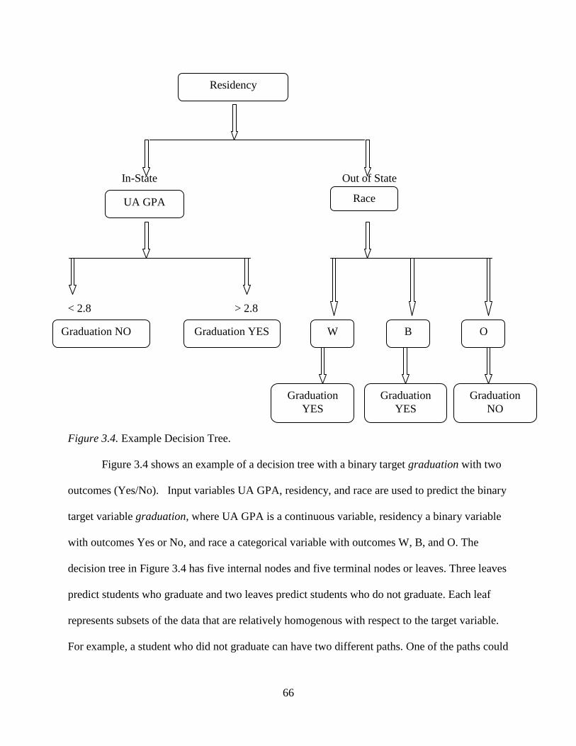
66
In-State Out of State
< 2.8 > 2.8
Figure 3.4. Example Decision Tree.
Figure 3.4 shows an example of a decision tree with a binary target graduation with two
outcomes (Yes/No). Input variables UA GPA, residency, and race are used to predict the binary
target variable graduation, where UA GPA is a continuous variable, residency a binary variable
with outcomes Yes or No, and race a categorical variable with outcomes W, B, and O. The
decision tree in Figure 3.4 has five internal nodes and five terminal nodes or leaves. Three leaves
predict students who graduate and two leaves predict students who do not graduate. Each leaf
represents subsets of the data that are relatively homogenous with respect to the target variable.
For example, a student who did not graduate can have two different paths. One of the paths could
Residency
UA GPA
Graduation NO Graduation YES
Race
W B O
Graduation
YES
Graduation
YES
Graduation
NO
67
be an in-state resident with a UA GPA less than 2.8 who did not graduate. The other path could
be an out of state resident with other race who did not graduate..
This split search algorithm begins by selecting an input for portioning the training data.
For binary input, only two values serve as a potential split point. The groups combined with the
predicted or the target variable creates a 2X2 contingency table or a confusion matrix. The null
hypothesis is given as
H0: V1 = V2: variable 1 and variable 2 are independent
H0: V1 ≠ V2: variable 1 and variable 2 are not independent
The independence of counts in the table is evaluated using a Pearson’s chi-square
statistic. High Pearson chi-square values indicate the independence of counts in the table
columns. A very high difference in outcome proportions specifies a good split. The Pearson chi-
square is calculated using the following formula
χ2
= (observed Frequency – Expected Frequency)
2 / Expected Frequency) (10)
The same Pearson chi-square is applied to all input variables and a probability value also
known as a p-value is calculated for each split. A low p-value is similar to a high Pearson chi-
square. The p-value is calculated as follows:
P-Value = P (χ2 > Calculated χ
2 | Null hypothesis is true) (11)
For huge datasets this p-value can be very close to zero. Therefore, this p-value is
reported using logworth, where the logworth = - Log (Chi-square p-value). The algorithm
evaluates every input variable and target variable and the best split is chosen in accordance with
the logworth value (Sarma, 2007). Also, when calculating the chi-square value for testing
independence of columns, it is possible to attain very high chi-square values or low p-values
when in reality the columns are not independent or there is no difference in proportions between
68
split branches. Since there are so many splits occurring in building a decision tree, the likelihood
of having a larger logworth or smaller p-value increases. In order to overcome this problem, the
p-value of every test is magnified by a factor equal to the number of tests being performed. This
magnified p-value is known as a Bonferroni correction. SAS Enterprise Miner automatically
applies these Bonferroni corrections to the logworth calculations for each input. These
corrections known as Kass adjustments decrease the logworth of a split by a quantity equal to the
log of the number of separate input values (Kass, 1980).
Figure 3.4 show that residency was chosen as the first split at the root node with the
highest logworth. Consequently, observations with value in state branch to the left and
observations with value out of state branch to the right. For a split to occur, SAS Enterprise
Miner uses a default chi-square p-value of 0.20 corresponding to a logworth of 0.7.
Significance of a second split and all the succeeding splits depend on the previous splits;
so this split search algorithm features a multiple comparison problem. Therefore the p-values
have to be adjusted for these previous splits. This adjustment for the number of previous splits
depends on the number of splits, known as depth adjustment. This depth is measured as the
number of branches from the path of root node to the present node where splitting has to take
place. The p-value is multiplied with a depth multiplier to compensate for previous splits. The
general depth multiplier for binary splits is 2d. For a depth of three splits from the number of
branches from the root node, the depth multiplier would be 23 = 8. This value will be multiplied
with the p-value. The same depth multiplier can be used to increase the threshold value of the
logworth by log10 (2) * d. The threshold value becomes more stringent as it goes further down
the tree; therefore the depth adjustment limits the size of the tree. The size of the tree can be
controlled using either a threshold value or the adjusted p-value. One other way to control the

69
tree size is to set the leaf size or the split size to a specified number. A node will be not be split if
it has less than the specified number of leaf size or split size. The data is partitioned according to
the best split and this in turn creates a new second partition rule. The process goes on until there
are no more splits. The resulting tree is known as a maximal tree (Sarma, 2007).
Pruning
A decision tree with all the split rules will end up as the largest possible tree. The
maximal tree does a great job predicting the target variable with the training data but usually not
as good with the validation data; therefore, the maximal tree has a generalization problem.
Model generalization and model complexity can be addressed using a method called pruning.
The tree has to be pruned to the right size in order to find the optimal tree. One split is removed
from the maximal tree at each step, which results in two trees at the first pruning step.
Subsequently one more split is removed from the previous tree, which results in another tree. If
the maximal tree is T, then the first pruning step results in T-1 tree, T-2, T-3, T-4, and so on.
Now all these different decision tree models are evaluated to find the optimal tree. Binary
decision predictions can be evaluated using criteria based on misclassification. When primary
decisions are matched with the primary outcomes then it is called a true positive and when
secondary decisions are matched with secondary outcomes then it is called a true negative.
Therefore, predictions can be rated by their accuracy based on the proportion between the
prediction and actual outcome. A model with a lower proportion misclassified is chosen as the
best decision tree model.
Random Forests
Brieman (2001) developed random forests algorithm that uses the concept of bagging and
builds a large collection of decision trees. Breiman (1996) created Bagging also known as
70
bootstrap aggregating, one of the earliest and simplest ensemble modeling techniques. The
bagging algorithm is similar to bootstrapping where data is resampled to create separate
prediction estimates and then aggregated together. In bagging, a fixed number of independent
samples is created by replacement. The bagged estimates of the predicted values are calculated
by refitting the statistical model to calculate the fitted values for each bootstrap sample of equal
size, then dividing by the number of bootstrap samples.
bag (x) =
(12)
where bag (x) is the bagging estimate from B bootstrap samples. Random forest is an
extensive modification of bagging that builds a series of de-correlated decision trees and then
averages them. An ensemble decision tree model is built based on multi classifier’s decision. A
final decision tree model is not made by one tree; instead several trees are constructed
independently and each tree is weighted for a comprehensive classification. As the number of
trees in the random forests increases the generalization error decreases with better predicting
power. Each bagged training set contains the same number of samples as the original training
data, but samples are randomly selected with replacement and are representative of two-thirds of
the data. The other one-third of data is used for classification performance. Each tree is grown
without pruning until the data at leaf nodes are homogenous or some other predefined stopping
criteria. Predictions are performed by running the one-third test sample through each tree and
each tree is assigned a vote based on the leaf node that receives the sample. A random forests
model does not require additional cross-validation unlike other models to get an unbiased
estimate of the test error. Following are the steps involved in building decision trees using
random forests:

71
1. A random sample of the number of observations is taken. Successive samples for
other trees are done with replacement without leaving out any observations;
2. Only ‘m’ variables are chosen from a set of variables, where m is much less than
actual number of variables. Increasing the number of variables increases the
correlation between trees and increases the predictive power of the tree;
3. Best split for each tree is done similarly as discussed in the decision tree section.
4. About one-third of the cases are used to create out of sample or testing data. This
testing data is used to calculate the error rate;
5. Average error rates will be calculated from all trees;
6. Significant variables are chosen by running test data set down the tree and then
the number of votes for the predicted class is counted;
7. Values in each variable are randomly changed and run down independently. Next
the measure of effect is calculated from the difference between number of votes
for unchanged tree and number of votes for changed tree; and
8. Average effect is calculated across all trees to find the most significant variables.
Brieman (2001) summarizes some of the important features of random forests as follows:
1. Better accuracy compared to other data mining predictive models;
2. Works competently with large datasets;
3. Can handle any number of input variables;
4. Produces unbiased estimates of the generalization error; and
5. Handles missing data by estimation and also maintains a better accuracy when
large proportion of the data is missing.

72
Neural Networks
Neural networks were based on the structure and function of the human brain. The human
brain has about 109 interconnected neurons and there can be numerous connections per neuron
approximately summing up to 60 trillion synapses (Garson, 1998). The actual functioning of
these neurons remains unknown. In 1943, McCulloch and Pitts proposed a mathematical version
of artificial neural networks models composed of binary valued neurons. This mathematical
version of neural networks was imitating the way nerve cells process information for enhancing
or plummeting transmitted signal (Silipo, 1999). Artificial neural network models are learning
algorithms that analyze any given classification problem. Interconnected “neurons” help in all
mathematical operations in transforming inputs to outputs (Abu-Mostafa, 1996). The concept of
neural networks got more popular and was extended for use with computers in the 1980s when
John Hopfied invented the back-propagation method. A typical neural network model consists of
inputs connected to hidden layers with the number of nodes and the hidden layers connected to
an output node.
Figure 3.5 shows a simple neural network model with one input, one target and one
single output variable. In terms of conventional regression analysis, the input in neural network
is analogous to an independent variable, output is analogous to a predicted value and target is
analogous to a dependent variable.
Figure 3.5. Simple Neural Network.
Input
Output Target

73
Figure 3.6 shows artificial neural networks with input layer, hidden layer, and an output
layer. The units are combined and connected into layers. Layers in a network are connected to
each other by connecting every unit in the first layer to every unit in the second layer. The input
layer is connected to the hidden layer by all the input variables, which represent the neurons in
the human brain. The input node with a linear summation function and a logistic or sigmoid
activation function connected to the output node is similar to a logistic regression predicting a
binary outcome. All the input units from the input layer are standardized using the equivalent
standardization method to have the identical unit of measurement. The hidden layers have the
same combination function and activation function. Because the output is a binary variable
(graduation), the activation process is represented by a logistic function. Also, all the units in
the output layer have the same combination function and error function.
Input Hidden Output
.
.
.
.
Figure 3.6. Neural Networks Architecture.
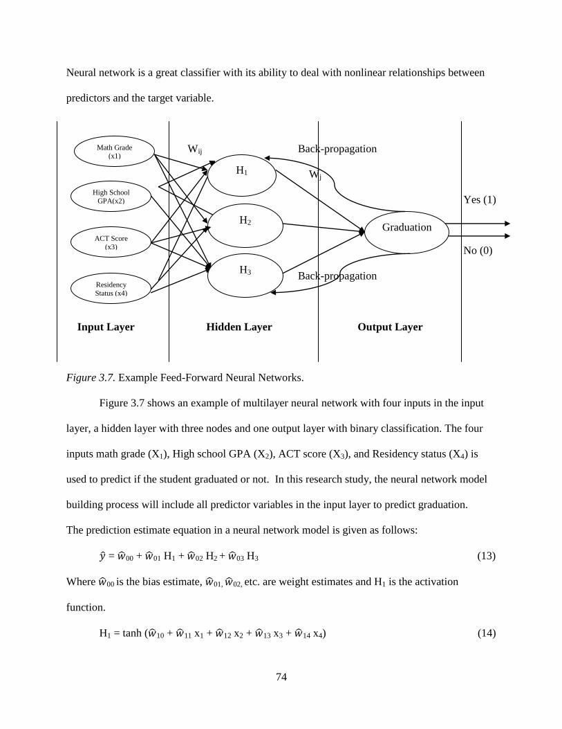
74
Neural network is a great classifier with its ability to deal with nonlinear relationships between
predictors and the target variable.
Wij Back-propagation
Wj
Yes (1)
No (0)
Back-propagation
Input Layer Hidden Layer Output Layer
Figure 3.7. Example Feed-Forward Neural Networks.
Figure 3.7 shows an example of multilayer neural network with four inputs in the input
layer, a hidden layer with three nodes and one output layer with binary classification. The four
inputs math grade (X1), High school GPA (X2), ACT score (X3), and Residency status (X4) is
used to predict if the student graduated or not. In this research study, the neural network model
building process will include all predictor variables in the input layer to predict graduation.
The prediction estimate equation in a neural network model is given as follows:
= 00 + 01 H1 + 02 H2 + 03 H3 (13)
Where 00 is the bias estimate, 01, 02, etc. are weight estimates and H1 is the activation
function.
H1 = tanh ( 10 + 11 x1 + 12 x2 + 13 x3 + 14 x4) (14)
Graduation
Math Grade (x1)
High School
GPA(x2)
ACT Score
(x3)
Residency
Status (x4)
H1
H3
H2
75
H2 = tanh ( 20 + 21 x1 + 22 x2 + 23 x3 + 24 x4) (15)
H3 = tanh ( 30 + 31 x1 + 32 x2 + 33 x3 + 34 x4) (16)
Figure 3.7 shows the weights represented as Wij to be assigned to each input node and
connected to the hidden layer. The other weights, Wj, are assigned to each node in the hidden
layer, which is connected to the output layer. These weights help in modeling non-linear
relationships between the input and output layers. As the number of nodes in the hidden layer
increases, the complexity of the neural network model increases and the model does a better job
in modeling non-linear relationships. One of the most complex problems in neural networks lies
in the selection of the number of nodes in the hidden layer. Selecting the right number of nodes
in the hidden layer is an important aspect of generalization of the neural network model. The
optimal number of nodes in the hidden layer depends on the number of observations, number of
input variables and the distribution of the training data. Too many nodes in the hidden layer can
cause overfitting of the model, implying that the model would do a great job with the trained
dataset, but not with a different dataset. On the other hand too few nodes in the hidden layer can
cause underfitting, implying that the model is a poor fit to the training data. The neural network
model is fit numerous times with a diverse number of hidden units and evaluated using
goodness-of-fit statistics. The network weights are adjusted iteratively to improve the predictive
power of the model with the process known as back-propagation. The steps involved in back-
propagation when predicting a binary response are as follows:
1. Weights (Wij and Wj) are assigned randomly to each connection and the sum of
input times their weight is calculated at each node;
2. A threshold value is specified below where the output is predicted at 0 and above
where it is predicted at 1;
76
3. Error is calculated as the expected prediction minus actual prediction and weights
are adjusted as error multiplied by output weight; and
4. Finally, the new weight for the second stage is calculated as the sum of the old
input weight and adjusted weights (Nisbet, Elder, & Miner, 2009). The same steps
are completed for all inputs and the iteration is continued through the data.
Therefore a neural network for a binary prediction is given as
Log
= 00 + 01 H1 + 02 H2 + 03 H3 (17)
(H1) = ( 10 + 11 x1 + 12 x2 + 13 x3 + 14 x4) (18)
(H2) = ( 20 + 21 x1 + 22 x2 + 23 x3 + 24 x4) (19)
(H3) = ( 30 + 31 x1 + 32 x2 + 33 x3 + 34 x4) (20)
The iterative learning technique of neural networks permits them to be very flexible and
adjustable to dynamic situations. For the same reason, neural networks are extensively used in
business environments especially in finance for forecasting business applications. Neural
Networks have been shown to be more accurate than traditional statistics. They can analyze
large sets of data with non-linear or linear target variables. They also do not require any
underlying assumptions associated with the distribution of data (Nisbet, Elder, & Miner, 2009).
One of the key disadvantages of neural network models includes the lack of explanatory
power; the hidden layer is not interpretable because of the unavailability of calculated weights.
Therefore it is sometimes termed as a “black box” (Nisbet, Elder, & Miner, 2009).
However, neural networks are good for prediction and estimation in cases where the
characteristics of data are available explicitly and understood (Berry & Linoff, 2004). Therefore

77
in this research study, since all the students’ characteristics are known, a neural network would
be an appropriate modeling technique.
Research Questions
1. What are some of the most important characteristics of first-time Freshmen students
who graduate from The University of Alabama?
2. Which of the data mining techniques: logistic regression, decision tree, random
forests, and artificial neural networks provide a better classification result in
predicting student graduation at The University of Alabama?
3. What characteristics identify first-time Freshmen students who might not graduate
from The University of Alabama?
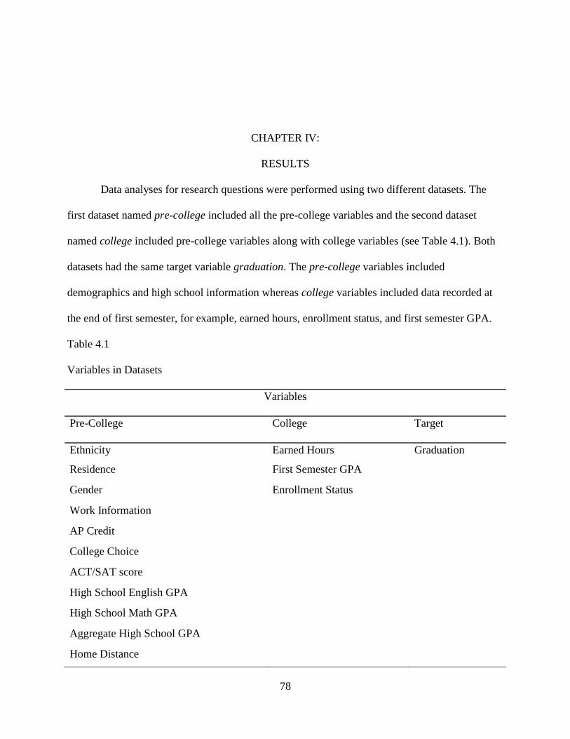
78
CHAPTER IV:
RESULTS
Data analyses for research questions were performed using two different datasets. The
first dataset named pre-college included all the pre-college variables and the second dataset
named college included pre-college variables along with college variables (see Table 4.1). Both
datasets had the same target variable graduation. The pre-college variables included
demographics and high school information whereas college variables included data recorded at
the end of first semester, for example, earned hours, enrollment status, and first semester GPA.
Table 4.1
Variables in Datasets
Variables
Pre-College College Target
Ethnicity Earned Hours Graduation
Residence First Semester GPA
Gender Enrollment Status
Work Information
AP Credit
College Choice
ACT/SAT score
High School English GPA
High School Math GPA
Aggregate High School GPA
Home Distance
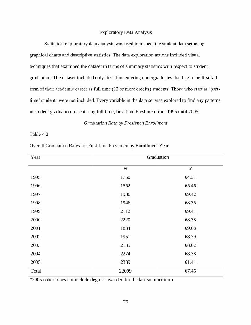
79
Exploratory Data Analysis
Statistical exploratory data analysis was used to inspect the student data set using
graphical charts and descriptive statistics. The data exploration actions included visual
techniques that examined the dataset in terms of summary statistics with respect to student
graduation. The dataset included only first-time entering undergraduates that begin the first fall
term of their academic career as full time (12 or more credits) students. Those who start as ‘part-
time’ students were not included. Every variable in the data set was explored to find any patterns
in student graduation for entering full time, first-time Freshmen from 1995 until 2005.
Graduation Rate by Freshmen Enrollment
Table 4.2
Overall Graduation Rates for First-time Freshmen by Enrollment Year
Year Graduation
N %
1995 1750 64.34
1996 1552 65.46
1997 1936 69.42
1998 1946 68.35
1999 2112 69.41
2000 2220 68.38
2001 1834 69.68
2002 1951 68.79
2003 2135 68.62
2004 2274 68.38
2005 2389 61.41
Total 22099 67.46
*2005 cohort does not include degrees awarded for the last summer term
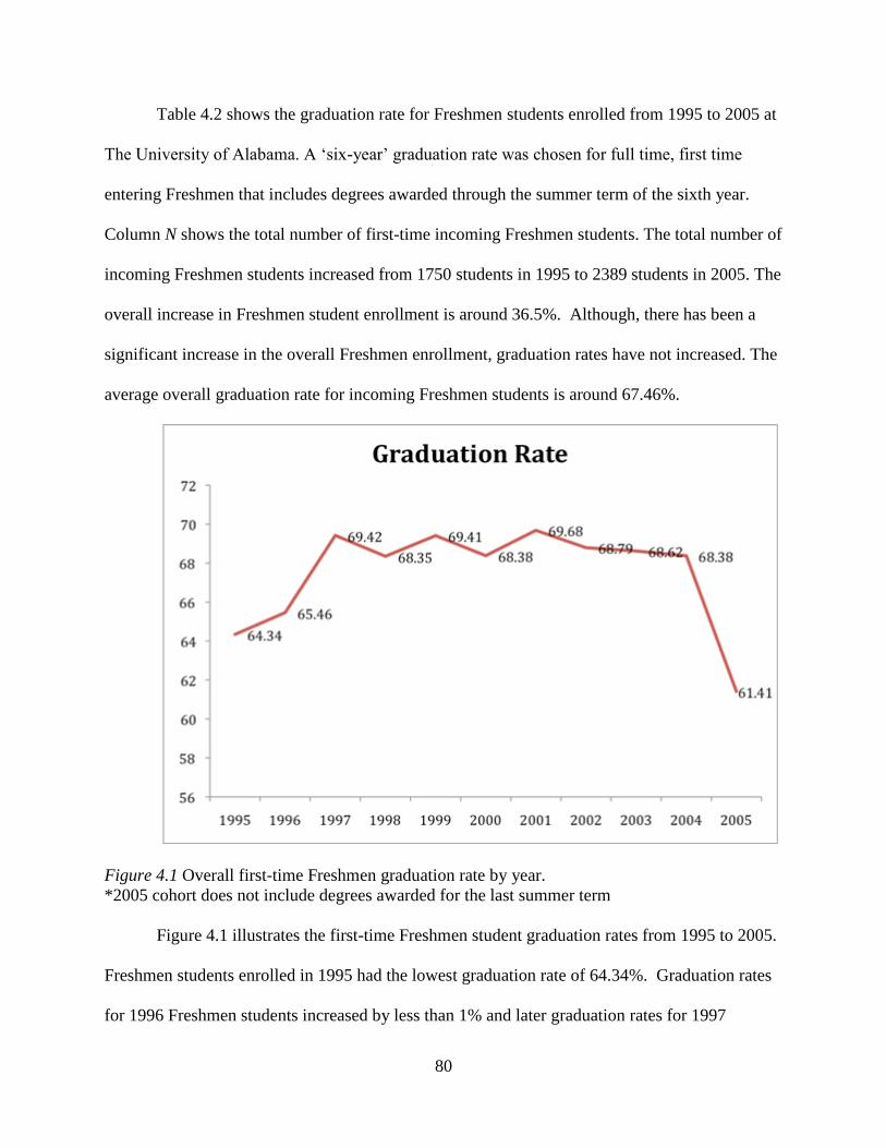
80
Table 4.2 shows the graduation rate for Freshmen students enrolled from 1995 to 2005 at
The University of Alabama. A ‘six-year’ graduation rate was chosen for full time, first time
entering Freshmen that includes degrees awarded through the summer term of the sixth year.
Column N shows the total number of first-time incoming Freshmen students. The total number of
incoming Freshmen students increased from 1750 students in 1995 to 2389 students in 2005. The
overall increase in Freshmen student enrollment is around 36.5%. Although, there has been a
significant increase in the overall Freshmen enrollment, graduation rates have not increased. The
average overall graduation rate for incoming Freshmen students is around 67.46%.
Figure 4.1 Overall first-time Freshmen graduation rate by year.
*2005 cohort does not include degrees awarded for the last summer term
Figure 4.1 illustrates the first-time Freshmen student graduation rates from 1995 to 2005.
Freshmen students enrolled in 1995 had the lowest graduation rate of 64.34%. Graduation rates
for 1996 Freshmen students increased by less than 1% and later graduation rates for 1997

81
Freshmen students increased by about 4%. Graduation rates for first-time Freshmen from 2002 to
2004 remained consistent at approximately 68%. In fact, graduation rates for students enrolled
from 1997 to 2004 did not fluctuate significantly. 2005 cohort does not include the degrees
awarded for the last summer term. Therefore the six-year graduation rates are lower for this
particular group. The estimated final graduation rate for first time Freshmen entering in 2005
will be around 68%.
Graduation Rate by Gender
Table 4.3
Graduation Rate for First-time Freshmen by Gender
Gender
Year Male Female
N % N %
1995 754 58.49 996 68.78
1996 608 63.82 944 66.53
1997 846 66.19 1090 71.93
1998 831 62.82 1115 72.47
1999 896 64.73 1216 72.86
2000 923 62.19 1297 72.78
2001 759 64.03 1075 73.67
2002 822 65.57 1129 71.12
2003 911 66.19 1224 70.42
2004 966 64.08 1308 71.56
2005 998 58.42 1391 63.55
Total 9314 63.29 12785 70.49
*2005 cohort does not include degrees awarded for the last summer term
82
Numbers in Table 4.3 shows the overall graduation rate in terms of gender for Freshmen
students enrolled from 1995 to 2005 at The University of Alabama. Column N shows the total
number of male and female first-time Freshmen students, respectively.
The total female enrollment constitutes around 58% compared to 42% for males. First-
time entering Freshmen female students in 2001 had the highest graduation rate of around
73.67% and Freshmen female students enrolled in 1996 had the lowest graduation rate of
66.53%.
The highest graduation rate for male students was 66.19% in both 1997 and 2003. The
lowest female graduation rate was close to the highest male graduation rate. Lastly, the overall
graduation rate for first-time freshmen females was 70.49% compared to 63.29% for males.
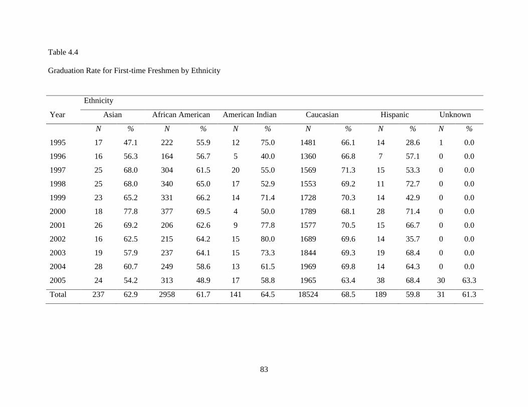
83
Table 4.4
Graduation Rate for First-time Freshmen by Ethnicity
Ethnicity
Year Asian African American American Indian Caucasian Hispanic Unknown
N % N % N % N % N % N %
1995 17 47.1 222 55.9 12 75.0 1481 66.1 14 28.6 1 0.0
1996 16 56.3 164 56.7 5 40.0 1360 66.8 7 57.1 0 0.0
1997 25 68.0 304 61.5 20 55.0 1569 71.3 15 53.3 0 0.0
1998 25 68.0 340 65.0 17 52.9 1553 69.2 11 72.7 0 0.0
1999 23 65.2 331 66.2 14 71.4 1728 70.3 14 42.9 0 0.0
2000 18 77.8 377 69.5 4 50.0 1789 68.1 28 71.4 0 0.0
2001 26 69.2 206 62.6 9 77.8 1577 70.5 15 66.7 0 0.0
2002 16 62.5 215 64.2 15 80.0 1689 69.6 14 35.7 0 0.0
2003 19 57.9 237 64.1 15 73.3 1844 69.3 19 68.4 0 0.0
2004 28 60.7 249 58.6 13 61.5 1969 69.8 14 64.3 0 0.0
2005 24 54.2 313 48.9 17 58.8 1965 63.4 38 68.4 30 63.3
Total 237 62.9 2958 61.7 141 64.5 18524 68.5 189 59.8 31 61.3
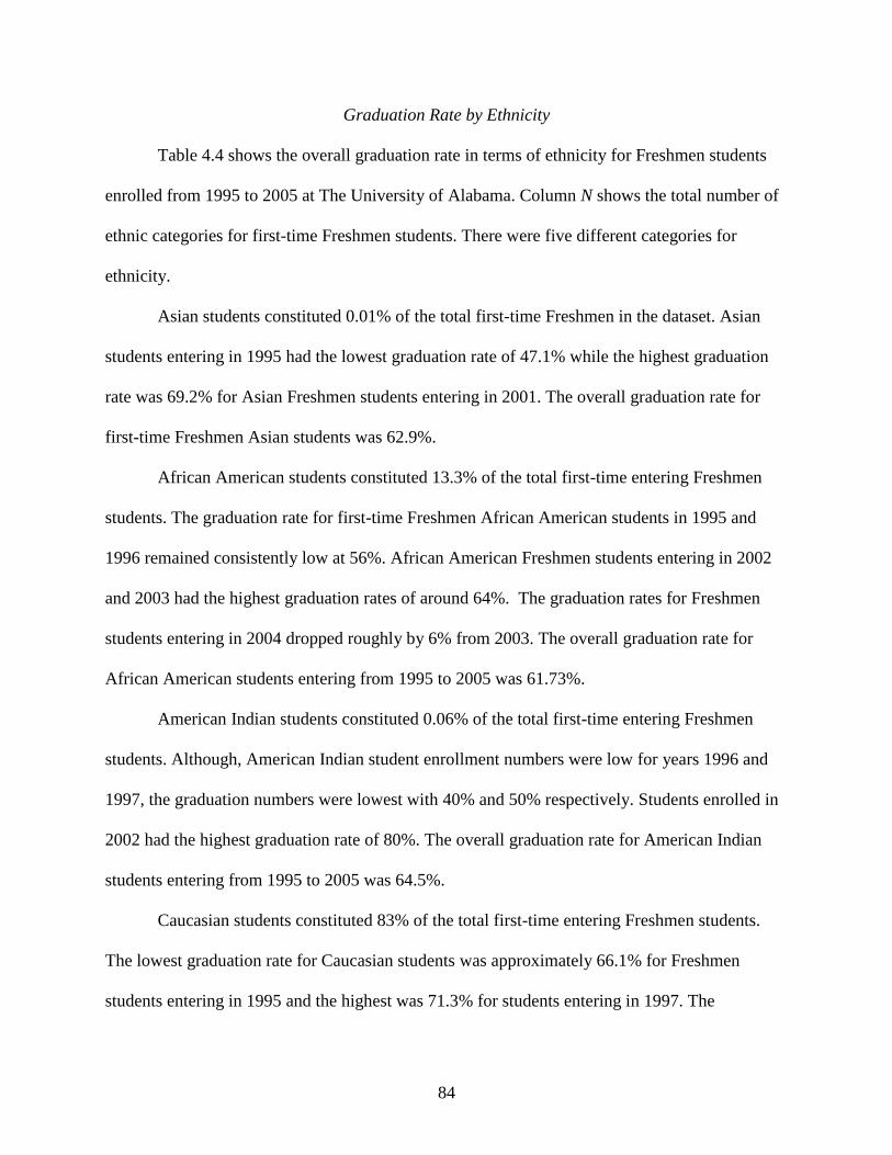
84
Graduation Rate by Ethnicity
Table 4.4 shows the overall graduation rate in terms of ethnicity for Freshmen students
enrolled from 1995 to 2005 at The University of Alabama. Column N shows the total number of
ethnic categories for first-time Freshmen students. There were five different categories for
ethnicity.
Asian students constituted 0.01% of the total first-time Freshmen in the dataset. Asian
students entering in 1995 had the lowest graduation rate of 47.1% while the highest graduation
rate was 69.2% for Asian Freshmen students entering in 2001. The overall graduation rate for
first-time Freshmen Asian students was 62.9%.
African American students constituted 13.3% of the total first-time entering Freshmen
students. The graduation rate for first-time Freshmen African American students in 1995 and
1996 remained consistently low at 56%. African American Freshmen students entering in 2002
and 2003 had the highest graduation rates of around 64%. The graduation rates for Freshmen
students entering in 2004 dropped roughly by 6% from 2003. The overall graduation rate for
African American students entering from 1995 to 2005 was 61.73%.
American Indian students constituted 0.06% of the total first-time entering Freshmen
students. Although, American Indian student enrollment numbers were low for years 1996 and
1997, the graduation numbers were lowest with 40% and 50% respectively. Students enrolled in
2002 had the highest graduation rate of 80%. The overall graduation rate for American Indian
students entering from 1995 to 2005 was 64.5%.
Caucasian students constituted 83% of the total first-time entering Freshmen students.
The lowest graduation rate for Caucasian students was approximately 66.1% for Freshmen
students entering in 1995 and the highest was 71.3% for students entering in 1997. The

85
graduation rates for Freshmen students entering from 2002-2004 remained consistent around
69%. The overall graduation rate for Caucasian students was 68.5%.
Hispanic students constituted 0.08% of the total first-time entering Freshmen students.
Students entering in 1995 had the lowest graduation rate of 28.6%. Also, graduation rates
decreased by more than 30% for students who entered in 2001 compared to students who entered
in 2002.
The two major ethnic categories in terms of enrollment were African American and
Caucasian students with 13.3% and 83%, respectively. On the whole, Caucasian students had a
higher graduation rate (68.5%) compared to African American students (61.7%). This is a 6.8%
difference between African American and Caucasian graduation rates.
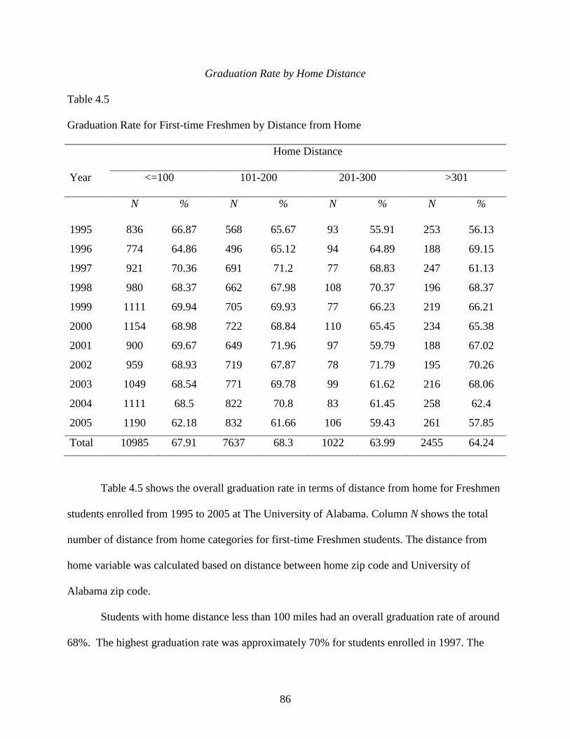
86
Graduation Rate by Home Distance
Table 4.5
Graduation Rate for First-time Freshmen by Distance from Home
Home Distance
Year <=100 101-200 201-300 >301
N % N % N % N %
1995 836 66.87 568 65.67 93 55.91 253 56.13
1996 774 64.86 496 65.12 94 64.89 188 69.15
1997 921 70.36 691 71.2 77 68.83 247 61.13
1998 980 68.37 662 67.98 108 70.37 196 68.37
1999 1111 69.94 705 69.93 77 66.23 219 66.21
2000 1154 68.98 722 68.84 110 65.45 234 65.38
2001 900 69.67 649 71.96 97 59.79 188 67.02
2002 959 68.93 719 67.87 78 71.79 195 70.26
2003 1049 68.54 771 69.78 99 61.62 216 68.06
2004 1111 68.5 822 70.8 83 61.45 258 62.4
2005 1190 62.18 832 61.66 106 59.43 261 57.85
Total 10985 67.91 7637 68.3 1022 63.99 2455 64.24
Table 4.5 shows the overall graduation rate in terms of distance from home for Freshmen
students enrolled from 1995 to 2005 at The University of Alabama. Column N shows the total
number of distance from home categories for first-time Freshmen students. The distance from
home variable was calculated based on distance between home zip code and University of
Alabama zip code.
Students with home distance less than 100 miles had an overall graduation rate of around
68%. The highest graduation rate was approximately 70% for students enrolled in 1997. The
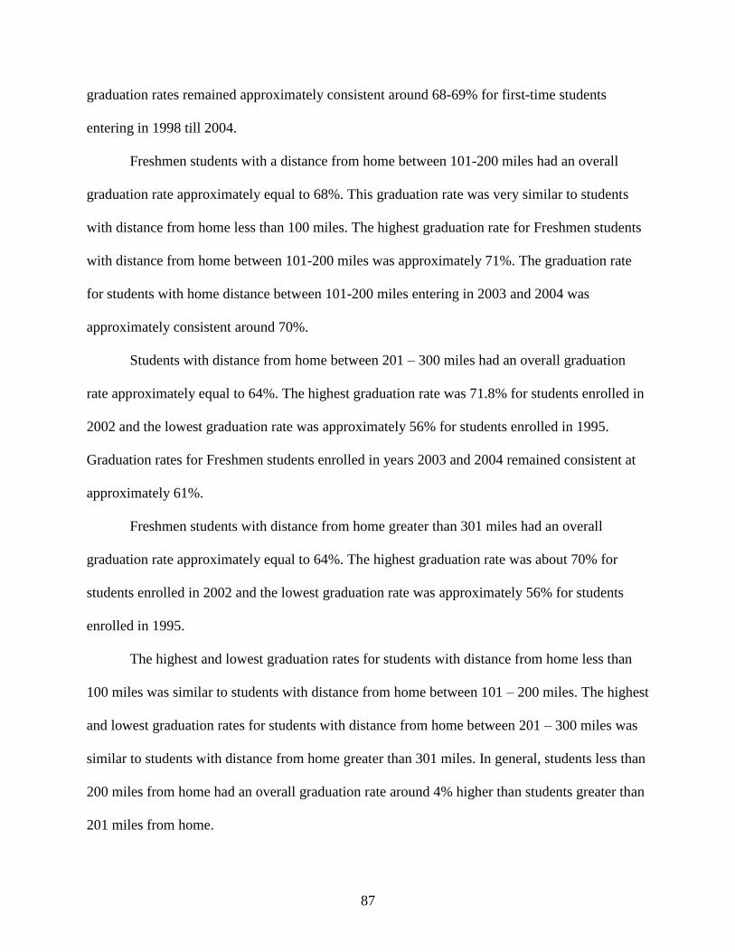
87
graduation rates remained approximately consistent around 68-69% for first-time students
entering in 1998 till 2004.
Freshmen students with a distance from home between 101-200 miles had an overall
graduation rate approximately equal to 68%. This graduation rate was very similar to students
with distance from home less than 100 miles. The highest graduation rate for Freshmen students
with distance from home between 101-200 miles was approximately 71%. The graduation rate
for students with home distance between 101-200 miles entering in 2003 and 2004 was
approximately consistent around 70%.
Students with distance from home between 201 – 300 miles had an overall graduation
rate approximately equal to 64%. The highest graduation rate was 71.8% for students enrolled in
2002 and the lowest graduation rate was approximately 56% for students enrolled in 1995.
Graduation rates for Freshmen students enrolled in years 2003 and 2004 remained consistent at
approximately 61%.
Freshmen students with distance from home greater than 301 miles had an overall
graduation rate approximately equal to 64%. The highest graduation rate was about 70% for
students enrolled in 2002 and the lowest graduation rate was approximately 56% for students
enrolled in 1995.
The highest and lowest graduation rates for students with distance from home less than
100 miles was similar to students with distance from home between 101 – 200 miles. The highest
and lowest graduation rates for students with distance from home between 201 – 300 miles was
similar to students with distance from home greater than 301 miles. In general, students less than
200 miles from home had an overall graduation rate around 4% higher than students greater than
201 miles from home.
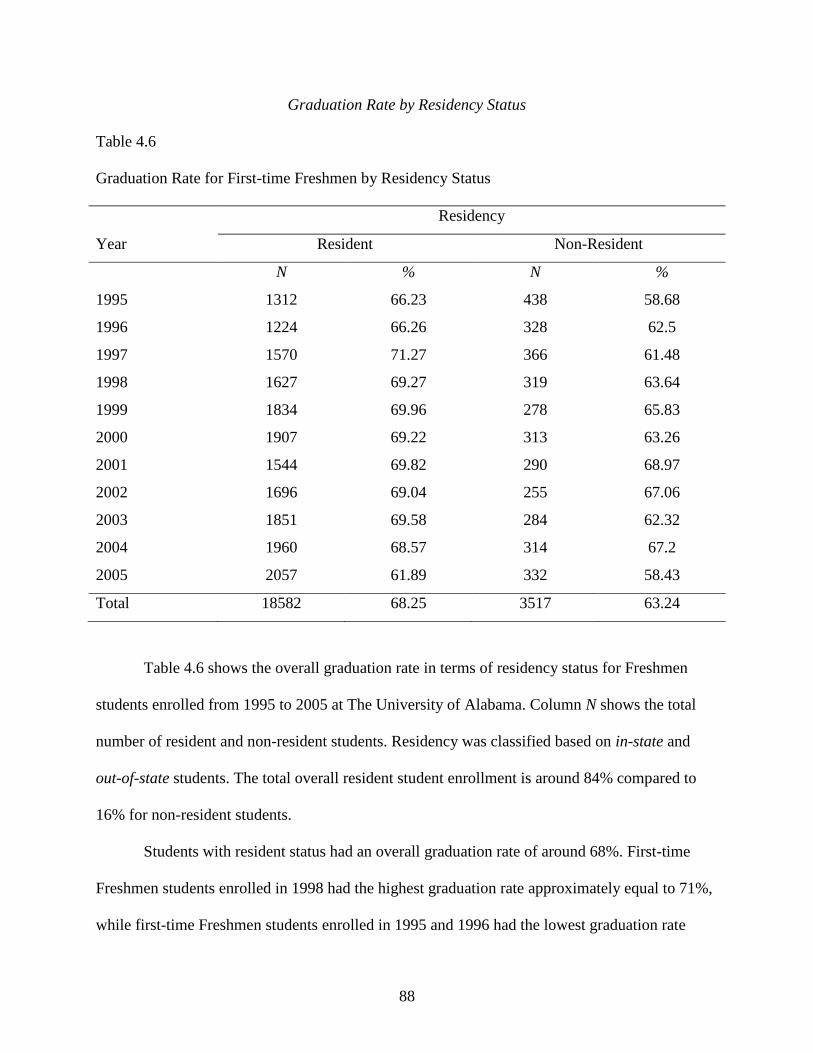
88
Graduation Rate by Residency Status
Table 4.6
Graduation Rate for First-time Freshmen by Residency Status
Residency
Year Resident Non-Resident
N % N %
1995 1312 66.23 438 58.68
1996 1224 66.26 328 62.5
1997 1570 71.27 366 61.48
1998 1627 69.27 319 63.64
1999 1834 69.96 278 65.83
2000 1907 69.22 313 63.26
2001 1544 69.82 290 68.97
2002 1696 69.04 255 67.06
2003 1851 69.58 284 62.32
2004 1960 68.57 314 67.2
2005 2057 61.89 332 58.43
Total 18582 68.25 3517 63.24
Table 4.6 shows the overall graduation rate in terms of residency status for Freshmen
students enrolled from 1995 to 2005 at The University of Alabama. Column N shows the total
number of resident and non-resident students. Residency was classified based on in-state and
out-of-state students. The total overall resident student enrollment is around 84% compared to
16% for non-resident students.
Students with resident status had an overall graduation rate of around 68%. First-time
Freshmen students enrolled in 1998 had the highest graduation rate approximately equal to 71%,
while first-time Freshmen students enrolled in 1995 and 1996 had the lowest graduation rate
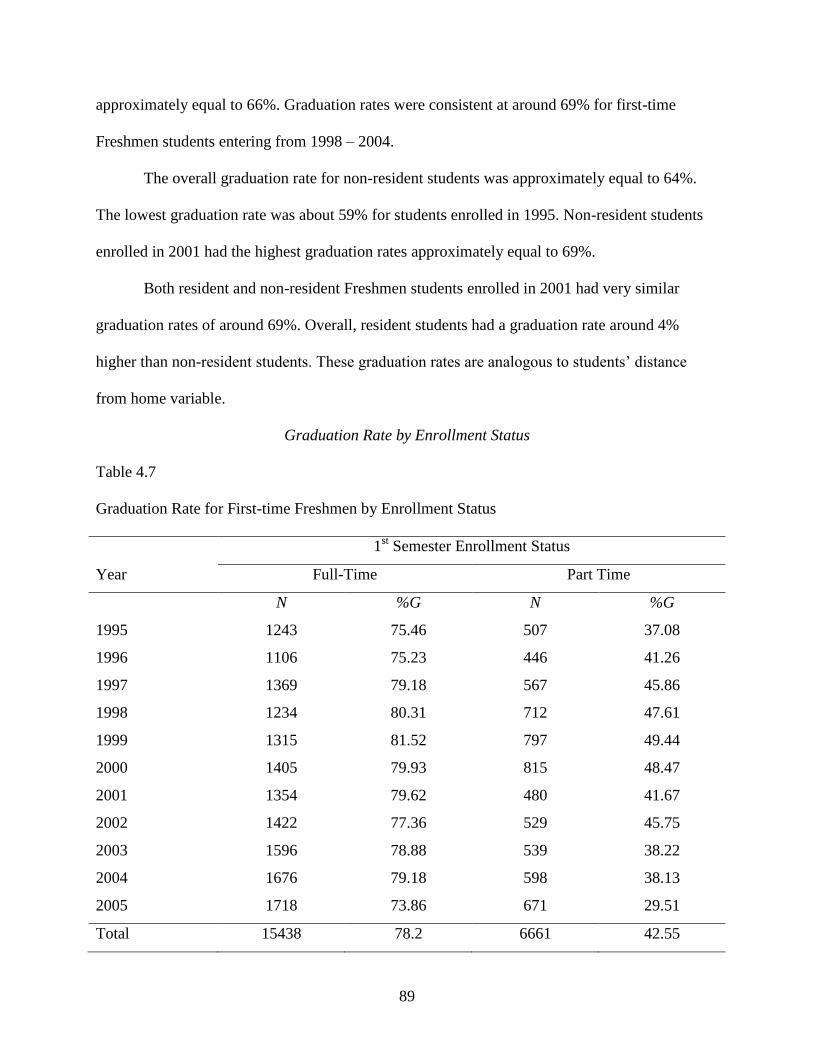
89
approximately equal to 66%. Graduation rates were consistent at around 69% for first-time
Freshmen students entering from 1998 – 2004.
The overall graduation rate for non-resident students was approximately equal to 64%.
The lowest graduation rate was about 59% for students enrolled in 1995. Non-resident students
enrolled in 2001 had the highest graduation rates approximately equal to 69%.
Both resident and non-resident Freshmen students enrolled in 2001 had very similar
graduation rates of around 69%. Overall, resident students had a graduation rate around 4%
higher than non-resident students. These graduation rates are analogous to students’ distance
from home variable.
Graduation Rate by Enrollment Status
Table 4.7
Graduation Rate for First-time Freshmen by Enrollment Status
1st Semester Enrollment Status
Year Full-Time Part Time
N %G N %G
1995 1243 75.46 507 37.08
1996 1106 75.23 446 41.26
1997 1369 79.18 567 45.86
1998 1234 80.31 712 47.61
1999 1315 81.52 797 49.44
2000 1405 79.93 815 48.47
2001 1354 79.62 480 41.67
2002 1422 77.36 529 45.75
2003 1596 78.88 539 38.22
2004 1676 79.18 598 38.13
2005 1718 73.86 671 29.51
Total 15438 78.2 6661 42.55
90
Table 4.7 shows the overall graduation rate in terms of first-semester enrollment status
for Freshmen students from 1995 to 2005 at The University of Alabama. Column N shows the
total number of full-time and part-time Freshmen students enrolled by year. Enrollment status
was classified based on 12 semester total earned hours at the end of first semester or not.
Students with less than 12 earned credit hours were classified as part-time students and students
greater than 12 earned credit hours were classified as full-time students. The total overall full
time students constitute around 70% compared to 30% for part-time students.
The overall graduation rate for full-time students was around 78%. The lowest graduation
rate for full-time students was around 75% for students enrolled in 1995 and 1996. Full-time
students enrolled in 1999 and 2000 had the highest graduation rates approximately equal to 81%.
Students with part-time status had an overall graduation rate of around 42%. First-time
Freshmen part-time students enrolled in 1995 had the highest graduation rate approximately
equal to 37%, while first-time Freshmen part-time students enrolled in 1999 had the lowest
graduation rate approximately equal to 50%. Graduation rates were consistently low at around
38% for first-time Freshmen part-time students entering in 2003 and 2004. On the whole, full-
time students had significantly higher graduation rates of around 36% compared to part-time
students.
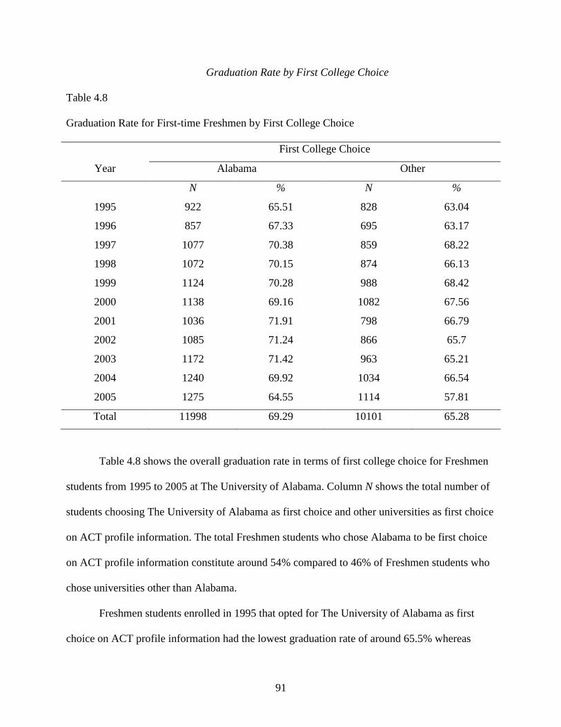
91
Graduation Rate by First College Choice
Table 4.8
Graduation Rate for First-time Freshmen by First College Choice
First College Choice
Year Alabama Other
N % N %
1995 922 65.51 828 63.04
1996 857 67.33 695 63.17
1997 1077 70.38 859 68.22
1998 1072 70.15 874 66.13
1999 1124 70.28 988 68.42
2000 1138 69.16 1082 67.56
2001 1036 71.91 798 66.79
2002 1085 71.24 866 65.7
2003 1172 71.42 963 65.21
2004 1240 69.92 1034 66.54
2005 1275 64.55 1114 57.81
Total 11998 69.29 10101 65.28
Table 4.8 shows the overall graduation rate in terms of first college choice for Freshmen
students from 1995 to 2005 at The University of Alabama. Column N shows the total number of
students choosing The University of Alabama as first choice and other universities as first choice
on ACT profile information. The total Freshmen students who chose Alabama to be first choice
on ACT profile information constitute around 54% compared to 46% of Freshmen students who
chose universities other than Alabama.
Freshmen students enrolled in 1995 that opted for The University of Alabama as first
choice on ACT profile information had the lowest graduation rate of around 65.5% whereas
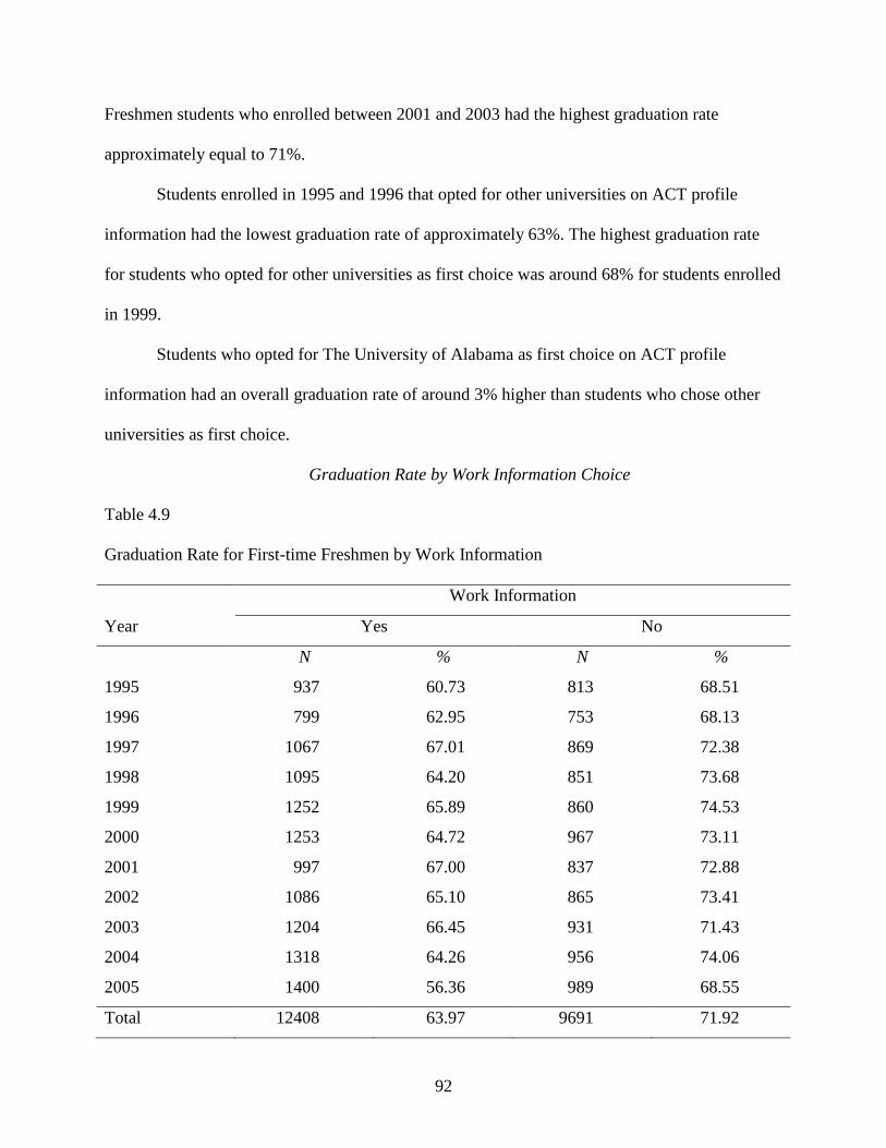
92
Freshmen students who enrolled between 2001 and 2003 had the highest graduation rate
approximately equal to 71%.
Students enrolled in 1995 and 1996 that opted for other universities on ACT profile
information had the lowest graduation rate of approximately 63%. The highest graduation rate
for students who opted for other universities as first choice was around 68% for students enrolled
in 1999.
Students who opted for The University of Alabama as first choice on ACT profile
information had an overall graduation rate of around 3% higher than students who chose other
universities as first choice.
Graduation Rate by Work Information Choice
Table 4.9
Graduation Rate for First-time Freshmen by Work Information
Work Information
Year Yes No
N % N %
1995 937 60.73 813 68.51
1996 799 62.95 753 68.13
1997 1067 67.01 869 72.38
1998 1095 64.20 851 73.68
1999 1252 65.89 860 74.53
2000 1253 64.72 967 73.11
2001 997 67.00 837 72.88
2002 1086 65.10 865 73.41
2003 1204 66.45 931 71.43
2004 1318 64.26 956 74.06
2005 1400 56.36 989 68.55
Total 12408 63.97 9691 71.92
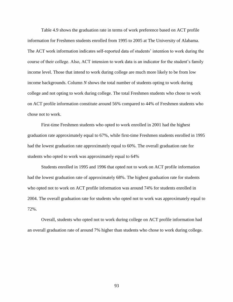
93
Table 4.9 shows the graduation rate in terms of work preference based on ACT profile
information for Freshmen students enrolled from 1995 to 2005 at The University of Alabama.
The ACT work information indicates self-reported data of students’ intention to work during the
course of their college. Also, ACT intension to work data is an indicator for the student’s family
income level. Those that intend to work during college are much more likely to be from low
income backgrounds. Column N shows the total number of students opting to work during
college and not opting to work during college. The total Freshmen students who chose to work
on ACT profile information constitute around 56% compared to 44% of Freshmen students who
chose not to work.
First-time Freshmen students who opted to work enrolled in 2001 had the highest
graduation rate approximately equal to 67%, while first-time Freshmen students enrolled in 1995
had the lowest graduation rate approximately equal to 60%. The overall graduation rate for
students who opted to work was approximately equal to 64%
Students enrolled in 1995 and 1996 that opted not to work on ACT profile information
had the lowest graduation rate of approximately 68%. The highest graduation rate for students
who opted not to work on ACT profile information was around 74% for students enrolled in
2004. The overall graduation rate for students who opted not to work was approximately equal to
72%.
Overall, students who opted not to work during college on ACT profile information had
an overall graduation rate of around 7% higher than students who chose to work during college.

94
Graduation Rate by Advanced Placement Credit
Table 4.10
Graduation Rate for First-time Freshmen by Advanced Placement Credit
Advanced Placement Credit
Year Yes No
N % N %
1995 187 80.75 1563 62.38
1996 249 78.71 1303 62.93
1997 256 85.55 1680 66.96
1998 223 83.86 1723 66.34
1999 255 90.98 1857 66.45
2000 254 83.07 1966 66.48
2001 219 89.04 1615 67.06
2002 215 88.37 1736 66.36
2003 244 84.02 1891 66.63
2004 293 83.28 1981 66.18
2005 383 80.42 2006 57.78
Total 2778 84.16 19321 65.05
Table 4.10 shows the graduation rate in terms of advanced placement credit hours for
Freshmen students enrolled from 1995 to 2005 at The University of Alabama. Column N shows
the total number of students having advanced placement credit hours and students not having any
advanced placement credit hours. The total Freshmen students having advanced placement credit
was approximately 10% compared to 90% of Freshmen students with no advanced placement
credit hours.
Freshmen students entering with advanced placement credit hours in 1999 had the highest
graduation rate approximately equal to 90%. The lowest graduation rate was around 79% for
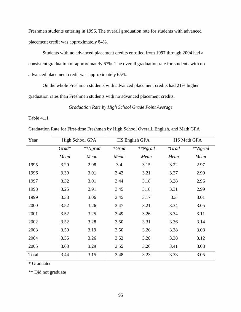
95
Freshmen students entering in 1996. The overall graduation rate for students with advanced
placement credit was approximately 84%.
Students with no advanced placement credits enrolled from 1997 through 2004 had a
consistent graduation of approximately 67%. The overall graduation rate for students with no
advanced placement credit was approximately 65%.
On the whole Freshmen students with advanced placement credits had 21% higher
graduation rates than Freshmen students with no advanced placement credits.
Graduation Rate by High School Grade Point Average
Table 4.11
Graduation Rate for First-time Freshmen by High School Overall, English, and Math GPA
Year High School GPA HS English GPA HS Math GPA
Grad*
Mean
**Ngrad
Mean
*Grad
Mean
**Ngrad
Mean
*Grad
Mean
**Ngrad
Mean
1995 3.29 2.98 3.4 3.15 3.22 2.97
1996 3.30 3.01 3.42 3.21 3.27 2.99
1997 3.32 3.01 3.44 3.18 3.28 2.96
1998 3.25 2.91 3.45 3.18 3.31 2.99
1999 3.38 3.06 3.45 3.17 3.3 3.01
2000 3.52 3.26 3.47 3.21 3.34 3.05
2001 3.52 3.25 3.49 3.26 3.34 3.11
2002 3.52 3.28 3.50 3.31 3.36 3.14
2003 3.50 3.19 3.50 3.26 3.38 3.08
2004 3.55 3.26 3.52 3.28 3.38 3.12
2005 3.63 3.29 3.55 3.26 3.41 3.08
Total 3.44 3.15 3.48 3.23 3.33 3.05
* Graduated
** Did not graduate

96
Table 4.11 shows the overall high school grade point average, high school English GPA,
and high school math GPA of Freshmen students enrolled from 1995 to 2005 at The University
of Alabama. Column “*Grad mean” shows the high school grade point average of students who
graduated and column “**Ngrad mean” mean shows the high school grade point average of
students who did not graduate from the University of Alabama.
Graduated students enrolled in 1998 had the lowest grade point average of 3.25 and
graduated students enrolled in 2005 had the highest grade point average of 3.63. High school
grade point average for graduated students was consistent around 3.5 for graduated students from
2000-2004. Leaving students enrolled in 1995 had the lowest grade point average of 2.98 and
non-graduate students enrolled in 2005 had the highest grade point average of 3.29. Overall high
school grade point average for graduated students was 3.44 and high school grade point average
for leaving students was 3.15.
High school English GPA for graduated students was consistent between 3.4 and 3.5,
while the overall average GPA was 3.48. Overall English GPA for non-graduate students was
3.23.
Overall high school math GPA for graduated students was 3.05. High school math GPA
was relatively lower than high school English GPA and cumulative high school GPA.
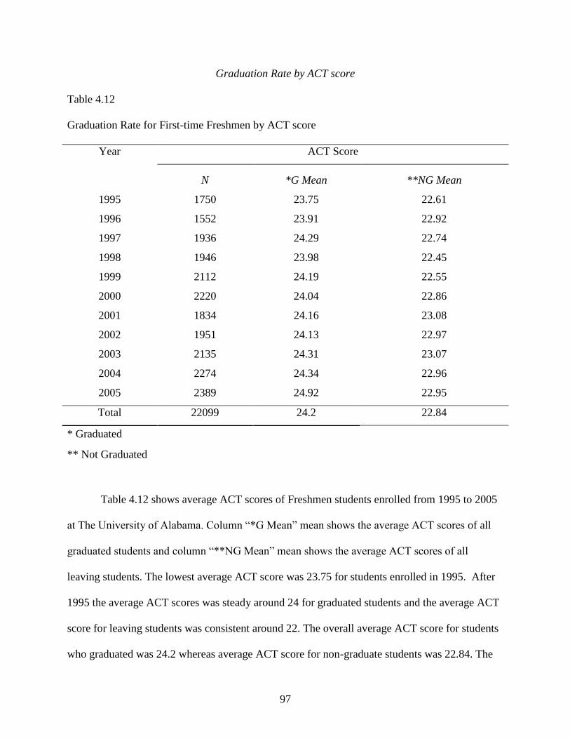
97
Graduation Rate by ACT score
Table 4.12
Graduation Rate for First-time Freshmen by ACT score
Year ACT Score
N *G Mean **NG Mean
1995 1750 23.75 22.61
1996 1552 23.91 22.92
1997 1936 24.29 22.74
1998 1946 23.98 22.45
1999 2112 24.19 22.55
2000 2220 24.04 22.86
2001 1834 24.16 23.08
2002 1951 24.13 22.97
2003 2135 24.31 23.07
2004 2274 24.34 22.96
2005 2389 24.92 22.95
Total 22099 24.2 22.84
* Graduated
** Not Graduated
Table 4.12 shows average ACT scores of Freshmen students enrolled from 1995 to 2005
at The University of Alabama. Column “*G Mean” mean shows the average ACT scores of all
graduated students and column “**NG Mean” mean shows the average ACT scores of all
leaving students. The lowest average ACT score was 23.75 for students enrolled in 1995. After
1995 the average ACT scores was steady around 24 for graduated students and the average ACT
score for leaving students was consistent around 22. The overall average ACT score for students
who graduated was 24.2 whereas average ACT score for non-graduate students was 22.84. The
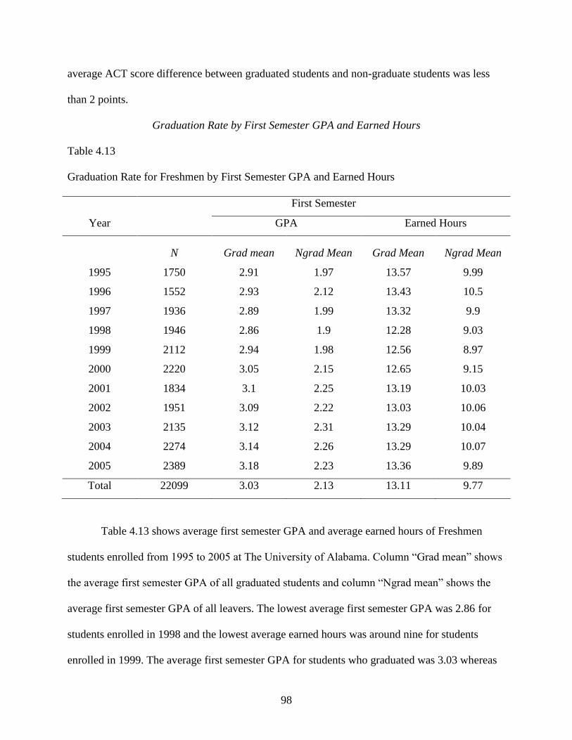
98
average ACT score difference between graduated students and non-graduate students was less
than 2 points.
Graduation Rate by First Semester GPA and Earned Hours
Table 4.13
Graduation Rate for Freshmen by First Semester GPA and Earned Hours
First Semester
Year GPA Earned Hours
N Grad mean Ngrad Mean Grad Mean Ngrad Mean
1995 1750 2.91 1.97 13.57 9.99
1996 1552 2.93 2.12 13.43 10.5
1997 1936 2.89 1.99 13.32 9.9
1998 1946 2.86 1.9 12.28 9.03
1999 2112 2.94 1.98 12.56 8.97
2000 2220 3.05 2.15 12.65 9.15
2001 1834 3.1 2.25 13.19 10.03
2002 1951 3.09 2.22 13.03 10.06
2003 2135 3.12 2.31 13.29 10.04
2004 2274 3.14 2.26 13.29 10.07
2005 2389 3.18 2.23 13.36 9.89
Total 22099 3.03 2.13 13.11 9.77
Table 4.13 shows average first semester GPA and average earned hours of Freshmen
students enrolled from 1995 to 2005 at The University of Alabama. Column “Grad mean” shows
the average first semester GPA of all graduated students and column “Ngrad mean” shows the
average first semester GPA of all leavers. The lowest average first semester GPA was 2.86 for
students enrolled in 1998 and the lowest average earned hours was around nine for students
enrolled in 1999. The average first semester GPA for students who graduated was 3.03 whereas
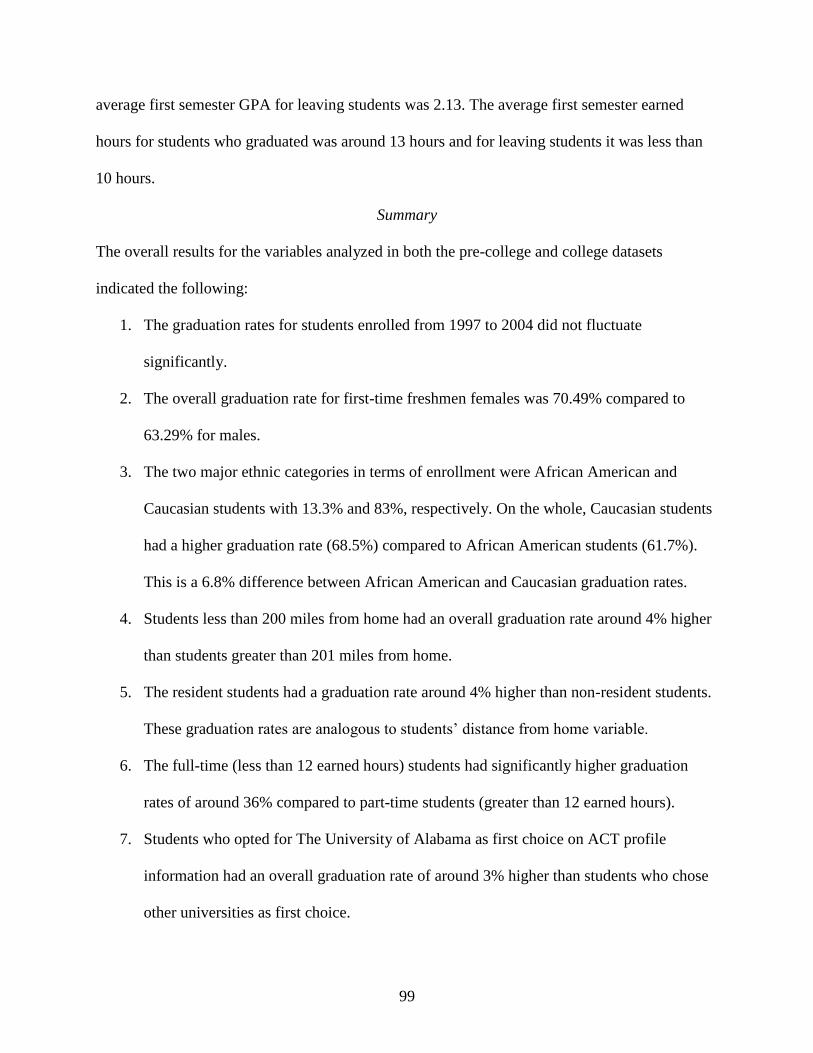
99
average first semester GPA for leaving students was 2.13. The average first semester earned
hours for students who graduated was around 13 hours and for leaving students it was less than
10 hours.
Summary
The overall results for the variables analyzed in both the pre-college and college datasets
indicated the following:
1. The graduation rates for students enrolled from 1997 to 2004 did not fluctuate
significantly.
2. The overall graduation rate for first-time freshmen females was 70.49% compared to
63.29% for males.
3. The two major ethnic categories in terms of enrollment were African American and
Caucasian students with 13.3% and 83%, respectively. On the whole, Caucasian students
had a higher graduation rate (68.5%) compared to African American students (61.7%).
This is a 6.8% difference between African American and Caucasian graduation rates.
4. Students less than 200 miles from home had an overall graduation rate around 4% higher
than students greater than 201 miles from home.
5. The resident students had a graduation rate around 4% higher than non-resident students.
These graduation rates are analogous to students’ distance from home variable.
6. The full-time (less than 12 earned hours) students had significantly higher graduation
rates of around 36% compared to part-time students (greater than 12 earned hours).
7. Students who opted for The University of Alabama as first choice on ACT profile
information had an overall graduation rate of around 3% higher than students who chose
other universities as first choice.
100
8. Students who expected not to work during college on ACT profile information had an
overall graduation rate of around 7% higher than students who expected to work during
college.
9. Freshmen students with advanced placement credits had 21% higher graduation rates
than Freshmen students with no advanced placement credits.
10. The high school math GPA for graduated students was 3.05. High school math GPA was
relatively lower than high school English GPA and cumulative high school GPA.
11. The average first semester earned hours for students who graduated was around 13 hours
and for leaving students it was less than 10 hours.
Outliers and Missing Values
Extracted data from The University of Alabama’s enterprise resource planning system
(ERP) were merged with ACT data based on the unique identification number. List-wise deletion
method deleted the entire record from the analyses if a single observation of any variable was
missing. Outlier analysis for categorical variables was done using frequency tables; any invalid
categories within the variables were deleted. Outlier analysis for continuous variables was
performed using SAS® JMP software. Mahalanobis distance was used to delete the outliers (see
Figure 4.2). Variance Inflation Factors (VIFs) did not identify the presence of any multi-
collinearity, amongst the variables. After performing list-wise deletion and outlier analysis, there
were 22,099 total observations in the dataset.
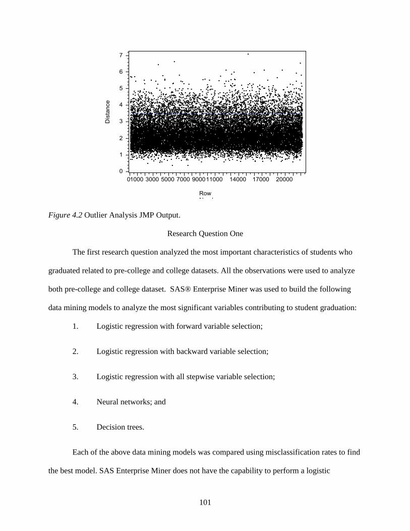
101
Figure 4.2 Outlier Analysis JMP Output.
Research Question One
The first research question analyzed the most important characteristics of students who
graduated related to pre-college and college datasets. All the observations were used to analyze
both pre-college and college dataset. SAS® Enterprise Miner was used to build the following
data mining models to analyze the most significant variables contributing to student graduation:
1. Logistic regression with forward variable selection;
2. Logistic regression with backward variable selection;
3. Logistic regression with all stepwise variable selection;
4. Neural networks; and
5. Decision trees.
Each of the above data mining models was compared using misclassification rates to find
the best model. SAS Enterprise Miner does not have the capability to perform a logistic
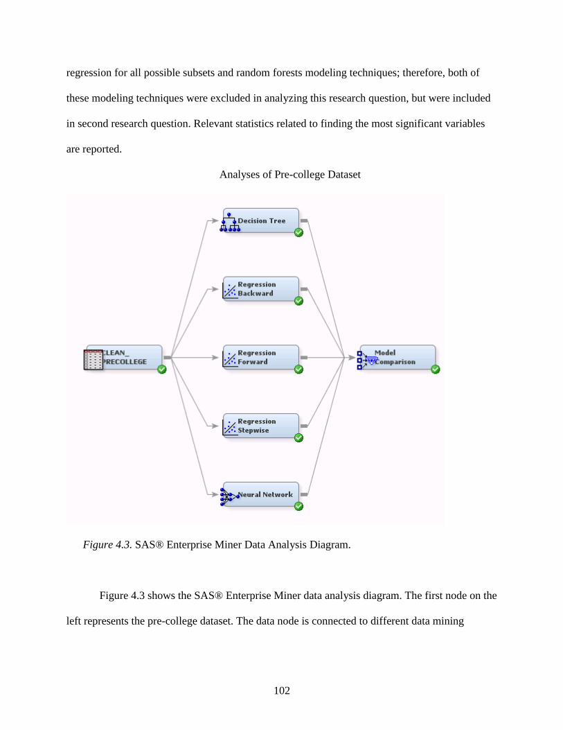
102
regression for all possible subsets and random forests modeling techniques; therefore, both of
these modeling techniques were excluded in analyzing this research question, but were included
in second research question. Relevant statistics related to finding the most significant variables
are reported.
Analyses of Pre-college Dataset
Figure 4.3. SAS® Enterprise Miner Data Analysis Diagram.
Figure 4.3 shows the SAS® Enterprise Miner data analysis diagram. The first node on the
left represents the pre-college dataset. The data node is connected to different data mining
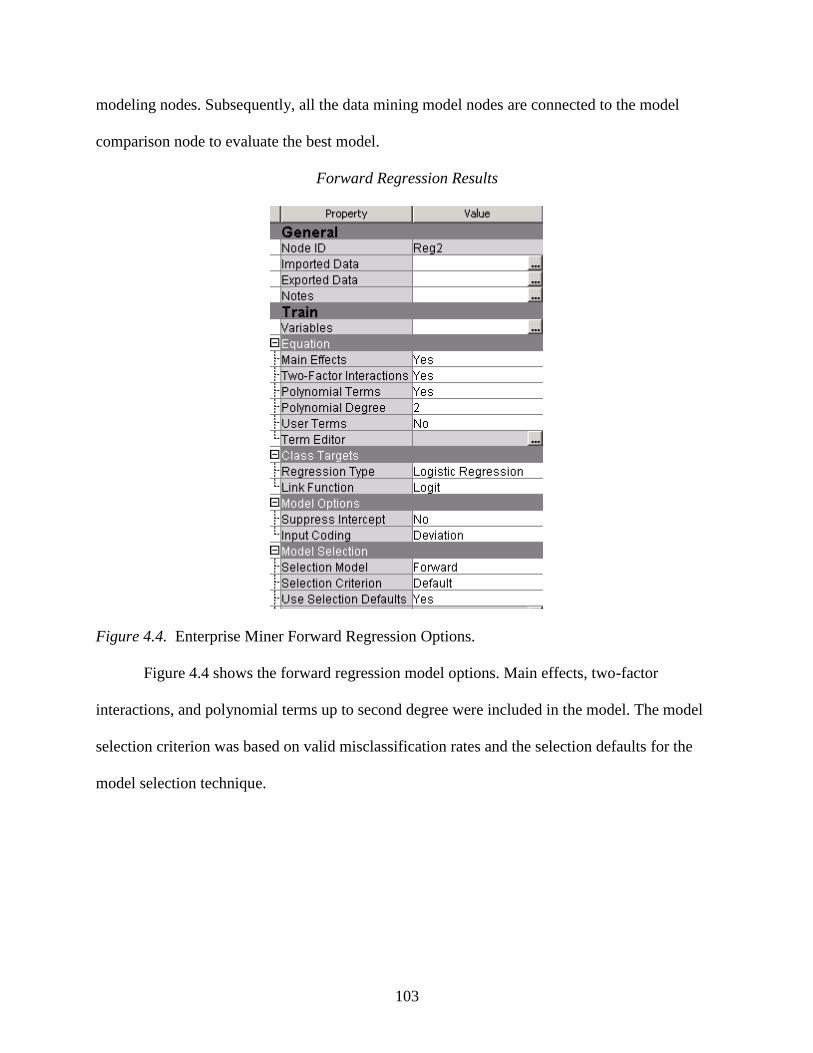
103
modeling nodes. Subsequently, all the data mining model nodes are connected to the model
comparison node to evaluate the best model.
Forward Regression Results
Figure 4.4. Enterprise Miner Forward Regression Options.
Figure 4.4 shows the forward regression model options. Main effects, two-factor
interactions, and polynomial terms up to second degree were included in the model. The model
selection criterion was based on valid misclassification rates and the selection defaults for the
model selection technique.
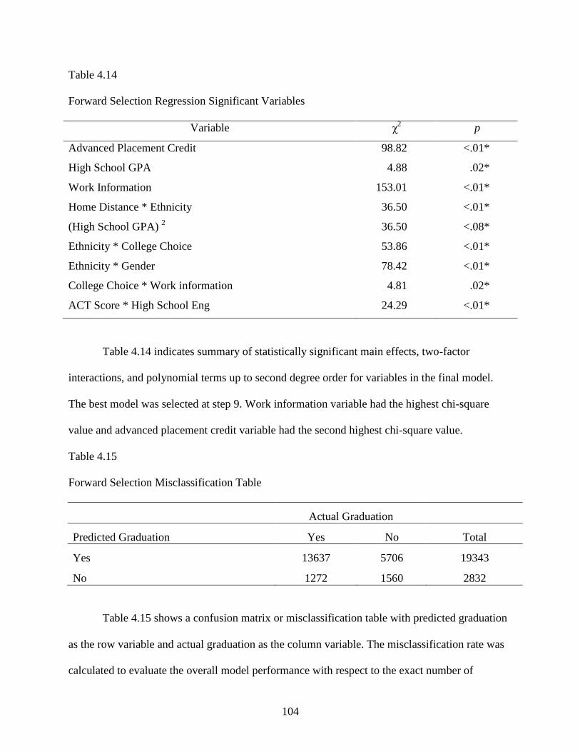
104
Table 4.14
Forward Selection Regression Significant Variables
Variable χ2 p
Advanced Placement Credit 98.82 <.01*
High School GPA 4.88 .02*
Work Information 153.01 <.01*
Home Distance * Ethnicity 36.50 <.01*
(High School GPA) 2 36.50 <.08*
Ethnicity * College Choice 53.86 <.01*
Ethnicity * Gender 78.42 <.01*
College Choice * Work information 4.81 .02*
ACT Score * High School Eng 24.29 <.01*
Table 4.14 indicates summary of statistically significant main effects, two-factor
interactions, and polynomial terms up to second degree order for variables in the final model.
The best model was selected at step 9. Work information variable had the highest chi-square
value and advanced placement credit variable had the second highest chi-square value.
Table 4.15
Forward Selection Misclassification Table
Actual Graduation
Predicted Graduation Yes No Total
Yes 13637 5706 19343
No 1272 1560 2832
Table 4.15 shows a confusion matrix or misclassification table with predicted graduation
as the row variable and actual graduation as the column variable. The misclassification rate was
calculated to evaluate the overall model performance with respect to the exact number of
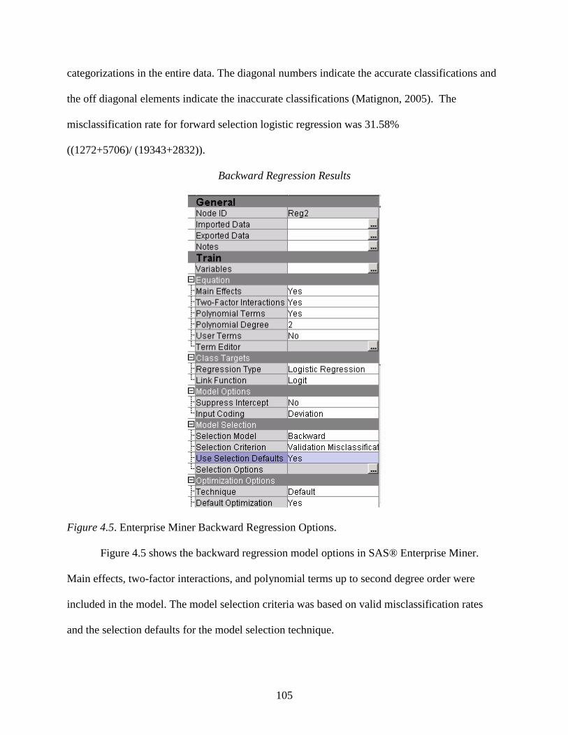
105
categorizations in the entire data. The diagonal numbers indicate the accurate classifications and
the off diagonal elements indicate the inaccurate classifications (Matignon, 2005). The
misclassification rate for forward selection logistic regression was 31.58%
((1272+5706)/ (19343+2832)).
Backward Regression Results
Figure 4.5. Enterprise Miner Backward Regression Options.
Figure 4.5 shows the backward regression model options in SAS® Enterprise Miner.
Main effects, two-factor interactions, and polynomial terms up to second degree order were
included in the model. The model selection criteria was based on valid misclassification rates
and the selection defaults for the model selection technique.
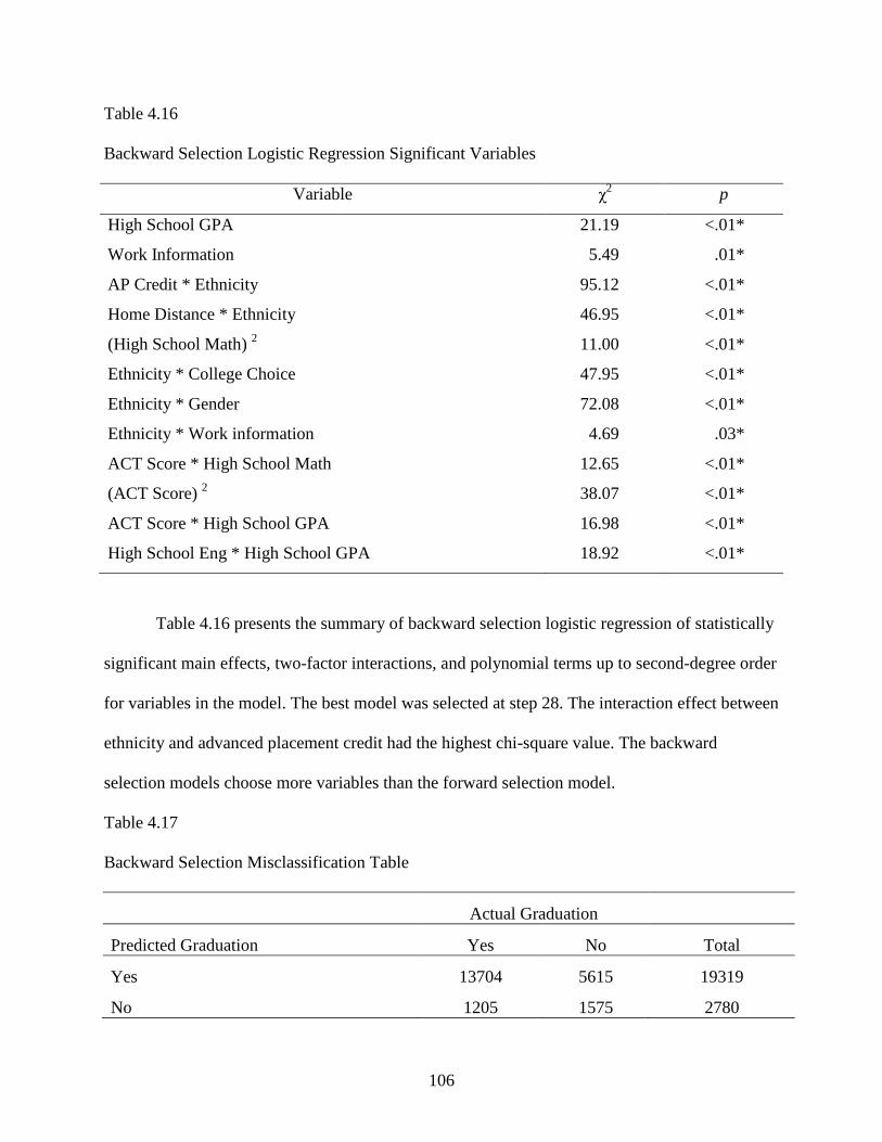
106
Table 4.16
Backward Selection Logistic Regression Significant Variables
Variable χ2 p
High School GPA 21.19 <.01*
Work Information 5.49 .01*
AP Credit * Ethnicity 95.12 <.01*
Home Distance * Ethnicity 46.95 <.01*
(High School Math) 2 11.00 <.01*
Ethnicity * College Choice 47.95 <.01*
Ethnicity * Gender 72.08 <.01*
Ethnicity * Work information 4.69 .03*
ACT Score * High School Math 12.65 <.01*
(ACT Score) 2 38.07 <.01*
ACT Score * High School GPA 16.98 <.01*
High School Eng * High School GPA 18.92 <.01*
Table 4.16 presents the summary of backward selection logistic regression of statistically
significant main effects, two-factor interactions, and polynomial terms up to second-degree order
for variables in the model. The best model was selected at step 28. The interaction effect between
ethnicity and advanced placement credit had the highest chi-square value. The backward
selection models choose more variables than the forward selection model.
Table 4.17
Backward Selection Misclassification Table
Actual Graduation
Predicted Graduation Yes No Total
Yes 13704 5615 19319
No 1205 1575 2780
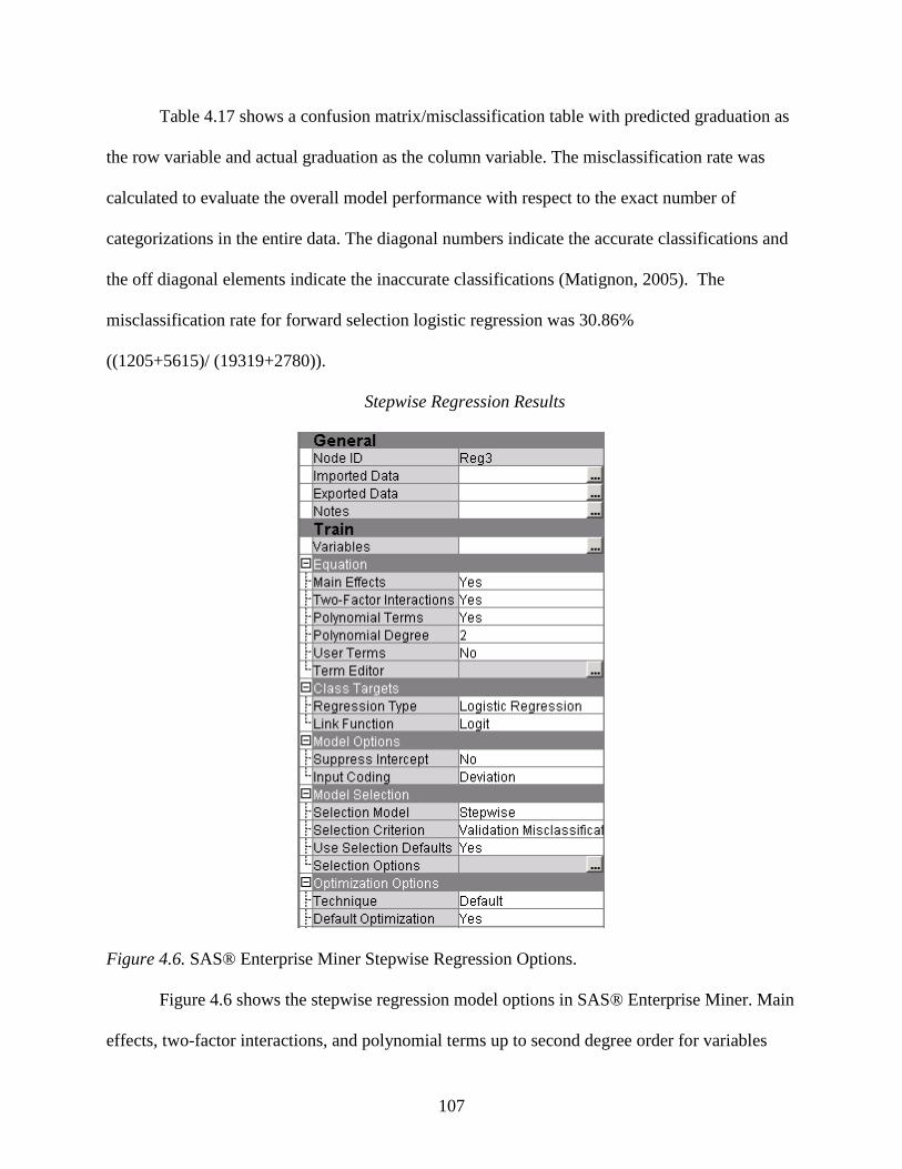
107
Table 4.17 shows a confusion matrix/misclassification table with predicted graduation as
the row variable and actual graduation as the column variable. The misclassification rate was
calculated to evaluate the overall model performance with respect to the exact number of
categorizations in the entire data. The diagonal numbers indicate the accurate classifications and
the off diagonal elements indicate the inaccurate classifications (Matignon, 2005). The
misclassification rate for forward selection logistic regression was 30.86%
((1205+5615)/ (19319+2780)).
Stepwise Regression Results
Figure 4.6. SAS® Enterprise Miner Stepwise Regression Options.
Figure 4.6 shows the stepwise regression model options in SAS® Enterprise Miner. Main
effects, two-factor interactions, and polynomial terms up to second degree order for variables
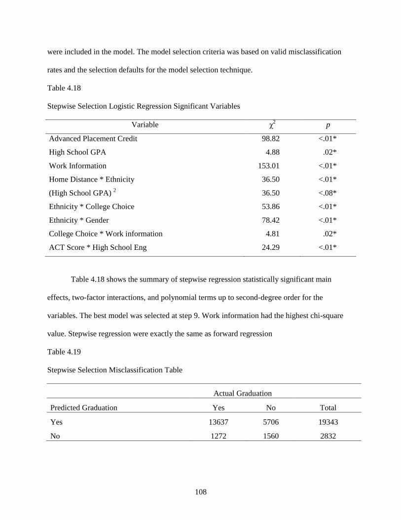
108
were included in the model. The model selection criteria was based on valid misclassification
rates and the selection defaults for the model selection technique.
Table 4.18
Stepwise Selection Logistic Regression Significant Variables
Variable χ2 p
Advanced Placement Credit 98.82 <.01*
High School GPA 4.88 .02*
Work Information 153.01 <.01*
Home Distance * Ethnicity 36.50 <.01*
(High School GPA) 2 36.50 <.08*
Ethnicity * College Choice 53.86 <.01*
Ethnicity * Gender 78.42 <.01*
College Choice * Work information 4.81 .02*
ACT Score * High School Eng 24.29 <.01*
Table 4.18 shows the summary of stepwise regression statistically significant main
effects, two-factor interactions, and polynomial terms up to second-degree order for the
variables. The best model was selected at step 9. Work information had the highest chi-square
value. Stepwise regression were exactly the same as forward regression
Table 4.19
Stepwise Selection Misclassification Table
Actual Graduation
Predicted Graduation Yes No Total
Yes 13637 5706 19343
No 1272 1560 2832
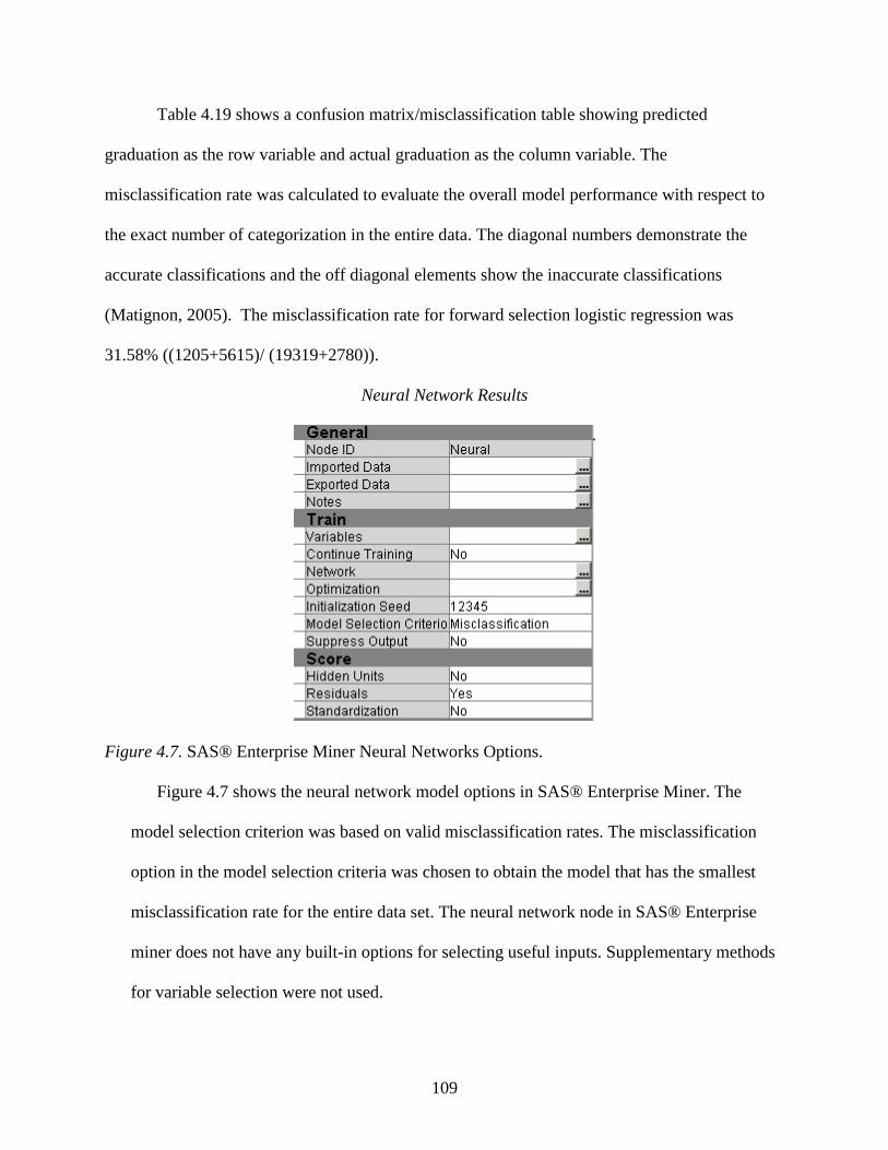
109
Table 4.19 shows a confusion matrix/misclassification table showing predicted
graduation as the row variable and actual graduation as the column variable. The
misclassification rate was calculated to evaluate the overall model performance with respect to
the exact number of categorization in the entire data. The diagonal numbers demonstrate the
accurate classifications and the off diagonal elements show the inaccurate classifications
(Matignon, 2005). The misclassification rate for forward selection logistic regression was
31.58% ((1205+5615)/ (19319+2780)).
Neural Network Results
Figure 4.7. SAS® Enterprise Miner Neural Networks Options.
Figure 4.7 shows the neural network model options in SAS® Enterprise Miner. The
model selection criterion was based on valid misclassification rates. The misclassification
option in the model selection criteria was chosen to obtain the model that has the smallest
misclassification rate for the entire data set. The neural network node in SAS® Enterprise
miner does not have any built-in options for selecting useful inputs. Supplementary methods
for variable selection were not used.
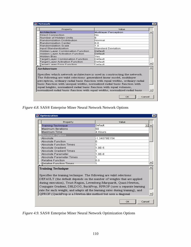
110
Figure 4.8. SAS® Enterprise Miner Neural Network Network Options
Figure 4.9. SAS® Enterprise Miner Neural Network Optimization Options

111
Figure 4.8 shows the stopped training network options for the neural network model. A
multilayer model was used as network architecture in constructing the neural network model.
The default option for the number of hidden layers is three; however, the default number of three
hidden layers does not always give the optimal model. SAS recommends using six different
hidden units (Georges, 2008). A normal distribution was used as the randomization distribution
to apply to the weights. The standard deviation was selected to standardize the input variables
into the network. The default option was selected for both hidden layer combination function and
hidden layer activation functions. The default activation technique depends on the number of
weights that are applied during execution. A maximum of 50 iterations and four hours of
maximum time were used.
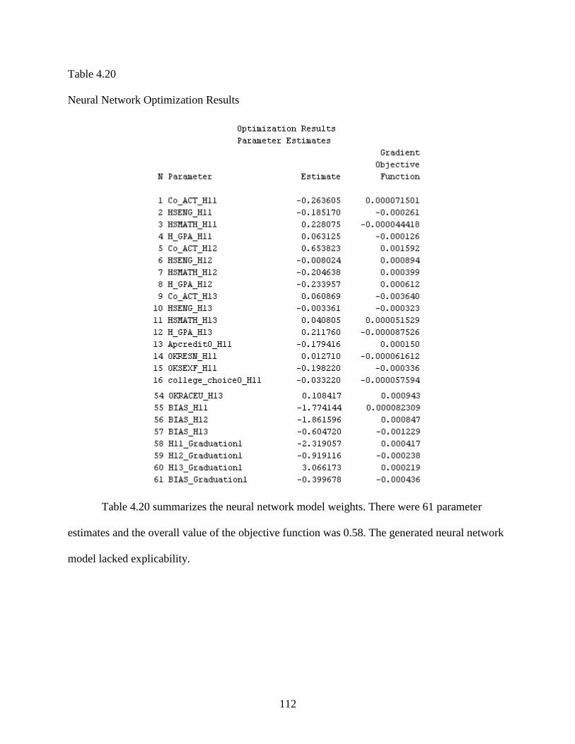
112
Table 4.20
Neural Network Optimization Results
Table 4.20 summarizes the neural network model weights. There were 61 parameter
estimates and the overall value of the objective function was 0.58. The generated neural network
model lacked explicability.

113
Table 4.21
Neural Network Model Misclassification Table
Actual Graduation
Predicted Graduation Yes No Total
Yes 13730 5836 19566
No 1103 1430 2533
Table 4.21 shows the confusion matrix or misclassification table with predicted
graduation as the row variable and actual graduation as the column variable. The
misclassification rate was calculated to evaluate the overall model performance with respect to
the exact number of categorizations in the entire data. The diagonal numbers indicate the
accurate classifications and the off diagonal elements indicate the inaccurate classifications
(Matignon, 2005). The misclassification rate for the neural network model was close to 31%
((1103+5836)/(19566+2533)).
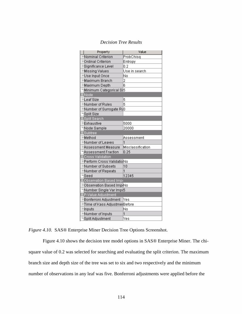
114
Decision Tree Results
Figure 4.10. SAS® Enterprise Miner Decision Tree Options Screenshot.
Figure 4.10 shows the decision tree model options in SAS® Enterprise Miner. The chi-
square value of 0.2 was selected for searching and evaluating the split criterion. The maximum
branch size and depth size of the tree was set to six and two respectively and the minimum
number of observations in any leaf was five. Bonferroni adjustments were applied before the

115
split was chosen. The model selection criterion was based on valid misclassification rates. The
misclassification option in the model selection criteria chooses the model that has the smallest
misclassification rate for the entire dataset.
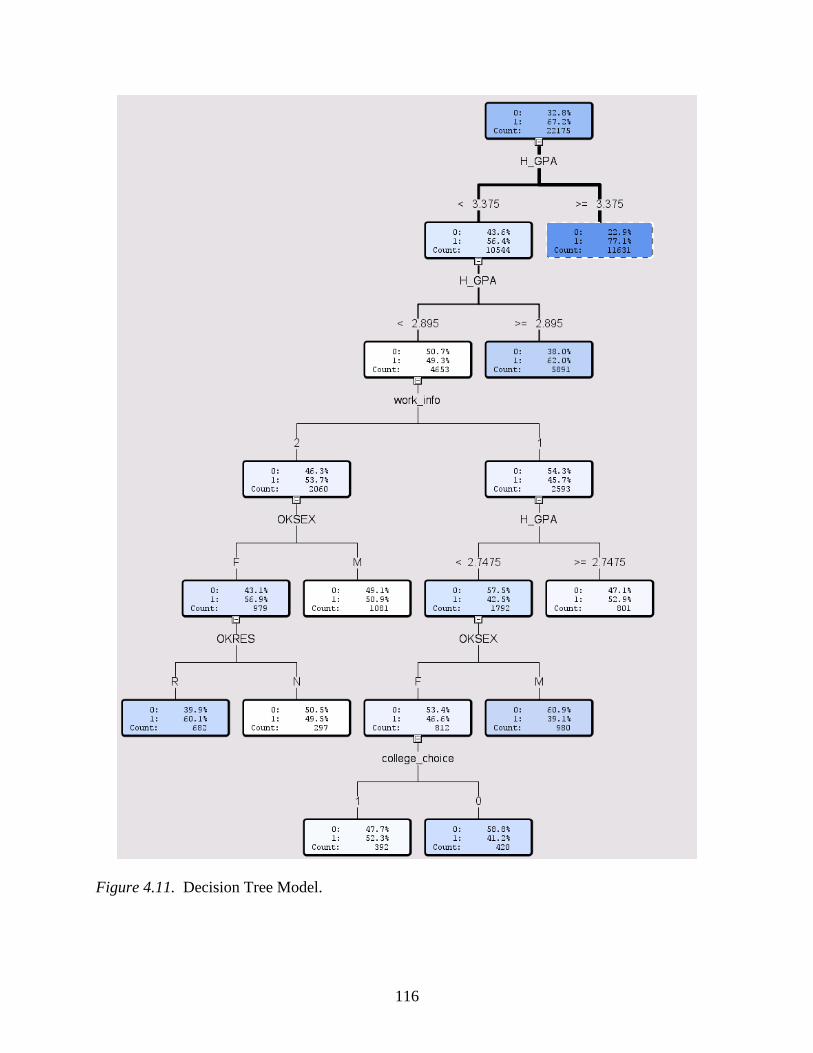
116
Figure 4.11. Decision Tree Model.
117
Figure 4.11 shows the generated decision tree model. Data was first split based on high
school GPA. The first branch on the top right contains cases with high school GPA greater than
or equal to 3.375 and the second branch on the top left contains cases with first-year GPA less
than 3.375.
The right branch top node with high school GPA greater than or equal to 3.375 had
11,631 cases. 77.1% out of 11631 students with high school GPA greater than 3.375 graduated
and 22.9% did not graduate. The first path was the most significant path.
The left branch top node with high school GPA less than 3.375 had 10,544 cases. 56.4%
of 10,544 students with high school GPA less than 3.375 graduated. This node was further
broken down into students with high school GPA less than 2.89 and high school GPA greater
than 2.89. The node for first-year GPA less than 2.89 was further divided based on work
information.
The 53.7% of 2060 students with work information ‘yes’ graduated and 45.7% of 2593
students with work information ‘no’ graduated. Work information ‘yes’ node was further
divided based on gender. The 56.9% female students out of 979 graduated, whereas 50.9% male
students out of 1081 graduated. The female gender node was further divided based on residency
status. The 60.1% out of 682 female resident students graduated whereas 49.5% of 297 female
non- resident students graduated.
Work information ‘no’ node was further broken down into students with high school
GPA less than 2.74 and high school GPA greater than or equal to 2.74. The 52.9% out of 801
students with high school GPA greater than or equal to 2.74 graduated whereas 42.5% out of
1792 students with high school GPA less than 2.74 graduated. High school GPA less than 2.74
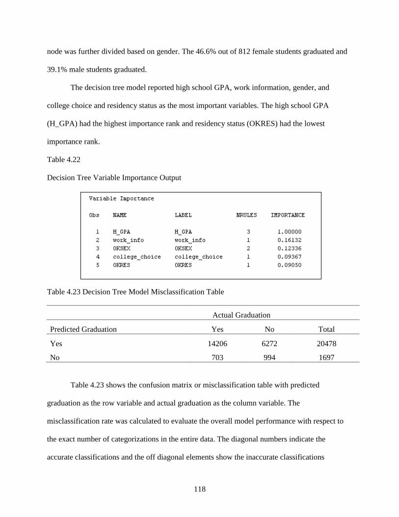
118
node was further divided based on gender. The 46.6% out of 812 female students graduated and
39.1% male students graduated.
The decision tree model reported high school GPA, work information, gender, and
college choice and residency status as the most important variables. The high school GPA
(H_GPA) had the highest importance rank and residency status (OKRES) had the lowest
importance rank.
Table 4.22
Decision Tree Variable Importance Output
Table 4.23 Decision Tree Model Misclassification Table
Actual Graduation
Predicted Graduation Yes No Total
Yes 14206 6272 20478
No 703 994 1697
Table 4.23 shows the confusion matrix or misclassification table with predicted
graduation as the row variable and actual graduation as the column variable. The
misclassification rate was calculated to evaluate the overall model performance with respect to
the exact number of categorizations in the entire data. The diagonal numbers indicate the
accurate classifications and the off diagonal elements show the inaccurate classifications
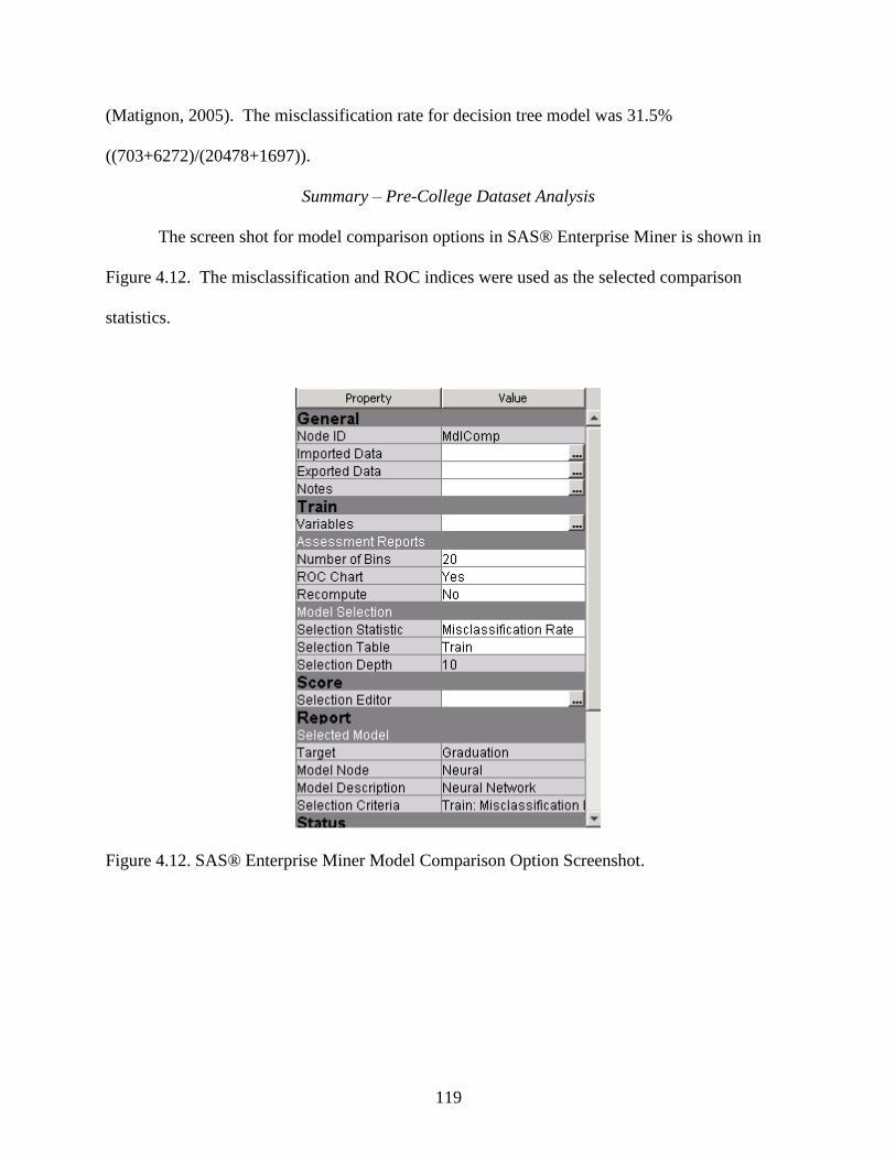
119
(Matignon, 2005). The misclassification rate for decision tree model was 31.5%
((703+6272)/(20478+1697)).
Summary – Pre-College Dataset Analysis
The screen shot for model comparison options in SAS® Enterprise Miner is shown in
Figure 4.12. The misclassification and ROC indices were used as the selected comparison
statistics.
Figure 4.12. SAS® Enterprise Miner Model Comparison Option Screenshot.

120
Figure 4.13. SAS® Enterprise Miner ROC Curve Screenshot
Figure 4.13 shows the ROC curve with sensitivity/percent true value plotted on the
vertical axis and 1-Specificity or percent false positive plotted on the horizontal axis. Each point
on the curve corresponds to a particular cut-off or threshold. The perfect point on the curve will
be at [0, 1], which shows that all students who graduated are classified correctly and students
who did not graduate are misclassified as students who graduated. The results indicated that all
five different models had very similar ROC curves.
The area under the curve (AUC) is an established metric for determining ROC. The AUC
comparisons between the different models established a supreme relationship between
classifiers. The best model is the curve, which is almost parallel to the vertical axis or coinciding
121
with the vertical axis. Higher AUC values represent better classification or discrimination
between students who graduated and students who did not graduate with respect to the training
data. AUC values for all five models were approximately close to 0.6.
Table 4.24
Area Under Curve (AUC) Values for Five Models
Model AUC
Forward Regression 0.679
Backward Regression 0.682
Stepwise Regression 0.679
Neural Network 0.681
Decision Tree 0.637
Misclassification Rates
Table 4.25
Misclassification Rates for Five Models
Model Misclassification Rate Percent
Forward Regression 31.58%
Backward Regression 30.86%
Stepwise Regression 31.58%
Neural Network 31.30%
Decision Tree 31.50%
The misclassification rate gave the overall model performance with respect to the exact
number of categorizations in the data. The overall misclassification rate of all five models was
around 31%. There was very negligible difference in AUC and misclassification rates between
all five models.
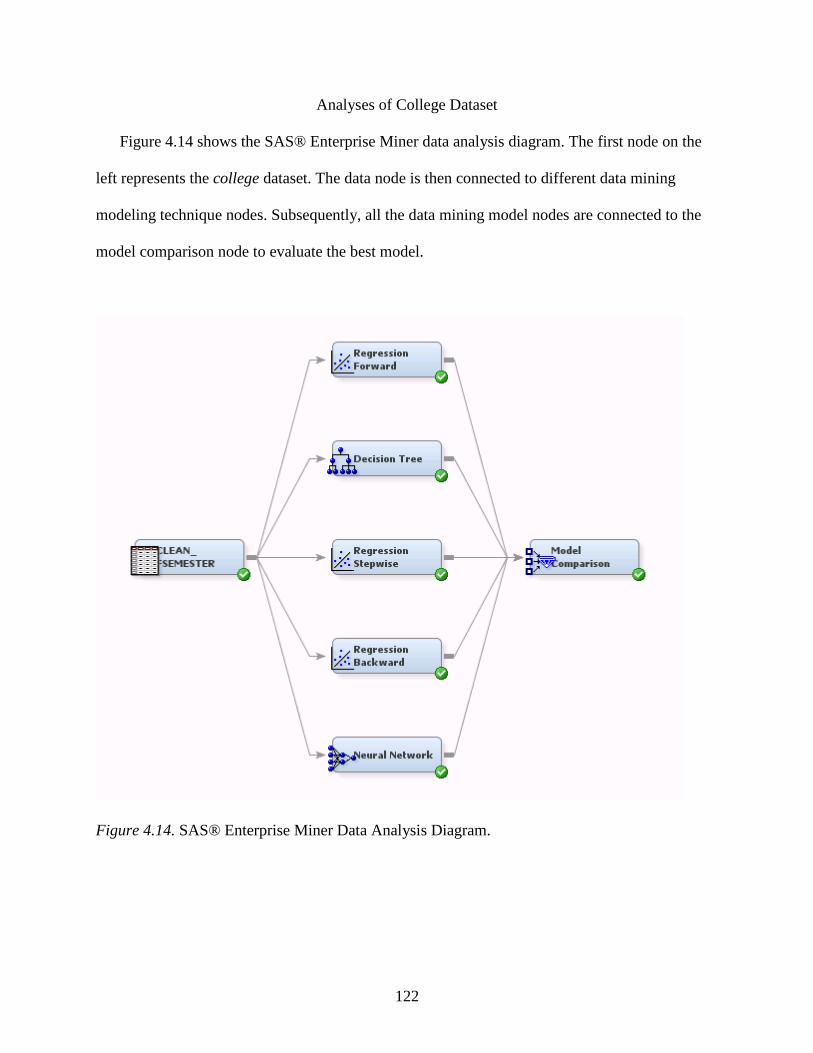
122
Analyses of College Dataset
Figure 4.14 shows the SAS® Enterprise Miner data analysis diagram. The first node on the
left represents the college dataset. The data node is then connected to different data mining
modeling technique nodes. Subsequently, all the data mining model nodes are connected to the
model comparison node to evaluate the best model.
Figure 4.14. SAS® Enterprise Miner Data Analysis Diagram.

123
Forward Regression Results
Figure 4.15. Enterprise Miner Forward Regression Options.
Figure 4.15 shows the forward regression model options. Main effects, two-factor
interactions, and polynomial terms up to second degree order for variables were included in the
model. The model selection criterion was based on valid misclassification rates and the selection
defaults for the model selection technique.
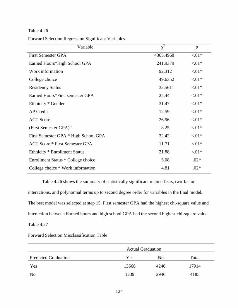
124
Table 4.26
Forward Selection Regression Significant Variables
Variable χ2 p
First Semester GPA 4365.4968 <.01*
Earned Hours*High School GPA 241.9379 <.01*
Work information 92.312 <.01*
College choice 49.6352 <.01*
Residency Status 32.5611 <.01*
Earned Hours*First semester GPA 25.44 <.01*
Ethnicity * Gender 31.47 <.01*
AP Credit 12.59 <.01*
ACT Score 26.96 <.01*
(First Semester GPA) 2 8.25 <.01*
First Semester GPA * High School GPA 32.42 <.01*
ACT Score * First Semester GPA 11.71 <.01*
Ethnicity * Enrollment Status 21.88 <.01*
Enrollment Status * College choice 5.08 .02*
College choice * Work information 4.81 .02*
Table 4.26 shows the summary of statistically significant main effects, two-factor
interactions, and polynomial terms up to second degree order for variables in the final model.
The best model was selected at step 15. First semester GPA had the highest chi-square value and
interaction between Earned hours and high school GPA had the second highest chi-square value.
Table 4.27
Forward Selection Misclassification Table
Actual Graduation
Predicted Graduation Yes No Total
Yes 13668 4246 17914
No 1239 2946 4185

125
Table 4.27 shows a confusion matrix/misclassification table with predicted graduation as
the row variable and actual graduation as the column variable. The misclassification rate was
calculated to evaluate the overall model performance with respect to the exact number of
categorization in the entire data. The diagonal numbers indicate the accurate classifications and
the off diagonal elements indicate the inaccurate classifications (Matignon, 2005). The
misclassification rate for forward selection logistic regression was 24.82%
((1239+4246)/(17914+4185)).
Backward Regression Results
Figure 4.16. Enterprise Miner Backward Regression Options.
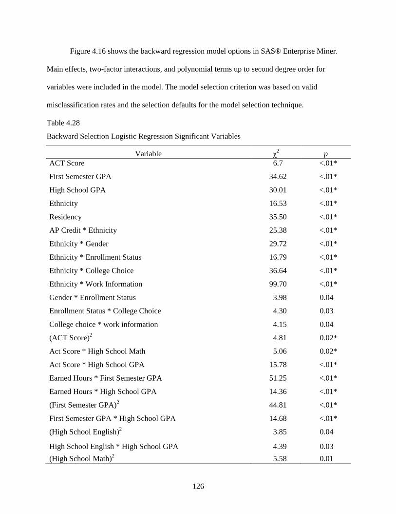
126
Figure 4.16 shows the backward regression model options in SAS® Enterprise Miner.
Main effects, two-factor interactions, and polynomial terms up to second degree order for
variables were included in the model. The model selection criterion was based on valid
misclassification rates and the selection defaults for the model selection technique.
Table 4.28
Backward Selection Logistic Regression Significant Variables
Variable χ2 p
ACT Score 6.7 <.01*
First Semester GPA 34.62 <.01*
High School GPA 30.01 <.01*
Ethnicity 16.53 <.01*
Residency 35.50 <.01*
AP Credit * Ethnicity 25.38 <.01*
Ethnicity * Gender 29.72 <.01*
Ethnicity * Enrollment Status 16.79 <.01*
Ethnicity * College Choice 36.64 <.01*
Ethnicity * Work Information 99.70 <.01*
Gender * Enrollment Status 3.98 0.04
Enrollment Status * College Choice 4.30 0.03
College choice * work information 4.15 0.04
(ACT Score)2 4.81 0.02*
Act Score * High School Math 5.06 0.02*
Act Score * High School GPA 15.78 <.01*
Earned Hours * First Semester GPA 51.25 <.01*
Earned Hours * High School GPA 14.36 <.01*
(First Semester GPA)2 44.81 <.01*
First Semester GPA * High School GPA 14.68 <.01*
(High School English)2 3.85 0.04
High School English * High School GPA 4.39 0.03
(High School Math)2 5.58 0.01
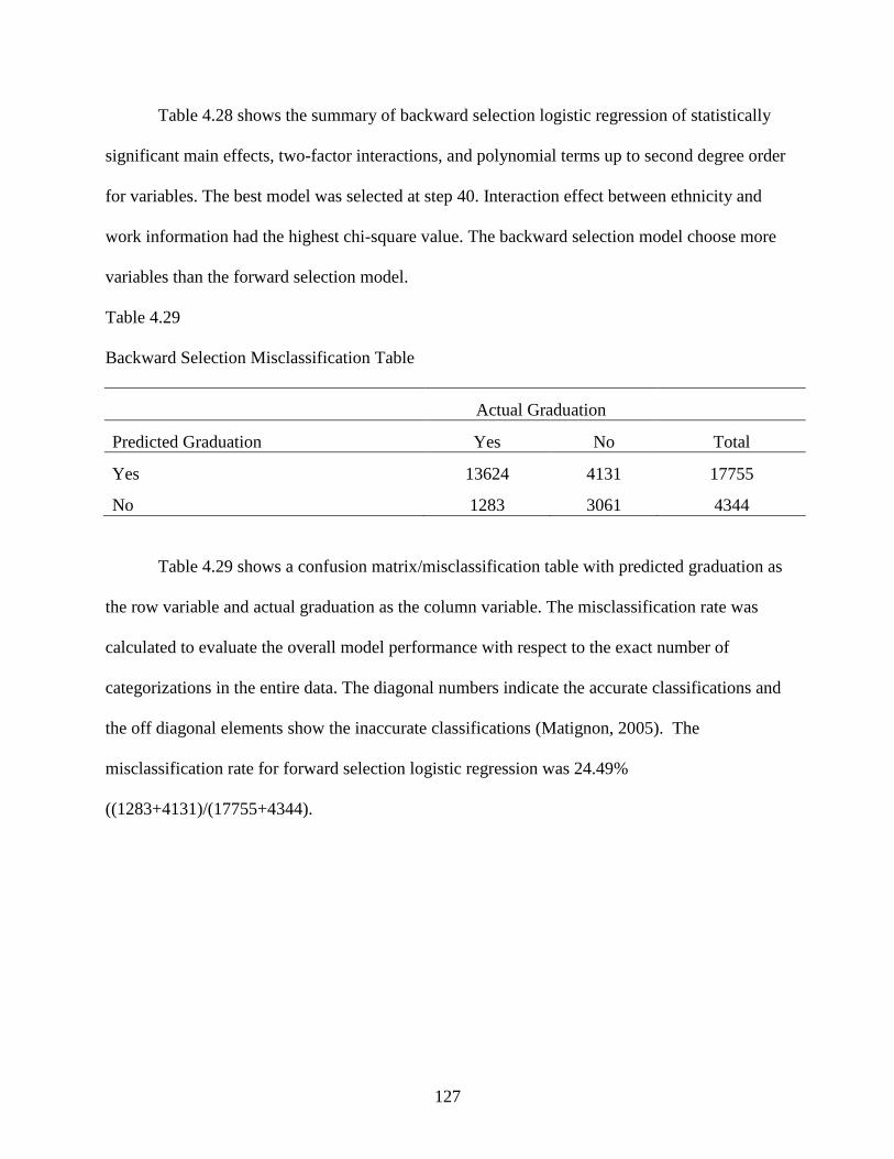
127
Table 4.28 shows the summary of backward selection logistic regression of statistically
significant main effects, two-factor interactions, and polynomial terms up to second degree order
for variables. The best model was selected at step 40. Interaction effect between ethnicity and
work information had the highest chi-square value. The backward selection model choose more
variables than the forward selection model.
Table 4.29
Backward Selection Misclassification Table
Actual Graduation
Predicted Graduation Yes No Total
Yes 13624 4131 17755
No 1283 3061 4344
Table 4.29 shows a confusion matrix/misclassification table with predicted graduation as
the row variable and actual graduation as the column variable. The misclassification rate was
calculated to evaluate the overall model performance with respect to the exact number of
categorizations in the entire data. The diagonal numbers indicate the accurate classifications and
the off diagonal elements show the inaccurate classifications (Matignon, 2005). The
misclassification rate for forward selection logistic regression was 24.49%
((1283+4131)/(17755+4344).
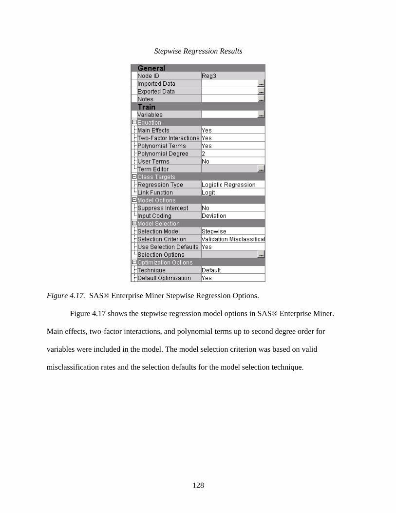
128
Stepwise Regression Results
Figure 4.17. SAS® Enterprise Miner Stepwise Regression Options.
Figure 4.17 shows the stepwise regression model options in SAS® Enterprise Miner.
Main effects, two-factor interactions, and polynomial terms up to second degree order for
variables were included in the model. The model selection criterion was based on valid
misclassification rates and the selection defaults for the model selection technique.
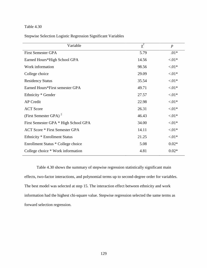
129
Table 4.30
Stepwise Selection Logistic Regression Significant Variables
Variable χ2 p
First Semester GPA 5.79 .01*
Earned Hours*High School GPA 14.56 <.01*
Work information 98.56 <.01*
College choice 29.09 <.01*
Residency Status 35.54 <.01*
Earned Hours*First semester GPA 49.71 <.01*
Ethnicity * Gender 27.57 <.01*
AP Credit 22.98 <.01*
ACT Score 26.31 <.01*
(First Semester GPA) 2 46.43 <.01*
First Semester GPA * High School GPA 34.00 <.01*
ACT Score * First Semester GPA 14.11 <.01*
Ethnicity * Enrollment Status 21.25 <.01*
Enrollment Status * College choice 5.08 0.02*
College choice * Work information 4.81 0.02*
Table 4.30 shows the summary of stepwise regression statistically significant main
effects, two-factor interactions, and polynomial terms up to second-degree order for variables.
The best model was selected at step 15. The interaction effect between ethnicity and work
information had the highest chi-square value. Stepwise regression selected the same terms as
forward selection regression.
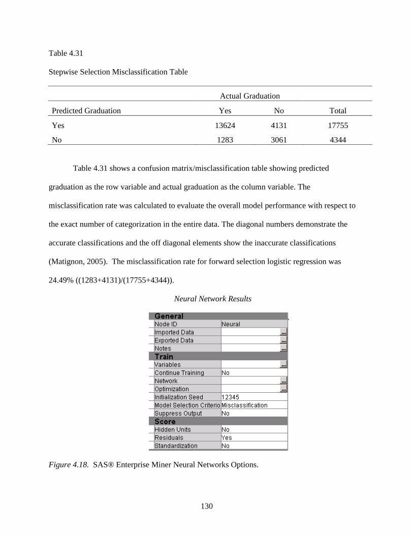
130
Table 4.31
Stepwise Selection Misclassification Table
Actual Graduation
Predicted Graduation Yes No Total
Yes 13624 4131 17755
No 1283 3061 4344
Table 4.31 shows a confusion matrix/misclassification table showing predicted
graduation as the row variable and actual graduation as the column variable. The
misclassification rate was calculated to evaluate the overall model performance with respect to
the exact number of categorization in the entire data. The diagonal numbers demonstrate the
accurate classifications and the off diagonal elements show the inaccurate classifications
(Matignon, 2005). The misclassification rate for forward selection logistic regression was
24.49% ((1283+4131)/(17755+4344)).
Neural Network Results
Figure 4.18. SAS® Enterprise Miner Neural Networks Options.
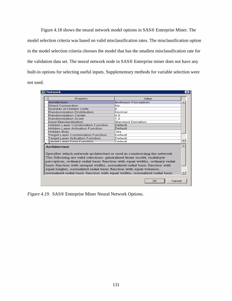
131
Figure 4.18 shows the neural network model options in SAS® Enterprise Miner. The
model selection criteria was based on valid misclassification rates. The misclassification option
in the model selection criteria chooses the model that has the smallest misclassification rate for
the validation data set. The neural network node in SAS® Enterprise miner does not have any
built-in options for selecting useful inputs. Supplementary methods for variable selection were
not used.
Figure 4.19. SAS® Enterprise Miner Neural Network Options.
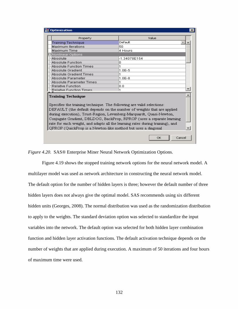
132
Figure 4.20. SAS® Enterprise Miner Neural Network Optimization Options.
Figure 4.19 shows the stopped training network options for the neural network model. A
multilayer model was used as network architecture in constructing the neural network model.
The default option for the number of hidden layers is three; however the default number of three
hidden layers does not always give the optimal model. SAS recommends using six different
hidden units (Georges, 2008). The normal distribution was used as the randomization distribution
to apply to the weights. The standard deviation option was selected to standardize the input
variables into the network. The default option was selected for both hidden layer combination
function and hidden layer activation functions. The default activation technique depends on the
number of weights that are applied during execution. A maximum of 50 iterations and four hours
of maximum time were used.
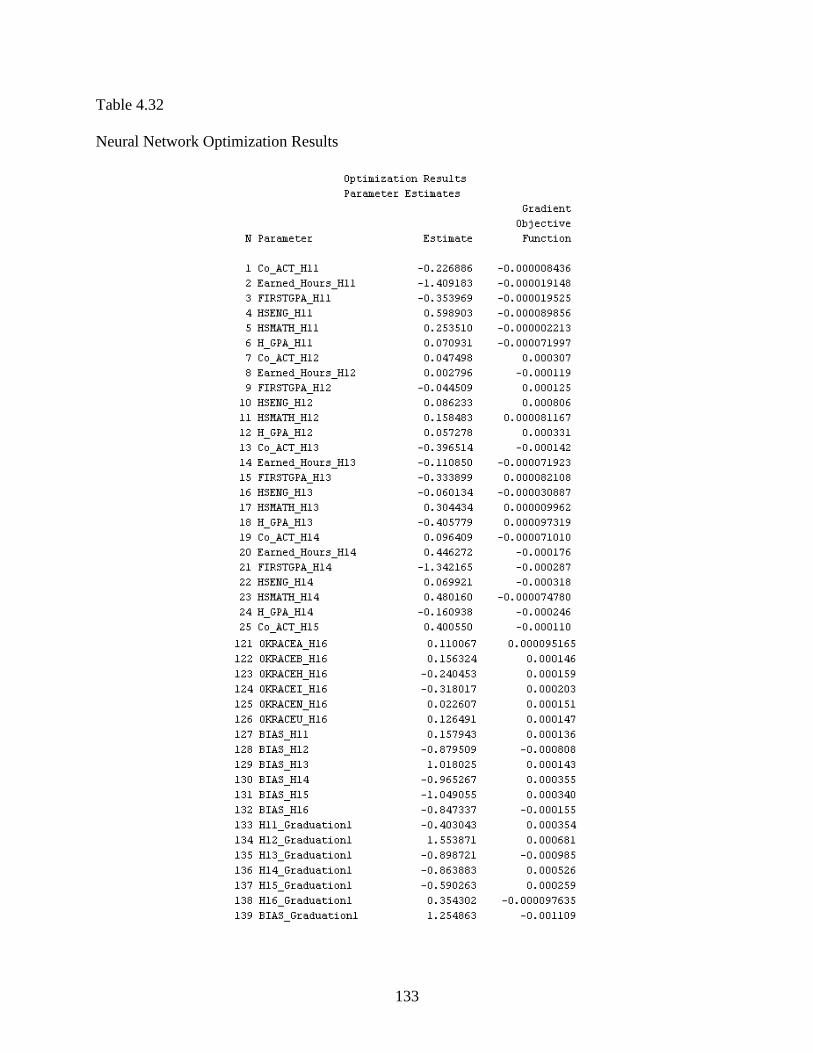
133
Table 4.32
Neural Network Optimization Results
134
Table 4.32 summarizes the neural network model weights. There were 139 parameter
estimates and the overall value of the objective function was 0.51. The generated neural network
model lacked explicability.
Table 4.33
Neural Network Model Misclassification Table
Actual Graduation
Predicted Graduation Yes No Total
Yes 13641 4101 17742
No 1266 3091 4357
Table 4.33 shows a confusion matrix/misclassification table with predicted graduation as
the row variable and actual graduation as the column variable. The misclassification rate was
calculated to evaluate the overall model performance with respect to the exact number of
categorizations in the entire data. The diagonal numbers indicate the accurate classifications and
the off diagonal elements show the inaccurate classifications (Matignon, 2005). The
misclassification rate for neural network model was 24.28% ((1266+4101)/(17742+4357)).
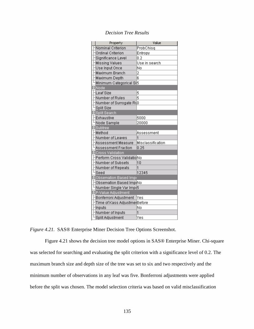
135
Decision Tree Results
Figure 4.21. SAS® Enterprise Miner Decision Tree Options Screenshot.
Figure 4.21 shows the decision tree model options in SAS® Enterprise Miner. Chi-square
was selected for searching and evaluating the split criterion with a significance level of 0.2. The
maximum branch size and depth size of the tree was set to six and two respectively and the
minimum number of observations in any leaf was five. Bonferroni adjustments were applied
before the split was chosen. The model selection criteria was based on valid misclassification
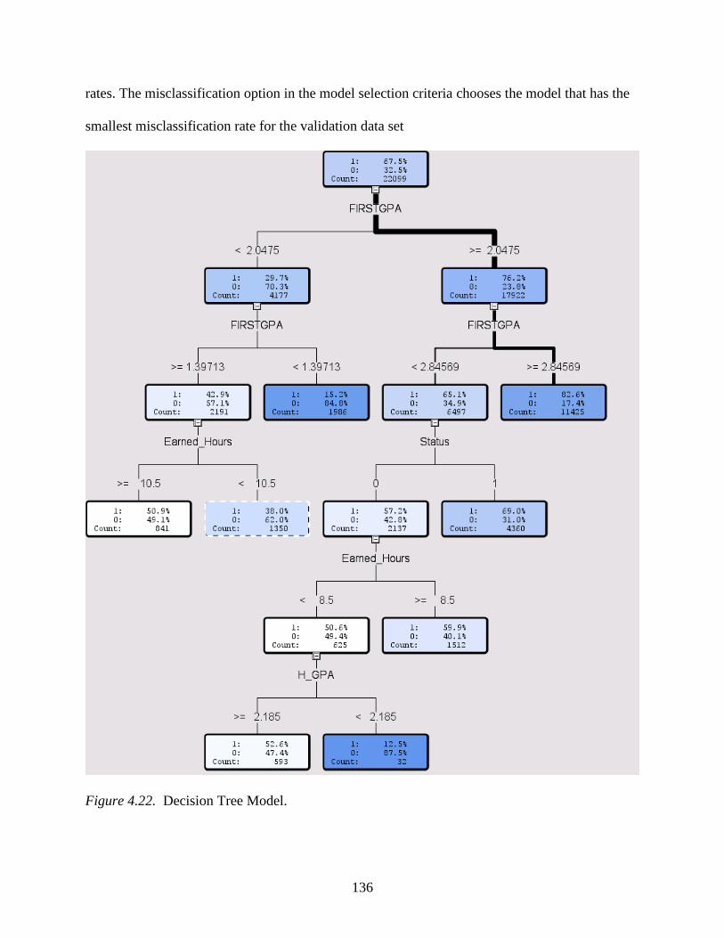
136
rates. The misclassification option in the model selection criteria chooses the model that has the
smallest misclassification rate for the validation data set
Figure 4.22. Decision Tree Model.
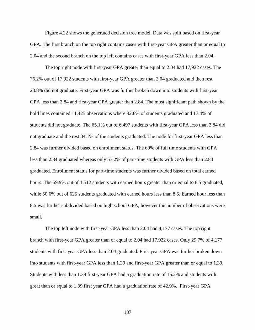
137
Figure 4.22 shows the generated decision tree model. Data was split based on first-year
GPA. The first branch on the top right contains cases with first-year GPA greater than or equal to
2.04 and the second branch on the top left contains cases with first-year GPA less than 2.04.
The top right node with first-year GPA greater than equal to 2.04 had 17,922 cases. The
76.2% out of 17,922 students with first-year GPA greater than 2.04 graduated and then rest
23.8% did not graduate. First-year GPA was further broken down into students with first-year
GPA less than 2.84 and first-year GPA greater than 2.84. The most significant path shown by the
bold lines contained 11,425 observations where 82.6% of students graduated and 17.4% of
students did not graduate. The 65.1% out of 6,497 students with first-year GPA less than 2.84 did
not graduate and the rest 34.1% of the students graduated. The node for first-year GPA less than
2.84 was further divided based on enrollment status. The 69% of full time students with GPA
less than 2.84 graduated whereas only 57.2% of part-time students with GPA less than 2.84
graduated. Enrollment status for part-time students was further divided based on total earned
hours. The 59.9% out of 1,512 students with earned hours greater than or equal to 8.5 graduated,
while 50.6% out of 625 students graduated with earned hours less than 8.5. Earned hour less than
8.5 was further subdivided based on high school GPA, however the number of observations were
small.
The top left node with first-year GPA less than 2.04 had 4,177 cases. The top right
branch with first-year GPA greater than or equal to 2.04 had 17,922 cases. Only 29.7% of 4,177
students with first-year GPA less than 2.04 graduated. First-year GPA was further broken down
into students with first-year GPA less than 1.39 and first-year GPA greater than or equal to 1.39.
Students with less than 1.39 first-year GPA had a graduation rate of 15.2% and students with
great than or equal to 1.39 first year GPA had a graduation rate of 42.9%. First-year GPA
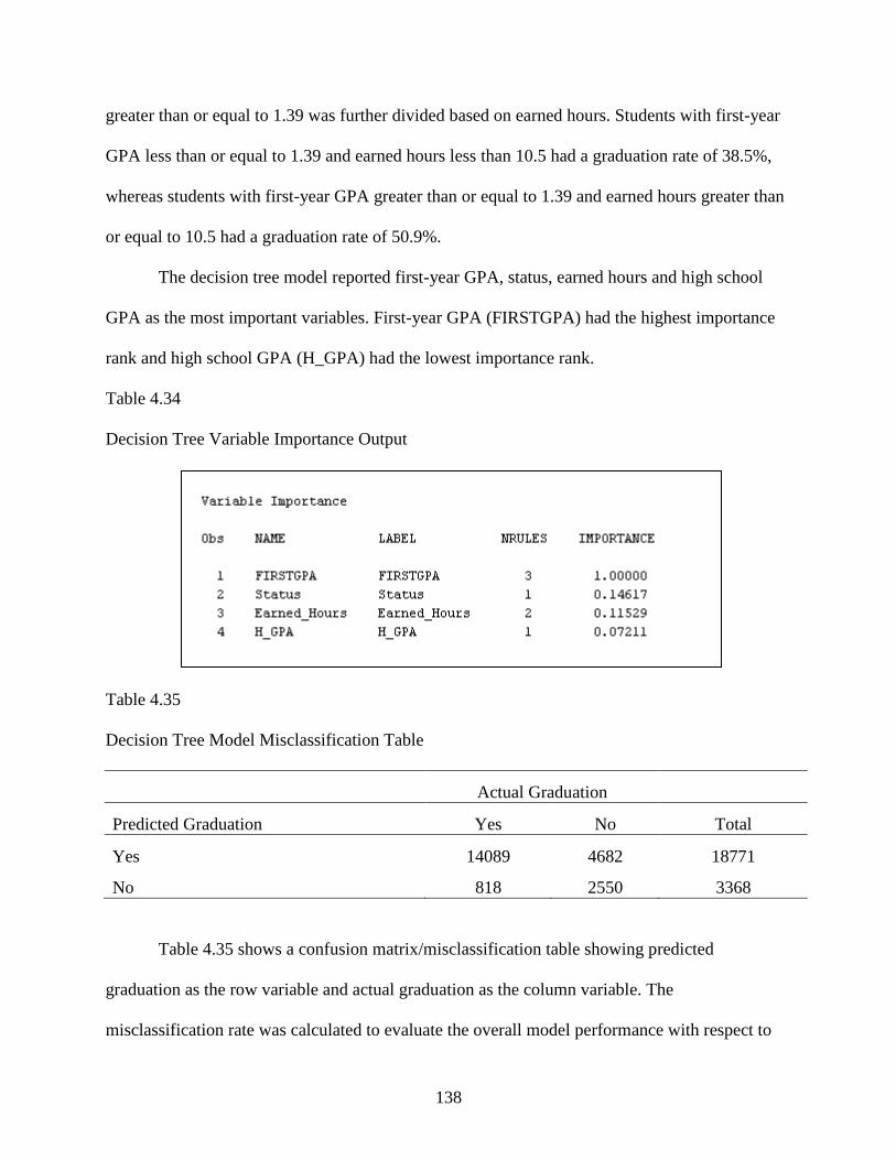
138
greater than or equal to 1.39 was further divided based on earned hours. Students with first-year
GPA less than or equal to 1.39 and earned hours less than 10.5 had a graduation rate of 38.5%,
whereas students with first-year GPA greater than or equal to 1.39 and earned hours greater than
or equal to 10.5 had a graduation rate of 50.9%.
The decision tree model reported first-year GPA, status, earned hours and high school
GPA as the most important variables. First-year GPA (FIRSTGPA) had the highest importance
rank and high school GPA (H_GPA) had the lowest importance rank.
Table 4.34
Decision Tree Variable Importance Output
Table 4.35
Decision Tree Model Misclassification Table
Actual Graduation
Predicted Graduation Yes No Total
Yes 14089 4682 18771
No 818 2550 3368
Table 4.35 shows a confusion matrix/misclassification table showing predicted
graduation as the row variable and actual graduation as the column variable. The
misclassification rate was calculated to evaluate the overall model performance with respect to
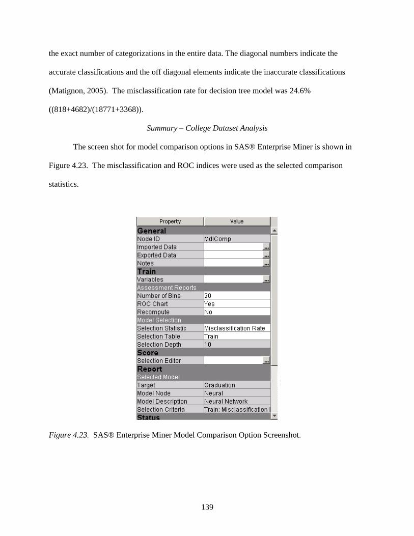
139
the exact number of categorizations in the entire data. The diagonal numbers indicate the
accurate classifications and the off diagonal elements indicate the inaccurate classifications
(Matignon, 2005). The misclassification rate for decision tree model was 24.6%
((818+4682)/(18771+3368)).
Summary – College Dataset Analysis
The screen shot for model comparison options in SAS® Enterprise Miner is shown in
Figure 4.23. The misclassification and ROC indices were used as the selected comparison
statistics.
Figure 4.23. SAS® Enterprise Miner Model Comparison Option Screenshot.
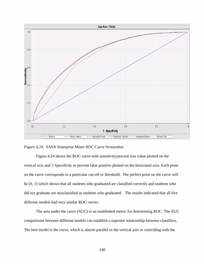
140
Figure 4.24. SAS® Enterprise Miner ROC Curve Screenshot.
Figure 4.24 shows the ROC curve with sensitivity/percent true value plotted on the
vertical axis and 1-Specificity or percent false positive plotted on the horizontal axis. Each point
on the curve corresponds to a particular cut-off or threshold. The perfect point on the curve will
be [0, 1] which shows that all students who graduated are classified correctly and students who
did not graduate are misclassified as students who graduated. The results indicated that all five
different models had very similar ROC curves.
The area under the curve (AUC) is an established metric for determining ROC. The AUC
comparisons between different models can establish a supreme relationship between classifiers.
The best model is the curve, which is almost parallel to the vertical axis or coinciding with the
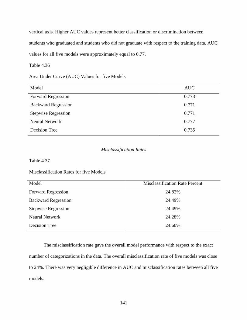
141
vertical axis. Higher AUC values represent better classification or discrimination between
students who graduated and students who did not graduate with respect to the training data. AUC
values for all five models were approximately equal to 0.77.
Table 4.36
Area Under Curve (AUC) Values for five Models
Model AUC
Forward Regression 0.773
Backward Regression 0.771
Stepwise Regression 0.771
Neural Network 0.777
Decision Tree 0.735
Misclassification Rates
Table 4.37
Misclassification Rates for five Models
Model Misclassification Rate Percent
Forward Regression 24.82%
Backward Regression 24.49%
Stepwise Regression 24.49%
Neural Network 24.28%
Decision Tree 24.60%
The misclassification rate gave the overall model performance with respect to the exact
number of categorizations in the data. The overall misclassification rate of five models was close
to 24%. There was very negligible difference in AUC and misclassification rates between all five
models.

142
Research Question Two
The second research question compared different data mining models applied to the pre-
college and college datasets. A 10 fold cross-validation technique was used to build prediction
models for both the pre-college and college datasets. The Statistical software R was used to
build and compare the following models:
1. decision tree;
2. random forests;
3. neural network; and
4. all possible subset regression.
Each of the above data mining models was compared using misclassification rates to find
the best modeling technique. Different R Packages facilitated in building the data mining
models. SAS® Enterprise Miner software does not have the capability to run an n-fold cross-
validation technique and also lacks the ability to build a Random Forests model. Although the
latest SAS® JMP Pro has the capability to run n-fold cross validation, it lacks the ability to run
cross validation for a logistic regression model with a binary target variable. Comparing R to
other SAS products, R is the only package currently that has the capability to run a n-fold cross-
validation and a Random Forests model.
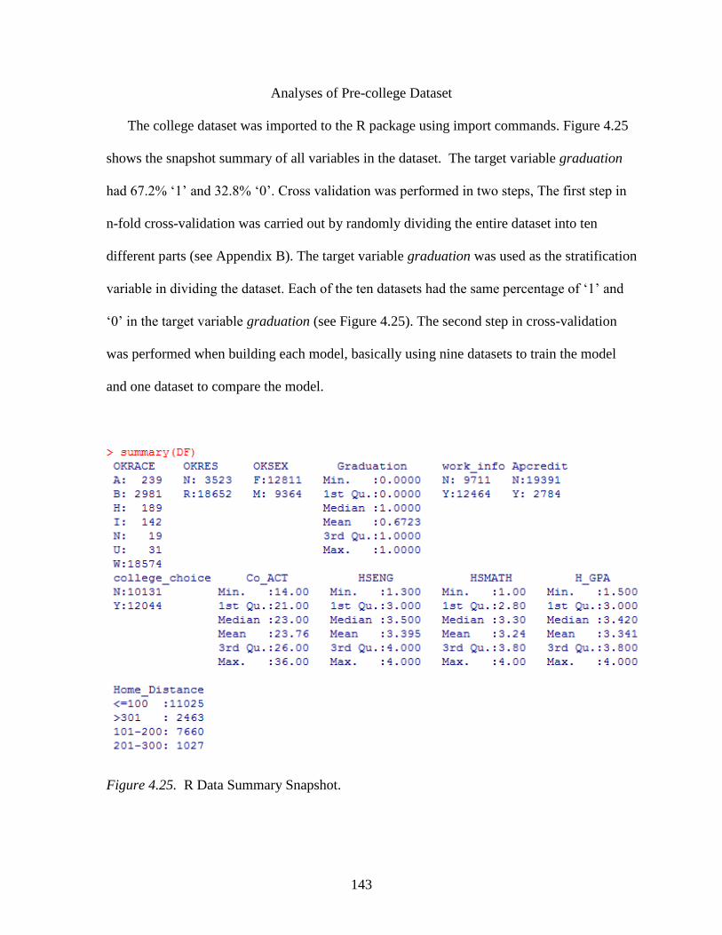
143
Analyses of Pre-college Dataset
The college dataset was imported to the R package using import commands. Figure 4.25
shows the snapshot summary of all variables in the dataset. The target variable graduation
had 67.2% ‘1’ and 32.8% ‘0’. Cross validation was performed in two steps, The first step in
n-fold cross-validation was carried out by randomly dividing the entire dataset into ten
different parts (see Appendix B). The target variable graduation was used as the stratification
variable in dividing the dataset. Each of the ten datasets had the same percentage of ‘1’ and
‘0’ in the target variable graduation (see Figure 4.25). The second step in cross-validation
was performed when building each model, basically using nine datasets to train the model
and one dataset to compare the model.
Figure 4.25. R Data Summary Snapshot.
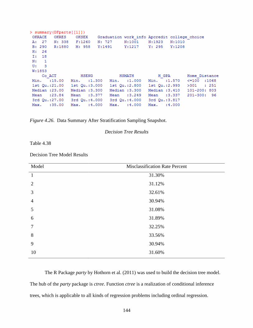
144
Figure 4.26. Data Summary After Stratification Sampling Snapshot.
Decision Tree Results
Table 4.38
Decision Tree Model Results
Model Misclassification Rate Percent
1 31.30%
2 31.12%
3 32.61%
4 30.94%
5 31.08%
6 31.89%
7 32.25%
8 33.56%
9 30.94%
10 31.60%
The R Package party by Hothorn et al. (2011) was used to build the decision tree model.
The hub of the party package is ctree. Function ctree is a realization of conditional inference
trees, which is applicable to all kinds of regression problems including ordinal regression.

145
Function ctree builds decision trees based on recursive partitioning (Hothorn, Hornik, Strobl, &
Zeileis, 2011). The second step in cross-validation was performed by using nine datasets to train
the model and one dataset to compare the model (see Appendix B). The same approach was
repeated ten times so that each dataset was used for comparison. Cross-validation was completed
by calculating the overall misclassification rate using the weighted average of all ten
misclassification rates. Table 4.38 shows the misclassification rates for each model. The average
overall misclassification rate was 31.7%.
Neural Network Results
Table 4.39
Neural Network Model Results
Model Misclassification Rate
1 31.74%
2 30.88%
3 33.31%
4 30.83%
5 32.77%
6 30.92%
7 32.32%
8 33.27%
9 30.74%
10 31.17%
The R Package nnet was used to build the neural network model. Function nnet builds
single hidden layer neural networks (Ripley, 2009). The second step in cross-validation was
performed by using nine datasets to train the model and one dataset to compare the model
resulting in ten misclassification rates (see Appendix B). The same approach was repeated ten
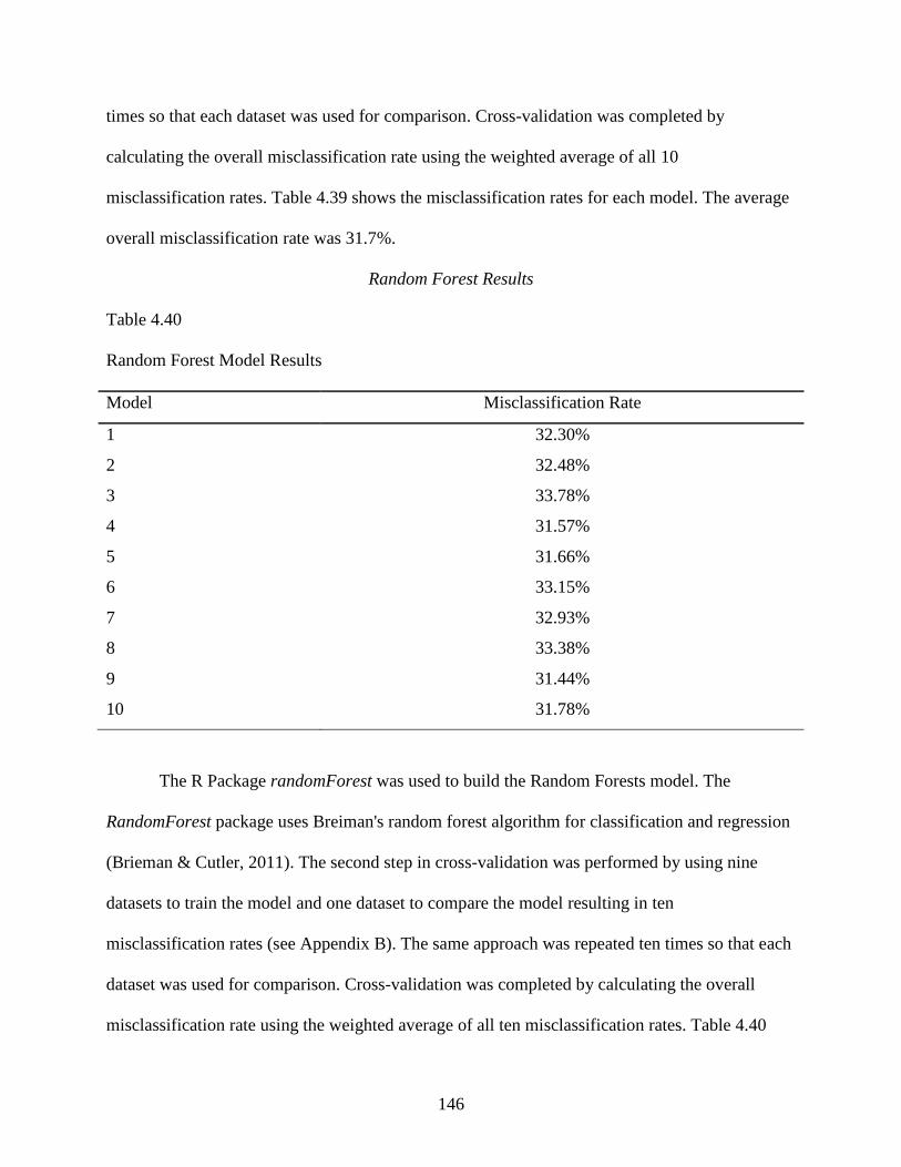
146
times so that each dataset was used for comparison. Cross-validation was completed by
calculating the overall misclassification rate using the weighted average of all 10
misclassification rates. Table 4.39 shows the misclassification rates for each model. The average
overall misclassification rate was 31.7%.
Random Forest Results
Table 4.40
Random Forest Model Results
Model Misclassification Rate
1 32.30%
2 32.48%
3 33.78%
4 31.57%
5 31.66%
6 33.15%
7 32.93%
8 33.38%
9 31.44%
10 31.78%
The R Package randomForest was used to build the Random Forests model. The
RandomForest package uses Breiman's random forest algorithm for classification and regression
(Brieman & Cutler, 2011). The second step in cross-validation was performed by using nine
datasets to train the model and one dataset to compare the model resulting in ten
misclassification rates (see Appendix B). The same approach was repeated ten times so that each
dataset was used for comparison. Cross-validation was completed by calculating the overall
misclassification rate using the weighted average of all ten misclassification rates. Table 4.40
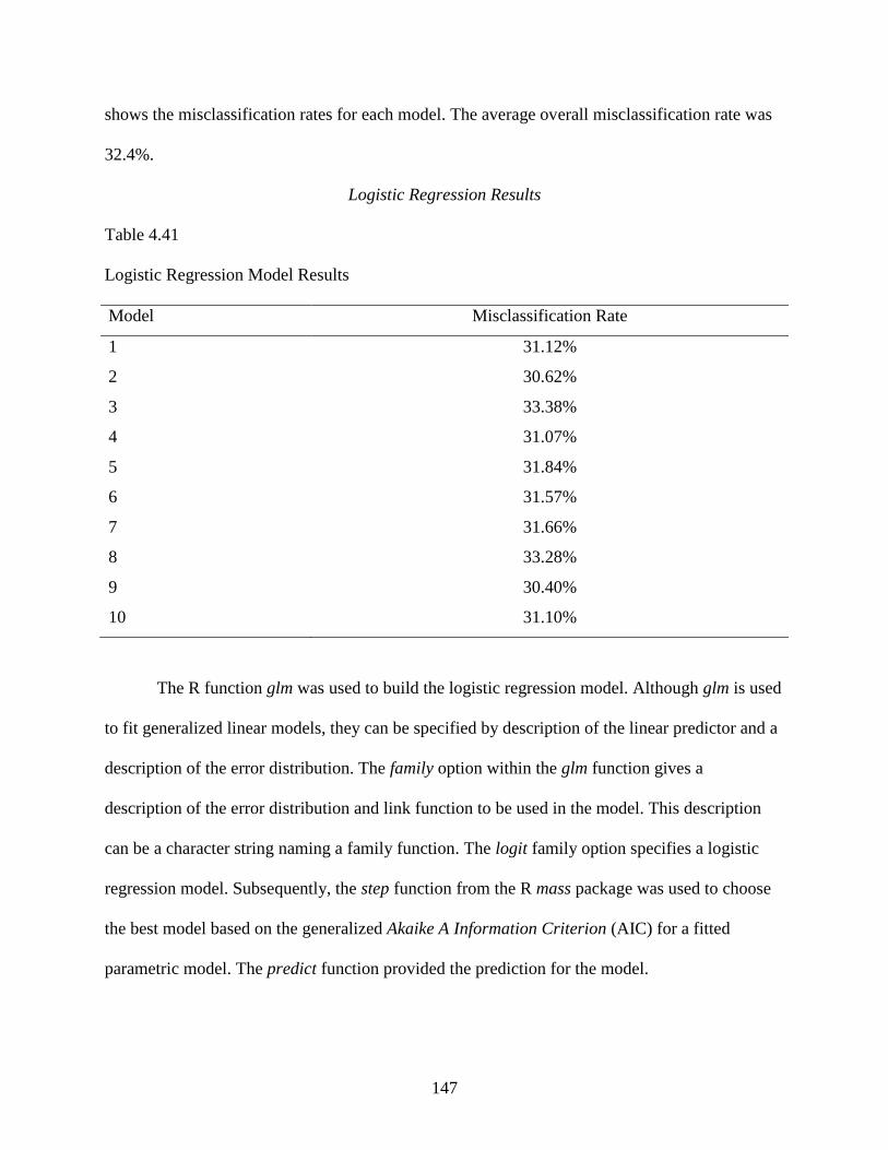
147
shows the misclassification rates for each model. The average overall misclassification rate was
32.4%.
Logistic Regression Results
Table 4.41
Logistic Regression Model Results
Model Misclassification Rate
1 31.12%
2 30.62%
3 33.38%
4 31.07%
5 31.84%
6 31.57%
7 31.66%
8 33.28%
9 30.40%
10 31.10%
The R function glm was used to build the logistic regression model. Although glm is used
to fit generalized linear models, they can be specified by description of the linear predictor and a
description of the error distribution. The family option within the glm function gives a
description of the error distribution and link function to be used in the model. This description
can be a character string naming a family function. The logit family option specifies a logistic
regression model. Subsequently, the step function from the R mass package was used to choose
the best model based on the generalized Akaike A Information Criterion (AIC) for a fitted
parametric model. The predict function provided the prediction for the model.
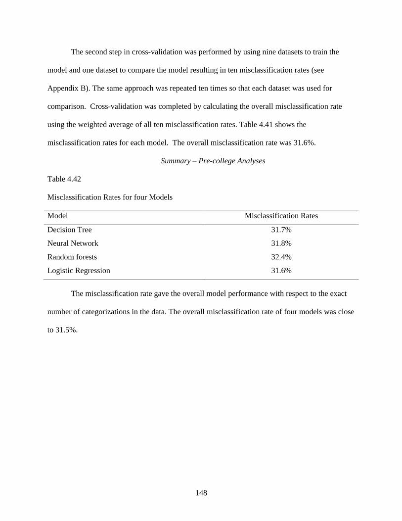
148
The second step in cross-validation was performed by using nine datasets to train the
model and one dataset to compare the model resulting in ten misclassification rates (see
Appendix B). The same approach was repeated ten times so that each dataset was used for
comparison. Cross-validation was completed by calculating the overall misclassification rate
using the weighted average of all ten misclassification rates. Table 4.41 shows the
misclassification rates for each model. The overall misclassification rate was 31.6%.
Summary – Pre-college Analyses
Table 4.42
Misclassification Rates for four Models
Model Misclassification Rates
Decision Tree 31.7%
Neural Network 31.8%
Random forests 32.4%
Logistic Regression 31.6%
The misclassification rate gave the overall model performance with respect to the exact
number of categorizations in the data. The overall misclassification rate of four models was close
to 31.5%.

149
Analyses of College Dataset
The college dataset was input in the R package using import commands. Figure 4.25
shows the snapshot summary of all variables in the dataset. The target variable graduation had
67.2% ‘1’ and 32.8% ‘0’. Cross validation was performed in two steps. The first step in n-fold
cross-validation was carried out by randomly dividing the entire dataset into ten different parts
(see Appendix B). The target variable graduation was used as the stratification variable in
dividing the dataset. Each of the ten datasets had the same percentage of ‘1’ and ‘0’ in the target
variable graduation (see Figure 4.25). The second step in cross-validation was performed when
building each model, basically using nine datasets to train the model and one dataset to compare
the model.
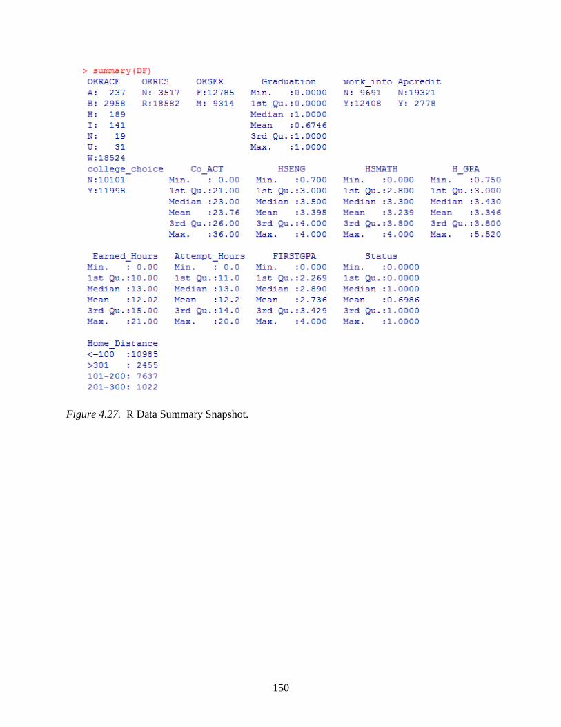
150
Figure 4.27. R Data Summary Snapshot.
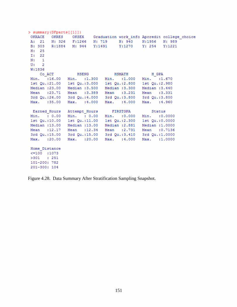
151
Figure 4.28. Data Summary After Stratification Sampling Snapshot.
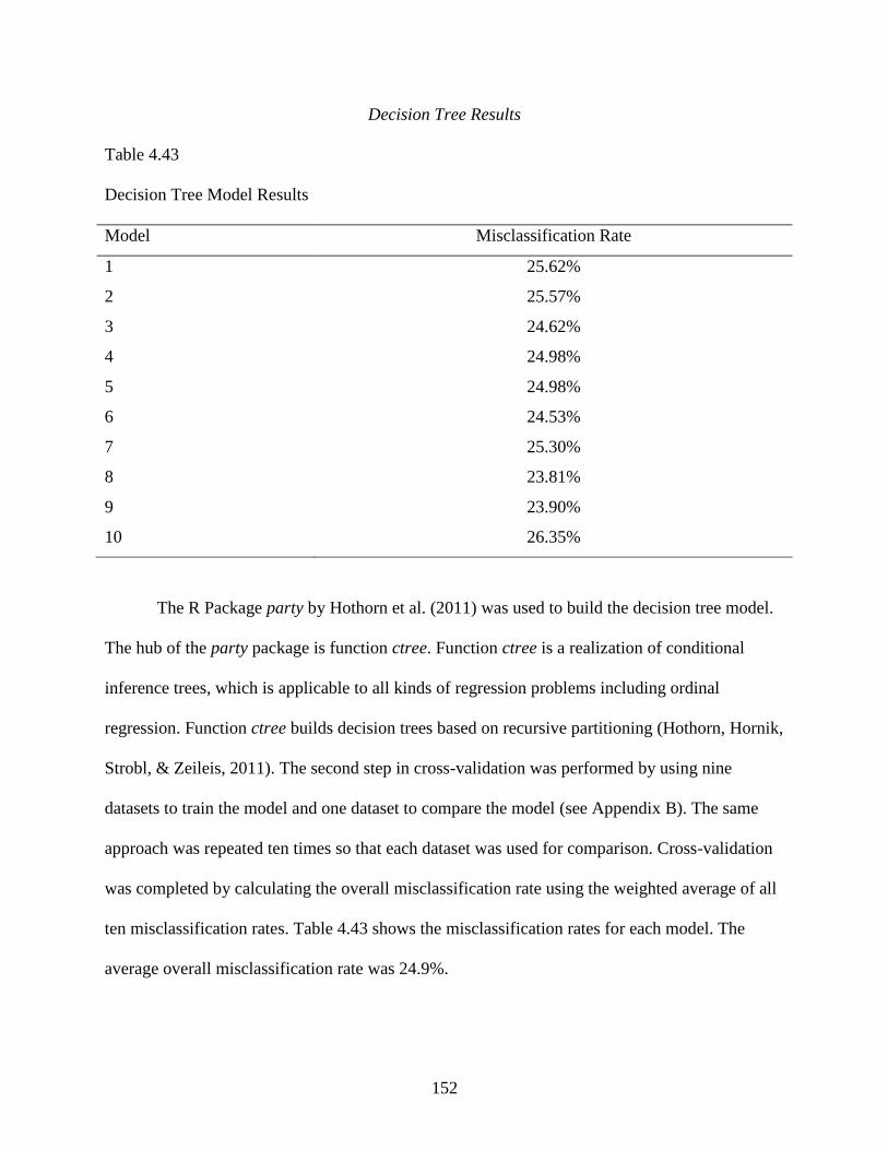
152
Decision Tree Results
Table 4.43
Decision Tree Model Results
Model Misclassification Rate
1 25.62%
2 25.57%
3 24.62%
4 24.98%
5 24.98%
6 24.53%
7 25.30%
8 23.81%
9 23.90%
10 26.35%
The R Package party by Hothorn et al. (2011) was used to build the decision tree model.
The hub of the party package is function ctree. Function ctree is a realization of conditional
inference trees, which is applicable to all kinds of regression problems including ordinal
regression. Function ctree builds decision trees based on recursive partitioning (Hothorn, Hornik,
Strobl, & Zeileis, 2011). The second step in cross-validation was performed by using nine
datasets to train the model and one dataset to compare the model (see Appendix B). The same
approach was repeated ten times so that each dataset was used for comparison. Cross-validation
was completed by calculating the overall misclassification rate using the weighted average of all
ten misclassification rates. Table 4.43 shows the misclassification rates for each model. The
average overall misclassification rate was 24.9%.

153
Neural Network Results
Table 4.44
Neural Network Model Results
Model Misclassification Rate Percent
1 32.53%
2 24.66%
3 25.00%
4 24.93%
5 24.20%
6 25.02%
7 24.16%
8 32.53%
9 25.80%
10 32.53%
The R Package nnet was used to build the neural network model. Function nnet builds
single hidden layer neural networks (Ripley, 2009). The Second step in cross-validation was
performed by using nine datasets to train the model and one dataset to compare the model
resulting in ten misclassification rates (see Appendix B). The same approach was repeated ten
times so that each dataset was used for comparison. Cross-validation was completed by
calculating the overall misclassification rate using the weighted average of all ten
misclassification rates. Table 4.44 shows the misclassification rates for each model. The average
overall misclassification rate was 27.1%.
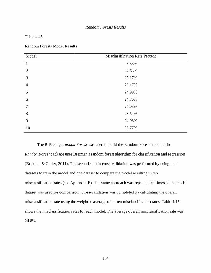
154
Random Forests Results
Table 4.45
Random Forests Model Results
Model Misclassification Rate Percent
1 25.53%
2 24.63%
3 25.17%
4 25.17%
5 24.99%
6 24.76%
7 25.08%
8 23.54%
9 24.08%
10 25.77%
The R Package randomForest was used to build the Random Forests model. The
RandomForest package uses Breiman's random forest algorithm for classification and regression
(Brieman & Cutler, 2011). The second step in cross-validation was performed by using nine
datasets to train the model and one dataset to compare the model resulting in ten
misclassification rates (see Appendix B). The same approach was repeated ten times so that each
dataset was used for comparison. Cross-validation was completed by calculating the overall
misclassification rate using the weighted average of all ten misclassification rates. Table 4.45
shows the misclassification rates for each model. The average overall misclassification rate was
24.8%.
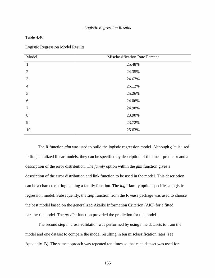
155
Logistic Regression Results
Table 4.46
Logistic Regression Model Results
Model Misclassification Rate Percent
1 25.48%
2 24.35%
3 24.67%
4 26.12%
5 25.26%
6 24.06%
7 24.98%
8 23.90%
9 23.72%
10 25.63%
The R function glm was used to build the logistic regression model. Although glm is used
to fit generalized linear models, they can be specified by description of the linear predictor and a
description of the error distribution. The family option within the glm function gives a
description of the error distribution and link function to be used in the model. This description
can be a character string naming a family function. The logit family option specifies a logistic
regression model. Subsequently, the step function from the R mass package was used to choose
the best model based on the generalized Akaike Information Criterion (AIC) for a fitted
parametric model. The predict function provided the prediction for the model.
The second step in cross-validation was performed by using nine datasets to train the
model and one dataset to compare the model resulting in ten misclassification rates (see
Appendix B). The same approach was repeated ten times so that each dataset was used for
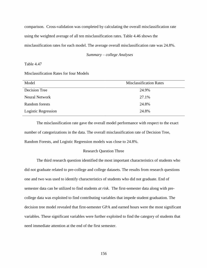
156
comparison. Cross-validation was completed by calculating the overall misclassification rate
using the weighted average of all ten misclassification rates. Table 4.46 shows the
misclassification rates for each model. The average overall misclassification rate was 24.8%.
Summary – college Analyses
Table 4.47
Misclassification Rates for four Models
Model Misclassification Rates
Decision Tree 24.9%
Neural Network 27.1%
Random forests 24.8%
Logistic Regression 24.8%
The misclassification rate gave the overall model performance with respect to the exact
number of categorizations in the data. The overall misclassification rate of Decision Tree,
Random Forests, and Logistic Regression models was close to 24.8%.
Research Question Three
The third research question identified the most important characteristics of students who
did not graduate related to pre-college and college datasets. The results from research questions
one and two was used to identify characteristics of students who did not graduate. End of
semester data can be utilized to find students at risk. The first-semester data along with pre-
college data was exploited to find contributing variables that impede student graduation. The
decision tree model revealed that first-semester GPA and earned hours were the most significant
variables. These significant variables were further exploited to find the category of students that
need immediate attention at the end of the first semester.
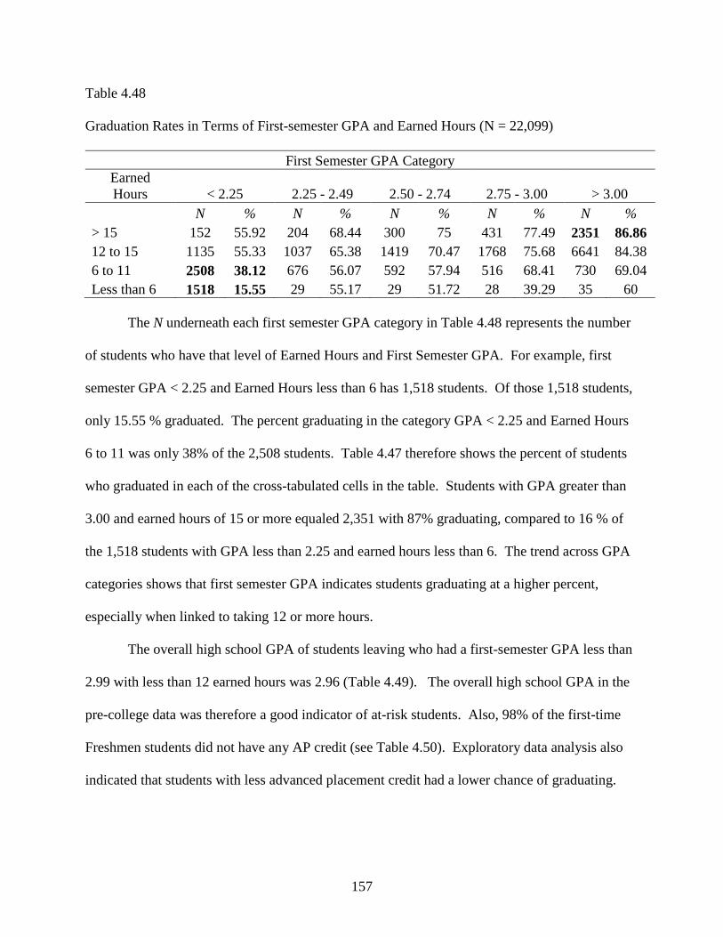
157
Table 4.48
Graduation Rates in Terms of First-semester GPA and Earned Hours (N = 22,099)
First Semester GPA Category
Earned
Hours < 2.25 2.25 - 2.49 2.50 - 2.74 2.75 - 3.00 > 3.00
N % N % N % N % N %
> 15 152 55.92 204 68.44 300 75 431 77.49 2351 86.86
12 to 15 1135 55.33 1037 65.38 1419 70.47 1768 75.68 6641 84.38
6 to 11 2508 38.12 676 56.07 592 57.94 516 68.41 730 69.04
Less than 6 1518 15.55 29 55.17 29 51.72 28 39.29 35 60
The N underneath each first semester GPA category in Table 4.48 represents the number
of students who have that level of Earned Hours and First Semester GPA. For example, first
semester GPA < 2.25 and Earned Hours less than 6 has 1,518 students. Of those 1,518 students,
only 15.55 % graduated. The percent graduating in the category GPA < 2.25 and Earned Hours
6 to 11 was only 38% of the 2,508 students. Table 4.47 therefore shows the percent of students
who graduated in each of the cross-tabulated cells in the table. Students with GPA greater than
3.00 and earned hours of 15 or more equaled 2,351 with 87% graduating, compared to 16 % of
the 1,518 students with GPA less than 2.25 and earned hours less than 6. The trend across GPA
categories shows that first semester GPA indicates students graduating at a higher percent,
especially when linked to taking 12 or more hours.
The overall high school GPA of students leaving who had a first-semester GPA less than
2.99 with less than 12 earned hours was 2.96 (Table 4.49). The overall high school GPA in the
pre-college data was therefore a good indicator of at-risk students. Also, 98% of the first-time
Freshmen students did not have any AP credit (see Table 4.50). Exploratory data analysis also
indicated that students with less advanced placement credit had a lower chance of graduating.
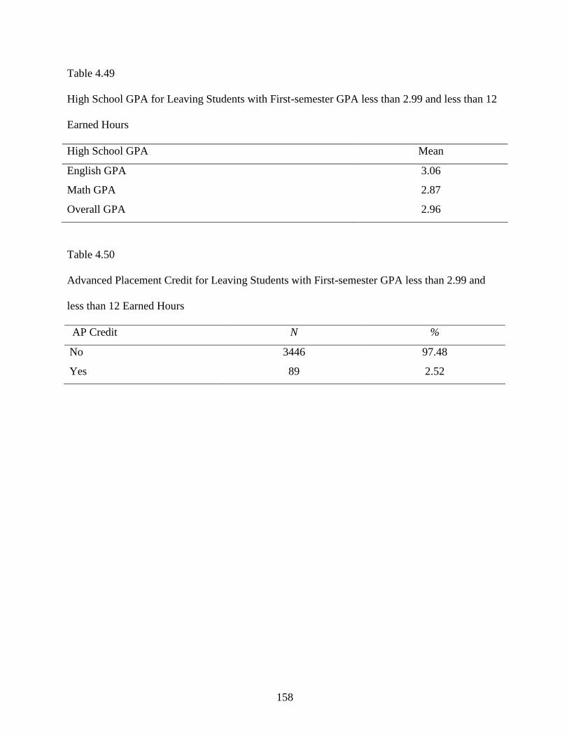
158
Table 4.49
High School GPA for Leaving Students with First-semester GPA less than 2.99 and less than 12
Earned Hours
High School GPA Mean
English GPA 3.06
Math GPA 2.87
Overall GPA 2.96
Table 4.50
Advanced Placement Credit for Leaving Students with First-semester GPA less than 2.99 and
less than 12 Earned Hours
AP Credit N %
No 3446 97.48
Yes 89 2.52

159
CHAPTER V:
SUMMARY, CONCLUSIONS, AND RECOMMENDATIONS
Introduction
Research studies have focused on single sets of variables, which only explain a small
percentage of variation in graduation. Higher education research desires more sophisticated
models that can take into account multiple variables that relate to student graduation. In addition,
there are major gaps in higher education literature with respect to research on overall graduation.
Most studies concentrate on retention beyond the first-year in college and not on graduation.
To address these concerns, this research study compared data mining techniques on key
variables leading to student graduation at The University of Alabama. This research study
compared the statistical predictive data mining models of logistic regression with four different
variable selection methods, decision tree, random forests and neural networks using SAS and R
statistical software. The statistical models facilitated finding the most important characteristics of
first-time Freshmen students who graduate. This chapter results from the data mining techniques,
a comparison of model performance results, along with recommendations for building data
mining models on institutional data. Recommendations are made based on the identification of
student characteristics that improve student graduation.
The study used available data at The University of Alabama to predict six-year
graduation rates and discover the most important student characteristics that lead to graduation
for incoming Freshmen both at the beginning and the end of the first semester. Extensive work
was done to acquire, clean, prepare and analyze the data used for the analysis and statistical
160
modeling. Data preparation was facilitated using SAS® and SAS® JMP, while data analysis was
done using SAS® Enterprise Miner and R programs. Missing data was assumed to be missing at
random; therefore a list-wise deletion method was adopted to clean the missing data.
Mahalanobis distance assisted in making decisions about deleting outliers. Two datasets, pre-
college and college were created with graduation as the target variable. The pre-college dataset
contained demographics, high school, and ACT information, whereas, the college dataset
contained variables in the pre-college dataset as well as end of semester college information.
Summary of Findings
Exploratory Data Analysis
Following data preparation, statistical exploratory were used to inspect the student data
set using graphical charts and descriptive statistics. Every variable in both datasets were explored
in terms of the graduation target variable. The graduation rate for Freshmen students enrolled
from 1995 to 2005 at The University of Alabama increased from 1,750 students in 1995 to 2,389
students in 2005. The overall increase in Freshmen student enrollment in the span of ten years
accounts for 36.5%. Even though enrollment rates had increased, the average overall graduation
rate for incoming Freshmen students has remained around 67.46%.
Demographic Variables
Female student enrollment from 1995 – 2005 constituted about 58% and 42% male
enrollment. The overall graduation rate for first-time Freshmen females was 70.49% compared to
63.29% for males. Caucasian and African American students shared the majority of the
Freshmen enrollment with 83% and 13.3% respectively. Caucasian students graduated at a 7%
higher than African American students.
161
The overall resident student enrollment constituted about 84% compared to 16% for non-
resident students. Resident students had an overall graduation rate of around 68% and non-
resident students had an overall graduation rate of 64%. Freshmen students with home distance
between 0 - 200 miles had an overall graduation rate of around 68%, whereas Freshmen students
with home distance greater than 200 miles had a graduation rate of 64%.
High School Variables
Freshmen students who had advanced placement credit were approximately 10%
compared to 90% of Freshmen students with no advanced placement credits. The overall
graduation rate for students with advanced placement credit was approximately 84% and
graduation rate for students with no advanced placement credit was around 65%. Overall high
school English GPA, Math GPA, and average GPA for graduated students was 3.48, 3.33, and
3.44 respectively. English GPA, Math GPA, and overall GPA for leaving students were 3.23,
3.05, and 3.15, respectively.
ACT Variables
Freshmen students choosing Alabama to be their first choice on ACT profile information
constituted around 54% compared to 46% of Freshmen students who chose universities other
universities. First-choice students had an overall graduation rate that was 3% higher than
students who chose other universities. Freshmen students who chose to work on ACT profile
information constitute around 56% compared to 44% of Freshmen students who chose not to
work. Students who expected not to work during college on ACT profile information had an
overall graduation rate of that was 7% higher than students who expected to work during college.
The overall average ACT score for students who graduated was 24.2, whereas the average ACT
score for students who did not graduate was 22.84.

162
College Variables
The total overall full-time students constituted around 70% compared to 30% for part-
time students. The overall graduation rate for full-time students was around 78% and students
with part-time status had an overall graduation rate of around 42%. Therefore, full-time students
(greater than 12 earned credit hours) had significantly higher graduation rates of around 36%
more than part-time students (less than 12 earned credit hours). The average first-semester GPA
for students who graduated was 3.03, whereas average first-semester GPA for leaving students
was 2.13. Finally, the average first-semester earned hours for students who graduated was around
13 hours and for leavers it was less than ten hours.
Research Question One
The first research question analyzed the most important characteristics related to pre-
college and college datasets. SAS Enterprise Miner analyzed logistic regression (forward,
backward, stepwise), neural networks, and decision tree data mining methodologies to compare
the best model using misclassification and receiver operation characteristics curve.
Pre-college dataset
Logistic regression with forward variable selection method indicated a high chi-square
value for work information and advanced placement credit with an overall misclassification rate
of 31.23%. Logistic regression with backward selection method showed interaction between
ethnicity and advanced placement credit and also included more interaction terms in the model
than the forward selection method; however, the data indicated very similar misclassification
rates. Stepwise regression specified the same terms in the model as the forward selection method
with misclassification rate of 30.86%. Neural network model indicated a misclassification rate
close to 31%, but due to lack of explicability, important variables in the model could not be
163
interpreted. The decision tree model indicated high school GPA, work information, ethnicity,
college choice, and residency as the most important variables, respectively, with a
misclassification rate close to 31%. All data mining models had similar ROC indices.
College dataset
Logistic regression with forward variable selection method indicated a high chi-square
value for first semester GPA, and interaction between earned hours and high school GPA with an
overall misclassification rate of 24.82%. Logistic regression with backward selection method
included more terms in the model, but indicated very similar misclassification rates. Stepwise
regression specified the same terms in the model as forward selection method with a
misclassification rate of 24.49%. Neural network model indicated a misclassification rate of
24.28%, but due to lack of explicability important variables in the model could not be
interpreted. The decision tree model indicated first semester GPA, status, earned hours, and high
school GPA as the most important variables, respectively, and had a misclassification rate of
24.6%. Finally, all data mining models had similar misclassification rates and ROC indices.
Research Question Two
The second research question compared different data mining modes related to the pre-
college and college datasets. The R statistical program using a 10 fold cross-validation
technique analyzed logistic regression with stepwise variable selection, neural networks, decision
tree, and random forests data mining methodologies to determine the best model using
misclassification rates.
Pre-College Dataset
The overall misclassification rate for decision trees, neural network, logistic regression,
and random forests was 31.7%, 31.8%, 32.4%, and 31.6% respectively.
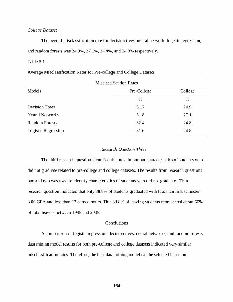
164
College Dataset
The overall misclassification rate for decision trees, neural network, logistic regression,
and random forests was 24.9%, 27.1%, 24.8%, and 24.8% respectively.
Table 5.1
Average Misclassification Rates for Pre-college and College Datasets
Misclassification Rates
Models Pre-College College
% %
Decision Trees 31.7 24.9
Neural Networks 31.8 27.1
Random Forests 32.4 24.8
Logistic Regression 31.6 24.8
Research Question Three
The third research question identified the most important characteristics of students who
did not graduate related to pre-college and college datasets. The results from research questions
one and two was used to identify characteristics of students who did not graduate. Third
research question indicated that only 38.8% of students graduated with less than first semester
3.00 GPA and less than 12 earned hours. This 38.8% of leaving students represented about 50%
of total leavers between 1995 and 2005.
Conclusions
A comparison of logistic regression, decision trees, neural networks, and random forests
data mining model results for both pre-college and college datasets indicated very similar
misclassification rates. Therefore, the best data mining model can be selected based on

165
advantages and disadvantages. Some of the disadvantages when using a logistic regression
model include (Tufféry, 2011) the following:
1. Explanatory variables must be linearly independent, else could lead to collinearity
problems;
2. Cannot handle the missing values of continuous variables; and
3. Sensitive to extreme values of continuous variables.
Student data can contain several variables out of which two or more predictors can be highly
correlated. This Multi-collinearity can lead to unstable estimates, with possibly incoherent
results. Student datasets also have missing data. Although there are several different ways to fix
multicollinearity and impute missing values, these steps can involve more time and resources,
but should be done prior to data mining.
One of the biggest disadvantages of neural network models includes lack of explanatory
power. That is; discovery of important variables in the model. Neural network models are
termed a black box because the hidden layer cannot be usually interpreted because of the
unavailability of the calculated weights (Nisbet, Elder, & Miner, 2009).
Random forests produce complex trees for complex dimensional datasets where the
contribution of a single variable in the classification rule gets lost (Tutz, 2012). Although
decision trees have some disadvantages, the biggest advantage is that they are self explanatory
and easy to follow, which makes it easy for non-statistical professionals (Rokach & Maimo,
2008). Decision trees can also handle missing values; using all the information in the dataset and
saving additional steps and resources compared to logistic regression. Decision trees provide a
better practical interpretation of results compared to logistic regression, neural networks, and
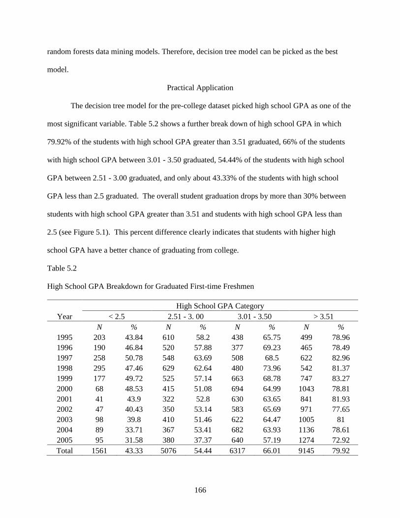
166
random forests data mining models. Therefore, decision tree model can be picked as the best
model.
Practical Application
The decision tree model for the pre-college dataset picked high school GPA as one of the
most significant variable. Table 5.2 shows a further break down of high school GPA in which
79.92% of the students with high school GPA greater than 3.51 graduated, 66% of the students
with high school GPA between 3.01 - 3.50 graduated, 54.44% of the students with high school
GPA between 2.51 - 3.00 graduated, and only about 43.33% of the students with high school
GPA less than 2.5 graduated. The overall student graduation drops by more than 30% between
students with high school GPA greater than 3.51 and students with high school GPA less than
2.5 (see Figure 5.1). This percent difference clearly indicates that students with higher high
school GPA have a better chance of graduating from college.
Table 5.2
High School GPA Breakdown for Graduated First-time Freshmen
High School GPA Category
Year < 2.5 2.51 - 3. 00 3.01 - 3.50 > 3.51
N % N % N % N %
1995 203 43.84 610 58.2 438 65.75 499 78.96
1996 190 46.84 520 57.88 377 69.23 465 78.49
1997 258 50.78 548 63.69 508 68.5 622 82.96
1998 295 47.46 629 62.64 480 73.96 542 81.37
1999 177 49.72 525 57.14 663 68.78 747 83.27
2000 68 48.53 415 51.08 694 64.99 1043 78.81
2001 41 43.9 322 52.8 630 63.65 841 81.93
2002 47 40.43 350 53.14 583 65.69 971 77.65
2003 98 39.8 410 51.46 622 64.47 1005 81
2004 89 33.71 367 53.41 682 63.93 1136 78.61
2005 95 31.58 380 37.37 640 57.19 1274 72.92
Total 1561 43.33 5076 54.44 6317 66.01 9145 79.92
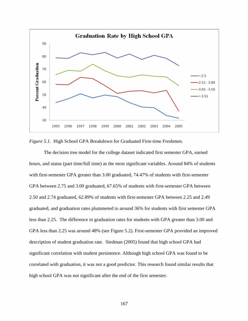
167
Figure 5.1. High School GPA Breakdown for Graduated First-time Freshmen.
The decision tree model for the college dataset indicated first semester GPA, earned
hours, and status (part time/full time) as the most significant variables. Around 84% of students
with first-semester GPA greater than 3.00 graduated, 74.47% of students with first-semester
GPA between 2.75 and 3.00 graduated, 67.65% of students with first-semester GPA between
2.50 and 2.74 graduated, 62.89% of students with first-semester GPA between 2.25 and 2.49
graduated, and graduation rates plummeted to around 36% for students with first semester GPA
less than 2.25. The difference in graduation rates for students with GPA greater than 3.00 and
GPA less than 2.25 was around 48% (see Figure 5.2). First-semester GPA provided an improved
description of student graduation rate. Siedman (2005) found that high school GPA had
significant correlation with student persistence. Although high school GPA was found to be
correlated with graduation, it was not a good predictor. This research found similar results that
high school GPA was not significant after the end of the first semester.
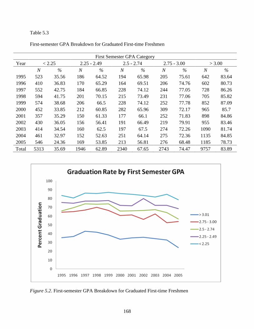
168
Table 5.3
First-semester GPA Breakdown for Graduated First-time Freshmen
First Semester GPA Category
Year < 2.25 2.25 - 2.49 2.5 - 2.74 2.75 - 3.00 > 3.00
N % N % N % N % N %
1995 523 35.56 186 64.52 194 65.98 205 75.61 642 83.64
1996 410 36.83 170 65.29 164 69.51 206 74.76 602 80.73
1997 552 42.75 184 66.85 228 74.12 244 77.05 728 86.26
1998 594 41.75 201 70.15 215 73.49 231 77.06 705 85.82
1999 574 38.68 206 66.5 228 74.12 252 77.78 852 87.09
2000 452 33.85 212 60.85 282 65.96 309 72.17 965 85.7
2001 357 35.29 150 61.33 177 66.1 252 71.83 898 84.86
2002 430 36.05 156 56.41 191 66.49 219 79.91 955 83.46
2003 414 34.54 160 62.5 197 67.5 274 72.26 1090 81.74
2004 461 32.97 152 52.63 251 64.14 275 72.36 1135 84.85
2005 546 24.36 169 53.85 213 56.81 276 68.48 1185 78.73
Total 5313 35.69 1946 62.89 2340 67.65 2743 74.47 9757 83.89
Figure 5.2. First-semester GPA Breakdown for Graduated First-time Freshmen
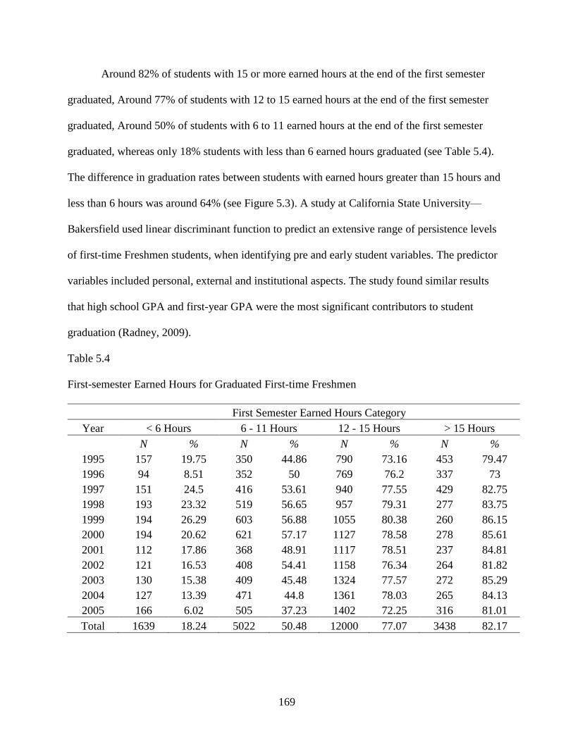
169
Around 82% of students with 15 or more earned hours at the end of the first semester
graduated, Around 77% of students with 12 to 15 earned hours at the end of the first semester
graduated, Around 50% of students with 6 to 11 earned hours at the end of the first semester
graduated, whereas only 18% students with less than 6 earned hours graduated (see Table 5.4).
The difference in graduation rates between students with earned hours greater than 15 hours and
less than 6 hours was around 64% (see Figure 5.3). A study at California State University—
Bakersfield used linear discriminant function to predict an extensive range of persistence levels
of first-time Freshmen students, when identifying pre and early student variables. The predictor
variables included personal, external and institutional aspects. The study found similar results
that high school GPA and first-year GPA were the most significant contributors to student
graduation (Radney, 2009).
Table 5.4
First-semester Earned Hours for Graduated First-time Freshmen
First Semester Earned Hours Category
Year < 6 Hours 6 - 11 Hours 12 - 15 Hours > 15 Hours
N % N % N % N %
1995 157 19.75 350 44.86 790 73.16 453 79.47
1996 94 8.51 352 50 769 76.2 337 73
1997 151 24.5 416 53.61 940 77.55 429 82.75
1998 193 23.32 519 56.65 957 79.31 277 83.75
1999 194 26.29 603 56.88 1055 80.38 260 86.15
2000 194 20.62 621 57.17 1127 78.58 278 85.61
2001 112 17.86 368 48.91 1117 78.51 237 84.81
2002 121 16.53 408 54.41 1158 76.34 264 81.82
2003 130 15.38 409 45.48 1324 77.57 272 85.29
2004 127 13.39 471 44.8 1361 78.03 265 84.13
2005 166 6.02 505 37.23 1402 72.25 316 81.01
Total 1639 18.24 5022 50.48 12000 77.07 3438 82.17
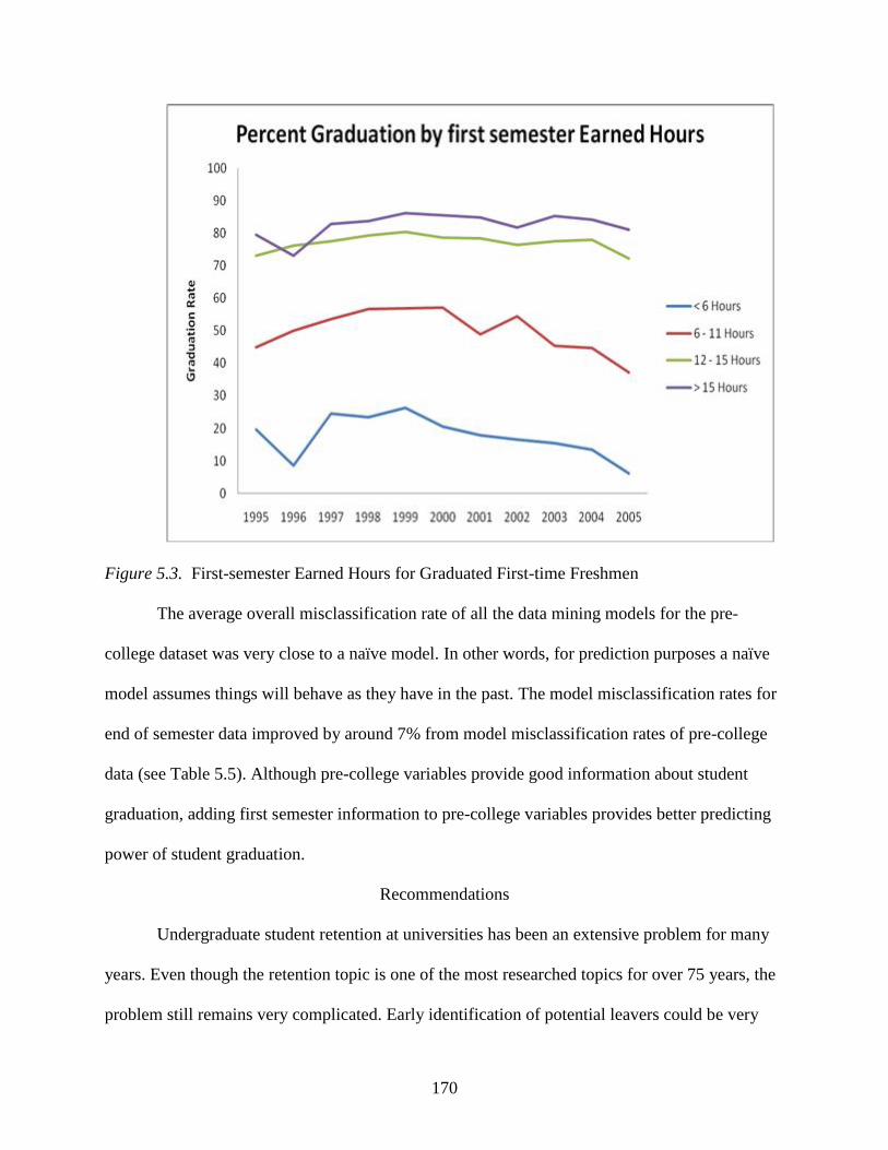
170
Figure 5.3. First-semester Earned Hours for Graduated First-time Freshmen
The average overall misclassification rate of all the data mining models for the pre-
college dataset was very close to a naïve model. In other words, for prediction purposes a naïve
model assumes things will behave as they have in the past. The model misclassification rates for
end of semester data improved by around 7% from model misclassification rates of pre-college
data (see Table 5.5). Although pre-college variables provide good information about student
graduation, adding first semester information to pre-college variables provides better predicting
power of student graduation.
Recommendations
Undergraduate student retention at universities has been an extensive problem for many
years. Even though the retention topic is one of the most researched topics for over 75 years, the
problem still remains very complicated. Early identification of potential leavers could be very
171
beneficial for students and institutions. Research studies indicated that early identification of
leaving students and intervention program are key to understanding what factors lead to student
graduation.
Institutions should utilize Siedman’s retention formula for student success:
RETention = Early (Identification) + (Early + Intensive + Continuous) Intervention.
Early identification of potential leavers and successful intervention program(s) are the key for
improving student graduation.
A research study showed that pre-college grades and perceptions of academic ability
were directly correlated to a decrease in students GPA from high school to college. The research
found that the most compelling indicator of drop in GPA was due to academic disengagement
(Keup, 2009). This study also found similar results in that first semester GPA was a significant
predictor of student graduation. Programs related to academic disengagement should be
developed and implemented for students identified as “at risk” using the decision tree data
mining model.
University of Louisville, for example, offers several programs that assist students in
improving their academic skills and performance in college courses, better prepare students to
adapt to college life, and improve retention rates of first-year lower division undergraduate
students (University of Louisville, 2012). Some of their programs to improve retention include:
mentoring program for first-year students conducted by trained second year students, reach out
programs to increase person to person contact with a discussion of strategies for success, and
student success seminars.
Noel-Levitz (2009) conducted a web-based study concerning student retention practices
to determine most effective retention practices for public and private, two-year and four-year

172
institutions. They concluded that “academic support programs, programs designed to raise the
retention rates of first-year students and placing an institution-wide emphasis on teaching and
learning” (p. 1) were the top best student retention practices.
Institutions can use historical end of first-semester data along with high school
information to build decision tree models that find significant variables contributing to student
graduation. Students at risk can be predicted at the end of the first semester instead of waiting
until the end of the first year of school. The results from data mining analyses can be used to
develop intervention programs to help students succeed in college and graduate.
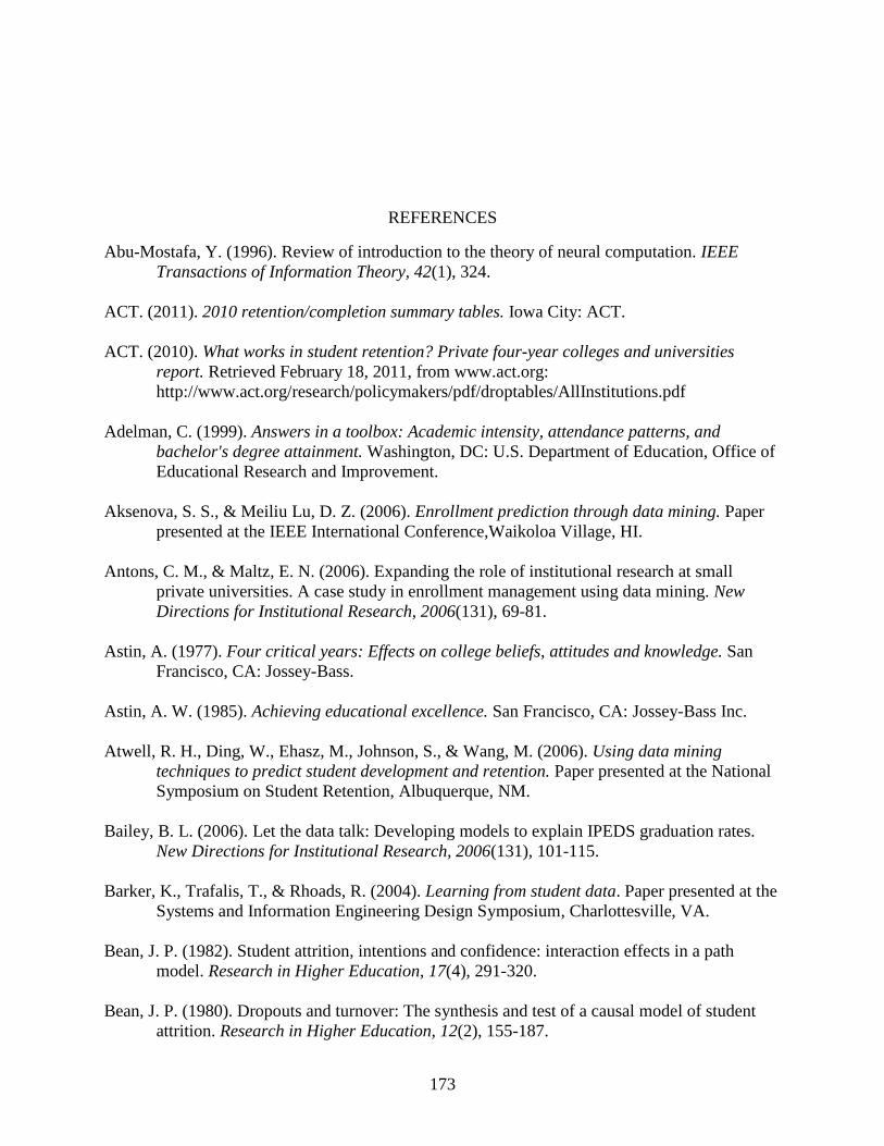
173
REFERENCES
Abu-Mostafa, Y. (1996). Review of introduction to the theory of neural computation. IEEE
Transactions of Information Theory, 42(1), 324.
ACT. (2011). 2010 retention/completion summary tables. Iowa City: ACT.
ACT. (2010). What works in student retention? Private four-year colleges and universities
report. Retrieved February 18, 2011, from www.act.org:
http://www.act.org/research/policymakers/pdf/droptables/AllInstitutions.pdf
Adelman, C. (1999). Answers in a toolbox: Academic intensity, attendance patterns, and
bachelor's degree attainment. Washington, DC: U.S. Department of Education, Office of
Educational Research and Improvement.
Aksenova, S. S., & Meiliu Lu, D. Z. (2006). Enrollment prediction through data mining. Paper
presented at the IEEE International Conference,Waikoloa Village, HI.
Antons, C. M., & Maltz, E. N. (2006). Expanding the role of institutional research at small
private universities. A case study in enrollment management using data mining. New
Directions for Institutional Research, 2006(131), 69-81.
Astin, A. (1977). Four critical years: Effects on college beliefs, attitudes and knowledge. San
Francisco, CA: Jossey-Bass.
Astin, A. W. (1985). Achieving educational excellence. San Francisco, CA: Jossey-Bass Inc.
Atwell, R. H., Ding, W., Ehasz, M., Johnson, S., & Wang, M. (2006). Using data mining
techniques to predict student development and retention. Paper presented at the National
Symposium on Student Retention, Albuquerque, NM.
Bailey, B. L. (2006). Let the data talk: Developing models to explain IPEDS graduation rates.
New Directions for Institutional Research, 2006(131), 101-115.
Barker, K., Trafalis, T., & Rhoads, R. (2004). Learning from student data. Paper presented at the
Systems and Information Engineering Design Symposium, Charlottesville, VA.
Bean, J. P. (1982). Student attrition, intentions and confidence: interaction effects in a path
model. Research in Higher Education, 17(4), 291-320.
Bean, J. P. (1980). Dropouts and turnover: The synthesis and test of a causal model of student
attrition. Research in Higher Education, 12(2), 155-187.
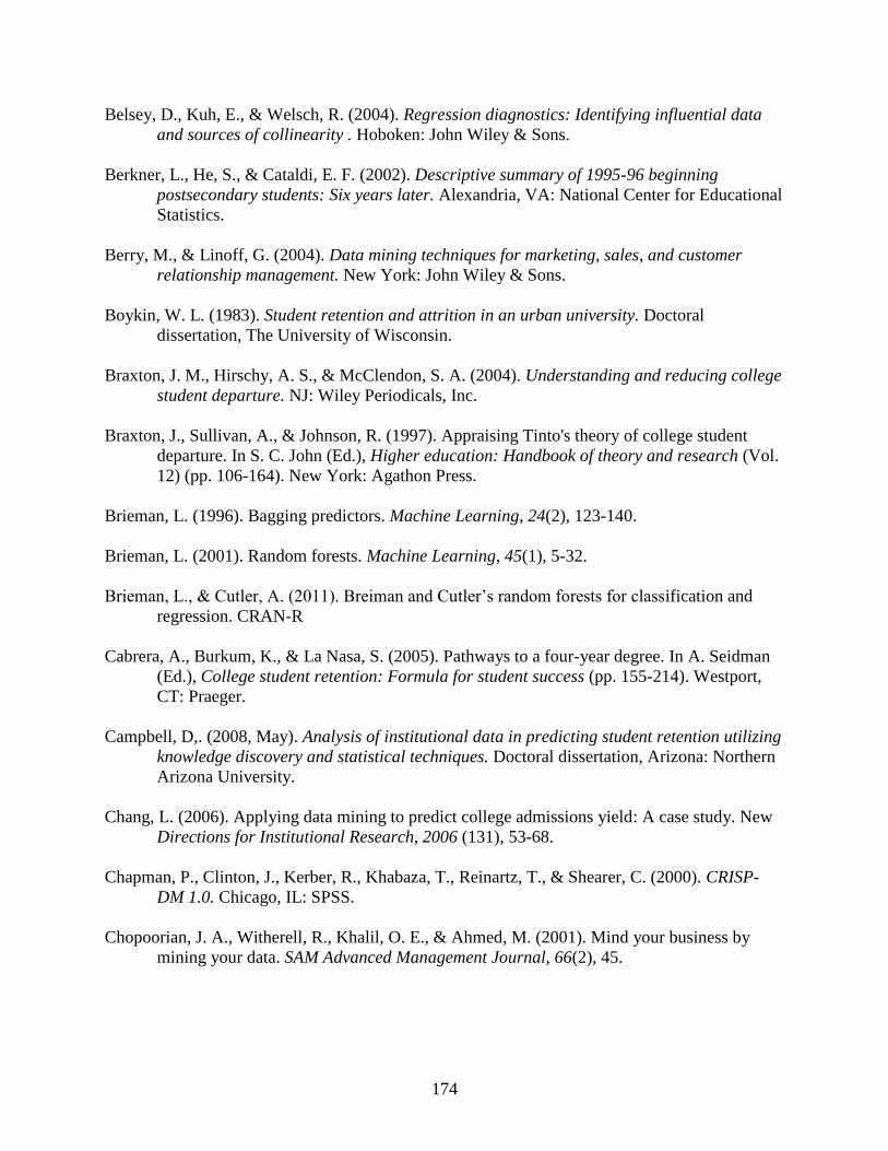
174
Belsey, D., Kuh, E., & Welsch, R. (2004). Regression diagnostics: Identifying influential data
and sources of collinearity . Hoboken: John Wiley & Sons.
Berkner, L., He, S., & Cataldi, E. F. (2002). Descriptive summary of 1995-96 beginning
postsecondary students: Six years later. Alexandria, VA: National Center for Educational
Statistics.
Berry, M., & Linoff, G. (2004). Data mining techniques for marketing, sales, and customer
relationship management. New York: John Wiley & Sons.
Boykin, W. L. (1983). Student retention and attrition in an urban university. Doctoral
dissertation, The University of Wisconsin.
Braxton, J. M., Hirschy, A. S., & McClendon, S. A. (2004). Understanding and reducing college
student departure. NJ: Wiley Periodicals, Inc.
Braxton, J., Sullivan, A., & Johnson, R. (1997). Appraising Tinto's theory of college student
departure. In S. C. John (Ed.), Higher education: Handbook of theory and research (Vol.
12) (pp. 106-164). New York: Agathon Press.
Brieman, L. (1996). Bagging predictors. Machine Learning, 24(2), 123-140.
Brieman, L. (2001). Random forests. Machine Learning, 45(1), 5-32.
Brieman, L., & Cutler, A. (2011). Breiman and Cutler’s random forests for classification and
regression. CRAN-R
Cabrera, A., Burkum, K., & La Nasa, S. (2005). Pathways to a four-year degree. In A. Seidman
(Ed.), College student retention: Formula for student success (pp. 155-214). Westport,
CT: Praeger.
Campbell, D,. (2008, May). Analysis of institutional data in predicting student retention utilizing
knowledge discovery and statistical techniques. Doctoral dissertation, Arizona: Northern
Arizona University.
Chang, L. (2006). Applying data mining to predict college admissions yield: A case study. New
Directions for Institutional Research, 2006 (131), 53-68.
Chapman, P., Clinton, J., Kerber, R., Khabaza, T., Reinartz, T., & Shearer, C. (2000). CRISP-
DM 1.0. Chicago, IL: SPSS.
Chopoorian, J. A., Witherell, R., Khalil, O. E., & Ahmed, M. (2001). Mind your business by
mining your data. SAM Advanced Management Journal, 66(2), 45.
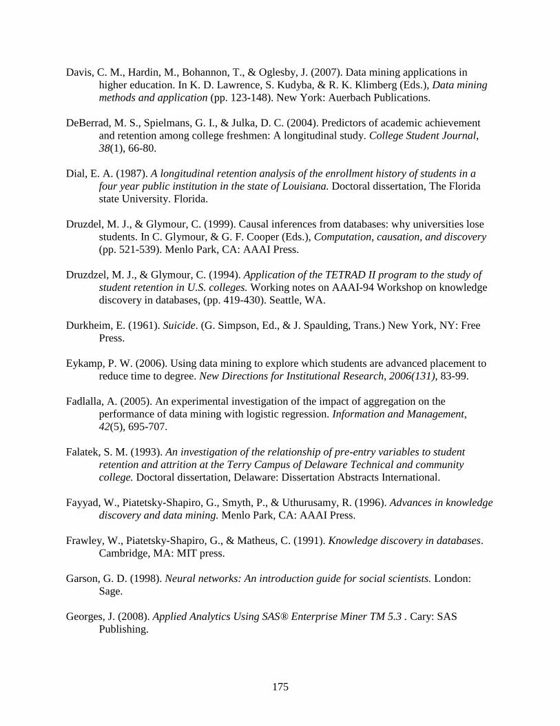
175
Davis, C. M., Hardin, M., Bohannon, T., & Oglesby, J. (2007). Data mining applications in
higher education. In K. D. Lawrence, S. Kudyba, & R. K. Klimberg (Eds.), Data mining
methods and application (pp. 123-148). New York: Auerbach Publications.
DeBerrad, M. S., Spielmans, G. I., & Julka, D. C. (2004). Predictors of academic achievement
and retention among college freshmen: A longitudinal study. College Student Journal,
38(1), 66-80.
Dial, E. A. (1987). A longitudinal retention analysis of the enrollment history of students in a
four year public institution in the state of Louisiana. Doctoral dissertation, The Florida
state University. Florida.
Druzdel, M. J., & Glymour, C. (1999). Causal inferences from databases: why universities lose
students. In C. Glymour, & G. F. Cooper (Eds.), Computation, causation, and discovery
(pp. 521-539). Menlo Park, CA: AAAI Press.
Druzdzel, M. J., & Glymour, C. (1994). Application of the TETRAD II program to the study of
student retention in U.S. colleges. Working notes on AAAI-94 Workshop on knowledge
discovery in databases, (pp. 419-430). Seattle, WA.
Durkheim, E. (1961). Suicide. (G. Simpson, Ed., & J. Spaulding, Trans.) New York, NY: Free
Press.
Eykamp, P. W. (2006). Using data mining to explore which students are advanced placement to
reduce time to degree. New Directions for Institutional Research, 2006(131), 83-99.
Fadlalla, A. (2005). An experimental investigation of the impact of aggregation on the
performance of data mining with logistic regression. Information and Management,
42(5), 695-707.
Falatek, S. M. (1993). An investigation of the relationship of pre-entry variables to student
retention and attrition at the Terry Campus of Delaware Technical and community
college. Doctoral dissertation, Delaware: Dissertation Abstracts International.
Fayyad, W., Piatetsky-Shapiro, G., Smyth, P., & Uthurusamy, R. (1996). Advances in knowledge
discovery and data mining. Menlo Park, CA: AAAI Press.
Frawley, W., Piatetsky-Shapiro, G., & Matheus, C. (1991). Knowledge discovery in databases.
Cambridge, MA: MIT press.
Garson, G. D. (1998). Neural networks: An introduction guide for social scientists. London:
Sage.
Georges, J. (2008). Applied Analytics Using SAS® Enterprise Miner TM 5.3 . Cary: SAS
Publishing.
176
Goodman, A. F. (1968). The interface of computer science and statistics: An historical
perspective. The American Statistician, 22(3), 17-20.
Hand, D., Mannila, H., & Smyth, P. (2001). Principles in data mining. MA and London,
England: MIT Press.
Hardgrave, B. C., Wilson, R. L., & Walstrom, K. A. (1994). Predicting graduate student success:
A comparison of neural networks and traditional techniques. Computers and Operations
Research, 21(3), 249-263.
Harrington, P., & Sum, A. (1988). Whatever happened to the college enrollment crisis?
Academe, 74(5), 17-22.
Herzog, S. (2006). Estimating student retention and degree completion time: Decision trees and
neural networks Vis-a-Vis regression. New Directions in Institutional Research,
2006(131), 17-33.
Heywood, J. (2000). Assessment in higher education: Student learning, teaching, programmes
and institutions. London and Philadelphia: Jessica Kingsley Publishers.
Ho Yu, C., DiGangi, S., Jannasch-Pennell, A., & Kaprolet, C. (2010). A data mining approach
for identifying predictors of student retention from sophomore to junior year. Journal of
Data Science, 8(2), 307-325.
Hosmer, D., & Lemeshow, S. (2000). Applied logistic regression. New York: Wiley.
Hothorn, T., Hornik, K., Strobl, C., & Zeileis, A. (2011). A Laboratory for Recursive
Partytioning. A Laboratory for Recursive Partytioning . CRAN-R.
Hunt, L. D. (2000). Comparison of neural network and logistic regression models for predicting
the academic success of college freshmen. Unpublished dissertation, North Carolina,
Raleigh: North Carolina State University.
Im, K., Kim, H. T., Bae, S., & Park, S. (2005). Conceptual modeling with neural network for
giftedness identification and education. In Wang,L., Chen,K.,Ong,Y (Eds.), Advances in
natural computation (pp. 530-538). Springer Verlag Berlin Heidelberg.
Ishitani, T. T., & DesJardins, S. L. (2002). A longitudinal investigation of dropouts from college
in the United States. Journal of College Student Retention, 4(2), 173-202.
Izenman, A. (2008). Modern multivariate statistical techniques: Regression, Classification and
manifold learning. New York: Springer.
Kass, G. (1980). An exploratory technique for investigating large quantities of categorical data.
Applied Statistics, 29(2), 119-127.

177
Keup, J. R. (2006). Promoting new student success: Assessing academic development and
achievement among first-year students. New Directions in Student Services, 2006(114),
27-46.
Kiser, A., & Price, L. (2008). The persistence of college students from their Freshmen to
sophomore year. Journal of College Student Retention, 9(4), 421-436.
Kovacic, Z. (2010). Early prediction of student success: Mining students enrolment data.
Proceedings of informing science & IT education conference, (pp. 647-665). Wellington,
New Zealand.
Kramer, G. L. (2007). Fostering student success in the campus community. San Francisco, CA:
John Wiley & Sons.
Larose, D. T. (2006). Data mining methods and models. Hoboken, New Jersey: John Wiley &
Sons.
Liao, W., & Triantaphyllou, E. (2008). Recent advances in data mining of enterprise data:
Algorithms and applications. Danvers, MA: World Scientific Publishing Co. Pte. Ltd.
Lin, J. J., Imbrie, P. K., & Reid, K. J. (2009). Student retention modeling: An evaluation of
different methods and their impact on prediction results. Proceedings of the Research in
Engineering Education Symposium, (pp. 1-6), Palm Cove, Australia.
Lu, L. (1994). University transition: Major and minor stressors, personality characteristics and
mental health. Psychological Medicine, 24(1), 81-87.
Luan, J. (2002). Data mining and knowledge management in higher education - Potential
applications. Paper presented at the annual forum for the Association of Institutional
Research, Toronto, Canada.
Mallinckrodt, B., & Sedlacek, W. E. (1987). Student retention and the use of campus facilities by
race. NASPA Journal, 46(4), 28-32.
Matignon, R. (2005). Neural network modeling using SAS enterprise miner. Bloomington, IN:
Author House.
Mayo, D. T., Helms, M. M., & Codjoe, H. M. (2004). Reasons to remain in college: a
comparison of high school and college students. The International Journal of
Educational Management, 18(6/7), 360-367.
McCulloch, W., & Pitts, W. (1943). A logical Calculus of the ideas imminent in nervous activity.
Bulletin of Mathematical Biophysics, 5(4), 115-133.
Nandeshwar, A., & Chaudhari, S. (2009). nandeshwar.info. Retrieved February 17, 2011, from
http://nandeshwar.info/wp-content/uploads/2008/11/DMWVU_Project.pdf
178
Naplava, P., & Snorek, N. (2001). Modeling of student's quality by means of GMDH algorithms.
Paper presented at the 15th European Simulation Multiconference, Czech Republic.
Nara, A., Barlow, E., & Crisp, G. (2005). Student persistence and degree attainment beyond the
first-year in college: The need for research. In A. Seidman (Ed.), College student
retention (pp. 129-153). Praeger.
Nisbet, R., Elder, J., & Miner, G. (2009). Handbook of statistical analysis and data mining
applications. San Diego: Academic Press.
Ogor, E. N. (2007). Student academic performance monitoring and evaluation using data mining
techniques. Paper presented at the Electronics, Robotics and Automotive Mechanics
Conference, Cuernavaca, Morelos, Mexico.
Pittman, K. (2008). Comparison of data mining techniques used to predict student retention.
Unpublished Doctoral Dissertation, Ft. Lauderdale, Florida: Nova Southeastern
University.
Provost, F., & Fawcett, T. (1997). Analysis and visualization of classifier performance:
Comparison under imprecise class and cost distributions. Paper presented at the 3rd
International conference on Knowledge Discovery and Data Mining, Huntington Beach,
CA: AAAI Press.
Radney, R. (2009). Predicting first-time Freshmen persistence at a California state university,
Bakersfield: Exploring a new model. Unpublished Doctoral Dissertation, California,
Stockton: University of the Pacific.
Reason, R. D. (2003). Student variables that predict retention: Recent research and new
developments. NASPA Journal, 40(4), 172-191.
Ripley, B. (2009). Package nnet. Feed-forward Neural Networks and Multinomial Log-Linear
Models . CRAN-R. http://cran.r-project.org/web/packages/nnet/index.html
Rokach, L., & Maimo, O. Z. (2008). Data mining with decision trees: Theory and applications.
Singapore: World Scientific Publishing.
Rubin, D. (1976). Inference and missing data. Biometrika, 63(3), 581-592.
Salazar, A., Gosalbez, J., Bosch, I., Miralles, R., & Vergara, L. (2004). A case study of
knowledge discovery on academic achievement, student desertion, and student retention.
Paper presented at the Information Technology Research and Education Second
International Conference, London, England, UK.
179
Sanjeev, A. P., & Zytkow, J. M. (1995). Discovering enrollment knowledge in university
databases. Paper presented at the first international conference on Knowledge Discovery
and Data Mining, Montreal, Canada.
Sarma, K. S. (2007). Predictive modeling with SAS Enterprise Miner: Practical solutions for
business applications. Cary, NC: SAS Publishing.
Seidman, A. (2005). College student retention: Formula for student success. Westport, CT:
Praeger.
Silipo, R. (1999). Neural networks. In M. Berthold, & D. Hand (Eds.), Intelligent data analysis
(pp. 268-300). Milan: Springer.
Spady, W. G. (1971). Dropouts from higher education: Toward an empirical model. Interchange,
2(3), 38-62.
Stewart, D., & Levin, B. (2001). A model to marry recruitment and retention: A case study of
prototype development in the new administration of justice program @ Blue Ridge
Community College. Paper presented at the annual meeting of the Southeastern
Association for Community College Research, St. Petersburg, FL.
Sujitparapitaya, S. (2006). Considering student mobility in retention outcomes. New Directions
for Institutional Research, 2006(131), 35-51.
Summers, M. D. (2000). ERIC Review: Attrition research at community colleges. Community
College Review, 30 (4), 64-84.
Summerskill, J. (1962). Dropouts from college. In N. Sanford (Ed), The American college: A
psychological and social interpretation of the higher learning (pp. 627-657). New York,
NY: Wiley.
Superby, J. F., Vandamme, J. P., & Meskens, N. (2006). Determination of factors influencing the
achievement of the first-year university students using data mining. Paper presented at the
8th International conference on intelligent tutoring systems (ITS 2006), Jhongli, Taiwan.
Swets, J. (1988). Measuring the accuracy of diagnostic systems. Science, 240(4857), 1285-1293.
Tinto, V. (1975). Dropouts from higher education: A theoretical synthesis of the recent research.
A Review of Educational Research, 45(1), 89-125.
Tinto, V. (1993). Leaving college: Rethinking the causes and cures of student attrition (2nd
Edition ed.). Chicago, IL: University of Chicago Press.
Tinto, V. (1982). Limits of theory and practice in student attrition. Journal of Higher Education,
687-700.

180
Tinto, V. (1987). Leaving College: Rethinking the causes and the cures of student attrition.
Chicago, IL: The University of Chicago Press.
Tinto, V. (1988). Stages of student departure: Reflections on the longitudinal character of student
leaving. Journal of Higher Education, 59 (4), 438-455.
Tufféry, S. (2011). Data mining and statistics for decision making. West Sussex, UK: John
Wiley & sons.
Tukey, J. (1977). Exploratory data analysis. Addison: Wesley.
Tutz, G. (2012). Regression for categorical data. New York: Cambridge Unviersity Press.
University of Louisville. (2012). Retrieved January 12, 2012, from www.louisville.edu:
http://www.reach.louisville.edu/about/retention.html
Vandamme, J., Meskens, N., & Superby, J. (2007). Predicting academic performance by data
mining. Education Economics, 15(4), 405-419.
Veitch, W. R. (2004). Identifying characteristics of high school dropouts: Data mining with a
decision tree model. Paper presented at the Annual Meeting of the American Educational
Research Association, San Diego, CA: AERA.
Ville, B. d. (2006). Decision trees of business intelligence and data mining: Using SAS
enterprise miner. Cary, NC: SAS Publishing.
Walsh, T. A. (1997). Developing a postsecondary education taxonomy for inter-institutional
graduation rate comparisons. Doctoral dissertation, University of New York at Buffalo.
Buffalo, NY: Dissertation Abstracts International.
Wetzel, J. N., O'Toole, D., & Peterson, S. (199). Factors affecting student retention probabilities:
A case study. Journal of Economics and Finance, 23(1), 45-55.
Witten, I. H., & Frank, E. (2005). Data mining: Practical machine learning told and techniques.
Oxford, UK: Elsevier Inc.
Yingkuachat, J., Praneetpolgrang, P., & Kijsirikul, B. (2007). An application of probabilistic
model to the prediction of student graduation using bayesian belief networks. Electrical
Engineering/Electronics, Computer, Telecommunications and Information Technology
Association of Thailand (ECTI Thailand), 63-71.
Yu, C. H., DiGangi, S., Jannasch-Pennell, A., & Kaprolet, C. (2010). A data mining approach for
indentifying predictors of student retention from sophomore to junior year. Journal of
Data Science, 8(2), 307-325.

181
Zembowicz, R., & Zytkow, J. (1993). Database exploration in search of regularities. Journal of
Intelligent Informations Systems, 2(1), 39-81.
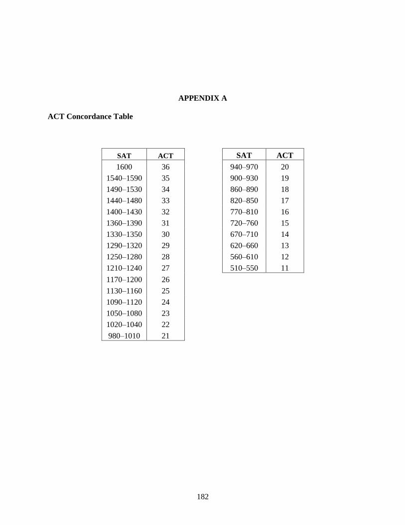
182
APPENDIX A
ACT Concordance Table
SAT ACT
SAT ACT
1600 36
940–970 20
1540–1590 35
900–930 19
1490–1530 34
860–890 18
1440–1480 33
820–850 17
1400–1430 32
770–810 16
1360–1390 31
720–760 15
1330–1350 30
670–710 14
1290–1320 29
620–660 13
1250–1280 28
560–610 12
1210–1240 27
510–550 11
1170–1200 26
1130–1160 25
1090–1120 24
1050–1080 23
1020–1040 22
980–1010 21
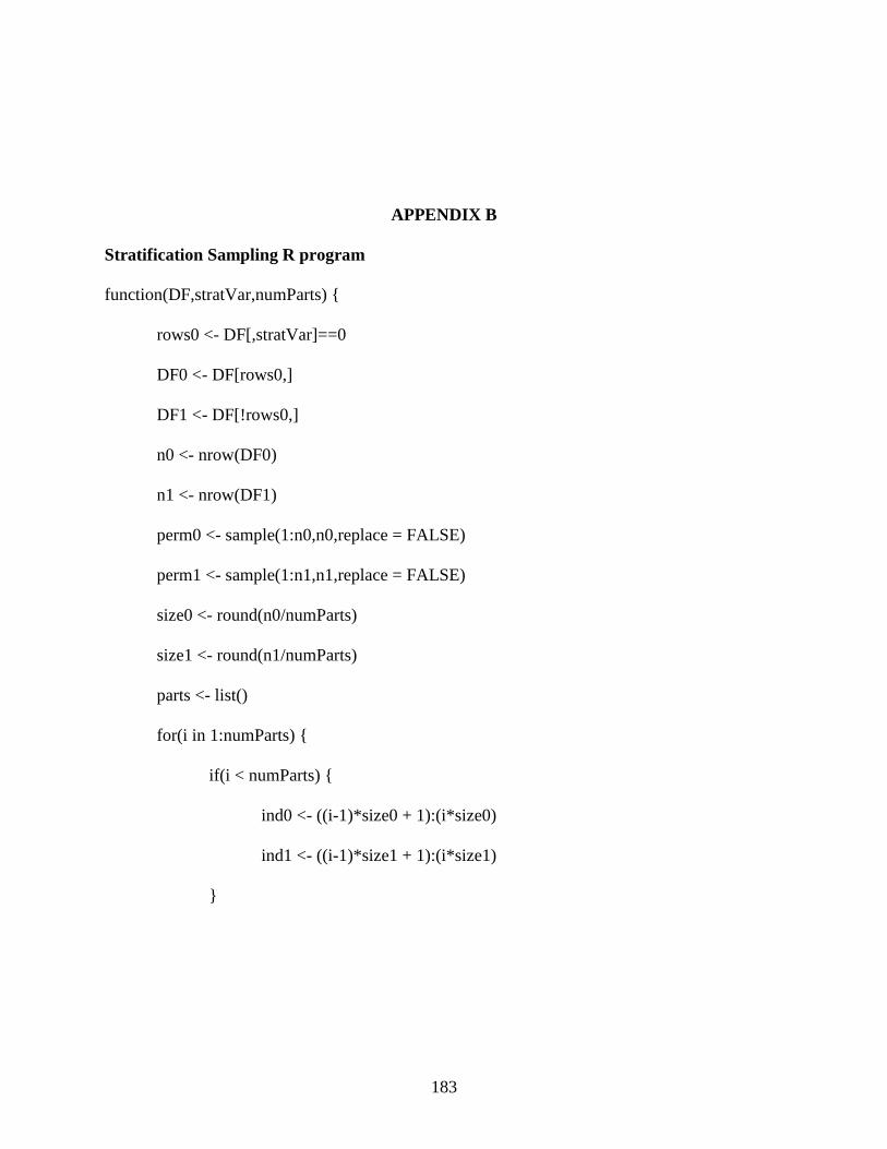
183
APPENDIX B
Stratification Sampling R program
function(DF,stratVar,numParts) {
rows0 <- DF[,stratVar]==0
DF0 <- DF[rows0,]
DF1 <- DF[!rows0,]
n0 <- nrow(DF0)
n1 <- nrow(DF1)
perm0 <- sample(1:n0,n0,replace = FALSE)
perm1 <- sample(1:n1,n1,replace = FALSE)
size0 <- round(n0/numParts)
size1 <- round(n1/numParts)
parts <- list()
for(i in 1:numParts) {
if(i < numParts) {
ind0 <- ((i-1)*size0 + 1):(i*size0)
ind1 <- ((i-1)*size1 + 1):(i*size1)
}

184
else {
ind0 <- ((i-1)*size0 + 1):n0
ind1 <- ((i-1)*size1 + 1):n1
}
parts[[i]] <- rbind(DF0[perm0[ind0],],DF1[perm1[ind1],])
}
return(parts)
}

185
Decision Tree Model with n = 10 fold Cross-validation – R program
function(DFparts) {
for(i in 1:10) {
DFtrain <- data.frame()
for(j in 1:10) {
if(j != i) {
DFtrain <- rbind(DFtrain,DFparts[[j]])
}
}
DFtest <- DFparts[[i]][-1,]
tree <- ctree (Graduation ~.,DFtrain)
pred <- predict(tree, DFtest,type="class")
printcp(rtree) # display the results
summary(rtree) # detailed summary of splits
mis <- mean(pred!=DFtest[,"Graduation"])
print(mis)
}
return(mis)
}

186
Neural Network Model with n = 10 fold Cross-validation – R Program
function(DFparts) {
for(i in 1:10) {
DFtrain <- data.frame()
for(j in 1:10) {
if(j != i) {
DFtrain <- rbind(DFtrain,DFparts[[j]])
}
}
DFtest <- DFparts[[i]][-1,]
nn <- neuralnet (Graduation~HSENG,DFtrain)
pred <- predict(tree, DFtest,type="class")
printcp(rtree) # display the results
summary(rtree) # detailed summary of splits
mis <- mean(pred!=DFtest[,"Graduation"])
print(nn)
}
return(mis)
}

187
Logistic Regression Model with n = 10 fold Cross-validation – R Program
function(DFparts) {
for(i in 1:10) {
DFtrain <- data.frame()
for(j in 1:10) {
if(j != i) {
DFtrain <- rbind(DFtrain,DFparts[[j]])
}
}
DFtest <- DFparts[[i]]
Reg <- regsubsets(Graduation ~., DFtrain)
pred <- predict(Reg, DFtest,type="response")
mis <- mean({pred > 0.5} != {DFtest[,"Graduation"] == "Y"})
print(summary(mis))
}
return(mis)
}

188
Random Forests Model with n = 10 fold Cross-validation – R Program
function(DFparts) {
for(i in 1:10) {
DFtrain <- data.frame()
for(j in 1:10) {
if(j != i) {
DFtrain <- rbind(DFtrain,DFparts[[j]])
}
}
DFtest <- DFparts[[i]][-1,]
tree <- randomForest (Graduation ~.,DFtrain)
pred <- predict(tree, DFtest,type="class")
#printcp(rtree) # display the results
#summary(rtree) # detailed summary of splits
mis <- mean(pred!=DFtest[,"Graduation"])
print(mis)
}
return(mis)
}