Predicting Surface Heat Flux and Temperature via a Pulse

University of Tennessee, Knoxville University of Tennessee, Knoxville

TRACE: Tennessee Research and Creative TRACE: Tennessee Research and Creative

Exchange Exchange

Masters Theses Graduate School

5-2020

Predicting Surface Heat Flux and Temperature via a Pulse-Echo Predicting Surface Heat Flux and Temperature via a Pulse-Echo

Acoustic Transducer for Inverse Heat Conduction Applications Acoustic Transducer for Inverse Heat Conduction Applications

Kevin Jiju Mathew University of Tennessee, [email protected]

Follow this and additional works at: https://trace.tennessee.edu/utk_gradthes

Recommended Citation Recommended Citation Mathew, Kevin Jiju, "Predicting Surface Heat Flux and Temperature via a Pulse-Echo Acoustic Transducer for Inverse Heat Conduction Applications. " Master's Thesis, University of Tennessee, 2020. https://trace.tennessee.edu/utk_gradthes/5596

This Thesis is brought to you for free and open access by the Graduate School at TRACE: Tennessee Research and Creative Exchange. It has been accepted for inclusion in Masters Theses by an authorized administrator of TRACE: Tennessee Research and Creative Exchange. For more information, please contact [email protected].

https://trace.tennessee.edu/

https://trace.tennessee.edu/

https://trace.tennessee.edu/utk_gradthes

https://trace.tennessee.edu/utk-grad

https://trace.tennessee.edu/utk_gradthes?utm_source=trace.tennessee.edu%2Futk_gradthes%2F5596&utm_medium=PDF&utm_campaign=PDFCoverPages

mailto:[email protected]

To the Graduate Council:

I am submitting herewith a thesis written by Kevin Jiju Mathew entitled "Predicting Surface Heat

Flux and Temperature via a Pulse-Echo Acoustic Transducer for Inverse Heat Conduction

Applications." I have examined the final electronic copy of this thesis for form and content and

recommend that it be accepted in partial fulfillment of the requirements for the degree of

Master of Science, with a major in Mechanical Engineering.

Jay Frankel, Major Professor

We have read this thesis and recommend its acceptance:

Kivanc Ekici, Zhili Zhang

Accepted for the Council:

Dixie L. Thompson

Vice Provost and Dean of the Graduate School

(Original signatures are on file with official student records.)

Predicting Surface Heat Flux and Temperature via a Pulse-Echo

Acoustic Transducer for Inverse Heat Conduction Applications

A Thesis Presented for the

Master of Science

Degree

The University of Tennessee, Knoxville

Kevin Jiju Mathew

May 2020

ii

ACKNOWLEDGEMENT

I would like to express my deepest and most sincere gratitude to my family, friends,

mentors at The University of Tennessee, colleagues, and Dr. Jay I. Frankel; Thank you

for letting me be the best I can be. Dr. Frankel, thank you being a wonderful teacher and

an excellent graduate advisor. I wish you well in your new venture as the new

Department Head of Mechanical and Aerospace Engineering at New Mexico State

University.

iii

ABSTRACT

Practical heat transfer situations rise where in-depth measurements must be used to

predict a transient surface temperature or heat flux history. These occurrences are

especially evident and necessary when a surface is exposed to a harsh thermal or

chemical environment as the surface mounted sensor would most likely fail or lose its

integrity over time. Unlike direct or forward problems, where the boundary condition is

specified and the task is determining the temperature distribution, the reversed analysis

produces numerous undesirable mathematical features. In particular, a well-posed process

becomes ill-posed during this reversal. Any small error in the measurement leads to

dramatic error amplification of the inverse prediction. This thesis describes an alternative

measurement technique based on ultrasonic interferometry. Classically, in-depth

thermocouples are used that require holes to be drilled into the sample. For the proposed

sensor scenario, the sensor is mounted onto the back-side (passive side) of the sample and

an ultrasonic pulse is released and timed (round-trip) in the sensor that produces the

pulse. This time-of-flight measurement, using a pulse-echo arrangement, can be

correlated to either surface temperature or heat flux. Regularization, a mathematical

approach for stabilizing ill-posed problems, is introduced based on a future-time concept.

In this approach, a family of predictions is produced based on the chosen regularization

parameter. The most challenging problem associated with inverse problems is the

identification of the optimal prediction. For the present study, a thermal phase plane is

utilized to provide a qualitative view that explicitly shows instability and over-smoothing

of the transient surface condition based on the regularization parameter. For a

quantitative measure or metric, cross-correlation is described and its corresponding phase

plane is used for estimating the optimal prediction, i.e., identification of the optimal

regularization parameter. A numerical study is illustrated demonstrating the methodology

and its accuracy for reconstructing the surface boundary condition.

iv

TABLE OF CONTENTS

Chapter One Introduction ................................................................................................... 1

1.1: Opening Remarks .................................................................................................... 1

Chapter Two Input and data generation .............................................................................. 2

2.1: Introduction .............................................................................................................. 2

2.2: Heat Equation and Auxiliary Conditions ................................................................. 2

2.3: Chosen Surface Heat fluxes for Inverse Study ........................................................ 3

2.4-: Temperature Distribution ....................................................................................... 4

2.5: Time-of-flight .......................................................................................................... 6

2.6: Simulating Noisy Data ........................................................................................... 11

Chapter Three traditional Inverse analysis using future time method .............................. 13

3.1: Introduction ............................................................................................................ 13

3.2: Regularization ........................................................................................................ 13

3.3: Heat Flux................................................................................................................ 13

3.3.1: Family of Predictions Using Perfect Data ...................................................... 17

3.3.2: Family of Predictions Using Real-Life (Noisy) Data ..................................... 20

Chapter Four preconditioned Inverse analysis using future time method ........................ 25

4.1: Introduction ............................................................................................................ 25

4.1.1: Preconditioning ............................................................................................... 25

4.2: Heat Flux................................................................................................................ 25

4.3: Case A: n = 1/2 ..................................................................................................... 26

4.3.1: Family of Predictions Using Noisy Data (Case 2) .......................................... 27

4.3.2: Isolating the Optimal Prediction ..................................................................... 28

4.3.3: Root-Mean Square Error (RMSE) .................................................................. 30

4.4: Case B: n = 3/4 ..................................................................................................... 31

4.4.1: Family of Predictions Using Noisy Data (Case 2) .......................................... 33



4.5: Case C: n = 1 ......................................................................................................... 37

4.5.1: Family of Predictions Using Noisy Data ........................................................ 38



Chapter Five conclusion ................................................................................................... 44

5.1 Conclusions ............................................................................................................. 44

5.2 Future Work ............................................................................................................ 44

References ......................................................................................................................... 46

Appendices ........................................................................................................................ 48

Appendix A ....................................................................................................................... 49

Appendix B ....................................................................................................................... 55

Appendix C: ...................................................................................................................... 59

Appendix D: ...................................................................................................................... 63

Appendix E: ...................................................................................................................... 65

Vita .................................................................................................................................... 68

v

LIST OF TABLES

Table 2.1: Thermophysical properties of stainless steel 304 .............................................. 5

Table 3.1: Root-mean-square experimental error values for traditional inverse analysis 24

Table 4.1: Root-mean-square experimental error values for preconditioned inverse

analysis, case one ...................................................................................................... 31


analysis, case two ...................................................................................................... 37


analysis, Case C using noisy T.o.F data generated for Case 2.................................. 43

vi

LIST OF FIGURES

Figure 2.1: Input flux case 2: single gauss .......................................................................... 3

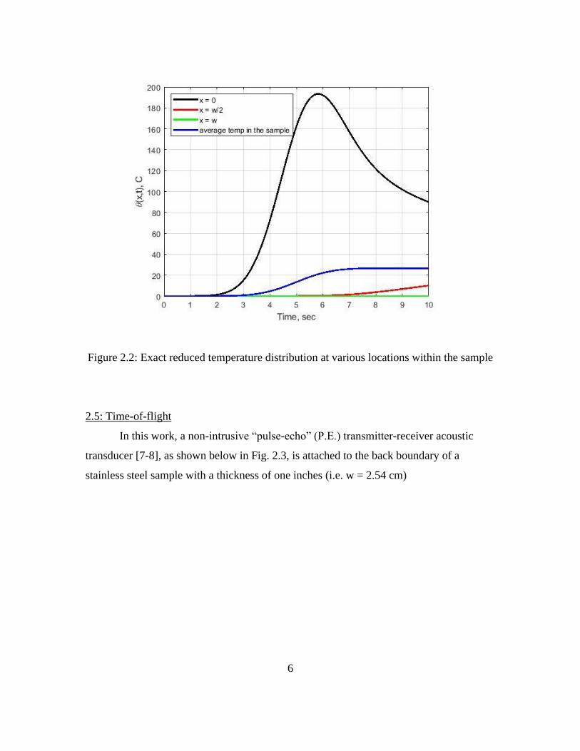
Figure 2.2: Exact reduced temperature distribution at various locations within the sample

..................................................................................................................................... 6

Figure 2.3: Test sample subjected to the boundary conditions with the acoustic sensor

mounted onto the passive side [1] ............................................................................... 7

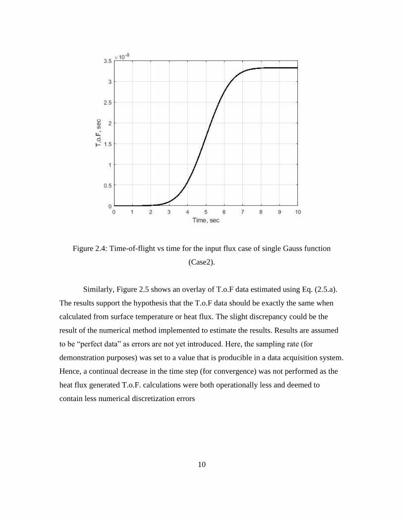
Figure 2.4: Time-of-flight vs time for the input flux case of single Gauss function

(Case2). ..................................................................................................................... 10

Figure 2.5: Time-of-flight data calculated from heat flux and surface temperature to

demonstrate the validity of the governing equations (Case 2) .................................. 11

Figure 2.6: Time-of-flight data calculated from heat flux and perturbed 1 percent of

maximum value to simulate extreme real-life scenario (Case 2) .............................. 12

Figure 3.1: Inverse reconstruction with perfect data (Case 2) .......................................... 17

Figure 3.2: Phase-plane analysis for the inverse analysis with perfect measurement data

(Case 2) ..................................................................................................................... 19

Figure 3.3: Derivative of cross-correlation coefficients vs cross-correlation coefficient

for traditional inverse analysis with perfect measurement data (Case 2) ................. 20

Figure 3.4: Traditional inverse reconstruction with noisy data ........................................ 21

Figure 3.5: Phase-plane analysis for the traditional inverse analysis with noisy

measurement data...................................................................................................... 22


for traditional inverse analysis with noisy measurement data .................................. 23

Figure 4.1: Preconditioned inverse reconstruction, Case A (n = 0.5), with noisy data

(Case 2) ..................................................................................................................... 28

Figure 4.2: Phase-plane analysis for the preconditioned inverse analysis, case one, with

noisy measurement data ............................................................................................ 29

Figure 4.3: Derivative of cross-correlation coefficients vs cross-correlation coefficient for

preconditioned inverse analysis, case one, with noisy measurement data ................ 30

Figure 4.4: Preconditioned inverse reconstruction, case B, with noisy data (case 2) ....... 33

Figure 4.5: Phase-plane analysis for the preconditioned inverse analysis, case B, with

noisy measurement data (Case 2) ............................................................................. 34


preconditioned inverse analysis, Case B, with noisy measurement data (Case 2) ... 35

Figure 4.7: Isolating the optimal prediction for preconditioned inverse analysis, case B,

with noisy measurement data (Case 2) ..................................................................... 36

Figure 4.8: Preconditioned inverse reconstruction, case three, with noisy data ............... 39

Figure 4.9: Phase-plane analysis for the preconditioned inverse analysis, case C, with

noisy measurement data (Case 2) ............................................................................. 40


for preconditioned inverse analysis, case C, with noisy measurement data (Case 2)41

Figure 4.11: Isolating the optimal prediction for preconditioned inverse analysis, case C,

with noisy data (Case 2) ............................................................................................ 42

1

CHAPTER ONE

INTRODUCTION

1.1: Opening Remarks

Quantities such as temperature distribution in a sample and heat flux are important

parameters of interest within the hypersonic and heat transfer community. However,

predicting surface heat flux and temperature in harsh thermal environments requires the

use of inverse heat conduction analysis that removes the need for surface mounted

instrumentation. In-depth measurements protect the integrity of the sensor from harsh or

caustic environments. Inverse analysis generally utilizes in-depth measurements that are

then mathematically projected to the surface based on the classical (parabolic) heat

equation [1]. However, in-depth measurements yield to an “ill-posed” analysis and thus

necessitate regularization [2-4]. In-depth measurements add additional layers of

complexity as the exact probe locations and sensor properties are often estimated. The

analysis becomes even more cumbersome as sampling rate is increased. New

measurements methods are required to be developed to estimate the surface heat flux and

temperature based on external measurements.

It has been demonstrated that a non-intrusive method can be implemented that uses

ultrasonic pulse setting and the time-of-flight (T.o.F) can be retrieved from the

instrumentation. [5-9]. In this context, ultrasonic refers to acoustic waves composed of

frequencies greater than 20 𝑘𝐻𝑧. There are three common instrumentation arrangements

that are used to measure T.o.F.: 1) “through transmission” which places the transmitter

and receiver in opposition; 2) “angle beam” or also known as “pitch-catch” method,

which uses one sensor but requires non-normal surface interactions; and “pulse-echo”

method, which uses one transmitter-receiver sensor placed normal to the surface [1]. The

sensor of choice for this study is pulse-echo as is the most common sensor arrangement

and easier to study in an experimental setting.

2

CHAPTER TWO

INPUT AND DATA GENERATION

2.1: Introduction

In this section, a forward heat conduction problem is produced for generating

artificial data for the later inverse heat conduction simulation process.

2.2: Heat Equation and Auxiliary Conditions

Consider the transient, one-dimensional, constant property, transient heat equation

given as [11]

1

𝛼

𝜕𝜃

𝜕𝑡(𝑥, 𝑡) =

𝜕2𝜃

𝜕𝑥2(𝑥, 𝑡), 𝑥 ∈ [0, 𝑤], 𝑡 0 2.1.a

subject to the boundary conditions

𝑞′′(0, 𝑡) = −𝑘

𝜕𝜃

𝜕𝑥(0, 𝑡) = 𝑞𝑠

′′(𝑡) = ?

2.1.b

𝑞′′(𝑤, 𝑡) = −𝑘𝜕𝜃

𝜕𝑥(𝑤, 𝑡) = 𝑞𝑤

′′(𝑡), 𝑡 ≥ 0 2.1.c

and initial condition

𝜃(𝑥, 0) = 0, 𝑥 ∈ [0, 𝑤] 2.1.d

For the inverse problem, qs′′(t) = ? is sought. This represents the net (conductive)

heat flux. For setting up the data, qs′′(t) is known. The next section describes the surface

heat fluxes chosen for the simulation studies.

3

2.3: Chosen Surface Heat fluxes for Inverse Study

To show the flexibility and adaptability of the method, three input flux cases were

chosen. Case one consisted of a condition where the input flux resembled a step function

with amplitude of 𝐴0 = 100𝑊

𝑐𝑚2. While the option for net heat flux at 𝑥 = 0 is often

challenging to produce in real-life scenarios, it was considered because it can be easily

modeled and represents a challenging reconstruction due to discontinuities (on-off).

Case two, for the input net heat flux, was a Gaussian function with amplitude of

𝐴0 = 100𝑊

𝑐𝑚2 as shown in Figure 2.1. This case was chosen as it resembles a typical

atmospheric maneuver for a high-speed flight vehicle. Case three is a double Gaussian

function reflecting that of a complex maneuver that a flight vehicle might encounter

during a long-term gliding event. The data from these input conditions will be used in the

inverse analysis to accurately reconstruct surface heat flux. Case featuring the single

Gauss will be the input flux case that is extensively described throughout this work.

Figure 2.1: Input flux case 2: single gauss

4

2.4-: Temperature Distribution

The temperature distribution in a sample is also of great interest within the

hypersonic community. Let (𝑥, 𝑡) be defined as the reduced temperature and given

as 𝑇(𝑥, 𝑡) = (𝑥, 𝑡) + 𝑇𝑜. Assuming 𝑞′′(0, 𝑡) is known, the exact temperature

distribution at any point 𝑥 in space within the sample, see Appendix A for derivation, can

be obtained as

𝜃(𝑥, 𝑡) =𝛼

𝑘∑

𝜓𝑚(𝑥)

𝑁𝑚∫ 𝑞′′(𝑢)𝑒−𝛼𝜆𝑚

2 (𝑡−𝑢) 𝑑𝑢𝑡

𝑢=0

, 𝑥 ∈ [0, 𝑤], 𝑡 0

∞

𝑚=0

2.2.a

where 𝜓𝑚(𝑥) is the mth eigenfunction defined as

𝜓𝑚(𝑥) = cos(𝜆𝑚𝑥), 𝑚 = 0,1, … , ∞ 2.2.b

and where 𝜆𝑚 defines the mth eigenvalue as

𝜆𝑚 =𝑚𝜋

𝑤 , 𝑚 = 0,1, … , ∞ 2.2.c

with the mth normalization integral, 𝑁𝑚, defined as

𝑁𝑚 = {

𝑤, 𝑚 = 0

𝑤

2, 𝑚 = 1,2, … , ∞

2.2.d

The temperature profile at any location in the slab subject to some prescribed

surface heat flux condition is now available. Figure 2.2 shows the temperature histories

produced by the previously described single Gauss heat flux. Table 2.1 contains the

thermophysical properties used for this simulation (stainless steel 304) [12-15].

5

Table 2.1: Thermophysical properties of stainless steel 304

Property Value

Thermal conductivity, 𝑘 14.7 (W/m-K)

Density, 𝜌 6861 (kg/m3)

Specific heat, 𝐶𝑝 571.345 (J/kg-K)

Speed of sound at room temperature 5750 (m/s)

Coefficient of linear expansion, 𝛽 17.6 x 10-6 (m/m-K)

Using a Gaussian function as the input case for surface heat flux, it can be

observed, from Figure 2.2, that the maximum reduced surface temperature (active side) at

𝑥 = 0 is roughly 195°𝐶. For the single region problem defined in Figure 2.3, the sensor

(passive) side must remain cool enough to not corrupt or damage the sensor (max 50°𝐶).

From Figure 2.2, the temperature at the back boundary defined as x=w (passive side)

where the acoustic transducer is located, is roughly 0°𝐶. This simple analysis allows for

using this type of sensor for the heat flux and time span indicated without damage

concerns to the sensor.

Should there be need for these instruments be used in scenarios where the back

boundary temperature exceeds the recommended maximum value, adding an insulator

(buffer layer between sample material and transducer) material such as quartz can then

allow for those applications to be considered.

6

Figure 2.2: Exact reduced temperature distribution at various locations within the sample

2.5: Time-of-flight

In this work, a non-intrusive “pulse-echo” (P.E.) transmitter-receiver acoustic

transducer [7-8], as shown below in Fig. 2.3, is attached to the back boundary of a

stainless steel sample with a thickness of one inches (i.e. w = 2.54 cm)

7

Figure 2.3: Test sample subjected to the boundary conditions with the acoustic sensor

mounted onto the passive side [1]

The P.E. acoustic transducer used in this analysis sends a

longitudinal/compressional wave from the passive side to the active side and the reflected

signal is collected at the passive side using the receiver [1]. The speed of sound in solids

depends on various mechanical properties such as Young’s modulus, bulk modulus, shear

modulus, and density for elastic materials. These mechanical properties are usually

temperature dependent. The local speed of sound can be estimated using these properties

and expressed as a function of reduced temperature, 𝜃(𝑥, 𝑡). From Frankel and Bottländer

[1], this relationship is

∫ 𝜃(𝑥, 𝑡)𝑑𝑥𝑤

𝑥=0

= 𝜆𝑜[𝐺 ̃(𝑡) − 𝐺0] 2.3.a

𝜆𝑜 = 𝑐(𝑇0)

2{𝛽0−[1

𝑐(𝑇0)]

𝑑𝑐

𝑑𝑇|𝑇0

2.3.b

8

where 𝐺(𝑡) ≈ �̃�(𝑡) is the time-of-flight variable, 𝜆𝑜 is called the acoustic

parameter, 𝑐(𝑇0) is the speed of sound evaluated at the initial condition 𝑇0, 𝛽0 is the

linear thermal expansion coefficient at the initial condition 𝑇0. As pointed out by Frankel

and Bottländer [1], �̃�(𝑡) approximates 𝐺(𝑡) due to series truncation.

The uniqueness of this work revolves around the use of time-of-flight (T.o.F.) as

the single and only input required to determine both the surface heat flux and surface

temperature. During many practical applications, this will be the only data that is

measured using the P.E. acoustic transducer. This measured data form, unlike locally

measured values obtained by heat flux or temperature gauges, is obtained as a global

averaged value within the sample. Thermocouples are often located in-depth (away from

the active boundary) and since signal penetration is a function of time, there is a physical

delay associated with this measurement technique. This delay in measurement, while

using a TC, can be substantially lessened when using an acoustic transducer as the

measurement device.

As mentioned above, the P.E. configuration directly measures T.o.F which can be

correlated to heat flux and surface temperature through an energy balance. Using Eq.

(2.1.a) and a forward solution of the heat equation, which assumes that 𝑞′′(0, 𝑡) is

known, we can manipulate the analysis and estimate the heat flux from the T.o.F data as

[1]

∫ 𝑞𝑠′′(𝑢)𝑘𝑞(𝑡 − 𝑢)𝑑𝑢

𝑡

𝑢=0

= 𝜆𝑜 (𝑘

𝛼) ∆�̃�(𝑡) 2.4.a

where the convolution kernel, 𝑘𝑞(𝑡 − 𝑢) in Eq. (2.4.a) is defined as

𝑘𝑞(𝑡 − 𝑢) = 1 2.4.b

Here 𝜆𝑜 is the acoustic parameter [1] defined in Eq. (2.3.b), 𝑘 is the thermal conductivity,

and 𝛼 is the thermal diffusivity of the material. The derivation of Eq. (2.4.a) is worked

out in extensive detail in Appendix B.

9

Similarly, it can be shown that if the interest is in seeking surface temperature

(instead of heat flux as shown in Eq. (2.4.a)), then the measurement equation becomes

∫ 𝜃(0, 𝑢)𝑘𝑇(𝑡 − 𝑢)𝑑𝑢 = 𝑓(𝑡)𝑡

𝑢=0

2.5.a

where the convolution kernel, 𝑘𝑇(𝑡 − 𝑢) in Eq. (2.5.a) is defined as

𝑘𝑇(𝑡 − 𝑢) =1

√𝑡 − 𝑢∑(−1)𝑗 {𝑒

(−(2𝑤𝑗)2

4𝛼(𝑡−𝑢))

− 𝑒(

−(2𝑤(𝑗+1))2

4𝛼(𝑡−𝑢))

}

∞

𝑗=0

2.5.b

with the resulting forcing function, 𝑓(𝑡) defined as

𝑓(𝑡) =√𝜋𝜆𝑜

√𝛼[𝐺(𝑡) − 𝐺0] 2.5.c

where 𝐺0 is the T.o.F at the uniform initial condition. The derivations of Eq. (2.5.a), Eq.

(2.5.b), and Eq. (2.5.c) are worked out in extensive detail in Appendix C.

At this junction, T.o.F data are numerically generated for the present

investigation. The major contribution of this study is to demonstrate a viable

methodology for estimating surface heat flux and temperature. Algebraic manipulations

to Eq. (2.4.a) and Eq. (2.5.a) yield the expression which can be solved to numerically

generate the T.o.F data. Once the expression for T.o.F is obtained, it can be discretized

and the definite integral can be numerically approximated using a trapezoidal rule. To

validate the governing equations, Eq. (2.4.a) and Eq. (2.5.a) were both numerically

solved as they should yield the same T.o.F data. Figure 2.4, estimated using Eq. (2.4.a),

shows the T.o.F behavior as a function of time for the prescribed input flux condition.

10

Figure 2.4: Time-of-flight vs time for the input flux case of single Gauss function

(Case2).

Similarly, Figure 2.5 shows an overlay of T.o.F data estimated using Eq. (2.5.a).

The results support the hypothesis that the T.o.F data should be exactly the same when

calculated from surface temperature or heat flux. The slight discrepancy could be the

result of the numerical method implemented to estimate the results. Results are assumed

to be “perfect data” as errors are not yet introduced. Here, the sampling rate (for

demonstration purposes) was set to a value that is producible in a data acquisition system.

Hence, a continual decrease in the time step (for convergence) was not performed as the

heat flux generated T.o.F. calculations were both operationally less and deemed to

contain less numerical discretization errors

11

.

Figure 2.5: Time-of-flight data calculated from heat flux and surface temperature to

demonstrate the validity of the governing equations (Case 2)

2.6: Simulating Noisy Data

Data generated up to this junction are assumed perfect, but that condition is rarely

obtainable in real-world data collection which normally involves random and bias errors.

Numerically articulated noise should have these components, but bias errors are normally

removed whenever possible. Hence, this study will only consider random errors. Thus, to

simulate real-life scenarios, the perfect data generated from above was randomly

perturbed about the maximum value per Figure 2.6. Perturbing about the maximum value

was selected as this an extreme case, if the inverse analysis can produce stable

predictions to this highly noisy condition, then it can be concluded that this approach is

compatible to handle complex scenarios.

12

Figure 2.6: Time-of-flight data calculated from heat flux and perturbed 1 percent of

maximum value to simulate extreme real-life scenario (Case 2)

13

CHAPTER THREE

TRADITIONAL INVERSE ANALYSIS USING FUTURE TIME

METHOD

3.1: Introduction

Inverse problems are prevalent in all branches of physics and engineering. The

use of surface mounted sensors is often discouraged in many applications as they may not

survive a harsh thermal environment. Examples include development of thermal

protection systems (TPS) used in the aerospace industry; study of advanced high-

temperature materials; and, in the understanding fire and fusion technology. This

limitation can be resolved by using in-depth or backside sensors. These sensor

orientations protect the integrity of the probe when they are subjected to hostile

conditions to predict surface conditions such as heat flux or temperature. This approach,

however, leads to an analysis that is highly ill posed as small errors from the collected

discontinuous data leads to dramatic error amplification in the prediction of either surface

heat flux or temperature [16].

3.2: Regularization

Equations (2.4.a) and (2.5.a) are first kind Volterra integral equations and as such

they require careful analysis to find stable/regularized and accurate predictions.

Many regularization methods are available including Singular-Value Decomposition

(SVD), Tikhonov Regularization, Digital Filtering, Future time method etc [16]. These

methods can produce predictions to some level of accuracy. In this study, inverse analysis

is performed through future time method. The crucial part of inverse problem is to

scientifically and methodically acquire the optimal regularization parameter; This method

is further explained in detail in this chapter.

3.3: Heat Flux

As mentioned earlier, Eq. (2.4.a) is a first kind Volterra integral equation [1]. To

stabilize this highly ill-posed equation, a regularization parameter, 𝛾 must be interjected

14

into the formulation for stabilizing the proposed numerical method for resolving the

surface boundary condition. For the present work, we introduce the notation of future

time which serves as the regularization parameter. To begin, we let 𝑡 → 𝑡 + 𝛾 into Eq.

(2.4a) to obtain

∫ 𝑞𝑠′′(𝑢)𝑘𝑞(𝑡 + 𝛾 − 𝑢)𝑑𝑢

𝑡+𝛾

𝑢=0

= 𝜆𝑞∆�̃�(𝑡 + 𝛾) , 𝑡 ≥ 0 3.1.a

where 𝜆𝑞 is defined as

𝜆𝑞 = 𝜆𝑜 (𝑘

𝛼) 3.1.b

Separating the “forward time region’’ in the integral representation yields

𝜆𝑞∆�̃�(t + 𝛾) = ∫ 𝑞𝑠′′(𝑢)𝑘𝑞(𝑡 + 𝛾 − 𝑢)𝑑𝑢

𝑡

𝑢=0

+ ∫ 𝑞𝑠′′(𝑢)𝑘𝑞(𝑡 + 𝛾 − 𝑢)𝑑𝑢

𝑡+𝛾

𝑢=𝑡

3.1.c

As specified above, future-time will help stabilize the analysis by holding the heat

flux fixed in the future time interval, [𝑡, 𝑡 + ] . This transforms the ill-posed first kind

Volterra integral equation to a well-posed second kind Volterra integral equation; namely

𝜆𝑞∆�̃�(𝑡 + 𝛾) ≅ ∫ 𝑞𝑠′′(𝑢)𝑘𝑞(𝑡 + 𝛾 − 𝑢)𝑑𝑢

𝑡

𝑢=0

+ 𝑞𝑠′′(𝑡) ∫ 𝑘𝑞(𝑡 + 𝛾 − 𝑢)𝑑𝑢

𝑡+𝛾

𝑢=𝑡

3.1.d

Next, we introduce the first in a series of approximations as

15

𝑞𝑠′′(𝑢) ≅ 𝑞𝑠

′′(𝑡) , 𝑢 ∈ [𝑡, 𝑡 + 𝛾] 3.1.e

Next, we move from the continuous time domain to the discrete time domain in Eq.

(3.1.d), by letting 𝑡 → 𝑡𝑖 and hence 𝛾 → 𝛾𝑚

𝜆𝑞∆�̃�(𝑡𝑖 + 𝛾𝑚) ≅

∫ 𝑞𝑠′′(𝑢)𝑘𝑞(𝑡𝑖 + 𝛾𝑚 − 𝑢)𝑑𝑢

𝑡𝑖

𝑢=0

+ 𝑞𝑠′′(𝑡𝑖 ) ∫ 𝑘𝑞(𝑡𝑖 + 𝛾𝑚 − 𝑢)𝑑𝑢

𝑡𝑖 +𝛾𝑚

𝑢=𝑡𝑖

𝑖 = 1,2, … , 𝑁 − 𝑚𝑀𝑓 , 𝑚 = [1,2,3,4,5,6,7]

3.1.f

where 𝑀𝑓 is a scalar multiplying factor, in this study 𝑀𝑓 = 5, to reasonably scale the

future-time parameter, 𝛾𝑚, defined as

𝛾𝑚 = 𝑚𝑀𝑓∆𝑡 3.1.g

and 𝑡𝑖 in Eq. (3.1.f) is defined as

𝑡𝑖 = (𝑖 − 1)∆𝑡, 𝑖 = 1,2, … , 𝑁 3.1.h

where N equals the total number of data collected and ∆𝑡 is defined as

∆𝑡 = 𝑡𝑚𝑎𝑥

𝑁 − 1 3.1.i

The definite integrals defined in Eq. (3.1.f) can be approximated using a single panel

approximation (i.e., trapezoidal) as

16

𝜆𝑞∆�̃�(𝑡𝑖 + 𝛾𝑚) ≅ ∑ ∫ 𝑞𝑠

′′(𝑢)𝑘𝑞(𝑡𝑖 + 𝛾𝑚 − 𝑢)𝑑𝑢𝑡𝑗+1

𝑢=𝑡𝑗

𝑖−1

𝑗=1

+ 𝑞𝑠′′(𝑡𝑖 )𝐶𝛾𝑚

,

𝑖 = 1,2, … , 𝑁

3.1.j

where 𝐶𝛾𝑚 is defined as

𝐶𝛾𝑚= ∫ 𝑘𝑞(𝑡𝑖 + 𝛾𝑚 − 𝑢)𝑑𝑢

𝑡𝑖 +𝛾𝑚

𝑢=𝑡𝑖

3.1.k

Next, release the last panel in the numerical approximation to create additional stability.

This leads to the intermediate formulation

𝜆𝑞∆�̃�(𝑡𝑖 + 𝛾𝑚) ≅ ∑ ∫ 𝑞𝑠′′(𝑢)𝑘𝑞(𝑡𝑖 + 𝛾𝑚 − 𝑢)𝑑𝑢

𝑡𝑗+1

𝑢=𝑡𝑗

𝑖−2

𝑗=1

+𝑞𝑠′′(𝑡𝑖) ∫ 𝑘𝑞(𝑡𝑖 + 𝛾𝑚 − 𝑢)𝑑𝑢

𝑡𝑖

𝑢=𝑡𝑖−1

+ 𝑞𝑠′′(𝑡𝑖 )𝐶𝛾𝑚

3.1.l

After some additional algebraic manipulations, we obtain

�̃�𝑠′′(𝑡𝑖) =

𝜆𝑞∆�̃�(𝑡𝑖 + 𝛾𝑚) − ∑ ∫ �̃�𝑠′′(𝑢)𝑘𝑞(𝑡𝑖 + 𝛾𝑚 − 𝑢)𝑑𝑢

𝑡𝑗+1

𝑢=𝑡𝑗

𝑖−2𝑗=1

𝐶𝛾𝑚+ ∫ 𝑘𝑞(𝑡𝑖 + 𝛾𝑚 − 𝑢)𝑑𝑢

𝑡𝑖

𝑢=𝑡𝑖−1

3.1.m

where �̃�𝑠′′(𝑡𝑖) ≅ 𝑞𝑠

′′(𝑡𝑖), 𝑖 = 1,2, . . , 𝑀.

As evident from the final data reduction equation, the present form requires little

numerical processing for resolving the heat flux than many traditional approaches.

17

3.3.1: Family of Predictions Using Perfect Data

As mentioned earlier, inverse analysis provides a family of predictions based on

the regularization parameter’s value. A key to quality estimation is the ability to identify

the optimal prediction that minimizes the error (which is unknown). As error in the input

increases, the inverse analysis becomes highly ill-posed. To illustrate this concept,

consider the traditional inverse analysis with perfect data (no noise. There are nearly an

infinite number of values that can be used as the future time parameter. In this study,

seven such values were considered, 𝑚 = [1,2,3,4,5,6,7]. The goal is to extract the value

of the regularization parameter that can produce the minimum error. Thus, extracting this

optimal value represents the challenge for all inverse methods. Figure 3.1 displays the

family of heat flux predictions for Case 2. It is evident that for large that over-

smoothing effects are observed.

Figure 3.1: Traditional inverse reconstruction with perfect data (Case 2)

18

3.3.1.1: Isolating the Optimal Prediction

The uniqueness of this study is selecting the optimum regularization parameter

from the provided set of choices. To visually and mathematically select the optimum

value, this study applies a combination of phase-plane and cross-correlation analyses to

the prediction family in order to estimate the optimal regularization parameter and hence

the optimal heat flux prediction. Figure 3.2 represents the phase plane analysis for the

reconstruction represented in Figure 3.1. Phase plane analysis presents a visual aid in

identifying the optimal prediction. When the phase-plane prediction, for fixed

regularization parameter, begins to form a pattern or shape, it can be assumed that one is

near the optimal prediction.

Figure 3.3 shows the relationship between derivative of the cross-correlation

coefficients, �̇�, plotted with respect to the cross-correlation coefficient 𝜌. Cross-

correlation is the measure of similarity between two series data streams. This is also

known as a sliding dot product or sliding inner product [16]. Normalized expression for

cross-correlation can be defined as

𝜌1,2(𝑗) =

1𝑁

∑ 𝑥1(𝑛)𝑥2(𝑛)𝑁−1𝑛=0

1𝑁

[∑ 𝑥12(𝑛) ∑ 𝑥2

2(𝑛)𝑁−1𝑛=0

𝑁−1𝑛=0 ]

12

3.2

19

Figure 3.2: Phase-plane analysis for the inverse analysis with perfect measurement data

(Case 2)

Cross-correlation provides a mathematical basis or metric on how to identify the optimal

regularization parameter. The phase plane presentation displayed in Fig. 3.2 provides a

visual aid that is highly helpful. As evident by Figures 3.2 and Fig. 3.3 below, phase

plane and cross-correlation analyses do not strongly aid in finding the optimal future time

prediction when in the presence of perfect measurement data

20


for traditional inverse analysis with perfect measurement data (Case 2)

3.3.2: Family of Predictions Using Real-Life (Noisy) Data

To simulate more physically correct conditions, random noise (approximately one

percent) is added to the T.o.F data sampled at a frequency of 100 𝐻𝑧. The random noise

added is one percent of the maximum value. This condition was considered as the worst-

case scenario. Inverse analysis is performed using Eq. (3.1.m). Figure 3.4 displays the

heat flux predictions based on the displayed future-time parameters. That is, small future-

time parameters show instability while large future time parameters show over-smoothing

effects.

21

Figure 3.4: Traditional inverse reconstruction with noisy data

3.3.2.1: Isolating the Optimal Prediction (Noise)

Identifying optimal predictions from a family of inverse reconstructions is not

trivial as the error in the calculations adds additional complications. Figure 3.5 shows the

phase plane of traditional reconstructions involving noisy data. Figure 3.5 does not

display the formation of a clear pattern. This is indicative of insufficient filtering

somewhere in the methodology. The phase plane and cross-correlation tools previously

described may have difficulties at the present level of analysis.

22

Figure 3.5: Phase-plane analysis for the traditional inverse analysis with noisy

measurement data

To further illustrate the limitations of the traditional or pedestrian formulation,

consider Figure 3.6 which plots the time derivative cross-correlation coefficients versus

the cross-correlation coefficients. While the results are moving to the top-right corner as

expected, this method shows no correlation between the families of predictions. As a

result, the optimal prediction cannot be isolated.

23


for traditional inverse analysis with noisy measurement data

3.3.2.2: Error Analysis (Root-Mean Square Error, RMSE)

Root-mean-square experimental error for the traditional formulation provides a

qualitative view on the prevalence of error in this methodology. Again, in real

experiments, the RMSE does not exist. Table 3.1 highlights these values and shows the

basic effect of an inverse analysis. That is, the RMSE decreases with increasing

regularization parameter up to a point but then the NMSE increases with increasing

regularization parameter. Finding a method that identifies this minimum values is key to

inverse analysis.

24

Table 3.1: Root-mean-square experimental error values for traditional inverse analysis

M 𝜸𝒎(s) Traditional analysis

(W/m2)

1 0.05 139299.2670

2 0.1 80124.8238

3 0.15 57237.1894

4 0.2 46254.3707

5 0.25 41012.4123

6 0.3 39126.1807

7 0.35 39381.3406

25

CHAPTER FOUR

PRECONDITIONED INVERSE ANALYSIS USING FUTURE TIME

METHOD

4.1: Introduction

As demonstrated in Chapter 3, when attempting to perform inverse analysis on

measurement data with noise, the traditional or pedestrian formulation fails to define a

strong method for identifying the optimal regularization parameter based on the proposed

phase-plane and cross-correlation tools. This chapter aims to propose an alternative

integral formulation for prior to using the identification tools (phase plane and cross

correlation) described in Chapter 3. It will be demonstrated that preconditioning the

formulation permits a means for identifying the optimal regularization parameter using

the tools of Chapter 3. Further, the numerical implementation still remains simple and

intuitive.

4.1.1: Preconditioning

Several attractive features will be demonstrated for the newly proposed

preconditioned method for inverse analysis. The soon to be described preconditioner will

act as a parameter-free, low-pass filter providing enough information to utilize phase

plane and cross correlation for identifying the optimal future time parameter.

4.2: Heat Flux

The preconditioner concept will be developed in the context of heat flux per the

formulation proposed in Eq. (2.4.a). This equation, once converted to the frequency

domain using Laplace Transform, is multiplied by 1

𝑆𝑛 to get the desired amount of

filtering. As is evidenced from this study, the filtering operation is applied to the

governing equation rather than to the measured T.o.F. data. In this way, the equality sign

is retained in the conservation of energy. The value of 𝑛, or the attenuation factor,

determines the amount of filtering that is applied to the equation.

26

4.3: Case A: n = 1/2

To begin, take the Laplace Transform to Eq. (2.4.a) as

ℒ{∆𝐺(𝑡)} =1

𝜆𝑞 ℒ {∫ 1 ∙

𝑡

𝑢=0

𝑞𝑠′′(𝑢) 𝑑𝑢} 4.1.a

After Laplace Transform is applied, the above equation becomes

𝜆𝑞∆�̂� = 𝑞𝑠′′̂(𝑠) ∙

1

𝑠 4.1.b

Next, multiply both sides by 1

𝑆(1/2) to obtain

𝜆𝑞∆�̂�

𝑠(12

)= 𝑞𝑠

′′̂(𝑠) ∙1

𝑠(32

) 4.2

Taking the inverse Laplace Transform of Eq. (4.2) ([17] p. 1022 Eq. (29.3.4) and Eq.

(29.3.5)) yields

𝜆𝑞 ∫∆𝐺(𝑢)

√𝜋(𝑡 − 𝑢)𝑑𝑢 = ∫ 𝑞𝑠

′′(𝑢) 2√𝑡 − 𝑢

√𝜋𝑑𝑢

𝑡

𝑢=0

𝑡

𝑢=0

, 𝑡 ≥ 0 4.3

For the case of 𝑛 =1

2, the filtered equation takes the form of Eq. (4.3). The future-time

method is applied to Eq. (4.3). The final data reduction equation can be expressed simply

as

�̃�𝑠′′(𝑡𝑖) =

𝐴 − 𝐵

𝐶 + 𝐷, 𝑖 = 2,3, … , 𝑁 − 𝑚𝑀𝑓 4.4.a

27

where the function 𝐴 is defined as

𝐴 = 𝜆𝑞

2∑ ∫

∆�̃�(𝑢)

√(𝑡𝑖 + 𝛾𝑚 − 𝑢)𝑑𝑢

𝑡𝑗+1

𝑢=𝑡𝑗

𝑖+𝑚𝑀𝑓−1

𝑗=1

4.4.b

function B is defined as

𝐵 = ∑ ∫ 𝑞𝑠′′(𝑢)√(𝑡𝑖 + 𝛾𝑚 − 𝑢)𝑑𝑢

𝑡𝑗+1

𝑢=𝑡𝑗

𝑖−2

𝑗=1

4.4.c

function C is defined as

𝐶 = ∫ √(𝑡𝑖 + 𝛾𝑚 − 𝑢)𝑑𝑢𝑡+𝛾

𝑢=𝑡

4.4.d

And function D is defined as

𝐷 = ∫ √(𝑡𝑖 + 𝛾𝑚 − 𝑢)𝑑𝑢𝑡𝑖

𝑢=𝑡𝑖−1

4.4.e

4.3.1: Family of Predictions Using Noisy Data (Case 2)

Similar to the traditional or pedestrian formulation, this analysis was performed

on noisy data sampled at a sampling frequency at 100 𝐻𝑧. The preconditioned inverse

analysis was performed for reconstructing the surface heat flux using Eq. (4.4.a). Figure

4.1 shows the effect on the heat flux predictions using the previously defined future time

parameters. The jump toward stability is highlighted when using this value of n=1/2 in

the preconditioner.

28

Figure 4.1: Preconditioned inverse reconstruction, Case A (n = 0.5), with noisy data

(Case 2)

4.3.2: Isolating the Optimal Prediction

Although this case was successful in reducing the error bandwidth in the final ill-

posed reconstruction, the main objective of any inverse analysis is to isolate the optimal

prediction from the family of predictions. Figure 4.2 displays the resulting phase plane

analysis for Case A using the data generated by Case 2 heat flux. The attenuation factor

for this case was not effective in isolating the optimal prediction. Figure 4.3 further

solidifies this claim as the cross-correlation phase plane plot fails to show strong

correlation between the families of predictions.

29

Figure 4.2: Phase-plane analysis for the preconditioned inverse analysis, case A, with

noisy measurement data (Case 2)

30


preconditioned inverse analysis, case A, with noisy measurement data

4.3.3: Root-Mean Square Error (RMSE)

The root-mean-square error for the preconditioned inverse analysis provides

insight on how effective the parameter free preconditioner is in reducing errors. The

resulting analysis still contained non-negligible error, but when compared to Table 3.1,

there is a significant improvement.

31

Table 4.1: Root-mean-square experimental error values for preconditioned inverse, case

A, analysis, (Case 2)

M 𝜸𝒎(s) Preconditioned analysis

(W/m2)

1 0.05 97977.5012

2 0.1 36903.4372

3 0.15 23587.2131

4 0.2 23552.8086

5 0.25 28009.3971

6 0.3 33706.4007

7 0.35 39730.9350

4.4: Case B: n = 3/4

First, we apply the Laplace Transform to Eq. (2.3.a) to get in the form represented

by Eq. (4.1.b). Next, we multiply both sides of Eq. (4.1.b) by 1

𝑆(3/4) to obtain

𝜆𝑞∆�̂�

𝑠(34

)= 𝑞𝑠

′′̂(𝑠) ∙1

𝑠(74

) 4.5

Taking the inverse Laplace Transform of Eq. (4.5) produces

𝜆𝑞 ∫∆𝐺(𝑢)

√𝑡 − 𝑢4

Γ (34)

𝑑𝑢 = ∫ 𝑞𝑠′′(𝑢)

(𝑡 − 𝑢)34

Γ (74)

𝑑𝑢𝑡

𝑢=0

𝑡

𝑢=0

, 𝑡 ≥ 0 4.6.a

where the Γ(𝑥)is the gamma function defined as ([17] p. 255 Eq. (6.1.1))

Γ(𝑥) = ∫ 𝑡𝑥−1𝑒−𝑡∞

0

𝑑𝑡 ℜ𝑒(𝑥) > 0 4.6.b

32

For this case, 𝑛 =3

4, the preconditioned measurement equation takes the form of Eq.

(4.6.a). Following our previously outlined procedure for the regularization process based

on the future time, it can be shown to produce

�̃�𝑠′′(𝑡𝑖) =

𝐴 − 𝐵

𝐶 + 𝐷, 𝑖 = 2,3, … , 𝑁 − 𝑚𝑀𝑓 4.7.a

where the function A is defined as

𝐴 = 𝜆𝑞 ∑ ∫∆�̃�(𝑢)

√𝑡𝑖 + 𝛾𝑚 − 𝑢4 Γ (34)

𝑑𝑢𝑡𝑗+1

𝑢=𝑡𝑗


𝑗=1

4.7.b


𝐵 = ∑ ∫ 𝑞𝑠′′(𝑢)

(𝑡𝑖 + 𝛾𝑚 − 𝑢)34

Γ (74)

𝑑𝑢𝑡𝑗+1

𝑢=𝑡𝑗

𝑖−2

𝑗=1

4.7.c


𝐶 = ∫(𝑡𝑖 + 𝛾𝑚 − 𝑢)

34

Γ (74)

𝑑𝑢𝑡+𝛾

𝑢=𝑡

4.7.d

Function D is defined as

𝐷 = ∫(𝑡𝑖 + 𝛾𝑚 − 𝑢)

34

Γ (74)

𝑑𝑢𝑡𝑖

𝑢=𝑡𝑖−1

4.7.e

33

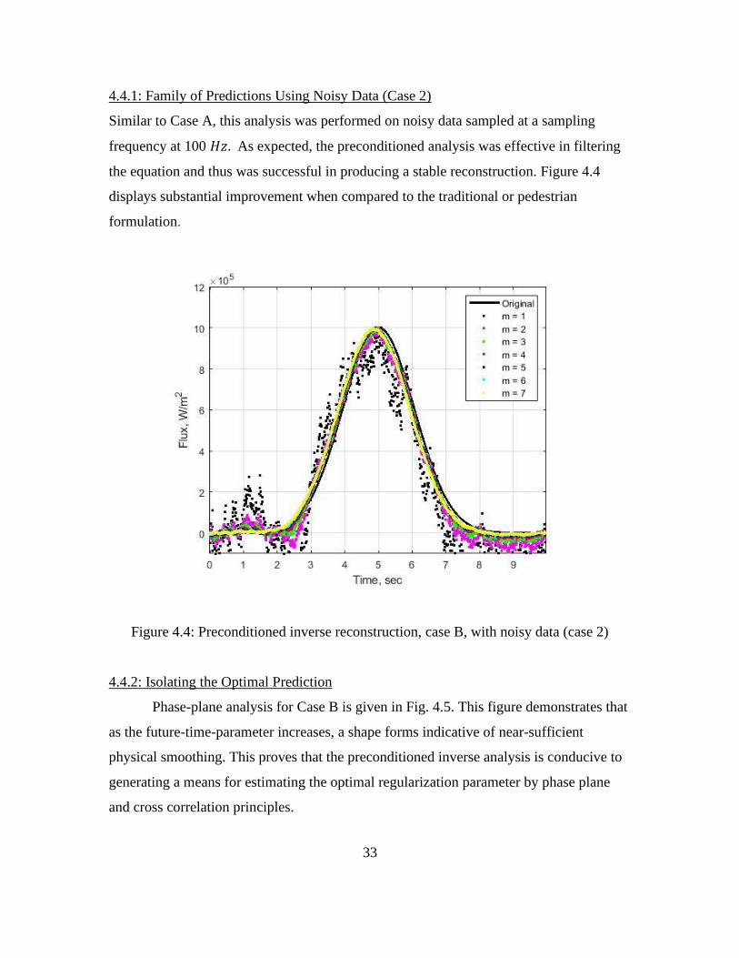
4.4.1: Family of Predictions Using Noisy Data (Case 2)

Similar to Case A, this analysis was performed on noisy data sampled at a sampling

frequency at 100 𝐻𝑧. As expected, the preconditioned analysis was effective in filtering

the equation and thus was successful in producing a stable reconstruction. Figure 4.4

displays substantial improvement when compared to the traditional or pedestrian

formulation.

Figure 4.4: Preconditioned inverse reconstruction, case B, with noisy data (case 2)


Phase-plane analysis for Case B is given in Fig. 4.5. This figure demonstrates that

as the future-time-parameter increases, a shape forms indicative of near-sufficient

physical smoothing. This proves that the preconditioned inverse analysis is conducive to

generating a means for estimating the optimal regularization parameter by phase plane

and cross correlation principles.

34

Figure 4.5: Phase-plane analysis for the preconditioned inverse analysis, case B, with


Figure 4.6 displays the cross-correlation, phase-plane plot indicating an apparent

correlation amongst the family of predictions as the future-time-parameter increases.

Using this estimation, the optimal prediction can be isolated. To isolate the optimal

prediction, based on the cross-correlation, phase-plane plot, the best prediction is located

as both 𝜌 → 1 𝑎𝑛𝑑 𝜌 ̇ → 0.75. Figure 4.7 highlights the optimal heat flux prediction using

highly noisy time-of-flight data.

35


preconditioned inverse analysis, Case B, with noisy measurement data (Case 2)

36

Figure 4.7: Isolating the optimal prediction for preconditioned inverse analysis, case B,

with noisy measurement data (Case 2)


The root-mean-square error for the preconditioned inverse analysis, Case B,

provides quantitative insight on how effective the parameter free preconditioner was on

the noisy time-of-flight data in forming the heat flux approximation for specified future-

time parameter. The attenuation factor was not large enough to effectively reduce the

error completely. However, there is a significant improvement in the overall error

reduction as indicated by comparing Table 3.1 to Table 4.1.

37

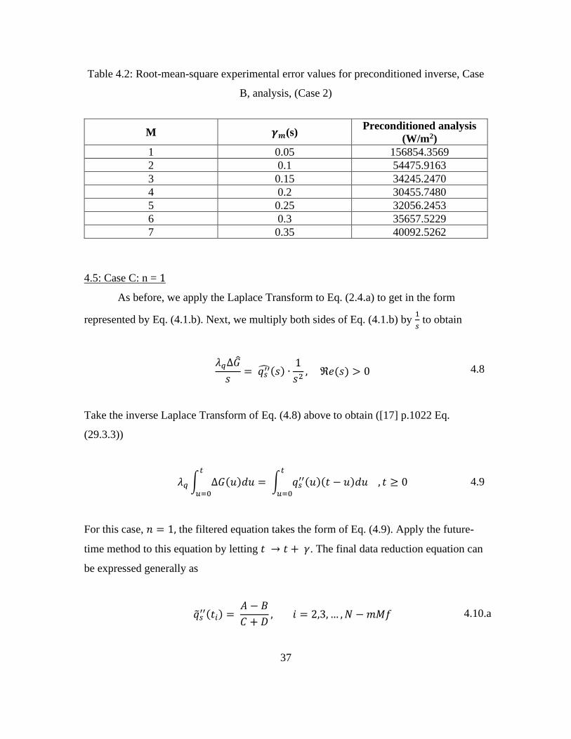
Table 4.2: Root-mean-square experimental error values for preconditioned inverse, Case

B, analysis, (Case 2)


(W/m2)

1 0.05 156854.3569

2 0.1 54475.9163

3 0.15 34245.2470

4 0.2 30455.7480

5 0.25 32056.2453

6 0.3 35657.5229

7 0.35 40092.5262

4.5: Case C: n = 1

As before, we apply the Laplace Transform to Eq. (2.4.a) to get in the form

represented by Eq. (4.1.b). Next, we multiply both sides of Eq. (4.1.b) by 1

𝑠 to obtain

𝜆𝑞∆�̂�

𝑠= 𝑞𝑠

′′̂(𝑠) ∙1

𝑠2, ℜ𝑒(𝑠) > 0 4.8

Take the inverse Laplace Transform of Eq. (4.8) above to obtain ([17] p.1022 Eq.

(29.3.3))

𝜆𝑞 ∫ ∆𝐺(𝑢)𝑑𝑢𝑡

𝑢=0

= ∫ 𝑞𝑠′′(𝑢)(𝑡 − 𝑢)𝑑𝑢 , 𝑡 ≥ 0

𝑡

𝑢=0

4.9

For this case, 𝑛 = 1, the filtered equation takes the form of Eq. (4.9). Apply the future-

time method to this equation by letting 𝑡 → 𝑡 + 𝛾. The final data reduction equation can

be expressed generally as

�̃�𝑠′′(𝑡𝑖) =

𝐴 − 𝐵

𝐶 + 𝐷, 𝑖 = 2,3, … , 𝑁 − 𝑚𝑀𝑓 4.10.a

38

where the function A is defined as

𝐴 = 𝜆𝑞 ∑ ∫ ∆�̃�(𝑢)𝑑𝑢𝑡𝑗+1

𝑢=𝑡𝑗


𝑗=1

4.10.b


𝐵 = ∑ ∫ 𝑞𝑠′′(𝑢)(𝑡𝑖 + 𝛾𝑚 − 𝑢)𝑑𝑢

𝑡𝑗+1

𝑢=𝑡𝑗

𝑖−2

𝑗=1

4.10.c


𝐶 = ∫ (𝑡𝑖 + 𝛾𝑚 − 𝑢)𝑑𝑢𝑡+𝛾

𝑢=𝑡

4.10.d

Function D is defined as

𝐷 = ∫ (𝑡𝑖 + 𝛾𝑚 − 𝑢)𝑑𝑢𝑡𝑖

𝑢=𝑡𝑖−1

4.10.e

4.5.1: Family of Predictions Using Noisy Data

Similar to Cases A, B, this analysis was also performed using noisy time-of-flight

data sampled at a sampling frequency at 100𝐻𝑧. The preconditioned inverse analysis, for

case C, was performed to the measurement data for reconstructing the surface heat flux

using Eq. (4.10.a). Figure 4.8 displays the resulting family of heat flux predictions over

the indicated values of the regularization parameters. When comparing with the results

from the traditional inverse analysis, Cases A and B using the preconditioned method,

Case C has further success in reducing the error bandwidth. The attenuation factor for

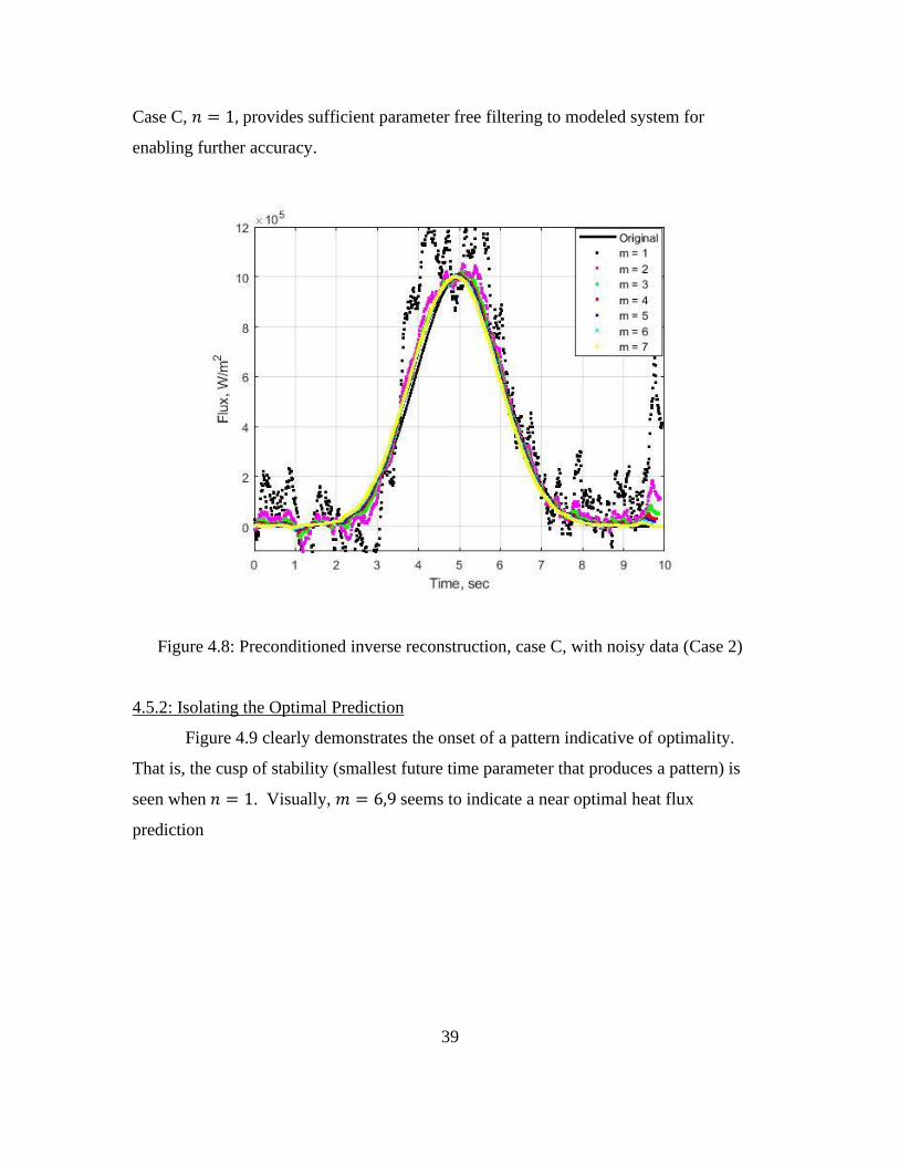
39

Case C, 𝑛 = 1, provides sufficient parameter free filtering to modeled system for

enabling further accuracy.

Figure 4.8: Preconditioned inverse reconstruction, case C, with noisy data (Case 2)


Figure 4.9 clearly demonstrates the onset of a pattern indicative of optimality.

That is, the cusp of stability (smallest future time parameter that produces a pattern) is

seen when 𝑛 = 1. Visually, 𝑚 = 6,9 seems to indicate a near optimal heat flux

prediction

40

Figure 4.9: Phase-plane analysis for the preconditioned inverse analysis, case C, with


Figure 4.10 shows a strong correlation amongst the family of predictions as the

future-time-parameter increases. Here, the future time parameter in the range 0.2 and 0.25

seconds narrows the optimal values. Figure 4.11 highlights the optimal heat flux

prediction for m=4 (4=0.2s) and m=5 (5=0.25s). These results appear superior to Cases

A,B.

41


for preconditioned inverse analysis, case C, with noisy measurement data (Case 2)

42

Figure 4.11: Isolating the optimal prediction for preconditioned inverse analysis, case C,

with noisy data (Case 2)


The root-mean-square error for the preconditioned inverse analysis, Case C,

shows the effectiveness of the proposed scheme. Table 4.3 highlights the RMSE of the

heat flux over increasing values of the future time parameter.

43


analysis, Case C using noisy T.o.F data generated for Case 2


(W/m2)

1 0.05 197518.5914

2 0.1 55166.3315

3 0.15 29137.8589

4 0.2 24259.0857

5 0.25 25952.0497

6 0.3 29705.2411

7 0.35 34141.3362

44

CHAPTER FIVE

CONCLUSION

5.1 Conclusions

Inverse applications in engineering often rely on in-depth measurement

techniques due to the surface exposure to harsh thermal or chemical environments.

Analysis of the collected data, when mathematically projected to predict surface

conditions such as surface heat flux or temperature, are often ill-posed as any small error

in the measurement leads to dramatic error amplification of the inverse prediction. This

limitation leads to challenging mathematical analysis that generally relies upon filtering

the measured data before analysis. As demonstrated in this study, traditional or pedestrian

inverse analysis is often ineffective in isolating the optimal predictions, a key objective in

any inverse analysis. This study applied a parameter free preconditioner to the governing

functional equation for effectively producing a formulation conducive to identifying the

optimal regularization parameter based on phase-plane analysis and cross-correlation

principles. As the reported results suggest, this methodology was highly successful in

isolating the optimal regularization parameter and thereby producing a representative and

accurate prediction.

5.2 Future Work

The methodology described in this thesis can be further generalized for estimating

the surface temperature. This is also a fundamental property required in many

engineering studies. It is expected that a similar Volterra integral equation (but in surface

temperature) can be formulated possessing a complex kernel, shown in detail in

Appendix D and E. The approach taken here should be applicable to this output

requirement.

An experiment should be developed using Stainless Steel 304 (due to its

ultrasonic characterization being well defined). The major issues lie in the actual

instrumentation where synchronization is required between the input heat flux and

45

measured time-of-flight. Most purchasable T.o.F. experimental set ups do not allow for

this. This is needed for forming a benchtop and benchmark investigation.

46

REFERENCES

47

[1] Frankel, J. I., and Bottländer, D., “Acoustic Interferometry and the Calibration

Integral Equation Method for Inverse Heat Conduction,” AIAA Journal of

Thermophysics and Heat Transfer, 2014.

[2] Beck J. V., Blackwell B. and St. Clair C. R., Inverse Heat Conduction, Wiley,

New York, 1985, pp. 1–39.

[3] Kurpisz K. and Nowak A. J., Inverse Thermal Problems, Computational

Mechanics Publ., Southampton, U.K., 1995, pp. 1–25.

[4] Kress R., Linear Integral Equations, Springer–Verlag, Berlin, 1989, pp. 221–253

[5] Löhle S., Battaglia J. L., Batsale J. C., Bourserau F., Conte D., Jullien

P., Ootegem B. V., Couzi J. and Lasserre J. P., “Estimation of High Heat Flux in

Supersonic Plasma Flows,” 32nd Annual Conference on IEEE Industrial

Electronics, IECON 2006, Vol. 4, IEEE Publ., Piscataway, NJ, 2006, pp. 5366–

5373.

[6] Wadley H. N. G., Norton S. J., Mauer F. and Droney B., “Ultrasonic

Measurement of Internal Temperature Distribution,” Philosophical Transactions

of the Royal Society of London, Vol. A320, 1986, pp. 341–361.

[7] Myers M. R., Walker D. G., Yuhas D. E. and Mutton M., J., “Heat Flux

Determination from Ultrasonic Pulse Measurements,” IMECE Paper 2008-

69054, Boston, Nov. 2008.

[8] Schmidt P. L., Walker D. G., Yuhas D. E. and Mutton M., J., “Thermal

Measurement of Harsh Environments Using Indirect Acoustic Pyrometry,”

IMECE Paper 2007-44089, Seattle, WA, Nov. 2007.

[9] Simon C., VanBaren P. and Ebbini E. S., “Two-Dimensional Temperature

Estimation Using Diagnostic Ultrasound,” IEEE Transactions on Ultrasonics,

Ferroelectrics, and Frequency Control, Vol. 45, No. 4, 1998, pp. 1088–1099.

[10] Green S. F., “An Acoustic Technique for Rapid Temperature Distribution

Measurement,” Journal of Acoustical Society of America, Vol. 77, No. 2, 1985,

pp. 759–763.

[11] Ozisik, M.N., Heat Conduction, Wiley, NY, 1980.

[12] Graves, R. S., Kollie, T. G., Mcelroy, D. L., and Gilchrist, K. E., “The thermal

conductivity of AISI 304L stainless steel,” International Journal of

Thermophysics, vol. 12, 1991, pp. 409–415.

[13] “thyssenkrupp Matherials,” Stainless Steel 304.

[14] Livschitz, B. G.: Physikalische Eigenschaften der Metalle u

[15] “Dakota Ultrasonics: Sound Solutions,” Appendix A Velocity Table.

[16] Frankel, J., 2017. Lecture 11D: Introduction To Inverse Heat Conduction.

[17] Abramowitz, M., and Stegun, I. A., Handbook of mathematical functions with

formulas, graphs, and mathematical tables, New York, NY: Dover Publ., .

[18] Selby, S. M. ed., Standard mathematical tables, Cleveland, Ohio.: CRC Press,

1974.

[19] Greenberg M. D., Foundation of Applied Mathematics, Prentice-Hall, Englewood

Cliffs, NJ, 1978

48

APPENDICES

49

APPENDIX A

Derivation of the exact temperature distribution for a finite plate (non-homogeneous

linear heat equation)

Consider the transient, one-dimensional, constant property heat equation in reduced

temperature given as [11]

1

𝛼

𝜕𝜃

𝜕𝑡(𝑥, 𝑡) =

𝜕2𝜃

𝜕𝑥2(𝑥, 𝑡), 𝑥 ∈ [0, 𝑤], 𝑡 0 A.1.a


𝑞′′(0, 𝑡) = −𝑘𝜕𝜃

𝜕𝑥(0, 𝑡) = 𝑞𝑠

′′(𝑡) A.1.b

𝑞′′(𝑤, 𝑡) = −𝑘𝜕𝜃

𝜕𝑥(𝑤, 𝑡) = 𝑞𝑤

′′(𝑡), 𝑡 ≥ 0 A.1.c


𝜃(𝑥, 0) = 0, 𝑥 ∈ [0, 𝑤] A.1.d

To begin the analysis, consider the corresponding homogeneous system to Eq. (A.1.a) as

1

𝛼

𝜕𝜃𝐻

𝜕𝑡(𝑥, 𝑡) =

𝜕2𝜃𝐻

𝜕𝑥2(𝑥, 𝑡), 𝑥 ∈ [0, 𝑤], 𝑡 0 A.2.a


𝑞′′(0, 𝑡) = −𝑘𝜕𝜃𝐻

𝜕𝑥(0, 𝑡) = 0 A.2.b

50

𝑞′′(𝑤, 𝑡) = −𝑘𝜕𝜃𝐻

𝜕𝑥(𝑤, 𝑡) = 0, 𝑡 ≥ 0 A.2.c


𝜃𝐻(𝑥, 0) = 0, 𝑥 ∈ [0, 𝑤] A.2.d

To solve Eq. (A.2.a), apply the method of separation of variables and assume solution

exists in the form

𝜃𝐻(𝑥, 𝑡) = Χ(𝑥)Γ(𝑡) A.3

Substitute Eq. (A.3) into the heat equation (Eq. A.2.a) and associated boundary

conditions, Eq. (A.2.b) and Eq. (A.2.c). The heat equation becomes

1

𝛼Χ(𝑥)Γ̇(𝑡) = Χ′′(𝑥)Γ(𝑡) A.4

Upon separating

1

𝛼

Γ̇(𝑡

Γ(𝑡)) =

Χ′′(𝑥)

Χ(𝑥)= 𝜎, 𝜎 = {

𝜆2

0 −𝜆2

A.5

Apply to boundary conditions to obtain

Χ′(0)Γ(𝑡) = Χ′(𝑤)Γ(𝑡) = 0 A.6

If Γ(𝑡) = 0 for all 𝑡 > 0, the solution becomes trivial and hence is not allowed.

Therefore, the eigenvalue problem (EVP) takes the form

51

Χ′′(𝑥) − σΧ(𝑥) = 0, 𝑥 ∈ [0, 𝑤] A.7.a

Subject to the separated boundary conditions

Χ′(0) = Χ′(𝑤) = 0 A.7.b

Case 1: 𝜎 = 𝜆2

Solution to the EVP becomes

Χ(𝑥) = 𝐴𝑐𝑜𝑠ℎ(𝜆𝑥) + 𝐵𝑠𝑖𝑛ℎ(𝜆𝑥) A.8.a

Χ′(𝑥) = 𝜆(𝐴𝑠𝑖𝑛ℎ(𝜆𝑥) + 𝐵𝑐𝑜𝑠ℎ(𝜆𝑥)) A.8.b

Apply the boundary conditions to the solution above to calculate the unknowns, 𝐴 and 𝐵.

Χ′(0) = 0 = 𝐵𝜆, 𝐵 = 0 A.8.c

Χ′(𝑤) = 0 = 𝐴𝜆 sinh(𝜆𝑤) , 𝐴 = 0 𝑠𝑖𝑛𝑐𝑒 sinh(𝑧) ≠ 0 A.8.d

Case 1, 𝜎 = 𝜆2, only produces the trivial solution. Thus 𝜎 ≠ 𝜆2

Case 2: 𝜎 = 0


Χ(𝑥) = 𝐴(𝑥) + 𝐵 A.9.a

Χ′(𝑥) = 𝐴 A.9.b

Apply the boundary conditions to the solution above to calculate the unknown, 𝐴

52

Χ′(0) = 0 = 𝐴 A.9.c

Thus for case 2, the solution becomes

Χ0(𝑥) = 𝐵0𝜓0(𝑥) A.10.a

where the eigenvalue is

σ = λ0 = 0 A.10.b

the eigenfunction is defined as

𝜓0(𝑥) = 1 A.10.c

and the normalization integral becomes

𝑁0 = ∫ 𝜓02(𝑥)

𝐿

𝑥=0

𝑑𝑥 = 𝑤, 𝑚 = 0 A.10.d

Case 3: 𝜎 = −𝜆2


Χ(𝑥) = 𝐴𝑐𝑜𝑠(𝜆𝑥) + 𝐵𝑠𝑖𝑛(𝜆𝑥) A.11.a

Χ′(𝑥) = 𝜆(−𝐴𝑠𝑖𝑛(𝜆𝑥) + 𝐵𝑐𝑜𝑠(𝜆𝑥)) A.11.b

Apply the boundary conditions to the solution above to calculate the unknowns, 𝐴 and 𝐵.

Χ′(0) = 0 = 𝐵𝜆, 𝐵 = 0 A.11.c

53

Χ′(𝑤) = 0 = −𝐴𝜆 sin(𝜆𝑤) A.11.d

If 𝐴, 𝜆 = 0 the solution will result in a trivial solution similar to case 1, thus, sin(𝜆𝑤)

must equal zero. Therefore, for case 3, the solution becomes

Χ𝑚(𝑥) = 𝐴𝑚𝜓𝑚(𝑥) A.12.a

where the eigenvalues are

λ𝑚 =𝑚𝜋

𝑤, 𝑚 = 0,1,2, … A.12.b

the eigenfunctions are defined as

𝜓𝑚(𝑥) = cos(λ𝑚𝑥) , 𝑚 = 0,1,2, … , 𝑥 ∈ [0, 𝑤] A.12.c

and the normalization integrals are

𝑁𝑚 = ∫ 𝜓02(𝑥)

𝐿

𝑥=0

𝑑𝑥 = 𝑤

2, 𝑚 = 1,2, … A.12.d

After obtaining the eigensets, apply the integral transform, Eq. (A.13.a) to Eq. (A.1.a)

and the result into the inversion formula below, Eq. (A.13.b),

�̅�𝑚 = ∫ 𝜓𝑚(𝑥)𝑇(𝑥, 𝑡)𝐿

𝑥=0

𝑑𝑥, 𝑚 = 0,1,2, … , 𝑡 ≥ 0 A.13.a

𝑇(𝑥, 𝑡) = ∑𝜓𝑚(𝑥)

𝑁𝑚

∞

𝑚=0

�̅�𝑚, 𝑥 ∈ [0, 𝑤]. 𝑡 ≥ 0 A.13.b

54

The temperature distribution within the sample can be expressed as

𝑇(𝑥, 𝑡) =𝛼

𝑘∑

𝜓𝑚(𝑥)

𝑁𝑚

∞

𝑚=0

∫ 𝑒−𝛼λ𝑚2(𝑡−𝑢)𝑞′′(𝑢)𝑑𝑢

𝑡

𝑢=0

,

𝑥 ∈ [0, 𝑤], 𝑡 ≥ 0

A.14

55

APPENDIX B

Derivation of the Surface Heat Flux Equation for Acoustics

To begin, consider a non-intrusive “pulse-echo” (P.E.) transmitter-receiver acoustic

transducer, as shown below in Fig. 2.3, is attached to the back boundary of a stainless

steel sample with a thickness of one inches ( i.e. w = 1 inches). The travel time, 𝐺, or the

time-of-flight, T.o.F., for this P.E. configuration is defined as

𝐺 = 2𝑤

𝑐 B.1

where 𝑐 is the speed of sound in that medium. Eq. (B.1) can be discretized to account for

elemental or piecewise distribution as

𝐺(𝑡) ≈ ∑ 𝐺𝑖(𝑡) =

𝑁

𝑖=1

2 ∑∆𝑥

𝑐[𝑇(𝑥𝑖, 𝑡)] 𝑡 ≥ 0

𝑁

𝑖=1

B.2

for sufficiently large 𝑁. To account for piecewise elemental thermal expansion [1] the

expression becomes

�̅�(𝑡) = 𝑤{1 + 𝛽0[𝑇(𝑡) − 𝑇0]} 𝑡 ≥ 0 B.3

where 𝛽0 is the linear thermal expansion coefficient evaluated at the initial condition 𝑇0.

Substituing the expression for elemental expansion, the T.o.F can be expressed as

𝐺(𝑡) ≈ ∑ 𝐺𝑖(𝑡) =

𝑁

𝑖=1

2 ∑∆𝑥{1 + 𝛽0[𝑇(𝑥𝑖, 𝑡) − 𝑇0]}

𝑐[𝑇(𝑥𝑖, 𝑡)] 𝑡 ≥ 0

𝑁

𝑖=1

B.4

56

If the linear expansion is considered to be zero, 𝛽 → 0, Eq. (B.2) can be recovered.

Reference T.o.F, 𝐺0, T.o.F at initial temp 𝑇(𝑥, 0) = 𝑇0 can be defined as

𝐺0 = 2𝑤

𝑐(𝑇0)= 2 ∑

∆𝑥

𝑐[𝑇(𝑥𝑖, 0)] = 2 ∑

∆𝑥

𝑐[𝑇0] =

𝑁

𝑖=1

𝑁

𝑖=1

B.5

Let the difference between source on and reference condition be

𝐺(𝑡) − 𝐺0 ≈ ∑ 𝐺𝑖(𝑡) =

𝑁

𝑖=1

2 ∑∆𝑥{1 + 𝛽0[𝑇(𝑥𝑖, 𝑡) − 𝑇0]}

𝑐[𝑇(𝑥𝑖, 𝑡)]−

∆𝑥

𝑐[𝑇0]

𝑁

𝑖=1

B.6

Take the limit as 𝑁 → ∞ (or ∆𝑥 → 0) and invoke the Reimann sum ([19] p.9) to produce

𝐺(𝑡) − 𝐺0 = 2 ∫ (1 + 𝛽0[𝑇(𝑥, 𝑡) − 𝑇0]

𝑐[𝑇(𝑥, 𝑡)]−

1

𝑐[𝑇0]) 𝑑𝑥

𝑤

𝑥=0

B.7

Upon further manipulation, refer to [1] for more details, the T.o.F can be related to

reduced temperature as

∫ 𝜃(𝑥, 𝑡) = 𝑤

𝑥=0

𝑐[𝑇0](�̃�(𝑡) − 𝐺0)

2{𝛽0 −1

𝑐[𝑇0]𝑑𝑐𝑑𝑇

|𝑇0

B.8

Now, consider the transient, one-dimensional, constant property heat equation in reduced

temperature given as [11]

1

𝛼

𝜕𝜃

𝜕𝑡(𝑥, 𝑡) =

𝜕2𝜃

𝜕𝑥2(𝑥, 𝑡), 𝑥 ∈ [0, 𝑤], 𝑡 0 B.9.a


57

𝑞′′(0, 𝑡) = −𝑘𝜕𝜃

𝜕𝑥(0, 𝑡) = 𝑞𝑠

′′(𝑡) B.9.b

𝑞′′(𝑤, 𝑡) = −𝑘𝜕𝜃

𝜕𝑥(𝑤, 𝑡) = 𝑞𝑤

′′(𝑡), 𝑡 ≥ 0 B.9.c


𝜃(𝑥, 0) = 0, 𝑥 ∈ [0, 𝑤] B.9.d

Integrate Eq. (B.1.a) over the entire space to obtain

1

𝛼∫

𝜕𝜃

𝜕𝑡(𝑥, 𝑡)𝑑𝑥

𝑤

𝑥=0

= ∫𝜕2𝜃

𝜕𝑥2(𝑥, 𝑡)

𝑤

𝑥=0

𝑑𝑥 B.10

Using Leibniz’s rule separate differentiation and integration on the LHS and integrate the

RHS to obtain

1

𝛼

𝑑

𝑑𝑡∫ 𝜃(𝑥, 𝑡)𝑑𝑥

𝑤

𝑥=0

=𝜕𝜃

𝜕𝑥|0

𝑤 B.11.a

Evaluate the limits to obtain

1

𝛼

𝑑


𝑤

𝑥=0

=𝜕𝜃

𝜕𝑥 (𝑤, 𝑡) −

𝜕𝜃

𝜕𝑥 (0, 𝑡) B.11.b

Multiply RHS by 𝒌

𝒌 to obtain

58

1

𝛼

𝑑


𝑤

𝑥=0

=1

𝑘[𝑘

𝜕𝜃

𝜕𝑥 (𝑤, 𝑡) − 𝑘

𝜕𝜃

𝜕𝑥 (0, 𝑡)] B.12

Recall, Fourier’s law in reduced temperature as

𝑞′′(𝑥, 𝑡) = −𝑘𝜕𝜃

𝜕𝑥(𝑥, 𝑡) B.13

Assume the back, passive, boundary to be adiabatic

𝜕𝜃

𝜕𝑥 (𝑤, 𝑡) = 0 B.14

Plug Eq. (B.5) into Eq. (B.4) to obtain

𝑘

𝛼

𝑑


𝑤

𝑥=0

= 𝑞′′(0, 𝑡) B.15

Substituting Eq. (B.8) for the integral expression in Eq. (B.15) yields

𝑞′′(0, 𝑡) = 𝜆0(𝑘

𝛼)

𝑑�̃�(𝑡)

𝑑𝑡B.16.a

Where 𝜆0 is defined as

𝜆0 = 𝑐[𝑇0]

2{𝛽0 −1

𝑐[𝑇0]𝑑𝑐𝑑𝑇

|𝑇0

B.16.b

Equation B.16.a is the relationship for the surface heat flux to T.o.F.

59

APPENDIX C

Derivation of the Surface Temperature Equation for Acoustics

From Frankel and Bottländer [1] obtain Eq. 22 as

𝜃⏞^

(0, 𝑠) = 𝜆0𝑀0(𝑠)�̂�(𝑠), ℜ(𝑠) > 0 C.1.a

where 𝑀0(𝑠) is defined as

𝑀0(𝑠) = cosh √

𝑠𝛼 𝑤

∫ 𝑐𝑜𝑠ℎ√𝑠𝛼

(𝑤 − 𝑥′)𝑑𝑥𝑤

𝑥′=0

ℜ(𝑠) > 0 C.1.b

and �̂�(𝑠) is defined as

�̂�(𝑠) = [ 𝐺⏞^

(0, 𝑠) − (𝐺0

𝑠)] C.1.c

Simplify 𝑀0(𝑠) further to obtain

𝑀0(𝑠) =

√𝑠𝛼 cosh √

𝑠𝛼 𝑤

sinh √𝑠𝛼 𝑤

ℜ(𝑠) > 0 C.1.d

Eq. C.1.a can be re-written as

𝜃⏞^

(0, 𝑠) = 𝜆0�̂�(𝑠)√

𝑠𝛼 cosh √

𝑠𝛼 𝑤

sinh √𝑠𝛼 𝑤

C.2

60

Note for Eq. (C.2), as 𝑀0(𝑠) → ∞, 𝑠 → ∞ and as such needs to be mathematically re-

written to an equivalent exponential function to achieve stability. Sine and cosine

hyperbolic functions can be equivalently represented as exponential function as [17]

sinh(𝑥) = 𝑒𝑥 − 𝑒−𝑥

2C.3.a

cosh(𝑥) = 𝑒𝑥 + 𝑒−𝑥

2C.3.b

Eq. (C.2) can be written as

𝜃(0, 𝑠)√𝛼

𝑠[𝑒

√𝑠𝛼

𝑤− 𝑒

−√𝑠𝛼

𝑤

𝑒√

𝑠𝛼

𝑤+ 𝑒

−√𝑠𝛼

𝑤

] = 𝜆0�̂�(𝑠)C.4

Factor out 𝑒√

𝑠

𝛼𝑤

from numerator and denominator to obtain

𝜃(0, 𝑠)√𝛼

𝑠{

𝑒√

𝑠𝛼

𝑤

𝑒√

𝑠𝛼

𝑤

} [1 − 𝑒

−2√𝑠𝛼

𝑤

1 + 𝑒−2√

𝑠𝛼

𝑤

] = 𝜆0�̂�(𝑠)C.5

The expression above can be simplified using the geometric series ([19] p.24) as

𝜃(0, 𝑠)√𝛼

𝑠(1 − 𝑒

−2√𝑠𝛼

𝑤) ∑(−1)𝑗𝑒

−2𝑗√𝑠𝛼

𝑤∞

𝑗=0

= 𝜆0�̂�(𝑠)C.6

Distribute the term in parenthesis and manipulate into an invertible form as

61

𝜃(0, 𝑠)√𝛼 {∑(−1)𝑗 [𝑒−(𝑎1,𝑗)√𝑠

√𝑠−

𝑒−(𝑎2,𝑗)√𝑠

√𝑠]

∞

𝑗=0

−} = 𝜆0�̂�(𝑠) C.7.a

where 𝑎1,𝑗 is defined as

𝑎1,𝑗 = 2𝑗𝑤

√𝛼C.7.b

and 𝑎2,𝑗 is defined as

𝑎2,𝑗 = 2(𝑗 + 1)𝑤

√𝛼C.7.c

Take the inverse Laplace Transform of Eq. (c.7.a) ([17] p. 1020 and p.1026) and write in

general form as

∫ 𝜃(0, 𝑢)𝑘𝑇(𝑡 − 𝑢)𝑑𝑢 = 𝑓(𝑡)𝑡

𝑢=0

C.8.a

where the convolution kernel, 𝑘𝑇(𝑡 − 𝑢) in Eq. (C.8.a) is defined as

𝑘𝑇(𝑡 − 𝑢) =1

√𝑡 − 𝑢∑(−1)𝑗 {𝑒

(−(2𝑤𝑗)2

4𝛼(𝑡−𝑢))

− 𝑒(

−(2𝑤(𝑗+1))2

4𝛼(𝑡−𝑢))

}

∞

𝑗=0

C.8.b

with the resulting forcing function, 𝑓(𝑡) in Eq. (C.8.a) defined as

𝑓(𝑡) =√𝜋𝜆𝑜

√𝛼[𝐺(𝑡) − 𝐺0] C.8.c

62

Equation B.8.a is the relationship for the surface temperature to T.o.F.

63

APPENDIX D

Derivation of the Surface Temperature Equation for traditional inverse analysis

As mentioned in chapter 3, Eq. (2.5.a) is a first kind Volterra integral equation. To

estimate this highly ill-posed equation, a future time parameter, 𝛾, is introduced for

stabilizing the numerical method by holding surface temperature fixed for a prescribed

forward time interval which dynamically varies as time progresses. To begin the

traditional inverse analysis using the introduced future time method, consider the

governing Eq. (2.5.a) with the corresponding kernel Eq. (2.5.b) and the forcing function,

defined in Eq. (2.5.c) and apply the method of future-time to obtain

𝜆0

√𝛼∆�̃�(𝑡 + 𝛾) ≅ ∫ 𝜃(𝑢)𝑘𝑇(𝑡 + 𝛾 − 𝑢)𝑑𝑢

𝑡

𝑢=0

+ 𝜃(𝑡) ∫ 𝑘𝑇(𝑡 + 𝛾 − 𝑢)𝑑𝑢𝑡+𝛾

𝑢=𝑡

D.1

After following the future time methodology outlined in chapter 3 for heat flux, the final

data reduction equation to traditionally reconstruct surface temperature can be generally

expressed as

𝜃(0, 𝑡𝑖) = 𝐴 − 𝐵

𝐶 + 𝐷, 𝑖 = 2,3, … , 𝑁 − 𝑚𝑀𝑓 D.2.a


𝐴 = 𝜆0

√𝛼∆�̃�(𝑡𝑖 + 𝛾𝑚) D.2.b


64

𝐵 = ∑ ∫ 𝜃(𝑢)𝑘𝑇(𝑡𝑖 + 𝛾𝑚 − 𝑢)𝑑𝑢𝑡𝑗+1

𝑢=𝑡𝑗

𝑖−2

𝑗=1

D.2.c


𝐶 = ∫ 𝑘𝑇(𝑡𝑖 + 𝛾𝑚 − 𝑢)𝑑𝑢𝑡+𝛾

𝑢=𝑡

D.2.d

And function D is defined as

𝐷 = ∫ 𝑘𝑇(𝑡𝑖 + 𝛾𝑚 − 𝑢)𝑑𝑢𝑡𝑖

𝑢=𝑡𝑖−1

D.2.e

65

APPENDIX E

Derivation of the Surface Temperature Equation for preconditioned inverse analysis(n=1)

Similar to the preconditioned inverse analysis of heat flux, surface temperature can also

be estimated using the parameter free filter method introduced in this chapter 4. This

filter aids in smoothing the input measured data, resulting in a more stable analysis when

compared to the traditional

To begin the preconditioner analysis, apply Laplace Transform to Eq. (2.5.a) to obtain

𝜆0

√𝛼∆�̂� = 𝜃(𝑠)𝑘�̂�(𝑠) E.1.a

where the transformed kernel, 𝑘�̂�(𝑠), is defined as ([18] p. 471 Eq. (4)

𝑘�̂�(𝑠) = ∑(−1)𝑚

√𝑠

∞

𝑚=0

(𝑒−(2𝑤𝑚)2√𝑠

4𝛼𝑡 − 𝑒−(2𝑤(𝑚+1))2√𝑠

4𝛼𝑡 ) E.1.b

To apply the filter to the above transformed equation, multiply both sides by 1

𝑠 to obtain

1

𝑠

𝜆0

√𝛼∆�̂� =

1

𝑠𝜃(𝑠)𝑘�̂�(𝑠) E.2

Take the inverse Laplace Transform of Eq. (4.15) above to obtain

𝜆0

√𝛼∫ ∆𝐺(𝑢)𝑑𝑢 = ∫ 𝜃(0, 𝑢) 𝑀𝑇(𝑡 − 𝑢)𝑑𝑢

𝑡

𝑢=0

𝑡

𝑢=0

E.3.a

Where the preconditioned kernel 𝑀𝑇 is defined as

66

𝑀𝑇(𝑡 − 𝑢) = ∑ (−1)𝑚 {(2√𝑡 − 𝑢

√𝜋 𝑒

−(2𝑤𝑚)2

4𝛼(𝑡−𝑢)

∞

𝑚=0

−(2𝑤𝑚)2

𝛼𝑒𝑟𝑓𝑐(

(2𝑤𝑚)2

𝛼2√𝑡 − 𝑢

)

− (2√𝑡 − 𝑢

√𝜋 𝑒

−(2𝑤(𝑚+1))2

4𝛼(𝑡−𝑢)

−(2𝑤(𝑚 + 1))2

𝛼𝑒𝑟𝑓𝑐(

(2𝑤(𝑚 + 1))2

𝛼2√𝑡 − 𝑢

)}

E.3.b

After apply the future time method. The final data reduction equation can be expressed

generally as

𝜃(0, 𝑡𝑖) = 𝐴 − 𝐵

𝐶 + 𝐷, 𝑖 = 2,3, … , 𝑁 − 𝑚𝑀𝑓 E.4.a


𝐴 = 𝜆0

√𝛼∑ ∫ ∆�̃�(𝑢)𝑑𝑢

𝑡𝑗+1

𝑢=𝑡𝑗


𝑗=1

E.4.b


𝐵 = ∑ ∫ 𝜃𝛾𝑚,𝑁(0, 𝑡𝑛)𝑀𝑇(𝑡𝑖 + 𝛾𝑚 − 𝑢)𝑑𝑢𝑡𝑗+1

𝑢=𝑡𝑗

𝑖−2

𝑗=1

E.4.c


67

𝐶 = ∫ 𝑀𝑇(𝑡𝑖 + 𝛾𝑚 − 𝑢)𝑑𝑢𝑡+𝛾

𝑢=𝑡

E.4.d

and function D is defined as

𝐷 = ∫ 𝑀𝑇(𝑡𝑖 + 𝛾𝑚 − 𝑢)𝑑𝑢𝑡𝑖

𝑢=𝑡𝑖−1

E.4.e

68

VITA

Kevin was born and brought up in the Indian city known as the “Venice of the

East.” There he attended schooling until the age of 13 before immigrating to the United

States in 2008 with his family. Even at a young age, he discovered his passion for science

and engineering which was further solidified by the coursework he was exposed to in

high school. He enrolled in the University of Tennessee at Knoxville (UTK) to pursue a

bachelor’s degree in Aerospace Engineering with a minor in Material Science and

Engineering. At UTK, he became involved in multiple research projects in topics

including powder X-ray diffractometry to study thermal properties of advanced ceramic-

ceramic composites, and inverse heat conduction for aerospace applications which

produced many journal articles and conference talks. After graduation, he interned at

Collins Aerospace, a United Technologies Corporation company, as a Project Engineer.

There he was exposed to the industry side of Aerospace Engineering which revolved

around product manufacturing and quality control based on strict Aerospace standards.

Wanting to further his education, he enrolled for a master’s program at UTK in

Mechanical Engineering. There he worked under Dr. Jay I. Frankel in his inverse heat

transfer laboratory. Fascinated by the area of heat conduction, Kevin decided to pursue

this area for his master’s thesis; His research includes determining surface heat flux and

temperature distribution using acoustic measurements. Upon graduation, Kevin is moving

to Detroit, MI to join General Motors as a Controls Engineer.

Documents

Predicting Surface Heat Flux and Temperature via a Pulse