Embed Size (px)
Citation preview

Predicting the flavour and SUSY flavourstructure from Grand Unified Theories
Inauguraldissertationzur
Erlangung der Wurde eines Doktors der Philosophievorgelegt der
Philosophisch-Naturwissenschaftlichen Fakultatder Universitat Basel
von
Constantin Alexander Sluka
aus Osterreich
Basel, 2016
Originaldokument gespeichert auf dem Dokumentenserver der Universitat Baseledoc.unibas.ch
Dieses Werk ist lizenziert unter einer Creative Commons Namensnennung - Weitergabe unter gleichen
Bedingungen 4.0 International Lizenz
Genehmigt von der Philosophisch-Naturwissenschaftlichen Fakultat
auf Antrag von
Prof. Dr. Stefan Antusch, Prof. Dr. Borut Bajc
Basel, den 19.4.2016
Prof. Dr. Jorg SchiblerDekan

Abstract
Grand Unified Theories (GUTs) offer an attractive framework for flavour models, sincethey feature relations between quarks and leptons. Combining them with Supersymmetry(SUSY) and flavour symmetries, we derive predictions for the flavour and SUSY flavourstructure from various GUT models and discuss how the double missing partner mechanism(DMPM) solution to the doublet-triplet splitting problem can be combined with predictionsfor GUT scale quark-lepton Yukawa coupling relations.
We construct two predictive SUSY SU(5) GUT models with an A4 flavour symme-try, that feature realistic quark-lepton Yukawa coupling ratios and mixing angle relations.These GUT scale predictions arise after GUT symmetry breaking from a novel combinationof group theoretical Clebsch-Gordan factors, and we carefully construct additional shap-ing symmetries and renormalisable messenger sectors to protect the models’ predictionsfrom dangerous corrections. The major difference between both models are their respectivepredictions of a normal and inverse neutrino mass ordering. We perform Markov ChainMonte Carlo analyses, fit to experimental data, and discuss how the models can be testedby present and future experiments.
To combine predictive GUT scale quark-lepton Yukawa coupling ratios with the DMPMin SUSY SU(5), we introduce a second GUT breaking Higgs field in the adjoint represen-tation. Two explicit flavour models with different predictions for the GUT scale Yukawasector are presented, including shaping symmetries and renormalisable messenger sectors,and combined with the DMPM. We calculate the effective masses of the colour tripletsmediating proton decay and find that they can be made sufficiently heavy.
In SUSY theories, the one-loop SUSY threshold corrections are of particular importancein investigating GUT scale quark-lepton mass relations and thus link a given GUT flavourmodel to the sparticle spectrum. We calculate the one-loop SUSY threshold corrections ofthe full MSSM Yukawa coupling matrices in the electroweak-unbroken phase and introducea new software tool SusyTC as a major extension to the Mathematica package REAP. Finallywe find predictions for the CMSSM parameters and sparticle masses from the GUT scaleYukawa coupling ratios used in the flavour models of this thesis.
iv
This thesis is based on the author’s work partly published in [1–5] conducted from April2012 until December 2015 at the Department of Physics of the University of Basel, underthe supervision of Prof. Dr. Stefan Antusch.
[1] S. Antusch, C. Gross, V. Maurer, and C. Sluka, θPMNS13 = θC /
√2 from
GUTs, Nucl. Phys. B866, 255 (2013), arXiv: 1205.1051.
[2] S. Antusch, C. Gross, V. Maurer, and C. Sluka, A flavour GUT model withθPMNS
13 ' θC /√
2, Nucl. Phys. B877, 772 (2013), arXiv: 1305.6612.
[3] S. Antusch, C. Gross, V. Maurer, and C. Sluka, Inverse neutrino masshierarchy in a flavour GUT model, Nucl. Phys. B879, 19 (2014), arXiv: 1306.3984.
[4] S. Antusch, I. de Medeiros Varzielas, V. Maurer, C. Sluka, and M. Spin-rath, Towards predictive flavour models in SUSY SU(5) GUTs with doublet-tripletsplitting, JHEP 1409, 141 (2014), arXiv: 1405.6962.
[5] S. Antusch and C. Sluka, Predicting the Sparticle Spectrum from GUTs via SUSYThreshold Corrections with SusyTC, (2015), arXiv: 1512.06727.

Acknowledgements
The last four years have been an amazing time of my life, and I would like to say Thank Youto all friends and collaborators who contributed to my great experience with professionaladvice and/or joint leisure activities.
Stefan Antusch has been a great thesis advisor, who encouraged and supported me innumerous discussions. With Vinzenz Maurer I had the luck to have an excellent program-mer and researcher as collaborator, it was both very enjoyable and very efficient to workwith him. It was also a pleasure to work with Christian Gross and Martin Spinrath. Inparticular I want to thank Martin for introducing me to Stefan and the exciting researchfield of flavour models. Ivo de Medeiros Varzielas not only was a great collaborator, hischeerfulness also made it very entertaining to work with him.
I learned a lot about GUTs and proton decay from discussion with Borut Bajc and hislectures at the ICTP, and I would like to thank him for agreeing on being member of myPhD committee.
My first contact with theoretical particle physics was as a summer student at CERN.For this fantastic opportunity I would like to thank Peter Girtler, Dietmar Kuhn, andAndreas Salzburger.
I also thank Eros Cazzato, David Emmanuel-Costa, Thomas Hahn, Sven Heinemeyer,Stefano Orani, and Sebastian Paßehr for useful discussions.
For many nice moments in and outside of the office I would like to thank all former andactive members of the Antusch group: Stefan Antusch, Eros Cazzato, Francesco Cefala,Ivo de Medeiros Varzielas, Oliver Fischer, Christian Gross, Christian Hohl, Giti Khavari,Mansoor-ur-Rehman, Vinzenz Maurer, David Nolde, and Stefano Orani. It has always beena pleasure to spend time with you. I am grateful for the company of my friends: Christophand Lukas, Christian, Dominik, and Liza, Daniel, Janine, Jessica, Karen, Milica, Phine,and Santiago, Nessie, Anna and Sonia. And for my amazing family: Alissa, Basti, Isi,Julia, and Sixi.
My parents Jasna and Wilhelm have encouraged my passion for science and explorationfrom the very first moment I was able to ask questions. I am deeply grateful for theirconstant support and love.
A special Thank You to Flo, who makes my life more beautiful.

Table of Contents
I Introduction 1
II Theoretical Framework 5
2 The Standard Model of Particle Physics 6
2.1 Gauge interactions and field content . . . . . . . . . . . . . . . . . . . . . . 6
2.2 The Brout-Englert-Higgs mechanism . . . . . . . . . . . . . . . . . . . . . 8
2.3 Fermion masses and the CKM-Matrix . . . . . . . . . . . . . . . . . . . . . 10
2.4 Open questions in the Standard Model . . . . . . . . . . . . . . . . . . . . 13
3 Massive neutrinos 17
3.1 Neutrino masses and the seesaw mechanisms . . . . . . . . . . . . . . . . . 17
3.2 The PMNS-Matrix . . . . . . . . . . . . . . . . . . . . . . . . . . . . . . . 19
3.3 Neutrino mass models & flavour model building . . . . . . . . . . . . . . . 24
4 Grand Unified Theories 27
4.1 The Georgi-Glashow SU(5) model . . . . . . . . . . . . . . . . . . . . . . . 27
4.2 Proton decay in SU(5) . . . . . . . . . . . . . . . . . . . . . . . . . . . . . 32
4.3 Pati-Salam unification and SO(10) . . . . . . . . . . . . . . . . . . . . . . 34
4.4 GUT scale Yukawa coupling ratios . . . . . . . . . . . . . . . . . . . . . . 36
5 Supersymmetry 39
5.1 The Wess-Zumino model . . . . . . . . . . . . . . . . . . . . . . . . . . . . 39
5.2 Superspace and Superfields . . . . . . . . . . . . . . . . . . . . . . . . . . . 42
5.3 Supersymmetry breaking . . . . . . . . . . . . . . . . . . . . . . . . . . . . 48
5.4 The Minimal Supersymmetric Standard Model . . . . . . . . . . . . . . . . 52
5.5 Supersymmetric SU(5) GUTs . . . . . . . . . . . . . . . . . . . . . . . . . 57

Table of Contents vii
III SUSY Flavour GUT models 61
6 θ13PMNS≈ θC sin θ23
PMNS from GUTs 62
6.1 A numerical expression for θPMNS13 in terms of θC . . . . . . . . . . . . . . . 62
6.2 Conditions for mixing angles . . . . . . . . . . . . . . . . . . . . . . . . . . 64
6.3 Conditions from relations between Yd and Ye . . . . . . . . . . . . . . . . . 65
6.4 Corrections to θPMNS13 ≈ θC sin θPMNS
23 . . . . . . . . . . . . . . . . . . . . . . 69
6.5 The underlying neutrino mixing pattern in the light of θPMNS13 ≈ θC sin θPMNS
23 73
7 A SUSY flavour GUT model with θ13PMNS≈ θC sin θ23
PMNS 75
7.1 Outline of the model . . . . . . . . . . . . . . . . . . . . . . . . . . . . . . 75
7.2 The model . . . . . . . . . . . . . . . . . . . . . . . . . . . . . . . . . . . . 77
7.3 Flavon alignment . . . . . . . . . . . . . . . . . . . . . . . . . . . . . . . . 80
7.4 Phenomenology . . . . . . . . . . . . . . . . . . . . . . . . . . . . . . . . . 82
8 A SUSY flavour GUT model with inverse neutrino mass ordering 90
8.1 Constructing an inverted neutrino hierarchy . . . . . . . . . . . . . . . . . 90
8.2 The model . . . . . . . . . . . . . . . . . . . . . . . . . . . . . . . . . . . . 92
8.3 Flavon alignment . . . . . . . . . . . . . . . . . . . . . . . . . . . . . . . . 94
8.4 Phenomenology . . . . . . . . . . . . . . . . . . . . . . . . . . . . . . . . . 96
IV Doublet-Triplet splitting in SUSY Flavour GUT models 103
9 Towards predictive SUSY flavour SU(5) models with DT splitting 104
9.1 The missing partner and double missing partner mechanisms . . . . . . . . 104
9.2 Combining predictive flavour GUT models and DMPM . . . . . . . . . . . 108
9.3 Grand unification and the effective triplet mass . . . . . . . . . . . . . . . 114
9.4 SUSY Flavour GUT models with DMPM . . . . . . . . . . . . . . . . . . . 117
9.5 Proton Decay . . . . . . . . . . . . . . . . . . . . . . . . . . . . . . . . . . 126
V Supersymmetric threshold corrections 131
10 Predicting the Sparticle Spectrum from GUTs with SusyTC 132
10.1 The REAP extension SusyTC . . . . . . . . . . . . . . . . . . . . . . . . . . 132
10.2 SUSY threshold corrections & numerical procedure . . . . . . . . . . . . . 134
10.3 A brief introduction to SusyTC . . . . . . . . . . . . . . . . . . . . . . . . . 140
10.4 The Sparticle Spectrum predicted from CG factors . . . . . . . . . . . . . 141

viii Table of Contents
VI Summary 155
Appendices 161
A Brief review on group theory 162A.1 The special unitary group SU(N) . . . . . . . . . . . . . . . . . . . . . . . 162A.2 The discrete group A4 . . . . . . . . . . . . . . . . . . . . . . . . . . . . . 164A.3 Generalised CP transformations . . . . . . . . . . . . . . . . . . . . . . . . 166
B Sparticle Mass and Mixing Matrices 169
C Markov Chain Monte Carlo techniques 171
D Appendices to the flavour GUT models 175D.1 Appendix to chapter 7 . . . . . . . . . . . . . . . . . . . . . . . . . . . . . 175D.2 Appendix to chapter 8 . . . . . . . . . . . . . . . . . . . . . . . . . . . . . 180D.3 Appendix to the first model of chapter 9 . . . . . . . . . . . . . . . . . . . 187D.4 Appendix to the second model of chapter 9 . . . . . . . . . . . . . . . . . . 192
E The β-functions in the seesaw type-I extension of the MSSM 195E.1 One-Loop β-functions . . . . . . . . . . . . . . . . . . . . . . . . . . . . . . 195E.2 Two-Loop β-functions . . . . . . . . . . . . . . . . . . . . . . . . . . . . . 197
F Self-energies and one-loop tadpoles including inter-generational mixing 208
G SusyTC documentation 215
Bibliography 223
Curriculum Vitae 246

PART I
Introduction
CHAPTER 1
Introduction
The discovery of neutrino oscillations and thus of at least two non-zero neutrino masseigenstates rendered the Standard Model (SM) of Particle Physics incomplete and was thefirst gaze on physics Beyond the Standard Model (BSM). Besides this apparent insufficiencyof the SM, there are several other motivations for BSM physics.
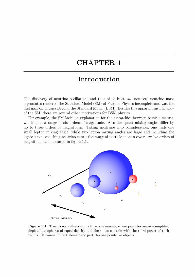
For example, the SM lacks an explanation for the hierarchies between particle masses,which span a range of six orders of magnitude. Also the quark mixing angles differ byup to three orders of magnitudes. Taking neutrinos into consideration, one finds onesmall lepton mixing angle, while two lepton mixing angles are large and including thelightest non-vanishing neutrino mass, the range of particle masses covers twelve orders ofmagnitude, as illustrated in figure 1.1.
Figure 1.1: True to scale illustration of particle masses, where particles are oversimplifieddepicted as spheres of equal density and their masses scale with the third power of theirradius. Of course, in fact elementary particles are point-like objects.

3
In the SM the particle masses and mixing angles are free parameters and the seesawmechanisms explaining small neutrino masses also have to fix the lepton mixing anglesby hand. The number of flavour related parameters and their striking hierarchies withinand between different families constitutes the so called flavour problem of Particle Physics.One attractive solution is the idea of flavour symmetries, which can unify particles ofdifferent families. When a flavour symmetry is spontaneously broken, predictions for theYukawa matrices emerge from vacuum expectation values (vevs) of dynamical fields and itis possible to explain the different flavour structures.
Another BSM concept towards a more fundamental theory of Elementary ParticlePhysics are Grand Unified Theories (GUTs). They unify the SM gauge group into a singlesimple gauge group at higher energies than those accessible to SM physics. And they unifySM fermions within a family into joint representations of the GUT gauge group. Thusthey can make predictions for relations between e.g. quark and lepton masses of the samegeneration, making GUTs an attractive framework to address the flavour problem.
Two challenges arise when the SM is embedded into GUTs. Firstly, the SM gaugecouplings do not unify and secondly too rapid proton decay mediated by heavy vectorbosons is predicted. Both are avoided with the introduction of Supersymmetry (SUSY).With a relatively low mass scale of sparticles, the gauge couplings successfully unify and themass of the additional vector bosons is high enough to suppress proton decay sufficiently.Additionally, low energy SUSY is a solution to the hierarchy problem by explaining anaturally low Electroweak scale and the lightest sparticle is a candidate for dark matter.
The focus of this thesis are SUSY flavour GUT models, which are BSM theories thatcombine the attractive ideas of SUSY, GUTs, and flavour symmetries. Particularly in-teresting subjects in SUSY flavour GUT models are the interdependencies between thevarious sectors of the models, as outlined in figure 1.2. Predictions obtained from the
GUTs SUSY
Flavour
SUSYFlavourGUTsQ
uark
–Lep
ton
rela
tion
s
proton decay
Sparticlem
asses
Figure 1.2: SUSY flavour GUT models feature an interplay between three “different”sectors of BSM physics.
(spontaneously broken) flavour symmetry are valid at the GUT scale. To test those pre-dictions at lower energies the Renormalisation Group Equations (RGEs) have to be solved.Since, when heavy degrees of freedom are integrated out, SUSY and GUT breaking effects

4 1. Introduction
play an important role in the precise solution of the RGEs, there is a variety of predictionsemerging from SUSY, GUTs, and flavour symmetries which influence each other.
The presentation of the author’s research is divided into three parts. In part III wefocus on the construction of predictive SUSY flavour GUT models with realistic quark-lepton mass ratios and mixing angles relations, sketched as the left edge in the triangleof figure 1.2. In chapter 6 we present four simple conditions for unified models to predictthe observed relation between the Cabibbo angle and the small 1-3 lepton mixing angle.These conditions are then realised in a SUSY flavour GUT model in chapter 7, where wecarefully construct additional discrete symmetries and a renormalisable messenger sectorto protect the model from dangerous effective operators. A second SUSY flavour GUTmodel, similar to the first but with an inverse neutrino mass ordering, is constructed inchapter 8. Both models are fitted to experimental data and we perform Markov ChainMonte Carlo analyses. Among others we predict the unmeasured neutrino CP phases anddiscuss how the models can be tested by future experiments.
Part IV discusses the problem of doublet-triplet splitting and the related question ofproton decay in SUSY SU(5), as shown as the lower edge of figure 1.2. We introduce asecond GUT breaking Higgs field in the adjoint representation, which allows the adjointsto carry charges under additional discrete symmetries. We present two example modelscombining the double missing partner mechanism with viable GUT scale predictions forthe quark-lepton Yukawa coupling ratios. We calculate the effective masses of the colourtriplets mediating proton decay and find that in both models proton decay is sufficientlysuppressed.
The final part V is focused on the important effects of SUSY threshold corrections onthe investigation of flavour GUT models. The size of these corrections depends on thedetails of the SUSY sector and the sparticle masses, which we illustrate on the right edgeof figure 1.2. We calculate the full one-loop SUSY threshold corrections to the MSSMYukawa coupling matrices and introduce a new software tool SusyTC as an extension tothe Mathematica package REAP. Finally we investigate the predictions of an example GUTmodel with realistic quark-lepton Yukawa coupling ratios for the CMSSM soft-breakingparameters and sparticle masses.
The appendices A and C contain brief reviews of group theory and Markov ChainMonte Carlo techniques used in this thesis, respectively. Appendices B, E, F, and Gcontain extensive formulae and equations used in chapter 10, as well as the documentationfor SusyTC. Appendix D contains additional information for the flavour models of thisthesis, such as details on additional symmetries and charges of the models’ fields and themessenger sectors.
In the next part II the theoretical framework for the main parts of this thesis are reviewedand our notations and conventions are introduced. Chapter 2 introduces the SM, chapter3 reviews massive neutrinos, in chapter 4 we discuss GUTs, and in chapter 5 SUSY isreviewed.

PART II
Theoretical Framework

CHAPTER 2
The Standard Model of Particle Physics
In the mid-20th century the effort to develop a thorough understanding of the variousphenomena of Elementary Particle Physics led to the construction of the Standard Model(SM) of Particle Physics [6–9]. To its great successes belong the correct predictions ofthe neutral current (the existence of the Z0 vector boson), the existence of the top quark,and the existence of a fundamental scalar boson as a result of the Brout-Englert-Higgsmechanism [10, 11], known as Higgs boson. Despite these major achievements, there aremany motivations suggesting the SM is incomplete and expected to be embedded into amore fundamental theory.
This chapter is devoted to an introduction to the SM, setting the background formalism,notation, and conventions necessary for the reminder of this thesis. Finally some of theopen questions in the SM are addressed, motivating physics Beyond the Standard Model(BSM) and the main part of this thesis.
2.1 Gauge interactions and field content
The SM is a chiral, renormalisable gauge quantum field theory with the gauge group givenby GSM = SU(3)C × SU(2)L × U(1)Y , a direct product of the gauge group of QuantumChromodynamics (QCD) SU(3)C , where the C refers to colour, and of the Electroweak(EW) theory SU(2)L × U(1)Y , with L for left and Y denoting hypercharge. Becauseof the local invariance under GSM, massless spin one fields emerge, which are identifiedwith the force carriers of the SM. These gauge bosons are named gluons (Ga
µ) for QCD,W aµ for SU(2)L and Bµ for U(1)Y . Since U(1)Y is an Abelian group, Bµ does not carry
hypercharge, whereas Gaµ and W a
µ transform in the adjoint representations of SU(3)C andSU(2)L, respectively.1
The matter fields of the SM are fermions with spin 12. They split into quarks, which
transform in the fundamental representation of SU(3)C , and leptons, which are coloursinglets. The left- and right-handed components of the SM fermions transform differently
1A brief review on group theory can be found in Appendix A.

2.1 Gauge interactions and field content 7
Gauge bosons
Gµ (8,1)0
Wµ (1,3)0
Bµ (1,1)0
Matter fields
Q1 =
(uLdL
)Q2 =
(cLsL
)Q3 =
(tLbL
)(3,2) 1
6
uR cR tR (3,1) 23
dR sR bR (3,1)− 13
L1 =
(νeLeL
)L2 =
(νµLµL
)L3 =
(ντLτL
)(1,2)− 1
2
eR µR τR (1,1)−1
Higgs field
φ (1,2) 12
Table 2.1: Field content of the SM with the corresponding GSM representations andhypercharge QY listed as (SU(3)C , SU(2)L)QY
under the SM gauge group: The left-handed fermions transform in the fundamental rep-resentation of SU(2)L, while the right-handed fermions are SU(2)L singlets. The matterfields are thus an SU(2)L doublet Q containing the left-handed quark fields uL and dL,an SU(2)L doublet L containing the left-handed electron and neutrino, eL and νL, re-spectively, the right-handed quark fields uR and dR, and a right-handed electron field eR.2
These particles appear in three copies, also called families, in nature, which have exactlyidentical couplings to the gauge bosons. The different quark and lepton species are denotedflavours.
Next to gauge bosons and fermions, the SM also contains a fundamental, complex spin0 field. This so called Higgs field is an SU(2)L doublet and plays a crucial role in theBrout-Englert-Higgs mechanism, described in the next section. All fields of the SM arelisted in table 2.1 together with their quantum numbers under GSM. Using natural units~ = c = 1 and a mostly minus convention for the Minkowksi metric
ηµν = diag(+1,−1,−1,−1) , (2.1)
the most general renormalisable Lagrange density with this field content is given by3:
LSM = −1
4GaµνG
µνa − g23θQCD64π2
εµνλρGλρaGµνa − 1
4WAµνW
µνA − 1
4BµνB
µν
2There are no right-handed neutrinos in the SM. We discuss the extension of the SM by right-handedneutrino fields in the next chapter.
3Note that we use the two-component Weyl spinor representation for the fermion fields. An extensivereview including conversion formulae to four-component representations can be found in [12].

8 2. The Standard Model of Particle Physics
+ iQ†i σµDµQi + iu†Riσ
µDµuRi + id†RiσµDµdRi
+ iL†i σµDµLi + ie†Riσ
µDµeRi
+ (Dµφ)†Dµφ− V (φ†φ)
− YuijQi · φu†Rj + YdijQi · φ d†Rj + YeijLi · φ e†Rj + h.c. , (2.2)
where implicitly sums over the SU(3)C , SU(2)L, and family indices a = 1 . . . 8, A = 1 . . . 3,and i = 1 . . . 3, respectively, are understood. Since the matter fields come in three familiesof equal quantum numbers, they can mix and the Yukawa couplings Yf of the fermions tothe Higgs field are in general complex 3× 3 matrices. The gauge field strengths are givenby
Gaµν ≡ ∂µG
aν − ∂νGa
µ − g3fabcG
bµG
cν , (2.3)
WAµν ≡ ∂µW
Aν − ∂νWA
µ − g2εABCWBµ W
Cν , (2.4)
Bµν ≡ ∂µBν − ∂νBµ , (2.5)
where g3 and g2 are the gauge coupling strengths and fabc and εABC the structure constantsof the gauge groups SU(3)C and SU(2)L, respectively, as discussed in appendix A. Thegauge covariant derivative of a field ψ is defined as
Dµψ ≡(∂µ − ig3G
aµT
a − ig2WAµ τ
A − ig′BµQY
)ψ , (2.6)
where g′ is the gauge coupling strength of U(1)Y , T a and τA are the generators of theSU(3)C and SU(2)L representations of ψ, and QY denotes the hypercharge of ψ. V (φ†φ)is the scalar potential of the Higgs field (2.13). Finally we used
σµ ≡ (1,−~σ) , (2.7)
χ · ξ ≡ εABχAξB , (2.8)
φ ≡ εφ∗ , (2.9)
with σi denoting the Pauli matrices
σ1 =
(0 11 0
), σ2 =
(0 −ii 0
), σ3 =
(1 00 −1
), (2.10)
and the totally antisymmetric tensors εAB of SU(2)L and εµνλρ with
ε12 = −ε21 = 1 and ε0123 = −ε0123 = 1 . (2.11)
2.2 The Brout-Englert-Higgs mechanism
Since W± and Z0 bosons are found to be massive vector bosons in nature, the SM needsto contain a mechanism in order to explain gauge boson masses in the EW sector. The

2.2 The Brout-Englert-Higgs mechanism 9
Stuckelberg formalism [13] could in principle generate massive gauge bosons, the resultingtheory would be non-renormalisable, however. An elegant solution that keeps the theoryrenormalisable is the incorporation of the Brout-Englert-Higgs (BEH) mechanism [10, 11]into the SM, by which massive W± and Z0 emerge from the spontaneous symmetry break-ing of SU(2)L × U(1)Y → U(1)em:
The scalar potential of the complex Higgs field
φ =
(φ+
φ0
)(2.12)
is given byV (φ†φ) = µ2φ†φ+ λ(φ†φ)2 . (2.13)
The BEH mechanism assumes µ2 < 0 and thus the minimum of the Higgs potential doesnot coincide with vanishing field value of φ. Rather, the Higgs field obtains a non-vanishingvacuum expectation value (vev)
〈φ〉 =1√2
(0v
). (2.14)
This ground state is not invariant under SU(2)L × U(1)Y , but it respects an U(1)em sym-metry, which is identified with the gauge group of electromagnetism. The electric chargeis given by
Qe = τ 3 +QY . (2.15)
Expanding φ around its vev one can perform a gauge transformation, such that threedegrees of freedom are absorbed by the gauge fields, which get mass terms in doing so,while one real massive scalar, the Higgs boson h, remains in the particle spectrum. Thenew gauge bosons are linear combination of the gauge bosons in the unbroken theory. Theyare given by
W±µ =
1√2
(W 1µ ∓W 2
µ
), (2.16)(
Z0µ
Aµ
)=
(cos θW − sin θWsin θW cos θW
)(W 3µ
Bµ
), (2.17)
where Aµ is the massless photon field and the weak mixing angle θW is defined by
sin2 θW =g′2
g22 + g′2
= 0.23155(5) [14] . (2.18)
The masses of the gauge bosons are given in terms of gauge couplings and the vev as
MW± =1
2g2v and MZ0 =
1
2
√g2
2 + g′2 v . (2.19)
Experimentally the masses of the weak gauge bosons are known to be [14]
MW± = (80.385± 0.015) GeV and MZ0 = (91.1876± 0.0021) GeV . (2.20)

10 2. The Standard Model of Particle Physics
The value of v ≈ 246 GeV can be obtained from these measurements. Finally, the mass ofthe Higgs boson was found to be [14]
mh = (125.7± 0.4) GeV . (2.21)
2.3 Fermion masses and the Cabibbo-Kobayashi-Maskawa-
Matrix
Besides the breaking of electroweak symmetry, the non-vanishing vev of the Higgs fieldalso leads to the appearance of fermion mass matrices
Muij =v√2Yuij , Mdij =
v√2Ydij , and Meij =
v√2Yeij . (2.22)
The 3× 3 mass matrices Mf can be diagonalised by a singular value decomposition (SVD)(U
(f)L
)TMf
(U
(f)R
)∗= diag
(m
(f)1 , m
(f)2 , m
(f)3
), (2.23)
where U(f)L and U
(f)R are unitary 3 × 3 matrices4 and m
(f)i are the three singular values
of Mf . In the SM six unitary matrices are introduced to rotate the quarks and chargedleptons from the flavour basis to the mass basis
uL → U(u)L uL , dL → U
(d)L dL , eL → U
(e)L eL ,
uR → U(u)R uR , dR → U
(d)R dR , eR → U
(e)R eR . (2.24)
Neutrinos are massless in the SM, therefore in the transformation to the mass basis theneutrino fields are rotated in correspondence with the charged lepton field
νL → U(e)L νL . (2.25)
With the exception of the couplings to the charged gauge bosons W±µ , all interaction
terms in the SM are flavour diagonal and are thus left invariant by the transformation of(2.24). For the coupling to W±
µ , however, the transformation to the mass basis leads tothe emergence of the unitary Cabibbo-Kobayashi-Maskawa (CKM)-Matrix [15,16]
VCKM ≡(U
(u)L
)†U
(d)L (2.26)
in the interaction Lagrange density of the charged current
Lcc =g2√
2
(u†LVCKMσ
µW+µ dL + ν†σµW+
µ eL
)+ h.c. . (2.27)
4Note that the matrices U(f)L and U
(f)R are not uniquely determined by (2.23), since the matrices(
U(f)L diag(eiγ1 , eiγ2 , eiγ3)
)Tand
(U
(f)R diag(eiγ1 , eiγ2 , eiγ3)
)∗also diagonalise Mf .

2.3 Fermion masses and the CKM-Matrix 11
A 3× 3 unitary matrix has in general nine real parameters, whereas a 3× 3 orthogonalmatrix has three real parameters. The additional six real parameters in the unitary casecan therefore be identified as complex phases. One can thus parametrise a general 3 × 3unitary matrix by [17]
V = U23U13U12P , (2.28)
with
U23 =
1 0 00 c23 s23e−iδ23
0 −s23eiδ23 c23
, U13 =
c13 0 s13e−iδ13
0 1 0−s13eiδ13 0 c13
,
U12 =
c12 s12e−iδ12 0−s12eiδ12 c12 0
0 0 1
, and P =
eiγ1 0 00 eiγ2 00 0 eiγ3
, (2.29)
where sij and cij denote sin θij and cos θij, respectively. For the CKM matrix
VCKM = UCKM23 UCKM
13 UCKM12 PCKM (2.30)
the mixing angle θCKM12 is given a special name and is referred to as Cabibbo angle θC .
Taking advantage of the freedom in the SVD to multiply the unitary matrices U(u)L and
U(d)L by diagonal phase matrices, complex phases of VCKM can be absorbed in the phases
of the quark fields. Although there are six quark fields at hand, because the full SMLagrangian is invariant under a global rotation of all quarks by a common phase, only fivecomplex phases of VCKM can be absorbed. With the new unitary matrices
U(u)L → U
(u)L diag
(1, eiδCKM
12 , ei(δCKM12 +δCKM
23 ))
and U(d)L → U
(d)L
(PCKM
)−1diag
(1, eiδCKM
12 , ei(δCKM12 +δCKM
23 ))
(2.31)
the CKM matrix is brought into the Particle Data Group (PDG) standard parametrisation[14]
VCKM =
c12c13 s12c13 s13e−iδ
−c23s12 − s23s13c12eiδ c23c12 − s23s13s12eiδ s23c13
s23s12 − c23s13c12eiδ −s23c12 − c23s13s12eiδ c23c13
, (2.32)
where for the sake of readability the superscript CKM has been dropped on all parameters.The CP violating phase δCKM is given in terms of [17]
δCKM = δCKM13 − δCKM
12 − δCKM23 . (2.33)
The experimental values reported by the PDG are given as [14]
θCKM12 = 13.02 ± 0.036 , θCKM
13 = 0.204 ± 0.0099 ,
θCKM23 = 2.37 ± 0.071 , δCKM = 71.7 ± 3.1 . (2.34)

12 2. The Standard Model of Particle Physics
Finally, the masses of the fermions are reported. The masses of the electron and muonare most precisely determined from atomic physics experiments, causing the uncertaintyof the precise value of the atomic mass unit u in MeV to be the dominant contribution tothe mass uncertainty of me and mµ [18]
me = (0.510998928± 0.000000011) MeV ,
mµ = (105.6583715± 0.0000035) MeV . (2.35)
The mass of the tau lepton is obtained from experiments measuring the production crosssection e−e+ → τ−τ+ [14]
mτ = (1776.82± 0.16) MeV . (2.36)
Free quarks are not observed in nature, rendering the quark mass determination a verydifficult endeavour. Due to the absence of a physical observable, quark masses have to bereported in a mass independent renormalisation scheme, such as MS at a certain renor-malisation scale. The masses of the light quarks u, d, and s are determined from latticeQCD [19] and chiral perturbation theory [20,21]. The PDG reports the light quark masses
in MS at a renormalisation scale µ = 2 GeV [14]
mu = 2.3+0.7−0.5 MeV , md = 4.8+0.5
−0.3 MeV , ms = (95± 5) MeV . (2.37)
Note that chiral perturbation theory determines quark mass ratios rather than absolutequantities and needs additional input from e.g. lattice theory to obtain specific quarkmasses. Therefore often the reported light quark mass ratios5 are used
ms
md
= 18.9± 0.8 [22] andms
12
(mu +md)= 27.5± 1.0 [14]. (2.38)
The masses of the heavy quarks are obtained from measured qq production cross sectionsand in the case of bottom and charm, lattice simulations and heavy quark effective theory[23] of the D and B mesons. For b and c the heavy quark masses are given as MS mass ata renormalisation scale equal to their respective quark mass [14]
mc(mc) = (1.275± 0.025) GeV ,
mb(mb) = (4.18± 0.03) GeV . (2.39)
Because of its very heavy mass the top quark has the unique feature among all quarks todecay before it can form tt bound states, allowing to determine its pole mass [14]
mt = (173.21± 0.51± 0.71) GeV , (2.40)
in analogy with the determination of the τ pole mass.
5In pure QCD these mass ratios are independent from the renormalisation scale in the MS scheme andare therefore reported at µ = 2 GeV. In the full SM they are scale dependent, however.

2.4 Open questions in the Standard Model 13
Aρc
Aµa
Aνb
Figure 2.1: Triangle diagram with chiral fermions in the loop and three external gaugebosons, possibly leading to an anomaly. In general the gauge bosons need not to be of thesame gauge group.
2.4 Open questions in the Standard Model
We close this chapter with a brief discussion of various open problems and deficiencies ofthe Standard Model. The following chapters will bring widely expected solutions to theseopen problems into focus and introduce several Beyond the Standard Model extension ofParticle Physics. The last concern in the following list motivates the main parts of thisthesis.
Neutrino masses The SM predicts vanishing masses of neutrinos. This is in contra-diction with the observation of neutrino oscillations and therefore the strongest indicationthat BSM physics is needed to understand the phenomena of Particle Physics. Chapter 3is devoted to massive neutrinos and neutrino mixing.
U(1)em Charge quantisation For the SU(3)C and SU(2)L subgroups of the SM gaugegroup, the interaction between gauge bosons and fermions is defined purely by group theoryand the gauge coupling strengths g3 and g2. This guarantees universality, e.g. all SU(2)Ldoublets couple the same way to the gauge bosons W a
µ . In contrast, there is no such mech-anism guaranteeing U(1)Y hypercharge universality. Within the SM there is no theoreticalreason, but solely experimental observation, that QY is quantised and distributed to theSM matter fields as listed in table 2.1. Chapter 4 discusses Grand Unified Theories (GUTs),where the U(1)Y emerges from spontaneous breaking of a more fundamental gauge group.The group theoretical universal coupling of the more fundamental gauge group is theninherited by the SM U(1)Y , leading finally to U(1)em charge quantisation.
Anomaly cancellation Anomalies appear in chiral gauge theories, when a symmetryof the Lagrangian is not conserved by higher order loop terms [24, 25]. Triangle diagramswith three external gauge bosons as depicted in figure 2.1 can contribute to the anomaly ofa symmetry. In order for the gauge theory to stay anomaly free, the anomaly coefficients
Aabc ≡ Tr(T aT b, T c
)(2.41)

14 2. The Standard Model of Particle Physics
need to vanish [26], where T a, T b, and T c denote generators of the respective gauge group.Looking closer at one example with one external U(1)Y gauge boson and two externalSU(2)L gauge bosons, (2.41) reduces to the trace over the hypercharges
AY bc =δbc
2Tr QY =
3δbc
2
(3 ·(
1
6+
2
3− 1
3
)− 1
2− 1
)= 0 . (2.42)
As in (2.42) all other anomaly coefficients in the SM vanish. The crucial point is the can-cellation of lepton and quark contributions. Similar to the open question of U(1)Y chargequantisation, there is no theoretical reason for the leptons and quarks to carry preciselythe right hypercharges for the anomaly coefficients to vanish and thereby rendering theSM anomaly free. In GUTs leptons and quarks are unified in joint representations of theGUT gauge group, which in certain cases guarantees anomaly cancellation automatically.
Naturalness problem I - The hierarchy problem As the only scalar field in the SM,the Higgs boson is subject to much larger radiative corrections than the SM fermion fields.Whereas the radiative corrections to fermion masses are logarithmically divergent
δmf ∼ m0 log
(Λ2
m20
), (2.43)
the corresponding radiative corrections to the Higgs boson mass due to a fermion loop isquadratically divergent
δm2h ∼ |yf |2Λ2 , (2.44)
where we used a momentum cutoff regularisation of the divergent loop corrections.Since the Higgs mass is known to be around 126 GeV, an enormous amount of fine tuning
between the bare mass parameter and the counterterm has to appear in the renormalisation,otherwise the Higgs mass would be expected to be at a much higher energy scale associatedwith new physics, e.g. the Planck scale. Another way to view the unaturalness of smallmh is due to the fact that δm2
h is independent of m2h itself. Setting mh = 0 does therefore
not restore a symmetry of the Lagrange density and the smallness of mh fails to satisfyt’Hooft’s naturalness criterion [27]. Chapter 5 discusses Supersymmetry (SUSY), whichintroduces a bosonic partner to each fermion. Including the bosonic partner in the radiativecorrections, the quadratic divergence of mh vanishes to all order in perturbation theory.Additionally, some discrepancy between predictions of GUTs and phenomenology can beresolved when supersymmetric GUTs are studied.
The flavour problem There are in total nineteen parameters in the Standard ModelLagrange density (2.2) when using the freedom to absorb some phases of the CKM Matrixinto the quark fields as discussed in 2.3. The majority of those, thirteen parameters, belongto the flavour sector of the SM, parametrising nine fermion masses, three mixing anglesand the CKM phase. Including extensions of the SM to incorporate massive neutrinos,
2.4 Open questions in the Standard Model 15
as discussed in chapter 3, into the parameter counting, the number of flavour relatedparameters is even increased. As was shown in figure 1.1, looking at the values of theparticles’ masses, one encounters huge hierarchies, within single families, but also whencomparing the masses of different families. The CKM mixing angles are small, but it willbe seen in the next chapter, that some of the neutrino mixing angles are very large. The SMlacks an explanation of these patterns and hierarchies, and includes all flavour parametersfixed simply as measured from experiments. Expecting a more elegant explanation froma fundamental theory, one can build flavour models with discrete symmetries to describerelations among the measured flavour observables. In part III of this thesis, two suchflavour models are constructed within the framework of supersymmetry and GUTs, andtheir predictions are discussed in detail.
At the end of this chapter three open problems of the Standard Model are listed, thatlie outside the scope of this thesis. For the sake of completeness they are presented herenevertheless.
Naturalness problem II - The strong CP problem Although being a total deriva-tive, the CP violating θQCD term in the SM Lagrange density can not be dismissed dueto instanton effects [28]. When the quark mass matrices are diagonalised, due to a chiralanomaly the value of θQCD is changed [29]
θ = θQCD + Arg Det (MuMd) . (2.45)
Although one could expect θ to be of order O(1), from measurements of the neutron electricdipole moment it is known [14]
|θ| < 10−10 . (2.46)
The strong CP problem is the question for an explanation of small θ. One possible solutionis to extend the SM by a spontaneously broken U(1)PQ Peccei-Quinn symmetry [30] andeffectively replaces θ by the pseudo-Nambu-Goldstone boson of U(1)PQ, the axion [31].Another possible solution is spontaneous breaking of CP symmetry, such that θQCD = 0in the QCD sector, whereas Arg Det (MuMd) = 0 is enforced by flavour models [32].
Dark Matter Observations of rotation curves of galaxies [33], anisotropies in the CosmicMicrowave Background (CMB) [34, 35], and gravitational lensing of the bullet cluster [36]signalise the existence of Dark Matter (DM). Due to gravitational lensing surveys it isknown that the majority of DM has to be composed out of non-baryonic matter [37], thusa BSM explanation is required. Possible DM candidates are heavy sterile neutrinos, axions,and the lightest supersymmetric particle in SUSY [38–40].
Naturalness problem III - The cosmological constant problem From the ParticlePhysics point of view, it is always possible to add a constant term into the SM Lagrangedensity, without altering any prediction of the theory. Such a term corresponds to the

16 2. The Standard Model of Particle Physics
energy of the vacuum and it does become important in cosmology, where it is known ascosmological constant ρcc or dark energy to explain the observed accelerating expansion ofthe universe [41]. The value of the cosmological constant is [14]
ρcc ≈ (2.2 meV)4 . (2.47)
The SM is incapable of explaining any value of ρcc, but even when attempting an analysison dimensional grounds one expects contributions from quantum loop effects
ρ ∼ m4 , (2.48)
which could be cancelled by new physics at scales larger than at least TeV, leading to anestimate of ρcc that is at least 60 orders of magnitude larger than observed. So far, nosatisfying solution to the cosmological constant problem has been proposed and it remainsan open question.

CHAPTER 3
Massive neutrinos
In the process of developing the Standard Model of Particle Physics, it was assumed thatneutrinos are massless particles. In fact, the SM only contains left-handed neutrino fields,included in the SU(2)L doublets Li. With the observation of neutrino oscillations [42–46],the presumption of massless neutrinos has been falsified and one is compelled to extend theSM to account for very small neutrino masses. Excitingly, there are still open questionsand unmeasured observables in Neutrino Physics, such that no definite neutrino massgeneration mechanism exists.
This chapter introduces lepton mixing as general consequence of massive neutrinos anddiscusses some of the suggested SM extensions for neutrino masses. Finally a first briefintroduction towards flavour model building is presented. The content of this chapter isbased on [47–49].
3.1 Neutrino masses and the seesaw mechanisms
Besides observations of neutrino oscillations there is no evidence for neutrino masses fromother types of experiments. Measurements of β-decay set only an upper bound for themass of the electron-type anti-neutrino [50]
mνe < 2.05 eV . (3.1)
Anisotropies in the CMB and large-scale clustering of galaxies constrain the energy densityof neutrinos Ων and lead to an upper bound for the sum of light neutrino masses [35]∑
ν
mν < 0.23 eV . (3.2)
These masses are substantially smaller than the masses of quarks and charged leptons, thusthe flavour problem described in 2.4 got more severe with the discovery of non-vanishingneutrino masses.
There are two straightforward options for incorporating neutrino masses into the SM.One is to simply extend the particle content of the SM by right-handed neutrino fields νRi ,

18 3. Massive neutrinos
which transform as total singlets under the gauge group of the SM. Then the Lagrangedensity is extended by a new Yukawa coupling
Lν = iν†Riσµ∂µνRi −
(YνijLi · φ ν†Rj + h.c.
), (3.3)
which generates a Dirac mass when the Higgs field φ obtains its vev (2.14), just as quark andcharged lepton masses emerge when the electroweak symmetry gets broken. The numberN of right-handed neutrinos is left undetermined and Yν can be any general complex 3×Nmatrix. Since this option requires Yukawa coupling of O(10−12) to explain O(eV) neutrinomasses, the problem of naturalness remains unsolved.
Because the νRi are gauge singlets, additionally to (3.3) the Lagrange density can includea Majorana mass term
L = Lν −1
2MνijνRiνRj + h.c. , (3.4)
when one dismisses the Lepton number conservation of the original SM.The second straightforward suggestion to generate massive neutrinos results from the
abandonment of renormalisability of the SM. Then the SM is extended by the effectivedimension five Weinberg operator [51]
Lκ =1
2κij (Li · φ) (Lj · φ) + h.c. , (3.5)
which gives rise to a Majorana mass term
Lν =v2
4κijνLiνLj + h.c. (3.6)
after EW symmetry is broken.Particle Physics knows the non-renormalisable four-fermion Fermi theory of beta-decay,
which emerges from the renormalisable SM as effective theory when the heavy W± bosonare integrated out. Repeating this successful idea for non-renormalisable neutrino operatorsgives rise to the seesaw mechanisms: The Weinberg operator (3.5) is obtained as effectiveoperator by integrating out heavy degrees of freedom. With the resulting neutrino massesbeing inverse proportional to the mass of the heavy fields, the seesaw mechanism areattractive solutions to explain the smallness of neutrino masses without the necessity ofunnatural small couplings.
There are three different types of seesaw mechanisms, depending on what type of heavydegrees of freedom are introduced in order to generate (3.5). In this thesis we will exclu-sively make use of type-I seesaw [52], which is based on new heavy right-handed neutrinofields νRi and the SM Lagrange density is extended as in (3.4). When the heavy right-handed neutrinos are integrated out, the Weinberg operator emerges effectively and theneutrino Majorana mass is given by
mν = −v2
2YνM
−1ν Y T
ν , (3.7)

3.2 The PMNS-Matrix 19
when the SM Higgs field φ obtains its vev. Type-I seesaw is an attractive extension ofthe SM, since the gauge-singlets νRi can naturally have large Majorana masses, leading toan explanation of the smallness of neutrino masses. When the SM is embedded into anSO(10) GUT, a right-handed neutrino νRi is automatically included in the spectrum, aswill be discussed in the next chapter.
Other seesaw mechanism are obtained from heavy scalar SU(2)L triplets (type-II [53])or from fermion SU(2)L triplets (type-III [54]). Another mechanism for neutrino massgeneration is the double seesaw mechanism [55], where the right-handed neutrinos of theseesaw type-I are originally massless and the heavy mass Mν is itself an effective massoriginating from another instance of the seesaw mechanism with sterile neutrinos νSi , whichdo not couple to the SM doublets Li. Finally there is the possibility to explain smallneutrino masses as loop corrections to vanishing tree-level masses [56], but such models doalso need new particles in addition to the SM particles to run inside the loop and can bemade arbitrarily complex.
3.2 The Pontecorvo-Maki-Nakagawa-Sakata
Matrix
In the SM the neutrinos were assumed to be massless and rotated like the charged leptons(2.25) when transforming from the flavour basis to the mass basis. Massive neutrinos,however, require to diagonalise the neutrino mass matrix as well. If neutrinos have a Diracmass, the mass matrix can be diagonalised by a singular value decomposition as for thequarks and charged leptons (2.23). For Majorana neutrinos, however, mν is a complexsymmetric matrix, and therefore has to be diagonalised by a Takagi decomposition (TD)
UT(ν)mνU(ν) = diag (m1,m2,m3) , (3.8)
where U(ν) is an unitary 3× 3 matrix and mi are the three singular values of the complexsymmetric matrix mν . As for SVD, U(ν) is not uniquely defined by (3.8). In SVD theunitary matrices are defined up to a diagonal phase matrix, which in TD is in generalreduced to a sign ambiguity
U(ν) → U(ν) diag(eiγ1 , eiγ2 , eiγ3
), (3.9)
with γi = 0, π. Only if the corresponding singular value mi is vanishing, γi can be arbitrary.With (2.24) the rotations to the mass basis in the lepton sector are
eL → U(e)L eL , eR → U
(e)R eR , and νL → U(ν)νL . (3.10)
The coupling of leptons to the neutral current is flavour diagonal as for quarks. In thecoupling to the charged current the transformations (3.10) lead to the emergence of theunitary Pontecorvo-Maki-Nakagawa-Sakata (PMNS)-Matrix [42, 57]
VPMNS ≡(U
(e)L
)†U(ν) (3.11)

20 3. Massive neutrinos
inLcc =
g2√2
(u†LVCKMσ
µW+µ dL + e†LVPMNSσ
µW−µ νL
)+ h.c. . (3.12)
As for the CKM-Matrix (2.3), at first the PMNS-Matrix can be parametrised in terms of(2.29) with three real angles and six phases as
VPMNS = UPMNS23 UPMNS
13 UPMNS12 PPMNS . (3.13)
Three phases can be absorbed in the charged lepton fields using the freedom of U(e)L as
U(e)L → U
(e)L diag
(eiγPMNS
1 , ei(γPMNS1 +δPMNS
12 ), ei(γPMNS1 +δPMNS
12 +δPMNS23 )
). (3.14)
This brings VPMNS into its standard parametrisation
VPMNS =
c12c13 s12c13 s13e−iδ
−c23s12 − s23s13c12eiδ c23c12 − s23s13s12eiδ s23c13
s23s12 − c23s13c12eiδ −s23c12 − c23s13s12eiδ c23c13
Pα , (3.15)
where for readability the superscript PMNS has been dropped. Pα is a diagonal phasematrix containing the two Majorana phases α1 and α2
Pα = diag
(1, ei
αPMNS1
2 , eiαPMNS
22
). (3.16)
The three physical phases of VPMNS are given in terms of the parametrisation (3.13) as1
δPMNS = δPMNS13 − δPMNS
12 − δPMNS23 , (3.17a)
αPMNS1
2= γPMNS
2 − γPMNS1 − δPMNS
12 , (3.17b)
αPMNS2
2= γPMNS
3 − γPMNS1 − δPMNS
12 − δPMNS23 . (3.17c)
In the case that neutrinos are Dirac particles, mν is diagonalised by a SVD and the PMNS-Matrix is analogously to the CKM-Matrix obtained, i.e. the Majorana phases are unphys-ical.
Neutrino oscillations arise due to the fact that neutrinos are created and observed viacharged current interactions as flavour eigenstates |να〉, which are superpositions of masseigenstates2 |νi〉
|να〉 = U∗αi|νi〉 . (3.18)
1In the literature one also finds the convention of Pα = diag(
e−iφ12 , e−i
φ22 , 1
), in which case the
Majorana phases are given asφPMNS1
2 = γPMNS3 − γPMNS
1 − δPMNS12 − δPMNS
23 andφPMNS2
2 = γPMNS3 − γPMNS
2 −δPMNS23 , respectively, whereas the Dirac phase is unchanged from (3.17a).
2Note that in contrast to the field rotation in (3.10) the complex conjugate U∗αi appears in the trans-formation of states, because in standard convention of quantum field theory a quantum field contains thecreation operator for an anti-particle state |ψ〉 = ψ|0〉.

3.2 The PMNS-Matrix 21
If one is interested in oscillations of the three active light neutrinos of the SM, U is identifiedwith VPMNS. More generally however, U can also describe oscillations into sterile neutrinos.
The different mass eigenstates in a neutrino beam evolve differently and the probabilityof detecting a specific neutrino flavour eigenstate is thus time-dependent. Since neutrinosare ultra relativistic particles, the time-dependence is exchanged for a dependence on thedistance L between the places of origin and detection. Due to weak current interactions ofνe with electrons in matter, oscillations of νe also depend on the electron density ne [58].
In vacuum the probability for a flavour eigenstate |να〉 to oscillate into |νβ〉 is givenby [43,59,60]
P (να → νβ) =∑i
|Uαi |2|Uβi|2 +∑i>j
U∗αiUβiUαjU∗βje−i
∆m2ijL
2E , (3.19)
which is independent of the Majorana phases. This probability furthermore does notdepend on the absolute neutrino masses, but rather depends on the differences of thesquared masses
∆m2ij = m2
i −m2j . (3.20)
Thus it is impossible to inquire an overall scale of neutrino masses from vacuum neutrinooscillation experiments. If ∣∣∆m2
ijL∣∣ 4πE , (3.21)
the oscillation due to ∆m2ij are negligible, since the distance between neutrino source and
detection is much smaller than the oscillation length
Loscij ≡4πE∣∣∆m2
ij
∣∣ . (3.22)
When the uncertainty of the size ∆L or energy ∆E for neutrino production or detectionare much larger than Loscij , the neutrino oscillations due to ∆m2
ij get averaged [61].In the case of three oscillating neutrinos, conventionally one labels the neutrino mass
states such that
0 < ∆m221 , ∆m2
21 < |∆m232| , ∆m2
21 < |∆m231| . (3.23)
Then there are two options for the remaining neutrino mass m3, denoted as normal ordering(NO) and inverse ordering (IO), respectively
m1 < m2 < m3 (NO) ,
m3 < m1 < m2 (IO) . (3.24)
Experiments have not yet succeeded to distinguish between these mass orderings. A globalfit of neutrino oscillation measurements finds [62]
∆m221 = 7.50+0.19
−0.17 · 10−5 eV2 ,
∆m231 (N0) = +2.457+0.047
−0.047 · 10−3 eV2 ,
∆m232 (I0) = −2.449+0.048
−0.047 · 10−3 eV2 . (3.25)
22 3. Massive neutrinos
Because of ∆m221 |∆m2
31(32)| and distinct neutrino energies for specific oscillation exper-iments, one can find separate regimes of experiments, where a single mass squared split-ting dominates. The observed solar νe → νµ,τ oscillations are related to ∆m2
21, whereasthe larger of the two mass squared splittings ∆m2
31 and ∆m232, is related to atmospheric
νµ → ντ oscillations. Therefore one often refers to these mass splittings as
∆m2sol = ∆m2
21 , ∆m2atm =
∆m2
31 (NO)
∆m232 (IO)
. (3.26)
The experimental values of the lepton mixing angles are given by [62]
θPMNS12 = 33.48 +0.78
−0.75 and θPMNS13 = 8.50 +0.20
−0.21 . (3.27)
The global best-fit value of θPMNS23 depends on whether a normal or an inverse mass ordering
is assumed as prior
θPMNS23 =
42.3 +3.0
−1.6 (NO)
49.5 +1.5
−2.2 (IO). (3.28)
With small θPMNS13 , solar and atmospheric neutrino oscillations can be understood to be
dominantly two-flavour oscillations, where θPMNS12 is identified as solar mixing angle θsol and
atmospheric neutrino oscillations are related to the atmospheric mixing angle θatm ≡ θPMNS23 .
Oscillation experiments measuring the survival rate of νe from nuclear reactors are mostsensitive to corrections due to non-vanishing θPMNS
13 , which is therefore sometimes referredto as reactor mixing angle.
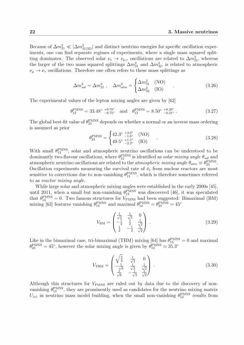
While large solar and atmospheric mixing angles were established in the early 2000s [45],until 2011, when a small but non-vanishing θPMNS
13 was discovered [46], it was speculatedthat θPMNS
13 = 0. Two famous structures for VPMNS had been suggested: Bimaximal (BM)mixing [63] features vanishing θPMNS
13 and maximal θPMNS12 = θPMNS
23 = 45
VBM =
1√2
1√2
0
−12
12
1√2
12−1
21√2
. (3.29)
Like in the bimaximal case, tri-bimaximal (TBM) mixing [64] has θPMNS13 = 0 and maximal
θPMNS23 = 45, however the solar mixing angle is given by θPMNS
12 ' 35.3
VTBM =
√
23
1√3
0
− 1√6
1√3
1√2
1√6− 1√
31√2
. (3.30)
Although this structures for VPMNS are ruled out by data due to the discovery of non-vanishing θPMNS
13 , they are prominently used as candidates for the neutrino mixing matrixU(ν) in neutrino mass model building, when the small non-vanishing θPMNS
13 results from

3.2 The PMNS-Matrix 23
(U
(e)L
)†, as so-called charged lepton correction to the neutrino mixing angle θν13 = 0. As-
suming “small” charged lepton mixing angles and θν13, respectively, one can perform a smallangle expansion of (3.11) to find [65]
sPMNS23 e−iδ
PMNS23 ≈ sν23e
−iδν23 − θe23c
ν23e−iδe
23 , (3.31a)
θPMNS13 e−iδ
PMNS13 ≈ θν13e
−iδν13 − θe13c
ν23e−iδe
13 − θe12e−iδe
12(sν23e−iδν23 − θe
23cν23e−iδe
23) , (3.31b)
sPMNS12 e−iδ
PMNS12 ≈ sν12e
−iδν12 + θe13c
ν12s
ν23e
i(δν23−δe13) − θe
12cν23c
ν12e−iδe
12 , (3.31c)
in leading order of θν13. The higher order term proportional to θe12θ
e23 is shown in (3.31b),
since it demonstrates that (3.31b) can be rewritten as
θPMNS13 e−iδ
PMNS13 ≈ θν13e
−iδν13 − θe13c
ν23e−iδe
13 − θe12s
PMNS23 e−i(δ
e12+δPMNS
23 ) . (3.32)
An especially interesting case is when θν13 and θe13 vanish, and one can derive from (3.32)
the interesting relationθPMNS
13 ≈ θe12s
PMNS23 , (3.33)
highlighting that θPMNS13 can result purely from charged lepton corrections. If one further-
more assumes θe23 θe
12, one obtains from (3.31), using (3.17a), the lepton mixing sumrule [65–67]
sν12 ≈ sPMNS12 − θPMNS
13 cPMNS12 cot θPMNS
23 cos δPMNS , (3.34)
to leading order in θPMNS13 . (3.33) and (3.34) will be in the center of the discussion in
chapter 6 and motivate much of the work in part III.We now turn to a discussion of the phases in VPMNS. It was already mentioned that
the neutrino oscillation probability (3.19) does not depend on the Majorana phases. Inneutrino oscillations, CP violation can be parametrised by the Jarlskog invariant J definedby [68]
Im(U∗αiUβiUαjU
∗βj
)≡ J
∑k,γ
εαβγεijk , (3.35)
which is independent of the phase convention for U . Note that CP violation can only beobserved in flavour violating oscillation measurements να 6= νβ. For oscillations of threelight neutrinos U = VPMNS one obtains
J = c213s13c12s12c23s23 sin δ , (3.36)
where again the superscripts PMNS have been dropped for readability. It follows thatCP violation is only observable in vacuum neutrino oscillations if all lepton mixing anglesare non-vanishing. Therefore only the recent detection of non-vanishing θPMNS
13 opened thepossibility to discover CP violation in neutrino oscillation experiments. Today global fitsreport hints towards a value of [62]
δPMNS =
306 +39
−70 (NO)
254 +63
−62 (IO). (3.37)

24 3. Massive neutrinos
For the studies and numerical fits in this thesis, the value of δPMNS has been kept anopen parameter, however. A future measurement of δPMNS can be expected from the longbaseline neutrino oscillation experiment DUNE [69], which will also be able to measure thesign of ∆m2
31 and determine the neutrino mass ordering.We conclude this section with a brief discussion of the Majorana phases αPMNS
1 andαPMNS
2 . In comparison to a Dirac mass matrix, which can be diagonalised by a SVD, aMajorana mass matrix has to be diagonalised by a TD, and therefore the Majorana phasesare physical and can not be absorbed by neutrino fields. Whether neutrino mass is ofDirac or Majorana type, can be distinguished by neutrinoless double beta decay (2β0ν) [70]:In such processes two nucleons simultaneously experience beta decay. If neutrinos havea Majorana mass, instead of two antineutrinos and two charged leptons with continousspectrum, the antineutrino emitted by one W boson can be absorbed as neutrino by thesecond W , leading to a final state of 2β0ν with two monochromatic charged leptons. Therate of this process is proportional to the effective Majorana mass
〈mββ〉 =
∣∣∣∣∣∑i
U2eimi
∣∣∣∣∣ = c212c
213m1 + s2
12c213e
iα1m2 + s213e
i(α2−2δ)m3 , (3.38)
where the superscript PMNS was dropped for readability. Because the mixing angles andmass squared splittings are known from oscillation experiments, a measurement of 〈mββ〉could, additionally to answering the Majorana or Dirac mass question, bring insights intoCP violation due to Majorana phases and into the question of whether neutrino massesfollow normal mass ordering, inverse mass ordering, or are nearly degenerate.3 A carefulaverage of various 2β0ν experiments leads to a conservative upper bound [72]
〈mββ〉 < 0.46 eV . (3.39)
3.3 Neutrino mass models & flavour model building
We close this chapter with a discussion of neutrino mass models, whose aim is to explainsimple structures of VPMNS, such as tri-bimaximal mixing, from discrete symmetries. Ina basis where the charged lepton Yukawa coupling matrix is diagonal one can phrase theneutrino mass matrix mν from (3.8) as [73]
mν = V ∗PMNS diag (m1,m2,m3)V †PMNS = m1Φ∗1Φ†1 +m2Φ∗2Φ†2 +m3Φ∗3Φ†3 , (3.40)
where Φi are the columns of VPMNS. For a simple mixing structure such as TBM, thesevectors are
Φ1 =1√6
−211
, Φ2 =1√3
111
, Φ3 =1√2
01−1
. (3.41)
3Note that other BSM lepton number violating mechanism can lead to 2β0ν as well. It was shownhowever, that regardless of the underlying mechanism of 2β0ν , neutrinos feature Majorana masses in allcases, due to a “black-box” theorem [71].

3.3 Neutrino mass models & flavour model building 25
When the small neutrino masses result from a type-I seesaw with diagonal heavy right-handed neutrino mass matrix Mν , the columns of the neutrino Yukawa matrix Yν areproportional to the columns Φi
mν = −v2
2YνM
−1ν Y T
ν = −v2
2
(ε21M1
Φ1ΦT1 +
ε22M2
Φ2ΦT2 +
ε23M3
Φ3ΦT3
), (3.42)
where εi parametrise small couplings. If the lightest neutrino is massless, the first columnΦ1 can be dropped and one is left with so-called Constrained Sequential Dominance (CSD)[17,66], where the neutrino Yukawa and mass matrices are given by
Yν =
ε2 0ε2 ε3ε2 −ε3
, Mν =
(M2 00 M3
). (3.43)
The resulting neutrino masses and lepton mixing feature NO and TBM. An inverse neutrinomass ordering and bimaximal mixing can be obtained with a Dirac pair of of two heavyright-handed neutrinos, such that Mν is off-diagonal, and a neutrino Yukawa couplingmatrix given by [74]
Yν =
a 00 b0 c
, Mν =
(0 MM 0
). (3.44)
We will revisit these two configurations of the neutrino sector in chapters 7 and 8, whenwe present two SUSY flavour GUT models in part III of this thesis.
The general idea of flavour models originates in the attempt to explain hierarchicalYukawa couplings and mixing angles from a spontaneously broken Abelian flavour symme-try U(1)FN [75]. Each generation of matter fields carries a different charge under U(1)FN,thereby requiring varying numbers of insertions of the flavour symmetry breaking flavonfields Φ, in order to form (non-renormalisable) neutral Yukawa operators. When the flavoursymmetry is spontaneously broken, the Yukawa couplings emerge from the flavon vevs
Y ∼(〈Φ〉
Λ
)n, (3.45)
where Λ is a high energy scale. Thus flavour models replace Yukawa couplings by vevs ofdynamical fields. In order to explain not only the hierarchy of Yukawa couplings, but alsospecial structures (like in (3.43)), non-Abelian flavour symmetries are necessary. Becausethere are three generations, non-Abelian groups which feature a triplet representation areprominent candidates for flavour symmetries. In CSD the flavons are also triplets and theirvevs are aligned such that
〈Φ2〉 ∼
111
and 〈Φ3〉 ∼
01−1
. (3.46)

26 3. Massive neutrinos
A complete flavour model will not only build the neutrino Yukawa matrix from flavons, butthe rows or columns of all Yukawa matrices will be obtained from vevs of flavons. To thisend a flavour model must also include a suitable potential which guarantees the desiredalignment of flavon vevs in flavour space.
There are several choices for symmetry groups G that can be used to successfully con-struct flavour models. One example is the discrete group A4 (cf. [76–78] and appedix A). Inpart III two predictive flavour GUT models are presented, using a supersymmetric SU(5)GUT and A4 flavour symmetry.

CHAPTER 4
Grand Unified Theories
Ignoring the evidence of massive neutrinos for the moment, the Standard Model is remark-ably successful in describing particle physics phenomena. Yet there are some deficienciessuch as the unexplained charge quantisation of U(1)em or the “miraculous” anomaly can-cellation. Arguably, the fact that the SM features three gauge couplings and five distinctrepresentations of matter fields may be viewed as the SM being too elaborate. A veryattractive solution to these questions at hand is the unification of SM forces and represen-tations, respectively. If the SM gauge groups are embedded into one single gauge group,such a theory of unification is denoted Grand Unified Theory (GUT). Since GUTs also en-able quark and lepton unification, they are an appealing BSM setting to tackle the flavourproblem.
In this chapter we review the theoretical framework of SU(5) GUTs [79] and protondecay, necessary for the understanding of the main part of this thesis, based loosely on[80–82]. The subject of supersymmetric GUTs will be discussed in the next chapter. Inthe final section of this chapter we briefly discuss the appearance of group-theoreticalClebsch-Gordan factors in predictions for GUT scale Yukawa coupling matrices [83].
4.1 The Georgi-Glashow SU(5) model
Any GUT gauge group must contain the SM gauge group as subgroup. Since SU(3)C ×SU(2)L × U(1)Y has rank four, any GUT gauge group must be at least of rank four aswell. The simple group SU(5) is of rank four and remarkably allows to fit all SM fieldsinto SU(5) representations, without having to introduce new matter fields.
In order to discuss how the SM gauge group is embedded into SU(5), one first mustreassure that the SM gauge couplings do indeed unify at a higher energy scale. To thisend the U(1)Y gauge coupling g′ needs to be normalised to match the normalisation of thenon-Abelian SU(N) gauge groups. As discussed in appendix A, the SU(N) generators arenormalised as
Tr T aT b =1
2δab . (4.1)
28 4. Grand Unified Theories
The fundamental representation of SU(5) decomposes into the SM gauge group represen-tations as1
5 = (3,1)− 13
+ (1,2) 12. (4.2)
One can therefore identify 5 with dR and the charge-conjugated lepton-doublet Lc. Thetrace over the U(1)Y hypercharges within 5 is thus given by
Tr Q2Y =
5
6, (4.3)
from which one can determine the GUT normalisation of hypercharge to be
QY =
√5
3QY GUT and g′ =
√3
5g1 . (4.4)
One can now study the renormalisation group equations (RGEs) for the gauge couplingsg1, g2, and g3, which at the one-loop level are
µd
dµga =
g3a
16π2ba , (4.5)
with b1 = 4110
, b2 = −196
, and b3 = −7 for SM field content [86]. If the three gauge couplingsunite into one gauge coupling g5 at high energy, one could replace the SM gauge groupwith the GUT gauge group. Starting from the experimental values for the gauge couplingsat MZ and evolving them to higher energy, one finds however that the gauge couplingunification condition
g5 ≡ g1 = g2 = g3 (4.6)
is never sufficiently satisfied. As will be discussed in the next section, this problem issolved when supersymmetry is introduced. For the moment we consider the energy scaleof approximately 1015 GeV, where the discrepancy of gauge coupling unification is thesmallest, as unification scale MGUT ∼ 1015 GeV, and continue with the field content of theGeorgi-Glashow SU(5) model [79].
The irreducible SU(5) representations 5, 10, and 24 decompose under the SM gaugegroup as
5 = (3,1) 13
+ (1,2)− 12,
10 = (3,2) 16
+ (3,1)− 23
+ (1,1)1 ,
24 = (8,1)0 + (3,2)− 56
+ (3,2) 56
+ (1,3)0 + (1,1)0 . (4.7)
1Throughout this thesis, all decompositions of SU(N) and SO(N) representations have been obtainedwith [84] (see also [85]).

4.1 The Georgi-Glashow SU(5) model 29
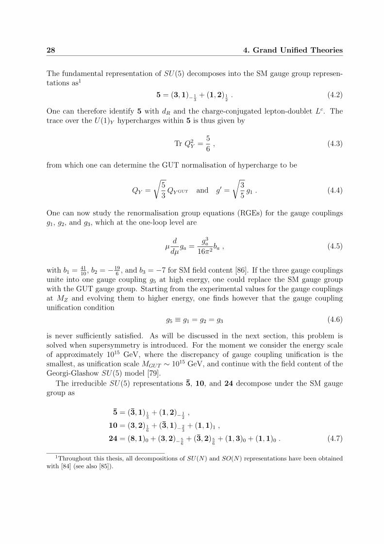
Thus for each generation one can embed the three charge-conjugated down type quarkfields d†R and the lepton-doublet2 L into a joint field F transforming as 5
F =
d†RRd†RBd†RGe−ν
, (4.8)
where R, B, and G denote the three colors of QCD. The remaining matter fields fit intothe antisymmetric 10 as charged-conjugated u†R and e†R, and quark doublet Q
T =1√2
0 −u†RG u†RB −uLR −dLRu†RG 0 −u†RR −uLB −dLB−u†RB u†RR 0 −uLG −dLGuLR uLB uLG 0 −e†RdLR dLB dLG e†R 0
. (4.9)
Right-handed neutrinos can be added as singlet fields, such that neutrino masses can arisevia the see-saw type-I mechanism. It is now easy to understand the origin of U(1)em chargequantisation: When SU(5) gets broken into the SM subgroup, the U(1)Y generator arisesfrom the diagonal SU(5) generator3
T0 =
√3
5diag
(−1
3,−1
3,−1
3,1
2,1
2
), (4.10)
and the QY hypercharges of the SM matter fields emerge from the embedding (4.7) of theSM representation into SU(5) representations. The electric charge operator is
Qe = T3 +
√5
3T0 = diag
(−1
3,−1
3,−1
3, 1, 0
), (4.11)
which explains the fractional electric charge of quarks from the fact that quarks come inthree colours and SU(5) generators are traceless. Overall the peculiar U(1)Y hyperchargeassignment of the SM fields in table 2.1 is strikingly explained when the SM is embeddedinto SU(5).
Note that the Georgi-Glashow model is anomaly free, since the contributions from Fand T to the anomaly coefficients cancel.
The gauge bosons Gµ, Wµ, and Bµ are contained in the adjoint 24. Finally 24 alsocontains twelve additional gauge fields in (3,2)− 5
6and (3,2) 5
6, which do not correspond to
any existing SM field. These new leptoquark gauge bosons are namedX and Y , respectively,
2Note that 5 contains the SU(2) conjugate εL, which explains the sign of ν in (4.8).3The SU(3)C generators are embedded into the 3× 3 upper-left block and the SU(2)L generators into
the 2× 2 lower-right block of the SU(5) generators.

30 4. Grand Unified Theories
and carry SU(2) and SU(3) indices. The Higgs boson φ is supplemented by a new colouredscalar Higgs triplet T (5) and embedded into a fundamental H5
H5 =
T
(5)R
T(5)B
T(5)G
φ+
φ0
. (4.12)
To spontaneously break SU(5) down to the SM subgroup, one introduces a Higgs fieldH24 transforming in the adjoint representation 24, which obtains a vev aligned along thehypercharge direction
〈H24〉 = V diag
(1, 1, 1,−3
2,−3
2
). (4.13)
Equation (4.13) is obtained as global minimum of the most general renormalisable potentialfor the adjoint4
V (H24) = −m224
2TrH2
24 +λ24
4
(TrH2
24
)2+λ′24
4TrH4
24 , (4.14)
when the parameters satisfy m24, λ′24 > 0, and λ24 > − 7
30λ′24. Because 〈H24〉 commutes
with the SU(5) generators of the SM subgroup, the SM gauge group remains unbroken,while the X and Y gauge bosons acquire a heavy mass due to the BEH mechanism
M2X = M2
Y =25
8g2
5V2 . (4.15)
One identifies MX with the mass scale of GUT unification MGUT ≡ MX . Expanding H24
around its vev one finds that twelve degrees of freedom are would-be Goldstone bosonsand absorbed by the massive gauge fields X and Y . The remaining degrees of freedom aretransforming as one SU(3)C octet O(24), one SU(2)L triplet T (24), and one total singletS(24), with masses
m2O(24) =
5
8λ′24V
2 , m2T (24) =
5
2λ′24V
2 , m2S(24) = m2
24 . (4.16)
The full scalar potential also includes the Higgs boson H5 and (4.14) is extended to
V (H24, H†5H5) = V (H24)− µ2
5(H†5H5) + λ5(H†5H5)2
+ λ′H†5H5TrH224 + λ′′H†5H
224H5 . (4.17)
4For simplicity we assume that H24 carries charge 1 under an additional Z2 symmetry, which howeveris not a necessary condition for the potential V to obtain (4.13).
4.1 The Georgi-Glashow SU(5) model 31
With µ5,m24 > 0, λ′24 > 0 > λ′′, λ24 < − 730λ′24, λ′ > − 3
10λ′′, and λ5 >
(λ′ + 3
10λ′′) µ2
5
m224
the
potential (4.17) is minimised by 〈H24〉 and the non-vanishing vev
〈H5〉 =1√2
0000v
, (4.18)
which spontaneously breaks the Electroweak symmetry to U(1)em.5 The two vevs 〈H24〉and 〈H5〉 thus spontaneously break SU(5)→ SU(3)C×U(1)em. The masses of the colouredtriplet T (5) and the SM Higgs boson h are given by
m2T (5) = −5
4λ′′V 2 and m2
h = λ5v2 . (4.19)
In the next section it will be discussed that the coloured triplet T (5) mediates proton decay,which leads to a lower bound of mT (5) & 1012 GeV. The Higgs mass on the other handis mh ∼ 125 GeV, leading to the so-called doublet-triplet splitting (DTS) problem. It isrelated to the hierarchy problem and can be accounted for by a fine-tuning of the potential’sparameters λ′ and λ′′, as can be seen for example from the solution
v2 =µ2
5 −(
304λ′ + 9
4λ′′)V 2
λ5
. (4.20)
In SUSY SU(5) the DTS problem is tightened due to new proton decay mediating operatorsinvolving sparticles. We will return to the DTS problem in section 5.5 and chapter 9.
We close this section with a discussion of the Yukawa sector of the Georgi-Glashowmodel. There are two SU(5) invariant Yukawa operators
LY = −Y5TijF i (H∗5 )j − Y10εijklmTijTkl (H5)m + h.c. , (4.21)
where i, j, . . .m denote SU(5) indices and we have suppressed flavour indices for readability.When SU(5) gets broken (4.21) decomposes into the SM Yukawa interactions
LY = −4Y10Q · φu†R +1√2Y5Q · φ d†R +
1√2Y T
5 L · φ e†R + h.c. , (4.22)
and new Yukawa interactions between the coloured triplet T (5) and the matter fields
LYT (5)
= − 1√2Y5
(Q · L− u†Rd†R
)T (5)∗ − 2Y10
(2u†Re
†R −Q ·Q
)T (5) + h.c. . (4.23)
Comparison with (2.2) gives the following SU(5) GUT scale predictions for the Yukawamatrices
Yd = Y Te , Yu = Y T
u . (4.24)
5〈H5〉 also leads to negligibly small shifts of O (v/V ) in the heavy masses of (4.16).

32 4. Grand Unified Theories
The GUT scale relation Yd = Y Te is however refuted by the observed quark and lepton
masses, when an RG analysis to MGUT is performed. This problem can be solved byadding a new Higgs field H45 transforming as 45 [87]. Under the SM gauge group 45decomposes as
45 = (3,1)− 13
+ (1,2) 12
+ (3,1) 43
+ (3,2)− 76
+ (3,3)− 13
+ (6,1)− 13
+ (8,2) 12, (4.25)
therefore the SM Higgs field φ can be embedded in H45. Writing SU(5) tensor indicesexplicitly, H45 is given by (H45)ijk = − (H45)jik with vanishing trace (H45)iji = 0. When H45
obtains a vev, SU(3)C must not be broken and because of the traceless condition the vevis given by
〈(H45)i5k 〉 = v(δik − 4δi4δk4
)i, k = 1, . . . , 4 , (4.26)
such that the term giving mass to the charged leptons compensates for the number ofcolours. Invoking new global symmetries, one can construct a Lagrange density such thatH45 couples exclusively to the second family
LY ⊃ −ys (T2)ij Fk2 (H∗45)ijk , (4.27)
whereas the remaining matter fields couple to H5.6 The resulting GUT scale Yukawa cou-pling ratios are known as the Georgi-Jarlskog (GJ) relations [87]
yµ = 3ys , ye =1
3yd , (4.28)
where the second relation also requires vanishing 1-1 element of Y5. We will discuss later,that the GJ relations are also challenged by the data today. In section 4.4 we will reviewother predictions for GUT scale Yukawa coupling ratios, when higher-dimensional operatorsinvolving the adjoint are constructed.
The crucial point is that within the framework of GUTs predictions for quark and leptonmass ratios are constructed, setting the stage for flavour models.
4.2 Proton decay in SU(5)
The unification of quarks and leptons into joint representations inevitably enables baryonand lepton number violating operators and thus predicts proton decay. Figure 4.1 showshow exchange of the heavy gauge bosons X and Y leads to baryon number violatingoperators, which can mediate proton decay, like for example p → e+ + π0, as shownin figure 4.2. In the effective theory where the heavy gauge bosons are integrated out,dimension 6 proton decay operators emerge proportional to the SU(5) gauge coupling g5
and MGUT [82]
LB =g2
5
2M2GUT
(u†RσQ · e†RσQ+ u†RσQ · d†RσL
). (4.29)
6Because of the additional shaping symmetries, in flavour GUT models several H5’s might be required.

4.2 Proton decay in SU(5) 33
X
uL
u†R
e†L
dR
Y
uL
dL
e†R
u†R
Y
uL
dL
ν†L
d†R
Figure 4.1: Baryon number violating operators mediating proton decay due to heavygauge boson exchange.
p
u
u
d
e+
d
π0
X
Figure 4.2: Feynman diagram for the proton decay p → e+π0 mediated by the heavygauge boson X.
The amplitude for proton decay depends on the RG evolution and the quark and leptonmixing matrices. Based on dimensional analysis there is a model-independent estimate forthe proton decay rate
Γp ≈ α25
m5p
M4GUT
, (4.30)
where α5 ≡ g25
4π2 and mp ∼ 938 MeV is the proton mass. The most stringent bound on theproton lifetime is τ (p→ e+ + π0) > 8 · 1033 years [14], which yields a lower bound for theGUT scale of
MGUT & 1016 GeV , (4.31)
for α5 ≈ 125
. The too high proton decay rate predicted by the unification scale MGUT =1015 GeV is another problem that can be elegantly solved in SUSY SU(5), where theunification scale can easily be above 1016 GeV, as discussed in 5.5 and 9.3.
Besides the heavy X and Y bosons, also the colour triplet T (5) can mediate proton decayvia the Yukawa couplings to quarks and leptons shown in (4.23) and figure 4.3. Like forthe heavy gauge boson mediated proton decay, the decay rate is flavour model dependent.Again an estimate based on dimensional grounds is [82]
Γp ≈ |yuyd|2m5p
m4T (5)
, (4.32)
where yu and yd are the Yukawa couplings of the first generation quarks. The lower boundfor the mass of the coloured triplet is then given by
mT (5) > 5 · 1011 GeV , (4.33)

34 4. Grand Unified Theories
T (5)
uL
dL
eL
uL
Figure 4.3: Example for a baryon violating operator mediating proton decay through aheavy coloured triplet.
with yuyd ≈ 4 · 10−10. Thus we have identified the root of the doublet-triplet splittingproblem, in order to prevent too rapid proton decay the triplet in H5 has to be manyorders of magnitude heavier than the doublet, whose mass is at the electroweak scale.
4.3 Pati-Salam unification and SO(10)
The main part of this thesis is dedicated to SUSY flavour models in SU(5) grand unifica-tion. We therefore only briefly discuss unification in Pati-Salam (PS) [88] and SO(10) [89]gauge groups in this section.
The Pati-Salam gauge group is SU(4)C × SU(2)L × SU(2)R with the underlying ideato identify leptons as fourth colour of SU(4)C . The SM matter content can be embeddedinto two representations QL and QR transforming as (4,2,1) and (4,1,2), respectively.Under the SM gauge group they decompose as
(4,2,1) = (3,2) 16
+ (1,2)− 12
(4,1,2) = (3,1) 13
+ (3,1)− 23
+ (1,1)1 + (1,1)0 . (4.34)
Therefore the SM SU(2)L doublets Q and L are embedded into QL and the charge-conjugated fields u†R, d†R, and e†R are embedded into QR. The multiplet QR is completedwith a SM singlet field, which can be identified with the charge-conjugate of a heavy right-handed neutrino ν†R. Thus massive neutrinos arise as prediction from PS unification. TheSM Higgs doublet is contained in H, transforming as
(1,2,2) = (1,2) 12
+ (1,2)− 12. (4.35)
The most general renormalisable Yukawa interaction Lagrange density in PS is thus
LYPS = −YPSQLHQR . (4.36)
When the PS gauge group is broken to the SM, this gives rise to the (very bad) GUT scalepredictions
Yu = Yd = Ye = Yν . (4.37)
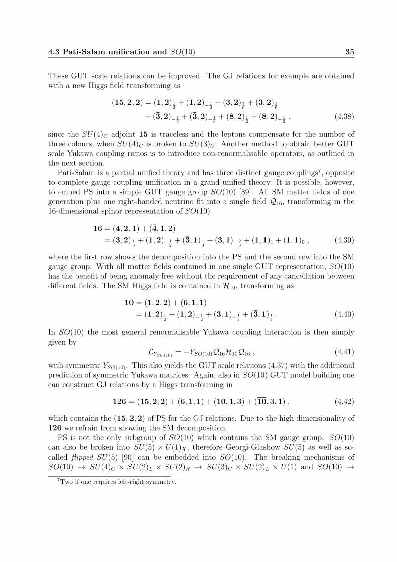
4.3 Pati-Salam unification and SO(10) 35
These GUT scale relations can be improved. The GJ relations for example are obtainedwith a new Higgs field transforming as
(15,2,2) = (1,2) 12
+ (1,2)− 12
+ (3,2) 76
+ (3,2) 16
+ (3,2)− 76
+ (3,2)− 16
+ (8,2) 12
+ (8,2)− 12, (4.38)
since the SU(4)C adjoint 15 is traceless and the leptons compensate for the number ofthree colours, when SU(4)C is broken to SU(3)C . Another method to obtain better GUTscale Yukawa coupling ratios is to introduce non-renormalisable operators, as outlined inthe next section.
Pati-Salam is a partial unified theory and has three distinct gauge couplings7, oppositeto complete gauge coupling unification in a grand unified theory. It is possible, however,to embed PS into a simple GUT gauge group SO(10) [89]. All SM matter fields of onegeneration plus one right-handed neutrino fit into a single field Q16, transforming in the16-dimensional spinor representation of SO(10)
16 = (4,2,1) + (4,1,2)
= (3,2) 16
+ (1,2)− 12
+ (3,1) 13
+ (3,1)− 23
+ (1,1)1 + (1,1)0 , (4.39)
where the first row shows the decomposition into the PS and the second row into the SMgauge group. With all matter fields contained in one single GUT representation, SO(10)has the benefit of being anomaly free without the requirement of any cancellation betweendifferent fields. The SM Higgs field is contained in H10, transforming as
10 = (1,2,2) + (6,1,1)
= (1,2) 12
+ (1,2)− 12
+ (3,1)− 13
+ (3,1) 13. (4.40)
In SO(10) the most general renormalisable Yukawa coupling interaction is then simplygiven by
LYSO(10)= −YSO(10)Q16H10Q16 , (4.41)
with symmetric YSO(10). This also yields the GUT scale relations (4.37) with the additionalprediction of symmetric Yukawa matrices. Again, also in SO(10) GUT model building onecan construct GJ relations by a Higgs transforming in
126 = (15,2,2) + (6,1,1) + (10,1,3) + (10,3,1) , (4.42)
which contains the (15,2,2) of PS for the GJ relations. Due to the high dimensionality of126 we refrain from showing the SM decomposition.
PS is not the only subgroup of SO(10) which contains the SM gauge group. SO(10)can also be broken into SU(5) × U(1)X , therefore Georgi-Glashow SU(5) as well as so-called flipped SU(5) [90] can be embedded into SO(10). The breaking mechanisms ofSO(10) → SU(4)C × SU(2)L × SU(2)R → SU(3)C × SU(2)L × U(1) and SO(10) →
7Two if one requires left-right symmetry.

36 4. Grand Unified Theories
SU(5) × U(1)X → SU(3)C × SU(2)L × U(1) are rather complicated and involve severalGUT-breaking Higgs fields. Since the flavour models in the main part of this thesis areSU(5) GUTs, the details of SO(10) and subsequently PS breaking are of no relevance forthis thesis and therefore not discussed.
4.4 GUT scale Yukawa coupling ratios
The SU(5) and PS predictions of Ye = Y Td and Ye = Yd = Yu, respectively, are highly
disfavoured by experimental results, when the RG evolution of the particle masses (orrather their Yukawa couplings) to the GUT scale is studied.8 A convenient test whetherGUT predictions for the first two families are consistent with the experimental data isprovided by the - RG invariant and SUSY threshold correction invariant9 - double ratio [91]∣∣∣∣yµ ydys ye
∣∣∣∣ ≈ 10.7+1.8−0.8 . (4.43)
Thus also the GJ relations (4.28) are in tension with experimental observations, since theyyield a double ratio of 9 and thus deviate from the constraint (4.43) by more than twosigma.
The problem of poor GUT scale predictions can be solved when the Yukawa couplings areeffective higher-dimensional operators, containing a GUT breaking Higgs field. When theGUT gauge group gets spontaneously broken to the SM, new GUT scale Yukawa couplingratios arise due to the appearance of group theoretical Clebsch-Gordan (CG) factors [83].
R
A
B
C
D
R
A
B
C
D
Figure 4.4: Feynman diagrams with heavy messenger fields R give rise to the effectivedimension 5 operators ABCD, thereby new GUT-scale predictions for the Yukawa couplingratios arise from group-theoretical CG factors.
Generally, in a higher-dimensional operator involving GUT non-singlet fields there areseveral possibilities how the GUT group indices are contracted to form a gauge singlet,yielding a non predictive, arbitrary linear combination of multiple CG factors. For examplein SU(5) GUTs the dimension five operator FT (H5)∗H24 yields a linear combination ofthe GUT scale Yukawa couplings ratios 1 and −3. In order to restore predictivity in a
8SUSY threshold effects in RG analyses are discussed in section 5.4 and chapter 10.9As long as the first two families of sfermions are almost degenerate in mass, as commonly assumed.

4.4 GUT scale Yukawa coupling ratios 37
specific flavour GUT model, one therefore must introduce heavy messenger fields in GUTnon-singlet representations, which UV complete the model at high energy and single outa specific GUT index contraction. This guarantees that only an unique effective operatorwith defined CG factor is constructed in the effective theory, when the heavy messengerfield is integrated out. Figure 4.4 shows the two Feynman diagrams yielding predictiveeffective dimension five operators. In table 4.1 some examples are shown for the case of anSU(5) GUT. If for example the effective operator FT (H5)∗H24 is obtained via a messenger
AB C D R (Ye)ji/(Yd)ij
F T H∗5 H24 5 1
F T H∗5 H24 45 −3
H24F T H∗45 45 −12
H24F T H∗5 5 −32
H24 T F H∗5 10 6
Table 4.1: CG factors for the dimension five effective operators from figure 4.4. The upperpart corresponds to the left diagram, the lower one to the right one. See the main text fordetails.
field ΦR transforming as 45
L ⊃ −λFT ΦR −mH∗5H24Φ∗R −m2ΦR
ΦRΦ∗R , (4.44)
the unique CG factor −3 arises as prediction for the GUT scale Yukawa coupling ratios.If one would use instead a messenger field transforming as 5, one would obtain the CGfactor 1.
In table 4.1 we have also listed the SU(5) CG factors −12, −3
2, and 6, since they are of
special importance in the main part of this thesis. The full list of possible CG factors ciin SU(5) is given by [83]
ci ∈ −1
2, 1,±3
2,−3,
9
2, 6, 9,−18 . (4.45)
In PS partial unification one also finds CG factors for the Yukawa coupling ratios(Ye)ij/(Yd)ij, as well as (Yu)ij/(Yd)ij from higher-dimensional operators. An extensive listof CG predictions from dimension 5 and dimension 6 operators in PS embedded in SO(10)is found in [83] (see also [92]). We will be only interested in the relations between Ye andYd in PS, for which for example the CG factors
ci ∈ 3
4, 1, 2,−3, 9 (4.46)
are available.

38 4. Grand Unified Theories
In a recent paper [93] further new CG factors were obtained, by replacing the massesof the messengers fields with vevs from non-singlet fields. These new CG factors for Ye/Ydare given by
ci ∈−2
3, 1
6 in SU(5) ,
−13, 0, 3
2 in PS .
(4.47)
Utilising CG factors for quark and lepton Yukawa coupling ratios will be an essentialconcept in the flavour GUT models of this thesis.

CHAPTER 5
Supersymmetry
The Georgi-Glashow SU(5) model beautifully unifies the SM matter fields into the jointrepresentation F and T , enabling the construction of predictions for quark - lepton Yukawacoupling ratios. There are two problems however: Firstly the SM gauge couplings neverunite satisfactory, and secondly there is the prediction of too rapid proton decay due toheavy gauge boson mediation. Remarkably, both problems can be solved at once with theintroduction of supersymmetry (SUSY).
In a nutshell, SUSY is a symmetry transforming fermions into bosons and vice versa.The minimal supersymmetric Standard Model (MSSM) predicts the existence of a scalarparticle for each SM fermion and a Majorana fermion for each gauge boson of the SM.When these additional supersymmetric partners (sparticles) of the SM particles have nottoo heavy masses, the MSSM gauge couplings successfully unify at a GUT scale highenough to sufficiently suppress proton decay. Additionally SUSY provides a solution tothe hierarchy problem and a candidate particle for dark matter.
In this chapter N = 1 supersymmetry and SUSY SU(5) are reviewed, following thepresentations of [81, 94–99].
5.1 The Wess-Zumino model
The simplest supersymmetric quantum field theory with minimal field content is givenby the Wess-Zumino (WZ) model [100]. A supersymmetric theory must contain the samenumber of fermionic and bosonic degrees of freedom (d.o.f.). In four-dimensional spacetimethe smallest fermionic representation is a two-component Weyl spinor ψ. On-shell, ψsatisfies the Dirac equation iσµ∂µψ = mψ†, which eliminates two of ψ’s four real d.o.f. Acomplex scalar field φ is thus enough to balance the number of fermionic and bosonic d.o.f.on-shell. The superpartners ψ and φ form a chiral supermultiplet. Finally, to match thefermionic d.o.f. also off-shell, an auxiliary complex scalar field F with two non-physical

40 5. Supersymmetry
d.o.f. is additionally introduced. The Wess-Zumino Lagrange density of ψ, φ, and F is
LWZ = iψ†σµ∂µψ + ∂µφ∂µφ∗
− 1
2
(mψψ +m∗ψ†ψ†
)− 1
4
(yφψψ + y∗φ∗ψ†ψ†
)+ FF ∗ + F
(mφ+
y
2φ2
)+ F ∗
(m∗φ∗ +
y∗
2φ∗2). (5.1)
There is no kinetic term for the auxiliary field F , since it does not propagate a physicald.o.f. It can thus be integrated out yielding the scalar potential
VWZ(φφ∗) = FF ∗ = m2φφ∗ +
(my∗
2φφ∗2 +
my
2φ∗φ2
)+yy∗
4(φφ∗)2 . (5.2)
LWZ is invariant under the supersymmetry transformation
δφ = εψ , δφ∗ = ε†ψ† ,
δψ = −iσµε†∂µφ+ εF , δψ† = iεσµ∂µφ∗ + ε†F ∗ ,
δF = −iε†σµ∂µψ , δF ∗ = i∂µψ†σµε , (5.3)
where ε is a two-component spinor, anti-commuting, and the infinitesimal supersymmetrytransformation parameter.1 The mass dimension of ε is −1
2. Requiring invariance under
(5.3) is the reason why the couplings for all terms in LWZ and VWZ are given only by thetwo parameters m and y.
Using a Wess-Zumino chiral multiplet, one can now present in a simplified manner howSUSY yields a solution to the hierarchy problem. Taking m in (5.1) to be due to the Higgsvev m→ λ√
2(v + h) one finds the couplings
− λ
2√
2
(hψψ + hψ†ψ†
), −λ
2
2h2φφ∗ , and − λ2vhφφ∗ , (5.4)
between the real scalar Higgs boson h and the WZ component fields ψ and φ. The Higgsself-energy contribution from the fermion loops shown in figure 5.1 is quadratically diver-gent
Π(f)hh (0) = (−1)λ2
∫d4k
(2π)4
1
k2 −m2+
2m2
(k2 −m2)2 , (5.5)
and independent of the Higgs mass mh. We know that if the SM is embedded into aGUT, there are particles with m ∼ MGUT in the spectrum, which yields the hierarchyproblem2: There must be a fine-tuning in the renormalisation of the quadratic divergence
1We limit our discussion to the case of global SUSY, where ε is independent of xµ.2The hierarchy problem is not specific to GUTs but appears whenever new (non-sypersymmetric)
physics at high scales is introduced.

5.1 The Wess-Zumino model 41
h h
ψ
ψ†
ψ†
ψh h
ψ†
ψ†
ψ†
ψ†
h h
ψ
ψ
ψ
ψ
Figure 5.1: The Feynman diagrams contributing to the Higgs self-energy via a fermionloop. Note that for Weyl fermions the arrows on the propagators do not correspond tocharge or momentum (see e.g. [12]).
h h
φ∗
φ∗
φ
φ
h hφ∗ φ
Figure 5.2: The Feynman diagrams contributing to the Higgs self-energy via the scalarsuperpartner φ.
of 1 in 1028 since mh ∼ O(100 GeV). In supersymmetry, however, the contribution to theHiggs self-energy from the superpartner φ loops in figure 5.2 give
Π(b)hh(0) = λ2
∫d4k
(2π)4
1
k2 −m2+
2m2
(k2 −m2)2 , (5.6)
and thus precisely cancels the fermionic contributions. This is true to all orders in pertur-bation theory.
There is no evidence for scalar particles with the same masses as the SM fermions,therefore SUSY has to be broken. In order to keep the cancellation of the quadraticdivergence, only soft SUSY breaking terms are allowed. For example a small mass squareddifference δ between ψ and φ yields
Π(b)hh(0) ' λ2
∫d4k
(2π)4
1
k2 −m2+
2m2
(k2 −m2)2 +2δ2
(k2 −m2)2 , (5.7)
such that only a logarithmic divergence ofO(δ2 log m2
µ2
)remains. Supersymmetry breaking
will be discussed in 5.3.We close this section by a discussion of gauge supermultiplets. The superpartner of a
gauge boson Aaµ is a two-component spin 12
gaugino λa. Like for the WZ supermultiplet,one introduces a real auxiliary scalar field Da to manifest SUSY off-shell.3 All components
3We give the expressions in Wess-Zumino gauge [101].
42 5. Supersymmetry
of the gauge supermultiplet transform in the same representation of the gauge group. TheLagrange density for the gauge supermultiplet is given by
Lgauge = −1
4F aµνF
µνa + iλa†σmuDµλa +
1
2DaDa , (5.8)
with the gauge covariant derivative for the gaugino
Dµλa = ∂µλ
a + gfabcAbµλ
c . (5.9)
The SUSY transformations are given by
δAaµ = − 1√2
(ε†σµλ
a + λa†σµε),
δλa =i
2√
2σµσνεF a
µν +1√2εDa ,
δDa =i√2
(−ε†σµDµλ
a +Dµλa†σµε
). (5.10)
Finally the coupling of the WZ supermultiplet to the gauge supermultiplet is given by theadditional terms
−√
2g (φ∗T aψ)λa , −√
2gλa†(ψ†T aφ
), g (φ∗T aφ)Da , (5.11)
where additionally in (5.3) the ordinary derivatives have to be replaced by gauge co-variant ones and the transformations δF and δF ∗ get extra terms +
√2g (T aφ) ε†λa† and
+√
2gλaε (T aφ∗), respectively. The auxiliary field Da can be integrated out and the scalarpotential gets a D-term contribution in addition to the F-term (5.2)
V (φ, φ∗) = FF ∗ +1
2DaDa . (5.12)
Note that V (φ, φ∗) is strictly non-negative. In section 5.3 it will be shown that in SUSYtheories the vacuum energy is always zero.
5.2 Superspace and Superfields
A simple formalism for supersymmetric theories can be be achieved be introducing super-space [102]. In addition to the spacetime coordinate xµ, superspace is spanned by twoanti-commuting two-component spinors θ and θ†. The mass dimension of θ and θ† is −1
2.
Superfields are functions of xµ, θ, and θ† and unite the component fields of a supermulti-plet. Because θ and θ† are Grassmann variables, an expansion of a general superfield in θand θ† terminates
S(xµ, θ, θ†) = φ+ θξ + θ†χ† + θθF
+ θ†θ†ρ+ θ†σµθVµ + θ†θ†θη + θθθ†ζ† + θθθ†θ†δ , (5.13)
5.2 Superspace and Superfields 43
where φ, F , ρ, δ are complex scalar fields, Vµ is a complex vector boson, and ξ, χ†, η, andζ† are two-component Weyl fermions. Thus, the number of bosonic and fermionic d.o.f.match.
In analogy with the gauge covariant derivative Dµ one introduces the chiral covariant
derivatives Dα and D†α in superspace, which are SUSY covariant
Dα =∂
∂θα− i(σµθ†
)α∂µ , D†α =
∂
∂θ†α+ i (θσµ)α ∂µ . (5.14)
One can now prescribe constraints on a general superfield S to reduce the total number of32 degrees of freedom to the small number of d.o.f. in the WZ supermultiplet. Imposing
D†αΦ = 0 (5.15)
yields a left-chiral superfield
Φ(xµ, θ, θ†) = φ(x) +√
2θψ(x) + θθF (x)
+ iθ†σµθ∂µφ(x) +1
4θθθ†θ†∂µ∂
µφ(x)− i√2θθθ†σµ∂µψ(x) , (5.16)
which contains the component fields of the WZ supermultiplet. It’s complex conjugate Φ∗
satisfying DαΦ∗ = 0 is named right-chiral. Chiral superfields have mass dimension one.Starting from several left-chiral superfields Φi one can build a new left-chiral superfieldfrom a holomorphic4 function W(Φi).
ImposingV = V ∗ (5.17)
yields a vector superfield
V (xµ, θ, θ†) = φ(x) + θξ(x) + θ†ξ†(x) + θθF (x) + θ†θ†F ∗(x)
+ θ†σµθVµ(x) + θ†θ†θη(x) + θθθ†η†(x) + θθθ†θ†δ(x) , (5.18)
where φ, δ, and Aµ are now real fields. One can construct a vector superfield from chiralfields by e.g. Φ + Φ∗ and Φ∗Φ.
Whenever V is the vector superfield to a gauge symmetry it transforms as
e2gV → e−2igΛ∗e2gV e2igΛ , (5.19)
where V ≡ V aT a, Λ ≡ ΛaT a, T a are the generators of the gauge group, and Λa is a chiralsuperfield and the supergauge transformation parameter. Ordinary gauge transformationare obtained as special case when Λ is restricted to its scalar component. The chiralsuperfields transform under the supergauge symmetry as
Φ→ e−2igΛΦ , Φ∗ → e2igΛ∗Φ∗ . (5.20)
4Here holomorphic refers to the complex scalar component fields φi of Φi.
44 5. Supersymmetry
For an Abelian gauge symmetry the supergauge transformation for V simplifies to
V → V + i (Λ− Λ∗) . (5.21)
One can now use this freedom to make a suitable supergauge transformation and bring(5.18) into Wess-Zumino gauge
V (xµ, θ, θ†) = θ†σµθAµ(x) + θ†θ†θλ(x) + θθθ†λ†(x) +1
2θθθ†θ†D(x) . (5.22)
In WZ gauge it is easily recognised that V is dimensionless, justifying the eV terms above.It is very useful to note that due to the Grassmann characteristics of θ and θ† the expansionseries of eV terminates
e2gV = 1 + 2gV + 2g2V 2
= 1 + 2g
(θσµθ†Aµ + θθθ†λ† + θ†θ†θλ+
1
2θθθ†θ†D
)+ g2θθθ†θ†AµA
µ . (5.23)
One can construct chiral spinorial field strength superfields
Wα = −1
4D†D†e−2gVDαe
2gV , W †α = −1
4DDe2gVD†αe
−2gV , (5.24)
which transform as
Wα → e−2igΛWαe2igΛ , W †
α → e2igΛ†W †αe−2igΛ† , (5.25)
under supergauge transformations.
In superspace formalism the Lagrange density is obtained from integrating a vectorsuperfield over the Grassmann coordinates θ and θ†
L = [V ]D ≡∫d2θ
∫d2θ† V (xµ, θ, θ†) =
1
2D + . . . , (5.26)
which is supersymmetric invariant since the D-term transforms into a total derivativeunder SUSY transformations (5.10) and . . . represents a total derivative term which is ofno importance in L. Another SUSY invariant term is the F -term of a chiral superfieldgauge singlet, which also transforms into a total derivative under SUSY (5.3)
[Φ]F ≡∫d2θΦ(xµ, θ, θ†) = F . (5.27)
The Lagrange density can then be built from
L = [Φ]F + h.c. (5.28)

5.2 Superspace and Superfields 45
A general supersymmetric Lagrange density can thus be built out of chiral and vectorsuperfields as
LSUSY =
[K(Φ∗i e
2gV Φj
)+ 2κV
]D
+
([1
4fab (Φi)W
aW b +W (Φi)
]F
+ h.c.
), (5.29)
where i, j denote generation indices, a, b are indices of the adjoint representation of thegauge group, and we introduced the following quantities:
Kahler potential K of left-chiral, right-chiral, and vector superfields. K is real andhas mass dimension two. In the renormalisable case it is simply given by Φ∗i e
2gV Φi =Φ∗Φ + 2gΦ∗V Φ + 2g2Φ∗V 2Φ and it’s D-term yields the kinetic energy terms of the matterfields
LK = (Dµφi)†Dµφi + iψ†i σ
µDµψi + FiF∗i
−√
2g (φ∗T aψλa + h.c.) + g (φ∗T aφ)Da . (5.30)
In global SUSY the Kahler potential is invariant under the transformation
K → K + F (Φi) + F ∗(Φ∗i ) , (5.31)
with F a holomorphic function of Φi. All holomorphic and antiholomorphic functions cantherefore be removed from the Kahler potential.
Fayet-Iliopoulos (FI) term 2κ[V ]D [103] in the case of an Abelian gauge group, sincethe D-term of a gauge singlet V is gauge invariant.
LFI = κD . (5.32)
The FI term does not exist for vector bosons of non-Abelian gauge groups.
gauge kinetic function fab, a dimensionless chiral superfield and holomorphic functionof chiral superfields. In renormalisable theories fab is simply given by δab + igaθa
8π2 δab, suchthat the F -terms yield the usual gauge kinetic energy plus in the case of a non-Abeliangauge symmetry a potentially topologically non-trivial θ term
Lgauge = −1
4F aµνF
µνa − g2aθ
64π2εµνλρF
λρaF µνa + iλaσµDµλa† +
1
2DaDa . (5.33)

46 5. Supersymmetry
superpotential W , a holomorphic function of left-chiral superfields. It has mass dimen-sion three and for renormalisable Lagrange densities it is given by
W(Φi) = LiΦi +1
2MijΦiΦj +
1
6YijkΦiΦjΦk , (5.34)
where the first term vanishes for non gauge singlet superfields Φi. The F -term [W (Φi)]F +h.c. yields mass terms and Yukawa couplings
L =W iFi −1
2W ijψiψj + h.c.
=
(Li +Mijφj +
1
2Yijkφjφk
)Fi −
1
2(Mij + Yijkφk)ψiψj + h.c. , (5.35)
where the notation
Wi ≡∂W∂Φi
∣∣∣∣θ=θ†=0
, Wij ≡∂2W∂Φi∂Φj
∣∣∣∣θ=θ†=0
(5.36)
was introduced which indicates that we set θ = θ† = 0 after differentiation, such thatonly the scalar components remain. Similarly we define W∗i and W∗ij for the conjugatesuperpotential W∗ (Φ∗).
Like mentioned above, the auxiliary fields Fi and Da do not propagate a physical d.o.f.and can be integrated out to yield the scalar potential
V (φ, φ∗) =WiW∗i +1
2
∑a
∣∣gaφ†T aφ+ κa∣∣2 , (5.37)
where for non-Abelian gauge symmetries κa = 0.For non-renormalisable SUSY theories it is convenient to introduce supergraphs [104]
(see e.g. [97,105] for a review). When heavy particles are integrated out from a renormalis-able theory, a non-renormalisable Kahler potential and a non-renormalisable superpotentialemerge in the effective theory, as shown in figure 5.3. After the heavy superfields Φn areintegrated out, the terms
YijnYklnMnn
ΦiΦjΦkΦl andYijnY
∗kln
M2nn
ΦiΦjΦ∗kΦ∗l (5.38)
appear in the superpotential and Kahler potential, respectively. Note that one can easilyobtain the effective Kahler potential by cutting a propagator in the supergraph of aneffective superpotential term in half, “flip” one side to the charge-conjugated expressionand stitch the resulting parts together. From the Kahler potential one can define theKahler metric5
Kji ≡
∂2
∂Φi∂Φ∗j
∣∣∣∣θ=θ†=0
, (5.39)
5Here we use the convention that lower indices correspond to derivatives with respect to left-chiralsuperfields and upper indices to derivatives with respect to their complex conjugated (right-chiral) super-
fields, e.g.(Kji
)∗= Ki
j .

5.2 Superspace and Superfields 47
Φn
Φi
Φj
Φk
Φl
Φn
(a)
Φ∗n
Φi
Φj
Φ∗k
Φ∗l
Φn
(b)
Figure 5.3: Supergraphs for non-renormalisable superpotential (a) and non-renormalisable Kahler potential (b).
with the inverse (K−1)ij satisfying (K−1)
ijK
kj = δkj . Mathematically this means that the
chiral fields are defined on a Kahler manifold and one can calculate the connection
Γkij =(K−1
)knKnij , (5.40)
and Riemann curvature tensor
Rjlik = Kjl
ik −(K−1
)nmKmikK
jln , (5.41)
where
Kkij ≡
∂3
∂Φi∂Φj∂Φ∗k
∣∣∣∣θ=θ†=0
, and Kklij ≡
∂4
∂Φi∂Φj∂Φ∗k∂Φ∗l
∣∣∣∣θ=θ†=0
. (5.42)
The on-shell Lagrange density for the matter component fields after integrating out theauxiliary fields F and Da can than be expressed as
Lmatter = KjiDµφi (D
µφj)∗ + iKj
i ψ†j σ
µDµψi
− 1
2
(Wijψiψj − ΓkijWkψiψj + h.c.
)+
1
4Rjlikψiψkψ
†jψ†l
−(K−1
)ijWiW∗j −
1
2
∑a
∣∣∣gaφ†iT aKi + κa∣∣∣2 , (5.43)
where the covariant derivative of the fermion fields includes the connection
Dµψ = ∂µψ − igV aµ T
aψ + Γiij∂µφjψk , (5.44)
and we introduced
Ki ≡ ∂K
∂Φ∗i
∣∣∣∣θ=θ†=0
. (5.45)
For non-trivial Kahler metric Kji 6= δji the kinetic terms in (5.43) have to be brought into
canonical form via canonical normalisation (CN) [106]. The CN procedure transforms thesuperfields Φ→ P−1
Φ Φ such that Kji is diagonalised and rescaled [107,108]
P †ΦKPΦ = 1 , (5.46)

48 5. Supersymmetry
where the most general form of PΦ is given by
PΦ = U †Φ
(√Kdiag
)−1
U , with UΦKU†Φ = Kdiag . (5.47)
The unitary matrix U can be chosen arbitrarily and allows to set PΦ hermitean. Rescalingthe superfields in CN also affects masses and Yukawa couplings in the effective superpo-tential. In flavour models Yukawa couplings emerge from non-renormalisable operatorswhen flavon fields obtain their vevs. Therefore, in SUSY flavour models, the effective su-perpotential for the Yukawa couplings will always adjoin an effective Kahler potential asdescribed below (5.38). Explicit SUSY flavour models thus have to either guarantee thatthe CN effects are negligible (Kj
i ≈ δji in the effective theory) or otherwise the sizeable CNcorrections need to be carefully included into the model’s predictions [107,108].
We close this section by briefly discussing R-symmetries. A global U(1)R symmetry isdefined by the transformation of the anti-commuting coordinates θ and θ†
θ → eiαRθ , and θ† → e−iαRθ† . (5.48)
The Lagrange density can be invariant under U(1)R when R-charges RΦ are assigned toeach superfield. A general superfield S(xµ, θ, θ†) transforms as
S(xµ, θ, θ†)→ eiαRΦS(xµ, e−iαθ, eiαθ†) . (5.49)
The components of a chiral superfield Φ transform with R-charges R(φ) = RΦ, R(ψ) =RΦ − 1, and R(F ) = RΦ − 2. To build an U(1)R invariant Lagrange density the superpo-tential must carry R-charge R(W) = 2, thus the form of the most general superpotential(5.34) gets constrained. A vector superfield V always has R-charge zero, therefore the corre-sponding (gauge-independent) R-charges of its component fields are R(Aµ) = 0, R(λ) = 1,and R(D) = 0. A gaugino mass term −1
2Mλaλa has R-charge two and therefore not only
breaks SUSY, but also U(1)R. Discrete Zn are also candidates for R-symmetries, withR-parity Z2
R conventionally assigned to the superfields in such a way that SM particleshave R-parity +1 and sparticles have R-parity −1. If R-parity is an unbroken symmetryof nature, the lightest supersymmetric paricle (LSP) is stable and therefore a promisingcandidate for Dark Matter.
5.3 Supersymmetry breaking
As discussed at the beginning of this chapter, supersymmetry has to be a broken symmetryof nature, since there is no evidence for the existence of the the charged leptons’ superpart-ners. There are two ways SUSY can be broken: spontaneously via non-vanishing vevs andexplicitly. We start the discussion with spontaneous SUSY breaking and look at the SUSYtransformations of the component fields of a general vev. Because of Lorentz invariance,only scalar fields can have non-vanishing vevs, fermion fields and field derivatives must

5.3 Supersymmetry breaking 49
vanish. From Eqs. (5.3) and (5.10) it follows
δ〈φi〉 = 0 , δ〈ψi〉 ∼ ε〈Fi〉 , δ〈Fi〉 = 0 ,
δ〈Aaµ〉 = 0 , δ〈λa〉 ∼ ε〈Da〉 , δ〈Da〉 = 0 . (5.50)
Therefore a vev is only SUSY invariant if and only if 〈Fi〉 = 0 and 〈Da〉 = 0. Consequently,from (5.12), a supersymmetric vacuum has zero energy.6 In order to break SUSY sponta-neously one needs to assure that either 〈Fi〉 6= 0 or 〈D〉 6= 0 via an F-term SUSY breakingor D-term SUSY breaking mechanism, respectively.F -term SUSY breaking requires that the global minimum of the scalar potential develops
a vev such that 〈Fi〉 = 0 can not be simultaneously satisfied for all Fi. Thus the superpoten-tial for F -term SUSY breaking needs to contain a linear term of a gauge singletW ⊃ LiΦi
since otherwise F ∗i = −Wi has always a vanishing solution with 〈φi〉 = 0. The sim-plest F -term breaking mechanism of interacting superfields is given by the O’Raifeartaighmodel [109]
WO’Raifeartaigh = mΦ2Φ3 + λΦ1
(Φ2
3 − µ2), (5.51)
with real m, λ, and µ. The F -terms are given by
F1 = −λ(φ∗3 − µ2
), F2 = −mφ∗3 , andF3 = −mφ∗2 − λφ∗1φ∗3 . (5.52)
Since F1 = 0 and F2 = 0 are impossibly simultaneously satisfied, one F -term has to obtaina vev and SUSY is spontaneously broken.D-term SUSY breaking emerges from a non-vanishing vev of a D-term component of a
vector superfield, which has to be a gauge singlet due to gauge invariance of the Lagrangedensity. The simplest model for D-term SUSY breaking is due to Fayet-Iliopoulos [103]
VFI(φ, φ∗) =
1
2
(κ+ gq|φ|2
)2. (5.53)
If κq > 0 no vev of φ can achieve vanishing scalar potential, the minimum of V is given by12κ2 at 〈φ〉 = 0, therefore the D-term is given by
D = −κ , (5.54)
and SUSY is spontaneously broken.That SUSY is broken by non-vanishing vevs of the auxiliary F and D component fields
can also be noticed from the fact that 〈F 〉 and 〈D〉 induce mass terms for the scalarparticles and therefore introduce a mass splitting between scalar and fermion components.A general sum rule for the masses of fermions and bosons can be derived from the massmatrices of scalars
M2S =
(W∗ikWkj +DaiDaj +Dai
j Da W∗ijkWk +DaiDaj
WijkW∗k +DaiD
aj WikW∗kj +Da
iDaj +Daj
i Da
)(5.55)
6More technical this can be derived by the N = 1 SUSY algebra Qα, Q†β = 2σµαβPµ, Qα, Qβ =
Q†α, Q†β = 0, where the generators of SUSY transformation Q and Q† are Weyl spinors and the Hamil-
tonian is given by H = P0 = 14 (Q1, Q
†1+ Q2, Q
†2).

50 5. Supersymmetry
where we defined Dai = ∂
∂ΦiDa∣∣∣θ=θ†=0
, the mass matrix of fermions
MF =
(Wij −
√2Da
i
−√
2Daj 0
), (5.56)
and the mass matrix of massive vector bosons emerging from some non-vanishing vev 〈φi〉and the BEH-mechanism
M2abV =
(DaiD
bi +DaiDbi
). (5.57)
The result is the so-called supertrace [110]
STr(M2)
=1∑
J=0
(−1)2J(2J + 1)M2J = −2gaTr (T a〈Da〉) , (5.58)
which holds in spontaneously broken and unbroken SUSY, and the RHS vanishes for non-anomalous U(1) such as the U(1)Y in the MSSM. Analogous to Goldstone’s theorem forbosonic symmetries, the spontaneous breaking of global SUSY yields the Goldstino [103,111], a massless Majorana fermion, which is proportional to the fermionic partners of theauxiliary fields obtaining a vev7
ψG ∼ 〈Fi〉ψi +1√2〈Da〉λa . (5.59)
Phenomenological constraints such as the supertrace (e.g. 2m2e = m2
e1+m2
e2for vanishing
lepton flavour mixing) or the fact that an U(1)Y FI term would spontaneously breakSU(3)C or U(1)em necessitate SUSY breaking in a hidden sector, rather than superfieldsof known SM particles. For this purpose it is useful to investigate soft explicit SUSYbreaking first. A SUSY breaking term in the Lagrange density is named soft if it is atmost logarithmically divergent and therefore does not reintroduce the hierarchy problem. Anecessary but not sufficient condition is that soft terms must not have mass dimension largerthan three [112]. To all orders in perturbation theory, a general soft-breaking Lagrangedensity is given by [113]
Lsoft = −1
2Maλ
aλa + h.c.−m2ijφ∗iφj
−(hiφi +
1
2bijφiφj +
1
6aijkφiφjφk + h.c.
). (5.60)
It contains Majorana mass terms for the gauginos λa, trilinear, bilinear, and linear termsfor the scalar fields φi as well as a hermitean mass squared matrix m2
ij for φ∗iφj. Of course
7In general this can be shown from the supercurrent formalism, here it suffices to notice that(〈Fi〉, 〈Da〉/
√2)T is an eigenvector of MF with eigenvalue 0.

5.3 Supersymmetry breaking 51
Lsoft has to be gauge invariant, thus all terms have to be allowed by gauge symmetry andthe linear terms are only present for gauge singlets φi. Whether or not the terms in
Lsoft/hard = −1
2cijkφ∗iφjφk −
1
2mFijψiψj −Maλaψa + h.c. (5.61)
are soft depends on whether or not the theory contains a chiral superfield transforming asgauge singlet. If such a gauge singlet φi exist, these terms can contract to linearly divergenttadpole diagrams and thus spoil the solution to the hierarchy problem (see e.g. [98,114]).
The explicit soft-breaking Lagrange density introduces many new parameters and ingeneral the soft-breaking parameter space will be constrained by phenomenology, such asthe absence of large flavour mixing and CP-violating processes in nature. Such constraintscan be enforced when the soft-breaking parameters result from spontaneous SUSY breakingin a hidden sector, which is only weakly coupled to the observable sector containing the SMparticles. Gravity, being the weakest force known and coupling universally to all particles,is a promising candidate for mediating SUSY breaking between those sectors [115].
Allowing for gravity requires supergravity (SUGRA), the theory of local supersymmetry.As a theory of gravity SUGRA contains the graviton, a massless spin two boson obtainedfrom linearising the Einstein-Hilbert action. The superpartner of the graviton is a masslessspin 3
2fermion, the gravitino. As a generalisation of the BEH-mechanism, when SUGRA
is spontaneously broken the gravitino absorbs the goldstino and obtains a mass m3/2 dueto the super-Higgs mechanism [116]. The supertrace is then generalised to
STr(M2)
=
32∑
J=0
(−1)2J(2J + 1)M2J = 2(N − 1)m2
3/2 − 2gaTr (T a〈Da〉) , (5.62)
with N being the number of chiral superfields in the theory. The sparticle masses are thusexpected to be heavier than the SM particles and are therefore no longer in conflict withphenomenology.
Instead of constructing the SUSY breaking hidden sector explicitly, one usually assumesthat the superpotential splits into an observable and a hidden part W = Wobs +Whid, aminimal Kahler potential, and a minimal gauge kinetic function. Then, when SUSY is bro-ken in the hidden sector, universal soft-breaking parameters m1/2, m0, A0, and B0 emerge
for the soft-breaking masses m20 |φi|2, trilinear couplings A0Yijkφiφjφk, and bilinear cou-
plings B0Mijφiφj of (5.60) [117], where Yijk and Mij are parameters in the superpotential(5.34). The assumption of these universal boundary conditions at a high unification scale(usually Mpl or MGUT) is known as mSUGRA or Constrained MSSM (CMSSM).
Other common SUSY breaking mechanism are Gauge Mediated SUSY Breaking [118],where gauge non-singlet superfields act as messengers between hidden and observable sec-tor and SUSY soft-breaking terms are generated from loops. Another scenario is AnomalyMediated SUSY Breaking [119], which assumes that the hidden sector is localised on a sep-arate brane than the observable sector in an extra dimension. SUSY breaking is mediated

52 5. Supersymmetry
by the superconformal anomaly and the soft-breaking terms are generated via loops8.In conclusion, while the details of an explicit SUSY breaking mechanism are quite
involved and beyond the scope of this thesis, well motivated by mSUGRA we can imposeuniversal CMSSM boundary conditions for the soft-breaking Lagrange density (5.60) ata high scale. In chapter 10 we will analyse SUSY threshold corrections from a CMSSMSUSY scenario.
5.4 The Minimal Supersymmetric Standard Model
In this section we extend the successful Standard Model by SUSY and introduce the min-imal supersymmetric Standard Model (MSSM) [120]. First one must assign superpartnersto each SM particle and define the MSSM superfield content. The SM fermions are em-bedded into chiral superfields. The superpartners are named like the fermion componentsbut with an ‘s’ prepended. Since the superpotential of the MSSM has to be a holomorphicfunction of left-chiral superfields, one resorts to the left-handed conjugates of the right-handed SM fermions. Of concern is the SM Higgs field. As seen in (2.2) the conjugatedHiggs field φ couples to down-type quarks and charged leptons, which would require a non-holomorphic term in the superpotential. Also, the fermionic superpartner of the Higgs,the Higgsino, spoils the anomaly freedom of the SM. Both issues can be solved at oncewith the introduction of a second Higgs superfield of opposite U(1)Y hypercharge, suchthat the anomaly coefficients cancel and Yukawa couplings of the down-type quarks andcharged leptons can originate from holomorphic terms. The vector bosons of the SM areaccompanied with gauginos and embedded into vector superfields. The gauginos are namedgluinos, Winos, Zino, and Bino. The supersymmetric version of table 2.1, the superfieldcontent of the MSSM, is thus as given in table 5.1.
As a renormalisable quantum field theory, the Kahler potential and the gauge kineticfunction of the MSSM are trivial. The most general superpotential allowed by the MSSMgauge group would permit baryon and lepton number violating terms, which would inducetoo rapid proton decay and are ruled out by observations. One therefore requires theMSSM to be invariant under matter parity [121,122]
PM = (−1)3(B−L) , (5.63)
where B and L are the baryon and lepton numbers of a superfield, respectively.9 TheMSSM superpotential is thus given by
WMSSM = YeijHd · LiEcj + YdijHd ·QiD
cj − YuijHu ·QiU
cj + µHu ·Hd , (5.64)
where we use the SUSY Les Houches Accord (SLHA) convention [123]. The first threeterms yield the SM Yukawa coupling terms, Higgsino-sfermion-fermion interactions, and
8Since the resulting sfermion masses are tachyonic, an universal shift by m0 needs to be introduced byhand nevertheless.
9Matter parity is equivalent to R-parity, where each particle of spin j is assigned PR = (−1)3(B−L)+2j .Thus all SM particles have even R-parity, all sparticles odd.

5.4 The Minimal Supersymmetric Standard Model 53
Superfield SM field Superpartner Quantum Numbers
Vector superfields
G Gµ G (8,1)0 +1
W Wµ W (1,3)0 +1
B Bµ B (1,1)0 +1
Matter superfields
Q QL =
(uLdL
)Q =
(uLdL
)(3,2) 1
6−1
U c u†R u∗R (3,1)− 23
−1
Dc d†R d∗R (3,1) 13
−1
L LL =
(νLeL
)L =
(νLeL
)(1,2)− 1
2−1
Ec e†R e∗R (1,1)1 −1
Higgs superfields
Hu hu =
(h+u
h0u
)hu =
(h+u
h0u
)(1,2) 1
2+1
Hd hd =
(h0d
h−d
)hd =
(h0d
h−d
)(1,2)− 1
2+1
Table 5.1: Superfield content of the MSSM with their SM fields and superpartners. Allmatter superfields come in three flavours, the superpartners to the SM fields are indicatedby a tilde. Besides the MSSM gauge group quantum numbers we list the matter parity PM .
(scalar)4 terms. The µ-term is important to the breaking of EW symmetry, as discussed be-low. Together with the other terms of the superpotential it yields Higgs-sfermion-sfermioninteractions.
The soft-breaking Lagrange density of the MSSM is given by
−Lsoft =1
2
(M1BB +M2WW +M3GG
)+ h.c.
+ Teijhd · Li e∗Rj + Tdijhd · Qi d∗Rj− Tuijhu · Qi u
∗Rj
+ h.c.
+ Q†im2QijQj + L†im
2LijLj + uRim
2uiju∗Rj + dRim
2dijd∗Rj + eRim
2eije∗Rj
+m2hu|hu|2 +m2
hd|hd|2 +
(m2
3hu · hd + h.c.). (5.65)
In addition to the 19 parameters of the SM, the MSSM adds the complex parameters µ,m3, complex trilinear couplings Te, Td, and Tu, hermitean matrices m2
f, complex gaugino
masses M1, M2, and M3, and real mass parameters m2hu
and m2hd
. The total number ofparameters in the MSSM is therefore 124.
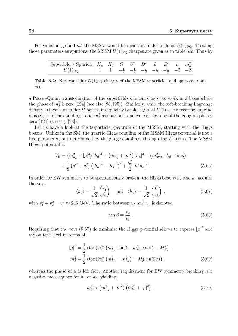
54 5. Supersymmetry
For vanishing µ and m23 the MSSM would be invariant under a global U(1)PQ. Treating
those parameters as spurions, the MSSM U(1)PQ charges are given as in table 5.2. Thus by
Superfield / Spurion Hu Hd Q U c Dc L Ec µ m23
U(1)PQ 1 1 −12−1
2−1
2−1
2−1
2−2 −2
Table 5.2: Non vanishing U(1)PQ charges of the MSSM superfields and spurions µ andm3.
a Peccei-Quinn transformation of the superfields one can choose to work in a basis wherethe phase of m2
3 is zero [124] (see also [98,125]). Similarly, while the soft-breaking Lagrangedensity is invariant under R-parity, it explicitly breaks a global U(1)R. By treating gauginomasses, trilinear couplings, and m2
3 as spurions, one can set e.g. one of the gaugino phaseszero [124] (see e.g. [98]).
Let us have a look at the (s)particle spectrum of the MSSM, starting with the Higgsbosons. Unlike in the SM, the quartic Higgs coupling of the MSSM Higgs potential is not afree parameter, but determined by the gauge couplings through the D-terms. The MSSMHiggs potential is
VH =(m2hd
+ |µ|2)|hd|2 +
(m2hu + |µ|2
)|hu|2 +
(m2
3hu · hd + h.c.)
+1
8
(g′2 + g2
2
) (|hu|2 − |hd|2
)2+g2
2
2|h∗uhd|2 . (5.66)
In order for EW symmetry to be spontaneously broken, the Higgs bosons hu and hd acquirethe vevs
〈hd〉 =1√2
(v1
0
)and 〈hu〉 =
1√2
(0v2
), (5.67)
with v21 + v2
2 = v2 ≈ 246 GeV. The ratio between v2 and v1 is denoted
tan β ≡ v2
v1
. (5.68)
Requiring that the vevs (5.67) do minimise the Higgs potential allows to express |µ|2 andm2
3 on tree-level in terms of
|µ|2 =1
2
(tan(2β)
(m2hu tan β −m2
hdcot β
)−M2
Z
),
m23 =
1
2
(tan(2β)
(m2hu −m2
hd
)−M2
Z sin(2β)), (5.69)
whereas the phase of µ is left free. Another requirement for EW symmetry breaking is anegative mass square for hu or hd, yielding
m43 >
(m2hu + |µ|2
) (m2hd
+ |µ|2). (5.70)
5.4 The Minimal Supersymmetric Standard Model 55
With mSUGRA boundary conditions m2hu
= m2hd
at a high scale, the RGEs typically yieldsmall or negative values of m2
huat the EW scale, such that (5.70) is satisfied in what is
known as radiative EW symmetry breaking. Expanding hu and hd around their vevs (seee.g. [125])
hd =1√2
(v1 + s1 + ip1
h−1
)and hu =
1√2
(h+
2
v2 + ss + ip2
)eiξ , (5.71)
where ξ is a relative phase between hd and hu, one obtains mass matrices
Msspp =
(Mss Msp
M †sp Mpp
)and Mh+h− , (5.72)
with
Msp =
(0 m2
3 sin ξm2
3 sin ξ 0
). (5.73)
Minimising the Higgs potential is equivalent to vanishing tadpole coefficients for s1, s2,p1, and p2. In chapter 10 we resort to the one-loop tadpole equations in order to obtainthe one-loop analogue of (5.69). For the tree-level potential the tadpole coefficient of p1
requires a vanishing phase ξ. Therefore, in general on tree-level and in the CP-conservingcase10 where ξ = 0 to all orders in perturbation theory, Msspp is block diagonal and themass eigenstates have well-defined CP quantum numbers(
Hh
)=
(cosα sinα− sinα cosα
)(s1
s2
),(
AG0
)=
(sin βn cos βn− cos βn sin βn
)(p1
p2
),(
H±
G±
)=
(sin βc cos βc− cos βc sin βc
)(h±1h±2
), (5.74)
with h+1 ≡ (h−1 )∗ and equivalently for h−2 . There are two CP even Higgs bosons h, H in the
real MSSM, where conventionally mh < mH . A is an CP odd Higgs boson and G0, G± arethe three Goldstone bosons that give massive Z and W± bosons. Note that on tree-levelthe requirement of vanishing tadpole coefficients yields βn = βc = β. The tree-level Higgsmasses are given by
m2A =
2m23
sin(2β),
m2H± = m2
A +M2W ,
m2h,H =
1
2
(m2A +M2
Z ∓√
(m2A −M2
Z)2
+ 4M2Zm
2A sin2(2β)
). (5.75)
10We will denote the CP-conserving MSSM as real MSSM and the CP-violating MSSM as complex.

56 5. Supersymmetry
In the CP violating case, the three mass eigenstates h1, h2, and h3 are obtained from
h1
h2
h3
= S
s1
s2
p1
p2
, (5.76)
with S a 3×4 matrix satisfying S†S = 14 and mh1 < mh2 < mh3 (see e.g. [123]). The massof the lightest Higgs bosonmh (ormh1) is strongly affected by loop corrections [126]. Precisecalculations of these loop corrections are very elaborate, in chapter 10 a two-loop Higgsmass calculation will be performed with the published software FeynHiggs [125,127–129].
Turning to the sparticles, the mass eigenstates of gauginos and Higgsinos are four neu-tralinos χ0
i from B, W 0, h0u, and h0
d and two charginos χ±i from W±, h+u , and h−d . Their
mixing matrices are given in appendix B. The superpartners of the SM fermions are sixup-type squarks, six down-type squarks, six charged sleptons, and three sneutrinos. Ingeneral they mix to form mass eigenstates, with the 6×6 (3×3) mass and mixing matricesgiven in appendix B as well.
We close this section with three remarks:
Supersymmetric seesaw In order to extend the MSSM by a type-I seesaw mechanismone introduces a left-handed chiral superfield N c as gauge singlet and adds the superpo-tential terms
Wseesaw = YνijHu · LiN cj +
1
2MnijN
ciN
cj . (5.77)
The soft-breaking Lagrange density is extended by
Lsoft ⊃ −ν∗Rim2νijνRj . (5.78)
Supersymmetric threshold corrections The SM is an effective theory of the MSSM.When solving the MSSM RGEs, the MSSM is commonly matched to the SM at a renormal-isation scale chosen to represent an average mass MSUSY of the sparticles. Conventionallyit is set to the geometric mean of the stop quark masses Q ≡ √mt1mt2 , where the loop-corrected result for the light Higgs mass is numerically stable against small changes of therenormalisation scale [130]. The SUSY scale has to be larger than MZ and typical valuesare assumed to be around 1 TeV.
On tree-level, down-type quarks and charged leptons only couple to the Higgs field hd.On one-loop level however, there are also couplings to hu. These loops yield tan β-enhancedthreshold corrections to Yukawa couplings when the MSSM is matched to the SM and thesparticles are intergrated out [131, 132]. Thus, although loop-suppressed, they can havesignificant magnitude for sizeable tan β and are of importance for the prediction of quark-lepton mass ratios [133]. A full calculation of SUSY threshold corrections will be presentedin chapter 10.

5.5 Supersymmetric SU(5) GUTs 57
Charge and colour breaking vacua Besides the Higgs fields hu and hd, the MSSMscalar potential also contains sfermion fields. In principle those fields can obtain non-vanishing vevs as well, thereby breaking SU(3)C and U(1)em spontaneously. The existenceof such dangerous charge and colour breaking (CCB) minima in the scalar potential islinked to the violation of bounds for the soft-breaking trilinear couplings [134,135], e.g.
|Tij|2 ≤(m2Lii
+m2Rjj
+m2hf
+ |µ|2)
(y2i + y2
j ) i 6= j
3y2i i = j
, (5.79)
where mL, mR, and mhf denote the soft-breaking mass parameters of the scalar fieldsassociated with the trilinear coupling T in the basis of diagonal Yukawa matrices.
Additionally, the scalar potential might feature directions in field space which are un-bounded from below (UFB). For the tree-level scalar potential these yield constraints [134]
m2hu +m2
hd+ 2 |µ|2 > 2m2
3 ,
m2hu + |µ|2 +m2
Li>
m43
m2hd
+ |µ|2 −m2Li
,
m2hu +m2
Li> 0 . (5.80)
Note that the first equation is always satisfied when |µ| is calculated from the requirement(5.69) of successful EW symmetry breaking. If any of the CCB or UFB constraints areviolated for a particular MSSM parameter point, the decay rate of our physical vacuuminto the deeper unphysical one can still be so small, that our vacuum’s lifetime exceeds theage of the universe by orders of magnitude. This will be discussed further in chapter 10.Finally we note that the tree-level scalar potential receives radiative corrections and UFBdirections will become bounded from below eventually, thereby turning into CCB vacua.
5.5 Supersymmetric SU(5) GUTs
As shown in figure 5.4, the field content of the MSSM yields an unification of the gaugecouplings at MGUT ≈ 2 · 1016 GeV, where the αi are defined analogous to the QED fine-
structure constant αi ≡ g2i
4πand the one-loop β function coefficients for the gauge couplings
in the MSSM are b1 = 335
, b2 = 1, and b3 = −3 [86, 136]. This motivates the embeddingof the MSSM gauge group into a GUT gauge group like SU(5). Note that the gaugecouplings do not unify entirely, rather at MGUT small differences11 do remain, but thosecan be attributed to threshold effects from heavy GUT-scale particles, such as the SU(3)Coctet O(24), SU(2)L triplet T (24), SU(3)C triplets T (5), T (5), and heavy gauge bosons Xand Y in an SU(5) GUT [137]. In the last line we have already assumed that the fieldcontent of the Georgi-Glashow SU(5) from section 4.1 is accompanied with superpartners
11Conventionally MGUT is defined by the unification α1(MGUT) = α2(MGUT).

58 5. Supersymmetry
α1-1
α2-1
α3-1
10 105 109 1013 1017
10
20
30
40
50
60
R G s c a l e (GeV)
α-
1
α1-1
α2-1
α3-1
10 105 109 1013 1017
10
20
30
40
50
60
R G s c a l e (GeV)
α-
1
Figure 5.4: One-loop RG evolution of the inverse gauge couplings α−1i in the SM (left)
and MSSM (right), assuming a common SUSY scale MSUSY = 103 GeV. The dashed linesindicate MSUSY = 103 GeV and MGUT ≈ 2 · 1016 GeV.
and embedded into superfields. Because MSUSY MGUT we almost never have the needto write SU(5) superfields in scalar and fermion components notation. Thus we use thesame notation for the superfields as introduced for the corresponding non-SUSY SU(5)multiplet, e.g.
F ⊃ Dc, L and T ⊃ Q,U c, Ec . (5.81)
Because of the two Higgs fields in the MSSM, another SU(5) Higgs multiplet H5, trans-forming as 5, is introduced
H5 ⊃ Hu, T(5) and H5 ⊃ Hd, T
(5) . (5.82)
The embedding of the MSSM superfields into SU(5) multiplets, or equivalently the “su-persymmetrisation” of the Georgi-Glashow SU(5) model, is denoted minimal SUSY SU(5)[138]. The superpotential for this model is given by
W = M24TrH224 + λ24TrH3
24 + (µ5 + λH24)H5H5 + Y5T FH5 + ε5Y10T T H5 , (5.83)
where flavour and SU(5) indices have been suppressed. When SU(5) gets broken the colouroctet O(24), SU(2)L triplet T (24), and gauge singlet S(24) obtain masses
mO(24) = mT (24) =15
4λ24V and mS(24) =
3
4λ24V . (5.84)
In addition to the MSSM superpotential, there are also terms coupling matter superfieldsto the colour Higgs triplets
WT =1√2Y5 (Q · L− U cDc) T (5) + 2Y10 (2U cEc −Q ·Q)T (5) , (5.85)
which leads to dangerous dimension five baryon number violating operators [122,139–143](see also [82])
WB =
√2
MT
(Y5Q · L) (Y10Q ·Q) +2√
2
MT
(Y5UcDc) (Y10U
cEc) . (5.86)

5.5 Supersymmetric SU(5) GUTs 59
These operators have to be “dressed” with gluinos, charginos, or neutralinos to become adimension six proton decay operator, as shown in figure 5.5 for an example. The resulting
QQQ
W
T5Q
Q L
dR Q
uR Le∗R
d∗RHu
HdT †5
˜T5
†
Figure 5.5: Examples for dressed LLLL and RRRR contributions to proton decay medi-ated by the colour triplets T5 and T5. Note that flavour indices are suppressed.
dimension six operators are suppressed by 1MSUSYMT
in contrast to the 1M2T
suppression of
non-supersymmetric dimension six proton decay. Thus the lower bound on the protonlifetime yields a heavy lower limit for the triplet mass [82, 143],
MT & 1017 GeV . (5.87)
A SU(5) GUT model with a heavy Higgs triplet mass of this scale suffers from two prob-lems:
Firstly, there is the problem of doublet-triplet splitting. When SU(5) is broken, theµ-term for the Higgs doublets and the mass of the colour triplets are given by
W ⊃(µ5 −
3λ
2V
)Hu ·Hd + (µ5 + λV )T (5)T (5) . (5.88)
Via fine-tuning of λ, a strong hierarchy between doublet and triplet masses can be achieved.In predictive flavour models, however, employing CG factors via higher dimensional Yukawacoupling operators involvingH24, as discussed in section 4.4, will forbid terms like λH24H5H5
due to discrete symmetries and a fine-tuning solution to DTS will be no longer feasible.Besides fine-tuning, the DTS problem can be solved via the missing partner mechanism(MPM) [144]. We review MPM in part IV of this thesis in chapter 9, where we presentour results for combining predictive SUSY SU(5) flavour models with DTS.
Secondly, the contribution of the colour Higgs triplets to the RGEs of the gauge couplingsspoil the successful unification unless MT . 1015 GeV [145]. Giving up the condition ofrenormalisability for the superpotential
W ⊃M24TrH224 + λ24TrH3
24 +a
Mpl
(TrH2
24
)2+
b
Mpl
TrH424 + (µ5 + λH24)H5H5 , (5.89)
the masses ofO(24) and T (24) split which shifts the upper bound forMT to higher values [146]
MT = M0T
(mT (24)
mO(24)
) 52
, (5.90)
where M0T denotes the triplet mass in the renormalisable minimal SU(5). Building non-
renormalisable operators by coupling H24 to Yukawa operators in general allows to fit the

60 5. Supersymmetry
observed quark-lepton mass ratios, at the cost of loosing predictability. In chapter 9 in themain part of this thesis we will discuss how DTS, a sufficiently heavy triplet mass MT , andgauge coupling unification can be achieved in predictive SUSY flavour GUT models.
Finally we note that the constraint MGUT & 1016 GeV from dimension six proton decay(4.31) is satisfied in minimal SUSY SU(5).
PART III
SUSY Flavour GUT models
CHAPTER 6
θ13PMNS≈ θC sin θ23
PMNS from GUTs
Grand Unified Theories offer a promising setting to predict quark - lepton mass ratios. Aswas discussed in 4.4, when down-type quark Yukawa matrix and charged lepton Yukawamatrix are generated from the same set of GUT operators, the resulting entries are linkedand differ only by group theoretical Clebsch-Gordan factors. This connection is not limitedto quark and lepton masses, however, but also links quark and lepton mixing angles. In thischapter we present our results of [1] and discuss simple conditions such that the large valueof θPMNS
13 can be explained from θPMNS13 ≈ θC sin θPMNS
23 in SU(5) GUTs and PS unification.
6.1 A numerical expression for θPMNS13 in terms of θC
After neutrino oscillations were discovered and large θPMNS12 and θPMNS
23 had been established,it was widely assumed θPMNS
13 would be small or vanishing. In many GUT models smallnon-vanishing θPMNS
13 ≈ 3 was predicted, when the Georgi-Jarlskog CG factor 3 (4.28) wasused to correct the minimal SU(5) prediction Ye = Y T
d in the first two families.
In 2011 a surprisingly large θPMNS13 ≈ 8.8±1.0 was measured by T2K, DoubleCHOOZ,
DayaBay, and RENO [46,147]. Following the discovery, it was noted that by replacing theGeorgi-Jarlskog CG factor with the newly proposed alternatives of [83], large θPMNS
13 couldbe obtained [148,149].
θPMNS13 also complied with a very interesting numerical expression in terms of the Cabibbo
angle θC = 13.02 ± 0.04
θPMNS13 ≈ θC√
2≈ 9.2 . (6.1)
In the meantime the lepton mixing angles have been measured with higher precision [62]
θPMNS12 = 33.48 +0.78
−0.75 , θPMNS13 = 8.50 +0.20
−0.21 , and θPMNS23 =
42.3 +3.0
−1.6 (NO)
49.5 +1.5
−2.2 (IO).
(6.2)

6.1 A numerical expression for θPMNS13 in terms of θC 63
With these updated values the lepton mixing angles still amount to a very interestingnumerical agreement of
θPMNS13 ≈ θC sin θPMNS
23 = 8.84 +0.30
−0.44 , (6.3)
in the case of the NO best fit point. Equation (6.1) follows from (6.3) as a special casewhen θPMNS
23 = 45.1 The appearance of θC in relation (6.3) motivates the viewpoint of anunderlying GUT symmetry connecting the quark and lepton sectors.
Note that even before θPMNS13 was measured various different approaches featuring large
values of θPMNS13 existed in the literature. The estimate θPMNS
13 = O(θC) for example can beobtained from charged lepton corrections if one merely assumes the Wolfenstein parameterλ ≈ θC as expansion parameter in the charged lepton mixing matrix in so-called Cabibbohaze [152], or e.g. in [153]. However, in such scenarios θPMNS
13 is not predicted, since itdiffers from λ by an unknown prefactor. In the context of Quark-Lepton Complementary(QLC) θPMNS
12 +θC = 45 [154] the relation θPMNS13 = θC√
2appeared from assuming bimaximal
neutrino mixing and a lepton mixing matrix U(e)L exactly equal to VCKM [155]. The latter
assumption, however, is not expected to hold in realistic GUTs since the mass matricesof quarks and charged leptons cannot be identical, especially regarding the masses of thefirst two families. The GUT scale mass ratio mµ
msin particular is severely different from
one. As mentioned before, non-universal group-theoretical CG factors are required to bringGUT predictions for quark-lepton mass ratios in accordance with observations. But withdifferent singular values of Yd and Ye, it can not be expected that the charged lepton mixingmatrix equals VCKM.
Yu Yd
YemνCondition 1
Condition 2
Conditions 3 & 4
VPMNS
VCKM
GU
Ts
Figure 6.1: In our set-up, the relation θPMNS13 ≈ θC sin θPMNS
23 is obtained by linking thecharged lepton and quark sectors via GUTs, demanding four constraints on the mixingangles and GUT structure, as discussed in the main text.
In contrast, we will not require bimaximal mixing in the neutrino sector nor identicalU
(e)L and VCKM. In the light of the new CG factors available in model building, our strategy
1In 2011, global fits reported large uncertainties for θPMNS23 , e.g. θPMNS
23 = 46.1±3.4 [147] and θPMNS23 =
40.4 with a one sigma confidence interval of [38.6, 45.0] [150]. Also in 2016 there is still potential forhigher precision, with e.g. a one sigma interval of [38.6, 53.7] reported by the NOνA collaboration forθPMNS
23 [151].

64 6. θ13PMNS≈ θC sin θ23
PMNS from GUTs
is to use GUT relations plus additional conditions/constraints on the structure of SU(5)GUTs and Pati-Salam models, as illustrated in figure 6.1, to establish θe12 ≈ θC , whichthen induces θPMNS
13 ≈ θC sin θPMNS23 via a charged lepton correction to the neutrino mixing
matrix. In 6.5 we come back to a comparison between our results and the QLC relation.
In the following sections we discuss in detail four simple conditions to realise θPMNS13 ≈
θC sin θPMNS23 in GUTs. Note that, while these conditions can act as an instruction how to
build predictive flavour GUT models with θPMNS13 ≈ θC sin θPMNS
23 , we do not claim that ourstrategy is the only functioning set-up. For example, while our paper [1] was finalised, [156]appeared, which also discusses strategies for obtaining θPMNS
13 ≈ θC sin θPMNS23 , e.g. from a
shared flavon in the quark and neutrino sector of a flavour model.
6.2 Conditions for mixing angles
In the following, we will assume hierarchical Yu, Yd, and Ye, which implies that the left-mixing angles θuij, θ
dij, and θeij are all comparatively small (i.e., not much larger than the
Cabibbo angle θC) as is typical for GUT flavour models in the flavour basis.
We first revisit the charged lepton corrections (3.31)
sPMNS23 e−iδ
PMNS23 ≈ sν23e
−iδν23 − θe23c
ν23e−iδe
23 , (6.4a)
θPMNS13 e−iδ
PMNS13 ≈ θν13e
−iδν13 − θe13c
ν23e−iδe
13 − θe12e−iδe
12(sν23e−iδν23 − θe
23cν23e−iδe
23) , (6.4b)
sPMNS12 e−iδ
PMNS12 ≈ sν12e
−iδν12 + θe13c
ν12s
ν23e
i(δν23−δe13) − θe
12cν23c
ν12e−iδe
12 , (6.4c)
in leading order of θν13 and (3.32)
θPMNS13 e−iδ
PMNS13 ≈ θν13e
−iδν13 − θe13c
ν23e−iδe
13 − θe12s
PMNS23 e−i(δ
e12+δPMNS
23 ) , (6.5)
in order to find simple conditions for obtaining a predictive GUT scenario with θPMNS13 ≈
θC sin θPMNS23 . Similarly, the CKM angles θCKM
ij can be expressed in terms of quark mixing
angles θuij and θdij by a small angle expansion of VCKM =(U
(u)L
)†U
(d)L [157]
θCKM23 e−iδ
CKM23 ≈ θd23e
−iδd23 − θu23e−iδu23 , (6.6a)
θCKM13 e−iδ
CKM13 ≈ θd13e
−iδd13 − θu13e−iδu13 − θu12e
−iδu12(θd23e−iδd23 − θu23e
−iδu23) , (6.6b)
θCKM12 e−iδ
CKM12 ≈ θd12e
−iδd12 − θu12e−iδu12 . (6.6c)
The standard PDG Dirac CP phase δCKM in VCKM can be identified as [17]
δCKM = δCKM13 − δCKM
23 − δCKM12 . (6.7)
We are now ready to state first conditions towards scenarios featuring (6.3):

6.3 Conditions from relations between Yd and Ye 65
Condition 1: Since we want to use the charged lepton correction proportional to θe12
to establish the link to θC via GUTs we require, as assumed to derive (3.31) and (3.32),hierarchical Yu, Yd, and Ye, and furthermore
θν13 ≈ 0 , θe13 ≈ 0 . (6.8)
Then the first two summands on the right side of (3.32) drop out and we obtain (3.33),independently of any phases
θPMNS13 ≈ θe
12sPMNS23 . (6.9)
Condition 2: Secondly, since we want to establish a link between θPMNS13 and θC based
on GUT relations between Yd and Ye, we require that to a good approximation
θd12 ≈ θC . (6.10)
This may follow from (6.6c) as a consequence of θu12 θd12, which is a typical feature ofmodels with hierarchical Yukawa matrices where the stronger hierarchy in the up-quarksector implies the smaller mixing angles. An alternative possibility arises when one requiresθu13, θd13 ≈ 0. Such cases yield the quark mixing sum rule [157] from (6.6) and (6.7)
θd12 ≈∣∣∣∣θCKM
12 − θCKM13
θCKM23
e−iδCKM
∣∣∣∣ ≈ 12.0 ± 0.3 . (6.11)
6.3 Conditions from relations between Yd and Ye
To arrive at θPMNS13 ≈ θC sin θPMNS
23 , we want to employ GUT relations between the down-type quark Yukawa matrix Yd and the charged lepton Yukawa matrix Ye. The GUTrelations emerge since the down-type quark Yukawa matrix and the charged lepton Yukawamatrix are generated from joint GUT operators, as discussed in chapter 4. This leads tothe following condition:
Condition 3: To obtain predictive GUT relations, we require that all elements of theYukawa matrices Yd and Ye are each dominantly generated by one single joint GUT oper-ator. This condition can be somewhat relaxed in specific cases, for instance it would besufficient to restrict this requirement to the distinct matrix elements which enter the rela-tion between θC and θe12. Furthermore it is possible that two operators featuring the sameCG factor contribute at similar strength. In this case, the relation between the elements ofYd and Ye is still given by only one single CG factor. We demand the stronger requirementstated at the beginning at this point, to keep the discussion simple.

66 6. θ13PMNS≈ θC sin θ23
PMNS from GUTs
Thus, the matrix elements are closely linked by group theoretical CG factors. For hier-archic Yd and Ye and small mixing angles we can focus our discussion exclusively on the1-2 submatrix of the first two families
Yd =
(d ba c
)⇒
Ye =
(cd d cb b
ca a cc c
)(PS) ,
Ye =
(cd d ca a
cb b cc c
)(SU(5) GUTs)
. (6.12)
Here, ca, cb, cc, and cd are the CG factors relating the elements of Yd and Ye. As discussedin chapter 4, in SU(5) GUTs Yd is related to Y T
e , whereas in Pati-Salam unified theoriesYd is related directly to Ye. Lists of available CG factors in SU(5) and PS were given in(4.45) and (4.46), respectively.
The CG factors play an important role in flavour model building: A successful modelrequires a consistent set of CG factors in (6.12), leading to viable mass relations for thefirst two families. It has been noted in [148,149], that various combinations of phenomeno-logically viable CG factors exist which can lead to a comparatively large θPMNS
13 . Theprediction θPMNS
13 ≈ θC sin θPMNS23 only emerges from a subset of these combinations of CG
factors, as we now discuss in the context of Pati-Salam unified theories and SU(5) GUTs.To obtain conditions on the CG factors, we first note that the 1-2 mixing angle of Yd is
given in leading order in a small mixing approximation by
θd12 ≈∣∣∣∣bc∣∣∣∣ , (6.13)
and the Yukawa couplings by
yd ≈∣∣∣∣d− a b
c
∣∣∣∣ and ys ≈ |c| . (6.14)
6.3.1 θPMNS13 ≈ θC sin θPMNS
23 in Pati-Salam Theories
In Pati-Salam unified theories, to leading order in a small angle approximation the Yukawacouplings ye and yµ of the first two families are given by [148]
ye ≈∣∣∣∣cdd− ca a cb b
cc c
∣∣∣∣ and yµ ≈ |ccc| , (6.15)
and the 1-2 mixing angle θe12 is given by
θe12 ≈∣∣∣∣cb bcc c
∣∣∣∣ ≈ ∣∣∣∣cbcc∣∣∣∣ θC , (6.16)
where (6.10) and (6.13) were used in the last step. Finally, using (6.9) we obtain
θPMNS13 ≈ θe12 sin θPMNS
23 ≈∣∣∣∣cbcc∣∣∣∣ θC sin θPMNS
23 . (6.17)
From here we can read off the condition on the CG factors in Pati-Salam theories:

6.3 Conditions from relations between Yd and Ye 67
Condition 4 (PS): In Pati-Salam unified models, and in general in unified models witha direct GUT relation between Yd and Ye (and not as in SU(5) GUTs between Yd and Y T
e )we require that the CG factors for the operators generating the 2-2 element and the 1-2element of Ye are equal, i.e.
|cb| = |cc| . (6.18)
In Pati-Salam unified theories, this simple additional condition is indeed sufficient andmay readily be implemented in flavour models. The remaining parameters and CG factorsof such a model of course have to be constructed in such a way that the phenomenologicalconstraints on the down-type quark and charged lepton sectors are satisfied. In Pati-Salammodels it turns out that in the case of vanishing 1-1 element d = 0, there is no set of CGfactors available which simultaneously satisfies (6.18) and the double ratio (4.43)∣∣∣∣yµ ydys ye
∣∣∣∣ ≈ ∣∣∣∣ c2c
ca cb
∣∣∣∣ ≈ 10.7+1.8−0.8 . (6.19)
Therefore viable scenarios of Pati-Salam unification require non vanishing 1-1 elements inYd and Ye [148] (see also [158]). Let us remark that in principle the set cc = cb = 9 andca = 3
4yields the double ratio 12, which is also within the one sigma confidence interval,
but the GUT scale relation yµ = 9ys requires SUSY threshold corrections of about 50%,which exceeds typical results in realistic SUSY scenarios (see e.g. [133] and figure 10.3).
We will see next that in SU(5) GUTs zero 1-1 elements of Yd and Ye are consistent andeven favourable for obtaining the relation θPMNS
13 ≈ θC sin θPMNS23 .
6.3.2 θPMNS13 ≈ θC sin θPMNS
23 from SU(5) GUTs
In SU(5) GUTs the 1-2 mixing angle θe12 is given in leading order in a small angle approx-imation by
θe12 ≈∣∣∣∣ca acc c
∣∣∣∣ . (6.20)
Employing (6.13) and condition (6.10) shows that in order to obtain a link between θC andθe12 we need to relate
θC ≈∣∣∣∣bc∣∣∣∣ and θe12 ≈
∣∣∣∣ca acc c∣∣∣∣ (6.21)
This implies that towards establishing a simple link between θPMNS13 and θC in SU(5) GUTs,
we have to impose at least one further constraint on the structure of the Yukawa matrices.From (6.21) one can see that one possibility to restore a direct link between θC and θe12 isto enforce
|a| ≈ |b| (6.22)
which immediately translates into
θe12 ≈∣∣∣∣ca acc c
∣∣∣∣ ≈ ∣∣∣∣cacc∣∣∣∣ θC , (6.23)

68 6. θ13PMNS≈ θC sin θ23
PMNS from GUTs
and thus to a simple condition
|ca| = |cc| ⇒ θPMNS13 ≈ θC sin θPMNS
23 (6.24)
on the CG factors in SU(5) GUTs. We discuss two ways to enforce |a| = |b| (or |a| ≈ |b|to a good approximation) in the following and give two choices for the final condition:
Condition 4.1 (SU(5) GUTs): The first possibility is rather straightforward, namelythat the Yukawa matrices Yd and Ye are symmetric in the 1-2 submatrix considered above.Although this is not a typical feature in SU(5) GUTs, symmetric matrices could be aconsequence of a flavour symmetry in specific models. This would imply that
|a| = |b| and |ca| = |cb| , (6.25)
such that the above condition is satisfied. We note that in order to obtain realistic massratios, in the case of symmetric Yd and Ye, the 1-1 elements have to be non-vanishing andthe CG factor cd has to be chosen appropriately.
Condition 4.2 (SU(5) GUTs): The second possibility is less straightforward but leadsto almost exactly the same prediction. It arises when one imposes vanishing 1-1 elementsof Yd and Ye. Then the resulting structure of the Yukawa matrices is quite predictive, sincethe five observables ye, yµ, yd, ys, and θd12 ≈ θC are determined by only three parameters|a|, |b|, and |c| and the corresponding CG coefficients. In leading order in a small mixingangle approximation, we obtain:
ys ≈ |c| , yµ ≈ |cc c| , yd ≈∣∣∣∣a bc
∣∣∣∣ , ye ≈∣∣∣∣ca a cb bcc c
∣∣∣∣ , θC ≈∣∣∣∣bc∣∣∣∣ . (6.26)
This situation has been considered in [148] and the relation
θe12 ≈yeyµ
∣∣∣∣cccb∣∣∣∣ 1
θC(6.27)
has been derived. There is an interesting phenomenological relation between the Cabibboangle and the quark mass ratio (2.38)
ms
md
= 18.9± 0.8 , (6.28)
commonly known as GST-relation
θC ≈√
1
19≈√ydys. (6.29)
Historically it was first phrased in [159] as θ2C ≈ m2
π
2m2K
, where mπ and mK denote pion
and kaon masses, respectively, and in [160] in the context of quark masses. Necessary

6.4 Corrections to θPMNS13 ≈ θC sin θPMNS
23 69
constraints for (6.29) to hold in viable flavour models are [161] approximately vanishing1-1 element of Yd and |a| ≈ |b|, as can be seen from (6.26)
ydys≈∣∣∣∣a bc2
∣∣∣∣ ≈ ∣∣∣ab ∣∣∣ θ2C . (6.30)
Thus, although less direct than in condition 4.1, |a| ≈ |b| is found via vanishing 1-1 element
of Yd and the GST relation. From (6.23) the connection to θC , i.e. θe12 ≈∣∣∣ cacc ∣∣∣ θC , is obtained,
thus realising θPMNS13 ≈ θC sin θPMNS
23 .Note that cb has to be properly chosen in addition to |ca| = |cc|, to yield viable GUT
scale quark-lepton mass ratios for the first two families [148, 149]. In SU(5) GUTs withzero 1-1 elements in Yd and Ye, only one combination of CG factors listed in (4.45) results inθPMNS
13 ≈ θC sin θPMNS23 , while being consistent with phenomenological constraints (including
msmd≈ 19), namely
cc = ca = 6 , cb = −1
2. (6.31)
6.4 Corrections to θPMNS13 ≈ θC sin θ
PMNS23
As we have discussed above, the relation θPMNS13 ≈ θC sin θPMNS
23 can emerge under foursimple conditions from GUTs, by charged lepton contributions to VPMNS and linking θe12
to θC . Let us now discuss how this relation is affected by certain, unavoidable corrections,for example from RG running between the GUT scale where the prediction arises and lowenergies where the neutrino oscillation experiments are performed. Other corrections arisefrom the fact that we presented leading order results in a small mixing approximation.
Note that given a specific flavour model, the deviation from the exact relation can becalculated, and future more precise measurements of the lepton mixing angles may allowto discriminate between different models realising θPMNS
13 ≈ θC sin θPMNS23 .
Possible corrections are:
Corrections due to small mixing approximation: In 6.3 we omitted higher orderterms in a small mixing angle expansion to keep our discussion as simple as possible. Theerror introduced by this simplification depends on the structure of the Yukawa matricesand on the CG factors and can easily be computed. Let us consider, for instance, theexample of a SU(5) GUT with zero 1-1 elements in Yd and Ye and CG factors as in (6.31),i.e.
Yd =
(0 ba c
), Ye =
(0 6 a−1
2b 6 c
). (6.32)
Instead of a small angle approximation, we numerically perform an exact diagonalisationof the Yukawa matrices (6.32) and find θe12 = 13.8 from a fit to the experimental valuesyeyµ
and θC . The more precise GUT scale prediction is thus
SU(5) with d = 0, cc = ca = 6, cb = −12, and θd
12 = θC : θPMNS13 ≈ 9.3 . (6.33)

70 6. θ13PMNS≈ θC sin θ23
PMNS from GUTs
Corrections from θd12 6= θC: In explicit flavour GUT models, condition 2 may not beexactly fulfilled. Without a specific model, this is a source of theoretical uncertainty.Within a specific model, however, such a deviation is calculable and results in a modifiedprediction for θPMNS
13 , which may open up the possibility to distinguish explicit flavourmodels with a future more precise measurement of the lepton mixing angles. As mentionedabove, the quark mixing sum rule (6.11) yields θd12 ≈ 12.0 ± 0.3 6= θC in models whereθu13, θd13 ≈ 0.
Let us study this in more detail in a Pati-Salam model with CG factors 9 and −3,where we assume embedding in a SO(10) GUT or a suitable flavour symmetry, such thatthe Yukawa matrices are symmetric, i.e.
Yd =
(d bb c
), Ye =
(9 d −3 b−3 b −3 c
). (6.34)
As above, we perform an exact diagonalisation of the Yukawa matrices and fit to theexperimental value of ye
yµand θd12 = 12.0. We obtain the prediction
PS with θu13 ≈ θd13 ≈ 0, a = b, cd = 9, and cb = cc = −3: θPMNS13 ≈ 8.2 . (6.35)
Corrections due the uncertainty of θPMNS23 : There is still a large uncertainty for the
value of θPMNS23 . The most immediate uncertainty is caused by the dependence of θPMNS
23
on the yet undetermined mass ordering of neutrinos. But even when a specific ordering isassumed as prior, the relative uncertainty induced in the prediction for θPMNS
13 still amountsto about 5% (3%) for normal (inverse) mass ordering. Note that [62] reports a 3σ rangefor θPMNS
23 of [38.3, 53.3] in the general case where no specific mass ordering is assumed.As mentioned above, the NOνA experiments finds an one sigma interval of [38.6, 53.7]for θPMNS
23 [151]. An improved experimental accuracy for θPMNS23 and a measurement of the
neutrino mass ordering are therefore necessary in order to predict θPMNS13 more precisely.
Corrections due to RG evolution: Let us now discuss the impact of RG corrections.The relation θPMNS
13 ≈ θC sin θPMNS23 is defined at the GUT scale. Our strategy is to run the
measured values of θC and θPMNS23 up to MGUT to determine θPMNS
13
∣∣MGUT
, and then perform
the RG running of θPMNS13 |MGUT
down to the electroweak scale MEW to obtain θPMNS13
∣∣MEW
,the parameter measurable in experiments. For simplicity, we assume a strongly hierarchicalneutrino mass spectrum with m1 = 0 (NO) or m3 = 0 (IO) in the MSSM. The running ofθC is known to be tiny (see e.g. [91]) and will be neglected in the following.
Using the analytical results of [162], one can estimate
∆sPMNS23 ≡ sPMNS
23
∣∣MEW
− sPMNS23
∣∣MGUT
(6.36)
6.4 Corrections to θPMNS13 ≈ θC sin θPMNS
23 71
in leading logarithmic approximation and in leading (zeroth) order in θPMNS13 :
∆sPMNS23 ≈
(ySMτ )2(1 + tan2 β)
16π2ln
(MGUT
MEW
)(cPMNS
23 )2sPMNS23 (NO) ,
−(ySMτ )2(1 + tan2 β)
16π2ln
(MGUT
MEW
)(cPMNS
23 )2sPMNS23 (IO)
. (6.37)
For the running of θPMNS13 , we obtain for
∆θPMNS13 ≡ θPMNS
13
∣∣MEW
− θPMNS13
∣∣MGUT
(6.38)
in leading (first) order in θPMNS13 :
∆θPMNS13 ≈
(ySMτ )2(1 + tan2 β)
16π2ln
(MGUT
MEW
)(
2m2
m3
cos(δPMNS + αPMNS1 − αPMNS
2 )cPMNS12 sPMNS
12 cPMNS23 sPMNS
23 (NO)
+ (cPMNS23 )2θPMNS
13
),
−(ySMτ )2(1 + tan2 β)
16π2ln
(MGUT
MEW
)(cPMNS
23 )2θPMNS13 (IO) ,
(6.39)where αPMNS
1 and αPMNS2 denote the Majorana phases introduced in (3.16). θPMNS
13
∣∣MEW
can
now be predicted in terms of the measured values of θC and θPMNS23
∣∣MEW
using the GUT
scale relation (6.3):
θPMNS13
∣∣MEW
= θC sPMNS23
∣∣MGUT
+ ∆θPMNS13
= θC
(sPMNS
23
∣∣MEW
−∆sPMNS23
)+ ∆θPMNS
13 . (6.40)
Remarkably, in the case of an inverse mass ordering the terms ∆θPMNS13 and θC ∆sPMNS
23
cancel each other at leading order, while for normal ordering only the term proportionalto the neutrino mass ratio m2
m3remains. Plugging in the experimental values of the mixing
parameters and ySMτ ≈ 0.01 we obtain the following estimate for the effects of RG running:
θPMNS13
∣∣MEW
≈
θC sPMNS
23
∣∣MEW
+ 0.2 cos(δPMNS + αPMNS
1 − αPMNS2
)(tan β
50
)2
(NO) ,
θC sPMNS23
∣∣MEW
(IO) .
(6.41)In the IO case corrections coming from the next order terms are estimated to be about
O(0.05)(
tanβ50
)2. It is thus in general a rather good approximation to evaluate (6.3) with

72 6. θ13PMNS≈ θC sin θ23
PMNS from GUTs
the measured parameters at low energies, even more so for the case of an inverse massordering, where the effects due to RG evolution are negligible small.
Note that the above treatment does not include running of neutrino Yukawa couplingsin type-I seesaw scenarios. Such effects contribute above the mass thresholds of heavyright-handed neutrinos. They are more model dependent and can be estimated using theanalytical formulae of [163] or calculated numerically, e.g. using the Mathematica packageREAP [163]. For hierarchical neutrino Yukawa matrices dominated by a large 3-3 elementYν33 one can obtain an estimate for the additional correction by simply replacing(
ySMτ
)2(1 + tan2 β) ln
MGUT
MEW
−→ Y 2ν33
lnMGUT
Mr3
(6.42)
in the above equations, where Mr3 is the mass of the corresponding righthanded neutrino.Let us remark that when matching the MSSM to the SM at MSUSY, effects from SUSY
threshold corrections on θC and the lepton mixing angles are negligible to a very goodapproximation. A numerical calculation can be performed with SusyTC [5], which will bepresented in chapter 10.
Corrections from canonical normalisation: Finally there can be corrections fromcanonical normalisation of kinetic terms from a non-trivial Kahler metric, as it emergese.g. by integrating out heavy messenger fields in a flavour model, as discussed below (5.47).Since the effective Kahler potential in such scenarios contains terms proportional to theYukawa couplings, it is typically dominated by third family effects. For example, in aspecific flavour GUT model the effective Kahler metric might be written in leading orderas e.g. [107,108]
K ≈ k0
(1+
k3
k0
〈φ†3〉〈φ3〉M2
3
), (6.43)
where k0 and k3 are order one coefficients and φ3 is a heavy messenger field of mass M3
yielding third family Yukawa couplings of y3 ≈ 〈φ3〉M3
. Then, defining
ηCN ≡ k3
k0
〈φ†3〉〈φ3〉M2
3
(6.44)
results in formulae analogous to the case of the RG corrections discussed above as estimatefor the CN corrections [107, 108]. This formulae are given by (6.37) and (6.39) upon thereplacement (
ySMτ
)2(1 + tan2 β) ln
MGUT
MEW
−→ 8π2ηCN . (6.45)
Thus, in scenarios with an inverse mass ordering the relation θPMNS13 ≈ θC sin θPMNS
23 is alsoquite insensitive to CN corrections.
Note that while (6.45) holds in general in theories with dominant third family contri-butions to K, the specific form for ηCN (6.43) and (6.44), and whether or not ηCN is ofsignificant magnitude, are highly model dependent. Whereas in some models the effect
6.5 The underlying neutrino mixing pattern in the light ofθPMNS
13 ≈ θC sin θPMNS23 73
of CN corrections can be of the same size as RG running corrections (in the NO case) orlarger, there are classes of models where CN effects are negligibly small (cf. [107]).
To summarise, in general the uncertainties for the relation θPMNS13 ≈ θC sin θPMNS
23 canamount up to about O(10%), which is larger than the current experimental uncertainty.However, it is important to note that within an explicit flavour GUT model, these cor-rections can be explicitly calculated, thereby decreasing the uncertainty drastically. Witha typical theoretical uncertainty for θPMNS
13 of roughly ±0.25 in a careful model analysis,it is thus possible to discriminate between specific flavour GUT models. In the followingtwo chapters two predictive flavour GUT models featuring θPMNS
13 ≈ θC sin θPMNS23 will be
constructed and analysed.
6.5 The underlying neutrino mixing pattern in the
light of θPMNS13 ≈ θC sin θ
PMNS23
Assuming hierarchic Yukawa matrices such that condition 1 (θν13, θe13 θC) and θe23 θCare satisfied, the mixing angle θν12 is related to θPMNS
13 and θPMNS12 by the lepton mixing sum
rule2 (3.34) [65–67]
sν12 ≈ sPMNS12 − θPMNS
13 cPMNS12 cot θPMNS
23 cos δPMNS , (6.46)
which in the light of θPMNS13 ≈ θC sin θPMNS
23 becomes
sν12 ≈ sPMNS12 − θC cPMNS
23 cPMNS12 cos δPMNS . (6.47)
Thus, based on a specific model for neutrino mixing, the Dirac CP phase δPMNS can bepredicted.
For example, if bimaximal mixing is realised in the neutrino sector, i.e. θν12 = 45, thelepton mixing sum rule becomes
θPMNS12 − θC cPMNS
23 cos(δPMNS
)≈ 45 . (6.48)
Note that this differs substantially from the QLC relation θC + θPMNS12 = 45. With the
experimental data for the mixing angles, (6.48) predicts a Dirac CP phase δPMNS ≈ 180.As a further example, let us consider tri-bimaximal neutrino mixing, i.e. sin(θν12) = 1√
3,
such that the lepton mixing sum rule is given by
θPMNS12 − θC cPMNS
23 cos(δPMNS
)≈ arcsin
(1√3
). (6.49)
Then one predicts a Dirac CP phase of
δPMNS = 100.8 +4.6
−4.7 . (6.50)
2RG corrections to the lepton mixing sum rule have been discussed in [164].

74 6. θ13PMNS≈ θC sin θ23
PMNS from GUTs
Note that such values for δPMNS at the EW scale can result from specific GUT scalepredictions for δPMNS ∈ 0,±90, 180 in explicit flavour GUT models with discreteshaping symmetries like Z2 or Z4 in the context of spontaneous CP violation (see e.g. [165]and the flavour GUT models in the following chapters).
Finally, let us emphasise again that we do not require tri-bimaximal or bimaximalneutrino mixing to obtain the prediction θPMNS
13 ≈ θC sin θPMNS23 from GUTs. The only
requirement on the neutrino sector is θν13 θC in condition 1. The future long baselineneutrino oscillation experiment DUNE [69] aims to measure δPMNS and the lepton mixingsum rule can be understood to “reconstruct” the value of θν12 via a future measurement ofthe Dirac CP phase, as shown in figure 6.2. Thus, using the lepton mixing sum rule (6.47),a precise measurement of θPMNS
12 , θPMNS13 , and δPMNS may hint at a specific neutrino mixing
pattern.
0o 45o 90o 135o 180o-45o-90o-135o-180o
25o
30o
35o
40o
45o
δPMNS
θ12ν
Figure 6.2: One sigma hpd intervals from a Monte Carlo simulation of the lepton mixingsum rule (6.47) in case of normal (blue) and inverse (red) neutrino mass ordering. Ameasurement of δPMNS allows to determine θν12 (under the conditions θν13, θe13, θe23 θC).See appendix C for a definition of hpd intervals.

CHAPTER 7
A SUSY flavour GUT model with
θ13PMNS≈ θC sin θ23
PMNS
In this chapter we propose a predictive supersymmetric SU(5) GUT model with an A4
flavour symmetry, supplemented by discrete shaping symmetries and an R-symmetry,which realises the relation (6.3)
θPMNS13 ≈ θC sin θPMNS
23 , (7.1)
based on [2]. The neutrino sector features tri-bimaximal mixing, and (6.3) emerges fromthe charged lepton contribution to the lepton mixing matrix, which in turn is linked toquark mixing via specific GUT relations, as discussed in the previous chapter. In additionto θPMNS
13 , the model leads to promising quark lepton mass ratios in excellent agreementwith experimental results. Our model also features spontaneous CP violation, with allquark and lepton CP phases determined from flavour symmetry breaking.
7.1 Outline of the model
Our model is constructed with the requirement to satisfy the four conditions of the previouschapter. In this section we discuss how they are implemented in our model. The desiredstructure of the Yukawa matrices will be achieved, as we discuss in the next section, viaspontaneously breaking the flavour symmetry A4 by vevs of flavon fields, which – due toan appropriate potential for the flavons – point in specific directions of flavour space.
Condition 1: θe13, θν13 ≈ 0 will be satisfied by constructing a Yukawa matrix Ye withvanishing 1-3 element and tri-bimaximal mixing in the neutrino sector.
Condition 2: θd12 ≈ θC is achieved by constructing Yd and Yu with vanishing 1-3 elements,such that the quark mixing sum rule (6.11) is realised. Additionally, under the condition

76 7. A SUSY flavour GUT model with θ13PMNS≈ θC sin θ23
PMNS
θu13, θd13 ≈ 0, the quark unitarity triangle angle
α ≡ arg
(− VtdV
∗tb
VudV ∗ub
)= arg
(−(s23s12 − c23s13c12e
iδ)c23c13
c12c13s13eiδ
)
≈ arg
(1− θ23θ12
θ13
e−iδ), (7.2)
where the subscript CKM was suppressed for higher readability, is given by a phase sumrule [157]
α ≈ arg
(θd12
θu12
ei(δd12−δu12)
)= δd12 − δu12 . (7.3)
Equations (6.6) and (6.7) were used to derive (7.3) from (7.2). Thus, a right-angled quarkunitarity triangle with α ≈ 90 can be achieved by constructing Yd with purely imagi-nary 1-2 element and Yu with purely real 1-2 element, yielding δd12 = 90 and δu12 = 0,respectively, when all other elements in the 1-2 submatrices are real. There are two moreexpressions that can be obtained from (6.6) and (6.7) with θu13, θd13 ≈ 0 [157]
θu12 ≈θCKM
13
θCKM23
,θCKM
13 θCKM12
θCKM23
e−iδCKM ≈ −θu12
(θd12e
−i(δd12−δu12) − θu12
). (7.4)
From (6.11) and (7.4), the experimental value δCKM = 71.1 ± 3.1 yields
δd12 − δu12 = 86.1 ± 3.3 . (7.5)
Note that the experimental value of α is given by α = 85.4 +3.9
−3.8 . Thus our set-up impliesa realistic value for δCKM, by a single purely imaginary 2-2 entry in Yd.
Due to the SU(5) relation the 2-2 element of Ye is purely imaginary as well, and theCP violation is carried from the quark to the lepton mixing sector, yielding a Dirac CPphase δPMNS ≈ 90. Thus, from the discussion in 6.5 and the lepton mixing sum rule(6.47), the neutrino sector must feature tri-bimaximal mixing. In our model we thereforeemploy type-I seesaw and Constrained Sequential Dominance (3.43), as described in 3.3.Our model will also include a charged lepton mixing θe23, which can generate a deviationof θPMNS
23 from maximal mixing.Note that the feature of purely imaginary Yukawa matrix elements can be achieved
by a suitable flavon alignment potential as well, such that CP symmetry is broken onlyspontaneously due to CP-violating vevs of flavon fields.
Condition 3: All relevant elements of Ye and Yd will be generated by single GUT-operators in order to construct predictive quark-lepton relations.
Condition 4: In the setting of an SU(5) GUT, we construct Yd and Ye with vanishing1-1 elements. As mentioned in the previous chapter, we therefore must use GUT operators

7.2 The model 77
that yield the CG factors c12 = 6, c21 = −12, and c22 = 6 (where cij is the CG factor of the
i-j element of Ye).Note that, since the CG factors play a crucial role for the phenomenological viability of
the model, it is essential that we not only provide an effective model at the GUT scale, butthat we also specify the messenger sector, which when integrated out realises only singleGUT operators with predictive CG factors, as discussed in 4.4.
We pursue the following procedure to construct a model with the features describedabove:
• In our model the rows respectively columns of the Yukawa matrices are generated asvevs of flavon fields, which are triplets of the flavour symmetry group A4.
In order to obtain the desired structure of the Yukawa matrices, we first find a suitableset of effective operators for the matter sector, appropriate vevs for the flavon fields anda viable alignment potential generating these vevs.
• The next step is to identify the shaping symmetry of the thus specified superpotential.As shaping symmetry we denote Zn and U(1) symmetries, required in addition to A4,to forbid terms which would spoil the desired features. Note that, since one can al-ways redefine several Zn symmetries by linear combinations into another set of Zns, theresulting shaping symmetry is not unique.
• Now we turn to the UV completion of the effective superpotential and find a suitableset of messenger fields, that, when integrated out, can generate all effective operators.Usually, one has a sizeable freedom of choice in doing so, both from using different rep-resentations for the messengers and from using different “topologies” for the supergraphdiagrams. An important constraint on the messenger sector is, however, that it mustguarantee the correct CG factors for the effective operators of Ye, see 4.4.
• Finally, with the flavon, matter, Higgs, and messenger field content at hand, and thegiven shaping symmetry, one has to check whether the most general superpotentialcontains any additional effective operators, which spoil the desired features of the Yukawamatrices. If this is the case, one has to modify some choice made in one of the previoussteps, be it the flavon alignment, the structure of the effective superpotential or the setof messenger fields. Ultimately, a consistent flavour model is developed, by successivelygoing through the previous steps and gradually improving the different sectors, until nosuch dangerous operators are present.
7.2 The model
We now present our model in detail. The matter content of SUSY SU(5) is embeddedinto one A4 triplet F , which thus contains all three families Dc
i and Li, and into threeA4-invariant singlets Ti, one for each family. Additionally, we introduce two right-handedneutrinos N c
1 and N c2 as invariant singlets under A4 and SU(5). The Higgs sector contains
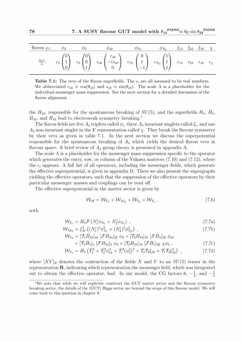
78 7. A SUSY flavour GUT model with θ13PMNS≈ θC sin θ23
PMNS
flavon ϕi: φ2 φ3 φab φN1 φN2 ξ12 ξ23 ξM χ
〈ϕi〉Λ
: ε2
010
ε3
001
εab
cab−isab
0
εN1
01−1
εN2
111
ε12 ε23 εM εχ
Table 7.1: The vevs of the flavon superfields. The εi are all assumed to be real numbers.We abbreviated cab ≡ cos(θab) and sab ≡ sin(θab). The scale Λ is a placeholder for theindividual messenger mass suppression. See the next section for a detailed discussion of theflavon alignment.
the H24, responsible for the spontaneous breaking of SU(5), and the superfields H5, H5,H45, and H45 lead to electroweak symmetry breaking.1
The flavon fields are fiveA4 triplets called φi, threeA4 invariant singlets called ξi, and oneA4 non-invariant singlet in the 1′ representation called χ. They break the flavour symmetryby their vevs as given in table 7.1. In the next section we discuss the superpotentialresponsible for the spontaneous breaking of A4 which yields the desired flavon vevs inflavour space. A brief review of A4 group theory is presented in appendix A.
The scale Λ is a placeholder for the messenger mass suppression specific to the operatorwhich generates the entry, row, or column of the Yukawa matrices (7.10) and (7.12), wherethe εi appears. A full list of all operators, including the messenger fields, which generatethe effective superpotential, is given in appendix D. There we also present the supergraphsyielding the effective operators, such that the suppression of the effective operators by theirparticular messenger masses and couplings can be read off.
The effective superpotential in the matter sector is given by
Weff =WYν +WMR+WYd +WYu , (7.6)
with
WYν = H5F (N c1φN1 +N c
2φN2) , (7.7a)
WMR= ξ2
M
((N c
1)2φ2N1
+ (N c2)2φ2
N2
), (7.7b)
WYd = [T1H45]45 [FH24]45 φ2 + [T2H24]10 [FH5]10 φab
+ [T3H5]5 [FH24]5 φ3 + [T3H24]10 [FH5]10 χφ2 , (7.7c)
WYu = H5
(T 2
3 + T 22 φ
2ab + T 2
1 (φ22)2 + T2T3ξ23 + T1T2ξ
512
), (7.7d)
where [XY ]R denotes the contraction of the fields X and Y to an SU(5) tensor in therepresentation R, indicating which representation the messenger field, which was integratedout to obtain the effective operator, had. In our model, the CG factors 6, −1
2, and −3
2
1We note that while we will explicitly construct the GUT matter sector and the flavour symmetrybreaking sector, the details of the (GUT) Higgs sector are beyond the scope of this flavour model. We willcome back to this question in chapter 9.

7.2 The model 79
arise from contractions mediated by messengers transforming as 10, 45, and 5 underSU(5), coupling to H5 and H45, respectively, as can be seen in table 4.1. Since we needthese specific contractions for our model to work, it is essential that we also construct themessenger sector. The full set of messenger fields, together with their charges, is shown inappendix D.
Note that for the sake of brevity, we do not explicitly write down the appropriatesuppression by powers of the relevant mass scales Λ (which are different for each operator)in (7.7), and we also suppress the couplings in front of each term.
In order to parametrise the resulting Yukawa matrices, we define the quantities
εi ≡〈H24〉
Λεi and εχ ≡
〈H24〉〈φ2〉Λ2
εχ, (7.8)
where again Λ is a placeholder for the individual messenger mass.After GUT and flavour symmetry breaking, the superpotential for the Yukawa matrices
and right-handed neutrino mass matrix (5.64) and (5.77) is given by
W = YeijHd · LiEcj + YdijHd ·QiD
cj − YuijHu ·QiU
cj + YνijHu · LiN c
j +1
2MnijN
ciN
cj , (7.9)
with the Yukawa matrices of the quarks and charged leptons given by
Yd =
0 ε2 0εabcab −iεabsab 0
0 ωεχ ε3
, Ye =
0 6εabcab 0−1
2ε2 −i6εabsab 6ωεχ
0 0 −32ε3
, Yu =
ε42 ε512 0ε512 ε2ab ε23
0 ε23 yt
,
(7.10)up to subleading corrections from higher-dimensional operators or canonical normalisation.With the messenger sector of the model specified in appendix D both corrections can beneglected. The rows and columns of the down-type quark and charged lepton Yukawamatrices, respectively, are built from flavon vevs. The phase
ω ≡ e2πi3 (7.11)
comes from the fact that the flavon field χ transforms as one-dimensional 1′ representationof A4. The hierarchy in Yu is generated by the different powers of flavon vevs in each entry.
The neutrino Yukawa matrix respectively the mass matrix of the heavy neutrinos aregiven by (3.43)
Yν =
0 εN2
εN1 εN2
−εN1 εN2
, MR =
(MR1 0
0 MR2
). (7.12)
The mass matrix of the light neutrinos is obtained from the type-I seesaw formula (3.7)
mν = −v2u
2
A A AA A+B A−BA A−B A+B
, with A ≡ ε2N2
MR2
, B ≡ ε2N1
MR1
, (7.13)
which implies tri-bimaximal mixing in the neutrino sector. Note that, since mν dependsonly on the two parameters A and B, we are free to fix two of the four parameters whichenter Yν and MR, as discussed below in (7.27).

80 7. A SUSY flavour GUT model with θ13PMNS≈ θC sin θ23
PMNS
7.3 Flavon alignment
Here we present the mechanism responsible for the vacuum alignment of the A4-tripletflavons φi, the A4-invariant flavons ξi, and the flavon χ in the 1′ representation of A4. Fora brief review of A4 group theory, see appendix A.
The scalar potential for the flavon fields is obtained from the F -term contributions ofthe driving fields Si, Di, Ai, and Oi, which have U(1)R charge 2. Under the A4 flavoursymmetry they transform as singlets, with the exception of A, D′, and D′′, which transformas 3, 1′, and 1′′, respectively. In the supersymmetric vacuum the F -terms are required tovanish, which forces the scalar components of the flavon fields to obtain the desired vevs.All flavons and driving fields are listed in the lower part of table D.1 in the appendix,together with their charges under the imposed symmetries. Note that the S-fields areall singlets with respect to all symmetries (apart from U(1)R symmetry) and hence areinterchangeable.
After the messenger fields are integrated out, the effective superpotential responsible forthe vacuum alignment of the flavon field vevs, as listed in table 7.1, is given by
Wflavon =W⊥ +WN1N2 +Wab +Wχ +WM +W12 , (7.14)
with2
W⊥ = S2
((φ2
2)3 −M22
)+ S3
(φ2
3 −M23
)+ A2(φ2 ? φ2) + A3(φ3 ? φ3) +O2;3(φ2φ3) , (7.15a)
WN1N2 = SN1
((φN1 ? φN1)2φ2
N1−M2
N1
)+DN1(φN1 ? φN1)φN1 +ON1;N2(φN1φN2)
+ SN2
((φ2
N2)3 −M2
N2
)+D′N2
(φ2N2
)1′′ +D′′N2(φ2
N2)1′ , (7.15b)
Wab = Sab((φab ? φab)
2ξ223 −M2
ab
)+Dα
ab
(φ2ab + λab ξ
223
)+Dβ
ab(φab ? φab)φab
+Dγab
((φ2
ab)1′(φ2ab)1′′ + kab (φab ? φab)
2), (7.15c)
Wχ = Sχ(χ6 −M2
χ
), (7.15d)
WM = SM(ξ6M −M2
M
), (7.15e)
W12 = S12
(ξ6
12 −M212
), (7.15f)
where “?” denotes the symmetric product of two A4 triplets (see appendix A) and thebrackets (. . . )1′ and (. . . )1′′ indicate that the fields are contracted to the 1′ and 1′′ repre-sentation of A4, respectively.
The constants M2 are real due to invariance under CP symmetry.3 Then the terms ofthe type
S(ϕn −M2) (7.16)
2As we did for the matter superpotential, we omit the appropriate suppressions by powers of themessenger masses.
3Note that we checked the CP invariance of our superpotentials using the generalised CP transformationapplicable to models with the discrete flavour group A4 [166]. See appendix A for a brief review.

7.3 Flavon alignment 81
restrict the phases of the flavon vevs to specific discrete values. In particular, among thediscrete vacua for the phases there are the possibilities of 0 and 180 for n even andM2 > 0, which we assume everywhere in (7.15). Thus it is possible to obtain the desiredpurely imaginary 2-2 elements in Ye and Yd and CP is broken spontaneously by the vev ofφab. The real vevs of χ, ξM , and ξ12 are then obtained, up to a discrete choice, as in table7.1. Let us discuss the alignment of the remaining flavon fields in detail.
W⊥: Denoting the components of the triplets φ2 and φ3 with x1, x2, x3, and y1, y2, y3,respectively, the terms containing the triplet driving fields, e.g.
A2 (φ2 ? φ2) = A2
x2x3
x3x1
x1x2
, (7.17)
force two of each 〈φi〉’s components to vanish. The term containing the A4 singlet
O2;3 (φ2φ3) = O2;3(x1y1 + x2y2 + z3y3) (7.18)
forces 〈φ2〉 and 〈φ3〉 to be orthogonal. The phase and magnitude of the vevs is then fixedby the S terms as discussed above
S2
((x2
1 + x22 + x2
3
)3 −M22
), S3
((y2
1 + y22 + y2
3
)−M2
3
), (7.19)
such that W⊥ has a supersymmetric minimum at the points 〈φ2〉 and 〈φ3〉 specified intable 7.1.
WN1N2: The vev 〈φN2〉 is fixed by the second line of WN1N2 . The two terms
D′N2(φ2
N2)1′′ +D′′N2
(φ2N2
)1′ = D′N2
(x2
1 + ωx22 + ω2x2
3
)+D′′N2
(x2
1 + ω2x22 + ωx2
3
)(7.20)
force x21 = x2
2 = x23, and the SN2 term again fixes phase and magnitude such that 〈φN2〉 ∝
(1, 1, 1)T . The vev 〈φN1〉 is constrained by
DN1(φN1 ? φN1)φN1 = 3 DN1y1y2y3 , (7.21)
which requires the vanishing of one component, and the orthogonality condition between〈φN1〉 and 〈φN2〉, which results from setting the F -term of ON1;N2 to zero. Then, with phaseand magnitude set by the F -term of SN1 , one obtains 〈φN1〉 ∝ (0, 1,−1)T as in table 7.1.
Wab: Here, the S-term determines the magnitude and the overall phase of the product〈φab〉〈ξ23〉. The individual magnitudes and the relative phase between 〈φab〉 and 〈ξ23〉 aredetermined by
Dαab
(φ2ab + λab ξ
223
). (7.22)
One of the components of 〈φab〉 is required to vanish by the term with the driving fieldDβab, analogously to (7.21). With the overall phase and norm of 〈φab〉 fixed, the relative

82 7. A SUSY flavour GUT model with θ13PMNS≈ θC sin θ23
PMNS
magnitude tan θab ≡∣∣ab
∣∣ and phase ϕ of the two non-vanishing components a and b areconstrained by
Dγab
((φ2
ab)1′(φ2ab)1′′ + kab (φab ? φab)
2)
= Dγab
(a4 + b4 + (kab − 1)a2b2
). (7.23)
Setting the F -term of Dγab to zero, one obtains
a2
b2+b2
a2= (1− kab) . (7.24)
Depending on the value of kab there are three distinct solutions for a and b
−1 ≤ kab ≤ 3 : tan θab = 1 kab = 1− 2 cos(2ϕ)kab < −1 : ϕ ∈ 0, π kab = −1− 4 cot2(2θab)kab > 3 : ϕ = ±π
2kab = 3 + 4 cot2(2θab)
(7.25)
Thus, with an appropriate choice of kab, the potential has a minimum at the points 〈φab〉and 〈ξ23〉 given in table 7.1.
7.4 Phenomenology
In this section we perform a fit of the model’s GUT scale parameters to experimental datagiven at the low energy scale of the MS top mass mt(mt). Towards this end, the RGrunning from MGUT to mt(mt) has to be performed, including SUSY threshold effects atMSUSY where the MSSM is matched to the SM. Here we discuss the numerical procedureof our analysis and present the results.
7.4.1 Numerical procedure
The fit is performed in the following way: Using the one-loop MSSM RGEs of the Math-ematica package REAP [163], we run the parameters in the MSSM from MGUT to a con-jectured SUSY scale MSUSY = 1 TeV. REAP automatically integrates out the heavy, right-handed neutrinos at their respective mass scales and calculates the effective mass matrixof the light neutrinos from the see-saw formula (3.7).
In our analysis we include the tan β-enhanced SUSY threshold corrections at MSUSY inthe basis where Yu is diagonal, with the approximate matching relations given by [132]
Y SMd = (1+ diag(ηQ12 , ηQ12 , ηQ3)) Y MSSM
d cos β , (7.26a)
Y SMu = Y MSSM
u sin β , (7.26b)
Y SMe = Y MSSM
e cos β , (7.26c)
where the ηi are proportional to tan β and can be calculated from the sparticle spectrum,see chapter 10. Since we do not specify a certain SUSY scenario, in our analysis they aretreated as free parameters. The SUSY threshold corrections for the first two families are
7.4 Phenomenology 83
assumed to be equal due to approximately equal down and strange squark masses, whichis typical in scenarios with CMSSM soft-breaking. We do not explicitly include SUSYthreshold corrections for the charged leptons, since, because GUTs only predict ratios ofquark and charged lepton masses, to a good approximation they can be absorbed in thequark corrections ηQ12 and ηQ3 . We set tan β = 40 to allow for substantial threshold effects,as required for the CG factors 6 and −3
2appearing in our model (cf. [83]).
Then the Yukawa matrices are evolved from MSUSY to mt(mt), using the one-loop SMRGEs in REAP. Finally all observables are calculated and compared to the experimentalvalues.
There are 14 free parameters in our model which we fit: ε2, ε3, εab, θab, εχ, ηQ12 , and ηQ3
for the down-quark and charged-lepton sector and yt, εab, ε2, ε12, and ε23 for the up-quarksector. In the neutrino sector we choose to fix the masses of the right-handed neutrinos
Yν =
0 εN2
εN1 εN2
−εN1 εN2
, MR = 2 · 1010 GeV ·(
1 00 10
), (7.27)
so that the mass matrix of the light neutrinos depends on the parameters εN1 , εN2 . Thechoice of the right-handed neutrino masses does not significantly affect the fit as long aswe are in the regime where the neutrino Yukawa couplings are 1.
We fit these 14 parameters to 18 measured observables: 9 fermion masses, 3 quarkand 3 lepton mixing angles, the quark mixing phase, and the two neutrino mass-squareddifferences. We report the results from our analysis in [2], where we used the quarkand charged lepton masses given in [167] at mt(mt), the winter 2013 results of the UTfitcollaboration for the quark mixing sector [168], and the 2013 1.1 lepton mixing data of theNuFIT collaboration [169] for the fit. At the end of the chapter we add a discussion inthe light of newly available data. Note that, although the masses of the charged leptonsare given in [167] to high precision, in our analysis we set their uncertainty to one percent,which is roughly the accuracy of the one-loop calculation used here.
Having four more observables than parameters implies that our model is capable ofpredicting four out of these observables. Therefore, including the yet unknown Dirac CPphase δPMNS and the single physical Majorana phase ϕPMNS
2 of the PMNS matrix in caseof a massless lightest neutrino and normal mass hierarchy, our model makes 6 predictions.
7.4.2 Results
Following the procedure described above, we find a best fit for the parameters with aχ2 = 8.1. Having 14 parameters and 18 fitted observables this translates to a reduced χ2
of χ2/d.o.f. = 2.0. We present the results for the parameters in table 7.2.4
We perform a Markov Chain Monte Carlo (MCMC) analysis, using a Metropolis al-gorithm, to determine Bayesian highest posterior density (hpd) intervals as (one sigma
4Note that there is a sign ambiguity for the parameters ε2 and εab, which enter the Yukawa matrix ofthe up-type quarks at quartic and quadratic order. In our analysis we fix these parameters to be positive.
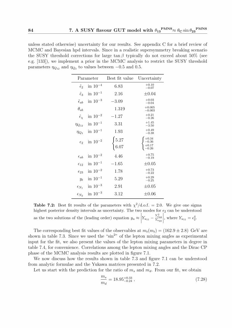
84 7. A SUSY flavour GUT model with θ13PMNS≈ θC sin θ23
PMNS
unless stated otherwise) uncertainty for our results. See appendix C for a brief review ofMCMC and Bayesian hpd intervals. Since in a realistic supersymmetry breaking scenariothe SUSY threshold corrections for large tan β typically do not exceed about 50% (seee.g. [133]), we implement a prior in the MCMC analysis to restrict the SUSY thresholdparameters ηQ12 and ηQ3 to values between −0.5 and 0.5.
Parameter Best fit value Uncertainty
ε2 in 10−4 6.83 +0.10−0.07
ε3 in 10−1 2.16 ±0.04
εab in 10−3 −3.09 +0.03−0.04
θab 1.319 +0.005−0.003
εχ in 10−2 −1.27 +0.21−0.26
ηQ12 in 10−1 3.31 +1.45−3.50
ηQ3 in 10−1 1.93 +0.49−0.38
ε2 in 10−2
5.27
6.07
+0.34−0.36+0.17−0.26
εab in 10−2 4.46 +0.75−0.19
ε12 in 10−1 −1.65 ±0.05
ε23 in 10−2 1.78 +0.73−0.22
yt in 10−1 5.29 +0.29−0.25
εN1 in 10−3 2.91 ±0.05
εN2 in 10−3 3.12 ±0.06
Table 7.2: Best fit results of the parameters with χ2/d.o.f. = 2.0. We give one sigmahighest posterior density intervals as uncertainty. The two modes for ε2 can be understood
as the two solutions of the (leading order) equation yu ≈∣∣∣∣Yu11 −
Y 2u12Yu22
∣∣∣∣, where Yu11 = ε42.
The corresponding best fit values of the observables at mt(mt) = (162.9± 2.8) GeV areshown in table 7.3. Since we used the “sin2” of the lepton mixing angles as experimentalinput for the fit, we also present the values of the lepton mixing parameters in degree intable 7.4, for convenience. Correlations among the lepton mixing angles and the Dirac CPphase of the MCMC analysis results are plotted in figure 7.1.
We now discuss how the results shown in table 7.3 and figure 7.1 can be understoodfrom analytic formulae and the Yukawa matrices presented in 7.2.
Let us start with the prediction for the ratio of ms and md. From our fit, we obtain
ms
md
= 18.95+0.33−0.24 , (7.28)

7.4 Phenomenology 85
øø
34é
36é
38é
40é
42é
44é
46é
8.5é
9.0é
9.5é
10.0é
10.5é
Θ23PMNS
Θ13PMNS
(a)
øø
32.5é33.0
é33.5
é34.0
é34.5
é35.0
é35.5
é36.0
é
8.5é
9.0é
9.5é
10.0é
10.5é
Θ12PMNS
Θ13PMNS
(b)
øø
34é
36é
38é
40é
42é
44é
46é
32.5é
33.0é
33.5é
34.0é
34.5é
35.0é
35.5é
36.0é
Θ23PMNS
Θ12PMNS
(c)
øø
260é262
é264
é266
é268
é270
é272
é274
é
32.5é
33.0é
33.5é
34.0é
34.5é
35.0é
35.5é
36.0é
∆PMNS
Θ12PMNS
(d)
øø
260é262
é264
é266
é268
é270
é272
é274
é
8.5é
9.0é
9.5é
10.0é
10.5é
∆PMNS
Θ13PMNS
(e)
øø
260é262
é264
é266
é268
é270
é272
é274
é
34é
36é
38é
40é
42é
44é
46é
∆PMNS
Θ23
PMNS
(f)
Figure 7.1: Correlations among the lepton mixing angles and the Dirac CP phase. Theblack star marks the best fit value, the yellow and grey regions give the one and threesigma hpd regions obtained from the MCMC analysis, respectively. The dashed grey linesindicate the one sigma intervals for the measured observables.

86 7. A SUSY flavour GUT model with θ13PMNS≈ θC sin θ23
PMNS
Observable Value at mt(mt) Best fit result Uncertainty
mu in MeV 1.22 +0.48−0.40 1.22 +0.49
−0.40
mc in GeV 0.59 ±0.08 0.59 ±0.08
mt in GeV 162.9 ±2.8 162.89 +2.62−2.36
md in MeV 2.76 +1.19−1.14 2.73 +0.30
−0.70
ms in MeV 52 ±15 51.66 +5.60−13.68
mb in GeV 2.75 ±0.09 2.75 ±0.09
me in MeV 0.485 ±1% 0.483 ±0.005
mµ in MeV 102.46 ±1% 102.83 +1.01−0.98
mτ in MeV 1742 ±1% 1741.75 +17.38−17.10
sin θC 0.2254 ±0.0007 0.2255 ±0.0007
sin θCKM23 0.0421 ±0.0006 0.0422 ±0.0006
sin θCKM13 0.0036 ±0.0001 0.0036 ±0.0001
δCKM in 69.2 ±3.1 65.65 +1.78−0.53
sin2 θPMNS12 0.306 ±0.012 0.317 ±0.006
sin2 θPMNS23 0.437 +0.061
−0.031 0.387 +0.017−0.023
sin2 θPMNS13 0.0231 +0.0023
−0.0022 0.0269 +0.0011−0.0015
δPMNS in - 268.79 +1.32−1.72
ϕPMNS2 in - 297.34 +8.66
−10.01
∆m212 in 10−5 eV2 7.45 +0.19
−0.16 7.45 +0.18−0.17
∆m231 in 10−3 eV2 2.421 +0.022
−0.023 2.421 +0.022−0.023
Table 7.3: Experimental values, best fit results, and uncertainties of the observables atmt(mt). We give one sigma highest posterior density intervals as uncertainty. Note thatalthough the masses of the charged leptons are known far more precise than listed here, weset an 1% uncertainty for the experimental values, which is roughly the accuracy of the oneloop calculation used here.
which is in excellent agreement with (2.38)
ms
md
= 18.9± 0.8 , (7.29)
obtained from experiments [22]. This can be understood from our choice of CG factors,
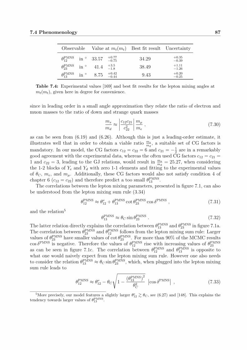
7.4 Phenomenology 87
Observable Value at mt(mt) Best fit result Uncertainty
θPMNS12 in 33.57 +0.77
−0.75 34.29 +0.35−0.39
θPMNS23 in 41.4 +3.5
−1.8 38.49 +1.11−1.26
θPMNS13 in 8.75 +0.42
−0.44 9.43 +0.20−0.25
Table 7.4: Experimental values [169] and best fit results for the lepton mixing angles atmt(mt), given here in degree for convenience.
since in leading order in a small angle approximation they relate the ratio of electron andmuon masses to the ratio of down and strange quark masses
ms
md
≈∣∣∣∣c12c21
c222
∣∣∣∣ mµ
me
, (7.30)
as can be seen from (6.19) and (6.26). Although this is just a leading-order estimate, itillustrates well that in order to obtain a viable ratio ms
md, a suitable set of CG factors is
mandatory. In our model, the CG factors c12 = c22 = 6 and c21 = −12
are in a remarkablygood agreement with the experimental data, whereas the often used CG factors c12 = c21 =1 and c22 = 3, leading to the GJ relations, would result in ms
md= 25.27, when considering
the 1-2 blocks of Ye and Yd with zero 1-1 elements and fitting to the experimental valuesof θC , me, and mµ. Additionally, these CG factors would also not satisfy condition 4 ofchapter 6 (c12 = c22) and therefore predict a too small θPMNS
13 .The correlations between the lepton mixing parameters, presented in figure 7.1, can also
be understood from the lepton mixing sum rule (3.34)
θPMNS12 ≈ θν12 + θPMNS
13 cot θPMNS23 cos δPMNS , (7.31)
and the relation5
θPMNS13 ≈ θC sin θPMNS
23 . (7.32)
The latter relation directly explains the correlation between θPMNS13 and θPMNS
23 in figure 7.1a.The correlation between θPMNS
23 and θPMNS12 follows from the lepton mixing sum rule: Larger
values of θPMNS23 have smaller values of cot θPMNS
23 . For more than 90% of the MCMC resultscos δPMNS is negative. Therefore the values of θPMNS
12 rise with increasing values of θPMNS23
as can be seen in figure 7.1c. The correlation between θPMNS12 and θPMNS
13 is opposite towhat one would naively expect from the lepton mixing sum rule. However one also needsto consider the relation θPMNS
13 ≈ θC sin θPMNS23 , which, when plugged into the lepton mixing
sum rule leads to
θPMNS12 ≈ θν12 − θC
√1− (θPMNS
13 )2
θ2C
∣∣cos δPMNS∣∣ , (7.33)
5More precisely, our model features a slightly larger θe12 & θC , see (6.27) and [148]. This explains thetendency towards larger values of θPMNS
13 .

88 7. A SUSY flavour GUT model with θ13PMNS≈ θC sin θ23
PMNS
where the negative sign of cos δPMNS is written explicitly. This explains the rising of θPMNS12
with increasing θPMNS13 seen in figure 7.1b. The correlation in figure 7.1d is again obvious
from the lepton mixing sum rule. Naively one would not expect correlations betweenδPMNS and the lepton mixing angles θPMNS
13 and θPMNS23 , respectively. The correlations seen
in figures 7.1e and 7.1f however follow indirectly from the other correlations discussedabove.
7.4.3 Discussion of the results
We close this chapter with a discussion of the various predictions of our model and howthe model potentially can be falsified with future experiments.
• Our best fit values θPMNS13 = 9.44+0.20
−0.25 and θPMNS23 = 38.49+1.11
−1.26 lie within their re-spective 2σ intervals reported in [169]. The correlation between θPMNS
13 and θPMNS23 in
figure 7.1a shows that our model favours slightly smaller values of θPMNS23 and slightly
larger values of θPMNS13 than in [169], whereas the most recent global fit results [62],
given in (6.2), have a tendency in the opposite direction. Note however, that the uncer-tainty of the individual measurements is still comparatively large, such as for instanceθPMNS
13 = 8.29+0.85
−0.72 reported by the RENO collaboration [170] and the one sigma in-terval of [38.6, 53.7] reported by the NOνA collaboration for θPMNS
23 [151]. The latestresult from DayaBay on the other hand is θPMNS
13 = 8.42+0.26
−0.25 [171]. Therefore, a moreprecise determination of θPMNS
13 and θPMNS23 is needed to test our model in the future.
• For the yet unmeasured Dirac CP phase of the PMNS matrix we predict
δPMNS = 268.79+1.32
−1.72 , (7.34)
which is in agreement with the results from recent global fits (3.37) δPMNS = 306+39
−70 .
• From the prediction of δPMNS follows that the cos δPMNS term in the lepton mixing sumrule leads to a negative correction to the TBM prediction of 35.3 for the solar mixingangle. We find θPMNS
12 = 34.29+0.35
−0.40 , which is within the one sigma interval of [169] andjust 0.03 outside of the one sigma interval reported in the recent global fit [62]. Likefor θPMNS
13 , figure 7.1c suggests slightly smaller values for θPMNS23 than currently reported.
• In the quark sector, our model predicts a CKM phase of δCKM = 65.65+1.78
−0.53 , whichis a slight discrepancy to the experimental value of 69.2 ± 3.1. With future, moreprecise measurements of δCKM our model thus could be falsified. As already discussedin (7.28), the model predicts ms
md= 18.95+0.33
−0.24, which is currently in excellent agreementwith experiments, but will be tested further in the future.
• Finally, we discuss our prediction for the Majorana phase
ϕPMNS2 = 297.34+8.66
−10.01 , (7.35)

7.4 Phenomenology 89
which is extremely difficult to be tested, due to the normal ordering of neutrino masses.The effective Majorana mass parameter (3.38), which is determined in neutrino-lessdouble beta decay experiments, is given by
〈mββ〉 =
∣∣∣∣(V PMNSe2
)2√
∆m221 +
(V PMNSe3
)2√
∆m231
∣∣∣∣ =(2.31+0.12
−0.09
)· 10−3 eV , (7.36)
which is far below the sensitivity of current experiments. Of course, a discovery ofneutrino-less double beta decay or of an inverse neutrino mass ordering would falsify ourmodel. Note however, that if a non-vanishing mass for the lightest neutrino ν1 wouldbe discovered, our model could simply be rearranged – with an appropriate adjustmentof shaping symmetries and messenger sector – by adding a third heavy right-handedneutrino and corresponding flavon field.
To conclude this chapter, we have successfully constructed a first SUSY flavour GUTmodel featuring θPMNS
13 ≈ θC sin θPMNS23 . Let us remark at this point, we do not consider our
model as the final model, rather it should be viewed as class of models, yielding realisticquark-lepton mass ratios and mixing angles relations. For example, the set of shapingsymmetries and messenger fields can be understood as proof of principle, instead of beingan one-of-a-kind realisation of our model’s features.
A complete SUSY flavour GUT model will have to include a successful SUSY breakingmechanism, a viable GUT Higgs sector, and a discussion on proton decay, among others.Some of this questions will be approached in chapters 9 and 10, where we discuss a so-lution to the doublet-triplet splitting problem in the context of flavour GUT models andpresent detailed calculations of the SUSY threshold corrections, which have been simplyapproximated as model parameters in this chapter.

CHAPTER 8
A SUSY flavour GUT model with inverseneutrino mass ordering
It is interesting to note that the vast majority of SUSY GUT models in the literature (seee.g. [172]) feature a normal neutrino mass ordering, whereas only few such models predictan inverted neutrino mass ordering. In this chapter we present our work [3] and constructa predictive and relatively simple SUSY SU(5) × A4 flavour GUT model, in which aninverse neutrino mass hierarchy is realised without fine-tuning of parameters. We followthe general procedure outlined in chapter 7 and both models share some of their properties,in particular the relation
θPMNS13 ≈ θC sin θPMNS
23 , (8.1)
by following the conditions of chapter 6. Other shared features are the novel CG factors−1
2, 6, and −3
2to obtain viable quark-lepton mass ratios, and spontaneous CP-symmetry
breaking by CP-violating vevs of flavon fields leading to α ≈ 90 in the quark unitaritytriangle.
Besides these shared features, there are also important differences, mainly due to thedifferent neutrino sector. These differences not only change the predictions in the leptonsector, but also in the quark sector, and will allow to discriminate between the two modelsusing the results of present and future experiments.
8.1 Constructing an inverted neutrino hierarchy
If the neutrino mass ordering would be measured to be inverse, it would imply that atleast two of the neutrino masses, namely m1 and m2, are almost degenerate, i.e. with masssplittings much smaller than the mass eigenvalues. Often, in order to realise such a smallneutrino mass splitting, an effective “special” lepton number symmetry like Le − Lµ − Lτ[173] or more generally some U(1) flavour symmetry is appealed to, yielding a mass matrix

8.1 Constructing an inverted neutrino hierarchy 91
for the light neutrinos of the form
mν ∼
0 ? ?? 0 0? 0 0
. (8.2)
Such symmetries have been used to construct GUT models (e.g. [174, 175]), but realisingan inverse mass ordering often turns out to be more involved than realising a normal one.
As discussed in 3.3, a promising approach for explaining an inverse mass ordering is toconsider a (mostly) off-diagonal mass matrix MR for two of the right-handed neutrinos,e.g.
MR = MR
(ε 11 0
), (8.3)
so that the two right-handed neutrinos form a (quasi-)Dirac pair with (almost) degenerateMajorana masses. The small entry ε in the 1-1 position of MR lifts the degeneracy of theright-handed neutrino masses and is in turn also responsible for the small mass splittingbetween the light neutrino masses m1 and m2, as seen below. With a neutrino Yukawacoupling matrix given by (3.44)
Yν =
a 00 b0 c
, (8.4)
the seesaw formula (3.7) yields the light neutrino mass matrix
mν =
0 B CB 0 0C 0 0
+ α
0 0 00 B C0 C C2/B
, (8.5)
with
B ≡ −b a v2u
2MR
, C ≡ −c a v2u
2MR
, and α ≡ −ε ba. (8.6)
The first part leads to two light neutrinos ν1, ν2 with exactly degenerate masses [173], whilethe second part can be considered as a small perturbation which induces the solar masssplitting ∆m2
12. Here we consider only two right-handed neutrinos, thus the mass of thelightest neutrino is zero, m3 = 0, and our model features a strong inverse neutrino masshierarchy, although strictly speaking the hierarchy is only between m3 and m1 ≈ m2.
Implementation in flavour models: In order to construct a flavour model which re-alises an inverse neutrino mass hierarchy, we thus need to have the columns of the neutrinoYukawa matrix (8.4) be generated by vevs of flavon fields, which are triplets under a non-Abelian discrete flavour symmetry group like A4. Additionally, the right-handed neutrinosneed to be charged under the model’s shaping symmetry such that the desired mass matrix

92 8. A SUSY flavour GUT model with inverse neutrino mass ordering
(8.5) is obtained. In 8.3 we present an alignment superpotential which enforces flavon fieldsto obtain vevs pointing in the specific directionsa0
0
and
0bc
(8.7)
in flavour space.
Mixing angles and the Dirac CP phase: One can calculate the non-vanishing neu-trino masses mi and the mixing angles θνij in leading order in α
−∆m232 = m2
2 ≈ B2 + C2 , (8.8a)
∆m221 = m2
2 −m21 ≈ 2α
(B2 + C2)3/2
|B| , (8.8b)
tan θν12 ≈∣∣∣∣∣1− α
2
√B2 + C2
|B|
∣∣∣∣∣ ≈∣∣∣∣1 +
1
4
∆m2sol
∆m2atm
∣∣∣∣ , (8.8c)
tan θν23 =
∣∣∣∣CB∣∣∣∣ , (8.8d)
θν13 = 0 , (8.8e)
where all parameters were assumed to be real. The small mass splitting between ν1 andν2 thus directly results from the correction α, whose smallness can be naturally explainedas being due to a higher-dimensional operator, such that no unnatural cancellation of apriori unrelated parameters is necessary.
Looking at the neutrino mixing angles, we find that θν23 is a free parameter. On the otherhand, the deviation from tan θν12 = 1 is smaller than 10−2, which amounts to a negligiblysmall deviation from maximal θν12 = 45, and the 1-3 mixing in the neutrino sector isfixed to zero. Thus, it is in accordance with condition 1 of chapter 6 and it opens upthe possibility to explain θPMNS
13 ≈ θC sin θPMNS23 via charged lepton corrections and suitable
CG factors in GUTs. As discussed in 6.5, via the lepton mixing sum rule (6.47) maximalθν12 and the observed value of θPMNS
12 require a Dirac CP phase of δPMNS = 180. Notethat all necessary assumptions of chapter 6 like θe13 ≈ θe23 ≈ 0, and a Dirac CP phase ofδPMNS = 180 will be built-in features of our model, as we discuss in the following section.
8.2 The model
As in the previous chapter, we embed the three families of the MSSM matter superfieldsDci and Li into one A4 triplet F , transforming as 5 of SU(5), and the remaining matter
superfields into three A4-invariant singlets Ti, one for each family, which transform as 10under SU(5). We introduce two right-handed neutrinos N c
1 and N c2 as singlets under SU(5)
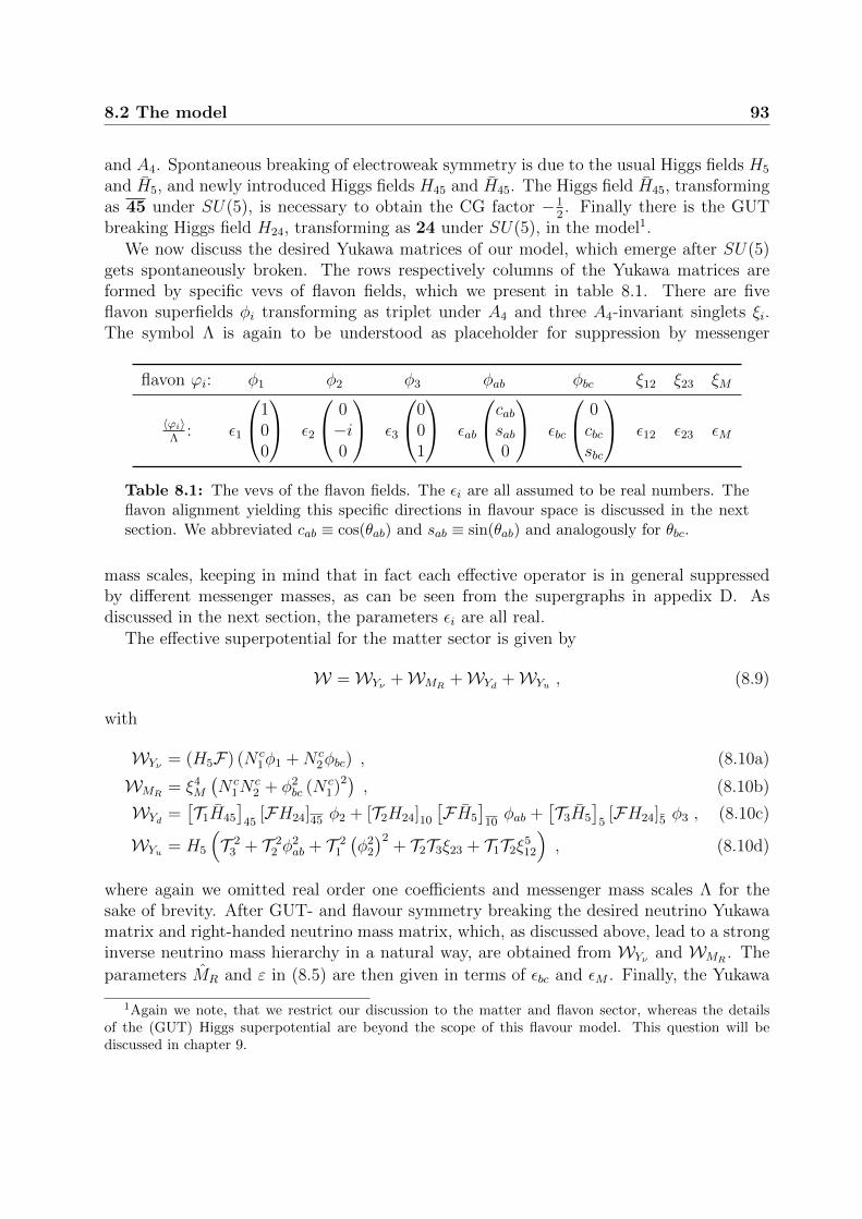
8.2 The model 93
and A4. Spontaneous breaking of electroweak symmetry is due to the usual Higgs fields H5
and H5, and newly introduced Higgs fields H45 and H45. The Higgs field H45, transformingas 45 under SU(5), is necessary to obtain the CG factor −1
2. Finally there is the GUT
breaking Higgs field H24, transforming as 24 under SU(5), in the model1.We now discuss the desired Yukawa matrices of our model, which emerge after SU(5)
gets spontaneously broken. The rows respectively columns of the Yukawa matrices areformed by specific vevs of flavon fields, which we present in table 8.1. There are fiveflavon superfields φi transforming as triplet under A4 and three A4-invariant singlets ξi.The symbol Λ is again to be understood as placeholder for suppression by messenger
flavon ϕi: φ1 φ2 φ3 φab φbc ξ12 ξ23 ξM
〈ϕi〉Λ
: ε1
100
ε2
0−i0
ε3
001
εab
cabsab0
εbc
0cbcsbc
ε12 ε23 εM
Table 8.1: The vevs of the flavon fields. The εi are all assumed to be real numbers. Theflavon alignment yielding this specific directions in flavour space is discussed in the nextsection. We abbreviated cab ≡ cos(θab) and sab ≡ sin(θab) and analogously for θbc.
mass scales, keeping in mind that in fact each effective operator is in general suppressedby different messenger masses, as can be seen from the supergraphs in appedix D. Asdiscussed in the next section, the parameters εi are all real.
The effective superpotential for the matter sector is given by
W =WYν +WMR+WYd +WYu , (8.9)
with
WYν = (H5F) (N c1φ1 +N c
2φbc) , (8.10a)
WMR= ξ4
M
(N c
1Nc2 + φ2
bc (N c1)2) , (8.10b)
WYd =[T1H45
]45
[FH24]45 φ2 + [T2H24]10
[FH5
]10φab +
[T3H5
]5
[FH24]5 φ3 , (8.10c)
WYu = H5
(T 2
3 + T 22 φ
2ab + T 2
1
(φ2
2
)2+ T2T3ξ23 + T1T2ξ
512
), (8.10d)
where again we omitted real order one coefficients and messenger mass scales Λ for thesake of brevity. After GUT- and flavour symmetry breaking the desired neutrino Yukawamatrix and right-handed neutrino mass matrix, which, as discussed above, lead to a stronginverse neutrino mass hierarchy in a natural way, are obtained from WYν and WMR
. The
parameters MR and ε in (8.5) are then given in terms of εbc and εM . Finally, the Yukawa
1Again we note, that we restrict our discussion to the matter and flavon sector, whereas the detailsof the (GUT) Higgs superpotential are beyond the scope of this flavour model. This question will bediscussed in chapter 9.

94 8. A SUSY flavour GUT model with inverse neutrino mass ordering
matrices of the quarks and charged leptons are given by
Yd =
0 −iε2 0εabcab εabsab 0
0 0 ε3
, Ye =
0 6εabcab 0i1
2ε2 6εabsab 0
0 0 −32ε3
, Yu =
ε42 ε512 0ε512 ε2ab ε23
0 ε23 yt
,
(8.11)where we defined
εi ≡〈H24〉
Λεi (8.12)
for convenience. Note that Yd and Yu fulfil the necessary conditions θu13, θd13 ≈ 0 for the
quark mixing and phase sum rule, respectively, such that θd12 ≈ θC and a right-angled quarkunitarity triangle is obtained.
As discussed in 7.1, in order to construct a viable and predictive flavour GUT model,it is necessary to identify a shaping symmetry and a set of messenger fields, that, whenintegrated out, gives rise to the effective superpotential (8.10). Specifically, no effectiveoperators must exist which spoil the features of our Yukawa matrices, e.g. by generatingunwanted CG factors or relevant corrections to the desired structure of the Yukawa ma-trices (8.4), (8.11), and of the right-handed neutrino mass matrix (8.5). In appendix Dwe therefore present the model’s shaping symmetry and messenger fields, and explicitlyconstruct the renormalisable superpotential which yields (8.10) after the messenger fieldsare integrated out. With this messenger sector at hand, sub-leading corrections from e.g.higher-dimensional operators or from canonical normalisation can be neglected.
8.3 Flavon alignment
In this section we present the flavon alignment superpotential, which enforces the flavonvevs into the specific directions in flavour space shown in table 8.1. We introduce thedriving fields Si, Di, Oi, and O′i, which are all singlets under SU(5) and – with the exceptionof O′i, which transform as 1′ under A4 – invariant singlets 1 under A4. In appendix D, allflavon and driving superfields are listed in the lower part of table D.3, together with theircharges under the imposed symmetries. The effective flavon alignment superpotential isgiven by
Wflavon =Wφi +Wab +Wbc +WM +W12 , (8.13)
where
Wφi = S2
((φ2
2
)3+M2
2
)+∑i∈1,3
Si(φ2i −M2
i
)+
3∑i,j=1j>i
(O′i;j(φiφj)1′′ +Oi;j(φiφj)
),
(8.14a)
Wab = Sab((φab ? φab)
2 ξ223 −M2
ab
)+Dα
ab
(φ2ab + λabξ
223
)+Dβ
ab (φab ? φab)φab +Dγab
((φ2ab
)1′
(φ2ab
)1′′
+ kab (φab ? φab)2) , (8.14b)

8.3 Flavon alignment 95
Wbc = Sbc((φbc ? φbc)
2 φ2bc −M2
bc
)+Dβ
bc (φbc ? φbc)φbc
+Dγbc
((φ2bc
)1′
(φ2bc
)1′′
+ kbc (φbc ? φbc)2) , (8.14c)
WM = SM(ξ6M −M2
M
), (8.14d)
W12 = S12
(ξ6
12 −M212
). (8.14e)
Since CP symmetry is assumed to be broken only spontaneously, the constants ki and Mi
are real. In addition we assume M2i > 0 everywhere. The terms W12 and WM lead to vevs
with discrete phases as discussed in 7.3, of which we select the real phases. The alignmentsuperpotentialWab is the same as in chapter 7, i.e. the term containing Sab determines themagnitude and a discrete global phase of the product of φab and ξ23, whereas the individualmagnitudes are fixed by the F -term of Dα
ab. The term with the driving superfield Dβab sets
one of the components of 〈φab〉 to zero and the relative magnitude or the relative phaseis finally enforced as in (7.25) by the value of kab. Similarly, replacing a, b → b, c andkab → kbc, respectively, the vev of the flavon superfield φbc, which appears in the neutrinoYukawa matrix (8.4), is obtained. Let us now discuss the remaining flavon vevs in detail.
Wφi: Let us denote the components of φi with x1, x2, and x3, and the components of φjwith y1, y2, and y3. The F -term equations corresponding to Oi;j and O′i;j then take theform
x1y1 + x2y2 + x3y3 = 0 , (8.15a)
and
x1y1 + ωx2y2 + ω2x3y3 = 0 , (8.15b)
respectively, where for each pair Oi;j and O′i;j there is one such system of equations. Thereare two classes of solutions to the system (8.15), namely
x1y1 = x2y2 = x3y3 = 0 , (8.16a)
and
x1y1 = γ , x2y2 = ω γ , x3y3 = ω2 γ , (8.16b)
where γ is a complex constant γ 6= 0. There is no consistent solution for φ1, φ2, and φ3 thatsatisfies (8.16a) for one pair Oi;j and O′i;j and (8.16b) for another pair. The only solutionsto all three equation pairs are thus either all of type (8.16a) or all of type (8.16b). Theyare given by
φ1 ∝
100
, φ2 ∝
010
, φ3 ∝
001
, (8.17a)
96 8. A SUSY flavour GUT model with inverse neutrino mass ordering
or permutations thereof, and
φi ∝
1√ωω
, for i = 1, 2, 3 . (8.17b)
Which solution is realised depends on the terms containing the driving superfields Si. Sincefor solution (8.17b) the invariant φ2
i vanishes for all φi, in our superpotential (8.14a) onlysolution (8.17a) is generated. Again, their phases take on discrete values and we select animaginary vev for φ2 and real vevs for φ1 and φ3, as shown in table 8.1.
8.4 Phenomenology
We now turn to a discussion of the model’s phenomenology. There are 14 free parameters:ε2, ε3, εab, θab, ηQ12 , and ηQ3 parametrise the Yukawa matrices Yd and Ye. The parametersyt, εab, ε2, ε12, and ε23 enter Yu, where, since εab and ε2 do only appear at quadratic andquartic order, respectively, we restrict them to positive values. As shown in (8.5), theeffective mass matrix of the light neutrinos depends only on three parameters after theheavy right-handed neutrinos are integrated out. It is thus possible to fix two out of thefive parameters in the neutrino sector: While we use ε1, εbc, and θbc to fit the GUT scaleYukawa neutrino matrix Yν , we set the parameters of MR to MR = 2 · 1010 GeV andε = 10−2. Again, for neutrino Yukawa couplings much smaller than one, which impliesthat Yν is irrelevant in the RGEs, our choice of MR does not affect the fit. The neutrinosector is therefore given by
Yν =
ε1 00 εbc cos θbc0 εbc sin θbc
, MR = 2 · 1010 GeV ·(
10−2 11 0
). (8.18)
We follow the same numerical procedure as described in 7.4.1 and again set tan β = 40due to the need of tan β-enhanced SUSY threshold corrections in order for the models’sCG factors to be viable. Once again the SUSY threshold corrections at MSUSY = 1 TeVare included by the approximate matching relations (7.26) as model parameters assumingdegenerate first and second family sfermion masses.
Analogous to our model in chapter 7, we here report our results from [3], where we used2013 data [167–169] for the experimental values at the low energy scale mt(mt). We willdiscuss our results in the light of newly available data at the end of the chapter.
Note that with a strong inverse neutrino mass hierarchy and massless ν3, the singlephysical Majorana phase predicted by our model is given by
φPMNS = φPMNS2 − φPMNS
1 . (8.19)
With the prediction of the Dirac CP phase δPMNS and from fitting 14 parameters to 18measured observables, it follows that our model makes six predictions.

8.4 Phenomenology 97
8.4.1 Results
We find a best fit point with a total χ2 = 4.6. The reduced χ2 is thus χ2/d.o.f. = 1.1.Compared to χ2/d.o.f. = 2.0 in the fit of the normal hierarchy model of chapter 7, wethus obtain an even better agreement with the measured observables. In table 8.2 wepresent the best fit values of our parameters, together with uncertainties obtained as onesigma hpd intervals from a MCMC analysis using a Metropolis algorithm. Note that againwe enforce a prior on the SUSY threshold correction parameters to restrict their absolutevalues |ηi| < 0.5, justified by the typical size of SUSY threshold corrections in commonSUSY breaking scenarios.
Parameter Best fit value Uncertainty
ε2 in 10−4 6.71 +0.08−0.07
ε3 in 10−1 2.23 ±0.03
εab in 10−3 3.03 ±0.03
θab 1.314 +0.004−0.003
ηQ12 in 10−1 3.36 +1.35−2.50
ηQ3 in 10−1 1.64 +0.44−0.37
ε2 in 10−2
5.22
6.04
+0.34−0.37+0.18−0.23
εab in 10−2 4.45 +0.53−0.18
ε12 in 10−1 −1.64 +0.05−0.04
ε23 in 10−2 1.76 +0.49−0.16
yt in 10−1 5.30 +0.35−0.27
ε1 in 10−3 3.21 +0.11−0.09
εbc in 10−3 −5.12 +0.11−0.15
θbc 0.71 ±0.02
Table 8.2: Best fit results of the model’s parameters with χ2/d.o.f. = 1.1. The uncertain-ties are given as one sigma hpd intervals. Again, the two modes for ε2 can be understood
as the two solutions of the (leading order) equation yu ≈∣∣∣∣Yu11 −
Y 2u12Yu22
∣∣∣∣, where Yu11 = ε42.
In tables 8.3 and 8.4 the best fit values of the observables at mt(mt) are shown.Correlations among the lepton mixing angles in the MCMC analysis are shown in fig-ure 8.1. Like in 7.4.2, they can be understood in terms of the lepton mixing sum ruleθPMNS
12 ≈ θν12 + θPMNS13 cot θPMNS
23 cos δPMNS and θPMNS13 ≈ θC sin θPMNS
23 . The noticeable differ-ence in the shape of figures 7.1c and 8.1c is due to the different values of δPMNS. Whereas

98 8. A SUSY flavour GUT model with inverse neutrino mass ordering
cos δPMNS almost vanishes in 7.4.2, leading to θPMNS12 given almost exclusively in terms of
θν12, the value of δPMNS = 180 in the inverse hierarchy model maximises the contributionof θPMNS
23 to θPMNS12 , leading to a large deviation of θPMNS
12 from θν23 = 45 and explaining thelarger hpd regions in figure 8.1c.
øø
34é
36é
38é
40é
42é
44é
46é
8.5é
9.0é
9.5é
10.0é
10.5é
Θ23PMNS
Θ13
PMNS
(a)
øø
32.0é32.5
é33.0
é33.5
é34.0
é34.5
é35.0
é
8.5é
9.0é
9.5é
10.0é
10.5é
Θ12PMNS
Θ13
PMNS
(b)
øø
34é
36é
38é
40é
42é
44é
46é
32.0é
32.5é
33.0é
33.5é
34.0é
34.5é
35.0é
Θ23PMNS
Θ12
PMNS
(c)
Figure 8.1: Correlations among the lepton mixing angles. The black star marks the bestfit value. The blue and golden regions give the one sigma and three sigma hpd regionsobtained from the MCMC analysis, respectively. The dashed grey lines indicate the onesigma intervals for the measured observables.
As for the normal hierarchy model in chapter 7, we obtain an excellent prediction for
ms
md
= 18.55+0.26−0.24 , (8.20)
due to the specific CG factors in our model.

8.4 Phenomenology 99
Observable Value at mt(mt) Best fit result Uncertainty
mu in MeV 1.22 +0.48−0.40 1.22 +0.50
−0.39
mc in GeV 0.59 ±0.08 0.59 +0.07−0.09
mt in GeV 162.9 ±2.8 162.91 +3.35−2.44
md in MeV 2.76 +1.19−1.14 2.73 +0.25
−0.54
ms in MeV 52 ±15 50.70 +4.86−9.72
mb in GeV 2.75 ±0.09 2.75 ±0.09
me in MeV 0.485 ±1% 0.483 ±0.005
mµ in MeV 102.46 ±1% 102.87 +1.04−0.91
mτ in MeV 1742 ±1% 1741.99 +16.84−17.70
sin θC 0.2254 ±0.0007 0.2255 ±0.0007
sin θCKM23 0.0421 ±0.0006 0.0421 ±0.0006
sin θCKM13 0.0036 ±0.0001 0.0036 ±0.0001
δCKM in 69.2 ±3.1 69.27 +0.91−0.69
sin2 θPMNS12 0.306 ±0.012 0.303 ±0.005
sin2 θPMNS23 0.437 +0.061
−0.031 0.397 +0.023−0.022
sin2 θPMNS13 0.0231 +0.0023
−0.0022 0.0267 +0.0016−0.0015
δPMNS in - 180 -
ϕPMNS in - 180 -
∆m212 in 10−5 eV2 7.45 +0.19
−0.16 7.45 +0.18−0.17
∆m232 in 10−3 eV2 −2.410 +0.062
−0.063 −2.410 +0.062−0.064
Table 8.3: Experimental values, best fit results, and uncertainties of the observables atmt(mt). We give one sigma highest posterior density intervals as uncertainty. δPMNS andϕPMNS are exactly 180, since Yν is real and the phase of Ye21 can be absorbed by the right-handed electron field. Note that although the masses of the charged leptons are known farmore precise than listed here, we set an 1% uncertainty for the experimental values, whichis roughly the accuracy of the one loop calculation used here.
The sign of the larger neutrino mass splitting ∆m23i will be in the focus of the next
round of neutrino oscillation experiments and will allow to distinguish between inverse andnormal neutrino mass ordering. Furthermore, neutrino-less double beta decay experiments

100 8. A SUSY flavour GUT model with inverse neutrino mass ordering
Observable Value at mt(mt) Best fit result Uncertainty
θPMNS12 in 33.57 +0.77
−0.75 33.38 +0.30−0.28
θPMNS23 in 41.4 +3.5
−1.8 39.06 +1.33−1.32
θPMNS13 in 8.75 +0.42
−0.44 9.41 +0.28−0.27
Table 8.4: Experimental values [169] and best fit results for the lepton mixing angles atmt(mt), given here in degree for convenience.
will soon be able to test predictions from inverse neutrino mass ordering models. Ourmodel predicts an effective Majorana mass parameter (3.38) of
〈mββ〉 =
∣∣∣∣(V PMNSe1
)2√−∆m2
32 −∆m221 +
(V PMNSe2
)2√−∆m2
32
∣∣∣∣=(1.83+0.05
−0.06
)· 10−2 eV . (8.21)
This is in reach of future experiments, such as nEXO (see e.g. [176]) and AMoRE [177].
8.4.2 Discussion
In the following we turn to a detailed discussion of the fit results of our model, includingcomments regarding the more recent data for lepton mixing angles [62].
• Our model predicts the PMNS phases of
δPMNS = 180 and ϕPMNS = 180 . (8.22)
Since Yν is real and the phase of the 2-1 element of Ye can be absorbed by the right-handedelectron field Ec
1, the PMNS phases are fixed at the GUT scale and do not evolve underthe RGEs. Our model’s best fit value for the Dirac CP phases is marginally outside theone sigma interval of the recently reported hints towards δPMNS = 254 +63
−62 from globalfits assuming a inverse neutrino mass ordering (3.37). A future precise measurement ofδPMNS could decide whether our model agrees with the data or not.
• As for the normal hierarchy model in chapter 7, our inverse mass hierarchy model alsofeatures a best fit value θPMNS
13 = 9.41+0.28
−0.27 slightly larger than the reported experimentalvalue in [169], and a best fit value θPMNS
23 = 39.06+1.33
−1.32 slightly smaller than reportedin [169]. Both best fit points are within their respective two sigma intervals, however.
In the light of the recent global fit [62], the most drastic difference lies in the reportedvalue for θPMNS
23 , which, when an inverse neutrino mass ordering is assumed as prior,lies in the second octant θPMNS
23 = 49.5 +1.5
−2.2 , whereas the 2013 data [169] reporteda best fit point in the first octant for both, normal and inverse mass orderings. Iffuture measurements of θPMNS
23 would confirm a value larger than 45, it effectively would

8.4 Phenomenology 101
refute the relation θPMNS13 ≈ θC sin θPMNS
23 , especially since in the case of an inverse masshierarchy this relation is highly insensitive to corrections from RG running or canonicalnormalisation, as discussed in 6.4. Large corrections would be necessary however, tocure the bad contribution of sin θPMNS
23 > 1√2.
Let us remark at this point, that precise measurements of θPMNS23 are still work in progress,
e.g. by the NOνA collaboration, which reports an one sigma interval of [38.6, 53.7][151]. The subject whether θPMNS
23 lies in the first or second octant therefore remains animportant open question and in the future global fits might report θPMNS
23 < 45 again.
Future improvements on the determination of θPMNS23 and θPMNS
13 thus have the capabilityto falsify our model, or to strengthen the relation θPMNS
13 ≈ θC sin θPMNS23 with higher
precision.
• Finally, our model finds a best fit point θPMNS12 = 33.38+0.30
−0.28 , which lies within the onesigma range of the experimental values as reported in the 2013 [169] and 2015 data [62].
8.4.3 Phenomenological differences to the model of chapter 7
Let us close this chapter by discussing the differences between the SUSY flavour GUTmodels of [2] presented in chapter 7 and the model of [3] discussed in this chapter. Thereare five major differences between these models, summarised in table 8.5.
NH IH
∆m23i 2.421+0.022
−0.023 · 10−3 eV2 −2.410+0.062−0.064 · 10−3 eV2
〈mββ〉 2.31+0.12−0.09 · 10−3 eV 1.83+0.05
−0.06 · 10−2 eV
δPMNS 268.79+1.32
−1.72 180
θPMNS12 34.29+0.35
−0.39 33.38+0.30
−0.28
δCKM 65.65+1.78
−0.53 69.27+0.91
−0.69
Table 8.5: Major differences in the best fit results between the two SUSY flavour GUTmodels of [2] (NH) and [3] (IH).
The sign of the larger neutrino mass splitting ∆m232 (IH) respectively ∆m2
31 (NH) isthe defining characteristic of normal vs inverse hierarchy models. Its measurement is inthe focus of upcoming long baseline neutrino experiments, e.g. at DUNE [69]. Similarly,the different magnitudes of the effective Majorana mass 〈mββ〉 for neutrinoless double betadecay are a typical distinction between normal and inverse neutrino mass ordering.
The observed large value of θPMNS13 opens up the possibility of measuring the Dirac CP
phase δPMNS in long-baseline neutrino oscillation experiments. Therefore our two SUSYflavour GUT models models can also clearly be distinguished via their respective predic-tions of δPMNS, whose measurement is also a scientific goal of the DUNE experiment [69].
102 8. A SUSY flavour GUT model with inverse neutrino mass ordering
The lepton mixing angles in both models share the same characteristic correlations andthe differences between the best fit values turn out to be less than one degree. Since futuremore precise measurements of θPMNS
13 and θPMNS23 will support or disprove our models in
equal measure, they are not expected to distinguish our two models. A future 50 − 70km baseline reactor experiment though could measure θPMNS
12 with high precision [178],allowing to discriminate between the respective predictions of θPMNS
12 in the normal andinverse mass ordering models. Note however that the fit results for θPMNS
12 depend on theexperimental ranges for θPMNS
13 and θPMNS23 via the lepton mixing sum rule.
Finally let us note the remarkable fact that our models, although mainly distinct by theirneutrino sector, can furthermore be distinguished in the quark sector by their predictionsfor the CKM phase.

PART IV
Doublet-Triplet splitting in SUSYFlavour GUT models

CHAPTER 9
Towards predictive SUSY flavour SU(5)models with doublet-triplet splitting
Grand Unified Theories offer an attractive framework for flavour models, since they linkthe quark and lepton sectors of the MSSM. As discussed in chapters 4 and 5, they howeveralso feature potentially wrong predictions for proton decay. In the previous chapters wepresented two predictive SUSY flavour SU(5) GUT models, which successfully explainthe observed hierarchies of fermion masses and mixing angles. But in addition to correctpredictions for the flavour observables, a complete SUSY flavour GUT model also has toinclude a viable mechanism for GUT symmetry breaking, including sufficient suppressionof proton decay without unacceptably large fine-tuning.
In this chapter we present our results of [4] and introduce a novel version of the doublemissing partner mechanism (DMPM) solution to the doublet-triplet splitting problem,which can be combined with predictive models for the GUT scale quark-lepton Yukawacoupling ratios. Two explicit flavour models with different GUT scale predictions arepresented, including shaping symmetries and renormalisable messenger sectors.
9.1 The missing partner and double missing partner
mechanisms
Since we are considering SUSY SU(5) GUTs, the GUT scale of about 1016 GeV is largeenough to sufficiently suppress proton decay from dimension six GUT operators, as dis-cussed in 5.5. There we also discussed the doublet-triplet splitting problem arising fromrequiring sufficiently heavy Higgs colour triplets T (5) and T (5), which mediate dimensionfive proton decay, whereas the MSSM Higgs doublets have to remain light.
In SU(5) GUTs, one proposed solution to the DTS problem is the missing partnermechanism (MPM) [144] or its improved version, the double missing partner mechanism(DMPM) [179], which we will review briefly below.1 These solutions have been applied in
1In theories of extra dimensions, another solution exists, see e.g. [180].

9.1 The missing partner and double missing partner mechanisms 105
GUT models, but they either predict the unrealistic quark-lepton Yukawa relation Ye = Y Td
(e.g. [181]), the experimentally disfavoured combination of the Georgi-Jarlskog relations(4.28) (as e.g. in [182]), or they rely on linear combinations of GUT Yukawa operators(e.g. [183]), which again implies the loss of predictivity.
On the other hand, there exists a large number of GUT models which focus on theflavour sector, but do not include the (GUT) Higgs potential. It is therefore an interestingquestion to ask how the DTS problem can be resolved in predictive SUSY flavour GUTmodels, given the present rather precise experimental data on the fermion masses andmixing angles.
As successfully constructed in our two SUYS flavour GUT models of the previous chap-ters, we employ new Clebsch-Gordan factors emerging from higher-dimensional operatorscontaining a GUT breaking Higgs field in the adjoint representation, to arrive at experi-mentally favoured GUT scale Yukawa coupling ratios. In this chapter we present how thisapproach can be combined with a novel DMPM version for solving the DTS problem.
Let us now review the missing partner mechanisms. Note that throughout this section,for illustrative purposes, we consider that the bounds on proton decay rates require theeffective mass of the colour triplets (5.87) to be of at least Mdim=5
T ≈ 1017 GeV [82, 143],while the effective mass suppressing dimension six proton decay mediated by the colourtriplets (4.33) is required to be Mdim=6
T & 1012 GeV [82].
9.1.1 The missing partner mechanism
The basic idea of the MPM is the introduction of two new superfields Z50 and Z50 in 50and 50 representations of SU(5). The decomposition of 50 under the SM gauge group isgiven by
50 = (1,1)−2 + (3,1)− 13
+ (3,2)− 76
+ (6,1) 43
+ (6,3)− 13
+ (8,2) 12, (9.1)
which does not contain an SU(2)L doublet, but it includes an SU(3)C triplet. Thus, usingthe 50s as messenger fields to generate an effective mass term for H5 and H5 keeps theelectroweak doublets massless, while the colour triplets acquire masses of the order of theGUT scale.
Note that 50 is not in the SU(5) tensor product
24× 5 = 5 + 45 + 70 . (9.2)
Thus, instead of 24, the MPM contains a GUT breaking Higgs field H75 transforming as75 of SU(5) [184,185], since
75× 5 = 45 + 50 + 280 . (9.3)
The superpotential for the MPM is given by2
WMPM = H5H75Z50 + Z50H75H5 +M50Z50Z50 . (9.4)
2For readability we omit SU(5) indices and most order one coefficients in the superpotentials, exceptwhere they are relevant to the discussion.

106 9. Towards predictive SUSY flavour SU(5) models with DT splitting
Note that, because of75 ⊂ 24× 24 , (9.5)
H75 can be replaced by the effective combinationH2
24
Λin non-renormalisable theories, where
Λ denotes a general mass suppression [181], see also 9.2.2.With the triplet mass contribution from 〈H75〉 denoted by V , the mass matrices of the
Higgs fields H5, H5 and Z50, Z50 are given by
mD = 0 , mT =
(0 VV M50
), (9.6)
for the doublet and triplet components D and T of H5 and Z50, respectively. The dangerousterms for dimension five proton decay are obtained from the Yukawa couplings (5.83)
WYuk = TiFjH5 + TiTjH5 . (9.7)
To calculate the effective dimension five proton decay operators, all Higgs triplets fromall 5, 50, and their respective conjugate representations have to be integrated out, butonly the triplets in H5 and H5 couple to matter. We denote the triplet mass eigenvalueswith M1 and M2, and the corresponding mass eigenstates as T1 and T2, respectively. Thetriplets that couple to matter are given by the combinations
T (5) =∑i
U∗1iTi , T (5) =∑i
V1i¯Ti , (9.8)
where U and V are unitary matrices defined by mT = UmdiagT V †. Integrating out the
triplet mass eigenstates Ti leads to the effective dimension five operator for proton decay,which is proportional to the inverse of the effective triplet mass
(Mdim=5T )−1 ≡ U∗1i
(mdiagT
)−1
ijV1j = U∗1i
(mdiagT
)−1
ijV Tj1 = (m−1
T )11 . (9.9)
The Kahler potential for the MPM triplet superfields is given by
KT = T (5)T (5)∗ + T (5)T (5)∗ + T (50)T (50)∗ + T (50)T (50)∗ . (9.10)
When the heavy colour triplet mass eigenstates are also integrated out in KT , effectivedimension six Kahler operators emerge from inserting their equations of motion. Thenthe Lagrange density obtained from the D-term of the effective Kahler potential containsbaryon number violating four fermion operators, proportional to(
Mdim=6T
)−2 ≡ V1i
(mdiagT
)−1
ijU †jkUkm
(mdiagT
)−1
mlV †l1 =
(m−1T m†−1
T
)11
(9.11)
from T (r)T (r)∗ and to(Mdim=6
T
)−2 ≡(m†−1T m−1
T
)11
(9.12)

9.1 The missing partner and double missing partner mechanisms 107
from T (r)T (r)∗. With the mass matrix mT given in (9.6), the effective triplet mass is thus3
Mdim=5T =
(m−1T
)−1
11= − V 2
M50
, (9.13)
while the suppression of dimension six proton decay is given by(Mdim=6
T
)2=(Mdim=6
T
)2=(m−1T m†−1
T
)−1
11=
|V |4
|M50|2 + |V |2. (9.14)
Note that with a GUT scale value of V ≈ 1016 GeV and M50 below the Planck scale,the dimension six proton decay is suppressed sufficiently with values of Mdim=6
T between1013 and 1016 GeV.
The splitting between doublet and triplet masses is achieved since the doublets obtainno mass term. Using Mdim=5
T & 1017 GeV one obtains an upper bound for M50 . 1015 GeV.Having the large representations 50 and 50 enter the RGEs at such a low energy scale,however, leads to the breakdown of perturbativity just above the GUT scale. Thus, theMPM solves the DTS problem – but trades it for SU(5) becoming non-perturbative muchbelow the Planck scale Mpl.
9.1.2 The double missing partner mechanism
This trade-off can be avoided in the DMPM, where the number of Higgs fields in 5, 5,50, and 50 representations gets doubled [179]. The fields H5 and H5 couple to the matterfields Fi and Ti, whereas H ′5 and H ′5 do not. The superpotential for the DMPM is givenby
WDMPM = H5H75Z50 + Z50H75H′5 + H ′5H75Z
′50 + Z ′50H75H5
+M50Z50Z50 +M ′50Z
′50Z
′50 + µ′H ′5H
′5 . (9.15)
The mass matrices of the doublet and triplet components of the Higgs fields H5, H ′5, Z50,Z ′50 and their corresponding conjugated fields after H75 gets a vev V are given by
mD =
(0 00 µ′
), mT =
0 0 0 V0 µ′ V 0V 0 M50 00 V 0 M ′
50
. (9.16)
While the Higgs doublets coupling to matter remain massless, the second pair of Higgsdoublets contained in H ′5 and H ′5 has mass µ′. The improvement of the DMPM comparedto the MPM can be seen from the effective triplet mass
Mdim=5T =
(m−1T
)−1
11= − V 4
µ′M50M ′50
. (9.17)
3In the text when we quote numbers for Mdim=5T , Mdim=6
T , and Mdim=6T
we will always refer to theirabsolute values.

108 9. Towards predictive SUSY flavour SU(5) models with DT splitting
The same effective triplet mass of Mdim=5T ≈ 1017 GeV can now be obtained while keeping
high masses M50 ≈ M ′50 ≈ 1018 GeV, provided the heavier doublet pair has a (relatively)
small mass µ′ ≈ 1011 GeV. With the large representations of SU(5) having large masses,the perturbativity of the model can be preserved up to (almost) the Planck scale.
Dimension six proton decay is suppressed by
(Mdim=6
T
)2=(m−1T m†−1
T
)−1
11=
|V |8
|V |6 + |M50|2(|V |4 + |M ′
50µ′|2 + |V µ′|2
) ≈ (1014 GeV)2 ,
(9.18)(Mdim=6
T
)2=(m†−1T m−1
T
)−1
11=
|V |8
|V |6 + |M ′50|2
(|V |4 + |M50µ′|2 + |V µ′|2
) ≈ (1014 GeV)2 ,
(9.19)
in agreement with the bounds on proton decay.
9.2 Combining predictive flavour GUT models and
DMPM
We saw that the DMPM can solve the DTS problem while preserving perturbativity. Inorder to construct SUSY flavour GUT models with viable GUT scale predictions for thequark - lepton Yukawa coupling ratios, we want to combine the DMPM with the novel CGfactors of 4.4, which require the GUT breaking Higgs field to be in the adjoint represen-tation of SU(5), 24. Thus we will want to replace the Higgs field H75 with the effective
combinationH2
24
Λ[181].
On the other hand, we must require renormalisability, since otherwise the predictabilityfor unique SU(5) index contractions yielding specific CG factors would be lost. Analogouslyto the previous chapters, we now introduce a shaping symmetry and heavy messenger fields,to construct a renormalisable DMPM with an adjoint and forbid dangerous Planck scalesuppressed operators.
9.2.1 Planck scale suppressed operators
In the last chapters we carefully constructed the messenger sectors of the SUSY flavourGUT models and thoroughly checked that that the shaping symmetries forbid dangerousPlanck scale suppressed effective operators.
The superpotentials (9.4) and (9.15) include mass terms for the 50 messengers. Thus,there are no symmetries to forbid non-renormalisable Planck scale suppressed operatorssuch as
1
Mpl
H5H275H5 (9.20)

9.2 Combining predictive flavour GUT models and DMPM 109
for the MPM, and1
Mpl
H5H275H
′5 and
1
Mpl
H ′5H275H5 (9.21)
for the DMPM. These Planck scale suppressed effective operators do not involve the 50messengers and therefore spoil the solution to the DTS problem by generating dangerouslylarge contributions to the masses of the doublets contained in the 5s.
Thus, in order to forbid these effective operators, a shaping symmetry has to be em-ployed. The MPM and DMPM can then be restored by adding a singlet field S, whichobtains a non vanishing vev 〈S〉 6= 0 that yields mass terms to the 50s by couplings of theform
SZ50Z50 and SZ ′50Z′50 , (9.22)
as shown in the diagram in figure 9.1. A non-trivial charge of S under a shaping symmetry
H5
H75
H5
H75
Z50 Z50
〈S〉
Figure 9.1: MPM supergraph where the mass term for the 50 messengers is given by thevev 〈S〉. Note that S is generating the mass term and is not acting as an external field.
then forbids the dangerous Planck suppressed effective operators (9.20) and (9.21).This strategy of generating masses for messenger fields through an additional singlet field
will be generalised in 9.2.2 and 9.4, to avoid similarly Planck scale suppressed operatorsspoiling the DMPM solution or the predictions for the Yukawa coupling ratios.
9.2.2 The double missing partner mechanism with an adjoint
In order to replace H75 by an adjoint GUT breaking Higgs field H24, while keeping the
model renormalisable, the effective combinationH2
24
Λis generated by integrating out heavy
messenger fields in the 45 and 45 representations of SU(5) [183].In the MPM, we have to introduce a set of messenger fields X45, X45, Y45, and Y45.
For the DMPM, we also need to add a second set X ′45, X ′45, Y ′45, and Y ′45. In figure 9.2we show the supergraphs generating the non-diagonal entries of the triplet mass matrixin the DMPM with an adjoint H24. In analogy with the discussion in 9.2.1, we forbiddirect mass terms for the messenger pairs Z50Z50 and Z ′50Z
′50 in order to avoid dangerous
Planck scale suppressed operators that would generate universal mass contributions forboth, Higgs doublets and triplets. Similarly, the messenger pairs X45X45, Y45Y45, and theircorresponding primed versions also obtain masses from the vev of a singlet field S, which

110 9. Towards predictive SUSY flavour SU(5) models with DT splitting
H5
H24
X45 X45
〈S〉 〈S〉 〈S〉H ′
5
H24
H24H24
Z50 Z50 Y45 Y45
H ′5
H24
X ′45 X ′
45
〈S〉 〈S〉 〈S〉H5
H24
H24H24
Z ′50 Z ′
50 Y ′45 Y ′
45
Figure 9.2: Supergraphs generating the non-diagonal entries of the triplet mass matrix.
is charged under the shaping symmetry, since otherwise the symmetry would allow directmass terms
SX45Y45 and SX ′45Y′
45 (9.23)
or non-renormalisable operators
1
Mpl
S2X45Y45 and1
Mpl
S2X ′45Y′
45 , (9.24)
which could replace the important 50 messengers in the supergraphs 9.2 and generateuniversal mass terms for doublets and triplets. We will specify the shaping symmetries oftwo example models in 9.4.
It is an interesting questions to ask whether some of these heavy 45s could be the same,such that the number of fields in the spectrum would be reduced while the structure offigure 9.2 would be preserved. But if either X45 ≡ Y45 or X ′45 ≡ Y ′45, it can be seen that theZ50Z50 mass insertions could be removed, such that the splitting of doublets and tripletswould be spoiled and large non-diagonal entries in mD would be generated. Also, if eitherX45 ≡ X ′45, Y45 ≡ Y ′45, or Z50 ≡ Z ′50, supergraphs with H5 and H5 as external fieldswould be allowed, thereby reducing the DMPM to the MPM and reintroducing the issue ofperturbativity. Finally, an identification of X45 ≡ Y ′45 would allow diagrams bypassing the50 messengers, generating unwanted mass term for both doublet and triplet componentsof H5 and H5, and thus yielding a too large µ-term.
With this messenger superfield content, we carefully checked that no dangerous Planck
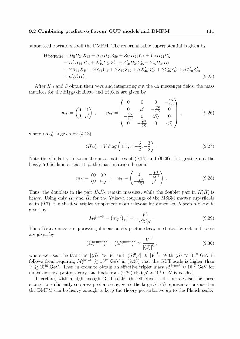
9.2 Combining predictive flavour GUT models and DMPM 111
suppressed operators spoil the DMPM. The renormalisable superpotential is given by
WDMPM24 = H5H24X45 + X45H24Z50 + Z50H24Y45 + Y45H24H′5
+ H ′5H24X′45 + X ′45H24Z
′50 + Z ′50H24Y
′45 + Y ′45H24H5
+ SX45X45 + SY45Y45 + SZ50Z50 + SX ′45X′45 + SY ′45Y
′45 + SZ ′50Z
′50
+ µ′H ′5H′5 . (9.25)
After H24 and S obtain their vevs and integrating out the 45 messenger fields, the massmatrices for the Higgs doublets and triplets are given by
mD =
(0 00 µ′
), mT =
0 0 0 − V 2
〈S〉0 µ′ − V 2
〈S〉 0
− V 2
〈S〉 0 〈S〉 0
0 − V 2
〈S〉 0 〈S〉
, (9.26)
where 〈H24〉 is given by (4.13)
〈H24〉 = V diag
(1, 1, 1,−3
2,−3
2
). (9.27)
Note the similarity between the mass matrices of (9.16) and (9.26). Integrating out theheavy 50 fields in a next step, the mass matrices become
mD =
(0 00 µ′
), mT =
(0 − V 4
〈S〉3
− V 4
〈S〉3 µ′
). (9.28)
Thus, the doublets in the pair H5H5 remain massless, while the doublet pair in H ′5H′5 is
heavy. Using only H5 and H5 for the Yukawa couplings of the MSSM matter superfieldsas in (9.7), the effective triplet component mass relevant for dimension 5 proton decay isgiven by
Mdim=5T =
(m−1T
)−1
11= − V 8
〈S〉6µ′ . (9.29)
The effective masses suppressing dimension six proton decay mediated by colour tripletsare given by (
Mdim=6T
)2=(Mdim=6
T
)2 ≈ |V |8
|〈S〉|6, (9.30)
where we used the fact that |〈S〉| |V | and |〈S〉3µ′| |V |4. With 〈S〉 ≈ 1018 GeV itfollows from requiring Mdim=6
T & 1012 GeV in (9.30) that the GUT scale is higher thanV & 1016 GeV. Then in order to obtain an effective triplet mass Mdim=5
T ≈ 1017 GeV fordimension five proton decay, one finds from (9.29) that µ′ ≈ 107 GeV is needed.
Therefore, with a high enough GUT scale, the effective triplet masses can be largeenough to sufficiently suppress proton decay, while the large SU(5) representations used inthe DMPM can be heavy enough to keep the theory perturbative up to the Planck scale.

112 9. Towards predictive SUSY flavour SU(5) models with DT splitting
Let us note two remarks: When H24 is uncharged under additional symmetries, havingµ′ several orders of magnitude smaller than V requires µ′ to be generated from vevs offields charged under the shaping symmetry, to forbid the term
H24H′5H′5 , (9.31)
which would give rise to a much too small effective triplet mass.Finally note that the effective triplet mass entering dimension five proton decay can be
conveniently expressed in terms of the mass eigenstates M1 and M2 of the triplet compo-nents and µ′ of the doublets
Mdim=5T = −M1M2
µ′. (9.32)
The effective triplet mass of dimension six proton decay is then excellently approximatedby
Mdim=6T = Mdim=6
T ≈√Mdim=5
T µ′ . (9.33)
9.2.3 Introducing a second adjoint
The DMPM with an adjoint GUT breaking Higgs instead of a 75 already solves the DTSproblem while providing the necessary building block for the desirable CG factors forflavour model building, if the GUT scale is high enough. Yet, it still suffers from twoproblems:
Gauge coupling unification As mentioned in 5.5, demanding gauge coupling unifica-tion in the minimal renormalisable SU(5) requires the mass of the colour triplets to beabout 1015 GeV, which violates the bounds on proton decay. Non-renormalisable operatorsin the GUT breaking superpotential can split the 24 component masses, allowing a highereffective triplet mass [146], at the price of giving up the predictive quark-lepton Yukawacoupling ratios.
Shaping symmetry charge of the adjoint The renormalisable superpotential (5.83)requires H24 to be uncharged under shaping symmetries in order for it to obtain a vev.However, such a shaping symmetry charge is vital in the type of flavour models consideredhere, to avoid unwanted admixtures of additional CG factors involving less insertions ofH24. See for example the SUSY flavour GUT models in the previous chapters and tablesD.1 and D.3.
Both problems can be solved at once by introducing a second adjoint superfield:
• An additional heavy 24 can be used to UV complete a non-renormalisable superpotential,thereby realising a renormalisable theory which shifts the upper bound for the effectivetriplet mass to higher values (5.90), by splitting the masses of the 24 components.

9.2 Combining predictive flavour GUT models and DMPM 113
• It turns out that the introduction of an additional 24 is not just an UV-completion ofthe non-renormalisable superpotential of [146]. When both adjoints have approximatelythe same mass and therefore the second 24 is not integrated out, the additional colouroctet and electroweak triplet in the spectrum lead to more freedom for the GUT scaleand effective triplet masses.
• Finally, with a second 24, the adjoint fields can acquire non-vanishing vevs even whencharged under shaping symmetries.
There are four possibilities for renormalisable superpotentials of two adjoints with non-vanishing vevs and masses. Classified based on their symmetry, they are:
(a) W = M24 Tr H224 +M ′
24Tr H ′224 + κ′Tr H24H′224 + λTr H3
24,Z2 symmetry where H24 is uncharged and H ′24 charged.
(b) W = M24 Tr H24H′24 + λTr H3
24 + λ′Tr H ′324,Z3 symmetry, where H24 has charge 2 and H ′24 charge 1.
(c) W = M24 Tr H24H′24 + λTr H3
24 + κ′Tr H24H′224,
ZR4 symmetry where H24 has a charge of 2 (with R(θ) = 1) and H ′24 is uncharged.
(d) The trivial case with both fields only charged under SU(5) and all (non-linear) termsallowed. We will not consider this case any further.
Let us remark that since the superpotentials (a), (b), and (d) do not feature an R-symmetry and superpotential (c) spontaneously breaks the R-symmetry simultaneouslywith the GUT gauge group, all four superpotentials are not in conflict with the No-Gotheorem that the MSSM with an additional unbroken R-symmetry can not be obtainedfrom the spontaneous breaking of a four-dimensional SUSY GUT [186].
9.2.4 The case of more Higgs fields coupling to matter
Consider the SUSY flavour GUT models of the previous chapters, where an additionalHiggs field H45 transforming as 45 under SU(5) was introduced in order to construct theCG factor −1
2. In 9.1 we have so far only considered the case where a single pair of Higgs
fields H5, H5 couples to the matter superfields. Let us now discuss the case where morethan one Higgs triplet is coupling to matter.
With additional Higgs fields (9.7) generalises to
W = κijaTiTjHa + λijbTiFjHb +mHabHaHb , (9.34)
where a and b denote different Higgs fields, κ and λ are Yukawa couplings, and mH is theHiggs mass matrix. When the heavy triplets are integrated out, the proton decay channels
κijaλklb(Mdim=5
T
)ba
(Qi ·Qj) (Qk · Ll) andκijaλklb(Mdim=5
T
)ba
U ciE
cjU
ckD
cl (9.35)

114 9. Towards predictive SUSY flavour SU(5) models with DT splitting
are suppressed by the effective triplet mass
(Mdim=5T )−1
ba ≡ U∗ai
(mdiagT
)−1
ijVbj = U∗ai
(mdiagT
)−1
ijV Tjb = (m−1
T )ba , (9.36)
with mT being the mass matrix of the coloured triplets in Ha, Hb. Similarly, the Kahlerpotential in general reads
KT = TaT∗a + TaT
∗a . (9.37)
When the heavy Higgs triplets are integrated out, baryon number violating operatorsemerge in the Kahler potential
|κija|2(Mdim=6
T
)2
aa
(Qi ·Qj)Uc∗i E
c∗j and
|λija|2(Mdim=6
T
)2
aa
(Qi · Lj)U c∗i D
c∗j , (9.38)
where no sum over i, j, and a is implied. The dimension six effective triplet masses arethen in general given by(
Mdim=6T
)−2
aa≡ Vai
(mdiagT
)−1
ijU †jbUbm
(mdiagT
)−1
mlV †la =
(m−1T m†−1
T
)aa
(9.39)
and (Mdim=6
T
)−2
aa≡(m†−1T m−1
T
)aa. (9.40)
Thus, in models featuring several Higgs fields coupling to specific matter fields, as e.g. toconstruct predictions for quark-lepton Yukawa coupling ratios from certain CG factors, theindividual effective triplet masses for each proton decay channel can be easily calculated.
9.3 Grand unification and the effective triplet mass
In addition to the MSSM superfields, the DMPM introduces one extra pair of SU(2)Ldoublets, D(5) and D(5), and two additional pairs of SU(3)C triplets, T
(5)i and T
(5)i , i = 1, 2.
Since we introduce a second adjoint, there are furthermore two SU(3)C octets O(24)i , two
SU(2)L triplet T(24)i , and two singlets S
(24)i of the SM gauge group, when SU(5) gets
broken. Finally there is one leptoquark superfield pair L(24) in the spectrum, whereas theother pair yields massive X and Y vector bosons via the BEH mechanism.
All this new superfields enter the RGEs for the gauge couplings at their respective massscales and therefore their impact on gauge coupling unification has to be studied. Such ananalysis has been performed by the author’s collaborator Vinzenz Maurer. Thus, in thisthesis only some results – which are important to the author’s work presented afterwards– are briefly reviewed in this section. Details can be found in our paper [4] and VinzenzMaurer’s PhD thesis [158].
We assume that the heaviest incomplete SU(5) multiplets to enter the RGEs are the Xand Y vector bosons, such that the GUT scale corresponds to their heavy mass MGUT =

9.3 Grand unification and the effective triplet mass 115
MX = MY . This is a common situation in SU(5) GUTs and it allows to make the effectivetriplet mass heavy, although cases of other heaviest SU(5) components are possible.
With the definition of the geometric mean
M2T (5) ≡M
T(5)1M
T(5)2
(9.41)
of the masses of the colour triplets and analogously
M2T (24) ≡M
T(24)1
MT
(24)2
, (9.42)
M2O(24) ≡M
O(24)1M
O(24)2
(9.43)
for the masses of the components of H24 and H ′24, one can solve the RGEs for gaugecoupling unification and express the results for the effective triplet mass (9.32)
Mdim=5T =
M2T (5)
MD(5)
, (9.44)
the GUT scale SU(5) gauge coupling αu, and MGUT at the one-loop level by
πα−1u = − 43π
24α1
+15π
8α2
+11π
12α3
− 197
20logMZ +
3
5logMDT (9.45)
− 3
4logML(24) +
15
4logMT (24) +
11
4logMO(24) +
7
2logMSUSY ,
logMdim=5T = − 5π
6α1
+5π
2α2
− 5π
3α3
+1
6logMZ (9.46)
+ 5 logMT (24) − 5 logMO(24) +5
6logMSUSY ,
logMGUT =5π
12α1
− π
4α2
− π
6α3
+11
6logMZ (9.47)
+1
2logML(24) − 1
2logMT (24) − 1
2logMO(24) − 1
3logMSUSY ,
where “logm” should be understood as
logm ≡ log( m
GeV
)(9.48)
and we have introduced the mass
M3DT ≡M2
D(5)MT (5) . (9.49)
Then one finds numerically
Mdim=5T = 2.5+0.6
−0.8 · 1017 GeV
(MSUSY
1 TeV
) 56(MT (24)
MO(24)
)5
, (9.50)
MGUT = 1.37+0.05−0.05 · 1016 GeV
(MSUSY
1 TeV
)− 13(
ML(24)
1016 GeV
) 12(MT (24)MO(24)
(1016 GeV)2
)− 12
, (9.51)

116 9. Towards predictive SUSY flavour SU(5) models with DT splitting
where the resulting uncertainty is dominated by the experimental error on αs. The changeof the relative uncertainty for the different superpotentials (a)-(c) is negligible and hencein the remainder of this section the error is not explicitly shown anymore.
In analogy to tan β of the MSSM, we introduce tan βV = V1
V2for the two GUT breaking
superfields H24 and H ′24 with
〈H24〉 = V1 eiφ1 diag(1, 1, 1,−3/2,−3/2) ,
〈H ′24〉 = V2 eiφ2 diag(1, 1, 1,−3/2,−3/2) , (9.52)
where V1, V2 > 0.Then one finds for the geometric means of the masses of the colour triplets, octets, and
the mass of the remaining leptoquark superfield in H24 and H ′24
M2T (24) =
35
4M2 , M2
O(24) =15
4M2 , and M2
L(24) =1
sin2(2βV )M2 , (9.53)
for superpotential (b) and
M2T (24) =
5
4M2 , M2
O(24) =5
4M2 , and M2
L(24) =1
4 sin2(2βV )M2 , (9.54)
for superpotential (c), where M ≡∣∣∣M24
∣∣∣, i.e. in both cases all mass eigenvalues turn out
to be phase independent. The effective triplet mass is then obtained from (9.50)
Mdim=5, 1-loopT = 2.5 · 1017 GeV
(MSUSY
1 TeV
) 56
×(
73
) 52 ≈ 8.3 (b)
1 (c), (9.55)
and the GUT scale from (9.51)
M1-loopGUT =
1.37 · 1016 GeV√| sin 2βV |
(MSUSY
1 TeV
)− 13(
M
1015 GeV
)− 12
×√
8√21≈ 1.32 (b)
2 (c). (9.56)
Thus, assuming the same parameters, the effective triplet mass in superpotential (b) is tentimes higher than in (c).
The effective triplet mass Mdim=5T receives significant two-loop contributions (cf. e.g.
[145]). See our paper [4] and [158] for a numerical two-loop analysis. Its results are givenby
Mdim=5, 2-loopT =
(MSUSY
1 TeV
)0.74
·
5.2 · 1016 GeV(
M1015 GeV
)−0.15(b)
6.8 · 1015 GeV(
M1015 GeV
)−0.18(c)
, (9.57)
and
M2-loopGUT = |sin 2βV |−0.48
(MSUSY
1 TeV
)−0.4
·
2.89 · 1016 GeV(
M1015 GeV
)−0.61(b)
4.78 · 1016 GeV(
M1015 GeV
)−0.63(c)
, (9.58)

9.4 SUSY Flavour GUT models with DMPM 117
where MD(5) = 1000 TeV has been fixed and the dependence on other parameters is verysmall. Thus, a heavy effective triplet mass Mdim=5
T & 1017 GeV requires MSUSY & 2.3 TeVand 35 TeV for superpotential (b) and (c), respectively.
Note that gauge coupling unification depends only weakly on MD(5) . The effective tripletmass for dimension six proton decay can be approximated by (9.33) from the square rootof the product of MD(5) and Mdim=5, 1-loop
T or Mdim=5, 2-loopT respectively.
Finally we turn to superpotential (a), which is more complicated since it contains twomass parameters M24 and M ′
24. Thus we introduce a second angle βM and mean massM > 0 such that M24 = Meiα1 sin βM and M ′
24 = Meiα2 cos βM . Then the geometricmean masses of the SU(3)C octet, SU(2)L triplet, and of the additional heavy leptoquarksuperfields are
M2T (24) = 5M2 cos βM
√(2 cos βM − 3 sin βM tan2 βV )2 + . . . sin2 φ , (9.59a)
M2O(24) = 5M2 cos βM
√(3 cos βM − 2 sin βM tan2 βV )2 + . . . sin2 φ , (9.59b)
M2L(24) =
1
4M2 cos2 βM
sin4 βV, (9.59c)
where not only the geometric mean masses, but also the mass eigenvalues themselves, onlydepend on the phase combination
φ ≡ (α1 − α2)/2 + φ1 − φ2 , (9.60)
and are invariant under φ→ φ+π. Due to (9.50), the effective triplet mass is heaviest when
the ratioMT (24)
MO(24)
is not bounded from above, and hence when φ is 0, π, or 2π. In figure 9.3
the resulting plots for Mdim=5T and MGUT are shown with MSUSY = 1 TeV, M = 1015 GeV,
MD(5) = 1000 TeV, and φ = 0, including a comparison between one- and two-loop results.Mdim=6
T and Mdim=6T
are again approximately given by√Mdim=5
T MD(5) .
9.4 SUSY Flavour GUT models with DMPM
After the interlude of the last section, we return to the author’s contribution to [4] andpresent two example models, combining the DMPM (featuring two adjoint superfields)and predicitive GUT scale quark-lepton Yukawa coupling ratios due to CG factors. Bothmodels are UV complete and we give the shaping symmetries and messenger superfields,which guarantee that only the desired effective GUT operators are generated when theheavy degrees of freedom are integrated out.
Note that we construct only the Yukawa matrices of the quarks and charged leptonsexplicitly. Adding one of the ubiquitous mechanisms to generate neutrino masses andlepton mixing angles would be straightforward. Since they are however not directly relevantfor the discussion of proton decay, doublet-triplet splitting, and the CG factors betweenYd and Ye, we do not consider neutrinos in this chapter.

118 9. Towards predictive SUSY flavour SU(5) models with DT splitting
Mdim=5T
0.6 0.8 1.0 1.2 1.4 1.6
0.8
1.0
1.2
1.4
1.6
1.8
2.0
M24
¢ M24
V2
V
1
1016
1017
1018
1019
-6-4-20246
0.6 0.8 1.0 1.2 1.4 1.6
0.8
1.0
1.2
1.4
1.6
1.8
2.0
M24
¢ M24
V2
V
1
1016
1017
1018
1019
-6-4-20246
MGUT
0.6 0.8 1.0 1.2 1.4 1.6
0.8
1.0
1.2
1.4
1.6
1.8
2.0
M24
¢ M24
V2
V
1
2×10¹⁶
3×10¹⁶
5×10¹⁶
7×10¹⁶
-6-4-20246
0.6 0.8 1.0 1.2 1.4 1.6
0.8
1.0
1.2
1.4
1.6
1.8
2.0
M24
¢ M24
V2
V
1
2×10¹⁶
3×10¹⁶
5×10¹⁶
7×10¹⁶
-6-4-20246
Figure 9.3: The effective colour triplet mass Mdim=5T (left) and GUT scale MGUT (right)
in GeV at one-loop (upper) and two-loop (lower) order as resulting from superpotential (a)for MSUSY = 1 TeV, M = 1015 GeV, MD(5) = 1000 TeV, and φ = 0. Note the differentcolour coding between left and right. For illustration, the white strips denote areas withlight MT (24) or MO(24) (< 1013 GeV). Such relatively low values for these components canarise either from cancellation between terms, or from a generic suppression due to smallparameters, cf. (9.59). For more details see [4, 158].

9.4 SUSY Flavour GUT models with DMPM 119
We also remark, that our two models are not yet predictive for the quark mixing param-eters, but the experimentally observed values can be fitted by both of the models. Theythus should be viewed as proof of existence, showing that a successful solution to DTSand experimentally viable predictions for GUT scale Yukawa coupling ratios can indeed becombined. The strategies discussed here, however, provide the tools for the constructionof more ambitious SUSY flavour GUT models, which should include the observed neutrinomasses and finally also predict the quark and lepton mixing angles and CP phases.
Thus there are two types of predictions our example models make: As discussed in 4.4,in general one can directly constrain GUT models from their GUT scale double ratio (4.43)∣∣∣∣yµys ydye
∣∣∣∣ , (9.61)
which as mentioned previously is not affected by RG evolution or SUSY threshold cor-rections. As for the SUSY flavour GUT models of the previous chapters, we will againuse the CG factors yτ
yb= −3
2, yµys
= 6, and yeyd
= −12
in agreement with (4.43), whereasthe ubiquitous GJ relations are challenged with more than two sigma deviation from theexperimental value.
Secondly, the predictions for the Yukawa coupling ratios at the GUT scale imply – viaSUSY threshold corrections – constraints on the SUSY breaking parameters, which may betested at future collider searches if SUSY is discovered. See e.g. [187] for a discussion andan explicit example of such constraints. We will discuss this link between GUT predictionsand SUSY spectrum in general in chapter 10.
Our two examples will feature different Yukawa matrix structures. In the first modelwe construct diagonal down-type quark and charged lepton Yukawa matrices Yd and Ye,with all quark mixing originating from the up-type quark Yukawa matrix Yu. Then, in thesecond model we realise the attractive feature of θC originating from Yd.
9.4.1 A model with diagonal Yd and Ye Yukawa matrices
We now turn to our first model featuring diagonal down-type quark and charged leptonYukawa matrices Yd and Ye in the flavour basis. An approach to flavour (GUT) modelbuilding with diagonal Ye (and Yd) has been discussed in [188]. In this case all the mixingin the quark sector has to come exclusively from the up-type quark Yukawa matrix Yu.Explicitly, our model has the following structure for the Yukawa matrices
Yd =
yd 0 00 ys 00 0 yb
, Ye =
−12yd 0 0
0 6ys 00 0 −3
2yb
, Yu =
y11 y12 y13
y12 y22 y23
y13 y23 y33
. (9.62)
We introduce flavon superfields θ1, θ2, θ3, and θ4 that obtain a vev and generate thehierarchical structure of the Yukawa matrices. After the flavons and the GUT breakingH24 and H ′24 obtain their vevs, the Yukawa matrices (9.62) originate from the effective
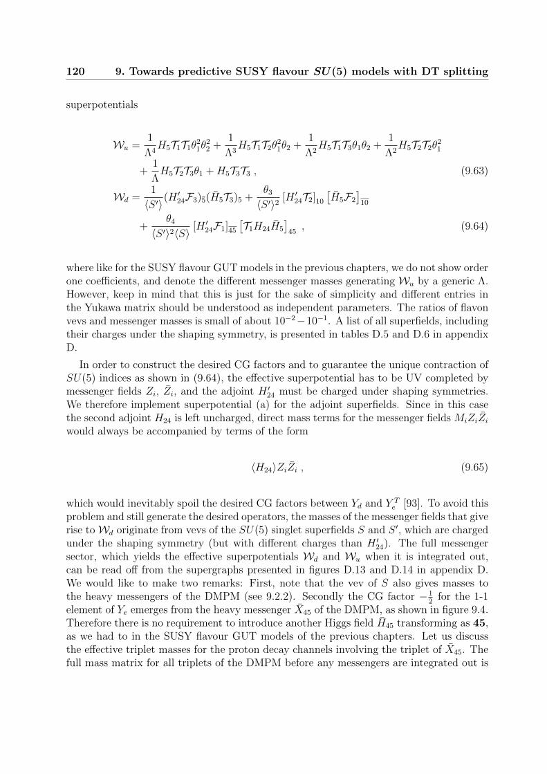
120 9. Towards predictive SUSY flavour SU(5) models with DT splitting
superpotentials
Wu =1
Λ4H5T1T1θ
21θ
22 +
1
Λ3H5T1T2θ
21θ2 +
1
Λ2H5T1T3θ1θ2 +
1
Λ2H5T2T2θ
21
+1
ΛH5T2T3θ1 +H5T3T3 , (9.63)
Wd =1
〈S ′〉(H′24F3)5(H5T3)5 +
θ3
〈S ′〉2 [H ′24T2]10
[H5F2
]10
+θ4
〈S ′〉2〈S〉 [H ′24F1]45
[T1H24H5
]45, (9.64)
where like for the SUSY flavour GUT models in the previous chapters, we do not show orderone coefficients, and denote the different messenger masses generating Wu by a generic Λ.However, keep in mind that this is just for the sake of simplicity and different entries inthe Yukawa matrix should be understood as independent parameters. The ratios of flavonvevs and messenger masses is small of about 10−2−10−1. A list of all superfields, includingtheir charges under the shaping symmetry, is presented in tables D.5 and D.6 in appendixD.
In order to construct the desired CG factors and to guarantee the unique contraction ofSU(5) indices as shown in (9.64), the effective superpotential has to be UV completed bymessenger fields Zi, Zi, and the adjoint H ′24 must be charged under shaping symmetries.We therefore implement superpotential (a) for the adjoint superfields. Since in this casethe second adjoint H24 is left uncharged, direct mass terms for the messenger fields MiZiZiwould always be accompanied by terms of the form
〈H24〉ZiZi , (9.65)
which would inevitably spoil the desired CG factors between Yd and Y Te [93]. To avoid this
problem and still generate the desired operators, the masses of the messenger fields that giverise toWd originate from vevs of the SU(5) singlet superfields S and S ′, which are chargedunder the shaping symmetry (but with different charges than H ′24). The full messengersector, which yields the effective superpotentials Wd and Wu when it is integrated out,can be read off from the supergraphs presented in figures D.13 and D.14 in appendix D.We would like to make two remarks: First, note that the vev of S also gives masses tothe heavy messengers of the DMPM (see 9.2.2). Secondly the CG factor −1
2for the 1-1
element of Ye emerges from the heavy messenger X45 of the DMPM, as shown in figure 9.4.Therefore there is no requirement to introduce another Higgs field H45 transforming as 45,as we had to in the SUSY flavour GUT models of the previous chapters. Let us discussthe effective triplet masses for the proton decay channels involving the triplet of X45. Thefull mass matrix for all triplets of the DMPM before any messengers are integrated out is

9.4 SUSY Flavour GUT models with DMPM 121
H ′24
H24
H5
Z45,1Z45,1
F1
Z45,2 Z45,2
θ4
X45X45
T1
〈S〉〈S′〉 〈S′〉
Figure 9.4: Supergraph leading to ye = −12yd when the heavy messenger fields are inte-
grated out.
given by
mT =
H5 H′5 X45 Y45 Z50 X′45 Y ′45 Z′50
H5 0 0 0 0 0 0 V1 0H′5 0 µ′ 0 V1 0 0 0 0X45 V1 0 〈S〉 0 0 0 0 0Y45 0 0 0 〈S〉 V1 0 0 0Z50 0 0 V1 0 〈S〉 0 0 0X′45 0 V1 0 0 0 〈S〉 0 0Y ′45 0 0 0 0 0 0 〈S〉 V1
Z′50 0 0 0 0 0 V1 0 〈S〉
, (9.66)
where V1 is defined in (9.52) and we have annotated the rows and columns for a betteroverview. The proton decay mediated by the triplet pair in H5 and X45 is then suppressedby the effective triplet mass (9.36)(
Mdim=5T
)31
=(m−1T
)−1
31= − V 7
1
〈S〉5µ′ , (9.67)
which is about two orders of magnitude larger than the effective triplet mass associatedwith proton decay mediated by the triplets in H5 and H5 (9.29)(
Mdim=5T
)11
= − V 81
〈S〉6µ′ . (9.68)
Also the dimension six proton decay mediated by the triplets in X45 (9.40)
(Mdim=6
T
)2
33≈ |V1|6
|〈S〉|4, (9.69)
is approximately four orders of magnitude larger than (9.30)
(Mdim=6
T
)2
11≈ |V1|8
|〈S〉|6. (9.70)
It is thus sufficient to limit our discussion to the effective triplet masses of proton decaymediated by the triplets in H5 and H5.

122 9. Towards predictive SUSY flavour SU(5) models with DT splitting
Finally note that the additional colour triplets of all DMPM messengers, H ′5, and H ′5can couple to the matter superfields only via effective operators, which can contribute toproton decay but are suppressed compared to the leading operators by one or more powers
of H24
Mpland
H′24
Mpl. Their contribution can thus safely be neglected.
Let us now comment on the phenomenology of Yd and Yu. The hierarchical structure ofYd is enforced due to the use of higher order effective operators in Wd. The eigenvalues ofYu and the mixing angles are given in leading order in a small angle approximations as
yu ≈ y11 −y2
12
y22
, yc ≈ y22 , yt ≈ y33 , θC ≈y12
y22
, θ23 ≈y23
y33
, θ13 ≈y13
y33
. (9.71)
Phenomenology requires that all parameters yij of Yu are independent, which needs to becarefully considered in the construction of the messenger sector. When we present themessenger sector in appendix D we also discuss that a similar choice of messenger fields,which generates the same structure (9.62) for the Yukawa matrices and thus would seemas an equally viable choice, in fact predicts invalid dependencies between the quark mixingangles.
We argued in 9.2.2 that for the case of an uncharged H24, as it appears in the selectedsuperpotential (a) for our model, the mass term for the additional Higgs fields H ′5H
′5 must
come from the vev of some singlet field. In our model an effective µ′ term is generatedfrom a higher-dimensional operator and with an even higher suppression, there is also aµ-term for the Higgs fields coupling to matter
Weff5 = µH5H5 + µ′H ′5H
′5 , (9.72)
where
µ′ ≡ 〈θ3〉4M3
pl
and µ ≡ 〈θ3〉〈θ4〉4M4
pl
. (9.73)
Alternatively, we checked that an UV-complete generation of these µ and µ′ operatorsvia messenger fields would be possible. However, the necessary messenger fields are notincluded in the model since it turns out that the desired masses are already generated byPlanck scale suppressed effective operators.
Integrating out the heavy 45 and 50 messengers and after SU(5) gets spontaneouslybroken, the effective triplet mass for dimension five proton decay is given by (9.29)
Mdim=5T = µ− V 8
1
〈S〉6µ′ ≈ −V 8
1 M3Pl
〈S〉6〈θ3〉4, (9.74)
and the effective triplet masses suppressing dimension six proton decay by (9.30)
Mdim=6T = Mdim=6
T ≈ V 41
〈S〉3 . (9.75)
Let us give an explicit example for the scales involved in the model: Because of pertur-bativity the mass of the 50 messengers has to be almost at the Planck scale. We thereforeassume
〈S〉 ∼ 10−1Mpl . (9.76)
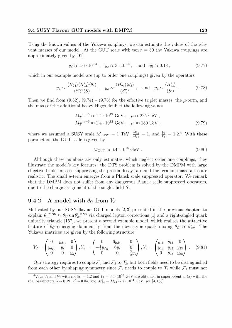
9.4 SUSY Flavour GUT models with DMPM 123
Using the known values of the Yukawa couplings, we can estimate the values of the rele-vant masses of our model. At the GUT scale with tan β = 30 the Yukawa couplings areapproximately given by [91]
yd ≈ 1.6 · 10−4 , ys ≈ 3 · 10−3 , and yb ≈ 0.18 , (9.77)
which in our example model are (up to order one couplings) given by the operators
yd ∼〈H24〉〈H ′24〉〈θ4〉〈S ′〉2〈S〉 , ys ∼
〈H ′24〉〈θ3〉〈S ′〉2 , and yb ∼
〈H ′24〉〈S ′〉 . (9.78)
Then we find from (9.52), (9.74) – (9.78) for the effective triplet masses, the µ-term, andthe mass of the additional heavy Higgs doublet the following values
Mdim=5T ≈ 1.4 · 1019 GeV , µ ≈ 225 GeV ,
Mdim=6T ≈ 1.4 · 1012 GeV , µ′ ≈ 130 TeV , (9.79)
where we assumed a SUSY scale MSUSY = 1 TeV,M ′24
M24= 1, and V2
V1= 1.2.4 With these
parameters, the GUT scale is given by
MGUT ≈ 6.4 · 1016 GeV . (9.80)
Although these numbers are only estimates, which neglect order one couplings, theyillustrate the model’s key features: the DTS problem is solved by the DMPM with largeeffective triplet masses suppressing the proton decay rate and the fermion mass ratios arerealistic. The small µ-term emerges from a Planck scale suppressed operator. We remarkthat the DMPM does not suffer from any dangerous Planck scale suppressed operators,due to the charge assignment of the singlet field S.
9.4.2 A model with θC from Yd
Motivated by our SUSY flavour GUT models [2, 3] presented in the previous chapters toexplain θPMNS
13 ≈ θC sin θPMNS23 via charged lepton corrections [1] and a right-angled quark
unitarity triangle [157], we present a second example model, which realises the attractivefeature of θC emerging dominantly from the down-type quark mixing θC ≈ θd12. TheYukawa matrices are given by the following structure
Yd =
0 yd12 0yd21 ys 00 0 yb
, Ye =
0 6yd21 0−1
2yd12 6ys 00 0 −3
2yb
, Yu =
y11 y12 0y12 y22 y23
0 y23 y33
. (9.81)
Our strategy requires to couple F1 and F2 to T2, but both fields need to be distinguishedfrom each other by shaping symmetry since F2 needs to couple to T1 while F1 must not
4Vevs V1 and V2 with cotβV = 1.2 and V1 = 3.4 · 1016 GeV are obtained in superpotential (a) with thereal parameters λ ∼ 0.19, κ′ ∼ 0.04, and M ′24 = M24 ∼ 7 · 1014 GeV, see [4, 158].

124 9. Towards predictive SUSY flavour SU(5) models with DT splitting
couple to T1. This suggests to employ at least a Z3 shaping symmetry and we thereforeuse superpotential (b) from section 9.2.3, where H24 and H ′24 are charged.
The effective superpotentials that yield the desired Yukawa matrices after integratingout heavy messenger fields and breaking of the GUT gauge group are
Wu =1
Λ2H5T1T1θ
25 +
1
Λ2H5T1T2θ
22 +
1
Λ2H5T2T2θ
21 +
1
ΛH5T2T3θ1 +H5T3T3 , (9.82)
Wd =1
〈S ′〉(H′24F3)5(H5T3)5 +
θ3
〈S ′〉2 (H24T2)10(H5F1)10 +θ4
〈S ′〉2 (H ′24T2)10(H5F2)10
+1
〈S〉2 (H24F2)45(T1H24H5)45 , (9.83)
where again we use a common placeholder Λ to denote a generic messenger mass and themessenger fields responsible for Wd obtain their masses from vevs of singlet fields. Notethat in comparison to Yu of the previous example model (9.62), the vanishing Yu13 elementrequires to introduce an additional flavon field θ5.
The supergraphs that generate these effective operators are shown in figures D.15 andD.16 in appendix D. A complete list of all superfields including their charges and rep-resentations is given in tables D.7 and D.8. Note that again we do not introduce a newHiggs field H45 that couples to matter superfields, but the CG factor −1
2emerges from the
DMPM messenger X45, see figure 9.5. Analogously to the discussion below figure 9.4, it is
H24
H24
H5
Z45,1Z45,1
F2
X45X45
T1
〈S〉〈S〉
Figure 9.5: Supergraph yielding the CG factor −12 when the heavy messenger fields are
integrated out.
sufficient to limit our discussion to the effective triplet masses of proton decay mediated bythe triplet pair in H5 and H5, since the effective triplet mass of the X45 decay channel isorders of magnitude higher. Other effective operators coupling matter superfields to other
triplets of the DMPM are again sufficiently suppressed by powers of M24
Mpl.
In a small angle approximation the mixing angles and Yukawa couplings are given by
yd ≈yd12yd21
ys, θC ≈ θd12 ≈
yd12
ys,
yu ≈ y11 −y2
12
y22
, yc ≈ y22 , yt ≈ y33 , θ23 ≈y23
y33
, θ13 ≈y12
y22
θ23 , (9.84)
and in leading order the strange and bottom quark Yukawa couplings are given by theparameters ys and yb of Yd in (9.81). Thus the Yukawa matrices can fit the experimentalvalues without tension.

9.4 SUSY Flavour GUT models with DMPM 125
Let us now discuss the DMPM details of the model. As in 9.4.1, the mass terms ofthe Higgs fields H5H5 and H ′5H
′5 are generated from Planck suppressed effective operators
(9.72) with
µ ≡ 〈θ3〉4M3
pl
and µ′ ≡ 〈θ4〉4M3
pl
. (9.85)
Although µ and µ′ appear at the same order, a modest hierarchy 〈θ3〉 < 〈θ4〉 sufficientlysplits their masses. We will see below that indeed such a slight hierarchy is realised in ourmodel.
The effective triplet masses (9.29) and (9.30) are given by
Mdim=5T = µ− V 8
1
〈S〉6µ′ ≈ −V 8
1 M3Pl
〈S〉6〈θ4〉4, (9.86)
Mdim=6T = Mdim=6
T ≈ V 41
〈S〉3 . (9.87)
As for the first example model we can estimate the values of the relevant masses in anexplicit example from the known Yukawa couplings [91]. In a small angle approximationthe down-type Yukawa couplings are given by
yd ∼〈H24〉2〈S〉2
〈H24〉〈θ3〉〈S ′〉2
1
ys≈ 1.6 · 10−4 with ys ∼
〈H ′24〉〈θ4〉〈S ′〉2 ≈ 3 · 10−3 (9.88)
and
yb ∼〈H ′24〉〈S ′〉 ≈ 0.18 , (9.89)
where the numerical values are valid for tan β = 30 and again order one coefficients havebeen neglected. Again, because of perturbativity we assume 〈S〉 = 10−1 Mpl. Then thenumerical values of the effective triplet masses, µ, and µ′ can be estimated
Mdim=5T ≈ 1.4 · 1018 GeV , Mdim=6
T ≈ 1012 GeV , µ ≈ 7 TeV , µ′ ≈ 800 TeV , (9.90)
where we assumed tan βV = 12.5 Note the solutions for 〈θ3〉 and 〈θ4〉, which are
〈θ3〉 ≈ 2 · 1015 GeV and 〈θ4〉 ≈ 6 · 1015 GeV , (9.91)
whose slight splitting explains the huge hierarchy between µ and µ′, as mentioned above.We also find
MSUSY ≈ 26 TeV and MGUT ≈ 3.4 · 1017 GeV . (9.92)
Also in our second model we thus successfully suppress proton decay via large effectivetriplet masses, where the DTS is achieved via the DMPM with two adjoints. The Yukawasector of the model features viable fermion masses and mixing angles. A small µ-term forthe Higgs doublets emerges from Planck suppressed effective operators.
5In superpotential (b) this tanβV can be obtained with V1 = 3.2 · 1016 GeV from real parametersλ ∼ 10−4, λ′ ∼ 1.3 · 10−5, and M ∼ 2.4 · 1012 GeV, see [4, 158].

126 9. Towards predictive SUSY flavour SU(5) models with DT splitting
9.5 Proton Decay
We now turn to a discussion of proton decay and start by discussing the dimension fiveoperators (5.85)
WT = (YqlQ · L− YudU cDc) T (5) + (YueUcEc − YqqQ ·Q)T (5) , (9.93)
which are usually considered to be the greatest danger for the validity of any SUSY GUTmodel. To suppress proton decay sufficiently, the colour triplets have to be very heavy ortheir couplings to the matter fields should be very strongly suppressed.
Minimal SU(5) models lead to wrong predictions for the quark-lepton mass ratios. Inmany models it is thus assumed that non-renormalisable operators resolve this problem,at least for the first two generations, as for example [146,189]. In such settings the modelloses predictability and usually it is impossible to calculate the strength of the couplingbetween matter fields and Higgs triplets.6
In our method viable GUT scale quark-lepton mass ratios are predicted by new CGfactors due to specific effective operators, which are uniquely obtained by integrating outa distinct set of messenger fields charged under a shaping symmetry. With the sametechnique also the GUT scale Yukawa couplings to Higgs triplets are predicted from group-theoretical CG factors. These CG factors for the triplet Yukawa couplings have beencalculated by the author’s collaborateur Vinzenz Maurer from dimension five and dimensionsix operators containing one or two adjoints [4, 158]. The CG factors used in our modelsare listed in figure 9.6.
Then the Yukawa matrices of our first model 9.4.1 are given by
Yd = diag (yd, ys, yb) , Ye = diag
(−1
2yd, 6ys,−
3
2yb
), (9.94)
Yql = diag
(yd, ys,−
3
2yb
), Yud = diag
(2
3yd,−4ys, yb
), (9.95)
Yqq =1
2Yu , Yue = Yu , (9.96)
where the structure of Yu can be read off from (9.62). For the second model 9.4.2 we find
Yd =
0 yd,12 0yd,21 ys 0
0 0 yb
, Y Te =
0 −12yd,12 0
6yd,21 6ys 00 0 −3
2yb
, (9.97)
Yql =
0 yd,12 0yd,21 ys 0
0 0 −32yb
, Yud =
0 23yd,12 0
−4yd,21 −4ys 00 0 yb
, (9.98)
Yqq =1
2Yu , Yue = Yu , (9.99)
6GUT textures for proton decay, without fully constructed models, have been considered, for example,in [190].

9.5 Proton Decay 127
A
B
C
D
R R
A
B
CD
E
R2R2R1R1
Dimension five operators
AB C D R (Yd)ij : (Ye)ji : (Yql)ij : (Yud)ij
H24 Ti Fj H5 10 1 : 6 : 1 : −4H24Fj Ti H5 5 1 : −3
2: −3
2: 1
Dimension six operators
AB C DE R1R2 (Yd)ij : (Ye)ji : (Yql)ij : (Yud)ij
H24 H5 Ti H24Fj 45 45 1 : −12
: 1 : 23
Figure 9.6: Supergraphs generating Yukawa couplings upon integrating out messengersfields in representation Ri, Ri, used in our models. See [4, 158] for an exhaustive list anddiscussion.
where the structure of Yu can be read off from eq. (9.81).When the heavy Higgs triplets are integrated out the baryon number violating effective
operators (5.86) emerge
WB =YqqijYqlklMdim=5
T
(Qi ·Qj) (Qk · Ll) +YudijYueklMdim=5
T
U ciD
cjU
ckE
cl , (9.100)
which are denoted LLLL and RRRR operators, respectively. Note that due to the totalanti-symmetry of the SU(3)C indices the dimension five operators need to be non-diagonalin flavour space [139]. In order to predict the proton decay rate, the RGE evolution to theSUSY scale has to be calculated, where these operators need to be “dressed” by MSSMsparticles to dimension six operators, as shown e.g. in figure 5.5. These sparticles are thenintegrated out to form dimension six operators, which finally are evolved to the energyscale of the proton, see e.g. [82] and references therein. Such an extensive study, whichi.e. would ultimately require to explicitly construct predictions for sparticle masses andmixings, goes beyond the scope of this thesis.
Let us now turn to a qualitative discussion of dimension five proton decay in the consid-ered class of models. Firstly, note that due to the predicted flavour structure of our modelsand especially for the model 9.4.1 which features diagonal Yql and Yud in flavour space,one can expect that decay channels which require a flavour transition in these matricesare suppressed. Thus, combining the DMPM with our setup of CG factors, messengerfields, and shaping symmetries is more predictive than conventional GUT models, since it
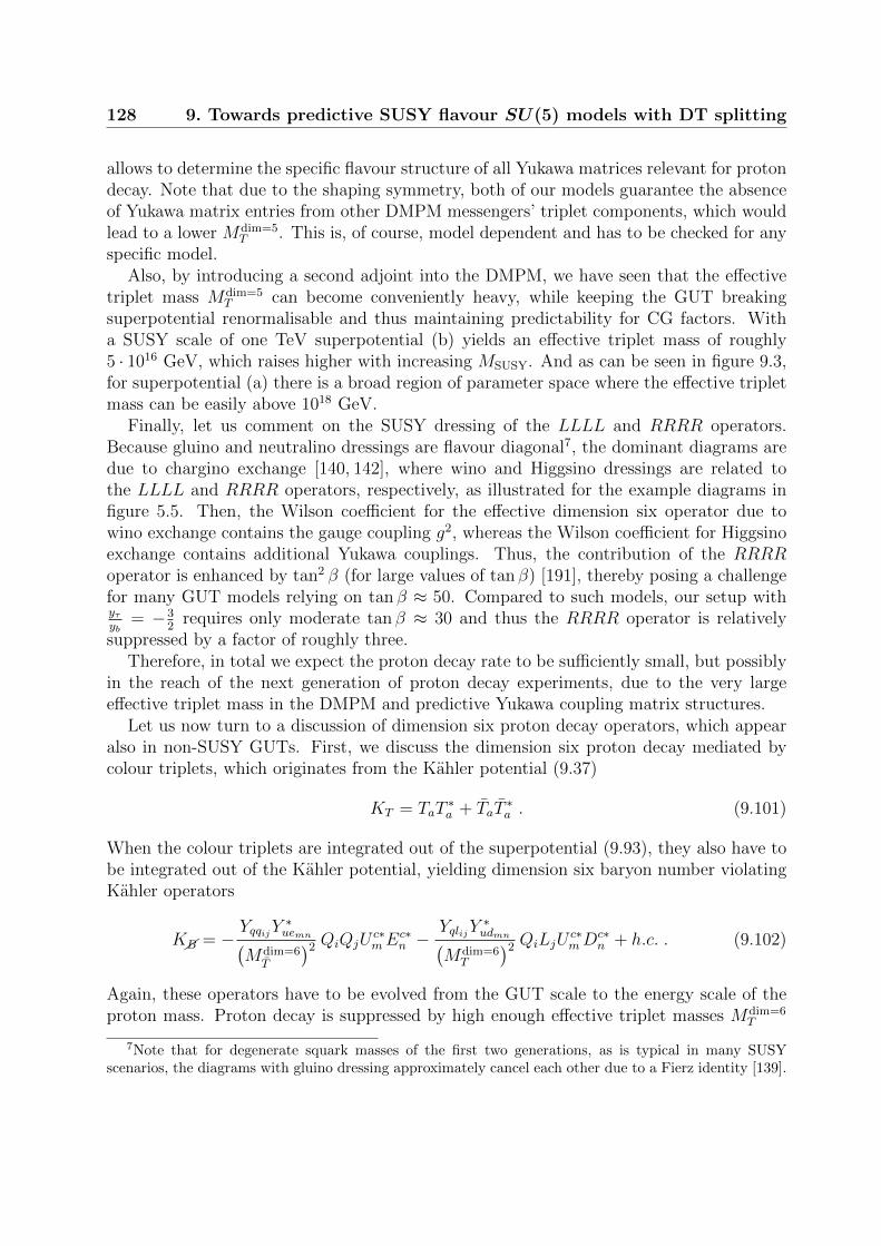
128 9. Towards predictive SUSY flavour SU(5) models with DT splitting
allows to determine the specific flavour structure of all Yukawa matrices relevant for protondecay. Note that due to the shaping symmetry, both of our models guarantee the absenceof Yukawa matrix entries from other DMPM messengers’ triplet components, which wouldlead to a lower Mdim=5
T . This is, of course, model dependent and has to be checked for anyspecific model.
Also, by introducing a second adjoint into the DMPM, we have seen that the effectivetriplet mass Mdim=5
T can become conveniently heavy, while keeping the GUT breakingsuperpotential renormalisable and thus maintaining predictability for CG factors. Witha SUSY scale of one TeV superpotential (b) yields an effective triplet mass of roughly5 · 1016 GeV, which raises higher with increasing MSUSY. And as can be seen in figure 9.3,for superpotential (a) there is a broad region of parameter space where the effective tripletmass can be easily above 1018 GeV.
Finally, let us comment on the SUSY dressing of the LLLL and RRRR operators.Because gluino and neutralino dressings are flavour diagonal7, the dominant diagrams aredue to chargino exchange [140, 142], where wino and Higgsino dressings are related tothe LLLL and RRRR operators, respectively, as illustrated for the example diagrams infigure 5.5. Then, the Wilson coefficient for the effective dimension six operator due towino exchange contains the gauge coupling g2, whereas the Wilson coefficient for Higgsinoexchange contains additional Yukawa couplings. Thus, the contribution of the RRRRoperator is enhanced by tan2 β (for large values of tan β) [191], thereby posing a challengefor many GUT models relying on tan β ≈ 50. Compared to such models, our setup withyτyb
= −32
requires only moderate tan β ≈ 30 and thus the RRRR operator is relativelysuppressed by a factor of roughly three.
Therefore, in total we expect the proton decay rate to be sufficiently small, but possiblyin the reach of the next generation of proton decay experiments, due to the very largeeffective triplet mass in the DMPM and predictive Yukawa coupling matrix structures.
Let us now turn to a discussion of dimension six proton decay operators, which appearalso in non-SUSY GUTs. First, we discuss the dimension six proton decay mediated bycolour triplets, which originates from the Kahler potential (9.37)
KT = TaT∗a + TaT
∗a . (9.101)
When the colour triplets are integrated out of the superpotential (9.93), they also have tobe integrated out of the Kahler potential, yielding dimension six baryon number violatingKahler operators
KB = − YqqijY∗uemn(
Mdim=6T
)2 QiQjUc∗mE
c∗n −
YqlijY∗udmn(
Mdim=6T
)2 QiLjUc∗mD
c∗n + h.c. . (9.102)
Again, these operators have to be evolved from the GUT scale to the energy scale of theproton mass. Proton decay is suppressed by high enough effective triplet masses Mdim=6
T
7Note that for degenerate squark masses of the first two generations, as is typical in many SUSYscenarios, the diagrams with gluino dressing approximately cancel each other due to a Fierz identity [139].
9.5 Proton Decay 129
and Mdim=6T
. Since in terms of superfield components the dimension six operators areeffective four fermion operators, there is no need for a sparticle dressing. Therefore, theresulting proton decay rates are independent of the details of the SUSY spectrum.
We close this chapter by commenting on dimension six proton decay due to heavy Xand Y gauge boson exchange, which due to the higher unification scale in SUSY GUTs areconsidered to be less dangerous [145]. The gauge sector of our SU(5) model is exactly thesame as in minimal SU(5), therefore the proton life time can be estimated by (4.30)
Γp ≈ α2u
m5p
M4GUT
, (9.103)
neglecting effects due to RGE evolution and order one coefficients due to nuclear matrixelements. Since the GUT scale can be easily above 1016 GeV and
√αu ≈ 1
5, the proton
decay rate from dimension six operators is sufficiently small, but possibly in the reach ofthe next generation of proton decay experiments.

130 9. Towards predictive SUSY flavour SU(5) models with DT splitting

PART V
Supersymmetric thresholdcorrections

CHAPTER 10
Predicting the Sparticle Spectrum fromGUTs via SUSY threshold corrections with
SusyTC
In the final chapter of this thesis, we close the last edge of the triangle in figure 1.2 anddiscuss supersymmetric one-loop threshold corrections. In part III of this thesis we dis-cussed how GUTs can feature predictions for quark-lepton Yukawa coupling ratios and forrelations between quark and lepton mixing angles. Whether a flavour GUT model cansuccessfully explain the observations in the flavour sector, depends on the RGE evolutionof the Yukawa matrices from the GUT scale to lower energies. In supersymmetric theories,when the MSSM is matched to the SM, tan β-enhanced supersymmetric threshold correc-tions [131, 132] are essential in the investigation of quark-lepton relations and thus link agiven GUT flavour model to the sparticle spectrum.
Two predictive flavour GUT models were presented in chapters 7 and 8. Here we presentour software tool SusyTC, which was introduced as extension to the Mathematica packageREAP [163] in [5], where we calculated the one-loop SUSY threshold corrections for thefull down-type quark, up-type quark, and charged lepton Yukawa coupling matrices in theelectroweak unbroken phase.
10.1 The REAP extension SusyTC
In our SUSY flavour GUT models in part III, we constructed the GUT scale predictionsye = −1
2yd, yµ = 6ys, and yτ = −3
2yb.
1 Other promising quark-lepton mass ratios at theGUT scale have been discussed in [83, 92, 93], e.g. yµ = 9
2ys, see the discussion in 4.4.
Moreover, many GUT models feature b − τ or b − τ − t unification (for early work seee.g. [138,141,192]), or the Georgi-Jarlskog relations (4.28) [87] as predictions.
1Although Yd and Ye are non-diagonal in (7.10) and (8.11), these GUT scale relations are approxi-mately satisfied after the Yukawa matrices are diagonalised. This can also be seen from a small angleapproximation (6.26).

10.1 The REAP extension SusyTC 133
As mentioned in 5.4 and above, in supersymmetric GUT models the SUSY thresholdcorrections can have an important influence on the Yukawa coupling ratios. When theMSSM is matched to the SM, integrating out the sparticles at loop-level leads to theemergence of effective operators, which can contribute sizeably to the Yukawa couplings,depending on the values of the sparticle masses, tan β, and the soft-breaking trilinearcouplings. Thereby, via the SUSY threshold corrections, a given set of GUT predictionsfor the ratios yτ
yb, yµys
, and yeyd
imposes important constraints on the SUSY spectrum.
With the discovery of the Higgs boson at the LHC [193] and the possible discovery ofsparticles in the near future, the question whether a set of SUSY soft-breaking parameterscan be in agreement with both, specific SUSY threshold corrections as required for realisingthe flavour structure of a GUT model, and constraints from the Higgs boson mass andresults on the sparticle spectrum, gains importance. To accurately study this question, weintroduced the new software tool SusyTC as a major extension to REAP [163].
REAP, which is designed to run Yukawa matrices and neutrino parameters in (SUSY)seesaw scenarios with a proper treatment of the right-handed neutrino thresholds, is aconvenient tool for top-down analyses of flavour (GUT) models, with the advantage of anuser-friendly Wolfram Mathematica front-end. However, the SUSY soft-breaking sector isnot included. In the analysis of our SUSY flavour GUT models in part III, we thereforehad to incorporate the effect of SUSY threshold corrections as mere model parameters atan user-defined “SUSY” scale in a simplified treatment assuming, e.g., degenerate first andsecond generation sparticle masses, without specialising any details on the SUSY sector.Although this procedure is quite SUSY model-independent, it only allows to study theconstraints on the SUSY sector indirectly (i.e. via the introduced additional parametersand with simplifying assumptions), and it is unclear whether an explicit SUSY scenariowith these assumptions and requirements can be realised. Let us remark here that thelatest version of REAP has implemented such a treatment of SUSY threshold corrections asadditional model parameters.
In this chapter however, we want to make full use of the SUSY threshold correctionsto gain information on the SUSY flavour structure from GUTs. We have thus extendedand generalised various formulae in the literature which are needed for a precision analysisof SUSY flavour GUT models and implemented them in our software tool SusyTC. Itincludes the full (i.e. CP violating) MSSM sector, a computation of the sparticle masses,and a careful calculation of the one-loop SUSY threshold corrections for the full Yukawacoupling matrices in the electroweak-unbroken phase. The matching of the MSSM to theSM, including DR to MS conversion, is then automatically performed at the SUSY scale.For a further processing of its results by external software, e.g. for performing a two-loopHiggs mass calculation, SusyTC also calculates the one-loop corrected DR value of µ, theone-loop corrected pole mass of the charged (or the CP-odd) Higgs boson and providesoutput in SLHA conventions as Les Houches file [123,194].
We have developed SusyTC specifically to perform top-down analyses of SUSY flavourGUT models. This is a major difference to other well-known SUSY spectrum generators(e.g. [195–198], see e.g. [199] for a comparison), which run experimental constraints from

134 10. Predicting the Sparticle Spectrum from GUTs with SusyTC
low energies to high energies, apply GUT scale boundary conditions, run back to lowenergies and repeat this procedure iteratively. SusyTC instead starts directly from GUTscale input, which can be defined as general (complex) Yukawa, trilinear, and soft-breakingmass matrices, as well as non-universal gaugino masses and m2
huand m2
hd. The RGEs for
these parameters are solved to obtain their values at low energies, thereby enabling aninvestigation whether the GUT scale Yukawa matrix structures of a given SUSY flavourGUT model are in agreement with experimental data.
10.2 SUSY threshold corrections & numerical
procedure
We now present the numerical procedure and the formulae for the SUSY threshold correc-tions. Note that in this chapter we follow the notation of REAP [163] (see also [105]) and usean RL convention for the Yukawa matrices. These differ from the SLHA conventions [123]used in the previous chapters. They can easily be translated by
REAP & SusyTC Yu Yd Ye Tu Td Te m2u m2
dm2e
SLHA Y Tu Y T
d Y Te T Tu T Td T Te (m2
u)T (m2
d)T (m2
e)T
Thus the MSSM superpotential extended by a type-I seesaw mechanism is given by
WMSSM = YeijEciHd · Lj + YνijN
ciHu · Lj
+ YdijDciHd ·Qj − YuijU c
iHu ·Qj +1
2MnijN
ciN
cj + µHu ·Hd , (10.1)
and the soft-breaking Lagrange density by
−Lsoft =1
2Maλ
aλa + c.c.
+ Teij e∗Rihd · Lj + Tνij ν
∗Rihu · Lj + Tdij d
∗Rihd · Qj − Tuij u∗Rihu · Qj + c.c.
+ Q†im2QijQj + L†im
2LijLj + u∗Rim
2uijuRj + d∗Rim
2dijdRj + e∗Rim
2eijeRj + ν∗Rim
2νijνRj
+m2hu|hu|2 +m2
hd|hd|2 + (m2
3hu · hd + c.c.) . (10.2)
Since REAP includes the RGEs in the type-I seesaw extension of the MSSM (with the DRtwo-loop β-functions for the MSSM Yukawa matrices and the neutrino mass operator givenin [105]), we have calculated the DR two-loop β-functions of the gaugino mass parametersMa, the trilinear couplings Tf , the sfermion squared mass matrices m2
f, and of the soft-
breaking Higgs mass parameters m2hu
and m2hd
in the presence of Yν , Mn, and m2ν , using
the general formulae of [136]. We list these β-functions in appendix E.SusyTC calculates the SUSY scale
Q =√mt1mt2 , (10.3)

10.2 SUSY threshold corrections & numerical procedure 135
where the stop masses are defined by the up-type squark mass eigenstates ui with thelargest mixing to t1 and t2.2 The Yukawa matrices and soft-breaking parameters are thenevolved from the GUT scale to the SUSY scale and REAP automatically integrates out theright-handed neutrinos at their respective mass scales in doing so. Note that we assumethe mass of the right-handed neutrinos to be much larger than the SUSY scale Q. REAP
also features the possibility to add one-loop right-handed neutrino thresholds for the SMparameters, following [200].
At the SUSY scale Q, SusyTC then calculates the tree-level sparticle masses, mixings andthe SUSY threshold corrections. These can be subdivided into two classes: Firstly there aretan β-enhanced threshold corrections, which arise for Yd and Ye since at the one-loop leveldown-type quarks and charged leptons couple to hu via exchange of sparticles, as shownin figure 10.1. These are the most relevant contributions to the corrections of the quark-lepton Yukawa coupling ratios. The corresponding threshold effects to Yu, arising fromeffective couplings to hd, are tan β-suppressed. The second class of threshold correctionsemerges from the supersymmetric loops shown in figure 10.2. While some of them arestrongly suppressed, others are proportional to the soft SUSY-breaking trilinear couplingsand can become important in some cases. A third class of threshold corrections, due towave-function renormalisation of the external fields, will be implemented into a futureversion of SusyTC. Given the precision of our numerical analysis in 10.4, their additionalcontribution can be neglected at present.
Considering heavy sparticles and large Q & TeV, SusyTC calculates the SUSY thresholdcorrections in the electroweak unbroken phase. There are in total twelve types of loopdiagrams, which are shown in figures 10.1 and 10.2 for Yd. In the basis of diagonal squarkmasses the SUSY threshold corrections for Yd are (in terms of DR quantities) given by
Y SMdij
= Y MSSMdij
cos β
(1 +
1
16π2tan β
(ηGij + ηWij + ηBij + ηTij
)+
1
16π2
(εWij + εBij + εTij
))+ TMSSM
dijcos β
1
16π2
(ζGij + ζBij
), (10.4)
where
ηGij = −8
3g2
3
µ∗
M3
H2
(m2di
M23
,m2Qj
M23
),
ηWij =3
2g2
2
M∗2
µH2
(M2
2
µ2,m2Qj
µ2
),
ηBij =3
5g2
1
(1
9
µ∗
M1
H2
(m2di
M21
,m2Qj
M21
)+
1
3
M∗1
µH2
(m2di
µ2,M2
1
µ2
)+
1
6
M∗1
µH2
(M2
1
µ2,m2Qj
µ2
)),
2SusyTC can also be set to use the convention Q =√mu1mu6 or an user-defined fixed value for the
SUSY scale, as described in appendix G.

136 10. Predicting the Sparticle Spectrum from GUTs with SusyTC
ηTij = − 1
µYdij
∑n,m
YdimT†umnYunjH2
(m2un
µ2,m2Qm
µ2
), (10.5)
correspond to the tan β-enhanced loops of Figure 10.1, and
εWij = 12g22C00
(µ2
Q2,M2
2
µ2,m2Qj
µ2
),
εBij =3
5g2
1
(4
3C00
(µ2
Q2,M2
1
µ2,m2di
µ2
)+
2
3C00
(µ2
Q2,M2
1
µ2,m2Qj
µ2
)),
εTij =1
Ydij
∑n,m
YdimY†umnYunjH2
(m2un
µ2,m2Qm
µ2
),
ζGij =8
3g2
3
1
M3
H2
(m2di
M23
,m2Qj
M23
),
ζBij = −3
5g2
1
1
9
1
M1
H2
(m2di
M21
,m2Qj
M21
), (10.6)
correspond to the loops in Figure 10.2, respectively, where the contributions ζGij and ζBij canbecome important in cases of small tan β and large trilinear couplings. The loop functionsH2 and C00 are defined as
H2(x, y) ≡ x log(x)
(1− x)(x− y)+
y log(y)
(1− y)(y − x), (10.7)
C00(q, x, y) ≡1
4
(3
2− log(q) +
x2 log(x)
(1− x)(x− y)+
y2 log(y)
(1− y)(y − x)
). (10.8)
Y , T are the Yukawa and trilinear coupling matrices rotated into the basis where thesquark mass matrices are diagonal, using the transformations
m2Q
= WQm2 diag
QW †Q,
m2u = Wum
2 diagu W †
u ,
Yu = WuYuW†Q,
Tu = WuTuW†Q, (10.9)
and analogously for down-type (s)quarks and charged (s)leptons.The SUSY threshold corrections to Ye are given by
Y SMeij
= Y MSSMeij
cos β
(1 +
1
16π2tan β
(τWij + τBij
)+
1
16π2
(δWij + δBij
))+ TMSSM
eijcos β
1
16π2ξBij , (10.10)

10.2 SUSY threshold corrections & numerical procedure 137
QLid†Rj
h∗u
g
Qid∗Rj
QLid†Rj
h∗u
hu hd
u∗Rn Qm
QLid†RjQi
h∗u
Bhu
hd
QLid†Rj
d∗Rj
h∗u
Bhu
hd
QLid†RjQi
h∗u
Whu
hd
QLid†Rj
h∗u
B
Qid∗Rj
Figure 10.1: tanβ - enhanced SUSY threshold corrections to Yd.
with the tan β-enhanced contributions
τWij =3
2g2
2
M∗2
µH2
(M2
2
µ2,m2Lj
µ2
),
τBij =3
5g2
1
(− µ∗
M1
H2
(m2ei
M21
,m2Lj
M21
)+M∗
1
µH2
(m2ei
µ2,M2
1
µ2
)− 1
2
M∗1
µH2
(M2
1
µ2,m2Lj
µ2
)),
(10.11)
and
δWij = 12g22C00
(µ2
Q2,M2
2
µ2,m2Lj
µ2
),
δBij =3
5g2
1
(−2C00
(µ2
Q2,M2
1
µ2,m2Lj
µ2
)+ 4C00
(µ2
Q2,M2
1
µ2,m2ei
µ2
)),

138 10. Predicting the Sparticle Spectrum from GUTs with SusyTC
QLid†Rj
hd
g
Qid∗Rj
QLid†Rj
hd
hu hd
u∗Rn Qm
QLid†RjQi
hd
B hd
QLid†Rj
d∗Rj
hd
Bhd
QLid†RjQi
hd
W hd
QLid†Rj
hd
B
Qid∗Rj
Figure 10.2: None tanβ - enhanced SUSY threshold corrections to Yd.
ξBij =3
5g2
1
1
M1
H2
(m2ei
M21
,m2Lj
M21
). (10.12)
The diagrams for the Ye SUSY threshold corrections are analogous to the ones in figures10.1 and 10.2, with the exception that the loop diagrams shown in the top rows do notexist.
Turning to Yu, the types of diagrams which were tan β-enhanced for Yd and Ye arenow tan β-suppressed. However, there also exist SUSY threshold corrections which areindependent of tan β and enhanced by large trilinear couplings. These SUSY thresholdcorrections to Yu could have important effects. For example the SUSY threshold correctionsto the top Yukawa coupling yt can be of significance in analyses of the Higgs mass andvacuum stability. The expression for the Yu SUSY threshold corrections can be readilyobtained from the SUSY threshold corrections to Yd (10.4)–(10.6) by the replacement
d→ u ,
cos β → sin β , (10.13)

10.2 SUSY threshold corrections & numerical procedure 139
with the exception of the bino-loops, whose contribution become
ηBij =3
5g2
1
(−2
9
µ∗
M1
H2
(m2di
M21
,m2Qj
M21
)+
2
3
M∗1
µH2
(m2ui
µ2,M2
1
µ2
)− 1
6
M∗1
µH2
(M2
1
µ2,m2Qj
µ2
)),
εBij =3
5g2
1
(8
3C00
(µ2
Q2,M2
1
µ2,m2ui
µ2
)− 2
3C00
(µ2
Q2,M2
1
µ2,m2Qj
µ2
)),
ζBij =3
5g2
1
2
9
1
M1
H2
(m2ui
M21
,m2Qj
M21
), (10.14)
due to the different U(1)Y hypercharges of the (s)particles in the loop. The loop diagramsare identical to the ones of Figure 10.1 and 10.2, with u exchanged by d.
After the SUSY threshold corrections are calculated in the DR scheme, REAP convertsthe Yukawa and gauge couplings to the MS scheme following [194].
Finally SusyTC calculates the values of |µ| and m3 from m2hu
, m2hd
, tan β, and MZ byrequiring the existence of spontaneously broken EW vacuum, analogously to the discussionin 5.4. This is equivalent to vanishing tadpole coefficients, and we employ the one-looptadpole equations of hu and hd to obtain the one-loop corrected DR expressions of (5.69)
µ = eiφµ√
1
2
(tan(2β)
(m2hu
tan β − m2hd
cot β)−M2
Z −Re (ΠTZZ (M2
Z))), (10.15)
with m2hu≡ m2
hu− tu and m2
hd≡ m2
hd− td. In the real (CP conserving) MSSM the
phase φµ is restricted to 0 and π. The expressions for the one-loop tadpoles tu, td, andthe transverse Z-boson self energy ΠT
ZZ are based on [201], but extended to include inter-generational mixing, and presented in appendix F. Because µ enters the one-loop formulaefor the threshold corrections, treating tu, td, and ΠT
ZZ as functions of tree-level parametersis sufficiently accurate. The one-loop expression of the SUSY soft-breaking mass m3 iscalculated as
m3 =
√1
2
(tan(2β)
(m2hu− m2
hd
)− (M2
Z +Re (ΠTZZ (M2
Z))) sin(2β)). (10.16)
If desired, SusyTC allows to outsource a two-loop Higgs mass calculation to externalsoftware, e.g. FeynHiggs [127–129], by calculating the one-loop corrected pole mass mH+
(mA) as input for the complex (real) MSSM
m2H+ =
1
cos(2β)
(m2hu − m2
hd−M2
Z −Re(ΠTZZ
(M2
Z
))+ M2
W
−Re (ΠH+H− (mH+)) + td sin2 β + tu cos2 β
), (10.17)
m2A =
1
cos(2β)
(m2hu − m2
hd−M2
Z −Re(ΠTZZ
(M2
Z
))

140 10. Predicting the Sparticle Spectrum from GUTs with SusyTC
Re (ΠAA (mA)) + td sin2 β + tu cos2 β
), (10.18)
where MW is the DR W-boson mass given as
M2W (Q) = M2
W +Re(ΠTWW
(M2
W
))= g2
v(Q)
2, (10.19)
with MZ and MW pole masses and the DR vacuum expectation value v(Q) given by
v2(Q) = 4M2
Z +Re(ΠTZZ (M2
Z))
35g2
1(Q) + g22(Q)
. (10.20)
As in the previous formulae, the self energies ΠH+H− and ΠAA are based on [201], butare extended to include inter-generational mixing and understood as functions of tree-levelparameters. They are given in appendix F.
10.3 A brief introduction to SusyTC
In this section we provide a “Getting Started” calculation for SusyTC. A full documentationof all features is included in appendix G. Since SusyTC is an extension to REAP, an up-to-date version of REAP-MPT [163] (available at http://reapmpt.hepforge.org) needs to beinstalled on your system. SusyTC consists out of the REAP model file RGEMSSMsoftbroken.m,which is based on the model file RGEMSSM.m of REAP 1.11.2 and additionally contains,among other things, the RGEs of the MSSM soft-breaking parameters and the matchingto the SM, and the file SusyTC.m, which includes the formulae for the sparticle spec-trum and SUSY threshold correction calculations. Both files can be downloaded fromhttp://particlesandcosmology.unibas.ch/pages/SusyTC.htm and have to be copiedinto the local REAP directory.
To begin a calculation with SusyTC, one first needs to import RGEMSSMsoftbroken.m:
Needs["REAP‘RGEMSSMsoftbroken‘"];
The model MSSMsoftbroken is then defined by RGEAdd, including additional options suchas RGEtanβ:
RGEAdd["MSSMsoftbroken",RGEtanβ → 30];
In MSSMsoftbroken all REAP options of the model MSSM are available. The options addition-ally available in SusyTC are given in appendix G. The input is given by RGESetInitial.Let us illustrate some features of SusyTC: To test for example the GUT scale predictionfor the Yukawa coupling ratio yµ
ys= 6, considering a given example parameter point in the
Constrained MSSM, one can type:

10.4 The Sparticle Spectrum predicted from CG factors 141
RGESetInitial[2·10∧16,RGEYd → DiagonalMatrix[1.2·10∧-3, 2.2·10∧-3, 0.16],RGEYe → DiagonalMatrix[1.2·10∧-3, 6·2.2·10∧-3, 0.16],RGEM12 → 2000, RGEA0 → 1000, RGEm0 → 2500];
Of course, any general matrices can be used as input for the Yukawa, trilinear, and soft-breaking matrices, as given by the specific SUSY flavour GUT model under consideration.Also, non-universal gaugino masses, m2
hu, and m2
hdcan be specified. The RGEs are then
solved from the GUT scale to the Z-boson mass scale by
RGESolve[91,2·10∧16];
The ratio of the µ and strange quark Yukawa couplings at the Z-boson mass scale can nowbe obtained with RGEGetSolution, CKMParameters, and MNSParameters:
Yu = RGEGetSolution[91, RGEYu];Yd = RGEGetSolution[91, RGEYd];Ye = RGEGetSolution[91, RGEYe];Mν = RGEGetSolution[91, RGEMν];MNSParameters[Mν,Ye][[3, 2]]/CKMParameters[Yu, Yd][[3, 2]]
Repeating this calculation with all SU(5) CG factors listed in table 2 of [83] and (4.45),one obtains the results shown in figure 10.3.
As described in appendix G, SusyTC can also read and write Les Houches files [123,194]as input and output.
10.4 The Sparticle Spectrum predicted from CG fac-
tors
In this section we apply SusyTC to investigate the constraints on the sparticle spectrumwhich arise from a set of GUT scale predictions for the quark-lepton Yukawa couplingratios when assuming Constrained MSSM boundary conditions for the GUT scale SUSYsoft-breaking parameters.
10.4.1 General discussion
Before performing the numerical analysis for a specific example, let us first outline theconnection between the SUSY spectrum and GUT scale Yukawa coupling predictions in amostly model-independent discussion, with the only assumption of universal SUSY soft-breaking parameters. This assumption might be relaxed in realistic models, however it canbe highly motivated in certain SUSY flavour GUT models. The unification of MSSM super-fields into joint GUT or flavour symmetry representations for example predicts universal

142 10. Predicting the Sparticle Spectrum from GUTs with SusyTC
+ ++ +
+
+
+
+
1-3/2-3 9/2 6 90
1
2
3
4
CG
yμ
ys
Figure 10.3: Example results foryµys
at the electroweak scale, considering the SU(5) CG
factors from (4.45), i.e. the GUT scale predictionsyµys
= CG, for a given example Con-strained MSSM parameter point with tanβ = 30, m1/2 = 2000 GeV, A0 = 1000 GeV, andm0 = 2500 GeV. The area between the dashed gray lines corresponds to the experimentalone sigma range [91].
soft-breaking mass matrices for all superfields in the respective multiplets.3 The absenceof deviation from SM predictions for flavour physics observables is a phenomenologicalhint towards approximately flavour-universal soft-breaking parameters. Finally let us re-mark that specific SUSY breaking mechanisms can indeed predict universal soft-breakingparameters.
Then, the origin for predictions and constraints on the SUSY spectrum arises fromthe fact that to our knowledge there exists no viable combination of GUT scale quark-lepton Yukawa coupling ratios which fit the experimental data without the need for acertain amount of SUSY threshold corrections. In order to obtain the required size ofthese corrections, the ratios of trilinear couplings, gaugino masses, µ, and sfermion massesare constrained by the loop functions of 10.2.4 In particular the SUSY spectrum has to lieclose to a common SUSY scale, in contrast to e.g. Split SUSY scenarios [202], where theseloop functions would get too suppressed. For CMSSM boundary conditions one obtainsconstraints for the ratios between m0, m1/2, and A0. Furthermore, since tan β-enhancedSUSY threshold corrections are most relevant, tan β must not be too small. So far, only
3For example, in SU(5) only two soft-breaking mass matrices, one for F and one for T remain, andin SO(10), where all MSSM superfields are embedded into one 16, there is only one soft-breaking massmatrix.
4Note that this argument is also valid when only one of the first two generation quark-lepton ratios ispredicted together with the third family, since the SUSY threshold corrections in CMSSM-like scenariosare approximately equal for the first two generations.
10.4 The Sparticle Spectrum predicted from CG factors 143
constraints for relative relations between SUSY parameters were discussed. The overallscale is finally constrained by the measured Higgs mass, which is sensitive to the sparticlespectrum due to significant loop corrections.
10.4.2 Numerical analysis with SusyTC
Let us now perform a numerical analysis using our new software SusyTC. We consider GUTscale Yukawa coupling ratios ye
yd= −1
2, yµys
= 6, and yτyb
= −32, which have been used in the
construction of the SUSY flavour SU(5) models of [2–4] presented in the previous chaptersof this thesis, and also e.g. in [203]. A subset of these relation, yµ = 6ys, and yτ = −3
2yb,
has been used in [204]. Note that these relations can either emerge as direct result of CGfactors in SU(5) GUTs or as approximate relation after diagonalisation of the GUT scaleYukawa matrices Yd and Ye. Specifically, our GUT scale Yukawa matrices are given by
Yd =
yd 0 00 ys 00 0 yb
, Ye =
−12yd 0 0
0 6ys 00 0 −3
2yb
,
Yu =
yu 0 00 yc 00 0 yt
UCKM(θ12, θ13, θ23, δ) . (10.21)
As discussed above, we assume CMSSM boundary conditions and restrict our analysisto the parameters m0, m1/2, and A0. The parameter µ is determined from requiring thebreaking of Electroweak symmetry as in (10.15) and we set sgn(µ) = +1. This choice ofreal µ is not in conflict with the framework of the complex MSSM, since in specific modelsof the GUT Higgs potential, as for example the ones discussed in chapter 9, µ can berealised as an effective parameter of the superpotential with a fixed phase, including thecase that µ is real. The last CMSSM parameter tan β is not explicitly included in ouranalysis, however we have scanned over different values of tan β and found that the bestfit can be obtained for values of tan β ≈ 30. For our main analysis we have therefore settan β = 30.
REAP requires a neutrino sector, we have thus added a CSD like (3.43) neutrino Yukawamatrix Yν and right-handed neutrino mass matrix. The entries of Yν have been set tovery small values below O(10−3), such that their effects on the RG evolution can be safelyneglected, and the masses of the right-handed neutrinos to values about 1014 GeV, manyorders of magnitude higher than the expected SUSY scale. Such a neutrino sector is similarto the ones studied in the models of part III and also [203].
Using one-loop RGEs, REAP 1.11.2, and SusyTC we determine the SUSY soft-breakingparameters and µ at the calculated SUSY scale, as well as the pole mass mH+ . Parameterpoints which lead to tachyonic sfermion masses at any rernormalisation scale or which donot allow for Electroweak symmetry breaking are discarded. We then pass our results toFeynHiggs 2.11.2 [127–129] in order to calculate the two-loop corrected Higgs pole massesin the complex MSSM. Finally the MSSM is matched to the SM and we compare our results

144 10. Predicting the Sparticle Spectrum from GUTs with SusyTC
at the electroweak scale with the measured Higgs boson mass of mH = 125.7±0.4 GeV [14]and the quark and charged lepton Yukawa couplings and quark mixing parameters takenfrom [91]. Note that we set the uncertainty of the charged lepton Yukawa couplings to onepercent to account for the estimated theoretical uncertainty, which in our analysis exceedsthe experimental one. Similarly, we estimate a theoretical uncertainty of the Higgs masscalculation of ±3 GeV, as is commonly assumed.5
10.4.3 Results
Of our thirteen parameters, it turned out that by adjusting the seven parameters of Yu,we could always fit the up-type quark Yukawa couplings, the CKM mixing angles, and theCP phase to agree with at least 10−3 relative precision with experimental data.
Thus, the remaining six parameters yd, ys, yb, m0, m1/2, and A0 are used to fit the massof the SM-like Higgs boson and the Yukawa couplings of down-type quarks and chargedleptons. We found a benchmark point with a χ2 = 3.9:
GUT scale input parameters
yd ys yb1.30 · 10−4 2.29 · 10−3 0.162
m0 A0 m1/2
1607.09 −4373.61 786.95
low energy results
ye yµ yτ2.79 · 10−6 5.92 · 10−4 1.00 · 10−2
yd ys yb mh0
1.60 · 10−5 2.82 · 10−4 1.64 · 10−2 125.0 GeV
Let us discuss our results in detail. First note that by looking at the low energy scaleYukawa coupling ratios
yeyd
= 0.17 ,yµys
= 2.10 , andyτyb
= 0.61 , (10.22)
the importance of SUSY threshold corrections in evaluating the GUT scale predictions forYukawa coupling ratios becomes evident. Note that the ratios yield an double ratio (4.43)∣∣∣∣yµys ydye
∣∣∣∣ = 12.4 , (10.23)
5Recently, indications that the theoretical uncertainty in the “large stop mixing” region of parameterspace, which will turn out to be most relevant to our analysis, may be larger, have been discussed [205],however there is no full agreement on this aspect. The improvement of the Higgs mass computation is anactive field of research and future studies will benefit from more precise calculations.

10.4 The Sparticle Spectrum predicted from CG factors 145
within the reported one sigma range. The effect of SUSY threshold corrections can alsoclearly be seen in figure 10.4 as offset at the SUSY scale. Note that the SUSY threshold
yeyd
yμys
yτyb
102 104 106 108 1010 1012 1014 1016
1
0.5
2
6
RG scale (GeV)
Figure 10.4: RG evolution of the Yukawa coupling ratios of the first, second, and thirdfamily from the GUT scale to the electroweak scale. The GUT scale parameters correspondto our benchmark point. The effects of the threshold corrections are clearly visible at theSUSY scale Q = 940 GeV. The light grey areas indicate the experimental Yukawa couplingratios at MZ , taken from [91].
correction necessary to correct the third generation GUT scale prediction yτ = −32
is thesmallest. In fact one can express the ratio of the Yukawa coupling ratios above and belowthe SUSY scale in terms of the parametrisation (7.26), which was employed in chapters 7and 8 to approximate the effect of SUSY threshold corrections without specific knowledgeof the SUSY parameters. We find
1+ diag (ηQ12 , ηQ12 , ηQ3) ≈ diag (1.27, 1.27, 1.17) , (10.24)
i.e. our assumption of equal SUSY threshold corrections for the first and second generationswas justified. This of course is not a surprise, since we assume CMSSM GUT scale boundaryconditions and therefore, as we will see in a moment, the squarks of the first and secondgenerations are approximately degenerate in mass. Such a mass degeneracy was stated in7.4 as condition for (7.26) to be valid.
Because SusyTC calculates the SUSY threshold corrections for the full Yukawa matrices,additionally to the quark-lepton mass ratios, as shown in figure 10.5 one can also determinea considerable effect of the SUSY threshold corrections on the CKM angles, which in general
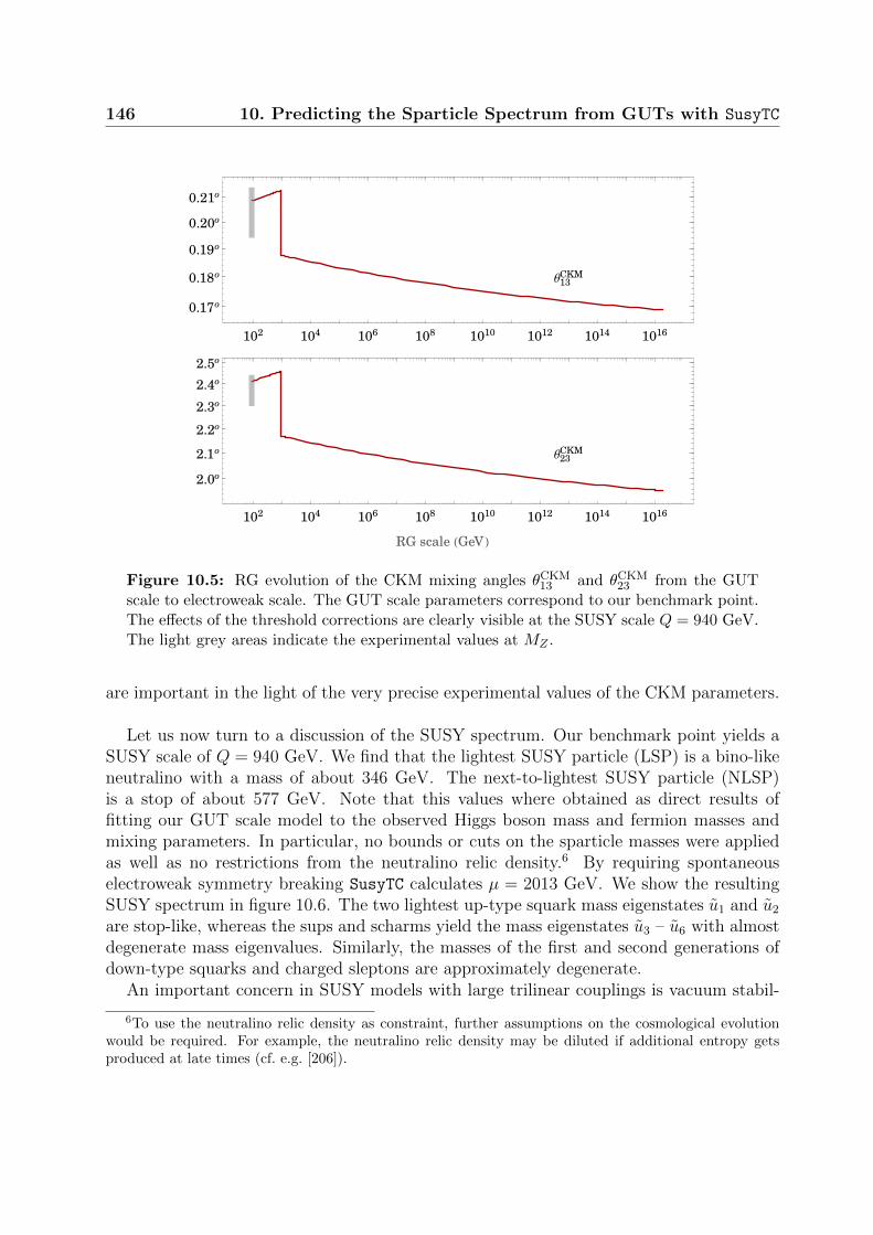
146 10. Predicting the Sparticle Spectrum from GUTs with SusyTC
θ13CKM
102 104 106 108 1010 1012 1014 1016
0.17o
0.18o
0.19o
0.20o
0.21o
θ23CKM
102 104 106 108 1010 1012 1014 1016
2.0o
2.1o
2.2o
2.3o
2.4o2.5o
RG scale (GeV)
Figure 10.5: RG evolution of the CKM mixing angles θCKM13 and θCKM
23 from the GUTscale to electroweak scale. The GUT scale parameters correspond to our benchmark point.The effects of the threshold corrections are clearly visible at the SUSY scale Q = 940 GeV.The light grey areas indicate the experimental values at MZ .
are important in the light of the very precise experimental values of the CKM parameters.
Let us now turn to a discussion of the SUSY spectrum. Our benchmark point yields aSUSY scale of Q = 940 GeV. We find that the lightest SUSY particle (LSP) is a bino-likeneutralino with a mass of about 346 GeV. The next-to-lightest SUSY particle (NLSP)is a stop of about 577 GeV. Note that this values where obtained as direct results offitting our GUT scale model to the observed Higgs boson mass and fermion masses andmixing parameters. In particular, no bounds or cuts on the sparticle masses were appliedas well as no restrictions from the neutralino relic density.6 By requiring spontaneouselectroweak symmetry breaking SusyTC calculates µ = 2013 GeV. We show the resultingSUSY spectrum in figure 10.6. The two lightest up-type squark mass eigenstates u1 and u2
are stop-like, whereas the sups and scharms yield the mass eigenstates u3 – u6 with almostdegenerate mass eigenvalues. Similarly, the masses of the first and second generations ofdown-type squarks and charged sleptons are approximately degenerate.
An important concern in SUSY models with large trilinear couplings is vacuum stabil-
6To use the neutralino relic density as constraint, further assumptions on the cosmological evolutionwould be required. For example, the neutralino relic density may be diluted if additional entropy getsproduced at late times (cf. e.g. [206]).
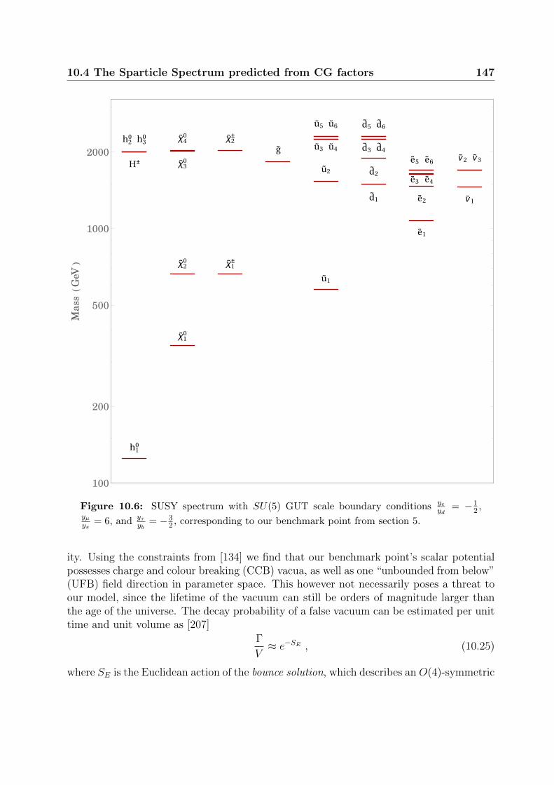
10.4 The Sparticle Spectrum predicted from CG factors 147
h10
h20 h3
0
H±
g
χ10
χ20
χ30
χ40
χ1±
χ2±
u1
u2
u3 u4
u5 u6
d˜
1
d˜
2
d˜
3 d˜
4
d˜
5 d˜
6
e1
e2
e3 e4
e5 e6
ν1
ν2 ν3
100
200
500
1000
2000
Mas
s(G
eV)
Figure 10.6: SUSY spectrum with SU(5) GUT scale boundary conditions yeyd
= −12 ,
yµys
= 6, and yτyb
= −32 , corresponding to our benchmark point from section 5.
ity. Using the constraints from [134] we find that our benchmark point’s scalar potentialpossesses charge and colour breaking (CCB) vacua, as well as one “unbounded from below”(UFB) field direction in parameter space. This however not necessarily poses a threat toour model, since the lifetime of the vacuum can still be orders of magnitude larger thanthe age of the universe. The decay probability of a false vacuum can be estimated per unittime and unit volume as [207]
Γ
V≈ e−SE , (10.25)
where SE is the Euclidean action of the bounce solution, which describes an O(4)-symmetric

148 10. Predicting the Sparticle Spectrum from GUTs with SusyTC
field configuration which, starting at the false vacuum for Euclidean time τ → −∞,“bounces” off the true vacuum at τ = 0, and returns into the false vacuum at τ → ∞.Requiring that the probability of a vacuum decay to happen in our past lightcone is suffi-ciently small translates into a lower bound
SE > 400 . (10.26)
SE can be approximated by considering a straight path ~φ = φ~v connecting false and truevacuum in field space [208].7 We thus study a single scalar field φ with potential U(φ),which has a false vacuum at φ = φf . The bounce solution is then obtained from minimising
SE = 2π2
∫ ∞0
dr r3(z
2∂iφ∂
iφ+ U(φ)), (10.27)
with the boundary conditions φ(τ → ∞) ≡ φf , φ′(0) ≡ 0, and z = 1 if φ is canonically
normalised. The equation of motion is
φ′′(r) +3
rφ′(r) = U ′(φ) , (10.28)
which corresponds to a classical field φ moving in a potential −U(φ) and subject to somefriction force [207]. Following the program of [209], SE can be determined by rephrasingthe directions of “improved CCB” constraints in field space of [134] into the general form
U(φ) = M22φ
2 −M3φ3 + λφ4 . (10.29)
Then SE can be approximated by [210]
SE =z2M2
2
M23
SE(κ) , (10.30)
κ ≡ λM2
2
M23
. (10.31)
Note that SE depends only on a single parameter and can be approximated by the expres-sion [210]
SE(κ) ≈
−0.7 + 2π2
12(1−4κ)3 + 16.5(1−4κ)2 + 28
1−4κκ ≥ 0
45.4(
1 +(
3·45.42π2
)1.1 |κ|1.1)− 1
1.1κ ≤ 0
. (10.32)
Tunneling is possible for any value κ < 14
and values of κ < 0 correspond to “unboundedfrom below” directions. The “improved CCB” directions involve one trilinear term Tf andare in generally D-flat. Only for the case of the top squarks the scalar potential can suffer
7Note that this method yields an upper bound for SE . A complete minimisation of SE over all non-trivial paths is very elaborate and beyond the scope of this thesis. Since our smallest value of SE ≈ 1090satisfies (10.26) by far, the simplified method can be used to estimate a generally small enough decayprobability.
10.4 The Sparticle Spectrum predicted from CG factors 149
from CCB vacua with non-vanishing D-terms. For all trilinear couplings Tuij , Tdij , and Teijwe numerically minimised (10.30) for the corresponding “improved CCB” field directionand checked that SE > 400 is satisfied.
Another strong constraint on the MSSM parameter space comes from the UFB-3 direc-tion [134]
UUFB-3 =
m2hu|hu|2 + |µ|
ydj
(m2Qjj
+ m2djj
)|hu|+ 1
8(g′2 + g2
2)(|hu|2 + |µ|
ydj|hu|)2
|hu| < Hc(m2hu
+ m2Lii
)|hu|2 + |µ|
ydj
(m2Qjj
+ m2djj
+ m2Lii
)|hu| −
2mLiig′2+g2
2|hu| > Hc
,
(10.33)where
Hc ≡√
µ2
4y2dj
+2mLii
g′2 + g22
− |µ|2ydj
, (10.34)
and m2 are the soft-breaking matrices in the Super-CKM/Super-PMNS basis, as definedin appendix B. A second potentially dangerous UFB-3 direction is given by (10.33) withthe replacement Qj, dj → Lj, ej. Both directions depend only on |hu|, thus we use (10.28)to calculate SE. We find that the lifetime of the electroweak vacuum is many orders ofmagnitude larger than the age of the universe, which shows that our model’s benchmarkpoint is phenomenologically viable.
We now discuss confidence intervals for our model’s sparticle masses and parameters,which we obtain as in part III as Bayesian hpd intervals from a Markov Chain Monte Carloanalysis, using a Metropolis algorithm. Looking at fit results for several fixed values of|A0|, we find that in order to avoid potentially dangerous vacuum decay rates, the MCMCanalysis must include a prior for |A0|. A detailed, individual computation of each parameterpoint’s vacuum lifetime, although more desirable than a prior, would consume too muchcomputation time. In our analysis we restrict |A0| < 7.5 TeV, although we remark thatour predicted confidence intervals could be somewhat enlarged by a more sophisticatedinclusion of the lifetime constraints. In figure 10.7 on page 151 we show our results for theone sigma hpd intervals of the sparticle masses. We find that for all parameter points theLSP and NLSP are a bino-like neutralino and a stop, respectively. As a result of the fit andwithout applying any constraints, the masses of all sparticles are above current bounds fromLHC or dark matter searches. The lower band of our predicted sparticle spectrum is withinreach of a future LHC high-luminosity upgrade, and the full range is possibly testable atfuture O(100 TeV) proton-proton colliders like the FCC-hh or the SppC (see e.g. [211]).For the SUSY scale we find an hpd interval of Qhpd = [841, 3092] GeV. Correlation betweenLSP, NLSP, and gluino masses are shown in figure 10.8 as two-dimensional hpd regions.Finally we show the one sigma hpd intervals for the CMSSM soft-breaking parameters infigure 10.9. The correlations between the CMSSM parameters and the resulting mass ofthe SM-like Higgs boson is shown in figure 10.10.

150 10. Predicting the Sparticle Spectrum from GUTs with SusyTC
10.4.4 Remarks
We close this chapter with some remarks and comments on our analysis.
Other GUT scale predictions For our analysis we investigated the GUT scale Yukawacoupling ratios that have been constructed in the various models of this thesis, i.e. yτ
yb= −3
2,
yµys
= 6, and yeyd
= −12. Certainly, other GUT scale relations like Georgi-Jarlskog or the
other CG factors of (4.45) can be constructed, too. We have published SusyTC to providethe SUSY GUT model building community with an useful tool for model analyses and itwill be interesting to compare predictions and constrains on the SUSY spectra from otherpromising GUT scale Yukawa predictions in the future. Also note that some GUT modelsdo not predict any quark-lepton Yukawa coupling ratios, hence they lack a link to theSUSY threshold corrections and do not yield constraints on the SUSY spectrum.
Universal soft-breaking terms As discussed in 10.4.1, universal SUSY soft-breakingparameters are well motivated in SUSY flavour GUT models. However, it will be interest-ing to study constraints on the non-universality of the soft-breaking parameters in futureanalyses. In this context the results obtained with SusyTC can be obtained as SLHA out-put files and the obtained SUSY spectrum can conveniently be forwarded to software toolsspecialised on flavour observables.
Gauge coupling unification A discussion on gauge coupling unification depends stronglyon the GUT Higgs potential and was therefore omitted in this chapter (see e.g. 9.3). Notehowever that GUT threshold effects can be implemented into REAP and one can study theeffects on gauge coupling unification within a complete GUT model. For our analysis, wehave simply fixed the GUT scale at the common 2 · 1016 GeV, which is of similar size ase.g. the GUT scale of the model in 9.4.1. Let us however point at the interesting possi-bility, that the GUT scale is shifted to much higher values. In this case, the RGEs forthe Yukawa couplings have to be solved for a larger range and thus the predictions forthe SUSY spectrum will change. Eventually, a higher GUT scale can possibly even favourother quark-lepton Yukawa coupling ratios than a model with lower GUT scale.

10.4 The Sparticle Spectrum predicted from CG factors 151
h10
h20 h3
0
H±
χ 10
χ 20
χ 30 χ 4
0
χ 1±
χ 2± g
u id i
ei νi
100
200
500
1000
2000
5000
Mas
s(G
eV)
Figure 10.7: One sigma hpd intervals for the sparticle spectrum and Higgs boson masseswith SU(5) GUT scale boundary conditions ye
yd= −1
2 ,yµys
= 6, and yτyb
= −32 , corresponding
to our benchmark point. The LSP is always χ01 and the NLSP is always a stop.

152 10. Predicting the Sparticle Spectrum from GUTs with SusyTC
0 2000 4000 6000 80000
500
1000
1500
2000
mg~ (GeV)
mχ~
10(G
eV)
0 2000 4000 6000 80000
2000
4000
6000
8000
mg~ (GeV)
mu~
1(G
eV)
0 2000 4000 6000 80000
500
1000
1500
2000
mu~ 1 ( GeV)
mχ~
10(G
eV)
Figure 10.8: Two-dimensional one sigma (dark) and two sigma (bright) hpd regions forthe masses of the LSP, NLSP, and gluino. The black star marks the benchmark point.

10.4 The Sparticle Spectrum predicted from CG factors 153
0 2000 4000 6000 8000 10 000 12 000 14 000
m0 (GeV)
1000 2000 3000 4000 5000 6000 7000 8000
m1/2 (GeV)
-7000 -6000 -5000 -4000 -3000 -2000 -1000 0
A 0 (GeV)
Figure 10.9: One sigma hpd intervals for the Constrained MSSM soft-breaking parame-ters.

154 10. Predicting the Sparticle Spectrum from GUTs with SusyTC
0 4000 8000115
120
125
130
135
m0 (GeV)
mh(G
eV)
0 1500 3000 4500115
120
125
130
135
m1/2 (GeV)
mh(G
eV)
0-2000-4000-6000115
120
125
130
135
A 0 (GeV)
mh(G
eV)
Figure 10.10: Two-dimensional one sigma (dark) and two sigma (bright) hpd regions forthe CMSSM soft-breaking parameters and the SM-like Higgs mass. The black star marksthe benchmark point. The dashed lines correspond to the region 125.7± 3 GeV.

PART VI
Summary

CHAPTER 11
Summary and Conclusions
In this thesis we derived and discussed multiple predictions, in particular for the flavourand SUSY flavour structure, arising from a certain class of supersymmetric Grand Uni-fied Theories. Combining SUSY, GUTs, and discrete flavour symmetries into predictiveSUSY flavour GUT models, we investigated the interplay between these three beyond theStandard Model concepts.
When a flavour symmetry gets spontaneously broken, the observed hierarchies andstructures in the flavour sector of a model are explained via flavon fields, which obtainvevs pointing into specific directions in flavour space. Relations between quark and leptonobservables can be explained by GUTs, which can feature predictions for ratios betweenquark and lepton Yukawa couplings. In SUSY flavour GUT models, these predictions areaffected by SUSY threshold corrections, thereby linking a particular flavour GUT model tothe SUSY spectrum. Finally, SUSY GUTs can predict too rapid proton decay, establishingconstraints on the GUT breaking Higgs sector and the model’s symmetries.
We motivated SUSY flavour GUT models, outlined the problems discussed in this thesis,and introduced the necessary theoretical framework in parts I and II.
In part III we focused on the construction of SUSY flavour GUT models. In particular, wediscussed in chapter 6 four simple conditions to construct the interesting phenomenologicalrelation θPMNS
13 ≈ θC sin θPMNS23 in SU(5) GUTs and Pati-Salam models. The basic principle
is the generation of the down-type quark and charged lepton Yukawa matrix elements fromthe same joint GUT operators, which implies that the resulting matrix elements are equalup to group theoretical Clebsch-Gordan factors. This can impose θC ≈ θe12 and thus theCabibbo angle emerges in the charged lepton corrections to θPMNS
13 . In detail, the fourconditions are
Condition 1: The mixing angles θν13 and θe13 should be vanishing.
Condition 2: The Cabibbo angle should be given by θC ≈ θd12, as for example in modelswith θu12 θd12.

157
Condition 3: The GUT scale ratios between the relevant elements of Ye and Yd have tobe predicted, e.g. from CG factors when the entries of Yd and Ye are generated fromsingle joint GUT operators.
Condition 4: The ratio of the two CG factors in θC ≈∣∣∣ c1c2 ∣∣∣ θe12 must be one, i.e. c1 and c2
have to be equal. In SU(5) GUTs an approximate equality between the 1-2 and 2-1elements of Yd has to be required in addition, e.g. by a symmetry in the 1-2 submatrixor via the GST relation and a vanishing 1-1 element.
In a model-independent way, we estimated the possible corrections due to e.g. RGevolution, next-to-leading order terms in the small angle expansion, and the experimentaluncertainty of θPMNS
23 and found it to be less than about O(10%). Within an explicitflavour GUT model, the uncertainty can decrease to about ±0.25, since the estimate canbe replaced by explicit calculations. Specific flavour GUT models can thus possibly bedifferentiated in careful analyses.
Furthermore, we discussed the connection between different neutrino mixing patternsand the Dirac CP phase via the lepton mixing sum rule. With θν13 θC being theonly restriction on the neutrino sector, a future measurement of δPMNS may be viewed as“reconstructing” the value of θν12, provided that a hierarchic charged lepton Yukawa matrixθe13, θ
e23 θC is given.
In chapter 7 we then proposed a first SUSY flavour GUT model, based on SU(5) andan A4 flavour symmetry, where θPMNS
13 ≈ θC sin θPMNS23 is realised, following the conditions
discussed in chapter 6. In order to construct a predictive GUT model, in addition tothe matter and flavon superpotential, we carefully built the full renormalisable messengersector, which guarantees that only specific GUT contractions emerge in the effective super-potentials when the heavy messenger superfields are integrated out. In this way condition3 is ensured: the GUT scale Yukawa matrix elements are generated from single joint opera-tors, yielding predictive quark-lepton relations via group-theoretical CG factors. We madeuse of a novel set of CG-factors, namely c12 = c22 = 6 and c21 = −1
2, which are in excellent
agreement with the current experimental data for msmd
and satisfy condition 4. Our modelis invariant under generalised CP symmetry, which is broken spontaneously by the vevs offlavon fields. In the neutrino sector we constructed tri-bimaximal mixing, which predictsclose-to-maximal CP violation δPMNS ≈ 270 via the lepton mixing sum rule. In the quarksector our model features a right-angled unitarity triangle.
We performed a detailed fit of the model’s 14 parameters to 18 measured observables,taking into account the RG evolution from the GUT scale to lower energies and approximateformulae for SUSY threshold corrections, and found a good best-fit point with a χ2/d.o.f.of 2.0. Bayesian one sigma highest posterior density intervals were obtained from a MarkovChain Monte Carlo analysis. Including the unmeasured neutrino CP phases, our modelmakes six predictions. We discussed our results in the light of newly available data andoutlined how future more precise measurements of the lepton mixing parameters, δCKM,msmd
, and of neutrino-less double beta decay can be used to test our predictions.
158 11. Summary and Conclusions
Part III is completed with chapter 8, where a strong inverse neutrino mass hierarchy wasconstructed in a second SUSY flavour GUT model with SU(5) and A4. The strong inversehierarchy was constructed without fine-tuning, based on an off-diagonal mass matrix ofthe right-handed neutrinos and a novel vacuum alignment for the flavons constituting theneutrino Yukawa matrix, which features θν23 as free parameter and therefore can explainθPMNS
23 6= 45 without the need for charged lepton corrections. Due to the specific phasesof the flavon vevs, our model predicts δPMNS = ϕPMNS = 180.
Constructing the model similar to the one in chapter 7, we again realised the specificrelation θPMNS
13 ≈ θC sin θPMNS23 from charged lepton mixing corrections, linked to quark
mixing by GUT relations. Comparing to chapter 7, we found an even better best-fitwith χ2/d.o.f. = 1.1 in an analogous phenomenological analysis. We discussed the model’spredictions and found a new non-compliance with the most recent global fit value of θPMNS
23 ,which lies in the second octant for inverse neutrino mass ordering, as opposed to the 2013data. However, we also pointed out that precise measurements of θPMNS
23 are still work inprogress and future experiments will be able to settle this question.
We finally pointed out the differences between the predictions of both models of chapters7 and 8 and discussed how they can be discriminated with the data of running and futureexperiments. For the inverse hierarchy model we found the effective mass parameter ofneutrino-less double beta decay to be in reach of the nEXO and AMoRE experiments.A future 50 − 70 km baseline reactor measurement of θPMNS
12 with high precision wouldallow to distinguish both models. Interestingly, although both models differ mainly in theneutrino sector from each other, they feature different predictions of δCKM and could bedistinguished by a precise measurement of the quark mixing CP phase.
Both models of chapters 7 and 8 can be viewed as proof of principle, demonstratingthe successful construction of predictive flavour GUT models with θPMNS
13 ≈ θC sin θPMNS23
and realistic quark-lepton mass ratios. In particular, the sets of shaping symmetries andmessenger superfields presented in appendix D are not expected to be one-of-a-kind im-plementations of our models’ features. We thus understand our constructed realisationsas classes of models, defined by the strategy of predictive GUT scale Yukawa couplingmatrices, built via shaping symmetries, UV-completion due to messenger superfields, andspecific group-theoretical CG factors.
In part IV of this thesis, we discussed how the double missing partner mechanism solutionto the doublet-triplet splitting problem in SUSY SU(5) GUTs can be combined with thestrategy to construct predictive flavour models via specific CG factors for the GUT scalequark-lepton Yukawa coupling ratios.
We have argued that towards this goal a second SU(5) breaking Higgs superfield in theadjoint representation is very useful:
• An additional 24 can be used to split the triplet and octet components of 24 in a renor-malisable superpotential, thereby shifting the upper bound (obtained from the require-ment of gauge coupling unification) of the effective triplet mass mediating dimension

159
five proton decay to higher values, i.e. above the lower bound from non-observation ofproton decay.
• The introduction of a second adjoint is not only an UV-completion, but generally leadsto more freedom for the GUT scale and the effective triplet mass.
• A second adjoint field allows the 24s to be charged under shaping symmetries, which isnecessary for predictive GUT flavour models.
Then the GUT scale and effective triplet masses can be easily made high enough to avoidproblems with proton decay.
We discussed the shaping symmetry and messenger sector of the DMPM with an ad-joint, which guarantee the absence of dangerous Planck scale suppressed operators andgeneralised the notion of effective triplet masses to the case of more than one pair of Higgsfields H, H coupling to matter.
Two explicit flavour models with different predictions for the GUT scale Yukawa matri-ces were constructed, including shaping symmetry and messenger sector, and we presenteda discussion on the careful choice of messenger superfields with respect to phenomenology.We found that both models feature effective triplet masses above current bounds from pro-ton decay. We included all possible effective Planck scale suppressed operators consistentwith our symmetries and found the welcomed emergence of small µ-terms for the lightHiggs doublets, while no dangerous operator existed that could have spoiled our results.Both models stay perturbative until close to the Planck scale.
Finally we discussed proton decay and outlined that flavour GUT models also determinethe Yukawa matrix structures for the Higgs triplet couplings, and thus enable a morepredictive analysis of different proton decay channels than conventional GUT models.
In the final part V, we studied SUSY threshold corrections and discussed their impor-tance for the investigation of GUT scale quark-lepton Yukawa coupling ratios, therebylinking a given flavour GUT model to the SUSY parameters. Thus, via SUSY thresholdcorrections, GUT models can predict properties of the sparticle spectrum from the patternof quark-lepton mass ratios at the GUT scale.
We extended and generalised various formulae in the literature needed for a precisionanalysis of SUSY flavour GUT models, e.g. we calculated the two-loop RGEs of the MSSMsoft-breaking parameters in the seesaw type-I extension and generalised the one-loop cal-culation of µ and of the pole masses mA and mH+ to include inter-generational mixing inthe self energies. We then carefully calculated the one-loop SUSY threshold corrections forthe full down-type quark, up-type quark, and charged lepton Yukawa coupling matrices inthe electroweak unbroken phase.
We implemented these formulae into a new software tool SusyTC, a major extension tothe Mathematica package REAP. SusyTC also calculates the DR sparticle spectrum and theSUSY scale Q, and can provide output in SLHA “Les Houches” files which are the necessaryinput for external software, e.g. for performing a two-loop Higgs mass calculation.

160 11. Summary and Conclusions
With SusyTC we introduced a convenient tool for top-down analyses of SUSY flavourGUT models, accepting general matrices as input for the GUT scale trilinear and soft-breaking mass matrices, analogously to the input of general GUT scale Yukawa matricesin REAP, and non-universal gaugino masses. Together with REAP, the RG evolution to lowenergies is performed, including an automatic calculation of the SUSY scale, automaticmatching of the MSSM to the SM, and DR to MS conversion.
We applied SusyTC to study the predictions of the GUT scale Yukawa coupling rela-tions ye
yd= −1
2, yµys
= 6, and yτyb
= −32, which were used in the construction of the SUSY
flavour GUT models in parts III and IV for the Constrained MSSM parameters and thesparticle masses. We found a benchmark point with χ2 = 3.9 where the LSP is a bino-likeneutralino with a mass of about 346 GeV and the NLSP a stop with a mass of 577 GeV.We performed a Markov Chain Monte Carlo analysis to obtain Bayesian highest posteriordensity intervals for the sparticle masses. Remarkably, without having applied any con-straints from LHC SUSY searches or dark matter searches, we found that the consideredGUT scenario predicts a sparticle spectrum above past LHC sensitivities, but partly withinreach of a future LHC high-luminosity upgrade. O(100) TeV proton-proton colliders likethe FCC-hh or the SppC will be able to test our findings in the future.
In summary, we demonstrated the successful construction of SUSY flavour GUT mod-els with realistic quark-lepton mass ratios and mixing angle relations by presenting andanalysing two explicit models with normal and inverse neutrino mass ordering, respec-tively. In order to predict the flavour structure, we emphasised the importance of a carefulconstruction of additional shaping symmetries and messenger sectors. We then presenteda strategy to combine such predictive SUSY flavour GUT models with the double miss-ing partner mechanism solution to the doublet-triplet splitting problem by introducing asecond GUT breaking Higgs field in the adjoint representation, constructed two examplemodels, and found their proton decay rate sufficiently suppressed due to heavy effectivetriplet masses. Finally we investigated SUSY threshold corrections and found predictionsfor the sparticle spectrum arising from given flavour GUT models, by introducing a newsoftware tool SusyTC, which enables convenient top-down analyses of SUSY flavour GUTmodels. In conclusion, we performed a detailed investigation of predictions for the flavourand SUSY flavour structure arising from different aspects in certain SUSY flavour GUTmodels and provided an useful software tool for analyses of future models.

Appendices

APPENDIX A
Brief review on group theory
In this appendix a brief review on group theory is presented, where we restrict the discussionto the topics relevant in this thesis. In Particle Physics two types of symmetry groups areimportant: Lie groups and small discrete groups. Of special relevance in this thesis are theLie groups SU(N) and the discrete symmetry group A4, which will be discussed in thisappendix based on [80, 212] for SU(N) and [49, 213, 214] for A4. We also briefly reviewgeneralised CP transformations in A4 flavour models, based on [166].
A.1 The special unitary group SU(N)
The special unitary group SU(N) is the group of unitary N×N matrices U with detU = 1.
A N × N unitary matrix has 2N + 2N(N−1)2
= N2 degrees of freedom. If follows fromincluding the additional constraint detU = 1 that SU(N) has dimension N2−1. Thereforeevery element of the group connected to 1N can be written as
U(θ) = eiθaTa
= 1+ iθaTa +O(θ2) , (A.1)
where T a are N2−1 hermitian, traceless1 N×N matrices, called the generators of SU(N).The generators are normalised as
Tr T aT b =1
2δab . (A.2)
They furnish the Lie algebra su(N) and satisfy the commutator relation
[T a, T b] = ifabcTc , (A.3)
where fabc are called structure constants of su(N). It can be shown that they are totallyanti-symmetric.
A representation R of a group is a set of matrices M associated with group elements suchthat the group multiplication is satisfied. More generally, one can find a set of matrices
1Using det eA = eTr A.
A.1 The special unitary group SU(N) 163
T aR specific to the representation R, which satisfy the same commutation rule Eq. (A.3) asthe generators of su(N) and span a basis of the matrices of R. Representations of SU(N)are named after the rank of the representation matrices.
If a representation R has a basis where all T aR can be brought into block-diagonal form,R is called reducible. A reducible representation can be decomposed into the direct sumof irreducible representation. For every irreducible representation r the matrices T ar arenormalised as
Tr T ar Tbr = l(r)δab , (A.4)
where the constants l(r) are named Dynkin index. Another important constant of SU(N)irreducible representations are the quadratic Casimir invariants C2 defined by∑
a
(T ar Tar )ij = C2δij . (A.5)
The simplest irreducible representation is the singlet representation 1 where M(g) = 1
for all elements g and T aR = 0. In order for the Lagrange density to be invariant under anSU(N) symmetry, it has to transform under the singlet representation.
The structure constants themselves span a representation of real (N2 − 1) × (N2 − 1)matrices, known as adjoint representation with
(T aN2−1
)ij
= −ifaij.Of course, the matrices U also form a representation themselves. This irreducible rep-
resentation is called the fundamental representation N and its representation matrices arespanned by T aN = T a. A field transforming under the fundamental representation of SU(N)is an N -dimensional vector
ψi → Uijψj . (A.6)
For every representation R exists a conjugate representation R, whose representationmatrices are given by the complex conjugates M∗. The conjugate representation to thefundamental representation is called anti-fundamental. Its representation matrices arespanned by T a
N= −T a. With the convention ψi ≡ ψ∗i for the position of the indices, a field
transforming in the anti-fundamental representation is an N -dimensional row vector
ψi → ψjUji . (A.7)
Fields transforming under higher dimensional representations are defined as tensors,whose transformation properties are given by the direct product of the transformations ofthe corresponding vectors
ψi1i2...inj1j2...jm→ U i1
i′1U i2
i′2. . . U in
i′nUj1j′1Uj2
j′2 . . . Ujnj′nψ
i′1i′2...i′n
j′1j′2...j
′m. (A.8)
There are two invariant tensors, which can be used to raise and lower indices: The Kro-necker delta δi
j and the totally anti-symmetric Levi-Civita tensor2 εi1i2...iN . Products ofSU(N) tensors are then obtained by the various possibilities to contract SU(N) indices.
2Note that in SU(2) εij can be used to flip the anti-fundamental 2 into the fundamental 2.

164 A. Brief review on group theory
A.2 The discrete group A4
The symmetry group A4 is the group of even permutations of four elements, i.e. the sym-metry group of a solid tetrahedron, and thus has order 4!
2= 12. The twelve elements of A4
are
• The identity ( ).
• Three double transpositions, which are the interchanges of two unrelated pairs (i1, i2)(i3, i4), and have order two.
• Eight 3-cycles (i1, i2, i3) = (i1, i3) (i1, i2) of order three.
Therefore, the generators of A4 are one double transposition S and one 3-cycle T , see tableA.1.
Generator Cycle order n
S (1, 2) (3, 4) 2T (1, 2, 3) = (1, 3) (1, 2) 3
Table A.1: The generators of A4.
A4 has four conjugacy classes NiCni , where Ni is the number of elements in the conju-
gacy class, ni denotes the order of the elements in the conjugacy class, and gi is one elementof the conjugacy class. Besides the trivial 1C1(1), they are 3C2(S) = S, TST 2, T 2ST,4C3(T ) = T, STS, ST, TS, and 4C3(T 2) = T 2, ST 2S, ST 2, T 2S. Since the numberof conjugacy classes equals the number of irreducible representations, there are four irre-ducible representations in A4. Furthermore, it follows from the group theory theorem thatthe order of a finite group equals the sum of the squares of the dimensions of its irreduciblerepresentations, that A4 has three singlets 1, 1′, and 1′′, and one triplet 3. Then thecharacter table of A4 is given by table A.2. From the character table one can find themultiplication rules
r× s =∑t
d(r, s, t)t , (A.9)
1C1(1) 3C2(S) 4C3(T ) 4C3(T 2)
χi(1) 1 1 1 1χi(1
′) 1 1 w w2
χi(1′′) 1 1 w2 w
χi(3) 3 -1 0 0
Table A.2: Character table of A4, where ω ≡ e2πi3 . The character table is unique up to
an exchange of 1′ and 1′′.

A.2 The discrete group A4 165
with
d(r, s, t) =1
12
∑i
ni χi(r)χi(s)χ∗i (t). (A.10)
One obtains for A4
1′ × 1′ = 1′′ ,
1′′ × 1′′ = 1′ ,
1′ × 1′′ = 1 ,
1′ × 3 = 3 ,
1′′ × 3 = 3 ,
3× 3 = 1 + 1′ + 1′′ + 3s + 3a , (A.11)
where 3s and 3a denote a symmetric and antisymmetric product, respectively.In this thesis we use the A4 basis of Ma and Rajasekaran [76], with the generating
elements S and T as shown in table A.3. In this basis, the 1 in 3 × 3 is given by the
S T
1 1 11′ 1 w1′′ 1 w2
3
1 0 00 −1 00 0 −1
0 1 00 0 11 0 0
Table A.3: The generating elements of S and T for the irreducible representations of A4
in the Ma-Rajasekaran basis.
SO(3)-type inner product
3× 3 = 1 :
α1
α2
α3
×β1
β2
β3
= α1β1 + α2β2 + α3β3 . (A.12)
The other singlets in 3× 3 are given by
3× 3 = 1′ :
α1
α2
α3
×β1
β2
β3
= α1β1 + ω2α2β2 + ωα3β3 , (A.13)
3× 3 = 1′′ :
α1
α2
α3
×β1
β2
β3
= α1β1 + ωα2β2 + ω2α3β3 , (A.14)

166 A. Brief review on group theory
where ω ≡ e2πi3 . For the two triplets in 3×3 we denote the symmetric product by “?” and
the antisymmetric by “×”
3 ? 3 = 3s :
α1
α2
α3
?
β1
β2
β3
=1
2
α2β3 + α3β2
α3β1 + α1β3
α1β2 + α2β1
, (A.15)
3× 3 = 3a :
α1
α2
α3
×β1
β2
β3
=1
2
α2β3 − α3β2
α3β1 − α1β3
α1β2 − α2β1
. (A.16)
The remaining products are given by
1′ × 3 = 3 : α×
β1
β2
β3
= α
β1
ωβ2
ω2β2
, (A.17)
1′′ × 3 = 3 : α×
β1
β2
β3
= α
β1
ω2β2
ωβ2
, (A.18)
1′ × 1′′ = 1 : αβ , (A.19)
1′ × 1′ = 1′′ : αβ , (A.20)
1′′ × 1′′ = 1′ : αβ . (A.21)
A.3 Generalised CP transformations
The so called canonical CP violation acts on a scalar field φ as
CP : φ→ eiϕφ∗ . (A.22)
If the field transforms as a (not necessarily irreducible) representation ρ of a flavour sym-metry group G
φ→ ρ(g)φ g ∈ G , (A.23)
a generalised CP transformation [215] is defined by [166]
CP ′ : φ→ Uφ∗ , (A.24)
where U is an unitary matrix acting on flavour space, which has to satisfy a consistencyequation
U−1ρ(g′)U = ρ(g)∗ , (A.25)
since flavour group and generalised CP transformations have to commute.3 Thus, gener-alised CP is an automorphism of the flavour group. If CP ′ is an additional symmetry, U
3Note that the trivial solution U = 1 exists for fields transforming in real representations of G.

A.3 Generalised CP transformations 167
must not be constructed from the generators of G, hence CP ′ is an outer automorphism.Their action on the character table correspond to an exchange of rows and columns.
For the flavour symmetry group A4, the only possibility for a generalised CP transfor-mation is the outer automorphism
u : T → T 2 , (A.26)
since automorphism map elements to elements of the same order. We can check that ualso exchanges the irreducible representations 1′ and 1′′
ρ1′(u(T )) = ρ1′(T2) = Uρ1′(T )∗U−1 = ρ1′(T )∗ = ρ1′′(T ) , (A.27)
since for one-dimensional representations the unitary matrix U can be represented as phase.We can choose U to be real and therefore for the irreducible representations 1, 1′, and 1′′
we find
φ1CP ′−−→ φ∗1 , φ1′
CP ′−−→ φ∗1′ , and φ1′′CP ′−−→ φ∗1′′ . (A.28)
For the triplet representation one can solve for U
ρ3(u(T )) = ρ3(T 2) =
0 0 11 0 00 1 0
= Uρ3(T )∗U−1 = U
0 1 00 0 11 0 0
U−1 (A.29)
and generalised CP is given by
φ3CP ′−−→
1 0 00 0 10 1 0
φ∗3 . (A.30)
Let us briefly illustrate why generalised CP is important by considering a real fieldχ transforming as 3 under A4 and a singlet ζ transforming as 1′′. The canonical CPtransformations would be
CP : χ→ χ , ζ → ζ∗ . (A.31)
Let us investigate the A4 product
(χχ)1′ ζ =(χ2
1 + ω2χ22 + ωχ2
3
)ζ . (A.32)
Under canonical CP this transforms into
(χχ)1′ ζCP ′−−→ (χχ)1′ ζ
∗ , (A.33)
and the transformed product is no longer invariant under A4, since ζ∗ transforms as 1′
and 1′× 1′ = 1′′. Thus canonical CP is not a viable CP transformation, because there arefields transforming in complex representations in the product.

168 A. Brief review on group theory
On the other hand, under generalised CP we have
CP ′ :
χ1
χ2
χ3
→χ1
χ3
χ2
, ζ → ζ∗ . (A.34)
Then (A.32) transforms into
(χχ)1′ ζCP ′−−→
(χ2
1 + ω2χ23 + ωχ2
2
)ζ∗ , (A.35)
which, since (χ21 + ω2χ2
3 + ωχ22) transforms as 1′′, is invariant under A4.
Therefore, in theories with discrete flavour symmetries and fields in complex repre-sentations, the absence of a canonical CP transformation does in general not necessarilycorrespond to CP violation, but rather the physical CP symmetry can correspond to a gen-eralised CP transformation of the flavour group. A categorisation of discrete groups intoexplicitly CP violating groups and groups with generalised CP can be found four examplein [216].
APPENDIX B
Sparticle Mass and Mixing Matrices
Here we show our conventions for the sparticle mass and mixing matrices. We employSLHA 2 conventions [123] in the Super-CKM (SCKM) and Super-PMNS (SPMNS) basis.These bases are obtained from rotating the sfermion fields correspondingly to their fermionpartners, when those are rotated into the mass basis (2.23)
yf ≡ Y diagf =
(U
(f)L
)TYf
(U
(f)R
)∗. (B.1)
Then the soft-breaking matrices in the Super-CKM/Super-PMNS basis are obtained fromour flavour basis (5.65) by
Tf ≡(U
(f)R
)†T Tf
(U
(f)L
),
m2Q≡(U
(d)L
)†m2Q
(U
(d)L
),
m2L≡(U
(e)L
)†m2L
(U
(d)L
),
m2u ≡
(U
(u)R
)† (m2u
)T (U
(u)R
),
m2d≡(U
(d)R
)† (m2d
)T (U
(d)R
),
m2e ≡
(U
(e)R
)† (m2e
)T (U
(e)R
). (B.2)
The sparticle mass matrices are then defined by
L = −Φ†fM2fΦf , (B.3)

170 B. Sparticle Mass and Mixing Matrices
with Φf =(fL1 , fL2 , fL3 , fR1 , fR2 , fR3
)Tand the sparticle mass matrices by
M2u =
(VCKMm
2QV †CKM + v2
2y2u sin2 β +Du,L
v√2T †u sin β − µ v√
2yu cos β
v√2Tu sin β − µ∗ v√
2yu cos β m2
u + v2
2y2u sin2 β +Du,R
),
M2d
=
(m2Q
+ v2
2y2d cos2 β +Dd,L
v√2T †d cos β − µ v√
2yd sin β
v√2Td cos β − µ∗ v√
2yd sin β m2
d+ v2
2y2d cos2 β +Dd,R
),
M2e =
(m2L
+ v2
2y2e cos2 β +De,L
v√2T †e cos β − µ v√
2ye sin β
v√2Te cos β − µ∗ v√
2ye sin β m2
e + v2
2y2e cos2 β +De,R
),
M2ν =V †PMNSm
2LVPMNS +Dν,L . (B.4)
The D-terms are
Df,L = M2Z(I3 −Qe sin2 θW ) cos(2β) 13 ,
Df,R = M2ZQe cos(2β) sin2 θW 13 , (B.5)
where I3 denotes the SU(2)L isospin and Qe the electric charge of the flavour f , and θWdenotes the weak mixing angle. Note that our convention for µ differs by a sign from theconvention in [201].
We define the sfermion mixing matrices by1
M2f
= WfM2 diag
fW †f. (B.6)
The neutralino mixing matrix is defined by
Mψ0 = NTMdiagψ0 N , (B.7)
with
Mψ0 =
M1 0 −MZ cos β sin θW MZ sin β sin θW0 M2 MZ cos β cos θW −MZ sin β cos θW
−MZ cos β sin θW MZ cos β cos θW 0 −µMZ sin β sin θW −MZ sin β cos θW −µ 0
.
(B.8)The chargino mixing matrix is defined by
Mψ+ = UTMdiagψ+ V , (B.9)
with
Mψ+ =
(M2
√2MW sin β√
2MW cos β µ
). (B.10)
1The SLHA 2 convention sfermion mixing matrices Rf can be obtained via Rf = W †f
.

APPENDIX C
Markov Chain Monte Carlo techniques
In this appendix we briefly review Markov Chain Monte Carlo methods, based on [14,217].The Monte Carlo technique uses large numbers of (pseudo) random numbers to calculate
approximations for integrals, e.g. the expectation value of a complicated probability densitydistribution (pdf). A Markov Chain (MC) is a sequence of random variables1 Xt, wherethe prediction for the next random variable Xt+1 depends only on the current variable Xt,and not on any earlier states. Under the conditions that the MC is
irreducible : The MC does not posses independent cycles. In other words, every statecan be reached from every other state (not necessarily in one step, though).
aperiodic : The lengths of all possible cycles starting at any state and returning to ithave greatest common divisor one.
positive recurrent : Any state of the MC is revisited in finite time.
it has a stationary distribution π, where the probability of being in a particular state isindependent of the initial condition. For a large number of time steps the MC approachesπ as limit.
A Markov Chain Monte Carlo method samples a complicated (posterior) pdf p(θ) bygenerating a Markov Chain whose stationary distribution is given by p. A simple MCMCmethod is the Metropolis algorithm [218].
1. Start with any initial point θ0 with p(θ0) > 0.
2. With the current value θ0, draw a new candidate point θ′ from a proposal densityfunction q(θ′|θ0). q can be any symmetric pdf, i.e. q(θ1|θ2) = q(θ2|θ1). We will usean uncorrelated multivariate normal distribution with mean θ0.
3. Form the acceptance probability α = min(
1, p(θ′)
p(θ0)
).
1We restrict the discussion here to one-dimensional random variables. A generalisation to more dimen-sions is straightforward.

172 C. Markov Chain Monte Carlo techniques
4. Generate a random number u uniformly distributed in [0, 1].
5. If u ≤ α, accept the new value and set θ0 = θ′. Otherwise, θ′ is rejected and the oldpoint θ0 stays.
6. Repeat from step 2.
When fitting a model to data points with mean yi and standard deviation σi, the pos-terior pdf we are interested in is the likelihood function
L(θ) = e−χ2(θ)
2 (C.1)
with
χ2(θ) =∑i
(yi(θ)− yi)2
σ2i
. (C.2)
Starting from θ0, the Metropolis algorithm will draw new candidates θ′. While all param-eter points with higher likelihood are accepted, a few parameters with worse χ2 are alsoaccepted and allow the chain to browse a wider region of parameters space and e.g. escapelocal minima. Eventually the MC convergences to its equilibrium, which constitutes thedesired result. The first time steps until equilibrium is reached are denoted as “burn-inphase” and removed from the analysis. The efficiency of the Metropolis algorithm canbe tuned by the step width ∆ of the proposal density function, which in our case are thestandard deviations of the multivariate normal distribution. For too small ∆, the staycount for each step is very small and parameter space is explored very badly. For too large∆, the stay counts are high and the MCMC has to be run longer to build up statistics.Optimal performance is achieved with an acceptance rate racc of about 40%, decreasingtowards 20% for large numbers of parameters. This is illustrated for three choices of ∆in figure C.1. The optimal choice for the proposal pdf is similar to the target pdf and itsstep-width is close to the the targets pdf standard deviation.
Whether the Metropolis algorithm has converged can be inspected by looking at thetrace plots. A numerical criteria for convergence we use in this thesis is the potential scalereduction factor (psrf) R suggested by Gelman and Rubin [219]
1. Instead of a single, very long MCMC, calculate m chains of length n.
2. Calculate the within-chain variance W ≡ 1m
∑mj=1 s
2j , where sj is the variance of the
i = 1 . . . n values θij in the jth chain: s2j = 1
n−1
∑ni=1
(θij − θj
)2and θj is the mean of
all θij.
3. Calculate the between-chain variance B ≡ nm−1
∑mj=1
(θj − ¯θ
)2
, where ¯θ is the mean
of the j = 1 . . .m values of θj.
4. Calculate R =√
n−1n
+ 1nBW
.

173
0 500 1000 1500 200039.8
39.9
40.0
40.1
40.2
40.3
0 500 1000 1500 2000
-20
0
20
40
60
0 500 1000 1500 2000
-20
0
20
40
60
Figure C.1: Trace plots for Metropolis MCMC analyses. For too small ∆ with small staycounts and racc = 1 (left). With too high ∆ and bad mixing with racc = 0.1% (right). Andwith optimal ∆ and good mixing with racc = 40% (center). The burn-in-phase makes upabout 400 steps.
The psrf thus compares within-chain and between-chain variance. For R > 1.1 the MCMCshould be run longer to improve convergence. The MCMC is assumed to have convergedfor R ≈ 1. For higher-dimensional θ the psrf have to be calculated for each parameterindividually.
Let us now briefly discuss Bayesian confidence intervals. We obtain a posterior pdf fromthe MCMC analysis and are interested in the marginalised posterior probability densityfor particular parameters.2 The confidence interval is then given by the region where theposterior pdf is highest. A z sigma highest posterior density (hpd) interval is the interval[θL,θH ], such that∫ θH
θL
p(θ)dθ = erf
(z√2
)and p(θ ∈ hpd) > p(θ 6∈ hpd) . (C.3)
As shown in figure C.2 the definition of the hpd “confidence interval” agrees with theFrequentist’s confidence interval (CI) if the posterior pdf is a normal distribution. Fornon-symmetric posterior pdfs or pdfs with several peaks, the hpd intervals allow for ageneralisation of the common CIs.
In order to investigate correlations between parameters, (C.3) can be generalised for two
2Here we use the word parameter to describe the fit parameters as well as variables of the fit results.

174 C. Markov Chain Monte Carlo techniques
Figure C.2: One sigma hpd intervals for a normal distribution (left) and for an exampleposterior pdf with two peaks.
or more parameters. An example for a two-dimensional hpd region is shown in figure C.3.
Figure C.3: Example for a two-dimensional hpd region for one sigma (gold) and threesigma (grey). The one sigma hpd intervals for the individual parameters are shown asdashed lines. The star marks the mean value of the MCMC analysis.

APPENDIX D
Appendices to the flavour GUT models
In this appendix we give detailed lists of the messenger fields, shaping symmetries, andsupergraphs, which yield the effective superpotentials of the flavour models of parts IIIand IV.
D.1 Appendix to chapter 7
The quantum numbers of the matter, Higgs, flavon, and driving superfields under SU(5),A4, and the shaping symmetry, are presented in table D.1. In table D.2 the quantumnumbers of the messenger fields Φi are explicitly shown. For each field Φi there is acorresponding field Φi with “opposite” quantum numbers, i.e. quantum numbers such thata mass term ΛiΦiΦi is allowed in the superpotential. Since the quantum numbers of Φi
can be trivially reconstructed from the corresponding Φi, we do not show them explicitlyfor the sake of brevity.
As discussed in 7.1, in order not to generate undesired effective operators, the messengersector has to be selected carefully and the choice of the messenger fields is not unique. Inthe following figures D.1–D.6 we present the supergraphs that give rise to the effectivesuperpotential operators of 7.2 and 7.3, when the heavy messenger fields are integratedout. Each supergraph topology in figures D.1–D.5 corresponds to several operators, whichare shown in the table below each graph. In each of the supergraphs, the external fields,which can be either matter, Higgs, flavon, or driving superfields, are labelled by ϕi, whereasthe messenger fields are labelled by γi and γi, respectively. Note that many of the messengerfields occur in more than one operator.
Finally let us comment on the consistency of the different orders of magnitude for thenumerical values of the ε-parameters defined in (7.10) and (7.12) and given in table 7.2.They arise as effective couplings after the heavy messenger fields are intergrated out andthe vevs of the flavon and GUT Higgs superfields are inserted in the corresponding non-renormalisable operators. As can be checked from figures D.1–D.6, the different ordersof magnitude of the parameters, which are needed to fit the data, can originate from anappropriate choice for the masses of the individual messenger fields, which appear in the

176 D. Appendices to the flavour GUT models
SU(5) A4 Z(a)2 Z(b)
2 Z(a)6 Z(b)
6 Z(c)6 Z(d)
6 Z(e)6 U(1)a U(1)b U(1)R
Matter superfields
F 5 3 . . . 4 4 . . . 2 1T1 10 . . . . . . . . . 1 1T2 10 . . . 1 . 4 . . . 1 1T3 10 . 1 . . . 2 . . . 1 1N c
1 . . . . . 2 2 1 . . . 1N c
2 . . . . . 2 2 1 1 . . 1
Higgs superfields
H5 5 . . . . . 2 . . . -2 .H5 5 . . 1 . 2 . . . -1 . .H45 45 . . . . 4 5 . . 1 . 2H45 45 . . . . 2 1 . . -1 . .H24 24 . . . . . . . . 1 -3 .
Flavon superfields
φ2 . 3 . . . . 1 . . . . .φ3 . 3 1 1 . . . . . . . .φab . 3 . 1 5 . 4 . . . . .φN1 . 3 . . . . 4 5 . . . .φN2 . 3 . . . . 4 5 5 . . .χ . 1′ 1 1 . . 5 . . . . .ξ12 . . . . 1 . . . . . . .ξ23 . . 1 . 5 . 4 . . . . .ξM . . . . . 1 . . . . . .
Driving superfields
S . . . . . . . . . . . 2Dαab . . . . 2 . 4 . . . . 2
Dβab . . . 1 3 . . . . . . 2
Dγab . . . . 4 . 2 . . . . 2
DN1 . . . . . . . 3 . . . 2D′N2
. 1′ . . . . 4 2 2 . . 2
D′′N2. 1′′ . . . . 4 2 2 . . 2
A2 . 3 . . . . 4 . . . . 2A3 . 3 . . . . . . . . . 2O2;3 . . 1 1 . . 5 . . . . 2ON1;N2 . . . . . . 4 2 1 . . 2
Table D.1: The matter, Higgs, flavon, and driving superfields of the model in chapter 7.A dot means that the field is an invariant singlet under the respective symmetry. Note thatthe U(1) symmetries will get explicitly broken to Zn symmetries by the Higgs sector.

D.1 Appendix to chapter 7 177
SU(5) A4 Z(a)2 Z(b)
2 Z(a)6 Z(b)
6 Z(c)6 Z(d)
6 Z(e)6 U(1)a U(1)b U(1)R
Φ1 5 . . . . 4 2 5 . . 2 1Φ2 5 . . . . 4 2 5 5 . 2 1Φ3 5 . 1 . 1 . . . . . 2 2Φ4 . 3 . . 2 . 4 . . . . 2Φ5 . 3 . . . . 4 2 . . . 2Φ6 45 . . . . 4 5 . . 1 -1 1Φ7 5 . . . . 2 1 . . . -2 1Φ8 5 3 . . 1 4 2 . . 1 . 2Φ9 10 . . . 5 . 2 . . -1 2 1Φ10 5 . 1 1 . 4 4 . . 1 -1 1Φ11 5 . 1 1 . 2 2 . . . -2 1Φ12 10 3 . 1 . . 4 . . . -1 1Φ13 . 1′ . . 2 . 4 . . . . 2Φ14 . 1′′ . . 2 . 4 . . . . 2Φ15 . . . . 4 . . . . . . 2Φ16 . . . . 3 . . . . . . .Φ17 . . . . . 4 . . . . . 2Φ18 . . . . . 3 . . . . . .Φ19 . 1′ . . . . 2 . . . . 2Φ20 . . 1 1 . . 3 . . . . .Φ21 . 3 1 . 3 . . . . . . .Φ22 . . . . . 4 4 2 2 . . 2Φ23 . . . . . . 4 2 2 . . 2Φ24 . . . . . 4 4 2 . . . 2Φ25 . . . . . . 4 2 . . . 2Φ26 . . . . . . 4 . . . . 2Φ27 . . . . . . 2 . . . . 2Φ28 10 . . . . . 4 . . . 1 .Φ29 . . . . . . 2 4 4 . . 2Φ30 . 3 . . . . 2 4 . . . 2Φ31 . . . . 5 . . . . . . .Φ32 5 3 . 1 . 4 5 . . 1 . 2Φ33 10 1′′ . 1 . . 5 . . -1 2 1Φ34 10 1′′ . 1 . . 5 . . . -1 1
Table D.2: The messenger fields of the SUSY flavour GUT model in chapter 7. To eachΦi there exists an Φi with “opposite” quantum numbers. A dot means that the field is aninvariant singlet under the respective symmetry. Note that the U(1) symmetries will getexplicitly broken to Zn symmetries by the Higgs sector.
corresponding effective operators. For example, consider the parameters ε2, ε3, and εχ. Up

178 D. Appendices to the flavour GUT models
×ϕ1
ϕ2
γ1 γ1
ϕ3
ϕ4
operator ϕ1 ϕ2 ϕ3 ϕ4 γ1
#1 N c1 H5 φN1 F Φ1
#2 N c2 H5 φN2 F Φ2
#3 ξ23 H5 T2 T3 Φ3
#4 φab φab φab Dβab Φ4
#5 φN1 φN1 φN1 DN1 Φ5
Figure D.1: List of order 4 operators in the effective superpotential.
× ×ϕ1
ϕ2
γ1 γ1
ϕ3
γ2 γ2
ϕ4
ϕ5
operator ϕ1 ϕ2 ϕ3 ϕ4 ϕ5 γ1 γ2
#6 T1 H45 H24 φ2 F Φ6 Φ7
#7 φab H5 F T2 H24 Φ8 Φ9
#8 T3 H5 H24 φ3 F Φ10 Φ11
#9 φab T2 H5 φab T2 Φ12 Φ12
#10 φab φab Dγab φab φab Φ13 Φ14
#11 φab φab Dγab φab φab Φ4 Φ4
Figure D.2: List of order 5 operators in the effective superpotential.
to messenger couplings which may be assumed to be O(1), they are given by
ε2 =〈H24〉〈φ2〉
Λ6Λ7
, ε3 =〈H24〉〈φ3〉
Λ10Λ11
, εχ =〈H24〉〈φ2〉〈χ〉
Λ32Λ33Λ34
. (D.1)
These messenger mass scales are specific to these parameters and therefore the hierarchy
|ε2| |εχ| |ε3| (D.2)

D.1 Appendix to chapter 7 179
× × × ×ϕ1
ϕ2 ϕ3 ϕ4 ϕ5 ϕ6
ϕ7γ1 γ1 γ2 γ2 γ3 γ3 γ4 γ4
operator ϕ1 ϕ2 ϕ3 ϕ4 ϕ5 ϕ6 ϕ7 γ1 γ2 γ3 γ4
#12 ξ12 ξ12 ξ12 S ξ12 ξ12 ξ12 Φ15 Φ16 Φ16 Φ15
#13 ξM ξM ξM S ξM ξM ξM Φ17 Φ18 Φ18 Φ17
#14 χ χ χ S χ χ χ Φ19 Φ20 Φ20 Φ19
#15 φab φab ξ23 S ξ23 φab φab Φ4 Φ21 Φ21 Φ4
Figure D.3: List of order 7 operators in the effective superpotential from supergraphswith linear topology.
× ×
×ϕ1
ϕ2
ϕ3 ϕ4
ϕ5
ϕ6γ1 γ1 γ2 γ2
γ3
γ3
operator ϕ1 ϕ2 ϕ3 ϕ4 ϕ5 ϕ6 γ1 γ2 γ3
#16 ξM ξM φN2 φN2 N c2 N c
2 Φ17 Φ22 Φ23
#17 ξM ξM φN1 φN1 N c1 N c
1 Φ17 Φ24 Φ25
Figure D.4: List of order 6 operators in the effective superpotential from supergraphswith non-linear topology.
can arise from a hierarchy of
Λ10Λ11 Λ32Λ33Λ34
〈χ〉 Λ6Λ7 . (D.3)
Similar arguments hold for the other parameters in chapter 7.

180 D. Appendices to the flavour GUT models
× × ×
×ϕ1
ϕ2
ϕ3 ϕ4
ϕ5 ϕ6
ϕ7γ1 γ1 γ2 γ2 γ3 γ3
γ4
γ4
operator ϕ1 ϕ2 ϕ3 ϕ4 ϕ5 ϕ6 ϕ7 γ1 γ2 γ3 γ4
#18 φ2 φ2 φ2 φ2 T1 T1 H5 Φ26 Φ27 Φ28 Φ26
#19 φN2 φN2 φN2 φN2 S φN2 φN2 Φ23 Φ29 Φ23 Φ23
#20 φN1 φN1 φN1 φN1 S φN1 φN1 Φ25 Φ30 Φ5 Φ5
#21 S ξ12 ξ12 ξ12 ξ12 ξ12 ξ12 Φ31 Φ16 Φ15 Φ15
#22 φ2 φ2 φ2 φ2 S φ2 φ2 Φ26 Φ27 Φ26 Φ26
Figure D.5: List of order 7 operators in the effective superpotential from supergraphswith non-linear topology.
× × ×φ2
H5 F H24 T3
χΦ32 Φ32 Φ33 Φ33 Φ34 Φ34
× ×
×
× ×ξ12
ξ12 ξ12
ξ12 ξ12
T2 T1
H5
Φ15 Φ15 Φ16 Φ16 Φ31 Φ31 Φ28 Φ28
Φ15
Φ15
Figure D.6: Additional effective operators of order 6: [T3H24]10 [FH5]10 χφ2 (top) andof order 8: T1T2ξ
512H5 (bottom).
D.2 Appendix to chapter 8
First we show the quantum numbers of the matter, Higgs, flavon, and driving superfields ofour second SUSY flavour GUT model under SU(5), A4, and the shaping symmetry in tableD.3. In table D.4, half of the messenger superfields and their charges under the model’s

D.2 Appendix to chapter 8 181
symmetry are listed. Again, to each messenger superfield Φi a “partner” Φi exists, suchthat they form a mass term ΛiΦiΦi in the renormalisable superpotential. The charges ofΦi are not given in the table, since they can be trivially determined from the charges ofthe corresponding field Φi.
Let us stress again the importance of the messenger sector to obtain a predictive SUSYflavour GUT model. Without a renormalisable superpotential that UV completes the ef-fective superpotentials in chapter 8, the model’s symmetries could e.g. allow for effectiveoperators which yield undesired large Yukawa matrix elements where a vanishing entry isdesired. In addition, due to many possibilities to contract SU(5) indices, linear combi-nations of effective terms with different CG factors would appear and the model wouldlose its ability to predict viable GUT scale quark-lepton mass ratios. We have thereforecarefully constructed the renormalisable messenger superpotential, which gives rise to thesuperpotentials of chapter 8 when the heavy messenger superfields are integrated out. Itis presented in the form of supergraphs shown in the figures D.7–D.12. As in the appendixto chapter 7, for each supergraph topology we list all operators in tables below each graph,denoting external fields as ϕi and messenger fields as γi and γi.
×ϕ1
ϕ2
γ1 γ1
ϕ3
ϕ4
operator ϕ1 ϕ2 ϕ3 ϕ4 γ1
#1 N c1 H5 φ1 F Φ1
#2 N c2 H5 φbc F Φ2
#3 ξ23 H5 T2 T3 Φ3
#4 φab φab φab Dβab Φ4
#5 φbc φbc φbc Dβbc Φ5
Figure D.7: List of order 4 operators in the effective superpotential.
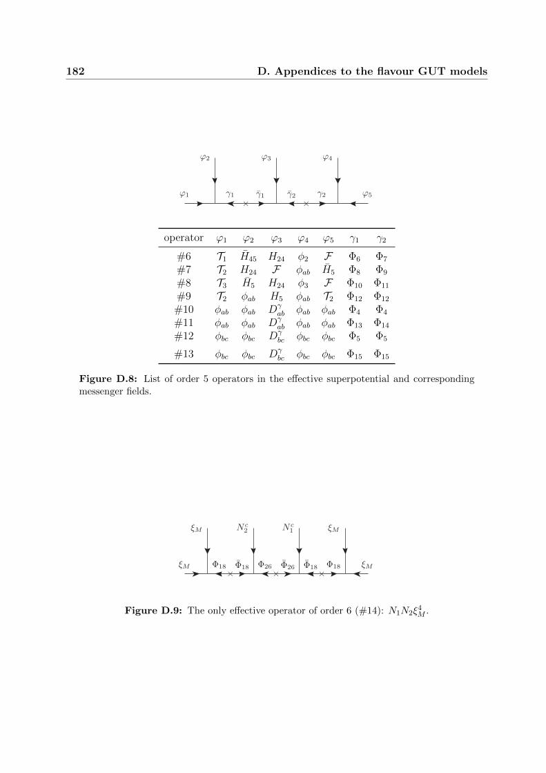
182 D. Appendices to the flavour GUT models
× ×ϕ1
ϕ2
γ1 γ1
ϕ3
γ2 γ2
ϕ4
ϕ5
operator ϕ1 ϕ2 ϕ3 ϕ4 ϕ5 γ1 γ2
#6 T1 H45 H24 φ2 F Φ6 Φ7
#7 T2 H24 F φab H5 Φ8 Φ9
#8 T3 H5 H24 φ3 F Φ10 Φ11
#9 T2 φab H5 φab T2 Φ12 Φ12
#10 φab φab Dγab φab φab Φ4 Φ4
#11 φab φab Dγab φab φab Φ13 Φ14
#12 φbc φbc Dγbc φbc φbc Φ5 Φ5
#13 φbc φbc Dγbc φbc φbc Φ15 Φ15
Figure D.8: List of order 5 operators in the effective superpotential and correspondingmessenger fields.
× × ×ξM
ξM N c2 N c
1 ξM
ξMΦ18 Φ18 Φ26 Φ26 Φ18 Φ18
Figure D.9: The only effective operator of order 6 (#14): N1N2ξ4M .

D.2 Appendix to chapter 8 183
SU(5) A4 Z(a)2 Z(b)
2 Z(a)6 Z(b)
6 Z(c)6 Z(d)
6 U(1)a U(1)b U(1)R
Matter superfields
F 5 3 . . 2 . . 1 2 . 1T1 10 . 1 . . . 1 . 1 . 1T2 10 . . . . 1 . . 1 . 1T3 10 . . 1 . . . . 1 . 1N c
1 . . . . 4 . . 2 . . 1N c
2 . . . . 4 . . 4 . . 1
Higgs superfields
H5 5 . . . . . . . -2 . .H5 5 . . . . . . . . -1 .H45 45 . 1 . . . 2 . . 1 2H45 45 . 1 . . . 4 . . -1 .H24 24 . . . 4 . . 5 -3 1 .
Flavon superfields
φ1 . 3 . . . . . 3 . . .φ2 . 3 . . . . 1 . . . .φ3 . 3 . 1 . . . . . . .φab . 3 . . . 5 . . . . .φbc . 3 . . . . . 1 . . .ξ12 . . 1 . . 1 1 . . . .ξ23 . . . 1 . 5 . . . . .ξM . . . . 1 . . . . . .
Driving superfields
S . . . . . . . . . . 2Dαab . . . . . 2 . . . . 2
Dβab . . . . . 3 . . . . 2
Dγab . . . . . 4 . . . . 2
Dβbc . . . . . . . 3 . . 2
Dγbc . . . . . . . 2 . . 2
O1;2, O′1;2 . 1, 1′ . . . . 5 3 . . 2O1;3, O′1;3 . 1, 1′ . 1 . . . 3 . . 2O2;3, O′2;3 . 1, 1′ . 1 . . 5 . . . 2
Table D.3: The matter, Higgs, flavon, and driving superfields of the SUSY flavour GUTmodel in chapter 8. A dot indicates that the field is an invariant singlet under the cor-responding symmetry. Note that the U(1) symmetries will get explicitly broken to Znsymmetries by the Higgs sector.

184 D. Appendices to the flavour GUT models
SU(5) A4 Z(a)2 Z
(b)2 Z
(a)6 Z
(b)6 Z
(c)6 Z
(d)6 U(1)a U(1)b U(1)R
Φ1 5 . . . 2 . . 4 2 . 1Φ2 5 . . . 2 . . 2 2 . 1Φ3 5 . . 1 . 1 . . 2 . 2Φ4 . 3 . . . 2 . . . . 2Φ5 . 3 . . . . . 4 . . 2Φ6 45 . . . . . 1 . -1 1 1Φ7 5 . . . 4 . 5 5 -2 . 1Φ8 10 . . . 2 5 . 1 2 -1 1Φ9 5 3 . . . 1 . . . 1 2Φ10 5 . . 1 . . . . -1 1 1Φ11 5 . . 1 4 . . 5 -2 . 1Φ12 10 3 . . . . . . -1 . 1Φ13 . 1′ . . . 2 . . . . 2Φ14 . 1′′ . . . 2 . . . . 2Φ15 . . . . . . . 4 . . 2Φ16 . . . . . 4 4 . . . 2Φ17 . . 1 . . 3 3 . . . .Φ18 . . . . 4 . . . . . 2Φ19 . . . . 3 . . . . . .Φ20 . 3 . 1 . 3 . . . . .Φ21 . . . . . . 4 . . . 2Φ22 . . . . . . 2 . . . 2Φ23 10 . 1 . . . 5 . 1 . 1Φ24 . 3 . . . . . 2 . . 2Φ25 . . 1 . . 5 5 . . . .Φ26 . . . . . . . 2 . . 1
Table D.4: The messenger superfields used to generate the effective operators of the modelin chapter 8. To each Φi there exists an Φi with “opposite” quantum numbers. A dot meansthat the field is an invariant singlet under the respective symmetry. Note that the U(1)symmetries will get explicitly broken to Zn symmetries by the Higgs sector.

D.2 Appendix to chapter 8 185
× × × ×ϕ1
ϕ2 ϕ3 ϕ4 ϕ5 ϕ6
ϕ7γ1 γ1 γ2 γ2 γ3 γ3 γ4 γ4
operator ϕ1 ϕ2 ϕ3 ϕ4 ϕ5 ϕ6 ϕ7 γ1 γ2 γ3 γ4
#15 ξ12 ξ12 ξ12 S ξ12 ξ12 ξ12 Φ16 Φ17 Φ17 Φ16
#16 ξM ξM ξM S ξM ξM ξM Φ18 Φ19 Φ19 Φ18
#17 φab φab ξ23 S ξ23 φab φab Φ4 Φ20 Φ20 Φ4
Figure D.10: List of order 7 operators in the effective superpotential from supergraphswith linear topology.
× × ×
×ϕ1
ϕ2
ϕ3 ϕ4
ϕ5 ϕ6
ϕ7γ1 γ1 γ2 γ2 γ3 γ3
γ4
γ4
operator ϕ1 ϕ2 ϕ3 ϕ4 ϕ5 ϕ6 ϕ7 γ1 γ2 γ3 γ4
#18 φ2 φ2 φ2 φ2 T1 T1 H5 Φ21 Φ22 Φ23 Φ21
#19 φbc φbc φbc φbc S φbc φbc Φ15 Φ24 Φ5 Φ5
#20 S ξ12 ξ12 ξ12 ξ12 ξ12 ξ12 Φ25 Φ17 Φ16 Φ16
#21 φ2 φ2 φ2 φ2 S φ2 φ2 Φ21 Φ22 Φ21 Φ21
Figure D.11: List of order 7 operators in the effective superpotential from supergraphswith non-linear topology.

186 D. Appendices to the flavour GUT models
× ×
×
× ×ϕ1
ϕ2 ϕ3
ϕ4 ϕ5
ϕ6 ϕ7
ϕ8
γ1 γ1 γ2 γ2 γ3 γ3 γ4 γ4
γ5
γ5
operator ϕ1 ϕ2 ϕ3 ϕ4 ϕ5 ϕ6 ϕ7 ϕ8 γ1 γ2 γ3 γ4 γ5
#22 ξ12 ξ12 ξ12 ξ12 ξ12 T2 T1 H5 Φ16 Φ17 Φ25 Φ23 Φ16
#23 ξM ξM N c1 φbc φbc N c
1 ξM ξM Φ18 Φ26 Φ26 Φ18 Φ15
Figure D.12: List of order 8 operators in the effective superpotential from supergraphswith non-linear topology.

D.3 Appendix to the first model of chapter 9 187
D.3 Appendix to the first model of chapter 9
In figures D.13 and D.14 we show the supergraphs yielding the effective superpotentialsWd and Wu when the heavy messengers are integrated out.
H ′24
T3
H5
Z5,1Z5,1
F3
〈S′〉
H ′24H5
F2
Z10,1Z10,1
T2
Z10,2 Z10,2
θ3
〈S′〉〈S′〉
H ′24
H24
H5
Z45,1Z45,1
F1
Z45,2 Z45,2
θ4
X45X45
T1
〈S〉〈S′〉 〈S′〉
Figure D.13: Supergraphs leading to the effective superpotentialWd of our model in 9.4.1when the heavy messenger fields get integrated out.
All superfields of the model 9.4.1 are presented in the tables D.5 and D.6, includingtheir charges under the discrete shaping symmetry. As shown in figures D.13 and D.14 themessenger pairs Z5,1Z5,1, Z10,1Z10,1, Z10,2Z10,2, Z45,1Z45,1, and Z45,2Z45,2 get their massesthrough the vevs of S and S ′. The other messengers in the lower part of table D.6 havedirect mass terms, so we do not show the charges of their corresponding conjugated partnersZi, which can be trivially obtained from the charges of Zi.
Let us now discuss the messenger fields appearing in figure D.14 closer. There are threesupergraphs generating the superpotential term y12. The renormalisable superpotentialcorresponding to figure D.14 is
W ⊃ γ1H5T1Z10,4 + γ2H5T2Z10,3 + γ3 T3θ1Z10,3 + γθ θ21Z1
+ λ1 θ2Z2Z1 + λ10 θ2Z10,3Z10,4
+ η1 T1Z10,3Z2 + η2 T2Z10,4Z2 + η′2 T2Z10,3Z1
+ M1 Z1Z1 +M2 Z2Z2 +M10,3 Z10,3Z10,3 +M10,4 Z10,4Z10,4 , (D.4)
where we explicitly denote the coupling constants at the ends of a diagram with γx, couplingconstants in the middle of the diagrams with λx if they involve θj, ηi if they involve Ti,and messenger masses with Mx.
After Zx and Zx are integrated out and the flavons θi obtain vevs, the elements (9.62)

188 D. Appendices to the flavour GUT models
H5 T3
θ1
Z10,3Z10,3
T2
H5 T3
θ1
Z10,4Z10,4
T1
Z10,3 Z10,3
θ2
H5 θ1
θ1
Z10,3Z10,3
T2
Z1 Z1
T2
H5
θ1
θ1
Z10,4Z10,4
T1
Z10,3 Z10,3
θ2
Z1Z1
T2
H5
θ1
θ1
Z10,3Z10,3
T2
Z2 Z2
T1
Z1Z1
θ2
H5
θ1
θ1
Z10,4Z10,4
T1
Z2 Z2
θ2
Z1Z1
T2
H5
θ1
θ1
Z10,4Z10,4
T1
Z10,3 Z10,3
θ2
Z2Z2
T1 θ2
Z1 Z1
Figure D.14: Supergraphs leading to the effective superpotentialWu of our model in 9.4.1when the heavy messenger fields get integrated out. Note that there are three supergraphscontributing to the superpotential term generating y12.
of Yu are given by
y11 = γ1 λ10 η1 λ1 γθ〈θ1〉2〈θ2〉2
M1M2M10,3M10,4
,
y12 = γ2 η1 λ1 γθ〈θ1〉2〈θ2〉
M1M2M10,3
+ γ1 η2 λ1 γθ〈θ1〉2〈θ2〉
M1M2M10,4
+ γ1 λ10 η′2 γθ
〈θ1〉2〈θ2〉M1M10,3M10,4
,

D.3 Appendix to the first model of chapter 9 189
y22 = γ2 η′2 γθ
〈θ1〉2M1M10,3
,
y13 = γ1 λ10 γ3〈θ1〉〈θ2〉M10,3M10,4
,
y23 = γ2 γ3〈θ1〉M10,3
, (D.5)
and y33 is a renormalisable Yukawa coupling coefficient.One might feel motivated to remove the messenger pair Z2, Z2 from the spectrum,
thereby eliminating two supergraphs and thus the first two terms contributing to y12.1 Inthis case however, without Z2Z2, evaluating y12 would yield
y12 = γ1 λ10 η′2 γθ
〈θ1〉2〈θ2〉M1M10,3M10,4
= y13〈θ1〉M1
η′2 γθγ3
= y13 y22M10,3
〈θ1〉1
γ2γ3
=y13y22
y23
. (D.6)
From a small angle expansion of Yu one finds for the mixing angles
θu12 =y12
y22
, θu13 =y13
y33
, and θu23 =y23
y33
, (D.7)
which are identical to the GUT scale CKM mixing angles since our model features diagonalYd. Therefore (D.6) would imply the phenomenologically bad GUT scale relation
θC =θCKM
13
θCKM23
. (D.8)
To fit Yu to the observed data an additional degree of freedom is needed. In our modelthis is realised through Z2Z2 enabling additional diagrams contributing to y12.
This illustrates that besides guaranteeing a certain Yukawa matrix structure and uniqueCG factors, the messenger sector also has to be carefully chosen with respect to its cou-plings, to avoid non-phenomenological predictions for observables.
1A different pair of fields Z ′2, Z ′2 would need to be introduced anyway (using different charge assignmentthan Z2,Z2) in order to generate y11. The charges can be assigned such that no extra contributions to y12
appear.

190 D. Appendices to the flavour GUT models
SU(5) Z2 Z4 Z4 Z4 Z7 Z7 Z9 Z2
Matter and light Higgs superfields
H5 5 . . . . . . . .H5 5 . 2 . . . 1 2 .T1 10 . . 3 . 6 . . 1T2 10 . . . . 6 . . 1T3 10 . . . . . . . 1F1 5 1 1 1 2 1 1 2 1F2 5 1 . . 2 1 . 2 1F3 5 1 2 . 1 . 6 7 1
Superfields with vevs around the GUT scale
H24 24 . . . . . . . .H ′24 24 1 . . . . . . .S 1 . 3 . . . 2 . .S ′ 1 . . . 1 . . . .θ1 1 . . . . 1 . . .θ2 1 . . 1 . . . . .θ3 1 . 2 . . . 6 5 .θ4 1 . . . . . . 5 .
DMPM superfields
H ′5 5 . 3 . . . 5 7 .H ′5 5 . 1 . . . 6 . .X45 45 . 2 . . . 6 7 .X45 45 . 3 . . . 6 2 .Y45 45 . . . . . 3 7 .Y45 45 . 1 . . . 2 2 .Z50 50 . 1 . . . 1 7 .Z50 50 . . . . . 4 2 .X ′45 45 . 3 . . . 1 . .X ′45 45 . 2 . . . 4 . .Y ′45 45 . 1 . . . 5 . .Y ′45 45 . . . . . . . .Z ′50 50 . 2 . . . 3 . .Z ′50 50 . 3 . . . 2 . .
Table D.5: SU(5) representations and charges under the discrete shaping symmetry forthe model of 9.4.1. A dot denotes charge zero.

D.3 Appendix to the first model of chapter 9 191
SU(5) Z2 Z4 Z4 Z4 Z7 Z7 Z9 Z2
Z5,1 5 . 2 . 3 . 1 2 1Z5,1 5 . 2 . . . 6 7 1Z10,1 10 1 . . 3 6 . . 1Z10,1 10 1 . . . 1 . . 1Z10,2 10 1 2 . 2 6 6 5 1Z10,2 10 1 2 . 1 1 1 4 1Z45,1 45 . 3 3 2 6 6 7 1Z45,1 45 . 1 1 1 1 1 2 1Z45,2 45 . 3 3 3 6 6 2 1Z45,2 45 . 1 1 . 1 1 7 1
Z10,3 10 . . . . 1 . . 1Z10,4 10 . . 1 . 1 . . 1Z1 1 . . . . 5 . . .Z2 1 . . 3 . 5 . . .
Table D.6: SU(5) representations and charges under the discrete shaping symmetry ofthe flavon and flavour messenger fields of the model in 9.4.1. Note that the messenger pairsZ5,1Z5,1, Z10,1Z10,1, Z10,2Z10,2, Z45,1Z45,1, and Z45,2Z45,2 have no direct mass term, but gettheir masses through the vevs of S and S′. The other messengers in the lower part of thetable have direct mass terms, so we omit their corresponding conjugated partner Zi. A dotdenotes charge zero.

192 D. Appendices to the flavour GUT models
D.4 Appendix to the second model of chapter 9
Let us first show the supergraphs which generate the effective superpotentials (9.82) and(9.83) in figures D.15 and D.16.
H ′24
T3
H5
Z5,1Z5,1
F3
〈S′〉
F1 H24
T2
Z10,1 Z10,1
H5
Z10,2Z10,2
θ3
〈S′〉〈S′〉
H ′24
H5
F2
Z10,3Z10,3
T2
Z10,4 Z10,4
θ4
〈S′〉〈S′〉
H24
H24
H5
Z45,1Z45,1
F2
X45X45
T1
〈S〉〈S〉
Figure D.15: Supergraphs leading to the effective superpotential Wd when the heavymessenger fields get integrated out in the model 9.4.2.
H5 T3
θ1
Z10,5Z10,5
T2
H5 θ1
θ1
Z10,5Z10,5
T2
Z1 Z1
T2
H5 θ2
θ2
Z10,5Z10,5
T2
Z2 Z2
T1H5 θ2
θ2
Z10,6Z10,6
T1
Z2 Z2
T2
H5 θ5
θ5
Z10,6Z10,6
T1
Z3 Z3
T1
Figure D.16: Supergraphs leading to the effective superpotential Wu when the heavymessenger fields get integrated out in the model 9.4.2.

D.4 Appendix to the second model of chapter 9 193
All superfields of the model and their charges under the model’s symmetries are shownin tables D.7 and D.8. As for the model 9.4.1, some messengers get their masses throughvevs of S and S ′ instead of direct mass terms, as can be seen in figures D.15 and D.16. Themessenger fields in the lower part of table D.7 have direct mass terms, so their correspondingconjugated fields are not shown in the table.
SU(5) Z2 Z3 Z4 Z5 Z6 Z7 Z7 Z2
Z5 5 . 2 1 1 4 6 6 1Z5 5 . 1 . 4 2 1 1 1Z10,1 10 . 1 . 1 . 3 2 1Z10,1 10 . 2 1 4 . 4 5 1Z10,2 10 . . 1 . 4 1 . 1Z10,2 10 . . . . 2 6 . 1Z10,3 10 . 2 . 1 2 6 5 1Z10,3 10 . 1 1 4 4 1 2 1Z10,4 10 . . 1 . 2 1 . 1Z10,4 10 . . . . 4 6 . 1Z45,1 45 . 1 . 2 2 5 4 1Z45,1 45 1 . . 1 4 2 3 1
Z10,5 10 . . . . . 6 . 1Z10,6 10 . . . . . 1 2 1Z1 1 . . . . . 2 . .Z2 1 . . . . . . 5 .Z3 1 . . . . . 5 3 .
Table D.7: SU(5) representations and charges under the discrete shaping symmety of theflavon and flavour messenger fields of the model 9.4.2. Note that the messengers Z5,1Z5,1,Z10,1Z10,1, Z10,2Z10,2, Z10,3Z10,3, Z10,4Z10,4, and Z45,1Z45,1 have no direct mass term, butget their masses through vevs of S and S′, as shown in figures D.15 and D.16. The othermessenger fields in the lower part of the table have direct mass terms, so their correspondingbarred fields are not shown in the table. A dot denotes charge zero.

194 D. Appendices to the flavour GUT models
SU(5) Z2 Z3 Z4 Z5 Z6 Z7 Z7 Z2
Matter and light Higgs superfields
H5 5 . . . . . . . .H5 5 . 2 . 1 4 6 6 .T1 10 . . . . . 6 5 1T2 10 . . . . . 1 . 1T3 10 . . . . . . . 1F1 5 . . . 3 2 5 6 1F2 5 . 2 . 3 . 2 3 1F3 5 . 1 3 4 . 1 1 1
Superfields with vevs around the GUT scale
H24 24 . . . . 4 . . .H ′24 24 . . . . 2 . . .S 1 1 2 . 2 . . . .S ′ 1 . . 3 . . . . .θ1 1 . . . . . 6 . .θ2 1 . . . . . . 1 .θ3 1 . 1 2 1 2 2 2 .θ4 1 . 2 2 1 . 5 5 .θ5 1 . . . . 3 1 2 .
DMPM Superfields
H ′5 5 1 1 . . 4 1 1 .H ′5 5 1 . . 1 2 . . .X45 45 . 1 . 4 4 1 1 .X45 45 1 . . 4 2 6 6 .Y45 45 . 2 . 3 2 1 1 .Y45 45 1 2 . . 4 6 6 .Z50 50 1 . . 1 . 1 1 .Z50 50 . 1 . 2 . 6 6 .X ′45 45 1 . . 4 . . . .X ′45 45 . 1 . 4 . . . .Y ′45 45 1 1 . 3 4 . . .Y ′45 45 . . . . 2 . . .Z ′50 50 . 2 . 1 2 . . .Z ′50 50 1 2 . 2 4 . . .
Table D.8: SU(5) representations and charges under discrete shaping symmetries for themodel of 9.4.2. A dot denotes charge zero.

APPENDIX E
The β-functions in the seesaw type-Iextension of the MSSM
In this appendix we list the β-functions of the SUSY soft-breaking parameters in the MSSMextended by the additional terms in the seesaw type-I extension (obtained using the generalformulae of [136]), which are implemented into REAP and SusyTC. Thus they are given herein our conventions (10.1) and (10.2) for W and Lsoft, respectively.
E.1 One-Loop β-functions
16π2βM1 =66
5g2
1M1 , (E.1)
16π2βM2 = 2g22M2 , (E.2)
16π2βM3 = −6g23M3 , (E.3)
16π2βTu = Yu
(2Y †d Td + 4Y †uTu
)+ Tu
(Y †d Yd + 5Y †uYu
)+ Yu
(6Tr(Y †uTu) + 2Tr(Y †ν Tν) +
26
15g2
1M1 + 6g22M2 +
32
3g2
3M3
)+ Tu
(3Tr(Y †uYu) + Tr(Y †ν Yν)−
13
15g2
1 − 3g22 −
16
3g2
3
), (E.4)
16π2βTd = Yd
(4Y †d Td + 2Y †uTu
)+ Td
(5Y †d Yd + Y †uYu
)+ Yd
(6Tr(Y †d Td) + 2Tr(Y †e Te) +
14
15g2
1M1 + 6g22M2 +
32
3g2
3M3
)+ Td
(3Tr(Y †d Yd) + Tr(Y †e Ye)−
7
15g2
1 − 3g22 −
16
3g2
3
), (E.5)

196 E. The β-functions in the seesaw type-I extension of the MSSM
16π2βTe = Ye(4Y †e Te + 2Y †ν Tν
)+ Te
(5Y †e Ye + Y †ν Yν
)+ Ye
(6Tr(Y †d Td) + 2Tr(Y †e Te) +
18
5g2
1M1 + 6g22M2
)+ Te
(3Tr(Y †d Yd) + Tr(Y †e Ye)−
9
5g2
1 − 3g22
), (E.6)
16π2βTν = Yν(4Y †ν Tν + 2Y †e Te
)+ Tν
(5Y †ν Yν + Y †e Ye
)+ Yν
(6Tr(Y †uTu) + 2Tr(Y †ν Tν) +
6
5g2
1M1 + 6g22M2
)+ Tν
(3Tr(Y †uYu) + Tr(Y †ν Yν)−
3
5g2
1 − 3g22
), (E.7)
16π2βm2L
= 2Y †em2eYe + 2Y †νm
2νYν
+m2L
(Y †e Ye + Y †ν Yν
)+(Y †e Ye + Y †ν Yν
)m2L
+ 2m2huY
†ν Yν + 2m2
hdY †e Ye + 2T †eTe + 2T †νTν
− 6
5g2
1|M1|2 13 − 6g22|M2|2 13 −
3
5g2
1S 13 , (E.8)
16π2βm2Q
= 2Y †um2uYu + 2Y †dm
2dYd
+m2Q
(Y †uYu + Y †d Yd
)+(Y †uYu + Y †d Yd
)m2Q
+ 2m2huY
†uYu + 2m2
hdY †d Yd + 2T †uTu + 2T †dTd
− 2
15g2
1|M1|2 13 − 6g22|M2|2 13 −
32
3g2
3|M3|2 13 +1
5g2
1S 13 , (E.9)
16π2βm2u
= 4Yum2QY †u + 2YuY
†um
2u + 2m2
uYuY†u
+ 4m2huYuY
†u + 4TuT
†u
− 32
15g2
1|M1|2 13 −32
3g2
3|M3|2 13 −4
5g2
1S 13 , (E.10)
16π2βm2d
= 4Ydm2QY †d + 2YdY
†dm
2d
+ 2m2dYdY
†d
+ 4m2hdYdY
†d + 4TdT
†d
− 8
15g2
1|M1|2 13 −32
3g2
3|M3|2 13 +2
5g2
1S 13 , (E.11)

E.2 Two-Loop β-functions 197
16π2βm2e
= 4Yem2LY †e + 2YeY
†em
2e + 2m2
eYeY†e
+ 4m2hdYeY
†e + 4TeT
†e
− 24
5g2
1|M1|2 13 +6
5g2
1S 13 , (E.12)
16π2βm2ν
= 4Yνm2LY †ν + 2YνY
†νm
2ν + 2m2
νYνY†ν
+ 4m2huYνY
†ν + 4TνT
†ν , (E.13)
16π2βm2hd
= 6Tr(Ydm2QY †d + Y †dm
2dY d)
+ 2Tr(Yem2LY †e + Y †em
2eYe)
+ 6m2hd
Tr(Y †d Yd) + 2m2hd
Tr(Y †e Ye)
+ 6Tr(T †dTd) + 2Tr(T †eTe)
− 6
5g2
1|M1|2 − 6g22|M2|2 −
3
5g2
1S , (E.14)
16π2βm2hu
= 6Tr(Yum2QY †u + Y †um
2uY u)
+ 2Tr(Yνm2LY †ν + Y †νm
2νYν)
+ 6m2huTr(Y †uYu) + 2m2
huTr(Y †ν Yν)
+ 6Tr(T †uTu) + 2Tr(T †νTν)
− 6
5g2
1|M1|2 − 6g22|M2|2 +
3
5g2
1S , (E.15)
withS = m2
hu −m2hd
+ Tr(m2Q−m2
L+m2
d+m2
e − 2m2u
). (E.16)
E.2 Two-Loop β-functions
(16π2)2β(2)M1
=12
5g2
1Tr(TνY†ν ) +
28
5g2
1Tr(TdY†d ) +
36
5g2
1Tr(TeY†e ) +
52
5g2
1Tr(TuY†u )
− 12
5g2
1M1Tr(YνY†ν )− 28
5g2
1M1Tr(YdY†d )
− 36
5g2
1M1Tr(YeY†e )− 52
5g2
1M1Tr(YuY†u )
+176
5g2
1g23M1 +
176
5g2
1g23M3 +
54
5g2
1g22M1 +
54
5g2
1g22M2 +
796
25g4
1M1 ,
(E.17)
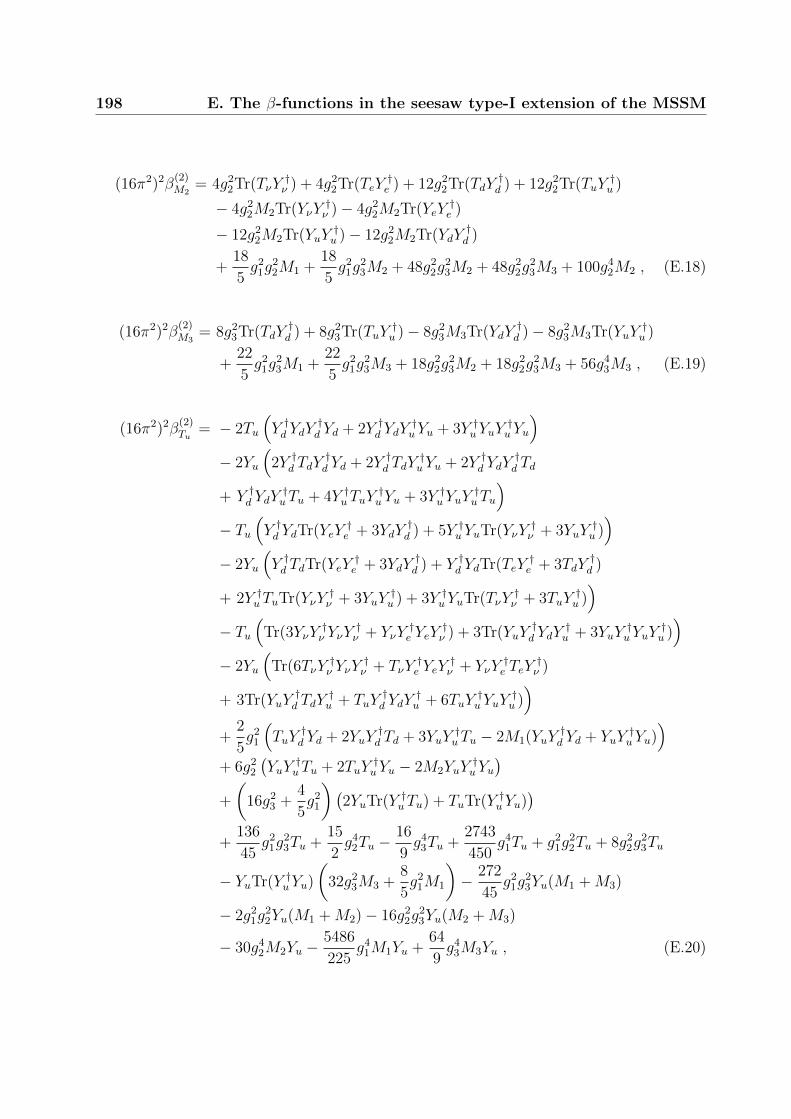
198 E. The β-functions in the seesaw type-I extension of the MSSM
(16π2)2β(2)M2
= 4g22Tr(TνY
†ν ) + 4g2
2Tr(TeY†e ) + 12g2
2Tr(TdY†d ) + 12g2
2Tr(TuY†u )
− 4g22M2Tr(YνY
†ν )− 4g2
2M2Tr(YeY†e )
− 12g22M2Tr(YuY
†u )− 12g2
2M2Tr(YdY†d )
+18
5g2
1g22M1 +
18
5g2
1g23M2 + 48g2
2g23M2 + 48g2
2g23M3 + 100g4
2M2 , (E.18)
(16π2)2β(2)M3
= 8g23Tr(TdY
†d ) + 8g2
3Tr(TuY†u )− 8g2
3M3Tr(YdY†d )− 8g2
3M3Tr(YuY†u )
+22
5g2
1g23M1 +
22
5g2
1g23M3 + 18g2
2g23M2 + 18g2
2g23M3 + 56g4
3M3 , (E.19)
(16π2)2β(2)Tu
= − 2Tu
(Y †d YdY
†d Yd + 2Y †d YdY
†uYu + 3Y †uYuY
†uYu
)− 2Yu
(2Y †d TdY
†d Yd + 2Y †d TdY
†uYu + 2Y †d YdY
†d Td
+ Y †d YdY†uTu + 4Y †uTuY
†uYu + 3Y †uYuY
†uTu
)− Tu
(Y †d YdTr(YeY
†e + 3YdY
†d ) + 5Y †uYuTr(YνY
†ν + 3YuY
†u ))
− 2Yu
(Y †d TdTr(YeY
†e + 3YdY
†d ) + Y †d YdTr(TeY
†e + 3TdY
†d )
+ 2Y †uTuTr(YνY†ν + 3YuY
†u ) + 3Y †uYuTr(TνY
†ν + 3TuY
†u ))
− Tu(
Tr(3YνY†ν YνY
†ν + YνY
†e YeY
†ν ) + 3Tr(YuY
†d YdY
†u + 3YuY
†uYuY
†u ))
− 2Yu
(Tr(6TνY
†ν YνY
†ν + TνY
†e YeY
†ν + YνY
†e TeY
†ν )
+ 3Tr(YuY†d TdY
†u + TuY
†d YdY
†u + 6TuY
†uYuY
†u ))
+2
5g2
1
(TuY
†d Yd + 2YuY
†d Td + 3YuY
†uTu − 2M1(YuY
†d Yd + YuY
†uYu)
)+ 6g2
2
(YuY
†uTu + 2TuY
†uYu − 2M2YuY
†uYu
)+
(16g2
3 +4
5g2
1
)(2YuTr(Y †uTu) + TuTr(Y †uYu)
)+
136
45g2
1g23Tu +
15
2g4
2Tu −16
9g4
3Tu +2743
450g4
1Tu + g21g
22Tu + 8g2
2g23Tu
− YuTr(Y †uYu)
(32g2
3M3 +8
5g2
1M1
)− 272
45g2
1g23Yu(M1 +M3)
− 2g21g
22Yu(M1 +M2)− 16g2
2g23Yu(M2 +M3)
− 30g42M2Yu −
5486
225g4
1M1Yu +64
9g4
3M3Yu , (E.20)

E.2 Two-Loop β-functions 199
(16π2)2β(2)Td
= − 2Td
(3Y †d YdY
†d Yd + 2Y †uYuY
†d Yd + Y †uYuY
†uYu
)− 2Yd
(4Y †d TdY
†d Yd + 3Y †d YdY
†d Td + 2Y †uTuY
†d Yd
+ 2Y †uTuY†uYu + Y †uYuY
†d Td + 2Y †uYuY
†uTu
)− Td
(5Y †d YdTr(YeY
†e + 3YdY
†d ) + Y †uYuTr(YνY
†ν + 3YuY
†u ))
− 2Yd
(2Y †d TdTr(YeY
†e + 3YdY
†d ) + 3Y †d YdTr(TeY
†e + 3TdY
†d )
+ Y †uTuTr(YνY†ν + 3YuY
†u ) + Y †uYuTr(TνY
†ν + 3TuY
†u ))
− Td(
Tr(YeY†ν YνY
†e + 3YeY
†e YeY
†e ) + 3Tr(YuY
†d YdY
†u + 3YdY
†d YdY
†d ))
− 2Yd
(Tr(YeY
†ν TνY
†e + TeY
†ν YνY
†e + 6TeY
†e YeY
†e )
+ 3Tr(TdY†uYuY
†d + TuY
†d YdY
†u + 6TdY
†d YdY
†d ))
+2
5g2
1
(2TdY
†uYu + 3TdY
†d Yd + 3YdY
†d Td + 4YdY
†uTu − 4M1(YdY
†d Yd + YdY
†uYu)
)+ 6g2
2
(YdY
†d Td + 2TdY
†d Yd − 2M2YdY
†d Yd
)+
(16g2
3 −2
5g2
1
)(2YdTr(Y †d Td) + TdTr(Y †d Yd)
)+
6
5g2
1
(2YdTr(Y †e Te) + TdTr(Y †e Ye)
)+
8
9g2
1g23Td +
15
2g4
2Td −16
9g4
3Td +287
90g4
1Td + g21g
22Td + 8g2
2g23Td
− YdTr(Y †d Yd)
(32g2
3M3 −4
5g2
1M1
)− 12
5g2
1M1YdTr(Y †e Ye)
− 16
9g2
1g23Yd(M1 +M3)− 2g2
1g22Yd(M1 +M2)− 16g2
2g23Yd(M2 +M3)
− 30g42M2Yd −
574
45g4
1M1Yd +64
9g4
3M3Yd , (E.21)
(16π2)2β(2)Te
= − 2Te
(3Y †e YeY
†e Ye + 2Y †ν YνY
†e Ye + Y †ν YνY
†ν Yν
)− 2Ye
(4Y †e TeY
†e Ye + 3Y †e YeY
†e Te + 2Y †ν TνY
†e Ye
+ 2Y †ν TνY†ν Yν + Y †ν YνY
†e Te + 2Y †ν YνY
†ν Tν
)− Te
(5Y †e YeTr(YeY
†e + 3YdY
†d ) + Y †ν YνTr(YνY
†ν + 3YuY
†u ))
− 2Ye
(2Y †e TeTr(YeY
†e + 3YdY
†d ) + 3Y †e YeTr(TeY
†e + 3TdY
†d )

200 E. The β-functions in the seesaw type-I extension of the MSSM
+ Y †ν TνTr(YνY†ν + 3YuY
†u ) + Y †ν YνTr(TνY
†ν + 3TuY
†u ))
− Te(
Tr(YeY†ν YνY
†e + 3YeY
†e YeY
†e ) + 3Tr(YdY
†uYuY
†d + 3YdY
†d YdY
†d ))
− 2Ye
(Tr(YeY
†ν TνY
†e + TeY
†ν YνY
†e + 6TeY
†e YeY
†e )
+ 3Tr(TdY†uYuY
†d + TuY
†d YdY
†u + 6TdY
†d YdY
†d ))
+6
5g2
1
(YeY
†e Te − TeY †e Ye
)+ 6g2
2
(YeY
†e Te + 2TeY
†e Ye − 2M2YeY
†e Ye)
+
(16g2
3 −2
5g2
1
)(2YeTr(Y †d Td) + TeTr(Y †d Yd)
)+
6
5g2
1
(2YeTr(Y †e Te) + TeTr(Y †e Ye)
)+
15
2g4
2Te +27
2g4
1Te +9
5g2
1g22Te
− YeTr(Y †d Yd)
(32g2
3M3 −4
5g2
1M1
)− 12
5g2
1M1YeTr(Y †e Ye)
− 18
5g2
1g22Yd(M1 +M2)− 30g4
2M2Ye − 54g41M1Ye , (E.22)
(16π2)2β(2)Tν
= − 2Tν
(Y †e YeY
†e Ye + 2Y †e YeY
†ν Yν + 3Y †ν YνY
†ν Yν
)− 2Yν
(2Y †e TeY
†e Ye + 2Y †e TeY
†ν Yν + 2Y †e YeY
†e Te
+ Y †e YeY†ν Tν + 4Y †ν TνY
†ν Yν + 3Y †ν YνY
†ν Tν
)− Tν
(Y †e YeTr(YeY
†e + 3YdY
†d ) + 5Y †ν YνTr(YνY
†ν + 3YuY
†u ))
− 2Yν
(Y †e TeTr(YeY
†e + 3YdY
†d ) + Y †e YeTr(TeY
†e + 3TdY
†d )
+ 2Y †ν TνTr(YνY†ν + 3YuY
†u ) + 3Y †ν YνTr(TνY
†ν + 3TuY
†u ))
− Tν(
Tr(3YνY†ν YνY
†ν + YνY
†e YeY
†ν ) + 3Tr(YuY
†d YdY
†u + 3YuY
†uYuY
†u ))
− 2Yν
(Tr(TνY
†e YeY
†ν + YνY
†e TeY
†ν + 6TνY
†ν YνY
†ν )
+ 3Tr(TdY†uYuY
†d + TuY
†d YdY
†u + 6TuY
†uYuY
†u ))
+6
5g2
1
(2TνY
†ν Yν + 2YνY
†e Te + YνY
†ν Tν + TνY
†e Ye − 2M1(YνY
†ν Yν + YνY
†e Ye)
)+ 6g2
2
(YνY
†ν Tν + 2TνY
†ν Yν − 2M2YνY
†ν Yν)
+
(16g2
3 +4
5g2
1
)(2YνTr(Y †uTu) + TνTr(Y †uYu)
)

E.2 Two-Loop β-functions 201
+15
2g4
2Tν +207
50g4
1Tν +9
5g2
1g22Tν
− YνTr(Y †uYu)
(32g2
3M3 +8
5g2
1M1
)− 18
5g2
1g22Yν(M1 +M2)− 30g4
2M2Yν −414
25g4
1M1Yν , (E.23)
(16π2)2β(2)
m2L
= − 4T †e
(TeY
†e Ye + YeY
†e Te
)− 4T †ν
(TνY
†ν Yν + YνY
†ν Tν
)− 2Y †e
(2m2
eYeY†e Ye + 2TeT
†eYe + 2YeT
†eTe
+2YeY†em
2eYe + YeY
†e Yem
2L
+ 2Yem2LY †e Ye
)− 2Y †ν
(2m2
νYνY†ν Yν + 2TνT
†νYν + 2YνT
†νTν
+2YνY†νm
2νYν + YνY
†ν Yνm
2L
+ 2Yνm2LY †ν Yν
)− 2
(4m2
hd+m2
L
)Y †e YeY
†e Ye − 2
(4m2
hu +m2L
)Y †ν YνY
†ν Yν
− 2T †e
(TeTr(YeY
†e + 3YdY
†d ) + YeTr(TeY
†e + 3TdY
†d ))
− 2T †ν
(TνTr(YνY
†ν + 3YuY
†u ) + YνTr(TνY
†ν + 3TuY
†u ))
− Y †e(
2m2eYeTr(YeY
†e + 3YdY
†d ) + 2TeTr(YeT
†e + 3YdT
†d )
+ 2YeTr(TeT†e + 3TdT
†d ) + Yem
2LTr(YeY
†e + 3YdY
†d ))
− Y †ν(
2m2νYνTr(YνY
†ν + 3YuY
†u ) + 2TνTr(YνT
†ν + 3YuT
†u)
+ 2YνTr(TνT†ν + 3TuT
†u) + Yνm
2LTr(YνY
†ν + 3YuY
†u ))
−(
4m2hd
+m2L
)Y †e YeTr(YeY
†e + 3YdY
†d )
−(
4m2hu +m2
L
)Y †ν YνTr(YνY
†ν + 3YuY
†u )
− 2Y †e YeTr(Yem
2LY †e + Y †em
2eYe + 3Ydm
2QY †d + 3Y †dm
2dYd
)− 2Y †ν YνTr
(Yνm
2LY †ν + Y †νm
2νYν + 3Yum
2QY †u + 3Y †um
2uYu
)+
6
5g2
1
(2m2
hdY †e Ye +m2
LY †e Ye + Y †e Yem
2L
+ 2Y †em2eYe + 2T †eTe
)− 12
5g2
1
(M∗
1Y†e Te − 2|M1|2Y †e Ye +M1T
†eYe)
+621
25g4
1|M1|2 13 +18
5g2
1g22(|M1|2 + |M2|2) 13
+18
5g2
1g22Re(M1M
∗2 ) 13 + 33g4
2|M2|2 13

202 E. The β-functions in the seesaw type-I extension of the MSSM
+3
5g2
1σ1 13 + 3g22σ2 13 −
6
5g2
1S′ 13 , (E.24)
(16π2)2β(2)
m2Q
= − 4T †d
(TdY
†d Yd + YdY
†d Td
)− 4T †u
(TuY
†uYu + YuY
†uTu
)− 2Y †d
(2m2
dYdY
†d Yd + 2TdT
†dYd + 2YdT
†dTd
+2YdY†dm
2dYd + YdY
†d Ydm
2Q
+ 2Ydm2QY †d Yd
)− 2Y †u
(2m2
uYuY†uYu + 2TuT
†uYu + 2YuT
†uTu
+2YuY†um
2uYu + YuY
†uYum
2Q
+ 2Yum2QY †uYu
)− 2
(4m2
hd+m2
Q
)Y †d YdY
†d Yd − 2
(4m2
hu +m2Q
)Y †uYuY
†uYu
− 2T †d
(TdTr(YeY
†e + 3YdY
†d ) + YdTr(TeY
†e + 3TdY
†d ))
− 2T †u
(TuTr(YνY
†ν + 3YuY
†u ) + YuTr(TνY
†ν + 3TuY
†u ))
− Y †d(
2m2dYdTr(YeY
†e + 3YdY
†d ) + 2TdTr(YeT
†e + 3YdT
†d )
+ 2YdTr(TeT†e + 3TdT
†d ) + Ydm
2Q
Tr(YeY†e + 3YdY
†d ))
− Y †u(
2m2uYuTr(YνY
†ν + 3YuY
†u ) + 2TuTr(YνT
†ν + 3YuT
†u)
+ 2YuTr(TνT†ν + 3TuT
†u) + Yum
2Q
Tr(YνY†ν + 3YuY
†u ))
−(
4m2hd
+m2Q
)Y †d YdTr(YeY
†e + 3YdY
†d )
−(
4m2hu +m2
Q
)Y †uYuTr(YνY
†ν + 3YuY
†u )
− 2Y †d YdTr(Yem
2LY †e + Y †em
2eYe + 3Ydm
2QY †d + 3Y †dm
2dYd
)− 2Y †uYuTr
(Yνm
2LY †ν + Y †νm
2νYν + 3Yum
2QY †u + 3Y †um
2uYu
)+
2
5g2
1
(2m2
hdY †d Yd + 4m2
huY†uYu +m2
QY †d Yd + Y †d Ydm
2Q
+ 2Y †dm2dYd
+ 2m2QY †uYu + 2Y †uYum
2Q
+ 4Y †um2uYu + 2T †dTd + 4T †uTu
)− 4
5g2
1
(M∗
1Y†d Td + 2M∗
1Y†uTu − 4|M1|2Y †uYu
+ M1T†dYd + 2M1T
†uYu − 2|M1|2Y †d Yd
)− 128
3g4
3|M3|2 13 +2
5g2
1g22Re (M1M
∗2 ) 13 +
32
45g2
1g23Re (M1M
∗3 ) 13
+199
75g4
1|M1|2 13 +2
5g2
1g22(|M1|2 + |M2|2) 13

E.2 Two-Loop β-functions 203
+ 32g22g
23(|M2|2 +Re(M2M
∗3 ) + |M3|2) 13
+32
45g2
1g23(|M1|2 + |M3|2) 13 + 33g4
2|M2|2 13
+1
15g2
1σ1 13 + 3g22σ2 13 +
16
3g2
3σ3 13 +2
5g2
1S′ 13 , (E.25)
(16π2)2β(2)
m2u
= − 2(
2m2hd
+ 2m2hu +m2
u
)YuY
†d YdY
†u − 2
(4m2
hu +m2u
)YuY
†uYuY
†u
− 4Tu
(T †dYdY
†u + T †uYuY
†u + Y †d YdT
†u + Y †uYuT
†u
)− 4Yu
(T †dTdY
†u + T †uTuY
†u + Y †d TdT
†u + Y †uTuT
†u
)− 2Yu
(2Y †dm
2dYdY
†u + Y †d YdY
†um
2u + 2Y †d Ydm
2QY †u + 2Y †um
2uYuY
†u
+ Y †uYuY†um
2u + 2Y †uYum
2QY †u + 2m2
QY †d YdY
†u + 2m2
QY †uYuY
†u
)− 2
(4m2
hu +m2u
)YuY
†uTr(YνY
†ν + 3YuY
†u )
− 4Tu
(T †uTr(YνY
†ν + 3YuY
†u ) + Y †uTr(YνT
†ν + 3YuT
†u))
− 4Yu
(T †uTr(TνY
†ν + 3TuY
†u ) + Y †uTr(TνT
†ν + 3TuT
†u))
− 2Y †u
(Y †um
2uTr(YνY
†ν + 3YuY
†u ) + 2m2
QY †uTr(YνY
†ν + 3YuY
†u )
+ 2Y †uTr(Yνm2LY †ν + Y †νm
2νYν + 3Yum
2QY †u + 3Y †um
2uYu)
)+
(6g2
2 −2
5g2
1
)(m2uYuY
†u + YuY
†um
2u + 2m2
huYuY†u + 2Yum
2QY †u + 2TuT
†u
)− 12g2
2
(M∗
2TuY†u − 2|M2|2YuY †u +M2YuT
†u
)+
4
5g2
1
(M∗
1TuY†u − 2|M1|2YuY †u +M1YuT
†u
)− 128
3g4
3|M3|2 13 +512
45g2
1g23
(|M1|2 +Re(M1M
∗3 ) + |M3|2
)13
+3424
75g4
1|M1|2 13 +16
15g2
1σ1 13 +16
3g2
3σ3 13 −8
5g2
1S′ 13 , (E.26)
(16π2)2β(2)
m2d
= − 2(
2m2hd
+ 2m2hu +m2
d
)YdY
†uYuY
†d − 2
(4m2
hd+m2
d
)YdY
†d YdY
†d
− 4Td
(T †dYdY
†d + T †uYuY
†d + Y †d YdT
†d + Y †uYuT
†d
)− 4Yd
(T †dTdY
†d + T †uTuY
†d + Y †d TdT
†d + Y †uTuT
†d
)− 2Yd
(2Y †dm
2dYdY
†d + Y †d YdY
†dm
2d
+ 2Y †d Ydm2QY †d + 2Y †um
2uYuY
†d

204 E. The β-functions in the seesaw type-I extension of the MSSM
+ Y †uYuY†dm
2d
+ 2Y †uYum2QY †d + 2m2
QY †d YdY
†d + 2m2
QY †uYuY
†d
)− 2
(4m2
hd+m2
d
)YdY
†d Tr(YeY
†e + 3YdY
†d )
− 4Td
(T †dTr(YeY
†e + 3YdY
†d ) + Y †d Tr(YeT
†e + 3YdT
†d ))
− 4Yd
(T †dTr(TeY
†e + 3TdY
†d ) + Y †d Tr(TeT
†e + 3TdT
†d ))
− 2Y †d
(Y †dm
2dTr(YeY
†e + 3YdY
†d ) + 2m2
QY †d Tr(YeY
†e + 3YdY
†d )
+ 2Y †d Tr(Yem2LY †e + Y †em
2eYe + 3Ydm
2QY †d + 3Y †dm
2dYd))
+
(6g2
2 +2
5g2
1
)(m2dYdY
†d + YdY
†dm
2d
+ 2m2hdYdY
†d + 2Ydm
2QY †d + 2TdT
†d
)− 12g2
2
(M∗
2TdY†d − 2|M2|2YdY †d +M2YdT
†d
)− 4
5g2
1
(M∗
1TdY†d − 2|M1|2YdY †d +M1YdT
†d
)− 128
3g4
3|M3|2 13 +128
45g2
1g23
(|M1|2 +Re(M1M
∗3 ) + |M3|2
)13
+808
75g4
1|M1|2 13 +4
15g2
1σ1 13 +16
3g2
3σ3 13 +4
5g2
1S′ 13 , (E.27)
(16π2)2β(2)
m2e
= − 2(
2m2hd
+ 2m2hu +m2
e
)YeY
†ν YνY
†e − 2
(4m2
hd+m2
e
)YeY
†e YeY
†e
− 4Te
(T †eYeY
†e + T †νYνY
†e + Y †e YeT
†e + Y †ν YνT
†e
)− 4Ye
(T †eTeY
†e + T †νTνY
†e + Y †e TeT
†e + Y †ν TνT
†e
)− 2Ye
(2Y †em
2eYeY
†e + Y †e YeY
†em
2e + 2Y †e Yem
2LY †e + 2Y †νm
2νYνY
†e
+ Y †ν YνY†em
2e + 2Y †ν Yνm
2LY †e + 2m2
LY †e YeY
†e + 2m2
LY †ν YνY
†e
)− 2
(4m2
hd+m2
e
)YeY
†e Tr(YeY
†e + 3YdY
†d )
− 4Te
(T †eTr(YeY
†e + 3YdY
†d ) + Y †e Tr(YeT
†e + 3YdT
†d ))
− 4Ye
(T †eTr(TeY
†e + 3TdY
†d ) + Y †e Tr(TeT
†e + 3TdT
†d ))
− 2Y †e
(Y †em
2eTr(YeY
†e + 3YdY
†d ) + 2m2
LY †e Tr(YeY
†e + 3YdY
†d )
+ 2Y †e Tr(Yem2LY †e + Y †em
2eYe + 3Ydm
2QY †d + 3Y †dm
2dYd))
+
(6g2
2 −6
5g2
1
)(m2eYeY
†e + YeY
†em
2e + 2m2
hdYeY
†e + 2Yem
2LY †e + 2TeT
†e
)− 12g2
2
(M∗
2TeY†e − 2|M2|2YeY †e +M2YeT
†e
)

E.2 Two-Loop β-functions 205
+12
5g2
1
(M∗
1TeY†e − 2|M1|2YeY †e +M1YeT
†e
)+
2808
25g4
1|M1|2 13 +12
5g2
1σ1 13 +12
5g2
1S′ 13 , (E.28)
(16π2)2β(2)
m2ν
= − 2(
2m2hd
+ 2m2hu +m2
ν
)YνY
†e YeY
†ν − 2
(4m2
hu +m2ν
)YνY
†ν YνY
†ν
− 4Tν
(T †eYeY
†ν + T †νYνY
†ν + Y †e YeT
†ν + Y †ν YνT
†ν
)− 4Yν
(T †eTeY
†ν + T †νTνY
†ν + Y †e TeT
†ν + Y †ν TνT
†ν
)− 2Yν
(2Y †em
2eYeY
†ν + Y †e YeY
†νm
2ν + 2Y †e Yem
2LY †ν + 2Y †νm
2νYνY
†ν
+ Y †ν YνY†νm
2ν + 2Y †ν Yνm
2LY †ν + 2m2
LY †e YeY
†ν + 2m2
LY †ν YνY
†ν
)− 2
(4m2
hu +m2ν
)YνY
†ν Tr(YνY
†ν + 3YuY
†u )
− 4Tν
(T †νTr(YνY
†ν + 3YuY
†u ) + Y †ν Tr(YνT
†ν + 3YuT
†u))
− 4Yν
(T †νTr(TνY
†ν + 3TuY
†u ) + Y †ν Tr(TνT
†ν + 3TuT
†u))
− 2Y †ν
(Y †νm
2νTr(YνY
†ν + 3YuY
†u ) + 2m2
LY †ν Tr(YνY
†ν + 3YuY
†u )
+ 2Y †ν Tr(Yνm2LY †ν + Y †νm
2νYν + 3Yum
2QY †u + 3Y †um
2uYu)
)+
(6g2
2 +6
5g2
1
)(m2νYνY
†ν + YνY
†νm
2ν + 2m2
huYνY†ν + 2Yνm
2LY †ν + 2TνT
†ν
)− 12g2
2
(M∗
2TνY†ν − 2|M2|2YνY †ν +M2YνT
†ν
)− 12
5g2
1
(M∗
1TνY†ν − 2|M1|2YνY †ν +M1YνT
†ν
), (E.29)
(16π2)2β(2)
m2hd
= − 2(m2hd
+m2hu
)Tr(YeY
†ν YνY
†e + 3YdY
†uYuY
†d )
− 12m2hd
Tr(YeY†e YeY
†e + 3YdY
†d YdY
†d )
− 12Tr(T †eTeY†e Ye + 3T †dTdY
†d Yd + T †eYeY
†e Te + 3T †dYdY
†d Td)
− 2Tr(TeT†νYνY
†e + 3TdT
†uYuY
†d + TeY
†ν YνT
†e + 3TdY
†uYuT
†d )
− 2Tr(YeT†νTνY
†e + 3YdT
†uTuY
†d + YeY
†ν TνT
†e + 3YdY
†uTuT
†d )
− 36Tr(YdY†dm
2dYdY
†d + Y †d Ydm
2QY †d Yd)
− 12Tr(YeY†em
2eYeY
†e + Y †e Yem
2LY †e Ye)
− 6Tr(YuY†dm
2dYdY
†u + YdY
†um
2uYuY
†d + Y †uYum
2QY †d Yd + Y †d Ydm
2QY †uYu)
− 2Tr(YνY†em
2eYeY
†ν + YeY
†νm
2νYνY
†e + Y †ν Yνm
2LY †e Ye + Y †e Yem
2LY †ν Yν)

206 E. The β-functions in the seesaw type-I extension of the MSSM
+
(32g2
3 −4
5g2
1
)Tr(T †dTd +m2
hdY †d Yd + Ydm
2QY †d + Y †dm
2dYd)
+12
5g2
1Tr(T †eTe +m2hdY †e Ye + Yem
2LY †e + Y †em
2eYe)
− 12
5g2
1Tr(M∗1Y†e Te +M1T
†eYe − 2|M1|2Y †e Ye)
+4
5g2
1Tr(M∗1Y†d Td +M1T
†dYd − 2|M1|2Y †d Yd)
− 32g23Tr(M∗
3Y†d Td +M3T
†dYd − 2|M3|2Y †d Yd)
+18
5g2
1g22
(|M1|2 +Re(M1M
∗2 ) + |M2|2
)+
621
25g4
1|M1|2 + 33g42|M2|2 +
3
5g2
1σ1 + 3g22σ2 −
6
5g2
1S′ , (E.30)
(16π2)2β(2)
m2hu
= − 2(m2hd
+m2hu
)Tr(YeY
†ν YνY
†e + 3YdY
†uYuY
†d )
− 12m2huTr(YνY
†ν YνY
†ν + 3YuY
†uYuY
†u )
− 12Tr(T †νTνY†ν Yν + 3T †uTuY
†uYu + T †νYνY
†ν Tν + 3T †uYuY
†uTu)
− 2Tr(TeT†νYνY
†e + 3TdT
†uYuY
†d + TeY
†ν YνT
†e + 3TdY
†uYuT
†d )
− 2Tr(YeT†νTνY
†e + 3YdT
†uTuY
†d + YeY
†ν TνT
†e + 3YdY
†uTuT
†d )
− 36Tr(YuY†um
2uYuY
†u + Y †uYum
2QY †uYu)
− 12Tr(YνY†νm
2νYνY
†ν + Y †ν Yνm
2LY †ν Yν)
− 6Tr(YuY†dm
2dYdY
†u + YdY
†um
2uYuY
†d + Y †uYum
2QY †d Yd + Y †d Ydm
2QY †uYu)
− 2Tr(YνY†em
2eYeY
†ν + YeY
†νm
2νYνY
†e + Y †ν Yνm
2LY †e Ye + Y †e Yem
2LY †ν Yν)
+
(32g2
3 +8
5g2
1
)Tr(T †uTu +m2
huY†uYu + Yum
2QY †u + Y †um
2uYu)
− 8
5g2
1Tr(M∗1Y†uTu +M1T
†uYu − 2|M1|2Y †uYu)
− 32g23Tr(M∗
3Y†uTu +M3T
†uYu − 2|M3|2Y †uYu)
+18
5g2
1g22
(|M1|2 +Re(M1M
∗2 ) + |M2|2
)+
621
25g4
1|M1|2 + 33g42|M2|2 +
3
5g2
1σ1 + 3g22σ2 +
6
5g2
1S′ , (E.31)
with
σ1 =1
5g2
1
(3m2
hu + 3m2hd
+ Tr(m2Q
+ 3m2L
+ 2m2d
+ 6m2e + 8m2
u
)), (E.32)
σ22 = g2
2
(m2hu +m2
hd+ Tr
(3m2
Q+m2
L
)), (E.33)
σ3 = g23Tr
(2m2
Q+m2
d+m2
u
), (E.34)

E.2 Two-Loop β-functions 207
and
S ′ = m2hd
Tr(YeY
†e + 3YdY
†d
)−m2
huTr(YνY
†ν + 3YuY
†u
)+ Tr
(m2LY †e Ye +m2
LY †ν Yν
)− Tr
(m2QY †d Yd +m2
QY †uYu
)− 2Tr
(YdY
†dm
2d
+ YeY†em
2e − 2YuY
†um
2u
)+
1
30g2
1
(9m2
hu − 9m2hd
+ Tr(m2Q− 9m2
L+ 4m2
d+ 36m2
e − 32m2u
))+
3
2g2
2
(m2hu −m2
hd+ Tr
(m2Q−m2
L
))+
8
3g2
3Tr(m2Q
+m2d− 2m2
u
). (E.35)
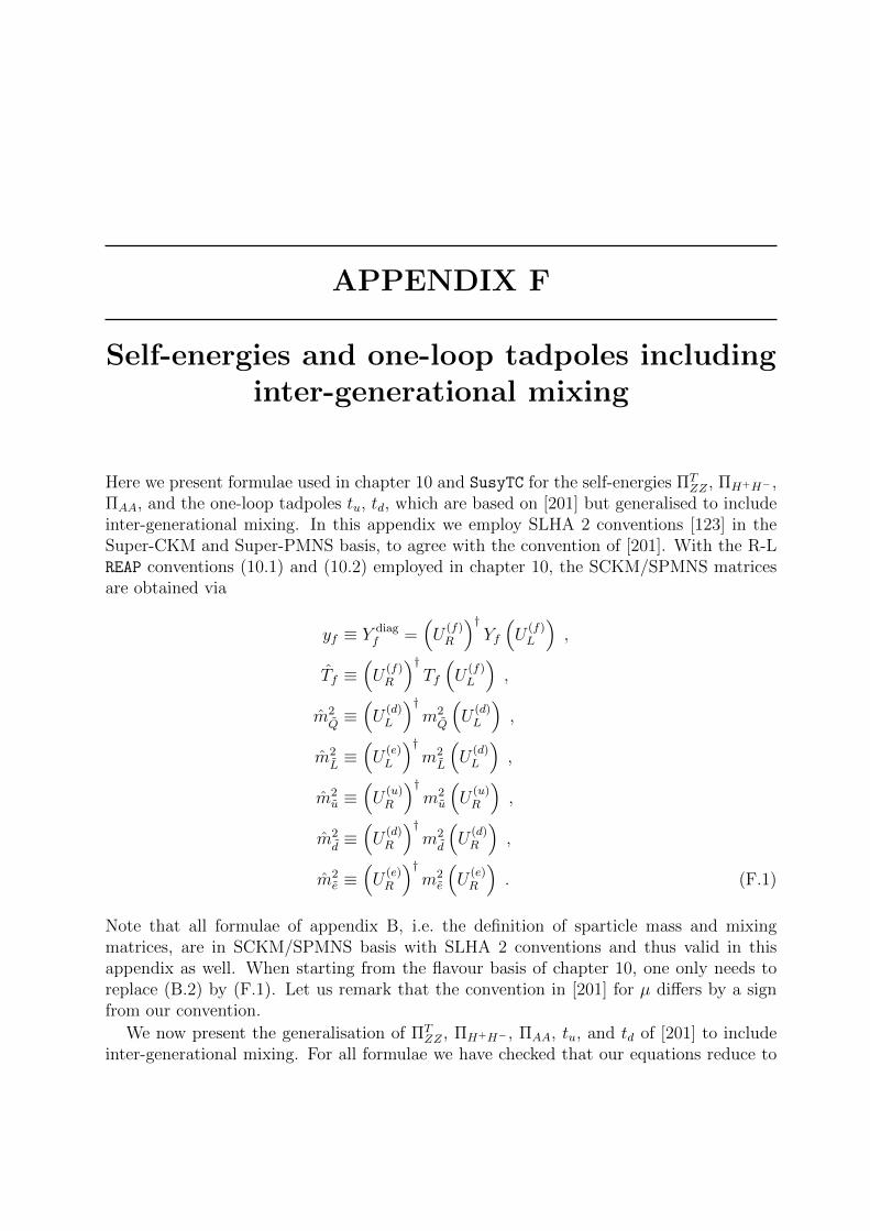
APPENDIX F
Self-energies and one-loop tadpoles includinginter-generational mixing
Here we present formulae used in chapter 10 and SusyTC for the self-energies ΠTZZ , ΠH+H− ,
ΠAA, and the one-loop tadpoles tu, td, which are based on [201] but generalised to includeinter-generational mixing. In this appendix we employ SLHA 2 conventions [123] in theSuper-CKM and Super-PMNS basis, to agree with the convention of [201]. With the R-LREAP conventions (10.1) and (10.2) employed in chapter 10, the SCKM/SPMNS matricesare obtained via
yf ≡ Y diagf =
(U
(f)R
)†Yf
(U
(f)L
),
Tf ≡(U
(f)R
)†Tf
(U
(f)L
),
m2Q≡(U
(d)L
)†m2Q
(U
(d)L
),
m2L≡(U
(e)L
)†m2L
(U
(d)L
),
m2u ≡
(U
(u)R
)†m2u
(U
(u)R
),
m2d≡(U
(d)R
)†m2d
(U
(d)R
),
m2e ≡
(U
(e)R
)†m2e
(U
(e)R
). (F.1)
Note that all formulae of appendix B, i.e. the definition of sparticle mass and mixingmatrices, are in SCKM/SPMNS basis with SLHA 2 conventions and thus valid in thisappendix as well. When starting from the flavour basis of chapter 10, one only needs toreplace (B.2) by (F.1). Let us remark that the convention in [201] for µ differs by a signfrom our convention.
We now present the generalisation of ΠTZZ , ΠH+H− , ΠAA, tu, and td of [201] to include
inter-generational mixing. For all formulae we have checked that our equations reduce to

209
the corresponding equations in [201] when
Wfi i= Wfi+3 i+3
= cos θfiWfi i+3
= −Wfi+3 i= − sin θfi , (F.2)
where i = 1 . . . 3 and Wf is defined in (B.6).We keep the abbreviations of [201]:
sαβ ≡ sin(α− β) , (F.3)
cαβ ≡ cos(α− β) , (F.4)
gfL ≡ I3 −Qe sin2 θW , (F.5)
gfR ≡ Qe sin2 θW , (F.6)
e ≡ g2 sin θW , (F.7)
NC ≡
3 for (s)quarks
1 for (s)fermions. (F.8)
The conventions for the one-loop scalar functions A0, B22, B22, H, G, and F [220] areadopted from appendix B of [201]. Summations
∑f are over all fermions, whereas sum-
mations∑
fu,∑
fdare restricted to up-type and down-type fermions, respectively. Sum-
mations∑
Q,∑
Q are over SU(2) (s)quark doublets, and analogously for (s)leptons. In
summations over sfermions the indices i, j, s, and t run from 1 to 6 for u, d, and e and from1 to 3 for ν. In summations of neutralinos (charginos) the indices i, j run from 1 to 4 (2).The summation
∑h0 runs over all neutral Higgs- and Goldstone bosons, the summation∑
h+ over the charged ones.
16π2 cos2 θWg2
2
ΠTZZ(p2) =− s2
αβ
(B22(mA,mH) + B22(MZ ,mh)−M2
ZB0(MZ ,mh))
− c2αβ
(B22(MZ ,mH) + B22(mA,mh)−M2
ZB0(MZ ,mh))
− 2 cos4 θW
(2p2 +M2
W −M2Z
sin4 θWcos2 θW
)B0(MW ,MW )
−(8 cos4 θW + cos2(2θW )
)B22(MW ,MW )
− cos2(2θW )B22(mH+ ,mH+)
−∑f
NC
∑s,t
∣∣∣∣∣I3
∑i
W ∗fisWfit
−Qe sin2 θW δst
∣∣∣∣∣2
4B22(mfs,mft
)
+1
2
∑f
NC
∑s
((1− 8I3Qe sin2 θW )
∑i
W ∗fisWfis
+ 4Q2e sin4 θW
)A0(mfs
)

210 F. Self-energies and one-loop tadpoles including inter-generational mixing
+∑f
NC
((g2fL
+ g2fR
)H(mf ,mf )− 4gfLgfRm
2fB0(mf ,mf )
)+
cos2 θW2g2
2
∑i,j
f 0ijZH(mχ0
i,mχ0
j) + 2g0
ijZmχ0imχ0
jB0(mχ0
i,mχ0
j)
+cos2 θWg2
2
∑i,j
f+ijZH(mχ+
i,mχ+
j) + 2g+
ijZmχ+imχ+
jB0(mχ+
i,mχ+
j) .
(F.9)
The couplings f 0Z , f+
Z , g0Z , and g+
Z are given in Eqs. (A.7) and (D.5) of [201].
16π2ΠH+H−(p2) =∑Q
NC
((cos2 βy2
u + sin2 βy2d
)G(mu,md)
− 2 sin(2β)yuydmumdB0(mu,md)
)+∑L
sin2 βy2eG(0,me)
+∑Q
NC
∑i,j
(λH+Q
)2
ijB0(mui ,mdj
)
+∑L
∑i,j
(λH+L)2ij B0(mνi ,mej)
+∑f
∑i
(λH+H−f
)iiA0(mfi
)
+g2
2
4
(s2αβF (mH ,MW ) + c2
αβF (mh,MW ) + F (mA,MW )
+cos2(2θW )
cos2 θWF (mH+ ,MZ)
)+ e2F (mH+ , 0) + 2g2
2A0(MW ) + g22 cos2(2θW )A0(MZ)
+∑h+
(∑h0
(λH+h0h−)2B0(mh0 ,mh+) + λH+H−h+h−A0(mh+)
)
+ g22
M2W
4B0(MW ,mA)
+1
2
∑h0
λH+H−h0h0A0(mh0)
+∑j,i
fijH+G(mχ+j,mχ0
i)− 2mχ+
jmχ0
igijH+B0(mχ+
j,mχ0
i) . (F.10)
The couplings fH+ and gH+ are given in Eq. (D.70) and Eqs. (D.39-D.42) of [201]. The cou-

211
plings λH+H−h− , λH+H−h+h− , and λH+H−h0h0 are defined in Eqs. (D.63-D.65) and Eq. (D.67)of [201]. The couplings to sfermions in the case of inter-generational mixing are given by
λH+Q = Wu
(g2√
2MW sin(2β) 13 − (y2
u + y2d) cos β v sinβ√
2−T †d sin β − µyd cos β
−Tu cos β − µ∗yu sin β −yuyd v√2
)Wd ,
(F.11)
λH+L = Wν
(g2√
2MW sin(2β) 13 − y2
e cos β v sinβ√2
−T †e sin β − µye cos β)We , (F.12)
λH+H−f = −W †f
(−g2
2
2cos(2β)
(cos(2θW )cos2 θW
I3 + tan2 θWQe
)13 0
0g22
2cos(2β) tan2 θWQe 13
)Wf
+
W †u
(y2d sin2 β 0
0 y2u cos2 β
)Wu f = u
W †d
(y2u cos2 β 0
0 y2d sin2 β
)Wd f = d
W †e
(0 0
0 y2e sin2 β
)We f = e
, (F.13)
λH+H−ν = −W †ν
(−g
22
2cos(2β)
(cos(2θW )
cos2 θWI3 + tan2 θWQe
)13 − y2
e sin2 β
)Wν (F.14)
16π2ΠAA(p2) = cos2 β∑fu
NCy2fu
(p2B0(mfu ,mfu)− 2A0(mfu)
)+ sin2 β
∑fd
NCy2fd
(p2B0(mfd ,mfd)− 2A0(mfd)
)+∑f
∑i
NC
((λAAf
)iiA0(mfi
) +∑j
(λAf
)2
ijB0(mfi
,mfj)
)
+g2
2
4
(2F (mH+ ,MW ) +
s2αβ
cos2 θWF (mH ,MZ) +
c2αβ
cos2 θWF (mh,MZ)
)
+1
2
∑h0n
∑h0m
λAh0nh
0mB0(mh0
n,mh0
m) + λAAh0
nh0nA0(mh0
n)
+ g2
2
(M2
W
2B0(MW ,mHp) + 2A0(MW ) +
1
cos2 θWA0(MZ)
)+∑h+
λAAh+h+A0(mh+)

212 F. Self-energies and one-loop tadpoles including inter-generational mixing
+1
2
∑i,j
f 0ijAG(mχ0
i,mχ0
j)− 2g0
ijAmχ0imχ0
jB0(mχ0
i,mχ0
j)
+∑i,j
f+ijAG(mχ+
i,mχ+
j)− 2g+
ijAmχ+imχ+
jB0(mχ+
i,mχ+
j) . (F.15)
The couplings f 0A, g0
A, f+A , and g+
A are given in Eq. (D.70) and Eqs. (D.34-D.38) of [201].The couplings λAh0h0 , λAAh0h0 , and λAAh+h+ are defined in Eqs. (D.63-D.65) and Eq. (D.67)of [201]. The couplings to sfermions in the case of inter-generational mixing are given by
λAu = W †u
0 − 1√2
(T †u cos β + µyu sin β
)1√2
(Tu cos β + µ∗yu sin β
) Wu , (F.16)
λAe(d) = W †e(d)
0 − 1√2
(T †e(d) sin β + µye(d) cos β
)1√2
(Te(d) sin β + µ∗ye(d) cos β
) We(d) ,
(F.17)
λAν = 0 , (F.18)
λAAf = W †f
(−g2
2
2cos(2β)
(1
cos2 θWI3 − tan2 θWQe
)13 0
0 −g22
2cos(2β) tan2 θWQe 13
)Wf
+
W †u
(y2u cos2 β 0
0 y2u cos2 β
)Wu f = u
W †d
(y2d sin2 β 0
0 y2d sin2 β
)Wd f = d
W †e
(y2e sin2 β 0
0 y2e sin2 β
)We f = e
, (F.19)
λAAν = −g22
2cos(2β)
(1
cos2 θWI3 − tan2 θWQe
)13 (F.20)
16π2td = −2∑fd
NCy2fdA0(mfd)
+∑f
NC
∑i
g22
2MW cos β
(λdf)iiA0(mfi
)
− g22
cos(2β)
8 cos2 θW(A0(mA) + 2A0(mH+)) +
g22
2A0(mHp)
+g2
2
8 cos2 θW
(3 sin2 α− cos2 α + sin(2α) tan β
)A0(mh)

213
+g2
2
8 cos2 θW
(3 cos2 α− sin2 α− sin(2α) tan β
)A0(mH)
− g22
∑i
mχ0i
MW cos βRe (Ni3(Ni2 −Ni,1 tan θW ))A0(mχ0
i)
−√
2g22
∑i
mχ+i
MW cos βRe (Vi1Ui2)A0(mχ+
i)
+3
4g2
2
(2A0(MW ) +
A0(MZ)
cos2 θW
)+ g2
2
cos(2β)
8 cos2 θW(2A0(MW ) + A0(MZ)) . (F.21)
The couplings to sfermion in the case of inter-generational mixing are given by
λdu = W †u
(g2
MZ
cos θWguL cos β 13 −yu µ√
2
−yu µ∗√
2g2
MZ
cos θWguR cos β 13
)Wu , (F.22)
λdf = W †f
(g2
MZ
cos θWgfL cos β 13 T †f
1√2
Tf1√2
g2MZ
cos θWgfR cos β 13
)
+
W †d
(Y 2d v cos β 0
0 Y 2d v cos β
)Wd f = d
W †e
(Y 2e v cos β 0
0 Y 2e v cos β
)We f = e
, (F.23)
λdν = g2MZ
cos θWgνL cos β 13 (F.24)
16π2tu = −2∑fu
NCy2fuA0(mfu)
+∑f
NC
∑i
g22
2MW sin β
(λuf)iiA0(mfi
)
+ g22
cos(2β)
8 cos2 θW(A0(mA) + 2A0(mH+)) +
g22
2A0(mHp)
+g2
2
8 cos2 θW
(3 cos2 α− sin2 α + sin(2α) cot β
)A0(mh)
+g2
2
8 cos2 θW
(3 sin2 α− cos2 α− sin(2α) cot β
)A0(mH)
− g22
∑i
mχ0i
MW sin βRe (Ni4(Ni2 −Ni,1 tan θW ))A0(mχ0
i)
−√
2g22
∑i
mχ+i
MW sin βRe (Vi2Ui1)A0(mχ+
i)

214 F. Self-energies and one-loop tadpoles including inter-generational mixing
+3
4g2
2
(2A0(MW ) +
A0(MZ)
cos2 θW
)− g2
2
cos(2β)
8 cos2 θW(2A0(MW ) + A0(MZ)) . (F.25)
The couplings to sfermion in the case of inter-generational mixing are given by
λuu = W †u
(−g2
MZ
cos θWguL sin β 13 + y2
uv sin β T †u1√2
Tu1√2
−g2MZ
cos θWguR sin β 13 + y2
uv sin β
)Wu ,
(F.26)
λuf = W †f
(−g2
MZ
cos θWgfL sin β 13 −yf µ√
2
−yf µ∗√
2−g2
MZ
cos θWgfR sin β 13
)f = e , d ,
λuν = −g2MZ
cos θWgνL sin β 13 . (F.27)

APPENDIX G
SusyTC documentation
Here we present a documentation of the REAP extension SusyTC. To get started, pleasefollow first the steps described in 10.3.
We now describe the additional features of SusyTC: In addition to the features of theREAP model RGEMSSM.m (described in the REAP documentation), SusyTC adds the followingoptions to the command RGEAdd:
• STCsignµ is the general factor eiφµ in front of µ in (10.15). (default: +1)
• STCcMSSM is a switch to change between the CP-violating (complex) MSSM and CP-conserving (real) MSSM. (default: True)
• STCSusyScale sets the SUSY scale Q (in GeV), where the MSSM is matched to the SM.If set to "Automatic", SusyTC determines Q automatically from the sparticle spectrum.(default: "Automatic")
• STCSusyScaleFromStops is a switch to choose whether SusyTC calculates the SUSYscale Q as geometric mean of the stop masses Q =
√mt1mt2 , where the stop masses
are defined by the up-type squark mass eigenstates ui with the largest mixing to t1 andt2, or as geometric mean of the lightest and heaviest up-type squarks Q =
√mu1mu6 .
Without effect if STCSusyScale is not set to "Automatic". (default: True)
• STCSearchSMTransition is a switch to enable or disable the matching to the SM andthe calculation of supersymmetric threshold corrections and sparticle spectrum. (default:True)
• STCCCBConstraints is a switch to enable or disable a warning message for potentiallydangerous charge and colour breaking vacua, if large trilinear couplings violate the con-straints of [135] at the SUSY scale Q
|Tij|2 ≤(m2Rii
+m2Ljj
+m2hf
+ |µ|2)
(y2i + y2
j ) i 6= j
3y2i i = j
, (G.1)
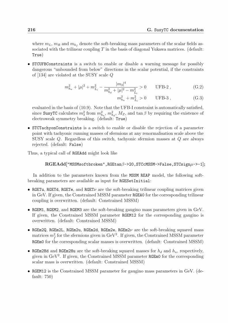
216 G. SusyTC documentation
where mL, mR and mhf denote the soft-breaking mass parameters of the scalar fields as-sociated with the trilinear coupling T in the basis of diagonal Yukawa matrices. (default:True)
• STCUFBConstraints is a switch to enable or disable a warning message for possiblydangerous “unbounded from below” directions in the scalar potential, if the constraintsof [134] are violated at the SUSY scale Q
m2hu + |µ|2 +m2
Li− |m3|4m2hd
+ |µ|2 −m2Li
> 0 UFB-2 , (G.2)
m2hu +m2
Li> 0 UFB-3 , (G.3)
evaluated in the basis of (10.9). Note that the UFB-I constraint is automatically satisfied,since SusyTC calculates m2
3 from m2hu
, m2hd
, MZ , and tan β by requiring the existence ofelectroweak symmetry breaking. (default: True)
• STCTachyonConstraints is a switch to enable or disable the rejection of a parameterpoint with tachyonic running masses of sfermions at any renormalisation scale above theSUSY scale Q. Regardless of this switch, tachyonic sfermion masses at Q are alwaysrejected. (default: False)
Thus, a typical call of RGEAdd might look like
RGEAdd["MSSMsoftbroken",RGEtanβ->20,STCcMSSM->False,STCsignµ->-1];
In addition to the parameters known from the MSSM REAP model, the following soft-breaking parameters are available as input for RGESetInitial:
• RGETu, RGETd, RGETe, and RGETν are the soft-breaking trilinear coupling matrices givenin GeV. If given, the Constrained MSSM parameter RGEA0 for the corresponding trilinearcoupling is overwritten. (default: Constrained MSSM)
• RGEM1, RGEM2, and RGEM3 are the soft-breaking gaugino mass parameters given in GeV.If given, the Constrained MSSM parameter RGEM12 for the corresponding gaugino isoverwritten. (default: Constrained MSSM)
• RGEm2Q, RGEm2L, RGEm2u, RGEm2d, RGEm2e, RGEm2ν are the soft-breaking squared massmatrices m2
ffor the sfermions given in GeV2. If given, the Constrained MSSM parameter
RGEm0 for the corresponding scalar masses is overwritten. (default: Constrained MSSM)
• RGEm2Hd and RGEm2Hu are the soft-breaking squared masses for hd and hu, respectively,given in GeV2. If given, the Constrained MSSM parameter RGEm0 for the correspondingscalar mass is overwritten. (default: Constrained MSSM)
• RGEM12 is the Constrained MSSM parameter for gaugino mass parameters in GeV. (de-fault: 750)

217
• RGEm0 is the Constrained MSSM parameter for all soft-breaking masses of scalars inGeV. (default: 1500)
• RGEA0 is the Constrained MSSM parameter A0 for trilinear couplings, e.g. Tf = A0Yf ,in GeV. (default: -500)
An example for an input at a GUT scale of 2 · 1016 GeV would be
RGESetInitial[2·10^16,RGEM1->863,RGEM2->131,RGEM3->-392,RGESuggestion->"GUT"];
The solution at a lower energy scale such as MZ ≈ 91 GeV can now be obtained by theREAP command RGESolve:
RGESolve[91.19,2·10^16];
Some parameter points might lead to tachyonic sparticle masses. In such instances theevaluation of SusyTC is stopped and an error message is returned using the Mathematicacommand Throw. In order to properly catch such error messages, we therefore recommendto use instead
Catch[RGESolve[91.19,2·10^16],TachyonicMass];
In addition to the parameters known from the MSSM REAP model, the following soft-breaking parameters are available for RGEGetSolution at all energy scales between MGUT
and the SUSY scale Q:
• RGETu, RGETd, RGETe, and RGETν are used to get the soft-breaking trilinear couplingmatrices.
• RawTν is used to get the raw (internal representation) of the soft-breaking trilinear matrixfor sneutrinos.
• RGEM1, RGEM2, and RGEM3 are used to get the soft-breaking gaugino mass parameters.
• RGEm2Q, RGEm2L, RGEm2u, RGEm2d, RGEm2e, RGEm2ν are used to get the soft-breakingsquared mass matrices m2
ffor the sfermions.
• RGEm2Hd and RGEm2Hu are used to get the soft-breaking squared masses for hd and hu,respectively.
To obtain the running DR gluino mass at a scale of two TeV for example, one uses
RGEGetSolution[2000,RGEM3];

218 G. SusyTC documentation
With SusyTC the DR sparticle spectrum is automatically calculated. The followingfunctions are included in SusyTC:
• STCGetSUSYScale[] returns the SUSY scale Q in GeV.
• STCGetSUSYSpectrum[] returns a list of replacement rules for the SUSY scale Q, theDR tree-level values of µ and m3, and the DR sparticle masses in GeV and (tree-level)mixing matrices at the SUSY scale. In detail it contains
– "Q" the SUSY scale Q.
– "µ","m3" the values of µ and m3.
– "M1","M2","M3" are the gaugino mass parameters.
– "Mh","MH","MA","MHp" the (tree-level) masses of the MSSM Higgs bosons.1
– "mχ0" a list of the four neutralino masses.
– "mχp" a list of the two chargino masses.
– "msude" a 3×6 array of the six up-type quarks, down-type squarks and charged sleptonmasses, respectively.
– "msν" a list of the three light sneutrino masses.
– "θW" the weak mixing angle.
– "tanα" the mixing angle of the CP-even Higgs bosons.
– "N" the mixing matrix of neutralinos.
– "U","V" the mixing matrices for charginos.
– "Wude" a list of the three sparticle mixing matrices for up-type squarks, down-typesquarks and charged sleptons.
– "Wν" the mixing matrix of the three light sneutrinos.
To obtain for example the SUSY scale and the tree-level masses of the charginos call
"Q"/.STCGetSUSYSpectrum[];
"mχp"/.STCGetSUSYSpectrum[];
The squark masses and charged slepton masses are contained in a joint list as mu,md,me,and analogously for the sfermion mixing matrices. To obtain for example the up-typesquark masses, the charged slepton mixing matrix, and the sneutrino masses type
("msude"/.STCGetSUSYSpectrum[])[[1]];
("Wude"/.STCGetSUSYSpectrum[])[[3]];
"msν"/.STCGetSUSYSpectrum[];
• STCGetOneLoopValues[] returns a list of replacement rules containing
1Note that there is no CP-violation in the MSSM Higgs sector on tree-level.

219
– "µ","m3" the one-loop corrected DR µ-parameter and m3 as in (10.15) and (10.16)at the SUSY scale Q in GeV.
– "vev" the one-loop DR vev v as in (10.20) at the SUSY scale Q in GeV.
– "MHp" ("MA") the pole-mass mH+ (mA) of the charged (CP-odd) Higgs boson forSTCcMSSM = True (False) in GeV.
The value of µ can for example be obtained from
"µ"/.STCGetOneLoopValues[];
• STCGetSCKMValues[] returns a list of replacement rules with the soft-breaking masssquared and trilinear coupling matrices in the SCKM basis, where sparticles are rotatedanalogously with their corresponding superpartners2. Since they are used for the self-energies calculation as described in the previous appendix F, they are returned in SLHA2convention [123]! In detail, there are
– "VCKM" the CKM mixing matrix.
– "VPMNS" the PMNS mixing matrix.
– SCKMBasis["m2Q"], SCKMBasis["m2u"], SCKMBasis["m2d"] the squark soft-breakingmass squared matrices in the Super-CKM basis with SLHA2 convetions in GeV2.
– SCKMBasis["m2L"], SCKMBasis["m2e"] the slepton soft-breaking mass squared ma-trices in the Super-PMNS basis with SLHA2 conventions in GeV2.
– SCKMBasis["T"] a list of the three trilinear coupling matrices for up-type squarks,down-type squarks, and charged sleptons in the SCKM basis with SLHA2 conventionsin GeV.
– SCKMBasis["Y"] a 3×3 array of the Yukawa coupling singular values for up-typesquarks, down-type squarks, and charged sleptons.
To obtain the down-type trilinear coupling matrix and the mass squared matrix of thesquark doublet in the SLHA basis for example, type
(SCKMBasis["T"]/.STCGetSCKMValues[])[[2]];
SCKMBasis["m2Q"]/.STCGetSCKMValues[];
• STCGetInternalValues[] returns everything that is internally used for the calculationof the threshold corrections and sparticle spectrum, i.e. the results from STCGetSCKMValues[]
and STCGetSUSYSpectrum[] with the one-loop corrected parameters from STCGetOneLoopValues[]
replacing tree-level ones if available. We recommend to the user to use those separatefunctions instead.
As additional feature, SusyTC optionally supports input and output as SLHA “LesHouches” files. These files follow SLHA conventions [123,194]:
2Here we use the term “SCKM” for the Super-CKM and Super-PMNS basis.

220 G. SusyTC documentation
• STCSLHA2Input[“Path”] loads an “Les Houches” input file stored in “Path” and exe-cutes REAP and SusyTC. If no path is given, the default path is assumed as “SusyTC.in”in the Mathematica notebook directory. An important difference to other spectrum cal-culators is the pure “top-down” approach by SusyTC, i.e. there is no attempt of fittingSM inputs at a low scale or calculating a GUT scale from gauge couplings unification.Instead, all input is given at a user-defined high energy scale, which is then evolved tolower scales. The input should be given in the flavour basis in SLHA 2 convention [123]as in (5.64) and (5.65), and the seesaw parameters in the convention (5.77). The relationbetween the SusyTC conventions of chapter 10 and the SLHA 2 conventions is given in10.2. In the following, we list all SLHA 2 input blocks, which are available in SusyTC:
– Block MODSEL: The only available switch is:5 : (Default = 2) CP violation (STCcMSSM)
– Block SusyTCInput: Switches (1=True, 0=False) are defined for RGEAdd:1 : (Default = 1) STCSusyScaleFromStops2 : (Default = 1) STCSearchSMTransition3 : (Default = 1) STCCCBConstraints4 : (Default = 1) STCUFBConstraints5 : (Default = 1) Print a Warning in case of Tachyonic masses6 : (Default = 1) One or Two Loop RGEs
– Block MINPAR: Constrained MSSM parameters as defined in [123,194]. Note however,that the input value of tan β is interpreted to be given at the SUSY scale.
– Block IMMINPAR: Reads the sinφµ in case of the complex MSSM:4 : sinφµ
– Block EXTPAR:0 : (Default = 2 · 1016): Minput Input scale in GeVNote that with SusyTC an automatic calculation of the GUT scale is not possible.The remainder of the block works as usual, e.g. optionally one can overwrite commonConstrained MSSM gaugino or Higgs soft-breaking parameters:1 : M1(Minput) bino mass (real part) in GeV2 : M2(Minput) wino mass (real part) in GeV3 : M3(Minput) gluino mass (real part) in GeV21 : m2
hd(Minput) in GeV2
22 : m2hu
(Minput) in GeV2
Imaginary components for the gaugino masses can be given in Block IMEXTPAR.
– Block IMEXTPAR: as defined in [123].
– Block QEXTPAR: low energy input:0 : (Default = 91.1876): The low energy scale in GeV to which REAP evolves the SMRGEs.23 : “SUSY scale” Q, where the MSSM is matched to the SM. If this entry is set, itoverwrites the automatically calculated SUSY scale.
221
– Block GAUGE: the DR gauge couplings at the input scale1 : g1(Minput) U(1) gauge coupling2 : g2(Minput) SU(2) gauge coupling3 : g3(Minput) SU(3) gauge coupling
– Block YU, Block YD, Block YE, Block YN: The real parts of the Yukawa matricesYu, Yd, Ye, and Yν in the flavour basis (5.64) and (5.77). They should be given in theFORTRAN format (1x,I2,1x,I2,3x,1P,E16.8,0P,3x,‘#’,1x,A), where the first twointegers correspond to the indices and the double precision number to Re(Yij).
– Block IMYU, Block IMYD, Block IMYE, Block IMYN: The imaginary parts of theYukawa matrices Yu, Yd, Ye, and Yν in the flavour basis (5.64) and (5.77). They aregiven in the same format as the real parts.
– Block MN: The real part of the symmetric Majorana mass matrix Mn of the right-handed neutrinos in the flavour basis (5.77) in GeV. Only the “upper-triangle” entriesshould be given, the input format is as for the Yukawa matrices.
– Block IMMN: The imaginary part of the symmetric Majorana mass matrix Mn of theright-handed neutrinos in the flavour basis (5.77) in GeV. Only the “upper-triangle”entries should be given, the input format is as for the Yukawa matrices.
The remaining blocks can be given optionally to overwrite Constrained MSSM inputboundary conditions:
– Block TU, Block TD, Block TE, Block TN: The real parts of the trilinear soft-breaking matrices Tu, Td, Te, and Tν in GeV in the flavour basis (5.65). They shouldbe given in the same format as the Yukawa matrices.
– Block IMTU, Block IMTD, Block IMTE, Block IMTN: The imaginary parts of thetrilinear soft-breaking matrices Tu, Td, Te, and Tν in GeV in the flavour basis (5.65).They should be given in the same format as the Yukawa matrices.
– Block MSQ2, Block MSU2, Block MSD2, Block MSL2, Block MSE2,
Block MSN2: The real parts of the soft-breaking mass squared matrices m2Q
, m2u, m
2d,
m2L, m2
e, and m2ν in GeV2 in the flavour basis (5.65). Only the “upper-triangle” entries
should be given, the input format is as for the Yukawa matrices.
– Block IMMSQ2, Block IMMSU2, Block IMMSD2,Block IMMSL2,
Block IMMSE2, Block IMMSN2: The imaginary parts of the soft-breaking mass squaredmatrices m2
Q, m2
u, m2d, m2
L, m2
e, and m2ν in GeV2 in the flavour basis (5.65). Only the
“upper-triangle” entries should be given, the input format is as for the Yukawa ma-trices.
• STCWriteSLHA2Output[“Path”] writes a “Les Houches” [123,194] output file to “Path”.If no path is given, the output is saved in the Mathematica notebook directory as“SusyTC.out”. The output follows SLHA conventions, with the following exceptions:

222 G. SusyTC documentation
– Block MASS: The mass spectrum is given as DR masses in GeV at the SUSY scale.The only exception is the pole mass MH+ (MA) for CP violation turned on (off).
– Block ALPHA: the tree-level Higgs mixing angle αtree.
– Block HMIX: Instead of MA we give101 : m3
The other blocks follow the SLHA2 output conventions, e.g. DR values at the SUSY scalein the Super-CKM/Super-PMNS basis. To avoid confusion, the blocks Block DSQMIX,
Block USQMIX, Block SELMIX, Block SNUMIX and the corresponding blocks for theimaginary entries, return the sfermion mixing matrices Rf in SLHA 2 convention!

Bibliography
[1] S. Antusch, C. Gross, V. Maurer, and C. Sluka, θPMNS13 = θC /
√2 from
GUTs, Nucl. Phys. B866, 255 (2013), arXiv: 1205.1051.
[2] S. Antusch, C. Gross, V. Maurer, and C. Sluka, A flavour GUT model withθPMNS
13 ' θC /√
2, Nucl. Phys. B877, 772 (2013), arXiv: 1305.6612.
[3] S. Antusch, C. Gross, V. Maurer, and C. Sluka, Inverse neutrino masshierarchy in a flavour GUT model, Nucl. Phys. B879, 19 (2014), arXiv: 1306.3984.
[4] S. Antusch, I. de Medeiros Varzielas, V. Maurer, C. Sluka, and M. Spin-rath, Towards predictive flavour models in SUSY SU(5) GUTs with doublet-tripletsplitting, JHEP 1409, 141 (2014), arXiv: 1405.6962.
[5] S. Antusch and C. Sluka, Predicting the Sparticle Spectrum from GUTs via SUSYThreshold Corrections with SusyTC, (2015), arXiv: 1512.06727.
[6] S. L. Glashow, Partial Symmetries of Weak Interactions, Nucl. Phys. 22, 579(1961).
S. Weinberg, A Model of Leptons, Phys. Rev. Lett. 19, 1264 (1967).
A. Salam, Weak and Electromagnetic Interactions, Conf. Proc. C680519, 367(1968), reprinted in A. Ali et al. [editors], Selected papers of Abdus Salam: withcommentary, World scientific series in 20th century physics 5, 244 (1994).
S. L. Glashow, J. Iliopoulos, and L. Maiani, Weak Interactions with Lepton-Hadron Symmetry, Phys. Rev. D2, 1285 (1970).
[7] D. J. Gross and F. Wilczek, Ultraviolet Behavior of Nonabelian Gauge Theories,Phys. Rev. Lett. 30, 1343 (1973).
S. Weinberg, Nonabelian Gauge Theories of the Strong Interactions, Phys. Rev.Lett. 31, 494 (1973).
H. Fritzsch, M. Gell-Mann, and H. Leutwyler, Advantages of the ColorOctet Gluon Picture, Phys. Lett. B47, 365 (1973).
[8] D. J. Gross and F. Wilczek, Asymptotically Free Gauge Theories. 1, Phys. Rev.D8, 3633 (1973).
224 BIBLIOGRAPHY
D. J. Gross and F. Wilczek, Asymptotically Free Gauge Theories. 2, Phys. Rev.D9, 980 (1974).
H. D. Politzer, Reliable Perturbative Results for Strong Interactions?, Phys. Rev.Lett. 30, 1346 (1973).
H. D. Politzer, Asymptotic Freedom: An Approach to Strong Interactions, Phys.Rept. 14, 129 (1974).
[9] G. ’t Hooft, Renormalization of Massless Yang-Mills Fields, Nucl. Phys. B33,173 (1971).
G. ’t Hooft, Renormalizable Lagrangians for Massive Yang-Mills Fields, Nucl.Phys. B35, 167 (1971).
[10] F. Englert and R. Brout, Broken Symmetry and the Mass of Gauge VectorMesons, Phys. Rev. Lett. 13, 321 (1964).
[11] P. W. Higgs, Broken symmetries, massless particles and gauge fields, Phys. Lett.12, 132 (1964).
P. W. Higgs, Broken Symmetries and the Masses of Gauge Bosons, Phys. Rev.Lett. 13, 508 (1964).
P. W. Higgs, Spontaneous Symmetry Breakdown without Massless Bosons, Phys.Rev. 145, 1156 (1966).
[12] H. K. Dreiner, H. E. Haber, and S. P. Martin, Two-component spinor tech-niques and Feynman rules for quantum field theory and supersymmetry, Physics Re-ports 494, 1 (2010), arXiv: 0812.1594 [hep-ph].
[13] E. C. G. Stueckelberg, Interaction energy in electrodynamics and in the fieldtheory of nuclear forces (Part I), Helv. Phys. Acta 11, 225 (1938), [in German],reprinted in J. Lacki, H. Ruegg and G. Wanders [Editors], E.C.G. Stueck-elberg, An Unconventional Figure of Twentieth Century Physisc: Selected ScientificPapers with Commentaries, Birkhauser Verlag, Basel, 251 (2009).
E. C. G. Stueckelberg, Interaction energy in electrodynamics and in the field the-ory of nuclear forces (Part II and III), Helv. Phys. Acta 11, 299 (1938), [in German],reprinted in J. Lacki, H. Ruegg and G. Wanders [Editors], E.C.G. Stueck-elberg, An Unconventional Figure of Twentieth Century Physisc: Selected ScientificPapers with Commentaries, Birkhauser Verlag, Basel, 273 (2009).
[14] K. A. Olive et al., Review of Particle Physics, Chin. Phys. C38, 090001 (2014).
[15] N. Cabibbo, Unitary Symmetry and Leptonic Decays, Phys. Rev. Lett. 10, 531(1963).
[16] M. Kobayashi and T. Maskawa, CP Violation in the Renormalizable Theory ofWeak Interaction, Prog. Theor. Phys. 49, 652 (1973).

BIBLIOGRAPHY 225
[17] S. F. King, Constructing the large mixing angle MNS matrix in seesaw models withright-handed neutrino dominance, JHEP 0209, 011 (2002), arXiv: hep-ph/0204360.
[18] P. J. Mohr, B. N. Taylor, and D. B. Newell, CODATA Recommended Valuesof the Fundamental Physical Constants: 2010, Rev. Mod. Phys. 84, 1527 (2012),arXiv: 1203.5425 [atom-ph].
[19] K. G. Wilson, Confinement of Quarks, Phys. Rev. D10, 2445 (1974).
[20] S. Weinberg, Phenomenological Lagrangians, Physica A96, 327 (1979).
[21] J. Gasser and H. Leutwyler, Chiral Perturbation Theory to One Loop, AnnalsPhys. 158, 142 (1984).
[22] H. Leutwyler, The Ratios of the light quark masses, Phys.Lett. B378, 313 (1996),arXiv: hep-ph/9602366.
[23] N. Isgur and M. B. Wise, Weak Decays of Heavy Mesons in the Static QuarkApproximation, Phys. Lett. B232, 113 (1989).
[24] S. L. Adler, Axial vector vertex in spinor electrodynamics, Phys. Rev. 177, 2426(1969).
[25] J. S. Bell and R. Jackiw, A PCAC puzzle: pi0 → gamma gamma in the sigmamodel, Nuovo Cim. A60, 47 (1969).
[26] D. J. Gross and R. Jackiw, Effect of anomalies on quasirenormalizable theories,Phys. Rev. D6, 477 (1972).
[27] G. ’t Hooft, Naturalness, chiral symmetry, and spontaneous chiral symmetrybreaking, NATO Sci. Ser. B 59, 135 (1980).
[28] G. ’t Hooft, Symmetry Breaking Through Bell-Jackiw Anomalies, Phys. Rev. Lett.37, 8 (1976).
G. ’t Hooft, Computation of the Quantum Effects Due to a Four-DimensionalPseudoparticle, Phys. Rev. D14, 3432 (1976), [Erratum: Phys. Rev. D18, 2199(1978)].
[29] R. Jackiw and C. Rebbi, Vacuum Periodicity in a Yang-Mills Quantum Theory,Phys. Rev. Lett. 37, 172 (1976).
[30] R. D. Peccei and H. R. Quinn, CP Conservation in the Presence of Instantons,Phys. Rev. Lett. 38, 1440 (1977).
[31] S. Weinberg, A New Light Boson?, Phys. Rev. Lett. 40, 223 (1978).
F. Wilczek, Problem of Strong p and t Invariance in the Presence of Instantons,Phys. Rev. Lett. 40, 279 (1978).

226 BIBLIOGRAPHY
[32] S. Antusch, M. Holthausen, M. A. Schmidt, and M. Spinrath, Solving theStrong CP Problem with Discrete Symmetries and the Right Unitarity Triangle, Nucl.Phys. B877, 752 (2013), arXiv: 1307.0710 [hep-ph].
[33] A. Bosma, 21-cm line studies of spiral galaxies. 2. The distribution and kinematicsof neutral hydrogen in spiral galaxies of various morphological types., Astron. J. 86,1825 (1981).
[34] G. F. Smoot et al., Structure in the COBE differential microwave radiometer firstyear maps, Astrophys. J. 396, L1 (1992).
C. L. Bennett et al., Nine-Year Wilkinson Microwave Anisotropy Probe (WMAP)Observations: Final Maps and Results, Astrophys. J. Suppl. 208, 20 (2013), arXiv:1212.5225 [astro-ph.CO].
[35] P. A. R. Ade et al., Planck 2015 results. XIII. Cosmological parameters, (2015),arXiv: 1502.01589 [astro-ph.CO].
[36] M. Markevitch, A. H. Gonzalez, D. Clowe, A. Vikhlinin, L. David,W. Forman, C. Jones, S. Murray, and W. Tucker, Direct constraints on thedark matter self-interaction cross-section from the merging galaxy cluster 1E0657-56,Astrophys. J. 606, 819 (2004), arXiv: astro-ph/0.09303.
D. Clowe, A. Gonzalez, and M. Markevitch, Weak lensing mass reconstruc-tion of the interacting cluster 1E0657-558: Direct evidence for the existence of darkmatter, Astrophys. J. 604, 596 (2004), arXiv: astro-ph/0312273.
[37] C. Alcock et al., The MACHO project lmc variable star inventory. ix. frequencyanalysis of the first overtone rr lyrae stars and the indication for nonradial pulsations,Astrophys. J. 542, 257 (2000), arXiv: astro-ph/0005361.
P. Tisserand et al., Limits on the Macho Content of the Galactic Halo from theEROS-2 Survey of the Magellanic Clouds, Astron. Astrophys. 469, 387 (2007), arXiv:astro-ph/0607207.
L. Wyrzykowski et al., The OGLE View of Microlensing towards the MagellanicClouds. IV. OGLE-III SMC Data and Final Conclusions on MACHOs, Mon. Not.Roy. Astron. Soc. 416, 2949 (2011), arXiv: 1106.2925 [astro-ph.GA].
[38] B. W. Lee and S. Weinberg, Cosmological Lower Bound on Heavy NeutrinoMasses, Phys. Rev. Lett. 39, 165 (1977).
P. Hut, Limits on Masses and Number of Neutral Weakly Interacting Particles,Phys. Lett. B69, 85 (1977).
M. I. Vysotsky, A. D. Dolgov, and Y. B. Zeldovich, Cosmological Restrictionon Neutral Lepton Masses, JETP Lett. 26, 188 (1977), [Pisma Zh. Eksp. Teor. Fiz.26, 200 (1977)].
BIBLIOGRAPHY 227
J. E. Gunn, B. W. Lee, I. Lerche, D. N. Schramm, and G. Steigman,Some Astrophysical Consequences of the Existence of a Heavy Stable Neutral Lepton,Astrophys. J. 223, 1015 (1978).
G. Steigman, C. L. Sarazin, H. Quintana, and J. Faulkner, Dynamicalinteractions and astrophysical effects of stable heavy neutrinos, Astron. J. 83, 1050(1978).
[39] M. S. Turner, Windows on the Axion, Phys. Rept. 197, 67 (1990).
G. G. Raffelt, Astrophysical methods to constrain axions and other novel particlephenomena, Phys. Rept. 198, 1 (1990).
[40] J. R. Ellis, J. S. Hagelin, D. V. Nanopoulos, K. A. Olive, and M. Sred-nicki, Supersymmetric Relics from the Big Bang, Nucl. Phys. B238, 453 (1984).
[41] A. G. Riess et al., Observational evidence from supernovae for an acceleratinguniverse and a cosmological constant, Astron. J. 116, 1009 (1998), arXiv: astro-ph/9805201.
S. Perlmutter et al., Measurements of Omega and Lambda from 42 high redshiftsupernovae, Astrophys. J. 517, 565 (1999), arXiv: astro-ph/9812133.
P. A. R. Ade et al., Planck 2015 results. XIV. Dark energy and modified gravity,(2015), arXiv: 1502.01590 [astro-ph.CO].
[42] B. Pontecorvo, Mesonium and anti-mesonium, Sov. Phys. JETP 6, 429 (1957),[Zh. Eksp. Teor. Fiz.33,549(1957)].
B. Pontecorvo, Inverse beta processes and nonconservation of lepton charge, Sov.Phys. JETP 7, 172 (1958), [Zh. Eksp. Teor. Fiz.34,247(1957)].
B. Pontecorvo, Neutrino Experiments and the Problem of Conservation of Lep-tonic Charge, Sov. Phys. JETP 26, 984 (1968), [Zh. Eksp. Teor. Fiz.53,1717(1967)].
[43] V. N. Gribov and B. Pontecorvo, Neutrino astronomy and lepton charge, Phys.Lett. B28, 493 (1969).
[44] R. Davis, Solar neutrinos. II: Experimental, Phys. Rev. Lett. 12, 303 (1964).
R. Davis, Jr., D. S. Harmer, and K. C. Hoffman, Search for neutrinos fromthe sun, Phys. Rev. Lett. 20, 1205 (1968).
[45] B. T. Cleveland, T. Daily, R. Davis, Jr., J. R. Distel, K. Lande, C. K.Lee, P. S. Wildenhain, and J. Ullman, Measurement of the solar electronneutrino flux with the Homestake chlorine detector, Astrophys. J. 496, 505 (1998).
W. Hampel et al., GALLEX solar neutrino observations: Results for GALLEX IV,Phys. Lett. B447, 127 (1999).

228 BIBLIOGRAPHY
Q. R. Ahmad et al., Direct evidence for neutrino flavor transformation from neu-tral current interactions in the Sudbury Neutrino Observatory, Phys. Rev. Lett. 89,011301 (2002), arXiv: nucl-ex/0204008.
S. Fukuda et al., Determination of solar neutrino oscillation parameters using1496 days of Super-Kamiokande I data, Phys. Lett. B539, 179 (2002), arXiv: hep-ex/0205075.
Y. Ashie et al., Evidence for an oscillatory signature in atmospheric neutrinooscillation, Phys. Rev. Lett. 93, 101801 (2004), arXiv: hep-ex/0404034.
T. Araki et al., Measurement of neutrino oscillation with KamLAND: Evidence ofspectral distortion, Phys. Rev. Lett. 94, 081801 (2005), arXiv: hep-ex/0406035.
M. Altmann et al., Complete results for five years of GNO solar neutrino observa-tions, Phys. Lett. B616, 174 (2005), arXiv: hep-ex/0504037.
J. N. Abdurashitov et al., Measurement of the solar neutrino capture rate withgallium metal. III: Results for the 2002–2007 data-taking period, Phys. Rev. C80,015807 (2009), arXiv: 0901.2200 [nucl-ex].
P. Adamson et al., Measurement of the neutrino mass splitting and flavor mixingby MINOS, Phys. Rev. Lett. 106, 181801 (2011), arXiv: 1103.0340 [hep-ex].
[46] K. Abe et al. [T2K Collaboration], Indication of Electron Neutrino Appearancefrom an Accelerator-produced Off-axis Muon Neutrino Beam, Phys.Rev.Lett. 107,041801 (2011), arXiv: 1106.2822 [hep-ex].
Y. Abe et al. [DOUBLE-CHOOZ Collaboration], Indication for the disappear-ance of reactor electron antineutrinos in the Double Chooz experiment, Phys.Rev.Lett.108, 131801 (2012), arXiv: 1112.6353 [hep-ex].
F. P. An et al. [DAYA-BAY Collaboration], Observation of electron-antineutrino disappearance at Daya Bay, Phys.Rev.Lett. 108, 171803 (2012), arXiv:1203.1669 [hep-ex].
J. K. Ahn et al. [RENO Collaboration], Observation of Reactor ElectronAntineutrino Disappearance in the RENO Experiment, Phys.Rev.Lett. 108, 191802(2012), arXiv: 1204.0626 [hep-ex].
[47] A. Strumia and F. Vissani, Neutrino masses and mixings and..., (2006), arXiv:hep-ph/0606054.
[48] J. Lesgourgues, G. Mangano, G. Miele, and S. Pastor, Neutrino Cosmology,Cambridge University Press, New York, 2013.
[49] S. F. King and C. Luhn, Neutrino Mass and Mixing with Discrete Symmetry,Rept. Prog. Phys. 76, 056201 (2013), arxXiv: 1301.1340 [hep-ph].
[50] V. N. Aseev et al., An upper limit on electron antineutrino mass from Troitskexperiment, Phys. Rev. D84, 112003 (2011).

BIBLIOGRAPHY 229
[51] S. Weinberg, Baryon and Lepton Nonconserving Processes, Phys. Rev. Lett. 43,1566 (1979).
S. Weinberg, Varieties of Baryon and Lepton Nonconservation, Phys. Rev. D22,1694 (1980).
[52] P. Minkowski, µ → eγ at a Rate of One Out of 109 Muon Decays?, Phys. Lett.B67, 421 (1977).
M. Gell-Mann, P. Ramond, and R. Slansky, Complex Spinors and UnifiedTheories, Conf. Proc. C790927, 315 (1979), in P. Van Nieuwenhuizen and D. Z.Freedman [Editors], Supergravity: Proceedings of the Supergravity Workshop atStony Brook, 27-29 September 1979, New York, 315 (1979), arXiv: 1306.4669 [hep-th].
T. Yanagida, Horizontal symmetry and masses of neutrinos, Conf. Proc.C7902131, 95 (1979), in O. Sawada and A. Sugamoto [Editors], Proceed-ings: Workshop on the Unified Theories and the Baryon Number in the Universe,Tsukuba, Japan, 13-14 Feb 1979, 95 (1979).
S. L. Glashow, The Future of Elementary Particle Physics, NATO Sci. Ser. B61, 687 (1980), in M. Levy et al. [Editors], Quarks and Leptons: Cargese 1979,Springer US, 687 (1980).
R. N. Mohapatra and G. Senjanovic, Neutrino Mass and Spontaneous ParityViolation, Phys. Rev. Lett. 44, 912 (1980).
J. Schechter and J. W. F. Valle, Neutrino Masses in SU(2) x U(1) Theories,Phys. Rev. D22, 2227 (1980).
[53] G. B. Gelmini and M. Roncadelli, Left-Handed Neutrino Mass Scale and Spon-taneously Broken Lepton Number, Phys. Lett. B99, 411 (1981).
[54] R. Foot, H. Lew, X. G. He, and G. C. Joshi, Seesaw Neutrino Masses Inducedby a Triplet of Leptons, Z. Phys. C44, 441 (1989).
[55] R. N. Mohapatra and J. W. F. Valle, Neutrino Mass and Baryon NumberNonconservation in Superstring Models, Phys. Rev. D34, 1642 (1986).
[56] T. P. Cheng and L.-F. Li, On Weak Interaction Induced Neutrino Oscillations,Phys. Rev. D17, 2375 (1978).
A. Zee, A Theory of Lepton Number Violation, Neutrino Majorana Mass, andOscillation, Phys. Lett. B93, 389 (1980), [Erratum: Phys. Lett.B95,461(1980)].
T. P. Cheng and L.-F. Li, Neutrino Masses, Mixings and Oscillations in SU(2) xU(1) Models of Electroweak Interactions, Phys. Rev. D22, 2860 (1980).
[57] Y. Katayama, K. Matumoto, S. Tanaka, and E. Yamada, Possible unifiedmodels of elementary particles with two neutrinos, Prog. Theor. Phys. 28, 675 (1962).

230 BIBLIOGRAPHY
Z. Maki, M. Nakagawa, and S. Sakata, Remarks on the unified model of ele-mentary particles, Prog. Theor. Phys. 28, 870 (1962).
M. Nakagawa, H. Okonogi, S. Sakata, and A. Toyoda, Possible existence ofa neutrino with mass and partial conservation of muon charge, Prog. Theor. Phys.30, 727 (1963).
[58] S. P. Mikheev and A. Yu. Smirnov, Resonance Amplification of Oscillationsin Matter and Spectroscopy of Solar Neutrinos, Sov. J. Nucl. Phys. 42, 913 (1985),[Yad. Fiz.42,1441(1985)].
S. P. Mikheev and A. Yu. Smirnov, Resonant amplification of neutrino oscilla-tions in matter and solar neutrino spectroscopy, Nuovo Cim. C9, 17 (1986).
L. Wolfenstein, Neutrino Oscillations in Matter, Phys. Rev. D17, 2369 (1978).
[59] S. Nussinov, Solar Neutrinos and Neutrino Mixing, Phys. Lett. B63, 201 (1976).
B. Kayser, On the Quantum Mechanics of Neutrino Oscillation, Phys. Rev. D24,110 (1981).
C. Giunti, C. W. Kim, and U. W. Lee, When do neutrinos really oscillate?:Quantum mechanics of neutrino oscillations, Phys. Rev. D44, 3635 (1991).
J. Rich, The Quantum mechanics of neutrino oscillations, Phys. Rev. D48, 4318(1993).
W. Grimus, P. Stockinger, and S. Mohanty, The Field theoretical approachto coherence in neutrino oscillations, Phys. Rev. D59, 013011 (1999), arXiv: hep-ph/9807442.
[60] L. Stodolsky, The Unnecessary wave packet, Phys. Rev. D58, 036006 (1998),arXiv: hep-ph/9802387.
[61] S. M. Bilenky and S. T. Petcov, Massive Neutrinos and Neutrino Oscillations,Rev. Mod. Phys. 59, 671 (1987), [Erratum: Rev. Mod. Phys. 60, 575 (1988)].
[62] M. C. Gonzalez-Garcia, M. Maltoni, and T. Schwetz, Global Analyses ofNeutrino Oscillation Experiments, (2015), arXiv: 1512.06856 [hep-ph].
[63] V. D. Barger, S. Pakvasa, T. J. Weiler, and K. Whisnant, Bimaximalmixing of three neutrinos, Phys. Lett. B437, 107 (1998), arXiv: hep-ph/9806387.
[64] P. F. Harrison, D. H. Perkins, and W. G. Scott, Tri-bimaximal mixing andthe neutrino oscillation data, Phys. Lett. B530, 167 (2002), arXiv: hep-ph/0202074.
[65] S. Antusch and S. F. King, Charged lepton corrections to neutrino mixing anglesand CP phases revisited, Phys.Lett. B631, 42 (2005), arXiv: hep-ph/0508044.
[66] S. F. King, Predicting neutrino parameters from SO(3) family symmetry and quark-lepton unification, JHEP 0508, 105 (2005), arXiv: hep-ph/0506297.
BIBLIOGRAPHY 231
[67] I. Masina, A Maximal atmospheric mixing from a maximal CP violating phase,Phys. Lett. B633, 134 (2006), arXiv: hep-ph/0508031.
S. Antusch, P. Huber, S. F. King, and T. Schwetz, Neutrino mixing sumrules and oscillation experiments, JHEP 0704, 060 (2007), arXiv: hep-ph/0702286.
[68] C. Jarlskog, A Basis Independent Formulation of the Connection Between QuarkMass Matrices, CP Violation and Experiment, Z. Phys. C29, 491 (1985).
[69] M. Bishai, E. McCluskey, A. Rubbia, and M. Thomson, Long-Baseline Neutrino Facility (LBNF) and Deep Underground Neutrino Experiment(DUNE) Conceptual Design Report, Volume 1: The LBNF and DUNE Projects,(2015), LBNE-doc-10687-v9, http://http://lbne2-docdb.fnal.gov/cgi-bin/
RetrieveFile?docid=10687.
[70] G. Racah, On the symmetry of particle and antiparticle, Nuovo Cim. 14, 322(1937).
W. H. Furry, On transition probabilities in double beta-disintegration, Phys. Rev.56, 1184 (1939).
[71] J. Schechter and J. W. F. Valle, Neutrinoless Double beta Decay in SU(2) ×U(1) Theories, Phys. Rev. D25, 2951 (1982).
[72] A. S. Barabash, Double beta decay experiments: present status and prospects forthe future, Phys. Procedia 74, 416 (2015).
[73] S. F. King and C. Luhn, On the origin of neutrino flavour symmetry, JHEP 0910,093 (2009), arXiv: 0908.1897.
[74] S. F. King and N. N. Singh, Inverted hierarchy models of neutrino masses, Nucl.Phys. B596, 81 (2001), arXiv: hep-ph/0007243.
[75] C. D. Froggatt and H. B. Nielsen, Hierarchy of Quark Masses, Cabibbo Anglesand CP Violation, Nucl. Phys. B147, 277 (1979).
[76] E. Ma and G. Rajasekaran, Softly broken A(4) symmetry for nearly degenerateneutrino masses, Phys. Rev. D64, 113012 (2001), arXiv: hep-ph/0106291.
[77] K. S. Babu, E. Ma, and J. W. F. Valle, Underlying A(4) symmetry for theneutrino mass matrix and the quark mixing matrix, Phys. Lett. B552, 207 (2003),arXiv: hep-ph/0206292.
[78] G. Altarelli and F. Feruglio, Tri-bimaximal neutrino mixing from discretesymmetry in extra dimensions, Nucl. Phys. B720, 64 (2005), arXiv: hep-ph/0504165.
[79] H. Georgi and S. L. Glashow, Unity of All Elementary Particle Forces, Phys.Rev. Lett. 32, 438 (1974).
232 BIBLIOGRAPHY
[80] T. P. Cheng and L. F. Li, Gauge Theory of Elementary Particle Physics, OxfordUniversity Press, 536, 1984.
[81] G. Senjanovic, Course on grand unification, Springer Proc. Phys. 118, 137 (2008).
B. Bajc, Grand Unification and Proton Decay, (2011), lecture notes from the 2011ICTP Summer School on Particle Physics. http://users.ictp.it/ smr2244/Bajc.pdf.
[82] P. Nath and P. Fileviez Perez, Proton stability in grand unified theories, instrings and in branes, Phys. Rept. 441, 191 (2007).
[83] S. Antusch and M. Spinrath, New GUT predictions for quark and lepton massratios confronted with phenomenology, Phys. Rev. D79, 095004 (2009), arXiv:0902.4644 [hep-ph].
[84] R. Feger and T. W. Kephart, LieART - A Mathematica Application for Lie Al-gebras and Representation Theory, Comput. Phys. Commun. 192, 166 (2015), arXiv:1206.6379.
[85] R. Slansky, Group Theory for Unified Model Building, Phys. Rept. 79, 1 (1981).
[86] M. E. Machacek and M. T. Vaughn, Two Loop Renormalization Group Equa-tions in a General Quantum Field Theory. 1. Wave Function Renormalization, Nucl.Phys. B222, 83 (1983).
[87] H. Georgi and C. Jarlskog, A New Lepton - Quark Mass Relation In A UnifiedTheory, Phys.Lett. B86, 297 (1979).
[88] J. C. Pati and A. Salam, Unified Lepton-Hadron Symmetry and a Gauge Theoryof the Basic Interactions, Phys. Rev. D8, 1240 (1973).
[89] H. Georgi, The State of the Art – Gauge Theories, AIP Conf. Proc. 23, 575 (1975).
H. Fritzsch and P. Minkowski, Unified Interactions of Leptons and Hadrons,Annals Phys. 93, 193 (1975).
[90] S. M. Barr, A New Symmetry Breaking Pattern for SO(10) and Proton Decay,Phys. Lett. B112, 219 (1982).
[91] S. Antusch and V. Maurer, Running quark and lepton parameters at variousscales, JHEP 1311, 115 (2013), arXiv: 1306.6879.
[92] B. C. Allanach, S. F. King, G. K. Leontaris, and S. Lola, Yukawa texturesin string unified models with SU(4) x O(4) symmetry, Phys. Rev. D56, 2632 (1997),arXiv: hep-ph/9610517.
[93] S. Antusch, S. F. King, and M. Spinrath, GUT predictions for quark-leptonYukawa coupling ratios with messenger masses from non-singlets, Phys. Rev. D89,055027 (2014), arXiv: 1311.0877.

BIBLIOGRAPHY 233
[94] S. J. Gates, M. T. Grisaru, M. Rocek, and W. Siegel, Superspace Or OneThousand and One Lessons in Supersymmetry, Front. Phys. 58, 1 (1983), arXiv:hep-th/0108200.
[95] D. Bailin and A. Love, Supersymmetric Gauge Field Theory and String Theory,Taylor & Francis, 322, 1994.
[96] S. P. Martin, A Supersymmetry primer, Adv. Ser. Direct. High Energy Phys 18,1 (1998), arXiv: hep-ph/9709356.
[97] M. Drees, R. Godbole, and P. Roy, Theory and phenomenology of sparticles:An account of four-dimensional N=1 supersymmetry in high energy physics, WorldScientific Publishing, 555, 2004.
[98] D. J. H. Chung, L. L. Everett, G. L. Kane, S. F. King, J. D. Lykken, andL.-T. Wang, The Soft supersymmetry breaking Lagrangian: Theory and applica-tions, Phys. Rept. 407, 1 (2005), arXiv: hep-ph/0312378.
[99] M. Bertolini, Lectures on Supersymmetry, (2015), SISSA lecture notes,http://people.sissa.it/ bertmat/susycourse.pdf.
[100] J. Wess and B. Zumino, Supergauge Transformations in Four-Dimensions, Nucl.Phys. B70, 39 (1974).
[101] J. Wess and B. Zumino, Supergauge Invariant Extension of Quantum Electrody-namics, Nucl. Phys. B78, 1 (1974).
[102] A. Salam and J. A. Strathdee, Supergauge Transformations, Nucl. Phys. B76,477 (1974).
[103] P. Fayet and J. Iliopoulos, Spontaneously Broken Supergauge Symmetries andGoldstone Spinors, Phys. Lett. B51, 461 (1974).
P. Fayet, Higgs Model and Supersymmetry, Nuovo Cim. A31, 626 (1976).
[104] R. Delbourgo, Superfield Perturbation Theory and Renormalization, Nuovo Cim.A25, 646 (1975).
A. Salam and J. A. Strathdee, Feynman Rules for Superfields, Nucl. Phys. B86,142 (1975).
K. Fujikawa and W. Lang, Perturbation Calculations for the Scalar Multiplet ina Superfield Formulation, Nucl. Phys. B88, 61 (1975).
M. T. Grisaru, W. Siegel, and M. Rocek, Improved Methods for Supergraphs,Nucl. Phys. B159, 429 (1979).
[105] S. Antusch and M. Ratz, Supergraph techniques and two loop beta functions forrenormalizable and nonrenormalizable operators, JHEP 0207, 059 (2002), arXiv:hep-ph/0203027.

234 BIBLIOGRAPHY
[106] S. K. Soni and H. A. Weldon, Analysis of the Supersymmetry Breaking Inducedby N=1 Supergravity Theories, Phys. Lett. B126, 215 (1983).
[107] S. Antusch, S. F. King, and M. Malinsky, Third Family Corrections to Quarkand Lepton Mixing in SUSY Models with non-Abelian Family Symmetry, JHEP 0805,066 (2008), arXiv: 0712.3759.
[108] S. Antusch, S. F. King, and M. Malinsky, Third Family Corrections to Tri-bimaximal Lepton Mixing and a New Sum Rule, Phys. Lett. B671, 263 (2009), arXiv:0711.4727.
S. Antusch, S. F. King, and M. Malinsky, Perturbative Estimates of LeptonMixing Angles in Unified Models, Nucl. Phys. B820, 32 (2009), arXiv: 0810.3863.
[109] L. O’Raifeartaigh, Spontaneous Symmetry Breaking for Chiral Scalar Superfields,Nucl. Phys. B96, 331 (1975).
[110] S. Ferrara, L. Girardello, and F. Palumbo, A General Mass Formula inBroken Supersymmetry, Phys. Rev. D20, 403 (1979).
[111] A. Salam and J. A. Strathdee, On Goldstone Fermions, Phys. Lett. B49, 465(1974).
[112] K. Harada and N. Sakai, Softly Broken Supersymmetric Theories, Prog. Theor.Phys. 67, 1877 (1982).
[113] D. M. Capper, Explicit Symmetry Breaking in Supersymmetry Theories, J. Phys.G3, 731 (1977).
L. Girardello and M. T. Grisaru, Soft Breaking of Supersymmetry, Nucl. Phys.B194, 65 (1982).
[114] I. Jack and D. R. T. Jones, Nonstandard soft supersymmetry breaking, Phys.Lett. B457, 101 (1999), arXiv: hep-ph/9903365.
[115] H. P. Nilles, Dynamically Broken Supergravity and the Hierarchy Problem, Phys.Lett. B115, 193 (1982).
H. P. Nilles, Supergravity Generates Hierarchies, Nucl. Phys. B217, 366 (1983).
[116] S. Deser and B. Zumino, Broken Supersymmetry and Supergravity, Phys. Rev.Lett. 38, 1433 (1977).
[117] R. Barbieri, S. Ferrara, and C. A. Savoy, Gauge Models with SpontaneouslyBroken Local Supersymmetry, Phys. Lett. B119, 343 (1982).
A. H. Chamseddine, R. L. Arnowitt, and P. Nath, Locally SupersymmetricGrand Unification, Phys. Rev. Lett. 49, 970 (1982).
L. J. Hall, J. D. Lykken, and S. Weinberg, Supergravity as the Messenger ofSupersymmetry Breaking, Phys. Rev. D27, 2359 (1983).

BIBLIOGRAPHY 235
[118] M. Dine and A. E. Nelson, Dynamical supersymmetry breaking at low-energies,Phys. Rev. D48, 1277 (1993), arXiv: hep-ph/9303230.
M. Dine, A. E. Nelson, and Y. Shirman, Low-energy dynamical supersymmetrybreaking simplified, Phys. Rev. D51, 1362 (1995), arXiv: hep-ph/9408384.
M. Dine, A. E. Nelson, Y. Nir, and Y. Shirman, New tools for low-energydynamical supersymmetry breaking, Phys. Rev. D53, 2658 (1996), arXiv: hep-ph/9507378.
G. F. Giudice and R. Rattazzi, Theories with gauge mediated supersymmetrybreaking, Phys. Rept. 322, 419 (1999), arXiv: hep-ph/9801271.
[119] L. Randall and R. Sundrum, Out of this world supersymmetry breaking, Nucl.Phys. B557, 79 (1999), arXiv: hep-th/9810155.
G. F. Giudice, M. A. Luty, H. Murayama, and R. Rattazzi, Gaugino masswithout singlets, JHEP 9812, 027 (1998), arXiv: hep-ph/9810442.
T. Gherghetta, G. F. Giudice, and J. D. Wells, Phenomenological con-sequences of supersymmetry with anomaly induced masses, Nucl. Phys. B559, 27(1999), arXiv: hep-ph/9904378.
[120] H. P. Nilles, Supersymmetry, Supergravity and Particle Physics, Phys. Rept. 110,1 (1984).
H. E. Haber and G. L. Kane, The Search for Supersymmetry: Probing PhysicsBeyond the Standard Model, Phys. Rept. 117, 75 (1985).
R. Barbieri, Looking Beyond the Standard Model: The Supersymmetric Option,Riv. Nuovo Cim. 11N4, 1 (1988).
[121] A. Salam and J. A. Strathdee, Supersymmetry and Fermion Number Conser-vation, Nucl. Phys. B87, 85 (1975).
P. Fayet, Supergauge Invariant Extension of the Higgs Mechanism and a Model forthe electron and Its Neutrino, Nucl. Phys. B90, 104 (1975).
G. R. Farrar and P. Fayet, Phenomenology of the Production, Decay, and De-tection of New Hadronic States Associated with Supersymmetry, Phys. Lett. B76,575 (1978).
[122] S. Weinberg, Supersymmetry at Ordinary Energies. 1. Masses and ConservationLaws, Phys. Rev. D26, 287 (1982).
N. Sakai and T. Yanagida, Proton Decay in a Class of Supersymmetric GrandUnified Models, Nucl. Phys. B197, 533 (1982).
[123] B. C. Allanach et al., SUSY Les Houches Accord 2, Comput. Phys. Commun.180, 8 (2009), arXiv: 0801.0045.

236 BIBLIOGRAPHY
[124] S. Dimopoulos and S. D. Thomas, Dynamical relaxation of the supersymmetricCP violating phases, Nucl. Phys. B465, 23 (1996), arXiv: hep-ph/9510220.
[125] M. Frank, T. Hahn, S. Heinemeyer, W. Hollik, H. Rzehak, and G. Wei-glein, The Higgs Boson Masses and Mixings of the Complex MSSM in the Feynman-Diagrammatic Approach, JHEP 0702, 047 (2007), arXiv: hep-ph/0611326.
[126] H. E. Haber and R. Hempfling, Can the mass of the lightest Higgs boson ofthe minimal supersymmetric model be larger than m(Z)?, Phys. Rev. Lett. 66, 1815(1991).
Y. Okada, M. Yamaguchi, and T. Yanagida, Upper bound of the lightest Higgsboson mass in the minimal supersymmetric standard model, Prog. Theor. Phys. 85,1 (1991).
J. R. Ellis, G. Ridolfi, and F. Zwirner, Radiative corrections to the masses ofsupersymmetric Higgs bosons, Phys. Lett. B257, 83 (1991).
[127] S. Heinemeyer, W. Hollik, and G. Weiglein, FeynHiggs: A Program for thecalculation of the masses of the neutral CP even Higgs bosons in the MSSM, Comput.Phys. Commun. 124, 76 (2000), arXiv: hep-ph/9812320.
S. Heinemeyer, W. Hollik, and G. Weiglein, The Masses of the neutral CP -even Higgs bosons in the MSSM: Accurate analysis at the two loop level, Eur. Phys.J. C9, 343 (1999), arXiv: hep-ph/9812472.
G. Degrassi, S. Heinemeyer, W. Hollik, P. Slavich, and G. Weiglein,Towards high precision predictions for the MSSM Higgs sector, Eur. Phys. J. C28,133 (2003), arXiv: hep-ph/0212020.
T. Hahn, S. Heinemeyer, W. Hollik, H. Rzehak, and G. Weiglein, High-Precision Predictions for the Light CP-Even Higgs Boson Mass of the Minimal Super-symmetric Standard Model, Phys. Rev. Lett. 112, 141801 (2014), arXiv: 1312.4937.
[128] S. Borowka, T. Hahn, S. Heinemeyer, G. Heinrich, and W. Hollik,Momentum-dependent two-loop QCD corrections to the neutral Higgs-boson massesin the MSSM, Eur. Phys. J. C74, 2994 (2014), arXiv: 1404.7074.
[129] W. Hollik and S. Passehr, Higgs boson masses and mixings in the complex MSSMwith two-loop top-Yukawa-coupling corrections, JHEP 1410, 171 (2014), arXiv:1409.1687.
W. Hollik and S. Passehr, Two-loop top-Yukawa-coupling corrections to thecharged Higgs-boson mass in the MSSM, Eur. Phys. J. C75, 336 (2015), arXiv:1502.02394.
[130] S. P. Martin, Complete two loop effective potential approximation to the lightestHiggs scalar boson mass in supersymmetry, Phys. Rev. D67, 095012 (2003), arXiv:hep-ph/0211366.

BIBLIOGRAPHY 237
[131] L. J. Hall, R. Rattazzi, and U. Sarid, The Top quark mass in supersymmetricSO(10) unification, Phys. Rev. D50, 7048 (1994), arXiv: hep-ph/9306309.
M. Carena, M. Olechowski, S. Pokorski, and C. E. M. Wagner, Electroweaksymmetry breaking and bottom - top Yukawa unification, Nucl. Phys. B426, 269(1994), arXiv: hep-ph/9402253.
R. Hempfling, Yukawa coupling unification with supersymmetric threshold correc-tions, Phys. Rev. D49, 6168 (1994).
[132] T. Blazek, S. Raby, and S. Pokorski, Finite supersymmetric threshold correc-tions to CKM matrix elements in the large tan Beta regime, Phys. Rev. D52, 4151(1995), arXiv: hep-ph/9504364.
[133] S. Antusch and M. Spinrath, Quark and lepton masses at the GUT scale includ-ing SUSY threshold corrections, Phys. Rev. D78, 075020 (2008), arXiv: 0804.0717.
[134] J. A. Casas, A. Lleyda, and C. Munoz, Strong constraints on the parameterspace of the MSSM from charge and color breaking minima, Nucl. Phys. B471, 3(1996), arXiv: hep-ph/9507294.
[135] J. A. Casas and S. Dimopoulos, Stability bounds on flavor violating trilinear softterms in the MSSM, Phys. Lett. B387, 107 (1996), arXiv: hep-ph/9606237.
[136] S. P. Martin and M. T. Vaughn, Two loop renormalization group equationsfor soft supersymmetry breaking couplings, Phys. Rev. D50, 2282 (1994), [Erratum:Phys. Rev. D78, 039903 (2008)], arXiv: hep-ph/9311340.
[137] R. Barbieri and L. J. Hall, Grand unification and the supersymmetric threshold,Phys. Rev. Lett. 68, 752 (1992).
Y. Yamada, SUSY and GUT threshold effects in SUSY SU(5) models, Z. Phys.C60, 83 (1993).
[138] S. Dimopoulos and H. Georgi, Softly Broken Supersymmetry and SU(5), Nucl.Phys. B193, 150 (1981).
[139] S. Dimopoulos, S. Raby, and F. Wilczek, Proton Decay in SupersymmetricModels, Phys. Lett. B112, 133 (1982).
[140] P. Nath, A. H. Chamseddine, and R. L. Arnowitt, Nucleon Decay in Super-gravity Unified Theories, Phys. Rev. D32, 2348 (1985).
[141] J. R. Ellis, D. V. Nanopoulos, and S. Rudaz, A phenomenological comparisonof conventional and supersymmetric guts, Nucl. Phys. B202, 43 (1982).
R. L. Arnowitt, A. H. Chamseddine, and P. Nath, Nucleon decay branchingratios in supergravity SU(5) GUTs, Phys. Lett. B156, 215 (1985).

238 BIBLIOGRAPHY
[142] J. Hisano, H. Murayama, and T. Yanagida, Nucleon decay in the minimalsupersymmetric SU(5) grand unification, Nucl. Phys. B402, 46 (1993), arXiv: hep-ph/9207279.
[143] T. Goto and T. Nihei, Effect of RRRR dimension five operator on the protondecay in the minimal SU(5) SUGRA GUT model, Phys. Rev. D59, 115009 (1999),arXiv: hep-ph/9808255.
[144] A. Masiero, D. V. Nanopoulos, K. Tamvakis, and T. Yanagida, NaturallyMassless Higgs Doublets in Supersymmetric SU(5), Phys. Lett. B115, 380 (1982).
B. Grinstein, A Supersymmetric SU(5) Gauge Theory with No Gauge HierarchyProblem, Nucl. Phys. B206, 387 (1982).
[145] H. Murayama and A. Pierce, Not even decoupling can save minimal supersym-metric SU(5), Phys. Rev. D65, 055009 (2002), arXiv: hep-ph/0108104.
[146] B. Bajc, P. Fileviez Perez, and G. Senjanovic, Minimal supersymmetricSU(5) theory and proton decay: Where do we stand?, in Beyond the desert: Accel-erator, non-accelerator and space approaches into the next millennium. Proceedings,3rd International Conference on particle physics beyond the standard model, Oulu,Finland, June 2-7, 2002, pp. 131–139, 2002, arXiv: hep-ph/0210374.
[147] T. Schwetz, M. Tortola, and J. W. F. Valle, Where we are on θ13: addendumto ’Global neutrino data and recent reactor fluxes: status of three-flavour oscillationparameters’, New J.Phys. 13, 109401 (2011), arXiv: 1108.1376 [hep-ph].
[148] S. Antusch and V. Maurer, Large neutrino mixing angle θMNS13 and quark-
lepton mass ratios in unified flavour models, Phys.Rev. D84, 117301 (2011), arXiv:1107.3728 [hep-ph].
[149] D. Marzocca, S. T. Petcov, A. Romanino, and M. Spinrath, Sizeable θ13
from the Charged Lepton Sector in SU(5), (Tri-)Bimaximal Neutrino Mixing andDirac CP Violation, JHEP 1111, 009 (2011), arXiv: 1108.0614 [hep-ph].
[150] G. L. Fogli, A. M. E. Lisi, A. Palazzo, and A. M. Rotunno, Evidence ofθ13 > 0 from global neutrino data analysis, Phys.Rev. D84, 053007 (2011), arXiv:1106.6028 [hep-ph].
[151] P. Adamson et al., First measurement of muon-neutrino disappearance in NOvA,(2016), arXiv: 1601.05037.
[152] A. Datta, L. Everett, and P. Ramond, Cabibbo haze in lepton mixing,Phys.Lett. B620, 42 (2005), arXiv: hep-ph/0503222.
L. L. Everett, Viewing lepton mixing through the Cabibbo haze, Phys.Rev. D73,013011 (2006), arXiv: hep-ph/0510256.
BIBLIOGRAPHY 239
[153] F. Vissani, Large mixing, family structure, and dominant block in the neutrinomass matrix, JHEP 9811, 025 (1998), arXiv: hep-ph/9810435.
F. Vissani, Expected properties of massive neutrinos for mass matrices with adominant block and random coefficients order unity, Phys.Lett. B508, 79 (2001),arXiv: hep-ph/0102236.
P. Ramond, Chasing CHOOZ, Int.J.Mod.Phys. A20, 1234 (2005), arXiv: hep-ph/0405176.
Y. L. Wu, SU(3) Gauge Family Symmetry and Prediction for the Lepton-FlavorMixing and Neutrino Masses with Maximal Spontaneous CP Violation, Phys.Lett.B714, 286 (2012), arXiv: 1203.2382 [hep-ph].
[154] A. Yu. Smirnov, Neutrinos: ’...Annus mirabilis’, in Proceedings of the 2nd NO-VE International Workshop on Neutrino Oscillations, pp. 1–21, 2004, arXiv: hep-ph/0402264.
[155] H. Minakata and A. Y. Smirnov, Neutrino mixing and quark-lepton complemen-tarity, Phys.Rev. D70, 073009 (2004), arXiv: hep-ph/0405088.
[156] S. F. King, Tri-bimaximal-Cabibbo Mixing, Phys. Lett. B718, 136 (2012).
[157] S. Antusch, S. F. King, M. Malinsky, and M. Spinrath, Quark mixingsum rules and the right unitarity triangle, Phys.Rev. D81, 033008 (2010), arXiv:0910.5127 [hep-ph].
[158] V. K. M. Maurer, Insights into Grand Unified Theories from Current ExperimentalData, PhD thesis, Basel U., 2015, ttp://edoc.unibas.ch/diss/DissB_11268.
[159] R. Gatto, G. Sartori, and M. Tonin, Weak Selfmasses, Cabibbo Angle, andBroken SU(2) × SU(2), Phys. Lett. B28, 128 (1968).
N. Cabibbo and L. Maiani, Dynamical interrelation of weak, electromagnetic andstrong interactions and the value of theta, Phys. Lett. B28, 131 (1968).
[160] S. Weinberg, The Problem of Mass, Trans. New York Acad. Sci. 38, 185 (1977).
F. Wilczek and A. Zee, Discrete Flavor Symmetries and a Formula for the CabibboAngle, Phys. Lett. B70, 418 (1977), [Erratum: Phys. Lett.72B,504(1978)].
H. Fritzsch, Calculating the Cabibbo Angle, Phys. Lett. B70, 436 (1977).
[161] L. J. Hall and A. Rasin, On the generality of certain predictions for quark mixing,Phys. Lett. B315, 164 (1993), arXiv: hep-ph/9303303.
[162] S. Antusch, J. Kersten, M. Lindner, and M. Ratz, Running neutrinomasses, mixings and CP phases: Analytical results and phenomenological conse-quences, Nucl.Phys. B674, 401 (2003), arXiv: hep-ph/0305273.

240 BIBLIOGRAPHY
[163] S. Antusch, J. Kersten, M. Lindner, M. Ratz, and M. A. Schmidt, Runningneutrino mass parameters in see-saw scenarios, JHEP 0503, 024 (2005), arXiv: hep-ph/0501272.
[164] S. Boudjemaa and S. F. King, Deviations from Tri-bimaximal Mixing: ChargedLepton Corrections and Renormalization Group Running, Phys.Rev. D 79, 033001(2009), arXiv: 0808.2782 [hep-ph].
[165] S. Antusch, S. F. King, C. Luhn, and M. Spinrath, Right unitarity trian-gles and tri-bimaximal mixing from discrete symmetries and unification, Nucl.Phys.B850, 477 (2011), arXiv: 1103.5930 [hep-ph].
[166] F. Feruglio, C. Hagedorn, and R. Ziegler, Lepton Mixing Parameters fromDiscrete and CP Symmetries, JHEP 1307, 027 (2013), arXiv: 1211.5560.
M. Holthausen, M. Lindner, and M. A. Schmidt, CP and Discrete FlavourSymmetries, JHEP 1304, 122 (2013), arXiv: 1211.6953.
[167] Z.-z. Xing, H. Zhang, and S. Zhou, Updated Values of Running Quark and LeptonMasses, Phys. Rev. D77, 113016 (2008), arXiv: 0712.1419.
[168] M. Bona et al., The 2004 UTfit collaboration report on the status of the unitaritytriangle in the standard model, JHEP 0507, 028 (2005), arXiv: hep-ph/0501199,Winter 2013 fit results available athttp://www.utfit.org/UTfit/ResultsWinter2013PreMoriond.
[169] M. C. Gonzalez-Garcia, M. Maltoni, J. Salvado, and T. Schwetz, Globalfit to three neutrino mixing: critical look at present precision, JHEP 1212, 123 (2012),arXiv:1209.3023, NuFIT 1.1 (2013) available at www.nu-fit.org.
[170] J. H. Choi et al., Observation of Energy and Baseline Dependent Reactor Antineu-trino Disappearance in the RENO Experiment, (2015), arXiv: 1511.05849.
[171] F. P. An et al., New Measurement of Antineutrino Oscillation with the Full DetectorConfiguration at Daya Bay, Phys. Rev. Lett. 115, 111802 (2015), arXiv: 1505.03456.
[172] C. H. Albright, Overview of Neutrino Mixing Models and Ways to Differentiateamong Them, in Proceedings, 13th International Workshop on Neutrino telescopes,pp. 91–109, 2009, arXiv: 0905.0146.
[173] R. Barbieri, L. J. Hall, D. Tucker-Smith, A. Strumia, and N. Weiner,Oscillations of solar and atmospheric neutrinos, JHEP 9812, 017 (1998), arXiv:hep-ph/9807235.
[174] S. Antusch, S. F. King, and R. N. Mohapatra, Quark-lepton complementarityin unified theories, Phys. Lett. B618, 150 (2005), arXiv: hep-ph/0504007.

BIBLIOGRAPHY 241
[175] Z. Tavartkiladze, Three Family SU(5) GUT and Inverted Neutrino Mass Hier-archy, Phys. Rev. D87, 075026 (2013), arXiv: 1303.1211.
[176] A. Pocar [on behalf of the EXO collaboration], Searching for neutrino-less double beta decay with EXO-200 and nEXO, Nuclear and Particle Physics Pro-ceedings 265 - 266, 42 (2015), Proceedings of the 16th International Workshop onNeutrino Telescopes (Neutel 2015).
[177] V. Alenkov et al., Technical Design Report for the AMoRE 0νββ Decay SearchExperiment, (2015), arXiv: 1512.05957.
[178] H. Minakata, H. Nunokawa, W. J. C. Teves, and R. Zukanovich Funchal,Reactor measurement of theta(12): Principles, accuracies and physics potentials,Phys. Rev. D71, 013005 (2005), arXiv: hep-ph/0407326.
[179] J. Hisano, T. Moroi, K. Tobe, and T. Yanagida, Suppression of proton decayin the missing partner model for supersymmetric SU(5) GUT, Phys. Lett. B342, 138(1995), arXiv: hep-ph/9406417.
[180] Y. Kawamura, Triplet doublet splitting, proton stability and extra dimension, Prog.Theor. Phys. 105, 999 (2001), arXiv: hep-ph/0012125.
[181] Z. Berezhiani and Z. Tavartkiladze, Anomalous U(1) symmetry and missingdoublet SU(5) model, Phys. Lett. B396, 150 (1997), arXiv: hep-ph/9611277.
[182] H. Murayama, Y. Okada, and T. Yanagida, The Georgi-Jarlskog mass relationin a supersymmetric grand unified model, Prog. Theor. Phys. 88, 791 (1992).
[183] D.-X. Zhang and J.-h. Zheng, A Missing Partner Model With 24-plet BreakingSU(5), JHEP 1212, 087 (2012), arXiv: 1212.5852.
[184] H.-S. Tsao, MW = MZ cos θW in SU(5), Phys. Rev. D24, 791 (1981).
[185] H. Georgi, An almost realistic gauge hierarchy, Phys. Lett. B108, 283 (1982).
[186] M. Fallbacher, M. Ratz, and P. K. S. Vaudrevange, No-go theorems forR symmetries in four-dimensional GUTs, Phys. Lett. B705, 503 (2011), arXiv:1109.4797.
[187] S. Antusch, L. Calibbi, V. Maurer, and M. Spinrath, From Flavour to SUSYFlavour Models, Nucl. Phys. B852, 108 (2011), arXiv: 1104.3040.
[188] S. F. King, A model of quark and lepton mixing, JHEP 1401, 119 (2014), arXiv:1311.3295.

242 BIBLIOGRAPHY
[189] D. Emmanuel-Costa and S. Wiesenfeldt, Proton decay in a consistent super-symmetric SU(5) GUT model, Nucl. Phys. B661, 62 (2003), arXiv: hep-ph/0302272.
S. Wiesenfeldt, Proton decay in supersymmetric GUT models, Mod. Phys. Lett.A19, 2155 (2004), arXiv: hep-ph/0407173.
[190] P. Nath, Hierarchies and textures in supergravity unification, Phys. Rev. Lett. 76,2218 (1996), arXiv: hep-ph/9512415.
[191] V. Lucas and S. Raby, Nucleon decay in a realistic SO(10) SUSY GUT, Phys.Rev. D55, 6986 (1997), arXiv: hep-ph/9610293.
[192] L. E. Ibanez and G. G. Ross, Low-Energy Predictions in Supersymmetric GrandUnified Theories, Phys. Lett. B105, 439 (1981).
M. B. Einhorn and D. R. T. Jones, The Weak Mixing Angle and UnificationMass in Supersymmetric SU(5), Nucl. Phys. B196, 475 (1982).
[193] G. Aad et al., Observation of a new particle in the search for the Standard ModelHiggs boson with the ATLAS detector at the LHC, Phys. Lett. B716, 1 (2012), arXiv:1207.7214.
S. Chatrchyan et al., Observation of a new boson at a mass of 125 GeV with theCMS experiment at the LHC, Phys. Lett. B716, 30 (2012), arXiv: 1207.7235.
[194] P. Z. Skands et al., SUSY Les Houches accord: Interfacing SUSY spectrum cal-culators, decay packages, and event generators, JHEP 0407, 036 (2004), arXiv:hep-ph/0311123.
[195] H. Baer, F. E. Paige, S. D. Protopopescu, and X. Tata, Simulating Super-symmetry with ISAJET 7.0 / ISASUSY 1.0, in Workshop on Physics at CurrentAccelerators and the Supercollider Argonne, Illinois, June 2-5, 1993, 1993, arXiv:hep-ph/9305342.
[196] B. C. Allanach, SOFTSUSY: a program for calculating supersymmetric spectra,Comput. Phys. Commun. 143, 305 (2002), arXiv: hep-ph/0104145.
[197] A. Djouadi, J.-L. Kneur, and G. Moultaka, SuSpect: A Fortran code for thesupersymmetric and Higgs particle spectrum in the MSSM, Comput. Phys. Commun.176, 426 (2007), arXiv: hep-ph/0211331.
[198] W. Porod, SPheno, a program for calculating supersymmetric spectra, SUSY parti-cle decays and SUSY particle production at e+ e- colliders, Comput. Phys. Commun.153, 275 (2003), arXiv: hep-ph/0301101.
[199] A. Djouadi, SUSY calculation tools, in Supersymmetry and unification of funda-mental interactions. Proceedings of 10th International Conference SUSY’02, p. 227,2002, arXiv: hep-ph/0211357.
BIBLIOGRAPHY 243
[200] S. Antusch and E. Cazzato, One-Loop Right-Handed Neutrino Threshold Correc-tions for Two-Loop Running in Supersymmetric Type I Seesaw Models, JHEP 1512,066 (2015), arXiv: 1509.05604.
[201] D. M. Pierce, J. A. Bagger, K. T. Matchev, and R.-j. Zhang, Precisioncorrections in the minimal supersymmetric standard model, Nucl. Phys. B491, 3(1997), arXiv: hep-ph/9606211.
[202] N. Arkani-Hamed and S. Dimopoulos, Supersymmetric unification without lowenergy supersymmetry and signatures for fine-tuning at the LHC, JHEP 0506, 073(2005), arXiv: hep-th/0405159.
G. F. Giudice and A. Romanino, Split supersymmetry, Nucl. Phys. B699, 65(2004), [Erratum: Nucl. Phys.B706,65(2005)], arXiv: hep-ph/0406088.
[203] J. Gehrlein, J. P. Oppermann, D. Schafer, and M. Spinrath, An SU(5) ×A5 golden ratio flavour model, Nucl. Phys. B890, 539 (2014), arXiv: 1410.2057.
[204] A. Meroni, S. T. Petcov, and M. Spinrath, A SUSY SU(5)×T ′ Unified Modelof Flavour with large θ13, Phys. Rev. D86, 113003 (2012), arXiv: 1205.5241.
[205] H. Bahl, Update on large-log resummation in FeynHiggs, (2016), work-shop “Precision SUSY Higgs Mass Calculation Initiative”, Heidelberg,https://sites.google.com/site/kutsmh/home.
J. Pardo Vega and G. Villadoro, Update on the EFT calculation of the MSSMHiggs mass, (2016), workshop “Precision SUSY Higgs Mass Calculation Initiative”,Heidelberg, https://sites.google.com/site/kutsmh/home.
[206] G. Jungman, M. Kamionkowski, and K. Griest, Supersymmetric dark matter,Phys. Rept. 267, 195 (1996), arXiv: hep-ph/9506380.
[207] S. R. Coleman, The Fate of the False Vacuum. 1. Semiclassical Theory, Phys.Rev. D15, 2929 (1977), [Erratum: Phys. Rev.D16,1248(1977)].
C. G. Callan, Jr. and S. R. Coleman, The Fate of the False Vacuum. 2. FirstQuantum Corrections, Phys. Rev. D16, 1762 (1977).
[208] I. Dasgupta, Estimating vacuum tunneling rates, Phys. Lett. B394, 116 (1997),arXiv: hep-ph/9610403.
[209] B. Bajc, S. Lavignac, and T. Mede, Resurrecting the minimal renormalizablesupersymmetric SU(5) model, JHEP 1601, 044 (2016), arXiv: 1509.06680.
[210] U. Sarid, Tools for tunneling, Phys. Rev. D58, 085017 (1998), arXiv: hep-ph/9804308.

244 BIBLIOGRAPHY
[211] O. Buchmueller, M. Citron, J. Ellis, S. Guha, J. Marrouche, K. A.Olive, K. de Vries, and J. Zheng, Collider Interplay for Supersymmetry, Higgsand Dark Matter, Eur. Phys. J. C75, 469 (2015), arXiv: 1505.04702.
CEPC-SPPC Study Group, CEPC-SPPC Preliminary Conceptual Design Re-port. 1. Physics and Detector, (2015), IHEP-CEPC-DR-2015-01, http://cepc.
ihep.ac.cn/preCDR/main_preCDR.pdf.
[212] H. Georgi, Lie algebras in particle physics, Frontiers in Physics, Perseus Books,320, 1999.
[213] H. Ishimori, T. Kobayashi, H. Ohki, Y. Shimizu, H. Okada, and M. Tan-imoto, Non-Abelian Discrete Symmetries in Particle Physics, Prog. Theor. Phys.Suppl. 183, 1 (2010), arXiv: 1003.3552.
[214] P. Ramond, Group theory: A physicist’s survey, Cambridge University Press, 310,2010.
[215] G. Ecker, W. Grimus, and H. Neufeld, Spontaneous CP Violation in Left-rightSymmetric Gauge Theories, Nucl. Phys. B247, 70 (1984).
G. Ecker, W. Grimus, and H. Neufeld, A Standard Form for Generalized CPTransformations, J. Phys. A20, L807 (1987).
H. Neufeld, W. Grimus, and G. Ecker, Generalized CP Invariance, NeutralFlavor Conservation and the Structure of the Mixing Matrix, Int. J. Mod. Phys. A3,603 (1988).
[216] M.-C. Chen, M. Fallbacher, K. T. Mahanthappa, M. Ratz, and A. Traut-ner, CP Violation from Finite Groups, Nucl. Phys. B883, 267 (2014), arXiv:1402.0507.
[217] B. Walsh, Markov Chain Monte Carlo and Gibbs Sampling, 2004.
P. Lam, MCMC Methods: Gibbs Sampling and the Metropolis-Hastings Algorithm,(2008), lecture notes, http://www.people.fas.harvard.edu/~plam/teaching/
methods/mcmc/mcmc_print.pdf.
P. Lam, Convergence Diagnostics, (2008), lecture notes, http://www.people.fas.harvard.edu/~plam/teaching/methods/convergence/convergence_print.pdf.
[218] N. Metropolis and S. Ulam, The Monte Carlo method, Journal of the Americanstatistical association 44, 335 (1949).
N. Metropolis, A. W. Rosenbluth, M. N. Rosenbluth, A. H. Teller, andE. Teller, Equation of state calculations by fast computing machines, The journalof chemical physics 21, 1087 (1953).
[219] S. P. Brooks and A. Gelman, General methods for monitoring convergence ofiterative simulations, Journal of computational and graphical statistics 7, 434 (1998).

245
[220] G. ’t Hooft and M. J. G. Veltman, Scalar One Loop Integrals, Nucl. Phys.B153, 365 (1979).

Curriculum Vitae
Name Constantin Alexander Sluka
Date of birth 10 October 1987
Place of birth Oberndorf, Austria
Nationality Austrian
Address Davidsbodenstrasse 42, CH-4056 Basel, Switzerland
Telephone +41 (0)78 842 18 96
E-Mail [email protected]
Education
April 2012 - May 2016PhD in Theoretical PhysicsUniversitat Basel, Switzerland
October 2009 - February 2012Master of Science in Theoretical und Mathematical Physicspassed with high distinction (final grade 1.2)Elite Graduate Program of the Elite Network of BavariaLudwig-Maximilians-Universitat Munchen andTechnische Universitat Munchen, Germany
October 2006 - October 2009Bachelor of Science in Physics, average grade 1.25Leopold-Franzens-Universitat Innsbruck, Austria
June 2006Maturapassed with high distinction (average grade 1.0)Bundesrealgymnasium Salzburg, Austria
September 1994 - July 1998Volksschule Elsbethen, Austria

Constantin A. Sluka 247
Awards and Recognitions
2015 Participant of the 65th Lindau Nobel Laureate Meeting
2014 Finalist of the Swiss final of FameLab (international science communication compe-tition)
2012 Award for Best Teaching Assistance of the Physics Department’s student’s council
2007-2009 Merit scholarships of the Leopold-Franzens-Universitat Innsbruck
Research Experience
July & August 2009Summer student at CERN, ATLAS Data Processing GroupCERN, Geneva, Switzerland
July & August 2008Research internship at the Institute for Astro- and Particle PhysicsLeopold-Franzens-Universitat Innsbruck, Austria
July - September 2007Research internship at the Institute for Biomedical Ageing ResearchAustrian Academy of Science, Innsbruck, Austria
Professional Training
10 June - 22 June 2013ICTP Summer School on Particle PhysicsICTP, Triest, Italy
8 August - 11 August 2012PreSUSY Summer SchoolPeking University, Beijing, China
6 June - 17 June 2011ICTP Summer School on Particle PhysicsICTP, Triest, Italy
27 February - 3 March 2010Schladming Winter School on Theoretical Physics “Masses and Constants”Karl-Franzens-Universitat Graz, Schladming, Austria
1 July - 7 August 2009CERN Summer Student lecturesCERN, Geneva, Switzerland
248 Curriculum Vitae
Public Outreach
Science Slam contributionsPublic Outreach talks at Science Slam competitions (in German)30 April & 5 September 2015
How unlikely is a doomsday catastrophe?Public Outreach talk on safety of particle physics experiments29 April 2015
Universitat Basel Kids@Science Week 2015Introducing the importance and aims of Theoretical Physics to 18 pupils aged 10-11.Preparation of Mathematica Notebook for the pupils to analyse their own data.January 2015
An Introduction to Theoretical Particle PhysicsPublic Outreach talk presented at CERNattended by physics students of the University of Innsbruck on an excursion25 September 2014
FameLab Switzerland 2014Finalist of the Swiss heat of the international science communication competitionFameLab
Assistant at the open nights of astronomyWinter term 2008/09 & Summer term 2009Leopold-Franzens-Universitat Innsbruck, Austria
List of talks
10 July 2014Flavour GUT models with θPMNS
13 = θC/√
2, Sinergia Swiss neutrino strategy meet-ing, University of Bern, Switzerland
29 May 2014Towards predictive flavour models in SUSY SU(5) GUTs with doublet-triplet splitting,17. International Conference From the Planck Scale to the Electroweak Scale (Planck2014), Institut des Cordeliers, Paris, France
5 September 2013Flavour GUT models with θPMNS
13 = θC/√
2, Joint annual meeting of the Austrianand Swiss Physical Societies, Johannes Kepler University Linz, Austria
2 July 2013An inverse neutrino mass hierarchy in an SU(5) ×A4 GUT, Third Workshop onFlavor Symmetries (FLASY13), Niigata University, Japan
14 August 2012GUT relations and the lepton mixing matrix, 20. International Conference on Super-symmetry and Unification of Fundamental Interactions (SUSY 2012), Peking Uni-versity, China

Constantin A. Sluka 249
List of publications
• S. Antusch and C. Sluka, Testable SUSY spectra from GUTs at a 100 TeV pp collider,http://arxiv.org/abs/1604.00212
• S. Antusch and C. Sluka, Predicting the Sparticle Spectrum from GUTs via SUSYThreshold Corrections with SusyTC, http://arxiv.org/abs/1512.06727
• S. Antusch, I. d. M. Varzielas, V. Maurer, C. Sluka, and M. Spinrath, Towardspredictive flavour models in SUSY SU(5) GUTs with doublet-triplet splitting, JHEP1409 (2014) 141, http://arxiv.org/abs/1405.6962
• S. Antusch, C. Gross, V. Maurer, and C. Sluka, Inverse neutrino mass hierarchy ina flavour GUT model, Nucl. Phys. B 879 (2014) 19, http://arxiv.org/abs/1306.3984
• S. Antusch, C. Gross, V. Maurer, and C. Sluka, A flavour GUT model with θPMNS13 =
θC/√
2, Nucl. Phys. B 877 (2013) 772, http://arxiv.org/abs/1305.6612
• S. Antusch, C. Gross, V. Maurer, and C. Sluka, θPMNS13 = θC/
√2 from GUTs, Nucl.
Phys. B 866 (2013) 255, http://arxiv.org/abs/1205.1051
• M. Flory, R.C. Helling, and C. Sluka, How I Learned to Stop Worrying and LoveQFT. http://arxiv.org/abs/1201.2714
• W. Kapferer, C. Sluka, S. Schindler, C. Ferrari, and B. Ziegler, The effect of rampressure on the star formation, mass distribution and morphology of galaxies, Astron.Astrophys. 499 (2009) 87, http://arxiv.org/abs/0903.3818