Embed Size (px)
Citation preview

Predicting the Market Value of Single-Family Residential Real Estate
by
Roy E. Lowrance
A dissertation submitted in partial fulfillment
of the requirements for the degree of
Doctor of Philosophy
Department of Computer Science
New York University
January, 2015
Yann LeCun
Dennis Shasha

© Roy E. Lowrance
All Rights Reserved, 2015

Dedication
Thanks Judith for your continued support during this adventure.
iii

Acknowledgements
• Andrew Caplin for on-the-job teaching and much help in navigating
the system.
• Judith Carlin for many, many proofreading sessions.
• CoreLogic for providing the data.
• Davi Geiger for the suggestion to test all features in the random
forests model.
• Leslie Greengard for continued support and encouragement.
• John Leahy for a conversation years ago in which he conjectured on
the efficacy of a reduced feature model.
• Yann LeCun for making the original offer to work on a real estate
project and for support and guidance over the years.
• Dennis Shasha for continued interests and support over more than a
iv

few years.
• Marco Scoffier for explaining his trick of organization the training
data in files that each contain one column; this saved a lot of time.
• Damien Weldon for help in navigating through CoreLogic.
v

Abstract
This work develops the best linear model of residential real estate prices for
2003 through 2009 in Los Angeles County. It differs from other studies
comparing models for predicting house prices by covering a larger
geographic area than most, more houses than most, a longer time period
than most, and the time period both before and after the real estate price
boom in the United States. In addition, it open sources all of the software.
We test designs for linear models to determine the best form for the model
as well as the training period, features, and regularizer that produce the
lowest errors. We compare the best of our linear models to random forests
and point to directions for further research.
vi

Contents
Dedication . . . . . . . . . . . . . . . . . . . . . . . . . . . . . . . . iii
Acknowledgments . . . . . . . . . . . . . . . . . . . . . . . . . . . . iv
Abstract . . . . . . . . . . . . . . . . . . . . . . . . . . . . . . . . . vi
List of Figures . . . . . . . . . . . . . . . . . . . . . . . . . . . . . . x
1 Introduction 1
2 Literature Review 5
2.1 2003 Study of Auckland Prices in 1996 . . . . . . . . . . . . . 8
2.2 2003 Study of Tucson Prices in 1998 . . . . . . . . . . . . . . 11
2.3 2004 Study of Fairfax County Prices in 1967 through 1991 . . 13
2.4 2009 Study of Los Angeles Prices in 2004 . . . . . . . . . . . . 17
2.5 2010 Study of Louisville Prices in 1999 . . . . . . . . . . . . . 20
2.6 2011 Study of Louisville Prices in 2003 - 2007 . . . . . . . . . 23
2.7 Contributions of This Work . . . . . . . . . . . . . . . . . . . 27
3 Data Munging 30
vii

3.1 Input Files . . . . . . . . . . . . . . . . . . . . . . . . . . . . . 31
3.2 Creating the Transactions File . . . . . . . . . . . . . . . . . . 35
3.2.1 Select arms-length sale deeds . . . . . . . . . . . . . . 36
3.2.2 Select single-family residences . . . . . . . . . . . . . . 37
3.2.3 Create additional features for zip codes and census tracts 37
3.2.4 Create additional features for the census tracts . . . . . 38
3.2.5 Join all the files together . . . . . . . . . . . . . . . . . 38
3.3 Pick a subset with reasonable values . . . . . . . . . . . . . . 40
3.4 Split the subset into individual features . . . . . . . . . . . . . 43
4 Data Selection 45
4.1 Cross Validation and Model Fitting . . . . . . . . . . . . . . . 47
4.2 Understanding the Real Estate Tax Assessment . . . . . . . . 49
4.3 Testing the Predictive Value of the Assessment . . . . . . . . . 51
4.4 Understanding the Census Data . . . . . . . . . . . . . . . . . 57
4.5 Assessing the Predictive Power of the Census Data . . . . . . 59
4.6 Discarding Assessments and Keeping Census Data . . . . . . . 60
5 Finding the Best Linear Model 62
5.1 Figure of Merit . . . . . . . . . . . . . . . . . . . . . . . . . . 64
5.2 Entire-market Models . . . . . . . . . . . . . . . . . . . . . . . 70
5.2.1 Model form and number of training days . . . . . . . . 71
5.2.2 Feature selection . . . . . . . . . . . . . . . . . . . . . 74
5.2.3 Regularization . . . . . . . . . . . . . . . . . . . . . . . 86
viii

5.3 Submarket Models . . . . . . . . . . . . . . . . . . . . . . . . 89
5.3.1 Using Indicator Variables . . . . . . . . . . . . . . . . . 90
5.3.2 Separate Models for Each Submarket . . . . . . . . . . 91
5.4 The best linear model is . . . . . . . . . . . . . . . . . . . . . . 98
5.5 Coda: Random Forests . . . . . . . . . . . . . . . . . . . . . . 99
6 Conclusions and Future Work 102
Bibliography . . . . . . . . . . . . . . . . . . . . . . . . . . . . . . 104
ix

List of Figures
4.1 Fraction of Property Sales For Exactly Their 2008 Assessments
By Recording Year and Month For 2006 Through 2009 . . . . 49
4.2 Estimated Generalization Errors With and Without the As-
sessed Value By Response Variable, Predictors, and Training
Period For Sales in 2008 . . . . . . . . . . . . . . . . . . . . . 55
4.3 Median Price By Month For 2006 Through 2009 . . . . . . . 56
4.4 Estimated Generalization Errors With and Without Census
Data By Response Variable, Predictors, and Training Period . 60
5.1 Estimated Generalization Errors For Model Selection Metrics
By Response Variable, Predictors, and Training Periods For
Sales in 2003 and Later . . . . . . . . . . . . . . . . . . . . . 68
5.2 Preferred Number of Training Days By Model Selection Metric
For Model Forms Summarizing Figure 5.1 . . . . . . . . . . . 69
x

5.3 Estimated Generalization Errors By Response Variable, Pre-
dictors, and Training Period Using Census Features and Not
Tax Assessor Features For Sales in 2003 and Later . . . . . . 73
5.4 Table of Estimated Generalization Errors And 95 Percent Con-
fidence Intervals For 24 Sets of Features For Model Form log-
level For 30 Day Training Period For Sales in 2003 and Later 77
5.5 Graph of Estimated Generalization Errors And 95 Percent
Confidence Intervals For 24 Sets of Features For Model Form
log-level For 30 Day Training Period For Sales in 2003 and
Later . . . . . . . . . . . . . . . . . . . . . . . . . . . . . . . 78
5.6 24 Features By Importance Rank Classified as House Features
or Location Features . . . . . . . . . . . . . . . . . . . . . . . 79
5.7 Cumulative Variance of the 24 Principal Components . . . . . 82
5.8 Feature Weights For the First Principal Component . . . . . . 83
5.9 Feature Weights For the Second Principal Component . . . . . 84
5.10 Feature Weights For the Third Principal Component . . . . . 85
5.11 Table of Estimated Generalization Errors and 95 Percent Con-
fidence Intervals For Feature Sets Selected by the PCA Anal-
ysis . . . . . . . . . . . . . . . . . . . . . . . . . . . . . . . . 85
5.12 Graph of Estimated Generalization Errors and 95 Percent
Confidence Intervals For Feature Sets Selected by the PCA
Analysis . . . . . . . . . . . . . . . . . . . . . . . . . . . . . . 86
xi

5.13 Graph of Estimated Generalization Errors and 95 Percent
Confidence Intervals For Feature Sets Selected by the LCV
and PCA Analyses . . . . . . . . . . . . . . . . . . . . . . . . 87
5.14 Estimated Generalization Errors and 95 Percent Confidence
Intervals For Selected L2 Regularizers . . . . . . . . . . . . . 88
5.15 Estimated Generalization Error from L2 Regularization . . . 89
5.16 Estimated Generalization Errors and 95 Percent Confidence
Intervals For Submarket Indicators . . . . . . . . . . . . . . . 91
5.17 Estimated Generalization Errors and 95 Percent Confidence
Intervals For Submarket Models . . . . . . . . . . . . . . . . 92
5.18 Estimated Generalization Errors For Selected Property City
Submarket Models Using Metric Median of Root Median Squared
Errors . . . . . . . . . . . . . . . . . . . . . . . . . . . . . . . 94
5.19 Estimated Generalization Errors For Selected Property City
Submarket Models Using Metric Median Across Folds of Me-
dian Absolute Relative Error . . . . . . . . . . . . . . . . . . 96
5.20 Estimated Generalization Errors For Random Forests For Se-
lected Hyperparameters ntree and mtry For All Features Ex-
cept Assessment Features and the Best 15 Features from the
Linear Models Trained for 30 Days Using a Five Percent Sam-
ple of Queries in Folds . . . . . . . . . . . . . . . . . . . . . . 100
xii

5.21 Estimated Generalization Errors For Random Forests For Se-
lected Hyperparameters ntree and mtry For All Features Ex-
cept Assessment Features and the Best 15 Features from the
Linear Models Trained For 60 Days Using a Five Percent Sam-
ple of Queries in Folds . . . . . . . . . . . . . . . . . . . . . . 101
xiii

Chapter 1
Introduction
Many parties are interested in accurate predictions of the market value of
residential real estate. Buyers and sellers have a clear interest in setting
prices relative to market values. Mortgage originators, who use the
property as collateral for the loan, want to know the extent to which the
borrower starts with and continues to have equity in the house. Investors in
mortgages want to know the current value of the property relative to the
current debt on the property. Local governments use market values in part
to set real estate taxes.
With so much interest, it is not surprising that a business has arisen in
predicting market values of residences. The structure of this market
comprises a few large national players and many regional players. The
1

players regard their algorithms and their data as sources of competitive
advantage.
Academic studies of real estate pricing models have been limited by data
availability and the absence of benchmarks from the commercial players.
Most academic studies are generated around a data set for one city for one
year. Often the data are licensed only to specific scientists.
This work systematically compares linear models for predicting prices of
single-family residential real estate in Los Angles County over a time period
that precedes and follows the real estate crash. The data are from
CoreLogic, one of the providers of both the data and algorithms for real
estate price prediction. As for other academic work, the data are
proprietary to the study. However, the source code for the work is licensed
under the GPL and is available on the author’s Github account. It is
written in R and its models are designed to work on any data set.
We developed a few insights into linear models of real estate prices. All
these findings are for Los Angeles County residential real estate
transactions between 2003 and the first part of 2009.
• A lot of data didn’t help a lot. Linear models price houses by pricing
each feature of the house. When house values are changing, the
hedonic nature of the linear model must mean that feature values are
also changing. While training a model on a longer time period will
2

smooth noise, it will also use older feature prices that are not
necessarily relevant to feature prices at the time of the query. We
found an optimal time period was roughly 30 days, considering both
time periods before and after the real estate crash.
• One might suppose that a very valuable feature would be the value of
the house as estimated by the real estate tax assessor. However, we
found that during the crash, the value of the tax assessment was
negative when used in simple linear models.
• “Location, location, location” are said by some real estate agents to
be the most important features of a house. We found that wasn’t
true, at least for linear models. The most important feature of the
house was its interior living space. The second most important
feature of the house was a feature related to location: the median
income of the census tract holding the house.
• One would hope that a few features of houses would contain most of
the information that is driving prices. If so, models could be simpler.
We found that the minimum prediction error was $58,571, when 15
features were used. The best parsimonious model has 6 features and
an error of $59,198, a 1 percent increase from the minimum.
• Linear models are popular in part because they are relatively easy to
understand and quick to fit. However, they tend to underperform
3

non-linear models. In this work, we examine local linear models. In a
local linear model, a separate linear model is fit to every query
transaction, resulting in a non-linear model. In our experiments, a
carefully designed local linear model was outperformed by an
off-the-shelf random forests model.
The remaining chapters are these. Chapter 2 contains a review of the
literature, focusing on other studies of real estate price prediction models.
Chapter 3 describes how the Los Angeles data were ingested, cleaned up,
and converted into transactions. We ended up with about 1.2 million
transactions mostly dated from 1984 through the early part of 2009.
Chapter 4 describes our work to find a subset of the Los Angeles data that
is both informative for prediction purposes and does not contain any future
information. Chapter 5 identifies the best local linear models, at least
according to our experiments on these data. It also describes a random
forests model that performs better than the best of the local linear models,
when trained on the same data. Chapter 6 presents overall conclusions that
lead to future work I’d like to do.
4

Chapter 2
Literature Review
The literature on what works in predicting housing prices is thin. Several
detractors keep researchers away from the field. The primary one is the
absence of sharable data sets. Yes, it is true that all the data one needs are
in the public domain: tax assessments are held by county tax assessors,
deeds are recorded publicly by the county recorder of deeds, the U.S.
Census Bureau publishes the census data, GPS coordinates of houses are in
the public domain.
However, public and free are two very different things. Many counties sell
their tax assessment and deeds data. For example, I was offered the
opportunity to buy data for one county for a dollar a record. Sometimes
the data are priced and sometimes are free. It seems that the Louisville,
5

Kentucky tax assessor has made Louisville data freely available to some
researchers at universities in Louisville, but I (in New York City) was given
the chance to buy the data.
Even freely available data may be difficult to use. For example, CoreLogic,
one of the largest resellers of U.S. real estate data, has a partnership which
obtains the data sets from the tax authorities and then cleans and
augments them and finally places them into a canonical form, because not
all counties produce the same data sets for their tax rolls and deeds. The
resulting data are available under license. The licensed data are much
easier to use than the raw, from-the-tax-authorities data. However, the
licenses tend to be restrictive, in order to protect the significant
downstream work after the data are gathered. The license under which I
have access to the Los Angeles County data is from CoreLogic. That license
permits access only by specifically-named people. Most of the people who
have worked with me on this project may not see the raw data.
The licenses are expensive. One reason is the high value of the data to many
companies that want to invest in real estate, in mortgages, or in securities
derived from mortgages. Another reason for high prices in that there are
relatively few providers of the cleaned-up data. Yet another reason for high
prices is that companies selling the data also sell real estate price-prediction
models that use the same data. The predictions are said to sell for $8 to
$20 each, creating a substantial market in price estimates, so the model
6

providers have little incentive to undermine their own models. I approached
one potential data provider asking for a donation of real estate data. The
key issue quickly became: Why should we help you compete with us?
A secondary reason for thin literature is an absence of a tradition of making
one’s software available in open source form. Of course, there is less
motivation to do so if no one can run your software because it is tied to
specific, proprietary data sets. Indeed, there is a lack of generally usable
tools such as an R library that supports real estate analytics. Why develop
generalized tools if no one can get the data to use the tools?
This literature review is focused on studies that compared real estate price
prediction models with one another. What follows are sections that
correspond to the studies. The final section describes the contributions of
this work.
Here are the studies we review:
• A 2003 study of Auckland prices in 1996
• A 2003 study of Tucson prices in 1998
• A 2004 study of Fairfax Country prices in 1967 through 1991
• A 2009 study of Los Angeles prices in 2004
• A 2010 study of Louisville prices in 1999
7

• A 2011 study of Louisville prices in 2003 through 2007.
2.1 2003 Study of Auckland Prices in
1996
In [BHP03] authors Steven C. Bourassa, Martin E. Hoesli, and Vincent S.
Peng studied housing prices in Auckland, New Zealand in 1996. Their
objective was to determine the extent to which housing submarkets
matter.
The idea of introducing housing submarkets into real estate price models is
this: rather than develop a model for an entire city, partition the city into
submarkets and develop a model for each submarket or, alternatively, fit
one model and include in it an indicator variable for each submarket. The
motivation for introducing submarkets is to improve prediction accuracy. It
is clear that not all submarket definitions will improve accuracy: for
example, define every house to be in its own submarket, and then the only
training data for a house is the history of prices for that house. It’s hard to
see how this model could be accurate.
So the problem is to find a definition of submarkets that improves accuracy.
The text considered two definitions. For the first, submarkets were defined
as the “sales groups” used by the Auckland government real estate tax
8

appraisers. “The sales groups are geographic areas considered by the
appraisers to be relatively homogeneous.”
For the second definition of submarkets, principal components analysis
(PCA) was used. Two sets of PCA-based clusters were defined. The first
was based on all the PCA components accounting for 80 percent of the
variance in price. The second was based on the first two principal
components. The extracted clusters were defined to be the submarkets;
they were not required to hold contiguous houses.
Five models were developed.
• Model 1 was for the entire market. The features set was from the tax
assessment augmented by indicator variables for each quarter.
• Model 2 was like model 1, but included indicator variables for the
sales groups.
• Model 3 was a separate model for each sales group.
• Model 4 was a separate model for the first set of PCA-based clusters.
• Model 5 was a separate model for the second set of PCA-based
clusters.
Various subsets of the houses and features were tested. We focus here on
results for detached houses (corresponding to our interest in single-family
9

residences), for the text’s restricted data set (using only variables readily
available from the tax assessor), and for non-spatially adjusted data (the
spatial adjustments add complications without changing the conclusions of
interest to us).
A resampling technique was used to compare models. The comparison
metric was a measure of accuracy: fraction of estimated prices that are
within 10 and 20 percent of their true values. Root mean squared errors
(RMSE) were not reported.
Based on the fraction of estimates within 10 percent of true values, the
models using the sales groups outperformed the models using the clusters
found through PCA. Thus, reliance on experts trumped reliance on the
specific clustering algorithms used. Other automated means to find clusters
may outperform the human experts. Models with clusters always
outperformed model 1, the model for the entire market. Model 2, which
used indicator variables for the sales groups, slightly outperformed model 3,
which used a separate model for each sales group.
The strength of this study is the demonstration that submarkets are
important and the discovery that, at least in Auckland in 1999, the human
expert tax authorities outperformed two PCA-based clustering
algorithms.
A weakness, not of the study but of the literature, is a lack of follow up in
10

attempting to construct algorithmic clustering techniques that outperform
the human experts. Such an effort would require data, of course.
2.2 2003 Study of Tucson Prices in 1998
In [FLM03], authors Timothy J. Fik, David C. Ling, and Gordon F.
Mulligan studied approaches for incorporating location into house-price
estimation models using data from 1998 for Tucson, Arizona. The data
were for 2,971 sales transactions as recorded in the nine multiple listing
services systems that covered Tucson.
Four models were compared. All were linear in form and predicted the log
price using features in natural units.
• Model 1 was an “aspatial” model. It contains no location features.
Features used included the interior square footage, lot size, and age of
the house, as well as the squares of these features.
• Model 2 used indicator variables for the multiple listing systems,
which partition Tucson. In addition, the features from model 1 were
used as well as interactions with the indicator variables. Though nine
multiple listing systems were used, only three indicator variables for
them were included. The choice of these variables reflects the expert
opinions of real estate agents, who grouped some of the multiple
11

listing services.
• Model 3 used GPS coordinates after transforming them into x, y
offsets from the most southwestern house. The feature set was built in
several steps. First, all the x, y and house features from model 1 were
included. Second, the squares and cubes of all these features were
added to the feature set. Finally, the products of all plain, squared,
and cubed features were added.
• Model 4 used all the features from model 2 and 3 combined, so it had
both the expertise of the real estate agents and the x, y locations.
The text claimed that model 4 performed best as measured by the mean
absolute error and fraction of estimates with 10 percent of observed prices.
The error rates were identified by randomly selecting 500 of the 2,971
transactions, training on remaining 2,491 transactions and testing on the
500.
Model 3 was claimed to perform almost as well as model 4, and did not
require the expert knowledge of the real estate agents, just the property
descriptions and GPS coordinates.
Model 3 was claimed to perform better than model 2 as measured by mean
absolute error and only slightly worse as measured by fraction of estimates
within 10 percent.
12

Strengths of the work include:
• Incorporating GPS coordinates. This work seems to be among the
first to do so.
• Showing that the GPS coordinates provide a useful feature in
predicting real estate prices.
• Demonstrating that the expert knowledge of real estate agents is not
needed and providing a simple-to-understand method of incorporating
GPS coordinates. The text’s method for incorporating GPS
coordinates has been followed by some other studies.
2.3 2004 Study of Fairfax County Prices in
1967 through 1991
In [CCDR04] authors Bradford Case, John Clapp, Robin Dubin, and
Mauricio Rodriguez reported on a competition to build house price
prediction models for single-family residences in Fairfax County, Virginia
from 1967 through 1991. The time period was long but covers only 60,000
transactions.
The model-building efforts were organized as a competition. The data were
split into training and testing sets. One participant kept the testing data
13

and scored the predictions from others.
The data were from the tax assessor, a GPS coding firm, and the 1990 U.S.
decennial census. They included both housing characteristics (such as land
area, number of rooms, and so forth), GPS coordinates, and census tract
data. The census tract data were based on 1990 census tracts.
A large number of models were built in several families.
• Model family 1 was based on an ordinary least squares (OLS) model
with housing features and with what was called a “trend surface.”
The trend surface was modeled by including latitude and longitude,
the squares of these features, and the product of these features. The
trend surface is very similar to the x, y approach from [FLM03], which
was reviewed in the previous section. A variant in the model 1 family
included indicator variables for census tracts, building what is now
called a submarket model. Model 1 variants also included indicator
variables for the years.
• Model family 2 was based on a kind of local regression in which the
log of the price is modeled as the sum of a linear function of house
features and a possibly non-linear function of the house’s location in
space and time. One variant in this model worked in two stages. In
stage one, residuals for all transactions were determined. In stage
two, the residuals from the nearest fifteen neighbors of each house
14

sold within the last three years were included as features in the linear
portion of the model.
• Model family 3 was a set of linear models in which the error terms
were allowed to be correlated and the covariance matrix of the error
terms was modeled explicitly. In the literature, these kinds of models
are called both geostatistical and kriging models. The model was (we
follow the text, page 176) Y = βX + µ, where µ is drawn from
N(0, σ2K), a change from the standard OLS model in which µ is
drawn from N(0, σ2I), where I is the identity matrix. If K were
estimated by K̂, then the estimate for β would be
β̂ = (Y ′K̂−1X)−1X ′K̂−1Y .
The problem reduces to estimating K, which is a square matrix of
size n, the number of observations. This is done by assuming a form
for K. Kriging, a technique within geostatistics, is based on the
assumption that K, the correlation matrix for the error terms, is a
function solely of the distance between each observation i and j. The
model builder Robin Dubin assumed this form for K:
Kij = b1 exp(−dij/b2) when i 6= j and Kij = 1 when i = j. Here dij
was the physical distance separating house i and j. The parameters
Kij, b1, b2, and σ were estimated through maximum likelihood.
One advantage of kriging is that it explicitly models the error and
15

thus allows the predicted error to be added back to the estimate from
the linear model. A separate local model was built for each query
transaction. Variants included inclusion or not of census tract data,
testing of several methods to estimate the covariance of the error
terms, and tuning of hyperparameters used to selected samples for
inclusion in the local models.
• Model family 4 was a set of linear models with “homogeneous
[submarkets] and nearest-neighbor residuals.” The submarkets were
found through K-means clustering of features of census tracts. The
census tract features were the fitted parameters of separate linear
models for each census tract. The optimal number of submarkets was
found to be 12. This model family was a two-stage model, in which
residuals from the nearest five properties from the first stage were
used as features in the second stage. A separate model was estimated
for each submarket.
Models were built by the builders and tested by the judge. Feedback was
given to the builders. The model builders then tuned their models and
resubmitted. The judge computed a handful of metrics, all variants on
mean and median errors (but not fraction within x percent).
We focus here on results as measured by the root median squared
prediction error, a metric that we used in our own work. Under this metric,
16

all models performed within 7.3 percent of each other. The best model was
a variant of model 3, a local kriging model. The text claims that it is
“computationally intensive.” The software to implement it was available at
time of publication from Robin Dubin and was written in the Gauss
programming language.
One of the OLS variants had errors 4.0 percent higher than the best model;
the other OLS variant had errors 6.2 percent higher than the best
model.
The strengths of the study include:
• The use of a single data set by multiple model builders
• The long time period for the data sets
• Inclusion of many time periods in the testing sample.
2.4 2009 Study of Los Angeles Prices in
2004
In [Cho09] author Summit Prakash Chopra developed factor graphs for
relational regression, an approach intended to capture “the underlying
relation structure” of the data. He developed the approach and illustrated
17

its value using two real estate price prediction problems. Here we review
the first of these price prediction problems because its setting is most like
other price prediction studies in this literature review.
Five models were compared:
• Model 1 was a nearest neighbor model using 90 neighbors, a value
found through experimentation. The distance metric was the
Euclidean metric on the entire feature space with equally weighted
coordinates.
• Model 2 was linear regression using an L2 regularizer. The features
used were the tax assessor features.
• Model 3 was a locally-weighted regression. Here “local” means that a
separate linear model was constructed for each query transaction.
The training set for the query was the K nearest neighbors to the
query. The distance metric was the Euclidean distance in the feature
space and the GPS coordinates. Distances were converted to weights
via a Gaussian kernel (called exponential in the text). K was set to
70 through experimentation.
• Model 4 was a neural network with two hidden layers.
• Model 5 was a “relational factor graph,” a model developed for the
study. This model is designed to determine neighborhood desirability
18

for all houses collectively.
The models were compared by training on the first 90 percent of
transactions in 2004 and then estimating the values for the transactions in
the last 10 percent of 2004. The size of the data set was about 42,000
transactions.
Here we report the study’s results for the metric fraction of estimated values
within 10 percent of the true values. The accuracy of the models is in the
order listed above: model 1 was least accurate (47 percent of transactions
were within 10 percent of true values), model 5 was most accurate (66
percent within 10 percent). The 66 percent figure is a high figure compared
to other studies, however, none of the studies are repeatable as all of the
data are proprietary. Moreover, the time period for the predictions was
about 5 weeks, much shorter than for most other studies.
A strength of the study is the development of the relational factor graph
approach.
19

2.5 2010 Study of Louisville Prices in
1999
In [BCH10], authors Steven C. Bourassa, Evan Cantoni, and Martin Hoesli
compared hedonic methods for predicting residential real estate prices. The
data were 13,000 single-family house sales in the year 1999 in Louisville,
Kentucky. Data came from the Property Valuation Administrator for
Jefferson County, which then contained Louisville. (Louisville and Jefferson
County subsequently merged.) Census data at the census block level were
used. The regressor was the log of the price. Predictors included the
house’s age and age squared and the lot size and lot size squared. Indicator
variables were included for quarterly time periods.
These models were compared:
• An OLS model.
• A two-stage OLS model. The first stage was used to calculate
residuals. The second stage used the average residual of the ten
nearest neighbors as an additional feature.
• A geostatistical model, an approach that models the covariance
matrix of residuals from a first-stage model. The key assumption of
geostatistical models is that “the covariance [of residuals] between
20

locations depends only on the distance between them [BCH10,
p. 142].” This model is similar to the geostatistical model in the 2004
study of Fairfax County [CCDR04].
• A “trend surface” method. Five features were used: lot size, interior
space, age, latitude, and longitude. Then the squares and cubes of
these features were added, giving 15 features. Then all 15× 14
pairwise interactions of the 15 features were also added. A linear
model was then fitted to the 5 + 15 + 15× 14 features. This model is
similar to Model 3 of the 2003 Tucson study [FLM03].
Most models were fitted once for the entire market and several times for
submarkets. The submarket models were sometimes defined by indicator
variables for the submarket and sometimes by models trained for entire
submarkets. Submarkets were defined in several ways, including starting
with census blocks and building up neighborhoods by merging census
blocks with similar house values.
The comparison approach was to train models on 74 percent of the data
and determine the errors on the remaining 26 percent of the data. This
procedure was repeated 100 times for different random draws.
The key error metrics used were the fraction of the test transactions within
10 and 20 percent of the known true values.
21

The study claims that accuracy was improved by including submarkets and
that more narrowly defined submarkets were better than more broadly
defined submarkets. The study reached no conclusion on whether the
indicator variable or entire submarket approach was more accurate. The
most accurate model was a geostatistical model with indicator variables for
submarkets, a surprise to me given the simplified assumptions in the
geostatistical kriging model. Perhaps improvements in modeling the errors
are possible.
There are several limitations of the study. One is that the computer codes
were implemented in Splus, a commercial package, and the S+ Spatial
Toolbox was used. Updating the work to open source tools would
encourage reproducibility. Another limitation is that the data are
proprietary to the study team. I spoke with Bourassa and was told that his
license for the data did not allow sharing of the data with me. Another
limitation is that the data are for one year and the size of the data set is
relatively small (13,000 transactions).
The main strength of the work is the use of a single data set to compare
very different models. It is a shame that the modeling work cannot be
extended to also test other techniques independent of the original study
team.
22

2.6 2011 Study of Louisville Prices in 2003 -
2007
In [ZSG11] authors Jozef Zurada, Alan S. Levitan, and Jian Guan
compared regression and “artificial intelligence” methods for predicting real
estate prices. The study used Louisville data for 2003 through 2007.
Seven models were compared (descriptions are from the text):
• MRA: multiple regression analysis using features from the tax
assessor.
• NN: neural network.
• M5P trees: a decision tree with a linear regression model built at each
leaf.
• Additive Regression (aka, gradient boosting): an ensemble method
that repeatedly adds models that best maximize predictive
performance.
• SVM-SMO regression: support vector machines optimized not with
quadratic programming but with sequential minimal optimization,
which is claimed to be faster.
• RBFNN: a neural network variant with one hidden layer where the
23

hidden layer is a radial Gaussian activation function; hence a radial
basis function neural network.
• MBR: memory-based reasoning, which was not defined in the text.
Possibly it was the average of the 10 nearest neighbors (based on the
headings in Exhibits 8, 9, and 10).
The data set came from the Louisville tax assessor. After processing, it
contained 16,366 sales in years 2003 - 2007 (hence before the real estate
crash) and 18 features (the text sometimes says 16 features).
Five “scenarios” were studied.
• Scenario 1 used the data from the tax collector. There was one model
for the entire market.
• Scenario 2 used all the features from scenario 1 and a feature called
Location meant to represent neighborhood desirability: the mean
price of properties within a tax assessor district, which was designed
by the tax assessor to contain 10 to 50 properties. What time periods
were used was not specified. There was one model for the entire
market. (A better name for Location would have been
NeighborhoodV alue.)
• Scenario 3 used K-means to create 3 clusters using all the features
from scenario 2 and the sales price. A Euclidean distance was used,
24

most likely with equal weighting of the coordinates, as coordinate
weighting was not discussed. A separate model was built for each
cluster.
• Scenario 4 used K-means clustering to create 5 clusters using just the
Location feature from scenario 2 and sales price. A separate model
was built for each cluster.
• Scenario 5 used K-means clustering to create 5 clusters using
Location, sale price, age, and interior square footage. A separate
model was built for each cluster.
Each of the seven model forms was compared on each of the five
scenario-cluster combinations. Comparisons were based on 10-fold cross
validation. Cross validation was repeated: if each fold had more than 5,000
observations, the cross validation was repeated 3 times with new random
draws; otherwise it was repeated 10 times. It is claimed (but not
substantiated) that this procedure is “sufficient to achieve stabilization of
cumulative average error (page 368).”
Models were compared on five metrics including RMSE and excluding
fraction within x percent.
We undertook our analysis of the text’s results, relying exclusively on the
RMSE metric. We found:
25

• Adding the Location feature (NeighborhoodV alue) always improved
estimates.
• Some clusters had lower estimated RMSE values while others had
higher estimated RMSE values. The clusters here were equivalent to
submarkets in other studies and this finding is typical.
• Additive Regression performed best in 12 of the 14 scenario-cluster
combinations. When it didn’t perform best, it was at most 1.3
percent worse than the best performing model. When Additive
Regression was not the best performing model, the best performing
model was M5P in one case and NN in other.
• MRA was never the best performing model, but never the worse
performing model.
• MRA’s RMSE as a fraction of that of the best performing model
ranged between 1.015 (1.5 percent worse than the best model) and
1.118 (11.8 percent worse than the best model). The mean was 1.049,
so that MRA performed on average 4.9 percent worse than the best
model.
The main strengths of the text are its multi-year nature and testing of
many different models and scenarios.
I asked for a copy of the data sets and was told by Alan Levitan, one of the
26

authors, that a strict confidentiality and nondisclosure agreement was
imposed by the Louisville tax assessor. He referred me to the tax assessor’s
website, which offered to sell the data. (All the text’s authors were at the
University of Louisville when the study was published.)
I was not successful in obtaining a copy of the code used in the text.
Clearly the research community for real estate analytics is never going to be
able “to stand on the shoulders of giants” (the metaphor is attributed to
Bernard of Chartes by John of Salisbury in a book published in 1159 [oS09,
p. 167]). Though we may be able to identify the giants (the text study is
one of them), we can’t use their data nor leverage their software.
2.7 Contributions of This Work
This work extends the literature in several ways.
• Open sources all of the software. The implementation is entirely in
the R programming language [R C14]. All the source code is available
in the author’s Github account rlowrance. The license is the GNU
General Public License Version 3. Most of the modeling code is
written in a generic way so that it could be incorporated into a
reusable library. The only data-source specific code is in the code that
cleans up the data sets. All the modeling code was designed to be
27

adapted to work with any data set.
• Inclusion of transactions both before and after the 2007 real estate
crash. None of the other studies reviewed included data after the
crash. It is possible that the crash invalidated some models.
• Price levels for real estate are potentially changing all the time. The
most typical approach in the literature is to capture period-specific
price levels through indicator variables, sometimes quarterly,
sometimes annually. Our approach was to directly consider the effect
of increasing or decreasing the training period on model accuracy, thus
implicitly capturing price level effects. (Time period indicators may
cause the future to appear in models, as the time period indicator
coefficients may be been set using data after the query transaction.
None of the studies reviewed here mentioned this concern.)
• Most prior studies focus on one model form, often the log-level form
in which the log of the price was estimated using features in natural
measurement units. This work studied whether this model form was
in fact best for predictive purposes.
• Most prior studies fixed a feature set and used it for prediction. This
work studied potential feature sets and used a simple heuristic
(potentially new) that was used to pick the best feature set.
28

• Most prior studies were for relatively small data sets. Our data set
was for all of Los Angeles County, the most populated county in the
United States [Bura].
• Most prior studies measured goodness of fit of the tested model using
some variant of the metric “fraction of estimated values within 10
percent of the actual value.” We tested this metric against other
choices.
• We avoided using future information in fitting models through careful
design of the data sets and by fitting a model to each query
transaction in a way that all data on or after the date of the query
transaction were invisible to the fitting process.
Some limitations of this work include:
• The data set was proprietary to the study. Thus even though the
source code is available, results cannot be replicated on these data.
• The work reported on here did not use the GPS coordinates for the
properties. Other work has found that leveraging the GPS
coordinates can improve predictive accuracy.
29

Chapter 3
Data Munging
We started with real estate data for Los Angeles County: the tax roll for
2008, containing about 2,400,000 parcels, and 25 years of deeds, about
15,600,000 observations, ending early in 2009. These data came from
CoreLogic. We supplemented them with data from the U.S. Census Bureau
from the year 2000 and, from a geocoding service, the latitude and
longitude of many of the parcels. We joined a subset of these files to create
a transactions file for single-family residences that were sold at arms-length.
Each record in the transaction file was for the sale of a property. The record
contains all the information we had on the sale itself (for example, the sale
date and price) and on the parcel (for example, the lot size and number of
bedrooms). We had about 2,200,000 transactions. The transactions file
contained observations with unusual values which we presumed to be
30

erroneous. For example, there were houses with zero rooms. So we created
a subset (“subset 1”) containing only transaction observations with values
we defined to be reasonable. We split subset 1 into training and testing
sets. All of the analyses described here used the training set within subset
1, which contained about 1,200,000 observations.
This chapter provides the details on how subset 1 was formed. It contains
these sections:
• A description of the input files
• How the input files were joined into the transactions file
• How a subset of the transactions was selected
• An optimization designed to speed up testing of programs using the
subset.
3.1 Input Files
The tax roll is used by the tax assessor to prepare and send property tax
bills. In Los Angeles County, the initial real estate bills are sent starting
October 1. The tax roll used in this work is as of November 1, 2008,
representing tax due in late 2008 and in 2009.
31

The eight tax roll files we used were assembled by CoreLogic, which
obtained the original files for Los Angeles County, cleaned them up,
augmented them with other data, and licensed them. There was one record
(CoreLogic type 2580) for every parcel.
The fields in each record were in these groups:
• The parcel identifier, called the Assessor Parcel Number (APN). This
value was presented twice, once formatted with hyphens and once as a
plain number field. The number field was not always numeric and did
not always have the correct number of digits, so the two fields were
analyzed to infer the “best” APN.
• Information on the parcel itself: census tract, latitude, longitude,
location on maps, the universal land use code (LUSEI), and so forth.
The LUSEI field was used to identify whether the parcel was for a
single-family residence. The GPS fields were not populated in our
data.
• Information on the subdivision, primarily its location in reference
books.
• The address of the property including its 9-digit zip code.
• Information on the owner, which was not populated.
32

• A series of fields describing the assessment for the parcel.
• Information on the most recent sale of the property. We didn’t use
this information and relied instead on the information in the deeds.
The two sources did not always agree.
• Information on the mortgage. We didn’t use any mortgage
information in this work.
• Information on the prior sale. We again relied on the deeds for this
type of information.
• A description of the lot including its size in acres and square feet.
• A description of the primary building, including the year built,
number of rooms, number of bedrooms, number of bathrooms, and
whether it had a swimming pool. Many of the values were missing.
Later we describe how we defined a subset of the data to use.
• The legal description of the property. We didn’t use this.
A deed transfers ownership or legal rights to a property. When a property
is sold or encumbered, one files an appropriate deed with the registrar of
deeds. The deeds used in this work were for the 25 years ending early in
2009.
The eight deeds files we used were assembled by CoreLogic, which obtained
33

the original files, cleaned them up, augmented them with other data, and
licensed them. There was one record (CoreLogic type 1080) for every
deed.
The fields in each record were in these groups:
• The parcel identifier, the APN. This was coded as in the tax roll file
and had similar issues.
• A description of the owner. We didn’t use this.
• The owner’s mailing address. We didn’t use this.
• Property information. We relied on the tax roll for this type of
information and hence did not use these fields.
• Information on the sale, including the sale date, the price, how many
APNs were in the transaction, the type of deed, and the primary
category code (PRICATCODE) reporting whether the transaction
was at arms-length. We used only arms-length transactions in this
work. We used only grant deeds (these are deeds of sale) in this work.
The census file for the year 2000 decennial census. It contained records for
census tracts in Los Angeles County.
The geocoding file was produced by GeoLytics, Inc. It contained latitudes
and longitudes for many of the parcels in Los Angeles.
34

3.2 Creating the Transactions File
We joined the input files to create a transactions file which we then
subsetted to create the main data file for most of the analysis. This section
describes the steps.
The major steps are these:
• Select just the arms-length sale deeds.
• Select just the parcels containing single-family-residences.
• Create additional features for the zip codes and census tracts.
• Create additional features for the census tracts.
• Join all the files together.
• Pick a subset that has “reasonable” values.
• Split the subset into individual features.
Details of each of these steps are in the subsections that follow.
35

3.2.1 Select arms-length sale deeds
The deeds files classified every record as to whether it was an arms-length
sale or not. Deeds not at arms length may be between related parties, and
the price paid may not be at market. For example, a parent might sell a
house to a child for $10. How a deed was classified as arms-length was not
specified, but presumably relied on the type of deed and the relationship if
any between the seller and buyer.
Our work used only deeds classified as arms-length sales as recorded in the
PRICATCODE (primary category code) field. The deeds files from
CoreLogic contained 15,600,000 deeds of which 4,600,000 were classified as
arms-length.
The document type code field recorded the type of the deed. The deeds of
interest were those that transferred ownership of a property. These were
the grant deeds. There were 6,700,000 grant deeds in the deeds files.
We were interested in deeds that are both arms-length and grant deeds.
There were 4,000,000 such deeds.
36

3.2.2 Select single-family residences
The tax assessor classifies each parcel according to its primary use. One of
the uses is as a single-family residence.
Our work used only parcels classified as single-family residences as recorded
in the LUSEI field. The tax roll files from CoreLogic contained 2,400,000
tax roll records of which 1,400,000 were classified as single-family
residences.
3.2.3 Create additional features for zip codes and
census tracts
A potentially-informative feature of a parcel is whether it is near industry,
a park, shopping, or a school. Perhaps the first of these characteristics
detracts from attractiveness and the others increase attractiveness.
These features are not directly reflected in the tax roll file and hence must
be deduced. Ideally, one would determine the distance to the nearest
industrial location, park, shopping area, and school for every parcel. But
we had latitudes and longitudes only for residences, not for parcels
containing industry, parks, retailers, or schools. Hence we resorted to
determining whether 5-digit zip codes and census tracts contain industry,
parks, retailers, and schools.
37

Thus we had two additional input files that were joined: one stating
whether every 5-digit zip code had any of the features of interest, the other
with the same information for every census tract.
3.2.4 Create additional features for the census
tracts
The features we wanted to have for the census tracts are the average
commuting time (perhaps properties with longer commutes have lower
values), the median household income (perhaps neighborhoods with higher
incomes also have higher property values), and the fraction of houses that
are owner-occupied (perhaps higher ownership is associated with higher
property values).
None of these features are provided directly in the Census Bureau file, but
all were straightforward to compute from the information in that file.
3.2.5 Join all the files together
The transactions file was created by joining each of the input files:
• The file of all arms-length sale deeds containing 4,000,000 records.
• The file of all single-family-residence parcels containing 1,400,000
38

records. These parcels were naturally joined into the deeds using the
best APN field from each file. The resulting joined file had 2,200,000
records. The unique key of each record was the APN and the
recording date for the deed. Other fields in the joined records were
information from the deeds files including, when available, the date of
the sale and the price, and information from the tax roll file
including, when available, a description of the property (lot size,
interior space, number of rooms, and so forth).
• The file containing 2,039 records derived from the census tract data.
The information in these records was appended to the joined
deeds-parcels file using the census tract fields to line up the records.
A file with 2,200,000 records resulted.
• The file containing 2,366,403 records from the geocoding provider.
This file had the APN as its primary key and usually contained the
latitude and longitude of the corresponding parcels. These location
values were appended onto the corresponding records in the
census-deeds-parcel file. The resulting merged file had 2,200,000
records.
• The file containing 396 records recording features of the 5-digit zip
codes and 2,059 similar records from census tracts. These information
in these files was appended onto the census-deeds-geocoding-parcels
39

file to create the transactions file.
The resulting transactions file contained 2,200,000 records.
3.3 Pick a subset with reasonable values
We would have been finished with the data munging except that the
transactions file contained observations with unreasonable values. For
example, there were single-family residences with no rooms and with prices
in the hundreds of millions of dollars.
This project assumed that observations with unreasonable values were not
recorded properly and chose to discard those observations. An alternative
would be to identify the missing or miscoded values and to impute their
values.
These judgements were applied to reject records and form “subset 1,” the
subset of transactions actually used in the analysis.
• Assessed value. Transaction arising from parcels with an assessed
value exceeding the maximum sales price were discarded. How the
maximum sales price was determined is described just below under
“Sale amount.” There were 1 such.
• Effective year built. Transactions arising from properties without an
40

effective year built were discarded. The effective year built is the year
of the last major remodeling or the year the property was built.
There were 4,505 such.
• Geocoding. Transactions for which either the latitude or longitude
were missing were rejected. There were 277,497 such.
• One building. Transactions arising from parcels with more than one
building were rejected because we had only the description for one
building. There were 3,367 such.
• One parcel. Transactions arising from deeds that reported more than
one sold parcel were rejected because there was no way to apportion
the price to the parcels. There were 6 such.
• Sale amount. Some deeds report extremely large prices. Research in
the Wall Street Journal suggested that the highest transaction price in
Los Angeles through the end of 2009 was $85,000,000, so observations
with higher prices were rejected. There were 274,869 such.
• Sale code. The price on the deed might not be for the full value of the
parcel. We rejected transactions that did not say the sales price was
for the full amount. There were 404,293 such.
• Sale date. None of the deeds were missing recording dates. Some were
missing sale dates. When a sale date was missing, it was imputed
41

from the recording date. This imputation used the average delay
between sale and recording (54 days) as the best estimate for the
missing sale date.
• Total rooms. We rejected transactions for houses reported to have
less than 1 room. There were 451,737 such.
• Transaction type code. We rejected transactions for parcels that were
neither new construction nor resales. Other possibilities include time
shares, construction loans, and refinancing. There were 26,085 such.
• Units number. The files had the description for only the primary unit
on the parcel, so we rejected observations with more than one unit.
There were 9,156 such.
• Year built. Transactions arising from properties with a missing year
built were discarded. There were 3,412 such.
Some transactions were discarded because of extremely high values in one or
more features. Observations that exceeded the 99th percentile of reported
values were discarded. Features subject to this protocol were these:
• Land square footage: the square footage of the land. The largest land
square footage value in the transactions file was 435,606,534; the
largest value in the subset of retained transactions was 81,021. There
were 22,154 observations with values exceeding the highest allowed
42

percentile.
• Living square feet: the square footage of the livable part of the house.
The largest value in the transactions file was 40,101; the largest value
in the subset of retained transactions was 5,172. There were 25,175
observations with values exceeding the highest allowed percentile.
• Universal building square feet: the square footage inside the house.
The largest value in the transactions file was 354,707; the largest
value in the subset of the retained transactions was 5,178. There were
24,715 observations with values exceeding the highest allowed
percentile.
The resulting subset file (“subset 1”) contained 1,200,000 records.
At this point, subset 1 was split into training and testing data. The testing
sample was drawn randomly as a two percent sample of the subset 1
transactions in each month.
3.4 Split the subset into individual
features
The project used R as the programming language. The output of each of
the processing steps was a data frame that was stored in R’s internal binary
43

serialized format. The idea was to make it quick to read in the data. CSV
files could have be created later if they were needed.
After I starting working with subset 1, I found that reading the binary
serialized format took several minutes, and that was too long to wait. So I
created one final processing step, which was to split the subset 1 data frame
into individual features and write the features as 1-column data frames in
serialized files. Often an experiment needed only a handful of features, and
reading just the features needed and assembling them into a data frame for
analysis was often quicker than reading all the features and discarding most
of them.
Since models could need transformed versions of the features, I
pre-computed those as well. For the continuous features with all positive
values, I created centered versions and centered versions of the log of the
values. For continuous features that could be zero, instead of the log I used
1 plus the log.
44

Chapter 4
Data Selection
We’d like to investigate a range of real estate price prediction models over
as many years as possible. Most academic studies of real estate prices cover
just one year of transactions. Unfortunately, the overlap in time periods for
our data sets was small.
• The deeds files contained deeds for 1984 through the first part of
2009. A few deeds from years before 1984 were thrown in.
• The tax roll file was for 2008. It was created in late 2007. It contained
property descriptions as well as the tax assessor’s estimated value for
the house. It also contained the census tract number for each house.
• The census file contained data from the decennial census in year 2000.
45

It became available to the public sometime in 2002.
Thus, the common time period was starting in late 2007 and extending into
a few months in 2009.
This time period could have been extended to earlier time periods if we
could have concluded that the tax assessment did not carry much predictive
value. If that were so, we could have simply not used features derived from
the tax assessment and extended the analysis back to 2003, when the year
2000 census data became available.
Furthermore, we could have extended the time period back before 2003, if
the census data were also not valuable for predictive purposes.
To determine whether feature sets were valuable for predictive purposes, we
employed a cross validation and model-testing process using the training
data.
The remainder of this chapter is sectionalized.
• Section 1 describes the cross-validation process and how models were
fitted and used for prediction.
• Section 2 provides an overview of real estate taxes in California.
• Section 3 answers the question: Were the tax assessment-derived
features valuable for predicting prices?
46

• Section 4 provides an overview of the U.S. decennial census and the
year 2000 census in particular.
• Section 5 answers the question: Were the census-derived features
valuable for predicting prices?
• Section 6 provides a brief summary of the findings: the tax
assessment-derived features were not valuable and the census-derived
features were valuable.
4.1 Cross Validation and Model Fitting
We compared a large number of models with the goal of selecting the
models that were best for predictive purposes. In this work, “best” means
that the model provided the lowest estimated generalization error, which
was defined to be the estimated error on data that the trained model had
never seen.
To estimate the generalization error, we used 10-fold cross validation, as
described in [HTF01, Chapter 7, starting p. 214]. Our implementation of
cross validation assigned each of the training samples randomly to one of 10
folds and then trained 10 sets of models. We used the standard 10-fold
cross validation approach: for each fold, we defined training folds
containing 90 percent of the data and a testing fold containing 10 percent
47

of the data.
For each of the samples in the testing fold, we built a local model just for
that sample, which we called the query transaction. To avoid using the
future in the training process, we first discarded all data in the training
folds that occured on or after the date of the query transaction. A model
was then trained on the remaining data in the training folds. The trained
model was then used to predict the query transaction’s price and the
results were recorded.
There were many local models to be fit. Just before the models were fitted,
the feature set was analyzed to detect and eliminate any feature that would
not meet the requirements of the underlying model. For example, usually
the model required that no feature had the same value for every
transaction. We made this tradeoff: we kept the transaction in the fold’s
test set using fewer features than are specified in the model rather than
discarding the test transaction. In a fold, usually very few test transactions
had discarded features.
One optimization sped up the fitting process. All models with the same
query date were fitted to the same training data because the training
process did not use the query transaction or any data on or after the date
of the query transaction. Thus the same fitted model could be used for
every query transaction on a given date.
48

4.2 Understanding the Real Estate Tax
Assessment
Figure 4.1: Fraction of Property Sales For Exactly Their 2008 AssessmentsBy Recording Year and MonthFor 2006 Through 2009
●
●
●
●
●
●
●
●
●
●
●
●
●
●
●
●
●
●
●
●
●
●
●
●
●
●
●
●
●
●
●
●
●
●
●
●
●
●
●2009−03
2009−02
2009−01
2008−12
2008−11
2008−10
2008−09
2008−08
2008−07
2008−06
2008−05
2008−04
2008−03
2008−02
2008−01
2007−12
2007−11
2007−10
2007−09
2007−08
2007−07
2007−06
2007−05
2007−04
2007−03
2007−02
2007−01
2006−12
2006−11
2006−10
2006−09
2006−08
2006−07
2006−06
2006−05
2006−04
2006−03
2006−02
2006−01
0.00 0.25 0.50 0.75fraction of transactions with (price − assessment) = 0
year
−m
onth
In the United States, local government is often financed in part through
real estate taxes [Wik14]. The taxing authority, often a county, creates a
tax assessor which values the land and the improvements on the land. The
resulting assessed values are used to determine the assessment, the amount
of taxes due. For example, the assessment may be calculated as a fraction
49

of the total assessed value of the land and its improvements. The assessed
value may be the market value or a stated fraction of the market value or,
as in California, have some other relationship to market value. How often
the assessments are carried out depends on the local government.
The tax assessment is possibly a useful feature to know when creating real
estate valuation models. Figure 4.1 depicts the fraction of residential
properties recorded in certain months in Los Angeles County relative to
what is called the 2008 tax assessment. We see that in the period July,
2007 through December, 2007, many of the properties, about 90 percent,
sold for exactly their assessed values. This did not happen in other periods.
What was going on?
The answer lies in California Proposition 13.
California Proposition 13 [Dat], passed in 1978, changed the relationship
between market values and assessed values. Assessments were reset to their
1976 levels. Increases from the 1976 level were limited to two percent per
year, unless the property sold (with a few exceptions). Properties that sold
were assessed at their selling prices.
The net effect is that the assessor’s assessed value is below the market value
in periods with inflation of more than two percent for homes that did not
sell in the previous year.
50

One final note on timing. The tax bills are mailed between October 1 and
October 31 [otA] with initial payment due on November 1. The fiscal year
for Los Angeles County begins July 1.
Now we have the background to hypothesize an explanation for the many
zero-error points in the second half of 2007 in Figure 4.1. The assessor set
the assessment for 2008 equal to the transaction prices for properties
transacted in 2007 starting in July, when the fiscal year began. Assessed
values for properties transacting before July 2007 were set in some other
manner. The figure reflects recording dates, which tend to lag sales dates
by a few months. Thus the properties reported as transacting in November
and December in many cases would have transacted a few months early, say
ending in roughly October. The last day for publishing tax assessments is
October 31.
4.3 Testing the Predictive Value of the
Assessment
We turn now to a key question: to what extent is the assessed value useful
in predicting real estate prices when using linear models?
To answer this question, we compared two linear models that are otherwise
identical except for the feature sets used. One model used the tax data, one
51

did not. In order to determine which of the two models was better, we
estimated the generalization error from each model using 10-fold cross
validation.
The common feature set across each model contained all the features that
were present in every transaction of subset 1. The features were structured
into six groups along two axis. The first axis was the source of the feature:
from the tax bills, from the U.S. Census Bureau, or from the deeds file. The
second axis was whether the feature describes the size of the property: yes
or no.
These two axis resulted in six feature sets.
• From the tax bills presented in late 2007.
– Size features: improvement value, land value.
– Non-size features: fraction improvement value (ratio of the
improvement value to the sum of the improvement and land
values).
• From the U.S. Census Bureau decennial census in year 2000.
– Size features: there were no such features.
– Non-size features: average commute time; fraction of houses that
were owned by the occupants; median household income;
52

whether the census tract had a park, retail stores, a school, and
industry.
• From the deeds files for the years 1984 through 2009.
– Size features: land square footage, living area, basement square
feet, number of bathrooms, number of bedrooms, number of
fireplaces, number of parking spaces, number of stories, and
number of rooms.
– Non-size features: effective year built; year built; whether there
was a pool; whether the house was newly constructed; whether
the five-digit zip code had a park, retail stores, a school, and
industry. When constructing the models, the year and effective
year built features were converted to age, age squared, effective
age, and effective age squared using the sale date from the query
transaction. This conversion was made because age and age
squared are popular features in the literature. The idea is that
houses may depreciate for a while and then gain in value as they
become classics.
In addition to varying the feature set, we varied other design choices in
linear models:
• Response variable. One can choose to predict the price of the house
53

or the logarithm of the price.
• Prediction variable forms. One can choose to predict using the
natural units for the predictor features or by transforming the size
features into the log domain.
• Number of days of training data. Prices were moving rapidly
downward in 2007. With linear models, using a longer period for the
training data runs the risk of irrelevance of the training data to the
query date. If prices were stable, a longer training period could
provide a more accurate estimated price.
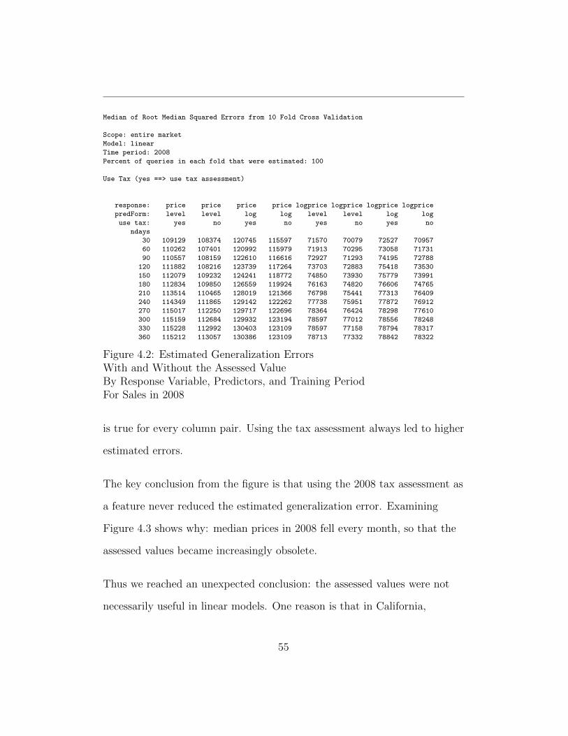
Figure 4.2 contains the results from the cross validation study. Column one
states the number of days in the training period. Each cell after column one
contains the median of the RMSE values from 10-fold cross validation. Here
RMSE means the square root of the median squared errors. Thus each cell
contains an estimate of the generalization error.
Column two contains estimated errors for the level-level form of the model,
which estimates price, and features that use the tax assessment. Column
three is also for the level-level form of the model, but does not use the tax
assessment.
Comparing columns two and three, we see that in every case the estimated
errors are lower if we do not use the tax assessment-derived features. This
54
Median of Root Median Squared Errors from 10 Fold Cross Validation
Scope: entire market
Model: linear
Time period: 2008
Percent of queries in each fold that were estimated: 100
Use Tax (yes ==> use tax assessment)
response: price price price price logprice logprice logprice logprice
predForm: level level log log level level log log
use tax: yes no yes no yes no yes no
ndays
30 109129 108374 120745 115597 71570 70079 72527 70957
60 110262 107401 120992 115979 71913 70295 73058 71731
90 110557 108159 122610 116616 72927 71293 74195 72788
120 111882 108216 123739 117264 73703 72883 75418 73530
150 112079 109232 124241 118772 74850 73930 75779 73991
180 112834 109850 126559 119924 76163 74820 76606 74765
210 113514 110465 128019 121366 76798 75441 77313 76409
240 114349 111865 129142 122262 77738 75951 77872 76912
270 115017 112250 129717 122696 78364 76424 78298 77610
300 115159 112684 129932 123194 78597 77012 78556 78248
330 115228 112992 130403 123109 78597 77158 78794 78317
360 115212 113057 130386 123109 78713 77332 78842 78322
Figure 4.2: Estimated Generalization ErrorsWith and Without the Assessed ValueBy Response Variable, Predictors, and Training PeriodFor Sales in 2008
is true for every column pair. Using the tax assessment always led to higher
estimated errors.
The key conclusion from the figure is that using the 2008 tax assessment as
a feature never reduced the estimated generalization error. Examining
Figure 4.3 shows why: median prices in 2008 fell every month, so that the
assessed values became increasingly obsolete.
Thus we reached an unexpected conclusion: the assessed values were not
necessarily useful in linear models. One reason is that in California,
55

Figure 4.3: Median PriceBy Month
For 2006 Through 2009
●
●
●
●
●
●
●
●
●
●
●
●
●
●
●
●
●
●
●
●
●
●
●
●
●
●
●
●
●
●
●
●
●
●
●
●
●
●
●2009−03
2009−02
2009−01
2008−12
2008−11
2008−10
2008−09
2008−08
2008−07
2008−06
2008−05
2008−04
2008−03
2008−02
2008−01
2007−12
2007−11
2007−10
2007−09
2007−08
2007−07
2007−06
2007−05
2007−04
2007−03
2007−02
2007−01
2006−12
2006−11
2006−10
2006−09
2006−08
2006−07
2006−06
2006−05
2006−04
2006−03
2006−02
2006−01
0e+00 2e+05 4e+05 6e+05median price
year
−m
onth
Proposition 13 biases the assessed values to be less than market values on
some properties but not others. Another reason is that the assessment may
become obsolete if market values are either increasing or decreasing
rapidly.
56

4.4 Understanding the Census Data
The United States Census Bureau conducts [Burb] a decennial census every
10 years. The year 2000 census [Bur02, p. 140] began in March 2000 to
survey all 98 million households. The survey technique was to mail surveys
and follow up with non-respondents by sending “enumerators” to the
household.
Two survey forms were used in 2000.
• Short-form: Most households (83 percent) received a questionnaire
asking for information on “name, sex, age, relationship, Hispanic
origin, and race.”
• Long-form: Some households (17 percent) received a questionnaire
that asked for both the short-form information and an additional “52
questions requesting . . . information about housing, social, and
economic characteristics of the household.”
Data were captured for each household and then aggregated for reporting
purposes. The lowest level of aggregation was the census block. Data from
census blocks were further aggregated into several hierarchies [Burc]. The
hierarchy of interest to this work had these levels: nation, region, divisions,
states, counties, census tracts, block groups, and census blocks. All of the
census data we used were from the 2000 census for Los Angeles County and
57

were at the census tract level.
Boundaries between census tracts in Los Angeles changed between the 2000
and 2010 censuses [Pro14]. That’s because census tracts are designed to
contain about 4,000 people: as populations grow and shrink, census tracts
need to be redefined. Indeed, an analysis of Los Angeles County census
data at the census tract level for years 1990 and 2000 shows an increase in
the number of census tracts in Los Angeles County, consistent with an
increase in the Los Angeles County population.
Unfortunately, the census tract numbers we used for properties were
contained in the tax roll, which we had only for 2008. Thus we could not
easily determine census tract numbers for parcels for the 1980 nor 1990
censuses. The implication was that the earliest date we could use the
census data we had was for the date when it first became available.
According to the help line for the Census Bureau, the year 2000 census
data became public sometime in 2002. Rather than determine that date
exactly, we assumed that transactions on or after January 1, 2003 properly
reflect census data from the year 2000 census.
58

4.5 Assessing the Predictive Power of the
Census Data
To assess whether features derived from the year 2000 census were valuable,
we used 10-fold cross validation to estimate the generalization error for a
variety of linear models, all trained and tested on data from 2003 on. The
models varied the same design choices as for the experiments to understand
the predictive power of features derived from the 2008 tax assessment.
These choices were:
• response variable: predict either the price or the logarithm of the
price.
• prediction variable forms: use as predictors either the natural units of
the predictors (called “level” in the chart) or the logarithm of the
natural units.
• number of training days: vary the training period from 30 days to 360
in steps of 30 days.
Figure 4.4 shows the estimated generalization error for each of the design
choices, both with and without the features derived from the census data.
The comparison metric is the median of the root median squared errors
from the folds. The key finding was that using the census-derived features
59

Median of Root Median Squared Errors from 10 Fold Cross Validation
Scope: entire market
Model: linear
Time period: 2003 on
Percent of queries in each fold that were estimated: 100
Column Use Cen (yes ==> use census data)
response: price price price price logprice logprice logprice logprice
predForm: level level log log level level log log
use cen: yes no yes no yes no yes no
ndays
30 75333 94172 81834 110373 58862 75280 59385 79074
60 74459 93202 81091 109280 58871 75378 59432 78694
90 74173 92533 80795 108732 59361 75324 59780 78864
120 74239 92238 80821 108479 60006 75647 60473 79088
150 74399 92036 80835 108197 60780 76125 61205 79412
180 74764 92042 81044 107796 61580 76456 62010 79935
210 75150 92053 81292 107460 62563 77022 62951 80212
240 75573 92063 81406 107142 63526 77521 63800 80881
270 75869 92092 81781 106993 64673 78202 65012 81459
300 76238 92237 82165 106989 65905 78948 66104 81931
330 76844 92544 82455 106823 67198 79713 67370 82644
360 77560 92658 82888 106680 68452 80652 68506 83404
Figure 4.4: Estimated Generalization ErrorsWith and Without Census Data By Response Variable, Predictors, andTraining Period
always led to better performance.
4.6 Discarding Assessments and Keeping
Census Data
Because the assessment data were not valuable for the time period for
which they were relevant, namely the year 2008, we decided to discard all
features derived from the assessment. This decision reduced our available
60

feature set and allowed us to use transactions before and after 2008.
Because the census data were valuable for the time period in which they
were relevant, namely beginning in 2003, we decided to keep these features
and restrict the analysis to year 2003 and later. The resulting dataset had
about 250,000 transactions. The median price over the time period was
$475,000.
61

Chapter 5
Finding the Best Linear
Model
Linear models predict the price as a linear function of features:
price = β0 + β1x1 + . . .+ βnxn.
From this simple idea, a huge variety of models can be generated. Which
linear models were most accurate for predicting the prices of houses?
We answered this question by examining data from 2003 and later using the
decennial census from the year 2000 but not the tax assessment for 2008.
Our interest was in estimating the generalization error for unseen
62

transactions. For this, we used 10-fold cross validation.
Property descriptions came from the tax roll for the year 2008. The tax roll
contained property descriptions as of October 31, 2007. We needed to
exclude from our data any houses built or modified after that date. An
analysis showed that there were no such houses.
All of the linear models in this chapter are local linear models, by which we
mean that a separate model was fitted for each query transaction. The
overall effect is to convert the linear models into an aggregate non-linear
model.
The plan of attack is reflected in the sections that follow.
• Section 1 explains our choice of metric to compare models. We show
that using different metrics leads to judging that different models
were better. We decided to focus on median errors.
• Section 2 studies design choices for local linear models that cover the
entire market. We started by considering model forms and the
number of training days that led to the most accurate models. (The
term “model form” captures whether transformations into the log
domain were used in the left hand and right hand sides of the model.
More on this later.) Having fixed form and number of training days,
we then considered which features were best and compared heuristics
63

for selecting the best features. Finally, fixing form, number of training
days, and feature sets, we showed that regularization improves
estimation accuracy.
• Section 3 considers submarket models. Submarket models partition
the possibly queries and use the partitions in the fitting and
prediction processes. We considered both indicator-based submarket
models, in which the submarkets are represented by indicator
variables in a single model for all queries, and separate submarket
models, in which a separate model was built for each submarket. We
considered multiple definitions for submarkets. We found that
submarket models outperformed entire-market models.
• Section 4 summarizes our results for local linear models and provides
some guidelines for extending the work into a commercial setting.
• Section 5 compares the results from the local linear models with a
random forests model. We show that the local linear model was
outperformed by the random forests model.
5.1 Figure of Merit
The literature often compares models using the fraction of estimates within
10 percent of the known values. The motivation for this figure of merit may
64

in part be that Freddie Mac is said [FLM03, footnote on p. 642] to use that
metric to judge the effectiveness of automated valuation models. In any
case, using fraction within 10 percent (along with fraction within 20 and 30
percent) is popular in the real estate pricing literature.
It is a curious choice of metric for at least two reasons. The first reason is
that linear models are often trained to minimize the mean squared error.
So fraction within 10 percent isn’t the criteria the model was trained to
deliver. The second reason is that selecting fraction within x percent is
implicitly a decision to favor models that are close when accurate and to
not minimize the average error.
Here’s a contrived example which illustrates that point. There are two
properties both of which sold for $100,000. Suppose we have two models to
consider. Model A produces estimates of $100,000 and $200,000. It is either
perfect or very wrong. Model B produces estimates of $85,000 and
$115,000. It is never super accurate but never very wrong. Model A has 50
percent of its estimates within 10 percent of the true value, Model B has 0
percent of its estimates within 10 percent of the true value. So under the
fraction-with-x-percent metric, we prefer model A over model B.
Now imagine using model A. When it delivers its estimate, we have no idea
whether the estimate is good or bad. To me, this situation is untenable if
there is an acceptable alternative (and there is: use some variant on mean
65

squared error). To make the untenable situation acceptable, one would
need to produce both an estimate and a confidence in the estimate. Now
the model has to be trained to deliver two values, and we have conceivably
more than doubled the difficulty of the problem of selecting the best model:
there are now two figures of merit and how to make tradeoffs between them
is not obvious.
The issue of choice of figure of merit would be moot if using either metric
resulted in selecting the same model as best. To investigate whether the
issue is moot, we designed an experiment. In the experiment, we considered
the estimated generalization error from a variety of models. The models
were generated by sweeping these design choices:
• Response variable: either the price or log(price)
• The form of the predictors: either level (natural units) or log of
natural units for size features
• The number of days in the training period, from 30 up to 360 in steps
of 30 days
• The figure of merit used to select the model: one of the mean of the
root mean squared errors from the folds (meanRMSE in the figure), the
median of the root median squared errors from the folds (medRMSE),
or the fraction within 10 percent of actual values (fctWI10).
66

All of these models used all features always present except for those derived
from the tax assessor data. All models used data from 2003 on.
The results are depicted in Figure 5.1.
The table has two panels. In panel A, the response variable is price. In
panel B the response variable is log(price). Each panel has a row for each
training period considered. The length of the training period is in column
ndays. Adjacent to the training period are two groups of columns. The
first group is for the level form of the predictors: we used the predictors in
their natural units. The second group is for the log form of the predictors:
we transformed the size features into the log domain. Each group of three
columns has the estimated error using one of the metrics. Our interest was
to determine which model was best. For the first two metrics, meanRMSE
and medRMSE, we sought the lowest error. For the third, fctWI10, we sought
the highest accuracy.
You will notice very high value in Panel B, column 2. These are the
estimated errors using the meanRMSE metric for the log-level form of the
linear model. What is happening is that a few houses were very badly
predicted. These houses tended to have unusually large values for some
features, causing the log(price) estimate to be very much higher than the
actual transaction price.
67

Comparison of Metrics From from 10 Fold Cross Validation
Mean of Root Mean Squared Errors Across Folds (meanRMSE)
Median of Root Median Squared Errors Across Folds (medRMSE)
Mean of Fraction of Predictions Within 10 Percent of Actual Across Folds (fctWI10)
Scope: entire market
Model: linear
Time period: 2003 on
Predictors: always in every transaction and not in the tax assessment
Percent of queries in each fold that were estimated: 100
Panel A: price
predictorsForm: level level level log log log
metric: meanRMSE medRMSE fctWI10 meanRMSE medRMSE fctWI10
ndays
30 638476 75333 0.339 252444 81834 0.315
60 395434 74459 0.341 251268 81091 0.318
90 447337 74173 0.342 251148 80795 0.319
120 244367 74239 0.341 251260 80821 0.319
150 247197 74399 0.340 251520 80835 0.319
180 242215 74764 0.339 251892 81044 0.318
210 242706 75150 0.337 252337 81292 0.318
240 243262 75573 0.335 252837 81406 0.316
270 243764 75869 0.332 253343 81781 0.315
300 244292 76238 0.330 253893 82165 0.314
330 244892 76844 0.327 254478 82455 0.312
360 245459 77560 0.324 255058 82888 0.310
Panel B: logprice
predictorsForm: level level level log log log
metric: meanRMSE medRMSE fctWI10 meanRMSE medRMSE fctWI10
ndays
30 Inf 58862 0.413 254065 59385 0.407
60 1e+113 58871 0.411 253161 59432 0.406
90 2e+63 59361 0.407 253140 59780 0.403
120 8e+10 60006 0.402 253135 60473 0.399
150 4e+22 60780 0.397 253264 61205 0.394
180 1e+06 61580 0.391 253451 62010 0.388
210 1e+06 62563 0.385 253785 62951 0.382
240 2e+06 63526 0.379 254167 63800 0.376
270 2e+06 64673 0.372 254528 65012 0.370
300 2e+06 65905 0.366 255025 66104 0.364
330 2e+06 67198 0.358 255488 67370 0.357
360 2e+06 68452 0.351 255992 68506 0.351
Figure 5.1: Estimated Generalization ErrorsFor Model Selection MetricsBy Response Variable, Predictors, and Training PeriodsFor Sales in 2003 and Later
68

best ndaysform meanRMSE medRMSE fctWI10
level-level 180 90 90level-log 90 90 120log-level 195 30 30log-log 120 30 30
Figure 5.2: Preferred Number of Training DaysBy Model Selection MetricFor Model FormsSummarizing Figure 5.1
It was always true that the expected loss for the metric meanRMSE greatly
exceeded that for medRMSE. This was because there was right-skew in the
prices: the mean exceeds the median, so that the mean error can exceed the
median error.
We wanted to answer the question: which model was selected as best by
each metric? Figure 5.2 contains these results.
There are several observations to make:
• In no cases, did all three metrics pick the same number of training
days.
• The metrics medRMSE and fctWI10 closely agreed on the best number
of training days. They agreed on all model forms except for the
level-log form, and there they were only 30 days apart.
• The metric meanRMSE usually picked more training days as optimal
69

than did the other metrics.
We concluded that the choice of metric did influence the choice of the best
training period to use.
Going forward, we focused on the medRMSE metric, judging that it more
intuitively sizes average errors than did meanRMSE (because of the
right-skew in the prices) and reflecting our predisposition to minimize
average errors rather than accuracy.
5.2 Entire-market Models
This section explores linear models that are specified once for the entire
marketplace: there is one model for every query transaction and this model
is location aware only through features of the census tract and zip code of
the property. I call these kinds of models “entire-market models.”
Within the class of entire-market models, we explored design choices. In
the first subsection that follows, we examine the form of the equation in the
model and the training period used to fit the model. We found that training
using 30 days of data before the query transaction was best. The best form
of model to use was log-level, so that one would predict the log of price
using the features in natural units. In the subsequent subsection, we then
examine, within this choice of training period and form, which features gave
70

the best predicted performance and examine a reduced-feature model. We
found that a 15-feature model performed best. In the final subsection, we
examine adding an L2 regularizer to the 15-feature model. We found that
adding the regularizer improved performance slightly.
5.2.1 Model form and number of training days
In the literature, a popular model form is the log-level form: one predicts
log(price) using features in their natural units. Other choices for model
form include log-log, in which the log of price is predicted using size
features that are in the log domain and non-size features in their natural
units, level-level in which price is predicted using features in their natural
units, and level-log in which price is predicted using size features in the log
domain and non-size features in their natural units.
At least four rationales can be invoked to choose a model form. First is
that the form of the model should conform to one’s prior assumptions
about the data generation process. If you suppose that doubling the lot size
might double the price, you can admit this possibility by specifying
log(price) = β log(size), a log-log form. If you suppose that adding a
bedroom adds a certain amount of value, you would want to have
price = β bedrooms, a level-level form.
A second rationale for choosing the form is to transform the prices to a
71

form more compatible with the statistical assumptions of the model. Since
real estate prices tend to be right-skewed, a log transformation would
possibly make the transformed distribution more normal.
A third rationale is to transform the price to the log domain in order to
avoid applying equal importance with respect to prediction errors to
expensive and less expensive houses. By prediction log(price) instead of
price, the idea is to fit the model to minimize errors on the more typical,
less expensive houses, not to minimize the price-weighted error, which could
be regarded as overly influenced by a few very large houses.
We focused on a fourth rationale and simply asked: Which model form
yielded the lowest estimated generalization errors as measured by the
median of the root median squared error across folds?
Another issue was to determine the best training period. Linear models are
setting the marginal price of each feature. If prices are moving slowly, then
training on a longer period of time might be beneficial. If prices are moving
rapidly, then training only on recent data might be necessary.
Our experiment fixed the time period (2003 on) and the feature set (all
features always in transactions excluding the features derived from the tax
assessment). We varied the model form and number of training days and
built a local model for every query transaction in every training fold. The
local model was built by using the query date to discard transactions in
72
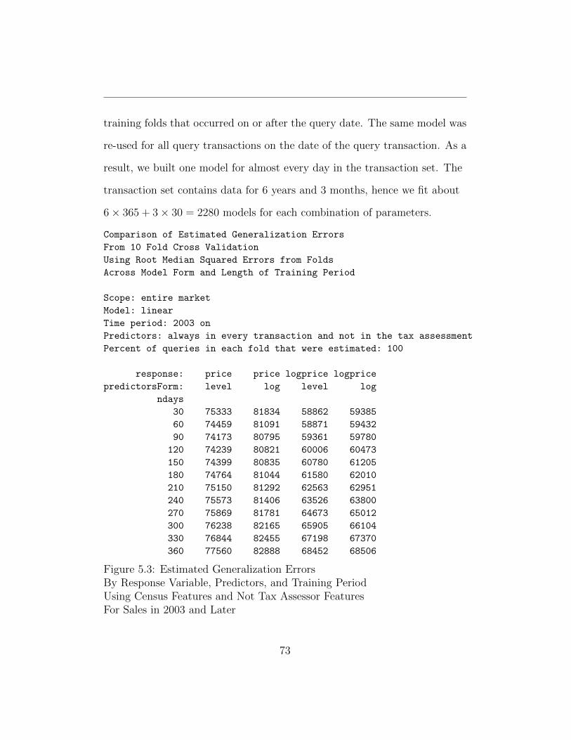
training folds that occurred on or after the query date. The same model was
re-used for all query transactions on the date of the query transaction. As a
result, we built one model for almost every day in the transaction set. The
transaction set contains data for 6 years and 3 months, hence we fit about
6× 365 + 3× 30 = 2280 models for each combination of parameters.
Comparison of Estimated Generalization Errors
From 10 Fold Cross Validation
Using Root Median Squared Errors from Folds
Across Model Form and Length of Training Period
Scope: entire market
Model: linear
Time period: 2003 on
Predictors: always in every transaction and not in the tax assessment
Percent of queries in each fold that were estimated: 100
response: price price logprice logprice
predictorsForm: level log level log
ndays
30 75333 81834 58862 59385
60 74459 81091 58871 59432
90 74173 80795 59361 59780
120 74239 80821 60006 60473
150 74399 80835 60780 61205
180 74764 81044 61580 62010
210 75150 81292 62563 62951
240 75573 81406 63526 63800
270 75869 81781 64673 65012
300 76238 82165 65905 66104
330 76844 82455 67198 67370
360 77560 82888 68452 68506
Figure 5.3: Estimated Generalization ErrorsBy Response Variable, Predictors, and Training PeriodUsing Census Features and Not Tax Assessor FeaturesFor Sales in 2003 and Later
73
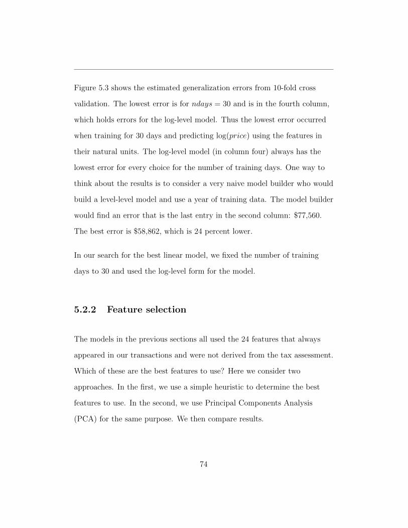
Figure 5.3 shows the estimated generalization errors from 10-fold cross
validation. The lowest error is for ndays = 30 and is in the fourth column,
which holds errors for the log-level model. Thus the lowest error occurred
when training for 30 days and predicting log(price) using the features in
their natural units. The log-level model (in column four) always has the
lowest error for every choice for the number of training days. One way to
think about the results is to consider a very naive model builder who would
build a level-level model and use a year of training data. The model builder
would find an error that is the last entry in the second column: $77,560.
The best error is $58,862, which is 24 percent lower.
In our search for the best linear model, we fixed the number of training
days to 30 and used the log-level form for the model.
5.2.2 Feature selection
The models in the previous sections all used the 24 features that always
appeared in our transactions and were not derived from the tax assessment.
Which of these are the best features to use? Here we consider two
approaches. In the first, we use a simple heuristic to determine the best
features to use. In the second, we use Principal Components Analysis
(PCA) for the same purpose. We then compare results.
74

LCV Heuristic
We had 24 features that were candidates for inclusion in the model. A
straight-forward way to determine the best feature set would have been to
consider all possible subsets and to have estimated the generalization error
for each. Doing so would have been way too time consuming, because there
were 224 possible feature sets to evaluate.
Our idea was to instead use L1 regularization to determine the rank
ordering of the 24 features in terms of their importance. We then used cross
validation to estimate the generalization error from a model with the first,
the first two, . . . , all 24 rank ordered features. We call the procedure LCV,
for L1 regularization followed by cross validation.
The implementation was by using the Elastic Net from Zoe and Hastie
[ZH05]. It fits a linear model while concurrently using an L1 and L2
regularizer. As a by-product, an R implementation, the elasticnet R
package [ZH], produces a rank ordering of the features in terms of their
importance. In our use of this package, we set the L2 regularizer to zero
and used just the rank ordering of features under the L1 regularizer.
The result of the rank ordering from the Elastic Net procedure is in Figure
5.4. It shows that the most important feature is the living area of the
house. Real estate agents often claim the most important feature of the
house is its location, but that wasn’t true in these data. Instead, features of
75

the location (median household income and average commute time) were
second and third in importance.
76
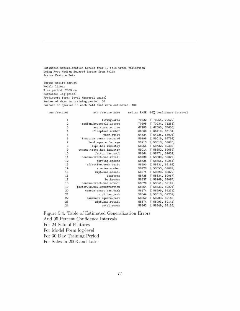
Estimated Generalization Errors from 10-fold Cross Validation
Using Root Median Squared Errors from Folds
Across Feature Sets
Scope: entire market
Model: linear
Time period: 2003 on
Response: log(price)
Predictors form: level (natural units)
Number of days in training period: 30
Percent of queries in each fold that were estimated: 100
num features nth feature name median RMSE 95% confidence interval
1 living.area 79332 [ 78954, 79679]
2 median.household.income 70595 [ 70234, 71288]
3 avg.commute.time 67185 [ 67005, 67656]
4 fireplace.number 66566 [ 66410, 67184]
5 year.built 64634 [ 64425, 65004]
6 fraction.owner.occupied 59198 [ 59019, 59793]
7 land.square.footage 59213 [ 58818, 59620]
8 zip5.has.industry 58955 [ 58732, 59386]
9 census.tract.has.industry 59014 [ 58852, 59659]
10 factor.has.pool 58864 [ 58771, 59624]
11 census.tract.has.retail 58730 [ 58589, 59329]
12 parking.spaces 58735 [ 58356, 59261]
13 effective.year.built 58590 [ 58331, 59184]
14 stories.number 58728 [ 58353, 59099]
15 zip5.has.school 58571 [ 58328, 58879]
16 bedrooms 58735 [ 58334, 59067]
17 bathrooms 58837 [ 58169, 59097]
18 census.tract.has.school 58826 [ 58341, 59142]
19 factor.is.new.construction 58854 [ 58333, 59201]
20 census.tract.has.park 58874 [ 58299, 59271]
21 zip5.has.park 58844 [ 58318, 59209]
22 basement.square.feet 58852 [ 58283, 59148]
23 zip5.has.retail 58874 [ 58293, 59141]
24 total.rooms 58862 [ 58349, 59155]
Figure 5.4: Table of Estimated Generalization ErrorsAnd 95 Percent Confidence IntervalsFor 24 Sets of FeaturesFor Model Form log-levelFor 30 Day Training PeriodFor Sales in 2003 and Later
77

●
●
●
●
●
●
●
●
●
●
●
●
●
●
●
●
●
●
●
●
●
●
●
●
●
●
●
●
●
●
●
●
●
●
●
●
●
●
●
●
●
●
●
●
●
●
●
●
●
●
●
●
●
●
●
●
●
●
●
●
●
●
●
●
●
●
●
●
●
●
●
●total.rooms
zip5.has.retail
basement.square.feet
zip5.has.park
census.tract.has.park
factor.is.new.construction
census.tract.has.school
bathrooms
bedrooms
zip5.has.school
stories.number
effective.year.built
parking.spaces
census.tract.has.retail
factor.has.pool
census.tract.has.industry
zip5.has.industry
land.square.footage
fraction.owner.occupied
year.built
fireplace.number
avg.commute.time
median.household.income
living.area
60000 65000 70000 75000 80000median rMedianSE across folds
cum
ulat
ive
feat
ure
nam
es
Figure 5.5: Graph of Estimated Generalization ErrorsAnd 95 Percent Confidence IntervalsFor 24 Sets of FeaturesFor Model Form log-levelFor 30 Day Training PeriodFor Sales in 2003 and Later
The same data are shown graphically in Figure 5.5, which displays the
estimated generalization error from including the first n features, together
with a 95 percent confidence interval. The large dots are the median of the
root median squared errors from the folds. The small dots to either side of
the large dots are the lower and upper bounds of the confidence intervals.
One sees that the lowest estimated error was when using the first 15
78

features, from living-area to zip5-has-school. The estimated errors then
tend to increase and the placement of the confidence intervals does not
compel one to consider going beyond the first 15 features.
If one seeks parsimony, one could consider using the first six features
(through fraction-owner-occupied), after which there was an increase in
estimated generalization error before a subsequent decline to the minimum
at 15 features.
Most important features
As found through L1 regularization
importance rank house feature location feature
1 living.area
2 median.household.income
3 avg.commute.time
4 fireplace.number
5 year.built
6 fraction.owner.occupied
7 land.square.footage
8 zip5.has.industry
9 census.tract.has.industry
10 factor.has.pool
11 census.tract.has.retail
12 parking.spaces
13 effective.year.built
14 stories.number
15 zip5.has.school
16 bedrooms
17 bathrooms
18 census.tract.has.school
19 factor.is.new.construction
20 census.tract.has.park
21 zip5.has.park
22 basement.square.feet
23 zip5.has.retail
24 total.rooms
Figure 5.6: 24 FeaturesBy Importance RankClassified as House Features or Location Features
Figure 5.6 shows the 24 rank-ordered features split into house features and
79

location features. Some observations on the house features:
• living-area: this is the interior living space. Construction is required
to change it, so I was not surprised to see it highly ranked. That it is
more highly ranked than the land square footage was a surprise to
me, because land square footage seems harder to change than interior
living space.
• fireplace-number: the number of fireplaces, including the possibility of
zero. A surprise—perhaps fireplaces are proxies for overall amenities
in the house.
• year-built: the year the house was built. Other studies have
concluded that the age and the squared age of the house are
important features. Our models were local, so that we needed a
house’s age for every query transaction. Instead of pre-building a
training set for each possible query, we transformed year built into
age and age squared just before fitting the model. We performed a
similar transformation for the effective year built, which is the last
year of significant updates to the house.
• factor-has-pool: whether there is a swimming pool. Not a surprise, as
the houses were all in Los Angeles, where the weather is often
pleasant and a swimming pool might be a joy.
80

Some observations on the location features:
• median-household-income and fraction-owner-occupied: the median
income in the census tract from the year 2000 census and the fraction
of houses in the census tract that were occupied by owners. Both of
these features indicated the wealth of the neighborhood.
• average-commute-time: in other studies, longer commutes were
associated with lower prices.
• zip5-has-industry and census-tract-has-industry: being near industry
was not good for house prices.
• census-tract-has-park and zip5-has-park: Los Angeles residents were
not there for the parks. Perhaps this is because it is a driving-around
city, not a walking-around city.
PCA
The second approach we used to determine the importance of features was
Principal Components Analysis. Figure 5.7 shows the principal components
associated with the training set predictors. The first three principal
components accounted for almost 100 percent of the variance.
In Figure 5.8 we see the weights of the 24 features in the first principal
81

PCA Principal Component Variances
Principal Component 1 Variance 519224186 Cum Fraction Total Variance 0.929503
Principal Component 2 Variance 23925994 Cum Fraction Total Variance 0.972335
Principal Component 3 Variance 15156837 Cum Fraction Total Variance 0.999468
Principal Component 4 Variance 293190 Cum Fraction Total Variance 0.999993
Principal Component 5 Variance 2492 Cum Fraction Total Variance 0.999998
Principal Component 6 Variance 952 Cum Fraction Total Variance 0.999999
Principal Component 7 Variance 354 Cum Fraction Total Variance 1.000000
Principal Component 8 Variance 30 Cum Fraction Total Variance 1.000000
Principal Component 9 Variance 14 Cum Fraction Total Variance 1.000000
Principal Component 10 Variance 1 Cum Fraction Total Variance 1.000000
Principal Component 11 Variance 0 Cum Fraction Total Variance 1.000000
Principal Component 12 Variance 0 Cum Fraction Total Variance 1.000000
Principal Component 13 Variance 0 Cum Fraction Total Variance 1.000000
Principal Component 14 Variance 0 Cum Fraction Total Variance 1.000000
Principal Component 15 Variance 0 Cum Fraction Total Variance 1.000000
Principal Component 16 Variance 0 Cum Fraction Total Variance 1.000000
Principal Component 17 Variance 0 Cum Fraction Total Variance 1.000000
Principal Component 18 Variance 0 Cum Fraction Total Variance 1.000000
Principal Component 19 Variance 0 Cum Fraction Total Variance 1.000000
Principal Component 20 Variance 0 Cum Fraction Total Variance 1.000000
Principal Component 21 Variance 0 Cum Fraction Total Variance 1.000000
Principal Component 22 Variance 0 Cum Fraction Total Variance 1.000000
Principal Component 23 Variance 0 Cum Fraction Total Variance 1.000000
Principal Component 24 Variance 0 Cum Fraction Total Variance 1.000000
Figure 5.7: Cumulative Variance of the 24 Principal Components
component. The median household income had the highest absolute weight.
Other weights were much lower in absolute value. The only ones of much
importance were the land square footage and the living area. It seemed
that the first principal component may have been about the wealth of the
neighborhood.
In Figure 5.9 we see the weights of the 24 features in the second principal
component. The land square footage had the highest absolute weight.
Other weights were much lower in value with household income and living
area being the largest in absolute size. This principal component was
possibly about the size of the land.
82

PCA Rotation for Principal Component 1
Feature avg.commute.time Weight -0.000005
Feature census.tract.has.industry Weight +0.000007
Feature census.tract.has.park Weight -0.000000
Feature census.tract.has.retail Weight +0.000005
Feature census.tract.has.school Weight +0.000001
Feature fraction.owner.occupied Weight -0.000006
Feature median.household.income Weight -0.996050
Feature basement.square.feet Weight +0.000112
Feature bathrooms Weight -0.001563
Feature bedrooms Weight -0.000009
Feature effective.year.built Weight -0.000210
Feature factor.has.pool Weight -0.000004
Feature factor.is.new.construction Weight +0.000000
Feature fireplace.number Weight -0.000009
Feature land.square.footage Weight -0.087663
Feature living.area Weight -0.014042
Feature parking.spaces Weight -0.000006
Feature stories.number Weight -0.000353
Feature total.rooms Weight -0.000019
Feature year.built Weight -0.000212
Feature zip5.has.industry Weight +0.000005
Feature zip5.has.park Weight -0.000000
Feature zip5.has.retail Weight +0.000000
Feature zip5.has.school Weight +0.000001
Figure 5.8: Feature Weights For the First Principal Component
In Figure 5.10 we see the weights of the 24 features for third principal
component. It was mostly composed of the basement square feet, perhaps a
proxy for other size features in the house: bigger basement probably implies
bigger house. This principal component was possibly about the size of the
house.
In Figure 5.11 we see the estimated generalization error from using the
median household income, land square footage, and so on up to the 4
features identified as important in the PCA work. The same data are in
Figure 5.12 which shows the 95 percent confidence intervals graphically.
The lowest estimated error was from using the first 3 features. Adding
83

PCA Rotation for Principal Component 2
Feature avg.commute.time Weight +0.000124
Feature census.tract.has.industry Weight +0.000002
Feature census.tract.has.park Weight -0.000000
Feature census.tract.has.retail Weight -0.000002
Feature census.tract.has.school Weight +0.000008
Feature fraction.owner.occupied Weight -0.000001
Feature median.household.income Weight -0.088131
Feature basement.square.feet Weight +0.004862
Feature bathrooms Weight +0.003195
Feature bedrooms Weight +0.000021
Feature effective.year.built Weight +0.000200
Feature factor.has.pool Weight +0.000013
Feature factor.is.new.construction Weight -0.000000
Feature fireplace.number Weight +0.000020
Feature land.square.footage Weight +0.995409
Feature living.area Weight +0.036884
Feature parking.spaces Weight +0.000019
Feature stories.number Weight +0.000164
Feature total.rooms Weight +0.000044
Feature year.built Weight +0.000188
Feature zip5.has.industry Weight +0.000001
Feature zip5.has.park Weight +0.000001
Feature zip5.has.retail Weight -0.000001
Feature zip5.has.school Weight +0.000000
Figure 5.9: Feature Weights For the Second Principal Component
basement-square-feet slightly increased the estimated error but yielded a
smaller 95 percent confidence interval, so some may prefer keeping the
fourth PCA feature.
Reduced Feature Models
To find the best reduced-feature model, we tested all the feature sets
suggested by the LCV and PCA analyses. These results are in Figure 5.13,
which brings together results previously shown. The PCA-derived feature
sets all underperformed the LCV-derived feature sets: extremely small
feature sets were challenged in this setting. The best feature set was the
84

PCA Rotation for Principal Component 3
Feature avg.commute.time Weight -0.000000
Feature census.tract.has.industry Weight -0.000000
Feature census.tract.has.park Weight -0.000000
Feature census.tract.has.retail Weight +0.000000
Feature census.tract.has.school Weight -0.000000
Feature fraction.owner.occupied Weight -0.000000
Feature median.household.income Weight +0.000534
Feature basement.square.feet Weight +0.999988
Feature bathrooms Weight +0.000060
Feature bedrooms Weight -0.000000
Feature effective.year.built Weight -0.000007
Feature factor.has.pool Weight -0.000000
Feature factor.is.new.construction Weight -0.000000
Feature fireplace.number Weight +0.000000
Feature land.square.footage Weight -0.004849
Feature living.area Weight +0.000320
Feature parking.spaces Weight +0.000000
Feature stories.number Weight -0.000004
Feature total.rooms Weight +0.000001
Feature year.built Weight -0.000016
Feature zip5.has.industry Weight +0.000000
Feature zip5.has.park Weight -0.000000
Feature zip5.has.retail Weight +0.000000
Feature zip5.has.school Weight +0.000000
Figure 5.10: Feature Weights For the Third Principal Component
Estimated Generalization Errors from 10-fold Cross Validation
Using Root Median Squared Errors from Folds
Across Feature Sets
Scope: entire market
Model: linear
Time period: 2003 on
Response: log(price)
Predictors form: level (natural units)
Number of days in training period: 30
Percent of queries in each fold that were estimated: 100
num features nth feature name median RMSE 95% confidence interval
1 median.household.income 91623 [ 90463, 91891]
2 land.square.footage 87125 [ 86052, 87505]
3 living.area 70369 [ 70174, 71175]
4 basement.square.feet 70388 [ 70144, 70973]
Figure 5.11: Table of Estimated Generalization Errors and 95 Percent Con-fidence IntervalsFor Feature Sets Selected by the PCA Analysis
85
●
●
●
●
●
●
●
●
●
●
●
●basement.square.feet
living.area
land.square.footage
median.household.income
70000 75000 80000 85000 90000median rMedianSE across folds
cum
ulat
ive
feat
ure
nam
es
Figure 5.12: Graph of Estimated Generalization Errors and 95 Percent Con-fidence IntervalsFor Feature Sets Selected by the PCA Analysis
one with the first 15 features from the LCV heuristic. This feature set had
an estimated error of $58,571, which was 17 percent lower that the
estimated error of $70,369 which was found by PCA.
5.2.3 Regularization
Regularizing models is one way to avoid overfitting and thereby improve
prediction accuracy. So far the models were not regularized.
86

●
●
●
●
●
●
●
●
●
●
●
●pca04
pca03
best15
best06
0 20000 40000 60000median rMedianSE across folds
pred
icto
r fe
atur
e se
t nam
es
Figure 5.13: Graph of Estimated Generalization Errors and 95 Percent Con-fidence IntervalsFor Feature Sets Selected by the LCV and PCA Analyses
To assess the extent to which regularization led to more accuracy, we took
the model using the 15 best features and ran multiple versions using several
choices for the weight of the L2 regularizer. A simple line search was
used.
Figure 5.14 contains the result in a table. We see the typical pattern:
increasing the regularizer weight first decreased errors and as the weight
continued to increase, errors were increased. Setting the weight to λ = 55
87

Estimated Generalization Errors from 10-fold Cross Validation
L2 regularizer value median 95% confidence interval
0 58622 [ 58367, 58897]
1 58619 [ 58357, 58895]
2 58618 [ 58392, 58922]
3 58620 [ 58392, 58906]
4 58617 [ 58385, 58929]
5 58620 [ 58344, 58960]
6 58622 [ 58374, 58971]
7 58596 [ 58366, 58967]
8 58591 [ 58382, 58938]
9 58583 [ 58366, 58920]
10 58603 [ 58363, 58911]
30 58463 [ 58236, 58960]
41 58490 [ 58240, 58920]
55 58453 [ 58166, 58957]
74 58475 [ 58128, 58914]
100 58459 [ 58199, 59011]
132 58540 [ 58252, 58943]
173 58537 [ 58278, 59054]
228 58735 [ 58364, 59217]
300 58971 [ 58641, 59306]
1000 61919 [ 61388, 62108]
3000 69387 [ 69112, 69946]
10000 85187 [ 84669, 85687]
Figure 5.14: Estimated Generalization Errors and 95 Percent ConfidenceIntervalsFor Selected L2 Regularizers
seemed like a good choice: it had the lowest median across the
cross-validation folds and from Figure 5.15, one can see the 95 percent
confidence intervals were not signaling warnings.
The impact of the regularizer on the estimated generalization error was
very small: the median was reduced by $169 from an unregularized error of
$58,622, a reduction of less than three-tenths of a percent. The small
impact of the regularizer suggests that there was not much overfitting in
the unregularized model. Perhaps this was because the models were all
88

●
●
●
●
●
●
●
●
●
●
●
●
●
●
●
●
●
●
●
●
●
●
●
●
●
●
●
●
●
●
●
●
●
●
●
●
●
●
●
●
●
●
●
●
●
●
●
●
●
●
●
●
●
●
●
●
●
●
●
●
●
●
●
●
●
●
●
●
●10000
3000
1000
300
228
173
132
100
74
55
41
30
10
9
8
7
6
5
4
3
2
1
0
60000 70000 80000Estimated Generalization Errors
L2 r
egul
ariz
er v
alue
Figure 5.15: Estimated Generalization Error from L2 Regularization
local models.
5.3 Submarket Models
We considered three very simple definitions of submarkets. In the first, the
submarkets were defined by the census tracts. Each census tract was its
own submarket. In the second, submarkets were defined by the city names.
Each city was its own submarket. In the third, submarkets were defined by
89

zip code. Each five-digit zip code was its own submarket.
We considered two approaches to incorporating submarkets into the model.
The first used indicator variables, the second built a separate model for
each submarket.
5.3.1 Using Indicator Variables
The indicator models all had indicators for whether the observation was in
a specific submarket. For example, for zip-code based submarkets, the
model was
log(price) = β0 + β1ZipIs11111 + β2ZipIs22222 + . . .
+ βkLotSize+ βk+1LivingArea+ . . . .
The indicators were capturing the possibly different average prices in each
submarket. The average price per feature was the same across
submarkets.
Figure 5.16 shows the estimated generalization errors from adding
indicators variables to the regularized linear model. We see that adding
indicators for zip codes, census tract, and cities all helped and that the best
90

Estimated Generalization Errors from 10-fold Cross Validation
Using Median of Root Median Squared Errors from Folds
Across Indicator Models
Model: linear with L2 regularizer
Time period: 2003 on
Response: log(price)
Predictors form: level (natural units)
Percent of queries in each fold that were estimated: 100
Number of days in training period: 30
Lambda: 55.00
indicators for medRMSE ci95%.lo ci95%.hi
no indicators 58453 58169 58957
zip 5 code 41013 40669 41287
census tract 45662 45451 45956
city 44521 44160 44642
Figure 5.16: Estimated Generalization Errors and 95 Percent ConfidenceIntervalsFor Submarket Indicators
result was obtained with the five-digit zip code indicators, which had an
error rate 30 percent lower than the entire-market model (the model with
no indicators).
5.3.2 Separate Models for Each Submarket
The separate-models approach built a separate model for each submarket.
Each model had the same form:
log(price) = β0 + βkLotSize+ βk+1LivingArea+ . . . .
A query transaction was presented, its submarket was determined, for
91

example, it was in zip code 11111, and then a model was trained using only
transactions in the prior 30 days in the zip code. This fitted model was
used to estimate the value for the query transaction.
This fitting process resulted in many models that could not be estimated,
most often because there were too few transactions in the training set.
Estimated Generalization Errors from 10-fold Cross Validation
Using Median of Root Median Squared Errors from Folds
Across Submarket Models
Model: linear with L2 regularizer
Time period: 2003 on
Response: log(price)
Predictors form: level (natural units)
Percent of queries in each fold that were estimated: 100
Number of days in training period: 30
Lambda: 55.00
scope name medRMSE 95%ci.low 95%ci.hi nScope nAlways coverage
census.tract 53635 50742 57245 1950 1047 0.54
property.city 46405 42021 51839 191 126 0.66
zip5 55436 50401 61862 331 279 0.84
Figure 5.17: Estimated Generalization Errors and 95 Percent ConfidenceIntervalsFor Submarket Models
Figure 5.17 shows the results of this experiment. The submarket models
that used city names had the lowest estimated generalization error, which
was 21 percent lower than the whole-market error (the model from the
previous figure with no indicators). The fitting process, however, succeeded
in all folds in only 66 percent of the city names. (We defined “covered” to
mean that at least one model for the submarket could be fit in every test
fold. We defined “coverage” to be the fraction of possible submarkets that
were covered.) In terms of the estimated error, the worst model was for zip
92

codes, but it had the highest coverage. The lowest coverage was for census
tracts.
Perhaps the city names had the lowest errors because cities may acquire
brand positioning: they stand for something. Whatever that something is,
it attracts buyers who have affinity for that something, reinforcing the
positioning. The reinforcement leads to homogeneity within a city and that
makes it easier to fit the linear models.
Coverage numbers could be increased most likely by either retraining the
models on more than 30 days of data or forming submarket groups by
splicing together some of the submarkets. The latter approach has been
tried in the literature. The former appears not to have been tried.
Comparing Figures 5.16 and 5.17 we see that the best indicator model had
an error of $41,013, which was lower than the $46,405 error for the city
model. I was surprised by this, because the indicator-based models were
simply adjusting the average price level for each area and the submarket
models have the freedom to adjust the value of each feature in each
submarket.
The estimated errors in Figure 5.17 are perhaps deceptive: they are the
median values across all the submarkets. Individual models for specific
submarkets may have much lower or higher errors than the median for all
markets.
93

Example of Estimated Generalization Errors from 10-fold Cross Validation
Using Median of Root Median Squared Errors from Folds
Examples of Models for Scope Property City
scope name medRMSE
lowest 10 medians
LANCASTER 14937
PALMDALE 17884
LAPUENTE 23324
ARLETA 24078
NORWALK 24353
POMONA 24786
COMPTON 24909
LAKEWOOD 25610
SOUTHGATE 25615
PANORAMACITY 26105
middle 10 medians
CASTAIC 44870
NORTHRIDGE 44990
HAWAIIANGARDENS 45194
COMMERCE 45486
DOWNEY 45503
ALHAMBRA 46008
HAWTHORNE 46802
TUJUNGA 46839
LONGBEACH 47381
NORTHHOLLYWOOD 48431
highest 10 medians
MANHATTANBEACH 263123
LACANADA 269054
HIDDENHILLS 273258
TOLUCALAKE 290696
SANTAMONICA 297360
BEVERLYHILLS 306666
HERMOSABEACH 358661
MARINADELREY 385632
PACIFICPALISADES 395398
MALIBU 574980
Figure 5.18: Estimated Generalization ErrorsFor Selected Property City Submarket ModelsUsing Metric Median of Root Median Squared Errors
Let’s focus on the city-defined submarkets, which had the lowest median
errors. Error estimates were produced for 126 cities. The median errors for
each city varied widely. Figure 5.18 shows the medians for various cities.
We see that the most accurately-estimated houses were those in Lancaster,
94

where the estimated generalization error was about $15,000. A common
attribute of the cities with the ten lowest errors was that they all had
relatively low-priced houses. Median house prices for them from 2003
through 2009 ranged from $220,000 to $405,000.
Turning to the cities with the ten highest estimated errors, we see cities
that were expensive: Santa Monica, Beverly Hills, Malibu. The median
prices in this group of cities ranged from $1.0 million to $2.1 million (for
Hidden Hills).
The larger estimated errors for the more expensive cities may have been
generated in part from the higher prices, so that a 10 percent error in an
estimate was a larger amount than for lower-priced cities. Another source
of the larger errors might have been that the more expensive properties sell
based on features that were not in our data.
To assess the possible sources of error, we re-ran the analysis underlying the
previous figure but changed the metric. Rather than report the median
error, we examined the median of the absolute relative errors across the test
folds. The idea was that if the higher errors were generated solely by higher
prices, then measuring relative errors should show more uniform errors
when comparing the low-error submarkets to the high-error
submarkets.
The results of this analysis are in Figure 5.19. We see that the the houses
95

Example of Estimated Generalization Errors from 10-fold Cross Validation
Using Median of Median Absolute Relative Errors from Folds
Examples of Models for Scope Property City
scope name medMARE
lowest 10 medians
LAKEWOOD 0.058
LAMIRADA 0.059
ARLETA 0.060
WINNETKA 0.063
NORWALK 0.066
SANTACLARITA 0.066
COVINA 0.068
LAPUENTE 0.069
RESEDA 0.069
CERRITOS 0.070
middle 10 medians
SOUTHELMONTE 0.100
ELMONTE 0.101
TORRANCE 0.102
WILMINGTON 0.103
MONTEREYPARK 0.103
SANDIMAS 0.104
LACRESCENTA 0.104
WOODLANDHILLS 0.106
GLENDALE 0.106
ROSEMEAD 0.106
highest 10 medians
PLAYADELREY 0.207
TOPANGA 0.208
ROLLINGHILLSEST 0.208
SANTAMONICA 0.241
LACANADA 0.245
PACIFICPALISADES 0.248
TOLUCALAKE 0.308
MALIBU 0.317
HERMOSABEACH 0.342
MARINADELREY 0.371
Figure 5.19: Estimated Generalization ErrorsFor Selected Property City Submarket ModelsUsing Metric Median Across Folds of Median Absolute Relative Error
with the lowest error (those in the first group) had much lower relative
errors than the houses with the highest errors (those in the last group).
The group in the middle had relative errors in the middle. Thus we
concluded that the higher absolute errors for the expensive cities in the
96

submarkets model were probably not caused by the simply higher prices of
these houses. Something else seemed to be going on.
97

5.4 The best linear model is . . .
Based on the time period from 2003 through the first part of 2009, the best
linear model would predict log(price) from the features in natural units, use
the 15 features we identified, and incorporate an L2 regularizer. It would be
fitted on 30 days of data.
If one wanted an entire-market model, one would then add indicator
variables for the zip codes. However, a submarket model might be
preferred, because it would have errors that reflect specific submarkets. We
found that defining submarkets around cities was best. The model design
process that selected the 15 features, 30 days, and the L2 regularizer could
be repeated for each submarket. Coverage could be increased by collapsing
some submarkets into bigger submarkets.
Commercial model builders should consider a different focus in selecting the
hyperparameters than we have used here. Rather than select them once for
the entire time period, they should select hyperparameters based on recent
transactions: we were interested in models that worked in average time
periods, most commercial price estimators are interested in models that
work on tomorrow’s transactions.
98

5.5 Coda: Random Forests
Every study in our literature review that compared linear to non-linear
models claimed that non-linear models generally outperform linear models
when predicting house prices. We have designed a local linear model. It is
also a non-linear model. How well does it perform compared to the random
forests model, a popular non-linear model?
To design a random forests model, we swept these design choices.
• The number of training days. We tested both 30 and 60 days.
• The feature set used: we tested both all 24 features and the 15
features that were best for the linear model.
• The number of trees in the random forest (ntree): more trees may fit
better but may also overfit.
• The number of features to try when adding a new leaf to the tree
(mtry). The implementation of random forests first tests that number
of randomly-selected features to add and then adds the one giving the
best greedy performance. We tested 1, 2, 3, and 4 features.
Figure 5.20 shows the results of this experiment when training on 30 days
of data. Figure 5.21 shows the results when training on 60 days of data. In
order to reduce the computational burden, rather than test hyperparameter
99

Comparison of Estimated Generalization Errors
From Random Forests
Scope: entire market
Model: random forest
Time period: 2003 on
Response: log(price)
Predictors form: level (natural units)
Number of training days: 30
Percent of queries in each fold that were estimated: 5
Panel A: using the best 15 predictors
mtry
ntree 1 2 3 4
1 93950 86158 83913 85000
100 69025 55991 53810 51843
300 70445 56374 52600 50581
1000 69173 56109 52172 51218
Panel B: using all predictors except assessment
mtry
ntree 1 2 3 4
1 95783 88146 85792 84717
100 76897 58273 54257 52460
300 74573 59707 56315 52909
1000 74417 59792 55598 53645
Figure 5.20: Estimated Generalization ErrorsFor Random ForestsFor Selected Hyperparameters ntree and mtry
For All Features Except Assessment Features and the Best 15 Features fromthe Linear ModelsTrained for 30 DaysUsing a Five Percent Sample of Queries in Folds
choices on every transaction in each test fold, we drew a random five
percent sample from the test folds. For each sampled query, we trained a
local model using all of the data in all of the training folds.
The lowest error for the random forests models was when training on 60
days of data, using the 15 best predictors from the linear models, setting
ntree = 300, and setting mtry = 4. This error was $47,035, which was 20
100

Comparison of Estimated Generalization Errors
From Random Forests
Scope: entire market
Model: random forest
Time period: 2003 on
Response: log(price)
Predictors form: level (natural units)
Number of training days: 60
Percent of queries in each fold that were estimated: 5
Panel A: using the best 15 predictors
mtry
ntree 1 2 3 4
1 90440 79695 76060 76302
100 70715 53121 50692 48586
300 68534 53078 49017 47035
1000 68940 52596 49092 49494
Panel B: using all predictors except assessment
mtry
ntree 1 2 3 4
1 91130 84032 80863 79285
100 74470 57555 53688 50651
300 74309 55994 53670 51668
1000 73528 57147 52626 49954
Figure 5.21: Estimated Generalization ErrorsFor Random ForestsFor Selected Hyperparameters ntree and mtry
For All Features Except Assessment Features and the Best 15 Features fromthe Linear ModelsTrained For 60 DaysUsing a Five Percent Sample of Queries in Folds
percent lower than the best entire-market linear model, the one with the L2
regularizer and without the zip code indicators, which had an error of
$58,453.
Thus the random forests model, with minimal design work, outperformed
the carefully designed local linear model. We traded computation time for
human time.
101

Chapter 6
Conclusions and Future
Work
We have systematically designed a local linear model with the goal of
finding a model that had the lowest expected error on unseen data. The
best model we found was tailored to zip codes using indicator variables,
trained on 30 days of data prior to the query transaction, predicted the log
of the price, was regularized, and used 15 features in their natural
units.
The random forests models we tested performed better than the local linear
model we designed.
These ideas for future work seem potentially fruitful:
102

• Understand better why submarket models had higher errors for more
expensive properties. Was it because they traded based on features
we didn’t see? If so, can one obtain data on these features? If not,
can the latent features be none-the-less learned?
• Compare local linear models to other non-linear models found in the
literature to outperform linear models. Two to consider are neural
networks and the “Additive Regression” from [ZSG11].
• Consider enhanced feature sets. Include the GPS coordinates as
features. Compare direct usage of GPS coordinates to the trend
surface x, y feature sets (as studied in [FLM03]).
• Evaluate using deep learning techniques to generate feature sets.
Most of the deep learning research is in domains where the best
feature set is far from obvious. A research issue is: Can deep learning
find feature sets that outperform feature sets found in the real estate
pricing literature?
Some other ideas would help encourage others to work in the field of real
estate price prediction. The most important is to arrange for a multiyear
contemporary data set to be put in the public domain. Another idea is to
develop an open source package that allowed real estate pricing models to
be compared. The present work, which open sources its code, provides a
start on such a package.
103

Bibliography
[BCH10] Steven C. Bourassa, Eva Cantoni, and Martin Hoesli, Predicting
house prices with spatial dependence: A comparison of
alternative approaches, Journal of Real Estate Research 32
(2010), no. 2, 139–159.
[BHP03] Steven C. Bourassa, Martin Hoesli, and Vincent S. Peng, Do
housing submarkets really matter?, Tech. report, Universite De
Geneve, Geneva, Switzerland, 2003.
[Bura] U.S. Census Bureau, [www.census.gov/popclock/; accessed
15-November-2014].
[Burb] , www.census.gov; accessed 2-November-2014.
[Burc] , Standard hierachy of census geographic entities,
www.census.gov/references/pdfs/goedigram.pdf; accessed
2-November-2014.
104

[Bur02] , Measuring america: The decennial censuses from 1790
to 2000, 2002,
www.census.gov/history/pdf/measuringamerica.pdf; accessed
1-November-2014.
[CCDR04] Bradford Case, John Clapp, Robin Dubin, and Mauricio
Rodriguez, Modeling spatial and temporal house price patterns:
A comparison of four models, Journal of Real Estate Finance
and Economics 29 (2004), no. 2, 167–191.
[Cho09] Sumit Prakash Chopra, Factor graphs for relational regression,
Ph.D. thesis, New York University, 2009.
[Dat] California Tax Data, What is proposition 13?
[FLM03] Timothy J. Fik, David C. Ling, and Gordon F Mulligan,
Modeling spatial variation in housing prices: A variable
interaction approach, Real Estate Economics 31 (2003), 623 –
646.
[HTF01] Trevor Hastie, Robert Tibshirani, and Jerome Friedman, The
elements of statistical learning: Data mining, inference, and
prediction, Springer, 2001.
[oS09] John of Salisbury, The metalogicon: A twelfth-century defense of
the verbal and logical arts of the trivium, first ed., Paul Dry
105

Book, 2009, Written in 1159; translated by Daniel McGarry.
[otA] Los Angeles County Office of the Assessor, Important dates for
homeowners,
assessor.lacounty.gov/extranet/News/impdates.aspx; accessed
1-November-2014.
[Pro14] ProximityOne, Census 2010 demographics for census 2000
geography, 2014, proximityone.com/tracts0010.htm; accessed
2-November-2014.
[R C14] R Core Team, R: A language and environment for statistical
computing, R Foundation for Statistical Computing, Vienna,
Austria, 2014.
[Wik14] Wikipedia, Property tax, 2014,
[en.wikipedia.org/wiki/Property tax; accessed
1-November-2014].
[ZH] Hui Zou and Trevor Hastie, Package ’elasticnet’,
www.stat.umn.edu/˜hzou.
[ZH05] Hui Zoe and Trevor Hastie, Regularization and variable selection
via the elastic net, Journal of the Royal Statistical Society,
Series B 67 (2005), 301 – 320.
106

[ZSG11] Jozef Zurada, Alan S.Levitan, and Jian Guan, A comparison of
regression and artificial intelligence methods in a mass appraisal
context, Journal of Real Estate Research 33 (2011), no. 3,
349–387.
107