Predicting the spatial distribution of soil organic carbon

SOIL, 7, 377–398, 2021https://doi.org/10.5194/soil-7-377-2021© Author(s) 2021. This work is distributed underthe Creative Commons Attribution 4.0 License.

SOIL

Predicting the spatial distribution of soil organiccarbon stock in Swedish forests using a group of

covariates and site-specific data

Kpade O. L. Hounkpatin, Johan Stendahl, Mattias Lundblad, and Erik KarltunDepartment of Soil and Environment, Swedish University of Agricultural Sciences,

P.O. Box 7014, 75007 Uppsala, Sweden

Correspondence: Kpade O. L. Hounkpatin ([email protected])

Received: 13 November 2020 – Discussion started: 15 December 2020Revised: 20 April 2021 – Accepted: 1 June 2021 – Published: 6 July 2021

Abstract. The status of the soil organic carbon (SOC) stock at any position in the landscape is subject to acomplex interplay of soil state factors operating at different scales and regulating multiple processes resultingeither in soils acting as a net sink or net source of carbon. Forest landscapes are characterized by high spatialvariability, and key drivers of SOC stock might be specific for sub-areas compared to those influencing the wholelandscape. Consequently, separately calibrating models for sub-areas (local models) that collectively cover atarget area can result in different prediction accuracy and SOC stock drivers compared to a single model (globalmodel) that covers the whole area. The goal of this study was therefore to (1) assess how global and local modelsdiffer in predicting the humus layer, mineral soil, and total SOC stock in Swedish forests and (2) identify the keyfactors for SOC stock prediction and their scale of influence.

We used the Swedish National Forest Soil Inventory (NFSI) database and a digital soil mapping approach toevaluate the prediction performance using random forest models calibrated locally for the northern, central, andsouthern Sweden (local models) and for the whole of Sweden (global model). Models were built by considering(1) only site characteristics which are recorded on the plot during the NFSI, (2) the group of covariates (remotesensing, historical land use data, etc.) and (3) both site characteristics and group of covariates consisting mostlyof remote sensing data.

Local models were generally more effective for predicting SOC stock after testing on independent validationdata. Using the group of covariates together with NFSI data indicated that such covariates have limited predictivestrength but that site-specific covariates from the NFSI showed better explanatory strength for SOC stocks. Themost important covariates that influence the humus layer, mineral soil (0–50 cm), and total SOC stock wererelated to the site-characteristic covariates and include the soil moisture class, vegetation type, soil type, and soiltexture. This study showed that local calibration has the potential to improve prediction accuracy, which willvary depending on the type of available covariates.

1 Introduction

About 30 % of the global terrestrial carbon (C) stock is storedin forests, with 60 % located belowground (Pan et al., 2011).These forests act mostly as a large net sink for atmosphericcarbon, but concerns exist for the potential release of C underthe impact of global warming over the next century (Price etal., 2013; Kauppi et al., 2014). Moreover, the intensification

of forest management for timber, fibre, and fuel to satisfyan ever-increasing demand will likely affect the dynamic ofthe forest C pool. In recent decades, many studies have fo-cused on assessing the soil organic carbon (SOC) stock inforest soils (Kumar et al., 2016; Ottoy et al., 2017; Sheikhet al., 2009; Prietzel and Christophel, 2014), which is crucialfor meeting the requirements of the climate convention andthe Kyoto Protocol for reporting all sources and sinks of car-

Published by Copernicus Publications on behalf of the European Geosciences Union.

378 K. O. L. Hounkpatin et al.: Predicting the spatial distribution of soil organic carbon stock in Swedish forests

bon dioxide and also for estimating potential carbon credits(Buchholz et al., 2014; Jandl et al., 2007). In that context,analysis of the C cycle in forests is crucial to the understand-ing of climate-related changes in the global C pool.

The increased availability of remote sensing data and de-velopment of spatial statistical methods has led to an in-creased use of digital soil mapping (DSM; Minasny andMcBratney, 2016). DSM aims at estimating the spatial dis-tribution of soil classes or soil properties by coupling fieldand laboratory observations with spatial and non-spatial en-vironmental covariates via quantitative relationships. Manystudies used DSM approaches to predict the SOC stock atdifferent scales and for various land use/land cover, climate,and also across a wide range of soil types (Söderström etal., 2016; Tranter et al., 2011; Beguin et al., 2017; Mansuyet al., 2014; Mallik et al., 2020). These studies use differentmodelling techniques ranging from geostatistics and multiplelinear regression to machine learning models such as artifi-cial neural networks, support vector machines, and boostedregression trees.

The accuracy and precision of predictions resulting frommodelling over a large extent are often reported to be poorbecause of the spatial heterogeneity encompassing differentsoil types, topography, and soil properties (Grimm et al.,2008; Schulp and Verburg, 2009; Schulp et al., 2013; Tang etal., 2017). Generally, models are applied to the whole studyarea without prior stratification. However, models could becalibrated separately for sub-areas, and their predictions canthen be combined to cover the whole area (Somarathna etal., 2016; Piikki and Söderström, 2019; Song et al., 2020).Since spatial variability is an important characteristic of for-est landscapes, key drivers of SOC stock might be specificfor sub-areas compared to those influencing the whole land-scape. Management decisions in relation to the driving fac-tors of the SOC stock will likely be more cost-effective asmodels gain in reliability for specific areas within a givenlandscape.

Building on the soil state factor (climate, organisms,relief, parent material, and age) equation developed byJenny (1941), McBratney et al. (2003) introduced the con-ceptual framework for DSM referred to as SCORPAN, whichcomplemented the former with the inclusion of soil infor-mation and location coordinates. The relative contribution ofany of these factors to the model accuracy in DSM varies,and some turn out to be more relevant as explanatory co-variates compared to others. Ottoy et al. (2017) identifiedrelief (highest groundwater level), soil (clay fraction), andland use (tree genus) as being the main predictors for map-ping SOC stock in forest soils in Belgium, while Mansuyet al. (2014) reported relief and climatic covariates as beingthe key covariates in mapping C, N, and texture in Canadianmanaged forests. Vasques et al. (2016) recorded parent ma-terial among the key covariates in mapping soil properties ina tropical dry forest in Brazil. These studies and many oth-ers rely mostly on covariates existing as maps, while survey

data, which present site-specific information, are left out dur-ing modelling. However, soil factors affecting different pro-cesses in the landscape operate at different scales, and takinginto account site-specific covariates would inform model lo-cal variability, which might not be captured by remote sens-ing covariates.

The goal of this study was therefore to (1) assess howglobal and local models differ for predicting the humus layer,mineral soil, and total SOC stock in Sweden forest ecosys-tems, (2) evaluate to which extent and at which scale re-motely sensed covariates can explain the variability in SOCstock compared to site-specific covariates in the Swedish for-est, and (3) identify covariates which may have potential forfuture prediction models in forest SOC stock assessments.

2 Materials and methods

2.1 Data description

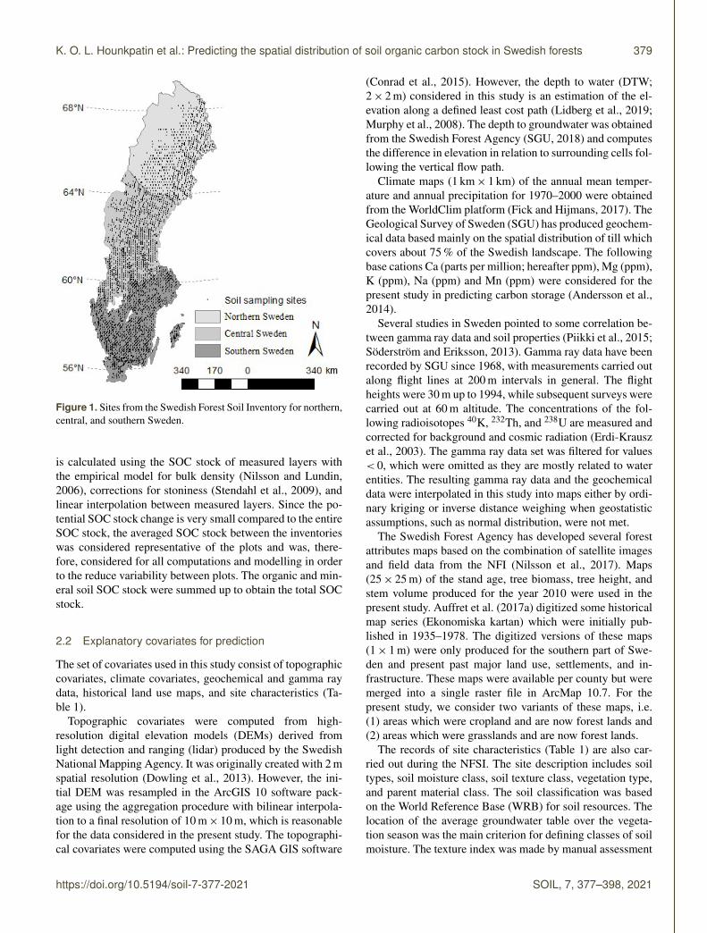
Forest data came from the Swedish National Forest Soil In-ventory (NFSI) and the National Forest Inventory (NFI). TheNFSI runs concurrently every year with the NFI and con-sists of repeated surveys of forest vegetation and soil chem-ical and physical properties (Stendahl et al., 2017; Ortiz etal., 2013). Data from the following inventory periods wereconsidered in the present study: 1993–2002, 2003–2012, and2013–2015. However, the present paper did not focus onSOC changes over these three inventory periods but on SOCstock using plot scale as a unit. The NFSI are conducted onca. 23 500 permanent plots (Fig. 1), with a radius of 10 m,covering all land uses in Sweden except urban areas, culti-vated land, and the high mountains. The plots are distributedbased on a stratified and random national grid system cov-ering all the Swedish forest soils. They are organized inquadratic clusters (tracts) consisting of eight (in the north) tofour (in the southwest) circular (314 m2) sample plots. Eachplot of the NFSI is inventoried once every 10 years.

Soil samples are collected in a subset of the plots, withhumus sampling on ca. 10 000 plots and mineral soil sam-pling on ca. 4500 plots (Stendahl et al., 2017). Based onthe NFSI data set, pedogenetic carbonates are not formed inthese soils due to sufficient leaching and also sedimentarybedrocks, which could potentially contain CaCO3, cover lessthan 1 % of Swedish forests. Therefore, the content of inor-ganic carbon in mineral soil is considered negligible in thestudy area. Humus layer volumetric samples are taken usinga soil core (core diameter 10 cm) below the O horizon downto 30 cm depth. The mineral soil is sampled at 0–10, 10–20, and 55–65 cm depth from the mineral soil surface. Thesesamples are dried at 35 ◦C and sieved to < 2 mm. Total C isdetermined for all samples by dry combustion with elementalanalysers (LECO CNS-1000 and LECO TruMac CN). TotalO horizon SOC stock is calculated from the sampled amountof soil material and the C concentration of the sample. Thetotal mineral SOC stock down to 50 cm depth for each site

SOIL, 7, 377–398, 2021 https://doi.org/10.5194/soil-7-377-2021

K. O. L. Hounkpatin et al.: Predicting the spatial distribution of soil organic carbon stock in Swedish forests 379

Figure 1. Sites from the Swedish Forest Soil Inventory for northern,central, and southern Sweden.

is calculated using the SOC stock of measured layers withthe empirical model for bulk density (Nilsson and Lundin,2006), corrections for stoniness (Stendahl et al., 2009), andlinear interpolation between measured layers. Since the po-tential SOC stock change is very small compared to the entireSOC stock, the averaged SOC stock between the inventorieswas considered representative of the plots and was, there-fore, considered for all computations and modelling in orderto the reduce variability between plots. The organic and min-eral soil SOC stock were summed up to obtain the total SOCstock.

2.2 Explanatory covariates for prediction

The set of covariates used in this study consist of topographiccovariates, climate covariates, geochemical and gamma raydata, historical land use maps, and site characteristics (Ta-ble 1).

Topographic covariates were computed from high-resolution digital elevation models (DEMs) derived fromlight detection and ranging (lidar) produced by the SwedishNational Mapping Agency. It was originally created with 2 mspatial resolution (Dowling et al., 2013). However, the ini-tial DEM was resampled in the ArcGIS 10 software pack-age using the aggregation procedure with bilinear interpola-tion to a final resolution of 10 m× 10 m, which is reasonablefor the data considered in the present study. The topographi-cal covariates were computed using the SAGA GIS software

(Conrad et al., 2015). However, the depth to water (DTW;2× 2 m) considered in this study is an estimation of the el-evation along a defined least cost path (Lidberg et al., 2019;Murphy et al., 2008). The depth to groundwater was obtainedfrom the Swedish Forest Agency (SGU, 2018) and computesthe difference in elevation in relation to surrounding cells fol-lowing the vertical flow path.

Climate maps (1 km× 1 km) of the annual mean temper-ature and annual precipitation for 1970–2000 were obtainedfrom the WorldClim platform (Fick and Hijmans, 2017). TheGeological Survey of Sweden (SGU) has produced geochem-ical data based mainly on the spatial distribution of till whichcovers about 75 % of the Swedish landscape. The followingbase cations Ca (parts per million; hereafter ppm), Mg (ppm),K (ppm), Na (ppm) and Mn (ppm) were considered for thepresent study in predicting carbon storage (Andersson et al.,2014).

Several studies in Sweden pointed to some correlation be-tween gamma ray data and soil properties (Piikki et al., 2015;Söderström and Eriksson, 2013). Gamma ray data have beenrecorded by SGU since 1968, with measurements carried outalong flight lines at 200 m intervals in general. The flightheights were 30 m up to 1994, while subsequent surveys werecarried out at 60 m altitude. The concentrations of the fol-lowing radioisotopes 40K, 232Th, and 238U are measured andcorrected for background and cosmic radiation (Erdi-Krauszet al., 2003). The gamma ray data set was filtered for values< 0, which were omitted as they are mostly related to waterentities. The resulting gamma ray data and the geochemicaldata were interpolated in this study into maps either by ordi-nary kriging or inverse distance weighing when geostatisticassumptions, such as normal distribution, were not met.

The Swedish Forest Agency has developed several forestattributes maps based on the combination of satellite imagesand field data from the NFI (Nilsson et al., 2017). Maps(25× 25 m) of the stand age, tree biomass, tree height, andstem volume produced for the year 2010 were used in thepresent study. Auffret et al. (2017a) digitized some historicalmap series (Ekonomiska kartan) which were initially pub-lished in 1935–1978. The digitized versions of these maps(1× 1 m) were only produced for the southern part of Swe-den and present past major land use, settlements, and in-frastructure. These maps were available per county but weremerged into a single raster file in ArcMap 10.7. For thepresent study, we consider two variants of these maps, i.e.(1) areas which were cropland and are now forest lands and(2) areas which were grasslands and are now forest lands.

The records of site characteristics (Table 1) are also car-ried out during the NFSI. The site description includes soiltypes, soil moisture class, soil texture class, vegetation type,and parent material class. The soil classification was basedon the World Reference Base (WRB) for soil resources. Thelocation of the average groundwater table over the vegeta-tion season was the main criterion for defining classes of soilmoisture. The texture index was made by manual assessment

https://doi.org/10.5194/soil-7-377-2021 SOIL, 7, 377–398, 2021


Table 1. List of explanatory covariates for predicting SOC stock.

Type Variables Abbreviation

Topography Elevation (m) DEMSlope (%) Slopecos(Aspect) cosAspsin(Aspect) sinAspPlan curvature (rad m−1) PLCurProfile curvature (rad m−1) PRCurvTerrain ruggedness index TRISaga wetness index SWIDistance to streams (mm) strDistDepth to water (m) DTWDistance to groundwater (mm) DTG

Climate Temperature (◦C) TempPrecipitation (mm) Prep

Geochemical data Ca, Mg, K,Na, and Mn (ppm)

GeoCa, GeoMg, GeoK,GeoNa, and GeoMn

Gamma ray data 40K (ppm), 232Th (ppm), and 238U (%) GamK, GamTh, and GamU

Forest Stand age (years) For.AgeBiomass (kg) For.BiomHeight (m) For.HeightStem volume (m3) For.Vol

Historical land use Former cropland histCLmap∗ Former grassland histGL

Site characteristics Soil types SoilTyp

Levels 1 – Histosol; 2 – Leptosol; 3 – Gleysol; 4 – Podzol; 5 – Umbrisol; 7 – Arenosol;6 – Cambisol; 8 – Regosol; 9 Unclassified

Soil moisture class SoilMst

Levels 1 – Dry; 2 – fresh; 3 – fresh/moist; 4 – moist; 5 – wet

Soil texture class Texture

Levels 0 – Boulders in the profile; 1 – stone/boulder/bedrock; 2 – gravel/gravelly till;3 – coarse sand/sandy till; 4 – sand/sandy silty till; 5 – fine sand/silty sandy till;6 – coarse silt/coarse silty till; 7 – fine silt/fine silty till; 8 – clay/clayish till/gyttja;9 – peat

Parent material ParMat

Levels 1 – Well-sorted sediments; 2 – poorly sorted sediments; 3 – till; 4 – bedrock; 5 – peat

Vegetation type VegTyp

Levels 1 – tall herbs without shrubs; 2 – tall herbs with shrubs/bilberry; 3 – tall herbwith shrubs/vitis-idaea; 4 – low herbs without shrubs; 5 – low herbs with shrubs/bilberry;6 – low herbs with shrubs/vitis-idaea; 7 – without field layer; – 8 broadleaved grass;9 – narrow-leaved grass; 10 – tall sedge; 11 – low sedge; 12 – horse tail type;13 – bilberry type; 14 – vitis-idaea/whortleberry and marsh rosemary;15 – crowberry/heather type; 16 – poor shrubs type

Coordinates Northern NorthC

Eastern EastC

∗ Used only for the southern part of Sweden.



in the field, e.g. through the rolling and washing test. Thevegetation type, as reported in Table 1, was defined by com-bining the descriptions of the field layers which refer to theunderstorey. Field layers consisted of four main types whichare categorized from fertile to poor, namely herb types (tallor low), grounds without field layer, grass types, and dwarfshrub types.

2.3 Prediction models: random forest and quantileregression forest

The random forest (RF) algorithm was selected for SOCstock prediction. Additionally, the quantile regression forest(QRF) was used to estimate the standard deviation related tothe predictions.

RF is a classification and regression method that buildsmultiple decision trees. For regression, the tree predictorsprovide numerical output instead of class labels for classi-fication (Breiman, 2001). The RF is able to model complexand nonlinear relationships between input predictors and re-sponse covariates. The RF is characterized by double ran-domness in the construction of the decisions trees. An en-semble of growing decision trees is generated by combiningbagging (bootstrap aggregating) along with random featureselection. Bagging consists of producing training data sets(bootstrap sample) by drawing randomly with replacementfrom the original training data set generated. A regressiontree is fitted to each of the bootstrap samples from a randomsubset of the input predictors when deciding to split a node.For any new given input X = x, RF provides the predictionof a single tree as a weighted average of the original obser-vations Yi (i = 1, . . .,n) in each node.

µ (x)=∑n

i=1wi(x,θ )Yi, (1)

where wi is the weight vector which results either in a posi-tive constant when the observation (Yi,Xi) is inherent to theleaf generated from the random vector of covariates or is 0if otherwise. The weight vector (Meinshausen, 2006) wi isdefined as follows:

wi (x,θ )=1{xi ε Rl(x,θ )}

#{j : xj ε Rl(x,θ )

} . (2)

Rl(x,θ ) is the rectangular subspace defined by the leaf l(x,θ )of the tree built from the random vector of covariates θ andthe input xi and xj (j = 1, . . .,n). The conditional meanE(Y |X = x) is computed by averaging the predictions of ksingle trees which are individually built with independentvectors having similar distributions. The weighted averageof trees is computed as follows:

wi (x)= k−1∑k

t=1wi(x,θt ). (3)

The final prediction of the RF regression is given by the fol-lowing:

µ (x)=∑n

i=1wi(x)Yi . (4)

The number of trees to grow in the RF model (ntree) andthe number of randomly selected predictor covariates at eachnode (mtry) are the two key parameters to be tuned for RFmodelling. To reduce computational load, the ntree was setat 500 while the mtry was tuned using the grid search (2– p, with p being the number of covariates) method in theR caret package (Kuhn, 2015) with 50-fold cross validation.The importance of each input predictor can be assessed bythe RF based on the mean decrease accuracy (MDA; Hastieet al., 2011). The MDA is computed by (i) randomly permut-ing the values of each predictor within the out of bag sampleand (ii) measuring the reduction in model accuracy resultingfrom that permutation. The hypothesis is that this permuta-tion would result in little to no effect on model accuracy forless important covariates, while significant drop will followthe permutation of important covariates.

2.4 Covariate layers processing for sub-areas

We considered three sub-areas in Sweden (Fig. 1) which arehereafter reported as northern (north), central (centre), andsouthern (south) Sweden areas in the remainder of the paper.These areas were defined by merging the northern, central,and southern climatic regions which were considered in Ortizet al. (2013). A buffer of 4 km was considered for the shape-files of each sub-area to create overlapping zones which en-sured smooth transition while merging by averaging the SOCstock values within these shared units. The covariates weredelimited for each sub-area. They were resampled to 10 mresolution using the bilinear method for continuous covari-ates and the nearest neighbour method for categorical covari-ates. A value to point extraction was carried out by overlay-ing the coordinates of the sampling points of each sub-areasover the stacked raster files in R (Kuhn, 2015). The pixel val-ues of each sub-area were compiled to form the database ofthe humus layer and mineral and total SOC stock.

2.5 Modelling with different category of covariates:global and local models

For modelling, the following three categories of covariateswere considered: (1) only the plot-level, site-specific covari-ates (SSCs), (2) all the covariates without the SSC, namelythe group of covariates (GoCs), and (3) both the SSCs andGoCs (allCs). Modelling with RF was carried out with eachcategory of covariate related to its sub-areas and for the com-piled data set for the whole of Sweden. Moreover, to reducecomputation time while keeping relatively the same level ofaccuracy, we (1) used feature preprocessing capabilities im-plemented in the caret package (Kuhn, 2019) of R to removehighly correlated (Pearson’s correlation) expressions, using acutoff point of 0.80, and (2) the recursive feature elimination(RFE) using RF as a method to select the optimal set of co-variates for each RF model. The RFE functions by carryingout a variable importance classification then proceeds by it-



eratively eliminating the least important features (Gomes etal., 2019; Hounkpatin et al., 2018). For each RF model, theRFE was carried out, and therefore, the model-specific opti-mal set of covariates were identified for both sub-areas andthe whole of Sweden.

The RF models built on data covering the whole area ofSweden are hereafter called global models. The RF mod-els created for each of the sub-areas are hereafter reportedas local models. Considering the sub-areas as strata, the lo-cal models were built by randomly splitting the local datasets into calibration (80 %) and validation (20 %) subsets (Ta-ble 2). Each local model was validated against their respec-tive local validation set. For comparison, the global modelswere validated using the same local validation set used forthe local models. The data used for calibrating the globalmodel was made up of the 80 % random split of the threelocal training sets (northern, central, and southern trainingsets). The same approach is used for validation at a nationalscale by considering as one data set the 20 % split of the threelocal validation data sets (northern, central, and southern val-idation sets). We trained both global and local models basedon 10-fold cross-validation with five repetitions using the Rcaret package (Kuhn, 2015).

2.6 Assessment of model performance and mapping

To compare model performance, we computed several as-sessment metrics, i.e. R2, Lin’s concordance (Lawrence andLin, 1989) correlation (ρc), root mean square error (RMSE)and mean absolute error (MAE), and the bias.

RMSE=[

1n

∑n

i=1(Pi − Oi)2

]1/2

(5)

R2= 1−

∑ni=1(Pi − Oi)2∑ni=1(Oi − µobs)2 (6)

ρc =2ρσpredσobs

σ 2pred+ σ

2obs+

(µpred− µobs

)2 (7)

MAE=1n

∑n

i=1|Pi −Oi | (8)

Bias= µpred− µobs, (9)

where P is the predicted value, O is the observed/true value,µobs and µpred are the means of the observed and predictedvalues, respectively, σ 2

obs and σ 2pred are the associated vari-

ances, and ρ is the correlation between the observed and thepredicted values.

Though these error metrics are widely used for assess-ing models, they cannot inform about the uncertainty relatedto the prediction. Therefore, we additionally considered thedensity distribution of the predicted versus actual SOC stock.Furthermore, the scattergram of the prediction interval cover-age probability (PICP) was also considered (Vaysse and La-gacherie, 2017). The latter is the graphical representation ofthe proportion of time the actual values of SOC stock fall

Table2.D

escriptivestatistics

forthetraining

andvalidation

datasets.

TrainingV

alidation

nM

inM

axM

edianM

eanSD

Cv

Skewness

nM

inM

axM

edianM

eanSD

Cv

Skewness

Hum

uslayer

North

10080

246.0018.10

23.5721.78

0.924.25

2520

128.0018.05

23.0518.28

0.792.57

(tCha−

1)C

entre1708

0299.52

18.4223.87

21.490.90

3.61424

0143.77

18.4223.54

19.310.82

2.33South

17630

418.8023.05

30.0734.79

1.163.36

4400

418.8023.06

30.5939.75

1.304.42

All

44790

418.8019.52

26.2427.72

1.063.88

11160

418.8019.63

26.2129.18

1.115.07

Mineral

North

4782.36

305.5941.46

46.8525.96

0.553.44

11616.21

136.4741.34

47.7323.07

0.481.35

(tCha−

1)C

entre785

0224.24

48.3153.28

26.460.50

1.60196

0143.14

48.2752.49

23.510.45

0.85South

8750

386.7062.43

68.3240.49

0.591.93

2160

206.0063.09

68.3437.91

0.551.16

All

21380

386.7051.44

58.2233.73

0.582.26

5280

206.0051.81

57.9331.39

0.541.46

TotalN

orth478

16.11360.18

62.9372.46

39.620.55

2.94115

20.02331.56

63.0075.12

45.760.61

2.90(tC

ha−

1)C

entre784

12.88229.87

71.8077.33

31.340.41

1.32196

15.92254.69

71.6978.67

37.200.47

1.78South

8700

487.3789.19

99.3450.63

0.512.37

21616.78

357.2388.99

97.6144.47

0.462.01

All

21320

487.3776.26

85.2243.57

0.512.47

52715.92

357.2376.46

85.6443.32

0.512.11



within a series of probability (p) of prediction intervals (PI)limited by (1−p)/2 and (1+p)/2 quantiles. The QRF wasused to predict all percentiles, including the 5th and 95th per-centile required to create the 90 % prediction intervals. Fi-nally, the coverage of the 90 % prediction intervals by theobservation from the validation set was also analysed.

The SOC stock maps were computed only for the mod-els based on the GoC models because of their availability asmaps. The uncertainty in the SOC stock predictions was ex-pressed by considering the coefficient of variation which isthe percentage ratio of the standard deviation map dividedby the mean SOC stock prediction. A qualitative assessmentof the spatial distribution of the humus layer, mineral soil,and total SOC stock from the produced maps was carried outand compared to literature.

3 Results

3.1 Validation performance of global models over thewhole of Sweden

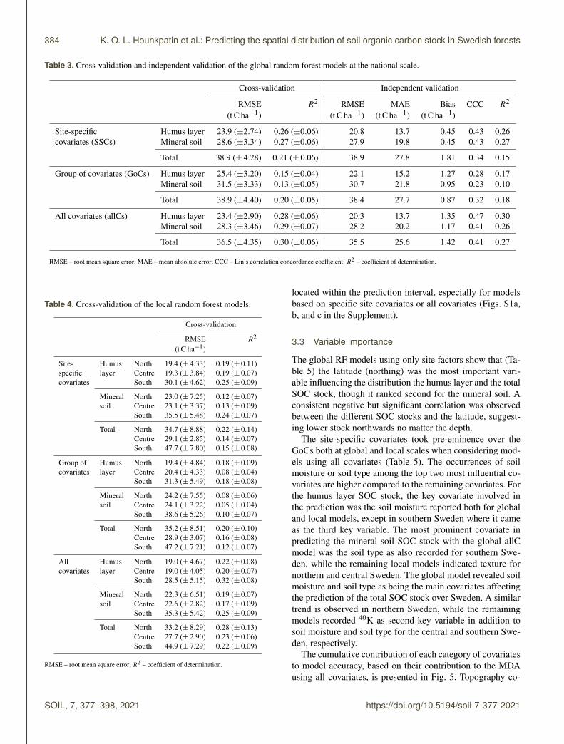
The performance metrics of the cross- and independent vali-dation of the RF models at the national scale are presented inTable 3. The internal accuracy statistics showed that mod-elling with all covariates generally resulted in marginallylower RMSE and higher R2 for all SOC stock. Modellingwith allCs reduced the cross-validation RMSE by 2 %, 1 %,and 6 % compared to SSC models and by 7.9 %, 10 %, and6 % compared to GoC models, respectively, for the humuslayer, mineral soil, and total SOC stock. Though modellingwith allCs resulted in higher cross-validation R2 comparedto the remaining models, only 30 %, 29 %, and 28 % of thetotal variance were explained, respectively, for the total SOCstock, mineral soil, and the humus layer SOC stock.

The independent validation showed similar trends as ob-served for the cross-validation. The Lin’s correlation concor-dance coefficient (CCC) confirmed that the predictive per-formance of RF for the different SOC stock was enhancedeither by using only SSCs or allCs. The similarity betweenthe RMSE values of both training and validation data showsthat the global models over Sweden did no overfit. However,the explained variances are as low as for the cross-validationvarying from 15 % to 27 % for the SSC models, 10 % to 18 %for the GoC models, and from 26 % to 30 % for the allC mod-els. For both cross- and independent validation, the RMSEincreased with depth, with the lowest values recorded for thehumus layer.

3.2 Validation performance of local models versusglobal models

As observed for the global models at the national scale, bet-ter accuracy was recorded for the local models based onallCs and SSCs, which present, in general, lower RMSE andhigher CCC and R2 when compared to the local GoC mod-

els for the cross-validation (Table 4). The cross-validationwith the local models resulted in lower RMSE compared tothe values recorded for the global models (Table 3), exceptfor the southern Sweden models which recorded higher val-ues regardless of the category of covariates. Local modelswith allC reduced the RMSE of cross-validation in relationto the global models (Table 3) by 18 % for both northernand central Sweden for the humus layer SOC stock, by 21 %(north) and 20 % (centre) for the mineral soil SOC stock, andby 9 % (north) and 24 % (central) for the total SOC stock.The variances explained by the local models based on cross-validation varied from 17 % to 32 % for allC models, 12 % to25 % for the SSC models, and from 5 % to 20 % for the GoCmodels.

The global models were also used to make predictionswith the same independent validation set used for the lo-cal models. Though the local models generally outperformedthe global models, the results were different based on thesub-areas and category of covariates (Fig. 2). However, thelocal SSC models were more consistent at outperformingthe global SSC models compared to GoC and allC modelswhen tested with an independent data set. For the humuslayer (Fig. 2a) and the mineral (Fig. 2b) and total soil lay-ers (Fig. 2c), the local models had, in general, better perfor-mance than the global models in term of RMSE within eachset of variables. The best local models were mostly associ-ated with all covariates or site-specific covariates, especiallyfor central and southern Sweden. It was only with the localmodel of mineral SOC stock for northern Sweden that theGoC gave a better accuracy compared to other models. It wasalso noted that the RMSE of the local models increased ingeneral from the humus layer to the mineral soil for both thecross- and independent validation, as previously observed forthe global models, no matter the validation type and categoryof factors.

The local and global models showed similar trend for thedensity distribution of actual versus predicted SOC stock(Fig. 3). For Figs. 3 and 4, only global and local models withthe lowest RMSE were reported to avoid redundancies. AllRF models presented an underestimation of lower and highervalues of SOC stock, while an overestimation was observedfor the values centred around the means. However, underes-timation of high values was less pronounced with the globalmodels over the entire Sweden and also with the predictionsfor the humus layer. The local model associated with thegroup of covariates of the mineral soil SOC stock in northernSweden also presented a pronounced overestimation of thelower values.

The PICP estimates seem to correspond quite well withthe respective confidence level (Fig. 4), except for the humusand mineral SOC stock of southern Sweden. For southernSweden, it appears that at a higher level of confidence thecorresponding PICP is higher for the humus layer and lowerfor the mineral SOC stock. Considering a 90 % prediction in-terval, most of the validation observations (80 %–95 %) were



Table 3. Cross-validation and independent validation of the global random forest models at the national scale.

Cross-validation Independent validation

RMSE R2 RMSE MAE Bias CCC R2

(t C ha−1) (t C ha−1) (t C ha−1) (t C ha−1)

Site-specific Humus layer 23.9 (±2.74) 0.26 (±0.06) 20.8 13.7 0.45 0.43 0.26covariates (SSCs) Mineral soil 28.6 (±3.34) 0.27 (±0.06) 27.9 19.8 0.45 0.43 0.27

Total 38.9 (± 4.28) 0.21 (± 0.06) 38.9 27.8 1.81 0.34 0.15

Group of covariates (GoCs) Humus layer 25.4 (±3.20) 0.15 (±0.04) 22.1 15.2 1.27 0.28 0.17Mineral soil 31.5 (±3.33) 0.13 (±0.05) 30.7 21.8 0.95 0.23 0.10

Total 38.9 (±4.40) 0.20 (±0.05) 38.4 27.7 0.87 0.32 0.18

All covariates (allCs) Humus layer 23.4 (±2.90) 0.28 (±0.06) 20.3 13.7 1.35 0.47 0.30Mineral soil 28.3 (±3.46) 0.29 (±0.07) 28.2 20.2 1.17 0.41 0.26

Total 36.5 (±4.35) 0.30 (±0.06) 35.5 25.6 1.42 0.41 0.27

RMSE – root mean square error; MAE – mean absolute error; CCC – Lin’s correlation concordance coefficient; R2 – coefficient of determination.

Table 4. Cross-validation of the local random forest models.

Cross-validation

RMSE R2

(t C ha−1)

Site- Humus North 19.4 (± 4.33) 0.19 (± 0.11)specific layer Centre 19.3 (± 3.84) 0.19 (± 0.07)covariates South 30.1 (± 4.62) 0.25 (± 0.09)

Mineral North 23.0 (± 7.25) 0.12 (± 0.07)soil Centre 23.1 (± 3.37) 0.13 (± 0.09)

South 35.5 (± 5.48) 0.24 (± 0.07)

Total North 34.7 (± 8.88) 0.22 (± 0.14)Centre 29.1 (± 2.85) 0.14 (± 0.07)South 47.7 (± 7.80) 0.15 (± 0.08)

Group of Humus North 19.4 (± 4.84) 0.18 (± 0.09)covariates layer Centre 20.4 (± 4.33) 0.08 (± 0.04)

South 31.3 (± 5.49) 0.18 (± 0.08)


South 38.6 (± 5.26) 0.10 (± 0.07)


All Humus North 19.0 (± 4.67) 0.22 (± 0.08)covariates layer Centre 19.0 (± 4.05) 0.20 (± 0.07)

South 28.5 (± 5.15) 0.32 (± 0.08)


South 35.3 (± 5.42) 0.25 (± 0.09)


RMSE – root mean square error; R2 – coefficient of determination.

located within the prediction interval, especially for modelsbased on specific site covariates or all covariates (Figs. S1a,b, and c in the Supplement).

3.3 Variable importance

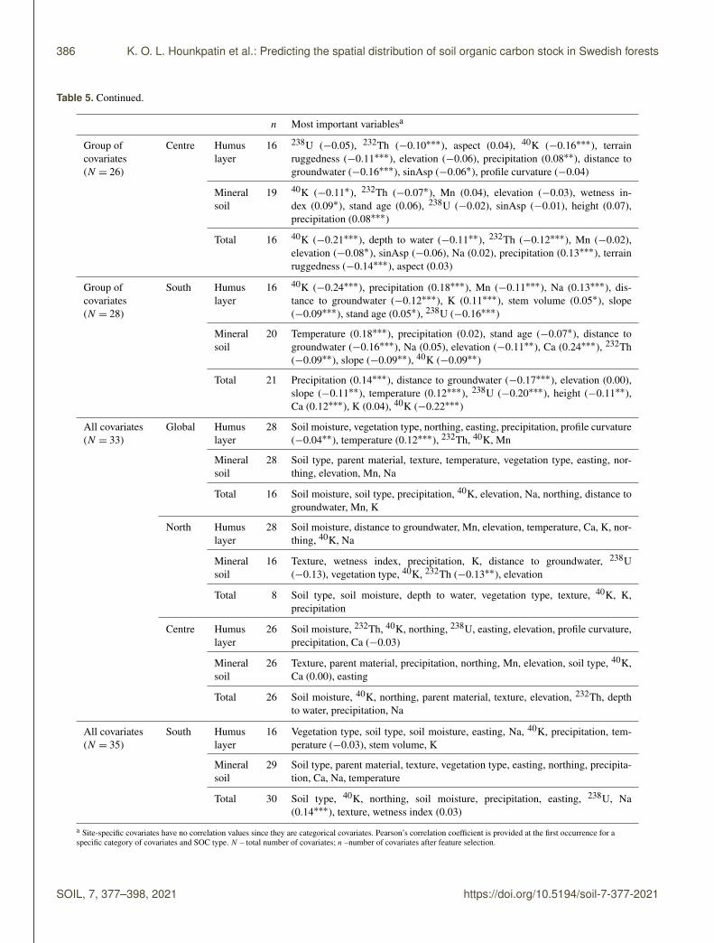
The global RF models using only site factors show that (Ta-ble 5) the latitude (northing) was the most important vari-able influencing the distribution the humus layer and the totalSOC stock, though it ranked second for the mineral soil. Aconsistent negative but significant correlation was observedbetween the different SOC stocks and the latitude, suggest-ing lower stock northwards no matter the depth.

The site-specific covariates took pre-eminence over theGoCs both at global and local scales when considering mod-els using all covariates (Table 5). The occurrences of soilmoisture or soil type among the top two most influential co-variates are higher compared to the remaining covariates. Forthe humus layer SOC stock, the key covariate involved inthe prediction was the soil moisture reported both for globaland local models, except in southern Sweden where it cameas the third key variable. The most prominent covariate inpredicting the mineral soil SOC stock with the global allCmodel was the soil type as also recorded for southern Swe-den, while the remaining local models indicated texture fornorthern and central Sweden. The global model revealed soilmoisture and soil type as being the main covariates affectingthe prediction of the total SOC stock over Sweden. A similartrend is observed in northern Sweden, while the remainingmodels recorded 40K as second key variable in addition tosoil moisture and soil type for the central and southern Swe-den, respectively.

The cumulative contribution of each category of covariatesto model accuracy, based on their contribution to the MDAusing all covariates, is presented in Fig. 5. Topography co-



Table 5. Random forest variable importance for the global and local models for the humus layer, mineral soil, and total SOC stock withtheir associated Pearson’s coefficient of correlation with the covariates (values in parenthesis are as follows: ∗ p ≤ 0.05; ∗∗ p ≤ 0.01;∗∗∗ p ≤ 0.001).

n Most important variablesa

Site-specificcovariates

Global Humuslayer

7 Northing (−0.12∗∗∗), soil moisture, easting (−0.09∗∗∗), vegetation type, soiltype, parent material, texture

(N = 7) Mineralsoil

7 Easting (−0.13∗∗∗), northing (−0.27∗∗∗), soil type, vegetation type, texture,parent material, soil moisture

Total 7 Northing (−0.28∗∗∗), soil moisture, soil type, easting (−0.15∗∗∗), texture, veg-etation type, parent material

North Humuslayer

7 Soil moisture, soil type, vegetation type, northing (−0.09∗∗), easting (0.06),parent material, texture

Mineralsoil

7 Easting (−0.13∗∗), vegetation type, texture, parent material, northing (−0.09∗),soil moisture, soil type

Total 7 Soil moisture, soil type, vegetation type, texture, parent material, easting (0.00),northing (−0.11∗)

Centre Humuslayer

4 Soil moisture, northing (−0.08∗∗∗), easting (−0.02), vegetation type

Mineralsoil

4 Parent material, texture, northing (−0.05), soil type, soil moisture, easting(0.00)

Total 7 Soil moisture, northing (−0.13∗∗∗), easting (0.03), parent material, texture, veg-etation type, soil type

South Humuslayer

4 Vegetation type, soil moisture, soil type, easting (−0.15∗∗∗)

Mineralsoil

7 Soil type, easting (0.02), northing (−0.08∗), vegetation type, parent material,texture, soil moisture

Total 4 Soil type, easting (−0.10∗∗), soil moisture, northing (−0.13∗∗∗)

Group ofcovariates(N = 26)

Global Humuslayer

20 Mn (−0.08∗∗∗), precipitation (0.16∗∗∗), 40K (−0.20∗∗∗), 232Th (−0.15∗∗∗),Na (0.03), terrain ruggedness (−0.11∗∗∗), K (−0.07∗∗∗), distance to ground-water (−0.14∗∗∗), 238U (−0.10∗∗∗), sinAsp (−0.06∗∗∗)

Mineralsoil

20 Temperature (0.28∗∗∗), precipitation (0.18∗∗∗), Mn (0.05∗∗), elevation(−0.16∗∗∗), terrain ruggedness (−0.12∗∗∗), Na (−0.05), Ca (0.22∗∗∗), 40K(−0.13∗∗∗), wetness index (0.11∗∗∗), K (0.01)

Total 21 Temperature (0.28∗∗∗), distance to groundwater (−0.17∗∗∗), precipitation(0.21∗∗∗), 40k (−0.24∗∗∗), 232th (0.16∗∗∗), Na (−0.01), K (−0.04), Mn(−0.02), 238U (−0.11∗∗∗), elevation (−0.18∗∗∗)

North Humuslayer

8 40K (−0.23∗∗∗), distance to groundwater (−0.18∗∗∗), elevation (−0.15∗∗∗), Ca(−0.06), temperature (0.16∗∗∗), Mn (−0.10∗∗), Na (−0.06), K (0.00)

Mineralsoil

8 40K (−0.25∗∗∗), wetness index (−0.01), Ca (−0.05), Na (−0.09), temperature(0.01), precipitation (0.16∗∗∗), K (0.04), aspect (0.03), stand age (0.02), eleva-tion (0.13∗)

Total 8 Depth to water (−0.22∗∗∗), 40K (−0.30∗∗∗), K (0.04), temperature (0.10∗),precipitation (0.16∗∗∗), elevation (−0.06), Mn (−0.07), distance to streams(−0.15∗∗∗)



Table 5. Continued.

n Most important variablesa


Centre Humuslayer

16 238U (−0.05), 232Th (−0.10∗∗∗), aspect (0.04), 40K (−0.16∗∗∗), terrainruggedness (−0.11∗∗∗), elevation (−0.06), precipitation (0.08∗∗), distance togroundwater (−0.16∗∗∗), sinAsp (−0.06∗), profile curvature (−0.04)

Mineralsoil

19 40K (−0.11∗), 232Th (−0.07∗), Mn (0.04), elevation (−0.03), wetness in-dex (0.09∗), stand age (0.06), 238U (−0.02), sinAsp (−0.01), height (0.07),precipitation (0.08∗∗∗)

Total 16 40K (−0.21∗∗∗), depth to water (−0.11∗∗), 232Th (−0.12∗∗∗), Mn (−0.02),elevation (−0.08∗), sinAsp (−0.06), Na (0.02), precipitation (0.13∗∗∗), terrainruggedness (−0.14∗∗∗), aspect (0.03)


South Humuslayer

16 40K (−0.24∗∗∗), precipitation (0.18∗∗∗), Mn (−0.11∗∗∗), Na (0.13∗∗∗), dis-tance to groundwater (−0.12∗∗∗), K (0.11∗∗∗), stem volume (0.05∗), slope(−0.09∗∗∗), stand age (0.05∗), 238U (−0.16∗∗∗)

Mineralsoil

20 Temperature (0.18∗∗∗), precipitation (0.02), stand age (−0.07∗), distance togroundwater (−0.16∗∗∗), Na (0.05), elevation (−0.11∗∗), Ca (0.24∗∗∗), 232Th(−0.09∗∗), slope (−0.09∗∗), 40K (−0.09∗∗)

Total 21 Precipitation (0.14∗∗∗), distance to groundwater (−0.17∗∗∗), elevation (0.00),slope (−0.11∗∗), temperature (0.12∗∗∗), 238U (−0.20∗∗∗), height (−0.11∗∗),Ca (0.12∗∗∗), K (0.04), 40K (−0.22∗∗∗)

All covariates(N = 33)

Global Humuslayer

28 Soil moisture, vegetation type, northing, easting, precipitation, profile curvature(−0.04∗∗), temperature (0.12∗∗∗), 232Th, 40K, Mn

Mineralsoil

28 Soil type, parent material, texture, temperature, vegetation type, easting, nor-thing, elevation, Mn, Na

Total 16 Soil moisture, soil type, precipitation, 40K, elevation, Na, northing, distance togroundwater, Mn, K

North Humuslayer

28 Soil moisture, distance to groundwater, Mn, elevation, temperature, Ca, K, nor-thing, 40K, Na

Mineralsoil

16 Texture, wetness index, precipitation, K, distance to groundwater, 238U(−0.13), vegetation type, 40K, 232Th (−0.13∗∗), elevation

Total 8 Soil type, soil moisture, depth to water, vegetation type, texture, 40K, K,precipitation

Centre Humuslayer

26 Soil moisture, 232Th, 40K, northing, 238U, easting, elevation, profile curvature,precipitation, Ca (−0.03)

Mineralsoil

26 Texture, parent material, precipitation, northing, Mn, elevation, soil type, 40K,Ca (0.00), easting

Total 26 Soil moisture, 40K, northing, parent material, texture, elevation, 232Th, depthto water, precipitation, Na

All covariates(N = 35)

South Humuslayer

16 Vegetation type, soil type, soil moisture, easting, Na, 40K, precipitation, tem-perature (−0.03), stem volume, K

Mineralsoil

29 Soil type, parent material, texture, vegetation type, easting, northing, precipita-tion, Ca, Na, temperature

Total 30 Soil type, 40K, northing, soil moisture, precipitation, easting, 238U, Na(0.14∗∗∗), texture, wetness index (0.03)

a Site-specific covariates have no correlation values since they are categorical covariates. Pearson’s correlation coefficient is provided at the first occurrence for aspecific category of covariates and SOC type. N – total number of covariates; n –number of covariates after feature selection.



Figure 2. Local and global models ranked by decreasing RMSE per sub-area and category of variables along with correspondingR2 (a – litterlayer; b – mineral soil layer; c – total soil layer; SSCs – site-specific covariates; GoCs – group of covariates; allCs – all covariates).

variates greatly influence model accuracy in the northern partof Sweden, contributing to about 30 %–40 % of the modelMDA, especially for the humus layer and mineral soil SOCstock. This is further corroborated by a high correlation ofthese covariates with the SOC stock in northern Sweden (Ta-ble 5). For the humus and mineral SOC stock, the importance

of topography decreased from the north to the south of Swe-den with the gamma ray, site-specific, and climate covariatesgaining more prominence (contributing together up to 60 %of MDA) in central Sweden, while site factors were the mostinfluential variable with a share of 40 % of MDA in south-ern Sweden (Fig. 5). These categories of covariates, which



Figure 3. Density plots of the actual versus predicted humus layer, mineral soil, and total SOC stock from the local and global random forestmodels (with lowest root mean square errors). Line – average values; SSCs – site-specific covariates; GoCs – group of covariates; allCs – allcovariates; dashed lines – mean of SOC stock.

ranked first in central and southern Sweden, were also classi-fied among the top three covariates – site-specific covariates,climate, and gamma ray data – for the global humus layermodel.

As observed for the humus layer, topography was lessprominent for central and southern Sweden for both mineralsoil and total SOC stock (Fig. 5). Site-specific covariates, cli-mate, and geochemical data, which provided the highest con-tribution to MDA mineral soil for the global model over Swe-den, were also the most influential over central and southernSweden, contributing together up to 60 % and 70 % to theMDA. Gamma ray data seemed to play a key role in the dis-tribution of the total SOC stock, especially in southern Swe-den, together with the site-specific covariates and climate. Itis important to note that, for the global model of the totalSOC layer, the different category of covariates contributedalmost equally to the MDA, with the gamma ray and climatetaking pre-eminence over the site-specific covariates. Theforest covariates had very low contributions as compared tothe remaining (Fig. 5) category of covariates, and they weremostly absent from the top 10 (Table 5), while those rankedhave very low correlation with the different SOC stock.

3.4 Maps of SOC stock

Figure 6 shows the SOC stock maps from the GoC globaland local models. Though the global GoC models generallyoutperformed the local GoC models (Table 4), their predic-

tive maps generally follow the same pattern. Broadly, thereis an increasing gradient of SOC stock from north to southfor the humus layer, mineral soil, and total SOC stock. Thelocal models tend to present lower values of SOC stock innorthern and central Sweden for the humus layer, while theglobal model displays higher values over the whole country.For the mineral soil, there seems to be no distinct differencein the spatial prediction of SOC stock, which resulted in asimilar pattern from the north to the south for both local andglobal model maps. Since the total SOC stock is the sumbetween the humus layer and mineral SOC stock, its spa-tial distribution follows the same trend, with the lowest SOCrecorded in northern and central Sweden while higher stockare located in the south. No matter the type of SOC stock,the coefficient of variation is high and generally above 60 %throughout Sweden.

4 Discussion

4.1 Prediction with global and local models

This study examined how global and local models differ inpredicting the humus layer, mineral soil, and total SOC stockin Swedish forests. The local models recorded lower RMSEat the modelling stage with the cross-validation compared tothe global models, except for the southern area. When pre-dictions were carried out on the same validation set, localmodels, including those of southern Sweden, generally out-performed the global models. This suggests, on the one hand,



Figure 4. Prediction interval coverage probability of the local and global random models for the humus layer, mineral soil, and total SOCstock. SSCs – site-specific covariates; GoCs – group of covariates; allCs – all covariates.

Figure 5. Variable importance of the main category of covariates for local and global random models for the humus layer, mineral soil, andtotal SOC stock.



Figure 6. Mean SOC stock prediction and prediction uncertainties of the spatial distribution of the humus layer, mineral soil, and total SOCstock based on the group of covariates.

that global models with higher sample size might not neces-sarily result in a more accurate model compared to modelsbuilt from a reduced data set corresponding to a sub-areaof a bigger region. On the other hand, the particular casefor southern Sweden suggests that, though a global modelmight present a comparative advantage at modelling stage,

it might not necessarily have a better predictive power whenconfronted with a new set of samples. The findings of thisstudy are in line with those of Somarathna et al. (2016), whoalso found locally calibrated models to perform better thanglobal models for predicting SOC content. However, the re-sults of the present study differed from the latter in that the



comparative advantage was dependent of the category of co-variates used.

Findings (Fig. 2) showed that local models which outper-formed global models were either associated with all covari-ates or site-specific covariates. For example, local models incentral Sweden required all covariates to outperform globalmodels for the humus layer, mineral soil, and total SOCstock. The same pattern was observed for southern Sweden,except for the mineral SOC stock for which the best localmodel was associated with the SSCs. The local best modelfor the total SOC stock in northern Sweden was also associ-ated with SSCs. The higher occurrences of SSCs and allCswith the best local models showed that modelling with GoCsalone is not the optimal choice. On the one hand, forest SSCsare more relevant for capturing the local variability in thesampling plots than the other covariates which are mostly re-mote sensing products. When both SSCs and GoCs are usedas covariates, the locally specific information at plot scaleare complemented by higher-scale covariates which cover alarger range of the feature space, resulting in model improve-ment, especially for the humus layer.

In addition, using both site characteristics and remotelysensed products for predicting SOC stock generally in-creased the variance explained with both cross-validation andindependent validation methods for the humus layer, min-eral soil, and total SOC stock. However, despite the combi-nation of these two categories of covariates, the accuracy ofthe SOC stock prediction remained low for both the globalmodels (maximum R2 is 0.30) and local models (maximumR2 is 0.33). There seems to be no study comparable in scopeand methodology targeting the prediction of SOC stock inforest soils. The closest is the digital mapping of SOC stockfor the humus layer and mineral stock using machine learn-ing models such as RF and the k nearest neighbour (kNN)based on data set from the national forest inventory of theUSA (Cao et al., 2019). The authors also found a lower fitbetween predicted and observed SOC stock after the inde-pendent validation and reported an R2 of 0.20 and 0.11 forthe humus layer, while recording an R2 of 0.33 and 0.28 forthe mineral soil, respectively, for the RF and kNN models.Other studies conducted in temperate forests for predictingSOC stock also showed poor goodness of fit values, with across-validation R2 of 0.22 (1 m depth) with the boosted re-gression trees (Ottoy et al., 2017). For other soil properties,Mansuy et al. (2014) reported, for some Canadian managedforest, an R2 of 0.04 and 0.05 for SOC content in the humuslayer and mineral soil, respectively, with the kNN, while Be-guin et al. (2017) recorded, for the Canadian forest, an R2 of0.05 for SOC content for the mineral soil with RF model.

Low explained variances in predictive modelling could berelated to different factors (Nelson et al., 2011). For exam-ple, the omission of key covariates with greater explanatorypower or conversely using non-essential covariates with verylow explanatory power which only increase the predictionerror variance. Omitting key covariates in relation to SOC

stock for forest ecosystem in the present study is less likelysince covariates considered in this study well represent thesurrogates for soil forming factors considered in the Soils,Climate, Organisms, Parent material, Age and (N) space orspatial position (SCORPAN) equation defined by McBratneyet al. (2003). In addition, the removal of redundant and non-informative covariates was carried out via dimension reduc-tion, with the exclusion of highly correlated covariates andelimination of some others via recursive feature elimination.However, the Pearson correlations (min= 0; max= 0.28) be-tween covariates and the different SOC stock were found tobe poor though significant for most of the predictors (Table 5;Figs. S2–S4). This could be expected because the data covera wide range of different site conditions, soil types, and par-ent materials.

Another source of the errors could be inherent to themodel, with prediction accuracy varying with different typeof model. Many studies have already compared different ma-chine learning models and concluded that RF generally hasa strong predictive ability in different ecosystems (Cao et al.,2019; Forkuor et al., 2017; Wang et al., 2018). Preliminarysteps in the present study also tested extreme gradient boost-ing and Cubist models (results not shown) alongside the RF,with the latter displaying higher predictive capabilities. Onthe other hand, applying geostatistical approaches (Fig. S5)for the humus layer, mineral soil, and total SOC stock re-vealed very low spatial autocorrelation for the different SOCstock, suggesting that the structure of the SOC data has ashorter range than the sampling interval. For soil propertieswhich vary over short distance, such as SOC stock, data-driven models such as RF might capture the inherent variabil-ity better when modelling data are a good representative ofthe phenomenon that the SOC stock is subject to in the land-scape, including small-scale variation. Beguin et al. (2017)recorded poor performance of different models, includingRF, for predicting C : N because the sampling scheme failedto capture the distance variation (< 20 km) at which a betteraccuracy would have occurred. Model accuracy would likelyimprove if more samples covering the spatial variability ineach inventory plot were taken. The increase in RMSE withdepth recorded for some models is consistent with previousstudies, where the prediction of lower soil layers resulted inlower accuracy (Henderson et al., 2005; Yam et al., 2019).This may be due to a higher sensitivity of the humus layerwhich is directly exposed to the influence of environmentalcovariates.

The estimates of SOC stocks are slightly biased towardsthe extreme values, with an underestimation of the lowestand highest values for both local and global models (Fig. 3).This tends to confirm earlier findings which reported issuesrelated to the underestimation or overestimation of extremevalues by the RF model (Ceh et al., 2018; Hu et al., 2020;Horning, 2010). On the one hand, this seems to be typicalfor regression models with RF because predictions are theaverage values of all of the trees, with a tendency to predict



the mean when the correlation of response and covariate isweak. On the other hand, this may also be related to an under-representation of the lower and higher values compared tothose centred around the mean in the training data set. How-ever, though underestimation of the lowest and highest val-ues could be recorded for all models, the 90 % PICP shows,in general, that the 90 % prediction interval adequately cov-ers the observed values of the humus, mineral, and total SOCstock layers (Fig. 4). This is an indication that the predictionintervals are accurate representative of the prediction uncer-tainties for each of these SOC stocks for both local and globalmodels. However, for southern Sweden, the PICP presentedhigher values for the humus layer and lower values for themineral SOC stock with increasing level of confidence, sug-gesting a higher level of uncertainties in the predictions. Thiscould be attributed to southern Sweden being characterizedby a longer management history and more intensive forestrycompared to northern Sweden (Angelstam and Pettersson,1997), leading to a diversity in forest management patternswith potential feedback on SOC stock distribution.

4.2 Variable importance and modelling accuracy

SOC stocks in forest soils are the product of the dynamicequilibrium between the input flux of plant-derived materi-als and output flux of carbon as a result of decomposition.Classical soil-forming factors – climate, organisms (vegeta-tion, fauna, and human activities), topography, parent mate-rial, and time – are known to govern the amount and distribu-tion of SOC stock. Though covariates used as proxy for thesesoil-forming factors were considered separately for the sakeof analysis in this study, they are actually involved in dy-namic interactions leading to complex soil processes in thelandscape.

With the global RF models using only site-specific covari-ates, the latitude (northing) was the main variable driving thedistribution of the SOC stock, with a negative correlationsuggesting lower stock to the north (Table 5). The latitudi-nal gradient (Millberg et al., 2015) in Sweden also resultsin climatic gradient (Jungqvist et al., 2014), which, in turn,interacts with topography (Johansson and Chen, 2003) to de-termine the heterogeneity in net primary production in rela-tion to the spatial variability in precipitation and temperature.Even at a regional level, the latitude was still critical and wasmostly present among the top 10 covariates being selectedby the local RF models using all covariates (Table 5). How-ever, climate and topographical covariates were consistentlyovershadowed by SSCs when all the covariates were used formodelling both at a national and regional scale. Though pre-cipitation regulates net primary productivity (NPP) and tem-perature controls microbial decomposition of organic mat-ter, their local variability is generally small (Wiesmeier etal., 2019). This makes them less relevant in contrast to SSCstaken at plot level, which describe more closely the factors

controlling the decomposition and stabilization of organicmatter.

Among the site characteristics, the soil moisture was thekey site factor affecting the humus layer SOC stock, es-pecially in the northern and central Sweden, while vegeta-tion type was ranked first in southern part of Sweden (Ta-ble 5). The box plots of these two covariates showed thatthey clearly have different distributions of SOC stock in thehumus layer, although some of the interquartile ranges over-lap (Fig. S6). As observed for the humus layer, soil moisturewas the most important variable associated with total SOCstock along with the soil type. For a sequence from dry tomoist soils, there was an increase in SOC stock in the hu-mus layer and for the mineral and total stock (box plot ofsoil moisture in Figs. S6–S8). This might be explained byhigher productivity in litter supply as water is more availablein the tree root zone of fresh and moist sites. On the otherhand, these latter soils are subject to a longer period of satu-ration (reducing conditions) that slows down decomposition.The impact of soil moisture could also be noted when con-sidering the partial dependence plot of the RF global modelof the humus layer showing the interaction between the soilmoisture class and vegetation type (Fig. S9a). Each vegeta-tion type consistently tends towards higher values of SOCstock for moist sites compared to dry and fresh sites.

Generally, soil type and texture were ranked by the allCglobal models as being the top covariates influencing theSOC stock in the mineral soil (Table 5). The link betweenthese two covariates could be related to the soil moisturecontent of their classes. On the one hand, soil types (His-tosols and Gleysols) with fine texture (fine silt and clay) andhigh moisture content are more subject to reducing condi-tions with higher SOC stock compared to soils (Leptosolsand Arenosols) with a coarse (stone, boulder, and coarsesand) texture. On the other hand, the relevance of soil tex-ture as a predictor of SOC could be related to the physico-chemical SOC stabilization mechanisms. Clay minerals andclay- and silt-sized particles generally have a positive corre-lation with mineral SOC stocks, as the association of organicmatter with mineral surfaces and occlusion inside aggregateshinders microbial decomposition and enhances SOC accu-mulation (Lützow et al., 2006; Zhang et al., 2020).

The addition of the other group of covariates (GoCs) tothe site-specific covariates resulted in limited improvementfor both global and local models (Tables 3–4). This sug-gests that their level of distinct complementarity in the fea-ture space is low as the GoCs might be carrying redundantinformation with the site-specific covariates in relation to thehumus layer, mineral soil, and total stock. For example, theprominence of site-specific covariates over topographical co-variates (Table 5; allCs) might be due to the fact they are in-directly incorporated into the definition of the site-specificcovariates. For this study, wetness index, distance to ground-water, and depth to water are indexes used to characterize soilmoisture, while gamma ray data describe parent material. A



similar observation was shared by Wiesmeier et al. (2011)who, also recorded land use and soil type as being key co-variates affecting SOC stock, while topographic covariatescontributed very weakly to model accuracy using randomforest. However, though ranked low among all covariates(Table 5; allCs), the cumulated variable importance analysisshowed that topographical covariates stood out in contribut-ing to model accuracy in northern Sweden (Fig. 5) but wereless relevant in the south. Obviously, higher elevation andderivatives in northern Sweden explain such an influence onthe SOC stock.

Next to site characteristics and climate, the cumulativegamma ray data were more consistent in contributing tomodel accuracy of the total SOC stock compared to geo-chemical data, with the individual ranking further reveal-ing a higher occurrence of radioactive K both at the globaland regional level (Table 5; Fig. 5). This suggests that K-bearing minerals of the parent material have greater explana-tory power over total SOC stock than U and Th, the nature ofwhich might require further studies. Malone et al. (2009) alsorecorded gamma K as being the key covariate for mappingSOC stock in an agriculture dominated land use in Australia.

The geochemical data were revealed to be the key covari-ates in the distribution of SOC stock in southern Sweden,especially for the humus layer (Na) and mineral stock (Caand Na), though of a much lower magnitude compared tosite-specific covariates. However, base cations seemed not toprimarily affect SOC distribution but rather environmentalcovariates that regulate their dynamics. The low ranking offorest parameters may be related to (1) their low correlationswith the SOC stock data and (2) the fact that the data set cutacross different data forest types without any specific strati-fication, which could have created a homogeneous strata formodelling. However, the focus of the present study was noton a specific forest type, which could have further reducedthe training data set, while machine learning models requirehigh data samples to learn patterns and accurately predict tar-get values on independent data sets.

4.3 Spatial prediction of SOC stock

The maps of the humus layer, mineral soil, and total stockpresent a pattern of the increasing accumulation of SOCstocks from south to north, with the highest uncertaintiesin the southern part of Sweden regardless of the predictingmodels (Fig. 6). In general, it is expected that the global lat-itudinal trend will result in increasing stocks in higher lati-tudes, which correspond to colder and humid regions. Pos-sible explanations are associated with slower microbial de-composition rates, while other studies suggest non-conducivesoil conditions such as water logging, low pH values, andhigh aluminium concentration as being the main constraints(Dieleman et al., 2013; Hobbie et al., 2000; Wiesmeier et al.,2019).

The contrary configuration observed in the maps, with adecreasing south–north distribution in the SOC stock for thehumus layer and mineral soil (Fig. S10), is consistent withfindings from different studies (Kleja et al., 2008; Fröberget al., 2011; Hyvonen et al., 2008). These studies advocatethat the high SOC stocks in the south could be related to ahigher deposition of nitrogen (N) compared to central andnorthern Sweden. It has been suggested that N deposition re-sults in both increasing litter inputs and increasing mean res-idence time. Also, high concentrations of inorganic N inhibitthe activities of lignin-degrading phenol oxidase released bymicroorganisms (Zak, 2017; Carreiro et al., 2000). How-ever, a warmer climate makes trees grow faster, along with ahigher litter input, in the south than in the north. With the co-occurring north–south gradient of temperature (lower), pH(higher), soil carbon (lower; Iwald, 2016; Framstad, 2013),and N deposition might have contributed to the strengtheningof the north–south SOC stock gradient. As southern Sweden(Fig. 6) recorded a higher range in SOC stocks, the associ-ated average variation around the mean was also larger.

4.4 Implication and limitations of the study

The present study compared a local and a global modellingapproach for DSM. To the question of which approach touse when mapping a big area, our research showed that itis dependent on the type of covariates available. In general,building local models for sub-areas of the study region willrequire having covariates which correlate most with the sam-pling sites, thereby offering a better description at a smallerscale. In this study, the site characteristics were better rep-resentative of the sampling locations, and their local modelsgenerally performed better than global models. In situationswhere such site characteristics data are not available, it wouldbe preferable to use a global model for the whole area. How-ever, machine learning models such as RF are data driven,and therefore, results will vary according to the specificityof a given area. Therefore, there is no silver bullet to use inthe approach for any specific area, and it will be necessaryto draw conclusions from the modelling results. However, itis very likely that the combination of site characteristic withthe GoC data would result in higher accuracy at both a lo-cal and global scale than using only the group of covariatesdominated by remote sensing data.

The maps produced with the GoC global and local modelsfor the humus layer, mineral soil, and total SOC stock ac-curately present the distribution of SOC stocks observed forSweden in many studies. Given that the underlying modelswere not the most accurate in the present study, such mapsshould be treated with caution, especially with the associatedhigh coefficient of variation. However, they could serve as ahigh-resolution indicator of the spatial trend in SOC stocksat different depths for the landscape of the Swedish forest.In addition, the use of a DSM approach in the present studyallows flexibility in future improvements upon the acquisi-



Table 6. Independent validation of the global and local random forest models based on the mapped site-specific covariates compared tomodels based on observed site-specific covariates and grouped of covariates.

RMSE R2 1RMSE(t C ha−1) GoC-mSSC (%)

Independent validation

Global models Humus layer All of Sweden 20.87 0.27 5.57

Mineral soil All of Sweden 26.57 0.28 13.44

Total All of Sweden 34.35 0.28 10.55

Local models Humus layer North 19.22 0.22 2.46Centre 17.56 0.16 2.47South 24.81 0.31 6.37

Mineral soil North 20.21 0.22 4.68Centre 22.89 0.09 20.23South 32.11 0.29 11.04

Total North 29.82 0.28 −0.74Centre 27.36 0.09 22.06South 41.79 0.23 6.30

Error metrics by global models for local validation set

Humus layer North 20.28 0.14 −1.91Centre 18.02 0.13 −1.24South 25.27 0.27 4.64

Mineral soil North 22.72 0.10 −4.70Centre 23.14 0.05 20.75South 34.96 0.15 2.35

Total North 40.70 0.01 −43.56Centre 30.00 0.07 13.49South 43.18 0.18 0.74

1RMSE GoC-mSSC (%) – percentage estimate of the difference between the root mean square error of models basedon group of covariates and mapped site-specific covariates; negative values – models with mapped site-specificcovariates present a higher root mean square error compared to models based either on observed, site-specific variablesor a group of covariates; positive values – models with mapped site-specific covariates present a lower root meansquare error compared to models based on either observed, site-specific variables or a group of covariates;R2 – coefficient of determination.

tion of new covariates or data points, repeatability in mod-elling with the application of the same modelling principlesusing open-source software (e.g. R), and the ability to cap-italize on multi-source information (topography, site char-acteristics, forest data, gamma radiometry, and geochemi-cal data). Therefore, smaller counties could evaluate this ap-proach against their own data sets for mapping other soilproperties (pH, texture, Fe, Al, etc.) and SOC stocks for localapplications.

DSM relies on existing maps for building regression mod-els and for mapping. The quality and accuracy of the predic-tions depend, as discussed earlier, on choosing the most rel-evant covariates in relation to the target to be predicted. Thepresent study revealed that covariates which were availableas maps did contribute to the MDA, but site characteristicswere more prominent in relation to the SOC stocks in Swe-den. This might suggest that mapping these variables that

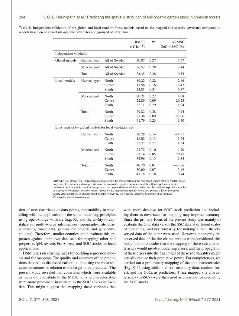
were more decisive for SOC stock prediction and includ-ing them as covariates for mapping may improve accuracy.Since the primary focus of the present study was mainly toevaluate the GoC data versus the SSC data at different scalesof modelling, and not primarily for making a map, the ob-served data of the latter were used. However, since only theobserved data of the site characteristics were considered, thisstudy fails to consider that the mapping of these site charac-teristics would involve modelling errors, and the propagationof these errors into the final maps of these site variables mightactually reduce their predictive power. For completeness, wecarried out a preliminary mapping of the site characteristics(Fig. S11) using additional soil inventory data, random for-est, and the GoCs as predictors. These mapped site charac-teristics (mSSCs) were then used as covariate for predictingthe SOC stocks.



Table 6 presents the error metrics after independent vali-dation for both local and global models, along with the per-centage margin of the RMSE in relation to the models basedon GoCs. First, the local mSSC-based models still recorded alower RMSE compared to global mSSC models. Comparedto the GoC models, the overall positive percentage margin ofthe RMSE for the independent validations indicated that themSSC models recorded the lowest RMSE. However, whenassessing the RMSE margin between the global models ofGoCs and SSCs, negative percentages were mainly recordedfor northern Sweden, independently of the depth. This in-dicated that the mSSC-based global models were less accu-rate at predicting SOC stocks locally in northern Sweden.On the other hand, the mSSC-based local model did presenta better prediction for northern Sweden for the humus layerand mineral SOC stock. The mean SOC predictions basedon the mSSCs showed a stronger increasing gradient fromnorthern to southern Sweden (Fig. S12) compared to thepattern observed with the GoC maps. However, the uncer-tainty distribution was of a similar magnitude (Fig. S12) tothose observed for the maps based on GoCs, probably dueto error propagations, as these covariates were used to makethe site-specific characteristics maps. This suggests that theSSCs should still be supplemented for improvement at thisstage with other covariates different from the GoCs, such asmulti-temporal spectral (e.g. normalized difference vegeta-tion index) data that are able to capture vegetation dynamicin forests. Notwithstanding the possibility of error propaga-tion, the study of which was beyond the scope our focus, thepreceding results tend to confirm the potential of the high-resolution maps of the site characteristics to contribute to theimprovement of SOC stock prediction as compared to usingonly the GoC data. Given that the preliminary mappings ofthe SSCs recorded low kappa (0.17–0.48) values (Fig. S11)at this stage, further improvements are still necessary to im-prove their SOC stock predictive ability and the associatedcoefficient of variations.

5 Conclusion

This study has shown that:

– Local models have a comparative advantage over globalmodels when using either site characteristics alone orthe combination of the latter with a group of covariatesdominated by remotely sensed data.

– Using a group of covariates dominated by remote sens-ing data with a soil inventory data set indicates that suchcovariates have limited predictive ability compared tosite-specific covariates.

– The most important covariates that influence the humuslayer, mineral soil, and total SOC stock were related tothe site-characteristic covariates consisting of the soil

moisture class, vegetation type, soil type, and soil tex-ture.

Code availability. All code has been made available in an R file(.pdf) in the Supplement (Asset S1).

Data availability. The data used in this study are available uponreasonable request to Johan Stendahl ([email protected]). Thehigh-resolution digital elevation models (DEM) should be requestedby contacting the Swedish national mapping agency (Lantmäteriet;https://www.lantmateriet.se, last access: 1 April 2019). The cli-mate data used (MAT and MAP) can be downloaded from World-Clim (https://www.worldclim.org/, Fick and Hijmans, 2017). Thegeochemical and gamma ray data can be obtained from the Ge-ological Survey of Sweden (SGU; https://www.sgu.se, last ac-cess: 25 March 2019). Requests for forest maps should be di-rected to the Swedish Forest Agency (Skogsstyrelsen; https://www.skogsstyrelsen.se, last access: 15 January 2019). The data set re-lated to the historical map series can be freely downloaded from theFigshare repository at https://doi.org/10.17045/sthlmuni.4649854(Auffret et al., 2017b).

Supplement. The supplement related to this article is availableonline at: https://doi.org/10.5194/soil-7-377-2021-supplement.

Author contributions. The conceptualization of the study for thispaper was done by KOLH, with input from JS, ML, and EK. Thedata curation and formal analysis, methodology, and visualizationfor the paper was performed by KOLH, with substantial input fromJS, ML, and EK. KOLH wrote the initial draft, and all authors wereinvolved in the reviewing and editing of the paper.

Competing interests. The authors declare that they have no con-flict of interest.

Disclaimer. Publisher’s note: Copernicus Publications remainsneutral with regard to jurisdictional claims in published maps andinstitutional affiliations.

Acknowledgements. We thank all the reviewers and the editorfor their valuable comments on the paper.

Financial support. This work has been supported by the SwedishResearch Council Formas.

Review statement. This paper was edited by Nicolas P. A. Sabyand reviewed by Madlene Nussbaum and two anonymous referees.


https://www.lantmateriet.se

https://www.worldclim.org/

https://www.sgu.se

https://www.skogsstyrelsen.se

https://www.skogsstyrelsen.se

https://doi.org/10.17045/sthlmuni.4649854

https://doi.org/10.5194/soil-7-377-2021-supplement


References

Andersson, M., Carlsson, M., Ladenberger, A., Morris, G.,Sadeghi, M., and Uhlbäck, J.: Geokemisk Atlas Över Sverige-Geochemical Atlas of Sweden, Sveriges Geologiska Undersökn-ing, Uppsala, Sweden, 2014.

Angelstam, P. and Pettersson, B.: Principles of present Swedish for-est biodiversity management, Ecol. Bull., 46, 191–203, 1997.

Auffret, A. G., Kimberley, A., Plue, J., Skånes, H., Jakobsson, S.,Waldén, E., Wennbom, M., Wood, H., Bullock, J. M., Cousins,S. A., and Gartz, M.: HistMapR: Rapid digitization of his-torical land-use maps in R, Methods Ecol. Evol., 8, 1453–1457, 2017. Auffret, A. G., Kimberley, A., Plue, J., Skånes,H., Jakobsson, S., Waldén, E., Wennbom, M., Wood, H., Bul-lock, J. M., Cousins, S. A. O., Gartz, M., Hooftman, D. A.P., and Tränk, L.: Data from: HistMapR: Rapid digitization ofhistorical land-use maps in R, Stockholm University [data set],https://doi.org/10.17045/sthlmuni.4649854.v2, 2017b.

Beguin, J., Fuglstad, G.-A., Mansuy, N., and Paré, D.: Predictingsoil properties in the Canadian boreal forest with limited data:Comparison of spatial and non-spatial statistical approaches,Geoderma, 306, 195–205, 2017.

Breiman, L.: Random Forests, Mach. Learn., 45, 5–32,https://doi.org/10.1023/A:1010933404324, 2001.

Buchholz, T., Friedland, A. J., Hornig, C. E., Keeton, W. S., Zanchi,G., and Nunery, J.: Mineral soil carbon fluxes in forests and im-plications for carbon balance assessments, GCB Bioenergy, 6,305–311, 2014.

Cao, B., Domke, G. M., Russell, M. B., and Walters, B. F.: Spatialmodeling of litter and soil carbon stocks on forest land in theconterminous United States, Sci. Total Environ., 654, 94–106,2019.

Carreiro, M. M., Sinsabaugh, R. L., Repert, D. A., and Parkhurst,D. F.: Microbial enzyme shifts explain litter decay responses tosimulated nitrogen deposition, Ecology, 81, 2359–2365, 2000.

Ceh, M., Kilibarda, M., Lisec, A., and Bajat, B.: Estimating the per-formance of random forest versus multiple regression for pre-dicting prices of the apartments, SPRS Int. J. Geo-Inf., 7, 168,https://doi.org/10.3390/ijgi7050168, 2018.

Conrad, O., Bechtel, B., Bock, M., Dietrich, H., Fischer, E., Gerlitz,L., Wehberg, J., Wichmann, V., and Böhner, J.: System for Auto-mated Geoscientific Analyses (SAGA) v. 2.1.4, Geosci. ModelDev., 8, 1991–2007, https://doi.org/10.5194/gmd-8-1991-2015,2015.

Dieleman, W. I. J., Venter, M., Ramachandra, A., Krockenberger,A. K., and Bird, M. I.: Soil carbon stocks vary predictably withaltitude in tropical forests: implications for soil carbon storage,Geoderma, 204, 59–67, 2013.

Dowling, T. P., Alexanderson, H., and Möller, P.: The new high-resolution LiDAR digital height model (“Ny Nationell Höjdmod-ell”) and its application to Swedish Quaternary geomorphology,GFF, 135, 145–151, 2013.

Erdi-Krausz, G., Matolin, M., Minty, B., Nicolet, J. P., Reford, W.S., and Schetselaar, E. M.: Guidelines for radioelement mappingusing gamma ray spectrometry data: also as open access e-book,International Atomic Energy Agency (IAEA), Austria, 2003.

Fick, S. E. and Hijmans, R. J.: WorldClim 2: new 1-km spatial reso-lution climate surfaces for global land areas, Int. J. Climatol., 37,

4302–4315, https://doi.org/10.1002/joc.5086, 2017 (data avail-able at: https://www.worldclim.org/, latest access: 20 June 2019).

Forkuor, G., Hounkpatin, O. K. L., Welp, G., and Thiel,M.: High Resolution Mapping of Soil Properties Us-ing Remote Sensing Variables in South-Western BurkinaFaso: A Comparison of Machine Learning and Multi-ple Linear Regression Models, PLoS ONE, 12, e0170478,https://doi.org/10.1371/journal.pone.0170478, 2017.

Framstad, E.: Biodiversity, carbon storage and dynamics of oldnorthern forests, Nordic Council of Ministers, Copenhagen,2013.

Fröberg, M., Tipping, E., Stendahl, J., Clarke, N., and Bryant, C.:Mean residence time of O horizon carbon along a climatic gradi-ent in Scandinavia estimated by 14C measurements of archivedsoils, Biogeochemistry, 104, 227–236, 2011.

Gomes, L. C., Faria, R. M., de Souza, E., Veloso, G. V., Schaefer, C.E. G., and Fernandes Filho, E. I. J. G.: Modelling and mappingsoil organic carbon stocks in Brazil, Geoderma, 340, 337–350,2019.

Grimm, R., Behrens, T., Marker, M., and Elsenbeer, H.: Soil organiccarbon concentrations and stocks on Barro Colorado Island –Digital soil mapping using Random Forests analysis, Geoderma,146, 102–113, https://doi.org/10.1016/j.geoderma.2008.05.008,2008.

Hastie, T., Tibshirani, R. J., and Friedman, J. H.: The elementsof statistical learning: data mining, inference, and prediction,Springer, New York, 2011.

Henderson, B. L., Bui, E. N., Moran, C. J., and Simon, D. A. P.:Australia-wide predictions of soil properties using decision trees,Geoderma, 124, 383–398, 2005.

Hobbie, S. E., Schimel, J. P., Trumbore, S. E., and Randerson, J. R.:Controls over carbon storage and turnover in high-latitude soils,Glob. Change Biol., 6, 196–210, 2000.

Horning, N.: Random Forests: An algorithm for image classificationand generation of continuous fields data sets, in: Proceedings ofthe International Conference on Geoinformatics for Spatial In-frastructure Development in Earth and Allied Sciences, 911, Os-aka, Japan, 2010.

Hounkpatin, O. K., de Hipt, F. O., Bossa, A. Y., Welp, G., andAmelung, W. J. C.: Soil organic carbon stocks and their deter-mining factors in the Dano catchment (Southwest Burkina Faso),Catena, 166, 298–309, 2018.

Hu, Y., Xu, X., Wu, F., Sun, Z., Xia, H., Meng, Q., Huang, W., Zhou,H., Gao, J., and Li, W.: Estimating Forest Stock Volume in HunanProvince, China, by Integrating In Situ Plot Data, Sentinel-2 Im-ages, and Linear and Machine Learning Regression Models, Re-mote Sens., 12, 186, https://doi.org/10.3390/rs12010186, 2020.

Hyvonen, R., Persson, T., Andersson, S., Olsson, B., Agren, G. I.,and Linder, S.: Impact of long-term nitrogen addition on carbonstocks in trees and soils in northern Europe, Biogeochemistry,89, 121–137, https://doi.org/10.1007/s10533-007-9121-3, 2008.

Iwald, J.: Acidification of Swedish forest soils, SLU Service/Repro,Uppsala, 2016.

Jandl, R., Lindner, M., Vesterdal, L., Bauwens, B., Baritz, R., Hage-dorn, F., Johnson, D. W., Minkkinen, K., and Byrne, K. A.: Howstrongly can forest management influence soil carbon sequestra-tion?, Geoderma, 137, 253–268, 2007.

Jenny, H.: Factors of Soil Formation A System of Quantitave Pedol-ogy, Dover Earth Science, 1941.


https://doi.org/10.17045/sthlmuni.4649854.v2

https://doi.org/10.1023/A:1010933404324

https://doi.org/10.3390/ijgi7050168

https://doi.org/10.5194/gmd-8-1991-2015

https://doi.org/10.1002/joc.5086

https://www.worldclim.org/

https://doi.org/10.1371/journal.pone.0170478

https://doi.org/10.1016/j.geoderma.2008.05.008

https://doi.org/10.3390/rs12010186

https://doi.org/10.1007/s10533-007-9121-3


Johansson, B. and Chen, D.: The influence of wind and topographyon precipitation distribution in Sweden: Statistical analysis andmodelling, Int. J. Climatol., 23, 1523–1535, 2003.

Jungqvist, G., Oni, S. K., Teutschbein, C., and Fut-ter, M. N.: Effect of climate change on soil tempera-ture in Swedish boreal forests, PloS one, 9, e93957,https://doi.org/10.1371/journal.pone.0093957, 2014.

Kauppi, P. E., Posch, M., and Pirinen, P.: Large impacts of climaticwarming on growth of boreal forests since 1960, PLoS One, 9,e111340, https://doi.org/10.1371/journal.pone.0111340, 2014.

Kleja, D. B., Svensson, M., Majdi, H., Jansson, P.-E., Langvall, O.,Bergkvist, B., Johansson, M.-B., Weslien, P., Truusb, L., and Lin-droth, A.: Pools and fluxes of carbon in three Norway spruceecosystems along a climatic gradient in Sweden, Biogeochem-istry, 89, 7–25, 2008.

Kuhn, M.: Caret: classification and regression training, Astro-physics Source Code Library, 1, 05003, available at: https://cran.r-project.org/web/packages/caret/index.html (last access:2 July 2021), 2015.

Kuhn, M.: caret: Classification and regression training [Com-puter software manual], available at: https://CRAN.R-project.org/package=caret, last access: 10 April 2019.

Kumar, P., Pandey, P. C., Singh, B. K., Katiyar, S., Mandal, V. P.,Rani, M., Tomar, V., and Patairiya, S.: Estimation of accumu-lated soil organic carbon stock in tropical forest using geospatialstrategy, Egyptian Journal of Remote Sensing and Space Science,19, 109–123, 2016.

Lawrence, I. and Lin, K.: A concordance correlation coefficient toevaluate reproducibility, Biometrics, 45, 255–268, 1989.

Lidberg, W., Nilsson, M., and Ågren, A.: Using machine learning togenerate high-resolution wet area maps for planning forest man-agement: A study in a boreal forest landscape, Ambio, 49, 1–12,2019.

Lützow, M. v., Kögel-Knabner, I., Ekschmitt, K., Matzner, E.,Guggenberger, G., Marschner, B., and Flessa, H.: Stabilizationof organic matter in temperate soils: mechanisms and their rele-vance under different soil conditions – a review, Eur. J. Soil Sci.,57, 426–445, 2006.

Mallik, S., Bhowmik, T., Mishra, U., and Paul, N.: Mapping andprediction of soil organic carbon by an advanced geostatisti-cal technique using remote sensing and terrain data, GeocartoInt., 1–17, https://doi.org/10.1080/10106049.2020.1815864, on-line first, 2020.

Malone, B. P., McBratney, A. B., Minasny, B., and Laslett, G. M.:Mapping continuous depth functions of soil carbon storage andavailable water capacity, Geoderma, 154, 138–152, 2009.

Mansuy, N., Thiffault, E., Paré, D., Bernier, P., Guindon, L., Ville-maire, P., Poirier, V., and Beaudoin, A.: Digital mapping of soilproperties in Canadian managed forests at 250m of resolution us-ing the k-nearest neighbor method, Geoderma, 235, 59–73, 2014.

McBratney, A. B., Santos, M. M., and Minasny, B.: On digital soilmapping, Geoderma, 117, 3–52, 2003.

Meinshausen, N.: Quantile regression forests, J. Mach. Learn. Res.,7, 983–999, 2006.

Millberg, H., Boberg, J., and Stenlid, J.: Changes in fungal commu-nity of Scots pine (Pinus sylvestris) needles along a latitudinalgradient in Sweden, Fungal Ecol., 17, 126–139, 2015.

Minasny, B. and McBratney, A. B.: Digital soil mapping: A briefhistory and some lessons, Geoderma, 264, 301–311, 2016.

Murphy, P. N. C., Ogilvie, J., Castonguay, M., Zhang, C.-f., Meng,F.-R., and Arp, P. A.: Improving forest operations planningthrough high-resolution flow-channel and wet-areas mapping,Forest.Chron., 84, 568–574, 2008.

Nelson, M., Bishop, T., Triantafilis, J., and Odeh, I.: An error budgetfor different sources of error in digital soil mapping, Eur. J. SoilSci., 62, 417–430, 2011.

Nilsson, M., Nordkvist, K., Jonzén, J., Lindgren, N., Axensten, P.,Wallerman, J., Egberth, M., Larsson, S., Nilsson, L., and Eriks-son, J.: A nationwide forest attribute map of Sweden predictedusing airborne laser scanning data and field data from the Na-tional Forest Inventory, Remote Sens. Environ., 194, 447–454,2017.

Nilsson, T. and Lundin, L.: Prediction of bulk density in Swedishforest soils from the organic carbon content and soil depth, Re-ports in Forest Ecology & Forest Soils 91, Swedish University ofAgricultural Sciences, Uppsala, Sweden, 39 pp., 2006.

Ortiz, C. A., Liski, J., Gärdenäs, A. I., Lehtonen, A., Lundblad, M.,Stendahl, J., Ågren, G. I., and Karltun, E. J. E. M.: Soil organiccarbon stock changes in Swedish forest soils – a comparison ofuncertainties and their sources through a national inventory andtwo simulation models, Ecol. Modell., 251, 221–231, 2013.

Ottoy, S., De Vos, B., Sindayihebura, A., Hermy, M., and Van Or-shoven, J.: Assessing soil organic carbon stocks under currentand potential forest cover using digital soil mapping and spatialgeneralisation, Ecol. Indic., 77, 139–150, 2017.

Pan, Y., Birdsey, R. A., Fang, J., Houghton, R., Kauppi, P.E., Kurz, W. A., Phillips, O. L., Shvidenko, A., Lewis,S. L., and Canadell, J. G.: A large and persistent car-bon sink in the world’s forests, Science, 333, 1201609,https://doi.org/10.1126/science.1201609, 2011.

Piikki, K., Wetterlind, J., Söderström, M., and Stenberg, B. J. P.a.: Three-dimensional digital soil mapping of agricultural fieldsby integration of multiple proximal sensor data obtained fromdifferent sensing methods, Precis. Agric., 16, 29–45, 2015.

Piikki, K. and Söderström, M.: Digital soil mapping of arable landin Sweden–Validation of performance at multiple scales, Geo-derma, 352, 342–350, 2019.

Price, D. T., Alfaro, R., Brown, K., Flannigan, M., Fleming, R.,Hogg, E., Girardin, M., Lakusta, T., Johnston, M., and McKen-ney, D.: Anticipating the consequences of climate change forCanada’s boreal forest ecosystems, Environ. Rev., 21, 322–365,2013.

Prietzel, J. and Christophel, D.: Organic carbon stocks in forest soilsof the German Alps, Geoderma, 221, 28–39, 2014.

Schulp, C. J. E., Verburg, P. H., Kuikman, P. J., Nabuurs, G.-J., Olivier, J. G. J., Vries, W., and Veldkamp, T.: Improvingnational-scale carbon stock inventories using knowledge on landuse history, Environ. Manage., 51, 709–723, 2013.

Schulp, E. and Verburg, P. H.: Effect of land use history and sitefactors on spatial variation of soil organic carbon across a phys-iographic region, Agr. Ecosyst. Environ., 133, 86–97, 2009.

SGU: Map generator, available at: http://apps.sgu.se/kartgenerator/maporder_en.html, last access: 25 March 2019.

Sheikh, M. A., Kumar, M., and Bussmann, R. W.: Altitudinal vari-ation in soil organic carbon stock in coniferous subtropical andbroadleaf temperate forests in Garhwal Himalaya, Carbon bal-ance and management, 4, 1–6, 2009.




https://cran.r-project.org/web/packages/caret/index.html

https://cran.r-project.org/web/packages/caret/index.html

https://CRAN.R-project.org/package=caret

https://CRAN.R-project.org/package=caret

https://doi.org/10.1080/10106049.2020.1815864

https://doi.org/10.1126/science.1201609

http://apps.sgu.se/kartgenerator/maporder_en.html

http://apps.sgu.se/kartgenerator/maporder_en.html


Somarathna, P., Malone, B., and Minasny, B.: Mapping soil organiccarbon content over New South Wales, Australia using local re-gression kriging, Geoderma Regional, 7, 38–48, 2016.

Song, X.-D., Wu, H.-Y., Ju, B., Liu, F., Yang, F., Li, D.-C., Zhao, Y.-G., Yang, J.-L., and Zhang, G.-L.: Pe-doclimatic zone-based three-dimensional soil organiccarbon mapping in China, Geoderma, 363, 114145,https://doi.org/10.1016/j.geoderma.2019.114145, 2020.

Stendahl, J., Lundin, L., and Nilsson, T.: The stone and bouldercontent of Swedish forest soils, Catena, 77, 285–291, 2009.

Stendahl, J., Berg, B., and Lindahl, B. D.: Manganese avail-ability is negatively associated with carbon storage in north-ern coniferous forest humus layers, Sci. Rep.-UK, 7, 15487,https://doi.org/10.1038/s41598-017-15801-y, 2017.

Söderström, M. and Eriksson, J.: Gamma-ray spectrometry and ge-ological maps as tools for cadmium risk assessment in arablesoils, Geoderma, 192, 323–334, 2013.

Söderström, M., Sohlenius, G., Rodhe, L., and Piikki, K. J. P. A.:Adaptation of regional digital soil mapping for precision agricul-ture, Precision Agriculture, 17, 588–607, 2016.

Tang, X., Xia, M., Pérez-Cruzado, C., Guan, F., and Fan, S.J. S. R.: Spatial distribution of soil organic carbon stockin Moso bamboo forests in subtropical China, 7, 42640,https://doi.org/10.1038/srep42640, 2017.

Tranter, G., Jarvis, N., Moeys, J., and Söderström, M.: Broad-scaledigital soil mapping with geographically disparate geophysicaldata: A Swedish example, Geophys. Res. Abstr., EGU2011-7538, EGU General Assembly 2011, Vienna, Austria, 2011.

Wang, B., Waters, C., Orgill, S., Cowie, A., Clark, A., Li Liu, D.,Simpson, M., McGowen, I., and Sides, T.: Estimating soil or-ganic carbon stocks using different modelling techniques in thesemi-arid rangelands of eastern Australia, Ecol. Indic., 88, 425–438, 2018.

Vasques, G. M., Coelho, M. R., Dart, R. O., Oliveira, R. P., andTeixeira, W. G.: Mapping soil carbon, particle-size fractions, andwater retention in tropical dry forest in Brazil, Pesqui. Agropecu.Bras., 51, 1371–1385, 2016.

Vaysse, K. and Lagacherie, P. J. G.: Using quantile regression for-est to estimate uncertainty of digital soil mapping products, Geo-derma, 291, 55–64, 2017.

Wiesmeier, M., Barthold, F., Blank, B., and Kögel-Knabner, I.: Dig-ital mapping of soil organic matter stocks using Random Forestmodeling in a semi-arid steppe ecosystem, Plant Soil, 340, 7–24,https://doi.org/10.1007/s11104-010-0425-z, 2011.

Wiesmeier, M., Urbanski, L., Hobley, E., Lang, B., von Lützow, M.,Marin-Spiotta, E., van Wesemael, B., Rabot, E., Ließ, M., andGarcia-Franco, N.: Soil organic carbon storage as a key functionof soils-A review of drivers and indicators at various scales, Geo-derma, 333, 149–162, 2019.

Yam, G., Tripathi, O. P., and Das, D. N.: Modelling of total soil car-bon using readily available soil variables in temperate forest ofEastern Himalaya, Northeast India, Geology Ecology and Land-scapes, https://doi.org/10.1080/24749508.2019.1706295, onlinefirst, 2019.

Zak, D. R.: Molecular and Microbial Mechanisms Increasing SoilC Storage Under Future Rates of Anthropogenic N Deposition,Univ. of Michigan, Ann Arbor, MI, USA, 2017.

Zhang, H., Goll, D. S., Wang, Y. P., Ciais, P., Wieder, W. R.,Abramoff, R., Huang, Y., Guenet, B., Prescher, A. K., and Vis-carra Rossel, R. A.: Microbial dynamics and soil physicochem-ical properties explain large-scale variations in soil organic car-bon, Glob. Change Biol., 26, 2668–2685, 2020.


https://doi.org/10.1016/j.geoderma.2019.114145

https://doi.org/10.1038/s41598-017-15801-y

https://doi.org/10.1038/srep42640

https://doi.org/10.1007/s11104-010-0425-z

https://doi.org/10.1080/24749508.2019.1706295

Documents

Predicting the spatial distribution of soil organic carbon