Embed Size (px)
Citation preview

ORE Open Research Exeter
TITLE
Predicting thermal response of bridges using regression models derived from measurementhistories
AUTHORS
Kromanis, Rolands; Kripakaran, Prakash
JOURNAL
Computers and Structures
DEPOSITED IN ORE
01 April 2015
This version available at
http://hdl.handle.net/10871/16644
COPYRIGHT AND REUSE
Open Research Exeter makes this work available in accordance with publisher policies.
A NOTE ON VERSIONS
The version presented here may differ from the published version. If citing, you are advised to consult the published version for pagination, volume/issue and date ofpublication

Predicting Thermal Response of Bridges Using Regression Models Derived
from Measurement Histories
Rolands Kromanis*, Prakash Kripakaran
College of Engineering, Mathematics and Physical Sciences, University of Exeter, Exeter, UK
E-mail: [email protected]
Abstract: This study investigates the application of novel computational techniques for structural
performance monitoring of bridges that enable quantification of temperature-induced response
during the measurement interpretation process. The goal is to support evaluation of bridge
response to diurnal and seasonal changes in environmental conditions, which have widely been
cited to produce significantly large deformations that exceed even the effects of live loads and
damage. This paper proposes a regression-based methodology to generate numerical models,
which capture the relationships between temperature distributions and structural response, from
distributed measurements collected during a reference period. It compares the performance of
various regression algorithms such as multiple linear regression (MLR), robust regression (RR)
and support vector regression (SVR) for application within the proposed methodology. The
methodology is successfully validated on measurements collected from two structures – a
laboratory truss and a concrete footbridge. Results show that the methodology is capable of
accurately predicting thermal response and can therefore help with interpreting measurements
from continuous bridge monitoring.
1. Introduction
Rising expenditure on bridge maintenance has led to significant interest in sensing technology
and in its potential to lower lifecycle costs of bridge management. Current bridge monitoring
systems greatly simplify the collection, storage and transmission of measurements, and such
systems are increasingly installed on bridges around the world. Notable examples are the
Stonecutters bridge in Hong Kong [1] that is continuously monitored using over 1200 sensors
and the St. Anthony Falls bridge in Minnesota, USA [2] that has over three hundred sensors.
Monitoring systems on these structures continuously measure a number of bridge parameters
related to the structures’ response and its environment. The management and interpretation of
the collected data, however, poses a great challenge to bridge engineers.
Data interpretation techniques currently employed in practice are often simplistic and tend to
be unreliable. For example, the approach typically adopted to analyze measurements from
bridge monitoring is to check whether collected measurements exceed pre-defined threshold
values and to send email or text notifications to bridge engineers when such situations occur.
However, specifying threshold values such that a monitoring system is sensitive to damage
while not producing excessive false alarms is seldom possible. The development of robust and
reliable strategies for measurement interpretation is therefore increasingly accepted as central
to the practical uptake of structural health monitoring (SHM) [3, 4]. Such strategies are also
envisioned to be a fundamental element of the future “smart” infrastructures [3, 5, 6] that are
expected to take advantage of recent advances in wireless sensing [7] and energy harvesting
technologies [8].
Response measurements (e.g., strains) taken from bridges comprise the effects of several
types of loads including vehicular traffic and ambient conditions. Hence an important step in
measurement interpretation is characterizing the influences of the individual load components
on collected measurements. This research addresses the challenge of accounting for the
thermal response in measurements collected during quasi-static monitoring of bridges.
Previous long-term monitoring studies have illustrated that daily and seasonal temperature

variations have a great influence on the structural response of bridges [1, 9], and that this
influence may even exceed the response to vehicular traffic. Catbas et al. [10] monitored a
long-span truss bridge in the USA and observed that the annual peak-to-peak strain
differentials for the bridge were ten times higher than the maximum traffic-induced strains.
Measurements from long-term monitoring of the Tamar Bridge in the UK showed that
thermal variations caused the majority of the observed deformations in the structure (Koo et
al., 2012). While this paper is concerned mainly with quasi-static measurements, temperature
variations are also known to have noticeable effects on the vibration characteristics of bridges.
Cross et al. [11] investigated temperature effects on the dynamic response of Tamar bridge
and showed that ambient temperature significantly influences seasonal alterations in the
structure’s fundamental frequency. Ni et al. [12] and Hua et al. [9] showed that the modal
properties such as frequencies are highly correlated with ambient temperatures for the Ting
Kau bridge. These studies highlight the importance of temperature effects on long-term
structural behaviour. In the context of monitoring, they also emphasize the need for
systematic ways of accounting for temperature effects in the measurement interpretation
process.
Existing measurement interpretation techniques can be broadly classified into two categories
[4] – (1) Model-based (physics-based) methods and (2) Data-driven (non physics-based)
methods. Model-based methods rely on behavioural models (e.g., finite element (FE) models)
that are derived from the fundamental physics of the structure. Their application to
interpreting measurements from continuous structural health monitoring is limited due to their
larger computational requirements and the difficulty in generating reliable behaviour models
that are representative of the structure [10, 13]. In contrast to model-based methods, data-
driven methods operate directly on measurements and require minimal structural information.
They especially show promise for anomaly detection due to their capability for recognizing
and tracking patterns in measurement time-series. Data-driven methods use available
measurements to first establish baseline criteria for structural behaviour, i.e., to define
conditions that identify with normal structural behaviour. For example, measurements
collected shortly after a bridge is built or refurbished could help determine baseline
conditions. Subsequent measurements are assessed in real-time to detect deviations from these
conditions. This research aims to develop computational approaches for evaluating the
thermal response of bridges that are suitable for subsequent embedment within data-driven
methods for measurement interpretation.
Data-driven methods are typically based on statistical or signal processing techniques such as
moving principal component analysis [14] and wavelet transforms [15]. Existing data-driven
approaches focus on the analysis of response measurements and ignore distributed
temperature measurements. Omenzetter and Brownjohn [16] applied autoregressive integrated
moving average models (ARIMA) to analyze strain histories from a full-scale bridge and
noted that performance of the models could potentially be improved by including temperature
measurements. More recently, Posenato et al. [14] exploited the correlations between
response measurements due to seasonal temperature variations for anomaly detection.
However, their approach was shown to be sensitive for only high levels of damage. Studies
have also treated the effects of temperature variations on structural behaviour as noise
superimposed on the traffic-induced response. Laory et al. [17]showed that filtering the
effects of diurnal and seasonal temperature changes from response measurements may lead to
information loss and hence minimize the chances of detecting anomalies. These results
support the development of anomaly detection techniques that explicitly model the
relationships between thermal response and distributed temperature measurements. To
develop such techniques, systematic approaches for building numerical models that are

capable of predicting thermal response from distributed temperature measurements are
required. This research is a step in that direction.
This paper presents a generic computational approach to evaluate the thermal response of
bridges from distributed temperature measurements. The premise of the approach is that a
reference set of temperature and response measurements could help train regression-based
models for thermal response prediction. This study compares a number of algorithms for
model generation including multiple linear regression, support vector regression and artificial
neural networks. The goal is to arrive at an approach that leads to robust models that are
capable of providing accurate response predictions even when there are noise and outliers in
the measurements.
The rest of the paper is organized as follows. The envisioned framework for incorporating
thermal effects in the measurement interpretation process is first presented. The proposed
approach and the various algorithms that are evaluated for model generation within the
approach are then outlined. The two structures – (i) a laboratory truss and (ii) a footbridge at
the National Physical Laboratory (NPL), which form the case studies in this research, are
described. The performance of the developed approach is studied on measurements from these
two structures. Lastly, results are summarized with important conclusions.
2. Temperature effects in bridges
Most materials expand or contract under changes in temperature. Therefore bridges and other
civil structures continuously deform under temperature distributions that are introduced in
them by ambient weather conditions. Temperature distributions across full-scale structures
could be very complex depending upon various factors such as their geographic location, their
shape and orientation, and the surrounding environment. Temperature gradients in bridges are
often non-linear [18] such that they introduce thermal stresses even in bridge girders with
simple supports. Potgieter and Gamble [18] showed using measurements from an existing box
girder bridge that stresses and forces due to nonlinear temperature distributions are often of
magnitudes comparable to those due to live loads. Bridge engineers therefore give significant
importance to thermal effects and consequently, bridge designs either incorporate ways of
accommodating thermal movements (e.g. expansion joints) or take into account the stresses
that could be created by obstruction to thermal movements (e.g. integral bridges). Due to the
difficulty in predicting the temperature distributions that could be experienced by as-built
structures at the design stage, engineers typically assume linear temperature gradients as
indicated by current design codes to evaluate their thermal response. The same approach is,
however, not appropriate for interpreting measurements from long-term monitoring since a
significant component of response measurements will be due to temperature variations. For
example, consider the plot in Figure 1 showing daily variations in bearing displacements for
the Cleddau Bridge in Wales. The figure clearly shows that the displacement increases during
the day as the temperature rises with dawn and then decreases later in the day with sunset.
Moreover, measurements collected over a year (not shown in figure) reveal that the
displacements closely follow the seasonal variations in temperatures.

Figure 1: The Cleddau Bridge (top), time series of displacement measurements collected at a bearing
over 1 day (bottom left) and a closer look at the measurements taken over 2 hours (bottom right).
(Courtesy: Bill Harvey Associates and Pembrokeshire County Council).
The premise of this study is that temperature effects have to be factored into the measurement
interpretation process for the early and reliable detection of abnormal changes in bridge
behaviour. This study therefore proposes strategies for predicting and accounting for the
thermal response during the measurement interpretation process. The developed strategies
will support a bridge management paradigm that is schematically illustrated in Figure 2. A
bridge like any structural system exhibits responses that vary according to the applied loads.
Loads could be of several types such as vehicular traffic, snow, wind and temperature. A
continuous monitoring system measures the integrated structural response (e.g. strains,
displacements) of the system to all applied static and dynamic loads. The collected
measurements may undergo a preliminary analysis depending on the computing power
available on-site and then transmitted to remote servers via the internet or other
communication modes. These measurements may be transformed and analyzed through a
number of stages of measurement interpretation ranging from initial pre-processing to
complex data fusion in order to infer structural performance. This research deals with the
development of measurement interpretation strategies to support this part of the bridge
management cycle. Results from measurement interpretation may then be presented via
suitable interfaces so that engineers are able to plan and prioritize interventions to ensure
optimal structural performance.
00:00 06:00 12:00 18:00 00:000
5
10
15
20
25
30
35
Beari
ng
dis
pla
cem
en
t (m
m)
Time (HH:MM)06:00 07:00 08:00
5.5
6
6.5
7B
eari
ng
dis
pla
cem
en
t (m
m)
Time (HH:MM)
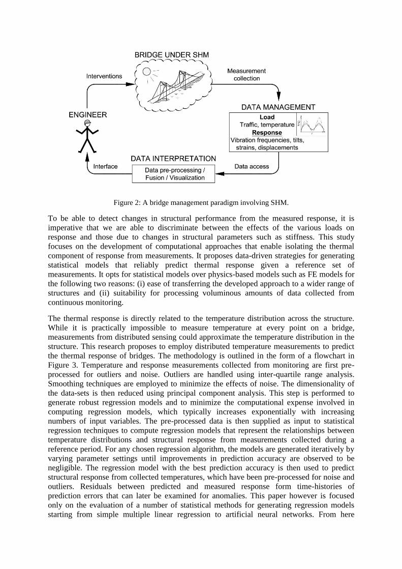
Figure 2: A bridge management paradigm involving SHM.
To be able to detect changes in structural performance from the measured response, it is
imperative that we are able to discriminate between the effects of the various loads on
response and those due to changes in structural parameters such as stiffness. This study
focuses on the development of computational approaches that enable isolating the thermal
component of response from measurements. It proposes data-driven strategies for generating
statistical models that reliably predict thermal response given a reference set of
measurements. It opts for statistical models over physics-based models such as FE models for
the following two reasons: (i) ease of transferring the developed approach to a wider range of
structures and (ii) suitability for processing voluminous amounts of data collected from
continuous monitoring.
The thermal response is directly related to the temperature distribution across the structure.
While it is practically impossible to measure temperature at every point on a bridge,
measurements from distributed sensing could approximate the temperature distribution in the
structure. This research proposes to employ distributed temperature measurements to predict
the thermal response of bridges. The methodology is outlined in the form of a flowchart in
Figure 3. Temperature and response measurements collected from monitoring are first pre-
processed for outliers and noise. Outliers are handled using inter-quartile range analysis.
Smoothing techniques are employed to minimize the effects of noise. The dimensionality of
the data-sets is then reduced using principal component analysis. This step is performed to
generate robust regression models and to minimize the computational expense involved in
computing regression models, which typically increases exponentially with increasing
numbers of input variables. The pre-processed data is then supplied as input to statistical
regression techniques to compute regression models that represent the relationships between
temperature distributions and structural response from measurements collected during a
reference period. For any chosen regression algorithm, the models are generated iteratively by
varying parameter settings until improvements in prediction accuracy are observed to be
negligible. The regression model with the best prediction accuracy is then used to predict
structural response from collected temperatures, which have been pre-processed for noise and
outliers. Residuals between predicted and measured response form time-histories of
prediction errors that can later be examined for anomalies. This paper however is focused
only on the evaluation of a number of statistical methods for generating regression models
starting from simple multiple linear regression to artificial neural networks. From here
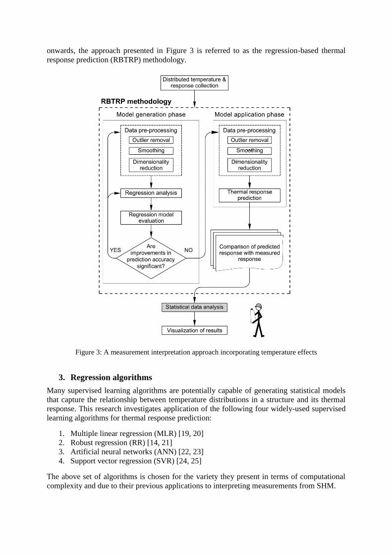
onwards, the approach presented in Figure 3 is referred to as the regression-based thermal
response prediction (RBTRP) methodology.
Figure 3: A measurement interpretation approach incorporating temperature effects
3. Regression algorithms
Many supervised learning algorithms are potentially capable of generating statistical models
that capture the relationship between temperature distributions in a structure and its thermal
response. This research investigates application of the following four widely-used supervised
learning algorithms for thermal response prediction:
1. Multiple linear regression (MLR) [19, 20]
2. Robust regression (RR) [14, 21]
3. Artificial neural networks (ANN) [22, 23]
4. Support vector regression (SVR) [24, 25]
The above set of algorithms is chosen for the variety they present in terms of computational
complexity and due to their previous applications to interpreting measurements from SHM.

3.1. Multiple linear regression (MLR)
MLR is fundamentally an extension of the concept of simple linear regression. In simple
regression, available measurements of a dependent variable (y) and an explanatory variable
(x) are used to generate a function that can later be used to forecast values for the dependent
variable given values for the explanatory variable. However, in many engineering scenarios,
multiple explanatory variables may have to be taken together to accurately predict values for a
dependent variable [26] and this is accommodated by MLR. The general form of the MLR
model (i.e., equation relating the dependent and the explanatory variables) can be expressed
as follows:
(1)
yi is the predicted value of the dependent variable y for the ith
time step; n is the number of
explanatory variables; are the values for the explanatory variables (x1, x2, ... xn)
at the ith
time step; is the intercept and are regression weights. The values for
are computed to minimize an error function based on least-squares estimates. In this study,
y represents a thermal response parameter such as displacement or strain at a specific location.
(x1, x2, ... xn) represent parameters derived from the temperature measurements recorded by
available sensors.
3.2. Robust regression (RR)
Regression techniques typically use a least-squares fitting criterion to identify values for the
parameters in the regression model. However, this criterion is known to be sensitive to the
presence of outliers in the datasets and may therefore lead to unreliable models [27]. RR
mitigates this problem by employing a fitting criterion that eliminates outlier-induced bias in
the regression model. This criterion is often implemented as a weighted least-squares function
where weights are assigned to individual data-sets. The values for the weights are determined
in an iterative manner. Initially identical values are assigned to all of them. In subsequent
iterations, new values are chosen for the weights based on the errors in model predictions
such that higher values are given to data-sets that produce more accurate predictions. This
process is terminated when there are minimal changes to the values of the weights between
iterations.
3.3. Artificial neural networks (ANN)
ANNs [28], which are inspired by biological neural systems, are a powerful way of producing
nonlinear regression models between a number of input and output parameters using large
numbers of training sets. A neural network consists of neurons that are inter-connected in
various layers. The connections between the neurons have weights associated with them and
these are calibrated during training to capture the actual relationship between the input and
output parameters. In this research, ANNs are simulated using MATLAB’s [29] neural
network toolbox. A key step is the selection of an appropriate architecture of the network that
maximizes its efficiency, i.e., use low computational resources while achieving high
prediction accuracy [30]. Similar research in SHM on the application of ANNs for data
interpretation recommend using a hidden layer composed of between 3 and 30 neurons [31,
32]. The number of neurons for the hidden layer can also be defined from a general rule-of-
thumb N1/3
, where N is the number of input points [33]. This study uses a multi-layer feed-
forward neural network that implements the back-propagation rule. It has one hidden layer
and one output layer of a linear neuron. The optimal number of neurons for the hidden layer is
found through a trial and error approach that gradually increases the number of neurons while

evaluating the performance of the ANN on both training and test sets. A hidden layer of 10
neurons is observed to produce consistently good results. The input parameters to the ANN
are derived from distributed temperature measurements. The output parameters are response
values (e.g. strains, tilts) at specific locations on the structure.
3.4. Support vector regression (SVR)
Support vector machines (SVM) are a class of powerful supervised learning algorithms that
are widely used for statistical learning and pattern recognition. The origins of statistical
learning theory including the basic principles of SVM can be tracked to the 1960s when it was
first introduced by Vladimir Vapnik [34]. These concepts have since been further developed
and successfully applied to a range of subject domains such as finance, computer networks
and fault detection [34, 35]. This research employs SVM in its regression mode, which is
often referred to as support vector regression (SVR). In brief, the main steps in SVR are (i)
generation of a vector mapping from the input space to a feature space using kernels, (ii)
construction of a separating hyperplane in the feature space and (iii) introduction and
modification of a loss function. Further details on the SVM approach are provided in
Kromanis and Kripakaran [25].
4. Case studies
This research investigates the application of RBTRP methodology on measurements collected
from two structures: a laboratory truss and the National Physical Laboratory (NPL)
footbridge. The former is used to develop and validate the proposed ideas. The latter is used
primarily to highlight the scalability of the developed methodology.
4.1. Laboratory truss
An aluminium truss (Figure 4) that is representative of trusses commonly used in short span
railway bridges has been fabricated at Exeter as a laboratory-scale structure for this research.
The truss is composed of aluminium elements inter-connected with six high strength steel
bolts at the joints. Two channel sections, each of size , arranged in
the shape of an “I”, form the top and bottom chords as well as the two end–diagonal elements
that connect the top and bottom chords. The other elements are made up of flat bars of size
. The truss is connected to concrete blocks which are fully fixed to the steel
floor, thus, preventing both ends of the truss from any horizontal translation.
Figure 4: Photograph showing the truss and the infra-red heater

An infrared heater, with a maximum output of 2kW, is installed close to the truss. The vertical
and horizontal distances between the heater and the middle of the top-chord of the truss are
0.5m and 0.15m respectively (see Figure 5). The heater is connected to a timer that switches it
on automatically for a period of one hour every three hours to approximately emulate diurnal
temperature variations; in this experiment, one simulated day lasts 3 hours. As shown in
Figure 5, strain and temperature sensors are installed at a number of locations on the truss.
Strain sensors are simple resistance-based strain gauges. Material temperature is monitored
using K-type thermocouples and thermistors; both provide precise temperature measurements.
These sensors are connected to a data-logger unit that is programmed to record measurements
every 5 minutes.
Figure 5: A sketch of the laboratory structure showing its dimensions and the locations of installed
thermocouples (TEMP-i ) and strain gauges (S-i ).
This paper employs measurements collected over a period of 16 days. In total, 4590
measurements have been taken with each of the 15 sensors. Changes in the material
temperature and strains are influenced by variations in the ambient temperature in the
laboratory and by the radiation from the heater (see Figure 5). The range of temperature and
strain values recorded during the monitoring period is provided in Tables 1 and 2. As would
be expected, the ranges of temperature and strain measurements are largest at the sensors
closer to the heater (Tables 1 and 2 – shaded columns). Data in Tables 1 and 2 confirm that
the experiments produce temperature gradients in the truss and therefore result in thermal
deformations. Strains measured at sensor S-4 and ambient temperature are plotted in Figure 6.
The short, cyclic variations of the strains in the figure are due to the operation of the infra-red
heat lamps. The variations in the moving average of the strain time-series are induced by the
daily variations in ambient temperature.
Table 1: Maximum and minimum temperatures from the laboratory truss
Temperature sensor (TEMP-i)
i 1 2 3 4 5 6 7 8 9 10 11
Max (°C) 20.7 21.8 24.5 21.3 21.0 21.0 22.0 30.3 28.1 20.9 21.7
Min (°C) 14.9 15.2 15.2 15.2 16.0 15.6 15.9 16.1 16.1 16.0 16.2
Range (°C) 5.8 6.5 9.3 6.1 5.0 5.4 6.2 14.2 12.0 4.8 5.5
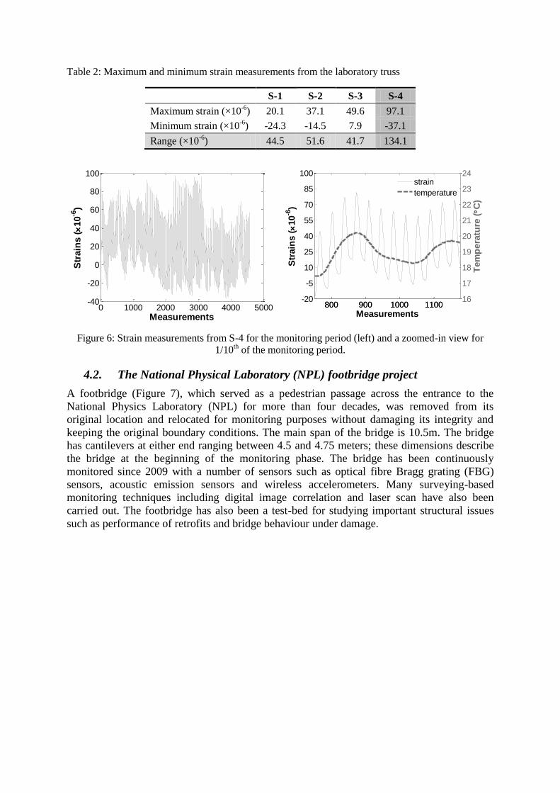
Table 2: Maximum and minimum strain measurements from the laboratory truss
S-1 S-2 S-3 S-4
Maximum strain (×10-6
) 20.1 37.1 49.6 97.1
Minimum strain (×10-6
) -24.3 -14.5 7.9 -37.1
Range (×10-6
) 44.5 51.6 41.7 134.1
Figure 6: Strain measurements from S-4 for the monitoring period (left) and a zoomed-in view for
1/10th of the monitoring period.
4.2. The National Physical Laboratory (NPL) footbridge project
A footbridge (Figure 7), which served as a pedestrian passage across the entrance to the
National Physics Laboratory (NPL) for more than four decades, was removed from its
original location and relocated for monitoring purposes without damaging its integrity and
keeping the original boundary conditions. The main span of the bridge is 10.5m. The bridge
has cantilevers at either end ranging between 4.5 and 4.75 meters; these dimensions describe
the bridge at the beginning of the monitoring phase. The bridge has been continuously
monitored since 2009 with a number of sensors such as optical fibre Bragg grating (FBG)
sensors, acoustic emission sensors and wireless accelerometers. Many surveying-based
monitoring techniques including digital image correlation and laser scan have also been
carried out. The footbridge has also been a test-bed for studying important structural issues
such as performance of retrofits and bridge behaviour under damage.
0 1000 2000 3000 4000 5000-40
-20
0
20
40
60
80
100
Str
ain
s (10
-6)
Measurements
800 900 1000 1100-20
-5
10
25
40
55
70
85
100
Str
ain
s (10
-6)
Measurements
800 900 1000 110016
17
18
19
20
21
22
23
24
Tem
pera
ture
(C
)
strain
temperature

Figure 7: Front view of the NPL footbridge (left) and back view of mid-section of the footbridge
(right) and a tilt-meter (circled).
This study draws upon tilt and temperature measurements from 4 tilt sensors and 10 vibrating
wire strain gauges with temperature sensors. Since this paper uses only the temperature
measurements from the vibrating wire strain gauges, we here onwards refer to these sensors
as temperature sensors. Technical details of the sensors are provided in Table 3 and their
locations are illustrated in Figure 8.
Table 3: Technical specifications of the tilt and temperature sensors employed in the monitoring of the
NPL footbridge
Sensor Specifications
Electrolevel surface mount
tilt meter
Range: ±45 Arc Minutes (±13mm/m)
Resolution: 5.2×10⁻³
mm/m
Vibrating wire arc-
weldable strain gauge*
with temperature sensor
Temperature range: -20 to 80°C
Thermistor resolution: ±0.01°C
*Strain measurements are not considered in this study.

Figure 8: Location of sensors and principal dimensions of the NPL footbridge. TEMP – temperature
sensor; TL – tilt sensors. TL-2 and TL-3 are shown in Figure 7 (right (circled)).
The frequency of measurement collection has varied between 1 and 60 measurements per
hour over the six months of monitoring due to various circumstances related to the work
carried out on the structure. Monitoring was also briefly suspended for a few days. However,
for ease of data management, this study considers only the measurements taken at 5-minute
intervals and ignores the rest. This results in 30,448 measurements for each sensor.
In contrast to the laboratory structure, the NPL footbridge is exposed to naturally varying
environmental conditions and monitored for a longer period. Hence measurements reflect the
effects of diurnal and seasonal variations in temperatures. Capturing the full range of tilt and
temperature variations requires measurements taken over a six-month period, i.e., from peak
winter to peak summer. However, only measurements taken during the first 6 months are
useful to validate the proposed methodology since damage and other experimental work
affecting the behaviour of the structure is known to be undertaken after this initial period. We
overcome this issue by extrapolating the data-set originally collected over duration of six
months to two years. This is done by taking advantage of the high frequency of measurement
collection as follows. Two data sets (D1 and D2) of equal size are first generated from the
original dataset (D). Odd-numbered items in the original time-series D of measurements form
D1. The even-numbered items are mirrored about the 6-month timeline and this forms D2. D2
is appended to D1 hence creating a new data-set E, which emulates approximately one full
season, i.e., 1 year. The process is repeated for E by mirroring half its data-set about the 1-
year timeline and, as a result, a data-set having duration of two years is created. In this
manner, temperature and tilt measurements collected from all the sensors over 6 months are
extrapolated to two years. These data-sets are used to validate the RBTRP methodology.
Measurements from the tilt meters TL-1, TL-2, TL-3 and TL-4 are plotted in Figures 9 and 10
and the maximal and minimal tilt values that they recorded are listed in Table 4. TL-1 and
TL-4 are located on the two cantilevered ends of the footbridge; thus, the tilt measurements
from the two sensors have similar magnitudes but in opposite directions (see Figure 9). In
contrast, measurements from TL-2 and TL-3, which are located just to the right of mid-span
of the footbridge, have similar patterns (see Figure 10).

Figure 9: Tilt measurements from sensors TL-1 (left) and TL-4 (right) on the NPL footbridge
Figure 10: Tilt measurements from sensors TL-2 (left) and TL-3 (right) on the NPL footbridge
Table 4: Maximum and minimum tilt measurements from the NPL footbridge
TL-1 TL-2 TL-3 TL-4
Minimum tilt (mm/m) 0.76 0.70 0.80 1.94
Maximum tilt (mm/m) -1.81 -0.12 -0.15 -1.81
Range (mm/m) 2.57 0.82 0.95 3.75
Seasonal variations in ambient temperatures are discernible in Figure 11 where the time-series
of temperatures collected by sensor TEMP-6 are plotted. The temperature distribution across
a structure is also dependent on the local environmental conditions. One side of the footbridge
is closer to nearby trees (see Figure 7) and is hence relatively less exposed to the sun. This
aspect results in one side of the bridge experiencing much higher temperatures than the other.
This is evident from Table 5, which lists the maximum and minimum temperatures measured
by the various sensors over the considered monitoring period. Sensors TEMP1, TEMP-3 and
TEMP-5, which are in the shade, measure significantly lower maximum temperatures than the
others.
0 0.5 1 1.5 2 2.5 3
x 104
-1.5
-1
-0.5
0
0.5
Measurements
Tilt
(m
m/m
)
0 0.5 1 1.5 2 2.5 3
x 104
-1.5
-1
-0.5
0
0.5
1
1.5
2
Measurements
Tilt
(m
m/m
)
0 0.5 1 1.5 2 2.5 3
x 104
-0.1
0
0.1
0.2
0.3
0.4
0.5
0.6
0.7
Measurements
Tilt
(m
m/m
)
0 0.5 1 1.5 2 2.5 3
x 104
-0.2
0
0.2
0.4
0.6
0.8
Measurements
Tilt
(m
m/m
)

Figure 11: Temperature measurements from sensor TEMP-6 on the NPL footbridge
Table 5: Maximum and minimum temperatures measured by sensors TEMP-1 to TEMP-10 on the
NPL footbridge
Temperature sensor (TEMP-i)
i 1 2 3 4 5 6 7 8 9 10
Max (°C) 26.8 31.2 27.7 31.7 26.3 33.6 33.4 35.0 34.5 35.4
Min (°C) -6.3 -6.6 -6.5 -6.4 -6.3 -6.4 -6.2 -6.5 -6.5 -6.4
Range (°C) 33.1 37.8 34.2 38.1 32.6 40.0 39.6 41.4 41.0 41.8
5. Data pre-processing
5.1. Outliers and noise
Data pre-processing is an essential first step in the measurement interpretation process. In this
study, raw data sets are pre-processed to handle outliers and noise [36]. The resulting data is
subsequently used to generate regression models. The pre-processing step is essential to
generate regression models with high prediction accuracy. The data pre-processing phase is
illustrated in Figure 3. In the first stage of this phase, outliers are identified and replaced with
appropriate values. This research employs moving windows of specified sizes to determine
outliers. Inter-quartile range (IQR) analysis is used to classify if the value at the centre of a
moving window is an outlier by comparing it to other values within that window. If the value
is classified as an outlier, it is replaced by the median value of the moving window [14, 25].
Noise in measurements is then reduced by smoothing the data using moving averages [37].
Measurements of both the laboratory truss and the NPL footbridge are pre-processed using
IQR analysis and smoothing with moving windows of 12 measurements. This has been found
to replace potential outliers and average noisy data more efficiently than smaller or larger
sized windows. Examples of raw and pre-processed strain and temperature measurements
from the laboratory truss are given in Figure 12. Strain recordings are often significantly
noisier than temperatures and hence smoothing strain measurements is particularly important
for generating accurate regression models.
0 0.5 1 1.5 2 2.5 3
x 104
0
10
20
30
40
Measurements
Tem
pera
ture
(C)

Figure 12: Strain and temperature measurements from sensors S-2 (left) and TEMP-3 (right) on the
laboratory truss before and after outlier pre-processing.
5.2. Training and test sets
The testing and training sets are generated differently for the two structures due to the
difference in the quality and quantity of measurements collected from them. The size of the
data set from the laboratory structure is considerably smaller than the one from the NPL
footbridge. The truss is kept indoors and therefore not exposed to ambient effects such as
sunlight, rain and wind. The seasonal temperature effects are also minimal since
measurements from only a 16-day period are used in this study. For this structure,
measurements are equally divided into testing and training sets. Measurements taken over the
first 7 days, which make up a total of 2000 data-points, constitute the training set. The
remaining 2590 measurements are used to evaluate the performance of the proposed
algorithms.
The measurement histories from the NPL footbridge show strong seasonal trends since the
structure is monitored for a longer period and is also exposed to the outside environment. One
year of measurements is required to train adequate regression models. This data-set is hence
split into two equal halves: the first half, which is composed of 15,244 time-points and
corresponds to duration of almost one year, forms the training set and the second half is used
to validate the proposed methodology.
5.3. Dimensionality reduction
Reducing the dimensionality of data-sets can help speed up the model generation process and
also lead to robust regression models. Principal component analysis (PCA) [38] is a widely-
employed statistical technique that takes advantage of inherent correlations between variables
in the data-set for dimensionality reduction. It first involves finding a set of principal
component (PC) vectors that define an orthogonal transformation from the original set of
linearly-correlated variables to a new set of uncorrelated variables. Then, a small number of
PC vectors, which is known to sufficiently capture the variance in the original data, is chosen
to transform the raw data to a low-dimensional PC space.
In this research, PC vectors are first estimated from measurements taken from all temperature
sensors over the training period and then used to transform newly collected temperatures to
PC space. The transformed data is then given as input to the regression models for thermal
response prediction. Dimensionality reduction can, however, negatively impact the accuracy
550 600 650 700 750 800 850
0
10
20
30
40
Measurements
Str
ain
s (10
-6)
before pre-processing
after pre-processing
550 600 650 700 750 800 850
18
20
22
24
Measurements
Tem
pera
ture
(C
)
before pre-processing
after pre-processing

of the regression models. Therefore, this research investigates the relationship between the
number of chosen PC vectors and the performance of the generated regression models.
The general equation describing PCA is as follows:
(2)
D, X, P and M are matrices where D stands for the original set of data-points, X for the scores,
i.e., the equivalent values in PC space, P for the set of principal components and M for the
mean values of the variables. As applied to this work, D of size m×n represents the time-
series of temperature measurements with m and n denoting the number of temperature sensors
and measurements respectively in a moving window; X of size n×c denotes the matrix of
scores with c indicating the number of PCs chosen. After computing the PC vectors from the
training set, subsequent measurements of real-time temperatures collected at any time-step i
are transformed to PC space using the following equation:
(3)
6. Results
6.1. Predicted response
The various algorithms for generating regression models such as MLR, RR, ANN and SVR
are compared in terms of the average prediction error (ey), which is derived from the predicted
( ) and measured ( ) response using the following equation:
(4)
n is the number of measurements in the test set and i is the measurement time-step.
6.1.1. Laboratory structure
The RBTRP methodology is first evaluated on measurement sets from the laboratory
structure. Dimensionality reduction is performed on both raw data-sets and data-sets that have
been pre-processed for outliers and noise. Models for thermal response prediction are
generated using all discussed regression algorithms. Figures 13 and 14 show the relationship
between average prediction error and the number of PCs used as input to the regression
models for all strain sensors and for all regression algorithms. For the purposes of illustrating
model performance, the predictions from a SVR model using all PCs for strain sensor S-3 are
plotted against measured response in Figure 15. The figure shows that model predictions
follow measured response very closely.
In figures 14 and 15, the values for the number of PCs that lead to minimum errors are circled
for each sensor in the figures. MLR, SVR and RR lead to reliable models as evidenced by the
small values for the average prediction error. For these regression algorithms, the largest
errors occur when only the first PC is used. The prediction error then generally decreases with
increasing number of PCs although this relationship is not monotonic. This can be attributed
to not all temperature measurements being strongly correlated to response measurements.
Identifying individual temperature measurements that determine the response at a specific
location and using only these as input to regression models can help overcome this weakness.
However, this aspect is not studied in this paper. The prediction errors for the strain sensors,
which are located on the bottom chord (S-1, S-2 and S-3) of the truss, stabilize when two or
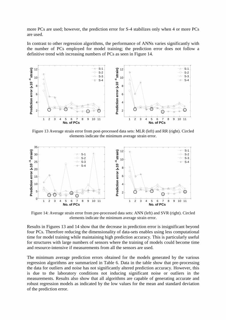
more PCs are used; however, the prediction error for S-4 stabilizes only when 4 or more PCs
are used.
In contrast to other regression algorithms, the performance of ANNs varies significantly with
the number of PCs employed for model training; the prediction error does not follow a
definitive trend with increasing numbers of PCs as seen in Figure 14.
Figure 13 Average strain error from post-processed data sets: MLR (left) and RR (right). Circled
elements indicate the minimum average strain error.
Figure 14: Average strain error from pre-processed data sets: ANN (left) and SVR (right). Circled
elements indicate the minimum average strain error.
Results in Figures 13 and 14 show that the decrease in prediction error is insignificant beyond
four PCs. Therefore reducing the dimensionality of data-sets enables using less computational
time for model training while maintaining high prediction accuracy. This is particularly useful
for structures with large numbers of sensors where the training of models could become time
and resource-intensive if measurements from all the sensors are used.
The minimum average prediction errors obtained for the models generated by the various
regression algorithms are summarized in Table 6. Data in the table show that pre-processing
the data for outliers and noise has not significantly altered prediction accuracy. However, this
is due to the laboratory conditions not inducing significant noise or outliers in the
measurements. Results also show that all algorithms are capable of generating accurate and
robust regression models as indicated by the low values for the mean and standard deviation
of the prediction error.
1 2 3 4 5 6 7 8 9 10 11
2
4
6
8
10
12
No. of PCs
Pre
dic
tio
n e
rro
r (
10
- 6
str
ain
)
S-1
S-2
S-3
S-4
1 2 3 4 5 6 7 8 9 10 11
2
4
6
8
10
12
No. of PCs
Pre
dic
tio
n e
rro
r (
10
- 6
str
ain
)
S-1
S-2
S-3
S-4
1 2 3 4 5 6 7 8 9 10 110
5
10
15
20
25
30
35
No. of PCs
Pre
dic
tio
n e
rro
r (
10
- 6
str
ain
)
S-1
S-2
S-3
S-4
1 2 3 4 5 6 7 8 9 10 11
2
4
6
8
10
12
No. of PCs
Pre
dic
tio
n e
rro
r (
10
- 6
str
ain
)
S-1
S-2
S-3
S-4

Figure 15: Predictions from a SVR model giving the response at sensor S-2 on the laboratory truss and
corresponding measured strains
Table 6: Prediction error (×10-6
strain) of regression models for data-sets from the laboratory truss
Algorithm S-1 S-2 S-3 S-4 Mean Standard deviation
MLR 2.30 1.98 2.22 1.83 2.08 0.22
MLR* 2.24 2.00 2.13 1.66 2.00 0.25
RR 2.37 2.16 2.31 1.71 2.14 0.30
RR* 2.29 2.16 2.19 1.54 2.05 0.35
ANN 3.17 2.52 2.16 2.66 2.63 0.42
ANN* 3.66 2.36 2.62 1.93 2.64 0.74
SVR 2.37 2.06 2.27 1.81 2.13 0.25
SVR* 2.30 2.14 2.12 1.59 2.04 0.31
*pre-processed for outliers and noise
6.1.2. The NPL footbridge
The data-sets collected from the NPL footbridge have a large number of samples due to the
high frequency of measurement collection. The time and resource requirements for generating
regression models, especially with algorithms of high levels of complexity (e.g., SVR, ANN),
increase significantly with the size of data-sets. This research therefore explores if reducing
the size of the training data-sets by reducing the frequency of measurement collection or, in
this case, simply ignoring measurements would speed up model generation with little loss in
prediction accuracy. The actual frequency of measurement collection (f) in the data-set is 3
measurements per hour. In this study, the frequency is artificially varied from 3 measurements
per hour to 1 measurement every 3 hours by regularly omitting measurements in the original
data-set. For this purpose, regression models are first generated for various sizes of the
training data-set and the performance of the models are then studied in terms of the average
prediction errors. While the size of the training sets are changed, the data-sets still present the
full variability in the measurements as only the number of input measurements is modified;
the duration of measurement collection is left unchanged.
The NPL footbridge, which is a concrete bridge, behaves differently to the previously-studied
aluminium truss, which due to its material properties immediately responds to changes in
ambient temperature. Concrete structures are more voluminous than metal structures; hence
3050 3100 3150 3200 3250 3300
-10
-5
0
5
10
15
20
25
Measurements
Str
ain
s (10
- 6
)
monitored
predicted

material temperature varies not only along the surface but also internally across the depth of
the sections of elements [39]. Due to its high thermal mass and low thermal conductivity,
internal temperatures within concrete elements may lag significantly behind the ambient
temperature. This phenomenon is often referred to as thermal inertia. Hua et al. [9] proposed a
“dynamic” approach to capture the effects of thermal inertia in their research investigating the
relationship between vibration modes and ambient temperatures. A similar approach is
adopted in this research. The input to the regression models is composed of both current (Di)
and former temperature (Di-j) measurements that have been transformed into PC space, i.e.
; i refers to the most recent measurement and j to a previous measurement set
collected j time-steps before i. From here onwards, j is referred to as the thermal inertia
parameter.
This sub-section therefore presents results from investigations on the influence of the
following features on prediction accuracy for regression algorithms:
(i) number of selected PCs;
(ii) number of input measurement (fi); and
(iii) thermal inertia parameter (j).
Figure 16 illustrates the variation of average prediction errors from regression models
generated using SVR for tilt sensors TL-1 and TL-2; prediction errors are plotted against the
number of PCs for different numbers of input measurements. Data-sets are pre-processed for
outliers and noise, and the thermal inertia parameter, j is equal to 1. In most cases, the
prediction error reduces as the number of inputs, i.e., the number of PCs, is increased. The
plots in Figure 16 show that the number of measurement inputs employed to train the
regression algorithm directly affects the prediction accuracy. While the prediction error
reduces with increasing frequency of measurement collection, the improvement in prediction
error is negligible when a sufficient number of PCs are used. For tilt sensors TL-1 and TL-2,
the prediction errors are small if 3 PCs and a measurement frequency of 1 measurement every
3 hours are specified (see Figure 16).
Next, the study analyses the influence of the thermal inertia parameter j on model
performance. Corresponding results, which are illustrated in Figure 17 and 18, show that there
is an optimal value for j for which the models have minimum prediction errors. In figure 17,
the variation of prediction errors with thermal inertia parameter j for tilt sensor TL-1 has a
sinusoidal pattern. Prediction errors reach their minimum when j = 36 and j = 108. The
periodicity of the pattern is therefore approximately 72 measurements, which is equivalent to
a time interval of one day. Figure 18 shows the variation of prediction errors with number of
PCs and the thermal inertia parameter j for each sensor. j is varied from 1 to 40; the prediction
error is minimum for j = 36. These results illustrate that the thermal response at any time-
instant is determined by the current set of temperature measurements and those collected 36
time-steps earlier. For the NPL footbridge, j = 36 corresponds to a time interval of half a day;
this value therefore suggests thermal lag in the structure caused by internal temperatures that
are closer to the ambient temperature taken 12 hours earlier in the day. Furthermore, the plots
also show that the thermal inertia parameter has a larger impact on the prediction errors for
sensors TL-1 and TL-4 than for TL-2 and TL-3. The reason for such behaviour may be due to
TL-1 and TL-4 being on the overhanging portions of the footbridge, which are much less
constrained to deform under thermal effects than its main-span.

Figure 16: Tilt prediction errors (mm/m) using SVR models for sensors TL-1 (left) and TL-2 (right).
Figure 17: Tilt prediction error (mm/m) versus number of PCs and thermal inertia parameter j from
sensor TL-1
The minimum tilt errors generated by the various regression algorithms for all tilt sensors are
given in Table 7. Results in the table show that pre-processing the measurements to manage
outliers and noise reduces prediction error by as much as 21%. Of the regression algorithms
studied, ANNs provide the minimum prediction errors for the NPL footbridge. Comparing
these results to those from the laboratory truss, we can conclude that the choice of the
regression algorithms used to model the temperature-response relationship is dependent on
the structure. The NPL footbridge is a concrete bridge. Changes in ambient temperature or
solar radiation are not immediately reflected in its response due to thermal inertia effects
arising from its low thermal conductivity and high thermal mass. The laboratory truss is made
of aluminium, a material with superior thermal conductivity, and therefore minimal thermal
inertia effects Furthermore, mechanical properties of concrete such as its elastic modulus are
also known to vary considerably with changes in temperature in comparison to aluminium.
Consequently, the nature of the relationship between temperatures and structural response for
the NPL footbridge and the laboratory truss are likely to be very different. Generalizing this,
the choice of regression model would be dependent on the structural system in consideration.
This is also in keeping with the well-known no-free-lunch theorem [40], which states that
there is no single algorithm that is optimal for all problem classes.
1 2 3 4 5 6 7 8 9 10
0.38
0.4
0.42
0.44
0.46
0.48
0.5
No. of PCs
Pre
dic
tio
n e
rro
r (m
m/m
)
f1
f10
f2 to f
9
1 2 3 4 5 6 7 8 9 10
0.02
0.022
0.024
0.026
0.028
0.03
No. of PCs
Pre
dic
tio
n e
rro
r (m
m/m
)
f1
f10
f2 to f
9

As noted in Table 7, the prediction errors observed for tilt sensors TL-2 and TL-3 are
significantly less than those for tilt sensors TL-1 and TL-4. This may be attributed to the fact
that measurements at TL-2 and TL-3 are more highly correlated with temperature
measurements than TL-1 and TL-4. However, the prediction errors are still not large in
magnitude when compared in terms of the range of measurements collected at these sensors
(see Table 4). TL-1 and TL-4 measure much larger tilts than TL-2 and TL-3 and therefore, the
normalized values of the errors are similar in magnitude. To illustrate this aspect, model
predictions and measurements at tilt sensors TL-1 and TL-2 are compared in Figures 19 and
20 respectively. For both sensors, model predictions closely follow actual measurements.
Figure 18: Tilt prediction error (mm/m) versus number of PCs and thermal inertia parameter j from
sensor TL-1 (top left), TL-2 (top right), TL-3 (bottom left) and TL-4 (bottom right).
Table 7: Average tilt error in mm/m
Algorithm TL-1 TL-2 TL-3 TL-4 Mean Standard deviation
MLR 0.273 0.026 0.036 0.236 0.143 0.130
MLR* 0.242 0.021 0.030 0.194 0.122 0.113
RR 0.271 0.026 0.036 0.235 0.142 0.129
RR* 0.240 0.020 0.029 0.193 0.121 0.112
ANN 0.225 0.022 0.030 0.195 0.118 0.107
ANN* 0.182 0.016 0.023 0.146 0.092 0.085
SVR 0.274 0.026 0.037 0.242 0.145 0.131
SVR* 0.237 0.020 0.029 0.192 0.120 0.111
*pre-processed

Figure 19: Predictions from a SVR model for tilt sensor TL-1 on the NPL footbridge and
corresponding measurements over a 9-day period.
Figure 20: Predictions from a SVR model for tilt sensor TL-2 on the NPL footbridge and
corresponding measurements over a 9-day period.
7. Summary and Conclusions
This paper proposes a data-driven strategy, referred to as Regression-Based Thermal
Response Prediction (RBTRP) methodology, for predicting thermal response of structures
from distributed temperature measurements. The main idea of the methodology is to develop
statistical regression models, which sufficiently capture the physical relationships between
structural response and temperature distributions, from distributed temperature and response
measurements collected during a reference period. This study investigates the application of
various statistical techniques such as MLR, RR, ANN and SVR for the generation of
regression models and then evaluates their performance on measurements taken from two
structures – a laboratory truss and a full-scale footbridge at the NPL.
This study has led to the following findings:
2700 2800 2900 3000 3100 3200-1.5
-1
-0.5
0
0.5
1
Measurements
Tilt
(mm
/m)
predicted
monitored
6100 6200 6300 6400 6500 6600 6700
0
0.1
0.2
0.3
0.4
Measurements
Tilt
(mm
/m)
predicted
monitored

The proposed RBTRP methodology leads to regression models that accurately predict
the thermal response of bridges from distributed temperature measurements.
All of the studied regression algorithms integrate effectively within the RBTRP
methodology. However, the optimal algorithm for a specific monitoring project is
determined by factors such as its structural properties and the quality of collected
measurements.
The number of samples employed for training regression models can be reduced
without greatly affecting the prediction accuracy. However the training data-set must
encompass the full range of variability in measurements. For a full-scale structure, this
implies that measurements covering at least one year may be required for training.
Using principal component analysis (PCA) to reduce the dimensionality of data-sets
given as input to the regression models does not significantly compromise prediction
accuracy.
Effects of thermal inertia are effectively modelled within the proposed methodology.
As seen from results for the NPL footbridge, this can be accomplished by providing
both current as well as previous temperature measurements as inputs to regression
models.
Future work will investigate embedding the proposed RBTRP methodology within an
anomaly detection strategy that examines the difference between thermal response predictions
and real-time measurements. Research will examine ways to cluster sensors prior to model
training to identify individual temperature measurements that are most relevant for predicting
response at specific locations. Thermal inertia effects will be studied in more depth to
evaluate if temperatures collected at several time-steps may be required to predict structural
response.
8. Acknowledgements
The authors would also like to thank Dr Elena Barton and the NPL for making measurements
and relevant information on the NPL footbridge available to this research. They would also
like to express their gratitude to Bill Harvey Associates and Pembrokeshire County Council
for providing access to the data from the Cleddau Bridge.
9. References
[1] Ni YQ, Zhou HF, Chan KC, Ko JM. Modal flexibility analysis of cable-stayed ting kau
bridge for damage identification. Computer-Aided Civil and Infrastructure Engineering.
2008;23:223-36.
[2] Inaudi D, Bolster M, Deblois R, French C, Phipps A, Sebasky J, et al. Structural health
monitoring system for the new i-35w st anthony falls bridge. Proceedings of 4th International
Conference on Structural Health Monitoring on Intelligent Infrastructure (SHMII-4). Zurich,
Switzerland; 2009.
[3] Brownjohn J. Structural health monitoring of civil infrastructure. Philos Transact A Math
Phys Eng Sci. . 2007;365:589–622.
[4] Aktan AE, Tsikos CJ, Catbas FN, Grimmelsman K, Barrish R. Challenges and
opportunities in bridge health monitoring. Proceedings of the 2nd International Workshop on
Structural Health Monitoring. Stanford, CA, USA, 1999.
[5] Bennet PJ, Stoianov I, Fidler P, Maksimovic C, Middletion C, Graham N, et al. Wireless
sensor networks: Creating 'smart infrastructure'. Proceedings of the ICE-Civil engineering:
Telford; 2009. p. 136-43.

[6] Fraser M, Elgamal A, He X, Conte JP. Sensor network for structural health monitoring of
a highway bridge. Journal of Computing in Civil Engineering. 2010;24:11-24.
[7] Lynch JP, Loh KJ. A summary review of wireless sensors and sensor networks for
structural health monitoring. Shock and Vibration Digest. 2006;38:91-130.
[8] Park G, Rosing T, Todd MD, Farrar CR, Hodgkiss W. Energy harvesting for structural
health monitoring sensor networks. Journal of Infrastructure Systems. 2008;14:64-79.
[9] Hua XG, Ni YQ, Ko JM, Wong KY. Modeling of temperature–frequency correlation
using combined principal component analysis and support vector regression technique.
Journal of Computing in Civil Engineering. 2007;21:122–35.
[10] Catbas FN, Susoy M, Frangopol DM. Structural health monitoring and reliability
estimation: Long span truss bridge application with environmental monitoring data
Engineering Structures. 2008;30:2347-59.
[11] Cross EJ, Koo KY, Brownjohn JMW, Worden K. Long-term monitoring and data
analysis of the tamar bridge. Mechanical Systems and Signal Processing. 2013;35:16-34.
[12] Ni YQ, Hu XG, Fan KQ, and Ko JM. Correlating modal properties with temperature
using long-term monitoring data and support vector machine technique. Engineering
Structures. 2005;27:P. 1762-73.
[13] Goulet JA, Kripakaran P, Smith IFC. Multimodel structural performance monitoring
Journal of Structural Engineering. 2010;136:1309-18.
[14] Posenato D, Kripakaran P, Inaudi D, Smith IFC. Methodologies for model-free data
interpretation of civil engineering structures. Computers and Structures. 2010;88:467-82.
[15] Moyo P, Brownjohn J. Detection of anomalous structural behaviour using wavelet
analysis. Mechanical Systems and Signal Processing. 2002;16:429-45.
[16] Omenzetter P, Brownjohn JMW. Application of time series analysis for bridge
monitoring. Smart Materials and Structures. 2006;15:129.
[17] Laory I, Ali NBH, Trinh TN, Smith IFC. Measurement system configuration for damage
identification of continuously monitored structures. Journal of Bridge Engineering.
2012;17:NA.
[18] Potgieter IC, Gamble WL. Nonlinear temperature distributions in bridges at different
locations in the united states. PCI Journal. 1989;July-August 1989:80-103.
[19] Li ZX, Chanb THT, Zheng R. Statistical analysis of online strain response and its
application in fatigue assessment of a long-span steel bridge Engineering Structures.
2003;25:1731–41.
[20] Mata J, Castro ATd, Costa JSd. Time–frequency analysis for concrete dam safety
control: Correlation between the daily variation of structural response and air temperature.
Engineering Structures. 2013;48:658-65.
[21] Laory I, Trinh TN, Posenato D, Smith IFC. Combined model-free data-interpretation
methodologies for damage detection during continuous monitoring of structures. Journal of
Computing in Civil Engineering. 2013.
[22] Mehrjoo M, Khaji N, Moharrami H, Bahreininejad A. Damage detection of truss bridge
joints using artificial neural networks. Expert Systems with Applications. 2008;35:1122-31.
[23] Ko J, Sun Z, Ni Y. Multi-stage identification scheme for detecting damage in cable-
stayed kap shui mun bridge. Engineering Structures. 2002;24:857-68.
[24] Zhang J, Sato T, Iai S. Support vector regression for on-line health monitoring of large-
scale structures. Structural Safety. 2006;28:392-406.
[25] Kromanis R, Kripakaran P. Support vector regression for anomaly detection from
measurement histories. Advanced Engineering Informatics. 2013;27:486–95.
[26] Aiken LS, West SG, Pitts SC. Multiple linear regression. In: Schinka JA, Velicer WF,
editors. Handbook of psychology. Volume 2: Research methods in psychology. Hoboken,
New Jersey: John Wiley & Sons, Inc.; 2003. p. 484-507.

[27] Huber PJ. Robust regression: Asymptotics, conjectures and monte carlo. The Annals of
Statistics. 1973;1:799-821.
[28] Basheer IA, Hajmeer M. Artificial neural networks: Fundamentals, computing, design,
and application. Journal of Microbiological Methods. 2000;43:3-31.
[29] MATLAB. And statistics toolbox release 2011b. The MathWorks, Inc., Natick,
Massachusetts, United States.
[30] Dackermann U. Vibration-based damage identification methods for civil engineering
structures using artificial neural networks [Dissertation]. Sydney: University of Technology
Sydney; 2010.
[31] Mata J. Interpretation of concrete dam behaviour with artificial neural network and
multiple linear regression models. Engineering Structures. 2011;33:903-10.
[32] Katsikeros CE, Labeas G. Development and validation of a strain-based structural health
monitoring system. Mechanical Systems and Signal Processing. 2009;23:372-83.
[33] Haykin SS. Neural networks: A comprehensive foundation: Prentice Hall; 1999.
[34] Vapnik VN. The nature of statistical learning theroy. 2nd edition. New York: Springer-
Verlag New York Inc.; 1999.
[35] Smola AJ, Schölkopf B. A tutorial on support vector regression. Statistics and
Computing. 2004;14:199-222.
[36] Kotsiantis SB, Kanellopoulos D, Pintelas PE. Data preprocessing for supervised learning
International Journal of Computers Sciences. 2006;1:111-7.
[37] Ganguli R. Noise and outlier removal from jet engine health signals using weighted fir
median hybrid filters. Mechanical Systems and Signal Processing. 2002;16:967-78.
[38] Jolliffe IT. Principal component analysis. 2nd Ed., Springer-Verlag, Inc., New York.
2002.
[39] Branco FA, Mendes PA. Thermal actions for concrete bridge design. Journal of
Structural Engineering. 1993;119:2313-31.
[40] Wolpert DH, Macready WG. No free lunch theorems for optimization. Evolutionary
Computation, IEEE Transactions on. 1997;1:67-82.