Embed Size (px)
Citation preview
1
Predictionand
ResourceAllocation
By Thomas Saaty
Predictionand
ResourceAllocation
By Thomas Saaty
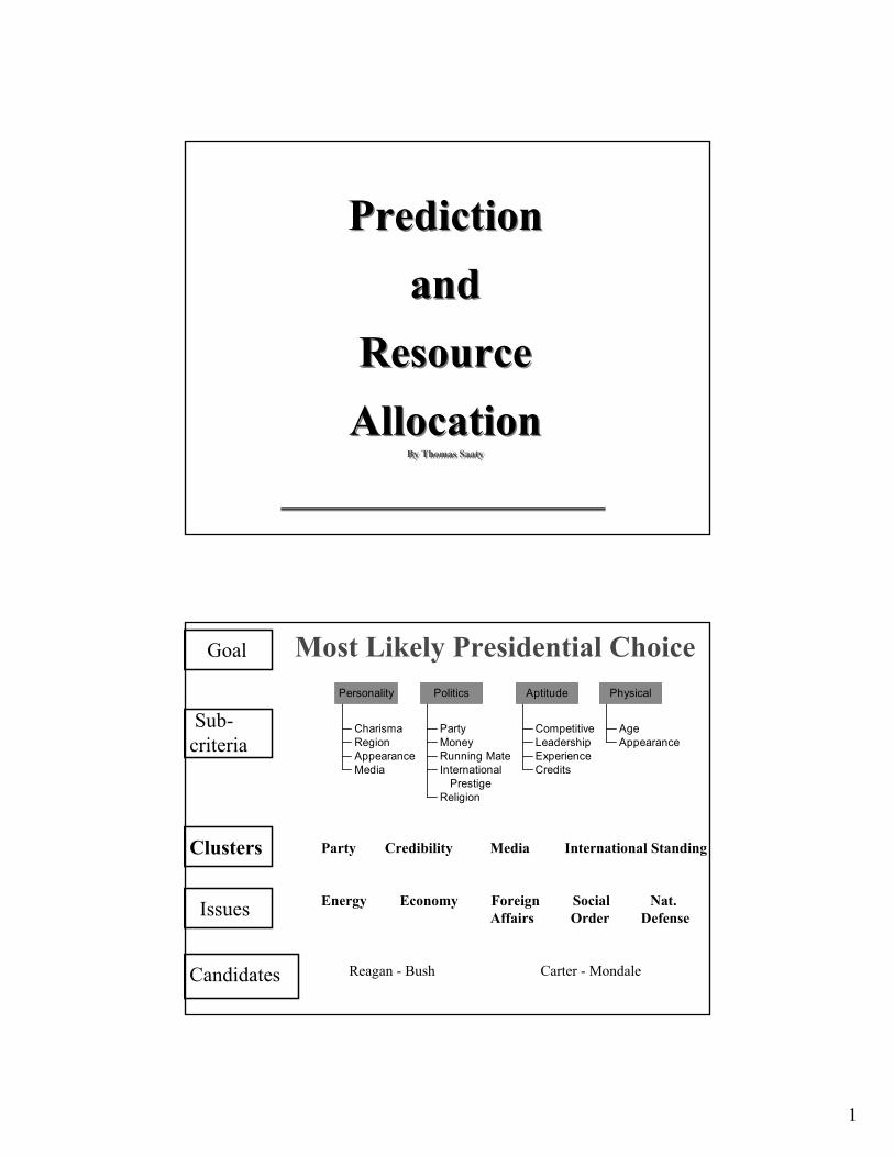
Most Likely Presidential Choice
CharismaRegionAppearanceMedia
Personality
PartyMoneyRunning MateInternational
PrestigeReligion
Politics
CompetitiveLeadershipExperienceCredits
Aptitude
AgeAppearance
Physical
Party Credibility Media International Standing
Energy Economy Foreign Social Nat. Affairs Order Defense
Reagan - Bush Carter - Mondale
Clusters
Issues
Candidates
Sub-criteria
Goal
2
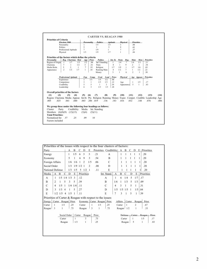
CARTER VS. REAGAN 1980Priorities of Criteria
Election 1980 Personality Politics Aptitude Physical PrioritiesPersonality 1 1/5 1/5 3 .08Politics 5 1 5 9 .61Professional Aptitude 7 1/9 1 7 .27Physical 1/3 1/9 1/7 1 .04
Priorities of the factors which define the criteriaPersonality Reg. Charisma Med App Prior. Politics Int. St. Party Reg. Mate Mon PrioritiesRegion of Origin 1 1/7 1/5 1/2 .06 Int’l Standing 1 1/4 7 1/4 1/3 .11Charisma 7 1 1/2 3 .32 Party 4 1 9 2 1 .34Media Relat. 5 2 1 7 .52 Religion 1/7 1/9 1 1/7 1/6 .03Appearance 2 1/3 1/7 1 .10 Running Mate 4 1/2 7 1 1/2 .22
Money 3 1 6 2 1 .30
Professional Aptitude Exp. Comp. Cred. Lead Prior. Physical Age Appear. PrioritiesExperience 1 1/3 1/5 1/2 .06 Competence 3 1 1/5 1/3 .12 Age 1 1/5 .17Credibility 5 5 1 3 .54 Appearance 5 1 .83Leadership 6 3 1/3 1/3 .28
Overall priorities of the factors(1) (2) (3) (4) (5) (6) (7) (8) (9) (10) (11) (12) (13) (14)
Region Charisma Media Appear. Int.St. Pty. Religion Running Money Exper. Compet. Credible Leadership Age.005 .025 .041 .040 .065 .206 .019 .136 .183 .016 .032 .148 .076 .006
We group these under the following four headings as follows:Cluster Party Credibility Media Int. StandingMembers (6)(8)(9) (12)(13) (3)(4) (5)(11)Total Priorities:Normalized for .57 .25 .09 10Factors included
Priorities of the issues with respect to the four clusters of factors:Party A B C D E Prioirites Credibility A B C D E PrioritiesEnergy 1 1/5 6 3 3 .21 A 1 1 1 1 1 .20Economy 5 1 6 9 3 .54 B 1 1 1 1 1 .20Foreign Affairs 1/6 1/6 1 2 1/5 .06 C 1 1 1 1 1 .20Social Order 1/3 1/9 1/2 1 2 .08 D 1 1 1 1 1 .20National Defense 1/3 1/5 5 1/2 1 .11 E 1 1 1 1 1 .20Media A B C D E Priorities Int. Stand. A B C D E Priorities
A 1 1/5 1/4 1/3 3 .12 A 1 6 1/4 5 1/7 .17B 2 1 5 3 5 .39 B 1/6 1 1/3 5 1/3 .09C 4 1/5 1 1/4 1/4 .11 C 4 3 1 5 1 .31D 3 1/3 4 1 5 .27 D 1/5 1/5 1/5 1 1/5 .04E 1/2 1/5 4 1/5 1 .11 E 7 3 1 5 1 .39
Priorities of Carter & Reagan with respect to the issues:Energy Carter Reagan Prior. Economy Carter Reagan Prior. Affairs Carter Reagan Prior.Carter 1 1/3 .25 Carter 1 1/3 .25 Carter 1 2 .67Reagan 3 1 .75 Reagan 3 1 .75 Reagan 1/2 1 .33
Social Order Carter Reagan Prior. Defense Carter Reagan Prior. Carter 1 3 .75 Carter 1 1/5 .17Reagan 1/3 1 .25 Reagan 5 1 .83
3
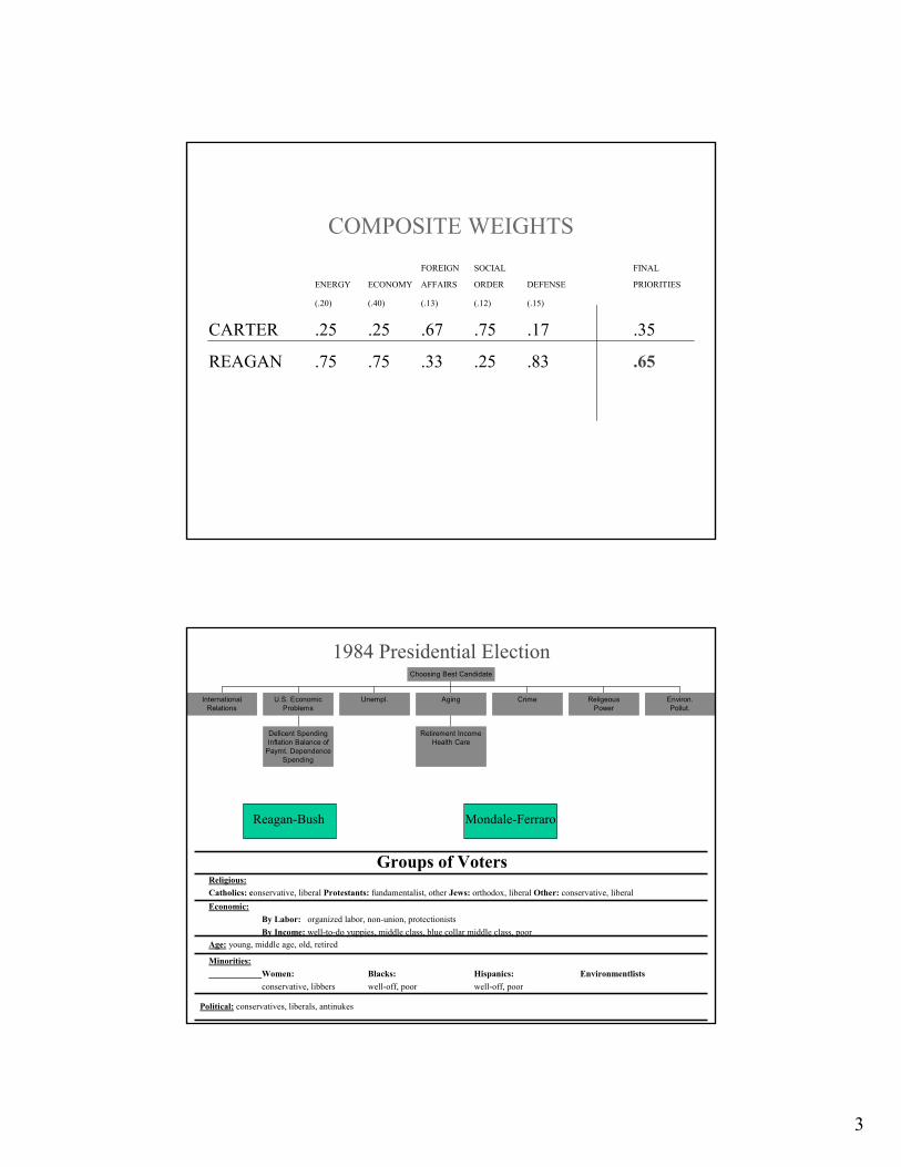
COMPOSITE WEIGHTSFOREIGN SOCIAL FINAL
ENERGY ECONOMY AFFAIRS ORDER DEFENSE PRIORITIES
(.20) (.40) (.13) (.12) (.15)
CARTER .25 .25 .67 .75 .17 .35
REAGAN .75 .75 .33 .25 .83 .65
InternationalRelations
Deficent SpendingInflation Balance of
Paymt. DependenceSpending
U.S. EconomicProblems
Unempl.
Retirement IncomeHealth Care
Aging Crime ReligeousPower
Environ.Pollut.
Choosing Best Candidate
Reagan-Bush Mondale-Ferraro
1984 Presidential Election
Groups of Voters Religious:Catholics: conservative, liberal Protestants: fundamentalist, other Jews: orthodox, liberal Other: conservative, liberalEconomic:
By Labor: organized labor, non-union, protectionistsBy Income: well-to-do yuppies, middle class, blue collar middle class, poor
Age: young, middle age, old, retired
Minorities:Women: Blacks: Hispanics: Environmentlistsconservative, libbers well-off, poor well-off, poor
Political: conservatives, liberals, antinukes
4
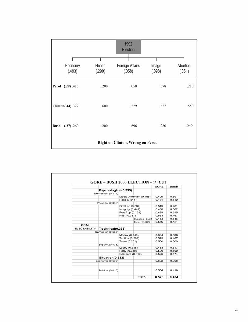
Economy(.493)
Health(.299)
Foreign Affairs(.058)
Image(.098)
Abortion(.051)
1992Election
Perot (.29)
Clinton(.44)
Bush (.27)
.413 .200 .058 .098 .210
.327 .600 .229 .627 .550
.260 .200 .696 .280 .249
Right on Clinton, Wrong on Perot
GORE BUSHPsychological(0.333)
Momentum (0.114)Media Attention (0.455) 0.409 0.591Polls (0.544) 0.481 0.519
Personal (0.886)FirstLad (0.094) 0.519 0.481Integrity (0.441) 0.438 0.562PersApp (0.133) 0.485 0.515Past (0.331) 0.533 0.467
Success (0.533 0.453 0.546Exper. (0.467) 0.576 0.424
GOALELECTABILITY Technical(0.333)
Campaign (0.562)Money (0.440) 0.394 0.606Tactics (0.299) 0.513 0.487Team (0.261) 0.500 0.500
Support (0.438)Lobby (0.348) 0.483 0.517Party (0.340) 0.500 0.500Contacts (0.312) 0.526 0.474
Situation(0.333) Economic (0.590) 0.692 0.308
Political (0.410) 0.584 0.416
TOTAL 0.526 0.474
GORE – BUSH 2000 ELECTION – 1ST CUT
5
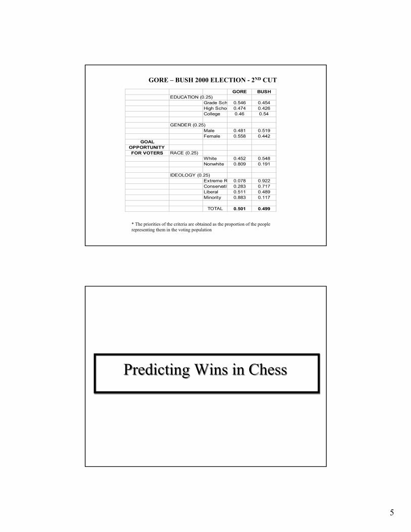
GORE – BUSH 2000 ELECTION - 2ND CUTGORE BUSH
EDUCATION (0.25)Grade Sch 0.546 0.454High Schoo 0.474 0.426College 0.46 0.54
GENDER (0.25)Male 0.481 0.519Female 0.558 0.442
GOALOPPORTUNITY FOR VOTERS RACE (0.25)
White 0.452 0.548Nonwhite 0.809 0.191
IDEOLOGY (0.25)Extreme R 0.078 0.922Conservativ 0.283 0.717Liberal 0.511 0.489Minority 0.883 0.117
TOTAL 0.501 0.499
* The priorities of the criteria are obtained as the proportion of the people representing them in the voting population
Predicting Wins in ChessPredicting Wins in Chess
6
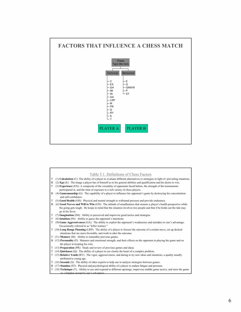
CEXGHIMINGALRPMPRQRYST
Technical
EGGNWWPST
Behavioral
ChessType title here
PLAYER A PLAYER B
FACTORS THAT INFLUENCE A CHESS MATCH
Table 5.1. Definitions of Chess FactorsT (1) Calculation (C): The ability of a player to evaluate different alternatives or strategies in light of prevailing situations.B (2) Ego (E): The image a player has of himself as to his general abilities and qualification and his desire to win.T (3) Experience (EX): A composite of the versatility of opponents faced before, the strength of the tournaments
participated in, and the time of exposure to a rich variety of chess players.B (4) Gamesmanship (G): The capability of a player to influence his opponent’s game by destroying his concentration
and self-confidence.T (5) Good Health (GH): Physical and mental strength to withstand pressure and provide endurance.B (6) Good Nerves and Will to Win (GN): The attitude of steadfastness that ensures a player’s health perspective while
the going gets tough. He keeps in mind that the situation involves two people and that if he holds out the tide maygo in his favor.
T (7) Imagination (IM): Ability to perceived and improvise good tactics and strategiesT (8) Intuition (IN): Ability to guess the opponent’s intentions.T (9) Game Aggressiveness (GA): The ability to exploit the opponent’s weaknesses and mistakes to one’s advantage.
Occasionally referred to as “killer instinct.”T (10) Long Range Planning (LRP): The ability of a player to foresee the outcome of a certain move, set up desired
situations that are more favorable, and work to alter the outcome.T (11) Memory (M): Ability to remember previous games.B (12) Personality (P): Manners and emotional strength, and their effects on the opponent in playing the game and on
the player in keeping his wits.T (13) Preparation (PR): Study and review of previous games and ideas.T (14) Quickness (Q): The ability of a player to see clearly the heart of a complex problem.T (15) Relative Youth (RY): The vigor, aggressiveness, and daring to try new ideas and situations, a quality usually
attributed to young age.T (16) Seconds (S): The ability of other experts to help one to analyze strategies between games.B (17) Stamina (ST): Physical and psychological ability of a player to endure fatigue and pressure.T (18) Technique (T): Ability to use and respond to different openings, improvise middle game tactics, and steer the game
to a familiar ground to one’s advantage.
7
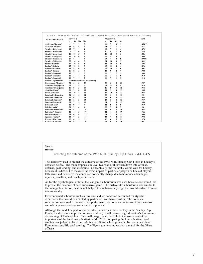
TABLE 5.7. ACTUAL AND PREDICTED OUTCOME OF WORLD CHESS CHAMPIONSHIP MATCHES (1858-1981)OUTCOME PREDICTION YEARn NA NB ND n NA NB ND
Anderson-Morphy* 11 7 2 2 11 7 3 1 1858-59Anderson-Steinitz* 14 8 6 0 14 7 6 1 1866Steinitz*-Zukertort 12 7 1 4 12 7 1 4 1872Steinitz*-Blackburn 7 7 0 0 6 5 1 0 1876Steinitz*-Zukertort 20 10 5 5 21 10 5 6 1886Steinitz*-Tchigorin 17 10 6 1 17 9 6 2 1889Steinitz*-Gunsberg 19 6 4 9 19 7 4 8 1890-91Steinitz*-Tchigorin 23 10 8 5 24 10 9 5 1892Steinitz-Lasker* 19 10 5 4 20 10 5 5 1894Lasker*-Steinitz 17 10 2 5 19 11 4 4 1896Lasker*-Marshall 15 8 0 7 17 10 1 6 1907Lasker*-Tarash 16 8 3 5 20 9 4 7 1908Lasker*-Janowski 10 7 1 2 11 7 2 2 1909Lasker*-Schlecter 10 1 1 8 11 1 1 9 1910Lasker*-Janowski 10 7 1 2 11 7 1 3 1910Lasker-Capablanca* Match discontiued prematurelyCapablanca-Alekhine* 34 6 3 25 35 6 4 25 1927Alekhine*-Bogoljubov 25 11 5 9 25 11 5 9 1929Alekhine*-Bogoljubov 26 8 3 15 26 8 3 15 1934Alekhine-Euwe* 30 9 8 13 30 9 8 13 1935Euwe-Alekhine* 25 10 4 11 25 10 4 11 1937Botvinnik*-Bronstein 24 5 5 14 25 5 5 15 1951Botvinnik*-Smyslov 22 6 3 13 23 6 4 13 1954Botvinnik-Smyslov* 21 6 2 13 23 6 4 13 1957Smyslov-Botvinnik* 23 7 5 11 24 7 5 12 1958Botvinnik-Tal* 21 9 4 8 22 9 4 9 1960Tal-Botvinnik* 21 9 4 8 22 9 4 9 1961Botvinnik-Petrosian* 23 5 3 15 23 5 3 15 1963Petrosian*-Spassky 24 4 3 17 24 4 3 17 1966Petrosian-Spassky* 23 6 4 13 23 7 4 12 1969Spassky-Fischer* 21 7 3 11 20 7 2 11 1972Karpov*-Korchnoi 32 6 5 21 32 6 5 21 1978Karpov*-Korchnoi 18 6 2 10 18 6 2 10 1981
*WINNER OF MATCH
SportsHockey
Predicting the outcome of the 1985 NHL Stanley Cup Finals. ( slide 1 of 2)
The hierarchy used to predict the outcome of the 1985 NHL Stanley Cup Finals in hockey is depicted below. The main emphasis in level two was skill, broken down into offense, defense, goal tending, and discipline. Conceptually, the hierarchy works well for hockey, because it is difficult to measure the exact impact of particular players or lines of players. Offensive and defensive matchups can constantly change due to home-ice advantages, injuries, penalties, and coach preferences.As for the psychological criteria, the last game subcriterion was used because one would like to predict the outcome of each successive game. The dislike/like subcriterion was similar to the intangible criterion, heat, which helped to emphasize any edge that would surface from an intense rivalry.Environmental subcritera such as rink size and ice condition accounted for stylistic differences that would be affected by particular rink characteristics. The home ice subcriterion was used to consider past performance on home ice, in terms of both win-lose records in general and against a specific opponent.Although the model helped to successfully predict the Oilers’ victory in the Stanley Cup Finals, the difference in prediction was relatively small considering Edmonton’s four to one dispatching of Philadelphia. The small margin is attributable to the assessment of the importance of the level two subcriterion “skill”. In comparing the four subcritera, goal tending was judged to be strong relative to offense, which proved to be inaccurate given Edmonton’s prolific goal scoring. The Flyers goal tending was not a match for the Oilersoffense.
8
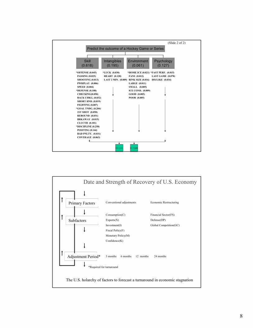
Skill(0.618)
Intangibles(0.195)
Environment(0.061)
Psychology(0.127)
Predict the outcome of a Hockey Game or Series
(Slide 2 of 2)
*OFFENSE (0.045)PASSING (0.025)SHOOTING (0.013)PWRPLAY (0.006)SPEED (0.004)
*DEFENSE (0.108)CHECKING(0.050)BACK CHKG. (0.032)SHORT HND. (0.019)FIGHTING (0.007)
*GOAL TNDG. (0.204)1ST SHOT (0.058)REBOUND (0.031)BRKAWAY (0.015)CLUCTH (0.101)
*DISCIPLINE (0.258)POSITING (0.144)BAD PNLTY. (0.031)COVERAGE (0.063)
*LUCK (0.030)HEART (0.128)LAST 2 MIN. (0.009)
*HOME ICE (0.021)FANS (0.012)RINK SIZE (0.016)LARGE (0.011)SMALL (0.005)ICE COND. (0.009)GOOD (0.005)POOR (0.005)
*FAST PERF. (0.015)LAST GAME (0.078)DIS/LIKE (0.034)
OILERS FLYERS
Primary Factors
Subfactors
Adjustment Period*
*Required for turnaround
Conventional adjustments Economic Restructuring
Consumption(C) Financial Sector(FS)
Exports(X) Defense(DP)
Investment(I) Global Competition(GC)
Fiscal Policy(F)
Monetary Policy(M)
Confidence(K)
3 months 6 months 12 months 24 months
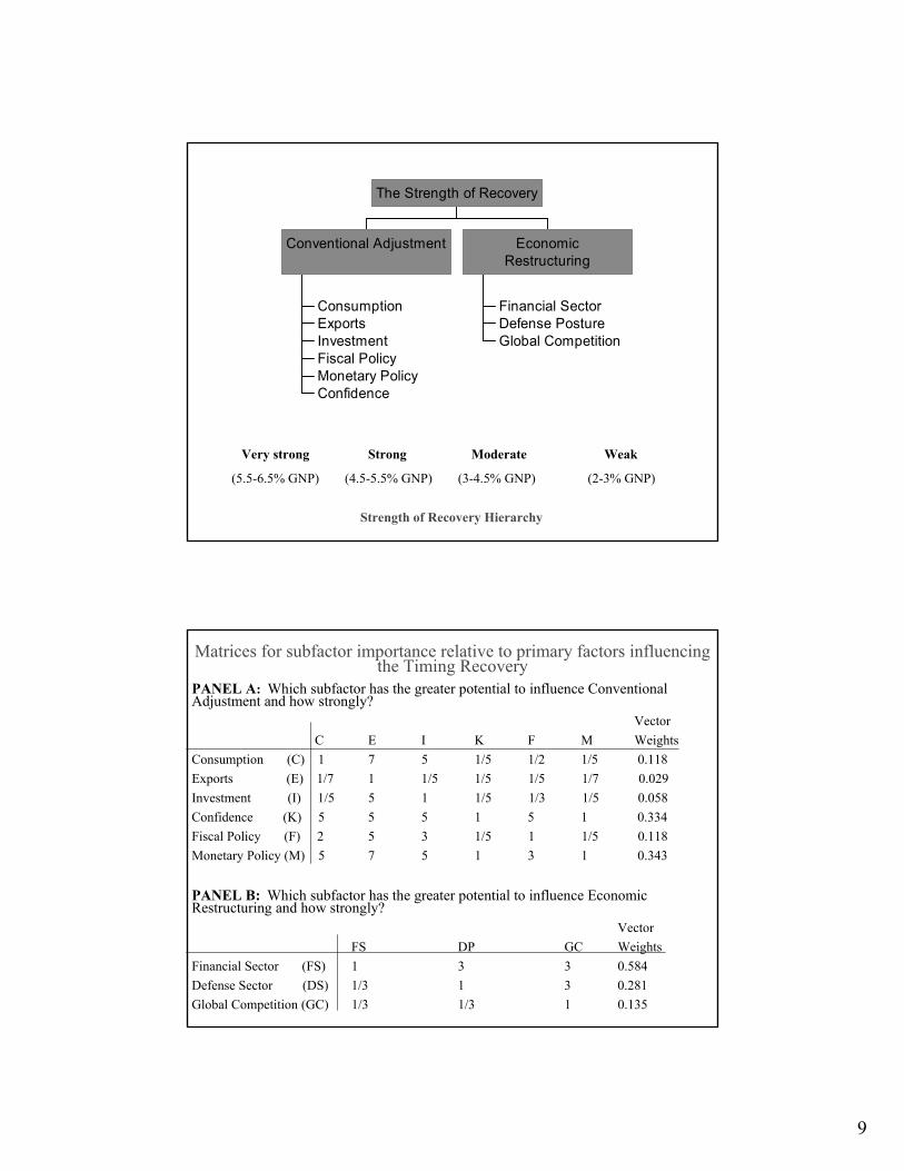
The U.S. holarchy of factors to forecast a turnaround in economic stagnation
Date and Strength of Recovery of U.S. Economy
9
ConsumptionExportsInvestmentFiscal PolicyMonetary PolicyConfidence
Conventional Adjustment
Financial SectorDefense PostureGlobal Competition
EconomicRestructuring
The Strength of Recovery
Very strong Strong Moderate Weak
(5.5-6.5% GNP) (4.5-5.5% GNP) (3-4.5% GNP) (2-3% GNP)
Strength of Recovery Hierarchy
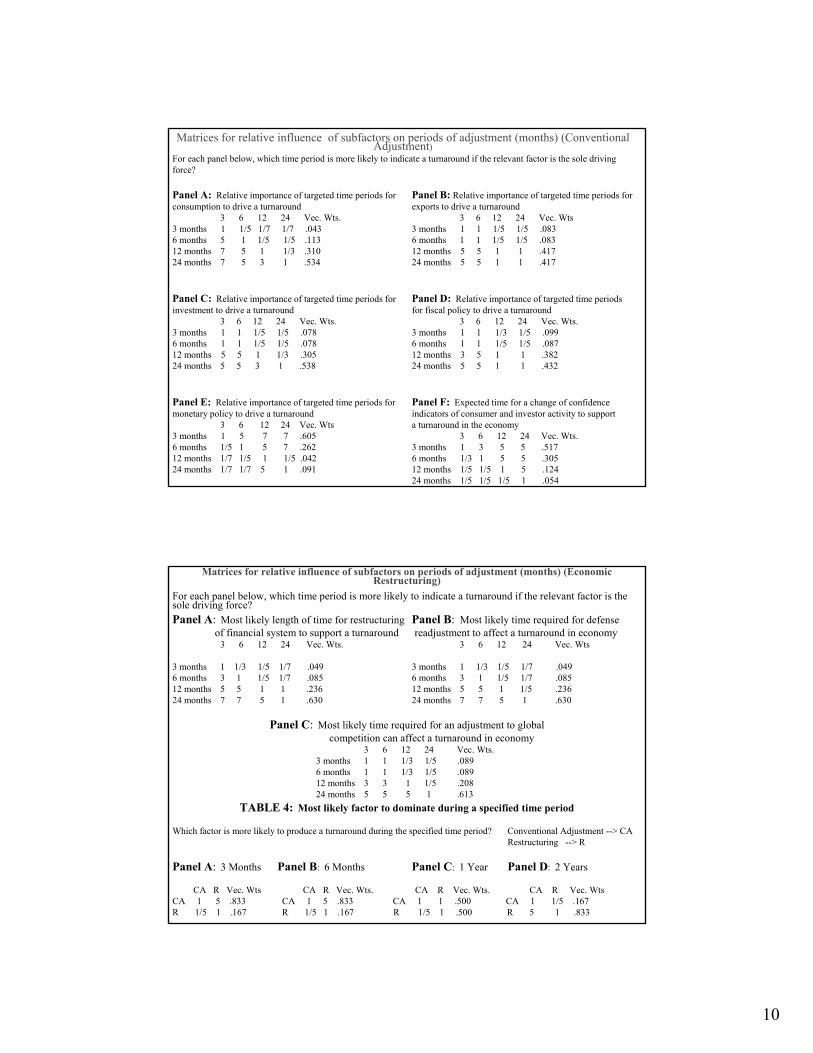
Matrices for subfactor importance relative to primary factors influencing the Timing Recovery
PANEL A: Which subfactor has the greater potential to influence Conventional Adjustment and how strongly?
VectorC E I K F M Weights
Consumption (C) 1 7 5 1/5 1/2 1/5 0.118Exports (E) 1/7 1 1/5 1/5 1/5 1/7 0.029Investment (I) 1/5 5 1 1/5 1/3 1/5 0.058Confidence (K) 5 5 5 1 5 1 0.334 Fiscal Policy (F) 2 5 3 1/5 1 1/5 0.118Monetary Policy (M) 5 7 5 1 3 1 0.343
PANEL B: Which subfactor has the greater potential to influence Economic Restructuring and how strongly?
VectorFS DP GC Weights
Financial Sector (FS) 1 3 3 0.584Defense Sector (DS) 1/3 1 3 0.281Global Competition (GC) 1/3 1/3 1 0.135
10
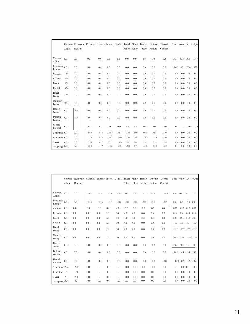
Matrices for relative influence of subfactors on periods of adjustment (months) (Conventional Adjustment)
For each panel below, which time period is more likely to indicate a turnaround if the relevant factor is the sole driving force?
Panel A: Relative importance of targeted time periods for Panel B: Relative importance of targeted time periods for consumption to drive a turnaround exports to drive a turnaround
3 6 12 24 Vec. Wts. 3 6 12 24 Vec. Wts3 months 1 1/5 1/7 1/7 .043 3 months 1 1 1/5 1/5 .0836 months 5 1 1/5 1/5 .113 6 months 1 1 1/5 1/5 .08312 months 7 5 1 1/3 .310 12 months 5 5 1 1 .41724 months 7 5 3 1 .534 24 months 5 5 1 1 .417
Panel C: Relative importance of targeted time periods for Panel D: Relative importance of targeted time periods investment to drive a turnaround for fiscal policy to drive a turnaround
3 6 12 24 Vec. Wts. 3 6 12 24 Vec. Wts.3 months 1 1 1/5 1/5 .078 3 months 1 1 1/3 1/5 .0996 months 1 1 1/5 1/5 .078 6 months 1 1 1/5 1/5 .08712 months 5 5 1 1/3 .305 12 months 3 5 1 1 .38224 months 5 5 3 1 .538 24 months 5 5 1 1 .432
Panel E: Relative importance of targeted time periods for Panel F: Expected time for a change of confidence monetary policy to drive a turnaround indicators of consumer and investor activity to support
3 6 12 24 Vec. Wts a turnaround in the economy3 months 1 5 7 7 .605 3 6 12 24 Vec. Wts.6 months 1/5 1 5 7 .262 3 months 1 3 5 5 .51712 months 1/7 1/5 1 1/5 .042 6 months 1/3 1 5 5 .30524 months 1/7 1/7 5 1 .091 12 months 1/5 1/5 1 5 .124
24 months 1/5 1/5 1/5 1 .054
Matrices for relative influence of subfactors on periods of adjustment (months) (Economic Restructuring)
For each panel below, which time period is more likely to indicate a turnaround if the relevant factor is the sole driving force?Panel A: Most likely length of time for restructuring Panel B: Most likely time required for defense
of financial system to support a turnaround readjustment to affect a turnaround in economy3 6 12 24 Vec. Wts. 3 6 12 24 Vec. Wts
3 months 1 1/3 1/5 1/7 .049 3 months 1 1/3 1/5 1/7 .0496 months 3 1 1/5 1/7 .085 6 months 3 1 1/5 1/7 .08512 months 5 5 1 1 .236 12 months 5 5 1 1/5 .23624 months 7 7 5 1 .630 24 months 7 7 5 1 .630
Panel C: Most likely time required for an adjustment to globalcompetition can affect a turnaround in economy
3 6 12 24 Vec. Wts.3 months 1 1 1/3 1/5 .0896 months 1 1 1/3 1/5 .08912 months 3 3 1 1/5 .20824 months 5 5 5 1 .613
TABLE 4: Most likely factor to dominate during a specified time period
Which factor is more likely to produce a turnaround during the specified time period? Conventional Adjustment --> CARestructuring --> R
Panel A: 3 Months Panel B: 6 Months Panel C: 1 Year Panel D: 2 Years
CA R Vec. Wts CA R Vec. Wts. CA R Vec. Wts. CA R Vec. WtsCA 1 5 .833 CA 1 5 .833 CA 1 1 .500 CA 1 1/5 .167R 1/5 1 .167 R 1/5 1 .167 R 1/5 1 .500 R 5 1 .833
11
Conven- Economic Consum. Exports Invest. Confid. Fiscal Monet Financ. Defense Global 3 mo. 6mo. 1yr. >=2yrs
Adjust Restruc. Policy Policy Sector Posture Compet
ConvenAdjust
Economic Restruc.
Consum
Exports
Invest
Confid
Fiscal Policy
Monetary Policy
Financ. Sector
Defense Posture
Global Compet.
3 monthes
6 monthes
1 year
>= 2 years
0.0 0.0 0.0 0.0 0.0 0.0 0.0 0.0 0.0 0.0 0.0 .833 .833 .500 .167
0.0 0.0 0.0 0.0 0.0 0.0 0.0 0.0 0.0 0.0 0.0 .167 .167 .500 .833
.118 0.0 0.0 0.0 0.0 0.0 0.0 0.0 0.0 0.0 0.0 0.0 0.0 0.0 0.0
.029 0.0 0.0 0.0 0.0 0.0 0.0 0.0 0.0 0.0 0.0 0.0 0.0 0.0 0.0
0.0 0.0 .310 .417 .305 .124 .383 .042 .236 .236 .209 0.0 0.0 0.0 0.0
.334 0.0 0.0 0.0 0.0 0.0 0.0 0.0 0.0 0.0 0.0 0.0 0.0 0.0 0.0
.118 0.0 0.0 0.0 0.0 0.0 0.0 0.0 0.0 0.0 0.0 0.0 0.0 0.0 0.0
.343 0.0 0.0 0.0 0.0 0.0 0.0 0.0 0.0 0.0 0.0 0.0 0.0 0.0 0.0
0.0 .584 0.0 0.0 0.0 0.0 0.0 0.0 0.0 0.0 0.0 0.0 0.0 0.0 0.0
0.0 .584 0.0 0.0 0.0 0.0 0.0 0.0 0.0 0.0 0.0 0.0 0.0 0.0 0.0
0.0 .135 0.0 0.0 0.0 0.0 0.0 0.0 0.0 0.0 0.0 0.0 0.0 0.0 0.0
0.0 0.0 .043 .083 .078 .517 .099 .605 .049 .049 .089 0.0 0.0 0.0 0.0
0.0 0.0 .113 .083 .078 .305 .086 .262 .085 .085 .089 0.0 0.0 0.0 0.0
.058 0.0 0.0 0.0 0.0 0.0 0.0 0.0 0.0 0.0 0.0 0.0 0.0 0.0 0.0
0.0 0.0 .534 .417 .539 .054 .432 .091 .630 .630 .613 0.0 0.0 0.0 0.0
Conven- Economic Consum. Exports Invest. Confid. Fiscal Monet Financ. Defense Global 3 mo. 6mo. 1yr. >=2yrs
Adjust Restruc. Policy Policy Sector Posture Compet
ConvenAdjust
Economic Restruc.
Consum
Exports
Invest
Confid
Fiscal Policy
Monetary Policy
Financ. Sector
Defense Posture
Global Compet.
3 monthes
6 monthes
1 year
>= 2 years
0.0 0.0 .484 .484 .484 .484 .484 .484 .484 .484 .484 0.0 0.0 0.0 0.0
0.0 0.0 .516 .516 .516 .516 .516 .516 .516 .516 .513 0.0 0.0 0.0 0.0
0.0 0.0 0.0 0.0 0.0 0.0 0.0 0.0 0.0 0.0 0.0 .057 .057 .057 .057
0.0 0.0 0.0 0.0 0.0 0.0 0.0 0.0 0.0 0.0 0.0 .014 .014 .014 .014
.201 .201 0.0 0.0 0.0 0.0 0.0 0.0 0.0 0.0 0.0 0.0 0.0 0.0 0.0
0.0 0.0 0.0 0.0 0.0 0.0 0.0 0.0 0.0 0.0 0.0 .162 .162 .162 .162
0.0 0.0 0.0 0.0 0.0 0.0 0.0 0.0 0.0 0.0 0.0 .057 .057 .057 .057
0.0 0.0 0.0 0.0 0.0 0.0 0.0 0.0 0.0 0.0 0.0 .166 .166 .166 .166
0.0 0.0 0.0 0.0 0.0 0.0 0.0 0.0 0.0 0.0 0.0 .301 .301 .301 .301
0.0 0.0 0.0 0.0 0.0 0.0 0.0 0.0 0.0 0.0 0.0 .145 .145 .145 .145
0.0 0.0 0.0 0.0 0.0 0.0 0.0 0.0 0.0 0.0 0.0 .070 .070 .070 .070
.224 .224 0.0 0.0 0.0 0.0 0.0 0.0 0.0 0.0 0.0 0.0 0.0 0.0 0.0
.151 .151 0.0 0.0 0.0 0.0 0.0 0.0 0.0 0.0 0.0 0.0 0.0 0.0 0.0
0.0 0.0 0.0 0.0 0.0 0.0 0.0 0.0 0.0 0.0 0.0 .028 .028 .028 .028
.424 .424 0.0 0.0 0.0 0.0 0.0 0.0 0.0 0.0 0.0 0.0 0.0 0.0 0.0
12
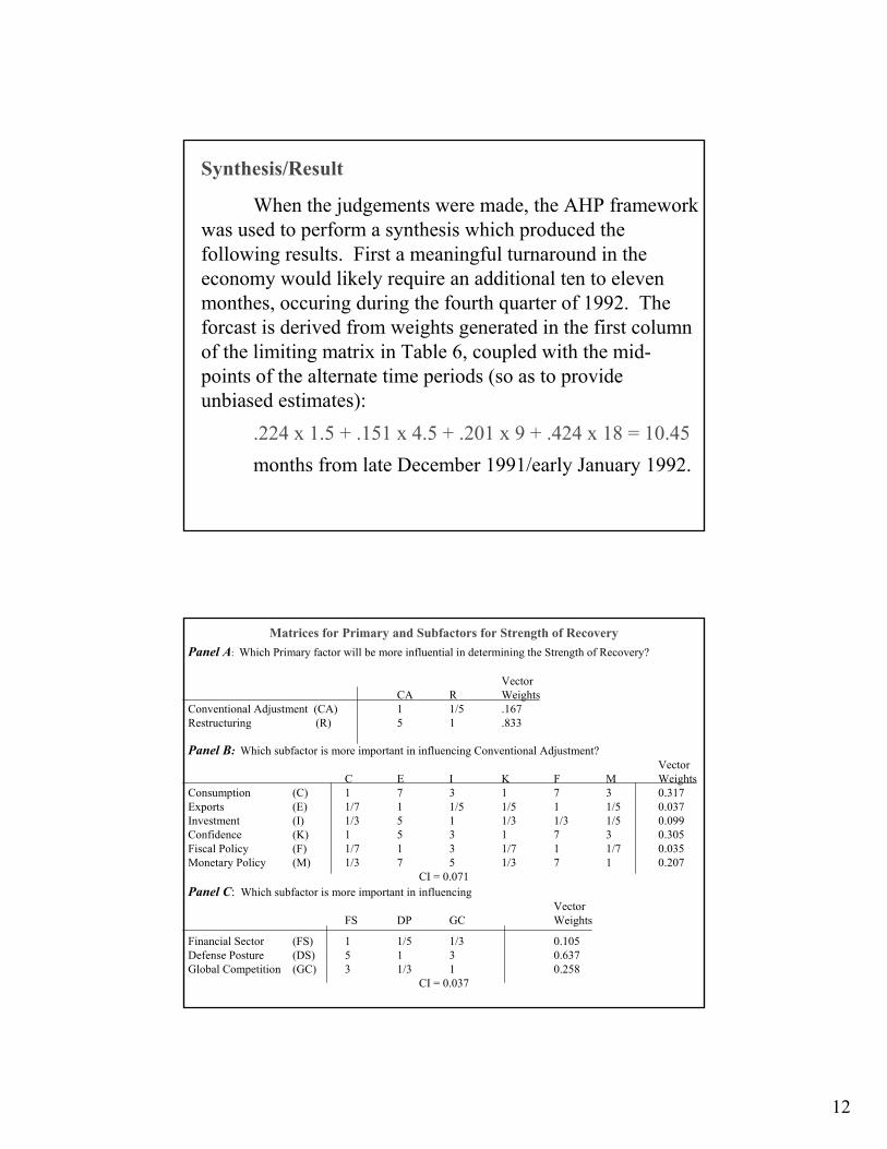
Synthesis/Result
When the judgements were made, the AHP framework was used to perform a synthesis which produced the following results. First a meaningful turnaround in the economy would likely require an additional ten to eleven monthes, occuring during the fourth quarter of 1992. The forcast is derived from weights generated in the first column of the limiting matrix in Table 6, coupled with the mid-points of the alternate time periods (so as to provide unbiased estimates):
.224 x 1.5 + .151 x 4.5 + .201 x 9 + .424 x 18 = 10.45months from late December 1991/early January 1992.
Matrices for Primary and Subfactors for Strength of RecoveryPanel A: Which Primary factor will be more influential in determining the Strength of Recovery?
VectorCA R Weights
Conventional Adjustment (CA) 1 1/5 .167Restructuring (R) 5 1 .833
Panel B: Which subfactor is more important in influencing Conventional Adjustment?Vector
C E I K F M WeightsConsumption (C) 1 7 3 1 7 3 0.317Exports (E) 1/7 1 1/5 1/5 1 1/5 0.037Investment (I) 1/3 5 1 1/3 1/3 1/5 0.099Confidence (K) 1 5 3 1 7 3 0.305Fiscal Policy (F) 1/7 1 3 1/7 1 1/7 0.035Monetary Policy (M) 1/3 7 5 1/3 7 1 0.207
CI = 0.071Panel C: Which subfactor is more important in influencing
VectorFS DP GC Weights
Financial Sector (FS) 1 1/5 1/3 0.105Defense Posture (DS) 5 1 3 0.637Global Competition (GC) 3 1/3 1 0.258
CI = 0.037
13
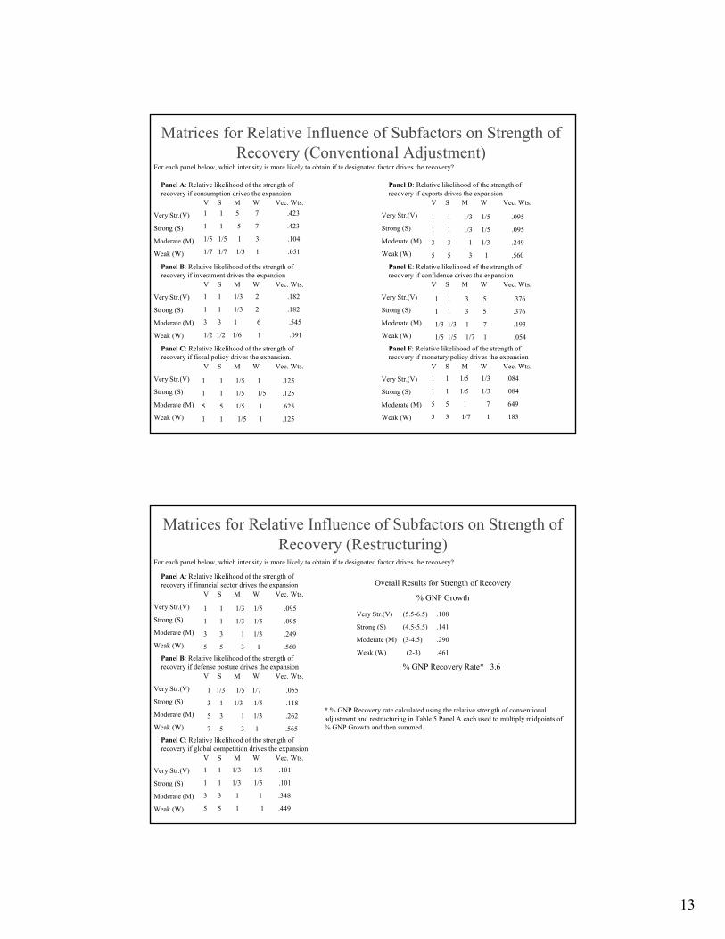
Matrices for Relative Influence of Subfactors on Strength of Recovery (Conventional Adjustment)
For each panel below, which intensity is more likely to obtain if te designated factor drives the recovery?
Panel A: Relative likelihood of the strength of recovery if consumption drives the expansion
V S M W Vec. Wts.
Very Str.(V)
Strong (S)
Moderate (M)
Weak (W)
Panel B: Relative likelihood of the strength of recovery if investment drives the expansion
V S M W Vec. Wts.
Very Str.(V)
Strong (S)
Moderate (M)
Weak (W)
Panel C: Relative likelihood of the strength of recovery if fiscal policy drives the expansion.
V S M W Vec. Wts.
Very Str.(V)
Strong (S)
Moderate (M)
Weak (W)
Panel D: Relative likelihood of the strength of recovery if exports drives the expansion
V S M W Vec. Wts.
Very Str.(V)
Strong (S)
Moderate (M)
Weak (W)
Panel E: Relative likelihood of the strength of recovery if confidence drives the expansion
V S M W Vec. Wts.
Very Str.(V)
Strong (S)
Moderate (M)
Weak (W)
Panel F: Relative likelihood of the strength of recovery if monetary policy drives the expansion
V S M W Vec. Wts.
Very Str.(V)
Strong (S)
Moderate (M)
Weak (W)
1 1 5 7 .423
1 1 5 7 .423
1/5 1/5 1 3 .104
1/7 1/7 1/3 1 .051
1 1 1/3 2 .182
1 1 1/3 2 .182
3 3 1 6 .545
1/2 1/2 1/6 1 .091
1 1 1/5 1 .125
1 1 1/5 1/5 .125
5 5 1/5 1 .625
1 1 1/5 1 .125
1 1 1/3 1/5 .095
1 1 1/3 1/5 .095
3 3 1 1/3 .249
5 5 3 1 .560
1 1 3 5 .376
1 1 3 5 .376
1/3 1/3 1 7 .193
1/5 1/5 1/7 1 .054
1 1 1/5 1/3 .084
1 1 1/5 1/3 .084
5 5 1 7 .649
3 3 1/7 1 .183
Matrices for Relative Influence of Subfactors on Strength of Recovery (Restructuring)
For each panel below, which intensity is more likely to obtain if te designated factor drives the recovery?
Panel A: Relative likelihood of the strength of recovery if financial sector drives the expansion
V S M W Vec. Wts.
Very Str.(V)
Strong (S)
Moderate (M)
Weak (W)
Panel B: Relative likelihood of the strength of recovery if defense posture drives the expansion
V S M W Vec. Wts.
Very Str.(V)
Strong (S)
Moderate (M)
Weak (W)
Panel C: Relative likelihood of the strength of recovery if global competition drives the expansion
V S M W Vec. Wts.
Very Str.(V)
Strong (S)
Moderate (M)
Weak (W)
1 1 1/3 1/5 .095
1 1 1/3 1/5 .095
3 3 1 1/3 .249
5 5 3 1 .560
1 1/3 1/5 1/7 .055
3 1 1/3 1/5 .118
5 3 1 1/3 .262
7 5 3 1 .565
1 1 1/3 1/5 .101
1 1 1/3 1/5 .101
3 3 1 1 .348
5 5 1 1 .449
Overall Results for Strength of Recovery
% GNP Growth
Very Str.(V)
Strong (S)
Moderate (M)
Weak (W)
(5.5-6.5) .108
(4.5-5.5) .141
(3-4.5) .290
(2-3) .461
% GNP Recovery Rate* 3.6
* % GNP Recovery rate calculated using the relative strength of conventional adjustment and restructuring in Table 5 Panel A each used to multiply midpoints of % GNP Growth and then summed.
14
Tighter.191
Steady.082
Easier.191
FederalReserve Mon.
Policy.294
Contract.002No
Change.009
Expand.021
Size ofFederalDeficit
.032
Tighter.007
Steady.027
Easier.063
Bank ofJapan Monet.
Policy.097
RelativeInterest
Rate.423
High.002Medium
.002Low.002
Forward RatePremium/Discount
.007
Premium.008
Discount.008
Size ofForward rateDifferential
.016
ForwardExchangeRate Bias
.023
Strong.026
Moderate.100
Weak.011
Con-sistent
.137
Strong.009
Moderate.009
Weak.009
erratic.027
OfficialExchg. Mkt.Intervention
.164
Higher.013
Equal.006
Lower.001
RelativeInfaltion
Rates.019
Higher.003
Equal.003
Lower.003
RelativeReal
Growth.008
More.048Equal.022
Less.006
RelativePoliticalStability
.075
Rel. Deg. ofConfid. in
the US Econ..103
Large.016
Small.016
Size ofDeficit orSurplus
.032
Decrease.090
No Charge.106
Increase.025
Antici-pated
Changes.221
Size/Direction ofUS Current Acct.
Balance.252
High.001Medium
.001Low.001
Rele-vant.004
High.010Med..010Low.010
Irrele-vant.031
Past Behavior ofExchange Rates
.035
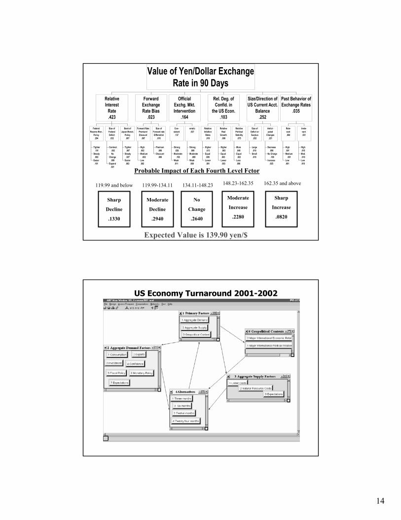
Value of Yen/Dollar ExchangeRate in 90 Days
Probable Impact of Each Fourth Level Fctor
Sharp
Decline
.1330
Moderate
Decline
.2940
No
Change
.2640
Moderate
Increase
.2280
Sharp
Increase
.0820
119.99 and below 119.99-134.11 134.11-148.23 148.23-162.35 162.35 and above
Expected Value is 139.90 yen/$
US Economy Turnaround 2001-2002
15
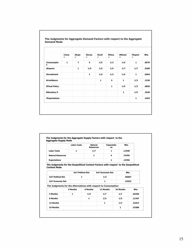
1Cons~
2Expo~
3Inves~
4Conf~
5Fisca~
6Monet~
7Expect~
Wts.
1Consumption
1 7 5 1/5 1/2 1/5 1 .0979
2Exports 1 1/5 1/5 1/5 1/7 1/7 .0209
3Investment 1 1/5 1/3 1/5 1 .0564
4Confidence 1 5 1 1/3 .2220
5Fiscal Policy 1 1/5 1/3 .0835
6Monetary P. 1 1/5 .3540
7Expectations 1 .1653
The Judgments for Aggregate Demand Factors with respect to the Aggregate Demand Node
Labor Costs Natural Resources
Expectations
Wts.
Labor Costs 1 1/7 1 .11940
Natural Resources 1 5 .74705
Expectations 1 .13356
The Judgments for the Aggregate Supply Factors with respect to the Aggregate Supply Node
The Judgments for the Geopolitical Context Factors with respect to the Geopolitical Context Node
Int’l Political Rel. Int’l Economic Rel. Wts.
Int’l Political Rel. 1 1/2 .66667
Int’l Economic Rel. 1 .33333
The Judgments for the Alternatives with respect to Consumption3 Months 6 Months 12 Months 24 Months Wts.
3 Months 1 1/5 1/7 1/7 .04259
6 Months 1 1/5 1/5 .11347
12 Months 1 1/3 .31014
24 Months 1 .53380
16
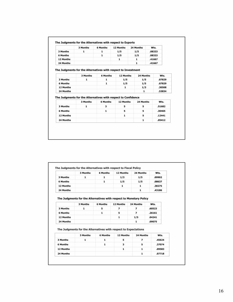
The Judgments for the Alternatives with respect to Exports
3 Months 6 Months 12 Months 24 Months Wts.
3 Months 1 1 1/5 1/5 .08333
6 Months 1 1/5 1/5 .08333
12 Months 1 1 .41667
24 Months 1 .41667
The Judgments for the Alternatives with respect to Investment
3 Months 6 Months 12 Months 24 Months Wts.
3 Months 1 1 1/5 1/5 .07829
6 Months 1 1/5 1/5 .07829
12 Months 1 1/3 .30508
24 Months 1 .53834
The Judgments for the Alternatives with respect to Confidence3 Months 6 Months 12 Months 24 Months Wts.
3 Months 1 3 5 5 .51682
6 Months 1 5 5 .30465
12 Months 1 5 .12441
24 Months 1 .05412
The Judgments for the Alternatives with respect to Fiscal Policy
3 Months 6 Months 12 Months 24 Months Wts.
3 Months 1 1 1/3 1/5 .09902
6 Months 1 1/5 1/5 .08637
12 Months 1 1 .38275
24 Months 1 .43186
The Judgments for the Alternatives with respect to Monetary Policy
3 Months 6 Months 12 Months 24 Months Wts.
3 Months 1 5 7 7 .60523
6 Months 1 5 7 .26161
12 Months 1 1/5 .04241
24 Months 1 .09075
The Judgments for the Alternatives with respect to Expectations
3 Months 6 Months 12 Months 24 Months Wts.
3 Months 1 1 5 7 .45624
6 Months 1 3 5 .37074
12 Months 1 1 .09583
24 Months 1 .07718
17
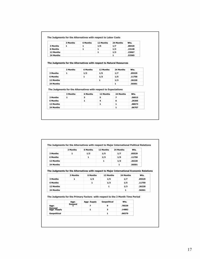
The Judgments for the Alternatives with respect to Labor Costs
3 Months 6 Months 12 Months 24 Months Wts.
3 Months 1 1 1/5 1/7 .08420
6 Months 1 1 1/3 .1514812 Months 1 1/3 .2306724 Months 1 .53365
The Judgments for the Alternatives with respect to Natural Resources
3 Months 6 Months 12 Months 24 Months Wts.
3 Months 1 1/3 1/5 1/7 .05529
6 Months 1 1/3 1/5 .11750
12 Months 1 1/3 .26220
24 Months 1 .56501
The Judgments for the Alternatives with respect to Expectations
3 Months 6 Months 12 Months 24 Months Wts.
3 Months 1 3 5 7 .56015
6 Months 1 4 6 .29205
12 Months 1 1 .08073
24 Months 1 .06707
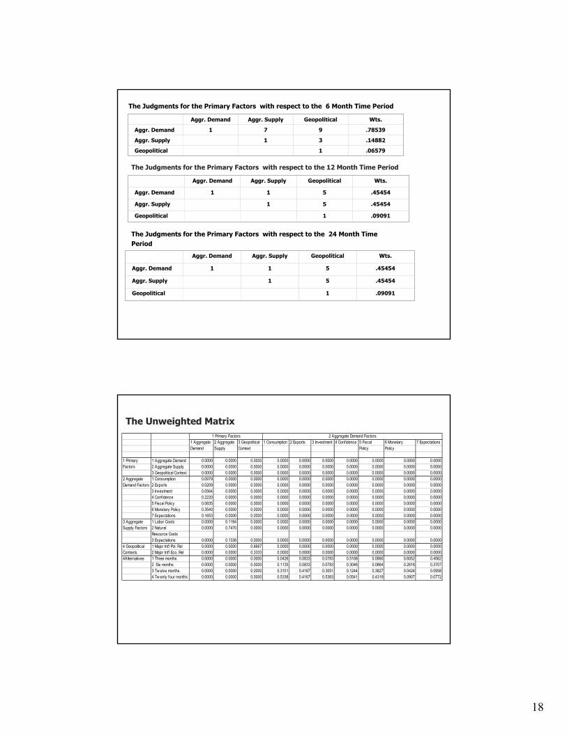
The Judgments for the Alternatives with respect to Major International Political Relations
3 Months 6 Months 12 Months 24 Months Wts.
3 Months 1 1/3 1/5 1/7 .05529
6 Months 1 1/3 1/5 .11750
12 Months 1 1/3 .26220
24 Months 1 .56501
The Judgments for the Alternatives with respect to Major International Economic Relations
3 Months 6 Months 12 Months 24 Months Wts.
3 Months 1 1/3 1/5 1/7 .05529
6 Months 1 1/3 1/5 .11750
12 Months 1 1/3 .26220
24 Months 1 .56501
The Judgments for the Primary Factors with respect to the 3 Month Time Period
Aggr. Demand
Aggr. Supply Geopolitical Wts.
Aggr. Demand
1 7 9 .78539
Aggr. Supply 1 3 .14882
Geopolitical 1 .06579
18
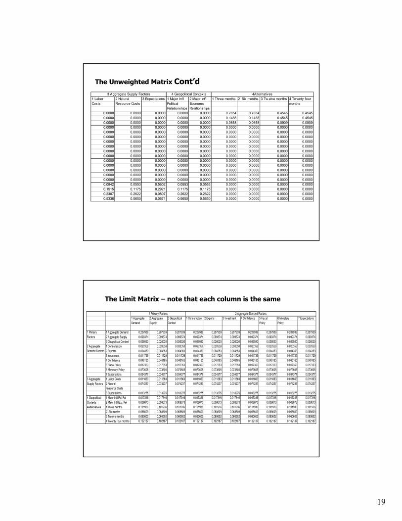
The Judgments for the Primary Factors with respect to the 6 Month Time Period
Aggr. Demand Aggr. Supply Geopolitical Wts.
Aggr. Demand 1 7 9 .78539
Aggr. Supply 1 3 .14882
Geopolitical 1 .06579
The Judgments for the Primary Factors with respect to the 12 Month Time Period
Aggr. Demand Aggr. Supply Geopolitical Wts.
Aggr. Demand 1 1 5 .45454
Aggr. Supply 1 5 .45454
Geopolitical 1 .09091
The Judgments for the Primary Factors with respect to the 24 Month Time Period
Aggr. Demand Aggr. Supply Geopolitical Wts.
Aggr. Demand 1 1 5 .45454
Aggr. Supply 1 5 .45454
Geopolitical 1 .09091
The Unweighted Matrix
1 Aggregate 2 Aggregate 3 Geopolitical 1 Consumption 2 Exports 3 Investment 4 Confidence 5 Fiscal 6 Monetary 7 ExpectationsDemand Supply Context Policy Policy
1 Primary 1 Aggregate Demand 0.0000 0.0000 0.0000 0.0000 0.0000 0.0000 0.0000 0.0000 0.0000 0.0000Factors 2 Aggregate Supply 0.0000 0.0000 0.0000 0.0000 0.0000 0.0000 0.0000 0.0000 0.0000 0.0000
3 Geopolitical Context 0.0000 0.0000 0.0000 0.0000 0.0000 0.0000 0.0000 0.0000 0.0000 0.00002 Aggregate 1 Consumption 0.0979 0.0000 0.0000 0.0000 0.0000 0.0000 0.0000 0.0000 0.0000 0.0000Demand Factors 2 Exports 0.0209 0.0000 0.0000 0.0000 0.0000 0.0000 0.0000 0.0000 0.0000 0.0000
3 Investment 0.0564 0.0000 0.0000 0.0000 0.0000 0.0000 0.0000 0.0000 0.0000 0.00004 Confidence 0.2220 0.0000 0.0000 0.0000 0.0000 0.0000 0.0000 0.0000 0.0000 0.00005 Fiscal Policy 0.0835 0.0000 0.0000 0.0000 0.0000 0.0000 0.0000 0.0000 0.0000 0.00006 Monetary Policy 0.3540 0.0000 0.0000 0.0000 0.0000 0.0000 0.0000 0.0000 0.0000 0.00007 Expectations 0.1653 0.0000 0.0000 0.0000 0.0000 0.0000 0.0000 0.0000 0.0000 0.0000
3 Aggregate 1 Labor Costs 0.0000 0.1194 0.0000 0.0000 0.0000 0.0000 0.0000 0.0000 0.0000 0.0000Supply Factors 2 Natural 0.0000 0.7470 0.0000 0.0000 0.0000 0.0000 0.0000 0.0000 0.0000 0.0000
Resource Costs3 Expectations 0.0000 0.1336 0.0000 0.0000 0.0000 0.0000 0.0000 0.0000 0.0000 0.0000
4 Geopolitical 1 Major Int'l Pol. Rel 0.0000 0.0000 0.6667 0.0000 0.0000 0.0000 0.0000 0.0000 0.0000 0.0000Contexts 2 Major Int'l Eco. Rel 0.0000 0.0000 0.3333 0.0000 0.0000 0.0000 0.0000 0.0000 0.0000 0.00004Alternatives 1 Three months 0.0000 0.0000 0.0000 0.0426 0.0833 0.0783 0.5168 0.0990 0.6052 0.4562
2 Six months 0.0000 0.0000 0.0000 0.1135 0.0833 0.0783 0.3046 0.0864 0.2616 0.37073 Tw elve months 0.0000 0.0000 0.0000 0.3101 0.4167 0.3051 0.1244 0.3827 0.0424 0.09584 Tw enty four months 0.0000 0.0000 0.0000 0.5338 0.4167 0.5383 0.0541 0.4319 0.0907 0.0772
2 Aggregate Demand Factors1 Primary Factors
19
The Unweighted Matrix Cont’d
1 Labor 2 Natural 3 Expectations 1 Major Int'l 2 Major Int'l 1 Three months 2 Six months 3 Tw elve months 4 Tw enty four Costs Resource Costs Political Economic months
Relationships Relationships0.0000 0.0000 0.0000 0.0000 0.0000 0.7854 0.7854 0.4545 0.45450.0000 0.0000 0.0000 0.0000 0.0000 0.1488 0.1488 0.4545 0.45450.0000 0.0000 0.0000 0.0000 0.0000 0.0658 0.0658 0.0909 0.09090.0000 0.0000 0.0000 0.0000 0.0000 0.0000 0.0000 0.0000 0.00000.0000 0.0000 0.0000 0.0000 0.0000 0.0000 0.0000 0.0000 0.00000.0000 0.0000 0.0000 0.0000 0.0000 0.0000 0.0000 0.0000 0.00000.0000 0.0000 0.0000 0.0000 0.0000 0.0000 0.0000 0.0000 0.00000.0000 0.0000 0.0000 0.0000 0.0000 0.0000 0.0000 0.0000 0.00000.0000 0.0000 0.0000 0.0000 0.0000 0.0000 0.0000 0.0000 0.00000.0000 0.0000 0.0000 0.0000 0.0000 0.0000 0.0000 0.0000 0.00000.0000 0.0000 0.0000 0.0000 0.0000 0.0000 0.0000 0.0000 0.00000.0000 0.0000 0.0000 0.0000 0.0000 0.0000 0.0000 0.0000 0.00000.0000 0.0000 0.0000 0.0000 0.0000 0.0000 0.0000 0.0000 0.00000.0000 0.0000 0.0000 0.0000 0.0000 0.0000 0.0000 0.0000 0.00000.0000 0.0000 0.0000 0.0000 0.0000 0.0000 0.0000 0.0000 0.00000.0842 0.0553 0.5602 0.0553 0.0553 0.0000 0.0000 0.0000 0.00000.1515 0.1175 0.2921 0.1175 0.1175 0.0000 0.0000 0.0000 0.00000.2307 0.2622 0.0807 0.2622 0.2622 0.0000 0.0000 0.0000 0.00000.5336 0.5650 0.0671 0.5650 0.5650 0.0000 0.0000 0.0000 0.0000
4Alternatives3 Aggregate Supply Factors 4 Geopolitical Contexts
The Limit Matrix – note that each column is the same
1 Aggregate 2 Aggregate 3 Geopolitical 1 Consumption 2 Exports 3 Investment 4 Conf idence 5 Fiscal 6 Monetary 7 ExpectationsDemand Supply Context Policy Policy
1 Primary 1 Aggregate Demand 0.207939 0.207939 0.207939 0.207939 0.207939 0.207939 0.207939 0.207939 0.207939 0.207939Factors 2 Aggregate Supply 0.099374 0.099374 0.099374 0.099374 0.099374 0.099374 0.099374 0.099374 0.099374 0.099374
3 Geopolitical Context 0.026020 0.026020 0.026020 0.026020 0.026020 0.026020 0.026020 0.026020 0.026020 0.0260202 Aggregate 1 Consumption 0.020358 0.020358 0.020358 0.020358 0.020358 0.020358 0.020358 0.020358 0.020358 0.020358Demand Factors 2 Exports 0.004353 0.004353 0.004353 0.004353 0.004353 0.004353 0.004353 0.004353 0.004353 0.004353
3 Investment 0.011729 0.011729 0.011729 0.011729 0.011729 0.011729 0.011729 0.011729 0.011729 0.0117294 Conf idence 0.046165 0.046165 0.046165 0.046165 0.046165 0.046165 0.046165 0.046165 0.046165 0.0461655 Fiscal Policy 0.017353 0.017353 0.017353 0.017353 0.017353 0.017353 0.017353 0.017353 0.017353 0.0173536 Monetary Policy 0.073605 0.073605 0.073605 0.073605 0.073605 0.073605 0.073605 0.073605 0.073605 0.0736057 Expectations 0.034377 0.034377 0.034377 0.034377 0.034377 0.034377 0.034377 0.034377 0.034377 0.034377
3 Aggregate 1 Labor Costs 0.011863 0.011863 0.011863 0.011863 0.011863 0.011863 0.011863 0.011863 0.011863 0.011863Supply Factors 2 Natural 0.074237 0.074237 0.074237 0.074237 0.074237 0.074237 0.074237 0.074237 0.074237 0.074237
Resource Costs3 Expectations 0.013275 0.013275 0.013275 0.013275 0.013275 0.013275 0.013275 0.013275 0.013275 0.013275
4 Geopolitical 1 Major Int'l Pol. Rel 0.017346 0.017346 0.017346 0.017346 0.017346 0.017346 0.017346 0.017346 0.017346 0.017346Contexts 2 Major Int'l Eco. Rel 0.008673 0.008673 0.008673 0.008673 0.008673 0.008673 0.008673 0.008673 0.008673 0.0086734Alternatives 1 Three months 0.101936 0.101936 0.101936 0.101936 0.101936 0.101936 0.101936 0.101936 0.101936 0.101936
2 Six months 0.068609 0.068609 0.068609 0.068609 0.068609 0.068609 0.068609 0.068609 0.068609 0.0686093 Tw elve months 0.060602 0.060602 0.060602 0.060602 0.060602 0.060602 0.060602 0.060602 0.060602 0.0606024 Tw enty four months 0.102187 0.102187 0.102187 0.102187 0.102187 0.102187 0.102187 0.102187 0.102187 0.102187
1 Primary Factors 2 Aggregate Demand Factors
20
1 Labor 2 Natural 3 Expectations 1 Major Int'l 2 Major Int'l 1 Three months 2 Six months 3 Tw elve months 4 Tw enty four Costs Resource Costs Political Economic months
Relationships Relationships0.207939 0.207939 0.207939 0.207939 0.207939 0.207939 0.207939 0.207939 0.2079390.099374 0.099374 0.099374 0.099374 0.099374 0.099374 0.099374 0.099374 0.0993740.026020 0.026020 0.026020 0.026020 0.026020 0.026020 0.026020 0.026020 0.0260200.020358 0.020358 0.020358 0.020358 0.020358 0.020358 0.020358 0.020358 0.0203580.004353 0.004353 0.004353 0.004353 0.004353 0.004353 0.004353 0.004353 0.0043530.011729 0.011729 0.011729 0.011729 0.011729 0.011729 0.011729 0.011729 0.0117290.046165 0.046165 0.046165 0.046165 0.046165 0.046165 0.046165 0.046165 0.0461650.017353 0.017353 0.017353 0.017353 0.017353 0.017353 0.017353 0.017353 0.0173530.073605 0.073605 0.073605 0.073605 0.073605 0.073605 0.073605 0.073605 0.0736050.034377 0.034377 0.034377 0.034377 0.034377 0.034377 0.034377 0.034377 0.0343770.011863 0.011863 0.011863 0.011863 0.011863 0.011863 0.011863 0.011863 0.0118630.074237 0.074237 0.074237 0.074237 0.074237 0.074237 0.074237 0.074237 0.074237
0.013275 0.013275 0.013275 0.013275 0.013275 0.013275 0.013275 0.013275 0.0132750.017346 0.017346 0.017346 0.017346 0.017346 0.017346 0.017346 0.017346 0.0173460.008673 0.008673 0.008673 0.008673 0.008673 0.008673 0.008673 0.008673 0.0086730.101936 0.101936 0.101936 0.101936 0.101936 0.101936 0.101936 0.101936 0.1019360.068609 0.068609 0.068609 0.068609 0.068609 0.068609 0.068609 0.068609 0.0686090.060602 0.060602 0.060602 0.060602 0.060602 0.060602 0.060602 0.060602 0.0606020.102187 0.102187 0.102187 0.102187 0.102187 0.102187 0.102187 0.102187 0.102187
4Alternatives3 Aggregate Supply Factors 4 Geopolitical Contexts
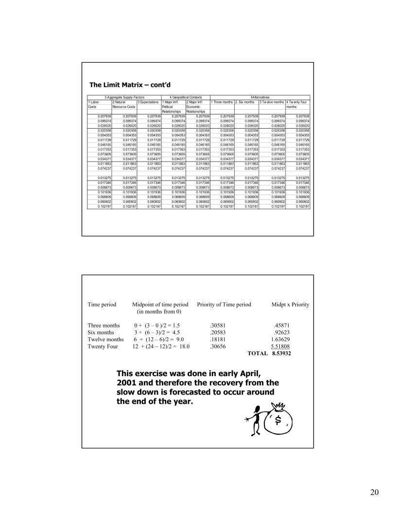
The Limit Matrix – cont’d
Time period Midpoint of time period Priority of Time period Midpt x Priority(in months from 0)
Three months 0 + (3 – 0 )/2 = 1.5 .30581 .45871Six months 3 + (6 – 3)/2 = 4.5 .20583 .92623Twelve months 6 + (12 – 6)/2 = 9.0 .18181 1.63629Twenty Four 12 + (24 – 12)/2 = 18.0 .30656 5.51808
TOTAL 8.53932
This exercise was done in early April, 2001 and therefore the recovery from the slow down is forecasted to occur around the end of the year.
21
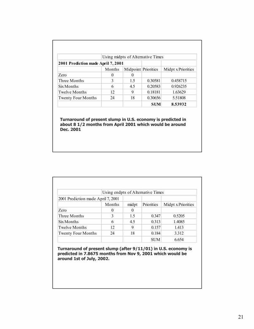
Turnaround of present slump in U.S. economy is predicted in about 8 1/2 months from April 2001 which would be around Dec. 2001
Using midpts of Alternative Times2001 Prediction made April 7, 2001
Months Midpoint Priorities Midpt x PrioritiesZero 0 0Three Months 3 1.5 0.30581 0.458715Six Months 6 4.5 0.20583 0.926235Twelve Months 12 9 0.18181 1.63629Twenty Four Months 24 18 0.30656 5.51808
SUM 8.53932
Turnaround of present slump (after 9/11/01) in U.S. economy is predicted in 7.8675 months from Nov 9, 2001 which would be around 1st of July, 2002.
Using endpts of Alternative Times2001 Prediction made April 7, 2001
Months midpt Priorities Midpt x PrioritiesZero 0 0Three Months 3 1.5 0.347 0.5205Six Months 6 4.5 0.313 1.4085Twelve Months 12 9 0.157 1.413Twenty Four Months 24 18 0.184 3.312
SUM 6.654