Combustion and Flame 157 (2010) 1850–1862

Contents lists available at ScienceDirect

Combustion and Flame

journal homepage: www.elsevier .com/locate /combustflame

Prediction of autoignition in a lifted methane/air flame using an unsteadyflamelet/progress variable model

Matthias Ihme *, Yee Chee SeeDepartment of Aerospace Engineering, University of Michigan, Ann Arbor, MI 48109, United States

a r t i c l e i n f o a b s t r a c t

Article history:Received 19 July 2009Received in revised form 27 September 2009Accepted 15 July 2010Available online 3 August 2010

Keywords:Turbulent combustionAutoignitionLifted flamesNon-premixed combustionUnsteady flamelet modelingLarge-eddy simulation

0010-2180/$ - see front matter � 2010 The Combustdoi:10.1016/j.combustflame.2010.07.015

* Corresponding author. Fax: +1 734 763 0578.E-mail address: mihme@umich.edu (M. Ihme).

An unsteady flamelet/progress variable (UFPV) model has been developed for the prediction of autoigni-tion in turbulent lifted flames. The model is a consistent extension to the steady flamelet/progress vari-able (SFPV) approach, and employs an unsteady flamelet formulation to describe the transient evolutionof all thermochemical quantities during the flame ignition process. In this UFPV model, all thermochem-ical quantities are parameterized by mixture fraction, reaction progress parameter, and stoichiometricscalar dissipation rate, eliminating the explicit dependence on a flamelet time scale. An a priori studyis performed to analyze critical modeling assumptions that are associated with the population of theflamelet state space.

For application to LES, the UFPV model is combined with a presumed PDF closure to account for subgridcontributions of mixture fraction and reaction progress variable. The model was applied in LES of a liftedmethane/air flame. Additional calculations were performed to quantify the interaction between turbu-lence and chemistry a posteriori. Simulation results obtained from these calculations are compared withexperimental data. Compared to the SFPV results, the unsteady flamelet/progress variable model capturesthe autoignition process, and good agreement with measurements is obtained for mixture fraction, tem-perature, and species mass fractions. From the analysis of scatter data and mixture fraction-conditionalresults it is shown that the turbulence/chemistry interaction delays the ignition process towards lowervalues of scalar dissipation rate, and a significantly larger region in the flamelet state space is occupiedduring the ignition process.

� 2010 The Combustion Institute. Published by Elsevier Inc. All rights reserved.

1. Introduction

The development of advanced combustion systems is mainlycontrolled by the objective to increase fuel efficiency and to reduceemissions of pollutants such as carbon monoxide (CO), unburnedhydrocarbons (UHC), and nitrogen oxides (NOx). To address theseissues, combustion strategies have been developed that utilizecombustion of lean and diluted fuel–air mixtures. In these systems,dilution is frequently accomplished through the recirculation ofburned gases, which reduces the combustion temperature, andinhibits the formation of thermal nitric oxide. In addition to re-duced pollutant emissions, the dilution with hot combustion prod-ucts can also lead to improved flame stability [1].

Despite its enormous potential, the stable combustion of leanand diluted fuel–air mixtures introduces considerable challenges.In particular, the dilution of reactants with inert combustion prod-ucts can lead to a reduction in the characteristic Damköhler num-ber, so that – unlike conventional diffusion flames, in which thecombustion process is primarily mixing-controlled – the reaction

ion Institute. Published by Elsevier

kinetics becomes increasingly important. As such, the stabilityand characteristics of the flame becomes particularly sensitive tovariations in fuel composition and operating conditions. Therefore,ignition mechanisms in such flames play a critical role and are di-rectly affected by the turbulence/chemistry interaction.

Recently, Yoo et al. [2] performed direct numerical simulations(DNS) to investigate autoignition of a lifted hydrogen flame in a co-flow at elevated temperature. Their results showed that the flamestabilizes in regions where the reactants are incompletely mixedand autoignition occurs under conditions in which gradients of fueland oxidizer are oriented in opposite directions. The autoignitionprocess could be associated with the accumulation of hydroperoxyl(HO2) upstream of the flamebase, providing a source of hydroxyl(OH) radicals for the autoignition. With increasing downstreamdistance, the heat release extends towards the fuel-rich composi-tion and occurs under premixed and non-premixed conditions.

Autoignition of a fuel mixture in a hot environment is typicallyinitiated in localized regions of low scalar dissipation rates havinga mixture composition that favors short ignition times. Since theprediction of autoignition events is strongly dependent on thestructure of the surrounding turbulent reacting flow environment,combustion models are required that are able to provide an

Inc. All rights reserved.

M. Ihme, Y.C. See / Combustion and Flame 157 (2010) 1850–1862 1851

accurate characterization of the spatiotemporal flow field struc-ture. Although large-eddy simulation (LES) techniques have beendemonstrated to provide improved predictions for the turbulentmixing process compared to Reynolds-averaged Navier–Stokes(RANS) approaches [3], these intermittent ignition events typicallyoccur on scales that are computationally not resolved. Therefore,subgrid-scale closure models are required to characterize effectsof unresolved scales and ignition kinetics. By addressing these is-sues, the objective of this work is to develop a LES combustionmodel for application to autoignition in turbulent non-premixedflames. To this end, an unsteady flamelet formulation that wasdeveloped by Pitsch and Ihme [4] is extended. In this model, thetransient flame evolution is characterized by mixture fraction,reaction progress variable, and scalar dissipation rate, and theflame structure is obtained from the unsteady flamelet equations.A potential advantage over related formulations [5] is that thismodel eliminates the explicit dependence on the time-scale infor-mation which leads to significant simplifications in the computa-tion and parameterization of the thermodynamic state space.

The LES autoignition model is applied to a lifted methane/air jetflame. This flame configuration was experimentally investigated byCabra et al. [6], and consists of a central fuel jet which issues amethane/air mixture into a vitiated co-flow. The temperature ofthe co-flow stream is 1355 K. Following a region in which fueland oxidizer mix without significant heat release, the flame ignitesand stabilizes at a lift-off height of approximately 30 nozzle diam-eters downstream of the jet exit.

Because of its canonical geometry, comprehensive experimentaldatabase, and sensitivity of the flame characteristics to operatingconditions, this flame configuration has gained particular interestin the computational combustion community, and is frequentlyused for validation and development of combustion models. Gordonet al. [7] investigated the transport budget of this flame using a com-position PDF approach. From this study they concluded that theflame stabilization mechanism is primarily controlled by autoigni-tion. A joint scalar transported PDF approach with detailed reactionchemistry coupled with a second moment closure model for thevelocity prediction was used by Gkagkas and Lindstedt [8] to com-pute this lifted flame. Their model reproduced the flow field sensitiv-ity to boundary conditions, and the role of hydroperoxyl andformaldehyde on the ignition kinetics was characterized. Domingoet al. [9] performed a LES calculation of this flame. They combineda model for autoignition in a perfectly stirred reactor (PSR) with amodel for partially premixed flame propagation, and good agree-ment between simulation results and experimental data was ob-tained. More recently, Michel et al. [10] conducted a RANSsimulation of this flame using an approximate diffusion flame ap-proach. In this approach, the transient flame states are obtained froma PSR calculation, and diffusive effects are considered a posteriorithrough the solution of a diffusion flamelet equation for a progressvariable.

In this context it is interesting to point out that all of these calcu-lations employed combustion models that either rely on a trans-ported PDF approach or a formulation in which a PSR model isemployed to model the autoignition process. However, non-pre-mixed combustion models have so far not been applied to this flame.This paper addresses this shortcoming, and specifically focuses ontwo aspects, namely the characterization of transient effects in thecontext of diffusion flames, and the role of the turbulence/chemistryinteraction that is of particular relevance to LES applications.

The remainder of this paper is organized as follows. The math-ematical model describing the unsteady flamelet/progress variableformulation and the presumed PDF closure is presented in the nextsection. The experimental configuration and computational setupare summarized in Section 3. An a priori study is performed in Sec-tion 4 to analyze critical modeling assumptions that are associated

with the population of the flamelet state space. Following this apriori study, the model is applied in LES, and simulation resultsare discussed in Section 5. The paper finishes with conclusions.

2. Mathematical model

2.1. Large-eddy simulation

In LES, coherent large scale structures of the turbulent flow arecomputationally resolved, and effects of smaller and numericallyunresolved scales on the large scales are modeled. The decomposi-tion of the scales is achieved by applying a low-pass filter to theflow field quantities. In the case of a reacting flow, the Favre-fil-tered quantity of a scalar w is computed as

ewðt; xÞ ¼ 1q

Zqðt; yÞwðt; yÞGðt; x; y; DÞdy; ð1Þ

where t denotes time, x is the spatial coordinate, q is the density,and G is the filter kernel. The residual field is defined asw00ðt; xÞ ¼ wðt; xÞ � ewðt; xÞ and Favre-filtered quantities are relatedto Reynolds-filtered quantities by qew ¼ qw:

After applying the filter operator to the instantaneous govern-ing equations, describing the conservation of mass and momen-tum, the Favre-filtered equations can be written aseDtq ¼ �qr � eu; ð2aÞq eDteu ¼ �rpþr � rþr � rres; ð2bÞ

where q is the filtered density, eu is the filtered velocity vector, p isthe filtered pressure, eDt ¼ @t þ eu � r is the Favre-filtered substan-tial derivative, and r is the filtered viscous stress tensor with

r ¼ 2qem eS � 13ðr � euÞI� �

and eS ¼ 12½reu þ ðreuÞT �: ð3Þ

The residual stress tensor, rres ¼ qeueu � qfuu, appears in unclosedform, and is modeled by a dynamic Smagorinsky model [11,12].In deriving Eq. (2) a time-invariant filter is used, and commutationerrors due to grid size variations are neglected [13]. The density andmolecular properties, appearing in Eqs. (2) and (3), and all otherthermochemical quantities are obtained from the flamelet/progressvariable model. This model and its extension to autoignition predic-tion are discussed in the next sections.

2.2. Flamelet/progress variable model

The flamelet/progress variable (FPV) model [14,15] is based onthe flamelet equations, in which a turbulent diffusion flame is rep-resented as an ensemble of laminar flame structures [16,17]. Forsufficiently large Damköhler number or activation energy, chemi-cal reactions and heat transfer occur in a thin layer. If the charac-teristic length scale of this layer is small compared to that of thesurrounding turbulence, turbulent structures are unable to pene-trate into the reaction zone and cannot destroy the flame structure.Therefore, effects of turbulence only result in a deformation andstraining of the flame sheet.

The flamelet equations are obtained through a coordinate trans-formation of the transport equations for species mass fraction andtemperature [16,17], in which the mixture fraction Z is introducedas an independent variable. The unsteady flamelet equations canthen be written as

@t/�vZ

2@2

Z/ ¼ _x; ð4Þ

where _x corresponds to the source term of all species and temper-ature, which are collectively denoted by the vector /. The scalar dis-sipation rate of the mixture fraction, appearing in Eq. (4), is

0.1 1 10 100 10001000

1500

2000

2500

0.05 0.1 0.15 0.2 0.25 0.31000

1500

2000

2500

0.05

0.1

0.15

0.2

0.25

0.3

Fig. 1. Mapping between C and K: The top panel shows the temperature andreaction progress variable as a function of vZ,st along the entire S-shaped curve. Byremapping the same data onto the reaction progress parameter K (shown in thebottom panel) a unique representation of the entire S-shaped curve is obtained. Forreference, an unsteady flamelet trajectory for a constant scalar dissipation rate ofvZ,st = 100 s�1 is shown by the symbols.

1852 M. Ihme, Y.C. See / Combustion and Flame 157 (2010) 1850–1862

vZ ¼ 2ajrZj2; ð5Þ

and a is the mass diffusivity, which is assumed to be equal for allspecies. An analytical expression for vZ for a counter-flow diffusionflame was derived by Peters [18]. This expression relates vZ to itsvalue at stoichiometric condition and is a function of Z and Zst:

vZ ¼ vZ;stFðZÞ

with

FðZÞ ¼ exp 2 erfc�1ð2ZstÞh i2

� ½ erfc�1ð2ZÞ�2� �� �

; ð6Þ

and erfc�1 denotes the inverse of the complementary error function.

2.3. Steady flamelet/progress variable (SFPV) model

The steady flamelet equations can be derived from Eq. (4) underthe consideration that all species are formed on a sufficiently fasttime scale, so that all species mass fractions and temperature arein quasi steady state. With this, temporal derivatives become neg-ligible, and Eq. (4) reduces to

�vZ

2@2

Z/ ¼ _x: ð7Þ

The solution of these equations can be represented by the so-calledS-shaped curve [18], and all thermochemical quantities can then beparameterized in terms of mixture fraction and scalar dissipationrate, viz.,

w ¼ EwðZ;vZ;stÞ; ð8Þ

in which Ew corresponds to the steady-state flamelet relation, and wdenotes all thermochemical quantities, including molecular proper-ties, density, temperature, species mass fractions, and chemicalsource terms. The Favre-filtered form of this state relation can beused to provide information about density and molecular propertiesthat are necessary to solve Eq. (2). In addition to the governingequations describing conservation of mass and momentum, anadditional transport equation for the mixture fraction must besolved, and the scalar dissipation rate can be obtained from an alge-braic relation. Note however, that this representation is not uniqueand results in multiple solutions for certain values of scalar dissipa-tion rates.

To overcome the ambiguity of the steady flamelet model, a reac-tion progress parameter K has been introduced in the SFPV model[15]. This mixture fraction-independent parameter, which is relatedto the reaction progress variable C, is defined so that each flameletalong the entire S-shaped curve can be uniquely identified. In thefollowing, the reaction progress variable is defined from a linearcombination of reaction products as C ¼ YCO þ YCO2 þ YH2O þ YH2 . Iffor each flamelet K is associated with the corresponding C at stoi-chiometric condition, a unique mapping between vZ,st and K alongthe entire S-shaped curve is obtained. Figure 1 illustrates thismapping procedure. The top panel shows the temperature and thereaction progress variable as a function of vZ,st. The bottom panelshows the corresponding data for Tst, obtained by remapping thesolution from vZ,st onto the reaction progress parameter K. The re-sults illustrated in this figure emphasize the unique representationof each flamelet along the entire S-shaped curve. By remappingEq. (8), the SFPV state relation can be written as

w ¼FSwðZ;KÞ; ð9Þ

where the superscript ‘‘S” refers to the steady flamelet equations inthe SFPV model. This relation is used instead of Eq. (8) to representthe complete thermochemical state space along the entire S-shapedcurve.

Although this SFPV model has been successfully applied to awide range of combustion configurations, due to the neglect ofthe transient term in the steady flamelet equations, this model isinadequate for the prediction of autoignition events. To overcomethis limitation, an unsteady flamelet/progress variable (UFPV)model is developed in the next section. This model extends thework of Pitsch and Ihme [4] by employing a statistically most-likely PDF to model subgrid scale fluctuations of the reaction pro-gress variable. After presenting the UFPV model in the next section,the presumed PDF closure model is discussed in Section 2.5.

2.4. Unsteady flamelet/progress variable (UFPV) model for autoignition

Models employing the steady flamelet formulation restrict theflamelet solution to that of the S-shaped curve. In fact, models inwhich all thermochemical quantities are parameterized in theform of Eq. (8) can only use a subset of the steady flamelet solutionspace due to the non-uniqueness of the parameterization.Although the S-shaped curve represents the strong attractor ofthe flamelet equations in the limit of sufficiently long residencetime, for the consideration of transient and autoignition events,the complete state space must be considered, requiring the solu-tion of the unsteady flamelet equations.

Unsteady flamelet models have been used in LES applications[5]. In addition to the local scalar dissipation rate and mixture frac-tion, these formulations rely on a local flamelet time that is associ-ated with the convection and diffusion of each flamelet. As such,the required information about the state-space trajectory and thecorresponding time for each flamelet limits their application tocanonical flows. The unsteady flamelet/progress variable modeladdresses this limitation by expressing the flamelet time in termsof reaction progress parameter and scalar dissipation rate. All ther-mochemical quantities, obtained from the solution of the unsteadyflamelet Eq. (4), are then parameterized in the form of

w ¼FUwðZ;K;vZ;stÞ; ð10Þ

where the superscript ‘‘U” refers to the unsteady flamelet library.With this relation, differential changes of a state-space variable ware then represented by

1 10 100 1000

500

1000

1500

2000

0 0.25 0.5 0.75 1

500

1000

1500

2000

Fig. 2. Solutions of the flamelet equations for a methane/air flame, showing (a) temperature as function of the scalar dissipation rate at stoichiometric mixture fractionZst = 0.177; the symbols correspond to solutions of the unsteady flamelet equations, and the solid line represents the S-shaped curve, obtained from the steady flameletequations. The directions for igniting and extinguishing flamelets are identified by arrows. (b) Temperature profiles, showing the evolution of a flamelet with increasing time,computed for a scalar dissipation rate of vZ,st = 100 s�1, and the vertical dashed line shows the location of the stoichiometric mixture fraction.

1000

1500

2000

2500

0.1 1 10 100 10000

5

10

15

20

Fig. 3. Ignition delay time as function of vZ,st.

M. Ihme, Y.C. See / Combustion and Flame 157 (2010) 1850–1862 1853

dw ¼ @w@Z

dZ þ @w@K

dKþ @w

@vZ;stdvZ;st: ð11Þ

Since this expression eliminates the time from the parameteri-zation, it also assumes that the structure of a particular flamelet isindependent of its history. This in turn allows the population of thestate space independently from a particular flamelet trajectory. Inthe context of the prediction of radiation and NO pollutant forma-tion, it was shown that the flamelet history is typically not impor-tant for species evolving on sufficiently fast time scales [19].However, the DNS by Yoo et al. [2] showed that the autoignitionof a hydrogen flame is preceded by the formation of stable HO2

species upstream of the flamebase, suggesting that the flamelettrajectory could become relevant at the ignition location. In orderto assess the significance of the flamelet history in the UFPV model,an a priori study of the model will be performed in Section 4.

In the UFPV model, the unsteady state-space is populated as fol-lows. First, the S-shaped curve is obtained from the solution of thesteady flamelet equations. To obtain solutions ‘inside’ the S-shapedcurve, starting with the initial conditions corresponding to themiddle branch or a non-burning flamelet, the unsteady flameletequations are solved for a specified scalar dissipation rate untilthe stable solution of the upper branch is reached. If the steady-state solution is reached, the process is repeated with a differentvalue for the scalar dissipation until the complete state space ispopulated. In this respect, the flamelet trajectory corresponds toa vertical line in the state space. Figure 2a illustrates the result ofthis procedure. The symbols correspond to individual solutions ofthe unsteady flamelet equations. The solutions are obtained fromthe previously described method, and the solid line is the S-shapedcurve from the steady flamelet equations.

Figure 2b shows the temporal evolution of a flamelet for a con-stant scalar dissipation rate of vZ,st = 100 s�1. Beginning with aflamelet from the unstable middle branch, the flamelet ignites ata location at fuel-lean conditions, corresponding to the most-reac-tive mixture [20]. By diffusive transport in mixture fraction space,the flame structure evolves over about 2.5 ms until the steady-state condition is reached. This steady-state solution is denotedby the superscript ‘‘1.”

The ignition delay time sig as function of vZ,st is shown in Fig. 3.Here, sig is evaluated at stoichiometric condition, and is defined as:

sig ¼ t TstðtÞ ¼ T0st þ T1st

� .2

n o; ð12Þ

where T0 and T1 denote the temperature profiles of the non-burn-ing and steady burning flamelet solution, respectively. Beginning atthe location corresponding to vZ,i, which corresponds to the criticalscalar dissipation rate below which an initially non-burning flam-

elet will ignite, the ignition delay time decreases until it reaches aminimum of sig = 2.95 ms at vZ,st = 14.5 s�1, and subsequently in-creases with decreasing scalar dissipation rate. For comparison, aPSR calculation with a mixture corresponding to the stoichiometriccondition of a non-reacting diffusion flamelet has been performed.From this homogeneous autoignition simulation an ignition delaytime of sig = 170 ms was obtained which is more than 50 timesslower compared to the minimum ignition time shown in Fig. 3.

In Section 4, an a priori study of the UFPV model is performed toquantify the significance of transient effects. This study allows usto assess critical assumptions that have been invoked in the devel-opment of the UFPV model, and to identify differences to the SFPVmodel.

In turbulent reacting flows, the flame structure is affected bythe turbulent environment, which requires the consideration ofturbulence/chemistry interaction. However, since the spatiotem-poral structure of the flame is not fully resolved in LES, a statisticaldescription of the flame structure is employed in this work. Forthis, a presumed PDF closure is used which is described in the nextsection.

2.5. Presumed PDF closure model

For the LES prediction of turbulent reacting flows, the state rela-tion (10) must be formulated for Favre-filtered quantities. Thesequantities are computed by employing a presumed joint PDF for

1854 M. Ihme, Y.C. See / Combustion and Flame 157 (2010) 1850–1862

mixture fraction, reaction progress parameter, and stoichiometricscalar dissipation rate:

ew ¼ Z Z ZFU

wðZ;K;vZ;stÞePðZ;K;vZ;stÞdZ dKdvZ;st; ð13Þ

where ePðZ;K;vZ;stÞ denotes the density-weighted joint PDF with

ePðZ;K;vZ;stÞ ¼qq

PðZ;K;vZ;stÞ ¼ ePðZ;vZ;stÞPðKjZ;vZ;stÞ: ð14Þ

Since K is defined to be statistically independent from Z and vZ,st,the conditional PDF P(KjZ,vZ,st) reduces to its marginal PDF. Fur-thermore, it is assumed that Z and vZ,st are independent. With this,Eq. (14) can be written as

ePðZ;K;vZ;stÞ ¼ ePðZÞPðKÞPðvZ;stÞ: ð15Þ

A beta PDF is used to model the mixture fraction distribution[21,22], and the distribution of vZ,st is described by a delta function[4]. A statistically most-likely distribution (SMLD) [23–26] is em-ployed for K, so that ePðZ;K;vZ;stÞ can be written as

ePðZ;K;vZ;stÞ ¼ bðZ; eZ ;gZ002ÞPSML;2ðKÞdðevZ;st � vZ;stÞ; ð16Þ

with

PSML;jðKÞ ¼ QðKÞ expXj

i¼0

aiKi

( ); ð17Þ

where j(=2) denotes the number of enforced moments. To accountfor bias in composition space, the a priori PDF Q(K) is introduced[27], which is modeled as [28]

QðKÞ ¼ 1ffiffiffiffiffiffiffiffigC 002q 1þ_xC;stcC

gZ002vZ;st

ffiffiffiffiffiffiffiffigC 002q0B@

1CA2264375

1=2

: ð18Þ

This a priori PDF is a measure of the drift induced by chemical reac-tion and mixing of the progress variable at stoichiometric condition,and cC is the mixing frequency ratio between conserved and reac-tive scalar [18].

The unknown coefficients ai in Eq. (17) are determined by con-straining the moments of the reaction progress variable [28], andthe joint PDF ePðZ;K;vZ;stÞ can be constructed from Eqs. (16) and(17) to obtain the Favre-filtered form of the thermochemical staterelation. In this context it is interesting to point out that the jointPDF is not directly dependent on the moment information aboutthe reaction progress parameter K. Therefore, all Favre-filteredthermochemical quantities can directly be expressed in terms ofeC and gC002 . This relation is denoted by

ew ¼ eGUwðeZ ;gZ002 ; eC ;gC 002 ; evZ;stÞ: ð19Þ

Note that this relation introduces significant modeling simplifi-cations, since it eliminated the explicit K-dependence. In the fol-lowing, Eq. (19) is used to provide information about allthermochemical quantities in the conservation equations for massand momentum. In addition to the solution of Eq. (2), four trans-port equations are required to close the system of equations inthe UFPV model. The transport equations describing conservationof the first two moments of mixture fraction and progress variablecan be written as

q eDteZ ¼ r � ðqeareZÞ þ r � sreseZ ; ð20aÞ

q eDtgZ002 ¼ r � ðqeargZ002Þ þ r � sresfZ002 � 2q gu00Z00 � reZ � qevres

Z ; ð20bÞ

q eDteC ¼ r � ðqeareCÞ þ r � sreseC þ q e_xC ; ð20cÞ

q eDtgC 002 ¼ r � ðqeargC 002Þ þ r � sresfC002 � 2q gu00C 00 � reC � qevres

C

þ 2q gC00 _x00C : ð20dÞ

The turbulent fluxes gu00Z00 and gu00C00 are modeled by a gradient trans-port assumption [29], and the term gC00 _x00C is precomputed andstored in the flamelet library. A model for the residual scalar dissi-pation rate of the mixture fraction is derived from spectral argu-ments [28], and can be written in the form

evresZ ¼

CvZC�

Cu

mt

D2gZ002 : ð21Þ

The coefficient CvZcan be estimated using model energy spectra for

turbulent kinetic energy and mixture fraction variance [30]. Basedon this analysis, a value of 2.0 was used for this coefficient. The ratioC�/Cu is dependent on the LES filter width D, and rapidly approacheszero for increasing filter ratio D/g, with g denoting the Kolmogorovlength scale [31]. For the present application, a value of 2.0 wasused for the ratio C�/Cu.

A closure model for evresC is developed from the mixing time scale

ratio, which can be written as [18]:

cC ¼sC

sZ¼gC 002=evres

CgZ002=evresZ

; ð22Þ

in which cC is typically assumed to be a constant of order unity [32].However, in lifted flames, which are primarily controlled by chem-ical kinetics, regions of scalar mixing and reaction are spatially sep-arated. In these systems, combustion is initiated in regions of lowmixing intensities which favors autoignition. With increasingdownstream distance, passive scalar mixing decreases and chemicalreactions approach equilibrium conditions. Therefore, the assump-tion of constant cC is most likely only a zeroth-order approximation,and may not be adequate for lifted flames. This was demonstratedin Ref. [33] where an extended ignition region was obtained thatcould be attributed to an under-prediction of the reactive scalarmixing frequency. To accommodate for variations in the time scaleratio, it is proposed to model cC as

cC ¼ Cð1� C=C1Þ; ð23Þ

where C1 denotes the steady-state composition, and C is a constantthat is set to 3.0. Through this model, the mixing frequency 1/sC in-creases as the flame approaches steady-state, and leads to decayingsubgrid scalar fluctuations of the progress variable. The proposedmodel and the model sensitivities will be tested, and results willbe compared with experimental data in Section 5.

In this context it is noted that other closure formulations havebeen proposed to model evres

C [9,32], and their performance willbe compared in future work.

3. Experimental configuration and computational setup

The experiment used for validating the UFPV combustion modelcorresponds to the vitiated co-flow burner, which was experimen-tally studied by Cabra et al. [6]. The experimental setup consists ofa central fuel pipe with a diameter of Dref = 4.57 mm, throughwhich a methane/air mixture at a temperature of 314 K is supplied.The jet exit velocity is Uref = 100 m/s. The Reynolds number basedon the fuel nozzle diameter, exit velocity, and kinematic viscosityof the fuel mixture is 24,200, and the value of the stoichiometric

Table 1Reference parameters for the lifted jet flame simulation.

Parameter Units Jet Co-flow

d m 4.57 � 10�3(=Dref) 0.210U m/s 100(=Uref) 5.4T K 314 1355XO2 – 0.1452 0.1193XN2 – 0.5243 0.7285XH2 O – 0.0029 0.1516XCH4 – 0.3275 0.0003XH2 – 0.0001 0.0001XOH – – 0.0002Zst – 0.177

0 15 30 45 60 75 900

100

200

300

400

500

1e-05

1e-04

1e-03

1e-02

1e-01

Fig. 5. Axial evolution of the stoichiometric scalar dissipation rate of mixturefraction and Lagrangian flamelet time, extracted from the LES results.

M. Ihme, Y.C. See / Combustion and Flame 157 (2010) 1850–1862 1855

mixture fraction is Zst = 0.177. The co-flow consists of reactionproducts from a premixed hydrogen/air combustion. It is reportedthat the product mixture, consisting of oxygen, nitrogen, andwater, is uniform across the co-flow stream, and the temperatureis 1355 K. The co-flow has a diameter of 210 mm and is surroundedby an exit collar to prevent entrainment of ambient air into theflame. The experimental parameters are summarized in Table 1.

The Favre-filtered governing equations are solved in a cylindri-cal coordinate system [14]. The geometry is non-dimensionalizedby the jet nozzle diameter Dref and the computational domain is90Dref � 30Dref � 2p in axial, radial, and circumferential directions,respectively. The axial direction is discretized with 256 grid pointsfollowing a linear growth rate, and 150 grid points are used in ra-dial direction. The circumferential direction is equally spaced anduses 64 points, resulting in a total number of approximately 2.5million grid points. The minimum and maximum filter widthsare Dmin = 4 � 10�2Dref (at the centerline near the nozzle exit)and Dmax = 1.27Dref (outermost computational cell at the exitplane). For reference, the grid stretching diagram is shown inFig. 4. The sensitivity of the LES results to the grid resolution hasbeen investigated by refining the grid in the nozzle near-regionusing a total of 3.7 million grid points. In this grid-refinementstudy the UFPV model was used. From this study is was found thatthe shear layer, mixture fraction field, and flamebase are onlyweakly affected by further grid refinement.

The turbulent inflow velocity profile was generated from a peri-odic pipe flow simulation. The chemistry is described by the GRI2.11 mechanism [34], and the unsteady flamelet calculations havebeen performed using the FLAMEMASTER code [35]. From the unsteadyflamelets, the UFPV flamelet library is generated. To increase the

table resolution, gZ002 was replaced by the mixedness, eS ¼gZ002=ðeZ � eZ2Þ, and the grid stretching in the directions of eZ ; eS; and gC002follow a geometric series. For the discretization of the chemistry

table, 75 points are used for the eZ and eC directions, 20 points are

used in the directions of eS and gC002 , and 20 points are used forevZ;st. For the generation of the flamelets and the chemistry table

0

0.2

0.5

0.8

1

0 15 30 45 60 75

Fig. 4. LES grid stretching diagram: (left) axial direction; (right) radial

the inherent coarse grain parallelism of the problem has beenexploited. To this end, unsteady flamelets evolving along individ-ual trajectories are computed in parallel, and a parallel code is usedto generate the chemistry table. With this, the generation of theUFPV chemistry table for the LES calculation could be performedin typically less than 12 h using 8 CPUs.

4. A priori study: significance of transient effects

In Section 1 it was pointed out that the accurate characteriza-tion of autoignition in turbulent flames requires the considerationof transient effects and turbulence/chemistry interaction. While ef-fects due to coupling between turbulence and chemistry are quan-tified in the next section, the role of transient effects on the flameevolution are addressed in this a priori study.

The first part of this analysis consists in establishing a referencesolution, which is here obtained from an unsteady Lagrangianflamelet calculation:

Lagrangian flamelet model ðLFMÞ : @sC ¼ 12vZ@

2ZC þ _xC : ð24Þ

To solve this equation, the scalar dissipation rate as a function of theflamelet time s must be specified. This information is extractedfrom a LES calculation of the lifted flame configuration as describedin Section 3. The Lagrangian flamelet time as a function of the axialdistance x to the nozzle is computed as [36]

sðxÞ ¼Z x

0½heustiðnÞ��1 dn; ð25Þ

where eust ¼ eujZst is the axial velocity which is conditioned on thestoichiometric mixture fraction. The angular brackets denote tem-poral and azimuthal averaging. The axial evolution of s and hevZ;stifrom the LES are illustrated in Fig. 5. From hevZ;sti the scalar dissipa-tion rate profile is computed as

vZðsÞ ¼ hevZ;stiðsÞFðZÞ; ð26Þ

with the definition of F(Z) from Eq. (6).

90 0 10 20 300

0.2

0.4

0.6

0.8

direction. Only every second grid point is shown by the symbols.

0 15 30 45 60 75 90

0.1

0.15

0.2

0.25

10 15 20 25 30

0.1

0.15

0.2

0.25

Fig. 6. Axial evolution of the reaction progress variable, evaluated at stoichiometriccondition. The inset shows a zoom of the Cst profiles around the ignition region.

Table 2Comparison of ignition location and ignition width obtained from the a priori study.The error is calculated with respect to the ignition location of the Lagrangian flameletmodel.

xig/Dref Error (%) lig/Dref

LFM 21.2 – 0.671SFPV 24.5 15.6 0.697UFPV 22.0 3.8 0.672

1856 M. Ihme, Y.C. See / Combustion and Flame 157 (2010) 1850–1862

The flamelet solution to initialize Eq. (24) is obtained from asteady flamelet calculation with a scalar dissipation rate that is ex-tracted from the LES results at an axial plane at the nozzle exit. Thechemical source term _xC , in Eq. (24) is a function of all species andtemperature, and is directly evaluated from the flamelet equations.Since no further model assumptions in the source term calculationare invoked, the solution of this Lagrangian flamelet model is con-sidered as the reference solution in this a priori study.

Next, the UFPV model, developed in Section 2.4, is cast into theform of Eq. (24). Since the turbulence/chemistry interaction is notconsidered in this a priori study the UFPV state relation in Eq. (19)reduces to:

w ¼ GUwðZ;C;vZ;stÞ: ð27Þ

This flamelet library is compiled from the solution of the un-steady flamelet equations as described in Section 2.4. With this,the Lagrangian form of the UFPV combustion model can be writtenas

UFPV model : @sCU ¼ 12vZ@

2ZCU þ GU

_xCðZ;CU; hevZ;stiÞ; ð28Þ

where hevZ;sti is evaluated from the LES data. Similarly, the Lagrang-ian form of the SFPV model can be written as

SFPV model : @sCS ¼ 12vZ@

2ZCS þ GS

_xCðZ;CSÞ; ð29Þ

in which the chemical source term is obtained from the solution ofthe steady flamelet equations. It is emphasized that in the SFPVmodel a time-dependent transport equation for the reaction pro-gress variable is solved, in which the chemical source term is com-puted from the steady flamelet equations. This is the main modelingassumption in the SFPV-formulation.

Eqs. (24), (28), and (29) are solved subject to the same initialconditions, prescribed scalar dissipation rate profiles, and precom-piled state relations G S

_xCand GU

_xC:

A comparison of the axial evolution of Cst obtained from bothFPV models is shown in Fig. 6. In this figure the dotted line corre-sponds to the solution of the Lagrangian flamelet model, and thedashed and solid lines denote the SFPV and UFPV results,respectively.

The Lagrangian flamelet model predicts the ignition location atxig = 21.2Dref and an ignition width of lig = 0.671Dref (see Table 2).Here, the ignition width is defined as

lig ¼ maxð@xCstÞ½ ��1DCst: ð30Þ

Compared to the LFM results, the SFPV model predicts the ignitionlocation at xig = 24.5Dref, which corresponds to a 15% over-predic-tion. The reason for this discrepancy can be explained by expandingEq. (29) as

@sCS ¼ 12

vZ � bvZ�

@2ZCS þ 1

2bvZ@

2ZCS þ GS

_xCðZ;CSÞ|fflfflfflfflfflfflfflfflfflfflfflfflfflfflfflfflfflfflffl{zfflfflfflfflfflfflfflfflfflfflfflfflfflfflfflfflfflfflffl}

¼0 ðSteady flamelet solutionÞ

; ð31Þ

where bvZ denotes the scalar dissipation rate at the S-shaped curve.This shows that in the SFPV model the temporal derivative is relatedto the difference in scalar dissipation rates between the states de-scribed by the SFPV and steady flamelet solutions.

Compared to the SFPV results, the UFPV model significantly im-proves the prediction of the ignition location, deviating by lessthan 4% from that of the LFM results. This in turn confirms thatthe UFPV model accurately captures the transient ignition processin the absence of turbulence/chemistry interaction. An analysisthat is not presented here, showed that the minor discrepanciesbetween LFM and UFPV predictions are attributed to differencesin the flamelet evolution. The difference in the UFPV model resultsfrom the construction of the UFPV flamelet library, and quantifiesthe significance of flame history effects that were discussed inSection 2.4.

5. LES results

In this section, results from LES calculations of the lifted flameconfiguration are discussed. Three LES computations are per-formed: In the first LES calculation, the UFPV model, developedin Sections 2.4 and 2.5, is used. The second LES calculation employsthe SFPV model, and is used to quantify transient flame effects aposteriori. To investigate the interaction between turbulence andchemistry, the last calculation employs the UFPV model in whichsubgrid fluctuations of the progress variable are not considered.For this, a Dirac delta function is used instead of the SMLD to modelP(K) in Eq. (15). Additional calculations are performed in order toassess the model sensitivity with respect to model parameters andco-flow temperature.

Statistical results, denoted by angular brackets, are obtainedfrom azimuthal and temporal averaging of the instantaneous flowfield quantities, and Favre-averaged quantities are computed asfewg ¼ hqewi=hqi:5.1. Instantaneous and mean flow field structure

Instantaneous and averaged temperature fields obtained fromall three simulations are illustrated in Fig. 7. The solid line in thesefigures corresponds to the isocontour of the stoichiometric mixturefraction. From the instantaneous temperature field obtained fromthe UFPV simulation (Fig. 7a), it can be seen that up to approxi-mately 40Dref downstream of the jet nozzle fuel and oxidizer mixwithout significant heat release. Following this approximately in-ert mixing zone, a transition region between 40 6 x/Dref 6 60 isapparent, in which the temperature increases due to autoignition.Beyond a distance of 60 nozzle diameters above the jet exit theflame is continuously burning, and some entrainment of fluid fromthe co-flow into the flame core can be observed.

The LES prediction from the SFPV model (Fig. 7b) shows a signif-icantly different flame behavior. After a considerable reduction ofthe inert mixing region, the flame rapidly ignites at 22Dref, and a

-20 -10 0 10 200

10

20

30

40

50

60

70

80

0 10 200

10

20

30

40

50

60

70

80

-20 -10 0 10 200

10

20

30

40

50

60

70

80

0 10 200

10

20

30

40

50

60

70

80

0 10 200

10

20

30

40

50

60

70

80 21001950180016501500135012001050900750600450300

-20 -10 0 10 200

10

20

30

40

50

60

70

80

Fig. 7. Instantaneous and averaged temperature fields obtained from (a) UFPV model, (b) SFPV model, and (c) UFPV model with gC002 ¼ 0. The solid line shows the location ofthe stoichiometric mixture fraction, eZst ¼ 0:177:

1000

1500

2000

2500

0.1 1 10 100 1000 0.1 1 10 100 1000 0.1 1 10 100 1000

Fig. 8. Scatter plots of Favre-filtered temperature as a function of stoichiometric scalar dissipation rate obtained from (a) UFPV model, (b) SFPV model, and (c) UFPV modelwith gC002 ¼ 0. For reference, the S-shaped curve is shown by the solid line, and the dashed line illustrates the LFM ignition trajectory from the a priori study.

M. Ihme, Y.C. See / Combustion and Flame 157 (2010) 1850–1862 1857

transition region, as observed in the UFPV simulation, is non-existing.

Flow field results from the UFPV model without considerationof subgrid progress variable fluctuations are shown in Fig. 7c. Com-pared to the other simulation results the following two observa-tions can be made: First, the predicted lift-off height is threenozzle diameters shorter than that predicted by the SFPV model.Interestingly, this result is in qualitative agreement with observa-tions from the a priori study (see Fig. 6 and Table 2). The secondobservation is related to differences in the flame structure predic-tion between different models. The instantaneous and mean tem-perature results in Fig. 7c show that the UFPV model withgC002 ¼ 0 yields a smaller spreading rate of the flame in radial direc-tion compared to the SFPV results. This, in turn, is an indication ofthe ignition process, which is confined to a narrow region on thelean part of the flame, and was discussed in Section 2.4 in the con-text of Fig. 2b.

The instantaneous temperature field in Fig. 7c shows that the

UFPV model with gC002 ¼ 0 results in a faster flame ignition. Neglect-ing the subgrid scale contribution of the progress variable assumesthat a computational cell is occupied by a single flame state that isdetermined from the UFPV state relation. Since autoignition is con-fined to localized regions that are computationally not fully re-

solved, setting gC002 ¼ 0 extends the autoignition over the entirecomputational cell, which results in an over-prediction of flameignition.

Single point data at six different axial locations in the jet flameare sampled from all three simulations. These data are presented inthe form of scatter plots in Fig. 8. For reference, the steady flameletsolution of the S-shaped curve is shown by the solid line, and thedashed line illustrates the LFM ignition trajectory from the a prioristudy. The instantaneous scatter plots obtained from the UFPVsimulation (Fig. 8a) show that the ignition process extends be-tween 30 and 50 nozzle diameters. During the ignition processfluctuations in scalar dissipation rate are significant, which isapparent from the broad scattering in the evZ;st-direction. A com-parison with the UFPV modeling results, in which subgrid fluctua-tions in C are not considered (Fig. 8c), illustrates the effect ofturbulence/chemistry interaction on the flame evolution. This cou-pling results in a shift in the ignition process towards smaller val-ues of the scalar dissipation rate.

Scatter data from the SFPV calculation (Fig. 8b) closely resemblethe LFM ignition trajectory (shown by the dashed line). However,contrary to the UFPV results, these scatter data follow a distribu-tion that is primarily confined to the upper stable branch and theextended mixing line of the S-shaped curve.

5.2. Statistical flow field results

A comparison of Favre-averaged results for mixture fraction andtemperature along the jet centerline are presented in Fig. 9. Meanmixture fraction profiles from the UFPV model can be consideredto be in excellent agreement with experimental results. The other

Fig. 9. Comparison of measured (symbols) and calculated (lines) mean and rms statistics of mixture fraction and temperature along the centerline of the Cabra-flame.

1858 M. Ihme, Y.C. See / Combustion and Flame 157 (2010) 1850–1862

two models considerably over-predict feZg in the region 30 6 x/Dref 6 60. Note that outside of this region, where transient effectsare not significant, all simulations yield identical results, whichdemonstrates the consistency of all models.

Predictions for mean and rms temperature profiles are com-pared with experimental data in the bottom row of Fig. 9. For ref-erence, the dash-dotted line shows the temperature increase dueto scalar mixing between reactants, which is approximated as:

feTgmix ¼ TO þ ðTF � TOÞfeZg; ð32Þ

where TF and TO denote the temperature in the fuel and oxidizerstream, respectively. This curve shows that up to a distance of45Dref the increase in centerline temperature is primarily controlledby the scalar mixing process, and that heat release effects becomesignificant for x > 45Dref. The UFPV model accurately captures theexperimentally reported mean temperature evolution. Small dis-crepancies, that arise from an advanced ignition location and aslightly lower temperature rise over the course of the autoignitionprocess are evident. The end of the ignition location is accuratelycaptured with the UFPV model.

The SFPV model predicts a significantly faster ignition process,which results in the flame reaching a steady-state condition at adistance of 45Dref from the nozzle exit. This will further be dis-cussed in the analysis of mixture fraction-conditional results inFig. 10.

Fig. 10. Comparison of the predicted mean temperature as a function of feZg alongthe centerline with experimental data. The dash-dotted curve corresponds to thesteady-state flamelet solution evaluated for vZ,st = 1.0 s�1.

Simulation results from the UFPV model without considerationof progress variable fluctuations are represented by the dotted line.It is interesting to point out that this model predicts a considerablylarger ignition region over which the flame temperature increasesonly slowly.

Fig. 11. Comparison of mean and rms axial velocity. The measurements are fromRef. [37], corresponding to an experimental configuration with a co-flow temper-ature of 1380 K.

M. Ihme, Y.C. See / Combustion and Flame 157 (2010) 1850–1862 1859

Results for rms temperature fluctuations are shown in the bot-tom right of Fig. 9. While the UFPV model accurately captures thelocation of the peak temperature fluctuations, the peak value is un-der-predicted by approximately 200 K. The SFPV model predicts aconsiderably earlier peak location, and the UFPV model withgC002 ¼ 0 shows an extended region over which temperature fluctu-ations are appreciable.

The mean temperature as a function of mean mixture fractionalong the jet centerline is illustrated in Fig. 10. Although the UFPVmodel under-predicts the rapid increase in temperature aroundfeZg ¼ 0:25, the model shows significant improvements over theSFPV model. It can be seen that the solution from the SFPV modelapproaches the steady-state solution at feZg ¼ 0:35; which corre-sponds to a physical location of 35Dref above the jet nozzle exit.

Radial profiles for the mean and rms axial velocity componentat x/D = 15, 30, and 40 are shown in Fig. 11. For reference, measure-ments for a co-flow temperature of 1380 K are shown by the sym-bols. These measurements are taken by Gordon [37]. The meanvelocity profiles are in reasonable agreement with the experimen-tal results. Although deviations between the three simulations areapparent near the centerline, the predicted velocity field in the re-gion around the flamebase (r/x � 0.14) are within experimentaluncertainties. This suggests that the predicted velocity fields arenot responsible for the differences in lift-off height and flamebasestabilization.

Radial profiles for mean quantities of mixture fraction, temper-ature, and species mass fractions of H2O,CO2, and CO are compared

Fig. 12. Comparison of radial profiles between simulations and experiments, for m

with experimental data in Fig. 12. Favre-averaged mixture fractionprofiles are shown in the first row. Results obtained from the UFPVmodel are in good agreement with experimental data for measure-ment stations x P 30Dref. Although the other two models correctlycapture the axial spreading, the mixture fraction profiles are over-predicted for x/Dref = 30, 40, and 50. This over-prediction is primar-ily confined to the fuel-rich side of the flame. Predictions for radialtemperature profiles from the UFPV model are in reasonable agree-ment with measurements, and the location of the peak tempera-ture and flame width are adequately captured by the UFPVmodel. Similarly, predictions for major species of H2O and CO2

are in good agreement with experiments. Results for CO are shownin the bottom row of Fig. 12. In the transition region between 30and 50 nozzle diameters, the SFPV model and the UFPV formula-tion without turbulence/chemistry interaction over-predict theCO-formation by a factor of two, which explains the apparentover-prediction of the CO2 profiles for both simulations.

From the analysis of radial profiles, it can be seen that all threemodels yield different results in the region where transient effectsand turbulence/chemistry interaction are of particular significance.Since the UFPV model captures the main flame dynamics in thistransition region, this suggests that the UFPV model contains thefundamental thermochemical mechanisms for describing flameautoignition. In this respect it is also encouraging that all threemodels provide very similar results in regions in which transienteffects are not of relevance (i.e., x/Dref 6 25 and x/Dref P 65), whichis an indication of the consistency of all models.

ixture fraction, temperature, and species mass fractions of H2O, CO2, and CO.

1860 M. Ihme, Y.C. See / Combustion and Flame 157 (2010) 1850–1862

The lift-off height was determined from the location of the max-imum gradient of the mean OH mass fraction, as described byGordon et al. [7]. The UFPV calculation predicts a lift-off height of45Dref. This result is within 10% of the experimental results re-ported in Ref. [7], using the same diagnostics. Experimental inves-tigations showed that the flame lift-off height is stronglydependent on the temperature in the co-flow stream. From theexperimental data of Cabra et al. [6], the sensitivity of the lift-offheight, lExp, with respect to the co-flow temperature, Tco, is deter-mined from a least-square analysis as @lExp/@Tco ’ �0.3Dref/K for1350 K 6 Tco 6 1430 K. Additional calculations for a co-flow tem-perature of 1430 K were performed using the UFPV model. Fromthese results the model sensitivity was evaluated as@lUFPV=@Tco ’ �0:072 Dref=K. In order to further analyze the modelperformance, a parametric study of the UFPV model was con-ducted, in which the model coefficient C in Eq. (23) was variedover the range 2 6C 6 4. From these calculations the sensitivitycoefficient @ lUFPV/@C ’ 4Dref was determined, which showed thatthe lift-off height is weakly dependent on this parameter, and thissensitivity is independent of the co-flow temperature.

5.3. Conditional flow field results

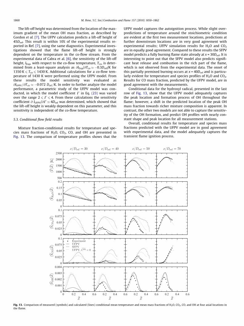
Mixture fraction-conditional results for temperature and spe-cies mass fractions of H2O, CO2, CO, and OH are presented inFig. 13. The comparison of temperature profiles shows that the

Fig. 13. Comparison of measured (symbols) and calculated (lines) conditional mean temthe flame.

UFPV model captures the autoignition process. While slight over-predictions of temperature around the stoichiometric conditionare evident at the first two measurement locations, predictions atfurther downstream locations are in very good agreement withexperimental results; UFPV simulation results for H2O and CO2

are in equally good agreement. Compared to these results the SFPVmodel predicts a fully burning flame state already at x = 30Dref. It isinteresting to point out that the SFPV model also predicts signifi-cant heat release and combustion in the rich part of the flame,which is not observed from the experimental data. The onset ofthis partially premixed burning occurs at x = 40Dref and is particu-larly evident for temperature and species profiles of H2O and CO2.Results for CO mass fraction, predicted by the UFPV model, are ingood agreement with the measurements.

Conditional data for the hydroxyl radical, presented in the lastrow of Fig. 13, show that the UFPV model adequately capturesthe peak location and formation process of OH throughout theflame; however, a shift in the predicted location of the peak OHmass fraction towards richer mixture composition is apparent. Incontrast, the other two models are not able to capture the sensitiv-ity of the OH formation, and predict OH profiles with nearly con-stant shape and peak location for all measurement stations.

Overall, conditional results for temperature and species massfractions predicted with the UFPV model are in good agreementwith experimental data, and the model adequately captures thetransient flame ignition process.

perature and mean mass fractions of H2O, CO2, CO, and OH at four axial locations in

Fig. 14. PDF of the flame stabilization point. The dashed lines correspond toisocontours of the mean mixture fraction with feZg ¼ f0:01;0:05;0:177g (from topto bottom), and the solid lines denote the mean axial and radial locations of thestabilization point.

Fig. 15. PDF of the flame index FI, evaluated at the flame stabilization point.

M. Ihme, Y.C. See / Combustion and Flame 157 (2010) 1850–1862 1861

5.4. Flamebase analysis

In this section, the structure and the stabilization mechanism atthe flamebase are analyzed. To identify the autoignition events atthe flamebase, associated with the formation of OH through theconsumption of intermediate HO2 species, an isocontour of theOH mass fraction with eY OH ¼ 10�3 has been selected. This criterionis identical to that used in Ref. [2], and our analysis showed thatthis marker is adequate in identifying the onset of ignition at theflamebase. With this, the flamebase is identified as the most up-stream location of this isocontour, and the simulation results aresampled to extract this stabilization point. The PDF for the stabil-ization location is shown in Fig. 14. The dashed lines correspondto three isocontours of the mean mixture fraction withfeZg ¼ f0:01;0:05;0:177g; and the solid lines denote the mean axialand radial locations of the stabilization point. From this statisticalanalysis it can been seen that the stabilization point, defined by thecriterion above, is confined to the fuel lean region. While theflamebase fluctuations are confined to a relatively narrow regionin radial direction, considerable variations in axial direction areapparent. In addition, statistical results of Fig. 14 suggest that theflame stabilizes at three preferred locations, that are indicated bythe white symbols. An analysis of the flow field structure showedthat the scalar dissipation rate at the stabilization point is belowthe critical value at ignition, which is consistent with the scatterplot shown in Fig. 8.

To characterize the combustion mode at the stabilization loca-tion, the flame index [38] is evaluated. The flame index FI, quanti-fies the alignment between the fuel and oxidizer gradients, and ishere defined as

FI ¼reY CH4 � reY O2 � YF

O2reZ�

jreY CH4 j reY O2 � YFO2reZ� ; ð33Þ

in which eY CH4 and eY O2 are obtained from the UFPV chemistry table,and the term Y F

O2reZ is subtracted to account for the oxygen in the

fuel stream. A value of FI = �1 defines a diffusion mode and FI = 1corresponds to the premixed autoignition regime.

The PDF of the flame index, evaluated at the stabilization point,is shown in Fig. 15. These statistical results show that ignition oc-curs primarily in the diffusion mode, and a quantitative analysisshowed that 50% of all ignition events occur under conditions inwhich the alignment angle between fuel and oxidizer gradients ex-ceeds 3/4p. The result that the stabilization location is primarilycontrolled by non-premixed conditions is in agreement with previ-ous DNS-studies [2,39].

6. Conclusions

An unsteady flamelet/progress variable model has been devel-oped for the prediction of autoignition in turbulent lifted flames.The model is a consistent extension to the steady flamelet/progressvariable approach, and employs an unsteady flamelet formulationto describe the transient evolution of all thermochemical quanti-ties during the flame ignition process. In this UFPV model, all ther-mochemical quantities are parameterized by mixture fraction,reaction progress parameter, and stoichiometric scalar dissipationrate. The particular advantage of the UFPV model over previouslydeveloped unsteady flamelet formulations is that in this modelthe flamelet time is replaced by physical quantities, which leadsto significant simplifications in computation and parameterizationof the thermodynamic state space. The UFPV model was analyzedin an a priori study to assess underlying modeling assumptions thatarise from the population of the state space.

A presumed PDF closure model is employed to evaluate Favre-averaged thermochemical quantities. For this a beta-distributionis used for the mixture fraction, a statistically most-likely distribu-tion is employed for the reaction progress parameter, and the dis-tribution of the stoichiometric scalar dissipation rate is modeled bya Dirac delta function.

The UFPV model was applied in LES of a lifted flame in a vitiatedco-flow, and simulation results are compared with experimentaldata. Additional calculations with the SFPV model and a modifiedUFPV formulation are carried out to investigate transient effectsand to quantify the significance of turbulence/chemistry interac-tion a posteriori. Simulation results show that the UFPV modelleads to significantly improved predictions of flame structure,lift-off height, and spatiotemporal evolution of the flow field.Although the UFPV model predicts a slightly faster ignition behav-ior, statistical results for mixture fraction, temperature, and speciesare in good agreement with experimental data. In contrast, theSFPV model results in a significantly faster ignition process thatis not in agreement with the experimental results. Furthermore,the importance of turbulence/chemistry interaction was analyzed,and it was shown that by neglecting subgrid fluctuations of theprogress variable the UFPV model predicts an extended ignitionregion.

Mixture fraction-conditional data for temperature and speciesmass fractions of H2O,CO2,CO, and OH are analyzed and comparedwith experimental results. In addition, scatter plots show that theUFPV model occupies a large portion of the unsteady flameletspace, while the scatter data for the SFPV model give a much fasterignition process, which is consistent with the findings from the apriori study. The SFPV results also show that the predicted flamestates are primarily confined to the upper stable branch of the S-shaped curve, which explains the short ignition time and reductionin the lift-off height.

For future work it would be interesting to also account for scalardissipation fluctuations in the presumed PDF closure. It is antici-pated that the statistical consideration of these subgrid scale fluc-tuations would further improve the simulation results of the UFPVmodel.

1862 M. Ihme, Y.C. See / Combustion and Flame 157 (2010) 1850–1862

Acknowledgment

The authors gratefully acknowledge financial support throughthe Office of Naval Research under Contract No. N00014-10-1-0561 with Dr. H. Scott Coombe as technical monitor.

References

[1] A.H. Lefebvre, Gas Turbine Combustion, Taylor & Francis, New York, 1999.[2] C.S. Yoo, R. Sankaran, J.H. Chen, J. Fluid Mech. 640 (2009) 453–481.[3] H. Pitsch, Ann. Rev. Fluid Mech. 38 (2006) 453–482.[4] H. Pitsch, M. Ihme, An unsteady/flamelet progress variable method for LES of

nonpremixed turbulent combustion, AIAA Paper 2005-557, 2005.[5] H. Pitsch, H. Steiner, Phys. Fluids 12 (10) (2000) 2541–2554.[6] R. Cabra, J.-Y. Chen, R.W. Dibble, A.N. Karpetis, R.S. Barlow, Combust. Flame 143

(2005) 491–506. <http://www.me.berkeley.edu/cal/vcb/data/VCMAData.html>.[7] R.L. Gordon, A.R. Masri, S.B. Pope, G.M. Goldin, Combust. Flame 151 (2007)

495–511.[8] K. Gkagkas, R.P. Lindstedt, Proc. Combust. Inst. 31 (2007) 1559–1566.[9] P. Domingo, L. Vervisch, D. Veynante, Combust. Flame 152 (2008) 415–432.

[10] J.-B. Michel, O. Colin, C. Angelberger, D. Veynante, Combust. Flame 156 (2009)1318–1331.

[11] M. Germano, U. Piomelli, P. Moin, W.H. Cabot, Phys. Fluids A 3 (7) (1991)1760–1765.

[12] D.K. Lilly, Phys. Fluids A 4 (3) (1992) 633–635.[13] S. Ghosal, J. Comput. Phys. 125 (1) (1996) 187–206.[14] C.D. Pierce, P. Moin, J. Fluid Mech. 504 (2004) 73–97.[15] M. Ihme, C.M. Cha, H. Pitsch, Proc. Combust. Inst. 30 (2005) 793–800.[16] N. Peters, Prog. Energy Combust. Sci. 10 (3) (1984) 319–339.[17] N. Peters, Combust. Sci. Technol. 30 (1983) 1–17.

[18] N. Peters, Turbulent Combustion, Cambridge University Press, Cambridge,2000.

[19] M. Ihme, H. Pitsch, Phys. Fluids 20 (2008) 055110.[20] A. Liñán, A. Crespo, Combust. Sci. Technol. 14 (1–3) (1976) 95–117.[21] C. Wall, B.J. Boersma, P. Moin, Phys. Fluids 12 (10) (2000) 2522–2529.[22] J. Jiménez, A. Liñán, M.M. Rogers, F.J. Higuera, J. Fluid Mech. 349 (1997) 149–

171.[23] E.T. Jaynes, Phys. Rev. 106 (4) (1957) 620–630.[24] C.H. Shannon, Bell System Technol. J. 27 (3) (1948) 379–423.[25] I.J. Good, Ann. Math. Stat. 34 (3) (1963) 911–934.[26] S.B. Pope, J. Non-Equilib. Thermodyn. 4 (1979) 309–320.[27] C.-S. Fang, J.R. Rajasekera, H.-S.J. Tsao, Entropy Optimization and Mathematical

Programming, Kluwer Academic Publisher, Boston, 1997.[28] M. Ihme, H. Pitsch, Combust. Flame 155 (2008) 90–107.[29] T. Poinsot, D. Veynante, Theoretical and Numerical Combustion, R.T. Edwards,

Inc., Philadelphia, PA, 2001.[30] R.O. Fox, Computational Models for Turbulent Reacting Flows, Cambridge

University Press, Cambridge, 2003.[31] M. Ihme, Pollutant formation and noise emission in turbulent non-premixed

flames, PhD thesis, Stanford University, 2007.[32] C.M. Cha, P. Trouillet, Phys. Fluids 15 (6) (2003) 1375–1380.[33] M. Ihme, Y.C. See, Large-eddy simulation of a turbulent lifted flame in a

vitiated co-flow, AIAA Paper 2009-239, 2009.[34] C.T. Bowman, R.K. Hanson, D.F. Davidson, W.C. Gardiner, V. Lissianski, G.P.

Smith, D.M. Golden, M. Frenklach, M. Goldenberg, GRI-Mech 2.11, 1997,<http://www.me.berkeley.edu/gri-mech/>.

[35] H. Pitsch, FLAMEMASTER V3.1: a C++ computer program for 0D combustion and 1Dlaminar flame calculations, 1998, <http://www.stanford.edu/group/pitsch/>.

[36] H. Pitsch, M. Chen, N. Peters, Proc. Combust. Inst. 27 (1998) 1057–1064.[37] R.L. Gordon. A Numerical and Experimental Investigation of Autoignition. PhD

thesis, University of Sydney, 2008.[38] H. Yamashita, M. Shimada, T. Takeno, Proc. Combust. Inst. 26 (1996) 27–34.[39] P. Domingo, L. Vervisch, J. Réveillon, Combust. Flame 140 (2005) 172–195.