Embed Size (px)
Citation preview
The Pennsylvania State University
The Graduate School
Department of Civil and Environmental Engineering
PREDICTION OF CONSOLIDATION TIMES FOR SHEAR STRENGTH
TESTING OF GEOSYNTHETIC CLAY LINERS USING CS2 MODEL
A Thesis in
Civil Engineering
by
Chu Wang
©2016 Chu Wang
Submitted in Partial Fulfillment
of the Requirements
for the Degree of
Master of Science
December 2016
ii
The thesis of Chu Wang was reviewed and approved* by the following:
Patrick J. Fox
John A. and Harriette K. Shaw Professor
Head of the Department of Civil and Environmental Engineering
Thesis Advisor
Tong Qiu
Associate Professor of Civil and Environmental Engineering
Ming Xiao
Associate Professor of Civil and Environmental Engineering
*Signatures are on file in the Graduate School

iii
ABSTRACT
The objectives of this study were to investigate the consolidation behavior and
predict consolidation times for shear strength testing of geosynthetic clay liners
(GCLs). These objectives were achieved by performing a series of numerical
simulations using the numerical model CS2 (Fox and Berles 1997; Fox and Pu 2012).
GCL consolidation was assessed for three values of initial overburden stress (10 kPa,
100 kPa and 1000 kPa), six load increment ratios (LIRs) (0.25, 0.5, 0.75, 1.0, 1.25,
1.5), double-drained (DD) and single-drained (SD) conditions, and two values of
specific gravity (1.0 and 2.21). Constitutive relationships for GCL compressibility
and hydraulic conductivity were taken from experimental data published by Kang and
Shackelford (2010).
Values of consolidation times 𝑡50, 𝑡70, 𝑡90, 𝑡95, and 𝑡98 are presented for
various conditions and plotted versus LIR. Consolidation times for both DD and SD
conditions decrease as LIR increases for a given initial overburden stress, and these
times decrease as initial overburden stress increases at a given LIR. The longest
predicted time required for 98% GCL consolidation and SD conditions is 32.5 h,
which corresponds to low initial stress and low LIR. Thus, for a direct shear test, the
recommended consolidation time for a GCL prior to the start of shearing is 48 h for
single-drainage. The longest predicted time required for 98% GCL consolidation
and DD conditions is 8.1 h, which also corresponds to low initial stress and low LIR.
Thus, the recommended consolidation time for a GCL prior to the start of shearing is
24 h or overnight for double-drainage.

iv
This study found that the ratios of consolidation times for DD to SD conditions
are approximately equal to 4.0 in all cases, which is consistent with classical
consolidation theory. Numerical solutions obtained for 𝐺𝑠 = 1 are nearly identical
to corresponding solutions obtained for 𝐺𝑠 = 2.21. This indicates the effect of self-
weight of GCL solids is negligible, which is consistent with GCLs being very thin
materials.
v
Table of Contents
List of Figures .............................................................................................................. vii
List of Tables ............................................................................................................. viii
Acknowledgements ....................................................................................................... ix
Chapter 1 Introduction ................................................................................................... 1
1.1 Geosynthetic Clay Liners ..................................................................................... 1
1.2 Numerical Modeling Approach ............................................................................ 3
1.3 Research Objectives ............................................................................................. 4
1.4 Outline .................................................................................................................. 5
Chapter 2 Literature Review .......................................................................................... 6
2.1 GCL Products ....................................................................................................... 6
2.2 Direct Shear Test Procedure ................................................................................. 8
2.3 Direct Shear Device ............................................................................................. 9
2.4 Effect of Consolidation ...................................................................................... 11
Chapter 3 CS2 Model Description ............................................................................... 14
3.1 Model Geometry ................................................................................................ 14
3.2 Constitutive Relationships .................................................................................. 15
3.3 Model Formulation ............................................................................................. 17
3.4 Computational Procedures ................................................................................. 23
3.5 Model Performance ............................................................................................ 26
Chapter 4 GCL Consolidation Times for Shear Strength Testing ............................... 29
4.1 GCL Consolidation Properties ........................................................................... 29
4.2 Model Input Data and Simulation Arrangements .............................................. 32
4.3 Consolidation Times for GCLs .......................................................................... 35
4.4 Ratio of Consolidation Times for DD and SD Conditions ................................. 43
4.5 Comparison of Solutions for 𝐺𝑠 = 1 and 𝐺𝑠 = 2.21 ....................................... 47
Chapter 5 Conclusions and Future Research ............................................................... 49

vi
5.1 Conclusions ........................................................................................................ 49
5.2 Future Research .................................................................................................. 50
References .................................................................................................................... 52
Appendices ................................................................................................................... 59

vii
List of Figures
Figure 1-1. GCL installation on side slope of a bottom liner system ............................ 2
Figure 2-1. GCL products .............................................................................................. 6
Figure 2-2. Cross section of large direct shear machine (Fox et al. 2006) .................. 11
Figure 2-3. Cross section of the test chamber for large direct shear machine (Fox et al.
2006) ..................................................................................................................... 11
Figure 2-4. Peak and residual failure envelops for a GCL hydrated at the shearing
normal stress (Eid and Stark 1997) ....................................................................... 12
Figure 2-5. Peak and residual failure envelops for a GCL hydrated at a normal stress
of 17 kPa and then consolidated to the shearing normal stress (Eid and Stark
1997) ..................................................................................................................... 13
Figure 3-1. CS2 model geometry: (a) initial configuration; (b) configuration after
application of vertical stress (Fox and Pu 2012) .................................................. 15
Figure 3-2. Constitutive relationships: (a) compressibility relationship; (b) hydraulic
conductivity relationship (Fox and Pu 2012)........................................................ 17
Figure 3-3. Schema of fluid flows (modified from Fox and Berles 1997) .................. 21
Figure 3-4. Flow chart for CS2 (Fox and Berles 1997) ............................................... 25
Figure 3-5. Loading sequence for time-dependent loading example (Fox and Pu 2012)
.............................................................................................................................. 27
Figure 4-1. Compressibility relationship for GCLs (Kang and Shackelford 2010) ..... 31
Figure 4-2. Hydraulic conductivity relationship for GCLs (Kang and Shackelford
2010) ..................................................................................................................... 32
Figure 4-3. Consolidation data for DD GCLs: (a) 𝑡50 and 𝑡90; (b) 𝑡95 and 𝑡98 ...... 39
Figure 4-4.Consolidation data for SD GCLs: (a) 𝑡50 and 𝑡90; (b) 𝑡95 and 𝑡98 .......... 42
Figure 4-5. Time ratios of SD to DD versus LIR: (a) 𝑡50 and 𝑡90; (b) 𝑡95 and 𝑡98 ... 46

viii
List of Tables
Table 3-1. Comparison of CS2 results with analytical solutions for time-depending
loading (Fox and Pu 2012) ................................................................................... 28
Table 4-1. Initial GCL thicknesses and void ratios for three values of initial
overburden stress .................................................................................................. 33
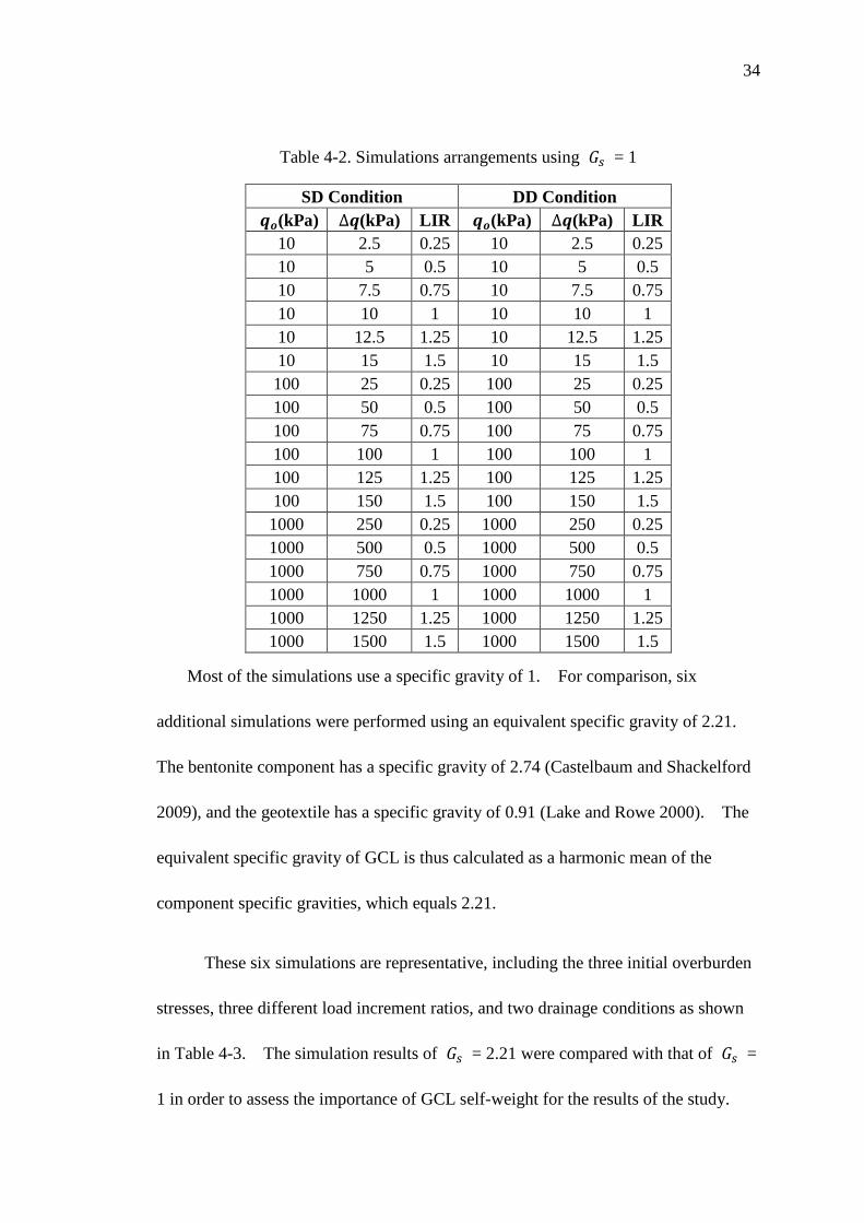
Table 4-2. Simulations arrangements using 𝐺𝑠 = 1 ................................................... 34
Table 4-3. Simulation arrangements using 𝐺𝑠 = 2.21 for comparison ...................... 35
Table 4-4. Consolidation times for GCL with DD condition ...................................... 37
Table 4-5. Consolidation times for GCL with SD condition ....................................... 38
Table 4-6. Ratios of consolidation times of SD GCLs to DD GCLs ........................... 45
Table 4-7. Comparison of simulation results for 𝐺𝑠 = 2.21 and 𝐺𝑠 = 1 .................. 48
ix
Acknowledgements
Firstly, I would like to express my deepest gratitude to my advisor, Prof. Patrick
Fox, who not only has immense knowledge but also has a charming personality. His
timely advice, scientific approach, meticulous scrutiny, unwavering encouragement,
patient guidance and financial support have proved invaluable in helping me to
accomplish this task and in helping me to grow as a student and as a researcher on a
tremendous scale.
Additionally, my sincere thanks go to the thesis committee members, who are
also my instructors, Prof. Tong Qiu and Prof. Ming Xiao, for their knowledge,
expertise, guidance, and all the additional help and support they have provided me
with on this study. I am also truly grateful to Prof. Hefu Pu, who has provided me
with a great deal of knowledge and technical support regarding CS2. In addition, I
would like to thank the faculty and staff at the Department of Civil and Environmental
Engineering for all of their tireless efforts, time, and assistance.
Last, but certainly not least, I would like to thank my friends and especially my
parents. Their unconditional, selfless love and support is the cornerstone of all of
my accomplishments. None of this would have been possible without them.

1
Chapter 1
Introduction
1.1 Geosynthetic Clay Liners
In the last 25 years, geosynthetic clay liners have been widely utilized as
hydraulic barriers in a large number of waste containment facilities and other
engineering applications. As part of a composite liner, GCLs are typically placed at
the bottom of landfills, as shown in Fig.1-1, or in cover system. A primary concern
for such applications is the static and seismic stability of slopes that incorporate
GCLs. This is because bentonite, the major component of a GCL, has low shear
strength after hydration. GCLs also display variability in shear strength due to the
variability of component materials and changes in GCL design and testing over years.
As a result, internal and interface shear strengths of GCLs must be measured on a
routine basis and detailed technical specifications have been developed for such tests
(e.g., ASTM D 6243).
2
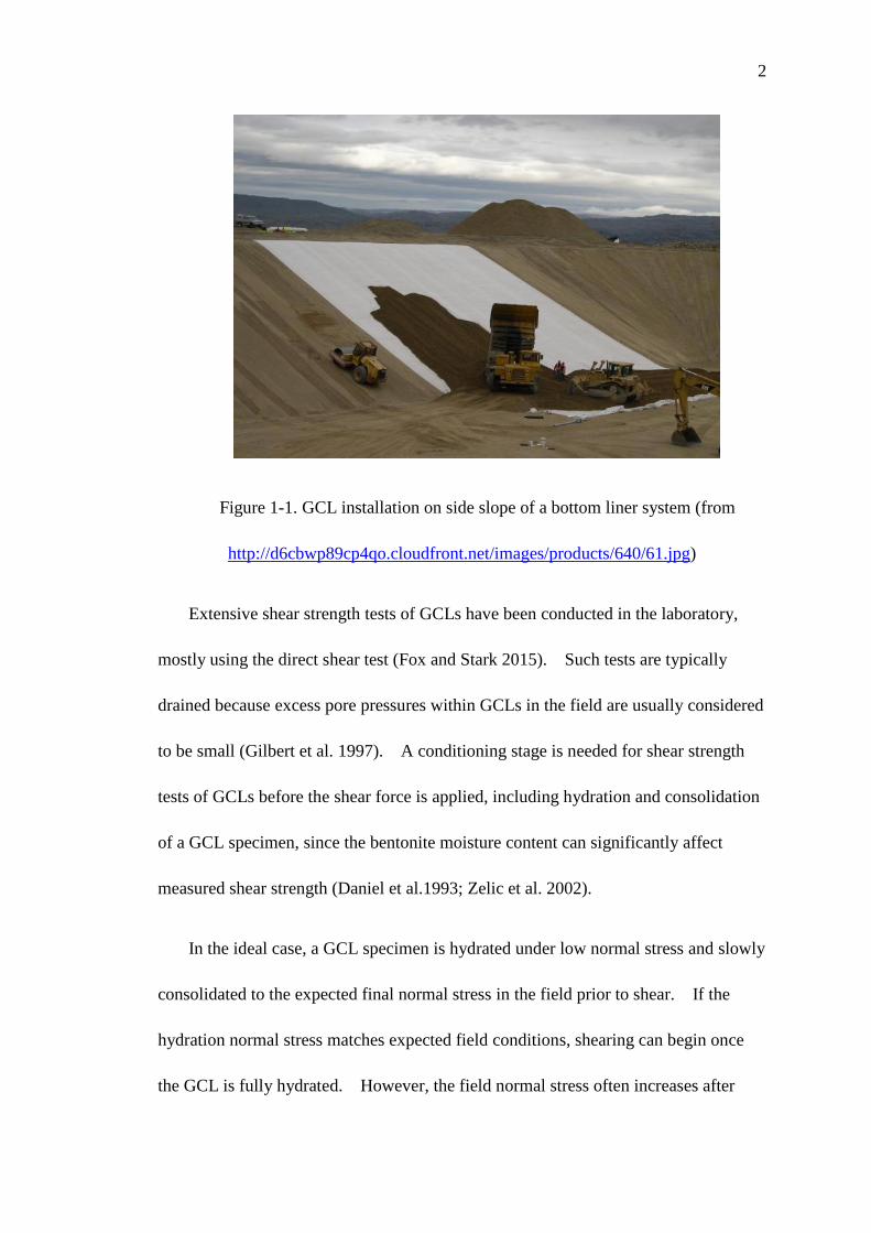
Figure 1-1. GCL installation on side slope of a bottom liner system (from
http://d6cbwp89cp4qo.cloudfront.net/images/products/640/61.jpg)
Extensive shear strength tests of GCLs have been conducted in the laboratory,
mostly using the direct shear test (Fox and Stark 2015). Such tests are typically
drained because excess pore pressures within GCLs in the field are usually considered
to be small (Gilbert et al. 1997). A conditioning stage is needed for shear strength
tests of GCLs before the shear force is applied, including hydration and consolidation
of a GCL specimen, since the bentonite moisture content can significantly affect
measured shear strength (Daniel et al.1993; Zelic et al. 2002).
In the ideal case, a GCL specimen is hydrated under low normal stress and slowly
consolidated to the expected final normal stress in the field prior to shear. If the
hydration normal stress matches expected field conditions, shearing can begin once
the GCL is fully hydrated. However, the field normal stress often increases after

3
hydration, and the shear strength at a higher normal stress condition is required. In
this case, consolidation of a GCL test specimen to the desired normal stress is
necessary to obtain this shear strength. As with natural soils, GCL shear strengths
are a function of the effective normal stress acting on the failure plane, and a GCL
specimen that is not fully consolidated prior to shearing may yield low shear strength
due to the presence of excess pore pressures (McCartney et al. 2009; Fox and Stark
2015).
Many studies have been conducted to investigate internal and interface shear
strengths for GCLs; however, the long time required for GCL consolidation often
influences the practicality of such tests. Some laboratories use accelerated schedules
to avoid long testing times, with the GCL consolidation period as short as a couple of
hours. The consolidation behavior of natural soils has been widely studied, but
almost no similar work has been conducted for GCLs. This thesis presents a
numerical investigation of the consolidation behavior for GCLs and provides
predictions and recommendations for consolidation times for shear strength testing of
GCLs.
1.2 Numerical Modeling Approach
Soil consolidation has been one of the oldest analysis methods in geotechnical
engineering and a large number of theories and numerical models have been
developed. Fox and Berles (1997) first published a piecewise-linear model for 1D
large strain consolidation, called Consolidation Settlement 2 (CS2). Fox and Pu
(2012) published an updated and enhanced version of CS2. The CS2 modeling

4
approach has been extensively used and validated since these original publications,
and thus, CS2 was utilized to conduct numerical simulations of GCL consolidation
behavior in this study.
In the CS2 method, all variables pertaining to geometry, material properties, fluid
flow, and effective stress are updated at each time step with respect to a fixed
coordinate system. This method is a Lagrangian approach that follows the motion of
the solid phase throughout the consolidation process. In subsequent studies, the
method has been adapted to accommodate accreting layers (Fox 2000), radial and
vertical flows (Fox et al. 2003), compressible pore fluid (Fox and Qiu 2004), high-
gravity conditions in geotechnical centrifuge (Fox et al. 2005), and coupled solute
transport (Fox 2007a; Fox and Lee 2008). The original CS2 model takes into
consideration “vertical strain, soil self-weight, general constitutive relationships,
relative velocity of fluid and solid phases, and changing hydraulic conductivity and
compressibility during the consolidation process. Fox and Pu (2012) then
incorporated several new capabilities into the model, including time-dependent
loading, an external hydraulic gradient acting across the consolidating layer, and
unload/reload effects.”
1.3 Research Objectives
The primary objectives of this research study were to investigate the
consolidation behavior and provide recommendations for consolidation times for
shear strength testing of GCLs, by numerically simulating the consolidation process.
The CS2 model was utilized to achieve these research objectives.

5
1.4 Outline
This thesis is divided into five chapters. Chapter 1 presents the background
information, research objectives and thesis outline. Chapter 2 summarizes the
existing literature associated with shear strength testing of GCLs and the CS2
numerical model. Chapter 3 describes the CS2 model, including assumptions, main
procedures, capabilities, and verification checks. Chapter 4 presents an analysis of
numerical simulations for GCL consolidation under various conditions. Chapter 5
presents conclusions and recommendations from this study and suggestions for future
research.

6
Chapter 2
Literature Review
2.1 GCL Products
GCLs are manufactured products composed of a layer of bentonite clay enclosed
by one or more layers of geosynthetic materials, as shown in Fig. 2-1. Fox and Stark
(2015) described several types of GCL products, which can be generally categorized
into unreinforced and reinforced GCLs. Unreinforced GCLs can be installed at
facilities where the slope instability is less likely to occur, whereas reinforced GCLs
are able to transfer applied shear stress into tensile stress on the internal reinforcement
fibers to provide much greater shear strength (Zornberg and McCartney 2009).
Figure 2-1. GCL products (from
http://www.exportersindia.com/gorantlageosyntheticspvtltd/products.htm#geosyntheti
c-clay-liner-chennai-india-1384768)

7
Unreinforced GCLs typically contain a layer of sodium bentonite affixed to a
geotextile or geomembrane, and there is no reinforcement traversing the bentonite
layer. Unreinforced GCLs essentially have the same shear strength as bentonite.
Adhesives and moisture may be mixed in the bentonite layer in order to prevent
bentonite from being lost when the GCL is transported and installed. The geotextiles
supporting the bentonite layer for unreinforced GCLs can be woven or nonwoven.
When the bentonite layer is affixed to one side of a smooth or textured geomembrane,
it is considered as geomembrane-supported unreinforced GCL. In addition,
encapsulated GCLs are constructed by an unreinforced geomembrane-supported GCL
and a second geomembrane over this GCL. The purpose of this design is to keep the
bentonite dry and thereby significantly increase the peak and residual shear strength.
Reinforced GCLs contain geosynthetic reinforcement that passes through the
bentonite layer to greatly increase the shear strength of the product. As described by
Fox and Stark (2015), two primary reinforcement methods for geotextile-supported
GCLs are stitch-bonding and needle-punching. Stitched-bonded GCLs contain a
layer of bentonite between two geotextiles sewn together by parallel lines of stitching.
Needle-punched GCLs contain reinforcing fibers that are pulled from a nonwoven
geotextile, across the bentonite layer, and imbedded in a woven or nonwoven carrier
geotextile. Additionally, reinforced GCLs can also be encapsulated between two
textured geomembranes, which is becoming a more frequent choice for waste
containment design. In this case, bentonite not only has higher shear strength due to

8
the presence of reinforcement but is also protected against hydration (Fox and Stark
2015).
In addition, there are other types of GCLs that have been developed for a
diversity of applications, including GCLs with an internal structure similar to a
geonet, heat-treated needle-punched GCLs, and composite laminate GCLs (Fox and
Stark 2015). Furthermore, polymer-amended bentonites have been developed for
designs where ion exchange leads to much higher hydraulic conductivity for natural
bentonite GCLs (Trauger and Darlington 2000).
2.2 Direct Shear Test Procedure
Although more appropriate for measurement of GCL shear strength, long-term
tests are seldom conducted due to large costs and difficulties in procedure. Instead,
short-term tests are employed in the design of facilities that utilize GCLs as hydraulic
barriers (Fox and Stark 2015). Most short-term shear strength tests for GCLs are
conducted by direct shear, though some alternatives, such as the ring shear test and tilt
table test, are occasionally used (Marr 2001).
ASTM D6243 specifies the current standard test method for determining the
internal and interface shear strengths of geosynthetic clay liners by the direct shear
method. The minimum specimen dimension is 300 mm, with square and rectangular
specimens recommended. The gripping surface and clamps should secure the test
specimen tightly and not interfere with measured shear strength. Textured shearing
surfaces should be rough enough for internal strength tests, and if possible, should be

9
rigid and allow free water to flow into and out of the specimen. Test procedures
include specimen configuration, soil compaction criteria, specimen conditioning
(hydration, consolidation), normal stress level, method of shearing and shear
displacement rate. These procedures are specified by users. The minimum shear
displacement is 50 mm. Shearing can be displacement-controlled or stress-
controlled. Stress-controlled methods include constant stress rate, incremental
stress, and constant stress creep. Displacement control is required to measure post-
peak response. Correction for measured shear force is required due to machine
friction. A shearing rate of 1 mm/min is allowed if excess pore pressures are not
expected to develop on the failure surface. After a test is finished, the user should
inspect the failed specimen and record the mode of failure (Fox et al 2004).
2.3 Direct Shear Device
The direct shear test for measurements of GCL shear strength has several
advantages (Fox and Stark 2015). Firstly, shear occurs in one direction to match
field condition, and this is necessary to GCLs and GCL interfaces that display in-
plane anisotropy. Secondly, the direct shear device can accommodate large
specimen size. Lastly, shear deformation produced by the direct shear test is
relatively uniform, which tends to minimize progressive failure effects and allows for
accurate measurements of peak shear strength. However, there are also some
limitations. The maximum shearing displacement of standard direct shear device is
generally not enough for measurements of residual shear strength. The shear failure

10
surface area decreases during shear, which increases the shearing normal stress, and
thus a correction for area of failure surface is required for data analysis.
A direct shear machine for relatively large specimens was developed by Fox et al.
(1997). This device allows for a specimen dimension of 406 mm 1067 mm, large
displacement of 203 mm, large range of displacement rate, and negligible machine
friction and more effective specimen gripping surfaces.
Fox et al. (2006) further refined the design of the original direct device to
accommodate both static and dynamic shear testing. Fig. 2-2 shows a profile view
of the 2006 device and Fig. 2-3 shows the test chamber in detail. This device allows
for specimen size of 305 mm ×1067 mm and thickness up to 250 mm, and has a
maximum horizontal displacement of 254 mm, a maximum normal stress capacity of
2000 kPa and maximum shear stress capacity of 750 kPa. The specimen gripping
system consists of 305 mm ×305 mm modified metal connected plates, with 864
triangular teeth extruding from one side. The gripping ability is sufficient to prevent
slippage so that clamps are often unnecessary for internal GCL shear tests. This
gripping system allows a specimen so shear on the weakest plane with minimal
progressive failure effect (Fox et al. 2006; Fox and Kim 2008). The minimum
displacement rate is 0.01 mm/min., and the maximum sustained sinusoidal frequency
is 4 Hz with an amplitude of 25 mm. The friction coefficient of this machine is
reported as 0.27%.

11
Figure 2-2. Cross section of large direct shear machine (Fox et al. 2006)
Figure 2-3. Cross section of the test chamber for large direct shear machine (Fox
et al. 2006)
2.4 Effect of Consolidation
Eid and Stark (1997) compared the peak and residual strengths of encapsulated
GCLs with those of identical specimens that were hydrated and consolidated prior
shearing. Fig. 2-4 shows peak and residual strength envelops for five encapsulated
GMX/GM-supported GCL specimens that were hydrated at shearing normal stress.
Fig 2-5 shows peak and residual strength envelops for replicate specimens that were

12
hydrated at a normal stress of 17 kPa and then consolidated to the shearing normal
stress. Eid and Stark (1997) found a 25% to 30% strength reduction for the
consolidated specimens. Hydration at low normal stress leads to more water
absorption, more particle rearrangement, and larger bentonite expansion, but some of
this water was not expelled during the following consolidation. Thus, these
consolidated specimens had larger water content (Eid and Stark 1997) and internal
shear strength of unreinforced GCLs decreases with an increase of bentonite water
content (Daniel et al. 1993; Zelic et al. 2002).
Figure 2-4. Peak and residual failure envelops for a GCL hydrated at the shearing
normal stress (Eid and Stark 1997)

13
Figure 2-5. Peak and residual failure envelops for a GCL hydrated at a normal
stress of 17 kPa and then consolidated to the shearing normal stress (Eid and Stark
1997)
The consolidation effect for reinforced GCLs has also been investigated.
McCartney et al. (2009) reported a reduction of internal peak shear strength for
needle-punched GCLs when the shear load was immediately applied after hydration
without consolidation. Excess pore pressures within the specimen may have
produced this reduction in internal peak strength.
Another effect of GCL specimen consolidation is that bentonite can extrude
through the geotextile if the load is applied too quickly, forming a slippery interface.
Bentonite extrusion can also lower interface shear strength with adjacent materials,
such as a geomembrane (Triplett and Fox 2001; Vukelic et al. 2008). Hewitt et al.
(1997) also indicated also insufficient consolidation could lead to shear strength
reduction for a geomembrane/GCL interface.
14
Chapter 3
CS2 Model Description
This chapter describes the CS2 model, including geometry in Section 3.1,
constitutive relationships in Section 3.2, formulation in Section 3.3, computational
procedures in Section 3.4, and performance in Section 3.5. More information
regarding CS2 can be found in Fox and Berles (1997) and Fox and Pu (2012).
3.1 Model Geometry
Model geometry for CS2 is described in Fox and Pu (2012). The initial
geometry of CS2, before the application of a vertical stress increment at time 𝑡 = 0,
is shown in Fig. 3-1(a). The configuration after the application of vertical stress
increment is shown in Fig. 3-1(b). Symbols and notations are provided in the
Appendices. The model assumes that a saturated compressible soil layer of initial
height, 𝐻𝑜, is regarded as an idealized two-phase material. The solid particles and
pore fluid in the material are assumed to be incompressible. The compressibility and
hydraulic conductivity constitutive relationships of the layer are homogeneous.
Vertical coordinate, 𝑧, is defined as positive upward from a fixed datum at the bottom
of the layer. Element coordinate, 𝑗, is also directed upward form the bottom
boundary, which is modified from the 1997 model. The layer is subdivided into a
column of 𝑅𝑗 elements, and each has unit cross-section area, constant initial height,
𝐿𝑜, and a central node located at initial elevation, 𝑧𝑜,𝑗. Nodes translate vertically
and remain at the center of respective elements throughout the consolidation process.
An initial effective overburden stress, 𝑞𝑜, is applied at the top boundary. Drainage

15
conditions (i.e. drained or undrained) for top and bottom boundaries can be specified
by the user. If drained conditions are specified, top and bottom boundaries are
assigned individual constant total head values, ℎ𝑡 and ℎ𝑏, taken with respect to the
datum. An external hydraulic gradient across the layer can be applied by assigning
different boundary head values. The distribution of initial void ratio, 𝑒𝑜,𝑗 can be
calculated by the CS2 model or provided by the user.
Figure 3-1. CS2 model geometry: (a) initial configuration; (b) configuration
after application of vertical stress (Fox and Pu 2012)
3.2 Constitutive Relationships
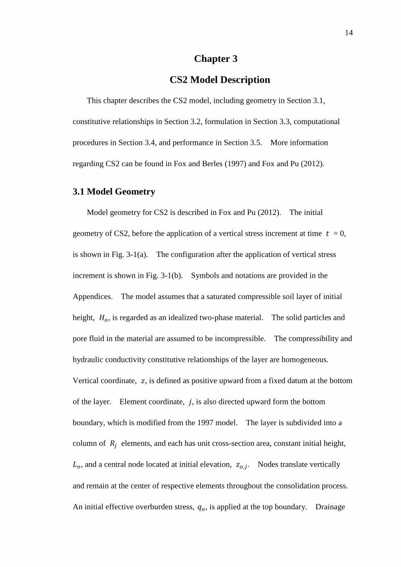
The constitutive relationships for CS2 are shown in Fig. 3-2, with each defined by
at least two pairs of data points. Fig. 3-2(a) shows the compressibility relationship.
The compressibility relationship is defined by data points representing void ratio
versus vertical effective stress. Values in between the data points are obtained by

16
linear interpolation. The compressibility relationship can also be defined using
equations. For the compressibility curve, normally consolidated or overconsolidated
conditions can be represented. Additionally, a user can also specify normally
consolidated or overconsolidated conditions by defining the compressibility
relationship. If the vertical effective stress for an element decreases below the
preconsolidation pressure, unloading/reloading follow an identical path defined by
𝜎𝑝,𝑗′𝑡 , 𝑒𝑝,𝑗
𝑡 and a constant recompression index 𝐶𝑟. Otherwise, the stress path will
follow the normally consolidation curve.
Fig. 3-2(b) shows the hydraulic conductivity relationship for the compressible
layer. The hydraulic conductivity relationship is defined by points representing
vertical hydraulic conductivity versus void ratio or can also be specified using
equations. The CS2 model uses the same hydraulic conductivity relationship for
both normally consolidated and overconsolidated conditions, which is consistent with
the data of Al-Tabbaa and Wood (1987), Nagaraj et al. (1994), and Fox (2007b).
17
Figure 3-2. Constitutive relationships: (a) compressibility relationship; (b)
hydraulic conductivity relationship (Fox and Pu 2012)
In Fig. 3-2, each void ratio uniquely corresponds to one vertical effective stress or
vertical hydraulic conductivity. Thus, the CS2 model does not account for effects of
strain rate, secondary compression, or aging on the compressibility or hydraulic
conductivity of the soil.
3.3 Model Formulation
The main computational procedures of the CS2 model include Node Elevations,
Stresses, Series Hydraulic Conductivity, Flow, Time Increment, Layer Settlement and
Degrees of Consolidation. Before running these procedures, the initial condition of
the soil layer is required. These initial calculations yield the distribution of initial
void ratio, ultimate (i.e., final) settlement of the soil layer, and distribution of final
void ratio in equilibrium with final stress conditions.

18
To start, the distribution of initial void ratio under initial effective overburden
stress 𝑞𝑜 is calculated by iteration. This distribution is in equilibrium with 𝑞𝑜, the
constitutive relationships and self-weight of soil, and seepage forces caused by an
external hydraulic gradient acting across the layer if ℎ𝑡 ≠ ℎ𝑏. At the top of the
layer, the initial vertical effective stress at the node of element 𝑅𝑗 , 𝜎′𝑜,𝑅𝑗, is estimated
as 𝑞𝑜, and the corresponding initial void ratio 𝑒𝑜,𝑅𝑗 of element 𝑅𝑗 is calculated
from the soil constitutive compressibility relationship shown in Fig. 3-2(a). This
void ratio is used to calculate the initial buoyant unit weight of the element, 𝛾′𝑜,𝑅𝑗.
For element 𝑅𝑗, the soil self-weight is the product of one-half of the constant element
initial thickness 𝐿𝑜
2 and the buoyant unit weight 𝛾′𝑜,𝑅𝑗
, since the node is located at the
center of the element. This gives a new value of vertical effective stress at the node
as:
𝜎′𝑜,𝑅𝑗 = 𝑞𝑜 +
𝐿𝑜
2(𝛾′𝑜,𝑅𝑗
− 𝑓𝑜,𝑅𝑗) (1)
where 𝑓𝑜,𝑅𝑗 = initial seepage force per unit weight (positive upward) acting on
element 𝑅𝑗. The first pass takes seepage forces on all elements as zero. An
updated value of 𝑒𝑜,𝑅𝑗 is calculated using 𝜎′𝑜,𝑅𝑗 based on the compressibility
relationship. This process is repeated until the 𝜎′𝑜,𝑅𝑗 in two successive iterations
are sufficiently close. Then, the effective stress at the top of element 𝑅𝑗 − 1 is
calculated as 𝜎′𝑜,𝑅𝑗−1 = 𝜎′𝑜,𝑅𝑗
+ 0.5𝐿𝑜 (𝛾′𝑜,𝑅𝑗− 𝑓𝑜,𝑅𝑗
). This process is then
repeated to calculate the effective stress at the nodes for the reaming elements.

19
If an external hydraulic gradient is applied (i.e. ℎ𝑏 ≠ ℎ𝑡), the iterative procedure
adds an additional loop for seepage forces. Once initial void ratios 𝑒𝑜,𝑗 are
calculated, the values of initial hydraulic conductivity 𝑘𝑜,𝑗 can be obtained from the
hydraulic conductivity relationship shown in Fig. 3-2(b). The steady discharge
velocity, 𝑣𝑜 through the layer (positive upward) is
𝑣𝑜 = ℎ𝑏 − ℎ𝑡
∑𝐿𝑜
𝑘𝑜,𝑗
𝑅𝑗
𝑗=1
(2)
and the corresponding seepage forces are
𝑓𝑜,𝑗 = 𝑣𝑜𝛾𝑤
𝑘𝑜,𝑗, 𝑗 = 1, 2, … , 𝑅𝑗 (3)
where 𝛾𝑤 = unit weight of water. Total stress on element 𝑗 is computed by
summing the initial overburden stress 𝑞𝑜, the overburden stress increment ∆𝑞𝑡 at
time 𝑡, the weight of water, the self-weight of element 𝑗 and the elements above
element 𝑗 as follows:
𝜎𝑡𝑗 = 𝑞𝑜 + ∆𝑞𝑡 + (ℎ𝑡 − 𝐻𝑡)𝛾𝑤 +
𝐿𝑡𝑗𝛾𝑡
𝑗
2+ ∑ 𝐿𝑡
𝑏𝛾𝑡𝑏
𝑅𝑗
𝑏=𝑗+1
, 𝑗 = 1, 2, . . . , 𝑅𝑗
(4)
The corresponding saturated unit weight of each element 𝛾𝑡𝑗 is
𝛾𝑡𝑗
= γw(𝐺𝑠 + 𝑒𝑗
𝑡)
1 + 𝑒𝑗𝑡 (5)
where 𝐺𝑠 = is the specific gravity of the soil layer, 𝑒𝑗𝑡 = corresponding void ratio.
Users specify a constant specific gravity for the entire layer. Layered systems, with
20
different 𝐺𝑠 values and different constitutive relationships for each layer, are treated
by the CS3 model (Fox et al. 2014).
The corresponding effective stress 𝜎𝑗′𝑡 at the node of element 𝑗 can be
calculated when the soil is overconsolidated (i.e. 𝑒𝑗𝑡 > 𝑒𝑚𝑖𝑛
𝑡 , where 𝑒𝑚𝑖𝑛𝑡 is the
corresponding preconsolidation void ratio).
𝜎′𝑡𝑗 = 𝜎′𝑡
𝑝,𝑗 𝑒𝑥𝑝 (2.303𝑒𝑡
𝑝,𝑗 − 𝑒𝑡𝑗
𝐶𝑟) , 𝑗 = 1, 2, . . . , 𝑅𝑗 (6)
𝜎′𝑡𝑗 can be also calculated from 𝑒𝑗
𝑡 by compressibility relationship shown in Fig. 3-
2(a), if 𝑒𝑗𝑡 ≤ 𝑒𝑚𝑖𝑛
𝑡 .
Once the vertical total stress 𝜎𝑡𝑗 and vertical effective stress σ′t
j for element 𝑗
are obtained, CS2 can calculate the pore pressure 𝑢𝑡𝑗 at the node of element 𝑗 as
𝑢𝑡𝑗 = 𝜎𝑡
𝑗 − 𝜎′𝑡𝑗 , 𝑗 = 1, 2, . . . , 𝑅𝑗 (7)
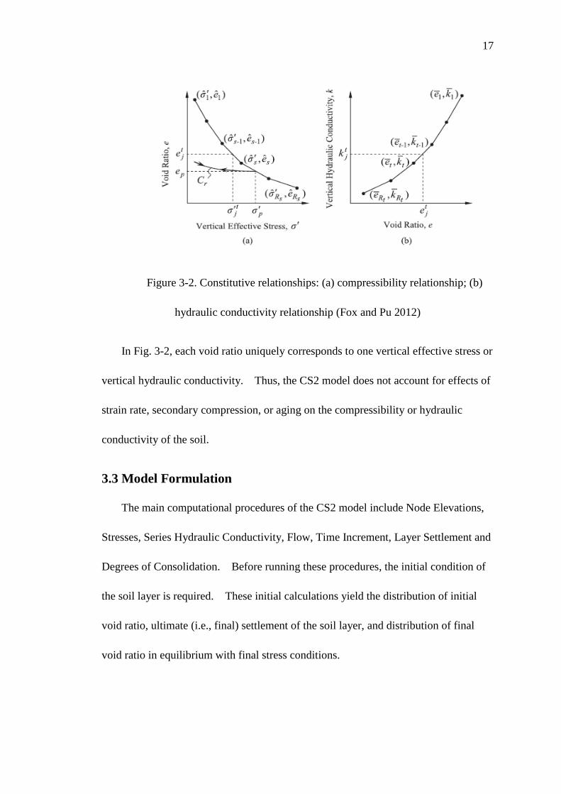
As shown in Fig. 3-3, the fluid flow between the nodes of element 𝑗 and element
𝑗 + 1 has a relative velocity 𝑣𝑡𝑟𝑓,𝑗 , traveling through two elements with different
hydraulic conductivities: 𝑘𝑡𝑗+1 in element 𝑗 + 1 and 𝑘𝑡
𝑗 in element 𝑗. The
corresponding relative discharge velocity 𝑣𝑡𝑟𝑓,𝑗 between element 𝑗 and element 𝑗 +
1 is
𝑣𝑡𝑟𝑓,𝑗 = −𝑘𝑡
𝑠,𝑗𝑖𝑡𝑗 , 𝑗 = 1, 2, . . . , 𝑅𝑗 − 1 (8)

21
where the hydraulic gradient 𝑖𝑡𝑗 between the node of element 𝑗 and 𝑗 + 1 is
𝑖𝑡𝑗 =
ℎ𝑡𝑗+1 − ℎ𝑡
𝑗
𝑧𝑡𝑗+1 − 𝑧𝑡
𝑗 , 𝑗 = 1, 2, . . . , 𝑅𝑗 − 1 (9)
and 𝑧𝑡𝑗 is the elevation at the node of element 𝑗.
Figure 3-3. Schema of fluid flows (modified from Fox and Berles 1997)
The total hydraulic head ℎ𝑡𝑗 at node 𝑗 is the sum of elevation head and pressure
head as
ℎ𝑡𝑗 = 𝑧𝑡
𝑗 +𝑢𝑡
𝑗
𝛾𝑤, 𝑗 = 1, 2, . . . , 𝑅𝑗 (10)
To compute the relative discharge velocity in Eqn. (8), the equivalent series
hydraulic conductivity 𝑘𝑡𝑠.𝑗 between the nodes of element 𝑗 and element 𝑗 + 1 is
required, which can be calculated as
22
𝑘𝑡𝑠.𝑗 =
𝑘𝑡𝑗+1𝑘𝑡
𝑗( 𝐿𝑡𝑗+1 + 𝐿𝑡
𝑗)
𝐿𝑡𝑗+1𝑘𝑡
𝑗 + 𝐿𝑡𝑗 𝑘𝑡
𝑗+1, 𝑗 = 1, 2, . . . , 𝑅𝑗 − 1 (11)
The element 𝑅𝑗 and element 1 should be specially considered, because these two
are respectively the top element and bottom element in the column, and the equations
shown above need to be modified for these two elements. If the top boundary is
undrained, the relative discharge velocity 𝑣𝑡𝑟𝑓,𝑅𝑗
at the top boundary is 0. Likewise,
if bottom boundary is undrained, the relative discharge velocity 𝑣𝑡𝑟𝑓,0 at the bottom
boundary is also 0. Otherwise, the relative discharge velocities are
𝑣𝑡𝑟𝑓,𝑅𝑗
= −𝑘𝑡𝑅𝑗
ℎ𝑡 − ℎ𝑡𝑅𝑗
𝐻𝑡 − 𝑧𝑡𝑅𝑖
(12)
𝑣𝑡𝑟𝑓,0 = −𝑘𝑡
1
ℎ𝑡1 − ℎ𝑏
𝑧𝑡1
(13)
Relative discharge velocities are used to calculate the net fluid outflow and can be
further used to calculate the change of element height. After a small time increment
of ∆𝑡, the corresponding new height of element 𝐿𝑗𝑡+∆𝑡 can be calculated as
𝐿𝑗𝑡+∆𝑡 = 𝐿𝑡
𝑗 − (𝑣𝑡𝑟𝑓,𝑗 − 𝑣𝑡
𝑟𝑓,𝑗−1)∆𝑡, 𝑗 = 1, 2, . . . , 𝑅𝑗 (14)
For this one-dimensional model, the element length is proportional to the void
ratio of the element. Hence, the new void ratio 𝑒𝑗𝑡+∆𝑡 for element 𝑗 over time
increment ∆𝑡 is
𝑒𝑗𝑡+∆𝑡 =
𝐿𝑗𝑡+∆𝑡(1 + 𝑒𝑜,𝑗)
𝐿𝑜− 1, 𝑗 = 1, 2, . . . , 𝑅𝑗 (15)
23
The new height of the entire layer 𝐻𝑡+∆𝑡 over time increment ∆𝑡 is the summation
of the lengths of all the elements as
𝐻𝑡+∆𝑡 = ∑ 𝐿𝑗𝑡+∆𝑡
𝑅𝑗
𝑗=1
(16)
The new settlement 𝑆𝑡+∆𝑡 is calculated by subtracting the new total layer
height 𝐻𝑡+∆𝑡 from the initial layer height 𝐻𝑜
𝑆𝑡+∆𝑡 = 𝐻𝑜 − 𝐻𝑡+∆𝑡 (17)
The average degree of consolidation over time increment ∆𝑡, is
𝑈𝑎𝑣𝑔𝑡+∆𝑡 =
𝑆𝑡+∆𝑡
𝑆𝑢𝑙𝑡 (18)
The time increment ∆𝑡 is chosen as the smaller value of:
∆𝑡 = 𝑚𝑖𝑛 {𝛼𝛾𝑤𝑎𝑣,𝑗
𝑡 (𝐿𝑗𝑡)
2
𝑘𝑗𝑡(1 + 𝑒𝑗
𝑡), |
0.01𝐿𝑜(𝑒𝑜,𝑗 − 𝑒𝑓,𝑗)
(1 + 𝑒𝑜,𝑗)(𝑣𝑡𝑟𝑓,𝑗 − 𝑣𝑡
𝑟𝑓,𝑗−1)|} (19)
where 𝛼 = 0.4, 𝑎𝑣,𝑗𝑡 = coefficient of compressibility for element j obtained from the
soil compressibility relationship, and 𝑒𝑓,𝑗 = final void ratio for element 𝑗. ∆t can
also be decreased to accommodate the loading schedule ∆𝑞𝑡 for the layer, which
forms a third constraint.
3.4 Computational Procedures
A flow chart is presented in Fig. 3-4 to demonstrate the basic algorithm for the
CS2 program. The required input data consists of maximum element number 𝑅𝑗,
the initial overburden stress 𝑞𝑜, time-dependent stress increment 𝛥𝑞, specific gravity

24
𝐺𝑠, initial layer thickness 𝐻𝑜, boundary drainage conditions, total heads at top
boundary and bottom boundary, termination criteria, and constitutive relationships.
Output from CS2 consists of settlement vs. time, average degree of consolidation vs.
time, void ratios, pore pressures, excess pore pressures, and total and effective stresses
at any time step. Values of such parameters for each element, can be also exported
by CS2 model.
The choice of the number of elements depends on the required solution accuracy
and acceptable computation time. Generally, a number of elements between 50 and
100 has been found to produce satisfactory results. After CS2 reads the input data
and initial calculations are finished, the main calculation loop begins. The elevation
and total stress are calculated for each node. The effective stress, hydraulic
conductivity and coefficient of compressibility are then computed for each element
form the corresponding initial void ratio and the constitutive relationships. The
distribution of total heads is used to calculate flow velocities between adjacent
elements. The net fluid outflow during time increment is used to compute the
vertical compression of each element. Then, the settlement, the local and average
degrees of consolidation are calculated. New element heights and void ratios are
calculated. Program execution terminates when termination criteria are satisfied.
User can specify the final average degree of consolidation or acceptable consolidation
time as termination criteria.

25
Figure 3-4. Flow chart for CS2 (Fox and Berles 1997)
26
3.5 Model Performance
The CS2 modeling approach has been extensively used and validated since these
original publications. Fox and Pu (2012) investigated several problems with time-
depending loading conditions, including a small strain problem, a large strain
problem, an external hydraulic gradient problem and an unloading/reloading problem.
The small strain problem is used in this study to illustrate the performance of CS2
model, by comparing the CS2 solution of this problem with Olson’s analytical
solution (1977).
In this numerical example, the compressible layer is initially 5 m thick and in
equilibrium under initial 𝑞𝑜 = 20 kPa, and is drained on both top and bottom
boundaries. The hydraulic heads on both top and bottom are also 5 m. This
simulation uses 𝐺𝑠 = 1, and thus soil self-weight is neglected. Lee and Fox (2009)
provided the data for constitutive relationships: the compressibility relationship used
for the simulation is
𝑒 = 1.60 − 0.65𝑙𝑜𝑔 [𝜎′(𝑘𝑃𝑎)
20] (20)
and the hydraulic conductivity relationship is
𝑒 = 8.16 + 0.765𝑙𝑜𝑔[𝑘 (𝑚/𝑠)] (21)
A total of four simulations were conducted for these conditions, and the total
number of elements 𝑅𝑗 are 20, 50, 100 and 200 respectively. In general, a
simulation that uses more elements (i.e., higher numerical resolution) will yield more

27
accurate solutions. The time-dependent loading for this numerical example is shown
in Fig. 3-5, where 𝑇 is the time factor in conventional consolidation theory,
T = tcv
Hdr2 (22)
and 𝐻𝑑𝑟 is the longest drainage distance, and 𝐻𝑑𝑟 = 0.5 𝐻𝑜 for a DD layer. As
seen in Fig. 3-5, the overburden stress increment increases from 0 to 0.0001 kPa as
time factor increases from 0 to 0.2. Applied stress then remains constant from 𝑇 =
0.2 to 𝑇 = 0.5. Next, the stress increment increases to 0.0004 kPa at T = 0.6 and
becomes constant afterwards. The final stress increment is quite small compared to
the initial overburden stress, which keeps this solution in the range of small strains.
Figure 3-5. Loading sequence for time-dependent loading example (Fox and
Pu 2012)
Values of average degree of consolidation from CS2 were compared with the
analytical solution of Olson (1977) as shown in Table 3-1(Fox and Pu 2012). The
first column presents the time factor, the second column presents the analytical

28
solution, and the other columns list the CS2 numerical solutions for total elements
ranging from 20 to 200. CS2 solutions are in close agreement with the analytical
solutions and the accuracy of CS2 model increases with the number of elements 𝑅𝑗.
At the early stage of consolidation, the error is greater than that for later stages. The
maximum error for 𝑅𝑗 = 20 at the early stage is 3%, which is still in good agreement
with the exact solution. The error for 𝑅𝑗 = 200 is 0.001%, which indicates the high
accuracy of CS2. In summary, this small strain problem indicates that CS2 solutions
are in good to excellent agreement with the Olson (1977) analytical solution.
Table 3-1. Comparison of CS2 results with analytical solutions for time-
depending loading (Fox and Pu 2012)

29
Chapter 4
GCL Consolidation Times for Shear Strength Testing
This chapter presents discussion and analysis of numerical solutions for GCL
consolidation under various conditions using the CS2 model. The first section of
this chapter presents the GCL material properties. The second section shows the
CS2 input data and simulation conditions. The third section presents the final
predictions of consolidation times for GCLs and an analysis of the patterns of these
values. The fourth section discusses the ratio for consolidation times for single-
drained and double-drained conditions. The fifth section compares the CS2 solution
for 𝐺𝑠 = 1 (no soil self-weight) and 𝐺𝑠 = 2.21 (soil self-weight included).
4.1 GCL Consolidation Properties
The consolidation properties of GCLs, including the compressibility relationship
and hydraulic conductivity relationship, are necessary input data for the CS2 model.
Kang and Shackelford (2010) tested the consolidation behavior of GCLs under
isotropic states of stresses and provided the GCL material properties for the current
study. The GCLs tested by Kang and Shackelford (2010) were the same as tested by
Malusis and Shackelford (2002), and sold commercially under the trade name
Bentomat® [Colloid Environmental Technologies Company (CETCO), Arlington
Heights, IL]. These reinforced GCLs are needle-punched and contain two layers of
polypropylene geotextiles with sodium bentonite in between. Kang and Shackelford
(2010) reported that the bentonite component of the GCLs consisted of 71%
montmorillonite, 7% mixed layer illite/smectite, 15% quartz and 7% other minerals.

30
According to ASTM D 4318, the liquid limit and plastic limit were measured to be
478% and 39%, respectively. Additionally, based on the unified soil classification
system ASTM D2487, the classification of bentonite is high plasticity clay (CH).
Duplicate GCL specimens, GCL1 and GCL2, were tested in the study. The data
for compressibility relationships of the two specimens are shown in Fig. 4-1. The
trends displayed in Fig. 4-1 are similar to that of natural normally consolidated soil
but have higher values of void ratio and compression index. The initial void is
approximately 4.7, and the previous maximum overburden stress for these specimens
is 34.5 kPa. The compression index for GCL1 is 1.31, and the compression index
for GCL2 is 1.57. The average compression index of these two specimens is 1.44.
The equation of the average compressibility relationship is
𝑒 = 4.7 − 1.44 log (𝜎′ (𝑘𝑃𝑎)
34.5 ) (23)

31
2.5
3.0
3.5
4.0
4.5
5.0
5.5
10 100 1000
GCL1GCL2
Vertical Effective Stress, ' (kPa)
Vo
id R
ati
o, e
e = 4.7 - 1.44 log (' /34.5)
(a)
Figure 4-1. Compressibility relationship for GCLs (Kang and Shackelford
2010)
The data for hydraulic conductivity relationships of two GCL specimens are
shown in Fig. 4-2. The average coefficient of hydraulic conductivity, 𝐶𝑘, is 1.97,
and the average hydraulic conductivity relationship is
𝑒 = 25.12 + 1.97 𝑙𝑜𝑔(𝑘 (𝑚/𝑠)) (24)

32
0.1
1
10
2.5 3.0 3.5 4.0 4.5 5.0 5.5
GCL1GCL2
Void Ratio, e
Hy
dra
uli
c C
on
du
cti
vit
y,
k (
×1
0-1
1 m
/s)
e = 25.12 + 1.97 log (k)
(b)
Figure 4-2. Hydraulic conductivity relationship for GCLs (Kang and
Shackelford 2010)
4.2 Model Input Data and Simulation Arrangements
In the current research, all simulations were conducted using 200 elements, which
is sufficient for producing satisfactory results. Generally, a total number of elements
𝑅𝑗 greater than 50 has been shown to produce accurate results (Fox and Berles 1997).
The investigation consisted of a total of 42 simulations. The variables for the
investigation included initial overburden effective stress 𝑞𝑜, load increment ratio LIR,
soil self-weight, and boundary drainage condition. Under different initial
overburden stress, GCLs have different initial void ratios and different initial
thicknesses as well. The relationship between GCL thickness and void ratio under
1D conditions is

33
∆𝐻 = 𝐻𝑜
∆𝑒
1 + 𝑒𝑜 (25)
Kang and Shackelford (2010) reported an average initial thickness of 8.55 mm for
GCLs under a vertical effective stress of 34.5 kPa, with a corresponding void ratio of
4.7. Void ratios for the three initial overburden stresses, 10 kPa, 100 kPa, 1000 kPa,
in the current study were calculated based on the GCL compressibility relationship in
Eqn. (23). Once the void ratios are known, the changes of GCL thickness under
different 𝑞𝑜 can also be computed. Values of initial void ratio and GCL thickness
for different 𝑞𝑜 are presented in Table 4-1.
Table 4-1. Initial GCL thicknesses and void ratios for three values of initial
overburden stress
𝒒𝒐 (kPa) 𝑯𝒐 (mm) 𝒆𝟎
10 9.71 4.474
100 7.55 4.034
1000 5.39 2.594
For each initial overburden stress, the load increment ratio (LIR) (i.e. ratio of
increment in vertical stress to previous vertical stress) has six levels of 0.25, 0.5, 0.75,
1.0, 1.25, and 1.5. For instance, for the case 𝑞𝑜 = 10 kPa, these LIR values give
load increments of 2.5 kPa, 5 kPa, 7.5 kPa, 10 kPa, 12.5 kPa, and 15 kPa.
Table 4-2 shows the input date for 36 simulation arrangements using 𝐺𝑠 = 1.
There are 16 simulations using SD conditions and 16 simulations using DD
conditions. Single-drained simulations were performed because geomembranes, in
many scenarios, are placed above GCLs, resulting in undrained top boundary for the
GCLs.
34
Table 4-2. Simulations arrangements using 𝐺𝑠 = 1
SD Condition DD Condition
𝒒𝒐(kPa) ∆𝒒(kPa) LIR 𝒒𝒐(kPa) ∆𝒒(kPa) LIR
10 2.5 0.25 10 2.5 0.25
10 5 0.5 10 5 0.5
10 7.5 0.75 10 7.5 0.75
10 10 1 10 10 1
10 12.5 1.25 10 12.5 1.25
10 15 1.5 10 15 1.5
100 25 0.25 100 25 0.25
100 50 0.5 100 50 0.5
100 75 0.75 100 75 0.75
100 100 1 100 100 1
100 125 1.25 100 125 1.25
100 150 1.5 100 150 1.5
1000 250 0.25 1000 250 0.25
1000 500 0.5 1000 500 0.5
1000 750 0.75 1000 750 0.75
1000 1000 1 1000 1000 1
1000 1250 1.25 1000 1250 1.25
1000 1500 1.5 1000 1500 1.5
Most of the simulations use a specific gravity of 1. For comparison, six
additional simulations were performed using an equivalent specific gravity of 2.21.
The bentonite component has a specific gravity of 2.74 (Castelbaum and Shackelford
2009), and the geotextile has a specific gravity of 0.91 (Lake and Rowe 2000). The
equivalent specific gravity of GCL is thus calculated as a harmonic mean of the
component specific gravities, which equals 2.21.
These six simulations are representative, including the three initial overburden
stresses, three different load increment ratios, and two drainage conditions as shown
in Table 4-3. The simulation results of 𝐺𝑠 = 2.21 were compared with that of 𝐺𝑠 =
1 in order to assess the importance of GCL self-weight for the results of the study.

35
Table 4-3. Simulation arrangements using 𝐺𝑠 = 2.21 for comparison
𝒒𝒐(kPa) 𝜟𝒒(kPa) LIR Bottom Top 𝑮𝒔
10 5 0.5 drained drained 2.21
10 5 0.5 drained undrained 2.21
100 100 1 drained drained 2.21
100 100 1 drained undrained 2.21
1000 1500 1.5 drained drained 2.21
1000 1500 1.5 drained undrained 2.21
All simulations use the same constitutive compressibility and hydraulic
conductivity relationships, 𝑅𝑗 = 200 and the same termination criteria. The
termination condition is 𝑈𝑎𝑣𝑔 = 99.9% (i.e. a simulation will run continuously until
the average degree of consolidation reaches 99.9%). This termination criterion
should provide sufficient data for the analysis of consolidation times. The primary
data collected from these simulations are the values of 𝑡50, 𝑡70, 𝑡90, 𝑡95, and 𝑡98 (i.e.
the times at 𝑈𝑎𝑣𝑔 = 50%, 𝑈𝑎𝑣𝑔 = 70%, 𝑈𝑎𝑣𝑔 = 90%, 𝑈𝑎𝑣𝑔 = 95%, and 𝑈𝑎𝑣𝑔 =
98%).
4.3 Consolidation Times for GCLs
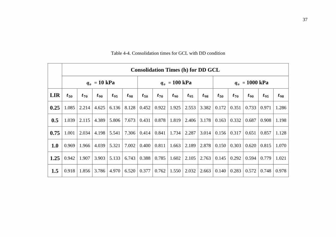
Table 4-4 shows the consolidation data for DD GCLs, and Table 4-5 presents
corresponding data for SD GCLs. As shown in Table 4-4, the longest predicted time
for 98% GCL consolidation and DD conditions is 8.128 h, which also corresponds to
low 𝑞𝑜 and low LIR. Thus, the recommended consolidation time for a GCL prior
to the start of shearing is 24 h for double-drainage. The shortest time for 98%
consolidation for DD is 0.978 h for high 𝑞𝑜 and high LIR. The minimum time in
Table 4.9 is 0.140 h, and was obtained for the 𝑡50 with 𝑞𝑜 = 1000 kPa and LIR =
1.5. For 𝑞𝑜 = 10 kPa, the range of 𝑡50 is 0.918 h ~ 1.085 h and the range of 𝑡98 is
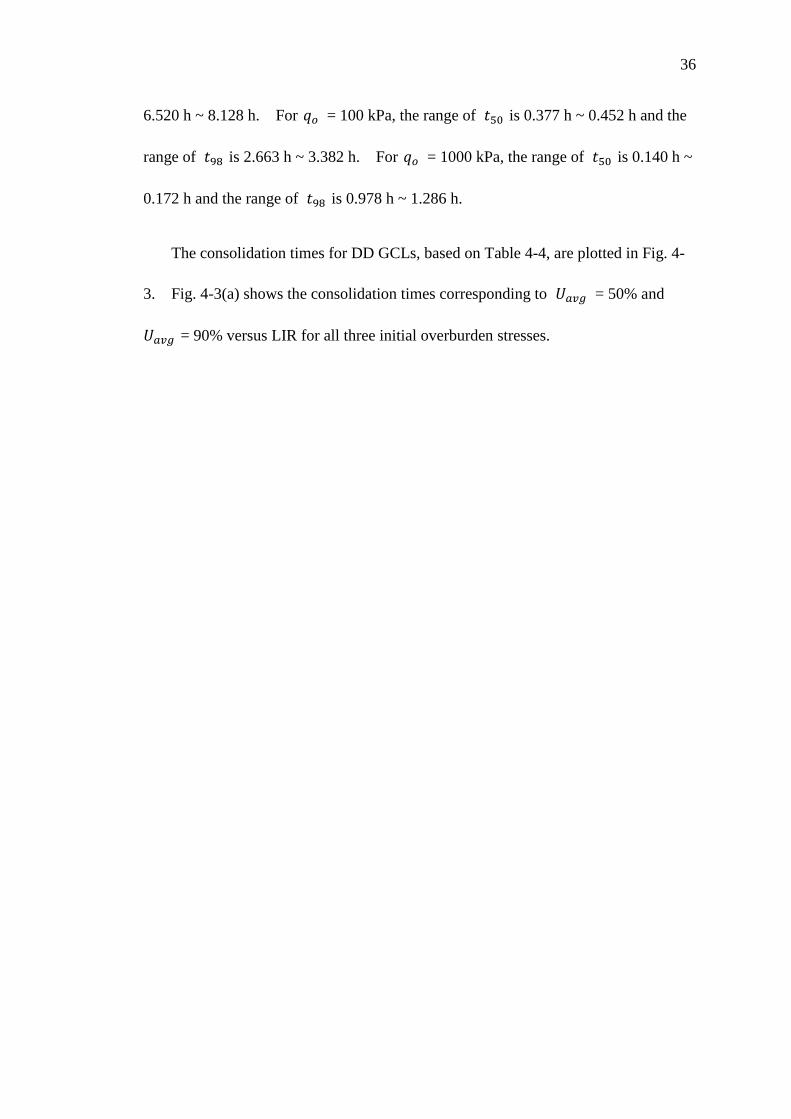
36
6.520 h ~ 8.128 h. For 𝑞𝑜 = 100 kPa, the range of 𝑡50 is 0.377 h ~ 0.452 h and the
range of 𝑡98 is 2.663 h ~ 3.382 h. For 𝑞𝑜 = 1000 kPa, the range of 𝑡50 is 0.140 h ~
0.172 h and the range of 𝑡98 is 0.978 h ~ 1.286 h.
The consolidation times for DD GCLs, based on Table 4-4, are plotted in Fig. 4-
3. Fig. 4-3(a) shows the consolidation times corresponding to 𝑈𝑎𝑣𝑔 = 50% and
𝑈𝑎𝑣𝑔 = 90% versus LIR for all three initial overburden stresses.
37
Table 4-4. Consolidation times for GCL with DD condition
Consolidation Times (h) for DD GCL
𝒒𝒐 = 10 kPa 𝒒𝒐 = 100 kPa 𝒒𝒐 = 1000 kPa
LIR 𝒕𝟓𝟎 𝒕𝟕𝟎 𝒕𝟗𝟎 𝒕𝟗𝟓 𝒕𝟗𝟖 𝒕𝟓𝟎 𝒕𝟕𝟎 𝒕𝟗𝟎 𝒕𝟗𝟓 𝒕𝟗𝟖 𝒕𝟓𝟎 𝒕𝟕𝟎 𝒕𝟗𝟎 𝒕𝟗𝟓 𝒕𝟗𝟖
0.25 1.085 2.214 4.625 6.136 8.128 0.452 0.922 1.925 2.553 3.382 0.172 0.351 0.733 0.971 1.286
0.5 1.039 2.115 4.389 5.806 7.673 0.431 0.878 1.819 2.406 3.178 0.163 0.332 0.687 0.908 1.198
0.75 1.001 2.034 4.198 5.541 7.306 0.414 0.841 1.734 2.287 3.014 0.156 0.317 0.651 0.857 1.128
1.0 0.969 1.966 4.039 5.321 7.002 0.400 0.811 1.663 2.189 2.878 0.150 0.303 0.620 0.815 1.070
1.25 0.942 1.907 3.903 5.133 6.743 0.388 0.785 1.602 2.105 2.763 0.145 0.292 0.594 0.779 1.021
1.5 0.918 1.856 3.786 4.970 6.520 0.377 0.762 1.550 2.032 2.663 0.140 0.283 0.572 0.748 0.978
38
Table 4-5. Consolidation times for GCL with SD condition
Consolidation Times (h) for SD GCL
𝒒𝒐 = 10 kPa 𝒒𝒐 = 100 kPa 𝒒𝒐 = 1000 kPa
LIR 𝒕𝟓𝟎 𝒕𝟕𝟎 𝒕𝟗𝟎 𝒕𝟗𝟓 𝒕𝟗𝟖 𝒕𝟓𝟎 𝒕𝟕𝟎 𝒕𝟗𝟎 𝒕𝟗𝟓 𝒕𝟗𝟖 𝒕𝟓𝟎 𝒕𝟕𝟎 𝒕𝟗𝟎 𝒕𝟗𝟓 𝒕𝟗𝟖
0.25 4.339 8.857 18.499 24.543 32.513 1.808 3.689 7.700 10.214 13.527 0.689 1.406 2.931 3.886 5.145
0.5 4.155 8.459 17.556 23.226 30.691 1.725 3.510 7.277 9.624 12.711 0.654 1.329 2.749 3.632 4.793
0.75 4.005 8.135 16.793 22.165 29.225 1.658 3.365 6.936 9.149 12.055 0.624 1.266 2.602 3.428 4.512
1.0 3.877 7.863 16.157 21.283 28.008 1.601 3.243 6.652 8.754 11.512 0.600 1.214 2.481 3.259 4.279
1.25 3.768 7.629 15.614 20.531 26.974 1.552 3.139 6.410 8.419 11.051 0.579 1.169 2.377 3.116 4.083
1.5 3.672 7.426 15.143 19.880 26.080 1.509 3.048 6.200 8.129 10.653 0.560 1.130 2.287 2.993 3.913

39
0
1
2
3
4
5
0.25 0.5 0.75 1 1.25 1.5
qo = 10 kPa
qo = 100 kPa
qo = 1000 kPa
Load Increment Ratio, LIR
Open symbol: t50
Solid symbol: t90
(a)t 5
0 a
nd
t90 (
h)
0
2
4
6
8
10
0.25 0.5 0.75 1 1.25 1.5
qo = 10 kPa
qo = 100 kPa
qo = 1000 kPa
t 95 a
nd
t9
8 (
h)
Load Increment Ratio, LIR
Open symbol: t95
Solid symbol: t98
(b)
Figure 4-3. Consolidation data for DD GCLs: (a) 𝑡50 and 𝑡90; (b) 𝑡95 and 𝑡98
40
As indicated in Fig. 4-3, under the same conditions (i.e. same 𝑞𝑜 and at the same
degree of consolidation), the consolidation time decreases as LIR increases. For
example, when the initial overburden stress is 10 kPa and the load increment ratio is
0.25, 1.085 h is required to reach 𝑈𝑎𝑣𝑔 = 50%; when the LIR is 0.5, 𝑡50 is 1.039 h,
which is less than that of LIR = 0.25; when the LIR is 0.75, 𝑡50 is 1.001 h, and that is
even less than that of LIR = 0.5.
Additionally, the GCLs under greater initial effective overburden stress also
consolidate faster as shown in Fig. 4-3. Corresponding to the same LIR and degree
of consolidation, the GCLs under 𝑞𝑜 = 10 kPa require more time for consolidation
than that under 𝑞𝑜 = 100 kPa, and the GCLs under 𝑞𝑜 = 100 kPa take more time than
GCLs under 𝑞𝑜 = 1000 kPa.
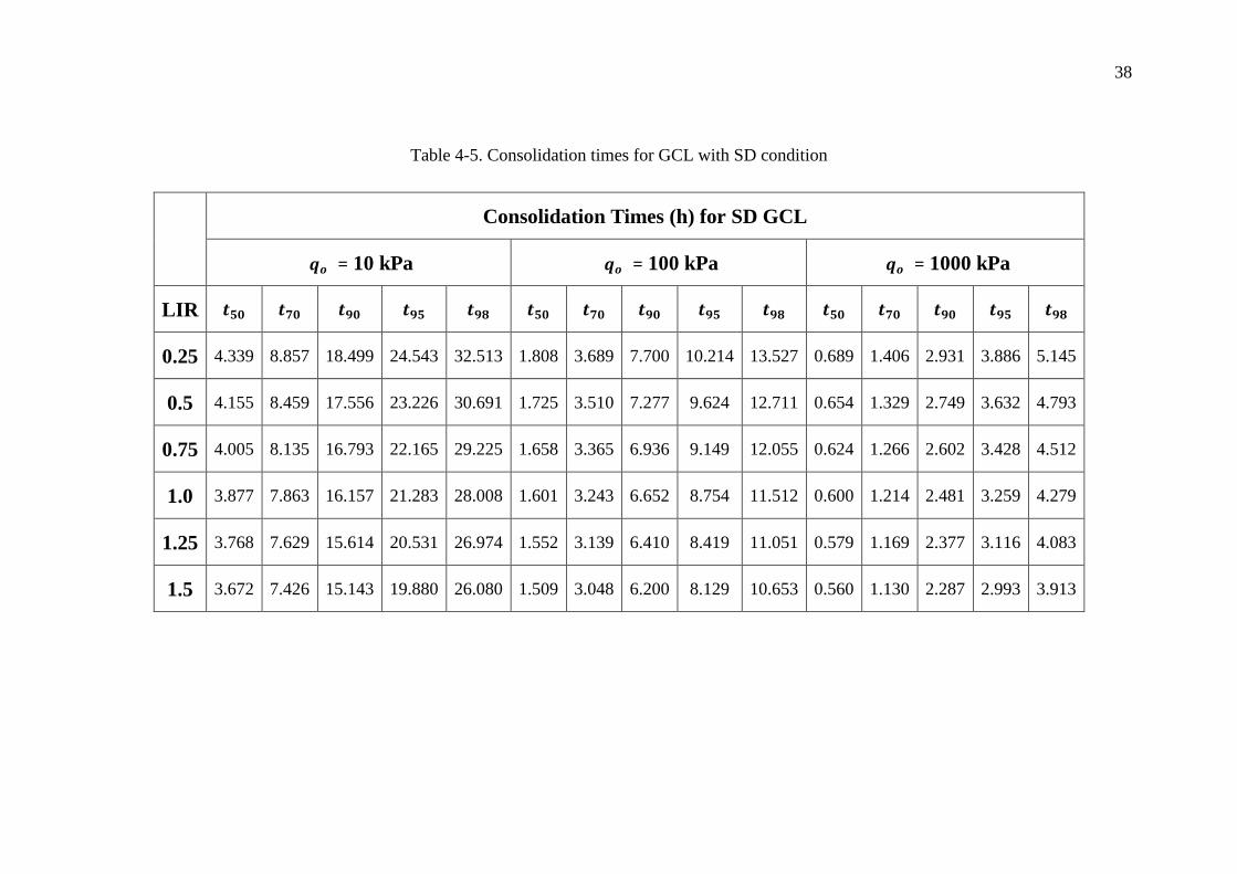
As shown in Table 4-5, the longest predicted time required for 98% GCL
consolidation and SD conditions is 32.513 h, which corresponds to low initial
overburden stress and low LIR. Thus, for a direct shear test, the recommended
consolidation time for a GCL prior to the start of shearing is 48 h for single-drainage.
The minimum time is 0.560 h, and occurs for 𝑡50 with 𝑞𝑜 = 1000 kPa and LIR =
1.5. For 𝑞𝑜 = 10 kPa and all six load increments, the range of 𝑡50 is 3.672 h ~
4.339 h and the range of 𝑡98 is 26.080 h ~ 32.513 h. For 𝑞𝑜 = 100 kPa, the range of
𝑡50 is 1.509 h ~ 1.808 h and the range of 𝑡98 is 10.653 h ~ 13.527 h. For 𝑞𝑜 = 1000
kPa, the range of 𝑡50 is 0.560 h ~ 0.689 h and the range of 𝑡98 is 3.913 h ~ 5.145 h.

41
The consolidation times for SD GCLs, based on the Table 4-5, are plotted in Fig.
4-4. Fig. 4-4(a) shows the consolidation times corresponding to 𝑈𝑎𝑣𝑔 = 50% and
𝑈𝑎𝑣𝑔 = 90% versus LIR under all three initial overburden stresses.
The regular patterns regarding consolidation times observed in DD GCLs are also
applicable to those of SD GCLs: under the same circumstances (i.e. the same GCL
under the same initial overburden stress and at the same degree of consolidation), the
consolidation times decrease as LIR increases; additionally, the GCLs under greater
initial overburden stress also consolidate faster as shown in Fig. 4-4. These two
patterns are described in more detail below.
First, SD GCLs subjected to greater LIR require less time to reach the same
degree of consolidation under the same conditions. For instance, when the initial
overburden stress is 10 kPa and the load increment ratio is 0.25, 4.339 h are required
to reach 𝑈𝑎𝑣𝑔 = 50%; when the LIR is 0.5, 𝑡50 is 4.155 h, which is a little less than
that of LIR = 0.25; however, when the LIR is 0.75, 𝑡50 is 4.005 h, and that is less
than that of LIR = 0.5.
Second, SD GCLs under greater initial overburden stress also consolidate faster
as shown in Fig. 4-4. Corresponding to the same LIR and degree of consolidation,
the GCLs under 𝑞𝑜 = 10 kPa always require more time for consolidation than that
under 𝑞𝑜 = 100 kPa, and the GCLs under 𝑞𝑜 = 100 kPa always require more time
than GCLs under 𝑞𝑜 = 1000 kPa.

42
0
5
10
15
20
0.25 0.5 0.75 1 1.25 1.5
qo = 10 kPa
qo = 100 kPa
qo = 1000 kPa
Load Increment Ratio, LIR
Open symbol: t50
Solid symbol: t90
(a)
t 50 a
nd
t9
0 (
h)
0
5
10
15
20
25
30
35
0.25 0.5 0.75 1 1.25 1.5
qo = 10 kPa
qo = 100 kPa
qo = 1000 kPa
t 95 a
nd
t9
8 (
h)
Load Increment Ratio, LIR
Open symbol: t95
Solid symbol: t98
(b)
Figure 4-4.Consolidation data for SD GCLs: (a) 𝑡50 and 𝑡90; (b) 𝑡95 and 𝑡98

43
The time for consolidation depends on the relative effect of compressibility
relationship versus hydraulic conductivity relationship. Compressibility relationship
decides ultimate settlement under certain effective stress, and hydraulic conductivity
relationship decides the reduction in hydraulic conductivity which essentially affects
the relative flow velocity. The consolidation times decrease as LIR increases. In
this case, higher LIR gives relatively less reduction in hydraulic conductivity, and the
effect of hydraulic conductivity plays a more important role. Thus, consolidation
under higher LIR is faster than that for low LIR.
4.4 Ratio of Consolidation Times for DD and SD Conditions
Terzaghi’s consolidation theory indicates that the consolidation time for the SD
condition should be four times greater than for the DD condition due to the effect of
drainage distance. In the current study, ratios of the consolidation times for SD
GCLs and DD GCLs from CS2 are compared with Terzaghi theory.
The ratio of consolidation time between SD and DD GCLs is summarized in
Table 4-6. Table 4-6 has an identical configuration with Table 4-4 and Table 4-5,
and presents the data of ratio of consolidation times for SD and DD conditions.
Most of the values essentially equal 4.0 and the differences can only be noticed after 3
or 4 decimal places. Thus, Table 4-6 chooses to use 6 decimal points in order to
present these differences.
The consolidation time ratios for DD and SD GCLs, based on the Table 4-6, are
plotted in Fig. 4-5. Fig. 4-5(a) shows the consolidation time ratios corresponding to

44
𝑈𝑎𝑣𝑔 = 50% and 𝑈𝑎𝑣𝑔 = 90% versus LIR under all three initial overburden stresses.
Likewise, Fig. 4-5(b) shows the consolidation time ratios corresponding to 𝑈𝑎𝑣𝑔 =
95% and 𝑈𝑎𝑣𝑔 = 98%.

45
Table 4-6. Ratios of consolidation times of SD GCLs to DD GCLs
Time ratios for SD GCLs/DD GCLs
𝒒𝒐 = 10 kPa 𝒒𝒐 = 100 kPa 𝒒𝒐 = 1000 kPa
LIR 𝒕𝟓𝟎 𝒕𝟕𝟎 𝒕𝟗𝟎 𝒕𝟗𝟓 𝒕𝟗𝟖 𝒕𝟓𝟎 𝒕𝟕𝟎 𝒕𝟗𝟎 𝒕𝟗𝟓 𝒕𝟗𝟖 𝒕𝟓𝟎 𝒕𝟕𝟎 𝒕𝟗𝟎 𝒕𝟗𝟓 𝒕𝟗𝟖
0.25 4.0000
68
4.0000
70
4.0000
77
4.0000
77
4.0000
74
4.0000
63
4.0000
67
4.0000
75
4.0000
75
4.0000
73
4.0000
54
4.0000
62
4.0000
72
4.0000
73
4.0000
72
0.5 4.0001
42
4.0001
07
4.0000
95
4.0000
90
4.0000
84
4.0001
33
4.0001
02
4.0000
92
4.0000
88
4.0000
83
4.0001
17
4.0000
92
4.0000
87
4.0000
84
4.0000
80
0.75 4.0002
01
4.0001
36
4.0001
09
4.0001
01
4.0000
93
4.0001
90
4.0001
29
4.0001
05
4.0000
98
4.0000
91
4.0001
68
4.0001
17
4.0000
98
4.0000
93
4.0000
86
1 4.0002
50
4.0001
60
4.0001
21
4.0001
10
4.0001
00
4.0002
37
4.0001
52
4.0001
16
4.0001
07
4.0000
97
4.0002
11
4.0001
37
4.0001
08
4.0001
00
4.0000
92
1.25 4.0002
91
4.0001
80
4.0001
31
4.0001
18
4.0001
06
4.0002
76
4.0001
72
4.0001
26
4.0001
14
4.0001
03
4.0002
47
4.0001
55
4.0001
16
4.0001
06
4.0000
97
1.5 4.0003
26
4.0001
98
4.0001
39
4.0001
24
4.0001
11
4.0003
10
4.0001
88
4.0001
34
4.0001
20
4.0001
08
4.0002
78
4.0001
70
4.0001
24
4.0001
12
4.0001
01

46
4.00005
4.0001
4.00015
4.0002
4.00025
4.0003
4.00035
0.25 0.5 0.75 1 1.25 1.5
qo = 10 kPa
qo = 100 kPa
qo = 1000 kPa
Load Increment Ratio, LIR
Open symbol: t50
Solid symbol: t90
(a)T
ime R
ati
os
of
SD
to
DD
4.00007
4.00008
4.00009
4.0001
4.00011
4.00012
4.00013
0.25 0.5 0.75 1 1.25 1.5
qo = 10 kPa
qo = 100 kPa
qo = 1000 kPa
Tim
e R
ati
os
of
SD
to
DD
Load Increment Ratio, LIR
Open symbol: t95
Solid symbol: t98
(b)
Figure 4-5. Time ratios of SD to DD versus LIR: (a) 𝑡50 and 𝑡90; (b) 𝑡95 and 𝑡98

47
The values indicate that, for the conditions of this study, GCL consolidation
conforms closely to Terzaghi’s consolidation theory. Interestingly, some
phenomenon can be also observed. First, these ratios are fractionally greater than 4.
Second, for the same initial overburden stress and degree of consolidation, the ratios
increase as the LIR increases.
4.5 Comparison of Solutions for 𝑮𝒔 = 1 and 𝑮𝒔 = 2.21
Because GCLs are thin materials, the self-weight of GCLs are small, and thus, a
specific gravity of 1.0 was used for most of the CS2 simulations. However, six
additional simulations were conducted with the equivalent 𝐺𝑠 = 2.21 for comparison.
The results with 𝐺𝑠 = 2.21 are summarized in Table 4-7. As shown in Table 4-
7, the data for 𝐺𝑠 = 2.21 is nearly identical to the data form 𝐺𝑠 = 1, with agreement
to the first three decimal places for most cases. The largest error between the values
from 𝐺𝑠 = 2.21 and that from 𝐺𝑠 = 1 is less than 0.1%. This comparison indicates
that the effect of self-weight of GCL solids is negligible, because GCLs are thin
materials.

48
Table 4-7. Comparison of simulation results for 𝐺𝑠 = 2.21 and 𝐺𝑠 = 1
Consolidation Times (h) for 𝑮𝒔 = 2.21 Consolidation Times (h) for 𝑮𝒔 = 1
𝒕𝟓𝟎 𝒕𝟕𝟎 𝒕𝟗𝟎 𝒕𝟗𝟓 𝒕𝟗𝟖 𝒕𝟓𝟎 𝒕𝟕𝟎 𝒕𝟗𝟎 𝒕𝟗𝟓 𝒕𝟗𝟖
DD
𝒒𝒐 = 10 kPa,
LIR = 0.5
1.03868
9
2.11448
4
4.38846
3
5.80610
0
7.67206
6
1.03877
8
2.11465
6
4.38877
5
5.80648
7
7.67254
7
𝒒𝒐 = 100 kPa,
LIR = 1
0.40013
4
0.81081
5
1.66289
8
2.18855
3
2.87784
9
0.40013
4
0.81081
6
1.66289
8
2.18855
1
2.87784
4
𝒒𝒐 = 1000 kPa,
LIR = 1.5
0.14008
0
0.28250
7
0.57181
8
0.74811
1
0.97826
1
0.14008
0
0.28250
7
0.57181
8
0.74811
0
0.97826
0
SD
𝒒𝒐 = 10 kPa,
LIR = 0.5
4.15789
4
8.46308
5
17.5629
19
23.2358
33
30.7027
72
4.15525
9
8.45884
9
17.5555
16
23.2264
71
30.6908
34
𝒒𝒐 = 100 kPa,
LIR = 1
1.60072
7
3.24354
1
6.65204
9
8.75477
0
11.5120
80
1.60063
2
3.24338
8
6.65178
5
8.75443
7
11.5116
57
𝒒𝒐 = 1000 kPa,
LIR = 1.5
0.56036
3
1.13008
2
2.28735
1
2.99253
8
3.91315
5
0.56036
0
1.13007
7
2.28734
1
2.99252
5
3.91314
0
SD/DD
Ratio
𝒒𝒐 = 10 kPa,
LIR = 0.5
4.00302
0
4.00243
4
4.00206
6
4.00196
9
4.00189
1
4.00014
2
4.00010
7
4.00009
5
4.00009
0
4.00008
4
𝒒𝒐 = 100 kPa,
LIR = 1
4.00048
1
4.00034
5
4.00027
4
4.00025
5
4.00023
8
4.00023
7
4.00015
2
4.00011
6
4.00010
7
4.00009
7
𝒒𝒐 = 1000 kPa,
LIR = 1.5
4.00029
9
4.00018
6
4.00013
7
4.00012
4
4.00011
3
4.00027
8
4.00017
0
4.00012
4
4.00011
2
4.00010
1
49
Chapter 5
Conclusions and Future Research
5.1 Conclusions
This thesis presents a numerical investigation of the consolidation behavior for
GCLs and estimates consolidation times of shear strength testing for GCLs. Using
the numerical model CS2 (Fox and Berles 1997; Fox and Hefu 2012), variable
conditions for GCL consolidation are assessed, such as three initial overburden
stresses, six load increment ratios, DD and SD drainage conditions, and two specific
gravities. These simulations have led to the following conclusions:
1. The longest predicted time required for 98% GCL consolidation and SD
conditions is 32.5 h, which corresponds to low initial effective stress and low
LIR. Thus, for a direct shear test, the recommended consolidation time for a
GCL prior to the start of shearing is 48 h for single-drainage conditions.
2. The longest predicted time required for 98% GCL consolidation and DD
conditions is 8.1 h, which also corresponds to low initial effective stress and low
LIR. Thus, the recommended consolidation time for a GCL prior to the start of
shearing is 24 h or overnight for double-drainage conditions.
3. For both DD and SD GCLs, under the same initial overburden effective stress, the
time needed to reach the same degree of consolidation decreases as the load
increment ratio increases. Thus, greater load increments could reduce GCL

50
consolidation times; however, bentonite extrusion may become problematic with
increasing load increment. For any given load increment ratio, GCLs under
greater initial overburden stress consolidate faster regardless of drainage
conditions.
4. CS2 solutions indicate that the ratio of consolidation time for DD to SD
conditions is approximately equal to 4.0 in all cases, which is consistent with
classical consolidation theory.
5. The numerical solutions obtained for 𝐺𝑠 = 1 are essentially the same as the
corresponding solutions for 𝐺𝑠 = 2.21. The comparison between the
simulations of 𝐺𝑠 = 1 and 𝐺𝑠 = 2.21 indicates that the effect of self-weight of
GCL solids is negligible, and this occurs because GCLs are thin materials.
5.2 Future Research
In general, shear strengths for GCLs and GCL interfaces are a function of the
effective normal stress on the failure surface. In the field, GCLs are typically
drained and excess pore pressure is assumed to be very small for static stability
analysis. This is because (except encapsulated GCLs): firstly, GCLs are thin
materials and mostly drained at least on one side; secondly, the rates of loading in the
field are relatively slow, compared with the rate of GCL consolidation (Gilbert et al.
1997).
Laboratory tests use total normal stress on the failure plane to express the strength
of GCLs and GCL interfaces, and the shear-induced pore pressure, in this case, is
crucial. Due to the difficulty to measure the pore pressures on the failure plane,

51
whether shear-induced excess pore pressures occur on the failure surface is unknown
(Fox et al. 1998, Eid et al. 1999). Fox et al. (1998) suggests that the excess pore
pressure is negligible at the failure surface of woven geotextile-supported GCLs; Eid
et al. (1999) suggests that woven geotextile-supported GCLs might develop excess
pore pressure because the migration of bentonite into such GCLs could reduce
hydraulic conductivity. Based on volume change and shear strength data over a
wide range of normal stress levels and displacement rates, that was concluded that
excess pore pressure on failure surface increased as the increase of the normal stress
and displacement rate (Fox et al. 2015; Ross and Fox 2015).
GCL shear strength is a function of effective normal stress, but is generally
expressed in terms of total normal stress in laboratory direct shear tests because pore
pressures are difficult to measure. Thus, it would be an interesting topic to
investigate the effect of shear-induced excess pore pressure on the GCL shear strength
using numerical modeling. The main work is to develop relationships among
volume change, displacement rate, normal stress, and shear strength. Using the
methods of this thesis, a new model incorporating the relationships can be developed
to predict acceptable shear displacement rates for direct shear tests.
.

52
References
Al-Tabbaa, A., and Wood, D. M. (1987). Some measurements of the permeability of
kaolin. Geotechnique, 37(4), 499-503.
ASTM D2487, Standard Practice for Classification of Soils for Engineering Purposes
(Unified Soil Classification System), ASTM International, West
Conshohocken, PA, 2011, www.astm.org
ASTM D4318, Standard Test Methods for Liquid Limit, Plastic Limit, and Plasticity
Index of Soils, ASTM International, West Conshohocken, PA,
2010, www.astm.org
ASTM D6243, Standard Test Method for Determining the Internal and Interface
Shear Strength of Geosynthetic Clay Liner by the Direct Shear Method, ASTM
International, West Conshohocken, PA, 2016, www.astm.org
Castelbaum, D., and Shackelford, C. D. (2009). Hydraulic conductivity of bentonite
slurry mixed sands. Journal of Geotechnical and Geoenvironmental
Engineering, 135(12), 1941-1956.
Daniel, D. E., Shan, H.-Y. and Anderson, J. D. (1993). Effects of partial wetting on
the performance of the bentonite component of a geosynthetic clay liner.
Proceedings of Geosynthetics ‘93, Vancouver, Canada, Industrial Fabrics
Association International, Roseville, MI, USA, Vol. 3, pp. 1483–1496.
Eid, H., and Stark, T. (1997). Shear Behavior of an Unreinforced Geosynthetic Clay
Liner. Geosynthetics International, 4(6), 645-659. doi:10.1680/gein.4.0109

53
Eid, H. T., Stark, T. D. and Doerfler, C. K. (1999). Effect of shear displacement rate
on internal shear strength of a reinforced geosynthetic clay liner. Geosynthetics
International, 6(3), 219–239.
Fox, P. J. (1999). Solution charts for finite strain consolidation of normally
consolidated clays. Journal of Geotechnical and Geoenvironmental
Engineering, 125(10), 847-867.
Fox, P. J. (2000). “CS4: A large strain consolidation model for accreting soil layers.”
Geotechnics of High Water Content Materials, Special Technical Publication
1374, T. B. Edil and P. J. Fox, eds., ASTM, West Conshohocken, PA, 29–47.
Fox, P. J. (2007a). “Coupled large strain consolidation and solute transport. I—Model
development.” Journal of Geotechnical and Geoenvironmental Engineering,
133(1), 3–15.
Fox, P. J. (2007b). “Coupled large strain consolidation and solute transport. II—
Model verification and simulation results.” Journal of Geotechnical and
Geoenvironmental Engineering, 133(1), 16–29.
Fox, P. J., and Berles, J. D. (1997). CS2: A PIECEWISE‐LINEAR MODEL FOR
LARGE STRAIN CONSOLIDATION. International Journal for Numerical
and Analytical Methods in Geomechanics, 21(7), 453-475.
Fox, P. J., and Qiu, T. (2004). “Model for large strain consolidation with compressible
pore fluid.” International Journal for Numerical and Analytical Methods in
Geomechanics, 28(11), 1167–1188.

54
Fox, P. J., Lee, J., and Qiu, T. (2005). “Model for large strain consolidation by
centrifuge.” International Journal of Geomechanics, 5(4), 267–275.
Fox, P. J., and Lee, J. (2008). “Model for consolidation-induced solute transport with
nonlinear and nonequilibrium sorption.” International Journal of
Geomechanics, 8(3), 188–198.
Fox, P. J., and Pu, H. (2012). Enhanced CS2 model for large strain
consolidation. International Journal of Geomechanics, 12(5), 574-583.
Fox, P. J., and Stark, T. D. (2015). State-of-the-art report: GCL shear strength and its
measurement—Ten-year update. Geosynthetics International, 22(1), 3-47.
Fox, P. J., Rowland, M. G., Scheithe, J. R., Davis, K. L., Supple, M. R., and Crow, C.
C. (1997). Design and evaluation of a large direct shear machine for
geosynthetic clay liners. Geotechnical Testing Journal, 20, 279-288.
Fox, P. J., Rowland, M. G., and Scheithe, J. R. (1998). Internal shear strength of three
geosynthetic clay liners. Journal of Geotechnical and Geoenvironmental
Engineering, 124(10), 933–944.
Fox, P. J., Di Nicola, M., and Quigley, D. W. (2003). “Piecewise-linear model for
large strain radial consolidation.” Journal of Geotechnical and
Geoenvironmental Engineering, 129(10), 940–950.
Fox, P. J., Stark, T. D., and Swan, R. H. (2004, January). Laboratory measurement of
GCL shear strength. In Advances in Geosynthetic Clay Liner Technology: 2nd
Symposium. ASTM International.

55
Fox, P. J., Nye, C. J., Morrison, T. C., Hunter, J. G., and Olsta, J. T. (2006). Large
dynamic direct shear machine for geosynthetic clay liners. ASTM geotechnical
testing journal, 29(5), 392-400.
Fox, P. J., Pu, H. F., and Berles, J. D. (2014). CS3: Large strain consolidation model
for layered soils. Journal of Geotechnical and Geoenvironmental
Engineering, 140(8), 04014041.
Fox, P. J., Sura, J. M., and Nye, C. J. (2015). Dynamic Shear Strength of a Needle-
Punched GCL for Monotonic Loading. Journal of Geotechnical and
Geoenvironmental Engineering, 141(7), 04015025.
GCL products. [Photograph]. From
http://img.bhs4.com/29/7/297B2927C78EC0BC4D8D9B37F539AD59A28C8
7A4_large.jpg
GCL installation on side slope of a bottom liner system. [Photograph]. From
http://www.exportersindia.com/gorantlageosyntheticspvtltd/products.htm#geo
synthetic-clay-liner-chennai-india-1384768
Gilbert, R. B., Scranton, H. B. and Daniel, D. E. (1997). Shear strength testing for
geosynthetic clay liners. Testing and Acceptance Criteria for Geosynthetic
Clay Liners, Well, L. W., Editor, ASTM International, West Conshohocken,
PA, USA, pp. 121–135, STP 1308.
Hewitt, R. D., Soydemir, C., Stulgis, R. P. and Coombs, M. T. (1997). Effect of

56
normal stress during hydration and shear on the shear strength of GCL/textured
geomembrane interfaces. Testing and Acceptance Criteria for Geosynthetic
Clay Liners, Well, L. W., Editor, ASTM International, West Conshohocken,
PA, USA, pp. 55–70, STP 1308.
Kang, J. B., and Shackelford, C. D. (2010). Consolidation of a geosynthetic clay liner
under isotropic states of stress. Journal of Geotechnical and Geoenvironmental
Engineering, 136(1), 253-259.
Lake, C., & Rowe, R. (2000). Diffusion of sodium and chloride through geosynthetic
clay liners. Geotextiles and Geomembranes, 18(2-4), 103-131.
doi:10.1016/s0266-1144(99)00023-0
Lee, J., and Fox, P. J. (2009). “Investigation of consolidation-induced solute transport.
II: Experimental and numerical results.” Journal of Geotechnical and
Geoenvironmental Engineering, 135(9), 1239–1253.
Marr, W. A. (2001). “Interface and Internal Shear Testing Procedures to Obtain Peak
and Residual Values.” 15th GRI Conference: Hot Topics in Geosynthetics
(Peak/Residual; RECMs; Installation; Concerns). Houston, TX, pp. 1-27.
Malusis, M. A., and Shackelford, C. D. (2002). Chemico-osmotic efficiency of a
geosynthetic clay liner. Journal of Geotechnical and Geoenvironmental
Engineering, 128(2), 97-106.
McCartney, J. S., Zornberg, J. G. and Swan, R. H. Jr. (2009). Analysis of a large
database of GCL-geomembrane interface shear strength results. Journal of
Geotechnical and Geoenvironmental Engineering, 135(2), 209–223.

57
Nagaraj, T. S., Pandian, N. S., and Narasimha Raju, P. S. R. (1994). “Stressstate-
permeability relations for overconsolidated clays.”Geotechnique, 44(2), 349–
352.
Olson, R. E. (1977). “Consolidation under time-dependent loading.” Journal of the
Geotechnical Engineering Division, 103(1), 55–60.
Ross, J. D., and Fox, P. J. (2015). Dynamic Shear Strength of GMX/GCL Composite
Liner for Monotonic Loading. Journal of Geotechnical and Geoenvironmental
Engineering, 141(7), 04015026. doi:10.1061/(asce)gt.1943-5606.0001198
Trauger, R. and Darlington, J. (2000). Next-generation geosynthetic clay liners for
improved durability and performance. TR-220, Colloid Environmental
Technologies Company, Arlington Heights, IL, USA, pp. 2–14.
Triplett, E. J. and Fox, P. J. (2001). Shear strength of HDPE
geomembrane/geosynthetic clay liner interfaces. Journal of Geotechnical and
Geoenvironmental Engineering, 127(6), 543–552.
Vukelic, A., Szavits-Nossan, A. and Kvasnicka, P. (2008). The influence of bentonite
extrusion on shear strength of GCL/geomembrane interface. Geotextiles and
Geomembranes, 26(1), 82–90.
Zelic, B. K., Znidarcic, D. and Kovacic, D. (2002). Shear strength testing on a GCL.
Proceedings of 7th International Conference on Geosynthetics, Nice, France,
Vol. 4, pp. 1329–1334.
Zornberg, J. G., McCartney, J. S. and Swan, R. H. Jr. (2006). Closure to ‘Analysis of
a large database of GCL internal shear strength results’ by Zornberg, J. G.,
58
McCartney, J. S. and Swan, R, H. Jr. Journal of Geotechnical and
Geoenvironmental Engineering, 132(10), 1376–1379.

59
Appendices
Notation
The following symbols are used in this thesis:
𝑎𝑣 = coefficient of compressibility;
𝐶𝑐 = compression index;
𝐶𝑟 = recompression index;
𝐶𝑘 = coefficient of hydraulic conductivity;
𝑐𝑣 = coefficient of consolidation;
𝑒 = void ratio;
𝑒𝑓 = final void ratio;
𝑒0 = initial void ratio;
𝑒𝑝 = preconsolidation void ratio;
𝑓𝑜 = initial seepage force per unit volume;
𝐺𝑠 = specific gravity of solids;
𝐻 = height of soil layer;
𝐻𝑑𝑟 = longest drainage path;
𝐻𝑜 = initial height of soil layer;
ℎ = total head;
ℎ𝑏 = total head at bottom boundary;
ℎ𝑡 = total head at top boundary;
𝑖 = hydraulic gradient;
𝑗 = element coordinate;

60
𝑘 = vertical hydraulic conductivity;
𝑘𝑜 = initial vertical hydraulic conductivity;
𝑘𝑠 = equivalent series vertical hydraulic conductivity;
𝐿 = height of element;
𝐿𝑜 = initial height of element;
𝑞𝑜 = initial vertical effective stress at top boundary;
𝑅𝑗 = number of elements;
𝑅𝑠 = number of data points for compressibility relationship;
𝑅𝑡 = number of data points for hydraulic conductivity relationship;
𝑆 = settlement of soil layer;
𝑆𝑢𝑙𝑡 = ultimate settlement of soil layer;
𝑇 = time factor;
𝑡 = time;
𝑈𝑎𝑣𝑔 = average degree of consolidation;
𝑢 = pore pressure;
𝑢𝑒𝑥 = excess pore pressure;
𝑣𝑟𝑓 = relative discharge velocity;
𝑣𝑜 = steady discharge velocity;
𝑧 = vertical coordinate;
𝑧𝑜 = initial elevation of element node;
𝛼 = constant;
𝛾 = saturated unit weight of soil;

61
𝛾𝑜′ = initial buoyant unit weight of soil;
𝛾𝑤 = unit weight of water;
∆𝑞 = change in vertical effective stress at top boundary;
∆𝑞𝑚𝑎𝑥 = maximum vertical effective stress at top boundary;
∆𝑡 = time increment;
𝜎 = vertical total stress;
𝜎′ = vertical effective stress;
𝜎𝑜′ = initial vertical effective stress; and
𝜎𝑝′ = preconsolidation stress.
Superscripts
𝑡 = time;
^ = data points for compressibility relationship;
– = data points for hydraulic conductivity relationship; and
∼ = data points for loading schedule.
Subscripts
𝑏 = summation index;
𝑗 = 𝑗𝑡ℎ element;
𝑅𝑗 = top element;
𝑠 = 𝑠𝑡ℎ data point for compressibility relationship; and
𝑡 = 𝑡𝑡ℎ data point for hydraulic conductivity relationship.