Prediction of extreme geophysical, industrial and biophysical

Prediction of extreme geophysical, industrial and

biophysical flows using particle methods

P.W. Cleary a, R.C.Z. Cohen

a, S. Harrison

a, M. Sinnott

a, M. Prakash

a and S. Mead

a

a Mathematics, Informatics and Statistics, CSIRO, Clayton, Victoria

Email: [email protected]

Abstract: The flow of particulates and fluids is critical to many applications. Examples include human

processes such as eating and locomotion, extreme geophysical flows such as tsunamis and dam-collapse

inundation, biomedical applications such as transport of material in the gastro-intestinal tract and heart assist

pumps, and industrial processes such as crushing and grinding (comminution).

Meshless particle based methods such DEM (Discrete Element Method) and SPH (Smoothed Particle

Hydrodynamics) have a range of strong advantages over traditional grid based continuum methods for these

types of applications. The advantages include:

the ability to include particle level information in collision dominated particle flows

ability to resolve complex fluid free surfaces including splashing and fragmentation

ability to predict very large deformations, including fracture

interaction with moving and deforming solid bodies or objects

ability to track material history and use this in the flow modelling such as the rheology.

These advantages are demonstrated in a series of computationally demanding examples and case studies

including crushers and mills, biomedical pumps and transport of faecal matter in the bowel, geophysical

extreme flow events (risk/disaster modelling), eating of food by humans and elite water based sports.

In all cases, there are significant sources of variability that need to be taken into account in the modelling:

For human based models the major sources of variability are the nature of the motions of the human

(both internal and external). Such variations can be short term (cycle variation between repetitions),

medium term such as changes in response to fatigue or the relative timing and strengths of

repetitions over time or longer term (such as in response to injury or deliberate planned changes).

For the geophysical/disaster modelling, variability is mainly reflected in the range and nature of the

scenarios that need to be considered in building risk frameworks in which these models can predict

specific consequences. For examples, the range of possible failure scenarios of a dam or the range of

heights, speeds and water volumes for tsunamis generated by poorly understood initiation events.

Finally, in all such applications there is uncertainty about material properties and the details of the

initial conditions whose effects need to be understood. For example, in comminution (either in an

industrial crusher or mill or in the human mouth during chewing) the performance of the process is

heavily influenced by the specific nature of the material being comminuted. This can vary strongly

between materials and between different instances of what is nominally the same material. In the

human eating case, this is further complicated by feedback from the material nature into the detailed

nature of the chewing motion.

Such variability influences both the inputs to specific instances of the deterministic models and the usage

scenarios that need to be considered to understand the range of behaviours that exist for these processes.

Optimisation and decision making based on such models cannot be reasonably performed without

considering these issues. The ultimate usefulness of the model outcomes is heavily dependent on the quality

of the management of these uncertainties.

Keywords: Smoothed particle hydrodynamics (SPH), discrete element method (DEM), geophysical flows,

industrial flows, biophysical flows

19th International Congress on Modelling and Simulation, Perth, Australia, 12–16 December 2011 http://mssanz.org.au/modsim2011

1

Cleary et al., Prediction of extreme geophysical, industrial and biophysical flows using particle methods

1. INTRODUCTION

DEM has been developed and used over the last 30 years for modelling flows of particulate solids in many

applications, starting with small systems in simple geometries in two-dimensions (Cundall and Strack, 1979;

Walton, 1994; Campbell, 1990; Haff and Werner, 1986). It is now possible to simulate systems of tens of

millions of particles on desktop computers (Cleary, 2004, 2009) enabling many complex particulate flows to

be predicted. It is the most effective method for modelling flow controlled by collisions of particulates.

SPH is a powerful particle method well suitable for solving complex multi-physics flow and deformation

problems. It is particularly well suited to splashing free surface flows, interaction with dynamic moving

bodies and discrete particles. It also has strong advantages in situations where flow or material history is

important. The method was first developed for use with incompressible fluid flows by Monaghan (1994).

Many examples of the application of SPH are given in Cleary et al. (2007).

The inherent flexibility of these two Lagrangian techniques allows them to be easily and effectively applied

to a wide range of different modelling problems. An important issue for such modelling is the inherent

uncertainties that surround it. Whilst each simulation is deterministic in nature, there are often uncertainties

in model inputs and in the range of scenarios that can occur with each flow. In this paper we describe a sub-

set of the applications where such numerical methods have been applied and highlight the diversity of

physics and modelling scenarios that can be readily handled by DEM and SPH and how uncertainty

influences such modelling.

2. PARTICLE METHODS

DEM is a simulation method that models particulate systems whose motions are dominated by collisions.

This involves following the motion of every particle or object in the flow and modelling each collision

between the particles and between the particles and their environment. The algorithm has three main stages:

1. A search grid is used to periodically build a near-neighbour interaction list that contains all the particle

pairs and object-particle pairs that are likely to experience collisions in the short term.

2. The forces on each pair of colliding particles and/or boundary objects are evaluated in their local

reference frame using a suitable contact force model, and then transformed into the simulation.

3. All the forces and torques on each particle and object are summed and the resulting equations of motion

are integrated to give the resulting motion of these bodies.

The implementation used here is described in more detail in Cleary (2004, 2009). The entities are allowed to

overlap and the amount of overlap x, and normal vn and tangential vt relative velocities determine the

collisional forces via a contact force law. We use a linear spring-dashpot model where the normal and

tangential forces are given by:

nnnn vCxkF , ttttnt vCdtvkFF ,min (1)

The normal force consists of a linear spring to provide the repulsive force and a dashpot to dissipate a

proportion of the relative kinetic energy. The maximum overlap between particles is determined by the

stiffness kn of the spring in the normal direction. Typically, average overlaps of < 0.5% of the particle

diameter are desirable. The normal damping coefficient Cn is chosen to give the required coefficient of

restitution . The vector force Ft and velocity vt are defined in the plane tangent to the surface at the contact

point. The tangential integral term represents an incremental spring that stores energy from the relative

tangential motion and models the elastic tangential deformation of the contacting surfaces, while the dashpot

dissipates energy and models tangential plastic. The total tangential force Ft is limited by the Coulomb

frictional limit Fn, at which point the surface contact shears and the particles begin to slide over each other.

The SPH method uses a meshless spatial discretisation to convert systems of PDEs into coupled systems of

ODEs that can then be solved using suitable time integration methods. For fluids, the continuity equation is

b

abbaba Wm

dt

dvv

(2)

where a is the density of particle a with velocity va and mb is the mass of particle b. We denote the position

vector from particle b to particle a by baab rrr and the velocity difference by baab vvv .

hWW abab ,r is the interpolation kernel with smoothing length h evaluated at distance abr . The SPH

method used here is quasi-compressible formulation with an equation of state specifying the relationship

between particle density and fluid pressure. A form suitable for incompressible fluids is:

2


1

0

0

PP

(3)

where P0 is the magnitude of the pressure given by

2 20

0

100P

V cg

r= =

(4)

and V is the characteristic or maximum fluid velocity and c is the speed of sound. This means that the sound

speed is ten times the characteristic speed and ensures that the density variation is less than 1% and that the

flow is close to incompressible. 0 is the reference density and =7.

The SPH form of the momentum equation becomes the acceleration for each particle a:

aba

ab

abab

ba

ba

baa

a

b

b

b

b

a WPP

mdt

d

2222

4

r

rvg

v (5)

where Pa and a are pressure and viscosity of particle a. Here is a factor associated with the viscous term,

is a small parameter used to smooth out the singularity at rab = 0 and g is gravity.

3. INDUSTRIAL COMMINUTION

Comminution is the process of reducing the size of particles by breakage. It starts with large particles which

are typically broken by one or more stages of crushing. The intermediate size particles produced are then fed

to grinding mills that grind the particles down to mm or micron size. DEM simulations of a crusher and a

mill are presented. Figure 2a shows a DEM model of a cone crusher (around 0.6 m wide and 0.4 m high).

The crusher is choke fed from above with medium size material (10-40 mm). The mantle (the moving conical

section in the middle) is inclined at 1o and moves with a nutating motion at 600 rpm. The concave (the outer

object) is stationary. At any circumferential location the mantle oscillates away from and then toward the

concave causing particles to fall into the crushing zone and be compressed and fractured. The DEM model

uses dynamic breakage of the particles (with a compression breakage rule). This permits the coarse parent

particles to break and the daughter particles to move lower in the crusher and be re-broken before exiting the

crusher at the bottom. This allows prediction of key machine outputs, including the power draw which was

9.5 kW and the throughput of 11.5 tonnes/hr. The flow pattern in the crusher is very reproducible, but the

prediction of throughput and the product size distribution is very dependent on the variability of the material

properties of the feed material. Softer or heavily flawed rock breaks much more easily than competent ore.

Figure 1. a) Particle distribution in a cone crusher with particles coloured by size (red are large, green

intermediate and blue are small), and b) flow pattern of grinding balls in the second chamber of a cement

mill. The particles are coloured by velocity with red being fast (5 m/s) and blue being slow (< 1 m/s).

Grinding of clinker for cement production is often performed in a two chamber ball mill. In the first shorter

chamber, raw clinker feed is ground with the product being transferred to the second longer chamber. Here

smaller balls are used to grind the product material even finer. We model such a second chamber of a cement

ball mill. It has an inner diameter of 3.85 m, is 8.4 m long and rotates at 16.13 rpm (75% critical speed). It

3


has a classifying liner with a symmetric wave profile and 120 wave peaks around the circumference of the

mill. The feed end of each lifter has a vertical step up to its highest point and the height then decreases along

the lifter. There are 17 sets of these lifters along the axis of the mill. The ball size ranges from 15 to 50 mm

and the fill level is 30% by volume, leading to a ball charge of 136.4 tonnes consisting of 3.2 million balls.

Figure 2b shows the charge motion in the mill with particles being dragged around by the mill shell to a

shoulder position where they become mobile and flow down as a cascading stream to the toe position. They

are then re-captured by the liner and begin to circulate again. The free surface has the characteristic S shape.

The particles move slowly near the shoulder and toe. As they flow down the surface they accelerate reaching

peak speeds of 5 m/s in the steep central section. The particles near the mill shell are transported around with

the mill rotation at speeds of close to 3 m/s. There is a narrow band of dark blue connecting the shoulder and

toe. This material is very slow moving. Between the slow moving semi-circular blue band and the mill shell

is a region of strong shear. Similarly, there is high shear between the slow moving layer and the high speed

cascading flow above. Fine clinker particles are systematically trapped and crushed between the balls as they

pass each other in these separate sliding layers.

4. EATING

Ingestion and mastication begin the digestive process,

which is critical to sustaining human life. Study of the

processes that lead to the breakdown of food and release

of flavor can assist in the understanding of oral digestive

dysfunction and in the relationship between food structure

and the sensory enjoyment of food. Experimental

measurements of the products of chewing and the rates of

transport of flavor components are often impractical (if

not impossible) in vivo. Modeling of these phenomena is

sparse (Dejak et al. 2003; de Loubens et al. 2011), limited

by complexities such as large deformations (and

fracturing) of solid materials combined with mixing in

fluids. The Lagrangian SPH method enables

straightforward representation of these very large

deformations, microscale damage and subsequent

fracturing of solids, interaction with complex moving and

deforming boundaries, and chemical diffusion. SPH is

therefore especially suited to modelling of food

breakdown and flavour release in the mouth. Four

examples of a coupled SPH-biomechanical model to

processes of ingestion and mastication are presented.

Accurate modeling of saliva flow is important for

predicting chewing and swallowing. The interaction

between saliva and complex, deforming boundaries (the

tongue) is shown in Figure 2. The tongue is represented

by a deforming surface mesh. The motion of the tongue was specified so that it enters a pool of saliva in the

anterior oral cavity (Figure 2b) and moves right (Figure 2c) to left (Figure 2d) and back again (Figure 2e).

The tongue then exits the fluid (Figure 2f). Ripples are induced in the fluid from tongue entry and subsequent

motion. High velocities are induced under (and ahead of) the tongue as it stirs the fluid. This demonstrates

that interaction of the fluid with the complex moving and deforming geometries of the soft palate, gums and

teeth can be modeled in a straightforward manner.

Biting reduces the size of ingested foodstuffs to suit chewing and swallowing. The magnitude of biting force

and the resultant shape of the bitten food depend on the stiffness of the food, its internal structure and its

propensity for either plastic deformation or brittle fracture. The inherent variability of the mechanical and

breakage properties of these foodstuffs strongly influences the real and model outcomes. Figure 3 shows the

large scale deformation and eventual separation of an example elastoplastic foodstuff by biting. Biting was

simulated as constant speed rotational motion of the lower jaw until the incisors make contact with each

other. Initially stress is localised to the regions near to the teeth (shape B). However, the jelly bean material

between the teeth soon yields and plastic flow of the bean occurs (shape). The teeth eventually squeeze the

bean into two discrete pieces as they make contact (shape D). The variation of the jaw force throughout the

biting process is shown in Figure 3b. A major source of variability in such processes relates to the differences

Figure 2. Saliva motion in the anterior oral

cavity induced by tongue movement and

inertial forces with fluid coloured by velocity.

.

4


in teeth and mouth shape and particularly to the

large variations in the motion of the tongue

(responsible for holding food in place and

transporting fragments) and in the motion of the

jaw. Little quantitative information is currently

available to characterise such behaviours, but the

accuracy of the motions can have very strong

effects on the model predictions. Customisation of

the model to specific individuals is entirely limited

by the difficulties in obtaining good quality

detailed mouth and jaw motion information.

Fracturing of a brittle hoop shaped candy by the

incisors is shown in Figure 4. Microscale cracking

initiates first at the contact points with the teeth

(candy). Jaw load continues to rise until cracks

accumulate into fracture on the far side of the

candy (shape B). The jaw load drops immediately

after fracture because the bulk stiffness of the

candy has been reduced markedly. Jaw load rises

as the teeth further bite into the candy until cracks

on the near side also accumulate into large scale

fracture. The candy separates into two large and

many small pieces and the jaw load quickly

declines to zero (shape C). Unlike the elastoplastic

jelly bean, the brittle candy is broken before the

teeth make contact. The jaw load declines very

quickly once fracture has occurred (in less than 10

ms, see Figure 4b). This is fast compared to biting

an elastoplastic material where the jaw load

declines more slowly (over 400 ms).

Chewing follows biting as the ingested foodstuff is

broken down further and mixed with saliva in

preparation for swallowing. Squashing of an

elastoplastic model jelly baby by the molars is

shown in Figure 5. Jaw motion is represented by

periodic translations in all three directions. Jaw

load is zero until both the top and bottom molars

are in contact with the jelly baby (shape). The peak

in jaw load corresponds to the timing of the

maximum vertical displacement of the lower jaw.

The material is deformed significantly as the

approaching molars squeeze the jelly baby

medially and laterally to the teeth contact surfaces

(shape B). As the lower jaw displaces downwards,

contact is lost between the jelly baby and the top

teeth (shape C). The variation of the jaw force is

shown in Figure 5b. Due to large scale yielding of

the jelly baby, little elastic recovery is seen after

loading is removed.

These applications show the applicability of the

coupled SPH-biomechanical model to study oral food breakdown. Advantages of SPH over grid based

methods for these applications are numerous. Determination of the free surface of the saliva in the first

application is difficult using grid based models and the deforming mesh of the tongue presents further

complications. The fracturing of the brittle solid and the flow of the elastoplastic solids in the biting and

chewing applications require re-meshing and interpolation of state variables, which can be difficult for very

large deformations. Future models will incorporate mixing of broken down foodstuffs with saliva, flavour

diffusion and swallowing. Significant study is required to understand the effect of variations in chewing and

tongue motions, both between cycles for the same person and for variation between people.

Figure 3. Variation of (a) the shape of a jelly bean,

and (b) the vertical component of jaw force during

biting by the incisors. The jelly bean is coloured by

von Mises stress at times A, B, C and D.

Figure 4. Variation of (a) the shape of a brittle hoop-

shaped candy, and (b) the vertical component of jaw

force during biting. The candy is coloured by von

Mises stress at times A, B and C.

5


5. SPORTS

Understanding of human swimming

techniques requires experiments that can be

performed in a controllable and repeatable

manner. Computational Fluid Dynamics

(CFD) based experimentation satisfies these

requirements and provides full details of the

fluid flow around the swimmer. Using this

information the critical flow structures can

be identified, forces can be quantified and

the work exerted by the swimmer can be

calculated. Not only can different swimming

techniques be studied and compared in this

way, but other factors critical to performance

can be investigated including the effects of

morphology, strength and flexibility.

Human swimming offers a unique

combination of modelling challenges

including high Reynolds number flows;

complex free surface motion including splashing and entrainment of gas; and interaction with a rapidly

deforming biomechanical model of the swimmer. SPH is well suited to these demanding requirements due to

it mesh-less nature which allows the distribution of particles to conform to both the swimmer geometry and

to the fluid free surface. The recent study of submerged dolphin kick swimming (Cohen et al., 2011)

demonstrated the emergence of SPH as a tool for studying swimming stroke technique.

In order to study swimming at the elite level, the biomechanical model must include all the subtle details of

the swimmer technique and body positioning. Marker based motion-capture techniques have large inherent

uncertainties that make this requirement difficult to satisfy. The present method used for the kinematics

digitisation of a human swimmer is a manual process that is highly accurate and well suited for subsequent

use in fluid dynamics simulations. The biomechanical model for a human swimmer is created by firstly

taking a laser body scan of a swimmer in a single anatomical pose. This is then “rigged” to an underlying

skeletal structure using the commercial animation package Maya (Autodesk Inc, San Rafael, CA, USA).

Rotations of the skeleton joints enable the swimmer model to attain new poses. Video footage of the athlete

swimming in a pool is taken using multiple cameras that track alongside and directly underneath the

swimmer. This keeps the swimmer fixed within the frame of each camera and provides enough information

to determine the three-dimensional kinematics of the swimmer. To animate the rigged swimmer model, it is

placed alongside the footage and articulated to match each frame. An example of such side-by-side animation

of the biomechanical model is shown in Figure 6, which has a male swimmer performing freestyle. Despite

Figure 6. Articulated swimmer model and the corresponding frames of multi-angle footage, (left) bottom-up

view; and (right) side-on view.

Figure 5. Variation of (a) the shape during chewing of a

jelly baby, and (b) the magnitude of jaw force. The

deformed shape of the jelly baby, coloured by von Mises

stress, is displayed at three times A, B and C.

6


issues of bubbles, refraction and lens

distortion, the footage is rich in

information and enables highly

accurate kinematics to be generated.

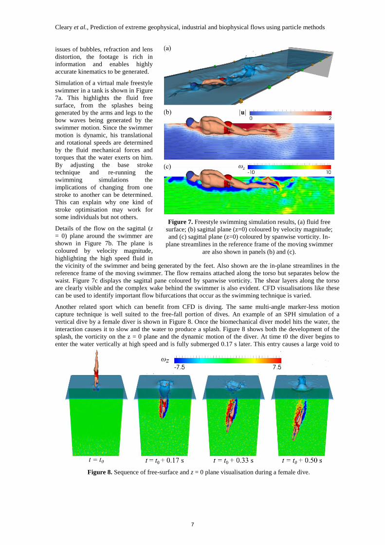
Simulation of a virtual male freestyle

swimmer in a tank is shown in Figure

7a. This highlights the fluid free

surface, from the splashes being

generated by the arms and legs to the

bow waves being generated by the

swimmer motion. Since the swimmer

motion is dynamic, his translational

and rotational speeds are determined

by the fluid mechanical forces and

torques that the water exerts on him.

By adjusting the base stroke

technique and re-running the

swimming simulations the

implications of changing from one

stroke to another can be determined.

This can explain why one kind of

stroke optimisation may work for

some individuals but not others.

Details of the flow on the sagittal (z

= 0) plane around the swimmer are

shown in Figure 7b. The plane is

coloured by velocity magnitude,

highlighting the high speed fluid in

the vicinity of the swimmer and being generated by the feet. Also shown are the in-plane streamlines in the

reference frame of the moving swimmer. The flow remains attached along the torso but separates below the

waist. Figure 7c displays the sagittal pane coloured by spanwise vorticity. The shear layers along the torso

are clearly visible and the complex wake behind the swimmer is also evident. CFD visualisations like these

can be used to identify important flow bifurcations that occur as the swimming technique is varied.

Another related sport which can benefit from CFD is diving. The same multi-angle marker-less motion

capture technique is well suited to the free-fall portion of dives. An example of an SPH simulation of a

vertical dive by a female diver is shown in Figure 8. Once the biomechanical diver model hits the water, the

interaction causes it to slow and the water to produce a splash. Figure 8 shows both the development of the

splash, the vorticity on the z = 0 plane and the dynamic motion of the diver. At time t0 the diver begins to

enter the water vertically at high speed and is fully submerged 0.17 s later. This entry causes a large void to

Figure 7. Freestyle swimming simulation results, (a) fluid free

surface; (b) sagittal plane (z=0) coloured by velocity magnitude;

and (c) sagittal plane (z=0) coloured by spanwise vorticity. In-

plane streamlines in the reference frame of the moving swimmer

are also shown in panels (b) and (c).

Figure 8. Sequence of free-surface and z = 0 plane visualisation during a female dive.

7


form in the water behind the descending diver. A further 0.16 seconds later the diver has slowed down

considerably and rotated off the vertical. Strong shear layers are visible around the body and the surrounding

water has rushed to fill the void. By time t0 + 0.50 s the diver has slowed down further and a large splash is

rising from the pool. Such modelling provides an ideal environment for studying different entry speeds, entry

angles and body positioning because the resultant motion and splashing can be objectively compared.

For both sports, much of the variability that needs to be coped with in the modelling relates to variation in the

athletes’ body deformation between repetitions, between training and competition, changes in their technique

with injury and fatigue and the very large variations that occur between athletes. There can also be large

variations in the conditions in which they perform (e.g. large waves from other competing swimmers).

6. BIOMEDICAL

The operation of biomedical systems often involves interactions between multi-phase fluids (blood, urine,

faeces) and surrounding soft tissues and muscle embedded in a dynamic biomechanical system that is the

human body. Two examples of biomedical applications where we have applied SPH are presented below.

6.1. Cardiac Flow Assistance (Axial Flow Pump)

Ventricular assist devices (VADs) are used as a temporary bridge-to-transplant for patients with congestive

heart failure, or as flow assistance for instances of heart disease where ventricular function is weakened. CFD

has been used in the heart pump industry for more than a decade, and is a well-established tool for pump

optimisation. To date, this has only involved grid-based methods and almost entirely focused on studying

steady flow conditions. However, models of transient flow are necessary for designers to understand the

velocity and pressure fluctuations occurring in a pump under unsteady flow conditions as would occur in a

clinical, in vivo setting. In addition, axial flow pump designs use very high rotor speeds (up to 10,000 rpm)

which can lead to significant haemolysis (red blood cell damage).

SPH offers some advantages over grid-based methods for pump applications in medicine. There is no need

for slip meshes to manage moving machine components, nor the potential mass and energy losses associated

with flow from moving meshes to stationary ones. In SPH, boundary geometries of almost arbitrary

complexity may be included such as intricate pump rotor geometry. SPH particles can also carry fluid history

easily, enabling inclusion of strain-based models for blood cell damage. Finally, SPH enables rule-based

modification of particles, meaning that one could also potentially model the growth of thrombi inside the

pump. Predictions of cell damage and clotting inside the pump are important for understanding the useful life

of a pump and pose significant challenges for grid-based methods.

Figure 9. Average a) tangential and b) axial flow velocities within the pump housing. Isosurfaces of axial

velocity (Vz) demonstrating retrograde flow in the pump for c) -0.2 m/s, and d) 1.0 m/s.

Sinnott and Cleary (2010) have used SPH to model flow through an axial flow pump (shown in Figure 9).

Figure 9a and b show the tangential and axial velocity flow field. Here, the impeller rotation draws blood

through the pump from right-to-left and converts the flow from linear motion (by the stationary inducer

blades) to rotational motion (by the rotating impeller blades) and back to linear (in the stationary diffuser)

with a subsequent rise in pressure head at the outlet of the pump. This is intended to approximate real cardiac

pressures. Isosurfaces of axial velocity are shown in Figure 9c (reverse flow) and Figure 9d (forwards flow)

and demonstrate recirculation inside the pump. Regions of recirculation are of concern for pump designers as

-0.2 m/s

1.0 m/s

b)

d)

a)

c)

8


they can trap blood inside the pump increasing the exposure time for red blood cells to significant levels of

shear and increasing the potential for blood damage.

6.2. Gastro-intestinal Transport

Controlled propulsion and mixing of content along the digestive tract is essential for a normal life. This is

achieved by a rich assortment of motor patterns that ensure that movements and propulsion are appropriate

for the breakdown of food, absorption of nutrients and excretion of waste. These movements (motility) are

due to coordinated contractions and relaxations of circular and longitudinal smooth muscle layers.

Computational modelling of gastrointestinal systems has the potential to help understand complex

relationships between flow and pressure for functional disorders where intestinal transport is abnormal.

However predicting the transient fluid-structure interactions which lead to large wall deformations poses

significant challenges for grid-based methods.

The mesh free nature of SPH means that large deformations can be modelled without requiring expensive and

diffusive re-meshing. Coupling of fluid/solid motion and wall deformation is captured naturally. Here, we

use SPH particles to model both the faecal content and the intestinal wall. Viscoelastic elements are

constructed between each pair of wall particles to allow the wall to flex in response to applied muscular

contractions and fluid pressures from the faecal content. This is a powerful and effective model for an active

boundary arising from the tightening or relaxing of circular muscle in the intestinal wall. The key advantage

of this model is that the instantaneous shape of the wall is a direct prediction from the fluid-structure

interaction between faecal content and muscular control of the boundary. This is in contrast with earlier

models (e.g. Pal et al. 2004) where the wall deformations were specified as inputs to the model thereby

introducing significant uncertainty about the predictive capability of such models.

Travelling peristaltic waves are generated in the intestinal wall and travel in the antegrade direction. The

wave consists of contraction (ascending excitation) and relaxation (descending inhibition, DI) components

that modify the instantaneous wall tensions in each longitudinal slice by controlling the natural lengths of the

elastic wall elements and thereby produces the required degree of contraction or relaxation. Complex

propagating sequences in the colon can easily be represented by series of these waves.

Figure 10 shows an example of peristaltic transport in the colon where the wave is travelling from left-to-

right. The downstream muscular relaxation (DI) was shown to be important for both transport and mixing by

Sinnott et al. (2011). A high pressure zone propagates immediately in front of the contraction such that fluid

wants to expand sideways. The addition of DI allows the walls to expand. Consequently there is a reduction

in luminal and intra-luminal pressures inside the region of DI which generates positive thrust for the fluid

volume contained inside the dilation region. This then travels forwards at the propagation speed of the

contraction. A recirculation vortex forms inside the DI (shown by the velocity field in Figure 10) that

influences the wall shape by controlling the pressure distribution, but the wall shape also influences the size

and shape of the vortex since they are coupled. The largest source of variability here are the details of the

peristaltic waves, which vary in timing, magnitude, degree of occlusion, location and speed. The waves can

also interact due to overlapping of wave effects due to their long relaxation times of the wall-fluid system.

Figure 10. Vertical slice through the centreline of the colon with faecal content (fluid) colour-shaded from

blue to red by pressure. Velocity arrows are coloured by longitudinal speed for antegrade (red) and retrograde

(blue) flow and the arrow length represents longitudinal speed.

9


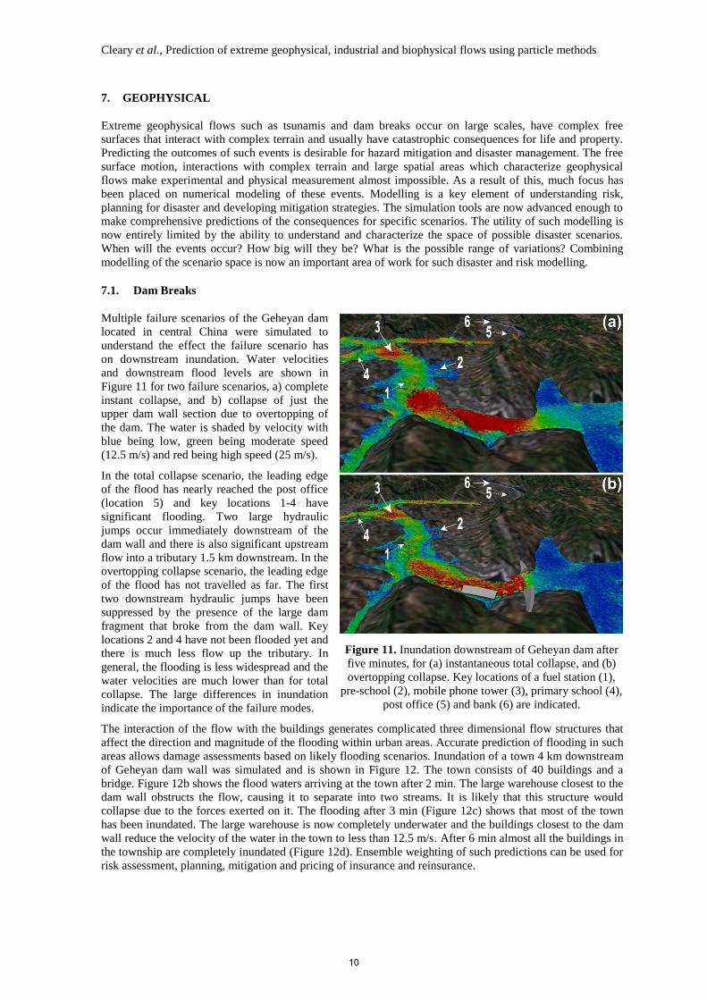
Figure 11. Inundation downstream of Geheyan dam after

five minutes, for (a) instantaneous total collapse, and (b)

overtopping collapse. Key locations of a fuel station (1),

pre-school (2), mobile phone tower (3), primary school (4),

post office (5) and bank (6) are indicated.

7. GEOPHYSICAL

Extreme geophysical flows such as tsunamis and dam breaks occur on large scales, have complex free

surfaces that interact with complex terrain and usually have catastrophic consequences for life and property.

Predicting the outcomes of such events is desirable for hazard mitigation and disaster management. The free

surface motion, interactions with complex terrain and large spatial areas which characterize geophysical

flows make experimental and physical measurement almost impossible. As a result of this, much focus has

been placed on numerical modeling of these events. Modelling is a key element of understanding risk,

planning for disaster and developing mitigation strategies. The simulation tools are now advanced enough to

make comprehensive predictions of the consequences for specific scenarios. The utility of such modelling is

now entirely limited by the ability to understand and characterize the space of possible disaster scenarios.

When will the events occur? How big will they be? What is the possible range of variations? Combining

modelling of the scenario space is now an important area of work for such disaster and risk modelling.

7.1. Dam Breaks

Multiple failure scenarios of the Geheyan dam

located in central China were simulated to

understand the effect the failure scenario has

on downstream inundation. Water velocities

and downstream flood levels are shown in

Figure 11 for two failure scenarios, a) complete

instant collapse, and b) collapse of just the

upper dam wall section due to overtopping of

the dam. The water is shaded by velocity with

blue being low, green being moderate speed

(12.5 m/s) and red being high speed (25 m/s).

In the total collapse scenario, the leading edge

of the flood has nearly reached the post office

(location 5) and key locations 1-4 have

significant flooding. Two large hydraulic

jumps occur immediately downstream of the

dam wall and there is also significant upstream

flow into a tributary 1.5 km downstream. In the

overtopping collapse scenario, the leading edge

of the flood has not travelled as far. The first

two downstream hydraulic jumps have been

suppressed by the presence of the large dam

fragment that broke from the dam wall. Key

locations 2 and 4 have not been flooded yet and

there is much less flow up the tributary. In

general, the flooding is less widespread and the

water velocities are much lower than for total

collapse. The large differences in inundation

indicate the importance of the failure modes.

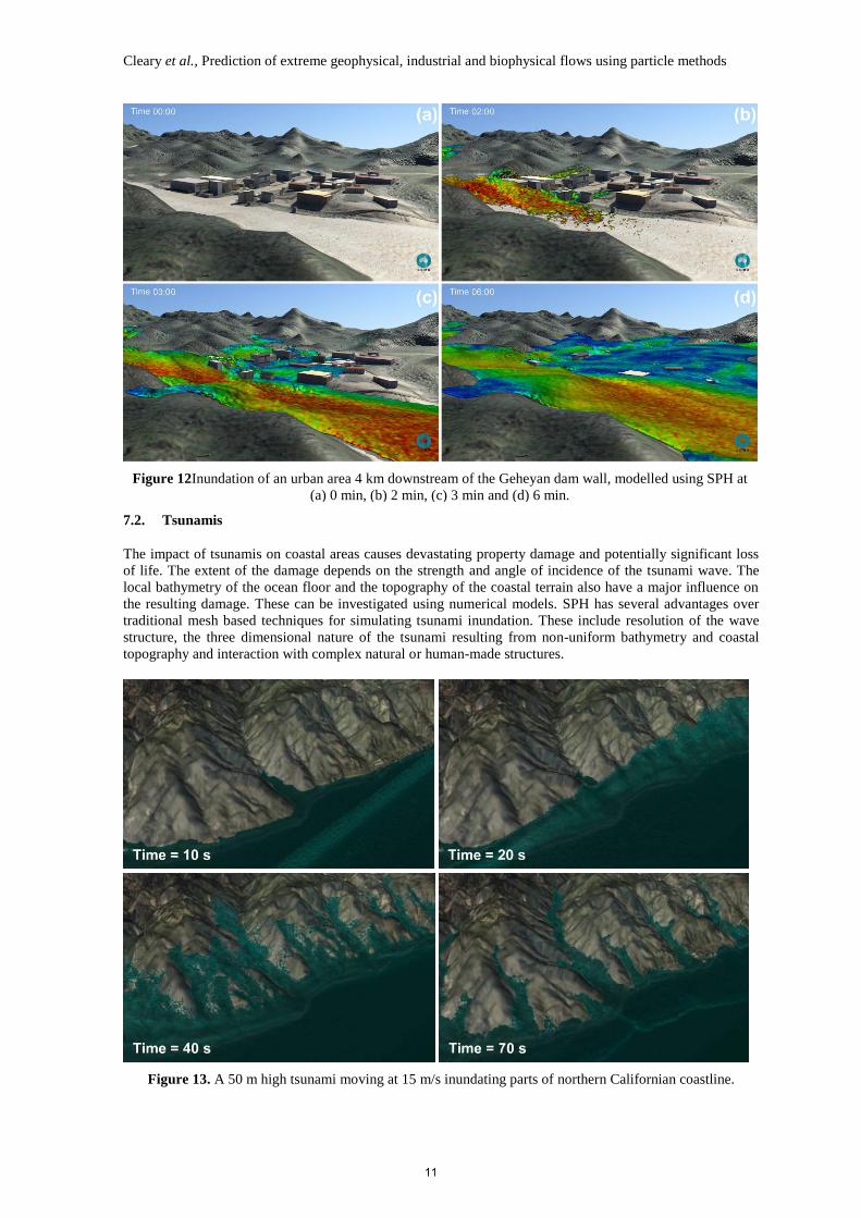
The interaction of the flow with the buildings generates complicated three dimensional flow structures that

affect the direction and magnitude of the flooding within urban areas. Accurate prediction of flooding in such

areas allows damage assessments based on likely flooding scenarios. Inundation of a town 4 km downstream

of Geheyan dam wall was simulated and is shown in Figure 12. The town consists of 40 buildings and a

bridge. Figure 12b shows the flood waters arriving at the town after 2 min. The large warehouse closest to the

dam wall obstructs the flow, causing it to separate into two streams. It is likely that this structure would

collapse due to the forces exerted on it. The flooding after 3 min (Figure 12c) shows that most of the town

has been inundated. The large warehouse is now completely underwater and the buildings closest to the dam

wall reduce the velocity of the water in the town to less than 12.5 m/s. After 6 min almost all the buildings in

the township are completely inundated (Figure 12d). Ensemble weighting of such predictions can be used for

risk assessment, planning, mitigation and pricing of insurance and reinsurance.

10


7.2. Tsunamis

The impact of tsunamis on coastal areas causes devastating property damage and potentially significant loss

of life. The extent of the damage depends on the strength and angle of incidence of the tsunami wave. The

local bathymetry of the ocean floor and the topography of the coastal terrain also have a major influence on

the resulting damage. These can be investigated using numerical models. SPH has several advantages over

traditional mesh based techniques for simulating tsunami inundation. These include resolution of the wave

structure, the three dimensional nature of the tsunami resulting from non-uniform bathymetry and coastal

topography and interaction with complex natural or human-made structures.

Figure 13. A 50 m high tsunami moving at 15 m/s inundating parts of northern Californian coastline.

Figure 12Inundation of an urban area 4 km downstream of the Geheyan dam wall, modelled using SPH at

(a) 0 min, (b) 2 min, (c) 3 min and (d) 6 min.

11


Figure 13 shows a 50 m high tsunami wave moving at 15 m/s inundating parts of the northern Californian

coastline. At 10 s, the wave is approaching the coastline from the southwest at a 30° angle, with the southern

sections beginning to be inundated. At 20 s, the wave has now impacted the entire length of the coastline.

The water has started moving inland in the southern section. By 40 s, the water has moved 1.5 km inland. At

70 s, the water has started receding from the southern sections but is still moving further inland along the

central and northern sections. The water has inundated around 2 km inland along the central valley and is

now approaching its maximum levels. The detailed predictions of such a deterministic model can be used

within a risk frame work to determine the consequences for the different scenarios considered.

8. CONCLUSIONS

Particle based computational methods have a range of strong advantages over traditional grid based

continuum methods. These include:

the ability to include particle level information in collision dominated particle flows

ability to resolve complex fluid free surfaces including splashing and fragmentation

ability to predict very large deformations, including fracture and interaction with moving objects

ability to track material history and use this in the flow modelling.

These have been demonstrated in a broad range of computationally demanding applications including

comminution, biomedical, geophysical extreme flow events (risk/disaster modelling), eating of food by

humans and elite water based sports. In all cases, there are significant sources of variability that need to be

taken into account in the modelling. For human based models the major sources of variability are the nature

of the motions of the human (both internal and external). For the disaster modelling, the variability is mainly

reflected in the range and nature of scenarios that need to be considered in building risk frameworks in which

these models can predict specific consequences. Finally, in all the applications there is commonly uncertainty

about material properties and the details of the initial conditions whose affects need to be understood.

ACKNOWLEDGMENTS

The authors acknowledge the financial and material contributions of the Aquatics Testing, Training and

Research Unit (ATTRU) at the Australian Institute of Sport (AIS) to the human swimming research.

REFERENCES

Campbell, C. S. (1990). Rapid granular flows. Annual Review Fluid Mechanics 22, 57-92.

Cleary, P. W. (2004). Large scale industrial DEM modelling. Engineering Computations 21, 169-204.

Cleary, P. W. (2009). Industrial particle flow modelling using DEM. Engineering Computations 26, 698-743.

Cleary, P. W., Prakash, M., Ha, J., Stokes, N., and Scott, C. (2007). Smooth Particle Hydrodynamics: Status

and future potential, Progress in Computational Fluid Dynamics, 7, 70-90.

Cohen, R. C. Z., Cleary, P. W., and Mason, B. R. (2011). Simulations of dolphin kick swimming using

smoothed particle hydrodynamics.Human Movement Science. doi:10.1016/j.humov.2011.06.008.

Cundall, P. A., and Strack, O. D. L. (1979). A discrete numerical model for granular assemblies.

Geotechnique. 29, 47-65.

Dejak, B., Mlotkowski, A., and Romanowicz, M. (2003) Finite element analysis of stresses in molars during

clenching and mastication. The Journal of Prosthetic Dentistry, 90(6), 591-597

de Loubens, C., Saint-Eve, A. l ris I. anouill , M., Doyennette, M. Tr l a, I.C., and Souchon, I.. (2011)

Mechanistic model to understand in vivo salt release and perception during the consumption of dairy gels.

Journal of Agricultural and Food Chemistry, 59(6), 2534-2542.

Haff, P. K., and Werner, B. T. (1986). Computer simulation of the mechanical sorting of grains. Powder

Technology. 48, 239.

Monaghan, J. J. (1994). Simulating free surface flows with SPH. J. Computational Physics 110, 399-406.

Pal, A., Indireshkumar, K., Schwizer, W., Abrahamsson, B., Fried, M., and Brasseur, J. (2004). Gastric flow

and mixing studied using computer simulation, Proceedings Royal Society. London B, 271, 2587-2594.

Sinnott, M., Cleary, P.W., Arkwright, J., and Dinning, P. (2011). Investigating the relationships between

peristaltic contraction and fluid transport in the human colon using Smoothed Particle Hydrodynamics.

Computers in Biology and Medicine. Submitted in 2011.

Sinnott, M., and Cleary, P.W. (2010). Effect of rotor blade angle and clearance on blood flow through a non-

pulsatile, axial, heart pump. Progress in Computational Fluid Dynamics, 10, 300-306.

Walton, O. R. (1994). Numerical simulation of inelastic frictional particle-particle interaction, Chapter 25 in:

Particulate two-phase flow, ed. M. C. Roco, pp. 884-911, Boston: Butterworth-Heinemann.

12

Documents

Prediction of extreme geophysical, industrial and biophysical