HOSTED BY Available online at www.sciencedirect.com

ScienceDirect

Natural Gas Industry B 2 (2015) 283e294www.elsevier.com/locate/ngib

Research article

Prediction of gas compressibility factor using intelligent models

Mohamadi-Baghmolaei Mohamada, Azin Rezab,*, Osfouri Shahriara,Mohamadi-Baghmolaei Rezvanc, Zarei Zeinaba

a Department of Chemical Engineering, Faculty of Petroleum, Gas and Petrochemical Engineering, Persian Gulf University, Bushehr, Iranb Department of Petroleum Engineering, Faculty of Petroleum, Gas and Petrochemical Engineering, Persian Gulf University, Bushehr, Iran

c Department of Computer Science and Engineering and Information Technology, School of Electrical Computer Engineering, Shiraz University, Shiraz, Iran

Received 23 July 2015; accepted 7 September 2015

Available online 27 November 2015

Abstract

The gas compressibility factor, also known as Z-factor, plays the determinative role for obtaining thermodynamic properties of gas reservoir.Typically, empirical correlations have been applied to determine this important property. However, weak performance and some limitations ofthese correlations have persuaded the researchers to use intelligent models instead. In this work, prediction of Z-factor is aimed using differentpopular intelligent models in order to find the accurate one. The developed intelligent models are including Artificial Neural Network (ANN),Fuzzy Interface System (FIS) and Adaptive Neuro-Fuzzy System (ANFIS). Also optimization of equation of state (EOS) by Genetic Algorithm(GA) is done as well. The validity of developed intelligent models was tested using 1038 series of published data points in literature. It wasobserved that the accuracy of intelligent predicting models for Z-factor is significantly better than conventional empirical models. Also, resultsshowed the improvement of optimized EOS predictions when coupled with GA optimization. Moreover, of the three intelligent models, ANNmodel outperforms other models considering all data and 263 field data points of an Iranian offshore gas condensate with R2 of 0.9999, while theR2 for best empirical correlation was about 0.8334.© 2015 Sichuan Petroleum Administration. Production and hosting by Elsevier B.V. This is an open access article under the CC BY-NC-NDlicense (http://creativecommons.org/licenses/by-nc-nd/4.0/).

Keywords: Z-factor; Gas condensate; Empirical correlation; Intelligent models

1. Introduction

Obtaining fluid properties from gas and oil reservoirs hasbeen of great importance to many researchers and petroleumengineers. The significance of this knowledge becomes morebrilliant when the oil and gas capacity of reservoirs, dissolvedgas, aquifer model and other reservoir properties dependsdirectly or indirectly on fluid properties [1]. For this purpose,the pressure, volume and temperature (PVT) analysis shouldbe applied to find the aforementioned parameters. This can bemade in PVT laboratory or by using proper correlations [2].

* Corresponding author. Tel.: þ98 9177730085; fax: þ98 7733441495.

E-mail address: reza.azin@pgu.ac.ir (Azin R.).

Peer review under responsibility of Sichuan Petroleum Administration.

http://dx.doi.org/10.1016/j.ngib.2015.09.001

2352-8540/© 2015 Sichuan Petroleum Administration. Production and hosting by

(http://creativecommons.org/licenses/by-nc-nd/4.0/).

For the case of gas condensate and gas reservoir, estimationof Z-factor plays a key role for determination of other prop-erties. Obtaining the accurate Z-factor has been the subject ofcontroversy among researchers. High expenses and inacces-sibility to some well-equipped laboratories are the reasons forresearchers to be reluctant to use the direct measurement of Z-factor. The common ways for prediction of Z-factor are EOSand empirical correlations. The EOS have been developed andextended for vapor liquid equilibrium (VLE) calculations [3],estimation of critical properties [4] and prediction of volu-metric properties of gas mixture as well [5,6]. The point thatshould be considered about EOS is that despite the accurateresults attained from developed and modified EOS in com-parison to empirical correlations, a bit more difficulties areinvolved in solution process and more involving parametersare dealt with. On the other hand, the foible point of empirical

Elsevier B.V. This is an open access article under the CC BY-NC-ND license

284 Mohamadi-Baghmolaei M. et al. / Natural Gas Industry B 2 (2015) 283e294

correlations is that they are usually developed based on spe-cific data set. A good illustration is Sanjari and Lay investi-gation which concluded to an empirical correlation for Z-factor using Khangiran Refinery data set [7]. Another exampleis Heidarian et al. study on gas compressibility factor whichled to empirical correlation based on limited experimentaldata [8]. Likewise, Azizi et al. [9]generated a correlationusing extracted data from Standing-Katz chart [10] or inves-tigation of Farzaneh-Gord and Rahbari [11]who usedmeasurable real time properties for developing the empiricalcorrelation. An interesting example is Jarrahian and Heidarian[12] study in which they proposed a new EOS for sour andsweet natural gases when the composition is unknown. Theytried to lessen the input variables in compare to otherempirical correlations.

The fundamental tool for estimation of thermophysicalproperties of hydrocarbon fluids is EOS. Overall, EOS havetheir own mixing rules which cause complexity in solutionprocess. The EOS based on statistical-mechanical theory yieldmore accurate results. On the other hand, empirical correla-tions are widely used in petroleum engineering applicationssimply as they are practical and easy to use. That is to say, thechief reason which makes the petroleum engineers tend to dealwith these kind of correlations is that they are explicit in Zwith straight forward solution procedure [13].

The complexity of EOS makes them difficult to applyespecially for mixtures with large number of components.Also, questionable and unreliable predictions of Z-factor usingempirical correlations at some pressures and temperatureshave led the researchers to seek for easier, more reliable andvalid prediction for z-factor. On the other hand, application ofintelligent models becomes important to compensate weaknessof conventional methods. The intelligent systems are widelyused as robust tools to predict the petroleum properties andalso other engineering parameters [14e16]. A good exampleof using intelligent models in reservoir engineering is Saemiet al. work [17], in which they predicted reservoir permeabilityusing linked Adaptive Neural Network and Genetic Algorithm(GA). Other examples of intelligent models usage in reservoirfluid properties are prediction of bubble point pressure byANN [18], minimum miscibility pressure (MMP) by leastsquare support vector machine (LSSVM) [19], dew pointpressure using Fuzzy Logic model [20], Z-factor of natural gas[21] and sour gasusing Adaptive Neuro Fuzzy Inference Sys-tem (ANFIS) and ANN model [22] and condensate to gas ratioby LSSVM model [23]. In another study, Ganji-Azad et al.applied the ANFIS model to predict reservoir fluid PVTproperties [24]. Moreover, Fayazi et al. [25] and Rafiee-Taghanaki [26] proposed a robust model for prediction ofgas compressibility factor by application LSSVM.

In this study, experimental PVT data of gas condensatereservoir are used to compare and analyze accuracy ofempirical correlations and EOS coupled with intelligentmodels. In the following sections, the application of intelli-gent models will be presented in two parts. The first partincludes improvement and optimization of Van Der Waals

and Redlich Kwong equation of state by implementation ofexperimental data using Genetic Algorithm [27]. Second partis allocated to employ the Fuzzy Logic (FIS), ANFIS andANN predicting models and suggest the best intelligentmodel for predicting gas Z-factor. These intelligent modelsare trained by share of experimental data, while the remain-ing data are used for validation and test. Some of theseintelligent models are utilized to predict the gas Z-factor inprevious works, and their ability will be evaluated andcompared with empirical correlations comprehensively in thecurrent study.

2. Empirical correlations and equations of state

2.1. Empirical equations

Several empirical correlations have been developed yet topredict Z-factor. These correlations relate the critical proper-ties of mixture, temperate and pressure of reservoir to the Z-factor.

The regression approach is frequently used to generateempirical correlations such as that of Sanjari and Lay (SL) in2012. They generated an empirical predicting correlation ofgas compressibility. They have developed their correlationbased on Virial equation of state. They proposed correlation asa function of ppr and Tpr within the range of 0:01 � ppr � 15and 1:01 � Tpr � 3 [7].

Z ¼ 1þA1ppr þA2ppr2 þA3pprA4

TprA5þA6pprA4þ1

TprA7þ A8pprA4þ2

TprðA7þ 1Þð1Þ

Many empirical correlations are adjusted by pseudoreduced temperature and pressure such as that of Shell OilCompany (SOC) which was referenced by Kumar [28].

Z ¼ AþBppr þ ð1�AÞexpð�CÞ �D�ppr10

�4ð2Þ

2.2. Equations of state

Generally, cubic EOS originated from Van Der Waalsequation of state are more applicable for industrial proposes[29]. These EOS are commonly rewritten in cubic polynomialform. Vander Waals (VdW) equation is the basic cubic EOSwhich modified the ideal gas PVT relations [30]. The cubicpolynomial form of VdW EOS, equation (8), can be solved tofind the Z-factor:

Z3 � ð1þBÞZ2 þAZ �AB¼ 0 ð3Þwhere, A ¼ ap

R2T2 and B ¼ bpRT. The coefficients a and b are

defined as follow:

a¼ 0:421875R2T2

c

pcð4Þ

Fig. 1. Schematic of MLP structure.

Fig. 2. The structure of ANFIS model.

285Mohamadi-Baghmolaei M. et al. / Natural Gas Industry B 2 (2015) 283e294

b¼ 0:125RTc

pcð5Þ

Redlich and Kwong (RK) in 1949 improved the VdW EOSto predict more accurate compressibility of vapor phase. Theyconsidered a generalized temperature dependence term asmodification of attraction pressure term in their correlation[31].

Z3 � Z2 þ �A�B�B2�Z �AB¼ 0 ð6Þ

where, A ¼ apR2T2:5 and B ¼ bp

RT. The coefficients a and b areobtained by equations 12 and 13:

a¼ 0:42747R2T2:5

c

pcð7Þ

b¼ 0:08664RTc

pcð8Þ

The evolutionary path of VdW type EOS has reached toSoave-Redlich-Kwong (SRK) equation of state in 1972 andPeng-Robinson (PR) equation in 1976 [32,33]. For the cases inwhich the composition of gas mixture is unknown (like thisstudy), the use of SRK and PR equation of state is impossible.

3. Intelligent models

The chief purpose of an intelligent software is to bridge setsof input and output variables to each other considering thesystem specifications [34]. Application of intelligent-basedmodels is more efficient in such cases which are timeconsuming and involve non-linear mathematical modeling,adaptive learning and when there is not any meaningful rela-tion between input and output of a system. The intelligentmodels developed in this study include ANN, ANFIS(including FIS) and GA.

3.1. Artificial Neural Network

Table 1

Statistical information of data points.

Property Max. Min. Avg. SDa

Temperature/R 681.03 515.07 615.653 56.133

Pressure/psia 9104.536 1175.69 5391.07 1390.637

Z-factor 1.374 0.71 0.9896 0.1159

Tpc/R 427.2004 385.4219 4.09Eþ02 1.03Eþ01

ppc/psia 663.6487 650.0807 6.67Eþ02 1.56Eþ00

MW 2.62Eþ01 2.06Eþ01 2.21Eþ01 9.74E-01

Specific volume/m3 kg�1 1.46E-02 2.34E-03 3.81E-03 1.65E-03

Gas gravity 9.06E-01 7.11E-01 7.63E-01 3.38E-02

a denotes Standard deviation.

An ANN is a network of interconnected nodes exhibitingthe process of biological neurons in a brain. The artificialneurons lie in constitutive layers of the network. Each layer islinked to the next by specific weights (w) [35]. One of the mostpractical structures of ANN is Multi-Layer Perceptron (MLP)in which the input and output layers are connected to eachother by an additional layer called hidden layer. The hiddenlayers do the processing step and output layer gathers thesignals and distributes [36]. A MLP network may have one ormore hidden layers; however, it is seen that a network with onehidden layer can predict the performance of a system as well[15]. The network adopts the weights of neurons based onerror between outputs and targets in training steps. Moreover,for constructing robust design, some of unused data in trainingstep are used for validation, which makes the model moreaccurate. The structure of ANN is illustrated in Fig. 1.

It is seen from figure that the networks consist of threelayers i, j and k where the weights between layers is desig-nated by wij and wjk. The initial weighted values are modified

during training process by the comparison made betweenpredicted and real values [37]. Among various training algo-rithm Levenberg-Marquart (LM) is commonly used fortraining system due to its stability and swift convergence [38].In the current study, the LM algorithm will be utilized wherethe weights are computed by:

Wkþ1 ¼Wk �hJTWk

JWkþ mkI

i�1

*JTWkVWkð9Þ

where the weighted matrix are symbolized by Wkþ1 and WK

during K þ 1th and Kth repetitions, J is the Jacobian matrix, Vis the accumulated errors vector, I is the identity matrix, and mkis the parameter to express the ability of LM algorithm foraltering the searching method. In the present study, the input

Table 2

Calculated errors of empirical correlations considering all experimental data.

R2 ARE % AARE % RMSE RSS MSE

BB 0.833467 1.855974 3.670279 0.001201 0.612853 0.002403

DA 0.7476682 0.2914712 3.9412058 0.0015169 0.7736368 0.0030338

HY 0.830662 2.992630 4.030546 0.001338 0.682459 0.002676

HD 0.8330268 3.0963429 3.9694283 0.0012782 0.6519107 0.0025565

PP 0.379220 17.39785 18.12433 0.038935 19.85726 0.077871

SL 0.7956868 3.1706066 4.2371119 0.0016540 0.8435509 0.00330804

SOC 0.7903665 0.7361394 5.1792569 0.0023512 1.1991327 0.0047024

286 Mohamadi-Baghmolaei M. et al. / Natural Gas Industry B 2 (2015) 283e294

layer L is consist of three variables which are Tpr, ppr and ggalso output layer K is allocated to target value, i.e. Z-factor.

3.2. Adaptive Neuro-Fuzzy Inference System (ANFIS)

Table 3

Modification of EOS coefficients using GA.

a b Modified a Modified b

The ANFIS is the combination of neural networks andfuzzy modeling in training step in order to improve the abilityof learning [39]. The ANFIS applies the beneficial features ofANN and fuzzy model by a hybrid structure and modifies theinappropriate properties. In other words, ANFIS combines thelow level calculation of ANN and the powerful reasoningability of a fuzzy logic system. Based on ANFIS modeling fornon-linear systems, the input space is divided into many localareas. In this regard, the modest local is developed by linearfunctions or adjustable coefficients; next the ANFIS uses themembership function (MF) to determine the dimension ofeach input. Hence, the MFs and the hidden layers play a keyrole in estimation of ANFIS model ability. The five layers ofANFIS modeling is shown in Fig. 2 [39].

The adaptive nodes of the first layers are equated as:

mAiðxÞ ¼ exp�

�x�x*

s2

�ð10Þ

where x* and ơ* are premise parameters which are adapted bya hybrid algorithm and x is the input variable. In the presentstudy, the three input variables are Tpr, ppr and gg.

Fig. 3. Comparison between the best empirical correlation and experimental

data.

The firing strength of each rule is determined in the secondlayer by quantifying the extent of each rule's input data. Theoutput of a layer is the algebraic product of input signals:

O2;i ¼ ui ¼ mAiðx1Þ �…� mCiðxnÞ ð11ÞThe third layer is responsible of normalization by calcu-

lating ratio of ith rule's firing strength to the summation resultof all rule's firing strength:

O3;i ¼ ui ¼ ui

ðui þ…þunÞ ð12Þ

The calculation of output is done by the fourth layer:

O4;i ¼X

uifi ð13Þ

where the total output is obtained as the summation of all inputsignals in the fifth layer by calculation of wave height asfollow [40]:

O5;i ¼Pn

i¼1uifiPni¼1ui

ð14Þ

O5,i is Z-factor in this study.

VdW 0.421875 0.125 0.3619423 0.1016583

RK 0.42747 0.08664 0.4995234 0.0897378

Fig. 4. Z-factor variation versus pressure at 667.67 R for all 263 data points.

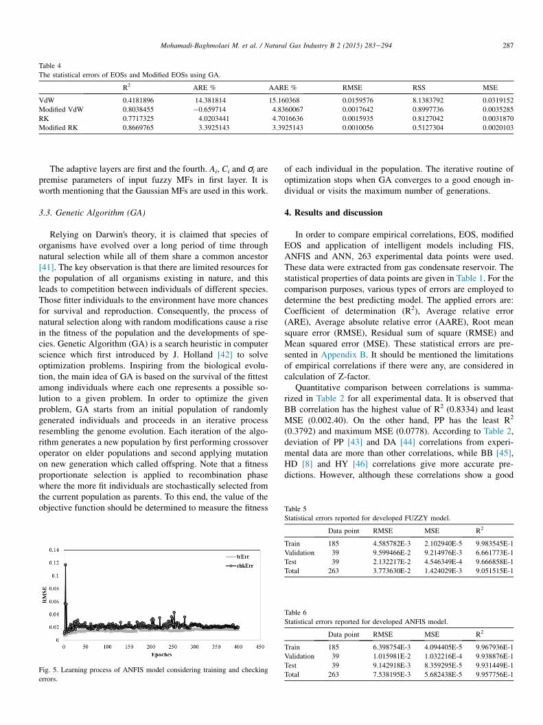
Table 4

The statistical errors of EOSs and Modified EOSs using GA.

R2 ARE % AARE % RMSE RSS MSE

VdW 0.4181896 14.381814 15.160368 0.0159576 8.1383792 0.0319152

Modified VdW 0.8038455 �0.659714 4.8360067 0.0017642 0.8997736 0.0035285

RK 0.7717325 4.0203441 4.7016636 0.0015935 0.8127042 0.0031870

Modified RK 0.8669765 3.3925143 3.3925143 0.0010056 0.5127304 0.0020103

287Mohamadi-Baghmolaei M. et al. / Natural Gas Industry B 2 (2015) 283e294

The adaptive layers are first and the fourth. Ai, Ci and ơi arepremise parameters of input fuzzy MFs in first layer. It isworth mentioning that the Gaussian MFs are used in this work.

3.3. Genetic Algorithm (GA)

Table 5

Relying on Darwin's theory, it is claimed that species oforganisms have evolved over a long period of time throughnatural selection while all of them share a common ancestor[41]. The key observation is that there are limited resources forthe population of all organisms existing in nature, and thisleads to competition between individuals of different species.Those fitter individuals to the environment have more chancesfor survival and reproduction. Consequently, the process ofnatural selection along with random modifications cause a risein the fitness of the population and the developments of spe-cies. Genetic Algorithm (GA) is a search heuristic in computerscience which first introduced by J. Holland [42] to solveoptimization problems. Inspiring from the biological evolu-tion, the main idea of GA is based on the survival of the fittestamong individuals where each one represents a possible so-lution to a given problem. In order to optimize the givenproblem, GA starts from an initial population of randomlygenerated individuals and proceeds in an iterative processresembling the genome evolution. Each iteration of the algo-rithm generates a new population by first performing crossoveroperator on elder populations and second applying mutationon new generation which called offspring. Note that a fitnessproportionate selection is applied to recombination phasewhere the more fit individuals are stochastically selected fromthe current population as parents. To this end, the value of theobjective function should be determined to measure the fitness

Fig. 5. Learning process of ANFIS model considering training and checking

errors.

of each individual in the population. The iterative routine ofoptimization stops when GA converges to a good enough in-dividual or visits the maximum number of generations.

4. Results and discussion

In order to compare empirical correlations, EOS, modifiedEOS and application of intelligent models including FIS,ANFIS and ANN, 263 experimental data points were used.These data were extracted from gas condensate reservoir. Thestatistical properties of data points are given in Table 1. For thecomparison purposes, various types of errors are employed todetermine the best predicting model. The applied errors are:Coefficient of determination (R2), Average relative error(ARE), Average absolute relative error (AARE), Root meansquare error (RMSE), Residual sum of square (RMSE) andMean squared error (MSE). These statistical errors are pre-sented in Appendix B. It should be mentioned the limitationsof empirical correlations if there were any, are considered incalculation of Z-factor.

Quantitative comparison between correlations is summa-rized in Table 2 for all experimental data. It is observed thatBB correlation has the highest value of R2 (0.8334) and leastMSE (0.002.40). On the other hand, PP has the least R2

(0.3792) and maximum MSE (0.0778). According to Table 2,deviation of PP [43] and DA [44] correlations from experi-mental data are more than other correlations, while BB [45],HD [8] and HY [46] correlations give more accurate pre-dictions. However, although these correlations show a good

Statistical errors reported for developed FUZZY model.

Data point RMSE MSE R2

Train 185 4.585782E-3 2.102940E-5 9.983545E-1

Validation 39 9.599466E-2 9.214976E-3 6.661773E-1

Test 39 2.132217E-2 4.546349E-4 9.666858E-1

Total 263 3.773630E-2 1.424029E-3 9.051515E-1

Table 6

Statistical errors reported for developed ANFIS model.

Data point RMSE MSE R2

Train 185 6.398754E-3 4.094405E-5 9.967936E-1

Validation 39 1.015981E-2 1.032216E-4 9.938876E-1

Test 39 9.142918E-3 8.359295E-5 9.931449E-1

Total 263 7.538195E-3 5.682438E-5 9.957756E-1

Fig. 6. Variation MSE values versus training Epoches.

288 Mohamadi-Baghmolaei M. et al. / Natural Gas Industry B 2 (2015) 283e294

agreement with experimental data, they do not convince thepetroleum engineering needs for predicting the accurate andreliable Z-factor.

Comparison of experimental data and BB model as the bestpredicting correlation for all 263 data points is shown in Fig. 3by scatter diagram. The BB model shows the closest agree-ment with experimental data; however, predicted results arestill far from the set point data.

As the gas mixture components and their acentric factorsare not available, the VdW and RK EOS were optimized usingGA. To do this, results of VdW and RK EOS were chosen asfitness functions. The fitness functions have been comparedwith experimental data to reach the optimum results. Theobjective functions were function of four variables, i.e. tem-perature, pressure, pseudo critical temperature and pressure. It

Fig. 7. Comparison of output and target values related to training, validation

and test.

is worth noting that 50 generations were used to find the op-timum results which are two coefficients of EOS. The Modi-fied coefficients are summarized in Table 3. Effects ofmodification on VdW and RK EOS are shown in Fig. 4, wherethe variations of Z-factor versus pressure are displayed.

The statistical errors are reported in Table 4. As seen, theR2 improved from 0.4181 to 0.8038 and from 0.7717 to 0.8669for VdW and RK EOS, respectively as a result of GA opti-mization. Accordingly, the least values of AARE and MSEerrors belong to Modified RK, which are 3.3925 and 0.002respectively. On the other hand, the VdW EOS allocates themaximum AARE and MSE errors 15.1603 and 0.0319. It isclear from Fig. 5 and Table 4 that the accuracy of results fromVdW EOS is much less than those of RK equation. Theconsiderable difference between concluded results from twomethods still remains even after the modification.

4.1. Development of ANFIS

The developed ANFIS is used to present an intelligentpredicting model for Z-factor. In fact, the ANFIS system is acombination of FIS and ANN model. In other words, theFuzzy model parameters are being optimized by NeuralNetwork. The ANFIS model compensates some weaknesses ofFIS system. The Sugeno-type Fuzzy Inference System settlesdown to present a predicting model using training data withoutany check and testing. Therefore, it is common to tune themodel with the least error in training step, but unusual errors intests and validation steps which results in error propagation. Inother words, if there is any checking step, it will prevent overfitting the model on training data.

The Sugeno-type Fuzzy Interface System generates clustersfor introducing its rules. Therefore, determining the radius ofclusters, which specifies the number of clusters, is essential inobtaining the number of rules and developing the Fuzzymodel. The less radius results more clusters and also morerules. In other words, the larger the radius, the less is thenumber of clusters.

For this study, all 263 series of data points were firstrandomly divided in three parts where 70% of whole data usedfor training, 15% for validation and 15% for test. Next, theSugeno-type Fuzzy system was generated using 70% of wholedata which were trained. For this purpose, the initial radius ofinput data, which are temperature, pressure and specific gasgravity, should be determined. The applied initial input vari-ables were 5, 0.5, 0.05 for temperature, pressure and specificgas gravity respectively and also 0.05 for Z-factor which isoutput variable. The statistical errors related to Fuzzy

Table 7

Statistical errors reported for developed ANN model.

Data point MSE R2

Train 185 0.11031E-10 0.99999

Validation 39 9.12044E-10 0.99999

Test 39 5.26094E-08 0.99999

Total 263 8.75017E-09 0.99999

Fig. 8. Comparison of experimental data and ANN results.

Table 8

Comparison of statistical errors corresponded to three intelligent models.

R2 ARE/% AARE/% RMSE RSS MSE

FIS 0.90183886 �0.1846262 0.71927844 7.458890E-4 0.380403403 0.001491778

ANFIS 0.99577559 �0.0395657 0.42042680 2.841218E-5 0.014490215 5.6824372E-5

ANN 0.99999999 7.6890E-04 0.00223901 1.92894E-09 9.83761E-07 8.75017E-09

Table 9

Properties of other data base extracted from literature.

Ref. Data points No. Gas mixtures P/psia T/R MW Z

[48] 47 5 97.02e1106.90 558.36e646.92 51.56e16.60 0.86e0.99

[49] 165 5 1039.29e7120.68 559.67e619.66 23.67e18.17 0.67e1.14[50] 100 4 3238.41e1747.83 545.76e753.48 17.05e20.51 1.28e2.04

[51] 84 3 145.53e2207.94 455.67e581.67 16.31e17.85 0.59e0.94

[52] 234 2 1470.00e17125.50 563.76e795.24 17.09e16.35 0.92e1.42

[53] 241 3 132.20e2950.29 432.00e720.12 18.43e17.24 0.64e1.91[54] 105 5 1039.29e7120.68 560.77e620.76 20.85e18.80 0.71e1.14

[55] 61 6 98.49e1265.67 509.65e599.70 29.92e31.30 0.66e0.99

Total 1038 33

289Mohamadi-Baghmolaei M. et al. / Natural Gas Industry B 2 (2015) 283e294

290 Mohamadi-Baghmolaei M. et al. / Natural Gas Industry B 2 (2015) 283e294

predicting model is reported in Table 5. As seen, the maximumR2 belongs to training section as expected, and the least valuefor validation. It is worth noting that the most important typeof reported error is that of check or test which determine theability of model for new unused data while the validity errorshows the generality of proposed model. The R2 value of0.9051 obtained from Fuzzy model is more than that of bestempirical correlation and modified RK EOS; however, pre-dicted values do not match the target values with highaccuracy.

In order to improve the ability of FIS predicting model, thegenerated Fuzzy model parameters were optimized by ANN.The ANFIS model considers 70% of data for training and the15% for validation and the remains for test. It should bementioned that the three parts of implemented data werecompletely explicit and there was not any mutual node in threeparts. The learning process of ANFIS model along withconsidering training and checking errors is shown in Fig. 5which indicates that the values of errors in training andchecking steps are close to each other at the end of process.

The statistical errors of output ANFIS model are reported inTable 6. It is seen that total R2 value (0.99577) is more thanthat of FIS model where the MSE value of Fuzzy model(1.42E-3) was reduced to 5.683E-5. Results of Table 6 indicatethat the proposed model works better in comparison to othermethods for prediction of Z-factor.

Table 10

Comparison of AARE of intelligent system with other predicting model using rep

Ref. AARE/%

PP SL DA HD

[48] 0.87 0.32 14.71 0.55

[49] 5.40 1.52 9.69 2.36

[50] 85.62 6.04 5.52 35.57

[51] 32.10 1.28 20.12 1.33

[52] 24.78 1.58 1.56 2.41

[53] 1.46 0.94 13.14 2.09

[54] 7.32 2.00 8.96 2.47

[55] 2.044 1.28 33.42 0.9116

Total 159.59 14.96 107.12 47.69

Table 11

Comparison of MSE of intelligent system with other predicting model using repo

Ref. MSE

PP SL DA HD

[48] 9.97E-05 2.14E-05 0.0202 4.29E-05

[49] 0.0088 3.33E-04 0.0098 5.89E-04

[50] 2.5694 0.0191 0.0214 0.4589

[51] 0.1175 2.84E-04 0.0329 1.39E-04

[52] 0.1936 4.82E-04 5.02E-04 9.65E-04

[53] 0.0042 0.004 0.0209 0.0043

[54] 0.0144 5.90E-04 0.0091 8.52E-04

[55] 5.88E-04 3.44E-04 0.1353 3.50E-04

Total 2.91 2.52E-02 0.25 0.466

4.2. Development of ANN

For developing the ANN model, all 263 series of data pointwere normalized between 0 and 1. The input variables arepressure, temperature and specific gas gravity, and Z-factor isconsidered as a function of these parameters:

Z ¼ f�T ;p;gg

� ð17ÞIt is worth mentioning that selection of input variables af-

fects the reliability and performance of any predicting model;hence, it should reflect the physical properties and the natureof system. The network consists of two layers, i.e. input layerand hidden layers. The input layer included three nodsregarding temperature, pressure and gas gravity. These nodesare bridged to the hidden layer by specific weights. This layeris responsible for the main data processing. On the other hand,the output of this network has one nod corresponding tonormalized Z-factor. For the training purpose, 70% of 263series of data points were chosen randomly. In addition, half ofthe remaining data was used for test and half for the validationof constructed model. It should be noted that the number ofhidden layer neurons should be determined to lessen the de-viation of output network and validation data. The adjustednumber for this study was 20 neurons. Several training algo-rithms were applied, including Levenberg-Marquardt algo-rithm (LM), Scaled Conjugate Gradient, Gradient Descent

orted data in Table 9.

HY FIS ANFIS ANN

1.32 0.894 0.76 0.0045

2.79 2.89 3.44 0.0986

5.12 0.343 0.742 0.0042

1.40 1.65 2.028 0.0730

2.43 1.11 0.998 0.0060

2.14 0.815 0.694 2.3E-04

2.77 1.81 1.38 0.0164

1.09 0.880 0.976 0.1274

19.06 10.39 11.018 0.329

rted data in Table 9.

HY FIS ANFIS ANN

3.78E-04 2.81E-04 1.34E-04 1.74E-08

7.54E-04 9.98E-04 1.190E-3 1.52E-06

0.017 6.843E-4 1.21E-03 9.41E-08

1.38E-04 3.22E-04 3.71E-04 1.07E-06

9.67E-04 7.43E-04 5.46E-04 3.40E-06

0.0043 1.33E-03 8.16E-05 5.68E-12

9.51E-04 8.81E-03 3.43E-04 1.05E-06

3.65E-04 2.95E-04 3.12E-04 1.16E-05

2.49E-02 1.34E-02 4.18E-03 1.88E-05

291Mohamadi-Baghmolaei M. et al. / Natural Gas Industry B 2 (2015) 283e294

with Momentum, adaptive learning rate Back-propagation andResilient Back-propagation [15,47]. The best model was pre-sented by LM algorithm, so this algorithm was utilized for thelast network training. Fig. 6 shows the performance of ANNmodel by means of MSE values related to training, validationand test. As seen, the training stopped after 35 epoches wherethe MSE value of validation started to rise. The output of ANNmodel including three sets of data (train, validation and test)are shown in Fig. 7. For comparison, corresponding experi-mental data of ANN predicting model are shown in the samefigure.

The MSE and R2 values of output results and target datawhich consist of training, validation and test are reported inTable 7. The high values of R2 errors and the least values ofMSE (8.7501E-09) confirm that the output track the targetwell enough.

The scattered diagrams plotted in Fig. 8 show comparisonbetween intelligent models. According to this figure, accuracyof models increases as the nodes become more concentrated.The evolutionary trend of improvement is clearly under-standable by comparing the scattered diagrams of FIS andANFIS model. Also, there are some poorly predicted nodesthat approach their corresponding experimental values bymodifications applied by ANFIS. Fig. 8 clarifies the robustnessof ANN developed model, since the target and output valuescover each other completely. The points are placed on nearly45� which proves the accuracy of predicting ANN model.

Among three intelligent systems used for prediction of Z-factor, the ANN model is the most accurate model. As realizedfrom Table 8 the maximum R2 value belongs to ANN(0.9999), while the FIS model has the least R2 (0.9018). Itshould be considered that improvement of Fuzzy model byapplication of ANFIS is significant when the MSE value re-duces from 0.00149 (FIS) to 5.6824E-5 (ANFIS).

To confirm the advantage of intelligent systems over con-ventional predicting correlations, 1038 data points of differentgas mixtures were used to obtain Z-factor. The thermophysicalproperties of gas samples are listed in Table 9. The sum ofAARE and MSE values given in Tables 10 and 11 prove theaccuracy of intelligent systems for predicting Z-factor. How-ever, one should note that the number of data bank directlyaffects the accuracy of intelligent systems. Precision of ANNmodel is highly significant among all three types of predictingmethods, even those with fewer data points [48e55].

5. Conclusion

In this study, the application of several intelligent systemswas investigated to find the most powerful model for predic-tion of Z-factor. The applied intelligent systems were GA, FIS,ANFIS and ANN model. Several statistical errors werecalculated to determine the accuracy of each one. The devel-oped intelligent models show high accuracy over empiricalcorrelations. In addition, ANN model showed the most accu-rate prediction in comparison with other intelligent models forall data. Also, GA was used to optimize the parameters ofVdW and RK EOS. Results shows that RK EOS responses

better to parametric optimization compared to VdW EOS andits modified parameters resulted in better Z-factor predictions.

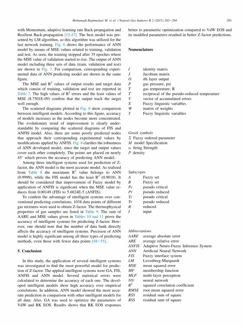
Nomenclature

I identity matrixJ Jacobian matrixO ith layer outputP gas pressure, psiT gas temperature, RT reciprocal of the pseudo-reduced temperatureV vector of accumulated errorsX Fuzzy linguistic variablesW matrix of weightsY Fuzzy linguistic variables

Greek symbols

S Fuzzy ordered parameterМ model Specificationu firing StrengthР density

Subscripts

A Fuzzy setB Fuzzy setPc pseudo criticalPr pseudo reducedTc pseudo criticalTr pseudo reducedR reducedI input

Abbreviations

AARE average absolute errorARE average relative errorANFIS Adaptive Neuro-Fuzzy Inference SystemANN Artificial Neural NetworkFIS Fuzzy interface systemLM Levenberg-MarquardtMSE mean squared errorMF membership functionMLP multi-layer perceptronNN neural networkR2 squared correlation coefficientRMSE root mean squared errorRSS residual sum of squareRSS residual sum of square

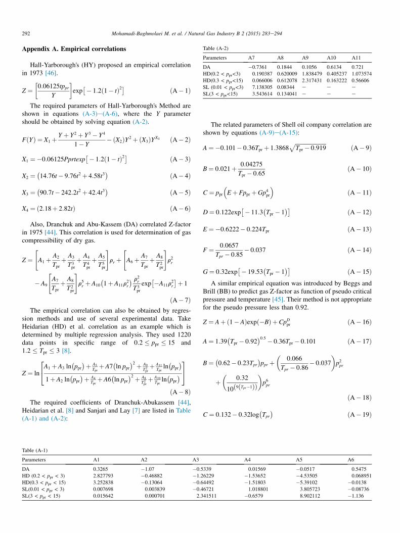
Table (A-2)

Parameters A7 A8 A9 A10 A11

DA �0.7361 0.1844 0.1056 0.6134 0.721

HD(0.2 < ppr<3) 0.190387 0.620009 1.838479 0.405237 1.073574

HD(0.3 < ppr<15) 0.066006 0.612078 2.317431 0.163222 0.56606

SL (0.01 < ppr<3) 7.138305 0.08344 e e eSL(3 < ppr<15) 3.543614 0.134041 e e e

292 Mohamadi-Baghmolaei M. et al. / Natural Gas Industry B 2 (2015) 283e294

Appendix A. Empirical correlations

Hall-Yarborough's (HY) proposed an empirical correlationin 1973 [46].

Z ¼�0:06125tppr

Y

exp� 1:2ð1� tÞ2� ðA� 1Þ

The required parameters of Hall-Yarborough's Method areshown in equations (A-3)e(A-6), where the Y parametershould be obtained by solving equation (A-2).

FðYÞ ¼ X1 þ Y þ Y2 þ Y3 � Y4

1� Y� ðX2ÞY2 þ ðX3ÞYX4 ðA� 2Þ

X1 ¼�0:06125Pprtexp� 1:2ð1� tÞ2� ðA� 3Þ

X2 ¼�14:76t� 9:76t2 þ 4:58t3

� ðA� 4Þ

X3 ¼�90:7t� 242:2t2 þ 42:4t3

� ðA� 5Þ

X4 ¼ ð2:18þ 2:82tÞ ðA� 6Þ

Also, Dranchuk and Abu-Kassem (DA) correlated Z-factorin 1975 [44]. This correlation is used for determination of gascompressibility of dry gas.

Z ¼"A1 þ A2

Tpr

þ A3

T3pr

þ A4

T4pr

þ A5

T5pr

#rr þ

"A6 þ A7

Tpr

þ A8

T2pr

#r2r

�A9

"A7

Tpr

þ A8

T2pr

#r5r þA10

�1þA11r

2r

� r2rT3pr

exp�A11r

2r

�þ 1

ðA� 7ÞThe empirical correlation can also be obtained by regres-

sion methods and use of several experimental data. TakeHeidarian (HD) et al. correlation as an example which isdetermined by multiple regression analysis. They used 1220data points in specific range of 0:2 � ppr � 15 and1:2 � Tpr � 3 [8].

Z ¼ ln

24A1 þA3 ln

�ppr�þ A5

TprþA7

�ln ppr

�2 þ A9

T2prþ A11

Tprln�ppr�

1þA2 ln�ppr�þ A4

TprþA6

�ln ppr

�2 þ A8

T2prþ A10

Tprln�ppr�35

ðA� 8ÞThe required coefficients of Dranchuk-Abukassem [44],

Heidarian et al. [8] and Sanjari and Lay [7] are listed in Table(A-1) and (A-2):

Table (A-1)

Parameters A1 A2 A3

DA 0.3265 �1.07 �0.5

HD (0.2 < ppr < 3) 2.827793 �0.46882 �1.2

HD(0.3 < ppr < 15) 3.252838 �0.13064 �0.6

SL(0.01 < ppr < 3) 0.007698 0.003839 �0.4

SL(3 < ppr < 15) 0.015642 0.000701 2.3

The related parameters of Shell oil company correlation areshown by equations (A-9)e(A-15):

A¼�0:101� 0:36Tpr þ 1:3868ffiffiffiffiffiffiffiffiffiffiffiffiffiffiffiffiffiffiffiffiffiffiTpr � 0:919

p ðA� 9Þ

B¼ 0:021þ 0:04275

Tpr � 0:65ðA� 10Þ

C ¼ ppr

�EþFppr þGp4pr

�ðA� 11Þ

D¼ 0:122exp� 11:3

�Tpr � 1

�� ðA� 12Þ

E ¼�0:6222� 0:224Tpr ðA� 13Þ

F ¼ 0:0657

Tpr � 0:85� 0:037 ðA� 14Þ

G¼ 0:32exp� 19:53

�Tpr � 1

�� ðA� 15ÞA similar empirical equation was introduced by Beggs and

Brill (BB) to predict gas Z-factor as function of pseudo criticalpressure and temperature [45]. Their method is not appropriatefor the pseudo pressure less than 0.92.

Z ¼ Aþ ð1�AÞexpð�BÞ þCpDpr ðA� 16Þ

A¼ 1:39�Tpr � 0:92

�0:5 � 0:36Tpr � 0:101 ðA� 17Þ

B¼ �0:62� 0:23Tpr

�ppr þ

�0:066

Tpr � 0:86� 0:037

�p2pr

þ�

0:32

10ð9ðTpr�1ÞÞ�p6pr

ðA� 18Þ

C ¼ 0:132� 0:32log�Tpr

� ðA� 19Þ

A4 A5 A6

339 0.01569 �0.0517 0.5475

6229 �1.53652 �4.53505 0.068951

4492 �1.51803 �5.39102 �0.0138

6721 1.018801 3.805723 �0.08736

41511 �0.6579 8.902112 �1.136

293Mohamadi-Baghmolaei M. et al. / Natural Gas Industry B 2 (2015) 283e294

D¼ 10ð0:3106�0:49Tprþ0:1824T2prÞ ðA� 20Þ

Papay (PP) proposed simple correlation for estimation ofgas compressibility factor [43]. The correlation was adopted asa function of pseudo reduced pressure and temperature.

Z ¼ 1� 3:53ppr100:9813Tpr

þ 0:274p2pr100:8157Tpr

ðA� 21Þ

Appendix B. Types of errors

Coefficient of determination

R2 ¼ 1�PN

i¼1

�ZPredi � Zexp

i

�2PNi¼1

�ZPredi � averageðZexp

i Þ�2 ðB� 1Þ

Average relative error

ARE%¼ 100

N

XNi¼1

�ZPredi � Zexp

i

Zexpi

�ðB� 2Þ

Average absolute relative error

AARE%¼ 100

N

XNi¼1

� ZPredi � Zexp

i

Zexpi

�

ðB� 3Þ

Root mean square error

RMSE ¼ PN

i¼1

�ZPredi � Zexp

i

�2N

!12

ðB� 4Þ

Residual sum of square

RSS¼XNi¼1

�ZPredi � Zexp

i

�2 ðB� 5Þ

Mean squared error

MSE ¼ 1

N

XNi¼1

�ZPredi � Zexp

i

�2 ðB� 6Þ

References

[1] Ahmed T, McKinney P. Advanced reservoir engineering. Gulf Profes-

sional Publishing; 2011.

[2] Danesh A. PVT and phase behaviour of petroleum reservoir fluids, vol.

47. Elsevier; 1998.

[3] Joffe J, Schroeder GM, Zudkevitch D. Vapor-liquid equilibria with the

redlich-kwong equation of state. AIChE J 1970;16(3):496e8.[4] Abu-Eishah S. Prediction of critical properties of mixtures from the

PRSV-2 equation of state: a correction for predicted critical volumes.

IJOT 1999;20(5):1557e74.

[5] Karimi H, Yousefi F, Papari MM. Prediction of volumetric properties

(pvT) of natural gas mixtures using extended Tao-Mason equation of

state. Chin J Chem Eng 2011;19(3):496e503.

[6] Pedersen KS, Thomassen P, Fredenslund A. Thermodynamics of petro-

leum mixtures containing heavy hydrocarbons. 2. Flash and PVT cal-

culations with the SRK equation of state. Ind Eng Chem Process Des Dev

1984;23(3):566e73.

[7] Sanjari E, Lay EN. An accurate empirical correlation for predicting

natural gas compressibility factors. J Nat Gas Chem Satter

2012;21(2):184e8.

[8] Heidaryan E, Moghadasi J, Rahimi M. New correlations to predict nat-

ural gas viscosity and compressibility factor. J Pet Sci Technol

2010;73(1):67e72.

[9] Azizi N, Behbahani R, Isazadeh M. An efficient correlation for calcu-

lating compressibility factor of natural gases. J Nat Gas Chem Satter

2010;19(6):642e5.

[10] Standing MB, Katz DL. Density of natural gases. Trans AIME

1942;146(01):140e9.

[11] Farzaneh-Gord M, Rahbari H. Developing novel correlations for calcu-

lating natural gas thermodynamic properties. Chem Process Eng

2011;32(4):435e52.

[12] Jarrahian A, Heidaryan E. A new cubic equation of state for sweet and

sour natural gases even when composition is unknown. Fuel

2014;134:333e42.

[13] Mohamadi-Baghmolaei M, Tabkhi F, Sargolzaei J. Exergetic approach to

investigate the arrangement of compressors of a pipeline boosting station.

Energy Technol 2014;2(8):732e41.

[14] Esen H, Inalli M. Modelling of a vertical ground coupled heat pump

system by using artificial neural networks. Expert Syst Appl

2009;36(7):10229e38.[15] MohamadiBaghmolaei M, Mahmoudy M, Jafari D,

MohamadiBaghmolaei R, Tabkhi F. Assessing and optimization of

pipeline system performance using intelligent systems. J Nat Gas Sci Eng

2014;18:64e76.[16] Ahmadi MA, Soleimani R, Bahadori A. A computational intelligence

scheme for prediction equilibrium water dew point of natural gas in TEG

dehydration systems. Fuel 2014;137:145e54.[17] Saemi M, Ahmadi M, Varjani AY. Design of neural networks using ge-

netic algorithm for the permeability estimation of the reservoir. J Pet Sci

Technol 2007;59(1):97e105.

[18] Shojaei M-J, Bahrami E, Barati P, Riahi S. Adaptive neuro-fuzzy

approach for reservoir oil bubble point pressure estimation. J Nat

Gas Sci Eng 2014;20:214e20.

[19] Shokrollahi A, Arabloo M, Gharagheizi F, Mohammadi AH. Intelligent

model for prediction of CO2ereservoir oil minimum miscibility pressure.

Fuel 2013;112:375e84.

[20] Ahmadi MA, Ebadi M. Evolving smart approach for determination dew

point pressure through condensate gas reservoirs. Fuel

2014;117:1074e84.

[21] Sanjari E, Lay EN. Estimation of natural gas compressibility factors using

artificial neural network approach. J Nat Gas Sci Eng 2012;9:220e6.

[22] Kamari A, Hemmati-Sarapardeh A, Mirabbasi S-M, Nikookar M,

Mohammadi AH. Prediction of sour gas compressibility factor using an

intelligent approach. Fuel Process Technol 2013;116:209e16.

[23] Ahmadi MA, Ebadi M, Marghmaleki PS, Fouladi MM. Evolving pre-

dictive model to determine condensate-to-gas ratio in retrograded

condensate gas reservoirs. Fuel 2014;124:241e57.

[24] Ganji-Azad E, Rafiee-Taghanaki S, Rezaei H, Arabloo M, Zamani HA.

Reservoir fluid PVT properties modeling using Adaptive Neuro-Fuzzy

Inference Systems. J Nat Gas Sci Eng 2014;21:951e61.[25] Fayazi A, Arabloo M, Mohammadi AH. Efficient estimation of natural

gas compressibility factor using a rigorous method. J Nat Gas Sci Eng

2014;16:8e17.[26] Rafiee-Taghanaki S, Arabloo M, Chamkalani A, Amani M, Zargari MH,

Adelzadeh MR. Implementation of SVM framework to estimate PVT

properties of reservoir oil. Fluid Phase Equilib 2013;346:25e32.

[27] Chamkalani A, Mae'soumi A, Sameni A. An intelligent approach for

optimal prediction of gas deviation factor using particle swarm optimi-

zation and genetic algorithm. J Nat Gas Sci Eng 2013;14:132e43.

[28] Kumar N. Compressibility factors for natural and sour reservoir gases by

correlations and cubic equations of state. 2004.

[29] Valderrama JO, Silva A. Modified Soave-Redlich-Kwong equations of

state applied to mixtures containing supercritical carbon dioxide. Korean

J Chem Eng 2003;20(4):709e15.

294 Mohamadi-Baghmolaei M. et al. / Natural Gas Industry B 2 (2015) 283e294

[30] Van der Waals JD. Over de Continuiteit van den Gas-en Vloeistoftoe-

stand. AW Sijthoff; 1873.

[31] Redlich O, Kwong J. On the thermodynamics of solutions. V. An

equation of state. Fugacities of gaseous solutions. Chem Rev

1949;44(1):233e44.[32] Soave G. Equilibrium constants from a modified Redlich-Kwong equa-

tion of state. Chem Eng Sci 1972;27(6):1197e203.

[33] Peng D-Y, Robinson DB. A new two-constant equation of state. Ind Eng

Chem Fundam 1976;15(1):59e64.

[34] Yilmaz I, Kaynar O. Multiple regression, ANN (RBF, MLP) and ANFIS

models for prediction of swell potential of clayey soils. Expert Syst Appl

2011;38(5):5958e66.[35] Hornik K, Stinchcombe M, White H. Multilayer feed forward networks

are universal approximators. Neural Netw 1989;2(5):359e66.

[36] Cho I-H, Zoh K-D. Photocatalytic degradation of azo dye (Reactive Red

120) in TiO 2/UV system: optimization and modeling using a response

surface methodology (RSM) based on the central composite design. Dyes

Pigments 2007;75(3):533e43.

[37] Cigizoglu HK. Application of generalized regression neural networks to

intermittent flow forecasting and estimation. J Hydrol Eng

2005;10(4):336e41.

[38] Tanasa DE, Piuleac CG, Curteanu S, Popovici E. Photodegradation

process of Eosin Y using ZnO/SnO2 nanocomposites as photocatalysts:

experimental study and neural network modeling. J Mater Sci

2013;48(22):8029e40.

[39] Jang J-S. ANFIS: adaptive-network-based fuzzy inference system. Sys-

tems, Man and Cybernetics, IEEE Trans 1993;23(3):665e85.[40] Shoorehdeli MA, Teshnehlab M, Sedigh AK. Training ANFIS as an

identifier with intelligent hybrid stable learning algorithm based on

particle swarm optimization and extended Kalman filter. Fuzzy Sets Syst

2009;160(7):922e48.

[41] Darwin C, Bynum WF. The origin of species by means of natural se-

lection: or, the preservation of favored races in the struggle for life. AL

Burt; 2009.

[42] Holland JH. Adaptation in natural and artificial systems: an introductory

analysis with applications to biology, control, and artificial intelligence.

U Michigan Press; 1975.

[43] Papay J. A Termelestechnologiai Parameterek Valtozasa a gazlelepk

muvelese Soran. OGIL MUSZ Tud Kuzl 1968:267e73. Budapest.

[44] Dranchuk P, Kassem H. Calculation of Z factors for natural gases using

equations of state. 1975.

[45] Beggs DH, Brill JP. A study of two-phase flow in inclined pipes. J Petrol

Technol 1973;25(05):607e17.

[46] Hall K, Yarborough L. A new EOS for z-factor calculations. Oil Gas J

1973:82.

[47] Toma F-L, Guessasma S, Klein D, Montavon G, Bertrand G, Coddet C.

Neural computation to predict TiO2 photocatalytic efficiency for nitrogen

oxides removal. J Photochem Photobiol A 2004;165(1):91e6.

[48] Li Q, Guo T-M. A study on the supercompressibility and compressibility

factors of natural gas mixtures. J Pet Sci Technol 1991;6(3):235e47.

[49] Buxton TS, Campbell JM. Compressibility factors for lean natural gas-

carbon dioxide mixtures at high pressure. Soc Petrol Eng J

1967;7(1):80e6.[50] Sun C-Y, Liu H, Yan K-L, Ma Q-L, Liu B, Chen G-J, et al. Experiments

and modeling of volumetric properties and phase behavior for condensate

gas under ultra-high-pressure conditions. Ind Eng Chem Res

2012;51(19):6916e25.

[51] �Capla L, Buryan P, Jedelsky J, Rottner M, Linek J. Isothermal pVT

measurements on gas hydrocarbon mixtures using a vibrating-tube

apparatus. J Chem Thermodyn 2002;34(5):657e67.[52] Yan K-L, Liu H, Sun C-Y, Ma Q-L, Chen G-J, Shen D-J, et al. Mea-

surement and calculation of gas compressibility factor for condensate gas

and natural gas under pressure up to 116MPa. J Chem Thermodyn

2013;63:38e43.[53] Chamorro C, Segovia J, Martın M, Villama~n�an M, Estela-Uribe J,

Trusler J. Measurement of the (pressure, density, temperature) relation of

two (methaneþ nitrogen) gas mixtures at temperatures between 240 and

400K and pressures up to 20MPa using an accurate single-sinker

densimeter. J Chem Thermodyn 2006;38(7):916e22.

[54] Satter A, Campbell JM. Non-ideal behavior of gases and their mixtures.

Soc Petrol Eng J 1963;3(4):333e47.[55] Hou H, Holste JC, Hall KR, Marsh KN, Gammon BE. Second and third

virial coefficients for methaneþ ethane and methaneþ ethaneþ carbon

dioxide at (300 and 320). K J Chem Eng Data 1996;41(2):344e53.