Embed Size (px)
Citation preview
ENGI N EE RI NG
GOR
and ENVIRONMENTAL ENGINEERING
UP
CO E AN
Bikash Mishra
August 2005
Report No. 05−1
ENVIRONMENTAL AND WATER RESOURCES ENGINEERING
Austin, TX 78712
DEPARTMENT OF CIVIL, ARCHITECTURAL
Prediction of Performance of Podded Propulsors
via Coupling of a Vortex−Lattice Method
with an Euler or a RANS Solver
THE UNIVERSITY OF TEXAS AT AUSTIN

Copyright
by
Bikash Mishra
2005

Prediction of Performance of Podded Propulsors via Coupling ofa Vortex-Lattice Method with an Euler or a RANS solver
by
Bikash Mishra, B.Tech.
Thesis
Presented to the Faculty of the Graduate School
of The University of Texas at Austin
in Partial Fulfillment
of the Requirements
for the Degree of
Master of Science in Engineering
The University of Texas at Austin
August 2005
Prediction of Performance of Podded Propulsors via Coupling ofa Vortex-Lattice Method with an Euler or a RANS solver
APPROVED BYSUPERVISING COMMITTEE:
Supervisor:Spyros A. Kinnas
Reader:Loukas Kallivokas

To my parents, brother and friends

Acknowledgements
I would like to take this opportunity to thank several people whose support, guidance
and encouragement egged me on during my research work and helped me complete
my Masters thesis.
First and foremost, I would like to thank my supervisor, Dr. Spyros A. Kin-
nas with greatest appreciation and gratefulness. His guidance and insights were of
immense help during the course of my studies and research.
I would also like to thank Dr. Loukas F. Kallivokas for taking his time out
of his busy schedule and reading this thesis, and providing me with invaluable com-
ments, assistance and encouragement.
I would like to thank my parents, my brother Bivas and my friends, especially
Piyush, Sanketh and Aswin who stood by me throughout this process and picked me
up with their encouraging words every time I faltered.
I would like to thank the members of the Computational Hydrodynamics
Laboratory, Dr. Hanseong Lee, Mr. Hua Gu, Mr. Bharani Kacham, Mr.Apurva
Gupta, Mr. Yi-Hsiang Yu, Ms. Hong Sun,, Mr. Vimal Vinayan, Mr. Yumin Deng,
Mr. Fahad Mohammad and Mr. Lei He for their unending support and suggestions.
I would also like to thank Dr. Rhee of FLUENT Inc. for the invaluable suggestions
he provided regarding FLUENT.
Support for this research was provided by Phase III, and IV of the “Con-
v

sortium on Cavitation Performance of High Speed Propulsors” with the following
members: AB Volvo Penta, American Bureau of Shipping, Daewoo Shipbuilding
and Marine Engineering Co. Ltd., El Pardo Model Basin, Hyundai Maritime Re-
search Institute, Kawasaki Heavy Industries, Naval Surface Warfare Center Carde-
rock Division through the Office of Naval Research (Contracts N00014-01-1-0225
and N00014-04-1-0287), Rolls-Royce marine AB, Rolls-Royce Marine AS, VA
Tech Escher Wyss GMBH, Wartsila Propulsion Netherlands B.V., and Wartsila
Propulsion Norway AS. Partial support of this work was also provided by the Office
of Naval Research under the National Naval Responsibility for Naval Engineering
(NNR-NE) program, through Florida Atlantic University (Subagreement TRD67).
Finally I would like to thank the faculty of the College of Engineering at theUniversity of Texas at Austin for the excellent education they provided.
vi

Prediction of Performance of Podded Propulsors via Coupling of a
Vortex-Lattice Method with an Euler or a RANS solver
by
Bikash Mishra, M.S.E.
The University of Texas at Austin, 2005
SUPERVISOR: Spyros A. Kinnas
Podded propulsor units are one of the latest innovations in the field of
propulsion, and are used in many commercial or naval vessels. The major advantage
of these units over conventional propeller based systems is their ability to provide
thrust in all directions, giving high maneuverability and good seakeeping character-
istics.
In this work podded propulsors are modeled using axi-symmetric (assuming
an axisymmetric pod and ignoring the presence of strut) or 3-D solvers. At first,
a Vortex Lattice Method (MPUF-3A) is coupled with an Euler solver (GBFLOW-
3X/3D). MPUF-3A is used to solve for the potential flow around each propeller,
obtain the pressure distribution on the blades and predict the thrust and torque for
each propeller. The pressure distributions are then converted into body forces which
represent the propeller in GBFLOW. GBFLOW solves for the flow around the pod
vii
(and strut) and the effective wake to each propeller is calculated. Iterations are
carried out between the two methods till convergence is obtained, and the complete
interaction among each one of the propellers (in the case of a twin propeller system)
and the pod (and strut) is captured.
The same procedure is then applied by coupling the commercial code FLU-
ENT with MPUF-3A. This coupling is used to predict the effects of viscosity on the
flow field and on the overall podded propeller performance.
The objective of this research is to predict the forces on the podded unit in
inviscid and viscous flow field and to compare the results from the two approaches
with each other and with measurements from experiments.
viii

Table of Contents
Acknowledgements v
Abstract vii
List of Tables iv
List of Figures vi
Nomenclature xiii
Chapter 1. Introduction 11.1 Background . . . . . . . . . . . . . . . . . . . . . . . . . . . . . . 1
1.2 Motivation . . . . . . . . . . . . . . . . . . . . . . . . . . . . . . . 5
1.3 Objectives . . . . . . . . . . . . . . . . . . . . . . . . . . . . . . . 7
1.4 Overview . . . . . . . . . . . . . . . . . . . . . . . . . . . . . . . . 8
Chapter 2. Literature Review 102.1 Vortex Lattice Method . . . . . . . . . . . . . . . . . . . . . . . . . 10
2.2 Effective Wake Prediction . . . . . . . . . . . . . . . . . . . . . . . 11
2.2.1 Multi-Component Propulsors . . . . . . . . . . . . . . . . . 12
2.2.2 Podded Propulsors . . . . . . . . . . . . . . . . . . . . . . . 14
Chapter 3. Formulation and Numerical Implementation 173.1 Continuity and Euler Equations . . . . . . . . . . . . . . . . . . . . 17
3.2 Steady Euler Solver . . . . . . . . . . . . . . . . . . . . . . . . . . 18
3.2.1 Axisymmetric Steady Euler Solver . . . . . . . . . . . . . . 19
3.2.2 Three-dimensional Steady Euler-Solver . . . . . . . . . . . . 20
3.2.3 Boundary Conditions . . . . . . . . . . . . . . . . . . . . . . 22
3.3 Vortex Lattice Method . . . . . . . . . . . . . . . . . . . . . . . . . 29
3.4 Boundary Element Method . . . . . . . . . . . . . . . . . . . . . . 30
i

3.4.1 Formulation of Potential Flow around a Pod and Strut . . . . 31
3.4.2 Kinematic Boundary Condition on the Body . . . . . . . . . 32
3.4.3 Kutta Condition . . . . . . . . . . . . . . . . . . . . . . . . 32
3.4.4 Hull Effects . . . . . . . . . . . . . . . . . . . . . . . . . . . 33
3.5 FLUENT . . . . . . . . . . . . . . . . . . . . . . . . . . . . . . . . 33
3.6 Coupling to determine pod and propeller interaction . . . . . . . . . 35
3.6.1 GBFLOW or FLUENT/MPUF-3A coupling . . . . . . . . . 35
3.6.2 Coupling of Non-dimensional Forces from FVM and VLM . 37
3.6.3 BEM/MPUF3A coupling . . . . . . . . . . . . . . . . . . . 39
Chapter 4. Validation and Comparisons with Other Methods - Axisym-metric Pod 42
4.1 Axisymmetric Euler Solver . . . . . . . . . . . . . . . . . . . . . . 42
4.1.1 Grid and Boundary Conditions . . . . . . . . . . . . . . . . 43
4.1.2 Results . . . . . . . . . . . . . . . . . . . . . . . . . . . . . 45
4.2 FLUENT . . . . . . . . . . . . . . . . . . . . . . . . . . . . . . . . 47
4.2.1 Grid and Boundary Conditions . . . . . . . . . . . . . . . . 48
4.2.2 Results . . . . . . . . . . . . . . . . . . . . . . . . . . . . . 52
4.2.3 Viscous effects . . . . . . . . . . . . . . . . . . . . . . . . . 54
4.2.4 Study of different models . . . . . . . . . . . . . . . . . . . 63
4.3 BEM . . . . . . . . . . . . . . . . . . . . . . . . . . . . . . . . . . 65
4.3.1 Results . . . . . . . . . . . . . . . . . . . . . . . . . . . . . 66
4.4 Comparisons among different methods . . . . . . . . . . . . . . . . 69
Chapter 5. Axisymmetric Pod and Propeller Interaction 725.1 Experiment . . . . . . . . . . . . . . . . . . . . . . . . . . . . . . . 72
5.1.1 Experimental Setup . . . . . . . . . . . . . . . . . . . . . . 73
5.2 Propeller Configurations . . . . . . . . . . . . . . . . . . . . . . . . 74
5.3 Pull Type . . . . . . . . . . . . . . . . . . . . . . . . . . . . . . . . 75
5.3.1 Coupling with GBFLOW-3X . . . . . . . . . . . . . . . . . 75
5.3.2 Coupling with FLUENT . . . . . . . . . . . . . . . . . . . . 81
5.4 Push Type . . . . . . . . . . . . . . . . . . . . . . . . . . . . . . . 97
5.4.1 Coupling with GBFLOW-3X . . . . . . . . . . . . . . . . . 97
5.4.2 Coupling with FLUENT . . . . . . . . . . . . . . . . . . . . 101
ii
5.5 Twin type . . . . . . . . . . . . . . . . . . . . . . . . . . . . . . . 113
5.5.1 Coupling of GBFLOW-3X . . . . . . . . . . . . . . . . . . . 113
5.5.2 Coupling with FLUENT . . . . . . . . . . . . . . . . . . . . 117
Chapter 6. Pod with strut 1266.1 3-D Euler Solver (GBFLOW-3D) . . . . . . . . . . . . . . . . . . . 126
6.1.1 Grid Generation . . . . . . . . . . . . . . . . . . . . . . . . 127
6.1.2 Boundary Conditions . . . . . . . . . . . . . . . . . . . . . . 129
6.1.3 Results . . . . . . . . . . . . . . . . . . . . . . . . . . . . . 129
6.2 FLUENT-3D . . . . . . . . . . . . . . . . . . . . . . . . . . . . . . 133
6.2.1 Grid and boundary conditions . . . . . . . . . . . . . . . . . 135
6.2.2 Inviscid Results . . . . . . . . . . . . . . . . . . . . . . . . 138
6.2.3 Viscous Results . . . . . . . . . . . . . . . . . . . . . . . . 138
6.3 Comparison among different methods . . . . . . . . . . . . . . . . . 142
Chapter 7. Conclusions and Recommendations 1477.1 Conclusions . . . . . . . . . . . . . . . . . . . . . . . . . . . . . . 147
7.2 Recommendations . . . . . . . . . . . . . . . . . . . . . . . . . . . 148
Appendix A 149
Bibliography 159
Vita 169
iii

List of Tables
4.1 Total force on the pod from Euler solver for axisymmetric runs fordifferent grid densities. Forces made non-dimensional as given byequation 3.5 . . . . . . . . . . . . . . . . . . . . . . . . . . . . . . 46
4.2 Run parameters for the 2-D axisymmetric inviscid version of FLUENT 51
4.3 Total force on the pod and the computed surface area from FLUENTfor axisymmetric runs for different grid densities. . . . . . . . . . . 56
4.4 Run parameters for 2-D axisymmetric viscous FLUENT . . . . . . 56
4.5 Reynolds number, k and ε for which runs are carried out using vis-cous FLUENT . . . . . . . . . . . . . . . . . . . . . . . . . . . . . 61
4.6 Comparison of mean empirical frictional force coefficient Cf withthat from k − ε model . . . . . . . . . . . . . . . . . . . . . . . . . 63
4.7 Total force on the pod from BEM for axisymmetric runs for differentpaneling. . . . . . . . . . . . . . . . . . . . . . . . . . . . . . . . . 68
5.1 Break-up of forces from MPUF-3A and GBFLOW-3X for pullingpropeller for various advance ratios . . . . . . . . . . . . . . . . . . 81
5.2 Break-up of forces from MPUF-3A and FLUENT for pulling pro-peller for various advance ratios . . . . . . . . . . . . . . . . . . . 85
5.3 Break-up of forces from MPUF-3A and viscous FLUENT for pullingpropeller for various advance ratios . . . . . . . . . . . . . . . . . . 90
5.4 Break-up of forces from MPUF-3A and GBFLOW-3X for pushingpropeller for various advance ratios . . . . . . . . . . . . . . . . . . 100
5.5 Break-up of forces from MPUF-3A and inviscid FLUENT for push-ing propeller for various advance ratios . . . . . . . . . . . . . . . . 103
5.6 Break-up of forces from MPUF-3A and viscous FLUENT for push-ing propeller for various advance ratios . . . . . . . . . . . . . . . . 109
5.7 Break-up of forces from MPUF-3A and GBFLOW-3X for twin pro-peller unit for various advance ratios . . . . . . . . . . . . . . . . . 115
5.8 Break-up of forces from MPUF-3A and FLUENT (RSM) for twinpropeller unit for various advance ratios . . . . . . . . . . . . . . . 119
6.1 Run parameters for 3-D viscous FLUENT . . . . . . . . . . . . . . 139
iv

1 The pod geometry used by [Szantyr 2001a] . . . . . . . . . . . . . 151
2 The parabolic section strut used for GBFLOW-3D runs with leadingedge at the location X=-0.6 on the pod, and trailing edge at X=+0.6 . 152
3 The strut used by [Szantyr 2001a] for the experimental measure-ments. It is a NACA066 section, and has the leading edge at thelocation X=-0.6 on the pod, and trailing edge at X=+0.6 . . . . . . . 153
4 Front propeller geometry. The front propeller placed at the location-1.1899 on the pod . . . . . . . . . . . . . . . . . . . . . . . . . . 154
5 The specific stations along the chord where the propeller blade thick-ness and camber distributions are specified, at the given radii locations.155
6 The camber distribution specified at the nine radii locations specifiedin the geometry file and at specific stations along the chord. . . . . . 156
7 The thickness distribution specified at the nine radii locations spec-ified in the geometry file and at specific stations along the chord. . . 157
8 Geometry of the aft propeller. The aft propeller placed at the loca-tion 1.1899 on the pod. The thickness and camber distributions arethe same as for the fore propeller. . . . . . . . . . . . . . . . . . . . 158
v

List of Figures
1.1 Figure showing a pull type podded unit. . . . . . . . . . . . . . . . 21.2 Figure showing a push type podded unit. . . . . . . . . . . . . . . . 3
1.3 Figure showing a twin type podded unit. . . . . . . . . . . . . . . . 4
3.1 Ship-fixed Cartesian coordinate system (taken from [Choi 2000]) . . 19
3.2 2-D grid showing the boundary conditions used for the axisymmetricEuler solver . . . . . . . . . . . . . . . . . . . . . . . . . . . . . . 22
3.3 Boundary conditions for the Euler solver which evaluates the flowaround the pod and strut in the presence of the propeller, (taken from[Gupta 2004]). . . . . . . . . . . . . . . . . . . . . . . . . . . . . . 25
3.4 Boundary conditions on the domain at an axial location showing podand strut (no repeat boundary), (taken from [Gupta 2004]) . . . . . 26
3.5 Boundary conditions on the domain at an axial location showing therepeat boundary (k = 1, Nk), (taken from [Gupta 2004]) . . . . . . 27
3.6 Pictorial representation of the coupling of the Finite Volume Methodand the Vortex Lattice Method (from [Kinnas, Gu, Gupta and Lee2004]). . . . . . . . . . . . . . . . . . . . . . . . . . . . . . . . . . 36
3.7 Pictorial representation of the coupling of the Boundary ElementMethod and the Vortex Lattice Method. . . . . . . . . . . . . . . . 41
4.1 2-D grid showing the boundaries for the axisymmetric Euler solver . 444.2 Closeup of the leading and trailing edge showing the uniform ex-
pansion ratio. . . . . . . . . . . . . . . . . . . . . . . . . . . . . . 44
4.3 Close-up of different grids (near the leading edge) used for conver-gence studies in GBFLOW-3X without propeller . . . . . . . . . . 46
4.4 Convergence of axial velocities on body with different grids in GBFLOW-3X (number of nodes in axial direction is varied) . . . . . . . . . . 47
4.5 Convergence of pressure on body with different grids in GBFLOW-3X (number of nodes in axial direction is varied) . . . . . . . . . . 48
4.6 Axial velocity contour around the body from GBFLOW-3X . . . . . 494.7 Pressure contour around the body from GBFLOW-3X . . . . . . . . 50
4.8 Unstructured grid used in inviscid FLUENT showing the inflow andoutflow boundaries. . . . . . . . . . . . . . . . . . . . . . . . . . . 51
vi

4.9 Unstructured grid used in viscous FLUENT showing the inflow andoutflow boundaries. . . . . . . . . . . . . . . . . . . . . . . . . . . 52
4.10 A closeup view of the grid near the pod, showing the boundary layerused and the triangular grid at the leading edge of the pod. . . . . . 53
4.11 Structured grid used in FLUENT and exported from GBFLOW-3X . 53
4.12 Convergence of axial velocities on body with different unstructuredgrids using FLUENT (inviscid) . . . . . . . . . . . . . . . . . . . . 54
4.13 Convergence of pressure on body with different unstructured gridsusing FLUENT (inviscid) . . . . . . . . . . . . . . . . . . . . . . . 55
4.14 Axial velocity contour and streamlines from inviscid FLUENT . . . 57
4.15 Pressure contour from inviscid FLUENT . . . . . . . . . . . . . . . 58
4.16 Axial velocities on body with unstructured and structured grids (FLU-ENT inviscid) as shown in Figures 4.8 and 4.11 . . . . . . . . . . . 59
4.17 Pressure on body with unstructured and structured grids (FLUENTinviscid) as shown in Figures 4.8 and 4.11 . . . . . . . . . . . . . . 59
4.18 Axial velocities near leading edge with unstructured and structuredgrids at location shown in Figure 4.19 . . . . . . . . . . . . . . . . 60
4.19 Locations where inviscid FLUENT and GBFLOW-3X axial veloci-ties are compared . . . . . . . . . . . . . . . . . . . . . . . . . . . 60
4.20 Comparison of axial velocities for inviscid FLUENT and GBFLOW-3X at given location . . . . . . . . . . . . . . . . . . . . . . . . . . 61
4.21 Comparison of pressure for inviscid FLUENT and GBFLOW-3X atgiven location . . . . . . . . . . . . . . . . . . . . . . . . . . . . . 62
4.22 Y + on the pod for viscous FLUENT run, Re=4.5 × 10⁵ . . . . . . . 62
4.23 Locations for comparison of inviscid and viscous axial velocities . . 64
4.24 Axial velocities for different Re at Xf=-0.415 location as shown inFigure 4.23. . . . . . . . . . . . . . . . . . . . . . . . . . . . . . . 64
4.25 Axial velocities from different methods at Xa=1.93 location as shownin Figure 4.23, Re = 6.26 × 10⁵. . . . . . . . . . . . . . . . . . . . 65
4.26 Grid used for the axisymmetric BEM solver . . . . . . . . . . . . . 66
4.27 Convergence of axial velocities with different grids using BEM . . . 67
4.28 Convergence of pressure with different grids using BEM . . . . . . 67
4.29 Convergence of forces with number of cells from all methods . . . . 68
4.30 Non-dimensional axial velocity on the pod from axisymmetric in-viscid FLUENT and BEM compared with GBFLOW-3X. . . . . . . 70
4.31 Non dimensional pressure on the pod from axisymmetric inviscidFLUENT and BEM compared with GBFLOW-3X. . . . . . . . . . 71
vii

5.1 Axial body force contours in GBLFOW-3X domain obtained by in-tegration of pressures on the propeller, for a pull type podded propul-sor, Js = 0.5. . . . . . . . . . . . . . . . . . . . . . . . . . . . . . 76
5.2 Close-up of axial body force contours in GBLFOW-3X for a pulltype podded propulsor, Js = 0.5. . . . . . . . . . . . . . . . . . . . 76
5.3 Axial velocity contour in GBFLOW-3X for pull type podded propul-sor, Js = 0.5 . . . . . . . . . . . . . . . . . . . . . . . . . . . . . . 77
5.4 Pressure contour in GBFLOW-3X for pull type podded propulsor,Js = 0.5 . . . . . . . . . . . . . . . . . . . . . . . . . . . . . . . . 77
5.5 Convergence of circulation distribution with iterations for GBFLOW-3X coupled with MPUF-3A, for pull type podded propulsor, Js = 0.5 78
5.6 Pictorial representation of the direction of forces from MPUF-3Aand GBFLOW/FLUENT, for 00 yaw angle. . . . . . . . . . . . . . 79
5.7 Comparison of axial force for a pulling propeller from the presentmethod compared with the measurements of [Szantyr 2001a]. . . . 80
5.8 Axial body force distribution in FLUENT for an unstructured grid,Js = 0.5 . . . . . . . . . . . . . . . . . . . . . . . . . . . . . . . . 82
5.9 Axial body force distribution in FLUENT for a structured grid, Js =0.5 . . . . . . . . . . . . . . . . . . . . . . . . . . . . . . . . . . . 82
5.10 Convergence of axial body force distribution in FLUENT for vary-ing grid sizes, Js = 0.5 . . . . . . . . . . . . . . . . . . . . . . . . 83
5.11 Axial body force distribution in FLUENT over a very fine structuredgrid, Js = 0.5 . . . . . . . . . . . . . . . . . . . . . . . . . . . . . 84
5.12 Axial velocity contour from inviscid FLUENT for pull type poddedpropulsor, Js = 0.5 . . . . . . . . . . . . . . . . . . . . . . . . . . 85
5.13 Pressure contour from inviscid FLUENT for pull type podded propul-sor, Js = 0.5 . . . . . . . . . . . . . . . . . . . . . . . . . . . . . . 86
5.14 Comparison of converged circulation distributions predicted fromGBFLOW-3X and FLUENT(inviscid) coupled with MPUF-3A, forpull type podded propulsor, Js = 0.5 . . . . . . . . . . . . . . . . . 87
5.15 Comparison of axial force for a pulling propeller from FLUENT(inviscid)and GBFLOW-3X coupled with MPUF-3A. . . . . . . . . . . . . . 88
5.16 Axial velocity contour in viscous FLUENT for pull type poddedpropulsor, Js = 0.5, Re = 6.26 × 10⁵ . . . . . . . . . . . . . . . . 89
5.17 Pressure contour in viscous FLUENT for pull type podded propul-sor, Js = 0.5, Re = 6.26 × 10⁵ . . . . . . . . . . . . . . . . . . . . 90
5.18 Total axial velocity at effective wake location for viscous and invis-cid FLUENT coupled with MPUF-3A, for pull type podded propul-sor, Js = 0.5, Re = 6.26 × 10⁵ . . . . . . . . . . . . . . . . . . . . 91
viii

5.19 Converged circulation distributions predicted from FLUENT (vis-cous) and FLUENT(inviscid) coupled with MPUF-3A, for pull typepodded propulsor, Js = 0.5, Re = 6.26 × 10⁵ . . . . . . . . . . . . 92
5.20 Converged pressure distributions predicted from GBFLOW-3X, FLU-ENT (viscous) and FLUENT(inviscid) coupled with MPUF-3A, forpull type podded propulsor, Js = 0.5, Re = 6.26 × 10⁵ . . . . . . . 93
5.21 Comparison of axial force for a pulling propeller from FLUENT(inviscid& viscous) and GBFLOW coupled with MPUF-3A. . . . . . . . . . 94
5.22 Comparison of axial velocity at aft effective wake location from in-viscid, k − ε and RSM models, Js = 0.5Re = 6.26 × 10⁵. . . . . . 95
5.23 Comparison of swirl velocity at aft effective wake location from in-viscid, k − ε and RSM models, Js = 0.5Re = 6.26 × 10⁵. . . . . . 96
5.24 Body force contours in GBLFOW-3X domain obtained by integra-tion of pressures on the propeller, for a push type podded propulsor,Js = 0.5. . . . . . . . . . . . . . . . . . . . . . . . . . . . . . . . 97
5.25 Axial velocity contour in GBFLOW-3X for push type podded propul-sor, Js = 0.5 . . . . . . . . . . . . . . . . . . . . . . . . . . . . . . 98
5.26 Pressure contour in GBFLOW-3X for push type podded propulsor,Js = 0.5 . . . . . . . . . . . . . . . . . . . . . . . . . . . . . . . . 99
5.27 Convergence of circulation distribution with iterations for GBFLOW-3X for push type podded propulsor, Js = 0.5 . . . . . . . . . . . . 99
5.28 Body force distribution in FLUENT on the grid for inviscid case,Js = 0.5 . . . . . . . . . . . . . . . . . . . . . . . . . . . . . . . . 101
5.29 Body force distribution in FLUENT on the grid for viscous case,Js = 0.5, Re = 6.26 × 10⁵ . . . . . . . . . . . . . . . . . . . . . . 102
5.30 Axial velocity contour in inviscid FLUENT for push type poddedpropulsor, Js = 0.5 . . . . . . . . . . . . . . . . . . . . . . . . . . 103
5.31 Comparison of effective axial velocity between GBFLOW-3X andFLUENT (inviscid) coupled with MPUF-3A, for a push type unit,Js = 0.5. . . . . . . . . . . . . . . . . . . . . . . . . . . . . . . . 104
5.32 Converged circulation distributions predicted from GBFLOW-3Xand FLUENT(inviscid) coupled with MPUF-3A, for push type pod-ded propulsor, Js = 0.5 . . . . . . . . . . . . . . . . . . . . . . . . 105
5.33 Axial force for a pushing propeller predicted from FLUENT (invis-cid) and GBFLOW-3X coupled with MPUF-3A. . . . . . . . . . . . 106
5.34 Axial velocity contours predicted by viscous FLUENT for push typepodded propulsor, Js = 0.5, Re = 6.26 × 10⁵ . . . . . . . . . . . . 107
5.35 Comparison of total axial velocity at effective wake plane locationfrom inviscid and viscous FLUENT coupled with MPUF-3A, Js =0.5, Re = 6.26 × 10⁵ . . . . . . . . . . . . . . . . . . . . . . . . . 108
ix

5.36 Comparison of effective velocity at effective wake plane locationfrom inviscid and viscous FLUENT coupled with MPUF-3A, Js =0.5, Re = 6.26 × 10⁵ . . . . . . . . . . . . . . . . . . . . . . . . . 109
5.37 Comparison of converged circulation from inviscid and viscous FLU-ENT coupled with MPUF-3A, Js = 0.5, Re = 6.26 × 10⁵ . . . . . . 110
5.38 Comparison of pressure distributions along the body for a push-ing propeller from FLUENT(inviscid & viscous) and GBFLOW-3Xcoupled with MPUF-3A. . . . . . . . . . . . . . . . . . . . . . . . 111
5.39 Comparison of axial force for a pushing propeller from FLUENT(inviscid& viscous) and GBFLOW-3X coupled with MPUF-3A. . . . . . . . 112
5.40 Axial velocity contour in GBFLOW-3X for twin type podded propul-sor, Js = 0.5 . . . . . . . . . . . . . . . . . . . . . . . . . . . . . . 114
5.41 Pressure contour in GBFLOW-3X for twin type podded propulsor,Js = 0.5 . . . . . . . . . . . . . . . . . . . . . . . . . . . . . . . . 114
5.42 Convergence of circulation distribution with iterations for fore pro-peller from GBFLOW-3X for twin type podded propulsor, Js = 0.5 115
5.43 Convergence of circulation distribution with iterations for aft pro-peller from GBFLOW-3X for twin type podded propulsor, Js = 0.5 116
5.44 Comparison of axial force for a twin type propeller unit from presentmethod compared with experiments of [Szantyr 2001a]. . . . . . . . 116
5.45 Axial velocity contour from viscous FLUENT for twin type poddedpropulsor, Js = 0.5, Re = 6.26 × 10⁵ . . . . . . . . . . . . . . . . 117
5.46 Pressure contour from viscous FLUENT for twin type podded propul-sor, Js = 0.5, Re = 6.26 × 10⁵ . . . . . . . . . . . . . . . . . . . . 118
5.47 Comparison of effective velocity for fore propeller between GBFLOW-3X and FLUENT (viscous) coupled with MPUF-3A, for a twin typeunit, Js = 0.5, Re = 6.26 × 10⁵. . . . . . . . . . . . . . . . . . . . 119
5.48 Comparison of effective axial velocity for aft propeller predictedfrom GBFLOW-3X and FLUENT (viscous) coupled with MPUF-3A, for a twin type unit, Js = 0.5, Re = 6.26 × 10⁵. . . . . . . . . . 120
5.49 Comparison of effective swirl velocity for aft propeller predictedfrom GBFLOW-3X and FLUENT (viscous) coupled with MPUF-3A, for a twin type unit, Js = 0.5, Re = 6.26 × 10⁵. . . . . . . . . . 121
5.50 Comparison of circulation distributions for fore propeller predictedfrom GBFLOW-3X and FLUENT (viscous) coupled with MPUF-3A, for a twin type unit, Js = 0.5, Re = 6.26 × 10⁵. . . . . . . . . . 122
5.51 Comparison of circulation distributions for aft propeller predictedfrom GBFLOW-3X and FLUENT (viscous) coupled with MPUF-3A, for a twin type unit, Js = 0.5, Re = 6.26 × 10⁵. . . . . . . . . . 123
x

5.52 Comparison of pressure distributions along the body for a twin pro-peller from FLUENT(viscous) and GBFLOW-3X coupled with MPUF-3A. . . . . . . . . . . . . . . . . . . . . . . . . . . . . . . . . . . 124
5.53 Comparison of axial force for a twin type propeller unit from GBFLOW-3X and viscous FLUENT coupled with MPUF-3A. . . . . . . . . . 125
6.1 Cross-sectional view of the domain in axial direction showing thetype of grid cells distribution at different locations (taken from [Gupta2004]). . . . . . . . . . . . . . . . . . . . . . . . . . . . . . . . . . 127
6.2 Cross-sectional view of the domain showing the grid cells near thestrut and the pod. Circumferential cells are uniformly distributed. . . 128
6.3 Cross-sectional view of the domain showing the grid cells near thestrut and the pod. Circumferential cells are clustered near the strut. . 129
6.4 Location on strut where velocity and pressure comparisons are car-ried out. . . . . . . . . . . . . . . . . . . . . . . . . . . . . . . . . 130
6.5 Convergence of axial velocity with varying number of nodes in axialdirection in GBFLOW-3D. . . . . . . . . . . . . . . . . . . . . . . 131
6.6 Convergence of pressure with varying number of nodes in axial di-rection in GBFLOW-3D. . . . . . . . . . . . . . . . . . . . . . . . 131
6.7 Comparison of axial velocity between the two different types ofgrids used in k direction in GBFLOW-3D, k = 121 . . . . . . . . . 132
6.8 Comparison of pressure between the two different types of gridsused in k direction in GBFLOW-3D, k = 121 . . . . . . . . . . . . 132
6.9 Different grids for which convergence with varying number of nodesalong the circumferential direction in GBFLOW-3D . . . . . . . . . 133
6.10 Convergence of axial velocity with varying number of nodes alongthe circumferential direction in GBFLOW-3D . . . . . . . . . . . . 134
6.11 Convergence of pressure with varying number of nodes along thecircumferential direction in GBFLOW-3D . . . . . . . . . . . . . . 134
6.12 The domain used in 3D FLUENT, showing the projection in x-y plane.136
6.13 The domain used in 3D FLUENT, showing the projection in y-z plane.136
6.14 Close up of the grid used in 3D FLUENT near the pod and strut inthe x-y plane. . . . . . . . . . . . . . . . . . . . . . . . . . . . . . 137
6.15 Close up of the grid used in 3D FLUENT near the pod and strut inthe y-z plane. . . . . . . . . . . . . . . . . . . . . . . . . . . . . . 137
6.16 Convergence of axial velocity with varying number of nodes on thepod using FLUENT-3D (inviscid). . . . . . . . . . . . . . . . . . . 138
6.17 Convergence of pressure with varying number of nodes on the podusing FLUENT-3D (inviscid). . . . . . . . . . . . . . . . . . . . . 139
xi

6.18 y+ distribution over the 3D pod and strut. . . . . . . . . . . . . . . 140
6.19 Locations behind the strut where the velocity and pressure compar-isons are carried out for viscous 3D FLUENT. . . . . . . . . . . . . 141
6.20 Convergence of axial velocity with varying number of nodes on thepod using FLUENT-3D (viscous), Re = 4.52 × 10⁶. . . . . . . . . 141
6.21 Convergence of pressure with varying number of nodes on the podusing FLUENT-3D (viscous), Re = 4.52 × 10⁶. . . . . . . . . . . . 142
6.22 Comparison of axial velocity on the pod among the different methods.143
6.23 Comparison of pressure on the pod among the different methods. . . 143
6.24 Comparison of axial velocity among inviscid and viscous 3D FLU-ENT at the line on the x-z plane, Re = 4.52 × 10⁶. . . . . . . . . . 144
6.25 Comparison of pressure among inviscid and viscous 3D FLUENT atthe line on the x-z plane, Re = 4.52 × 10⁶. . . . . . . . . . . . . . . 145
6.26 Comparison of axial velocity among inviscid and viscous 3D FLU-ENT at the line on the x-y plane, Re = 4.52 × 10⁶. . . . . . . . . . 145
6.27 Comparison of pressure among inviscid and viscous 3D FLUENT atthe line on the x-y plane, Re = 4.52 × 10⁶. . . . . . . . . . . . . . . 146
xii

Nomenclature
Latin Symbols
Aij dipole influence coefficients
Ax, Ay, Az projections of the area of each face in x,y,z directions
AR Aspect Ratio
Bij source influence coefficients
c speed of sound
Cf friction coefficient
Cp pressure coefficient,
Cp = (P − Po)/(0.5ρn2D2) for propeller
Cp = (P − Po)/(0.5ρV2s ) otherwise
CQ torque coefficient based on Vs,
CQ = Q0.5ρVs
2πR3
CT thrust coefficient based on Vs,
CT = T0.5ρVs
2πR2
D propeller diameter, D = 2R
Fn Froude number based on n, Fn = n2D/g
~f body force per unit mass, f = (fx, fy, fz),
F column matrix for the x derivative terms
F1, F2 methods to compare force from the experiment with GBFLOW-3D
FFR dimensional frictional force on the surface of the body
FFRND non-dimensional frictional force on the surface of the body, FFRND = FFR
ρU2R2
xiii

F Dimensional force from GBFLOW-3D
FGB non-dimensional force from GBFLOW-3D, FGB = FρU2R2
FNP no propeller or tear force
Fprop non-dimensional propeller force force, Fprop = Fρn2D4
FTotal total force from propeller and pod interaction
Fx, Fy non-dimensionalized total x and y directioin force
G Green’s function
G column matrix for the y or r derivative terms
H column matrix for the z or θ derivative terms
Js advance ratio based on Vs, Js = Vs/nD
KQ torque coefficient, KQ = Q/ρn2D5
KT thrust coefficient, KT = T/ρn2D4
Kx(SZ) axial force from the experiment
Ky(SZ) transverse force from the experiment
L reference length used in non-dimensionalization
M artificial Mach number
n propeller rotational frequency (rev/s), or
n normal direction vector
Nk maximum number of cells in the circumferencial direction
P pressure, or
pitch of the propeller
Patm atmospheric pressure
Pc cavitating pressure
Po far upstream pressure, at the propeller axis
xiv

Pv vapor pressure of water
p, q field point and variable point
~q total velocity
~qn local normal velocity
~qt local tangential velocity
Q Propeller torque, or
mass flow rate
Q column matrix containing source terms
Qm residual of the continuity equation
R propeller radius, or
distance between the field and variable points
Rij residual term for each cell
Re Reynolds number based on reference length L,
Re = ρU∞Lµ
s, v, n non-orthogonal coordinates on local panel
s, w, n orthogonal coordinates on local panel
Sij area of cell in two-dimensional formulation
SC area of one cell
t non-dimensional time
t∗ pseudo time step
T propeller thrust, or
time period of motion
U column matrix for time derivative terms
xv

U∞,Uin flow velocity at infinity
u, v, w x, y and z-direction velocities
U, Ux, ur, uθ axial, radial and circumferencial velocities
V Velocity in y direction
~v total velocity vector, ~x = (u, v, w) or (ux, ur, uθ)
Vs ship speed
Vc computational cell volume
~x location vector on the ship fixed, ~x = (x, y, z) or (x, r, θ)
coordinate system
(x, r, θ) downstream, radial and circumferential coordinates respectively
(x, y, z) downstream, upward and port side coordinates respectively
Xe axial location where effective velocity is determined
Xp axial location of propeller plane
xvi

Greek Symbols
β artificial compressibility factor
γ vorticity
Γ propeller blade circulation
δt, ∆t time step size
∆p pressure difference
(∆x,∆y) cell size in x and y direction
θ yaw angle of attack
κ turbulence kinetic energy
ε turbulence dissipation rate
µ dynamic viscosity of water
ν kinematic viscosity of water
φ perturbation potential
Φ total potential
ψ angle between ~s and ~v
ρ fluid density
ρ artificial fluid density
σ cavitation number based on U∞,
σ = (Po − Pc)/(0.5ρU2∞)
σn cavitation number based on n,
σn = (Po − Pc)/(0.5ρn2D2)
σ2, σ4 artificial dissipation constants
ω propeller angular velocity
xvii

Subscripts
1, 2, 3, 4, ... node numbers
A,B,C,D, ... cell indices
(i, j, k) node or cell indices in each direction;
i is axial, j is radial, and k is circumferential.
N,W, S, E, T, B face (in three-dimension) or edge (in axisymmetric) indices
at north, west, south, east, top, and bottom of a cell
T, I, E total, propeller induced, and effective wake velocities
(in some figures)
Superscripts
∗ intermediate velocity or pressure
n, n+ 1 time step indices
xviii

Acronyms
BEM Boundary Element Method
CFD Computational Fluid Dynamics
CPU Central Processing Unit (time)
DBC Dynamic Boundary Condition
FPSO Floating, Production, Storage and Offloading (vessels)
FVM Finite Volume Method
KBC Kinematic Boundary Condition
MIT Massachusetts Institute of Technology
NACA National Advisory Committee for Aeronautics
RANS Reynolds Averaged Navier-Stokes(equations)
RSM Reynolds Stress Model
TE Trailing Edge
VLM Vortex Lattice Method
Computer Program Names
DTNS3D NSWC-CD’s RANS code
GBFLOW-3X axisymmetric steady Euler solver
GBFLOW-3D three-dimensional steady Euler solver
MPUF-3A cavitating propeller potential flow solver based on VLM
FLUENT commercial CFD software
PBD-10 MIT’s propeller blade geometry design program
PROPCAV cavitating propeller potential flow solver based on BEM
xix

Chapter 1
Introduction
1.1 Background
For many years, steerable thrusters have been used for main propulsion as well as for
maneuvering. Such units were initially attractive for small and medium sized ves-
sels but have been extended to larger vessels specially because of their station keep-
ing capabilities, which are often needed in the offshore marine industry. Such de-
vices which combine propulsion and maneuvering together are known as azimuthal
thrusters. The synergy of azimuthing thruster propulsion and maneuvering, diesel
electric propulsion along with hydrodynamic aspects, automation systems etc., gave
birth to the idea of including an electric motor inside the thruster hub driving the
propeller directly, which is now commonly known as podded propulsion.
Podded propulsors are often electric drive propulsion units, azimuthing through 360
degrees around their vertical axis. Propellers are mounted on either pulling or push-
ing position depending on the objective of the ship’s performance, the speed and
crew comfort. Various propulsion options are available ranging from one to multi-
ple pods with single, twin or even contra-rotating propeller possibilities as shown in
Figures 1.1, 1.2 and 1.3 respectively.
1

X
Y
Z
Figure 1.1: Figure showing a pull type podded unit.
The podded propulsion has a number of benefits when compared to a conventional
propeller drive:
• Much higher side thrust making it ideal in Dynamic Positioning mode.
• Operation flexibility which allows for lower fuel consumption, reduced main-
tenance costs, and fewer exhaust emissions.
• Better maneuverability and shorter docking time, providing excellent dynamic
performance, steering and control capabilities of the ship.
• Provide relatively uniform wake field to the propeller, and thus reduce un-
steady forces and eliminate or minimize blade cavitation
• Result into propeller induced pressure pulses which are smaller, meaning
greater comfort and lighter steel construction.
2

X
Y
Z
Figure 1.2: Figure showing a push type podded unit.
• Produce less noise and vibrations due to the absence of reduction gears, long
shaft lines, and because of the location of propulsion motor outside machinery
spaces (in the case of electric drives).
• Podded propulsion designs are quite flexible and they can be built for pushing
or pulling operation, low or high speeds, and can also operate in ice conditions.
• Flexible machinery arrangement resulting in increased cargo space.
Though podded propulsors have a lot of advantages, they also have a few disadvan-
tages. Due to a different hull form with podded propulsion, the ship’s lateral area is
decreased. This results in less straight line stability i.e. inablity to maintain the hull’s
tendency to carry on along a straight line path after it is disturbed from its original
path. Also due to increased steering forces and reduced lateral area, large rolling
3

X
Y
Z
Figure 1.3: Figure showing a twin type podded unit.
motions might be induced, thus de-stabilizing the ship in turning maneuvers. A skeg
(usually located at the bottom of the pod) in such cases can increase the lateral area
and compensate for this problem.
The cost of a podded propulsion system compared with conventional propulsion
systems is no doubt higher. This is due to the relative newness of this kind of system.
But the initial higher cost is also offset by more space utilization, better maneuvering
characteristics and better overall performance of the drive.
Long term integrity and reliability of these new systems has yet to be proven. Ex-
tensive CFD (Computational Fluid Dynamics) analysis and towing tank tests are
required to develop a pod shape for higher performance and improved maneuverabil-
ity. Though extensive experimental studies on podded propulsors have been done,
only few measurements can be found in the open literature. CFD analysis and test-
4

ing can also verify the improvements in propulsive efficiency claimed by existing
or proposed podded propeller designs. An optimal pod shape can be developed by
minimizing the total forces on the podded system. A strut can also improve effi-
ciency. More information is required on the design loads and design specifications
of the podded propulsors in service, as they differ significantly from conventional
propellers.
1.2 Motivation
The study of the flow around the propeller and the pod and strut unit is of increasing
importance due to the extensive use of podded propulsors. In this context, the eval-
uation of the overall forces acting on the pod and strut unit, along with those on the
propeller(s) becomes important.
The inflow at the propeller plane, observed in the absence of the propeller, is re-
ferred to as the nominal wake. This flow field contains strong vorticity components
upstream of the hull due to the presence of boundary layer. Potential flow solvers to
model the flow around the rotating propellers neglect this vorticity. The inflow to the
propeller must thus be “corrected” to include the interaction between the propeller
and the vorticity in the flow. This adjusted inflow is referred to as the effective wake.
The presence of a multi-component propulsor increases the complexity of the prob-
lem. Each component can be treated as a separate blade row and solved for sepa-
rately. The effective wake seen by each of the component is affected by the pres-
ence of the other components. Thus the solver has to model the interaction be-
tween the inflow and the multiple components of the propulsion system. This can
5

be done by coupling a Vortex Lattice Method (VLM) based potential solver [Kinnas
et al. 1998a] with an axisymmetric or a three-dimensional Euler solver [Choi 2000;
Choi and Kinnas 2003, 2001, 2000c] based on a Finite Volume Method (FVM) or
a Reynolds Averaged Navier Stokes (RANS) solver (e.g. FLUENT). Iterations are
performed between these two methods, with VLM solving for each of the compo-
nents individually, and the FVM solving for the appendages, namely pod and strut.
This process is continued till a converged solution is obtained. The propellers are
represented as body forces in the Euler or RANS solver. The integration of pressures
and frictional stresses on the surface of the pod and strut provides the force which
must be added to that produced by the propeller(s).
An optimum design can be chosen to minimize the flow separation and the associ-
ated drag [Vartdal et al. 1999], and can thus lead to better efficiency of the podded
propulsor.
When an Euler solver or a potential flow solver is used, the effects of viscosity are
not captured. The viscous force on the unit is still calculated by using a friction co-
efficient provided for example by the ITTC formula [Lewis 1988] . But the changes
that might occur on the flow field due to the effects of viscosity, i.e. the pressure
distribution along the pod, as well as the effective wake to each propeller, are lost.
This has an effect on the predicted propeller performance. To take into account
the viscous effects, the VLM is coupled with the commercial code FLUENT (visit
http://www.fluent.com for details), which is a viscous flow RANS solver.
6

1.3 Objectives
The objectives of this research are to:
1) Develop and validate a method to predict the performance of podded pro-
pellers and the flow field around the unit.
2) Estimate the effects of viscosity on the propeller performance and the total
force on the system.
Preliminary results of the method were presented by [Kakar 2002], and validation
studies as well as improvements were carried out by [Gupta 2004].
To obtain the objectives the following have been done,
- The flow domain around the pod and strut is discretized in 3-D.
- A Finite Volume Method (FVM) based Euler solver and a potential flow solver
are used to predict the flow around the pod and strut. The latter will be used
to verify the results of the former.
- The flow field around the propellers and the forces on the propeller blades are
determined using a Vortex Lattice Method (VLM) [Kinnas et al. 1998a].
- Coupling of the FVM and the VLM is done in an iterative manner to incorpo-
rate the effect of the pod on the propeller(s), and vice versa.
- Coupling of FLUENT and the VLM is carried out to predict the effects of
viscosity.
7

- Comparisons are carried out between the results of the two methods and with
measurements from experiments.
1.4 Overview
This thesis can be summarized into eight main chapters.
- Chapter 1 presents the Introduction, Motivation, Objectives and Overview of
the whole thesis.
- Chapter 2 presents the literature review of the previous work done in the field
of flow past podded propulsors.
- Chapter 3 presents the detailed numerical formulation of the axisymmetric and
three-dimensional Finite Volume Method (FVM) based Euler Solver and the
corresponding boundary conditions. This chapter also presents the detailed
formulation of the Boundary Element Method (BEM) used for the validation
and comparison with the FVM. For completeness, a brief overview of the
Vortex Lattice Method (VLM) based potential solver, used to solve the flow
around the propeller, is also provided. The details of the implementation of
coupling between the various methods is also covered.
- Chapter 4 presents results from various methods for axisymmetric pods in the
absence of propellers. Several grid dependence studies are performed.
- Chapter 5 presents the results of axi-symmetric pod and propeller interaction
(i.e. ignoring the effects of the strut) and looks into the effects of viscosity.
8

- Chapter 6 presents results of various methods in the case of a strut and pod, in
the absence of propellers. Grid dependence studies are also performed.
- Chapter 7 presents the summary and conclusions of the thesis. Recommenda-
tions for future work are also provided.
9

Chapter 2
Literature Review
This chapter discusses previous work related to the prediction of the performance of
open, multi-component and podded propulsors
2.1 Vortex Lattice Method
A vortex lattice method was introduced for the analysis of fully wetted unsteady
performance of marine propellers subject to non-uniform inflow by [Kerwin and
Lee 1978]. The method was later extended to treat unsteady cavitating flows by
[Lee 1979] and [Breslin et al. 1982] using the linearized cavity theory. The linear
theory cannot capture the correct effect of blade thickness on cavity, and [Kerwin
et al. 1986] and [Kinnas 1991] implemented the leading edge correction to take into
account the non-linear blade thickness effect and the defect of linear cavity solution
near a round leading edge. The code developed was named PUF-3A. The method
was later extended to predict unsteady partial cavitation with the prescribed mid-
chord cavity detachment location by [Kinnas and Fine 1989] , and the steady super
cavitation by [Kudo and Kinnas 1995]. The search algorithm for cavity detachment
in the case of back mid-chord cavitation was added by [Kinnas et al. 1998b] and
10

[Griffin 1998], and the code was re-named MPUF-3A.
In MPUF-3A, the discrete vortices and sources are placed on the mean camber sur-
face of the blade. A robust arrangement of the singularities and the control point
locations is employed to produce more accurate results [Kinnas and Fine 1989].
The unknown strengths of the singularities are determined so that the kinematic and
dynamic boundary conditions are satisfied at the control points on the mean camber
surface. The kinematic boundary condition requires the flow to be tangent to the
mean camber surface. The dynamic boundary condition requires the pressure on the
cavity to be equal to the vapor pressure, and is applied only at the control points in
the cavitating part of the blade.
The latest version of MPUF-3A also includes wake alignment in the circumferen-
tially averaged inflow [Greeley and Kerwin 1982], non-linear thickness-loading cou-
pling [Kinnas 1992] and [Kosal 1999], the effect of hub and duct [Kinnas, Lee, Gu
and Gupta 2004], and wake alignment in the case of inclined shaft [Kinnas and Pyo
1999], and variable thickness hub (pod) [Natarajan 2003].
2.2 Effective Wake Prediction
Effective wake is the “corrected” inflow to the propeller which is evaluated by sub-
tracting the velocities induced by the propeller (determined by MPUF-3A) from the
total inflow (determined by the 3-D Euler or RANS solver). Accurate effective wake
prediction is important in determining the unsteady loadings and the cavity extent
and volume on the propeller blades, as well as the magnitude of the predicted pres-
sure fluctuations on the hull induced by the propeller.
11

Experimental investigations and theoretical studies using steady axisymmetric Eu-
ler equations were first presented by [Huang et al. 1976; Huang and Cox 1977] and
[Huang and Groves 1980; Shih 1988], respectively. Later, effective wake prediction
methods using Reynolds Averaged Navier-Stokes (RANS) equations were devel-
oped for axisymmetric flow applications. [Stern et al. 1988a,b; Kerwin et al. 1994,
1997a] and [Stern et al. 1994] applied the RANS equations to non-axisymmetric
applications. In both methods, the propeller was represented by body force terms in
the RANS equations.
In [Choi and Kinnas 1998, 2001], [Kinnas et al. 2000], a steady 3-D Euler solver
based on a finite volume approach and the artificial compressibility method, was
developed for the prediction of the 3-D effective wake of single propellers in un-
bounded flow or in the presence of a circular section tunnel.
In [Choi and Kinnas 2003, 2000b,a] and [Choi 2000], a fully three-dimensional
unsteady Euler solver, based on a finite volume approach and the pressure correction
method, was developed and applied to the prediction of the unsteady effective wake
for propellers subject to non-axisymmetric inflows. It was found that the 3-D Euler
solver predicted a 3-D effective wake which was very close to the time average of the
fully unsteady wake inflow. In the present work the 3-D steady Euler solver which
was extended to include the effects of the presence of multiple-blade rows [Kakar
2002], is applied to the podded propulsor case.
2.2.1 Multi-Component Propulsors
Multi-component propulsors can offer higher efficiencies due to the cancellation of
the flow swirl downstream of the propulsor. Since each component carries only a
12

fraction of the required thrust, the blade loading and the overall amount of blade
cavitation decreases. Types of multi-component propulsors include contra-rotating
propellers, pre or post swirl propulsors, and they can be open, ducted, podded, inte-
grated (with the hull), or internal (such as the impeller system of a waterjet).
There have been several efforts to design or predict the mean performance of two
stage propulsors using a lifting line model for each one of the components. The
steady or unsteady performance of two-stage propulsors has also been predicted
using a lifting-surface model for each one of the components [Tsakonas et al. 1983;
Kerwin et al. 1988; Maskew 1990; Hughes and Kinnas 1993, 1991; Yang et al. 1992;
Hughes 1993]. [Achkinadze et al. 2003] evaluated the interaction between the blade
rows using the mutually induced velocities by a method of velocity field iterations.
[Kinnas et al. 2002] and [Gu and Kinnas 2003] coupled an Euler solver with a vortex
lattice method to predict the performance of multi-component propulsors and their
interaction with the hull.
The vortex lattice method (applied to each one of the components) has been coupled
with RANS solvers in order to predict the performance of multi-component propul-
sors, including their interaction with the hull flow by [Dai et al. 1991; Kerwin et al.
1994], and more recently in [Warren et al. 2000].
In the present work, a vortex lattice method (MPUF3A) is applied to each one of
the components (propellers), and is coupled with an Euler solver (GBFLOW-3X/-
3D) and a viscous solver FLUENT, based on a finite volume method, to predict the
three-way interaction among the inflow, the pod and strut, and the propellers.
13

2.2.2 Podded Propulsors
Podded propulsor units are becoming increasingly popular in modern day commer-
cial marine vessels. A podded propulsor is defined as a steerable pod housing an
electric motor which drives an external propeller (definition taken from www.sew-
lexicon.com).
A podded propulsor can be a push type (post-swirl, the propeller is downstream of
the strut), pull type (pre-swirl, the propeller is upstream of the strut), contra-rotating
(two propellers, one in front of the strut, one aft of the strut, rotating in opposite
directions) or twin rotating (two propellers, one in front of strut, one aft of strut,
both rotating in the same direction). At high speeds, the efficiency of the push-type
propulsor decreases due to the propeller operating in the wake peak of the vertical
strut [Vartdal and Bloch 2001]. In contrast, the pull-type propeller provides various
advantages in terms of efficiency, controllability, comfort and vessel layout [Blenkey
1997]. Twin and contra-rotating propellers are also advantageous, mainly in terms
of efficiency and less cavitation. The basic idea behind contra-rotating propellers
is to recover the slipstream rotational energy of the fore propeller. Also due to
divided thrust between the propellers, the individual propeller loading is lower. This
is beneficial as the blade area can be lower, increasing the aspect ratio of the blades
which can result in higher efficiency. Lower loading also results in decrease of
cavitation.
[HYDROCOMP 1999] states that the efficiency of podded propulsors decreases on
account of the large hub (≥ 30 % of propeller radius) and design features, such as
variable pitch distribution to off-load the tip and root areas, and a forward leading
rake to increase the distance from the propeller to the pod structure immediately aft,
14

are often employed. Even though the propeller itself may be a bit less efficient, the
amount of efficiency improvement of the entire system over a conventional propeller
is appreciable- in the order of 2% to 4%. This observation highlights the need for
accurate design and computational tools in order to develop novel pod geometries
which offer a distinct advantage over conventional propellers.
Computational modeling of podded propulsors involves adapting computational grids
around complex geometries. With the improvement in computer speeds and grid
generation techniques, recently several researchers have applied CFD to podded
propulsors. Recently the analysis of fluid flow around podded propulsors was per-
formed based on potential flow method by [Ghassemi and Allievi 1999] and viscous
flow method by [Sanchez-Caja et al. 1999]. [Hsin et al. 2002] developed a design
tool for pod geometries based on a coupled viscous/potential flow method. Prelimi-
nary results of a coupled Euler solver/Potential flow method for podded propulsors
were presented in [Kakar 2002], [Gupta 2004] and in [Kinnas, Lee, Gu and Gupta
2004]. Coupled potential lifting surface/RANS algorithms have been used on hulls
integrated with propulsors by [Kerwin et al. 1997b] and [Warren et al. 2000].
Experiments on the performance characteristics and on the maneuvering forces of
different types of pod systems have been performed at the Technical University of
Gdansk and published in [Szantyr 2001b].
The popularity of podded propulsors has in fact grown so much that a conference
was held in Newcastle, UK, exclusively for podded propulsors. The focus of the
conference was on design technology, motion responses, maneuvering and modeling
of podded propulsors. [Ohashi and Hino 2004] uses a Navier-Stokes solver with
an unstructured grid and [Chicherin et al. 2004] uses a RANS code to predict the
15

performance of the podded propulsors. [Islam et al. 2004] uses a panel method in
the time domain to predict the performance of podded propulsors.
16

Chapter 3
Formulation and Numerical Implementation
The detailed numerical formulations of the Finite Volume Method (FVM) and the
Vortex Lattice Method (VLM) used is presented in this chapter. Section 3.1 and 3.2
describe the formulation and the solution method of the Euler equations in steady
flow. This chapter also provides an overview of the Vortex Lattice Method (VLM)
and the formulation of the Boundary Element Method (BEM). The methods are
described in detail in [Choi 2000; Choi and Kinnas 2003, 2000c, 2001; Kakar 2002;
Gupta 2004], and are summarized in this work.
3.1 Continuity and Euler Equations
The vector form of the continuity and the momentum (Euler) equations for incom-
pressible flows can be written as follows
∇ · ~v = 0 (3.1)
ρ∂~v
∂t+ ρ~v · ∇(~v) = −∇p + p
~f (3.2)
where ~v is the total velocity; f is the body force per unit mass; ρ is the density of
the fluid; p is the pressure; and t is the time. In the above equations, ( ) denotes a
dimensional variable.
17
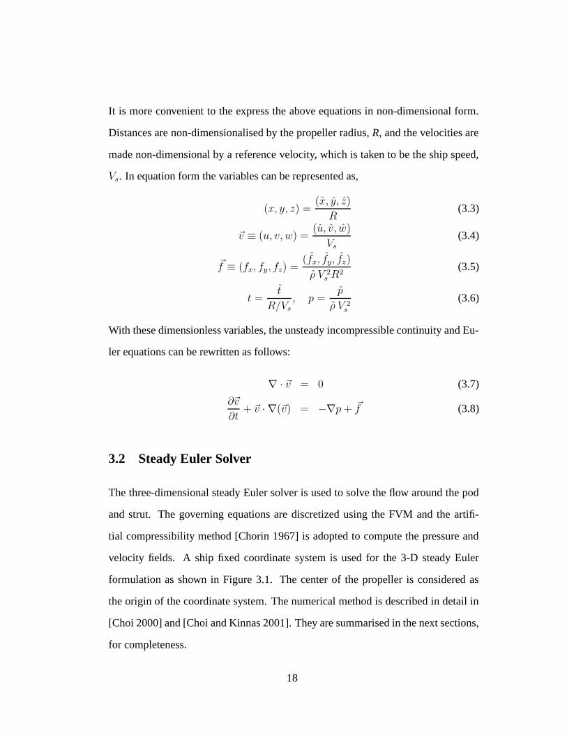
It is more convenient to the express the above equations in non-dimensional form.
Distances are non-dimensionalised by the propeller radius, R, and the velocities are
made non-dimensional by a reference velocity, which is taken to be the ship speed,
Vs. In equation form the variables can be represented as,
(x, y, z) =(x, y, z)
R(3.3)
~v ≡ (u, v, w) =(u, v, w)
Vs
(3.4)
~f ≡ (fx, fy, fz) =(fx, fy, fz)
ρ V 2s R
2(3.5)
t =t
R/Vs, p =
p
ρ V 2s
(3.6)
With these dimensionless variables, the unsteady incompressible continuity and Eu-
ler equations can be rewritten as follows:
∇ · ~v = 0 (3.7)
∂~v
∂t+ ~v · ∇(~v) = −∇p+ ~f (3.8)
3.2 Steady Euler Solver
The three-dimensional steady Euler solver is used to solve the flow around the pod
and strut. The governing equations are discretized using the FVM and the artifi-
tial compressibility method [Chorin 1967] is adopted to compute the pressure and
velocity fields. A ship fixed coordinate system is used for the 3-D steady Euler
formulation as shown in Figure 3.1. The center of the propeller is considered as
the origin of the coordinate system. The numerical method is described in detail in
[Choi 2000] and [Choi and Kinnas 2001]. They are summarised in the next sections,
for completeness.
18

����������������������������������������������������������������������
����������������������������������������������������������������������θ
Ship
propeller plane
y
x
z
Figure 3.1: Ship-fixed Cartesian coordinate system (taken from [Choi 2000])
A cartesian coordinate system is used for the 3-D formulation, while a cylindrical
coordinate system is used for the axisymmetric formulation.
3.2.1 Axisymmetric Steady Euler Solver
The axisymmetric Euler solver is used to solve the flow around axisymmetric bodies
like the pod without the strut. The artificial compressibility method [Chorin 1967] is
used to solve the Euler equations. In this method the incompressible flow equations
are given a hyperbolic character (changed from their mixed parabolic-elliptic char-
acter) by adding a pseudo time derivative of the pressure. At convergence, the time
derivative is zero and the solution satisfies the incompressible flow equations. The
addition of pseudo unsteady terms to the Euler equations gives the following form
to the governing equation:
∂U
∂t∗+∂F
∂x+∂G
∂r= Q (3.9)
19

with
U =
rp
rux
rur
ruθ
, F =
rux/β
r(u2x + p)
ruxur
ruxuθ
, G =
rur/β
ruxur
r(u2r + p)
ruruθ
, (3.10)
Q =
0
rfx
u2θ + rfr
−uruθ + rfθ
The term β is the artificial compressibility parameter which has a constant value.
The smaller the β, the more “incompressible” the equations are. The value of β is
kept between 0.07 and 0.1 [Choi 2000].
3.2.2 Three-dimensional Steady Euler-Solver
The method of artificial compressibility [Chorin 1967] is applied again in the three-
dimensional steady Euler solver. The 3-dimensional governing equations are similar
to the axisymmetric equations except that there are three components now. The
form of the dimensionless governing equation, after the addition of the pseudo time
derivative is:
∂U
∂t∗+∂F
∂x+∂G
∂y+∂H
∂z= Q (3.11)
The terms U, F, G, H, and Q are defined as follows.
U =
p
u
v
w
, F =
u/β
u2 + p
uv
uw
, G =
v/β
uv
v2 + p
vw
, (3.12)
20

H =
w/β
uw
vw
w2 + p
, Q =
0
fx
fy
fz
The application of a finite volume scheme leads to the application of the divergence
theorem on the Euler equations. The integral form of the equations read as:
∂
∂t
∫∫∫
VUdV +
∫∫
S(Fnx + Gny + Hnz) dS =
∫∫∫
VQdV (3.13)
The fluid domain is discretized into hexahedral cells.The unit surface normal vector,
~n, with components (nx,ny,nz), points in the outward direction from the cell. The
discretisation in space is carried out by applying the equation over each cell. A
second order discretisation is used in space. Ni’s Lax-Wendroff method [Ni 1982]
is applied for the time discretisation. That is, the variable U at a particular node and
at the next time (pseudo-time) step n + 1, is approximated by the following second
order difference,
Un+1(i,j,k) ' Un
(i,j,k) +
(
∂U
∂t
)n
(i,j,k)
∆t +
(
∂2U
∂t2
)n
(i,j,k)
(∆t)2
2(3.14)
where, ∆t is the time step size, and the superscript n represents the value at the
current time step. Since this is a second order scheme in space, artificial dissipation
is added to the solution to stabilise it. A second and fourth order dissipation, µ2 and
µ4, are scaled by time and added to the discretised formula:
Un+1(i,j,k) ' Un
(i,j,k) +∑
cells
δUn(i,j,k) + ∆t(µ2 − µ4) (3.15)
The solution around the pod and strut is solved using 3-D Euler solver called
GBFLOW-3D, and its latest version can handle hull or tunnel boundaries, contra-
rotating propellers, stator-rotor combinations, ducted and podded propulsors [Gu
et al. 2003].
21

(u,v
)=(u
,v) gi
ven
∂(u,v,p)/∂n=0
∂(u,
v,p)
/∂n=
0
∂u/∂r=0∂p/∂r=0v=0
∂qt/∂n=0∂p/∂n=0
∂p/∂
n=0
Figure 3.2: 2-D grid showing the boundary conditions used for the axisymmetricEuler solver
3.2.3 Boundary Conditions
Axisymmetric solver
Figure 3.2 shows the boundary conditions used for the axisymmetric run. The
boundary conditions are as follows:
• Inflow or upstream boundary
The velocities are set to a given value, and the first derivative of the pressure with
respect to the axial direction is taken equal to zero.
(u, v) = (u, v)given
∂p
∂n=∂p
∂x= 0 (3.16)
where, (u, v)given are the components of the inflow far upstream of the podded
propulsor.
22

• Outflow or downstream boundary:
The derivatives of all the velocity components and the pressure with respect to the
axial direction are taken equal to zero.
∂(u, v, p)
∂n=∂(u, v, p)
∂x= 0 (3.17)
• Axis of Rotation/Bottom boundary
For the axisymmetric solver, the first derivative of the axial velocity and the pressure
along the radial direction are taken equal to zero. The radial velocity is taken equal
to zero.
∂u
∂r= 0
∂p
∂r= 0
v = 0 (3.18)
• Top/Far-stream boundary
The derivatives of the velocity components and the pressure along the normal direc-
tion at the boundary are taken equal to zero.
∂(u, v, p)
∂n= 0 (3.19)
• Hull (or pod) boundary
A free-slip boundary condition is imposed on the pod. The derivatives of the tangen-
tial velocity and the pressure along the normal direction at the boundary are taken
23

equal to zero.∂qt∂n
= 0 ,∂p
∂n= 0 (3.20)
The tangential velocity derivative actually should include the effect of curvature
which are ignored here but can be found in [Kinnas, Lee, Gu, Yu, Sun, Vinayan,
Kacham, Mishra and Deng 2004].
3D-solver
Figure 3.3 shows the boundaries in the three-dimensional Euler solver. Boundary
conditions need to be applied on seven boundaries as stated below
• The upstream boundary where the flow enters the domain (Inflow)
• The downstream boundary where the flow leaves the domain (Outflow)
• The hull boundary at the top
• The outer boundary, or the far field (under the pod)
• The centerline boundary (this is the boundary along the axis of the pod, before
the pod leading edge and after the pod trailing edge)
• The pod and strut boundary
• The periodic boundary which connects the beginning and the end of the in-
dices along the circumferential direction (this occurs before the strut leading
edge and after the strut trailing edge, as shown in Figure 3.5).
The applied boundary conditions are shown in Figure 3.3. The top boundary is
treated as a hull, while the side and bottom boundaries are treated as far-stream
24

Far stream B.C. ∂(u,v,w,p)--------------=0
∂n
Out
flow
B.C
.
X
Y
Z
Strut
Pod
Hull B.C
∂(p)q.n=0, ----- = 0
∂(n)
Center line bndry (j=1)
i-index
j=1 j=1
Inflo
wU
x
Figure 3.3: Boundary conditions for the Euler solver which evaluates the flowaround the pod and strut in the presence of the propeller, (taken from [Gupta 2004]).
boundaries (they should be located sufficiently far from the propeller and pod plane
as shown in Figure 3.4).
The boundary conditions applied in the present method are summarized next
• Upstream boundary
Each velocity component is set to a given value, and the first derivative of the pres-
sure with respect to the axial direction is taken equal to zero.
(u, v, w) = (u, v, w)given (3.21)
∂p
∂n=∂p
∂x= 0 (3.22)
where, (u, v, w)given are the components of the inflow far upstream. A first order
differencing scheme is used, i.e. the pressure value at the second i index (i.e. i = 2)
25

X
Y
Z
Hull B.C∂(p)
(q.n=0), ------- =0∂n
FA
RS
TR
EA
M
FA
RS
TR
EA
M
n
n
K-in
dex
J-index
Strut
Far stream B.C. ∂(u,v,w,p)--------------=0
∂n
Figure 3.4: Boundary conditions on the domain at an axial location showing podand strut (no repeat boundary), (taken from [Gupta 2004])
is taken equal to that at the first index (i.e. i = 1).
• Downstream boundary:
The derivatives of all the velocity components and the pressure with respect to the
axial direction are taken equal to zero.
∂(u, v, w, p)
∂n=∂(u, v, w, p)
∂x= 0 (3.23)
Similar to the case of the upstream boundary, the derivatives are evaluated using a
first order differencing scheme.
• Center line boundary (j=1 line in the grid):
26

Far stream B.C. ∂(u,v,w,p)--------------=0
∂n
X
Y
Z
Hull B.C∂(p)
(q.n=0), ------- =0∂n
FA
RS
TR
EA
M
FA
RS
TR
EA
M
n
n
K-in
dex
J-index
K=1,nkRepeat Bndry
Figure 3.5: Boundary conditions on the domain at an axial location showing therepeat boundary (k = 1, Nk), (taken from [Gupta 2004])
In the case of the axisymmetric solver, the first derivatives of the axial velocity and
pressure along the radial direction as well as the tangential and radial velocities are
taken equal to zero. In the case of the three-dimensional solver, the values of the
velocities and pressure at the center boundary (j = 1) are taken equal to the average
of the values at (j = 2), over all (k = 1 to Nk), as shown next.
(u, v, w, p)(i,1,k) =1
Nk
∑
k=1,Nk
(u, v, w, p)(i,2,k) (3.24)
where, Nk is the number of nodes in the circumferential direction.
• Far-stream boundary :
27
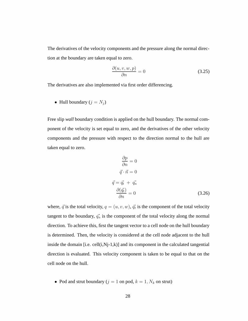
The derivatives of the velocity components and the pressure along the normal direc-
tion at the boundary are taken equal to zero.
∂(u, v, w, p)
∂n= 0 (3.25)
The derivatives are also implemented via first order differencing.
• Hull boundary (j = Nj)
Free slip wall boundary condition is applied on the hull boundary. The normal com-
ponent of the velocity is set equal to zero, and the derivatives of the other velocity
components and the pressure with respect to the direction normal to the hull are
taken equal to zero.
∂p
∂n= 0
~q · ~n = 0
~q = ~qt + ~qn
∂(~qt)
∂n= 0 (3.26)
where, ~q is the total velocity, q = (u, v, w), ~qt is the component of the total velocity
tangent to the boundary, ~qn is the component of the total velocity along the normal
direction. To achieve this, first the tangent vector to a cell node on the hull boundary
is determined. Then, the velocity is considered at the cell node adjacent to the hull
inside the domain [i.e. cell(i,Nj-1,k)] and its component in the calculated tangential
direction is evaluated. This velocity component is taken to be equal to that on the
cell node on the hull.
• Pod and strut boundary (j = 1 on pod, k = 1, Nk on strut)
28

The boundary condition on the pod and strut boundaries shown in Figure 3.4 is
similar to the hull boundary condition. The pod and strut is considered as a wall,
and the flow should not penetrate the wall. To achieve this, the normal component of
the velocity is set equal to zero, and the derivatives of the other velocity components
and the pressure with normal direction to the boundary are put as zero. The equation
used is the same as equation 3.26.
• Periodic or Repeat boundary as shown in Figure 3.5 (three-dimensional prob-
lem only):
(u, v, w, p)k=1 = (u, v, w, p)k=Nk(3.27)
where k is the index along the circumferential direction.
3.3 Vortex Lattice Method
This section presents an overview of the vortex lattice method based potential flow
solver which is used for the analysis of the cavitating propeller flow. The complete
formulation of the potential flow solver and the vortex lattice method may be found
in chapter 6 by Kinnas in the book of [Ohkusu 1996].
The vortex lattice method which solves for the unsteady potential flow field around a
cavitating propeller has been used successfully since the method was first developed
in [Kerwin and Lee 1978], [Lee 1979] and [Breslin et al. 1982].
In the vortex lattice method, a special arrangement of line vortex and source lattice
is placed on the blade mean camber surface and its trailing wake surface. There are
three types of singularities:
29

(a) the vortex lattice on the blade mean camber surface and the trailing wake surface
which represents the blade loading and the trailing vorticity in the wake,
(b) the source lattice on the blade mean camber surface which represents the blade
thickness, and
(c) the source lattice throughout the predicted sheet cavity domain which represents
the cavity thickness.
This method is classified as a lifting surface method because the singularities (vor-
tices and sources) are distributed on the blade mean camber surface, as opposed to
the other class of method, the surface panel method, in which the singularities are
distributed on the actual blade surface.
The unknown strengths of the singularities are determined so that the kinematic and
the dynamic boundary conditions are satisfied at the control points on the blade mean
camber surface.
The Kinematic Boundary Condition requires that the flow velocity be tangent to the
mean camber surface, and is applied at all control points.
The Dynamic Boundary Condition requires that the pressure on the cavitating part
of the blade mean camber surface be equal to the vapor pressure, and is applied only
at the control points that are in the cavitating region.
3.4 Boundary Element Method
The numerical formulation for the Boundary Element Method (BEM) used to solve
for the flow around the pod and strut, in the absence of the propeller, subject to inflow
30

at zero yaw angle was presented in [Gupta 2004]. The method has been summarized
in this section for completeness.
3.4.1 Formulation of Potential Flow around a Pod and Strut
The fluid flow field around an axisymmetric pod and a 3-D pod and strut unit without
the presence of a propeller, with uniform inflow, can be solved using the BEM.
The flow around the pod and strut is assumed to be incompressible, inviscid and
irrotational. Then, the fluid domain can be represented by using the perturbation
potential φ(x, y, z), defined as follows:
~q(x, y, z) = ~Uin(x, y, z) + ∇φ(x, y, z) (3.28)
where ~q is the total velocity and ~Uin is the inflow velocity to the pod and strut
The perturbation potential has to satisfy Laplace’s equation inside the fluid domain,
as follows,
∇2φ = 0 (3.29)
The effect of wake of the strut is not considered since the inflow is along the pod
axis.
The potential on the pod and strut satisfies the equation 3.30, which is obtained from
Green’s third identity.
2πφp =∫
SB
[
φq∂G(p; q)
∂n− G(p; q)
∂φq
∂n
]
dS (3.30)
where points p and q correspond to the field and variable points respectively on the
integration. G(p;q) = 1/R is the Green’s function, R(p;q) is the distance between the
31

points p and q, and ~n is the normal vector to the surface of the body SB pointing into
the field domain.
The above integral equation is discretized using quadrilateral panels with constant
strength dipole and source distributions over each panel on the pod and strut sur-
faces.
3.4.2 Kinematic Boundary Condition on the Body
The kinematic boundary condition requires that the flow is tangent to the body and
there are no normal velocity components to the wall. Hence,
∂φ
∂n= −~Uin · ~n (3.31)
where ~n is the normal vector on the body surface pointing into the fluid.
3.4.3 Kutta Condition
The Kutta condition requires that the velocity at the trailing edge (T.E.) of the rudder
to be finite.
∇φ is finite at T.E. (3.32)
The Kutta condition could be enforced numerically by applying the Morino condi-
tion [Morino and Kuo 1974], which requires the difference of the potentials at the
two sides of the trailing edge to be equal to the potential jump in the wake. However,
for the case with zero degree angle of attack, ∇φ does not exist at the trailing edge
and hence equation 3.32 is not required due to symmetry.
32

3.4.4 Hull Effects
The strut of the pod in 3-D is assumed to be attached to a flat hull on the top. Hence,
to include the hull effects the image of the pod with respect to the hull must be
considered. The advantage of this approach is that the hull does not need to be
modeled directly, but only the influence coefficients for each source and dipole panel
need to be changed to include those of their images.
3.5 FLUENT
FLUENT is a commercial CFD package that is used for various CFD applications
and problems. In this section the numerical schemes applied to solve the flow field
with the propeller included via body forces are discussed. FLUENT is used both
as an inviscid and a viscous flow solver in this case. FLUENT solves the RANS
equations. The Navier-Stokes (N-S) equation are transformed so that the small scale
turbulent fluctuations are not directly simulated, but Reynolds Averaging is carried
out. The Reynolds Averaged Navier-Stokes (RANS) equations represent transport
equations for the mean flow quantities only, with all the scales of the turbulence
modeled. In Reynolds averaging, the solution variables in the exact N-S equations
are decomposed into the mean, ui and fluctuating components ui. Hence the param-
eters can be written as,
ui = ui + u′i (3.33)
Substituting expressions of this form for the flow variables into the instantaneous
continuity and momentum equations and taking a time average yields the RANS
33

equations which are shown below,
∂ρ
∂t+∂ρui
∂xi
= 0 (3.34)
∂ρui
∂t+∂ρuiuj
∂xj
=
−∂p
∂xi
+∂
∂xj
[µ(∂ui
∂xj
+∂uj
∂xi
−2
3δij∂ul
∂xl
)] +∂
∂xj
(−ρui′uj
′) (3.35)
In FLUENT various solver options are available. The details of those can be found
in [FLUENT 2003] solver options used are,
• Segregated solver: The governing equations are solved in a sequence i.e. sep-
arately from each other using a finite volume method.
• Pressure Equation: The SIMPLE algorithm is used, which uses a relationship
between the velocity and pressure corrections to enforce mass conservation
and obtain the pressure field.
• Spatial Discretisation: A Second-Order Upwind scheme is used in FLUENT
for spatial discretisation. In FLUENT this is achieved at cell faces through a
Taylor series expansion of the cell centered solution about the cell centroid.
Hence the face value uf is computed as,
uf = u+ ∇u · ∆~s (3.36)
where u and ∇u are the value at the cell center and its gradient at the upstream
cell, and ∆~s is the displacement vector from the upstream cell centroid to the
face centroid.
• Turbulence Model: The k− ε and ReynoldsStressModel(RSM) turbulence
models are used for viscous cases in our problem. The k − ε model is a two
34

equation model in which the solution of two separate transport equations al-
lows the turbulent velocity and length scales to be independently determined.
It is a semi-empirical model. Details of the calculation of parameters for this
model are provided in Section 4.2.3. The RSM model closes the RANS equa-
tions by solving the transport equations for the Reynolds stresses, together
with an equation for the dissipation rate. This results in five additional equa-
tions in 2D flows.
3.6 Coupling to determine pod and propeller interaction
In the present methods, the effective inflow is used as the propeller inflow. To
achieve this, first the induced velocities, due to the propeller sources and dipoles,
are calculated at the effective wake location. The solution from the Euler or RANS
solver gives the total velocity at that location. Subtracting the propeller induced
from the total velocities, the effective velocity is obtained. In this coupled Euler or
RANS/potential flow calculation, the propeller is solved by using the VLM based
potential solver MPUF-3A. The inviscid flow field around the propeller and pod
unit is solved using the Euler solver GBFLOW-3X or 3D or inviscid FLUENT. The
viscous flow field around the podded unit is calculated using viscous FLUENT.
3.6.1 GBFLOW or FLUENT/MPUF-3A coupling
The coupling of GBFLOW or FLUENT with MPUF3A provides a way of analyzing
the interactions among propeller, pod and strut. In the coupling MPUF3A is first
solved for the potential flow distribution around the propeller and the pressure dis-
tributions on the blade are evaluated. The pressure distributions are then converted
35

Potential SolverPotential Solver
X
Y
Z
Strut
Pod
Xeff
Xeff
3-D Euler Solver
Figure 3.6: Pictorial representation of the coupling of the Finite Volume Method andthe Vortex Lattice Method (from [Kinnas, Gu, Gupta and Lee 2004]).
into body force terms which represent the propeller in GBFLOW or in FLUENT. In
FLUENT this is done by defining a User-Defined Function which incorporates the
source terms in the Euler/RANS equations. GBFLOW or FLUENT is then solved,
with the body force terms and appropriate boundary conditions, in the whole fluid
domain which includes the pod and strut. From the solution, the total velocity at
the effective wake location for each propeller is obtained. The propeller induced
velocities are calculated via MPUF-3A, by summing the effects of all singularities
representing the blade and its wake. The effective velocity is then calculated as the
difference of the total from the propeller induced velocity. This is now used as the
new inflow velocity to each propeller. Iterations are carried out between the meth-
ods till convergence is achieved. A pictorial representation of the iterative process is
shown in Figure 3.6 [Kinnas, Gu, Gupta and Lee 2004].
36

Interpolation of body forces in FLUENT
As mentioned earlier, the pressure distribution obtained from MPUF3A is converted
into body forces which are then incorporated into GBFLOW/FLUENT. This incor-
poration in FLUENT is done via GBFLOW. Once the body forces are calculated by
GBFLOW, and as the grids of GBFLOW and FLUENT are not the same, interpo-
lation is carried out to assign body forces to cells in FLUENT. In GBFLOW, the
body forces are known at the nodes of the GBFLOW grid. However, FLUENT is
a cell centered scheme. The location of the cell centroids in the FLUENT grid is
first determined. Then linear interpolation in both directions, x and r is carried out
between the data available from GBFLOW and the interpolated body forces are as-
signed to the cell centroids in the FLUENT grid. This coupling with FLUENT has
been carried out only for the case of axisymmetric flow.
3.6.2 Coupling of Non-dimensional Forces from FVM and VLM
The propeller force given by MPUF-3A is in the form of KT and KQ values, where
KT is the thrust coefficient and KQ is the torque coefficient. KT is defined as
KT =F
ρn2D4(3.37)
where D is the diameter of the propeller and n is the number of revolutions per
second of the propeller. The advance ratio Js is defined as
Js =Vs
nD(3.38)
To couple the forces obtained from GBFLOW-3D and MPUF-3A, both should be
non-dimensionalized in a similar manner. Non dimensional force in GBFLOW is
37

given by equation 3.5
FGB ≡ (fx, fy, fz) =(fx, fy, fz)
ρ V 2s R
2
using equation 3.37 and equation 3.38,we get
KT =F
ρn2D2D2=
F
4ρV 2s
J2s
R2=
F
ρV 2s R
2×J2
s
4= FGB ×
J2s
4(3.39)
In GBFLOW the frictional force on the surface of the pod and strut is evaluated by
using the formula:
FFR = CfρV2s S (3.40)
where, S is the surface area of the pod and strut, and Cf is a uniformly applied
frictional coefficient, provided by the ITTC formula (equation 4.7). Making the
equation 3.40 non-dimensional, we get
FFRND =CfρV
2s S
ρV 2s R
2(3.41)
FFRND =CfS
R2(3.42)
On the other hand, FLUENT is a dimensional code and all input and output obtained
from FLUENT are in dimensional form. Hence they need to be handled appropri-
ately. The first step is to dimensionalise the pressure forces obtained from the VLM
and convert them to dimensional body forces. This is carried out in two steps. First,
the forces from VLM are converted to body forces in a similar manner as done for
GBFLOW and the non-dimensionalising is as shown in equation 3.5. Next the body
forces are converted to dimensional form in the User Defined Function as,
FFL = FGB × ρ V 2s R
2≡ (fx, fy, fz) × ρ V 2
s R2 (3.43)
38

Once the solution is obtained from FLUENT and the total flow field is known, the
velocities are to be used to calculate the effective wake. Accordingly, the velocities,
~VFL, resulting from FLUENT are non-dimensionalised as,
U = VFL/Vs (3.44)
3.6.3 BEM/MPUF3A coupling
The coupling between BEM (applied on the pod) and MPUF-3A (applied on the pro-
peller) is carried out via induced potentials and induced velocities. More specifically
the pod affects the propeller via induced velocities and the propeller affects the pod
via induced potentials. This problem is also solved iteratively. This approach should
help estimate the accuracy of the currently implemented image model in MPUF-3A.
In the iterative procedure, first, MPUF-3A is solved to obtain the potential flow dis-
tribution around the propeller. The singularities associated with the blade and wake
are known at this point. Next, the potentials induced by these singularities at the
pod control points are calculated. After this has been done the pod problem can be
solved as detailed in Section 3.4. The pod problem is now solved in a system with
respect to the propeller. In addition the flow is also treated as non-axisymmetric.
The governing equation 3.30 is now modified to account for the propeller effect via
induced potentials. Accordingly the new equation is,
2πφp =∫
SB
[
φq∂G(p; q)
∂n− G(p; q)
∂φq
∂n
]
dS + 4πφpr (3.45)
where φpr is the propeller induced potential at control point P .
The next step involves calculating the induced velocities at the blade control points
due to the source and dipole distribution on the pod panels. MPUF-3A should then
39
be solved next, after accounting for the pod effect. This is done by modifying the
kinematic boundary condition for the VLM. The new equation now is,
∑
Γ
Γ~v · ~n = −~qt · ~n (3.46)
where ~qt is the inflow velocity plus the pod induced velocity which has been modi-
fied to include the velocities induced by the pod, ~n is the unit normal vector and Γ is
the constant strength of each bound vortex. Iterations are carried out till a converged
solution is obtained. The iterative procedure is shown in Figure 3.7. This procedure
has been successfully implemented in the past by [Kerwin et al. 1987]. However the
implementation has been unsuccessful in this case.
40

BEMMPUF3A
1a. Solve BEM. Find potentials on pod.Find pod panel CP’s
1b. Solve MPUF3A. Find blade geometrydata. Output KBC CP’s.
2. Calculate Induced velocities on blade CP’s3.Solve MPUF3A with inducedvelocities added to RHS matrix
4. Calculate induced potentialby blade on pod CP’s5. Update RHS matrix of BEM and solve
STOPconverged not converged
Figure 3.7: Pictorial representation of the coupling of the Boundary Element Methodand the Vortex Lattice Method.
41

Chapter 4
Validation and Comparisons with Other Methods -Axisymmetric Pod
In this chapter comparisons are carried out among different axisymmetric codes,
GBFLOW-3X, FLUENT and BEM. Validation of results from GBFLOW-3X is car-
ried out by comparing on-pod and off-pod velocities and pressures with those ob-
tained from FLUENT and BEM. Convergence studies are also carried out for all the
methods. Viscous FLUENT is used to estimate the effects of viscosity. The changes
in the flow field are observed but more importantly the pressures and shear stress
distributions along the pod are studied. This is so because the frictional force on the
pod is calculated in GBFLOW-3X using the ITTC friction formula and the accuracy
of this simplification has to be assessed.
4.1 Axisymmetric Euler Solver
In the axisymmetric Euler solver, it is assumed that the pod is an axisymmetric body
and the presence of the strut is ignored. The axisymmetric Euler Solver, called
GBFLOW-3X, uses similar equations as the fully 3-D equations. Therefore, for the
fully 3-D Euler solver to be correct, it is pertinent that the axisymmetric Euler solver
42

provide accurate results. The main benefit of using GBFLOW-3X is the smaller
computing times than those associated with GBFLOW-3D.
The pod is assumed to be at the center of the domain. A wall (or a hull) condition
which is a free slip condition given by equation 3.26 is applied on the pod, and far
field conditions given by equation 3.25 are applied at those boundaries.
4.1.1 Grid and Boundary Conditions
Grid Generation
Figure 4.1 shows the grid for the axisymmetric Euler solver, which is symmetric
about the axis of the pod. More cells have to be concentrated near the leading edge
and trailing edge of the pod to capture the expected stagnation points. Since the fine
resolution of grid points is not required near the inflow and outflow boundaries, an
expansion ratio is used from the leading edge of the pod to the inflow boundary, and
from the trailing edge to the outflow boundary, as shown in Figure 4.2. Along the
j direction, denser grid is required close to the pod, than at the far field. Therefore
the grid, as shown in Figure 4.1, is made uniform up to y=1.0 (the propeller radius),
and an expansion ratio is used thereafter. The geometry of the pod used for the
axisymmetric runs is given in Appendix A and is the one used by Szantyr [Szantyr
2001b] for the experiments carried out at the Technical University of Gdansk.
The offsets of the pod (radius versus axial locations) are passed to the grid gener-
ation code. The grid points on the pod are then interpolated using a spline scheme
developed by Lee, H. S. and Natarajan, S. (personal communication).
43

Inflo
w(u
)
Top Boundary (far field)
Out
flow
Pod
jin
crea
sing
i increasing
Figure 4.1: 2-D grid showing the boundaries for the axisymmetric Euler solver
AXIS
Leading Edge
POD
Leading Edge
Expansion Ratio Cosine SpacingAXIS
Trailing Edge
POD
Trailing Edge
Expansion Ratio Cosine Spacing
Figure 4.2: Closeup of the leading and trailing edge showing the uniform expansionratio.
44

Boundary Conditions
The top boundary is treated as far stream boundary. The left side boundary is the
inflow, while the right boundary is the outflow. The bottom is considered as an
axis of rotation. The only components of velocity required in the axisymmetric
case are the axial and the radial components. Since this is axisymmetric flow the
circumferential component is equal to zero (in the absence of a propeller). The
details of the boundary conditions were presented in Section 3.2.3.
4.1.2 Results
GBFLOW-3X is run with different grids to obtain the flow field around the pod and
the pressure force on it. As this is an inviscid solver, ideally the pressure force should
be zero. However, due to discretisation errors this is not the case.
Figures 4.4 and 4.5 show the convergence of axial velocities and pressures on the
body respectively, with different grids (with the number of axial nodes varied).
Close-up of the different grids over the body and near the leading edge is shown
in Figure 4.3.
The axial velocity and pressure contours are shown in Figures 4.6 and 4.7, respec-
tively for the grid with 140 × 81 nodes.
The total pressure force on the axisymmetric body is calculated by integrating the
pressure force over the pod. Table 4.1 shows the pressure forces obtained for differ-
ent grids. Effectively these values are the discretisation errors (as the force ideally
should be zero) and hence can be viewed as a convergence criteria for the grids. It
is seen that with increasing resolution the calculated force decreases.
45

x
y
-1 0 1
-0.5
0
0.5
1
140 x 81
x
y
-1 0
-0.5
0
0.5
1
150 x 81
x
y
-1 0 1
-0.5
0
0.5
1
180 x 81
x
y
-1 0
-0.5
0
0.5
1
100 x 81
Figure 4.3: Close-up of different grids (near the leading edge) used for convergencestudies in GBFLOW-3X without propeller
Grid Size Pressure Force
I × J
100x81 2.88 × 10⁻⁴
140x81 1.5909 × 10⁻⁴
150x81 1.2396 × 10⁻⁴
180x81 1.2565 × 10⁻⁴
Table 4.1: Total force on the pod from Euler solver for axisymmetric runs for differ-ent grid densities. Forces made non-dimensional as given by equation 3.5
46

X
U
-1 0 1 2 3
0.6
0.65
0.7
0.75
0.8
0.85
0.9
0.95
1
100 x 81140 x 81150 x 81180 x 81
Figure 4.4: Convergence of axial velocities on body with different grids inGBFLOW-3X (number of nodes in axial direction is varied)
4.2 FLUENT
To validate the results of GBFLOW-3X it is essential to carry out comparisons with
other methods. Inviscid axisymmetric version of FLUENT is used towards this pur-
pose while viscous version of FLUENT is used to study the effects of viscosity on
the flow field and the pressures and forces on the pod.
47

X
Cp/2
-4 -3 -2 -1 0 1 2 3 4 5 6 7-0.05
0
0.05
0.1
0.15
0.2
0.25
0.3
0.35
0.4 100 x 81140 x 81150 x 81180 x 81
Figure 4.5: Convergence of pressure on body with different grids in GBFLOW-3X(number of nodes in axial direction is varied)
4.2.1 Grid and Boundary Conditions
When inviscid runs are carried out with FLUENT, an unstructured grid is used. The
main advantage of using an unstructured grid over structured grids is that it gives
smoother discretisation near the leading and trailing edges and hence more cells can
be concentrated near these regions. However, when inviscid runs are carried out with
body forces (representing a propeller), a structured and finer grid is needed to obtain
good results as shown in Chapter 5. Also it was desirable to compare the results
from GBFLOW-3X and FLUENT using the same grid. Hence, the grid generated
48

x
y
-2 -1 0 1 2 3 4-1
0
1
2
3
4
u10.950.90.850.80.750.70.650.60.550.50.450.40.350.30.250.2
Figure 4.6: Axial velocity contour around the body from GBFLOW-3X
by GBFLOW-3X was exported to GAMBIT (grid generation code for FLUENT).
So a structured grid was also used and results were compared with the unstructured
one. In case of a viscous run, the unstructured grid has a boundary layer attached to
the pod to capture the viscous effects as shown in Figure 4.9.
Table 4.2 gives the parameters used in FLUENT for the inviscid case. Figures 4.84.9
and 4.10 show the unstructured grid used in FLUENT and a blow up near the leading
edge to show the boundary layer and concentration of cells. The structured grid is
shown in Figure 4.11. An expansion ratio is used on either side of the body. On the
pod, a double sided expansion is used so as to concentrate more cells near the leading
and trailing edges. In the y-direction, constant spacing is used till the propeller radius
and then an expansion ratio is employed.
The boundary conditions are also given in Table 4.2. The left boundary in assumed
49

x
y
-3 -2 -1 0 1 2 3 4 5-1
0
1
2
3
4
5p
0.360.320.280.240.20.160.120.080.040
Figure 4.7: Pressure contour around the body from GBFLOW-3X
to be the inflow to the domain, and is set to
u = 1.0; v = 0.0 (4.1)
The top boundary is treated as a free stream boundary and assuming that there is no
effect of the pod at that location, and hence, the boundary conditions are the same
as given by equation 4.1. The outflow boundary on the right side of the domain is
given as a pressure outlet condition:
∂p
∂x= 0 (4.2)
For the pod, a wall boundary condition is given. This is a slip condition for the
inviscid case, and a no-slip condition for the viscous case.
50
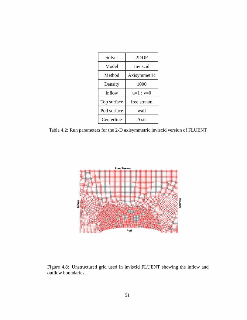
Solver 2DDP
Model Inviscid
Method Axisymmetric
Density 1000
Inflow u=1 ; v=0
Top surface free stream
Pod surface wall
Centerline Axis
Table 4.2: Run parameters for the 2-D axisymmetric inviscid version of FLUENT
Free Stream
Inflo
w
Ou
tflo
w
Pod
Figure 4.8: Unstructured grid used in inviscid FLUENT showing the inflow andoutflow boundaries.
51

Free Stream
Inflo
w
Ou
tflo
w
Pod
Figure 4.9: Unstructured grid used in viscous FLUENT showing the inflow andoutflow boundaries.
4.2.2 Results
Figures 4.12 and 4.13 show the convergence of the axial velocity and the pressure
with unstructured grids, respectively. The axial velocity and pressure contours are
shown in Figures 4.14 and 4.15 respectively.
Comparisons are carried out between the unstructured and structured grids to see
if there are any differences in the solution. Figures 4.16 and 4.17 show the axial
velocity and the pressure on the body obtained from both the grids. As can be seen
they are almost the same. Figure 4.18 shows the comparison of the axial velocity at
a y-plane location near the leading edge. They are almost the same, except near the
body but even there they show the same tendency.
The pressure forces obtained from inviscid runs are shown in Table 4.3 The veloc-
52

Pod
Figure 4.10: A closeup view of the grid near the pod, showing the boundary layerused and the triangular grid at the leading edge of the pod.
Figure 4.11: Structured grid used in FLUENT and exported from GBFLOW-3X
53
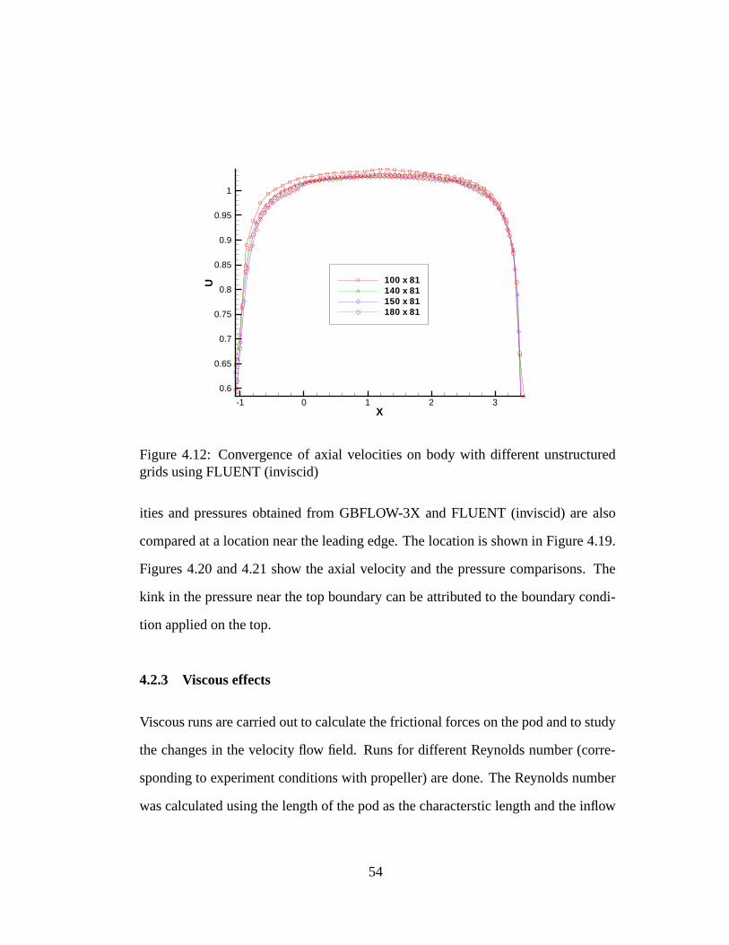
X
U
-1 0 1 2 3
0.6
0.65
0.7
0.75
0.8
0.85
0.9
0.95
1
100 x 81140 x 81150 x 81180 x 81
Figure 4.12: Convergence of axial velocities on body with different unstructuredgrids using FLUENT (inviscid)
ities and pressures obtained from GBFLOW-3X and FLUENT (inviscid) are also
compared at a location near the leading edge. The location is shown in Figure 4.19.
Figures 4.20 and 4.21 show the axial velocity and the pressure comparisons. The
kink in the pressure near the top boundary can be attributed to the boundary condi-
tion applied on the top.
4.2.3 Viscous effects
Viscous runs are carried out to calculate the frictional forces on the pod and to study
the changes in the velocity flow field. Runs for different Reynolds number (corre-
sponding to experiment conditions with propeller) are done. The Reynolds number
was calculated using the length of the pod as the characterstic length and the inflow
54

X
CP/2
-1 0 1 2 3-0.1
0
0.1
0.2
0.3
0.4
0.5
0.6
100 x 81140 x 81150 x 81180 x 81
Figure 4.13: Convergence of pressure on body with different unstructured grids us-ing FLUENT (inviscid)
velocity as the characteristic velocity. The viscous runs are done using the k − ε
model. The run parameters for viscous FLUENT are given in Table 4.4. The val-
ues of turbulence kinetic energy and turbulence dissipation rate are calculated from
equations 4.5 and 4.6. It is important that the Y + on the pod does not increase be-
yond the range where the wall functions in the boundary layer apply. Figure 4.22
shows the Y + on the body of the pod. The maximum value of Y + obtained by using
the k − ε method is 39, which is acceptable.
The dissipation constants are evaluated using the following equations.
Re =ρUT
µ(4.3)
where, T is the maximum length of the pod, and U is the velocity of the flow.
55

Grid Size Pressure Force
I × J
100x81 3.81 × 10⁻⁴
140x81 1.94 × 10⁻⁴
150x81 1.70 × 10⁻⁴
180x81 1.41 × 10⁻⁴
Table 4.3: Total force on the pod and the computed surface area from FLUENT foraxisymmetric runs for different grid densities.
Solver 2DDP
Model k − ε
Density 998.2
Viscosity 1 × 10⁻³
Cµ 0.09
Top surface free stream
Pod surface wall
centerline axis
Grid type mapped
Table 4.4: Run parameters for 2-D axisymmetric viscous FLUENT
56

X
Y
-2 -1 0 1 2 3 4
-1
0
1
2
3
4
1.000.940.890.830.770.710.660.600.540.490.430.370.310.260.20
Figure 4.14: Axial velocity contour and streamlines from inviscid FLUENT
Turbulence intensity I can be written as
I = 0.16(Re)−1
8 (4.4)
Turbulence kinetic energy k can be written as
k =3
2(UI)2 (4.5)
Turbulence length scale can be written as l = 0.07T , and turbulence dissipation rate
ε as
ε = C3/4µ
k3/2
l(4.6)
where Cµ ≈ 0.09. The theoretical frictional coefficient can be calculated using the
empirical ITTC friction formula
Cf =0.075
(logRe− 2)2(4.7)
57

X
Y
-2 -1 0 1 2 3 4 5 6-1
0
1
2
3
4
5
6
0.360.330.310.280.260.230.210.180.150.130.100.080.050.030.00
Figure 4.15: Pressure contour from inviscid FLUENT
Runs were carried out for the Reynolds number given in Table 4.5 and the corre-
sponding k and ε values.
The frictional force for all Reynolds numbers and the empirical force (used in the
inviscid codes) calculated from Equation 4.7 is shown in Table 4.6. As is seen the
values are very close to each other and the ITTC formula may be used for inviscid
cases with reasonable accuracy.
To see what effect viscosity has on the velocities, the axial velocities for inviscid
and viscous runs are compared at locations which would later serve as the effective
wake locations for the fore and aft propellers. These locations are shown in Figure
4.23. The comparison between the velocities is shown in Figures 4.24 and 4.25. It
can be seen that there is a small difference between the inviscid and viscous cases
at the first location, but this difference increases as we move to the second location.
58
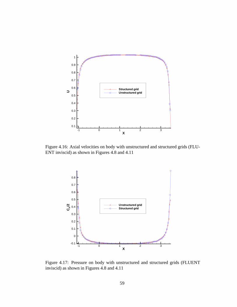
X
U
-1 0 1 2 30.1
0.2
0.3
0.4
0.5
0.6
0.7
0.8
0.9
1
Structured gridUnstructured grid
Figure 4.16: Axial velocities on body with unstructured and structured grids (FLU-ENT inviscid) as shown in Figures 4.8 and 4.11
X
CP/2
-1 0 1 2 3-0.1
0
0.1
0.2
0.3
0.4
0.5
0.6
0.7
0.8
Unstructured gridStructured grid
Figure 4.17: Pressure on body with unstructured and structured grids (FLUENTinviscid) as shown in Figures 4.8 and 4.11
59
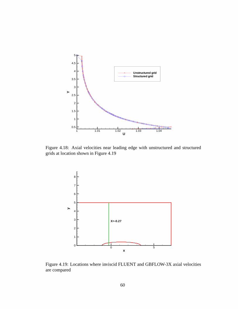
U
Y
1 1.01 1.02 1.03 1.040.5
1
1.5
2
2.5
3
3.5
4
4.5
5
Unstructured gridStructured grid
Figure 4.18: Axial velocities near leading edge with unstructured and structuredgrids at location shown in Figure 4.19
x
y
0 50
1
2
3
4
5
6
7
8
X=-0.27
Figure 4.19: Locations where inviscid FLUENT and GBFLOW-3X axial velocitiesare compared
60

Ux
Y
1 1.005 1.01 1.015 1.02 1.025 1.03 1.035 1.040.3
0.4
0.5
0.6
0.7
0.8
0.9
1
1.1
1.2
1.3
1.4
FLUENTGB
Figure 4.20: Comparison of axial velocities for inviscid FLUENT and GBFLOW-3Xat given location
Re k ε
6.26 × 10⁵ 0.0056 0.00021
8.24 × 10⁵ 0.009 0.00044
10.5 × 10⁵ 0.0138 0.00084
12.98 × 10⁵ 0.0200 0.00147
Table 4.5: Reynolds number, k and ε for which runs are carried out using viscousFLUENT
61

Cp/2
Y
-0.04 -0.03 -0.02 -0.01 0
0.5
1
1.5
2
2.5
3
3.5
4
4.5
5
FLUENTGBFLOW3X
Figure 4.21: Comparison of pressure for inviscid FLUENT and GBFLOW-3X atgiven location
X
Y+
-1 0 1 2 3
5
10
15
20
25
30
35
Figure 4.22: Y + on the pod for viscous FLUENT run, Re=4.5 × 10⁵
62

Re CfITTC k − ε
6.26 × 10⁵ 0.0096 0.0086
8.24 × 10⁵ 0.0088 0.0083
10.5 × 10⁵ 0.0082 0.0080
12.98 × 10⁵ 0.0077 0.0078
Table 4.6: Comparison of mean empirical frictional force coefficient Cf with thatfrom k − ε model
This will have a significant effect in the case when we have an aft propeller. The
discontinuity in the velocities predicted by the inviscid version of FLUENT near the
pod, as shown in Figure 4.24, could be due to the manner in which the slip boundary
condition is applied on the wall.
4.2.4 Study of different models
Figure 4.25 shows the difference between the axial velocity from the inviscid and
the viscous flow solver in the absence of the propeller. As can be seen the difference
is not as small as someone would expect. To study this, different turbulence models
in FLUENT were used. The RSM model and the k − ω were used which provided
results, much closer to the GBFLOW-3X result. This appears to be more accurate as
the changes between the inviscid and viscous solvers should be near the wall region.
The k − ε model was also run with a grid with a very low Y + = 6, but the solution
did not change much. The results are shown in Figure 4.25. So, a RSM model is
also used to solve the case of pod with propeller.
63

x
y
0 50
1
2
3
4
5
6
7
8
Xf=-0.415 Xa=1.93
Fore propeller Aft propeller
Figure 4.23: Locations for comparison of inviscid and viscous axial velocities
U
Y
0.8 0.85 0.9 0.95 10.3
0.4
0.5
0.6
0.7
0.8
0.9
1
1.1
1.2
FLUENT (κ−ε) Re=6.26x10⁵
FLUENT (κ−ε) Re=8.24x10⁵
FLUENT (κ−ε) Re=10.5x10⁵
FLUENT (κ−ε) Re=12.98x10⁵
FLUENT (Inviscid)FLUENT (RSM)GBFLOW-3X
Figure 4.24: Axial velocities for different Re at Xf=-0.415 location as shown inFigure 4.23.
64

U
Y
0.8 0.9 1 1.10.4
0.5
0.6
0.7
0.8
0.9
1
1.1
1.2
FLUENT (κ−ε)FLUENT (Inviscid)FLUENT (RSM)GBFLOW-3XFLUENT (κ−ω)
Figure 4.25: Axial velocities from different methods at Xa=1.93 location as shownin Figure 4.23, Re = 6.26 × 10⁵.
4.3 BEM
The computation using a Boundary Element Method (BEM) code is developed to
check the accuracy of the Euler solver. BEM, a potential solver, solves for the po-
tential on the body, which could be used to evaluate the velocities and pressures.
The main advantage of using BEM compared to the 3-D Euler solver is that the
CPU time can be remarkably reduced. The solver though essentially axisymmetric
carries out computations as a 3-D solver i.e. the influence coefficients are calculated
based on all the panel control points and the solution is carried out for the complete
matrix containing all the panel influence coefficients. Figure 4.26 shows the grid of
the pod for the BEM solver.
65

X Y
Z
Flow direction
Figure 4.26: Grid used for the axisymmetric BEM solver
4.3.1 Results
Convergence studies are performed to understand the behavior of the results and to
check their consistency. The dependence of axial velocity and pressures on the grid
discretization is shown in Figures 4.27 and 4.28 respectively. Table 4.7 gives the
total force from each grid obtained by integrating the non-dimensional pressures on
the surface of the body. The forces are made non-dimensional as FρU2S
, where S is
the surface area of the pod and U is the inflow velocity. It can be seen from the table
4.7 that with an increase of the grid panels on the pod, the pressure force reduces.
Ideally for an inviscid case, the pressure force on the pod should be zero.
Figure 4.29 shows the convergence of forces with grid size for all the different meth-
ods. All the methods seem to have approximately the same rate of convergence.
66

X
U
-2 -1 0 1 2
0.4
0.45
0.5
0.55
0.6
0.65
0.7
0.75
0.8
0.85
0.9
0.95
1
1.05
40 panels60 panels70 panels80 panels
Figure 4.27: Convergence of axial velocities with different grids using BEM
X
CP/2
-2 -1 0 1 2
-0.05
0
0.05
0.1
0.15
0.2
40 panels60 panels70 panels80 panels
Figure 4.28: Convergence of pressure with different grids using BEM
67

Grid Size Pressure Force
I × J
40x30 1.984 × 10⁻⁴
60x30 1.288 × 10⁻⁴
70x30 1.106 × 10⁻⁴
80x30 1.041 × 10⁻⁴
Table 4.7: Total force on the pod from BEM for axisymmetric runs for differentpaneling.
Number of cells/panels along pod
F/ρ
SV
2
40 50 60 70 800.0001
0.0002
0.0003
0.0004
BEMGBFLUENT
Figure 4.29: Convergence of forces with number of cells from all methods
68

4.4 Comparisons among different methods
The results from inviscid axisymmetric version of FLUENT are compared with the
results from GBFLOW-3X and from the BEM solver. An unstructured grid with
140 nodes on the pod was used for FLUENT, a grid with 140 × 81 nodes was used
for GBFLOW and a grid with 80 panels on the pod was used in the BEM. The
axial velocity and the pressures on the pod from FLUENT and the axisymmetric
BEM solver are compared with those from the axisymmetric Euler solver in Figures
4.30 and 4.31, respectively. The pressure obtained from FLUENT has to be non-
dimensionalized in a similar manner as done in GBFLOW as given by equation 3.6.
69
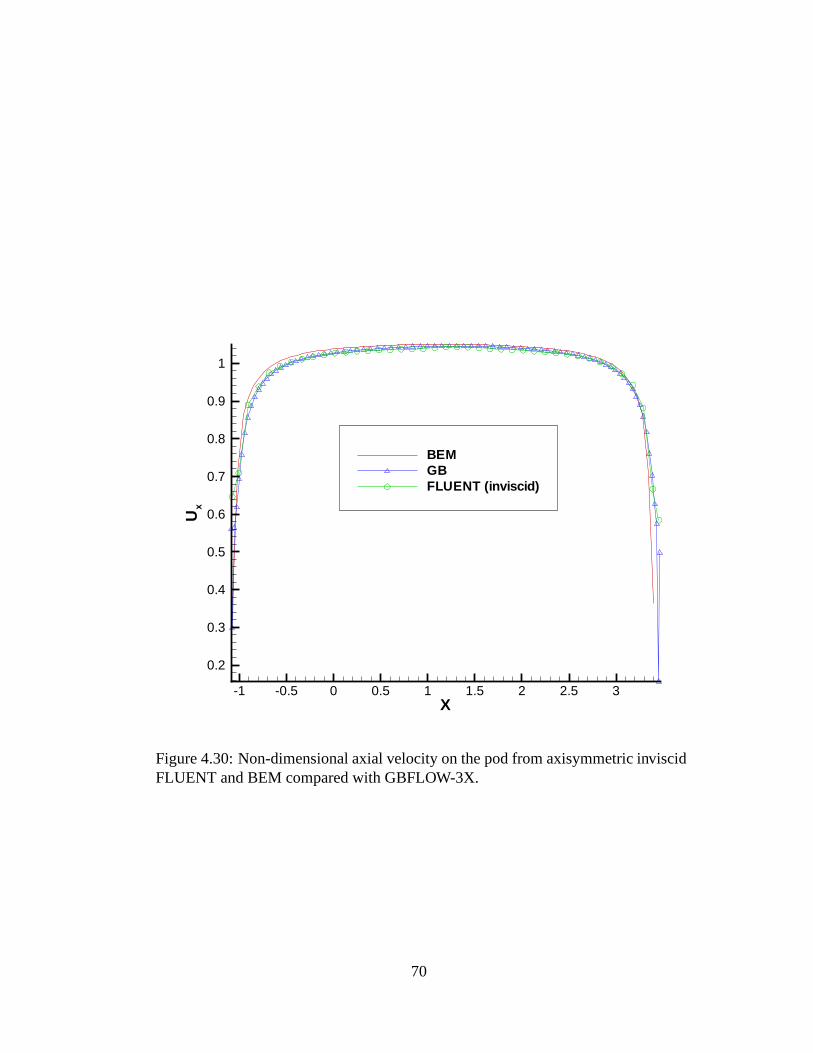
X
Ux
-1 -0.5 0 0.5 1 1.5 2 2.5 3
0.2
0.3
0.4
0.5
0.6
0.7
0.8
0.9
1
BEMGBFLUENT (inviscid)
Figure 4.30: Non-dimensional axial velocity on the pod from axisymmetric inviscidFLUENT and BEM compared with GBFLOW-3X.
70
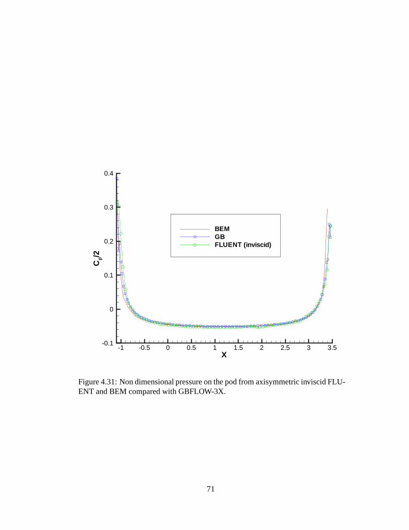
X
Cp/
2
-1 -0.5 0 0.5 1 1.5 2 2.5 3 3.5-0.1
0
0.1
0.2
0.3
0.4
BEMGBFLUENT (inviscid)
Figure 4.31: Non dimensional pressure on the pod from axisymmetric inviscid FLU-ENT and BEM compared with GBFLOW-3X.
71

Chapter 5
Axisymmetric Pod and Propeller Interaction
In the previous Chapter, the flow around an axisymmetric pod was determined in
the absence of a propeller. It is important to also know the flow, as well as the force
on the pod, in the presence of a propeller. Moreover, the presence of the pod alters
the inflow to the propeller and changes its performance characteristics. This Chapter
focuses on the pod and propeller interaction. Coupling between the VLM and the
FVM is carried out as detailed in Chapter 3. The axisymmetric version of FLUENT
will only be used in this chapter, i.e. the effects of the strut will be ignored. However,
the axisymmetric (GBFLOW-3X) as well as the 3-D (GBFLOW-3D) versions of the
Euler solver will be used. In this way the effects of the strut on the overall flow can
be estimated.
5.1 Experiment
In order to validate the method thoroughly, it is essential to apply it to realistic
geometries for which experimental data is available. One such experiment was done
by [Szantyr 2001a]. A comparison with the experimental work has been presented
in [Hsin et al. 2002], where the flow past a podded propulsor has been calculated
72

using both the boundary element method (applied to both the propeller and the pod)
and a coupled viscous/potential flow solver.
5.1.1 Experimental Setup
The experiments with the podded propulsor were performed in the cavitation tunnel
of the Technical University of Gdansk. The podded propulsor is placed on a spe-
cially developed experimental stand. The stand is fitted with a tensometric dynamo-
meter, enabling it to measure the longitudinal and the transverse components of
force, and the moment component about the vertical axis. The forces and moments
were measured in a coordinate system linked to the pod. The propulsor model is
made of glass-reinforced plastic. The entire stand is mounted on top of the tunnel
measuring section such that it could be rotated around the vertical axis. The forces
were measured for a pulling propeller and for twin rotating propellers with the inflow
at various yaw angles.
The principal dimensions of the pod used are presented below. More details on the
exact geometry of the pod and the strut are given in Appendix A.
• Length of podded propulsor : 412 mm
• Maximum pod diameter: 74 mm
• Diameter at each propeller location: 64 mm
• Length of the strut: 140 mm
• Chord of the strut: 109 mm
• Maximum thickness of the strut: 47 mm
73

The propeller used were modified KCA 110, chosen from the series presented by
[Gawn and Burrill 1957]. The propeller details are presented below.
• Propeller KCA 110 (modified) Gawn-Burrill series
• Propeller diameter for both propellers: 182 mm
• No. of blades: 3
• Blade area ratio of propeller A/A0: 0.8
• Pitch of pulling propeller (radially constant)P/D: 0.8
• Pitch of pushing propeller (radially constant) P/D: 1.108
All dimensions are made non-dimensional with respect to the radius of the propeller.
The detailed propeller geometries are given in Appendix A.
5.2 Propeller Configurations
The various podded propeller configurations that are solved using the present method
are:
• Pull type: The propeller is located in front of the strut and can be viewed as if
it is pulling the ship.
• Push type: The propeller is located aft of the strut, and it seems to push the
ship.
74

• Twin rotating type : Two propellers rotating in the same direction, both placed
either in front or aft of the strut, or, one propeller in front of the strut, and one
aft of it.
5.3 Pull Type
In a pull type podded propeller, the propeller is placed in front of the strut, which
joins the pod to the hull. The flow passes through the propeller before it passes over
the strut. Since the propeller is in front of the strut, it seems as if the propeller is
pulling the unit, and hence the name. Pull type podded propulsors are also called
pre-swirl podded propulsors. In this case there is no strut, but the propeller location
is similar to what it would be in the presence of a strut as shown in Figure 1.1.
5.3.1 Coupling with GBFLOW-3X
Initially, GBFLOW-3X is used to solve the pod and propeller problem. The axial
body force for Js = 0.5 and the effective wake location for a pull type configuration
are shown in Figure 5.1. Note that all components of body force are considered in
the calculations. A close-up of the body force is shown in Figure 5.2. It is obtained
after integration of pressures on the propeller obtained from MPUF-3A as mentioned
in Section 3.6.
Iterations are carried out between the methods (VLM and FVM) until a converged
solution is obtained. Figures 5.3 and 5.4 show the converged velocity and pres-
sure field contours around the pod, respectively. As can be seen the axial veloc-
ity increases as it passes the propeller and the flow seems to be sucked in. The
75
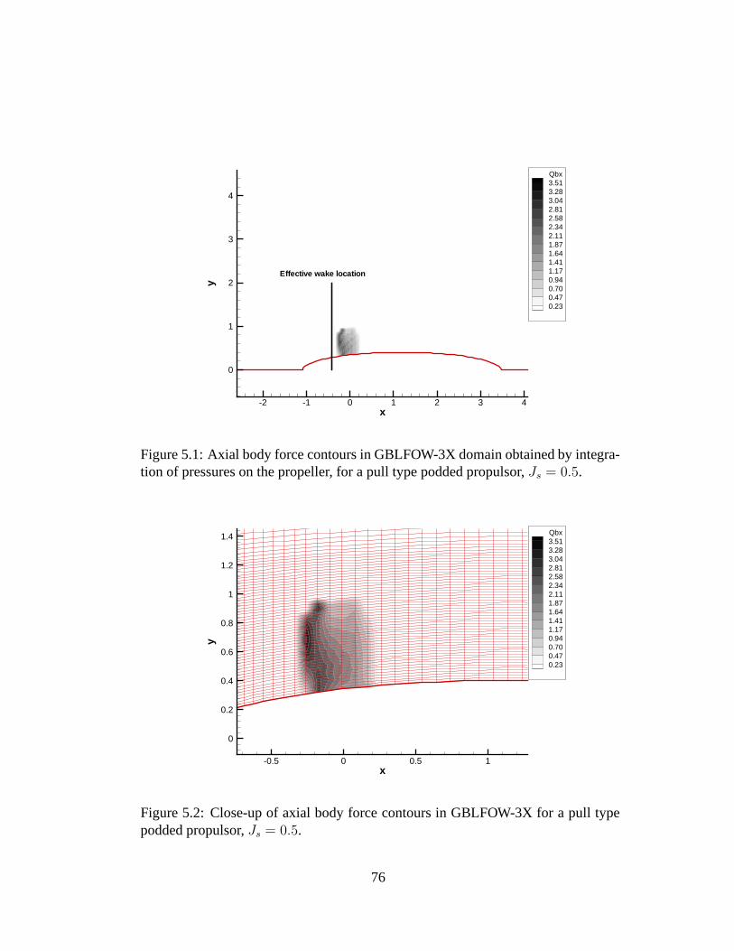
x
y
-2 -1 0 1 2 3 4
0
1
2
3
4
Qbx3.513.283.042.812.582.342.111.871.641.411.170.940.700.470.23
Effective wake location
Figure 5.1: Axial body force contours in GBLFOW-3X domain obtained by integra-tion of pressures on the propeller, for a pull type podded propulsor, Js = 0.5.
x
y
-0.5 0 0.5 1
0
0.2
0.4
0.6
0.8
1
1.2
1.4 Qbx3.513.283.042.812.582.342.111.871.641.411.170.940.700.470.23
Figure 5.2: Close-up of axial body force contours in GBLFOW-3X for a pull typepodded propulsor, Js = 0.5.
76

x
y
-2 0 2 4 6
0
1
2
3
4
5 u1.631.481.341.201.050.910.770.620.480.340.190.05
-0.09-0.24-0.38
Figure 5.3: Axial velocity contour in GBFLOW-3X for pull type podded propulsor,Js = 0.5
x
y
-2 0 2 4 6
0
1
2
3
4
5 p0.16
-0.02-0.19-0.36-0.54-0.71-0.88-1.06-1.23-1.40-1.58-1.75-1.92-2.10-2.27
Figure 5.4: Pressure contour in GBFLOW-3X for pull type podded propulsor, Js =0.5
77

R
100Γ
0.4 0.5 0.6 0.7 0.8 0.9-1.3
-1.2
-1.1
-1
-0.9
-0.8
-0.7
-0.6
-0.5
-0.4
-0.3
-0.2
-0.1
0
0th iter1st iter2nd iter3rd iter4th iter
Figure 5.5: Convergence of circulation distribution with iterations for GBFLOW-3Xcoupled with MPUF-3A, for pull type podded propulsor, Js = 0.5
convergence of circulation distribution with iterations is shown in Figure 5.5. The
circulation Γ, out of MPUF-3A is non-dimensionalised as,
Γnon−dim =Γ × 102
2πRVs
(5.1)
where, γ is the strength of the bound vortices in MPUF-3A.
Force Calculations
To get the total force on the pod, strut and the propeller system, the individual forces
have to be added keeping in mind the direction of forces. The pictorial representation
of the forces for 00 yaw angle is shown in Figure 5.6. The propeller thrust Fprop is
given in the negativeX direction while the force from GBFLOW and FLUENT is in
the positive X direction. The frictional force acting on the pod (and strut in the 3-D
78
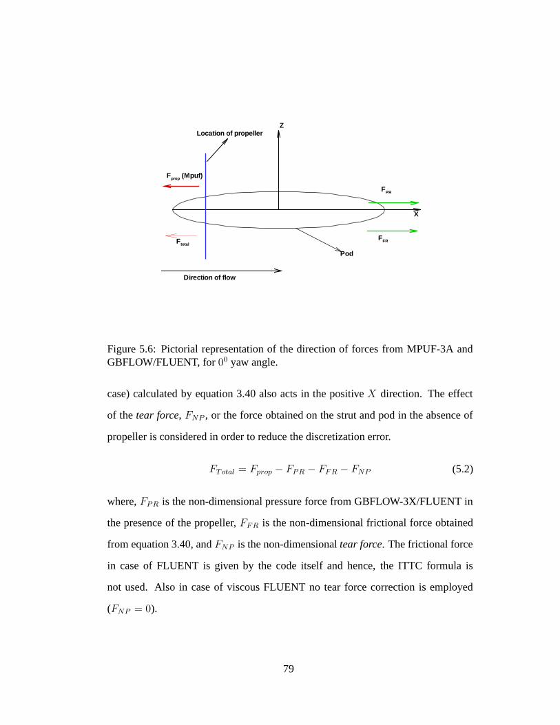
Z
X
Fprop (Mpuf)
Location of propeller
Direction of flow
FPR
Pod
FFRFtotal
Figure 5.6: Pictorial representation of the direction of forces from MPUF-3A andGBFLOW/FLUENT, for 00 yaw angle.
case) calculated by equation 3.40 also acts in the positive X direction. The effect
of the tear force, FNP , or the force obtained on the strut and pod in the absence of
propeller is considered in order to reduce the discretization error.
FTotal = Fprop − FPR − FFR − FNP (5.2)
where, FPR is the non-dimensional pressure force from GBFLOW-3X/FLUENT in
the presence of the propeller, FFR is the non-dimensional frictional force obtained
from equation 3.40, and FNP is the non-dimensional tear force. The frictional force
in case of FLUENT is given by the code itself and hence, the ITTC formula is
not used. Also in case of viscous FLUENT no tear force correction is employed
(FNP = 0).
79

Js
Fx
0.4 0.5 0.6 0.7 0.8 0.90
0.02
0.04
0.06
0.08
0.1
0.12
0.14
0.16
0.18
0.2
ExperimentalGB3X-MPUF
Figure 5.7: Comparison of axial force for a pulling propeller from the presentmethod compared with the measurements of [Szantyr 2001a].
Results
Runs for force calculations are carried out for four different advance ratios Js. Figure
5.7 shows the comparison of the total axial force calculated for a pulling propeller
from the numerical method (GBFLOW-3X/MPUF-3A) with that measured in the
experiments performed by [Szantyr 2001a]. Comparison of these two is not entirely
correct as the measurements are for a pod with a strut. The effects of the strut
can also be included by coupling GBFLOW-3D with MPUF-3A and the results are
shown in Figure 5.7. The break-up of non-dimensional forces from MPUF-3A and
GBFLOW-3X are shown in Table 5.1. The forces from GBFLOW-3X are modified
according to equation 3.39, so that they are non-dimensionalized the same way as
the forces from MPUF-3A and from [Szantyr 2001a].
80
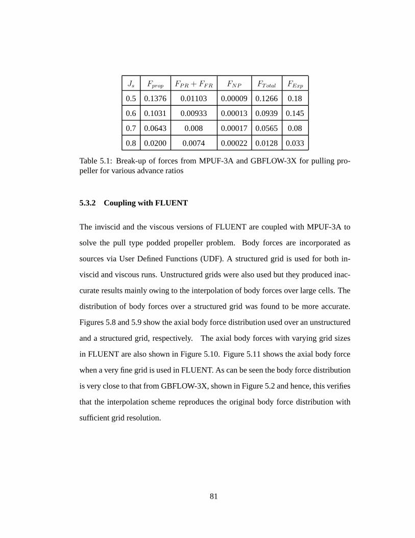
Js Fprop FPR + FFR FNP FTotal FExp
0.5 0.1376 0.01103 0.00009 0.1266 0.18
0.6 0.1031 0.00933 0.00013 0.0939 0.145
0.7 0.0643 0.008 0.00017 0.0565 0.08
0.8 0.0200 0.0074 0.00022 0.0128 0.033
Table 5.1: Break-up of forces from MPUF-3A and GBFLOW-3X for pulling pro-peller for various advance ratios
5.3.2 Coupling with FLUENT
The inviscid and the viscous versions of FLUENT are coupled with MPUF-3A to
solve the pull type podded propeller problem. Body forces are incorporated as
sources via User Defined Functions (UDF). A structured grid is used for both in-
viscid and viscous runs. Unstructured grids were also used but they produced inac-
curate results mainly owing to the interpolation of body forces over large cells. The
distribution of body forces over a structured grid was found to be more accurate.
Figures 5.8 and 5.9 show the axial body force distribution used over an unstructured
and a structured grid, respectively. The axial body forces with varying grid sizes
in FLUENT are also shown in Figure 5.10. Figure 5.11 shows the axial body force
when a very fine grid is used in FLUENT. As can be seen the body force distribution
is very close to that from GBFLOW-3X, shown in Figure 5.2 and hence, this verifies
that the interpolation scheme reproduces the original body force distribution with
sufficient grid resolution.
81

X
Y
-0.5 0 0.5 1
-0.2
0
0.2
0.4
0.6
0.8
1
1.2
1.4
3.513.283.042.812.572.342.101.871.641.401.170.930.700.460.23
Figure 5.8: Axial body force distribution in FLUENT for an unstructured grid, Js =0.5
X
Y
-0.5 0 0.5 1
-0.2
0
0.2
0.4
0.6
0.8
1
1.2
1.4
3.513.283.042.812.572.342.101.871.641.401.170.930.700.460.23
Figure 5.9: Axial body force distribution in FLUENT for a structured grid, Js = 0.5
82
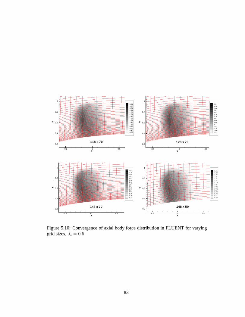
X
Y
-0.5 0 0.5
0.2
0.4
0.6
0.8
13.513.283.042.812.572.342.101.871.641.401.170.930.700.460.23
118 x 70
X
Y
-0.5 0 0.5
0.2
0.4
0.6
0.8
13.513.283.042.812.572.342.101.871.641.401.170.930.700.460.23
128 x 70
X
Y
-0.5 0 0.5
0.2
0.4
0.6
0.8
13.513.283.042.812.572.342.101.871.641.401.170.930.700.460.23
148 x 70
X
Y
-0.5 0 0.5
0.2
0.4
0.6
0.8
13.513.283.042.812.572.342.101.871.641.401.170.930.700.460.23
148 x 50
Figure 5.10: Convergence of axial body force distribution in FLUENT for varyinggrid sizes, Js = 0.5
83

x
y
-0.5 0 0.5 1
0
0.2
0.4
0.6
0.8
1
1.2
1.43.513.283.042.812.582.342.111.871.641.411.170.940.700.470.23
Figure 5.11: Axial body force distribution in FLUENT over a very fine structuredgrid, Js = 0.5
Inviscid case
Inviscid FLUENT is run with the same parameters as in Table 4.2 and with the source
terms included. Figures 5.12 and 5.13 show the converged velocity and pressure field
contour around the pod. The comparison of converged circulation distributions
from GBFLOW-3X and FLUENT (inviscid) is shown in Figure 5.14. It can be
seen that they agree very well. Figure 5.15 shows the comparison of the total axial
force calculated for a pulling propeller from FLUENT and from GBFLOW-3X. The
break-up of the forces is shown in Table 5.2.
84
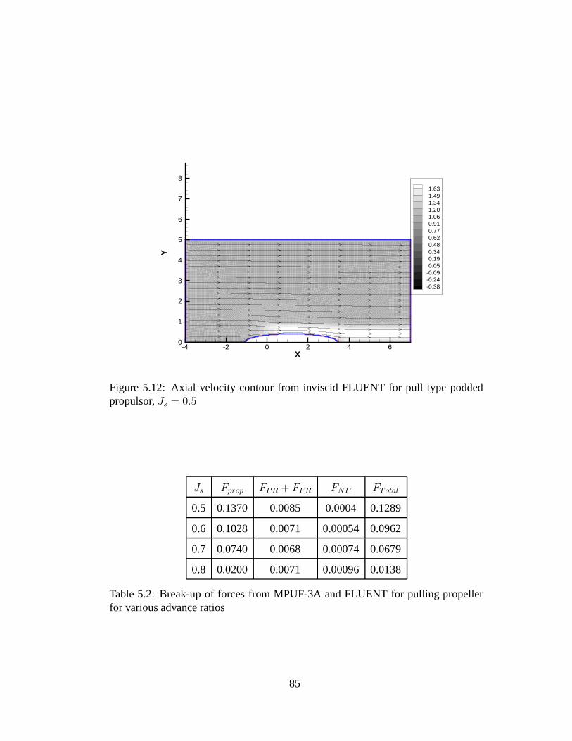
X
Y
3 4 5 6 7-0.6
-0.4
-0.2
0
0.2
0.4
0.6
0.8
1
1.2
Viscous FLUENT
X
Y
-4 -2 0 2 4 60
1
2
3
4
5
6
7
8
1.631.491.341.201.060.910.770.620.480.340.190.05
-0.09-0.24-0.38
Figure 5.12: Axial velocity contour from inviscid FLUENT for pull type poddedpropulsor, Js = 0.5
Js Fprop FPR + FFR FNP FTotal
0.5 0.1370 0.0085 0.0004 0.1289
0.6 0.1028 0.0071 0.00054 0.0962
0.7 0.0740 0.0068 0.00074 0.0679
0.8 0.0200 0.0071 0.00096 0.0138
Table 5.2: Break-up of forces from MPUF-3A and FLUENT for pulling propellerfor various advance ratios
85
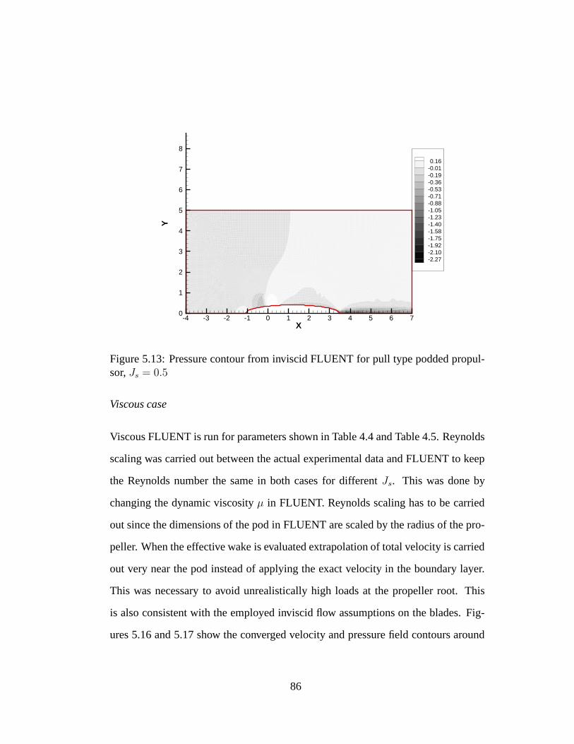
X
Y
3 4 5 6 7-0.6
-0.4
-0.2
0
0.2
0.4
0.6
0.8
1
1.2
Viscous FLUENT
X
Y
-4 -3 -2 -1 0 1 2 3 4 5 6 70
1
2
3
4
5
6
7
8
0.16-0.01-0.19-0.36-0.53-0.71-0.88-1.05-1.23-1.40-1.58-1.75-1.92-2.10-2.27
Figure 5.13: Pressure contour from inviscid FLUENT for pull type podded propul-sor, Js = 0.5
Viscous case
Viscous FLUENT is run for parameters shown in Table 4.4 and Table 4.5. Reynolds
scaling was carried out between the actual experimental data and FLUENT to keep
the Reynolds number the same in both cases for different Js. This was done by
changing the dynamic viscosity µ in FLUENT. Reynolds scaling has to be carried
out since the dimensions of the pod in FLUENT are scaled by the radius of the pro-
peller. When the effective wake is evaluated extrapolation of total velocity is carried
out very near the pod instead of applying the exact velocity in the boundary layer.
This was necessary to avoid unrealistically high loads at the propeller root. This
is also consistent with the employed inviscid flow assumptions on the blades. Fig-
ures 5.16 and 5.17 show the converged velocity and pressure field contours around
86

R
100Γ
0.4 0.5 0.6 0.7 0.8 0.9
-1.2
-1.1
-1
-0.9
-0.8
-0.7
-0.6
-0.5
-0.4
-0.3
-0.2
-0.1
0
FLUENT (inviscid)GBFLOW-3X
Figure 5.14: Comparison of converged circulation distributions predicted fromGBFLOW-3X and FLUENT(inviscid) coupled with MPUF-3A, for pull type pod-ded propulsor, Js = 0.5
87
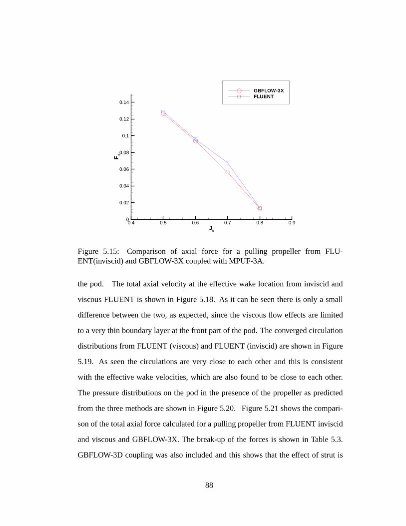
Js
Fx
0.4 0.5 0.6 0.7 0.8 0.90
0.02
0.04
0.06
0.08
0.1
0.12
0.14
GBFLOW-3XFLUENT
Figure 5.15: Comparison of axial force for a pulling propeller from FLU-ENT(inviscid) and GBFLOW-3X coupled with MPUF-3A.
the pod. The total axial velocity at the effective wake location from inviscid and
viscous FLUENT is shown in Figure 5.18. As it can be seen there is only a small
difference between the two, as expected, since the viscous flow effects are limited
to a very thin boundary layer at the front part of the pod. The converged circulation
distributions from FLUENT (viscous) and FLUENT (inviscid) are shown in Figure
5.19. As seen the circulations are very close to each other and this is consistent
with the effective wake velocities, which are also found to be close to each other.
The pressure distributions on the pod in the presence of the propeller as predicted
from the three methods are shown in Figure 5.20. Figure 5.21 shows the compari-
son of the total axial force calculated for a pulling propeller from FLUENT inviscid
and viscous and GBFLOW-3X. The break-up of the forces is shown in Table 5.3.
GBFLOW-3D coupling was also included and this shows that the effect of strut is
88

X
Y
-4 -2 0 2 4 60
1
2
3
4
5
6
7
8
1.631.491.341.201.060.910.770.620.480.340.190.05
-0.09-0.24-0.38
Figure 5.16: Axial velocity contour in viscous FLUENT for pull type poddedpropulsor, Js = 0.5, Re = 6.26 × 10⁵
not very significant in this case. Also, including the effects of viscosity did not seem
to improve the correlation with experiments. The reasons for the discrepancyof the
results from all the methods with the measurements especially at lower Js are not
known at this point.
Similar to the results shown in Figure 4.25, runs were carried out using the RSM
model in FLUENT and compared to those from the k− ε model. The fore propeller
was present and comparisons were carried out at the aft effective wake location be-
tween the axial and swirl velocities. Figures 5.22 and 5.23 show this comparison.
It can be seen that the velocities from the RSM model are much closer (except very
close to the pod) to the inviscid result, as expected, and hence this model is used for
all future runs. The k − ε model, as already discussed in Section 4.2.4, appears to
over diffuse the flow vorticity.
89

X
Y
0 50
1
2
3
4
5
6
7
8
0.16-0.01-0.19-0.36-0.53-0.71-0.88-1.05-1.23-1.40-1.58-1.75-1.92-2.10-2.27
Figure 5.17: Pressure contour in viscous FLUENT for pull type podded propulsor,Js = 0.5, Re = 6.26 × 10⁵
Js Fprop FPR + FFR FTotal
0.5 0.1371 0.0057 0.1314
0.6 0.1031 0.0061 0.0970
0.7 0.0646 0.0049 0.0597
0.8 0.0202 0.0051 0.0151
Table 5.3: Break-up of forces from MPUF-3A and viscous FLUENT for pullingpropeller for various advance ratios
90

Ux
Y
0 0.5 1 1.5
0.5
1
1.5
FLUENT (inviscid)FLUENT (viscous)
Figure 5.18: Total axial velocity at effective wake location for viscous and inviscidFLUENT coupled with MPUF-3A, for pull type podded propulsor, Js = 0.5, Re =6.26 × 10⁵
91

R
100Γ
0.4 0.5 0.6 0.7 0.8 0.9 1-1.3
-1.2
-1.1
-1
-0.9
-0.8
-0.7
-0.6
-0.5
-0.4
-0.3
-0.2
-0.1
0
FLUENT(inviscid)FLUENT (viscous)
Figure 5.19: Converged circulation distributions predicted from FLUENT (viscous)and FLUENT(inviscid) coupled with MPUF-3A, for pull type podded propulsor,Js = 0.5, Re = 6.26 × 10⁵
92

X
Cp
-1 0 1 2 3
-2.5
-2
-1.5
-1
-0.5
0
0.5
GBFLOW-3XFLUENT (inviscid)FLUENT (viscous)
Figure 5.20: Converged pressure distributions predicted from GBFLOW-3X, FLU-ENT (viscous) and FLUENT(inviscid) coupled with MPUF-3A, for pull type pod-ded propulsor, Js = 0.5, Re = 6.26 × 10⁵
93

Js
Fx
0.4 0.5 0.6 0.7 0.8 0.90
0.02
0.04
0.06
0.08
0.1
0.12
0.14
0.16
0.18
0.2
ExperimentalGBFLOW-3XFLUENT (inviscid)GBFLOW-3DFLUENT (viscous)
Figure 5.21: Comparison of axial force for a pulling propeller from FLU-ENT(inviscid & viscous) and GBFLOW coupled with MPUF-3A.
94
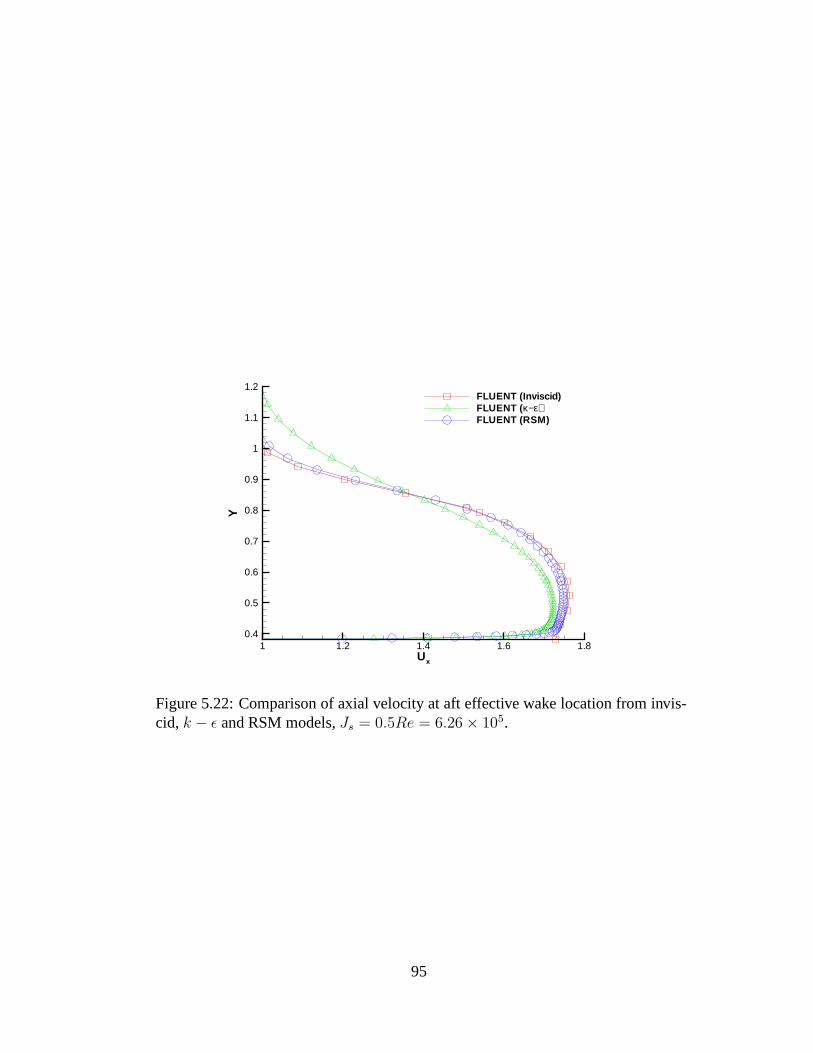
Ux
Y
1 1.2 1.4 1.6 1.80.4
0.5
0.6
0.7
0.8
0.9
1
1.1
1.2FLUENT (Inviscid)FLUENT (κ−ε)FLUENT (RSM)
Figure 5.22: Comparison of axial velocity at aft effective wake location from invis-cid, k − ε and RSM models, Js = 0.5Re = 6.26 × 10⁵.
95

Ux
Y
0 0.1 0.2 0.3 0.4 0.50.4
0.6
0.8
1
1.2FLUENT (Inviscid)FLUENT (κ−ε)FLUENT (RSM)
Figure 5.23: Comparison of swirl velocity at aft effective wake location from invis-cid, k − ε and RSM models, Js = 0.5Re = 6.26 × 10⁵.
96

5.4 Push Type
In a push type podded propulsor the propeller is placed aft of the strut. The flow
passes the strut before it reaches the propeller. Since we will use axisymmetric flow
solvers the effect of the strut will be ignored. GBFLOW-3D has also been coupled
with MPUF-3A and the effects of the strut on the solution can be estimated. The
propeller and effective wake locations are as shown in Figure 4.23.
5.4.1 Coupling with GBFLOW-3X
Again, GBFLOW-3X is used initially to solve the push type unit in inviscid flow.
The body force distribution for the push type propeller (for Js = 0.5) is shown in
Figure 5.24. Figures 5.25 and 5.26 show the converged velocity and pressure field
x
y
2 2.5 3 3.5
0
0.2
0.4
0.6
0.8
1
1.2
1.4
1.6
Qbx6.876.235.584.944.293.653.002.361.721.070.43
-0.22-0.86-1.51-2.15
Figure 5.24: Body force contours in GBLFOW-3X domain obtained by integrationof pressures on the propeller, for a push type podded propulsor, Js = 0.5.
97

x
y
0 50
1
2
3
4
5
6
7
8u
2.272.051.831.611.391.170.950.730.520.300.08
-0.14-0.36-0.58-0.80
Figure 5.25: Axial velocity contour in GBFLOW-3X for push type podded propul-sor, Js = 0.5
contour around the pod. The convergence of circulation distribution with iterations
is shown in Figure 5.27. Force calculations are carried out for four different advance
ratios. The break-up of the non-dimensional forces from MPUF-3A and GBFLOW-
3X are shown in Table 5.4.
98

x
y
0 50
1
2
3
4
5
6
7
8p
0.190.03
-0.13-0.29-0.45-0.61-0.77-0.93-1.09-1.25-1.40-1.56-1.72-1.88-2.04
Figure 5.26: Pressure contour in GBFLOW-3X for push type podded propulsor,Js = 0.5
R
100Γ
0.4 0.5 0.6 0.7 0.8 0.9
-2.5
-2
-1.5
-1
-0.5
0
0th iter1st iter2nd iter3rd iter4th iter
Figure 5.27: Convergence of circulation distribution with iterations for GBFLOW-3X for push type podded propulsor, Js = 0.5
99

Js Fprop FPR + FFR FNP FTotal
0.5 0.2806 0.0233 0.00009 0.2572
0.6 0.2471 0.0234 0.00013 0.2236
0.7 0.2090 0.0218 0.00017 0.1871
0.8 0.1662 0.0192 0.00022 0.1468
Table 5.4: Break-up of forces from MPUF-3A and GBFLOW-3X for pushing pro-peller for various advance ratios
100

5.4.2 Coupling with FLUENT
Both the inviscid and viscous versions of FLUENT are used to solve the coupled
problem. Figures 5.28 and 5.29 show the body forces for the inviscid and viscous
runs.
X
Y
2 2.5 3 3.5
0
0.2
0.4
0.6
0.8
1
1.2
1.4
1.6
6.876.295.705.124.533.953.372.782.201.611.030.44
-0.14-0.72-1.31
Figure 5.28: Body force distribution in FLUENT on the grid for inviscid case, Js =0.5
Inviscid case
Inviscid FLUENT is run with the same parameters as for the pull type case. Figure
5.30 shows the axial velocity contour for this case. Next, comparisons are carried
out between GBFLOW-3X and FLUENT inviscid. Figure 5.31 shows the compari-
son of converged effective axial velocity at the effective wake location. As is seen
101

X
Y
2 2.5 3 3.5
0
0.2
0.4
0.6
0.8
1
1.2
1.4
1.6
6.876.295.705.124.533.953.372.782.201.611.030.44
-0.14-0.72-1.31
Figure 5.29: Body force distribution in FLUENT on the grid for viscous case, Js =0.5, Re = 6.26 × 10⁵
the effective axial velocity from both methods compare very well with each other.
The comparison of converged circulation distribution between GBFLOW-3X and
FLUENT (inviscid) is shown in Figure 5.32. Figure 5.33 shows the comparison of
the total axial force calculated for a pulling propeller from FLUENT (inviscid) and
from GBFLOW-3X. The break-up of the forces is shown in Table 5.5. We see that
results from GBFLOW-3X and the inviscid version of FLUENT are very close to
each other and this is a very strong indication that both methods are implemented
correctly. Nevertheless, a systematic grid dependence study is needed to verify the
two approaches fully.
102

X
Y
-4 -2 0 2 4 60
1
2
3
4
5
6
7
8
2.272.051.831.611.391.170.950.730.520.300.08
-0.14-0.36-0.58-0.80
Figure 5.30: Axial velocity contour in inviscid FLUENT for push type poddedpropulsor, Js = 0.5
Js Fprop FPR + FFR FNP FTotal
0.5 0.279 0.024 0.0004 0.2546
0.6 0.2474 0.021 0.00054 0.2259
0.7 0.2106 0.018 0.00074 0.1918
0.8 0.1693 0.015 0.00096 0.1533
Table 5.5: Break-up of forces from MPUF-3A and inviscid FLUENT for pushingpropeller for various advance ratios
103

Ux
Y
0 0.2 0.4 0.6 0.8 1 1.2 1.4 1.6 1.8
0.5
0.75
1
GBFLOW-3XFLUENT (inviscid)
Figure 5.31: Comparison of effective axial velocity between GBFLOW-3X andFLUENT (inviscid) coupled with MPUF-3A, for a push type unit, Js = 0.5.
104

R
100Γ
0.4 0.5 0.6 0.7 0.8 0.9-2.4
-2.3
-2.2
-2.1
-2
-1.9
-1.8
-1.7
-1.6
-1.5
-1.4
-1.3
-1.2
-1.1
FLUENT (inviscid)GBFLOW-3X
Figure 5.32: Converged circulation distributions predicted from GBFLOW-3X andFLUENT(inviscid) coupled with MPUF-3A, for push type podded propulsor, Js =0.5
105

Js
Fx
0.4 0.5 0.6 0.7 0.8 0.90
0.05
0.1
0.15
0.2
0.25
0.3
0.35
0.4
Fluent (Inviscid)GBFLOW-3X
Figure 5.33: Axial force for a pushing propeller predicted from FLUENT (inviscid)and GBFLOW-3X coupled with MPUF-3A.
106

X
Y
-4 -2 0 2 4 60
1
2
3
4
5
6
7
8
2.272.051.831.611.391.170.950.730.520.300.08
-0.14-0.36-0.58-0.80
Figure 5.34: Axial velocity contours predicted by viscous FLUENT for push typepodded propulsor, Js = 0.5, Re = 6.26 × 10⁵
Viscous Case
Viscous FLUENT is run for the same parameters as for the pull type case except now
by using the RSM turbulence model. Figure 5.34 shows the axial velocity contour
from the viscous solver. The total axial velocity at the effective wake plane location
from inviscid and viscous FLUENT is compared next in Figure 5.35. The effective
wakes are also compared in Figure 5.36. It can be seen that the velocity in the
viscous case is lower due to onset of viscous effects. The circulation distributions
obtained from inviscid and viscous FLUENT are compared in Figure 5.37. Figure
5.39 shows the comparison of the total axial force calculated for a pulling propeller
from FLUENT (inviscid and viscous) and from GBFLOW-3X. The break-up of the
forces is shown in Table 5.6. The lower effective velocity in the viscous case results
107

Ux
Y
0 0.5 1 1.50.4
0.5
0.6
0.7
0.8
0.9
1
1.1
1.2
1.3
1.4
1.5
FLUENT (inviscid)FLUENT (RSM)
Figure 5.35: Comparison of total axial velocity at effective wake plane location frominviscid and viscous FLUENT coupled with MPUF-3A, Js = 0.5, Re = 6.26 × 10⁵
in higher circulation and hence higher forces. Figure 5.38 also shows the pressure
distribution along the body obtained from the different methods. As expected the
GBFLOW-3X and inviscid FLUENT solutions are close to each other. In the case
of the presence of the strut the flow will change significantly for the push type unit.
The velocity from the viscous solver should be considerably lower at the top of the
propeller disk due to the viscous losses at the strut. Comparisons are not carried out
with experiments as no measurements were available for this type of propulsor.
108

Ux
Y
0 0.2 0.4 0.6 0.8 1 1.2 1.4 1.6 1.8
0.4
0.6
0.8
1 FLUENT (inviscid)
FLUENT-RSM
Figure 5.36: Comparison of effective velocity at effective wake plane location frominviscid and viscous FLUENT coupled with MPUF-3A, Js = 0.5, Re = 6.26 × 10⁵
Js Fprop FPR + FFR FTotal
0.5 0.298 0.0255 0.2725
0.6 0.278 0.020 0.258
0.7 0.244 0.020 0.224
0.8 0.20 0.025 0.175
Table 5.6: Break-up of forces from MPUF-3A and viscous FLUENT for pushingpropeller for various advance ratios
109
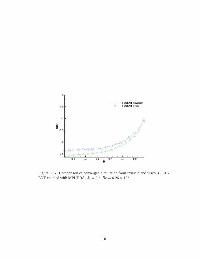
R
100Γ
0.4 0.5 0.6 0.7 0.8 0.9
-2.5
-2
-1.5
-1
-0.5
0
FLUENT (inviscid)FLUENT (RSM)
Figure 5.37: Comparison of converged circulation from inviscid and viscous FLU-ENT coupled with MPUF-3A, Js = 0.5, Re = 6.26 × 10⁵
110

X
Cp
-1 0 1 2 3-4
-3
-2
-1
0
FLUENT (RSM)GBFLOW-3XFLUENT (INVISCID)
Figure 5.38: Comparison of pressure distributions along the body for a pushing pro-peller from FLUENT(inviscid & viscous) and GBFLOW-3X coupled with MPUF-3A.
111
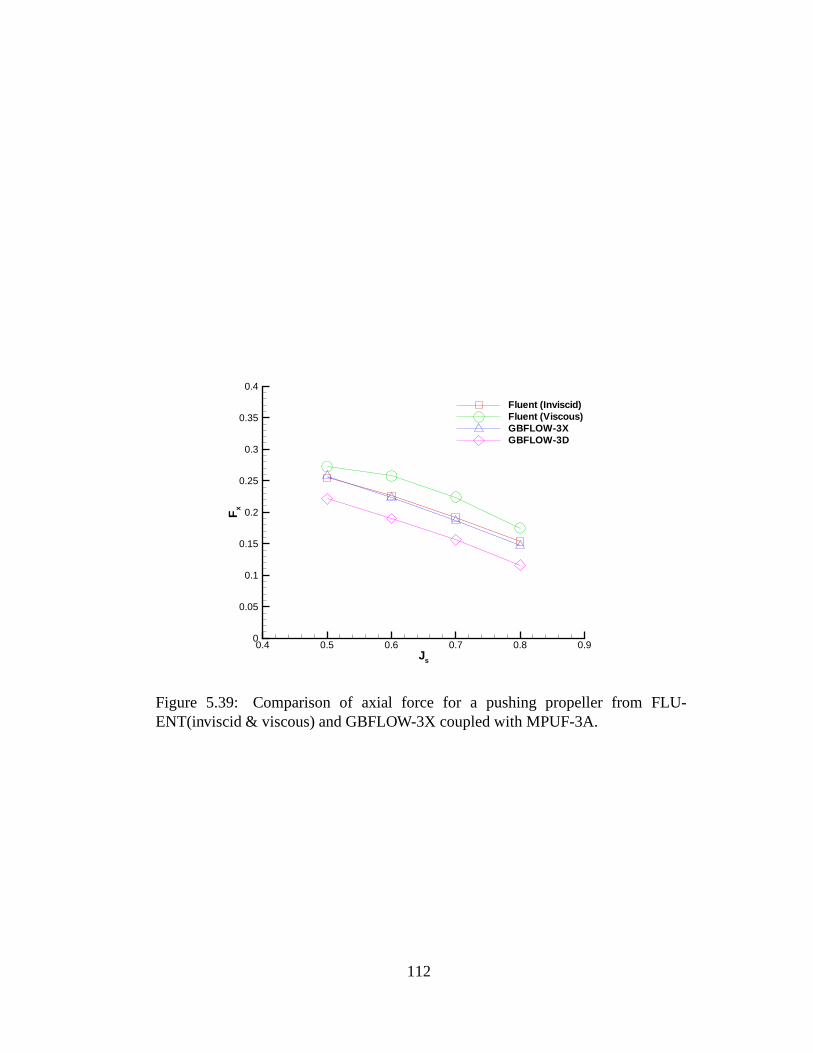
Js
Fx
0.4 0.5 0.6 0.7 0.8 0.90
0.05
0.1
0.15
0.2
0.25
0.3
0.35
0.4
Fluent (Inviscid)Fluent (Viscous)GBFLOW-3XGBFLOW-3D
Figure 5.39: Comparison of axial force for a pushing propeller from FLU-ENT(inviscid & viscous) and GBFLOW-3X coupled with MPUF-3A.
112

5.5 Twin type
In this case there are two propellers each at the fore and aft propeller location. The
flow to the aft propeller is modified by the fore propeller. In this case both pro-
pellers are left handed. So unlike the case of a contra-rotating system there is no
cancellation of swirl downstream of the aft propeller.
5.5.1 Coupling of GBFLOW-3X
GBFLOW-3X is coupled with MPUF-3A to solve the twin type propulsor problem.
The interaction between both the propellers and the pod is taken into account by
solving each propeller individually and by including the body forces from both in
GBFLOW-3X. Figures 5.40 and 5.41 show the axial velocity and the pressure con-
tours around the pod in presence of the propellers. The convergence of circulation
distribution for fore and aft propeller are shown in Figures 5.42 and 5.43. Runs for
force calculations are carried out for four different advance ratios Js. Figure 5.44
shows the comparison of the total axial force calculated for a twin type propeller
unit using the numerical method, with that measured in the experiments performed
by [Szantyr 2001a]. Comparison of these two is not entirely correct as explained
for the pull type case. The break-up of non-dimensional forces from MPUF-3A and
GBFLOW-3X are shown in Table 5.7.
113

x
y
0 50
1
2
3
4
5
6
7
8u
2.151.951.741.541.341.130.930.730.520.320.12
-0.09-0.29-0.49-0.70
Figure 5.40: Axial velocity contour in GBFLOW-3X for twin type podded propulsor,Js = 0.5
x
y
0 50
1
2
3
4
5
6
7
8p
0.200.05
-0.10-0.25-0.41-0.56-0.71-0.86-1.01-1.16-1.31-1.46-1.61-1.76-1.92
Figure 5.41: Pressure contour in GBFLOW-3X for twin type podded propulsor, Js =0.5
114

R
100Γ
0.4 0.5 0.6 0.7 0.8 0.9-1.3
-1.2
-1.1
-1
-0.9
-0.8
-0.7
-0.6
-0.5
-0.4
-0.3
-0.2
-0.1
00th iter1st iter2nd iter3rd iter
Figure 5.42: Convergence of circulation distribution with iterations for fore propellerfrom GBFLOW-3X for twin type podded propulsor, Js = 0.5
Js Fpropf Fpropa FPR + FFR FNP FTotal
0.5 0.1355 0.1477 0.02628 0.00009 0.257
0.6 0.1009 0.1428 0.02522 0.00013 0.2186
0.7 0.0618 0.1394 0.0242 0.00017 0.1764
0.8 0.0161 0.1400 0.0231 0.00022 0.1332
Table 5.7: Break-up of forces from MPUF-3A and GBFLOW-3X for twin propellerunit for various advance ratios
115
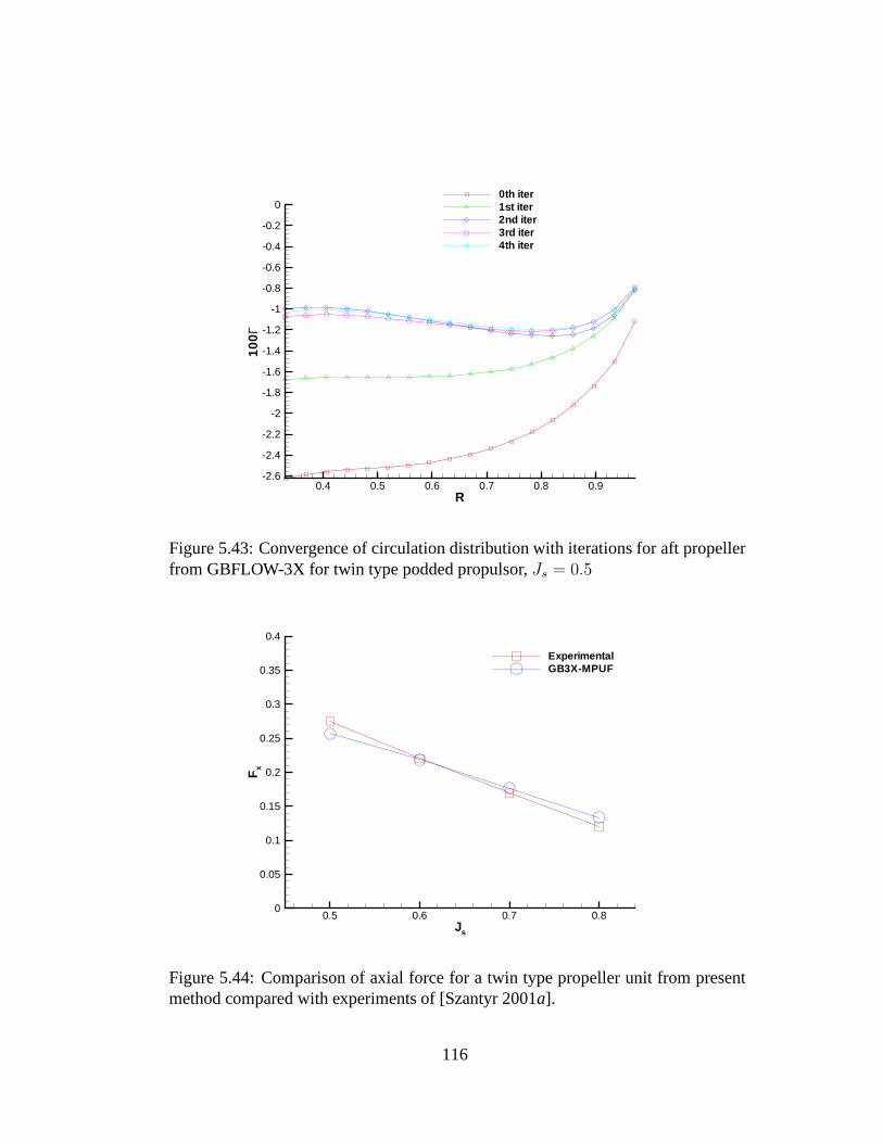
R
100Γ
0.4 0.5 0.6 0.7 0.8 0.9-2.6
-2.4
-2.2
-2
-1.8
-1.6
-1.4
-1.2
-1
-0.8
-0.6
-0.4
-0.2
00th iter1st iter2nd iter3rd iter4th iter
Figure 5.43: Convergence of circulation distribution with iterations for aft propellerfrom GBFLOW-3X for twin type podded propulsor, Js = 0.5
Js
Fx
0.5 0.6 0.7 0.80
0.05
0.1
0.15
0.2
0.25
0.3
0.35
0.4
ExperimentalGB3X-MPUF
Figure 5.44: Comparison of axial force for a twin type propeller unit from presentmethod compared with experiments of [Szantyr 2001a].
116
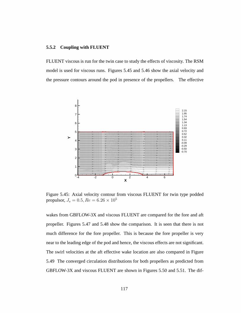
5.5.2 Coupling with FLUENT
FLUENT viscous is run for the twin case to study the effects of viscosity. The RSM
model is used for viscous runs. Figures 5.45 and 5.46 show the axial velocity and
the pressure contours around the pod in presence of the propellers. The effective
X
Y
-4 -2 0 2 4 60
1
2
3
4
5
6
7
8
2.151.951.741.541.341.130.930.720.520.320.11
-0.09-0.29-0.50-0.70
Figure 5.45: Axial velocity contour from viscous FLUENT for twin type poddedpropulsor, Js = 0.5, Re = 6.26 × 10⁵
wakes from GBFLOW-3X and viscous FLUENT are compared for the fore and aft
propeller. Figures 5.47 and 5.48 show the comparison. It is seen that there is not
much difference for the fore propeller. This is because the fore propeller is very
near to the leading edge of the pod and hence, the viscous effects are not significant.
The swirl velocities at the aft effective wake location are also compared in Figure
5.49 The converged circulation distributions for both propellers as predicted from
GBFLOW-3X and viscous FLUENT are shown in Figures 5.50 and 5.51. The dif-
117

X
Y
-2 0 2 4 6
0
1
2
3
4
5
60.200.05
-0.10-0.25-0.41-0.56-0.71-0.86-1.01-1.16-1.32-1.47-1.62-1.77-1.92
Figure 5.46: Pressure contour from viscous FLUENT for twin type podded propul-sor, Js = 0.5, Re = 6.26 × 10⁵
ference in the circulation distribution for the aft propeller can be attributed to the
difference in the swirl velocity component.
The break-up of non-dimensional forces from MPUF-3A and viscous FLUENT is
shown in Table 5.8. Figure 5.53 shows the comparison of the total axial force be-
tween GBFLOW-3X and viscous FLUENT. Also, the results from GBFLOW-3D are
somewhat higher. This is mainly because the flow to the aft propeller is changed due
to the presence of the strut, which reduces the effective velocity resulting in higher
circulation. Figure 5.52 shows the pressure distribution along the body obtained
from the different methods.
118

Ux
Y
0 0.1 0.2 0.3 0.4 0.5 0.6 0.7 0.8 0.9 1 1.1 1.2
0.4
0.5
0.6
0.7
0.8
0.9
1
1.1
FLUENT (RSM)
GBFLOW-3X
Figure 5.47: Comparison of effective velocity for fore propeller between GBFLOW-3X and FLUENT (viscous) coupled with MPUF-3A, for a twin type unit, Js =0.5, Re = 6.26 × 10⁵.
Js Fpropf Fpropa FPR + FFR FTotal
0.5 0.1349 0.1642 0.01122 0.2878
0.6 0.1004 0.1571 0.02236 0.2351
0.7 0.0616 0.1502 0.0195 0.1923
0.8 0.0164 0.1438 0.0177 0.1425
Table 5.8: Break-up of forces from MPUF-3A and FLUENT (RSM) for twin pro-peller unit for various advance ratios
119

Ux
Y
0 0.5 1 1.5
0.4
0.5
0.6
0.7
0.8
0.9
1
1.1
1.2
FLUENT (RSM)
GBFLOW-3X
Figure 5.48: Comparison of effective axial velocity for aft propeller predicted fromGBFLOW-3X and FLUENT (viscous) coupled with MPUF-3A, for a twin type unit,Js = 0.5, Re = 6.26 × 10⁵.
120

Ux
Y
0.1 0.2 0.3 0.4 0.5
0.4
0.5
0.6
0.7
0.8
0.9
1
1.1
1.2
FLUENT (RSM)
GBFLOW-3X
Figure 5.49: Comparison of effective swirl velocity for aft propeller predicted fromGBFLOW-3X and FLUENT (viscous) coupled with MPUF-3A, for a twin type unit,Js = 0.5, Re = 6.26 × 10⁵.
121

R
100Γ
0.4 0.5 0.6 0.7 0.8 0.9-1.3
-1.2
-1.1
-1
-0.9
-0.8
-0.7
-0.6
-0.5
-0.4
-0.3
-0.2
-0.1
0
FLUENT (RSM)GBFLOW-3X
Figure 5.50: Comparison of circulation distributions for fore propeller predictedfrom GBFLOW-3X and FLUENT (viscous) coupled with MPUF-3A, for a twin typeunit, Js = 0.5, Re = 6.26 × 10⁵.
122

R
100Γ
0.4 0.5 0.6 0.7 0.8 0.9-1.5
-1
-0.5
0FLUENT (RSM)GBFLOW-3X
Figure 5.51: Comparison of circulation distributions for aft propeller predicted fromGBFLOW-3X and FLUENT (viscous) coupled with MPUF-3A, for a twin type unit,Js = 0.5, Re = 6.26 × 10⁵.
123

X
Cp
-1 0 1 2 3-2
-1
0
1
FLUENT (RSM)GBFLOW-3X
Figure 5.52: Comparison of pressure distributions along the body for a twin pro-peller from FLUENT(viscous) and GBFLOW-3X coupled with MPUF-3A.
124

Js
Fx
0.4 0.5 0.6 0.7 0.8 0.90
0.05
0.1
0.15
0.2
0.25
0.3
0.35
0.4
ExperimentalGBFLOW-3XGBFLOW-3DFLUENT-RSM
Figure 5.53: Comparison of axial force for a twin type propeller unit fromGBFLOW-3X and viscous FLUENT coupled with MPUF-3A.
125

Chapter 6
Pod with strut
In this chapter, GBFLOW-3D, the fully 3-dimensional Euler solver is applied to
a pod with the strut and the results are compared with those from other methods
namely, the 3-D version of FLUENT and the three dimensional BEM. The existence
of the strut over the pod makes the problem fully 3-dimensional and non-symmetric
in nature. Convergence studies are carried out for all methods.
6.1 3-D Euler Solver (GBFLOW-3D)
In Chapter 4 an axi-symmetric pod was solved. But a real situation involves the
presence of a strut and a hull over the strut, which acts as a wall. The Euler solver
has to be capable of handling the interactions among the pod, the strut and the hull.
The wall boundary conditions are applied on the pod, strut and hull so that the flow
does not penetrate the body. A Finite Volume Method based Euler solver is applied
to solve the problem. [Kakar 2002]
126
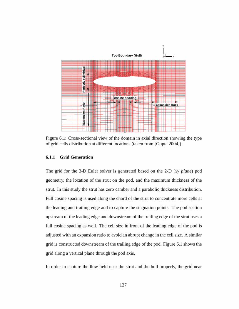
X
Y
ZTop Boundary (Hull)
cosine spacing
Per
fect
lycy
lind
rical
Expansion Ratio
Exp
ansi
onR
atio
Figure 6.1: Cross-sectional view of the domain in axial direction showing the typeof grid cells distribution at different locations (taken from [Gupta 2004]).
6.1.1 Grid Generation
The grid for the 3-D Euler solver is generated based on the 2-D (xy plane) pod
geometry, the location of the strut on the pod, and the maximum thickness of the
strut. In this study the strut has zero camber and a parabolic thickness distribution.
Full cosine spacing is used along the chord of the strut to concentrate more cells at
the leading and trailing edge and to capture the stagnation points. The pod section
upstream of the leading edge and downstream of the trailing edge of the strut uses a
full cosine spacing as well. The cell size in front of the leading edge of the pod is
adjusted with an expansion ratio to avoid an abrupt change in the cell size. A similar
grid is constructed downstream of the trailing edge of the pod. Figure 6.1 shows the
grid along a vertical plane through the pod axis.
In order to capture the flow field near the strut and the hull properly, the grid near
127

X
Y
Z
Top Boundary (Hull)
Pod
Strut
K=1K=2
K
Figure 6.2: Cross-sectional view of the domain showing the grid cells near the strutand the pod. Circumferential cells are uniformly distributed.
the strut has to be fairly dense, and the aspect ratio of the grid cells should be close
to one. Figure 6.2 shows the view of the strut in a plane along a station. To make
a uniform grid at the far stream boundary, with dense grid near the strut, a large
number of circumferential cells are required. One-fourth of the total circumferential
cells are placed on the hull, with three-fourths on the circular far stream domain. If
less cells are used, the grid points near the strut move away from the body, which
leads to inaccurate results. Large number of cells lead to increase in the run time.
Therefore, a grid like that shown in Figure 6.2 is chosen. The hull and far stream
is given the index j = Nj. An alternate grid arrangement is also used in which the
circumferential cells, index k, are clustered near the strut. Figure 6.3 shows this cell
arrangement.
128

Figure 6.3: Cross-sectional view of the domain showing the grid cells near the strutand the pod. Circumferential cells are clustered near the strut.
6.1.2 Boundary Conditions
The boundary conditions are applied as detailed in Section 3.2.3. The wall boundary
conditions are applied on the surface of the pod, strut and the hull. Free stream
boundary condition is applied at j = Nj, where the circumferential index k is
greater than (Nk − 1)/8 and less than 7(Nk − 1)/8. In the region j = Nj, k less
than (Nk−1)/8, and k greater than 7(Nk−1)/8 hull boundary condition is applied.
6.1.3 Results
Convergence studies are carried out for GBFLOW-3D. The flow field around the
body and the pressure force on the body is obtained. First, runs are carried out with
the grid having uniform circumferential cell distribution, but varying number of cells
in the axial direction. Velocity and pressure comparisons are carried out at a location
129

X
Y
Z
y=1.0
Figure 6.4: Location on strut where velocity and pressure comparisons are carriedout.
on the strut where it intersects the plane y=1.0. The location is shown in Figure 6.4.
Initially convergence studies are carried out by varying the number of nodes in the
axial direction. Runs were carried out for 101, 121 and 141 nodes in the axial direc-
tion over the whole domain. The axial velocity and pressure were compared at the
location y = 1.0. Figures 6.5 and 6.6 show the convergence with varying grid size
in the axial direction. Next, comparisons are carried out between the two different
types of grids used in the k direction, i.e. one uniformly distributed and the other
with cells clustered near the strut. The number of nodes in the circumferential direc-
tion is fixed to k = 121. Figures 6.7 and 6.8 show the comparison of axial velocity
and pressure, respectively, from the two grids. It will be seen (when comparisons are
carried out with FLUENT) that the results from the grid with cells clustered near the
strut are more accurate. It is also important to validate the solution obtained from
the new grid by carrying out convergence studies. Runs are carried out by varying
130

x
u
-0.5 0 0.5
0.4
0.5
0.6
0.7
0.8
0.9
1
1.1
1.2
1.3
1.4
1.5
101 x 50 x 65
121 x 50 x 65
141 x 50 x 65
Figure 6.5: Convergence of axial velocity with varying number of nodes in axialdirection in GBFLOW-3D.
x
p
-0.5 0 0.5
-0.2
-0.1
0
0.1
0.2
0.3
0.4
101 x 50 x 65
121 x 50 x 65
141 x 50 x 65
Figure 6.6: Convergence of pressure with varying number of nodes in axial directionin GBFLOW-3D.
131

x
u
-0.5 0 0.5
0.8
0.9
1
1.1
1.2
1.3
1.4
1.5
Uniform distribution
Clustered near strut
Figure 6.7: Comparison of axial velocity between the two different types of gridsused in k direction in GBFLOW-3D, k = 121
x
p
-0.5 0 0.5-0.4
-0.3
-0.2
-0.1
0
0.1
0.2
0.3
0.4
Uniform distribution
Clustered near strut
Figure 6.8: Comparison of pressure between the two different types of grids used ink direction in GBFLOW-3D, k = 121
132

z
y
-1 0 1
0
0.5
1
101 x 50 x 65
z
y
-1 0 1
0
0.5
1
101 x 50 x 81
Z
Y
-1 0 1
0
0.5
1
101 x 50 x 101
Z
Y
-1 0 1 2
0
0.5
1
101 x 50 x 141
z
y
-1 0 1 2
0
0.5
1
1.5
101 x 50 x 121
Figure 6.9: Different grids for which convergence with varying number of nodesalong the circumferential direction in GBFLOW-3D
the number of nodes in the circumferential direction for the new grid. The different
grids are shown in Figure 6.9. Figures 6.10 and 6.11 show the convergence of axial
velocity and pressure with varying grid size in circumferential direction.
6.2 FLUENT-3D
The 3-dimensional inviscid version of FLUENT was used to solve for the pod with
strut case, and to carry out comparisons with GBFLOW-3D. In this section the de-
tails of the grid and the boundary conditions are provided. Convergence studies were
133
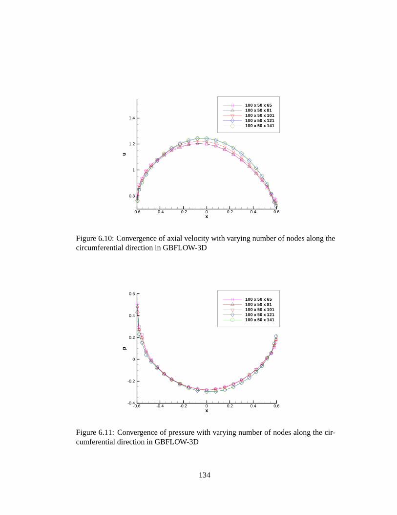
x
u
-0.6 -0.4 -0.2 0 0.2 0.4 0.6
0.8
1
1.2
1.4
100 x 50 x 65100 x 50 x 81100 x 50 x 101100 x 50 x 121100 x 50 x 141
Figure 6.10: Convergence of axial velocity with varying number of nodes along thecircumferential direction in GBFLOW-3D
x
p
-0.6 -0.4 -0.2 0 0.2 0.4 0.6-0.4
-0.2
0
0.2
0.4
0.6100 x 50 x 65100 x 50 x 81100 x 50 x 101100 x 50 x 121100 x 50 x 141
Figure 6.11: Convergence of pressure with varying number of nodes along the cir-cumferential direction in GBFLOW-3D
134
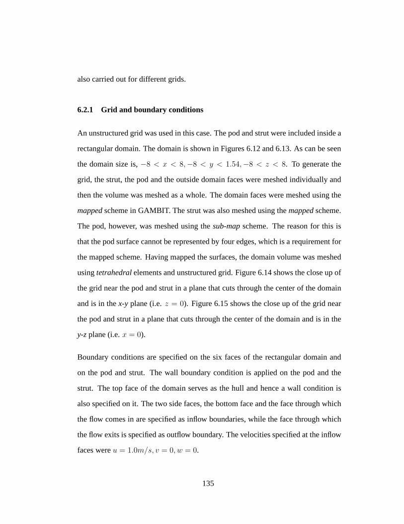
also carried out for different grids.
6.2.1 Grid and boundary conditions
An unstructured grid was used in this case. The pod and strut were included inside a
rectangular domain. The domain is shown in Figures 6.12 and 6.13. As can be seen
the domain size is, −8 < x < 8,−8 < y < 1.54,−8 < z < 8. To generate the
grid, the strut, the pod and the outside domain faces were meshed individually and
then the volume was meshed as a whole. The domain faces were meshed using the
mapped scheme in GAMBIT. The strut was also meshed using the mapped scheme.
The pod, however, was meshed using the sub-map scheme. The reason for this is
that the pod surface cannot be represented by four edges, which is a requirement for
the mapped scheme. Having mapped the surfaces, the domain volume was meshed
using tetrahedral elements and unstructured grid. Figure 6.14 shows the close up of
the grid near the pod and strut in a plane that cuts through the center of the domain
and is in the x-y plane (i.e. z = 0). Figure 6.15 shows the close up of the grid near
the pod and strut in a plane that cuts through the center of the domain and is in the
y-z plane (i.e. x = 0).
Boundary conditions are specified on the six faces of the rectangular domain and
on the pod and strut. The wall boundary condition is applied on the pod and the
strut. The top face of the domain serves as the hull and hence a wall condition is
also specified on it. The two side faces, the bottom face and the face through which
the flow comes in are specified as inflow boundaries, while the face through which
the flow exits is specified as outflow boundary. The velocities specified at the inflow
faces were u = 1.0m/s, v = 0, w = 0.
135
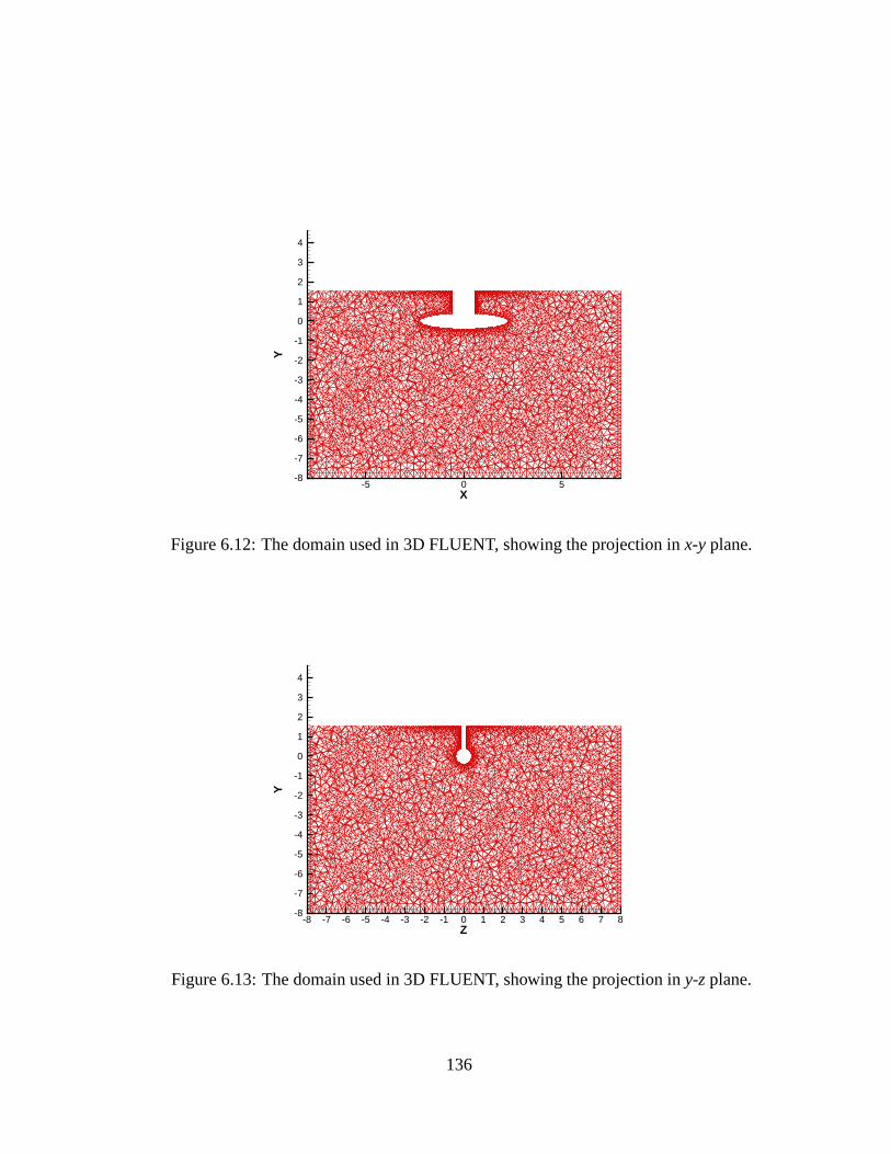
X
Y
-5 0 5-8
-7
-6
-5
-4
-3
-2
-1
0
1
2
3
4
Figure 6.12: The domain used in 3D FLUENT, showing the projection in x-y plane.
Z
Y
-8 -7 -6 -5 -4 -3 -2 -1 0 1 2 3 4 5 6 7 8-8
-7
-6
-5
-4
-3
-2
-1
0
1
2
3
4
Figure 6.13: The domain used in 3D FLUENT, showing the projection in y-z plane.
136

X
Y
-2 -1 0
-0.5
0
0.5
1
1.5
Figure 6.14: Close up of the grid used in 3D FLUENT near the pod and strut in thex-y plane.
Z
Y
-1 -0.5 0 0.5 1
-0.4
-0.2
0
0.2
0.4
0.6
0.8
1
Figure 6.15: Close up of the grid used in 3D FLUENT near the pod and strut in they-z plane.
137

X
Ux
-0.5 0 0.5
0.7
0.8
0.9
1
1.1
1.2
1.3
1.4
1.5 65 nodes on pod
90 nodes on pod
105 nodes on pod
Figure 6.16: Convergence of axial velocity with varying number of nodes on the podusing FLUENT-3D (inviscid).
6.2.2 Inviscid Results
Convergence studies were carried out by varying the number of nodes on the pod.
Since the grid is unstructured, by increasing the number of nodes on the pod, the
cells near the pod and strut get finer. Comparison of pressures and velocities is
carried out at the same location as shown in Figure 6.4. Figures 6.16 and 6.17 show
the convergence of axial velocity and pressure with different grid sizes, respectively.
6.2.3 Viscous Results
Viscous runs were carried out using the same unstructured grids detailed above.
The run parameters for the viscous runs are shown in Table 6.1. Since the grids
are unstructured and no boundary layer is present on the wall, the y+ is very high.
138

X
Cp
-0.5 -0.25 0 0.25 0.5-0.4
-0.3
-0.2
-0.1
0
0.1
0.2
0.3
0.4
65 nodes on pod
90 nodes on pod
105 nodes on pod
Figure 6.17: Convergence of pressure with varying number of nodes on the podusing FLUENT-3D (inviscid).
Solver 3DDP
Model k − ε
Density 998.2
Viscosity 1 × 10⁻³
Cµ 0.09
Reynolds Number 4.52 × 10⁶
Inflow velocity 1.0
k 0.0009227
ε 2.193 × 10⁻⁵
Table 6.1: Run parameters for 3-D viscous FLUENT
139

X
Y+
-2 -1 0 1 2
100
200
300
400
500
600
Figure 6.18: y+ distribution over the 3D pod and strut.
Figure 6.18 shows the y+ distribution along the pod and the strut. As can be seen
the y+ is almost 700, with the higher values taking place over the surface of the pod.
Hence, the solution might not be trustworthy. To judge the accuracy of the solution
a test with the axisymmetric case was carried out. As shown in Figure 4.22 the y+
for the axisymmetric viscous case was about 40. The grid for the axisymmetric case
was modified and made coarser such that the resultant y+ was around 700. The
solution, namely, the pressure distribution along the body and the wall shear stress
from both cases were compared to each other. It was observed that the distribution
was not very different and hence it was deduced that the solution with a y+ of 700
is acceptable. The convergence of the velocities and pressures is shown in Figures
6.20 and 6.21. The velocities and pressures are compared at a location just after the
strut, x = 1.01 and in z = 0 plane. The location is shown in Figure 6.19. The
different grids used are unstructured and hence the number of nodes specified refer
to the number of nodes on the pod edge before it is meshed.
140

X
Y
Z
x=1.01, z=0
x=1.0, y=1.0
Figure 6.19: Locations behind the strut where the velocity and pressure comparisonsare carried out for viscous 3D FLUENT.
Ux
Y
0.5 1
0.4
0.5
0.6
0.7
0.8
0.9
1
1.1
1.2
1.3
1.4
1.570 nodes on pod
90 nodes on pod
105 nodes on pod
Figure 6.20: Convergence of axial velocity with varying number of nodes on the podusing FLUENT-3D (viscous), Re = 4.52 × 10⁶.
141

Cp
Y
-0.5 0 0.5
0.4
0.5
0.6
0.7
0.8
0.9
1
1.1
1.2
1.3
1.4
1.570 nodes on pod
90 nodes on pod
105 nodes on pod
Figure 6.21: Convergence of pressure with varying number of nodes on the podusing FLUENT-3D (viscous), Re = 4.52 × 10⁶.
6.3 Comparison among different methods
A comparison of velocities and pressures predicted by GBFLOW-3D, inviscid
FLUENT-3D and BEM is carried out. The details of the boundary element method
as well as convergence studies are detailed in [Gupta 2004]. In this section the results
of Gupta are used in the comparison. The GBFLOW-3D solution used is from the
grid with cells clustered near the strut and k = 121. Figures 6.22 and 6.23 show the
comparison of the axial velocity and the pressure at the location as shown in Figure
6.4. As it can be seen, the results from FLUENT and BEM agree very well with each
other and that the axial velocity obtained from GBFLOW-3D is somewhat larger at
the leading edge and smaller at the mid part of the strut. However, the pressures
predicted from the three methods seem to be in closer agreement with each other.
Comparisons are also carried out between inviscid and viscous FLUENT at the
locations shown in Figure 6.19. Figures 6.24 and 6.25 show the comparison for the
142

X
U_x
-0.5 0 0.50
0.2
0.4
0.6
0.8
1
1.2
1.4
FLUENT (inviscid)
GBFLOW-3D
BEM
Figure 6.22: Comparison of axial velocity on the pod among the different methods.
X
C_p
-0.5 0 0.5-0.5
-0.4
-0.3
-0.2
-0.1
0
0.1
0.2
0.3
0.4
0.5
FLUENT (inviscid)
GBFLOW-3D
BEM
Figure 6.23: Comparison of pressure on the pod among the different methods.
143

Ux
Y
0.5 1
0.4
0.5
0.6
0.7
0.8
0.9
1
1.1
1.2
1.3
1.4
1.5
FLUENT (inviscid)
FLUENT (viscous)
Figure 6.24: Comparison of axial velocity among inviscid and viscous 3D FLUENTat the line on the x-z plane, Re = 4.52 × 10⁶.
line on the x-z plane and Figures 6.26 and 6.27 shows the comparison at the line on
the x-y plane. It can be seen that the velocity in the case of the viscous flow is lower,
since the presence of the strut (wall) causes shear and decreases the velocity.
144

Cp
Y
-0.5 -0.4 -0.3 -0.2 -0.1 0 0.1 0.2 0.3 0.4 0.5
0.4
0.5
0.6
0.7
0.8
0.9
1
1.1
1.2
1.3
1.4
1.5
FLUENT (inviscid)
FLUENT (viscous)
Figure 6.25: Comparison of pressure among inviscid and viscous 3D FLUENT atthe line on the x-z plane, Re = 4.52 × 10⁶.
Z
U
-1 -0.5 0 0.5 1
0.86
0.88
0.9
0.92
0.94
0.96
0.98
1
1.02
1.04
1.06
1.08
1.1
FLUENT (inviscid)FLUENT (viscous)
Figure 6.26: Comparison of axial velocity among inviscid and viscous 3D FLUENTat the line on the x-y plane, Re = 4.52 × 10⁶.
145

Z
Cp
-1 -0.5 0 0.5 1
-0.04
-0.02
0
0.02
0.04
0.06
0.08
0.1
FLUENT (inviscid)FLUENT (viscous)
Figure 6.27: Comparison of pressure among inviscid and viscous 3D FLUENT atthe line on the x-y plane, Re = 4.52 × 10⁶.
146

Chapter 7
Conclusions and Recommendations
7.1 Conclusions
As mentioned in earlier chapters, podded propulsion systems are now being widely
used on commercial or naval vessels. Hence, the prediction of the performance of
such systems is of utmost importance. [Kakar 2002] outlines some preliminary work
carried out towards the numerical prediction of performance of podded propellers.
This work was furthered in [Gupta 2004], where a 3-dimensional Euler solver was
used to predict the flow around podded propulsors. The Euler solver was also ex-
tended to solve for yaw angles of attack. In this thesis, the Vortex Lattice Method
has been coupled with an axi-symmetric Euler solver and an axi-symmetric viscous
flow solver, to predict the performance of podded propellers and also estimate the
effects of viscosity on the predictions.
The axi-symmetric Euler solver was validated by carrying out comparisons with a
BEM solver and inviscid FLUENT. Viscous runs were also carried out using the
viscous flow solver in FLUENT and the frictional force on the body was estimated.
This was compared to the force obtained from the empirical ITTC formula which
is used by the inviscid solver (GBFLOW) to account for the frictional force. It was
found that the ITTC formula provided a reasonable approximation for the frictional
147
force acting on the pod.
The pod with a propeller case was solved via coupling between MPUF3A and
GBFLOW or FLUENT. Both inviscid and viscous flow solvers were used in FLU-
ENT. It was seen that viscosity did not affect the performance of the pull type podded
unit significantly but the performance of the push type and the twin type (especially
the aft propeller) podded unit changed significantly. Nevertheless, in the case of a
twin propeller pod, the total force acting on the pod was not found to be influenced
appreciably by the effects of viscosity. The k − ε viscous model in FLUENT was
found to be over dissipative and hence the RSM model was used. The 3-dimensional
problem (pod with strut) was also solved without the propeller and comparisons
were carried out with FLUENT and BEM. An alternate grid arrangement was used
in GBFLOW-3D which seemed to provide more accurate results.
As detailed in Chapter 3, coupling between the VLM and the BEM was carried
out. However, the method is not in complete working condition yet. More details
regarding the method and tests carried out are included in the term report submitted
for the class, “Hydrodynamics of Propulsors and Dynamic Positioning System”.
7.2 Recommendations
This thesis is a first step in predicting the effects of viscosity via coupling of MPUF3A
with FLUENT. Some recommendations for improvement and furthering this work
are listed below:
• The coupling between 3D FLUENT and MPUF3A should be completed to
solve the pod, strut and propeller problem iteratively. The solution to the
148

problem using the 3D body forces in FLUENT (via source terms) requires
prohibitively large run times and efforts should be made to reduce it. This
happens because the source terms are incorporated in FLUENT via UDF, and
they have to be evaluated at every iteration. A change in the FLUENT source
code maybe required to overcome this problem. Once this is done, the effects
of viscosity can be estimated in the 3-dimensional case.
• A better grid for GBFLOW-3D should be developed to provide more accurate
flow field results, especially near the strut region.
• The coupling between BEM and MPUF3A should be completed in order to
assess the accuracy of the image model used in MPUF-3A when coupled with
GBFLOW. Although individual modules of the coupling seem to work well,
the overall solution does not. The reason for this has to be investigated.
• More validation with measurements are needed, especially in the case of push
type podded propellers. In particular the flow field just upstream of the pro-
peller should be measured and compared with our predictions.
149

Appendix A
150

Pod geometry used for 3-X and 3-D runs
X R X R
-2.265 0.0E+0 -0.0853889 0.40468
-2.0800001 0.16028973 0.2492491 0.4024901
-1.8950001 0.22174709 0.39291653 0.39880943
-1.71 0.26552885 0.50475215 0.3947888
-1.5250001 0.29938104 0.5756959 0.391669
-1.34 0.32648843 0.6 0.3904801
-1.155 0.34837907 0.785 0.37985682
-0.97 0.36596354 0.97 0.36596357
-0.78499996 0.37985682 1.1550001 0.34837904
-0.6 0.3904801 1.3400002 0.3264884
-0.57569575 0.39166897 1.5250001 0.29938104
-0.50475215 0.39478877 1.7100002 0.26552876
-0.39291644 0.39880946 1.8950001 0.22174709
-0.24924898 0.40249016 2.0800001 0.16029005
2.265 0.0E+0
Table 1: The pod geometry used by [Szantyr 2001a]
151
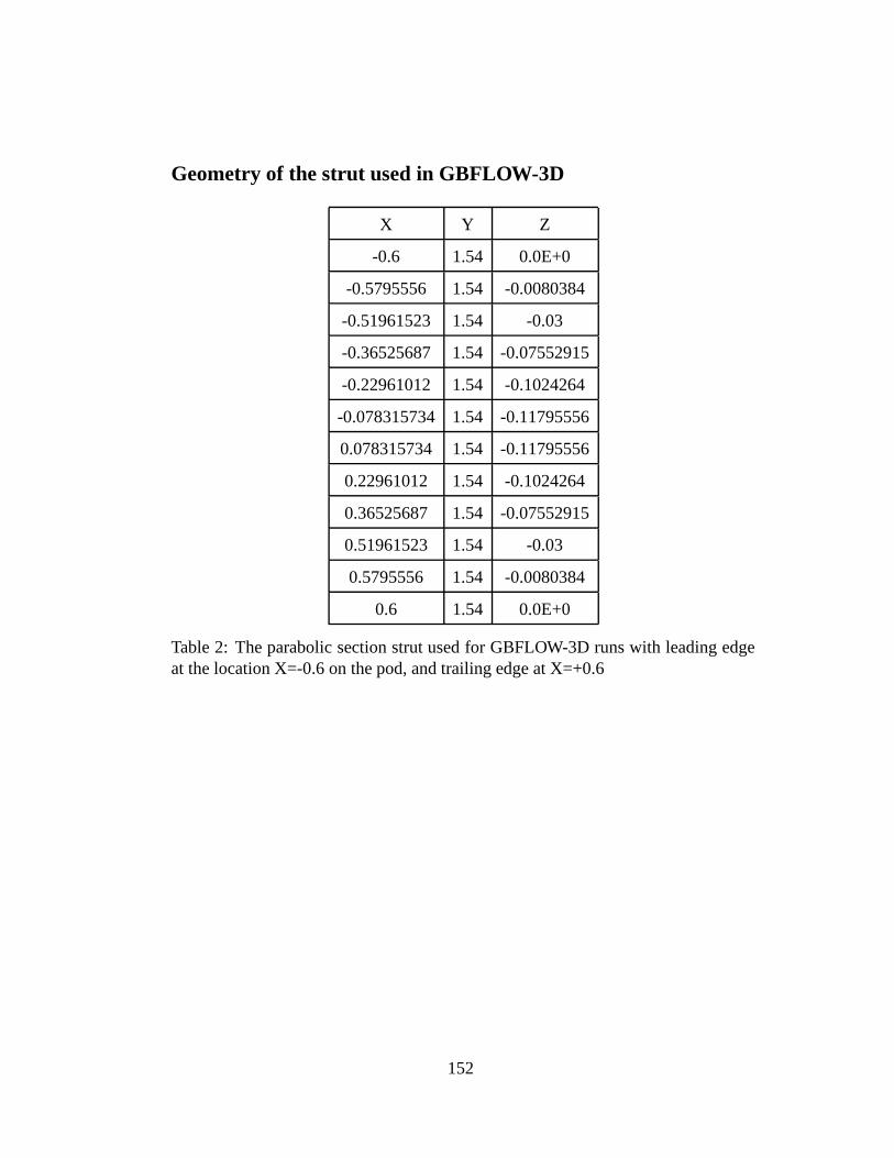
Geometry of the strut used in GBFLOW-3D
X Y Z
-0.6 1.54 0.0E+0
-0.5795556 1.54 -0.0080384
-0.51961523 1.54 -0.03
-0.36525687 1.54 -0.07552915
-0.22961012 1.54 -0.1024264
-0.078315734 1.54 -0.11795556
0.078315734 1.54 -0.11795556
0.22961012 1.54 -0.1024264
0.36525687 1.54 -0.07552915
0.51961523 1.54 -0.03
0.5795556 1.54 -0.0080384
0.6 1.54 0.0E+0
Table 2: The parabolic section strut used for GBFLOW-3D runs with leading edgeat the location X=-0.6 on the pod, and trailing edge at X=+0.6
152

Geometry of the strut used by [Szantyr 2001a]
X Y Z
-0.6 1.54 0.0E+0
-0.5756959 1.54 -0.068673864
-0.50475215 1.54 -0.13486163
-0.39291653 1.54 -0.19476245
-0.2492491 1.54 -0.23895688
-0.08538896 1.54 -0.2590484
0.0853889 1.54 -0.2476123
0.24924898 1.54 -0.20349935
0.39291644 1.54 -0.13812754
0.50475215 1.54 -0.070037215
0.57569575 1.54 -0.018887708
0.6 1.54 0.0E+0
Table 3: The strut used by [Szantyr 2001a] for the experimental measurements. Itis a NACA066 section, and has the leading edge at the location X=-0.6 on the pod,and trailing edge at X=+0.6
153

Front Propeller Geometry used in [Szantyr 2001a]
r/R P/D Rk/D Skew C/D F/C T/D
0.3027 0.8 0.00 0.00 0.3252 0.0621 0.0404
0.3463 0.8 0.00 0.00 0.3794 0.0506 0.0384
0.4552 0.8 0.00 0.00 0.5148 0.0314 0.0323
0.5642 0.8 0.00 0.00 0.6291 0.0207 0.0261
0.6731 0.8 0.00 0.00 0.7179 0.0139 0.0200
0.7821 0.8 0.00 0.00 0.7616 0.0090 0.0138
0.8910 0.8 0.00 0.00 0.7165 0.0053 0.0076
0.9455 0.8 0.00 0.00 0.5938 0.0038 0.0045
1.000 0.8 0.00 0.00 0.2000 0.0000 0.0000
Table 4: Front propeller geometry. The front propeller placed at the location -1.1899on the pod
154
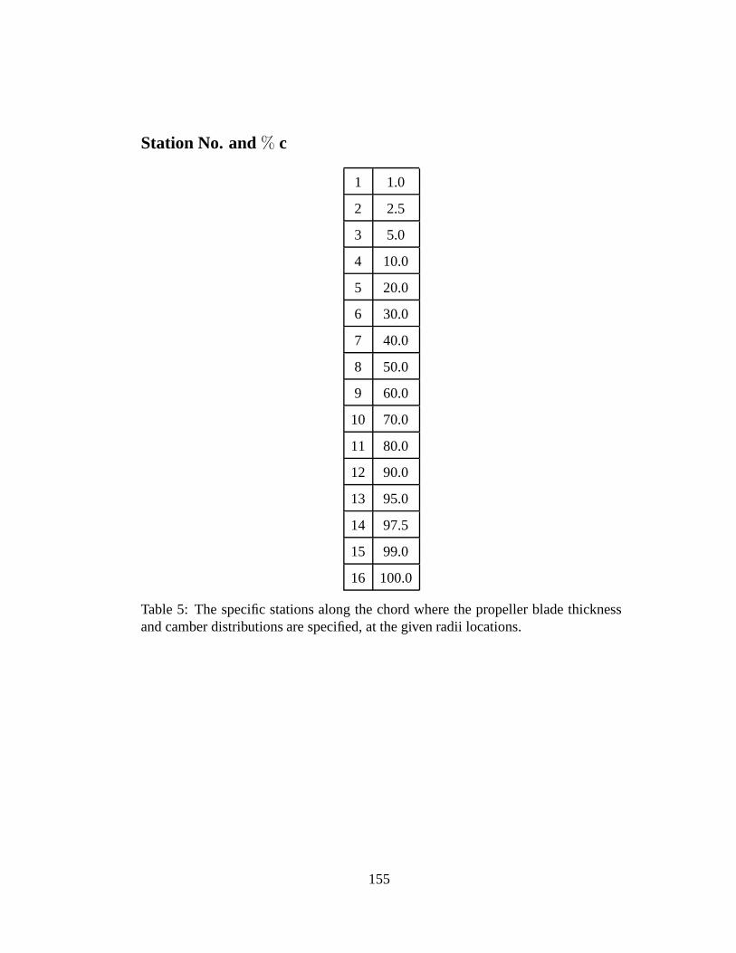
Station No. and % c
1 1.0
2 2.5
3 5.0
4 10.0
5 20.0
6 30.0
7 40.0
8 50.0
9 60.0
10 70.0
11 80.0
12 90.0
13 95.0
14 97.5
15 99.0
16 100.0
Table 5: The specific stations along the chord where the propeller blade thicknessand camber distributions are specified, at the given radii locations.
155

Camber Distribution, f/C
Radii 0.3027 0.3463 0.4552 0.5642 0.6731 0.7821 0.8910 0.9455 1.000
station1 0.0041 0.0029 0.0014 0.0009 0.0006 0.0005 0.0003 0.0003 0.0000
station2 0.0099 0.0071 0.0034 0.0023 0.0016 0.0011 0.0007 0.0007 0.0000
station3 0.0183 0.0132 0.0065 0.0044 0.0030 0.0021 0.0014 0.0012 0.0000
station4 0.0314 0.0232 0.0120 0.0080 0.0055 0.0037 0.0024 0.0020 0.0000
station5 0.0466 0.0362 0.0206 0.0137 0.0093 0.0061 0.0038 0.0029 0.0000
station6 0.0547 0.0439 0.0265 0.0176 0.0118 0.0077 0.0046 0.0034 0.0000
station7 0.0605 0.0491 0.0301 0.0199 0.0134 0.0087 0.0051 0.0037 0.0000
station8 0.0621 0.0506 0.0314 0.0207 0.0139 0.0090 0.0053 0.0038 0.0000
station9 0.0605 0.0491 0.0301 0.0199 0.0134 0.0087 0.0051 0.0037 0.0000
station10 0.0547 0.0439 0.0265 0.0176 0.0118 0.0077 0.0046 0.0034 0.0000
station11 0.0466 0.0362 0.0206 0.0137 0.0093 0.0061 0.0038 0.0029 0.0000
station12 0.0313 0.0232 0.0120 0.0080 0.0055 0.0037 0.0024 0.0020 0.0000
station13 0.0180 0.0131 0.0065 0.0044 0.0030 0.0021 0.0014 0.0012 0.0000
station14 0.0096 0.0069 0.0033 0.0023 0.0016 0.0011 0.0007 0.0006 0.0000
station15 0.0040 0.0028 0.0014 0.0009 0.0006 0.0005 0.0003 0.0003 0.0000
Table 6: The camber distribution specified at the nine radii locations specified in thegeometry file and at specific stations along the chord.
156
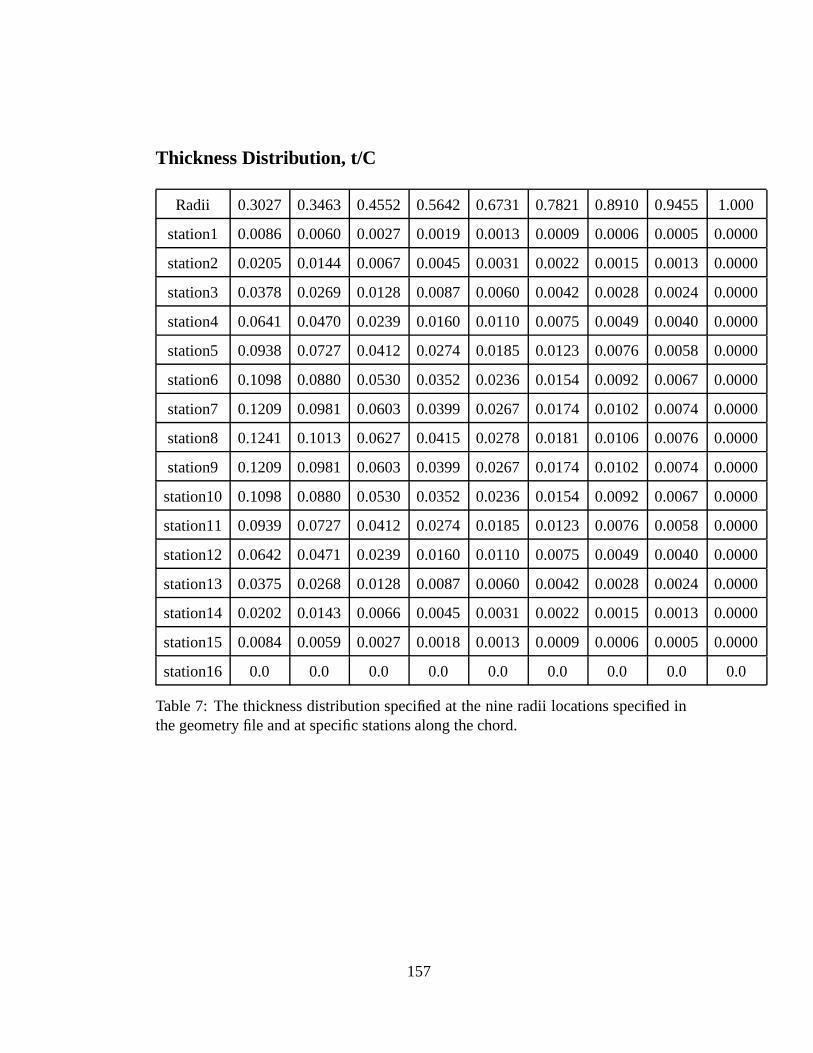
Thickness Distribution, t/C
Radii 0.3027 0.3463 0.4552 0.5642 0.6731 0.7821 0.8910 0.9455 1.000
station1 0.0086 0.0060 0.0027 0.0019 0.0013 0.0009 0.0006 0.0005 0.0000
station2 0.0205 0.0144 0.0067 0.0045 0.0031 0.0022 0.0015 0.0013 0.0000
station3 0.0378 0.0269 0.0128 0.0087 0.0060 0.0042 0.0028 0.0024 0.0000
station4 0.0641 0.0470 0.0239 0.0160 0.0110 0.0075 0.0049 0.0040 0.0000
station5 0.0938 0.0727 0.0412 0.0274 0.0185 0.0123 0.0076 0.0058 0.0000
station6 0.1098 0.0880 0.0530 0.0352 0.0236 0.0154 0.0092 0.0067 0.0000
station7 0.1209 0.0981 0.0603 0.0399 0.0267 0.0174 0.0102 0.0074 0.0000
station8 0.1241 0.1013 0.0627 0.0415 0.0278 0.0181 0.0106 0.0076 0.0000
station9 0.1209 0.0981 0.0603 0.0399 0.0267 0.0174 0.0102 0.0074 0.0000
station10 0.1098 0.0880 0.0530 0.0352 0.0236 0.0154 0.0092 0.0067 0.0000
station11 0.0939 0.0727 0.0412 0.0274 0.0185 0.0123 0.0076 0.0058 0.0000
station12 0.0642 0.0471 0.0239 0.0160 0.0110 0.0075 0.0049 0.0040 0.0000
station13 0.0375 0.0268 0.0128 0.0087 0.0060 0.0042 0.0028 0.0024 0.0000
station14 0.0202 0.0143 0.0066 0.0045 0.0031 0.0022 0.0015 0.0013 0.0000
station15 0.0084 0.0059 0.0027 0.0018 0.0013 0.0009 0.0006 0.0005 0.0000
station16 0.0 0.0 0.0 0.0 0.0 0.0 0.0 0.0 0.0
Table 7: The thickness distribution specified at the nine radii locations specified inthe geometry file and at specific stations along the chord.
157
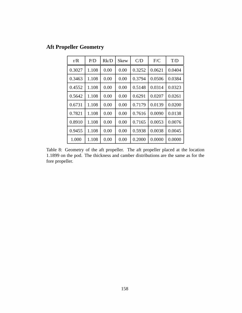
Aft Propeller Geometry
r/R P/D Rk/D Skew C/D F/C T/D
0.3027 1.108 0.00 0.00 0.3252 0.0621 0.0404
0.3463 1.108 0.00 0.00 0.3794 0.0506 0.0384
0.4552 1.108 0.00 0.00 0.5148 0.0314 0.0323
0.5642 1.108 0.00 0.00 0.6291 0.0207 0.0261
0.6731 1.108 0.00 0.00 0.7179 0.0139 0.0200
0.7821 1.108 0.00 0.00 0.7616 0.0090 0.0138
0.8910 1.108 0.00 0.00 0.7165 0.0053 0.0076
0.9455 1.108 0.00 0.00 0.5938 0.0038 0.0045
1.000 1.108 0.00 0.00 0.2000 0.0000 0.0000
Table 8: Geometry of the aft propeller. The aft propeller placed at the location1.1899 on the pod. The thickness and camber distributions are the same as for thefore propeller.
158

Bibliography
Achkinadze, A., Berg, A., Krasilnikov, V. and Stepanov, I. [2003], ‘Numerical anal-
ysis of podded and steering systems using a velocity based source boundary ele-
ment method with modified trailing edge’.
Blenkey, N. [1997], ‘Getting twin propeller efficiency from a pod’, Marine Log .
Breslin, J., Van Houten, R., Kerwin, J. and Johnsson, C.-A. [1982], ‘Theoretical
and experimental propeller-induced hull pressures arising from intermittent blade
cavitation, loading, and thickness’, Trans. SNAME 90.
Chicherin, I., A., Lobatchev, M., Pustoshny, A., V. and Sanchez-Caja, A. [2004],
‘On a propulsion prediction procedure for ships with podded propulsors using
rans-code analysis’, Proceedings of the First International COnference on Tech-
nological Advances in Podded Propulsion pp. pp. 223–236.
Choi, J.-K. [2000], Vortical Inflow – Propeller Interaction Using an Unsteady Three-
Dimensional Euler Solver, PhD thesis, Department of Civil Engineering, The Uni-
versity of Texas at Austin.
Choi, J.-K. and Kinnas, S. [1998], A 3-D Euler solver and its application on the
analysis of cavitating propellers, in ‘Proceedings of the 25th ATTC’, American
Towing Tank Conference, Iowa City, Iowa.
159

Choi, J.-K. and Kinnas, S. [2000a], Non-axisymmetric effective wake prediction
by using an unsteady three-dimensional Euler solver, in ‘Propellers/Shafting ’00
Symposium’, Soc. Naval Arch. & Marine Engnrs., Virginia Beach, VA.
Choi, J.-K. and Kinnas, S. [2000b], An unsteady 3-D Euler solver coupled with
a cavitating propeller analysis method, in ‘23rd Symposium on Naval Hydrody-
namics’, Val de Reuil, France.
Choi, J.-K. and Kinnas, S. [2001], ‘Prediction of Non-axisymmetric Effective Wake
by a Three-Dimensional Euler Solver’, Journal of Ship Research 45(1), pp. 13–33.
Choi, J.-K. and Kinnas, S. [2003], ‘Prediction of unsteady effective wake by an euler
solver/vortex-lattice coupled method’, Journal of Ship Research, Vol. 47, pp.131-
144 .
Choi, J. and Kinnas, S. [2000c], An unsteady three-dimensional euler solver coupled
with a cavitating propeller analysis method, in ‘The 23rd Symposium on Naval
Hydrodynamics’, Val de Reuil, France.
Chorin, A. J. [1967], ‘A numerical method for solving incompressible viscous flow
problems’, Journal of Computational Physics 2, pp.12–26.
Dai, C., Gorski, J. and Haussling, H. [1991], Computation of an integrated ducted
propulsor/stern performance in axisymmetric flow, in ‘Propellers/Shafting ’91
Symposium’, Soc. Naval Arch. & Marine Engnrs., Virginia Beach, VA.
FLUENT [2003], Fluent 6.1 user’s guide, User’s manual, FLUENT.
Gawn, R. and Burrill, L. [1957], ‘Effect of cavitation on the performance of a series
of 16 in. model propellers’, Transactions INA 99, pp. 690–728.
160

Ghassemi, H. and Allievi, A. [1999], ‘A Computational Method for the Analysis of
Fluid Flow and Hydrodynamic Performance of Conventional and Podded Propul-
sion Systems’, Oceanic Engineering International 3(1), pp. 101–115.
Greeley, D. and Kerwin, J. [1982], ‘Numerical methods for propeller design and
analysis in steady flow’, Trans. SNAME vol 90.
Griffin, P. [1998], Computational techniques for the design and analysis of cavitating
propeller blades, Master’s thesis, UT Austin, Dept. of Civil Engineering.
Gu, H. and Kinnas, S. A. [2003], Modeling of contra-rotating and ducted pro-
pellers via coupling of a vortex-lattice with a finite volume method, in ‘Pro-
pellers/Shafting 2003’.
Gu, H., Natarajan, S., Gupta, A. and Kinnas, S. [2003], GBFLOW (version 1.1)
user’s manual, Ocean Engineering Report 03-3, Ocean Engineering Group, UT
Austin, Austin, TX.
Gupta, A. [2004], Numerical prediction of flows around podded propulsors, Master’s
thesis, Department of Civil Engineering, The University of Texas at Austin.
Hsin, C.-Y., Chou, S.-K. and Chen, W.-C. [2002], A new propeller design method
for the pod propulsion system, in ‘Proceedings of Twenty-Fourth Symposium on
Naval Hydrodynamics’, Fukuoka, Japan.
Huang, T. and Cox, B. [1977], Interaction of afterbody boundary layer and pro-
peller, in ‘Symposium on Hydrodynamics of Ship and Offshore Propulsion Sys-
tem’, Høvik outside Oslo.
161

Huang, T. and Groves, N. [1980], Effective wake : Theory and experiment, in ‘13th
Symposium on Naval Hydrodynamics’, Tokyo.
Huang, T., Wang, H., Santelli, N. and Groves, N. [1976], Propeller/stern bound-
ary layer interaction on axisymmetric bodies : Theory and experiment, Technical
Report DTNSRDC 76-0113, DTNSRDC.
Hughes, M. [1993], Analysis of Multi-component Ducted Propulsors in Unsteady
Flow, PhD thesis, M.I.T., Department of Ocean Engineering.
Hughes, M. and Kinnas, S. [1991], A analysis method for a ducted propeller with
pre-swirl stator blades, in ‘Propellers/Shafting ’91 Symposium’, Soc. Naval Arch.
& Marine Engnrs., Virginia Beach, VA, pp. 1–8 (paper No. 15).
Hughes, M. and Kinnas, S. [1993], Unsteady flows around multi-component inte-
grated propulsors, in ‘Forum on Unsteady Flows, (FED-Vol. 157)’, Fluids Engi-
neering Division, ASME, pp. 21–31.
HYDROCOMP, I. [1999], Modeling tractor-style azimuthing podded drives, Tech-
nical Report 127, HYDROCOMP Inc.
Islam, M., Taylor, R., Quinton, J., Veitch, B. and Bose, N. [2004], ‘Numerical inves-
tigation on hydrodynamic performance of podded propeller’, Proceedings of the
First International COnference on Technological Advances in Podded Propulsion
pp. 513–526.
Kakar, K. [2002], Computational Modeling of FPSO Hull Roll Motions and Two-
component Marine Propulsion Systems, Master’s thesis, Department of Civil En-
gineering, The University of Texas at Austin.
162

Kerwin, J. E., Coney, W. B. and Hsin, C.-Y. [1988], Hydrodynamic aspects of pro-
peller/stator design, in ‘Proceedings of the Propellers ’88 Symposium’, number 3,
SNAME, Virginia Beach, VA.
Kerwin, J., Keenan, D., Black, S. and Diggs, J. [1994], ‘A coupled viscous/potential
flow design method for wake adapted multi-stage, ducted propulsors using gener-
alized geometry’, Trans. SNAME 102.
Kerwin, J., Kinnas, S., Lee, J. and Shih, W. Z. [1987], in ‘A surface panel method
for the hydrodynamic analysis of ducted propellers’, Vol. 95.
Kerwin, J., Kinnas, S., Wilson, M. and McHugh, J. [1986], Experimental and analyt-
ical techniques for the study of unsteady propeller sheet cavitation, in ‘Proceed-
ings of the Sixteenth Symposium on Naval Hydrodynamics’, Berkeley, California,
pp. 387–414.
Kerwin, J. and Lee, C.-S. [1978], ‘Prediction of steady and unsteady marine pro-
peller performance by numerical lifting-surface theory’, Trans. SNAME vol 86.
Kerwin, J., Taylor, T., Black, S. and McHugh, G. [1997a], A coupled lifting-surface
analysis technique for marine propulsors in steady flow, in ‘Propellers/Shafting
’97 Symposium’, Soc. Naval Arch. & Marine Engnrs., Virginia Beach, VA, pp. 1–
15 (Paper No. 20).
Kerwin, J., Taylor, T., Black, S. and McHugh, G. [1997b], ‘A coupled lifting-surface
analysis technique or marine propellers in steady flow’, Proceedings of the Pro-
pellers/Shafting Symposium pp. pp. 20/1–15.
Kinnas, S. [1991], ‘Leading-edge corrections to the linear theory of partially cavi-
tating hydrofoils’, Journal of Ship Research 35(1), pp. 15–27.
163

Kinnas, S. [1992], ‘A general theory for the coupling between thickness and loading
for wings and propellers’, Journal of Ship Research 36(1), pp. 59–68.
Kinnas, S., Choi, J., Lee, H. and Young, J. [2000], Numerical cavitation tunnel,
in ‘NCT50, International Conference on Propeller Cavitation’, Newcastle upon
Tyne, England.
Kinnas, S., Choi, J., Lee, H., Young, Y., Gu, H., Kakar, K. and Natarajan, S. [2002],
‘Prediction of cavitation performance of single/multi-component propulsors and
their interaction with the hull’, Trans. SNAME .
Kinnas, S. and Fine, N. [1989], Theoretical prediction of the midchord and face un-
steady propeller sheet cavitation, in ‘Proceedings of the Fifth International Con-
ference on Numerical Ship Hydrodynamics’, Hiroshima, Japan.
Kinnas, S., Griffin, P., Choi, J.-K. and Kosal, E. [1998a], ‘Automated design of
propulsor blades for high-speed ocean vehicle applications’, Trans. SNAME 106.
Kinnas, S., Griffin, P., Choi, J.-K. and Kosal, E. [1998b], ‘Automated design of
propulsor blades for high-speed ocean vehicle applications’, Trans. SNAME 106.
Kinnas, S., Gu, H., Gupta, A. and Lee, H. [2004], Numerical prediction of the per-
formance of podded propulsors and ducted propellers, in ‘Proceedings of the 13th
Offshore Symposium on The Application of Emerging Technologies’, Houston,
Texas, pp. 19–34.
Kinnas, S., Lee, H., Gu, H. and Gupta, A. [2004], Prediction of performance of
ducted and podded propellers, in ‘25th Symposium on Naval Hydrodynamics’,
St. John’s, Newfoundland and Labrador, Canada.
164
Kinnas, S., Lee, H., Gu, H., Yu, Y., Sun, H., Vinayan, V., Kacham, B., Mishra,
B. and Deng, Y. [2004], ‘University/navy/industry consortium on cavitation per-
formance of high speed propulsors - presentations and progress reports - 22nd
steering committee meeting’.
Kinnas, S. and Pyo, S. [1999], ‘Cavitating propeller analysis including the effects of
wake alignment’, Journal of Ship Research 43(1), pp. 38–47.
Kosal, E. [1999], Improvements and enhancements in the numerical analysis and
design of cavitating propeller blades, Master’s thesis, UT Austin, Dept. of Civil
Engineering.
Kudo, T. and Kinnas, S. [1995], Application of vortex/source lattice method on su-
percavitating propellers, in ‘24th American Towing Tank Conference’, College
Station, TX.
Lee, C.-S. [1979], Prediction of Steady and Unsteady Performance of Marine Pro-
pellers with or without Cavitation by Numerical Lifting Surface Theory, PhD the-
sis, M.I.T., Department of Ocean Engineering.
Lewis, E. [1988], Principles of Naval Architecture, Society of Naval Architects and
Marine Engineers.
Maskew, B. [1990], USAERO, A Time-stepping Analysis Method for the Flow
About Multiple Bodies in General Motions, User’s Manual , Technical report,
Analytical Methods, Inc., Redmond, WA.
Morino, L. and Kuo, C.-C. [1974], ‘Subsonic Potential Aerodynamic for Complex
Configurations : A General Theory’, AIAA Journal vol 12(no 2), pp 191–197.
165

Natarajan, S. [2003], Computational Modeling of Marine Rudders and Multi-
component Marine Propulsion Systems, Master’s thesis, Department of Civil En-
gineering, The University of Texas at Austin.
Ni, R.-H. [1982], ‘A multiple-grid scheme for solving the Euler equations’, AIAA
Journal 20(11), pp.1565–1571.
Ohashi, K. and Hino, T. [2004], ‘Numerical simulations of the flows around a ship
with podded propulsor’, Proceedings of the First International COnference on
Technological Advances in Podded Propulsion pp. pp. 211–222.
Ohkusu, M., ed. [1996], Advances in Marine Hydrodynamics, Computational Me-
chanics Publications, Southampton, UK.
Sanchez-Caja, A., Rautaheimo, P. and Siikonen, T. [1999], Computation of the in-
compressible viscous flow around a tractor thruster using a sliding-mesh tech-
nique, in ‘Proceedings of Seventh International Conference on Numerical Ship
Hydrodynamics’, France.
Shih, W.-Z. [1988], A Combined Euler Equation/Surface Panel Solution to The
Shear Interaction Problem of An Open or Ducted Propeller, PhD thesis, Depart-
ment of Ocean Engineering, M.I.T.
Stern, F., Kim, H., Patel, V. and Chen, H. [1988a], ‘Computation of viscous flow
around propeller-shaft configurations’, Journal of Ship Research 32(4), pp.263–
284.
Stern, F., Kim, H., Patel, V. and Chen, H. [1988b], ‘A viscous-flow approach to the
computation of propeller- hull interaction’, Journal of Ship Research 32(4), pp.
246–262.
166

Stern, F., Kim, H., Zhang, D., Kerwin, J. and Jessup, S. [1994], ‘Computation of
viscous flow around propeller-body configurations: Series 60 cb =0.6 ship model’,
Journal of Ship Research 38(2), pp. 137–157.
Szantyr, J. [2001a], ‘Hydrodynamic model experiments with pod propulsors’,
Oceanic Engineering International 5(2), pp. 95–103.
Szantyr, J. [2001b], ‘Hydrodynamic model experiments with pod propulsors’,
Ocean Engineering International 5-2, pp. 95–103.
Tsakonas, S., Jacobs, W. and Liao, P. [1983], ‘Prediction of steady and unsteady
loads and hydrodynamic forces on counterrotating propellers’, Journal of Ship
Research 27(3), pp. 197–214.
Vartdal, L. and Bloch, F. [2001], Ferrycat 120 propulsion aspects and manoeuvring
capabilities, in ‘Proceedings of First International Conference on Double-ended
Ferries’, Molde, Norway.
Vartdal, L., Gjerde, K. M., Bloch, F. and Sittanggang, P. [1999], Application of var-
ious cfd methods in the development of the azipull podded propulsion system,
in ‘The International CFD Conference in Ship Hydrodynamics’, Ulsteinvik, Nor-
way.
Warren, C., Taylor, T. and Kerwin, J. [2000], A coupled viscous/potential-flow
method for the prediction of propulsor-induced maneuvering forces, in ‘Pro-
pellers/Shafting ’00 Symposium’, Soc. Naval Arch. & Marine Engnrs., Virginia
Beach, VA.
167

Yang, C.-J., Wang, G., Tamashima, M., Yamazaki, R. and Koizuka, H. [1992], ‘Pre-
diction of the unsteady performance of contra-rotating propellers by lifting surface
theory’, Trans. of the West-Japan Society of Naval Architects (No. 83), pp. 47–65.
168

Vita
Bikash Mishra was born in Balasore, India on September 22, 1981. He is the
son of Basanta Kumar Mishra and Pushpamitra Mishra. He obtained his Bachelor of
Technology in Naval Architecture and Ocean Engineering from the Indian Institute
of Technology at Madras in July, 2003. He started his Masters program in civil
engineering at The University of Texas at Austin in September, 2003.
Permanent address: 2907 Rio Grande, Austin Texas
This thesis was typeset with LATEX‡ by the author.
‡LATEX is a document preparation system developed by Leslie Lamport as a special version ofDonald Knuth’s TEX Program.
169