Prediction of plant-level tomato biomass and yield using

Tatsumi et al. Plant Methods (2021) 17:77 https://doi.org/10.1186/s13007-021-00761-2

RESEARCH

Prediction of plant-level tomato biomass and yield using machine learning with unmanned aerial vehicle imageryKenichi Tatsumi1* , Noa Igarashi2 and Xiao Mengxue3

Abstract

Background: The objective of this study is twofold. First, ascertain the important variables that predict tomato yields from plant height (PH) and vegetation index (VI) maps. The maps were derived from images taken by unmanned aer-ial vehicles (UAVs). Second, examine the accuracy of predictions of tomato fresh shoot masses (SM), fruit weights (FW), and the number of fruits (FN) from multiple machine learning algorithms using selected variable sets. To realize our objective, ultra-high-resolution RGB and multispectral images were collected by a UAV on ten days in 2020’s tomato growing season. From these images, 756 total variables, including first- (e.g., average, standard deviation, skewness, range, and maximum) and second-order (e.g., gray-level co-occurrence matrix features and growth rates of PH and VIs) statistics for each plant, were extracted. Several selection algorithms (i.e., Boruta, DALEX, genetic algorithm, least absolute shrinkage and selection operator, and recursive feature elimination) were used to select the variable sets useful for predicting SM, FW, and FN. Random forests, ridge regressions, and support vector machines were used to predict the yield using the top five selected variable sets.

Results: First-order statistics of PH and VIs collected during the early to mid-fruit formation periods, about one month prior to harvest, were important variables for predicting SM. Similar to the case for SM, variables collected approximately one month prior to harvest were important for predicting FW and FN. Furthermore, variables related to PH were unimportant for prediction. Compared with predictions obtained using only first-order statistics, those obtained using the second-order statistics of VIs were more accurate for FW and FN. The prediction accuracy of SM, FW, and FN by models constructed from all variables (rRMSE = 8.8–28.1%) was better than that from first-order statis-tics (rRMSE = 10.0–50.1%).

Conclusions: In addition to basic statistics (e.g., average and standard deviation), we derived second-order statistics of PH and VIs at the plant level using the ultra-high resolution UAV images. Our findings indicated that our variable selection method reduced the number variables needed for tomato yield prediction, improving the efficiency of phe-notypic data collection and assisting with the selection of high-yield lines within breeding programs.

Keywords: Tomato yield prediction, Gray-level co-occurrence matrix, Plant-level, Machine learning, Unmanned aerial vehicle

© The Author(s) 2021. This article is licensed under a Creative Commons Attribution 4.0 International License, which permits use, sharing, adaptation, distribution and reproduction in any medium or format, as long as you give appropriate credit to the original author(s) and the source, provide a link to the Creative Commons licence, and indicate if changes were made. The images or other third party material in this article are included in the article’s Creative Commons licence, unless indicated otherwise in a credit line to the material. If material is not included in the article’s Creative Commons licence and your intended use is not permitted by statutory regulation or exceeds the permitted use, you will need to obtain permission directly from the copyright holder. To view a copy of this licence, visit http:// creat iveco mmons. org/ licen ses/ by/4. 0/. The Creative Commons Public Domain Dedication waiver (http:// creat iveco mmons. org/ publi cdoma in/ zero/1. 0/) applies to the data made available in this article, unless otherwise stated in a credit line to the data.

BackgroundTomato (Solanum lycopersicum L.) is one of the most widely and globally grown vegetables in the world and plays an important role in human health maintenance [1]. In 2018, the annual production of fresh tomatoes was about 180 million tons globally [2]. Approximately a

Open Access

Plant Methods

*Correspondence: [email protected] Department of Environmental and Agricultural Engineering, Tokyo University of Agriculture and Technology, 3-5-8 Saiwai-cho, Fuchu, Tokyo 183-8509, JapanFull list of author information is available at the end of the article

http://orcid.org/0000-0001-6763-6909

http://creativecommons.org/licenses/by/4.0/

http://creativecommons.org/licenses/by/4.0/

http://creativecommons.org/publicdomain/zero/1.0/

http://creativecommons.org/publicdomain/zero/1.0/

http://crossmark.crossref.org/dialog/?doi=10.1186/s13007-021-00761-2&domain=pdf

Page 2 of 17Tatsumi et al. Plant Methods (2021) 17:77

quarter of those were cultivated for processing and were consumed as pastes, ketchup, salsa, and juice [3, 4]. The main production countries are China, India, Pakistan, Turkey, and the U.S., which account for approximately 60% of the world tomato production. Tomato production and harvested area are increasing every year [2]. In terms of health, tomato is a source of vitamin C, potassium, folate, and vitamin K, which have been linked to many health benefits, such as antioxidant protection against cancer, strengthening the heart, and constipation preven-tion [5].

Over the past few years, unmanned aerial vehicles (UAVs) have been receiving much attention as ways to measure secondary traits, such as plant height (PH) and spectral reflectance, in a wide area because of the UAV advantages: ease of operation, highly flexible and timely control, super-high spatial resolution, and quick retrieval of wide-area field information owing to reduced planning time [6, 7]. A UAV can be equipped with a wide range of sensors useful in agricultural applications, such as RGB [8] and multispectral cameras [9]. In addition, UAVs have attracted much attention in the field of agricul-tural remote sensing due to the development of low-cost UAVs and imaging sensors. In particular, UAVs provide an entire new perspective to the agricultural landscape by collecting remote sensing data at very low altitudes. Regarding tomato, Senthilnath et al. [10] used a UAV to acquire RGB imagery of a tomato field and to classify tomato and non-tomato plants. However, they found that many fruits were pretermitted because they were visually obscured by leaves and stems. Johansen et al. [11] used a time series of RGB and multispectral datasets to deline-ate tomato plants using an automated object-based image analysis and to assess phenotypic traits of tomatoes including plant area, growth rates, condition, and plant projective cover. Furthermore, they used the mapped traits to identify tomato plant accessions that performed the best in terms of yield. Johansen et al. [12] researched the predictability of fresh shoot mass (SM), number of fruits (FN), and yield mass at harvest using UAV-based imagery and indicated that plant area, border length, width, and length of plant had the highest importance in the random forest approach to modeling of biomass and yield. Candiago et al. [13] examined the vegetation vigor of vineyards and tomatoes using three different veg-etation indices (VIs) based on orthoimages and demon-strated the great potential of high-resolution UAV data. Enciso et al. [14] indicated that canopy cover estimated using a UAV was correlated with measured leaf area index. In other crops, UAV imagery for plant phenotyp-ing has been applied for plant height assessment [15–18], crop growth and biomass, and yield [19–23]. In addition, machine learning (ML) approach with UAV imagery has

been used to estimate biomass of crops including wheat [24], rice [25, 26], maize [22], and barley [27]. Except for studies by Moeckel et al. [28] and Johansen et al. [11, 12], we did not identify any studies that used UAV-based time series to predict tomato plant biomass and yield at har-vest at the plant level.

The UAV-based studies on yield prediction with remotely sensed phenotypic traits during the growing period used a variety of artificial intelligence approaches, such as ML techniques, and obtained useful findings [29]. In contrast, collecting the required datasets of multi-temporal traits needed for large-scale application of ML approaches remains time-consuming and computation-ally expensive. Currently, if a few principal UAV-derived phenotypic traits and growth stages for crop yield are usable, the data collection and processing effort can be efficient. Furthermore, to reduce computational com-plexity, improve efficient analysis of data and data under-standing, determine essential phenotypic traits or growth stages, variable selection methods involve evaluating important phenotypic traits on yield.

Therefore, although a relatively high number of inves-tigations of optimal variable selection of UAV-derived phenotypic traits and ML for prediction of grain yield have been conducted, only few studies have addressed the leading variable selection on UAV-derived pheno-typic traits for prediction of tomato yield. Furthermore, higher-level feature information can be extracted from the ultra-high spatial resolution UAV-acquired imagery at plant level rather than extracting only basic statistics, such as mean and standard deviation, at the plot level. ML algorithms should provide the best predictive results for tomato yield using the selected principal variables. Accurate prediction of tomato yield using sensor-derived secondary traits, such as PH and spectral reflectance, will improve the accuracy genotype selection, shorten the breeding cycle, and reduce the labors in field phenotyp-ing collection and data preprocessing. The specific aims of this study were as follows: (1) to select optimal feature variables for the yield prediction from the UAV-derived PH and VI maps; (2) to evaluate the predictive power for tomato SM, defined as the aboveground biomass except fruit part, fruit weight (FW), and FN using multiple ML algorithms with the set of the selected variables.

Materials and methodsStudy site and experimental designThis study was conducted in an experimental research field at the Field Museum Fuchu, Tokyo University of Agriculture and Technology (35.68°N, 139.48°E). The tomato variety was “Natsunoshun,” which is suitable for processing tomato plants in open fields. The field is of predominantly andosol soil type. Tomato was grown


during the growing season from May 13 to July 30, 2020 with three replications and a plot size of 5 × 5 m (Fig. 1). The plants were sown at a greenhouse nursery a month before transplanting, and they were transplanted directly into the ground without staking or trellising tomato plants with bamboo poles or wood stakes. They were arranged in five rows of approximately 0.85 m length with 0.40 m spacing between hills, producing a combined total of 210 plants. Pre-planting N, P, and K fertilizer (N:P:K = 10:10:10 kg 10 a−1) was supplied in a split appli-cation before transplanting. Drip irrigation was applied through tubing into each plot in the amount of 500 ml for 30 min in the morning and evening for one week after transplanting. Following the initial irrigation period, plots were fed only by rainfall. For each plot, plastic agri-cultural mulch film was used and weed was periodically manually mowed.

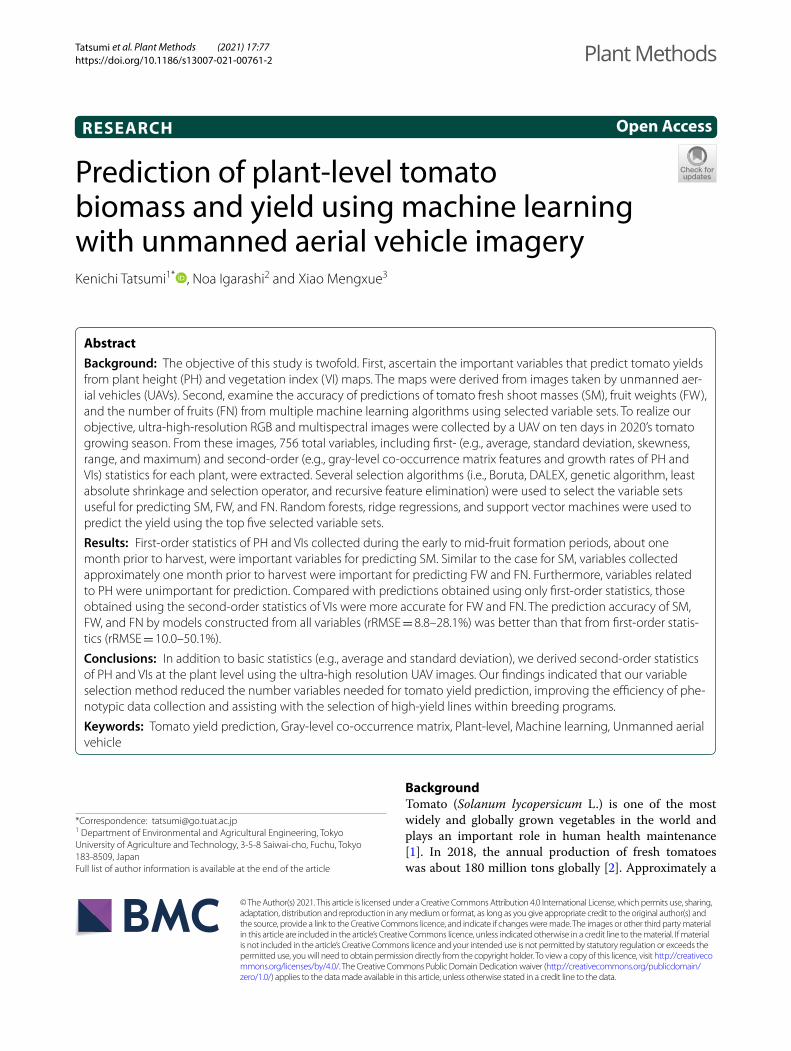
Data acquisition by UAVA gimbal-stabilized Zenmuse X5S camera (DJI Co., Ltd., Shenzhen, China) and multispectral image sensor cam-era Altum (MicaSense Co., Ltd., SEA, USA) mounted on a DJI Matrice 210 V2 (DJI Co., Ltd., Shenzhen, China) were used to collect the aerial RGB imagery and multi-spectral images using six bands (blue: 475 nm center, green: 560 nm center, red: 668 nm center, red edge: 717 nm center, near infrared: 842 nm center, and thermal infrared: 8–14 μm). The sensor resolution of each RGB megapixel and individual spectral image (except ther-mal infrared) was 5280 × 3956 and 2064 × 1554 pixels, respectively. The flight height was 12 m above ground to extract the features of each plant with ultra-high reso-lution and without being affected by wind caused by the UAV, and the forward and side overlaps were set as

90% and 70%, respectively. The RGB imagery and mul-tispectral reflectance image data were acquired on May 24, May 30, June 5, June 11, June 18, June 26, July 2, July 12, July 16, and July 24. Both types of image data were obtained between 10:00 and 11:00 local time. Aerial mul-tispectral images were radiometrically calibrated with a MicaSense’s Calibrated Reflectance Panel and MicaSense downwelling light sensor mounted on top of the UAV facing up towards the sky (Fig. 2). The reflectance val-ues of the calibrated panel across blue, green, red, near infrared reflectance (nir), and red edge were 0.528, 0.531, 0.531, 0.529, and 0.531, respectively.

Flight parameter settings, including flight path, were designated using the flight planning software Pix4Dcap-ture (Pix4D S.A., Lausanne, Switzerland), and the ground sampling distance was 0.3 cm/pixel for RGB images and 0.52 cm/pixel for spectral images. Each sensor acquired 80 RGB and 400 spectral images on average per flight.

Fig. 1 Experimental field used in this study. Field is located in Tokyo, Japan. This orthomosaic image was created using unmanned aerial vehicle images taken on June 18

Fig. 2 The UAV and sensor system utilized


Ground control points, for which we used a black and white cross-centered board, were placed at each of the four corners of the target field. Geometric calibration was conducted during the orthomosaic imagery process in Pix4Dmapper Pro version 4.6.3 (Pix4D S.A., Lausanne, Switzerland) using the ground control points. Digital surface model (DSM), which represents the elevation of plant structures, was created by Pix4Dmapper automati-cally. The digital terrain model (DTM) which represents the elevation of the soil surface, was estimated by inter-polating segmented soil pixels. In this study, the thresh-old value for segmenting soil and vegetation pixels was set to NDVI = 0.1. For multispectral images, radiometric calibration was performed in Pix4Dmapper during the orthorectification process using the calibration data by panel reflectance values collected during the flight with the downwelling light sensor. Finally, the reflectance map of six-band with GeoTIFF format was obtained automati-cally using Pix4Dmapper.

Yield surveySM, FW, and FN of individual plants in the tomato field were harvested on July 29 and July 30. These yield com-ponents were used for variable selection, prediction model training, and prediction accuracy analysis.

PH and VI calculationPH maps were calculated by subtracting the DTM from the DSM. The three VIs typically used for measurements of leaf chlorophyll content, plant height, biomass, and crop growth indicators [9, 30–32] were calculated from the multispectral maps: green normalized difference vegetation index (GNDVI) [33], normalized difference vegetation index (NDVI) [34], and weighted difference vegetation index (WDVI) [35]. We selected these three VIs because (1) the use of several types of VIs is not nec-essarily efficient as time-series analysis takes time, and high correlation coefficients among the VIs causes mul-ticollinearity; (2) NDVI and GNDVI are correlated with

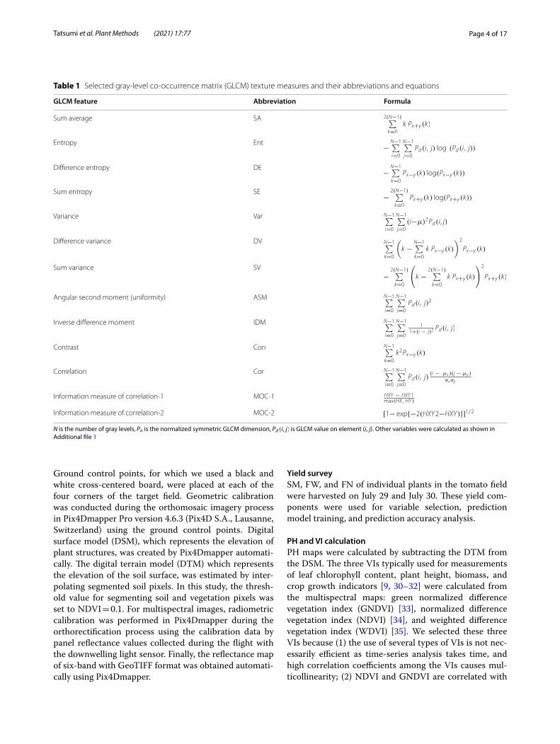
Table 1 Selected gray-level co-occurrence matrix (GLCM) texture measures and their abbreviations and equations

N is the number of gray levels, Pd is the normalized symmetric GLCM dimension, Pd(i, j) is GLCM value on element (i, j). Other variables were calculated as shown in Additional file 1

GLCM feature Abbreviation Formula

Sum average SA 2(N−1)∑

k=0

k Px+y(k)

Entropy Ent−

N−1∑

i=0

N−1∑

j=0

Pd(i, j) log (Pd(i, j))

Difference entropy DE−

N−1∑

k=0

Px−y(k) log(Px−y(k))

Sum entropy SE−

2(N−1)∑

k=0

Px+y(k) log(Px+y(k))

Variance Var N−1∑

i=0

N−1∑

j=0

(i−µ)2Pd(i, j)

Difference variance DV N−1∑

k=0

(

k −N−1∑

k=0

k Px−y(k)

)2

Px−y(k)

Sum variance SV−

2(N−1)∑

k=0

(

k −2(N−1)∑

k=0

k Px+y(k)

)2

Px+y(k)

Angular second moment (uniformity) ASM N−1∑

i=0

N−1∑

j=0

Pd(i, j)2

Inverse difference moment IDM N−1∑

i=0

N−1∑

j=0

11+(i − j)2

Pd(i, j)

Contrast Con N−1∑

k=0

k2Px−y(k)

Correlation Cor N−1∑

i=0

N−1∑

j=0

Pd(i, j)(i − µx )(j − µy )

σxσy

Information measure of correlation-1 MOC-1 HXY − HXY1max(HX , HY)

Information measure of correlation-2 MOC-2 [1− exp{−2(HXY2−HXY)}]1/2


leaf chlorophyll content and are widely used for yield pre-dictions [9, 30–32]; 3) WDVI can take into account the soil background influences.

(1)GNDVI = (NIR−Green)/(NIR+Green).

(2)NDVI = (NIR−Red)/(NIR+ Red).

(3)WDVI = NIR−a× Red.

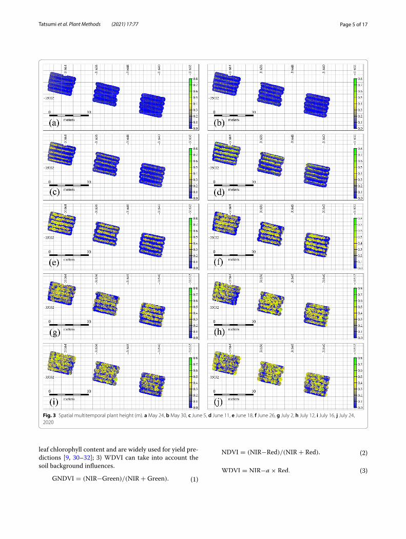
Fig. 3 Spatial multitemporal plant height (m). a May 24, b May 30, c June 5, d June 11, e June 18, f June 26, g July 2, h July 12, i July 16, j July 24, 2020


Here, NIR is crop reflectance in the near infrared band, Green is crop reflectance in the green band, Red is crop reflectance in the red band, and a is the slope of the soil line.

Variable extraction from PH and VI mapsIn order to extract the variables that may be related to the tomato biomass and yield of each plant, the following preprocessing was performed on the PH and VI maps.

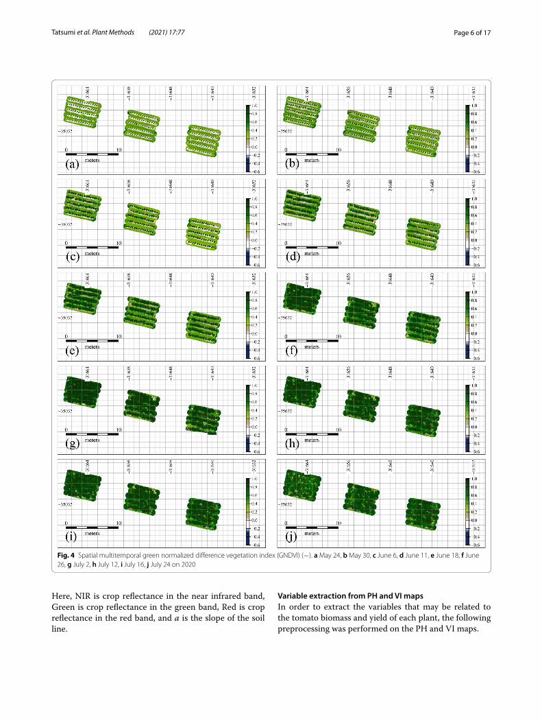
Fig. 4 Spatial multitemporal green normalized difference vegetation index (GNDVI) (−). a May 24, b May 30, c June 6, d June 11, e June 18, f June 26, g July 2, h July 12, i July 16, j July 24 on 2020


(1) Extraction of plant part: Tomato plant parts for each plant were extracted from the pixels with NDVI > 0.5 using the orthomosaic photo image from May 14. Some pixels identified as weeds were manually removed.

(2) Centroid determination of each plant: Using the closed vector line of each plant sample obtained in step 1, the centroid of each plant was determined.

(3) Region of interest (ROI) extraction of each plant: To calculate the feature variables for each plant, a circle with a radius of 20 cm centered on the centroid of each plant estimated in steps 1 and 2 was extracted as ROI.

In the present study, pixel statistics and dynamic growth rate were extracted as candidates for explanatory variables. In the ROI of each plant, five first-order statis-tics (average (AVE), standard deviation (SD), skewness (SKEW), range (RANGE), and maximum (MAX)) were extracted as basis statistics from PH and VI maps. Next, thirteen second-order statistics, which only considered the spatial pattern based on gray-level co-occurrence matrix (GLCM) [36], sum average (SA), entropy (Ent),

different entropy (DE), sum entropy (SE), variance (Var), difference variance (DV), sum variance (SV), angular sec-ond moment (ASM), inverse difference moment (IDM), contrast (Con), correlation (Cor), and information meas-ures of correlation (MOC-1, MOC-2) were derived from PH and VIs maps as GLCM features. Table 1 shows cal-culation formulas of the 13 extracted feature texture metrics. Next, dynamic average growth rates of PH and VIs were included as second-order statistics in this study and were considered as explanatory variables. In this study, growth rates were calculated for each plot as the change of PH and VIs over two consecutive measure-ment days divided by the measurement interval. As a result, a total of 756 variables (18 features (first- and sec-ond-order statistics) × 10 dates od PH (180 variables); 18 features × 10 days of three VIs (540 variables); 9 dynamic growth rates from PH (9 variables); 9 dynamic growth rates from three VIs (27 variables)) were extracted for variable selection.

Variable selection for tomato yield predictionTo reduce computational complexity, promote efficient data analysis and data understanding, determine critical

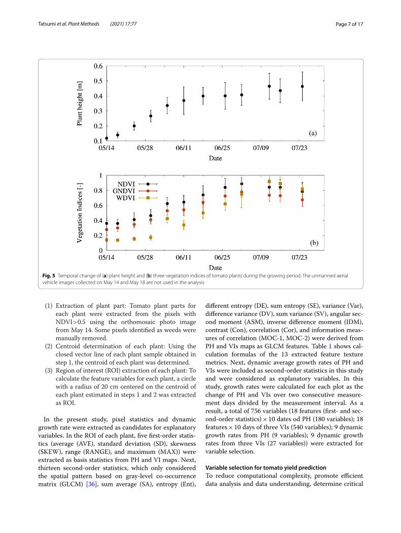
Fig. 5 Temporal change of (a) plant height and (b) three vegetation indices of tomato plants during the growing period. The unmanned aerial vehicle images collected on May 14 and May 18 are not used in the analysis


phenotypic traits or growth stages, variable selection methods involve evaluating important phenotypic traits on yield. In addition, variable selection is a fundamental step in ML algorithm and regression modeling. In the present study, the two groups of extracted variables, a total of 200 (5 first-order statistics × 10 dates for PH and 3 VI maps) and all 756 available variables, were handled as candidates in variable selection methods to explain tomato SM, FW, and FN. The reason we prepared two groups of variables is to determine if there is a difference in the prediction accuracy of tomato biomass and yield when using only basic statistics and all 756 variables as candidates. After generating first- and second-order sta-tistics and dynamic growth rates from PH and VI maps, normalization was conducted before each variable

selection procedure as preprocessing. Next, we applied five effective and powerful variable selection techniques to extract candidate variables. These were Boruta [37], DALEX [38], genetic algorithm (GA) [39], least abso-lute shrinkage and selection operator (LASSO) [40], and recursive feature elimination (RFE) [41].

Boruta is a non-parametric feature ranking and selec-tion algorithm based on random forest algorithms that can decide if a variable is important and contributes to selection of statistically significant confirmed variables. DALEX is a potent non-parametric tool that explains var-ious attributes such as implemented loss functions about the variables used in a machine learning model. GA is a non-parametric stochastic method for function optimi-zation based on the mechanics of natural genetics and

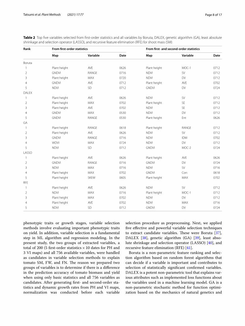
Table 2 Top five variables selected from first-order statistics and all variables by Boruta, DALEX, genetic algorithm (GA), least absolute shrinkage and selection operator (LASSO), and recursive feature elimination (RFE) for shoot mass (SM)

Rank From first-order statistics From first- and second-order statistics

Map Variable Date Map Variable Date

Boruta

1 Plant height AVE 0626 Plant height MOC-1 0712

2 GNDVI RANGE 0716 NDVI SV 0712

3 Plant height MAX 0720 NDVI DV 0712

4 GNDVI AVE 0712 Plant height AVE 0702

5 NDVI SD 0712 GNDVI DV 0724

DALEX

1 Plant height AVE 0626 NDVI SV 0712

2 Plant height MAX 0702 Plant height SE 0712

3 Plant height AVE 0702 NDVI SE 0712

4 GNDVI MAX 0530 NDVI DV 0712

5 GNDVI RANGE 0530 Plant height Ent 0626

GA

1 Plant height RANGE 0618 Plant height RANGE 0712


3 GNDVI RANGE 0716 NDVI IDM 0702

4 WDVI MAX 0724 NDVI DV 0712

5 NDVI SD 0712 GNDVI MOC-2 0724

LASSO

1 Plant height AVE 0626 Plant height AVE 0626

2 GNDVI RANGE 0716 GNDVI DV 0724

3 NDVI MAX 0716 NDVI SV 0716

4 Plant height MAX 0702 GNDVI Con 0618

5 Plant height SKEW 0605 Plant height MAX 0702

RFE


2 NDVI MAX 0716 Plant height MOC-1 0712

3 Plant height MAX 0702 NDVI DV 0712

4 Plant height AVE 0702 NDVI MAX 0716

5 NDVI SD 0712 GNDVI DV 0724


biological evolution. LASSO is a method of automatic parametric variable selection that eventually reduces the coefficients of certain unwanted features to zero due to penalization with L1-norm and minimizes the predic-tion error. RFE is a non-parametric feature selection that fits a model and removes the weakest feature until the specified number of features is reached. Furthermore, it attempts to eliminate dependencies and collinearity that may exist in the model. All variable selection processes were conducted using R (Version 3.6.3).

In this study, top five variables with the highest impor-tance scores were selected as useful in predicting tomato SM, FW, and FN by five variable selection methods. Each of the variable groups selected from 200 and 756 vari-ables were used as input for random forest (RF), ridge

regression (RI), and support vector machine (SVM) in R to predict SM, FW, and FN. RF model is a machine learning method that can be used for a variety of tasks including classification and regression. It consists of a large number of decision trees and combines the predic-tors of the estimators to produce a more accurate predic-tion [42]. RI model is a technique for analyzing multiple regression data that suffer from multicollinearity, and it performs L2 regularization [43–45]. SVM model is a supervised machine learning algorithm that is used for classification, regression, and detection of outliers and is capable of addressing the collinearity issue [46]. Hyperparameters for RF, RI, and SVM were optimized using “tuneRF” function in randomForest package, ten-fold cross validation, and “tune svm” functions in e1071

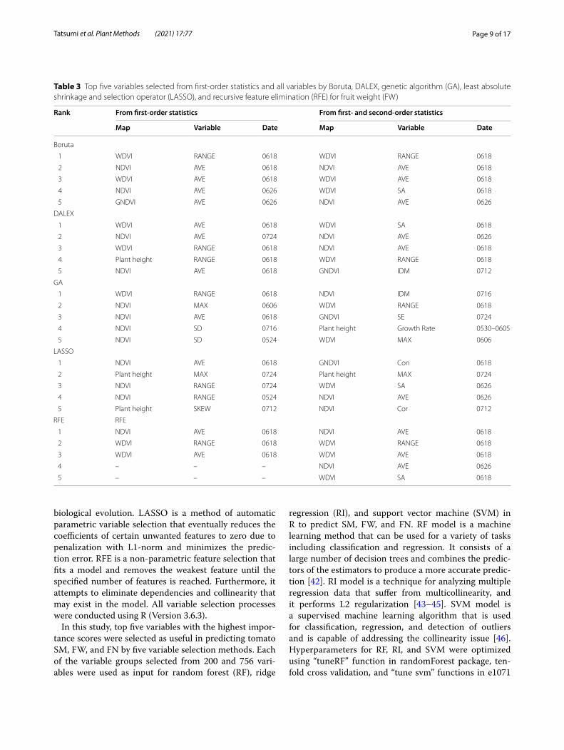
Table 3 Top five variables selected from first-order statistics and all variables by Boruta, DALEX, genetic algorithm (GA), least absolute shrinkage and selection operator (LASSO), and recursive feature elimination (RFE) for fruit weight (FW)



Boruta

1 WDVI RANGE 0618 WDVI RANGE 0618

2 NDVI AVE 0618 NDVI AVE 0618

3 WDVI AVE 0618 WDVI AVE 0618

4 NDVI AVE 0626 WDVI SA 0618

5 GNDVI AVE 0626 NDVI AVE 0626

DALEX

1 WDVI AVE 0618 WDVI SA 0618


3 WDVI RANGE 0618 NDVI AVE 0618

4 Plant height RANGE 0618 WDVI RANGE 0618

5 NDVI AVE 0618 GNDVI IDM 0712

GA

1 WDVI RANGE 0618 NDVI IDM 0716

2 NDVI MAX 0606 WDVI RANGE 0618

3 NDVI AVE 0618 GNDVI SE 0724

4 NDVI SD 0716 Plant height Growth Rate 0530–0605

5 NDVI SD 0524 WDVI MAX 0606

LASSO

1 NDVI AVE 0618 GNDVI Con 0618

2 Plant height MAX 0724 Plant height MAX 0724

3 NDVI RANGE 0724 WDVI SA 0626

4 NDVI RANGE 0524 NDVI AVE 0626

5 Plant height SKEW 0712 NDVI Cor 0712

RFE RFE


2 WDVI RANGE 0618 WDVI RANGE 0618

3 WDVI AVE 0618 WDVI AVE 0618

4 – – – NDVI AVE 0626

5 – – – WDVI SA 0618


package, respectively. To evaluate the model perfor-mance, 80% of all observation data were used as train-ing data and the remaining 20% was used for the model evaluation. The prediction performance of each model was evaluated using coefficient of determination (R2) and relative root mean square error (rRMSE).

Results and discussionTemporal change of PH and VIsMultitemporal UAV-derived data allow the quantitative evaluation of tomato growth with PH and VIs using DSM, DTM, and multispectral reflectance images. Figures 3 and 4 show the multitemporal growth change of PH and GNDVI, respectively, during the growing period in the

entire field. Additional file 2: Figures S1 and S2 indicate the multitemporal maps of NDVI and WDVI, respec-tively. Yellower and greener pixels in Figs. 3 and 4, Addi-tional file 2: Figures S1 and S2 mean taller PH and tomato vigor, respectively. PH increased linearly until flowering [around 160 DOY (day of year)]; after that, although the leaves spread horizontally, PH grew at a very small rate and remained almost unchanged during mature fruiting. In contrast, NDVI and GNDVI peaked on 184 DOY, and WDVI peaked on 194 DOY (Fig. 5). The growth trend of PH, which is a sigmoid curve, was also found in other research [47]. In addition, the phenomenon that VIs begin to decline at the end of the growing period is due to the leaf aging and yellowing. In summary, relatively large growth rate of PH and small growth rate of VIs were

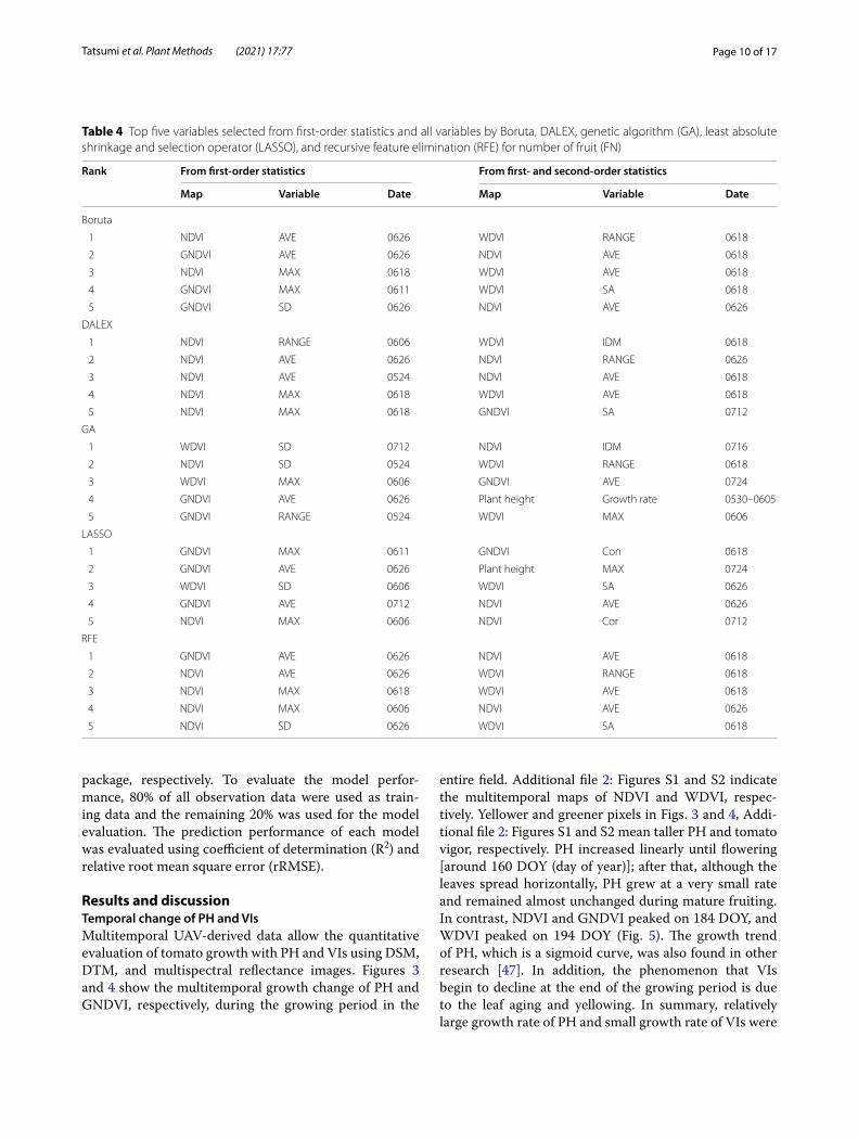
Table 4 Top five variables selected from first-order statistics and all variables by Boruta, DALEX, genetic algorithm (GA), least absolute shrinkage and selection operator (LASSO), and recursive feature elimination (RFE) for number of fruit (FN)



Boruta

1 NDVI AVE 0626 WDVI RANGE 0618


3 NDVI MAX 0618 WDVI AVE 0618

4 GNDVI MAX 0611 WDVI SA 0618

5 GNDVI SD 0626 NDVI AVE 0626

DALEX

1 NDVI RANGE 0606 WDVI IDM 0618

2 NDVI AVE 0626 NDVI RANGE 0626



5 NDVI MAX 0618 GNDVI SA 0712

GA

1 WDVI SD 0712 NDVI IDM 0716

2 NDVI SD 0524 WDVI RANGE 0618

3 WDVI MAX 0606 GNDVI AVE 0724

4 GNDVI AVE 0626 Plant height Growth rate 0530–0605

5 GNDVI RANGE 0524 WDVI MAX 0606

LASSO

1 GNDVI MAX 0611 GNDVI Con 0618

2 GNDVI AVE 0626 Plant height MAX 0724

3 WDVI SD 0606 WDVI SA 0626


5 NDVI MAX 0606 NDVI Cor 0712

RFE


2 NDVI AVE 0626 WDVI RANGE 0618


4 NDVI MAX 0606 NDVI AVE 0626

5 NDVI SD 0626 WDVI SA 0618


found until flowering date (mid-June); subsequently, the growth rate of PH slowed down and the growth rates of VIs increased. The ripening stage was characterized by a decrease in the VIs.

Variable selectionTables 2, 3, and 4 show the selected top five variables according to averaged importance score estimated by Boruta, DALEX, GA, LASSO, and RFE for SM, FW, and FN, respectively. As for SM, first- and second-order

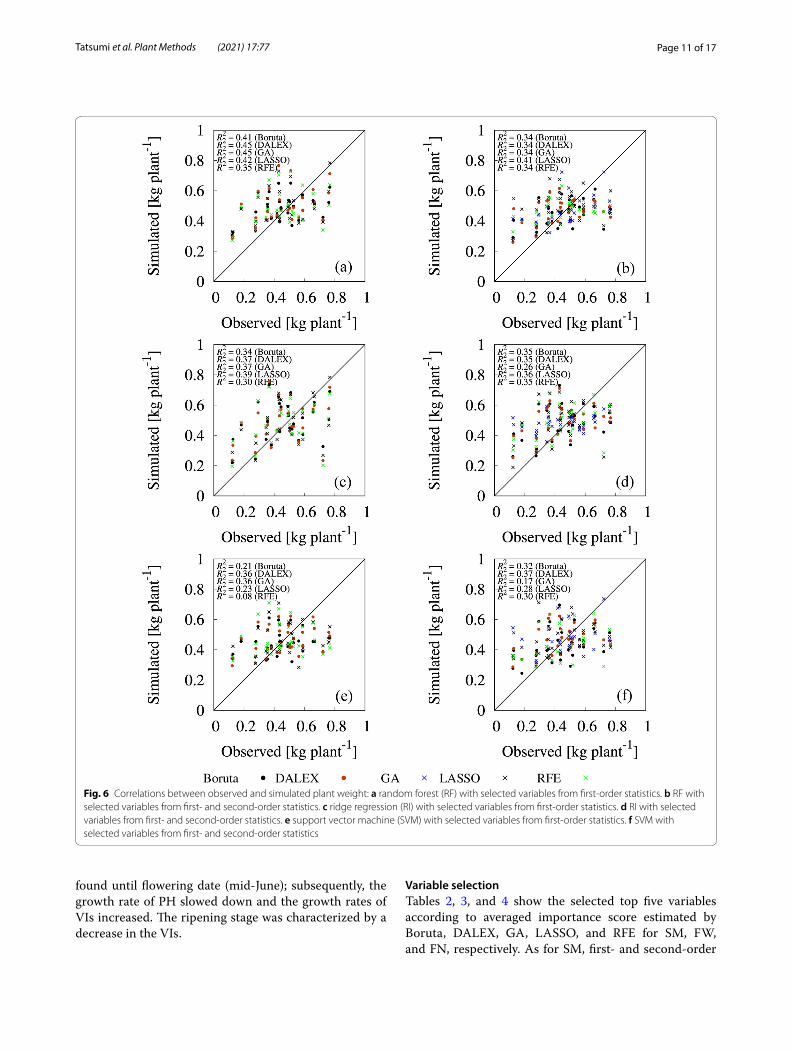
Fig. 6 Correlations between observed and simulated plant weight: a random forest (RF) with selected variables from first-order statistics. b RF with selected variables from first- and second-order statistics. c ridge regression (RI) with selected variables from first-order statistics. d RI with selected variables from first- and second-order statistics. e support vector machine (SVM) with selected variables from first-order statistics. f SVM with selected variables from first- and second-order statistics


statistics related to PH and VIs during mid-fruit forma-tion stage (from late-June to mid-July) were selected by all variable selection methods. AVE and MAX of PH and RANGE of GNDVI selected from extracted first-order

statistics, and SV and DV of NDVI selected from all sta-tistics were ranked in top five by all variable selection methods (Table 2). Moreover, other second-order statis-tics features such as MOC-1, DV, SE, Entr, IDM, MOC-2,

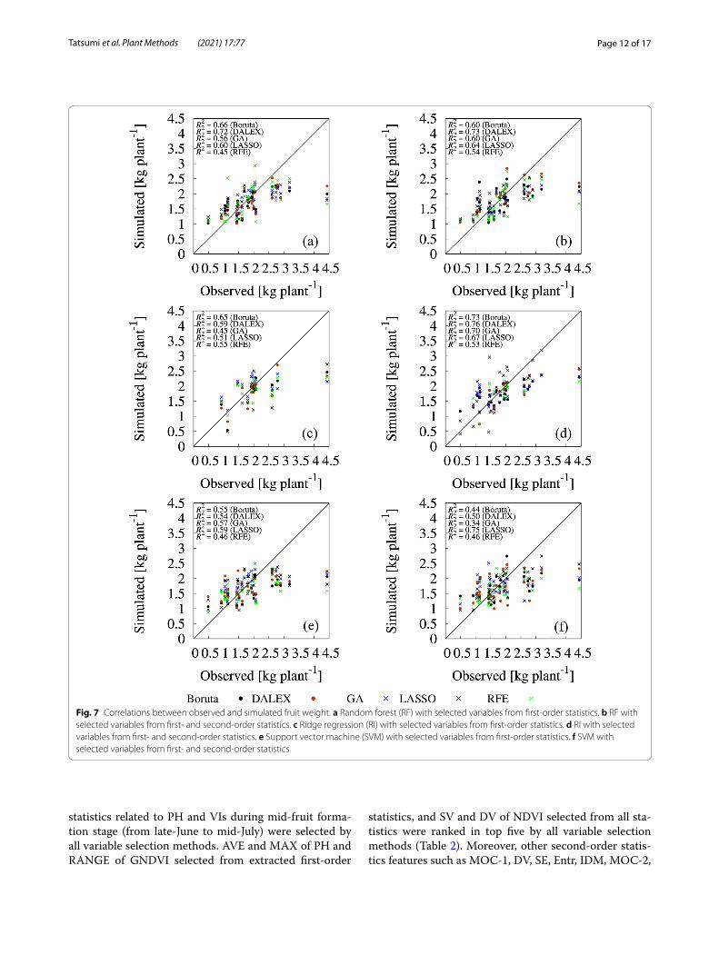
Fig. 7 Correlations between observed and simulated fruit weight. a Random forest (RF) with selected variables from first-order statistics. b RF with selected variables from first- and second-order statistics. c Ridge regression (RI) with selected variables from first-order statistics. d RI with selected variables from first- and second-order statistics. e Support vector machine (SVM) with selected variables from first-order statistics. f SVM with selected variables from first- and second-order statistics


and Con were also ranked as selected variables. Selected first- and second-order statistics of VIs and PH from extracted basic and all variables describe homogeneity and heterogeneity in the entire field. Although basic sta-tistics and GLCM features of PH and VIs are important

for SM estimation, all variable selection methods selected more PH-related variables after flowering compared with results of FW and FN. Although these results may vary depending on the employed explanatory variables and the variable selection method, in this study, the importance

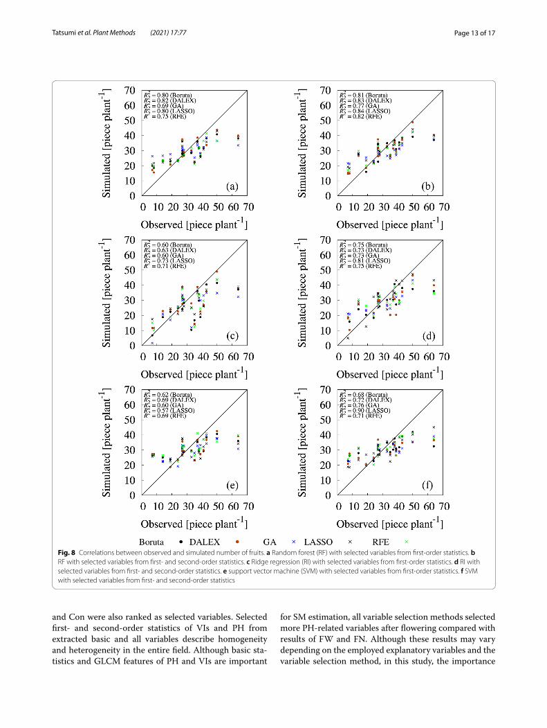
Fig. 8 Correlations between observed and simulated number of fruits. a Random forest (RF) with selected variables from first-order statistics. b RF with selected variables from first- and second-order statistics. c Ridge regression (RI) with selected variables from first-order statistics. d RI with selected variables from first- and second-order statistics. e support vector machine (SVM) with selected variables from first-order statistics. f SVM with selected variables from first- and second-order statistics


of PH in SM estimation was confirmed. Prediction of SM is important for estimating the assimilation potential by leaf photosynthesis. Therefore, the relationship of PH and SM has been an interesting issue for researchers and breeders. It was potentially shown that the variables of PH and VIs in the later growth period were significant for the final SM estimation.

In contrast, most selected variables by all variable selection models for FW were VI-related variables. RANGE of WDVI on June 18 selected by Boruta, DALEX, GA, and RFE from basic and all variables was ranked in top five variables (Table 3). Moreover, AVE of NDVI was also ranked in top five variables by all variable selection models except for GA from all avail-able variables. Interestingly, the results show that VI variables about one month prior to harvest are criti-cal for estimating FW. The finding that the VIs at the onset of fruiting are determinants of the final FW can

be relevant for field management. Similar to FW, FN is an important factor for determining yield. Tech-nology to estimate the FN on each plant, which is not visible in aerial images, can contribute to cultivation management. Although the selected variables by vari-able selection methods are different, AVE of NDVI or WDVI was selected in top five variables from both basic and all available variables (Table 4). In addition, it can be seen that the first- and second-order statis-tics of VIs on early to mid-fruit formation period are useful for estimating FN. However, unlike with SM, PH-related variables were found to be unnecessary variables for estimating FN.

Tomato yield prediction by models using selected variablesRF, RI, and SVM were built by using 80% (n = 120) of the data for training with a total of five sets of selected

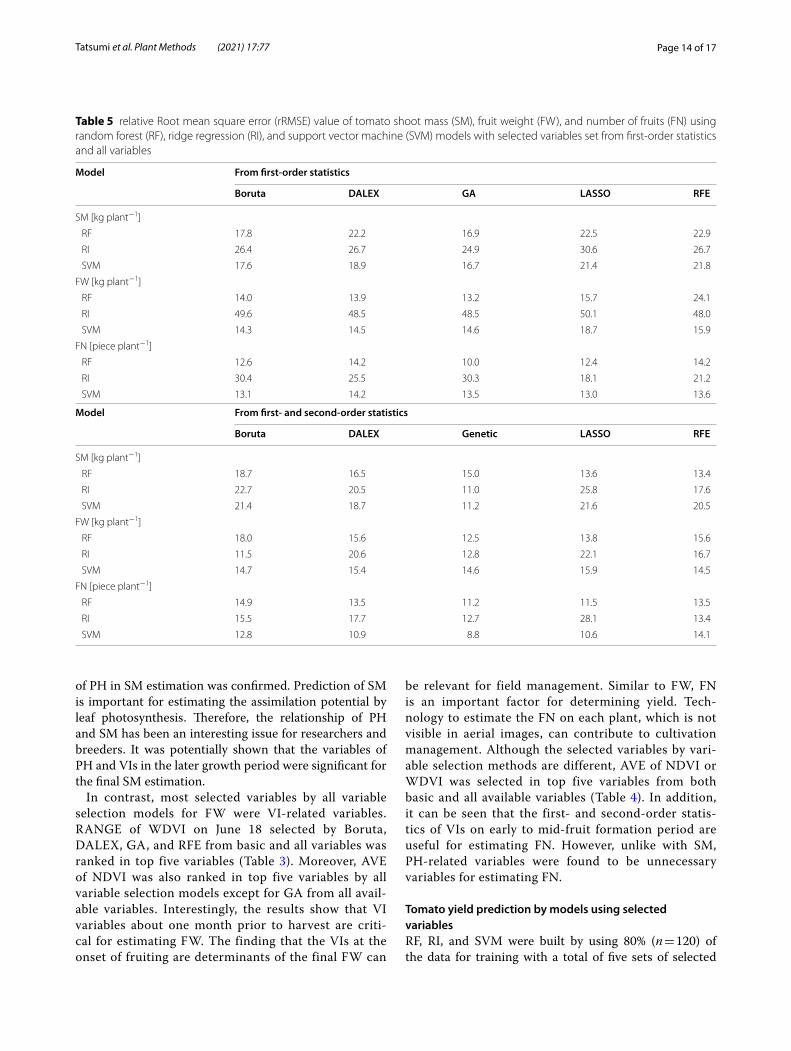
Table 5 relative Root mean square error (rRMSE) value of tomato shoot mass (SM), fruit weight (FW), and number of fruits (FN) using random forest (RF), ridge regression (RI), and support vector machine (SVM) models with selected variables set from first-order statistics and all variables

Model From first-order statistics

Boruta DALEX GA LASSO RFE

SM [kg plant−1]

RF 17.8 22.2 16.9 22.5 22.9

RI 26.4 26.7 24.9 30.6 26.7

SVM 17.6 18.9 16.7 21.4 21.8

FW [kg plant−1]

RF 14.0 13.9 13.2 15.7 24.1

RI 49.6 48.5 48.5 50.1 48.0

SVM 14.3 14.5 14.6 18.7 15.9

FN [piece plant−1]

RF 12.6 14.2 10.0 12.4 14.2

RI 30.4 25.5 30.3 18.1 21.2

SVM 13.1 14.2 13.5 13.0 13.6

Model From first- and second-order statistics

Boruta DALEX Genetic LASSO RFE

SM [kg plant−1]

RF 18.7 16.5 15.0 13.6 13.4

RI 22.7 20.5 11.0 25.8 17.6

SVM 21.4 18.7 11.2 21.6 20.5

FW [kg plant−1]

RF 18.0 15.6 12.5 13.8 15.6

RI 11.5 20.6 12.8 22.1 16.7

SVM 14.7 15.4 14.6 15.9 14.5

FN [piece plant−1]

RF 14.9 13.5 11.2 11.5 13.5

RI 15.5 17.7 12.7 28.1 13.4

SVM 12.8 10.9 8.8 10.6 14.1


important variables. The performance of constructed models was evaluated using the remaining 20% for test-ing by tenfold cross validation. Figures 6, 7, and 8 show the relationship between observed and simulated SM, FW, and FN using RF, RI, and SVM models with the selected variables set, respectively. Table 5 indicates rRMSE between the observed and simulated values by RF, RI, and SVM models with the five sets of selected var-iables, reflecting the prediction accuracy of the validated model with test data.

Comparing among the five different variable sets for SM prediction, variable sets from first-order statistics selected by Boruta and DALEX had better goodness of fit with RF model (R2 = 0.41 for Boruta; R2 = 0.45 for DALEX) (Fig. 6a) than the other combinations of vari-able selection method and prediction model. In the rRMSE, GA-selected variable set from all variables with RI and SVM had smaller absolute error of a model (rRMSE = 11.0% for RI; rRMSE = 11.2% for SVM). For SM prediction, RF with selected variable sets from first-order basic statistics had better performance in R2; whereas second-order statistics decreased the rRMSE value for many combinations of prediction models and variable selection methods (Table 5). For the compari-son with R2, it was an interesting result that prediction of SM does not require the GLCM texture information, and only the first-order statistics are sufficient to obtain the certain prediction accuracy.

Regarding FW, the following combinations had supe-rior performance among the variable sets and pre-diction models combinations: Boruta-, DALEX-, and GA-selected variable sets from all variables with RI (R2 = 0.73, 0.76, and 0.70, respectively) (Fig. 7d), LASSO-selected variable set from all variables with SVM (R2 = 0.75) (Fig. 7f ), and RFE-selected variable set from first-order statistics variables with RI (R2 = 0.55) (Fig. 7c). In particular, focusing on the RI, the prediction accuracy of the models, except RFE, with the selected variables using all variables was greatly improved compared with that using selected variable set from first-order statistics only. For example, GA-selected variable set from first-order statistics with RI model had lower R2 value (0.45), whereas that from all variables had higher R2 value (0.70). IDM of NDVI from all variables was ranked as top one variable by GA (Table 3). IDM feature relates inversely to the contrast measure and is a direct measure of the local homogeneity of a digital image. Therefore, this result shows the importance of second-order statistics for predicting FW. For FN prediction, simulated value with selected variable sets from all variables by all prediction models had significantly higher goodness of fit compared with selected variable sets from first-order statistics. In particular, Boruta-, DALEX-, GA-, and RFE-selected

important variable sets with RF (Fig. 8b), and LASSO-selected feature variable sets with SVM (Fig. 8f ) achieved higher prediction performances compared with the other combinations of selected feature variable sets and predic-tion models (R2 = 0.81 for Boruta; R2 = 0.83 for DALEX; R2 = 0.82 for RFE; R2 = 0.77 for GA; R2 = 0.82 for RFE; R2 = 0.90 for LASSO).

In the present study, RF with Boruta-selected variable set from first-order statistics, RI with DALEX-selected variable set from all variables, and SVM with LASSO-selected variable set from all variables had best predic-tion performance R2 with the observed SM, FW, and FN, respectively. Although it is difficult to make simple comparisons due to the differences of cultivation envi-ronments, varieties, and extracted variables, Li et al. [48] suggested that non-parametric (parametric) pre-diction model is adopted to match the non-parametric (parametric) variable selection. In this study, there were no clear effect relationships between parametric (non-parametric) variable selection method and parametric (non-parametric) model on tomato yield prediction accuracy. Furthermore, prediction accuracy of FW and FN using the selected variable set from all variables was significantly better compared with that using selected variable set from first-order statistics. Moreover, statis-tic variables of the VIs about one month before harvest were found to be important in predicting tomato yield.

Narrowing the focus to secondary traits and growth stages that affect tomato yield will contribute to more effective phenotypic data collection. In addition, the super-high-resolution field images obtained from the UAV provided helpful traits, such as temporal change of plant height and vegetation indices including sec-ondary-order statistics of the field. Although we only used these three VIs in this study, we intend to use more VIs, including blue, red edge, and thermal bands, to predict the yield in the near future. Our next goal is to extract the features necessary to build a robust prediction model by testing the proposed variable selection with more data collected in multipoint and multiple years and thus contribute to the efficient selec-tion of high-yield lines in breeding process.

ConclusionIn this study, we sought to examine the prediction accuracy of SM, FW, and FN using RF, RI, and SVM using variable sets selected by Boruta, DALEX, GA, LASSO, and RFE. PH and VIs (NDVI, GNDVI, and WDVI) from UAV-derived imagery were used for extraction of first-order basic statistics and second-order statistics (GLCM features and dynamic growth rate). First-order statistics of PH and VIs at early to mid-fruit formation period were ranked as important


variables for prediction of SM by all feature selection methods. GLCM features of NDVI and WDVI from June 18 were significantly important for prediction of FW. Similar to FW prediction, GLCM features of VIs one month before harvest were significant to pre-dict FN. Furthermore, all prediction models with the selected variable sets from all variables achieved good performance for FW and FN prediction compared with selected variable sets using basic statistics only. In par-ticular, RF with Boruta-selected variable set from the basic statistics, RI with DALEX-selected variable set from all variables, and SVM with LASSO-selected vari-able set from all variables were best combinations for predicting SM, FW, and FN, respectively. These results indicate that filtering secondary traits and growth stages that contribute to the prediction of tomato yield can contribute to saving of time and labor required for phenotypic data collection and processing. In addi-tion, it is possible to obtain useful features for breeding, other than first-order basic statistics, such as second-order statistics in PH and VIs for each plant, from the ultra-high-resolution image obtained by UAV. Overall, our findings indicate that reduced features needed for tomato yield prediction by variable selection method will help improve the efficiency of phenotypic data col-lection and assist with the selection of high-yield lines in breeding programs.

In traditional machine learning techniques, it is diffi-cult to apply a trained model to other tomato cultivars or other crop species. In a future study, we will apply transfer learning techniques to extract the phenotype of different domains quantitatively using an expanded UAV dataset, and we will compare the results with those of the process in this study.

Supplementary InformationThe online version contains supplementary material available at https:// doi. org/ 10. 1186/ s13007- 021- 00761-2.

Additional file 1. Auxiliary formula for calculation of gray-level co-occurrence matrix (GLCM) features.

Additional file 2: Figure S1. Spatial multitemporal normalized difference vegetation index (NDVI) (−). Figure S2. Spatial multitemporal weighted difference vegetation index (WDVI) (−).

AcknowledgementsWe thank Shogo Takahashi and Makoto Niida from the Tokyo University of Agricultural and Technology, Japan, for their support with measurements.

Authors’ contributionsKT conceptualized the study, collected data, modelling, data analysis, wrote the paper—original draft. IN, and XM provided the field truth data. KT conducted the aerial data collections. KT, IN, and XM reviewed, edited, and finalized the paper. All authors have read and agreed to the published version of the manuscript. All authors read and approved the final manuscript.

FundingThis study was funded in part by JST PRESTO Grant Number JPMJPR1603, Japan, and JSPS KAKENHI Grant Number 16KK0169 and 19K15944.

Availability of data and materialsThe all datasets used analyzed in this study are available from the correspond-ing author on reasonable request.

Declarations

Ethics approval and consent to participateNot applicable.

Competing interestsNot applicable.

Author details1 Department of Environmental and Agricultural Engineering, Tokyo University of Agriculture and Technology, 3-5-8 Saiwai-cho, Fuchu, Tokyo 183-8509, Japan. 2 Faculty of Agriculture Tokyo University of Agriculture and Technology, 3-5-8 Saiwai-cho, Fuchu, Tokyo 183-8509, Japan. 3 Graduate School of Agricul-ture, Tokyo University of Agriculture and Technology, 3-5-8 Saiwai-cho, Fuchu, Tokyo 183-8509, Japan.

Received: 18 March 2021 Accepted: 4 June 2021

References 1. Li N, Wu X, Zhuang W, Xia L, Chen Y, Wu C, et al. Tomato and lyco-

pene and multiple health outcomes: umbrella review. Food Chem. 2021;343:128396.

2. FAO. FAOSTAT. http:// www. fao. org/ faost at/ en/# home. Accessed 18 Jan 2021.

3. Ramasamy S, Ravishankar M. Integrated pest management strategies for tomato under protected structures. In: Sustainable management of arthropod pests of tomato. Elsevier; 2018, pp. 313–322.

4. Islam J, Kabir Y. Effects and mechanisms of antioxidant-rich functional beverages on disease prevention. In: Functional and medicinal bever-ages. Elsevier; 2019, pp. 157–198.

5. Megan Ware RDNLD. Everything you need to know about tomatoes. https:// medil inkbl og. com/ every thing- you- need- to- know- about- tomat oes/. Accessed 27 Dec 2020.

6. Shi Y, Thomasson JA, Murray SC, Pugh NA, Rooney WL, Shafian S, et al. Unmanned aerial vehicles for high-throughput phenotyping and agronomic research. PLoS ONE. 2016;11(7):e0159781.

7. Barbedo JGA. A review on the use of unmanned aerial vehicles and imaging sensors for monitoring and assessing plant stresses. Drones. 2019;3(2):40.

8. Du M, Noguchi N. Monitoring of wheat growth status and mapping of wheat yield’s within-field spatial variations using color images acquired from UAV-camera system. Remote Sens. 2017;9(3):289.

9. Duan T, Chapman SC, Guo Y, Zheng B. Dynamic monitoring of NDVI in wheat agronomy and breeding trials using an unmanned aerial vehicle. Field Crop Res. 2017;210:71–80.

10. Senthilnath J, Dokania A, Kandukuri M, Ramesh KN, Anand G, Omkar SN. Detection of tomatoes using spectral-spatial methods in remotely sensed RGB images captured by UAV. Biosyst Eng. 2016;146:16–32.

11. Johansen K, Morton MJL, Malbeteau YM, Aragon B, Al-Mashharawi SK, Ziliani MG, et al. Unmanned aerial vehicle-based phenotyping using mor-phometric and spectral analysis can quantify responses of wild tomato plants to salinity stress. Front Plant Sci. 2019;10:370.

12. Johansen K, Morton MJL, Malbeteau Y, Aragon B, Al-Mashharawi S, Ziliani M, et al. Predicting biomass and yield at harvest of salt-stressed tomato plants using UAV imagery. Int Arch Photogramm Remote Sens Spatial Inf Sci. 2019;XLII-2/W13:407–11.

13. Candiago S, Remondino F, De Giglio M, Dubbini M, Gattelli M. Evaluat-ing multispectral images and vegetation indices for precision farming applications from UAV images. Remote Sens. 2015;7(4):4026–47.

https://doi.org/10.1186/s13007-021-00761-2

https://doi.org/10.1186/s13007-021-00761-2

http://www.fao.org/faostat/en/#home

https://medilinkblog.com/everything-you-need-to-know-about-tomatoes/

https://medilinkblog.com/everything-you-need-to-know-about-tomatoes/


• fast, convenient online submission

•

thorough peer review by experienced researchers in your field

• rapid publication on acceptance

• support for research data, including large and complex data types

•

gold Open Access which fosters wider collaboration and increased citations

maximum visibility for your research: over 100M website views per year •

At BMC, research is always in progress.

Learn more biomedcentral.com/submissions

Ready to submit your researchReady to submit your research ? Choose BMC and benefit from: ? Choose BMC and benefit from:

14. Enciso J, Avila CA, Jung J, Elsayed-Farag S, Chang A, Yeom J, et al. Valida-tion of agronomic UAV and field measurements for tomato varieties. Comput Electron Agric. 2019;158:278–83.

15. Holman F, Riche A, Michalski A, Castle M, Wooster M, Hawkesford M. High throughput field phenotyping of wheat plant height and growth rate in field plot trials using UAV based remote sensing. Remote Sens. 2016;8(12):1031.

16. Hu P, Chapman SC, Wang X, Potgieter A, Duan T, Jordan D, et al. Estima-tion of plant height using a high throughput phenotyping platform based on unmanned aerial vehicle and self-calibration: example for sorghum breeding. Eur J Agron. 2018;95:24–32.

17. Wang X, Singh D, Marla S, Morris G, Poland J. Field-based high-through-put phenotyping of plant height in sorghum using different sensing technologies. Plant Methods. 2018;14(1):53.

18. Fathipoor H, Arefi H, Shah-Hosseini R, Moghadam H. Corn forage yield prediction using unmanned aerial vehicle images at mid-season growth stage. J Appl Rem Sens. 2019;13(03):1.

19. Tattaris M, Reynolds MP, Chapman SC. A direct comparison of remote sensing approaches for high-throughput phenotyping in plant breeding. Front Plant Sci. 2016;7:1131.

20. Yang G, Liu J, Zhao C, Li Z, Huang Y, Yu H, et al. Unmanned aerial vehicle remote sensing for field-based crop phenotyping: current status and perspectives. Front Plant Sci. 2017;8:1111.

21. Ballesteros R, Ortega JF, Hernandez D, Moreno MA. Onion biomass moni-toring using UAV-based RGB imaging. Precision Agric. 2018;19(5):840–57.

22. Han L, Yang G, Dai H, Xu B, Yang H, Feng H, et al. Modeling maize above-ground biomass based on machine learning approaches using UAV remote-sensing data. Plant Methods. 2019;15(1):10.

23. Nevavuori P, Narra N, Lipping T. Crop yield prediction with deep convolu-tional neural networks. Comput Electron Agricult. 2019;163:104859.

24. Lu N, Zhou J, Han Z, Li D, Cao Q, Yao X, et al. Improved estimation of aboveground biomass in wheat from RGB imagery and point cloud data acquired with a low-cost unmanned aerial vehicle system. Plant Methods. 2019;15(1):17.

25. Jiang Q, Fang S, Peng Y, Gong Y, Zhu R, Wu X, et al. UAV-based biomass estimation for rice-combining spectral, TIN-based structural and mete-orological features. Remote Sens. 2019;11(7):890.

26. Yang Q, Shi L, Han J, Zha Y, Zhu P. Deep convolutional neural networks for rice grain yield estimation at the ripening stage using UAV-based remotely sensed images. Field Crop Res. 2019;235:142–53.

27. Escalante HJ, Rodríguez-Sánchez S, Jiménez-Lizárraga M, Morales-Reyes A, De La Calleja J, Vazquez R. Barley yield and fertilization analysis from UAV imagery: a deep learning approach. Int J Remote Sens. 2019;40(7):2493–516.

28. Moeckel T, Dayananda S, Nidamanuri R, Nautiyal S, Hanumaiah N, Buerk-ert A, et al. Estimation of vegetable crop parameter by multi-temporal UAV-borne images. Remote Sens. 2018;10(5):805.

29. Liakos K, Busato P, Moshou D, Pearson S, Bochtis D. Machine learning in agriculture: a review. Sensors. 2018;18(8):2674.

30. Kyratzis AC, Skarlatos DP, Menexes GC, Vamvakousis VF, Katsiotis A. Assess-ment of vegetation indices derived by UAV imagery for durum wheat

phenotyping under a water limited and heat stressed mediterranean environment. Front Plant Sci. 2017;8:1114.

31. Guan S, Fukami K, Matsunaka H, Okami M, Tanaka R, Nakano H, et al. Assessing correlation of high-resolution NDVI with fertilizer application level and yield of rice and wheat crops using small UAVs. Remote Sens. 2019;11(2):112.

32. Hassan MA, Yang M, Rasheed A, Yang G, Reynolds M, Xia X, et al. A rapid monitoring of NDVI across the wheat growth cycle for grain yield predic-tion using a multi-spectral UAV platform. Plant Sci. 2019;282:95–103.

33. Gitelson AA, Merzlyak MN. Remote sensing of chlorophyll concentration in higher plant leaves. Adv Space Res. 1998;22:689–92.

34. Rouse JW, Haas RH, Schell JA, Deering DW. Monitoring vegetation sys-tems in the great plains with ERTS. In: Third Earth Resources Technology Satellite (ERTS) Symposium, NASA SP-351; 1973. pp 309–317.

35. Qi J, Chehbouni A, Huete AR, Kerr YH, Sorooshian S. A modified soil adjusted vegetation index. Remote Sens Environ. 1994;48:119–26.

36. Haralick RM, Shanmugam K, Dinstein I. Textural features for image clas-sification. IEEE Trans Syst Man Cybern. 1973;SMC-3(6):610–21.

37. Kursa MB, Jankowski A, Rudnicki WR. Boruta—a system for feature selec-tion. Fund Inform. 2010;101(4):271–85.

38. Biecek P. DALEX: explainers for complex predictive models. J Mach Learn Res. 2018;19:1–14.

39. Scrucca L. GA: a package for genetic algorithms in R. J Stat Soft. 2013;53(4):1–37.

40. Tibshirani R. Regression shrinkage and selection via the lasso. J Roy Stat Soc: Ser B (Methodol). 1996;58(1):267–88.

41. Guyon I, Weston J, Barnhill S, Vapnik V. Gene selection for cancer classifica-tion using support vector machines. Mach Learn. 2002;46(1/3):389–422.

42. Breiman L. Random Forests. Mach Learn. 2001;45(1):5–32. 43. Hoerl AE, Kennard RW. Ridge regression: applications to nonorthogonal

problems. Technometrics. 1970;12(1):69–82. 44. Hoerl AE, Kennard RW. Ridge regression: biased estimation for non-

orthogonal problems. Technometrics. 1970;12(1):55–67. 45. de Vlaming R, Groenen PJF. The current and future use of ridge regression

for prediction in quantitative genetics. Biomed Res Int. 2015;2015:1–18. 46. Cortes C, Vapnik V. Support-vector networks. Mach Learn.

1995;20(3):273–97. 47. Esyanti RR, Dwivany FM, Almeida M, Swandjaja L. Physical, chemical and

biological characteristics of space flown tomato (Lycopersicum esculen-tum) seeds. J Phys Conf Ser. 2016;771:012046.

48. Li J, Veeranampalayam-Sivakumar A-N, Bhatta M, Garst ND, Stoll H, Stephen Baenziger P, et al. Principal variable selection to explain grain yield variation in winter wheat from features extracted from UAV imagery. Plant Methods. 2019;15(1):123.

Publisher’s NoteSpringer Nature remains neutral with regard to jurisdictional claims in pub-lished maps and institutional affiliations.

Documents

Prediction of plant-level tomato biomass and yield using