Pr

A T

rediction

Thesis Sub

D

NATION

n of Rel

Refere

mitted in P

M

Sh

DEPARTM

NAL INST

ative De

ence to C

Partial Fu

D

Master o

Civil E

huvransh

MENT OF

TITUTE O

Aug

ensity of

Compac

ulfillment 

egree of

of Technin

Engineer

hu Kuma 

F CIVIL E

OF TECH

gust, 2009

f Sand w

tion En

of the Re

nology

ring

ar Rout

ENGINEE

NOLOGY

9 

with Par

ergy

quiremen

ERING

Y ROURK

rticular

nts for the

KELA

e 

brought to you by COREView metadata, citation and similar papers at core.ac.uk

provided by ethesis@nitr

Pr

A T

rediction

Thesis Sub

Na

n of Rel

Refere

mitted in P

S

Depa

ational I

ative De

ence to C

Partial Fu

D

Master o

Civil E

Shuvransh

Under thProf.

rtment o

nstitute

Aug

ensity of

Compac

ulfillment 

egree of

of Technoin

Engineer

By

hu Kumar

he GuidancC. R. Pat

of Civil E

of Techn

gust 2009

f Sand w

tion En

of the Re

ology

ing

Rout

ce of tra

ngineeri

nology R

9

with Par

ergy

quiremen

ng

Rourkela

rticular

nts for thee 

This is

particula

partial fu

Engineer

him unde

To the be

other Un

Date:

to certify t

ar reference

fulfillment o

ring at Natio

er my superv

est of my kn

iversity / Ins

Natio

that the the

e to compa

of the requ

onal Institute

vision and gu

nowledge, th

stitute for th

onal InstiR

CER

esis entitled

ction energ

uirements fo

e of Techno

uidance.

he matter em

e award of a

itute of TeRourkela

RTIFICAT

d, “Predictio

gy” submitte

or the awar

ology, Rourk

mbodied in t

any Degree o

echnolog

TE

on of relat

ed by Mr Sh

rd of Maste

kela is an au

the thesis ha

or Diploma.

De Nationa R

gy

tive density

huvranshu

er of Techn

uthentic wor

as not been s

Dr. C. R Pa Professoept. of Civil

al Institute oRourkela – 7

y of sand

Kumar Rou

nology in

rk carried ou

submitted to

atra r l Engg. of Technolog769008

with

ut in

Civil

ut by

o any

gy

ACKNOWLEDGEMENT

I sincerely express my deep sense of gratitude to my thesis supervisor, Prof. Chittaranjan Patra

for his expert guidance, continuous encouragement and inspiration throughout the course of

thesis work. I am sincerely thankful for his intellectual support and creative criticism, which led

me to generate my own ideas and made my work interesting and enjoyable.

I would also like to express my deep appreciation and sincere thanks to Prof. M. Panda, Head,

Civil Engineering Department, Prof. N. R. Mohanty, Prof. N. Roy, Prof. S. P. Singh and Prof.

S. K. Das, of Civil Engineering for providing all kinds of possible help and encouragement. I am

indebted to all of them and NIT Rourkela for giving me the fundamentals and chance to

implement them.

The help and support received from Mr. Rabi Narayan Behera, Ph.D. Scholar, Civil Engineering

Department was vital for the success of the project.

I am also thankful to staff members of Geotechnical Engineering Laboratory especially Mr.

Chamuru Suniani & Mr. Kalakar Tanty for his assistance & cooperation during the course of

experimentation. I express my special thanks to my dear friends Mr. Biranchi Narayan Behera,

Mr. Suryakanta Sutar, Mr. Amrit Das and Mr. Chinmay Mohanty for their continuous support,

suggestions and love.

Friendly environment and cooperative company I had from my classmates and affection received

from my seniors and juniors will always remind me of my days as a student at NIT Rourkela. I

wish to thank all my friends and well wishers who made my stay at NIT Rourkela, memorable

and pleasant. I have no words to express my respect for my parents and my family members who

have been constant source of inspiration to me. Last but not the least; I am thankful to

ALMIGHTY, who kept me fit both mentally and physically through out the year for the project

work.

Shuvranshu Kumar Rout

Table of Contents

Abstract i

List of Tables ii

List of Figures iii

List of Abbreviations and Symbols iv

Chapter-1. Introduction 1

1.1 Background 1

Chapter-2. Literature Review 3

2.1 Theory of Relative Density 3

2.2 Theory of Compaction 7

2.2.1 Compaction Phenomenon 8

2.2.2 Field Compaction of Cohesionless Soils 10

2.3 Previous Work on Laboratory Density Test and Theoretical

Analysis

11

2.4 Motivation & Objective of Present Research Work 21

Chapter-3. Experimental Programme 22

3.1 Test Specimens 22

3.2 Test Methodology 22

3.2.1 Determination of Specific Gravity 22

3.2.2 Determination of Grain Size Distribution 23

3.2.3 Determination of Maximum Void Ratio 24

3.2.4 Determination of Minimum Void Ratio 25

3.2.5 Determination of Void Ratio corresponding to

Maximum Dry Density

26

3.2.6 Determination of Relative Density 29

Chapter-4. Results and Discussion 30

4.1 Index Properties of Sand 30

4.1.1 Prediction of maximum void ratio (emax) from mean

grain size (D50)

33

4.1.2 Prediction of minimum void ratio (emin) from mean

grain size (D50)

34

4.1.3 Prediction of void ratio range (emax - emin) from mean

grain size (D50)

35

4.1.4 Prediction of maximum void ratio (emax) from

minimum void ratio (emin)

36

4.1.5 Comparison of results of present study with previous

work

37

4.2 Relative density from standard and modified Proctor tests 42

4.2.1 Prediction of void ratio corresponding to standard

Proctor test (es) from mean grain size (D50)

45

4.2.2 Prediction of void ratio corresponding to modified

Proctor test (em) from mean grain size (D50)

46

4.2.3 Prediction of Relative Density (Dr) 47

4.2.4 Comparison of predicted relative density with

experimental values

51

4.3 Relative density from reduced standard and modified proctor 54

tests

4.3.1 Prediction of void ratio corresponding to reduced

standard Proctor test (ers) from mean grain size (D50)

57

4.3.2 Prediction of void ratio corresponding to reduced

modified Proctor test (erm) from mean grain size (D50)

58

4.3.3 Prediction of Relative Density (Dr) 59

4.3.4 Comparison of predicted relative density with

experimental values

63

4.4 Summary of results considering all the energy levels 66

4.4.1 Comparison of void ratios (emax, emin, es em, ers erm) 66

4.4.2 Empirical equations for void ratios (emax, emin, es em,

ers erm) at particular energy levels

67

4.4.3 Empirical equations for relative density (Dr) at

particular energy levels

68

4.4.4 Comparison of predicted relative density with

experimental values at different energy levels

69

4.4.5 Establishing relationship between relative density

(Dr) with mean grain size (D50) at different energy

levels

70

Chapter-5. Conclusions 72

Chapter-6. Scope of Further Study 73

References 74

Appendix - A. Figures 77

i

Abstract

Field compaction of sands usually involves different equipments with the compaction energy

varying significantly. The relative density is the better indicator for specifying the compaction of

granular soil. If the relative density can be correlated simply by any index property of the

granular soil, it can be more useful in the field. The relative density is defined in terms of voids

ratio. It is well known that the minimum and maximum voids ratio depend on the mean grain

size. However, there is no direct relation available for the voids ratio in terms of grain size.

Therefore, in this dissertation, the effect of mean grain size on the relative density of sand has

been studied at different compaction energies.

In order to arrive at the above, fifty five number of clean sands having D50 ranges from 0.34 to

2.6 mm collected from different river bed of Orissa have been tested in the laboratory. The

various index properties like grain specific gravity, grain size distribution of all the samples have

been determined. The minimum and maximum voids ratio have been determined. For

determining minimum voids ratio; both wet and dry method have been adopted. The voids ratio

corresponding to energy level of standard, modified, reduced standard, and reduced modified

Proctor tests have been correlated with mean grain size and thus the simple nonlinear empirical

relations have been developed. Similarly, the relative densities corresponding to the energy level

of above mentioned Proctor tests also have been correlated with mean grain size to arrive at

simple empirical equations. The percentage deviation of the relative density estimated by the

proposed method is in the range of ± 5 % of the measured value. The above correlations of

relative densities will be helpful for the design specifications in the field.

Key Words: Clean Sands, Compaction, Compaction Energy, Empirical Equations, Mean Grain

Size, Relative Density, Void Ratio.

ii

List of Tables

Table 2.1 Denseness of cohesionless soils 3

Table 3.1 Compaction energy for different proctor compaction tests 27

Table 4.1 Index properties of sand samples tested 30

Table 4.2 Experimental relative density with reference to standard Proctor

test 42

Table 4.3 Experimental relative density with reference modified Proctor

test 43

Table 4.4 Predicted relative density with reference to standard Proctor test 48

Table 4.5 Predicted relative density with reference modified Proctor test 49

Table 4.6 Percentage deviation between predicted and experimental

relative density values

52

Table 4.7 Experimental relative density with reference to reduced standard

Proctor test

54

Table 4.8 Experimental relative density with reference reduced modified

Proctor test

55

Table 4.9 Predicted relative density with reference to reduced standard

Proctor test

60

Table 4.10 Predicted relative density with reference reduced modified

Proctor test

61

Table 4.11 Percentage deviation between predicted and experimental

relative density values

64

Table 4.12 Coefficient “a” and “b” values for different energy levels 67

Table 4.13 Coefficient “p” and “q” values for different energy levels

71

iii

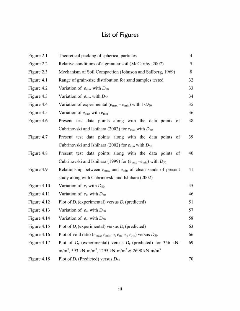
List of Figures

Figure 2.1 Theoretical packing of spherical particles 4

Figure 2.2 Relative conditions of a granular soil (McCarthy, 2007) 5

Figure 2.3 Mechanism of Soil Compaction (Johnson and Sallberg, 1969) 8

Figure 4.1 Range of grain-size distribution for sand samples tested 32

Figure 4.2 Variation of emax with D50 33

Figure 4.3 Variation of emin with D50 34

Figure 4.4 Variation of experimental (emax – emin) with 1/D50 35

Figure 4.5 Variation of emax with emin 36

Figure 4.6 Present test data points along with the data points of

Cubrinovski and Ishihara (2002) for emax with D50

38

Figure 4.7 Present test data points along with the data points of

Cubrinovski and Ishihara (2002) for emin with D50

39

Figure 4.8 Present test data points along with the data points of

Cubrinovski and Ishihara (1999) for (emax –emin) with D50

40

Figure 4.9 Relationship between emax and emin of clean sands of present

study along with Cubrinovski and Ishihara (2002)

41

Figure 4.10 Variation of es with D50 45

Figure 4.11 Variation of em with D50 46

Figure 4.12 Plot of Dr (experimental) versus Dr (predicted) 51

Figure 4.13 Variation of ers with D50 57

Figure 4.14 Variation of em with D50 58

Figure 4.15 Plot of Dr (experimental) versus Dr (predicted) 63

Figure 4.16 Plot of void ratio (emax, emin, es em, ers erm) versus D50 66

Figure 4.17 Plot of Dr (experimental) versus Dr (predicted) for 356 kN-

m/m3, 593 kN-m/m3, 1295 kN-m/m3 & 2698 kN-m/m3

69

Figure 4.18 Plot of Dr (Predicted) versus D50 70

iv

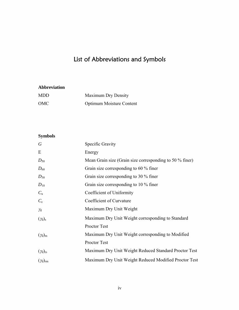
List of Abbreviations and Symbols

Abbreviation

MDD Maximum Dry Density

OMC Optimum Moisture Content

Symbols

G

E

Specific Gravity

Energy

D50

D60

D30

D10

Mean Grain size (Grain size corresponding to 50 % finer)

Grain size corresponding to 60 % finer

Grain size corresponding to 30 % finer

Grain size corresponding to 10 % finer

Cu Coefficient of Uniformity

Cc Coefficient of Curvature

γd Maximum Dry Unit Weight

(γd)s Maximum Dry Unit Weight corresponding to Standard

Proctor Test

(γd)m Maximum Dry Unit Weight corresponding to Modified

Proctor Test

(γd)rs Maximum Dry Unit Weight Reduced Standard Proctor Test

(γd)rm Maximum Dry Unit Weight Reduced Modified Proctor Test

v

e

emax

emin

es

em

ers

erm

Void Ratio

Maximum Void Ratio

Minimum Void Ratio

Void Ratio corresponding to Standard Proctor Test

Void Ratio corresponding to Modified Proctor Test

Void Ratio corresponding to Reduced Standard Proctor Test

Void Ratio corresponding to Reduced Modified Proctor Test

Dr

(Dr)s

(Dr)m

(Dr)rs

(Dr)rm

Rc

Relative Density

Relative Density corresponding to Standard Proctor Test

Relative Density corresponding to Modified Proctor Test

Relative Density corresponding to Reduced Standard Proctor

Test

Relative Density corresponding to Reduced Modified Proctor

Test

Relative Compaction

0

CHAPTER 1

INTRODUCTION

1

INTROUCTION

1.1 BACKGROUND

Compaction is a process of mechanical soil improvement; and is by far the most commonly used

method of soil stabilization. Compaction is used to alter the engineering properties of a soil for a

specific application, such as supporting a pavement section, building foundation, or bridge

abutment etc. Density measurements are used in the field indirectly to gauge the effectiveness of

the compaction process with an aim of improving soil behavior for the intended application.

Compaction test is one of the tests that should be carried out before the other works started. The

strength of soils is mostly dependent on types of soils, its density and its moisture content which

can be obtained from compaction tests. The effectiveness of a compaction depends on few

factors out of which compactive effort (types of equipment, weight of equipment, vibration,

number of passes) is one of the factors that affects the compaction qualitatively. The main

objective of the study is to find the effects of different compaction energy on the soil compaction

parameters. Field compaction of sands usually involves different equipments with the

compaction energy varying significantly. By comparing the different compaction energy, the

standard Proctor and modified Proctor tests had been used to show the comparisons. Several

activities have been identified to achieve the objectives, i.e., literature review, conducting tests in

the laboratory, and analysing the results obtained from the laboratory tests. The Maximum Dry

Density of soils increases when there is an increase in the compaction energy but the Optimum

Moisture Content value decreases with increasing compaction energy/efforts. For cohesionless

soils containing very little or no fines the water content has influence on the compacted density.

At low water contents and particularly under a low compactive effort, density may decrease

compared to that produced by the same compactive effort for air dried or oven dried soil. This

decrease in density is due to the capillary tension which is not fully counteracted by compactive

effort and which holds the particle in a loose state resisting compaction. Density reaches

maximum when a cohesionless soil is fully saturated. Again, this maximum density may not be

very much higher than that corresponding to the air or oven dried condition. Attainment of

maximum density at full saturation should not be considered as due to the lubricating action of

water but rather due to the reduction of effective pressure between soil particles by hydrostatic

2

pressure. Hence the compaction characteristics (maximum dry unit weight and optimum

moisture content) need to be obtained at different compaction energies. For cohesionless soil like

sand it is better to express compaction behavior in terms of relative density. The relative density

(Dr) of granular soils may be a better indicator for end-product compaction specifications than

relative compaction. Thus knowledge of relative densities of sands at different compaction

energies assumes great importance from the viewpoint of practical significance. Limit density

values of sands should be regarded as important properties as the coefficient of uniformity (Cu),

coefficient of curvature (Cc), mean particle size (D50), and particle shape, among others, when

providing a thorough description of sand. Density (or void ratio) limits help to more completely

describe the material under consideration and are required when evaluating relative density of in-

place soils. The maximum and minimum (limit) density values represent the theoretical upper

and lower density boundaries for a given soil specimen (Holtz 1973). The maximum and

minimum density values are among some of the most important properties to include when

describing a sand specimen. Relative densities, maximum and minimum void ratio values of

sand are greatly affected by particle shapes, sizes and their packing.

0

CHAPTER 2

LITERATURE REVIEW

3

LITERATURE REVIEW

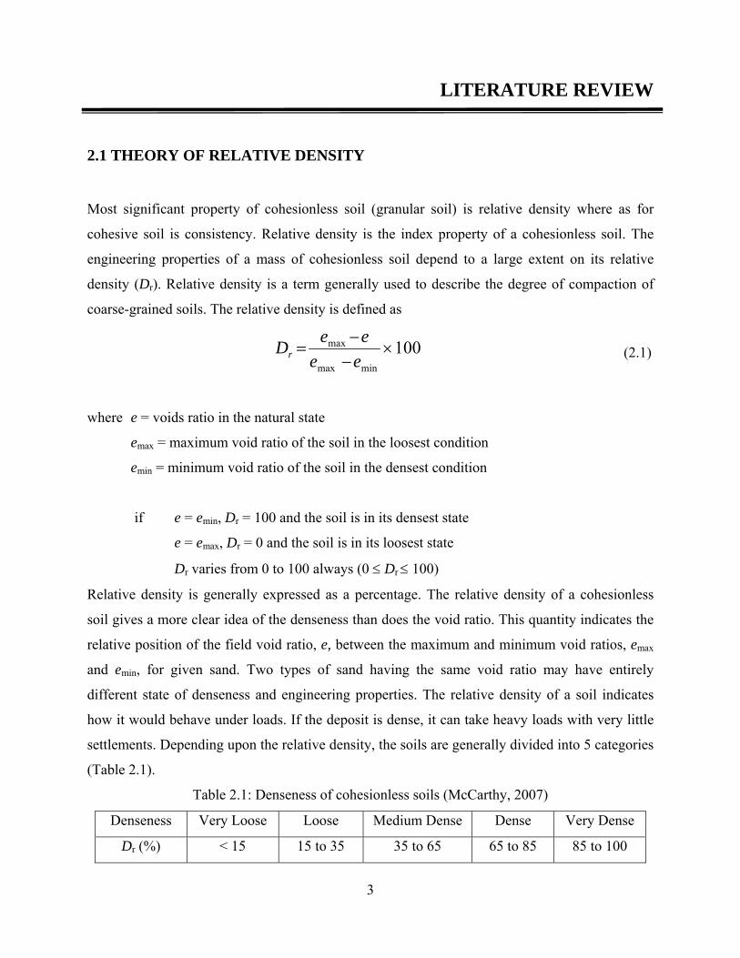
2.1 THEORY OF RELATIVE DENSITY

Most significant property of cohesionless soil (granular soil) is relative density where as for

cohesive soil is consistency. Relative density is the index property of a cohesionless soil. The

engineering properties of a mass of cohesionless soil depend to a large extent on its relative

density (Dr). Relative density is a term generally used to describe the degree of compaction of

coarse-grained soils. The relative density is defined as

100

minmax

max ×−−

=eeeeDr

(2.1)

where e = voids ratio in the natural state

emax = maximum void ratio of the soil in the loosest condition

emin = minimum void ratio of the soil in the densest condition

if e = emin, Dr = 100 and the soil is in its densest state

e = emax, Dr = 0 and the soil is in its loosest state

Dr varies from 0 to 100 always (0 ≤ Dr ≤ 100)

Relative density is generally expressed as a percentage. The relative density of a cohesionless

soil gives a more clear idea of the denseness than does the void ratio. This quantity indicates the

relative position of the field void ratio, e, between the maximum and minimum void ratios, emax

and emin, for given sand. Two types of sand having the same void ratio may have entirely

different state of denseness and engineering properties. The relative density of a soil indicates

how it would behave under loads. If the deposit is dense, it can take heavy loads with very little

settlements. Depending upon the relative density, the soils are generally divided into 5 categories

(Table 2.1).

Table 2.1: Denseness of cohesionless soils (McCarthy, 2007)

Denseness Very Loose Loose Medium Dense Dense Very Dense

Dr (%) < 15 15 to 35 35 to 65 65 to 85 85 to 100

4

At any given void ratio the strength and compressibility characteristics of grannular soil is almost

independent of the degree of saturation. The density of granular soil varies with its shape, size of

the soil grains, gradation and the manner in which soil is compacted. If all the soil grains are

assumed as spheres of uniform size then theoretically packed one are shown as in the Figure 2.1.

Loosest State Densest State

(Soil grains are one above another) (Soil grains are in between two)

Cubical Face-centered cubical or (Pyramidal)

Close-packed hexagonal (Tetrahedral)

Figure 2.1 Theoretical packing of spherical particles

The soil corresponding to higher void ratio is in the loosest state and lower void ratio is in the

densest state. If the soil grains are not uniform then the smaller grains fill in the space between

the bigger ones and void ratio of such soils is reduced to e = 0.25. In the dense state if the soil

grains are angular then they tend to form loosest structures than rounded grains because their

sharp edges and points hold the grains further apart. But, if the soil mass with angular grains, is

compacted by vibration then it forms a dense structure. A static load alone will not change the

density of the grains significantly, but if it is accompanied by vibration there will be considerable

increase in density. The water content in the void may act as lubricant to certain extent for

increase in the density under vibration. Since the change in void ratio would change the density

5

and this in turn will change the strength characteristics of granular soils. Void ratio or unit

weight of the soil can be used to compare the strength characteristics of granular soils of the

same origin. The properties and characteristic behavior patterns of granular materials are most

often related to the relative density. So, the relative density is used to indicate the strength

characteristics in qualitative manner. But, there are sudden practical difficulties in determining

the void ratio. One of the problem involved lies in measuring the solid volume. So, in order to

overcome this difficulty the relative density is expressed in terms of the dry unit weights

associated with the various void ratios. They depend on various factors like soil type

(mineralogy), particle grading, and angularity etc. In Figure 2.2 soils are in the densest, natural

and loosest state. As it if difficult to measure the void ratio directly, it is convenient to express

the void ratio in terms of dry density.

e min

Solid

Intermediate condition Loosest conditionDensest condition

Air

Solid

Air

Solid

Air

V V VS S S

VV

V

vv

v

Void ratio = e0Void ratio = e maxVoid ratio =

Figure 2.2 Relative conditions of a granular soil (McCarthy, 2007)

From the definitions we have,

1−=

d

wsGe

γ

γ

(2.2)

1

min

max −=d

wsGe

γ

γ

(2.3)

6

1

max

min −=d

wsGe

γ

γ

(2.4)

and hence

)(

)(

11

11

minmax

minmax

maxmin

min

ddd

ddd

dd

ddrD

γγγ

γγγ

γγ

γγ−

−=

−

−

=

(2.5)

where dγ = dry unit weight of soil in natural state

maxdγ = maximum dry unit weight of the soil corresponding to densest state

mindγ = minimum dry unit weight of the soil corresponding to loosest state

The expression for relative density can also be written in terms of porosity as,

)1()(

)1()(

minmax

minmax

ηηη

ηηη

−−

−−=rD

(2.6)

where η = porosity of soil in natural state

maxη = maximum porosity at loosest state

minη = minimum porosity at densest state

Several investigators have attempted to correlate relative density with the angle of internal

friction of soil. Meyerhof (1956) suggested relationship between angle of internal friction (Φ)

and relative density.

rD15.0250 +=φ (Granular soils or sands with more than 5 % silt) (2.7)

rD15.0300 +=φ (Granular soils or sands with less than 5 % silt) (2.8)

7

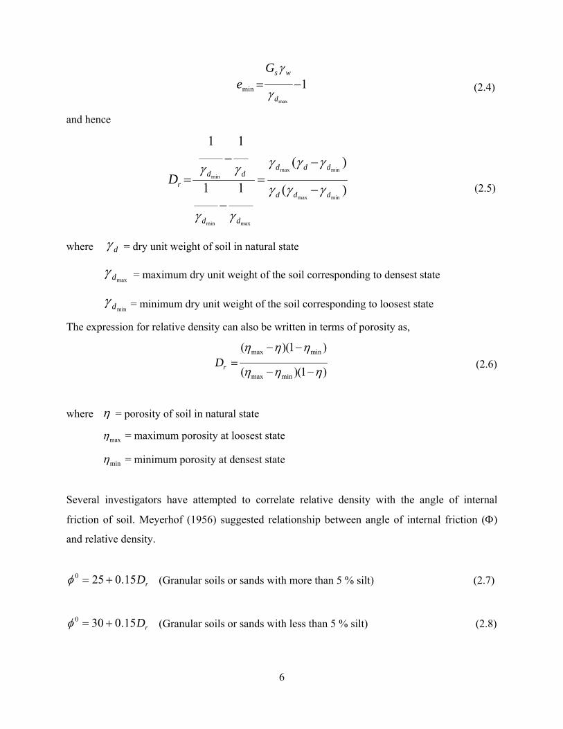
Another term occasionally used in regard to the degree of compaction of coarse-grained soils is

relative compaction (Rc) (Das, 2008) which is defined as

maxd

d

cRγ

γ=

(2.9)

Rc in terms of relative density,

)1(1 0

0

RD

RR

rc −−= (2.10)

where Rc and Dr are not in per cent and max

min

0d

d

Rγ

γ=

Lee and Singh (1971) reviewed 47 different soils and gave the approximate relation between

relative compaction and relative density as follows:

rc DR 2.080 += (2.11)

where Rc and Dr are in per cent

Rc = 80% (minimum) corresponding to Dr =0

Dr =0 represents loosest state

Rc = 100% represents dense state

2.2 THEORY OF COMPACTION

Compaction is the densification of a soil by mechanical means. It is determined by measuring the

in-place density of the soil and comparing it to the results of a laboratory compaction test. Soil

compaction occurs when soil particles are pressed together, reducing pore space between them.

Heavily compacted soils contain few large pores and have a reduced rate of both water

infiltration and drainage from the compacted layer. This occurs because large pores are most

effective in moving water through the soil when it is saturated. In addition, the exchange of gases

slows down in compacted soils, causing an increase in the likelihood of aeration-related

problems (Holtz, 1981). Soil compaction changes pore space size, distribution, and soil strength.

8

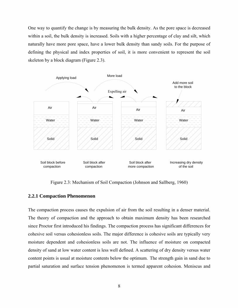
One way to quantify the change is by measuring the bulk density. As the pore space is decreased

within a soil, the bulk density is increased. Soils with a higher percentage of clay and silt, which

naturally have more pore space, have a lower bulk density than sandy soils. For the purpose of

defining the physical and index properties of soil, it is more convenient to represent the soil

skeleton by a block diagram (Figure 2.3).

Soil block before compaction

Soil block after compaction

Soil block aftermore compaction

Increasing dry density of the soil

Add more soil to the block

Applying load More load

Expelling air

Water

Air

Solid

Water

Air

Water

Air

Water

Air

Solid Solid Solid

Figure 2.3: Mechanism of Soil Compaction (Johnson and Sallberg, 1960)

2.2.1 Compaction Phenomenon

The compaction process causes the expulsion of air from the soil resulting in a denser material.

The theory of compaction and the approach to obtain maximum density has been researched

since Proctor first introduced his findings. The compaction process has significant differences for

cohesive soil versus cohesionless soils. The major difference is cohesive soils are typically very

moisture dependent and cohesionless soils are not. The influence of moisture on compacted

density of sand at low water content is less well defined. A scattering of dry density versus water

content points is usual at moisture contents below the optimum. The strength gain in sand due to

partial saturation and surface tension phenomenon is termed apparent cohesion. Meniscus and

9

surface tension along with the apparent cohesion will disappear when the sand is fully saturated

or dries (McCarthy, 2007).

Proctor (1933) recognized that moisture content affects the compaction process. He believed that

the cause for a moisture-density curve “breaks over” at optimum moisture content was related to

capillarity, frictional forces. He also believed that the force of the compactive effort applied was

another factor to overcome the inter-particle friction of the particles. As the water content

increased from dry of optimum to wet of optimum, he believed that the water acted as a lubricant

between the soil particles. The addition of more water continued to aid the compaction process

until the water began replacing the air voids. At this point the compaction process was complete

and the addition of more compactive energy would not result in a denser soil.

Lambe (1969) studied the microstructure of clays and developed a theory based on

physicochemical properties. He found that compaction of a soil dry of optimum moisture content

results in a flocculated soil structure that has high shear strength and permeability. Compaction

of a soil wet of optimum moisture content results in a soil with a dispersed soil structure that has

low shear strength and permeability. While this information does not directly explain the shape

of the compaction curve, it does help explain the strength and volume characteristics of

compacted soils.

According to Winterkorn and Fang (1975), the compaction theories based on effective stresses,

explain the shape of the compaction curve better than the theories based on lubrication and

viscous water. The facts that soils are anisotropic and heterogeneous complicate the research

process and add validity to Terzaghi’s remarks about large-scale field tests.

Hilf (1956), as summarized by Winterkorn and Fang (1975), presented another theory about the

compaction phenomenon. The theory is based on pore water pressures in unsaturated soils. He

developed a curve based on void ratio and water-void ratio. The curve looks similar to a typical

moisture-density curve because the minimum void ratio is also the maximum density optimum

moisture content point on a moisture density curve. Capillary pressure and pore pressure explain

the shape of the curve. The menisci of the water in a drier soil have a high curvature and are

stronger than a wetter soil with flatter menisci. The decrease in density after optimum moisture

10

content was attributed to the trapping of air bubbles and a buildup of pore pressure lowering the

effectiveness of compaction. The buildup of negative pore pressure in the moisture films

surrounding the soil particles were assumed to be interconnected and resulted in an effective

compressive stress on the soil skeleton equal to the negative pressure. Subsequent research has

shown that capillary pressure may not act as an effective stress in unsaturated soils. An X factor

that varies from 0 to 100 with saturation relates how much the capillary pressure acts as an

effective stress. This X factor is very difficult to measure and therefore Hilf’s theory is still

controversial.

Hogentogler, summarized by Hausmann (1990), introduced the next major compaction theory.

He also thought that water was a lubricant in the compaction process. He described compaction

along the moisture density curve from dry to wet as a four-step process. First, the soil particles

become hydrated as water is absorbed. Second, the water begins to act as a lubricant helping to

rearrange the soil particles into a denser and denser state until optimum moisture content is

reached. Third, the addition of water causes the soil to swell because the soil now has excess

water. Finally, the soil approaches saturation as more water is added. His theory was disproven

when research showed that the compaction process does not result in complete saturation and

compaction wet of optimum moisture content will tend to parallel the zero-air voids curve rather

than intersect it.

2.2.2 Field compaction of cohesionless soils

The compaction process may be accomplished by rolling, tamping or vibration. The compaction

characteristics are first determined in the laboratory by various compaction tests. The main aim

of these tests is to arrive at a standard which may serve as a guide and a basis of comparison for

field compaction (Johnson and Sallberg, 1960). Vibratory compaction with smooth drum

machines is especially suitable and economical on sand and gravel. High densities can be

achieved in few passes with the lift thickness determined by the size of the compactor (D’

Appolonia, et al., 1969). Free-draining sand and gravel that contains less than 10% fines are

easily compacted, especially when water saturated. When high density is required and the lifts

are thick, water should be added. This water will drain out of the lift during the compaction

process. If the sand and gravel contains more than 10% fines, the soil is no longer free draining

11

and may become elastic when the water content is high. For this type of soil, there will be

optimum moisture content at which maximum density can be reached. Drying of the wet soil

may be necessary to reach the optimum moisture content. On poorly graded sand and gravel, it is

difficult to achieve high density close to the surface of the fill. There is low shear strength in

poorly graded soils and the top layer tends to rise up behind the drum. This is not a problem

when multiple lifts are being compacted. The previous top layer will be compacted when the

next layer is rolled. However, the difficulty of compacting the surface should be kept in mind

when testing for density.

2.3 Previous Work on Laboratory Density Test and Theoretical Analysis

The experimental and analytical studies carried out by various investigators on relative density &

compaction behaviour of sand were reviewed and briefly presented in this chapter.

White and Walton (1937) studied on particle packing and particle shape. Relative densities,

maximum and minimum void ratio values of sand are greatly affected by particle shapes, sizes

and their packing. Spherical particles of equal size theoretically may be packed in five different

ways, e.g. (1) cubical with a theoretical void space of 47.64%, (2) single-staggered or cubical-

tetrahedral with a theoretical void space of 39.55%, (3) double-staggered with a theoretical void

space of 30.20%, (4) pyramidal, and (5) tetrahedral; the void spaces in the latter two are

identical, 25.95%. Secondary, ternary, quaternary, and quinary spheres each set smaller than its

predecessor, may be fitted into the voids in this last type of packing and the voids reduced

theoretically to 14.9%. The use of very fine filler in the remaining voids will then reduce the

voids theoretically to 3.9%. The use of particles of elliptical shape does not appear to reduce the

porosity, but cylindrical-shaped particles, if properly arranged, would reduce the porosity. The

practical application of these theoretical methods of packing was studied.

Burmister (1948) offered an analogy regarding limit densities for sands. Limit density values of

sands should be regarded as important as such properties as the coefficient of uniformity (Cu),

coefficient of curvature (Cc), the mean particle size (D50), and particle shape, among others,

when providing a thorough description of sand. Density (or void ratio) limits help to more

12

completely describe the material under consideration and are required when evaluating relative

density of in-place soils.

Lee and Suedkamp (1972) studied on the compaction of granular soils and found compaction

curve can be irregular if compaction tests are carried out using a larger number of test points and

range of moisture contents extending towards zero. Exact form of the curve depends on the type

of the material. They found four types of compaction curve such as bell shaped (30 < wL< 70),

one & one-half peak (wL< 30), double peak (wL< 30 or wL< 70 ) and odd shaped (wL> 70).

Selig and Ladd (1973) presented evaluation of relative density measurements and applications.

The source and type of errors in relative density are assessed. Based on reported values of

maximum, minimum, and density errors, expected errors in relative density are determined.

These values may be used as a basis for setting confidence limits on the results of studies

involving relative density. Engineering applications of the relative density parameter are

discussed, and alternatives to relative density are given. Factors influencing the maximum and

minimum densities used in calculating relative density are summarized. Experience in correlating

relative density to blow count and strength of cohesionless materials is reviewed. Finally, based

on all of the information gathered in the symposium, a series of recommendations are given for

modifications to the ASTM test procedures and for needed new procedures.

Townsend (1973) presented comparisons of vibrated density and standard compaction tests on

sands with varying amounts of fines. The effects of gradation, percentage and plasticity of fines,

and moisture on vibratory and impact compaction of granular soils were investigated by adding

measured percentages of low plasticity (ML) and medium plasticity (CL) fines to a poorly

graded (SP) and nearly well graded (SW-SP) sand. Results indicated that more fines can be

added to uniform sand and that uniform sand densities by vibration more effectively than well

graded sand. The same densities are produced by impact and vibratory compaction at higher

percentage of fines added to the well graded sand compared to the percent fines added to the

uniform sand. Moisture and plasticity are interrelated factors which greatly affect compaction.

Saturation facilitated vibratory compaction of low plasticity mixtures; however, for more plastic

mixtures, adhesion of the fines to the sand grains restricted vibratory densification. Current

compaction test selection criteria, which ignore plasticity and moisture effects by comparing

13

vibratory densities of oven-dry materials with those, determined by standard compaction, can

lead to the untenable conclusion that vibratory compaction should be used for sands containing

in excess of 20 percent fines.

Holubec and D'Appolonia (1973) studied the effect of particle shape on the engineering

properties of granular soils. The use of relative density correlations based on an average sand to

predict soil behavior without considering the particle shape can result in poor or misleading

predictions. Experimental data indicated that the particle shape has a pronounced effect on all

engineering properties. Angularity of the particles increases the maximum void ratio, strength,

and deformability of cohesionless soils. Variations in engineering properties due to particle

shape can be as large as variations associated with large differences in relative density.

Penetration tests in small containers with small rods suggest that the Standard Penetration Test is

influenced by both the angularity and density of cohesionless soils.

Youd (1973) studied the factors controlling maximum and minimum densities of sands.

Maximum and minimum density tests, conducted on a variety of clean sands, found that the

minimum and maximum void-ratio limits are controlled primarily by particle shape, particle size

range, and variances in the gradational-curve shape, and that the effect of particle size is

negligible. Curves were developed for estimating minimum and maximum void ratios from

gradational and particle-shape parameters. Estimates for several natural and commercially

graded sands agree well with minimum and maximum void ratios measured in the laboratory.

Minimum densities (maximum void ratios) were determined by the standard American Society

for Testing and Materials (ASTM), minimum density test method (Test for Relative Density of

Cohesionless Soils (D 2049-69)), except that smaller moulds were used. Maximum densities

(minimum void ratios) were determined by repeated straining in simple shear, a method which

has been shown to give greater densities than standard vibratory methods.

Dickin (1973) studied the influence of grain shape and size upon the limiting porosities of sands.

The state of packing of a mass of sand grains is described by its relative porosity which defines

the packing relative to maximum and minimum porosities of the material. These limiting

porosities depend in turn upon the physical characteristics of the grains themselves. The

influence of grain shape and size upon the limiting porosities of quartz sands and glass ballotini

14

was studied. The maximum porosities were determined by deposition of the sample through

water as suggested by Kolbuszewski (1948) while minimum porosities were obtained by

vibration under water. Shape parameters for the sands were determined from a correlation

between the time of flow of a 0.5-kg specimen and the sphericity measured by examination of

individual grains. Both maximum and minimum porosities decreased with increasing sphericity

while tests on glass ballotini indicated that the effect of grain size was negligible. The porosity

interval was approximately 12.5 percent for all the sands and 11 percent for spherical ballotini.

Mixtures of sand and ballotini gave reasonable agreement with the trend shown by the separate

materials.

Johnston (1973) presented laboratory studies of maximum and minimum dry densities of

cohesionless soils. Some of the differences in results of tests for the maximum and minimum dry

densities of cohesionless soils were examined. He investigated the reproducibility of results of

maximum and minimum densities for two types of sands by a comparative test program and

suggested an empirical correlation for the uniformity coefficient versus maximum and minimum

densities. He gave comparison between the Providence Vibrated Density method and the

vibratory table method. The results shown that one of the important variables in determining the

maximum density of cohesionless soils using the vibratory table method was the amplitude of the

vibrating mould.

Walter et al. (1982) determined the maximum void ratio of uniform cohesionless soils. A testing

program was conducted to evaluate several methods of determining the maximum void ratio of

cohesionless soils. Preliminary test results indicated that a new procedure called the tube method

was consistent in attaining reliable maximum void ratios. In performing the tube method, a long

narrow tube or cylinder opened at both ends was placed upright in a mold of known volume. A

quantity of dry sand sufficient to fill the mold was placed in the tube and then the tube was

slowly extracted to allow sand to trickle into the mold until the mold overflows. The sand was

then screeded level with the top of the mould and the void ratio was calculated from measured

masses and volumes and the specific gravity of the sand. To evaluate various methods of

determining maximum void ratios, a test series was carried out by using eight different test

procedures on four sands. Statistical analyses of the data indicated that the tube method yielded

higher values of maximum void ratio than did the other procedures. In addition, a testing

15

program involving nine inexperienced operators demonstrated that by using the tube method an

individual operator was able to reproduce results consistently and the operators were able to

replicate one another's results well within limits mandated by practical applications.

Aberg (1992) presented void ratio of non cohesive soils and similar materials. A new approach

was presented to the topic of numerical description of void characteristics of noncohesive soils

and similar granular materials. Based upon a simple stochastic model of the void structure and

void sizes, theoretical equations were derived by means of which the void ratio of a soil can be

calculated from its grain-size distribution. The calculations also give information about type of

grain structure and the grain size that separates fixed grains and possible loose grains were

determined. The equations also considered the grain shape, degree of densification, and size of

compaction container. Results of numerous laboratory compaction tests on uniform to broadly

graded sand, gravel, and crushed-rock materials confirm the general forms of the derived

equations, were the basis for evaluation of certain parameters.

Aberg (1996) investigated grain-size distribution for smallest possible void ratio. The theoretical

equations for void ratio as a function of grain size distribution were used to find the grain size

distribution that give the smallest possible void ratio for highly densified, cohesion less soils and

similar materials. Both numerical and analytical methods were used. He also studied the void

sizes in granular soils. The stochastic model was used to find the distribution of void volume as a

function of void size (void-chord length).

Lade et al. (1998) studied the effects of non-plastic fines on minimum and maximum void ratios

of sand. The behavior of sand was affected by the content of non-plastic fine particles. They have

studied the effect of degree of fines content on the minimum and maximum void ratios. A review

was presented of previous theoretical and experimental studies of minimum and maximum void

ratios of single spherical grains, packings of spheres of several discrete sizes, as well as optimum

grain-size ratios to produce maximum densities. A systematic experimental study was performed

on the variation of minimum and maximum void ratios to signify the contents of fines for sands

with smoothly varying particle size curves and a large variety of size distributions. It was shown

that the fines content plays an important role in determining the sand structure and the

consequent minimum and maximum void ratios.

16

Masih (2000) developed a mathematical formula to get desired soil density. He used statistical

parameters of the soil grains distribution to predict the soil maximum dry density and then

applied the fine biasness coefficient to predict the new density of the soil after mixing any

amount of fine particles with the original soil. Lab testing results were compared with the results

of the prediction. They were found to be in total agreement, and the margin of error was found to

be quite low.

Barton et al. (2001) measured the effect of mixed grading on the maximum dry density of sands.

During cut and fill operations, compaction using sands from different sources may be carried out.

The resulting mixed sand will have different compaction characteristics than those of the parent

sands. An increase in dry density will result as the grading moves towards more ideal

characteristics for dense packing. Laboratory compaction tests using pluviation and the vibrating

hammer method have been carried out to measure this increase in dry density. The resulting

value was generally significantly greater than the result predicted by taking the mean value of

dry density given by the parent sands.

Cubrinovski and Ishihara (2002) studied the maximum and minimum void ratios characteristics

of sands. Characteristics of the maximum and minimum void ratios of sands and their possible

use for material characterization have been investigated in this study. Data of over 300 natural

sandy soils including clean sands, sands with fines and sands containing small amount of clay-

size particles have been used to examine the influence of fines, grain-size composition and

particle shape on emax, emin and void ratio range (emax - emin). A set of empirical correlations were

presented which clearly demonstrate the link between these void ratios and material properties of

sands. The key advantage of (emax - emin) over conventional material parameters such as Fc and

D50 is that (emax - emin) was indicative of the overall grain-size composition and particle

characteristics of a given sand and found the combined influence of relevant material factors.

The void ratio range indicated a general basis for comparative evaluation of material properties

over the entire range of cohesionless soils. Three distinct linear correlations were found to exist

between emax and emin for clean sands, sands with 5-15% fines and sands with 15-30% fines

respectively, thus illustrated that the standard JGS procedures for minimum and maximum

17

densities of sands can provide reasonably consistent emax and emin values for sands with fines

content of up to 30%.

Omar et al. (2003) investigated the compaction characteristics of granular soils in United Arab

Emirates. A study was undertaken to assess the compaction characteristics of such soils and to

develop the governing predictive equations. For the purposes of this study, 311 soil samples were

collected from various locations in the United Arab Emirates and tested for various including

grain-size distribution, liquid limit, plasticity index, specific gravity of soil solids, maximum dry

density of compaction, and optimum moisture content following ASTM D 1557-91 standard

procedure C. A new set of 43 soil samples were collected and their compaction results were used

to test the validity of predictive model. The range of variables for these soils were as follows:

percent retained on US sieve #4 (R#4): 0–68; Percent passing US sieve #200 (P#200): 1–26;

Liquid limit: 0–56; Plasticity index: 0–28; Specific gravity of soil solids: 2.55–2.8. Based on the

compaction tests results, multiple regression analyses were conducted to develop mathematical

models and nomographic solutions to predict the compaction properties of soils. The results

indicated that the nomographs could predict well the maximum dry density within ±5%

confidence interval and the optimum moisture content within ±3%.

Itabashi et al. (2003) studied the grain shape and packing property of unified coarse granular

materials. Particle shape analysis and random packing experiences were carried out used by

unified stainless ball and five natural granular materials which were produced under different

natural environments. They found that three particle shape parameters (form unevenness FU,

order number Mi and fractal dimension FD) of six granular materials much differ from each

other, and these were able to evaluate the difference of ultimate porosity.

Hatanaka and Feng (2006) estimated relative density of sandy soils from SPT-N value. The

applicability of three previous empirical correlations proposed for estimating relative density of

sandy soils based on the SPT N-value, effective overburden stress and soil gradation

characteristics was investigated using a data base of relative density obtained from high quality

undisturbed samples of fine to medium sand with Fc ≤ 20％, D50 ≤ 1.0 mm and Dmax ≤ 4.75 mm.

All undisturbed samples were recovered by in-situ freezing method. The relative density

estimated by Meyerhof′s method (1957) was in the range of ＋15％～－45％ of the measured

18

values. Meyerhof′s method (1957) was modified by Tokimatsu and Yoshimi (1983) by

considering the effect of fines content on the SPT N-value. The relative density estimated by

Tokimatsu and Yoshimi′s method (1983) was in the range of ＋25％～－20％ of the measured

values. The underestimation of relative density of Meyerhof′s method (1957) was modified. On

the contrary, the overestimation of relative density was more significant than Meyerhof′s

method. The relative density estimated by the method proposed by Kokusho et al. (1983) was in

the range of ＋20％ to －35％ of the measured values even for dense sand with a relative

density larger than 60％. Meyerhof′s method (1957) and the method proposed by Kokusho et al.

(1983) have a common disadvantage that they will extremely underestimate the relative density

of fine to medium sand for SPT N-value lower than about 8. A simple empirical correlation was

proposed to estimate the relative density of fine to medium sand based on the normalized SPT N-

value, N1. The relative density estimated by the proposed method was in the range of ＋ 15％ to

－30％ of the measured values for N1 in the range between 0 and 50. As a whole, the proposed

method was less in errors for estimating relative density compared with those estimated by

Meyerhof′s method (1957) and the method proposed by Kokusho et al. (1983). Based on a data

base of undisturbed samples with data of fines content obtained from the SPT spoon samples, the

method proposed was again compared with the three previous methods. The relative density

estimated by the proposed method based on the above data base is in the range of ＋15％ to

－10％ of the measured values. Among four methods, as a whole, the proposed method found to

be the least errors in estimation of relative density. The proposed method was also modified by

taking into account of the effect of fines content of SPT samples. The relative density estimated

by the modified method based on the fines content is almost in the range of ＋10％ to － 10％

of the measured values. Two empirical correlations proposed were less in errors of estimating

relative density compared with three previous methods. The range of relative density estimated

was consistent with the range of the measured values (40％ to 90％). The empirical correlations

proposed in the study should be applied to fine to medium sand with Fc ≤ 20％, D50 ≤ 1.0 mm

and Dmax ≤ 4.75 mm.

Cho et al. (2006) studied the particle shape effects on packing density, stiffness and strength for

natural and crushed sands. The experimental data and results from published studies were

19

gathered into two databases to explore the effects of particle shape on packing density and on the

small-to-large strain mechanical properties of sandy soils. In agreement with previous studies,

these data confirmed that increase in angularity or eccentricity produces an increase in emax and

emin. Therefore, particle shape emerged as a significant soil index property that needs to be

properly characterized and documented, particularly in clean sands and gravels.

Muszynski (2006) determined the maximum and minimum densities of poorly graded sands

using a simplified method. The simplified method was easy to perform, requires less sample

volume, and was faster than the conventional methods for determining these properties. Results

of this study indicated that the simplified method gives limit density values comparable to those

obtained using conventional methods for clean poorly graded fine to medium sands. Limitations

of the simplified method were also discussed.

Sinha and Wang (2008) developed Artificial Neural Network (ANN) prediction models for soil

compaction and permeability. The ANN prediction models were developed from the results of

classification, compaction and permeability tests, and statistical analyses. The test soils were

prepared from four soil components, namely, bentonite, limestone dust, sand and gravel. These

four components were blended in different proportions to form 55 different mixes. The standard

Proctor compaction tests were adopted, and both the falling and constant head test methods were

used in the permeability tests. The permeability, MDD and optimum moisture content (OMC)

data were trained with the soil’s classification properties by using an available ANN software

package. Three sets of ANN prediction models were developed, one each for the MDD, OMC

and permeability (PMC). A combined ANN model was also developed to predict the values of

MDD, OMC, and PMC. A comparison with the test data indicate that predictions within 95%

confidence interval can be obtained from the ANN models developed.

Abdel-Rahman (2008) predicted the compaction of cohesionless soils using ANN. An artificial

neural network (ANN) model was developed to predict the two main compaction parameters: the

maximum dry unit weight (γd)max and the optimum moisture content (womc). The study was

performed based on the results of modified Proctor tests (ASTM D 1557). Based on the ANN

model, empirical equations were developed to predict the compaction characteristics of graded

cohesionless soils. The predicted values using the ANN model and the empirical equations were

20

compared with a set of laboratory measurements. A parametric study on the developed equations

was performed to present the control parameters that set the values of (γd)max and womc.

Gunaydın (2008) estimated the soil compaction parameters by using statistical analyses and

artificial neural networks. The data collected from the dams in some areas of Nigde (Turkey)

were used for the estimation of soil compaction parameters. Regression analysis and artificial

neural network estimation indicated strong correlations (r 2 = 0.70–0.95) between the compaction

parameters and soil classification properties. It has been shown that the correlation equations

obtained as a result of regression analyses are in satisfactory agreement with the test results.

21

2.4 MOTIVATION & OBJECTIVE OF PRESENT RESEARCH WORK

From the review of literature available, it is seen that enough work has been done on the void

ratio, angularity, grain shape, grain size and their packing arrangements of various types of soil.

Various testing methods for determining minimum and maximum voids ratio of sand, ANN

models and nomographs for predicting maximum dry density (MDD), optimum moisture content

(OMC) of soil have been presented by some investigators. However, accurate determination of

compaction parameters such as MDD and OMC of sand is difficult. In most specifications for

earthwork, the contractor is instructed to achieve a compacted field dry unit weight of 95 to 98%

of the maximum dry unit weight determined in the laboratory by either the standard or modified

Proctor test. For the compaction of granular soils, specifications are sometimes written in terms

of the required relative density. Empirical correlations have been made by earlier investigators in

predicting relative density of sandy soils from SPT test data in the field. It is reported in literature

that the maximum and minimum voids ratio decrease with increase in the mean grain size (D50).

Minimum and maximum voids ratios range (emax – emin) of sandy soils or soils with low fine

contents is a function of mean grain size (D50). From the available literature, it is learnt that the

correlation of relative density of granular soils have not been attempted in the laboratory with the

index property like grain size. Therefore, a relationship can be established in the laboratory with

emax, emin and mean grain size. Similarly the relative density at particular compactive effort can

be correlated with mean grain size of the granular soils.

The main objectives of present research work are as follows:

• Characterization of relative density of sand by establishing relationship between void

ratios with mean grain size (D50) with reference to different compaction energy.

• Prediction of maximum and minimum void ratio (emax, emin) from D50.

• Prediction of void ratios (e) from D50 corresponding particular energy level of compaction

• Prediction of Relative density of sand at the particular compaction energy level.

0

CHAPTER 3

EXPERIMENTAL PROGRAMME

22

EXPERIMENTAL PROGRAMME

The properties of soil which are indicative of the engineering properties are called index

properties. The tests which are required to determine the index properties are known as

classification tests. The soils are classified and identified based on the index properties. The main

index properties of sand are particle size and relative density.

3.1 TEST SPECIMENS

Natural sand samples were collected from 10 rivers of Orissa (Mahanadi, Kathojodi, Rushikulya,

Bramhni, Baitarani, Subarnarekha, Budhabalanga, Salandi, Daya, Koel). Total 55 samples were

used for the experimentation. Various tests such as specific gravity (G), grain size distribution

(D60, D50. D30, D10, Cu, Cc), and relative density (emax, emin, e) were conducted for determination

of basic physical properties.

3.2 TEST METHODOLOGY

3.2.1 Determination of specific gravity (G)

Specific gravity (G) of solid particles is the ratio of the mass of a given volume of solids to the

mass of an equal volume of gas-free distilled water at 40 C temperatures.

w

s

Gγ

γ=

(3.1)

where γs = unit weight of solid

γw = unit weight of water

The specific gravity of sand was determined in laboratory using a density bottle (as per IS:

2720 – Part III, 1980). The bottle of 250 ml capacity was cleaned and dried at a temperature of

1050 C to 1100 C and cooled. The weight of the bottle was taken. About 50 gm of oven dry

sample of sand was taken in the bottle and weighed. Distilled water was then added to cover the

23

sample and the sand was allowed to soak water for 30 minutes. Air entrapped in the sand was

expelled by gentle heating. More water was added to the bottle up to a mark and weighed. Then

the bottle was emptied, washed and refilled with distilled water up to that previous mark and

weighed. The specific gravity of sand was determined by the equation,

)()( 4312

12

MMMMMMG

−−−−

=

(3.2)

where M1 = mass of the empty bottle

M2 = mass of the empty bottle and dry sand

M3 = mass of the empty bottle, sand and water

M4 = mass of the bottle filled with water

3.2.2 Determination of grain size distribution

Particle size analysis or sieve analysis is a method of separation of sands into different fraction

based on the particle size. It expresses quantitatively the proportions, by mass of various sizes of

particles present in the sand. It is shown graphically on a particle size distribution curve. Oven

dry sand samples of 1000 gm were taken for sieve analysis. Sieves of size 4.75 mm, 2 mm, 1

mm, 600µ, 425µ, 300µ, 212µ, 150µ and75µ were used for sieving (as per IS: 2720 – Part IV,

1985). All samples were passed through 4.75 mm sieve and very little fines (< 5 %) were

retained in pan through 75µ sieve. Hence all samples were considered to be clean sands having

very little fines and no gravel fractions. By taking the weights of sand fraction retained on

various sieves, particle size distribution curve was plotted. The percentage finer (N) than a given

size has been plotted as ordinate (on natural scale) and the corresponding particle size as abscissa

(on log scale). The particle size distribution curve, also known as gradation curve represents the

distribution of particle of different sizes in the sand mass. The particle size distribution curve

also reveals whether the sand is well graded (particle of different sizes in good proportion) or

poorly graded (particle almost of same sizes). From this curve, mean grain size (D50), coefficient

of uniformity (Cu), and coefficient of curvature (Cc) were determined.

24

Mean grain size (D50) is the particle size corresponding to 50 % finer, which means 50 % of the

sand is finer than this size.

The uniformity of sand is expressed qualitatively by the term uniformity coefficient (Cu),

10

60

DDCu =

(3.3)

where D60 = particle size such that 60 % of the sand is finer than this size

D10 = effective size

= particle size such that 10 % of the sand is finer than this size

The larger the numerical value of Cu, the more is the range of particles. Sands with a value of Cu

less than 6 are poorly graded sand and value of Cu 6 or more, are well graded.

The general shape of particle size distribution curve is described by another coefficient known as

the coefficient of curvature (Cc) or the coefficient of gradation (Cg),

1060

230

DDDCc ×

=

(3.4)

where D30 = particle size corresponding to 30 % finer

D60 = particle size corresponding to 60 % finer

D10 = particle size corresponding to 10 % finer

For well graded sand, the value of Cc lies between 1 and 3 and for poorly graded sand the Cc

value is less than 1.

3.2.3 Determination of maximum void ratio (emax)

For determination of minimum dry density (maximum void ratio) of sand, oven dry sample of

sand was taken. The minimum dry density was found by pouring the dry sand in a mould using a

pouring device (as per IS: 2720 – Part XIV, 1983) and the spout of the pouring device was so

adjusted that the height of free fall was always 25 mm. A mould of volume 3000 cm3 was used

for the purpose. The weight and the volume of the sand deposited were found and the dry density

of the soil was determined as under,

25

VW

dmin

min=γ

(3.5)

where Wmin = weight of dry sand in the mould

V = volume of the mould

Then maximum void ratio can be determined by using the equation,

1min

max −⎟⎟⎠

⎞⎜⎜⎝

⎛=

d

wGeγγ

(3.6)

where G = specific gravity of sand

wγ = unit weight of water

mindγ = minimum dry unit weight of sand

3.2.4 Determination of minimum void ratio (emin)

The maximum dry density (minimum void ratio) was determined either by the dry method or the

wet method (as per IS: 2720 – Part XIV, 1983). In the dry method the mould was filled

thoroughly with mixed oven dry sand. A surcharge load was placed on the soil surface and the

mould was fixed to a vibrating table. The specimen was vibrated for 8 minutes. The weight of

the dry sand in the compacted state was found. The maximum dry density was given by

VW

dmax

max=γ

(3.7)

where Wmax = weight of dry soil

V = volume of the mould

Then minimum void ratio can be determined by using the equation,

1max

min −⎟⎟⎠

⎞⎜⎜⎝

⎛=

d

wGeγγ

(3.8)

where G = specific gravity of sand

wγ = unit weight of water

maxdγ = maximum dry unit weight of sand

26

The maximum dry density of sand was also determined in the saturated state. In this method, the

mould was filled with wet sand and water is added till a small quantity of free water accumulates

on the free surface of the sand. During and just after filling the mould, vibration was done for a

total of 6 minutes. Water appearing on the surface of sand was removed. A surcharge mass is

placed on the sand and the mould was vibrated again for 8 minutes. The weight (Wmax) of the

sand was determined after oven drying the sample. A mould volume of 3000 cm3was used for

both dry and wet method. For achieving the maximum dry density of sand out of 55 samples,

some samples were tested by above two methods i.e. dry method and wet method. However, the

results indicated that tests on dry condition gave maximum dry density. Therefore, the dry

method has been adopted for all the samples to get the minimum void ratio.

3.2.5 Determination of void ratio corresponding to maximum dry density (MDD)

Standard and modified Proctor compaction tests were used in the laboratory to determine the

maximum dry unit weight {γd(max–lab)} of soils to be used in the field. In most specification for

earth works, the contractor is instructed to achieve a compacted field dry unit weight of 95 to 98

% of the maximum dry unit weight determined in the laboratory by either the standard or

modified Proctor test (Arora, 2005). The maximum dry unit weight of compaction is used for

end-product specifications in terms of relative compaction (R) for construction work. Relative

compaction is defined as

100(%) )lab(max

)field( ×=−d

dcR

γγ

(3.9)

where γd(field) is the desired unit weight of compaction in the field.

For the compaction of granular soils, specifications are sometimes written in terms of the

required relative density (Dr) (Das, 2006). Holtz and Kovacs (1981) suggested that, for granular

soils with less than 12% fines (i.e., passing 0.075-mm sieve), relative density (Dr) may be a

better indicator for end-product compaction specifications than relative compaction. Relative

density (Dr) is defined as,

27

)(

)(

minmax

minmax

ddd

dddr

field

fieldDγγγ

γγγ

−

−= (3.10)

Relative density (Dr) in terms of void ratio,

100minmax

max ×−−

=ee

eeDr (3.11)

where emax, emin = maximum and minimum void ratios of the granular soil respectively

e = void ratio of the compacted soil.

The void ratios (e) obtained from the maximum dry unit weights of compaction for each type of

test (and, hence, compaction energy) were used to obtain the relative density of compaction. The

purpose of laboratory compaction testing is to find out how the sand may respond when

compacted on site. So the laboratory method, which best replicates the field compaction

equipment that is to be used on an earthworks job. Compaction tests at various energy levels

such as: Standard Proctor test, Modified Proctor test, Reduced Standard Proctor test, and

Reduced Modified Proctor tests have been conducted in the laboratory for the present work.

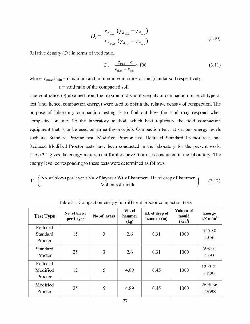
Table 3.1 gives the energy requirement for the above four tests conducted in the laboratory. The

energy level corresponding to these tests were determined as follows:

⎟⎠⎞

⎜⎝⎛ ×××

=mould of Volume

hammer of drop of Ht. hammer of Wt. layers of No. layer per blows of No.E

(3.12)

Table 3.1 Compaction energy for different proctor compaction tests

Test Type No. of blows per Layer

No .of layers Wt. of

hammer (kg)

Ht. of drop of hammer (m)

Volume of mould ( cm3)

Energy kN-m/m3

Reduced Standard Proctor

15 3 2.6 0.31 1000 355.80 ≅356

Standard Proctor

25 3 2.6 0.31 1000 593.01 ≅593

Reduced Modified Proctor

12 5 4.89 0.45 1000 1295.21 ≅1295

Modified Proctor

25 5 4.89 0.45 1000 2698.36 ≅2698

28

All the four tests as mentioned above are discussed below briefly.

Standard Proctor Compaction Test: (as per IS: 2720 – Part VII, 1980)

Sand was compacted into a mould in 3 equal layers, each layer receiving 25 numbers of blows of

a hammer weight 2.6 kg. The height of drop of hammer was 0.31m.The energy (compactive

effort) supplied in this test was 593 kN-m/m3.

Modified Proctor Compaction Test: (as per IS: 2720 – Part VIII, 1983)

Sand was compacted into a mould in 5 equal layers, each layer receiving 25 numbers of blows.

To provide the increased compactive effort (energy supplied = 2698 kN-m/m3) a heavier hammer

4.89 kg and a greater drop 0.45m height for the hammer were used.

Reduced Standard Proctor Compaction Test:

The procedure and equipment is essentially the same as that used for the Standard Proctor test.

However, each layer received 15 numbers of blows of a hammer/per each layer. The energy

(compactive effort) supplied in this test is 356 kN-m/m3.

Reduced Modified Proctor Compaction Test:

The procedure and equipment is essentially the same as that used for the Modified Proctor test.

Each layer of sand received 12 numbers of blows of a hammer/per each layer. The energy

(compactive effort) supplied in this test is 1295 kN-m/m3.

For determination of void ratio of sand corresponding to different energy levels an indirect

method was used. In this method corresponding to each energy level, maximum dry density

(MDD) was obtained from the compaction curve.

Then void ratio corresponding to that MDD was calculated by the following equation.

1−⎟⎟⎠

⎞⎜⎜⎝

⎛=

d

wGeγγ

(3.13)

where G = specific gravity of sand

wγ = unit weight of water

dγ = dry unit weight of sand corresponding to different energy levels

in Proctor test

29

3.2.6 Determination of relative density (Dr)

The relative density can be determined by the relation,

100

minmax

max

×−

−=

ee

eeDr

(3.14)

where

e = voids ratio calculated from laboratory proctor test,

emax = maximum voids ratio calculated from laboratory test

emin = minimum voids ratio calculated from laboratory test

The values of, emax, emin, e are mentioned as earlier in equations 3.6, 3.8 and 3.13 respectively.

The relative density corresponding to standard Proctor test, (Dr)s

100)(

minmax

max

×−

−=

ee

eeD

s

sr

(3.15)

where es = voids ratio calculated from MDD of standard Proctor test

The relative density corresponding to modified Proctor test, (Dr)m

100)(

minmax

max

×−

−=

ee

eeD

m

mr

(3.16)

where em = voids ratio calculated from MDD of modified Proctor test

The relative density corresponding to reduced standard Proctor test, (Dr)rs

100)(

minmax

max

×−

−=

ee

eeD

rs

rsr

(3.17)

where ers = voids ratio calculated from MDD of reduced standard Proctor test

The relative density corresponding to reduced modified Proctor test, (Dr)rm

100)(

minmax

max

×−

−=

ee

eeD

rm

rmr

(3.18)

where erm = voids ratio calculated from MDD of reduced modified Proctor test

0

CHAPTER 4

RESULTS AND DISCUSSION

30

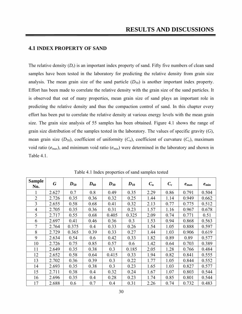
RESULTS AND DISCUSSIONS

4.1 INDEX PROPERTY OF SAND

The relative density (Dr) is an important index property of sand. Fifty five numbers of clean sand

samples have been tested in the laboratory for predicting the relative density from grain size

analysis. The mean grain size of the sand particle (D50) is another important index property.

Effort has been made to correlate the relative density with the grain size of the sand particles. It

is observed that out of many properties, mean grain size of sand plays an important role in

predicting the relative density and thus the compaction control of sand. In this chapter every

effort has been put to correlate the relative density at various energy levels with the mean grain

size. The grain size analysis of 55 samples has been obtained. Figure 4.1 shows the range of

grain size distribution of the samples tested in the laboratory. The values of specific gravity (G),

mean grain size (D50), coefficient of uniformity (Cu), coefficient of curvature (Cc), maximum

void ratio (emax), and minimum void ratio (emin) were determined in the laboratory and shown in

Table 4.1.

Table 4.1 Index properties of sand samples tested

Sample No. G D50 D60 D30 D10 Cu Cc emax emin

1 2.627 0.7 0.8 0.49 0.35 2.29 0.86 0.791 0.504 2 2.726 0.35 0.36 0.32 0.25 1.44 1.14 0.949 0.662 3 2.655 0.58 0.68 0.41 0.32 2.13 0.77 0.775 0.512 4 2.705 0.35 0.36 0.31 0.23 1.57 1.16 0.967 0.678 5 2.717 0.55 0.68 0.405 0.325 2.09 0.74 0.771 0.51 6 2.697 0.41 0.46 0.36 0.3 1.53 0.94 0.868 0.563 7 2.764 0.375 0.4 0.33 0.26 1.54 1.05 0.888 0.597 8 2.729 0.365 0.39 0.33 0.27 1.44 1.03 0.906 0.619 9 2.634 0.54 0.6 0.42 0.33 1.82 0.89 0.89 0.577 10 2.726 0.75 0.85 0.57 0.6 1.42 0.64 0.703 0.389 11 2.649 0.35 0.38 0.3 0.185 2.05 1.28 0.766 0.484 12 2.652 0.58 0.64 0.415 0.33 1.94 0.82 0.841 0.555 13 2.702 0.36 0.39 0.3 0.22 1.77 1.05 0.844 0.552 14 2.693 0.35 0.38 0.3 0.23 1.65 1.03 0.827 0.577 15 2.711 0.38 0.4 0.32 0.24 1.67 1.07 0.803 0.544 16 2.696 0.35 0.4 0.28 0.23 1.74 0.85 0.801 0.544 17 2.688 0.6 0.7 0.4 0.31 2.26 0.74 0.732 0.483

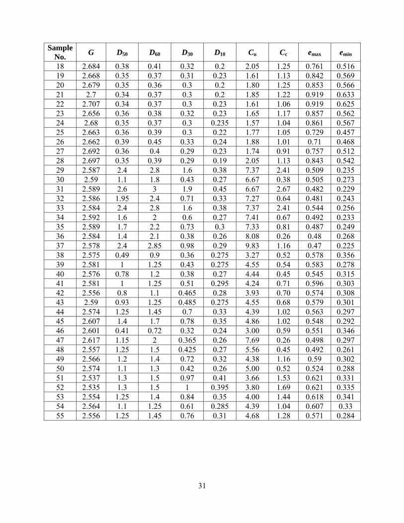
31

Sample No. G D50 D60 D30 D10 Cu Cc emax emin

18 2.684 0.38 0.41 0.32 0.2 2.05 1.25 0.761 0.516 19 2.668 0.35 0.37 0.31 0.23 1.61 1.13 0.842 0.569 20 2.679 0.35 0.36 0.3 0.2 1.80 1.25 0.853 0.566 21 2.7 0.34 0.37 0.3 0.2 1.85 1.22 0.919 0.633 22 2.707 0.34 0.37 0.3 0.23 1.61 1.06 0.919 0.625 23 2.656 0.36 0.38 0.32 0.23 1.65 1.17 0.857 0.562 24 2.68 0.35 0.37 0.3 0.235 1.57 1.04 0.861 0.567 25 2.663 0.36 0.39 0.3 0.22 1.77 1.05 0.729 0.457 26 2.662 0.39 0.45 0.33 0.24 1.88 1.01 0.71 0.468 27 2.692 0.36 0.4 0.29 0.23 1.74 0.91 0.757 0.512 28 2.697 0.35 0.39 0.29 0.19 2.05 1.13 0.843 0.542 29 2.587 2.4 2.8 1.6 0.38 7.37 2.41 0.509 0.235 30 2.59 1.1 1.8 0.43 0.27 6.67 0.38 0.505 0.273 31 2.589 2.6 3 1.9 0.45 6.67 2.67 0.482 0.229 32 2.586 1.95 2.4 0.71 0.33 7.27 0.64 0.481 0.243 33 2.584 2.4 2.8 1.6 0.38 7.37 2.41 0.544 0.256 34 2.592 1.6 2 0.6 0.27 7.41 0.67 0.492 0.233 35 2.589 1.7 2.2 0.73 0.3 7.33 0.81 0.487 0.249 36 2.584 1.4 2.1 0.38 0.26 8.08 0.26 0.48 0.268 37 2.578 2.4 2.85 0.98 0.29 9.83 1.16 0.47 0.225 38 2.575 0.49 0.9 0.36 0.275 3.27 0.52 0.578 0.356 39 2.581 1 1.25 0.43 0.275 4.55 0.54 0.583 0.278 40 2.576 0.78 1.2 0.38 0.27 4.44 0.45 0.545 0.315 41 2.581 1 1.25 0.51 0.295 4.24 0.71 0.596 0.303 42 2.556 0.8 1.1 0.465 0.28 3.93 0.70 0.574 0.308 43 2.59 0.93 1.25 0.485 0.275 4.55 0.68 0.579 0.301 44 2.574 1.25 1.45 0.7 0.33 4.39 1.02 0.563 0.297 45 2.607 1.4 1.7 0.78 0.35 4.86 1.02 0.548 0.292 46 2.601 0.41 0.72 0.32 0.24 3.00 0.59 0.551 0.346 47 2.617 1.15 2 0.365 0.26 7.69 0.26 0.498 0.297 48 2.557 1.25 1.5 0.425 0.27 5.56 0.45 0.492 0.261 49 2.566 1.2 1.4 0.72 0.32 4.38 1.16 0.59 0.302 50 2.574 1.1 1.3 0.42 0.26 5.00 0.52 0.524 0.288 51 2.537 1.3 1.5 0.97 0.41 3.66 1.53 0.621 0.331 52 2.535 1.3 1.5 1 0.395 3.80 1.69 0.621 0.335 53 2.554 1.25 1.4 0.84 0.35 4.00 1.44 0.618 0.341 54 2.564 1.1 1.25 0.61 0.285 4.39 1.04 0.607 0.33 55 2.556 1.25 1.45 0.76 0.31 4.68 1.28 0.571 0.284

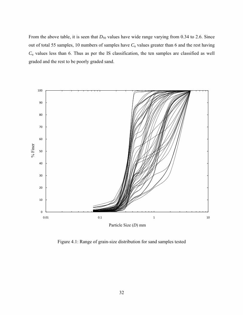
32

From the above table, it is seen that D50 values have wide range varying from 0.34 to 2.6. Since

out of total 55 samples, 10 numbers of samples have Cu values greater than 6 and the rest having

Cu values less than 6. Thus as per the IS classification, the ten samples are classified as well

graded and the rest to be poorly graded sand.

Figure 4.1: Range of grain-size distribution for sand samples tested

0

10

20

30

40

50

60

70

80

90

100

0.01 0.1 1 10

% F

iner

Particle Size (D) mm

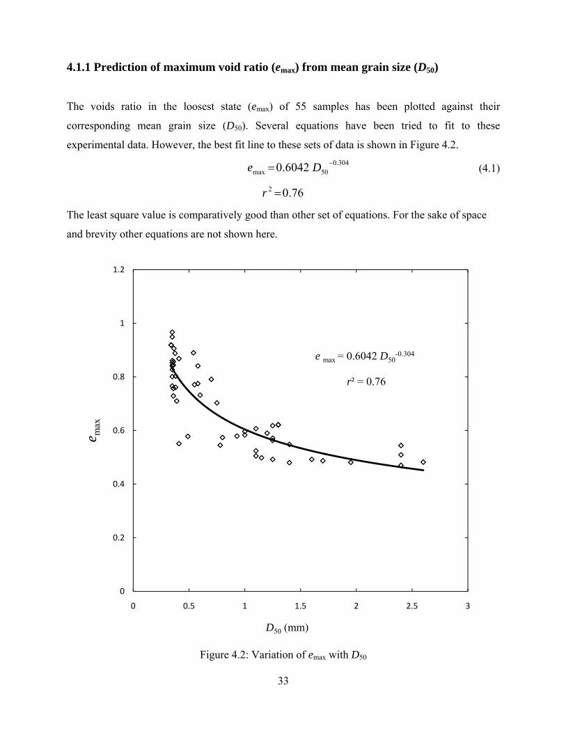
33

4.1.1 Prediction of maximum void ratio (emax) from mean grain size (D50)

The voids ratio in the loosest state (emax) of 55 samples has been plotted against their

corresponding mean grain size (D50). Several equations have been tried to fit to these

experimental data. However, the best fit line to these sets of data is shown in Figure 4.2.

304.050max 6042.0 −= De

(4.1)

76.02 =r

The least square value is comparatively good than other set of equations. For the sake of space

and brevity other equations are not shown here.

Figure 4.2: Variation of emax with D50

e max = 0.6042 D50-0.304

r² = 0.76

0

0.2

0.4

0.6

0.8

1

1.2

0 0.5 1 1.5 2 2.5 3

e max

D50 (mm)

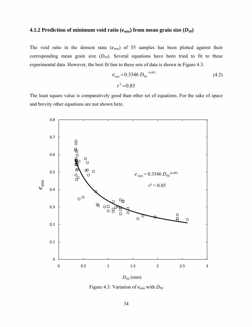
34

4.1.2 Prediction of minimum void ratio (emin) from mean grain size (D50)

The void ratio in the densest state (emin) of 55 samples has been plotted against their

corresponding mean grain size (D50). Several equations have been tried to fit to these

experimental data. However, the best fit line to these sets of data is shown in Figure 4.3. 491.0

50min 3346.0 −= De

(4.2)

85.02 =r

The least square value is comparatively good than other set of equations. For the sake of space

and brevity other equations are not shown here.

Figure 4.3: Variation of emin with D50

e min = 0.3346 D50-0.491

r² = 0.85

0

0.1

0.2

0.3

0.4

0.5

0.6

0.7

0.8

0 0.5 1 1.5 2 2.5 3

e min

D50 (mm)

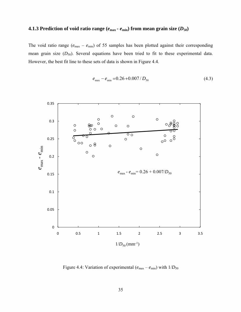
35

4.1.3 Prediction of void ratio range (emax - emin) from mean grain size (D50)

The void ratio range (emax – emin) of 55 samples has been plotted against their corresponding

mean grain size (D50). Several equations have been tried to fit to these experimental data.

However, the best fit line to these sets of data is shown in Figure 4.4.

50minmax /007.026.0 Dee +=−

(4.3)

Figure 4.4: Variation of experimental (emax – emin) with 1/D50

emax - emin= 0.26 + 0.007/D50

0

0.05

0.1

0.15

0.2

0.25

0.3

0.35

0 0.5 1 1.5 2 2.5 3 3.5

e max

-e m

in

1/D50 (mm-1)

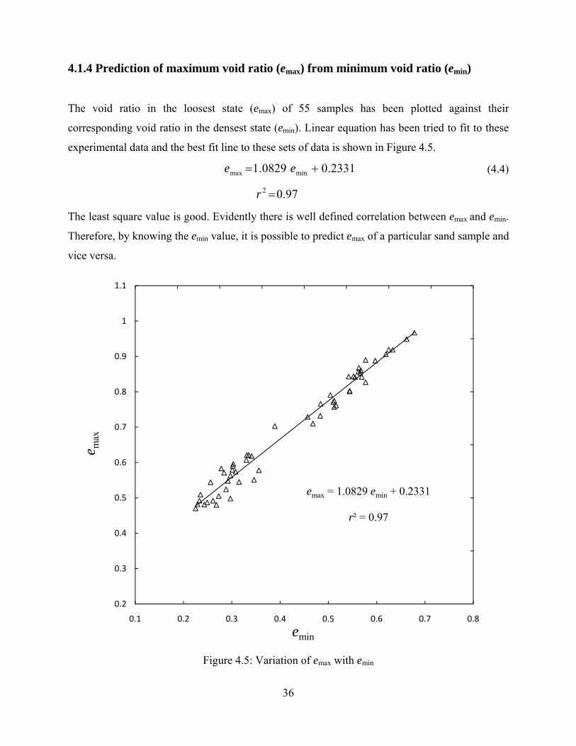
36

4.1.4 Prediction of maximum void ratio (emax) from minimum void ratio (emin)

The void ratio in the loosest state (emax) of 55 samples has been plotted against their

corresponding void ratio in the densest state (emin). Linear equation has been tried to fit to these

experimental data and the best fit line to these sets of data is shown in Figure 4.5.

2331.00829.1 minmax += ee

(4.4)

97.02 =r

The least square value is good. Evidently there is well defined correlation between emax and emin.

Therefore, by knowing the emin value, it is possible to predict emax of a particular sand sample and

vice versa.

Figure 4.5: Variation of emax with emin

emax = 1.0829 emin + 0.2331

r² = 0.97

0.2

0.3

0.4

0.5

0.6

0.7

0.8

0.9

1

1.1

0.1 0.2 0.3 0.4 0.5 0.6 0.7 0.8

e max

emin

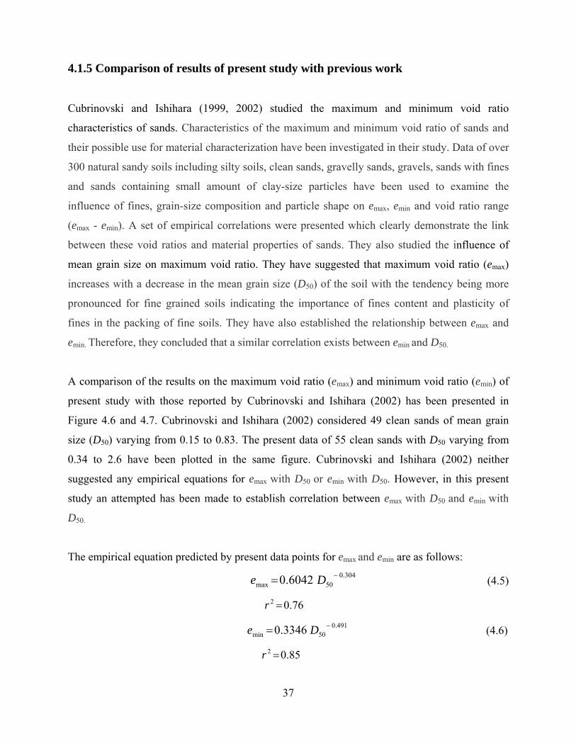
37

4.1.5 Comparison of results of present study with previous work

Cubrinovski and Ishihara (1999, 2002) studied the maximum and minimum void ratio

characteristics of sands. Characteristics of the maximum and minimum void ratio of sands and

their possible use for material characterization have been investigated in their study. Data of over

300 natural sandy soils including silty soils, clean sands, gravelly sands, gravels, sands with fines

and sands containing small amount of clay-size particles have been used to examine the

influence of fines, grain-size composition and particle shape on emax, emin and void ratio range

(emax - emin). A set of empirical correlations were presented which clearly demonstrate the link

between these void ratios and material properties of sands. They also studied the influence of

mean grain size on maximum void ratio. They have suggested that maximum void ratio (emax)

increases with a decrease in the mean grain size (D50) of the soil with the tendency being more

pronounced for fine grained soils indicating the importance of fines content and plasticity of

fines in the packing of fine soils. They have also established the relationship between emax and

emin. Therefore, they concluded that a similar correlation exists between emin and D50.

A comparison of the results on the maximum void ratio (emax) and minimum void ratio (emin) of

present study with those reported by Cubrinovski and Ishihara (2002) has been presented in

Figure 4.6 and 4.7. Cubrinovski and Ishihara (2002) considered 49 clean sands of mean grain

size (D50) varying from 0.15 to 0.83. The present data of 55 clean sands with D50 varying from

0.34 to 2.6 have been plotted in the same figure. Cubrinovski and Ishihara (2002) neither

suggested any empirical equations for emax with D50 or emin with D50. However, in this present

study an attempted has been made to establish correlation between emax with D50 and emin with

D50.

The empirical equation predicted by present data points for emax and emin are as follows:

304.0

50max 6042.0 −= De

(4.5)

76.02 =r

491.0

50min 3346.0 −= De

(4.6)

85.02 =r

38

Figure 4.6: Present test data points along with the data points of Cubrinovski and Ishihara (2002)

for emax with D50

emax = 0.6042 D50- 0.304

r² = 0.76

0.2

0.4

0.6

0.8

1

1.2

1.4

1.6

1.8

0 0.5 1 1.5 2 2.5 3

e max

D50 (mm)

Cubrivovski & Ishihara (2002)Data Points( 49 clean sand samples with D50 varyingfrom 0.15 mm to 0.83 mm)

Note: Cubrivnovski & Ishihara (2002) didn't suggest any equations

Present Study Data Points( 55 clean sand samples with D50 varyingfrom 0.34 mm to 2.6 mm)

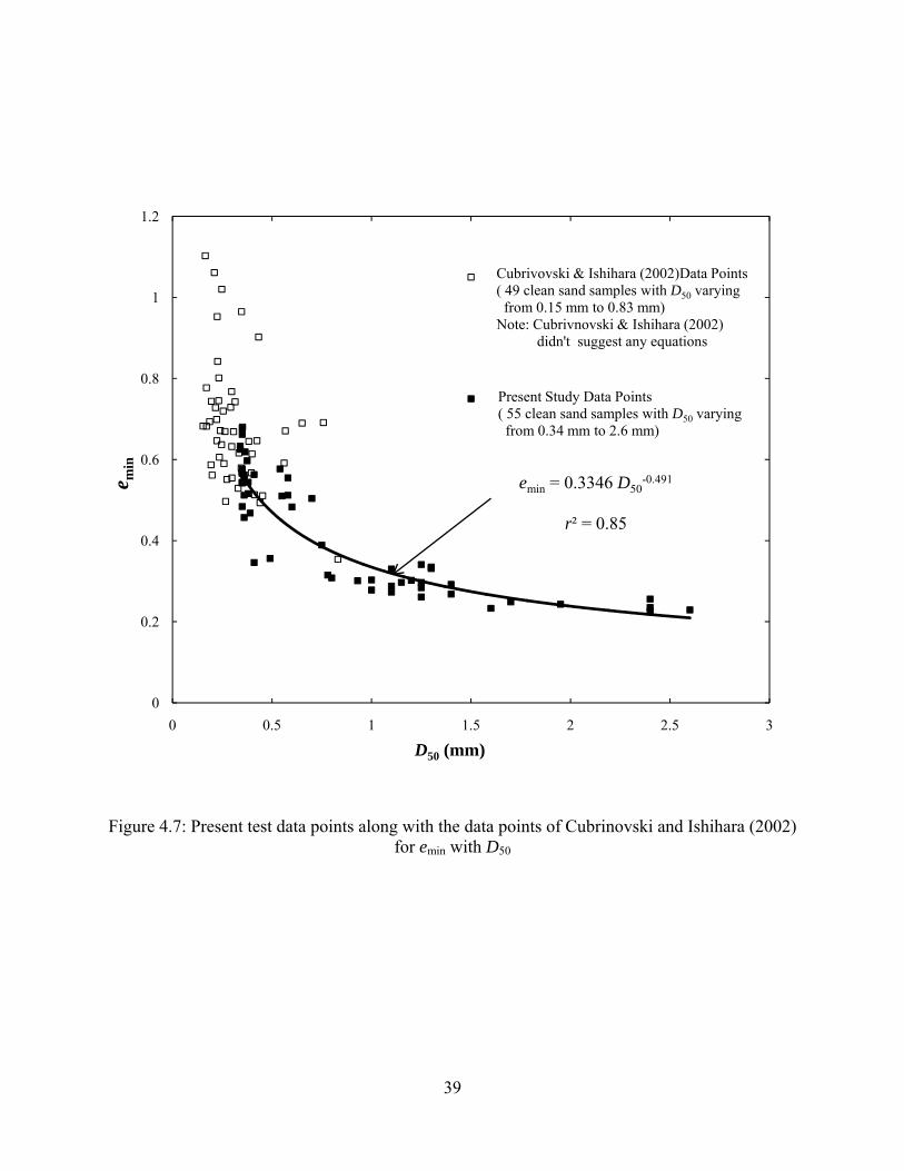
39

Figure 4.7: Present test data points along with the data points of Cubrinovski and Ishihara (2002) for emin with D50

emin = 0.3346 D50-0.491

r² = 0.85

0

0.2

0.4

0.6

0.8

1

1.2

0 0.5 1 1.5 2 2.5 3

e min

D50 (mm)

Cubrivovski & Ishihara (2002)Data Points( 49 clean sand samples with D50 varyingfrom 0.15 mm to 0.83 mm)

Note: Cubrivnovski & Ishihara (2002) didn't suggest any equations

Present Study Data Points( 55 clean sand samples with D50 varyingfrom 0.34 mm to 2.6 mm)

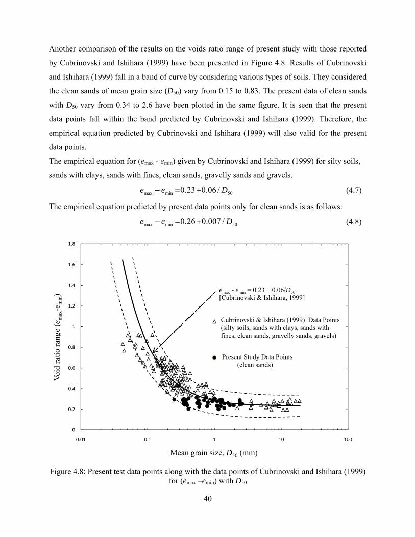
Another

by Cubri

and Ishih

the clean

with D50

data poin

empirica

data poin

The emp

sands wit

The emp

Figure 4

0

0.2

0.4

0.6

0.8

1

1.2

1.4

1.6

1.8

0

Void

ratio

rang

e (e

max

-em

in)

comparison

inovski and

hara (1999) f

n sands of m

vary from 0

nts fall with

l equation p

nts.

irical equati

th clays, san

irical equati

.8: Present te

0.01

of the resul

Ishihara (19

fall in a band

mean grain siz

0.34 to 2.6 h

hin the band

predicted by

on for (emax

nds with fine

maxe −

on predicted

maxe −

est data poin

0.1

lts on the vo

999) have be

d of curve by

ze (D50) var

have been p

d predicted b

Cubrinovsk

- emin) given

es, clean sand

min 23.0e =−

d by present

min 26.0e =−

nts along witfor (emax

Mean g

40

oids ratio ran

een presente

y considerin

ry from 0.15

plotted in the

by Cubrinov

ki and Ishiha

n by Cubrino

ds, gravelly

50/06.03 D+

data points o

5/007.06 D+

th the data px –emin) with

1

grain size, D5

emax -[Cubr

Cubr(siltyfines

Pres

nge of prese

ed in Figure

ng various typ

to 0.83. Th

e same figur

vski and Ish

ara (1999) w

ovski and Ish

sands and gr

only for clea

50

oints of Cubh D50

50 (mm)

- emin = 0.23 + rinovski & Ish

rinovski & Ishiy soils, sands ws, clean sands,

sent Study Data(clean sands)

ent study wi

e 4.8. Result

pes of soils.

he present da

re. It is seen

hihara (1999

will also vali

hihara (1999

ravels.

an sands is a

brinovski and

10

0.06/D50hihara, 1999]

ihara (1999) Dwith clays, sandgravelly sands

a Points)

th those rep

ts of Cubrino

They consid

ata of clean s

n that the pr

9). Therefore

id for the pr

9) for silty so

(4

as follows:

(4

d Ishihara (1

10

Data Pointsds with s, gravels)

ported

ovski

dered

sands

resent

e, the

resent

oils,

4.7)

4.8)

1999)

0

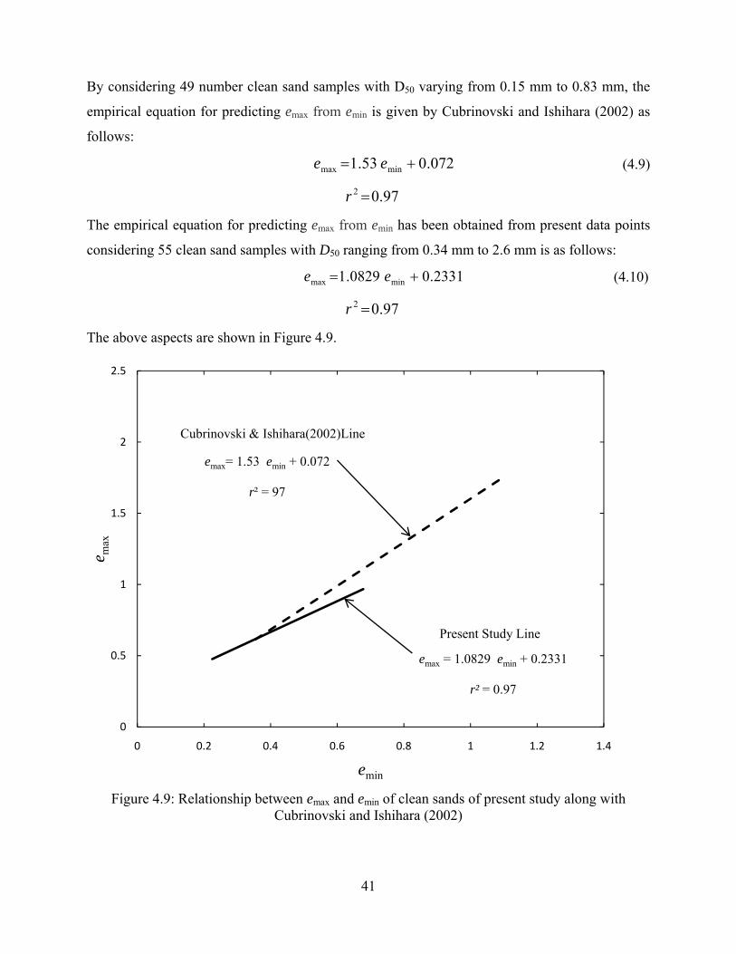
41

By considering 49 number clean sand samples with D50 varying from 0.15 mm to 0.83 mm, the

empirical equation for predicting emax from emin is given by Cubrinovski and Ishihara (2002) as

follows:

072.053.1 minmax += ee

(4.9)

97.02 =r

The empirical equation for predicting emax from emin has been obtained from present data points

considering 55 clean sand samples with D50 ranging from 0.34 mm to 2.6 mm is as follows:

2331.00829.1 minmax += ee

(4.10)

97.02 =r

The above aspects are shown in Figure 4.9.

Figure 4.9: Relationship between emax and emin of clean sands of present study along with

Cubrinovski and Ishihara (2002)

emax= 1.53 emin + 0.072

r² = 97

emax = 1.0829 emin + 0.2331

r² = 0.97

0

0.5

1

1.5

2

2.5

0 0.2 0.4 0.6 0.8 1 1.2 1.4

e max

emin

Cubrinovski & Ishihara(2002)Line

Present Study Line

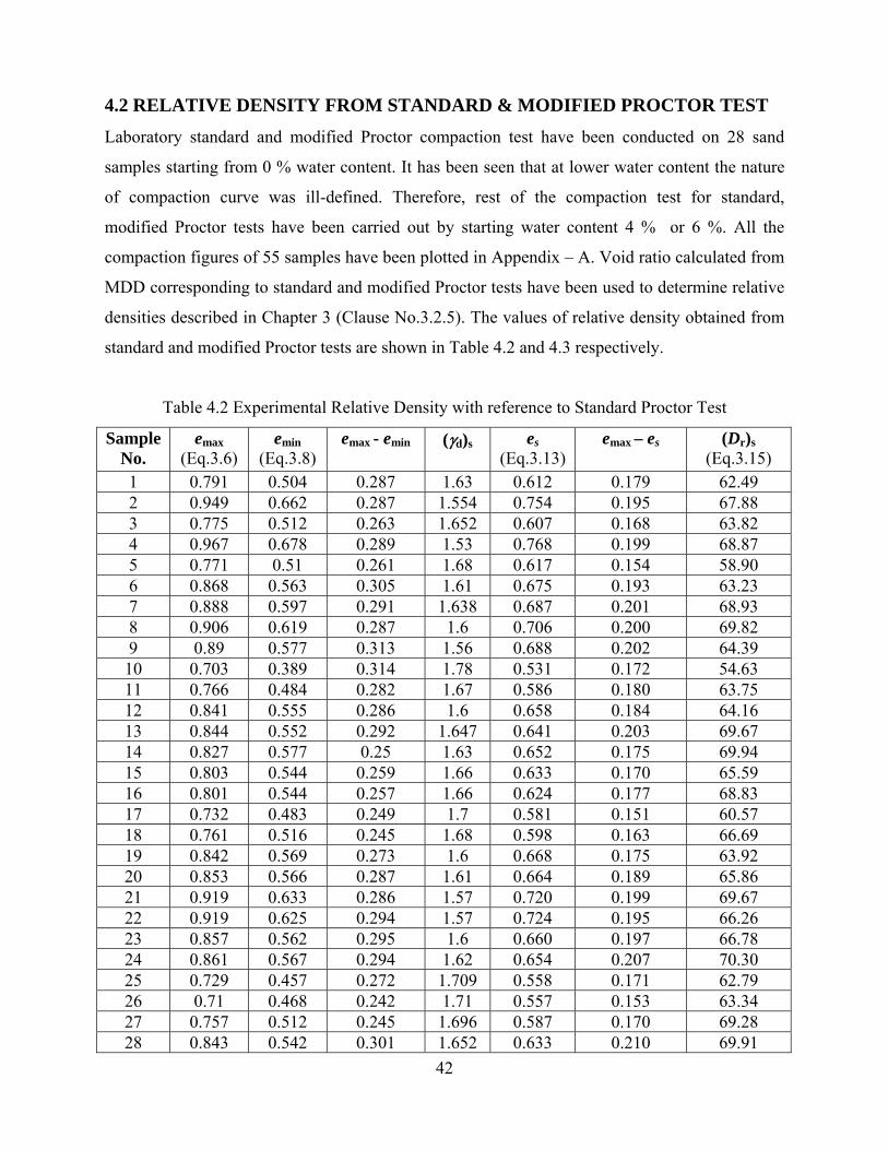
42

4.2 RELATIVE DENSITY FROM STANDARD & MODIFIED PROCTOR TEST

Laboratory standard and modified Proctor compaction test have been conducted on 28 sand

samples starting from 0 % water content. It has been seen that at lower water content the nature

of compaction curve was ill-defined. Therefore, rest of the compaction test for standard,

modified Proctor tests have been carried out by starting water content 4 % or 6 %. All the

compaction figures of 55 samples have been plotted in Appendix – A. Void ratio calculated from

MDD corresponding to standard and modified Proctor tests have been used to determine relative

densities described in Chapter 3 (Clause No.3.2.5). The values of relative density obtained from

standard and modified Proctor tests are shown in Table 4.2 and 4.3 respectively.

Table 4.2 Experimental Relative Density with reference to Standard Proctor Test

Sample No.

emax (Eq.3.6)

emin (Eq.3.8)

emax - emin (γd)s es (Eq.3.13)

emax – es (Dr)s (Eq.3.15)

1 0.791 0.504 0.287 1.63 0.612 0.179 62.49 2 0.949 0.662 0.287 1.554 0.754 0.195 67.88 3 0.775 0.512 0.263 1.652 0.607 0.168 63.82 4 0.967 0.678 0.289 1.53 0.768 0.199 68.87 5 0.771 0.51 0.261 1.68 0.617 0.154 58.90 6 0.868 0.563 0.305 1.61 0.675 0.193 63.23 7 0.888 0.597 0.291 1.638 0.687 0.201 68.93 8 0.906 0.619 0.287 1.6 0.706 0.200 69.82 9 0.89 0.577 0.313 1.56 0.688 0.202 64.39 10 0.703 0.389 0.314 1.78 0.531 0.172 54.63 11 0.766 0.484 0.282 1.67 0.586 0.180 63.75 12 0.841 0.555 0.286 1.6 0.658 0.184 64.16 13 0.844 0.552 0.292 1.647 0.641 0.203 69.67 14 0.827 0.577 0.25 1.63 0.652 0.175 69.94 15 0.803 0.544 0.259 1.66 0.633 0.170 65.59 16 0.801 0.544 0.257 1.66 0.624 0.177 68.83 17 0.732 0.483 0.249 1.7 0.581 0.151 60.57 18 0.761 0.516 0.245 1.68 0.598 0.163 66.69 19 0.842 0.569 0.273 1.6 0.668 0.175 63.92 20 0.853 0.566 0.287 1.61 0.664 0.189 65.86 21 0.919 0.633 0.286 1.57 0.720 0.199 69.67 22 0.919 0.625 0.294 1.57 0.724 0.195 66.26 23 0.857 0.562 0.295 1.6 0.660 0.197 66.78 24 0.861 0.567 0.294 1.62 0.654 0.207 70.30 25 0.729 0.457 0.272 1.709 0.558 0.171 62.79 26 0.71 0.468 0.242 1.71 0.557 0.153 63.34 27 0.757 0.512 0.245 1.696 0.587 0.170 69.28 28 0.843 0.542 0.301 1.652 0.633 0.210 69.91

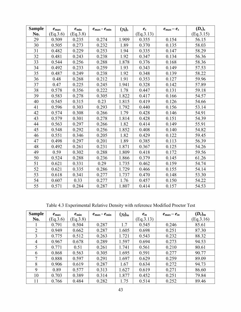
43

Sample No.

emax (Eq.3.6)

emin (Eq.3.8)

emax - emin (γd)s es (Eq.3.13)

emax – es (Dr)s (Eq.3.15)

29 0.509 0.235 0.274 1.909 0.355 0.154 56.15 30 0.505 0.273 0.232 1.89 0.370 0.135 58.03 31 0.482 0.229 0.253 1.94 0.335 0.147 58.29 32 0.481 0.243 0.238 1.92 0.347 0.134 56.36 33 0.544 0.256 0.288 1.878 0.376 0.168 58.36 34 0.492 0.233 0.259 1.93 0.343 0.149 57.53 35 0.487 0.249 0.238 1.92 0.348 0.139 58.22 36 0.48 0.268 0.212 1.91 0.353 0.127 59.96 37 0.47 0.225 0.245 1.941 0.328 0.142 57.89 38 0.578 0.356 0.222 1.78 0.447 0.131 59.18 39 0.583 0.278 0.305 1.822 0.417 0.166 54.57 40 0.545 0.315 0.23 1.815 0.419 0.126 54.66 41 0.596 0.303 0.293 1.792 0.440 0.156 53.14 42 0.574 0.308 0.266 1.79 0.428 0.146 54.91 43 0.579 0.301 0.278 1.814 0.428 0.151 54.39 44 0.563 0.297 0.266 1.82 0.414 0.149 55.91 45 0.548 0.292 0.256 1.852 0.408 0.140 54.82 46 0.551 0.346 0.205 1.82 0.429 0.122 59.45 47 0.498 0.297 0.201 1.89 0.385 0.113 56.39 48 0.492 0.261 0.231 1.871 0.367 0.125 54.26 49 0.59 0.302 0.288 1.809 0.418 0.172 59.56 50 0.524 0.288 0.236 1.866 0.379 0.145 61.26 51 0.621 0.331 0.29 1.735 0.462 0.159 54.74 52 0.621 0.335 0.286 1.729 0.466 0.155 54.14 53 0.618 0.341 0.277 1.737 0.470 0.148 53.30 54 0.607 0.33 0.277 1.76 0.457 0.150 54.22 55 0.571 0.284 0.287 1.807 0.414 0.157 54.53

Table 4.3 Experimental Relative Density with reference Modified Proctor Test

Sample No.

emax (Eq.3.6)

emin (Eq.3.8)

emax - emin (γd)m em (Eq.3.13)

emax – em (Dr)m (Eq.3.16)

1 0.791 0.504 0.287 1.7 0.545 0.246 85.61 2 0.949 0.662 0.287 1.605 0.698 0.251 87.30 3 0.775 0.512 0.263 1.721 0.543 0.232 88.32 4 0.967 0.678 0.289 1.597 0.694 0.273 94.53 5 0.771 0.51 0.261 1.741 0.561 0.210 80.61 6 0.868 0.563 0.305 1.695 0.591 0.277 90.77 7 0.888 0.597 0.291 1.697 0.629 0.259 89.09 8 0.906 0.619 0.287 1.67 0.634 0.272 94.73 9 0.89 0.577 0.313 1.627 0.619 0.271 86.60 10 0.703 0.389 0.314 1.877 0.452 0.251 79.84 11 0.766 0.484 0.282 1.75 0.514 0.252 89.46

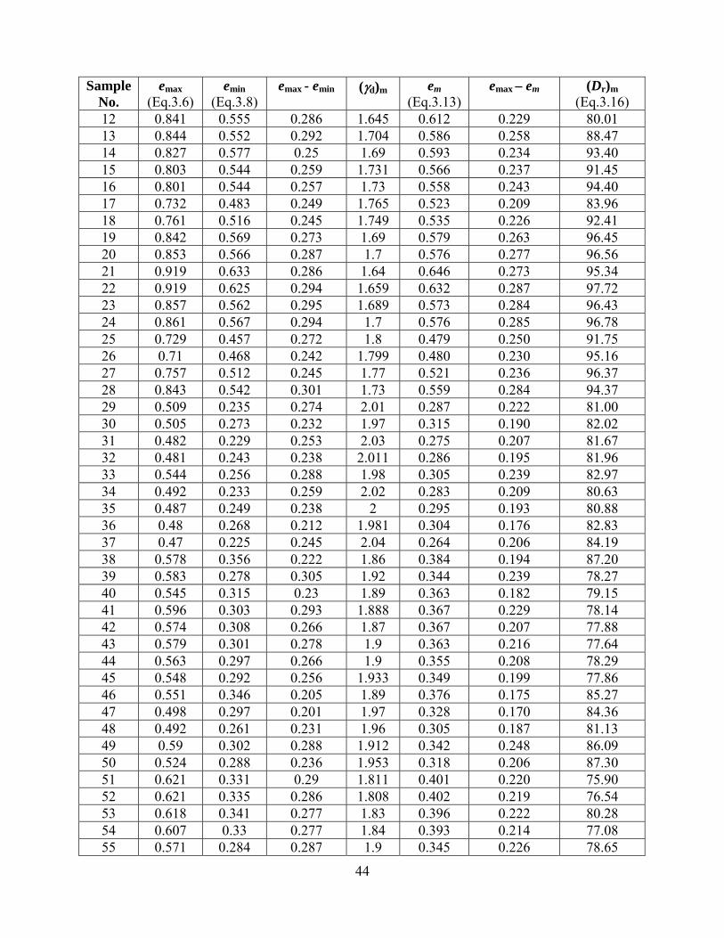
44

Sample No.

emax (Eq.3.6)

emin (Eq.3.8)

emax - emin (γd)m em (Eq.3.13)

emax – em (Dr)m (Eq.3.16)

12 0.841 0.555 0.286 1.645 0.612 0.229 80.01 13 0.844 0.552 0.292 1.704 0.586 0.258 88.47 14 0.827 0.577 0.25 1.69 0.593 0.234 93.40 15 0.803 0.544 0.259 1.731 0.566 0.237 91.45 16 0.801 0.544 0.257 1.73 0.558 0.243 94.40 17 0.732 0.483 0.249 1.765 0.523 0.209 83.96 18 0.761 0.516 0.245 1.749 0.535 0.226 92.41 19 0.842 0.569 0.273 1.69 0.579 0.263 96.45 20 0.853 0.566 0.287 1.7 0.576 0.277 96.56 21 0.919 0.633 0.286 1.64 0.646 0.273 95.34 22 0.919 0.625 0.294 1.659 0.632 0.287 97.72 23 0.857 0.562 0.295 1.689 0.573 0.284 96.43 24 0.861 0.567 0.294 1.7 0.576 0.285 96.78 25 0.729 0.457 0.272 1.8 0.479 0.250 91.75 26 0.71 0.468 0.242 1.799 0.480 0.230 95.16 27 0.757 0.512 0.245 1.77 0.521 0.236 96.37 28 0.843 0.542 0.301 1.73 0.559 0.284 94.37 29 0.509 0.235 0.274 2.01 0.287 0.222 81.00 30 0.505 0.273 0.232 1.97 0.315 0.190 82.02 31 0.482 0.229 0.253 2.03 0.275 0.207 81.67 32 0.481 0.243 0.238 2.011 0.286 0.195 81.96 33 0.544 0.256 0.288 1.98 0.305 0.239 82.97 34 0.492 0.233 0.259 2.02 0.283 0.209 80.63 35 0.487 0.249 0.238 2 0.295 0.193 80.88 36 0.48 0.268 0.212 1.981 0.304 0.176 82.83 37 0.47 0.225 0.245 2.04 0.264 0.206 84.19 38 0.578 0.356 0.222 1.86 0.384 0.194 87.20 39 0.583 0.278 0.305 1.92 0.344 0.239 78.27 40 0.545 0.315 0.23 1.89 0.363 0.182 79.15 41 0.596 0.303 0.293 1.888 0.367 0.229 78.14 42 0.574 0.308 0.266 1.87 0.367 0.207 77.88 43 0.579 0.301 0.278 1.9 0.363 0.216 77.64 44 0.563 0.297 0.266 1.9 0.355 0.208 78.29 45 0.548 0.292 0.256 1.933 0.349 0.199 77.86 46 0.551 0.346 0.205 1.89 0.376 0.175 85.27 47 0.498 0.297 0.201 1.97 0.328 0.170 84.36 48 0.492 0.261 0.231 1.96 0.305 0.187 81.13 49 0.59 0.302 0.288 1.912 0.342 0.248 86.09 50 0.524 0.288 0.236 1.953 0.318 0.206 87.30 51 0.621 0.331 0.29 1.811 0.401 0.220 75.90 52 0.621 0.335 0.286 1.808 0.402 0.219 76.54 53 0.618 0.341 0.277 1.83 0.396 0.222 80.28 54 0.607 0.33 0.277 1.84 0.393 0.214 77.08 55 0.571 0.284 0.287 1.9 0.345 0.226 78.65

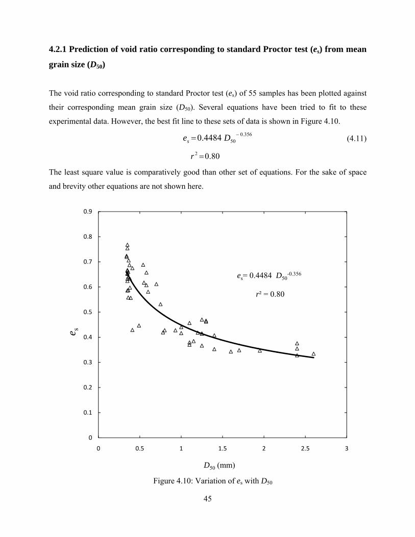
45

4.2.1 Prediction of void ratio corresponding to standard Proctor test (es) from mean

grain size (D50)

The void ratio corresponding to standard Proctor test (es) of 55 samples has been plotted against

their corresponding mean grain size (D50). Several equations have been tried to fit to these

experimental data. However, the best fit line to these sets of data is shown in Figure 4.10. 356.0

504484.0 −= Des

(4.11)

80.02 =r

The least square value is comparatively good than other set of equations. For the sake of space

and brevity other equations are not shown here.

Figure 4.10: Variation of es with D50

es= 0.4484 D50-0.356

r² = 0.80

0

0.1

0.2

0.3

0.4

0.5

0.6

0.7

0.8

0.9

0 0.5 1 1.5 2 2.5 3

e s

D50 (mm)

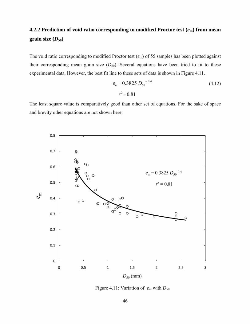
46

4.2.2 Prediction of void ratio corresponding to modified Proctor test (em) from mean

grain size (D50)

The void ratio corresponding to modified Proctor test (em) of 55 samples has been plotted against

their corresponding mean grain size (D50). Several equations have been tried to fit to these

experimental data. However, the best fit line to these sets of data is shown in Figure 4.11. 4.0

503825.0 −= Dem

(4.12)

81.02 =r

The least square value is comparatively good than other set of equations. For the sake of space

and brevity other equations are not shown here.

Figure 4.11: Variation of em with D50

em = 0.3825 D50-0.4

r² = 0.81

0

0.1

0.2

0.3

0.4

0.5

0.6

0.7

0.8

0 0.5 1 1.5 2 2.5 3

e m

D50 (mm)

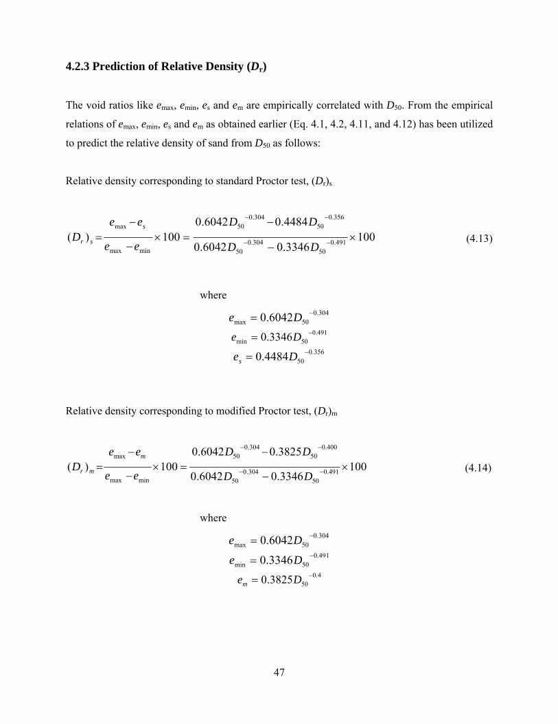
47

4.2.3 Prediction of Relative Density (Dr)

The void ratios like emax, emin, es and em are empirically correlated with D50. From the empirical

relations of emax, emin, es and em as obtained earlier (Eq. 4.1, 4.2, 4.11, and 4.12) has been utilized

to predict the relative density of sand from D50 as follows:

Relative density corresponding to standard Proctor test, (Dr)s

1003346.06042.0

4484.06042.0100)( 491.0

50304.0

50

356.050

304.050

minmax

max

×−

−=×

−

−= −−

−−

DD

DD

ee

eeD

s

sr

(4.13)

where 304.0

50max 6042.0 −= De 491.0

50min 3346.0 −= De 356.0

504484.0 −= Des

Relative density corresponding to modified Proctor test, (Dr)m

1003346.06042.0

3825.06042.0100)( 491.0

50304.0

50

400.050

304.050

minmax

max

×−

−=×

−

−= −−

−−

DD

DD

ee

eeD

m

mr

(4.14)

where 304.0

50max 6042.0 −= De 491.0

50min 3346.0 −= De 4.0

503825.0 −= Dem

48

The relative density predicted by conducting Standard and Modified Proctors tests by using Eq.

(4.13, 4.14) are shown in Table 4.4 and Table 4.5 respectively.

Table 4.4: Predicted Relative Density with reference Standard Proctor Test

Sample No.

Predicted emax

Predicted emin

Predicted emax - emin

Predicted es

Predicted emax – es

Predicted (Dr)s (%)

1 0.673 0.399 0.275 0.509 0.164 59.79 2 0.831 0.560 0.271 0.652 0.180 66.31 3 0.713 0.437 0.276 0.544 0.169 61.15 4 0.831 0.560 0.271 0.652 0.180 66.31 5 0.725 0.449 0.276 0.555 0.170 61.58 6 0.792 0.518 0.274 0.616 0.176 64.40 7 0.814 0.542 0.272 0.636 0.178 65.44 8 0.821 0.549 0.272 0.642 0.179 65.77 9 0.729 0.453 0.276 0.558 0.170 61.73 10 0.659 0.385 0.274 0.497 0.163 59.35 11 0.831 0.560 0.271 0.652 0.180 66.31 12 0.713 0.437 0.276 0.544 0.169 61.15 13 0.824 0.553 0.272 0.645 0.179 65.94 14 0.831 0.560 0.271 0.652 0.180 66.31 15 0.811 0.538 0.273 0.633 0.178 65.28 16 0.831 0.560 0.271 0.652 0.180 66.31 17 0.706 0.430 0.276 0.538 0.168 60.89 18 0.811 0.538 0.273 0.633 0.178 65.28 19 0.831 0.560 0.271 0.652 0.180 66.31 20 0.831 0.560 0.271 0.652 0.180 66.31 21 0.839 0.568 0.270 0.658 0.180 66.69 22 0.839 0.568 0.270 0.658 0.180 66.69 23 0.824 0.553 0.272 0.645 0.179 65.94 24 0.831 0.560 0.271 0.652 0.180 66.31 25 0.824 0.553 0.272 0.645 0.179 65.94 26 0.804 0.531 0.273 0.627 0.177 64.97 27 0.824 0.553 0.272 0.645 0.179 65.94 28 0.831 0.560 0.271 0.652 0.180 66.31 29 0.463 0.218 0.245 0.328 0.135 54.90 30 0.587 0.319 0.268 0.433 0.154 57.35 31 0.452 0.209 0.243 0.319 0.133 54.74 32 0.493 0.241 0.252 0.354 0.140 55.39 33 0.463 0.218 0.245 0.328 0.135 54.90 34 0.524 0.266 0.258 0.379 0.144 55.96 35 0.514 0.258 0.256 0.371 0.143 55.78 36 0.545 0.284 0.262 0.398 0.148 56.41 37 0.463 0.218 0.245 0.328 0.135 54.90

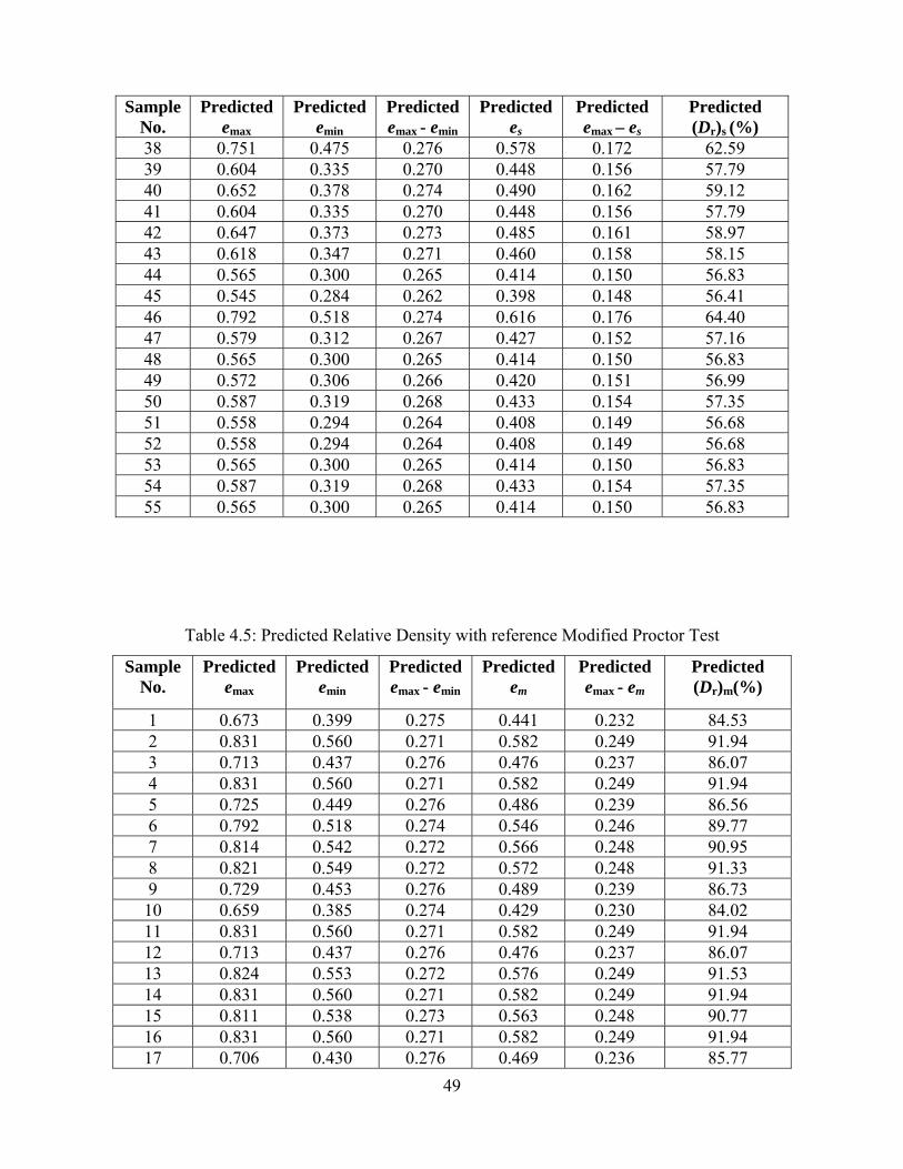
49

Sample No.

Predicted emax

Predicted emin

Predicted emax - emin

Predicted es

Predicted emax – es

Predicted (Dr)s (%)

38 0.751 0.475 0.276 0.578 0.172 62.59 39 0.604 0.335 0.270 0.448 0.156 57.79 40 0.652 0.378 0.274 0.490 0.162 59.12 41 0.604 0.335 0.270 0.448 0.156 57.79 42 0.647 0.373 0.273 0.485 0.161 58.97 43 0.618 0.347 0.271 0.460 0.158 58.15 44 0.565 0.300 0.265 0.414 0.150 56.83 45 0.545 0.284 0.262 0.398 0.148 56.41 46 0.792 0.518 0.274 0.616 0.176 64.40 47 0.579 0.312 0.267 0.427 0.152 57.16 48 0.565 0.300 0.265 0.414 0.150 56.83 49 0.572 0.306 0.266 0.420 0.151 56.99 50 0.587 0.319 0.268 0.433 0.154 57.35 51 0.558 0.294 0.264 0.408 0.149 56.68 52 0.558 0.294 0.264 0.408 0.149 56.68 53 0.565 0.300 0.265 0.414 0.150 56.83 54 0.587 0.319 0.268 0.433 0.154 57.35 55 0.565 0.300 0.265 0.414 0.150 56.83

Table 4.5: Predicted Relative Density with reference Modified Proctor Test

Sample No.

Predicted emax

Predicted emin

Predicted emax - emin

Predicted em

Predicted emax - em

Predicted (Dr)m(%)

1 0.673 0.399 0.275 0.441 0.232 84.53 2 0.831 0.560 0.271 0.582 0.249 91.94 3 0.713 0.437 0.276 0.476 0.237 86.07 4 0.831 0.560 0.271 0.582 0.249 91.94 5 0.725 0.449 0.276 0.486 0.239 86.56 6 0.792 0.518 0.274 0.546 0.246 89.77 7 0.814 0.542 0.272 0.566 0.248 90.95 8 0.821 0.549 0.272 0.572 0.248 91.33 9 0.729 0.453 0.276 0.489 0.239 86.73 10 0.659 0.385 0.274 0.429 0.230 84.02 11 0.831 0.560 0.271 0.582 0.249 91.94 12 0.713 0.437 0.276 0.476 0.237 86.07 13 0.824 0.553 0.272 0.576 0.249 91.53 14 0.831 0.560 0.271 0.582 0.249 91.94 15 0.811 0.538 0.273 0.563 0.248 90.77 16 0.831 0.560 0.271 0.582 0.249 91.94 17 0.706 0.430 0.276 0.469 0.236 85.77

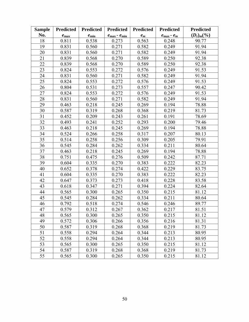
50

Sample No.

Predicted emax

Predicted emin

Predicted emax - emin

Predicted em

Predicted emax - em

Predicted (Dr)m(%)

18 0.811 0.538 0.273 0.563 0.248 90.77 19 0.831 0.560 0.271 0.582 0.249 91.94 20 0.831 0.560 0.271 0.582 0.249 91.94 21 0.839 0.568 0.270 0.589 0.250 92.38 22 0.839 0.568 0.270 0.589 0.250 92.38 23 0.824 0.553 0.272 0.576 0.249 91.53 24 0.831 0.560 0.271 0.582 0.249 91.94 25 0.824 0.553 0.272 0.576 0.249 91.53 26 0.804 0.531 0.273 0.557 0.247 90.42 27 0.824 0.553 0.272 0.576 0.249 91.53 28 0.831 0.560 0.271 0.582 0.249 91.94 29 0.463 0.218 0.245 0.269 0.194 78.88 30 0.587 0.319 0.268 0.368 0.219 81.73 31 0.452 0.209 0.243 0.261 0.191 78.69 32 0.493 0.241 0.252 0.293 0.200 79.46 33 0.463 0.218 0.245 0.269 0.194 78.88 34 0.524 0.266 0.258 0.317 0.207 80.13 35 0.514 0.258 0.256 0.309 0.205 79.91 36 0.545 0.284 0.262 0.334 0.211 80.64 37 0.463 0.218 0.245 0.269 0.194 78.88 38 0.751 0.475 0.276 0.509 0.242 87.71 39 0.604 0.335 0.270 0.383 0.222 82.23 40 0.652 0.378 0.274 0.422 0.229 83.75 41 0.604 0.335 0.270 0.383 0.222 82.23 42 0.647 0.373 0.273 0.418 0.228 83.58 43 0.618 0.347 0.271 0.394 0.224 82.64 44 0.565 0.300 0.265 0.350 0.215 81.12 45 0.545 0.284 0.262 0.334 0.211 80.64 46 0.792 0.518 0.274 0.546 0.246 89.77 47 0.579 0.312 0.267 0.362 0.217 81.51 48 0.565 0.300 0.265 0.350 0.215 81.12 49 0.572 0.306 0.266 0.356 0.216 81.31 50 0.587 0.319 0.268 0.368 0.219 81.73 51 0.558 0.294 0.264 0.344 0.213 80.95 52 0.558 0.294 0.264 0.344 0.213 80.95 53 0.565 0.300 0.265 0.350 0.215 81.12 54 0.587 0.319 0.268 0.368 0.219 81.73 55 0.565 0.300 0.265 0.350 0.215 81.12

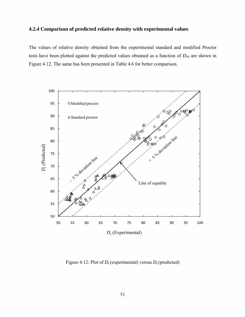
51

4.2.4 Comparison of predicted relative density with experimental values

The values of relative density obtained from the experimental standard and modified Proctor

tests have been plotted against the predicted values obtained as a function of D50 are shown in

Figure 4.12. The same has been presented in Table 4.6 for better comparison.

Figure 4.12: Plot of Dr (experimental) versus Dr (predicted)

50

55

60

65

70

75

80

85

90

95

100

50 55 60 65 70 75 80 85 90 95 100

Dr(P

redi

cted

)

Dr (Experimental)

Modified proctor

Standard proctor

Line of equality

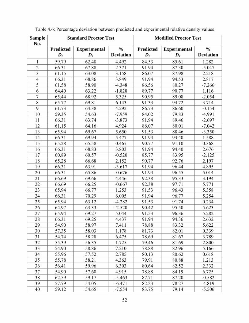
52

Table 4.6: Percentage deviation between predicted and experimental relative density values Sample

No. Standard Proctor Test Modified Proctor Test

Predicted Dr

Experimental Dr

% Deviation

Predicted Dr

Experimental Dr

% Deviation

1 59.79 62.48 4.492 84.53 85.61 1.282 2 66.31 67.88 2.371 91.94 87.30 -5.047 3 61.15 63.08 3.158 86.07 87.98 2.218 4 66.31 68.86 3.849 91.94 94.53 2.817 5 61.58 58.90 -4.348 86.56 80.27 -7.266 6 64.40 63.22 -1.828 89.77 90.77 1.116 7 65.44 68.92 5.325 90.95 89.08 -2.054 8 65.77 69.81 6.143 91.33 94.72 3.714 9 61.73 64.38 4.292 86.73 86.60 -0.154 10 59.35 54.63 -7.959 84.02 79.83 -4.991 11 66.31 63.74 -3.873 91.94 89.46 -2.697 12 61.15 64.16 4.924 86.07 80.01 -7.042 13 65.94 69.67 5.650 91.53 88.46 -3.350 14 66.31 69.94 5.477 91.94 93.40 1.588 15 65.28 65.58 0.467 90.77 91.10 0.368 16 66.31 68.83 3.803 91.94 94.40 2.676 17 60.89 60.57 -0.520 85.77 83.95 -2.125 18 65.28 66.68 2.152 90.77 92.76 2.197 19 66.31 63.91 -3.617 91.94 96.44 4.895 20 66.31 65.86 -0.676 91.94 96.55 5.014 21 66.69 69.66 4.446 92.38 95.33 3.194 22 66.69 66.25 -0.667 92.38 97.71 5.771 23 65.94 66.77 1.253 91.53 96.43 5.358 24 66.31 70.29 6.005 91.94 96.77 5.254 25 65.94 63.12 -4.282 91.53 91.74 0.234 26 64.97 63.33 -2.520 90.42 95.50 5.623 27 65.94 69.27 5.044 91.53 96.36 5.282 28 66.31 69.25 4.437 91.94 94.36 2.632 29 54.90 58.97 7.411 78.88 83.32 5.622 30 57.35 58.03 1.178 81.73 82.01 0.339 31 54.74 58.28 6.475 78.69 81.67 3.789 32 55.39 56.35 1.725 79.46 81.69 2.800 33 54.90 58.86 7.210 78.88 82.96 5.166 34 55.96 57.52 2.785 80.13 80.62 0.618 35 55.78 58.21 4.363 79.91 80.88 1.213 36 56.41 59.96 6.303 80.64 82.52 2.332 37 54.90 57.60 4.915 78.88 84.19 6.725 38 62.59 59.17 -5.463 87.71 87.20 -0.582 39 57.79 54.05 -6.471 82.23 78.27 -4.819 40 59.12 54.65 -7.554 83.75 79.14 -5.506

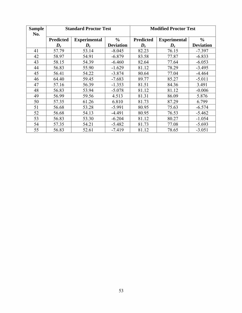
53

Sample No.

Standard Proctor Test

Modified Proctor Test

Predicted Dr

Experimental Dr

% Deviation

Predicted Dr

Experimental Dr

% Deviation

41 57.79 53.14 -8.045 82.23 76.15 -7.397 42 58.97 54.91 -6.879 83.58 77.87 -6.833 43 58.15 54.39 -6.460 82.64 77.64 -6.053 44 56.83 55.90 -1.629 81.12 78.29 -3.495 45 56.41 54.22 -3.874 80.64 77.04 -4.464 46 64.40 59.45 -7.683 89.77 85.27 -5.011 47 57.16 56.39 -1.353 81.51 84.36 3.491 48 56.83 53.94 -5.078 81.12 81.12 -0.006 49 56.99 59.56 4.513 81.31 86.09 5.876 50 57.35 61.26 6.810 81.73 87.29 6.799 51 56.68 53.28 -5.991 80.95 75.63 -6.574 52 56.68 54.13 -4.491 80.95 76.53 -5.462 53 56.83 53.30 -6.204 81.12 80.27 -1.054 54 57.35 54.21 -5.482 81.73 77.08 -5.693 55 56.83 52.61 -7.419 81.12 78.65 -3.051

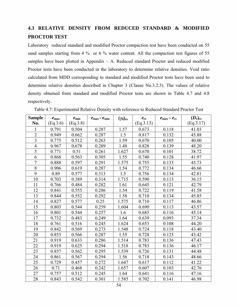
54

4.3 RELATIVE DENSITY FROM REDUCED STANDARD & MODIFIED

PROCTOR TEST

Laboratory reduced standard and modified Proctor compaction test have been conducted on 55

sand samples starting from 4 % or 6 % water content. All the compaction test figures of 55

samples have been plotted in Appendix – A. Reduced standard Proctor and reduced modified

Proctor tests have been conducted in the laboratory to determine relative densities. Void ratio

calculated from MDD corresponding to standard and modified Proctor tests have been used to

determine relative densities described in Chapter 3 (Clause No.3.2.5). The values of relative

density obtained from standard and modified Proctor tests are shown in Table 4.7 and 4.8

respectively.

Table 4.7: Experimental Relative Density with reference to Reduced Standard Proctor Test

Sample No.

emax (Eq.3.6)

emin (Eq.3.8)

emax - emin (γd)rs ers (Eq.3.13)

emax – ers (Dr)rs (Eq.3.17)

1 0.791 0.504 0.287 1.57 0.673 0.118 41.03 2 0.949 0.662 0.287 1.5 0.817 0.132 45.88 3 0.775 0.512 0.263 1.59 0.670 0.105 40.00 4 0.967 0.678 0.289 1.48 0.828 0.139 48.20 5 0.771 0.51 0.261 1.627 0.670 0.101 38.72 6 0.868 0.563 0.305 1.55 0.740 0.128 41.97 7 0.888 0.597 0.291 1.575 0.755 0.133 45.73 8 0.906 0.619 0.287 1.54 0.772 0.134 46.66 9 0.89 0.577 0.313 1.5 0.756 0.134 42.81 10 0.703 0.389 0.314 1.715 0.590 0.113 36.15 11 0.766 0.484 0.282 1.61 0.645 0.121 42.79 12 0.841 0.555 0.286 1.54 0.722 0.119 41.58 13 0.844 0.552 0.292 1.58 0.710 0.134 45.85 14 0.827 0.577 0.25 1.575 0.710 0.117 46.86 15 0.803 0.544 0.259 1.604 0.690 0.113 43.57 16 0.801 0.544 0.257 1.6 0.685 0.116 45.14 17 0.732 0.483 0.249 1.64 0.639 0.093 37.34 18 0.761 0.516 0.245 1.624 0.653 0.108 44.20 19 0.842 0.569 0.273 1.548 0.724 0.118 43.40 20 0.853 0.566 0.287 1.55 0.728 0.125 43.42 21 0.919 0.633 0.286 1.514 0.783 0.136 47.43 22 0.919 0.625 0.294 1.518 0.783 0.136 46.17 23 0.857 0.562 0.295 1.539 0.726 0.131 44.48 24 0.861 0.567 0.294 1.56 0.718 0.143 48.66 25 0.729 0.457 0.272 1.647 0.617 0.112 41.22 26 0.71 0.468 0.242 1.657 0.607 0.103 42.76 27 0.757 0.512 0.245 1.64 0.641 0.116 47.16 28 0.843 0.542 0.301 1.585 0.702 0.141 46.98

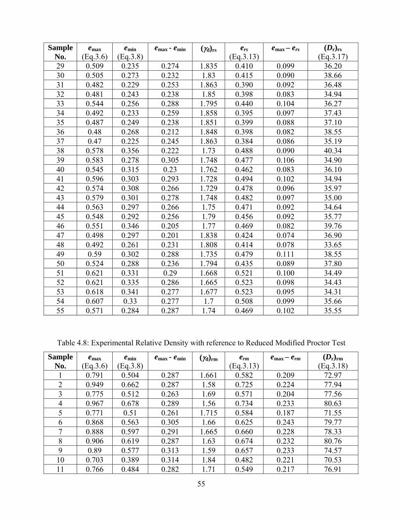
55

Sample No.

emax (Eq.3.6)

emin (Eq.3.8)

emax - emin (γd)rs ers (Eq.3.13)

emax – ers (Dr)rs (Eq.3.17)

29 0.509 0.235 0.274 1.835 0.410 0.099 36.20 30 0.505 0.273 0.232 1.83 0.415 0.090 38.66 31 0.482 0.229 0.253 1.863 0.390 0.092 36.48 32 0.481 0.243 0.238 1.85 0.398 0.083 34.94 33 0.544 0.256 0.288 1.795 0.440 0.104 36.27 34 0.492 0.233 0.259 1.858 0.395 0.097 37.43 35 0.487 0.249 0.238 1.851 0.399 0.088 37.10 36 0.48 0.268 0.212 1.848 0.398 0.082 38.55 37 0.47 0.225 0.245 1.863 0.384 0.086 35.19 38 0.578 0.356 0.222 1.73 0.488 0.090 40.34 39 0.583 0.278 0.305 1.748 0.477 0.106 34.90 40 0.545 0.315 0.23 1.762 0.462 0.083 36.10 41 0.596 0.303 0.293 1.728 0.494 0.102 34.94 42 0.574 0.308 0.266 1.729 0.478 0.096 35.97 43 0.579 0.301 0.278 1.748 0.482 0.097 35.00 44 0.563 0.297 0.266 1.75 0.471 0.092 34.64 45 0.548 0.292 0.256 1.79 0.456 0.092 35.77 46 0.551 0.346 0.205 1.77 0.469 0.082 39.76 47 0.498 0.297 0.201 1.838 0.424 0.074 36.90 48 0.492 0.261 0.231 1.808 0.414 0.078 33.65 49 0.59 0.302 0.288 1.735 0.479 0.111 38.55 50 0.524 0.288 0.236 1.794 0.435 0.089 37.80 51 0.621 0.331 0.29 1.668 0.521 0.100 34.49 52 0.621 0.335 0.286 1.665 0.523 0.098 34.43 53 0.618 0.341 0.277 1.677 0.523 0.095 34.31 54 0.607 0.33 0.277 1.7 0.508 0.099 35.66 55 0.571 0.284 0.287 1.74 0.469 0.102 35.55

Table 4.8: Experimental Relative Density with reference to Reduced Modified Proctor Test

Sample No.

emax (Eq.3.6)

emin (Eq.3.8)

emax - emin (γd)rm erm (Eq.3.13)

emax – erm (Dr)rm (Eq.3.18)

1 0.791 0.504 0.287 1.661 0.582 0.209 72.97 2 0.949 0.662 0.287 1.58 0.725 0.224 77.94 3 0.775 0.512 0.263 1.69 0.571 0.204 77.56 4 0.967 0.678 0.289 1.56 0.734 0.233 80.63 5 0.771 0.51 0.261 1.715 0.584 0.187 71.55 6 0.868 0.563 0.305 1.66 0.625 0.243 79.77 7 0.888 0.597 0.291 1.665 0.660 0.228 78.33 8 0.906 0.619 0.287 1.63 0.674 0.232 80.76 9 0.89 0.577 0.313 1.59 0.657 0.233 74.57 10 0.703 0.389 0.314 1.84 0.482 0.221 70.53 11 0.766 0.484 0.282 1.71 0.549 0.217 76.91

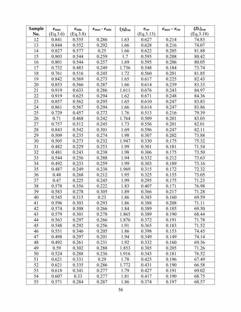
56

Sample No.

emax (Eq.3.6)

emin (Eq.3.8)

emax - emin (γd)rm erm (Eq.3.13)

emax – erm (Dr)rm (Eq.3.18)

12 0.841 0.555 0.286 1.63 0.627 0.214 74.83 13 0.844 0.552 0.292 1.66 0.628 0.216 74.07 14 0.827 0.577 0.25 1.66 0.622 0.205 81.88 15 0.803 0.544 0.259 1.7 0.595 0.208 80.42 16 0.801 0.544 0.257 1.69 0.595 0.206 80.05 17 0.732 0.483 0.249 1.736 0.548 0.184 73.74 18 0.761 0.516 0.245 1.72 0.560 0.201 81.85 19 0.842 0.569 0.273 1.65 0.617 0.225 82.43 20 0.853 0.566 0.287 1.66 0.614 0.239 83.33 21 0.919 0.633 0.286 1.611 0.676 0.243 84.97 22 0.919 0.625 0.294 1.62 0.671 0.248 84.36 23 0.857 0.562 0.295 1.65 0.610 0.247 83.83 24 0.861 0.567 0.294 1.66 0.614 0.247 83.86 25 0.729 0.457 0.272 1.76 0.513 0.216 79.39 26 0.71 0.468 0.242 1.764 0.509 0.201 83.03 27 0.757 0.512 0.245 1.73 0.556 0.201 82.01 28 0.843 0.542 0.301 1.69 0.596 0.247 82.11 29 0.509 0.235 0.274 1.98 0.307 0.202 73.88 30 0.505 0.273 0.232 1.947 0.330 0.175 75.32 31 0.482 0.229 0.253 1.99 0.301 0.181 71.54 32 0.481 0.243 0.238 1.98 0.306 0.175 73.50 33 0.544 0.256 0.288 1.94 0.332 0.212 73.63 34 0.492 0.233 0.259 1.99 0.303 0.189 73.16 35 0.487 0.249 0.238 1.969 0.315 0.172 72.32 36 0.48 0.268 0.212 1.95 0.325 0.155 73.05 37 0.47 0.225 0.245 1.99 0.295 0.175 71.23 38 0.578 0.356 0.222 1.83 0.407 0.171 76.98 39 0.583 0.278 0.305 1.89 0.366 0.217 71.28 40 0.545 0.315 0.23 1.86 0.385 0.160 69.59 41 0.596 0.303 0.293 1.86 0.388 0.208 71.11 42 0.574 0.308 0.266 1.84 0.389 0.185 69.50 43 0.579 0.301 0.278 1.865 0.389 0.190 68.44 44 0.563 0.297 0.266 1.876 0.372 0.191 71.78 45 0.548 0.292 0.256 1.91 0.365 0.183 71.52 46 0.551 0.346 0.205 1.86 0.398 0.153 74.45 47 0.498 0.297 0.201 1.94 0.349 0.149 74.14 48 0.492 0.261 0.231 1.92 0.332 0.160 69.36 49 0.59 0.302 0.288 1.853 0.385 0.205 71.26 50 0.524 0.288 0.236 1.916 0.343 0.181 76.52 51 0.621 0.331 0.29 1.78 0.425 0.196 67.49 52 0.621 0.335 0.286 1.772 0.431 0.190 66.58 53 0.618 0.341 0.277 1.79 0.427 0.191 69.02 54 0.607 0.33 0.277 1.81 0.417 0.190 68.75 55 0.571 0.284 0.287 1.86 0.374 0.197 68.57

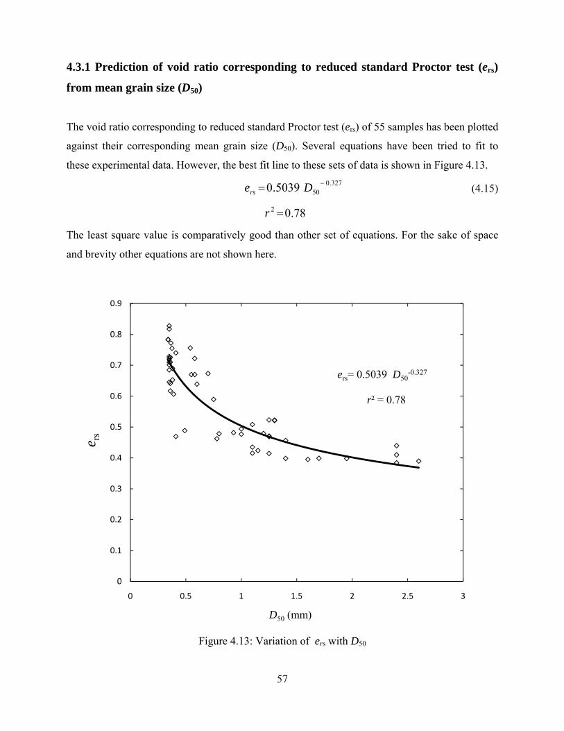
57

4.3.1 Prediction of void ratio corresponding to reduced standard Proctor test (ers)

from mean grain size (D50)

The void ratio corresponding to reduced standard Proctor test (ers) of 55 samples has been plotted

against their corresponding mean grain size (D50). Several equations have been tried to fit to

these experimental data. However, the best fit line to these sets of data is shown in Figure 4.13. 327.0

505039.0 −= Ders

(4.15)

78.02 =r

The least square value is comparatively good than other set of equations. For the sake of space

and brevity other equations are not shown here.

Figure 4.13: Variation of ers with D50

ers= 0.5039 D50-0.327

r² = 0.78

0

0.1

0.2

0.3

0.4

0.5

0.6

0.7

0.8

0.9

0 0.5 1 1.5 2 2.5 3

e rs

D50 (mm)

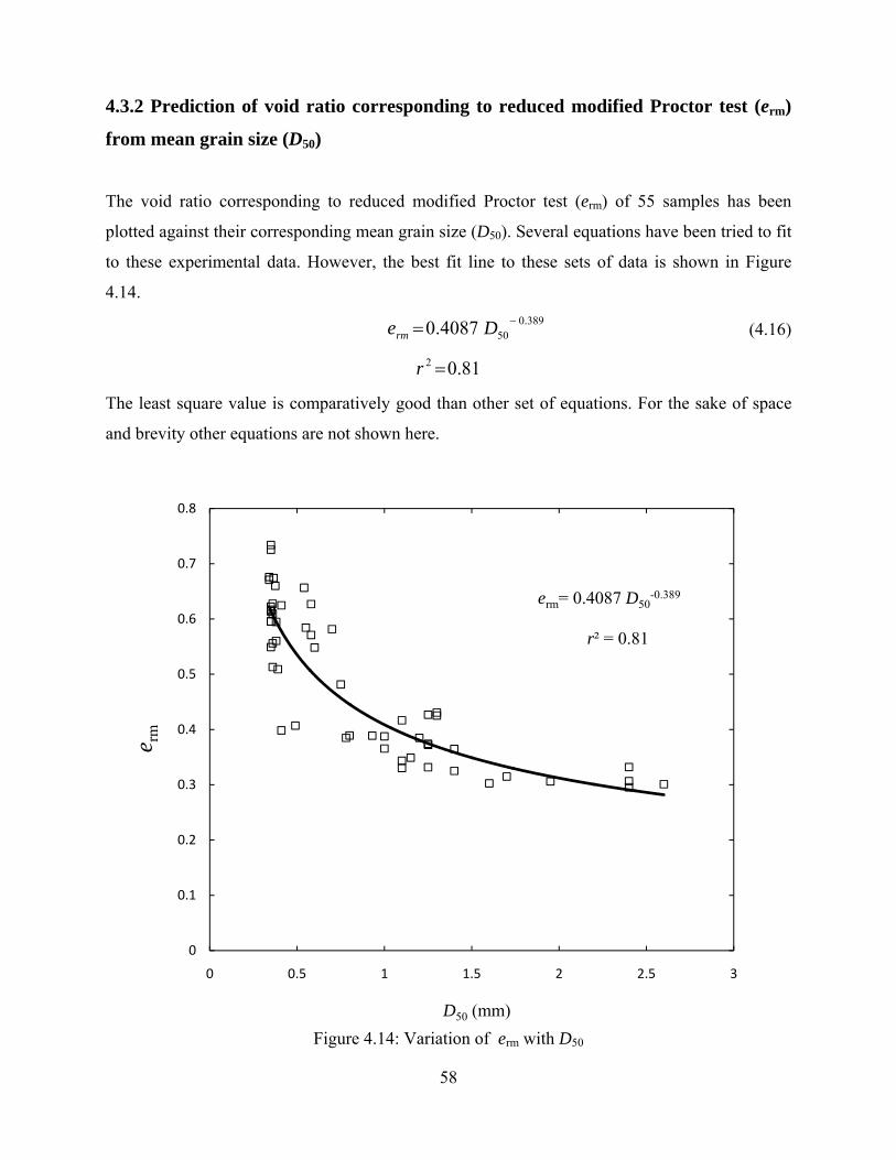
58

4.3.2 Prediction of void ratio corresponding to reduced modified Proctor test (erm)

from mean grain size (D50)

The void ratio corresponding to reduced modified Proctor test (erm) of 55 samples has been

plotted against their corresponding mean grain size (D50). Several equations have been tried to fit

to these experimental data. However, the best fit line to these sets of data is shown in Figure

4.14. 389.0

504087.0 −= Derm

(4.16)

81.02 =r

The least square value is comparatively good than other set of equations. For the sake of space

and brevity other equations are not shown here.

Figure 4.14: Variation of erm with D50

erm= 0.4087 D50-0.389

r² = 0.81

0

0.1

0.2

0.3

0.4

0.5

0.6

0.7

0.8

0 0.5 1 1.5 2 2.5 3

e rm

D50 (mm)

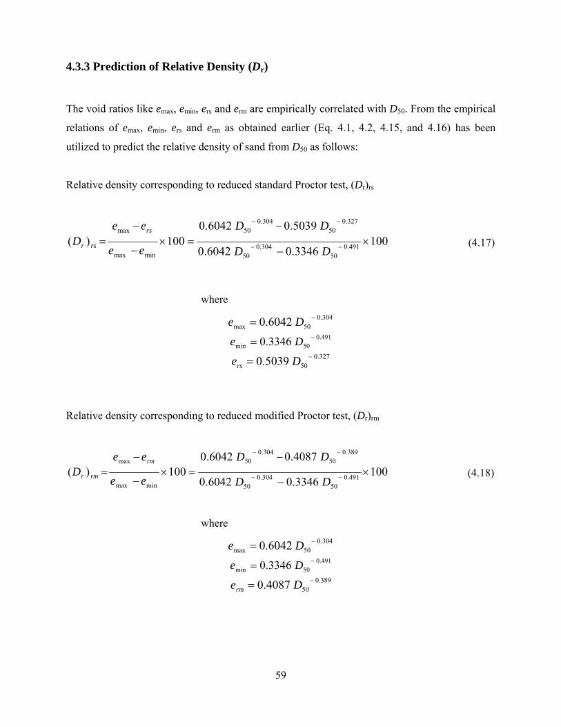
59

4.3.3 Prediction of Relative Density (Dr)

The void ratios like emax, emin, ers and erm are empirically correlated with D50. From the empirical

relations of emax, emin, ers and erm as obtained earlier (Eq. 4.1, 4.2, 4.15, and 4.16) has been

utilized to predict the relative density of sand from D50 as follows:

Relative density corresponding to reduced standard Proctor test, (Dr)rs

1003346.06042.0

5039.06042.0100)( 491.0

50304.0

50

327.050

304.050

minmax

max

×−

−=×

−

−= −−

−−

DD

DD

ee

eeD

rs

rsr

(4.17)

where 304.0

50max 6042.0 −= De 491.0

50min 3346.0 −= De 327.0

505039.0 −= Ders

Relative density corresponding to reduced modified Proctor test, (Dr)rm

1003346.06042.0

4087.06042.0100)( 491.0

50304.0

50

389.050

304.050

minmax

max

×−

−=×

−

−= −−

−−

DD

DD

ee

eeD

rm

rmr

(4.18)

where 304.0

50max 6042.0 −= De 491.0

50min 3346.0 −= De 389.0

504087.0 −= Derm

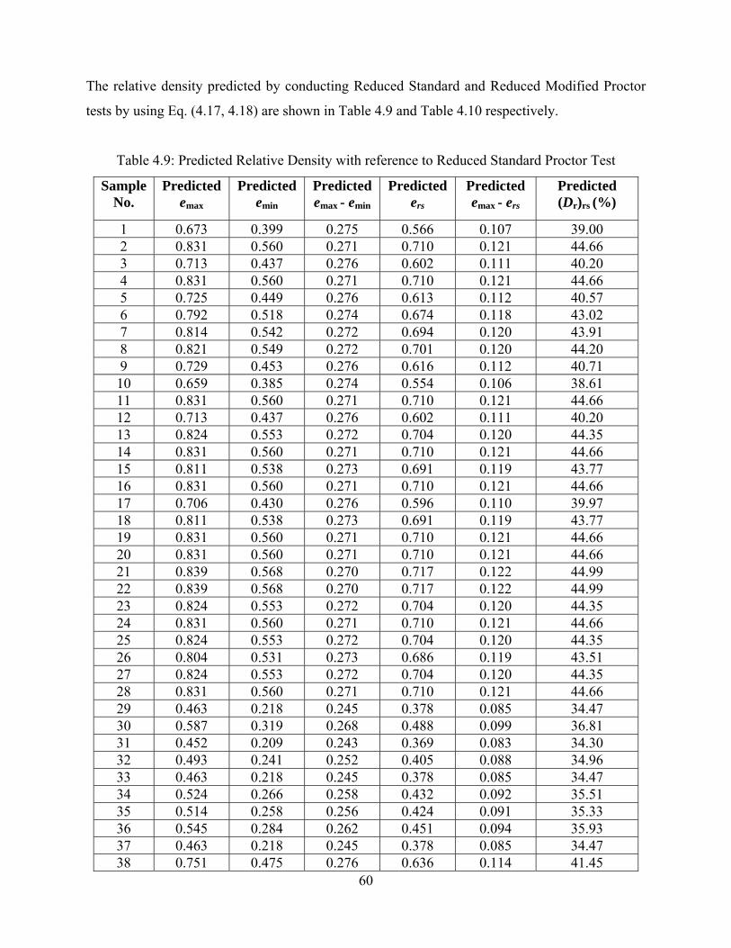
60

The relative density predicted by conducting Reduced Standard and Reduced Modified Proctor

tests by using Eq. (4.17, 4.18) are shown in Table 4.9 and Table 4.10 respectively.

Table 4.9: Predicted Relative Density with reference to Reduced Standard Proctor Test

Sample No.

Predicted emax

Predicted emin

Predicted emax - emin

Predicted ers

Predicted emax - ers

Predicted (Dr)rs (%)

1 0.673 0.399 0.275 0.566 0.107 39.00 2 0.831 0.560 0.271 0.710 0.121 44.66 3 0.713 0.437 0.276 0.602 0.111 40.20 4 0.831 0.560 0.271 0.710 0.121 44.66 5 0.725 0.449 0.276 0.613 0.112 40.57 6 0.792 0.518 0.274 0.674 0.118 43.02 7 0.814 0.542 0.272 0.694 0.120 43.91 8 0.821 0.549 0.272 0.701 0.120 44.20 9 0.729 0.453 0.276 0.616 0.112 40.71 10 0.659 0.385 0.274 0.554 0.106 38.61 11 0.831 0.560 0.271 0.710 0.121 44.66 12 0.713 0.437 0.276 0.602 0.111 40.20 13 0.824 0.553 0.272 0.704 0.120 44.35 14 0.831 0.560 0.271 0.710 0.121 44.66 15 0.811 0.538 0.273 0.691 0.119 43.77 16 0.831 0.560 0.271 0.710 0.121 44.66 17 0.706 0.430 0.276 0.596 0.110 39.97 18 0.811 0.538 0.273 0.691 0.119 43.77 19 0.831 0.560 0.271 0.710 0.121 44.66 20 0.831 0.560 0.271 0.710 0.121 44.66 21 0.839 0.568 0.270 0.717 0.122 44.99 22 0.839 0.568 0.270 0.717 0.122 44.99 23 0.824 0.553 0.272 0.704 0.120 44.35 24 0.831 0.560 0.271 0.710 0.121 44.66 25 0.824 0.553 0.272 0.704 0.120 44.35 26 0.804 0.531 0.273 0.686 0.119 43.51 27 0.824 0.553 0.272 0.704 0.120 44.35 28 0.831 0.560 0.271 0.710 0.121 44.66 29 0.463 0.218 0.245 0.378 0.085 34.47 30 0.587 0.319 0.268 0.488 0.099 36.81 31 0.452 0.209 0.243 0.369 0.083 34.30 32 0.493 0.241 0.252 0.405 0.088 34.96 33 0.463 0.218 0.245 0.378 0.085 34.47 34 0.524 0.266 0.258 0.432 0.092 35.51 35 0.514 0.258 0.256 0.424 0.091 35.33 36 0.545 0.284 0.262 0.451 0.094 35.93 37 0.463 0.218 0.245 0.378 0.085 34.47 38 0.751 0.475 0.276 0.636 0.114 41.45

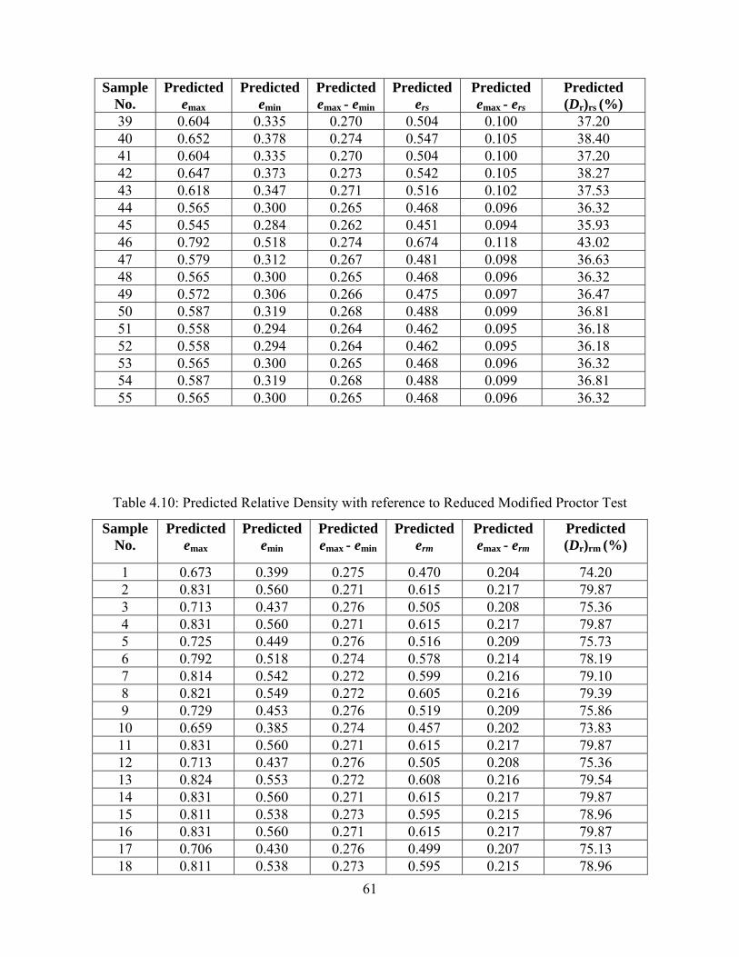
61

Sample No.

Predicted emax

Predicted emin

Predicted emax - emin

Predicted ers

Predicted emax - ers

Predicted (Dr)rs (%)

39 0.604 0.335 0.270 0.504 0.100 37.20 40 0.652 0.378 0.274 0.547 0.105 38.40 41 0.604 0.335 0.270 0.504 0.100 37.20 42 0.647 0.373 0.273 0.542 0.105 38.27 43 0.618 0.347 0.271 0.516 0.102 37.53 44 0.565 0.300 0.265 0.468 0.096 36.32 45 0.545 0.284 0.262 0.451 0.094 35.93 46 0.792 0.518 0.274 0.674 0.118 43.02 47 0.579 0.312 0.267 0.481 0.098 36.63 48 0.565 0.300 0.265 0.468 0.096 36.32 49 0.572 0.306 0.266 0.475 0.097 36.47 50 0.587 0.319 0.268 0.488 0.099 36.81 51 0.558 0.294 0.264 0.462 0.095 36.18 52 0.558 0.294 0.264 0.462 0.095 36.18 53 0.565 0.300 0.265 0.468 0.096 36.32 54 0.587 0.319 0.268 0.488 0.099 36.81 55 0.565 0.300 0.265 0.468 0.096 36.32

Table 4.10: Predicted Relative Density with reference to Reduced Modified Proctor Test

Sample No.

Predicted emax

Predicted emin

Predicted emax - emin

Predicted erm

Predicted emax - erm

Predicted (Dr)rm (%)

1 0.673 0.399 0.275 0.470 0.204 74.20 2 0.831 0.560 0.271 0.615 0.217 79.87 3 0.713 0.437 0.276 0.505 0.208 75.36 4 0.831 0.560 0.271 0.615 0.217 79.87 5 0.725 0.449 0.276 0.516 0.209 75.73 6 0.792 0.518 0.274 0.578 0.214 78.19 7 0.814 0.542 0.272 0.599 0.216 79.10 8 0.821 0.549 0.272 0.605 0.216 79.39 9 0.729 0.453 0.276 0.519 0.209 75.86 10 0.659 0.385 0.274 0.457 0.202 73.83 11 0.831 0.560 0.271 0.615 0.217 79.87 12 0.713 0.437 0.276 0.505 0.208 75.36 13 0.824 0.553 0.272 0.608 0.216 79.54 14 0.831 0.560 0.271 0.615 0.217 79.87 15 0.811 0.538 0.273 0.595 0.215 78.96 16 0.831 0.560 0.271 0.615 0.217 79.87 17 0.706 0.430 0.276 0.499 0.207 75.13 18 0.811 0.538 0.273 0.595 0.215 78.96

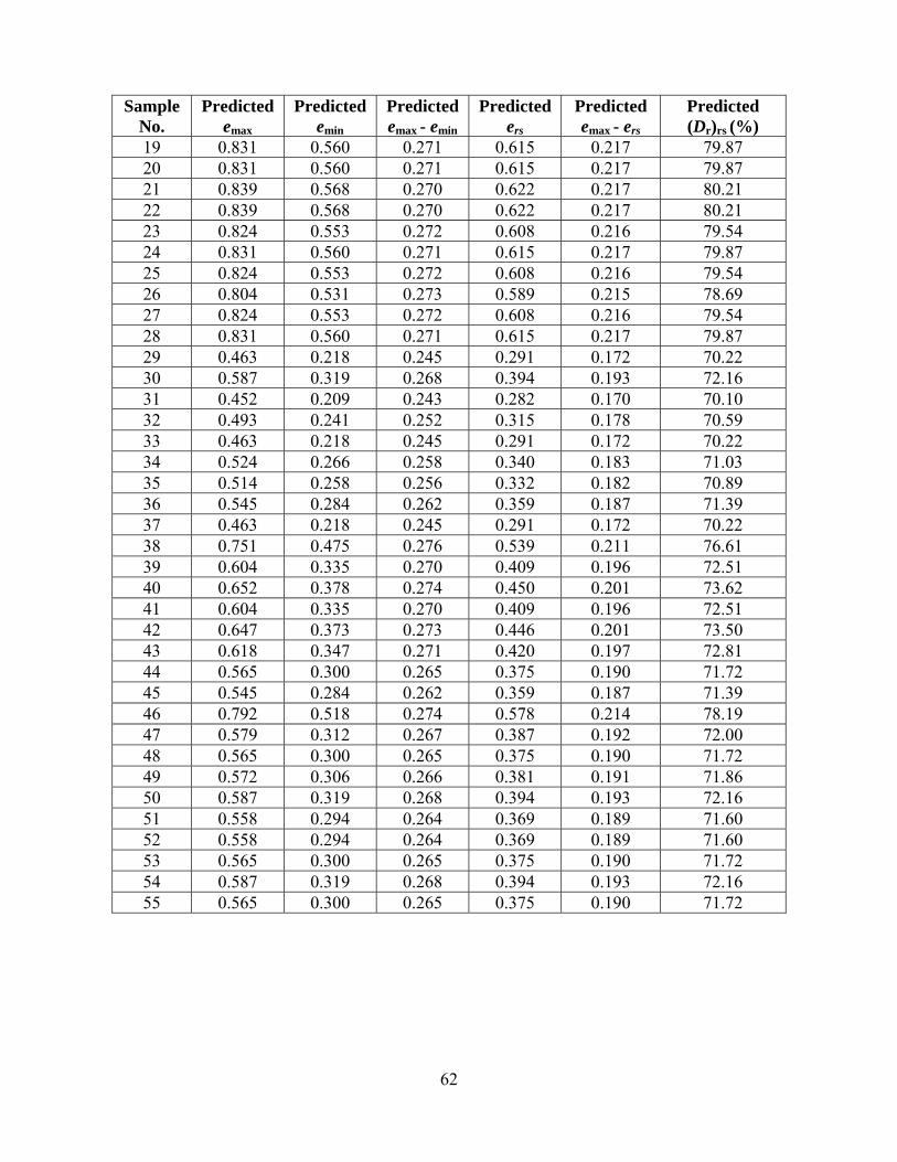
62

Sample No.

Predicted emax

Predicted emin

Predicted emax - emin

Predicted ers

Predicted emax - ers

Predicted (Dr)rs (%)

19 0.831 0.560 0.271 0.615 0.217 79.87 20 0.831 0.560 0.271 0.615 0.217 79.87 21 0.839 0.568 0.270 0.622 0.217 80.21 22 0.839 0.568 0.270 0.622 0.217 80.21 23 0.824 0.553 0.272 0.608 0.216 79.54 24 0.831 0.560 0.271 0.615 0.217 79.87 25 0.824 0.553 0.272 0.608 0.216 79.54 26 0.804 0.531 0.273 0.589 0.215 78.69 27 0.824 0.553 0.272 0.608 0.216 79.54 28 0.831 0.560 0.271 0.615 0.217 79.87 29 0.463 0.218 0.245 0.291 0.172 70.22 30 0.587 0.319 0.268 0.394 0.193 72.16 31 0.452 0.209 0.243 0.282 0.170 70.10 32 0.493 0.241 0.252 0.315 0.178 70.59 33 0.463 0.218 0.245 0.291 0.172 70.22 34 0.524 0.266 0.258 0.340 0.183 71.03 35 0.514 0.258 0.256 0.332 0.182 70.89 36 0.545 0.284 0.262 0.359 0.187 71.39 37 0.463 0.218 0.245 0.291 0.172 70.22 38 0.751 0.475 0.276 0.539 0.211 76.61 39 0.604 0.335 0.270 0.409 0.196 72.51 40 0.652 0.378 0.274 0.450 0.201 73.62 41 0.604 0.335 0.270 0.409 0.196 72.51 42 0.647 0.373 0.273 0.446 0.201 73.50 43 0.618 0.347 0.271 0.420 0.197 72.81 44 0.565 0.300 0.265 0.375 0.190 71.72 45 0.545 0.284 0.262 0.359 0.187 71.39 46 0.792 0.518 0.274 0.578 0.214 78.19 47 0.579 0.312 0.267 0.387 0.192 72.00 48 0.565 0.300 0.265 0.375 0.190 71.72 49 0.572 0.306 0.266 0.381 0.191 71.86 50 0.587 0.319 0.268 0.394 0.193 72.16 51 0.558 0.294 0.264 0.369 0.189 71.60 52 0.558 0.294 0.264 0.369 0.189 71.60 53 0.565 0.300 0.265 0.375 0.190 71.72 54 0.587 0.319 0.268 0.394 0.193 72.16 55 0.565 0.300 0.265 0.375 0.190 71.72

63

4.3.4 Comparison of predicted relative density with experimental values

The values of relative density obtained from the experimental Reduced Standard and Reduced

Modified Proctor tests have been plotted against the predicted values obtained as a function of

D50 are shown in Figure 4.15. The same has been presented in Table 4.11 for better comparison.

Figure 4.15: Plot of Dr (experimental) versus Dr (predicted)

30

35

40

45

50

55

60

65

70

75

80

85

90

30 35 40 45 50 55 60 65 70 75 80 85 90

Dr(P

redi

cted

)

Dr (Experimental)

Reduced modified proctor

Reduced Standard proctor

Line of equality

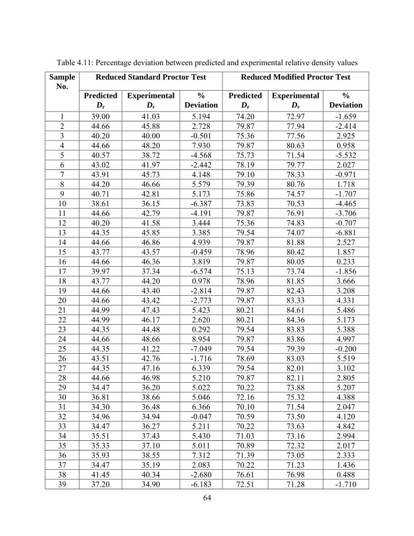
64

Table 4.11: Percentage deviation between predicted and experimental relative density values

Sample No.

Reduced Standard Proctor Test Reduced Modified Proctor Test

Predicted Dr

Experimental Dr

% Deviation

Predicted Dr

Experimental Dr

% Deviation

1 39.00 41.03 5.194 74.20 72.97 -1.659 2 44.66 45.88 2.728 79.87 77.94 -2.414 3 40.20 40.00 -0.501 75.36 77.56 2.925 4 44.66 48.20 7.930 79.87 80.63 0.958 5 40.57 38.72 -4.568 75.73 71.54 -5.532 6 43.02 41.97 -2.442 78.19 79.77 2.027 7 43.91 45.73 4.148 79.10 78.33 -0.971 8 44.20 46.66 5.579 79.39 80.76 1.718 9 40.71 42.81 5.173 75.86 74.57 -1.707 10 38.61 36.15 -6.387 73.83 70.53 -4.465 11 44.66 42.79 -4.191 79.87 76.91 -3.706 12 40.20 41.58 3.444 75.36 74.83 -0.707 13 44.35 45.85 3.385 79.54 74.07 -6.881 14 44.66 46.86 4.939 79.87 81.88 2.527 15 43.77 43.57 -0.459 78.96 80.42 1.857 16 44.66 46.36 3.819 79.87 80.05 0.233 17 39.97 37.34 -6.574 75.13 73.74 -1.856 18 43.77 44.20 0.978 78.96 81.85 3.666 19 44.66 43.40 -2.814 79.87 82.43 3.208 20 44.66 43.42 -2.773 79.87 83.33 4.331 21 44.99 47.43 5.423 80.21 84.61 5.486 22 44.99 46.17 2.620 80.21 84.36 5.173 23 44.35 44.48 0.292 79.54 83.83 5.388 24 44.66 48.66 8.954 79.87 83.86 4.997 25 44.35 41.22 -7.049 79.54 79.39 -0.200 26 43.51 42.76 -1.716 78.69 83.03 5.519 27 44.35 47.16 6.339 79.54 82.01 3.102 28 44.66 46.98 5.210 79.87 82.11 2.805 29 34.47 36.20 5.022 70.22 73.88 5.207 30 36.81 38.66 5.046 72.16 75.32 4.388 31 34.30 36.48 6.366 70.10 71.54 2.047 32 34.96 34.94 -0.047 70.59 73.50 4.120 33 34.47 36.27 5.211 70.22 73.63 4.842 34 35.51 37.43 5.430 71.03 73.16 2.994 35 35.33 37.10 5.011 70.89 72.32 2.017 36 35.93 38.55 7.312 71.39 73.05 2.333 37 34.47 35.19 2.083 70.22 71.23 1.436 38 41.45 40.34 -2.680 76.61 76.98 0.488 39 37.20 34.90 -6.183 72.51 71.28 -1.710

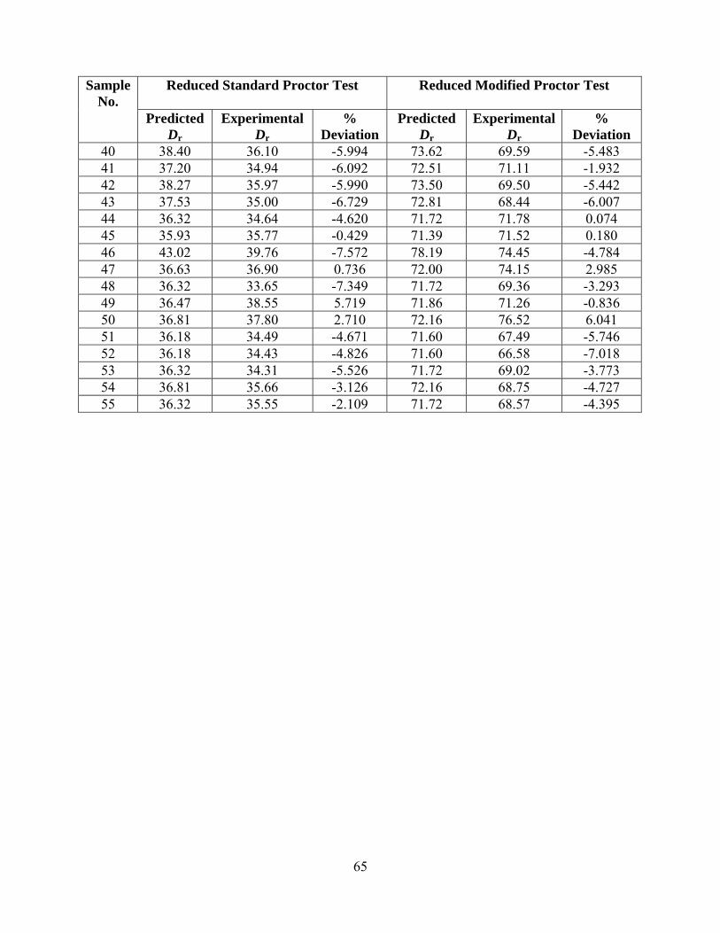
65

Sample No.

Reduced Standard Proctor Test

Reduced Modified Proctor Test

Predicted Dr

Experimental Dr

% Deviation

Predicted Dr

Experimental Dr

% Deviation

40 38.40 36.10 -5.994 73.62 69.59 -5.483 41 37.20 34.94 -6.092 72.51 71.11 -1.932 42 38.27 35.97 -5.990 73.50 69.50 -5.442 43 37.53 35.00 -6.729 72.81 68.44 -6.007 44 36.32 34.64 -4.620 71.72 71.78 0.074 45 35.93 35.77 -0.429 71.39 71.52 0.180 46 43.02 39.76 -7.572 78.19 74.45 -4.784 47 36.63 36.90 0.736 72.00 74.15 2.985 48 36.32 33.65 -7.349 71.72 69.36 -3.293 49 36.47 38.55 5.719 71.86 71.26 -0.836 50 36.81 37.80 2.710 72.16 76.52 6.041 51 36.18 34.49 -4.671 71.60 67.49 -5.746 52 36.18 34.43 -4.826 71.60 66.58 -7.018 53 36.32 34.31 -5.526 71.72 69.02 -3.773 54 36.81 35.66 -3.126 72.16 68.75 -4.727 55 36.32 35.55 -2.109 71.72 68.57 -4.395

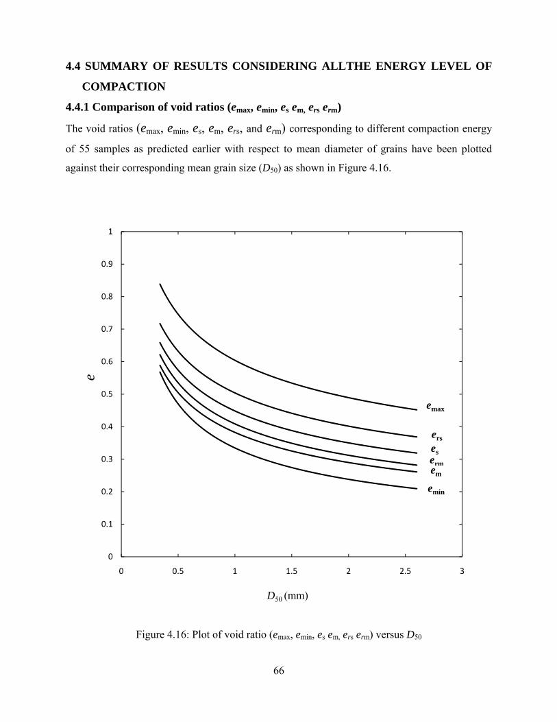
66

4.4 SUMMARY OF RESULTS CONSIDERING ALLTHE ENERGY LEVEL OF

COMPACTION

4.4.1 Comparison of void ratios (emax, emin, es em, ers erm)

The void ratios (emax, emin, es, em, ers, and erm) corresponding to different compaction energy

of 55 samples as predicted earlier with respect to mean diameter of grains have been plotted

against their corresponding mean grain size (D50) as shown in Figure 4.16.

Figure 4.16: Plot of void ratio (emax, emin, es em, ers erm) versus D50

0

0.1

0.2

0.3

0.4

0.5

0.6

0.7

0.8

0.9

1

0 0.5 1 1.5 2 2.5 3

e

D50 (mm)

emax

emin

ersesermem

67

4.4.2 Empirical equations for void ratios (emax, emin, es em, ers erm) at particular energy

levels

Based on the test results, correlation of voids ratio (e), compaction energy (E) and mean grain

size (D50) have been made. The equation for the void ratios at six energy levels of compaction (E)

done in the laboratory i.e. 356 kNm/m3, 593 kN-m/m3, 1295 kN-m/m3, 2698 kN-m/m3 loosest

state, and densest state can be expressed in the form as below:

bDae −= 50 (4.19)

where, e = void ratio at a particular energy level

a = a constant for a particular energy level

b = a constant for a particular energy level

The values of coefficient “a” and “b” have been presented in Table 4.12 for different energy

levels under consideration. At any particular energy level under consideration, the void ratio can

be correlated with the mean diameter of grains by the equation 4.19 and Table 4.12.

Table 4.12: Coefficient “a” and “b” values for different energy levels

Energy Level Void ratio a b

Minimum emax 0.6042 0.304

356 kN-m/m3 ers 0.5039 0.327

593 kN-m/m3 es 0.4484 0.356

1295 kN-m/m3 erm 0.4087 0.389

2698 kN-m/m3 em 0.3825 0.400

Maximum emin 0.3346 0.491

The empirical equations developed for a particular energy level are as follows.

304.0

50max 6042.0 −= De 76.02 =r (4.20)

327.0

505039.0 −= Ders 78.02 =r (4.21)

68

356.0

504484.0 −= Des 80.02 =r (4.22)

389.0

504087.0 −= Derm 81.02 =r (4.23)

4.0

503825.0 −= Dem 81.02 =r (4.24)

491.0

50min 3346.0 −= De 85.02 =r (4.25)

4.4.3 Empirical equations for relative density (Dr) at particular energy levels

The relative density at particular energy of compaction such as reduced standard, standard,

reduced modified and modified compaction can be correlated with a single parameter like the

mean diameter of grains by the following equations:

Relative density for 356 kN-m/m3 energy level

1003346.06042.0

5039.06042.0100)( 491.0

50304.0

50

327.050

304.050

minmax

max

×−

−=×

−

−= −−

−−

DD

DD

ee

eeD

rs

rsr

(4.26)

Relative density for 593 kN-m/m3 energy level

1003346.06042.0

4484.06042.0100)( 491.0

50304.0

50

356.050

304.050

minmax

max

×−

−=×

−

−= −−

−−

DD

DD

ee

eeD

s

sr

(4.27)

Relative density for 1295 kN-m/m3 energy level

1003346.06042.0

4087.06042.0100)( 491.0

50304.0

50

389.050

304.050

minmax

max

×−

−=×

−

−= −−

−−

DD

DD

ee

eeD

rm

rmr

(4.28)

Relative density for 2698 kN-m/m3 energy level

100

3346.06042.0

3825.06042.0100)( 491.0

50304.0

50

4.050

304.050

minmax

max

×−

−=×

−

−= −−

−−

DD

DD

ee

eeD

m

mr

(4.29)

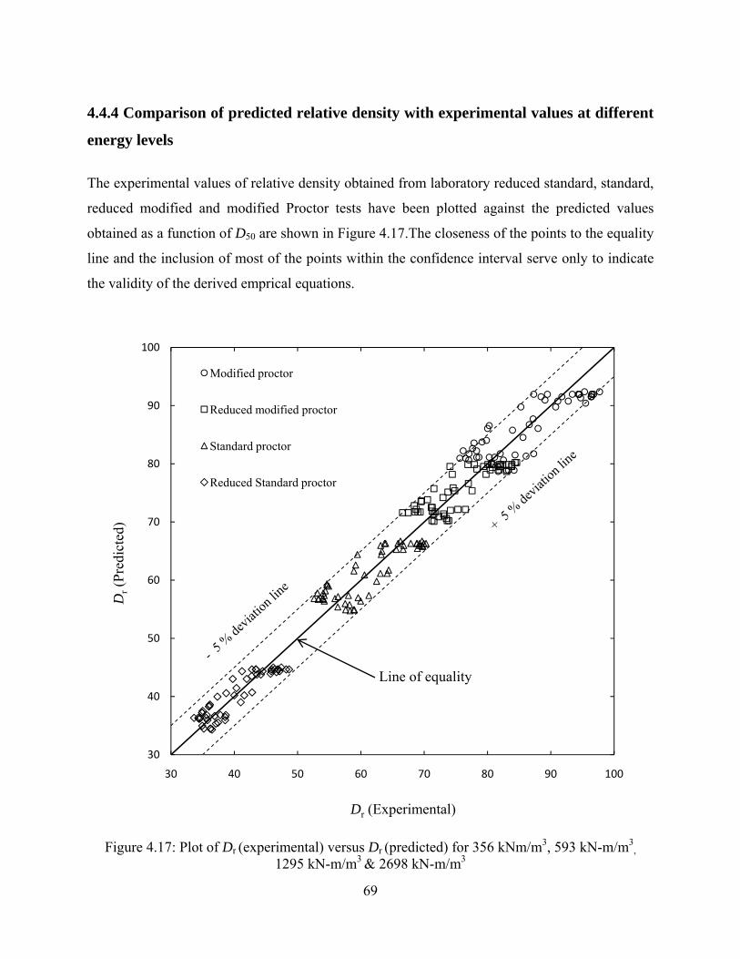
69

4.4.4 Comparison of predicted relative density with experimental values at different

energy levels

The experimental values of relative density obtained from laboratory reduced standard, standard,

reduced modified and modified Proctor tests have been plotted against the predicted values

obtained as a function of D50 are shown in Figure 4.17.The closeness of the points to the equality

line and the inclusion of most of the points within the confidence interval serve only to indicate

the validity of the derived emprical equations.

Figure 4.17: Plot of Dr (experimental) versus Dr (predicted) for 356 kNm/m3, 593 kN-m/m3

, 1295 kN-m/m3 & 2698 kN-m/m3

30

40

50

60

70

80

90

100

30 40 50 60 70 80 90 100

Dr(P

redi

cted

)

Dr (Experimental)

Modified proctor

Reduced modified proctor

Standard proctor

Reduced Standard proctor

Line of equality

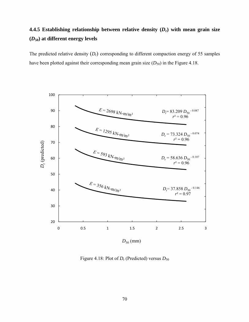
70

4.4.5 Establishing relationship between relative density (Dr) with mean grain size

(D50) at different energy levels

The predicted relative density (Dr) corresponding to different compaction energy of 55 samples

have been plotted against their corresponding mean grain size (D50) in the Figure 4.18.

Figure 4.18: Plot of Dr (Predicted) versus D50

Dr = 73.324 D50 - 0.074

r² = 0.96

Dr = 58.636 D50 - 0.107

r² = 0.96

Dr= 37.858 D50 - 0.146

r² = 0.97

Dr= 83.209 D50 - 0.087

r² = 0.96

20

30

40

50

60

70

80

90

100

0 0.5 1 1.5 2 2.5 3

Dr(p

redi

cted

)

D50 (mm)

71

The final best-fit models obtained is,

(4.30)

where Dr= relative density at a particular energy level

p = a constant for a particular energy level

q = a constant for a particular energy level

The values of coefficient “a” and “b” have been presented in Table 4.12 for different energy

levels.

Table 4.13: Coefficient “p” and “q” values for different energy levels

Energy Level p q

356 kN-m/m3 83.209 0.087

593 kN-m/m3 73.324 0.074

1295 kN-m/m3 58.636 0.107

2698 kN-m/m3 37.585 0.146

The empirical equations developed at particular compaction energy are,

087.0

50/356209.83)( 3

−

−= DD

mmkNr 96.02 =r (4.31)

074.0

50/593324.73)( 3

−

−= DD mmkNr 95.02 =r (4.32)

107.0

50/1295636.58)( 3

−

−= DD

mmkNr 96.02 =r (4.33)

146.0

50/2698 585.37)( 3−

−= DD mmkNr 97.02 =r (4.34)

qDpDr−= 50

0

CHAPTER 5

CONCLUSION

72

CONCLUSION

Laboratory test on 55 samples collected from river bed of Orissa have been carried out for

determining relative density at a particular compaction energy corresponding to the standard,

modified, reduced standard, reduced modified Proctor compaction tests. The void ratios at

different energy levels have been calculated from dry density obtained in the laboratory. From

the laboratory tests, the equations for void ratios at such particular energy levels have been

predicted by correlating with mean grain size. Relative densities at such energy levels have been

predicted by using the equations of void ratios which are function of mean grain size. The

following are generalized conclusions from the present work:

1. The most significant variable influencing void ratio is the mean grain size.

2. Predicted relative densities and experimental relative densities at particular energy level

are within + 5 %.

3. The relative densities at particular energy level can be correlated by empirical equations

in terms of mean grain size.

4. This will be helpful for the design specifications in the field since the relative density at

particular energy level is correlated with a single parameter such as mean grain size.

0

CHAPTER 6

SCOPE FOR FURTHER STUDY

73

SCOPE OF FURTHER STUDY

It is necessary to investigate the effect of angularity and particle shape on the maximum and

minimum void ratio and hence on the relative density of sand. It is recommended to derive

empirical equations of relative densities at any energy level of compaction. Correlation can be

done by considering both vibration as well as impact force while determining the relative density

in laboratory simulating to field conditions.

0

REFERENCES

74

REFERENCES

Abdel-Rahman, A. H. (2008). “Predicting compaction of cohesion less soils using ANN”,

Ground Improvement, Issue 161, pp. 3-8.

Aberg, B. (1992). “Void ratio of non cohesive soils and similar materials”, Journal of

Geotechnical Engineering, ASCE, Vol. 118, No. 9, pp. 1315-1334.

Aberg, B. (1996). “Grain-size distribution for smallest possible void ratio”, Journal of

Geotechnical Engineering, ASCE, Vol. 122, No. 1, pp. 74-77.

Aberg, B. (1996). “Void sizes in granular soils”, Journal of Geotechnical Engineering, ASCE,

Vol. 122, No. 3, pp. 236-239.

Arora, K. R. (2005). “Soil mechanics and foundation engineering”, Sixth edition, Standard

Publishers.

Barton, M. E., Cresswell, A., Brown, R. (2001). “Measuring the effect of mixed grading on the

maximum dry density of sands”, Geotechnical Testing Journal, ASTM, Vol. 24, No. 1, pp. 121-

127.

Burmister, D. M. (1948), “The Importance and Practical Use of Relative Density in Soil

Mechanics,” ASTM Proceedings, Presented at the Meeting of Committee D-18 on Soils for

Engineering Purposes held during the Fifty-first Annual Meeting, Detroit, Michigan, Vol. 48, pp.

1249–1268.

Cho, G. C., Dodds, J., Santamarina, J. C. (2006). “Particle Shape Effects on Packing Density,

Stiffness and Strength: Natural and Crushed Sands”, Journal of Geotechnical and

Geoenvironmental Engineering, ASCE, Vol. 132, No. 5, pp. 591-602.

Cubrinovski, M. and Ishihara, K. (2002). “Maximum and minimum void ratios characteristics of

sands”, Soils and Foundations, JGS, Vol. 42, No. 6, pp. 65-78.

75

D`Appolonia, D.J., Whitman, R.V., and D`Appolonia, E.D. (1969). “Sand Compaction with

Vibratory Rollers”, Journal of Soil Mechanics and Foundation Division, ASCE, Vol. 95, No.

SM 1, pp. 263-284.

Das, B. M. (2006). “Principles of geotechnical engineering”, Fifth edition,Thomson Brooks/cole.

Das, B. M. (2008). “Advanced soil mechanics”, Third edition, Taylor & Francis.

Dickin, E.A. (1973). “Influence of Grain Shape and Size upon the Limiting Porosities of Sands”,

ASTM STP 523, American Society for Testing and Materials, West Conshohocken, PA, pp.

113–120.

Gunaydın, O. (2008). “Estimation of Soil Compaction Parameters by using Statistical Analyses

and Artificial Neural Networks”, Journal of Environmental Geology, pp. 1-13.

Hatanaka, M and Feng, L. (2006). “Estimating Relative Density of Sandy soils”, Soils and

Foundations, JGS, Vol. 46, No. 3, pp. 299-313.

Hausmann M. R. (1990), “Engineering Principles of Ground Modification”, McGraw-Hill

Publishing Company, New York.

Hilf, J. (1956). “A Rapid Method of Compaction Control for embankments of Cohesive Soils”,

Engrg. Monograph, U. S. Bureau of Reclamation, Denver, Colo., (26), pp. 1-29. Holtz,W. G. (1973), “The Relative Density Approach-Uses, Testing Requirements, Reliability,

and Shortcomings,” Evaluation of Relative Density and its Role in Geotechnical Projects

Involving Cohesionless Soils, ASTM STP 523, American Society for Testing and Materials,

West Conshohocken, PA, pp. 5–17.

Holtz, R.D. and Kovacs, W.D. (1981). “An Introduction to Geotechnical Engineering”, Prentice-

Hall, Englewood Cliffs, N.J.

76

Holubec, I, D'Appolonia, E. (1973). “Effect of Particle Shape on the Engineering Properties of

Granular Soils”, ASTM, Digital Library / STP / STP523-EB / STP37879S.

IS: 2720 – Part III, (1980). “Determination of Specific Gravity”.

IS: 2720 – Part IV, (1985). “Grain Size Analysis”.

IS: 2720 – Part VII, (1980). “Determination of Water Content-Dry Density Relation using Light

Compaction”.

IS: 2720 – Part VIII, (1983). “Determination of Water Content-Dry Density Relation using

Heavy Compaction”.

IS: 2720 – Part XIV, (1983). “Determination of Density Index (Relative Density) of

Cohesionless Soil”.

Itabashi, K., Matsuo, M., Naito, M. and Kamiya, K. (2003). “Grain Shape Analysis and Packing

Property of Unified Coarse Granular Materials”, Soils and Foundations, JGS, Vol. 43, No. 1, pp.

115-127.

Johnson, A.W. and Sallberg, J. R. (1960). “Factors that Influence Field Compaction of Soils”,

Bulletin 272, Highway Research Board, pp. 206.

Johnston, M. M. (1973). “Laboratory Studies of Maximum and Minimum Dry Densities of

Cohesion less Soils”, ASTM, Digital Library / STP / STP523-EB / STP37869S.

Kokusho, T., Yoshida, Y. and Esashi, Y. (1983). “A Study on a Seismic Stability of Dense Sand

(Part 2), Evaluation method based on SPT N-value, Technical Report of Central research

Institute of Electric Power, (383026), pp. 1-32.

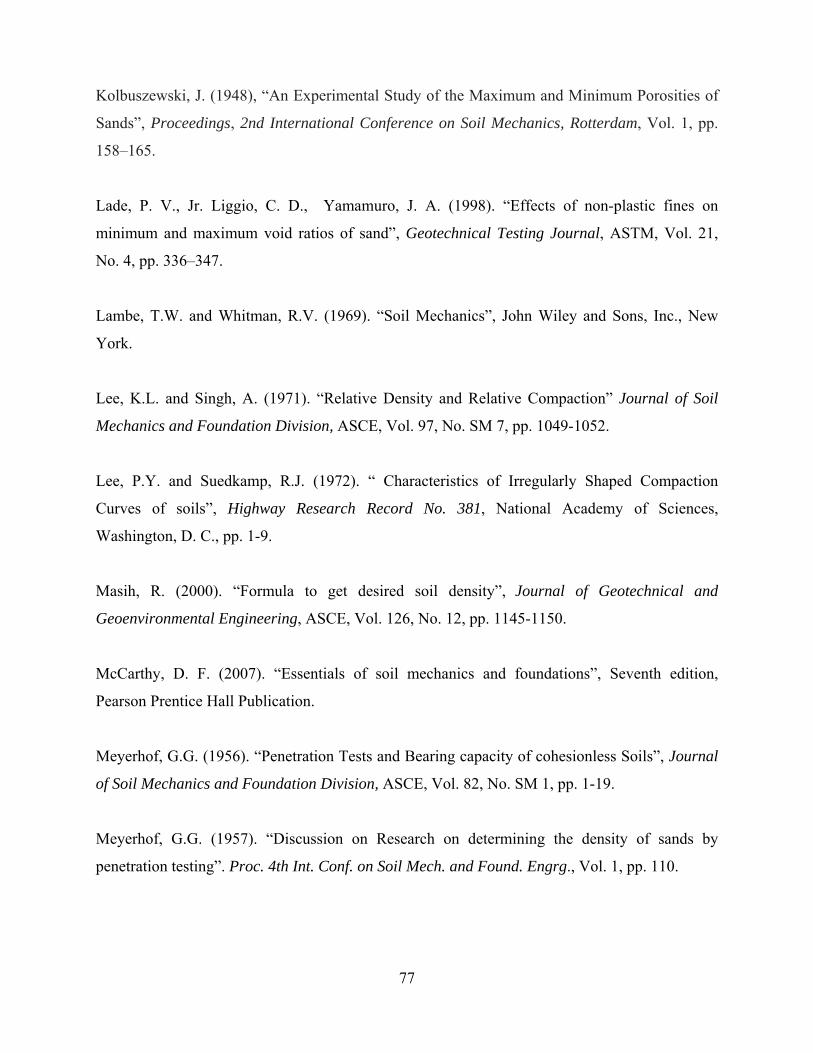
77

Kolbuszewski, J. (1948), “An Experimental Study of the Maximum and Minimum Porosities of

Sands”, Proceedings, 2nd International Conference on Soil Mechanics, Rotterdam, Vol. 1, pp.

158–165.

Lade, P. V., Jr. Liggio, C. D., Yamamuro, J. A. (1998). “Effects of non-plastic fines on

minimum and maximum void ratios of sand”, Geotechnical Testing Journal, ASTM, Vol. 21,

No. 4, pp. 336–347.

Lambe, T.W. and Whitman, R.V. (1969). “Soil Mechanics”, John Wiley and Sons, Inc., New

York.

Lee, K.L. and Singh, A. (1971). “Relative Density and Relative Compaction” Journal of Soil

Mechanics and Foundation Division, ASCE, Vol. 97, No. SM 7, pp. 1049-1052.

Lee, P.Y. and Suedkamp, R.J. (1972). “ Characteristics of Irregularly Shaped Compaction

Curves of soils”, Highway Research Record No. 381, National Academy of Sciences,

Washington, D. C., pp. 1-9.

Masih, R. (2000). “Formula to get desired soil density”, Journal of Geotechnical and

Geoenvironmental Engineering, ASCE, Vol. 126, No. 12, pp. 1145-1150.

McCarthy, D. F. (2007). “Essentials of soil mechanics and foundations”, Seventh edition,

Pearson Prentice Hall Publication.

Meyerhof, G.G. (1956). “Penetration Tests and Bearing capacity of cohesionless Soils”, Journal

of Soil Mechanics and Foundation Division, ASCE, Vol. 82, No. SM 1, pp. 1-19.

Meyerhof, G.G. (1957). “Discussion on Research on determining the density of sands by

penetration testing”. Proc. 4th Int. Conf. on Soil Mech. and Found. Engrg., Vol. 1, pp. 110.

78

Muszynski, M. R. (2006). “Determination of maximum and minimum densities of poorly graded

sands using a simplified method”, Geotechnical Testing Journal, ASTM, Vol. 29, No. 3, pp.324-

328.

Omar, M., Shanableh, A., Basma, A., Barakat, S. (2003). “Compaction characteristics of

granular soils in United Arab Emirates”, Journal of Geotechnical and Geological Engineering,

Vol. 21, pp. 283–295.

Proctor, R.R. (1933). “Fundamental Principles of soil Compaction”, Engineering News Record,

Vol. III, Nos. 9, 10, 12 and 13.

Selig, E. T. and Ladd, R. S. (1973), “Evaluation of Relative Density Measurements and

Applications,” Evaluation of Relative Density and its Role in Geotechnical Projects Involving

Cohesionless Soils, ASTM STP 523, American Society for Testing and Materials,West

Conshohocken, PA, pp. 487–504.

Sinha, S.K. and Wang, M.C. (2008). “Artificial Neural Network Prediction Models for Soil

Compaction and Permeability”, Journal of Geotechnical and Geological Engineering, Vol. 26,

pp. 47–64. Tokimatsu, K. and Yoshimi, Y. (1983). “Empirical correlation of Soil Liquefaction based on

SPT-N value and fines content”, Soils and Foundations, JGS, Vol. 23, No. 4, pp. 56-74.

Townsend, F.C. (1973). “Comparisons of Vibrated Density and Standard Compaction Tests on

Sands with Varying Amounts of Fines”, ASTM, Digital Library / STP / STP523-EB /

STP37882S.

Walter, J. E., Highter, W. H., Vallee, R. P. (1982).“Determining the maximum void ratio of

uniform cohesion less soils”, Transportation Research Board, No. 897, pp. 42-51.

White, H. E., Walton, S. F. (1937). “Particle Packing and Particle Shape”, Journal of the

American Ceramic Society, Vol. 20, Issue 4, pp. 155-166.

79

Winterkorn, H. F. and Fang, H. Y. (1975), Foundation Engineering Handbook, Litton

Educational Publishing, Inc., pp. 256.

Youd, T.L. (1973). “Factors Controlling Maximum and Minimum Densities of Sands”, ASTM,

Digital Library / STP / STP523-EB / STP37866S.

0

Appendix A

FIGURES

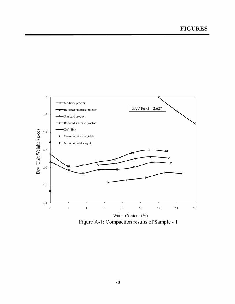
80

FIGURES

Figure A-1: Compaction results of Sample - 1

1.4

1.5

1.6

1.7

1.8

1.9

2

0 2 4 6 8 10 12 14 16

Dry

Uni

t Wei

ght

(g/c

c)

Water Content (%)

Modified proctor

Reduced modified proctor

Standard proctor

Reduced standard proctor

ZAV line

Oven dry vibrating table

Minimum unit weight

ZAV for G = 2.627

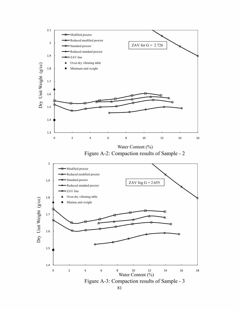
81

Figure A-2: Compaction results of Sample - 2

Figure A-3: Compaction results of Sample - 3

1.3

1.4

1.5

1.6

1.7

1.8

1.9

2

2.1

0 2 4 6 8 10 12 14 16

Dry

Uni

t Wei

ght

(g/c

c)

Water Content (%)

Modified proctor

Reduced modified proctor

Standard proctor

Reduced standard proctor

ZAV line

Oven dry vibrating table

Minimum unit weight

ZAV for G = 2.726

1.4

1.5

1.6

1.7

1.8

1.9

2

0 2 4 6 8 10 12 14 16 18

Dry

Uni

t Wei

ght

(g/c

c)

Water Content (%)

Modified proctor

Reduced modified proctor

Standard proctor

Reduced standard proctor

ZAV line

Oven dry vibrating table

Minimu unit weight

ZAV fog G = 2.655

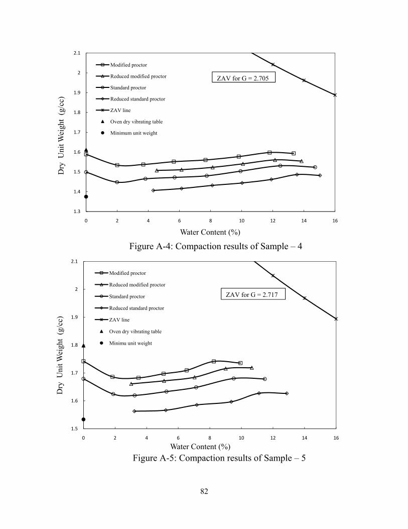
82

Figure A-4: Compaction results of Sample – 4

Figure A-5: Compaction results of Sample – 5

1.3

1.4

1.5

1.6

1.7

1.8

1.9

2

2.1

0 2 4 6 8 10 12 14 16

Dry

Uni

t Wei

ght

(g/c

c)

Water Content (%)

Modified proctor

Reduced modified proctor

Standard proctor

Reduced standard proctor

ZAV line

Oven dry vibrating table

Minimum unit weight

ZAV for G = 2.705

1.5

1.6

1.7

1.8

1.9

2

2.1

0 2 4 6 8 10 12 14 16

Dry

Uni

t Wei

ght

(g/c

c)

Water Content (%)

Modified proctor

Reduced modified proctor

Standard proctor

Reduced standard proctor

ZAV line

Oven dry vibrating table

Minimu unit weight

ZAV for G = 2.717

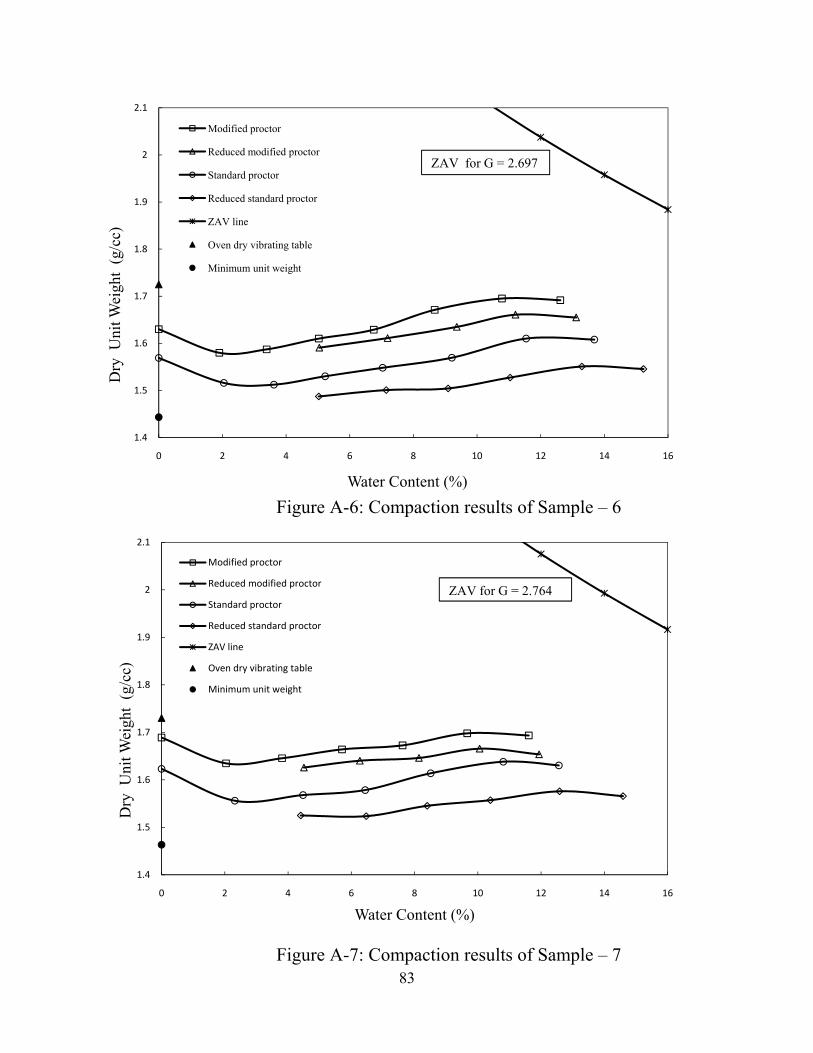
83

Figure A-6: Compaction results of Sample – 6

Figure A-7: Compaction results of Sample – 7

1.4

1.5

1.6

1.7

1.8

1.9

2

2.1

0 2 4 6 8 10 12 14 16

Dry

Uni

t Wei

ght

(g/c

c)

Water Content (%)

Modified proctor

Reduced modified proctor

Standard proctor

Reduced standard proctor

ZAV line

Oven dry vibrating table

Minimum unit weight

ZAV for G = 2.697

1.4

1.5

1.6

1.7

1.8

1.9

2

2.1

0 2 4 6 8 10 12 14 16

Dry

Uni

t Wei

ght

(g/c

c)

Water Content (%)

Modified proctor

Reduced modified proctor

Standard proctor

Reduced standard proctor

ZAV line

Oven dry vibrating table

Minimum unit weight

ZAV for G = 2.764

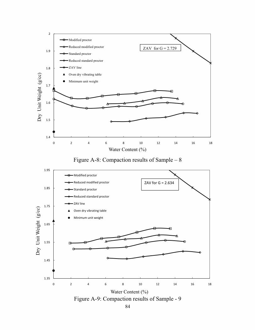
84

Figure A-8: Compaction results of Sample – 8

Figure A-9: Compaction results of Sample - 9

1.4

1.5

1.6

1.7

1.8

1.9

2

0 2 4 6 8 10 12 14 16 18

Dry

Uni

t Wei

ght

(g/c

c)

Water Content (%)

Modified proctor

Reduced modified proctor

Standard proctor

Reduced standard proctor

ZAV line

Oven dry vibrating table

Minimum unit weight

ZAV for G = 2.729

1.35

1.45

1.55

1.65

1.75

1.85

1.95

0 2 4 6 8 10 12 14 16 18

Dry

Uni

t Wei

ght

(g/c

c)

Water Content (%)

Modified proctor

Reduced modified proctor

Standard proctor

Reduced standard proctor

ZAV line

Oven dry vibrating table

Minimum unit weight

ZAV for G = 2.634 

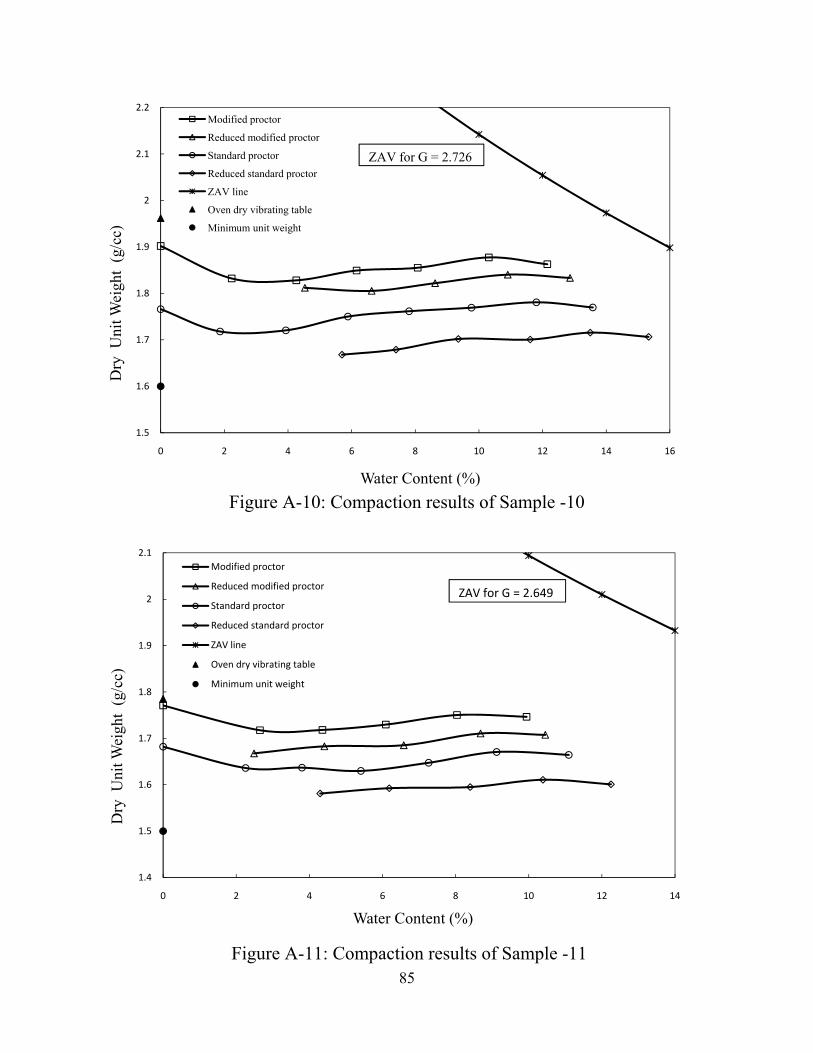
85

Figure A-10: Compaction results of Sample -10

Figure A-11: Compaction results of Sample -11

1.5

1.6

1.7

1.8

1.9

2

2.1

2.2

0 2 4 6 8 10 12 14 16

Dry

Uni

t Wei

ght

(g/c

c)

Water Content (%)

Modified proctor

Reduced modified proctor

Standard proctor

Reduced standard proctor

ZAV line

Oven dry vibrating table

Minimum unit weight

ZAV for G = 2.726

1.4

1.5

1.6

1.7

1.8

1.9

2

2.1

0 2 4 6 8 10 12 14

Dry

Uni

t Wei

ght

(g/c

c)

Water Content (%)

Modified proctor

Reduced modified proctor

Standard proctor

Reduced standard proctor

ZAV line

Oven dry vibrating table

Minimum unit weight

ZAV for G = 2.649 

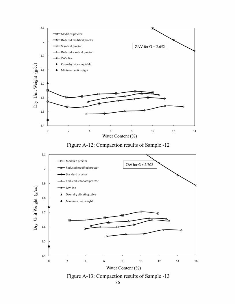
86

Figure A-12: Compaction results of Sample -12

Figure A-13: Compaction results of Sample -13

1.4

1.5

1.6

1.7

1.8

1.9

2

2.1

0 2 4 6 8 10 12 14

Dry

Uni

t Wei

ght

(g/c

c)

Water Content (%)

Modified proctor

Reduced modified proctor

Standard proctor

Reduced standard proctor

ZAV line

Oven dry vibrating table

Minimum unit weight

ZAV for G = 2.652

1.4

1.5

1.6

1.7

1.8

1.9

2

2.1

0 2 4 6 8 10 12 14 16

Dry

Uni

t Wei

ght

(g/c

c)

Water Content (%)

Modified proctor

Reduced modified proctor

Standard proctor

Reduced standard proctor

ZAV line

Oven dry vibrating table

Minimum unit weight

ZAV for G = 2.702

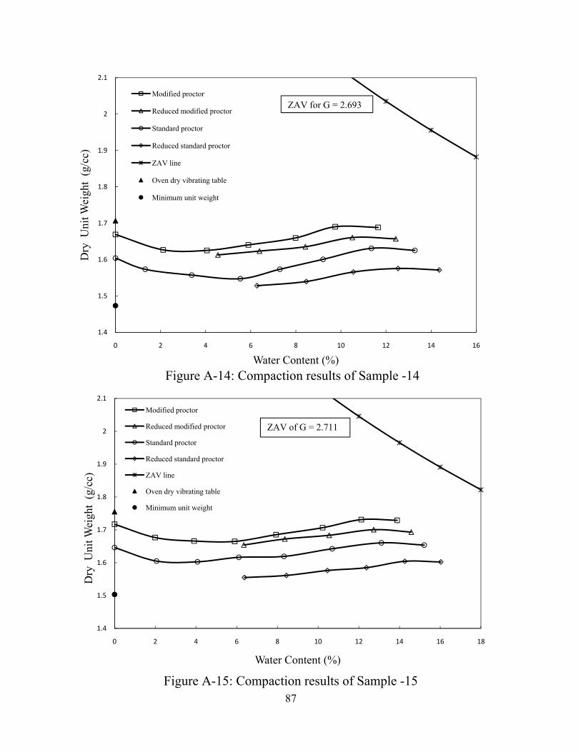
87

Figure A-14: Compaction results of Sample -14

Figure A-15: Compaction results of Sample -15

1.4

1.5

1.6

1.7

1.8

1.9

2

2.1

0 2 4 6 8 10 12 14 16

Dry

Uni

t Wei

ght

(g/c

c)

Water Content (%)

Modified proctor

Reduced modified proctor

Standard proctor

Reduced standard proctor

ZAV line

Oven dry vibrating table

Minimum unit weight

ZAV for G = 2.693

1.4

1.5

1.6

1.7

1.8

1.9

2

2.1

0 2 4 6 8 10 12 14 16 18

Dry

Uni

t Wei

ght

(g/c

c)

Water Content (%)

Modified proctor

Reduced modified proctor

Standard proctor

Reduced standard proctor

ZAV line

Oven dry vibrating table

Minimum unit weight

ZAV of G = 2.711

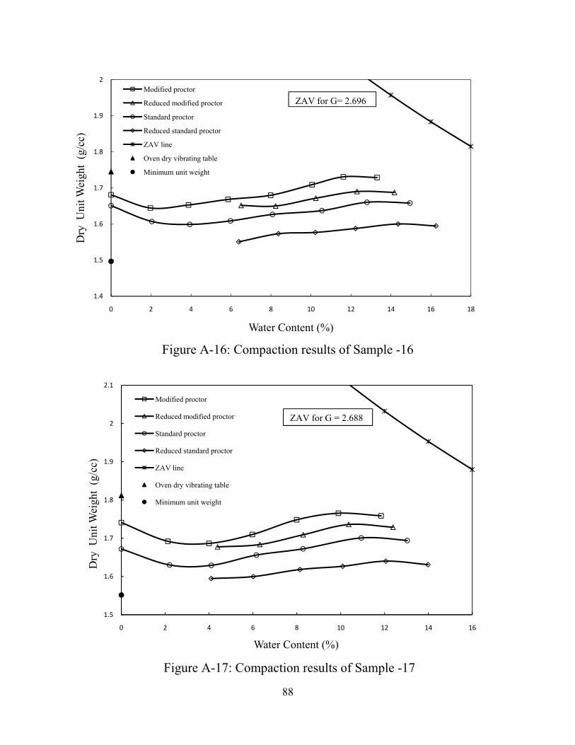
88

Figure A-16: Compaction results of Sample -16

Figure A-17: Compaction results of Sample -17

1.4

1.5

1.6

1.7

1.8

1.9

2

0 2 4 6 8 10 12 14 16 18

Dry

Uni

t Wei

ght

(g/c

c)

Water Content (%)

Modified proctor

Reduced modified proctor

Standard proctor

Reduced standard proctor

ZAV line

Oven dry vibrating table

Minimum unit weight

ZAV for G= 2.696

1.5

1.6

1.7

1.8

1.9

2

2.1

0 2 4 6 8 10 12 14 16

Dry

Uni

t Wei

ght

(g/c

c)

Water Content (%)

Modified proctor

Reduced modified proctor

Standard proctor

Reduced standard proctor

ZAV line

Oven dry vibrating table

Minimum unit weight

ZAV for G = 2.688

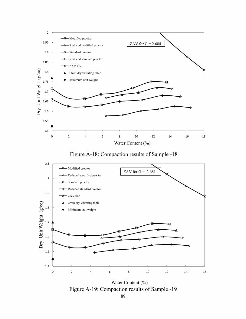
89

Figure A-18: Compaction results of Sample -18

Figure A-19: Compaction results of Sample -19

1.5

1.55

1.6

1.65

1.7

1.75

1.8

1.85

1.9

1.95

2

0 2 4 6 8 10 12 14 16 18

Dry

Uni

t Wei

ght

(g/c

c)

Water Content (%)

Modified proctor

Reduced modified proctor

Standard proctor

Reduced standard proctor

ZAV line

Oven dry vibrating table

Minimum unit weight

ZAV for G = 2.684

1.4

1.5

1.6

1.7

1.8

1.9

2

2.1

0 2 4 6 8 10 12 14 16

Dry

Uni

t Wei

ght

(g/c

c)

Water Content (%)

Modified proctor

Reduced modified proctor

Standard proctor

Reduced standard proctor

ZAV line

Oven dry vibrating table

Minimum unit weight

ZAV for G = 2.681

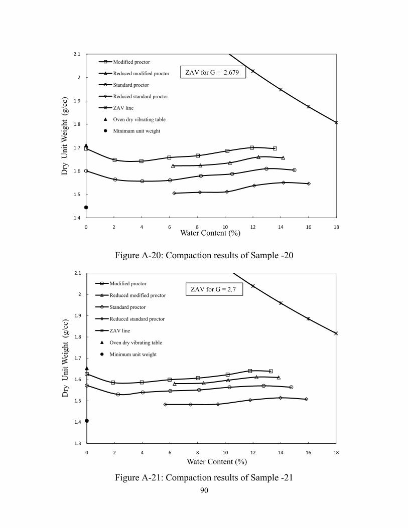
90

Figure A-20: Compaction results of Sample -20

Figure A-21: Compaction results of Sample -21

1.4

1.5

1.6

1.7

1.8

1.9

2

2.1

0 2 4 6 8 10 12 14 16 18

Dry

Uni

t Wei

ght

(g/c

c)

Water Content (%)

Modified proctor

Reduced modified proctor

Standard proctor

Reduced standard proctor

ZAV line

Oven dry vibrating table

Minimum unit weight

ZAV for G = 2.679

1.3

1.4

1.5

1.6

1.7

1.8

1.9

2

2.1

0 2 4 6 8 10 12 14 16 18

Dry

Uni

t Wei

ght

(g/c

c)

Water Content (%)

Modified proctor

Reduced modified proctor

Standard proctor

Reduced standard proctor

ZAV line

Oven dry vibrating table

Minimum unit weight

ZAV for G = 2.7

91

Figure A-22: Compaction results of Sample -22

Figure A-23: Compaction results of Sample -23

1.3

1.4

1.5

1.6

1.7

1.8

1.9

2

2.1

0 2 4 6 8 10 12 14 16 18

Dry

Uni

t Wei

ght

(g/c

c)

Water Content (%)

Modified proctor

Reduced modified proctor

Standard procotor

Reduced standard proctor

ZAV line

Oven dry vibrating table

Minimum unit weight

ZAV for G = 2.707

1.4

1.5

1.6

1.7

1.8

1.9

2

2.1

0 2 4 6 8 10 12 14 16 18

Dry

Uni

t Wei

ght

(g/c

c)

Water Content (%)

Modified proctor

Reduced modified proctor

Standard proctor

Reduced standard proctor

ZAV line

Oven dry vibrating table

Minimum unit weight

ZAV for G = 2.656

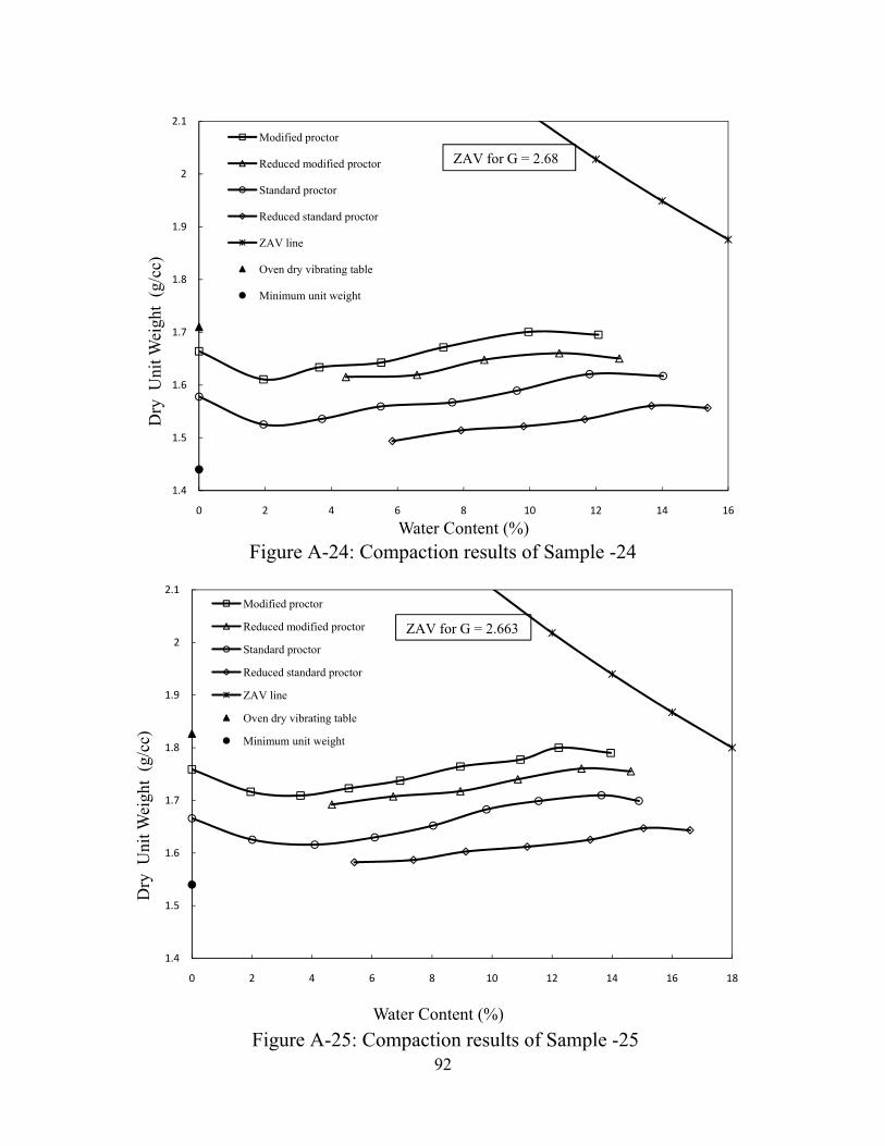
92

Figure A-24: Compaction results of Sample -24

Figure A-25: Compaction results of Sample -25

1.4

1.5

1.6

1.7

1.8

1.9

2

2.1

0 2 4 6 8 10 12 14 16

Dry

Uni

t Wei

ght

(g/c

c)

Water Content (%)

Modified proctor

Reduced modified proctor

Standard proctor

Reduced standard proctor

ZAV line

Oven dry vibrating table

Minimum unit weight

ZAV for G = 2.68

1.4

1.5

1.6

1.7

1.8

1.9

2

2.1

0 2 4 6 8 10 12 14 16 18

Dry

Uni

t Wei

ght

(g/c

c)

Water Content (%)

Modified proctor

Reduced modified proctor

Standard proctor

Reduced standard proctor

ZAV line

Oven dry vibrating table

Minimum unit weight

ZAV for G = 2.663

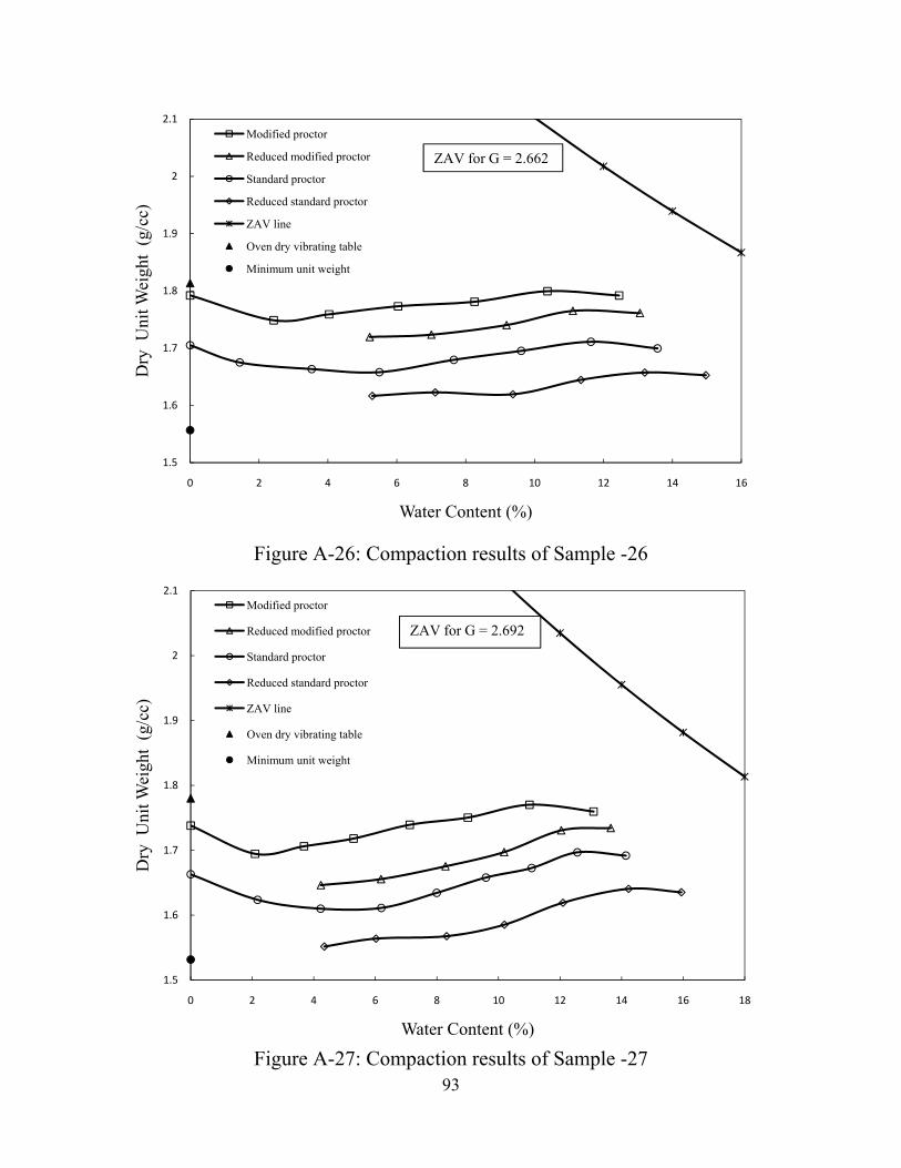
93

Figure A-26: Compaction results of Sample -26

Figure A-27: Compaction results of Sample -27

1.5

1.6

1.7

1.8

1.9

2

2.1

0 2 4 6 8 10 12 14 16

Dry

Uni

t Wei

ght

(g/c

c)

Water Content (%)

Modified proctor

Reduced modified proctor

Standard proctor

Reduced standard proctor

ZAV line

Oven dry vibrating table

Minimum unit weight

ZAV for G = 2.662

1.5

1.6

1.7

1.8

1.9

2

2.1

0 2 4 6 8 10 12 14 16 18

Dry

Uni

t Wei

ght

(g/c

c)

Water Content (%)

Modified proctor

Reduced modified proctor

Standard proctor

Reduced standard proctor

ZAV line

Oven dry vibrating table

Minimum unit weight

ZAV for G = 2.692

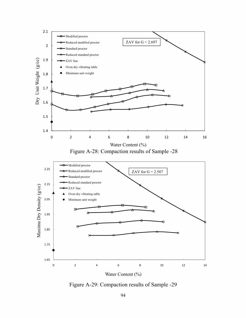
94

Figure A-28: Compaction results of Sample -28

Figure A-29: Compaction results of Sample -29

1.4

1.5

1.6

1.7

1.8

1.9

2

2.1

0 2 4 6 8 10 12 14 16

Dry

Uni

t Wei

ght

(g/c

c)

Water Content (%)

Modified proctor

Reduced modified proctor

Standard proctor

Reduced standard proctor

ZAV line

Oven dry vibrating table

Minimum unit weight

ZAV for G = 2.697

1.65

1.75

1.85

1.95

2.05

2.15

2.25

0 2 4 6 8 10 12 14

Max

imu

Dry

Den

sity

(g/c

c)

Water Content (%)

Modified proctor

Reduced modified proctor

Standard proctor

Reduced standard proctor

ZAV line

Oven dry vibrating table

Minimum unit weight

ZAV for G = 2.587

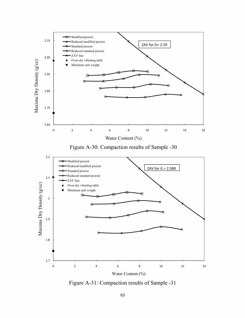
95

Figure A-30: Compaction results of Sample -30

Figure A-31: Compaction results of Sample -31

1.65

1.75

1.85

1.95

2.05

2.15

0 2 4 6 8 10 12 14 16

Max

imu

Dry

Den

sity

(g/c

c)

Water Content (%)

Modified proctorReduced modified proctorStandard proctorReduced standard proctorZAV lineOven dry vibrating tableMinimum unit weight

ZAV for G= 2.59

1.7

1.8

1.9

2

2.1

2.2

0 2 4 6 8 10 12 14

Max

imu

Dry

Den

sity

(g/c

c)

Water Content (%)

Modified proctorReduced modified proctorStandard proctorReduced standard proctorZAV lineOven dry vibrating tableMinimum unit weight

ZAV for G = 2.589

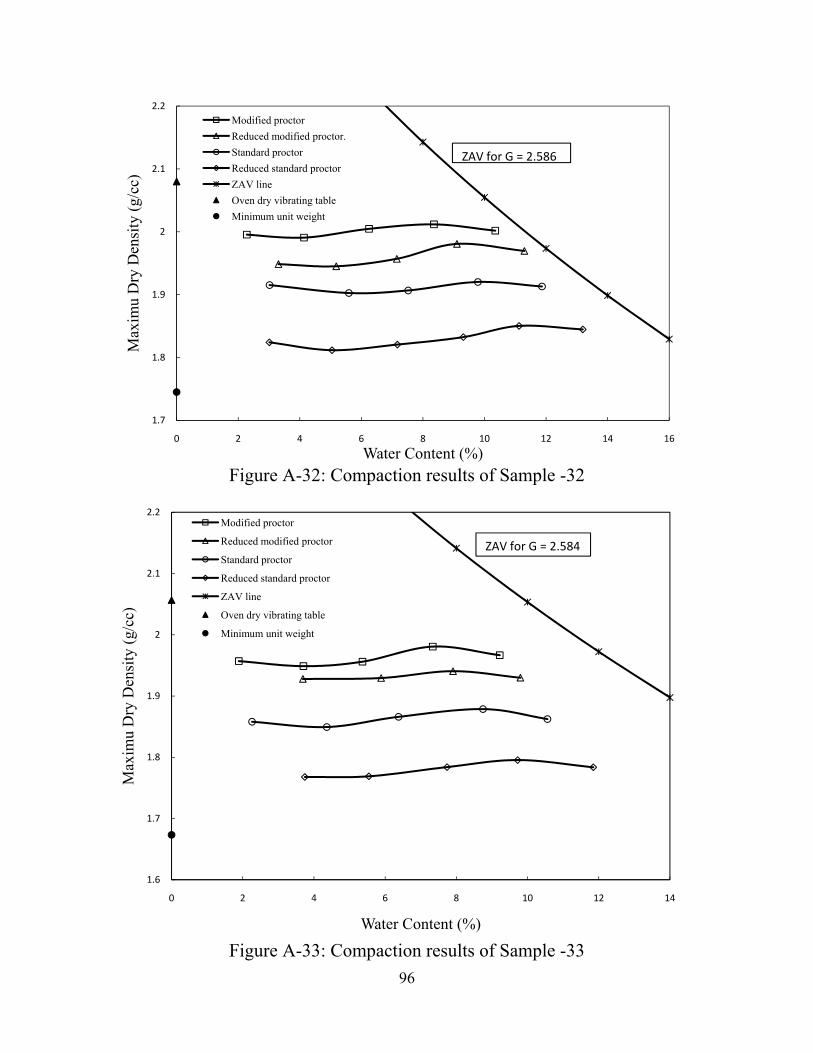
96

Figure A-32: Compaction results of Sample -32

Figure A-33: Compaction results of Sample -33

1.7

1.8

1.9

2

2.1

2.2

0 2 4 6 8 10 12 14 16

Max

imu

Dry

Den

sity

(g/c

c)

Water Content (%)

Modified proctorReduced modified proctor.Standard proctorReduced standard proctorZAV lineOven dry vibrating tableMinimum unit weight

ZAV for G = 2.586

1.6

1.7

1.8

1.9

2

2.1

2.2

0 2 4 6 8 10 12 14

Max

imu

Dry

Den

sity

(g/c

c)

Water Content (%)

Modified proctor

Reduced modified proctor

Standard proctor

Reduced standard proctor

ZAV line

Oven dry vibrating table

Minimum unit weight

ZAV for G = 2.584

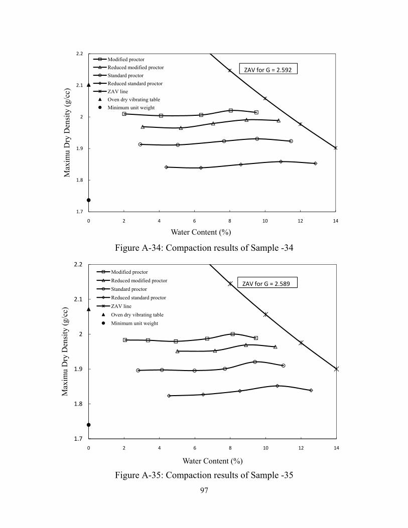
97

Figure A-34: Compaction results of Sample -34

Figure A-35: Compaction results of Sample -35

1.7

1.8

1.9

2

2.1

2.2

0 2 4 6 8 10 12 14

Max

imu

Dry

Den

sity

(g/c

c)

Water Content (%)

Modified proctorReduced modified proctorStandard proctorReduced standard proctorZAV lineOven dry vibrating tableMinimum unit weight

ZAV for G = 2.592

1.7

1.8

1.9

2

2.1

2.2

0 2 4 6 8 10 12 14

Max

imu

Dry

Den

sity

(g/c

c)

Water Content (%)

Modified proctorReduced modified proctorStandard proctorReduced standard proctorZAV lineOven dry vibrating tableMinimum unit weight

ZAV for G = 2.589

98

Figure A-36: Compaction results of Sample -36

Figure A-37: Compaction results of Sample -37

1.7

1.8

1.9

2

2.1

2.2

0 2 4 6 8 10 12 14

Max

imu

Dry

Den

sity

(g/c

c)

Water Content (%)

Modified proctorReduced modified proctorStandard proctorReduced standard proctorZAV lineOven dry vibrating tableMinimum unit weight

ZAV for G = 2.584

1.7

1.8

1.9

2

2.1

2.2

0 2 4 6 8 10 12 14

Max

imu

Dry

Den

sity

(g/c

c)

Water Content (%)

Modified proctorReduced modified proctorStandard proctorReduced standard proctorZAV lineOven dry vibrating tableMinimum unit weight

ZAV for G = 2.578

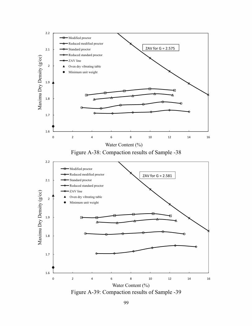
99

Figure A-38: Compaction results of Sample -38

Figure A-39: Compaction results of Sample -39

1.6

1.7

1.8

1.9

2

2.1

2.2

0 2 4 6 8 10 12 14 16

Max

imu

Dry

Den

sity

(g/c

c)

Water Content (%)

Modified proctor

Reduced modified proctor

Standard proctor

Reduced standard proctor

ZAV line

Oven dry vibrating table

Minimum unit weight

ZAV for G = 2.575

1.6

1.7

1.8

1.9

2

2.1

2.2

0 2 4 6 8 10 12 14 16

Max

imu

Dry

Den

sity

(g/c

c)

Water Content (%)

Modified proctor

Reduced modified proctor

Standard proctor

Reduced standard proctor

ZAV line

Oven dry vibrating table

Minimum unit weight

ZAV for G = 2.581

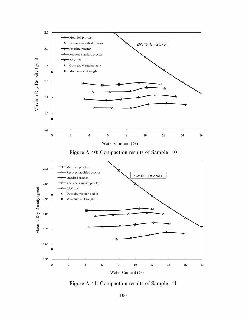
100

Figure A-40: Compaction results of Sample -40

Figure A-41: Compaction results of Sample -41

1.6

1.7

1.8

1.9

2

2.1

2.2

0 2 4 6 8 10 12 14 16

Max

imu

Dry

Den

sity

(g/c

c)

Water Content (%)

Modified proctor

Reduced modified proctor

Standard proctor

Reduced standard proctor

ZAV line

Oven dry vibrating table

Minimum unit weight

ZAV for G = 2.576

1.55

1.65

1.75

1.85

1.95

2.05

2.15

0 2 4 6 8 10 12 14 16 18

Max

imu

Dry

Den

sity

(g/c

c)

Water Content (%)

Modified proctor

Reduced modified proctor

Standard proctor

Reduced standard proctor

ZAV line

Oven dry vibrating table

Minimum unit weight

ZAV for G = 2.581

101

Figure A-42: Compaction results of Sample -42

Figure A-43: Compaction results of Sample -43

1.55

1.65

1.75

1.85

1.95

2.05

2.15

0 2 4 6 8 10 12 14 16 18

Max

imu

Dry

Den

sity

(g/c

c)

Water Content (%)

Modified proctor

Reduced modified proctor

Standard proctor

Reduced standard proctor

ZAV line

Oven dry vibrating table

Minimum unit weight

ZAV for G = 2.556

1.55

1.65

1.75

1.85

1.95

2.05

2.15

0 2 4 6 8 10 12 14 16 18

Max

imu

Dry

Den

sity

(g/c

c)

Water Content (%)

Modified proctor

Reduced modified proctor

Standard proctor

Reduced standard proctor

ZAV line

Oven dry vibrating table

Minimum unit weight

ZAV for G = 2.59

102

Figure A-44: Compaction results of Sample -44

Figure A-45: Compaction results of Sample -45

1.55

1.65

1.75

1.85

1.95

2.05

2.15

0 2 4 6 8 10 12 14 16 18

Max

imu

Dry

Den

sity

(g/c

c)

Water Content (%)

Modified proctor

Reduced modified proctor

Standard proctor

Reduced standard proctor

ZAV line

Oven dry vibrating table

Minimum unit weight

ZAV for G = 2.574

1.6

1.7

1.8

1.9

2

2.1

2.2

0 2 4 6 8 10 12 14 16

Max

imu

Dry

Den

sity

(g/c

c)

Water Content (%)

Modified proctor

Reduced modified proctor

Standard proctor

Reduced standard proctor

ZAV line

Oven dry vibrating table

Minimum unit weight

ZAV for G = 2.607

103

Figure A-46: Compaction results of Sample -46

Figure A-47: Compaction results of Sample -47

1.6

1.7

1.8

1.9

2

2.1

2.2

0 2 4 6 8 10 12 14 16

Max

imu

Dry

Den

sity

(g/c

c)

Water Content (%)

Modified proctor

Reduced modified proctor

Standard proctor

Seduced standard proctor

ZAV line

Oven dry vibrating table

Minimum unit weight

ZAV for G = 2.601

1.7

1.8

1.9

2

2.1

2.2

0 2 4 6 8 10 12 14 16 18

Max

imu

Dry

Den

sity

(g/c

c)

Water Content (%)

Modified proctor

Reduced modified proctor

Standard proctor

Reduced standard proctor

ZAV line

Oven dry vibrating table

Minimum unit weight

ZAV for G = 2.617

104

Figure A-48: Compaction results of Sample -48

Figure A-49: Compaction results of Sample -49

1.65

1.75

1.85

1.95

2.05

2.15

0 2 4 6 8 10 12 14 16 18

Max

imu

Dry

Den

sity

(g/c

c)

Water Content (%)

Modified proctor

Reduced modified proctor

Standard proctor

Reduced standard proctor

ZAV line

Oven dry vibrating table

Minimum unit weight

ZAV for G = 2.557

1.55

1.65

1.75

1.85

1.95

2.05

2.15

0 2 4 6 8 10 12 14 16

Max

imu

Dry

Den

sity

(g/c

c)

Water Content (%)

Modified proctor

Reduced modified proctor

Standard proctor

Reduced standard proctor

ZAV line

Oven dry vibrating table

Minimum unit weight

ZAV for G = 2.566

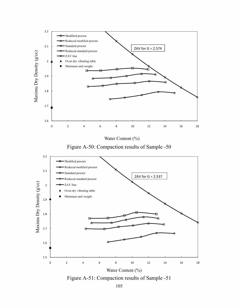
105

Figure A-50: Compaction results of Sample -50

Figure A-51: Compaction results of Sample -51

1.6

1.7

1.8

1.9

2

2.1

2.2

0 2 4 6 8 10 12 14 16 18

Max

imu

Dry

Den

sity

(g/c

c)

Water Content (%)

Modified proctorReduced modified proctorStandard proctorReduced standard proctorZAV lineOven dry vibrating tableMinimum unit weight

ZAV for G = 2.574

1.5

1.6

1.7

1.8

1.9

2

2.1

2.2

0 2 4 6 8 10 12 14 16 18

Max

imu

Dry

Den

sity

(g/c

c)

Water Content (%)

Modified proctor

Reduced modified proctor

Standard proctor

Reduced standard proctor

ZAV line

Oven dry vibrating table

Minimum unit weight

ZAV for G = 2.537

106

Figure A-52: Compaction results of Sample -52

Figure A-53: Compaction results of Sample -53

1.5

1.6

1.7

1.8

1.9

2

2.1

2.2

0 2 4 6 8 10 12 14 16

Max

imu

Dry

Den

sity

(g/c

c)

Water Content (%)

Modified proctor

Reduced modified proctor

Standard proctor

Reduced standard proctor

ZAV line

Oven dry vibrating table

Minimum unit weight

ZAV for G = 2.535

1.5

1.6

1.7

1.8

1.9

2

2.1

2.2

0 2 4 6 8 10 12 14 16

Max

imu

Dry

Den

sity

(g/c

c)

Water Content (%)

Modified proctor

Reduced modified proctor

Standard proctor

Reduced standard proctor

ZAV line

Oven dry vibrating table

Minimum unit weight

ZAV for G = 2.554

107

Figure A-54: Compaction results of Sample -54

Figure A-55: Compaction results of Sample -55

1.5

1.6

1.7

1.8

1.9

2

2.1

2.2

0 2 4 6 8 10 12 14 16

Max

imu

Dry

Den

sity

(g/c

c)

Water Content (%)

Modified proctor

Reduced modified proctor

Standard proctor

Reduced standard proctor

ZAV line

Oven dry vibrating table

Minimum unit weight

ZAV for G = 2.564

1.55

1.65

1.75

1.85

1.95

2.05

2.15

0 2 4 6 8 10 12 14 16

Max

imu

Dry

Den

sity

(g/c

c)

Water Content (%)

Modified proctor

Reduced modified proctor

Standard proctor

Reduced standard proctor

ZAV line

Oven dry vibrating table

Minimum unit weight

ZAV for G = 2.556