ORIGINAL ARTICLE

Prediction of settled water turbidity and optimal coagulant dosagein drinking water treatment plant using a hybrid modelof k-means clustering and adaptive neuro-fuzzy inference system

Chan Moon Kim1• Manukid Parnichkun1

Received: 17 October 2016 /Accepted: 2 February 2017 / Published online: 20 February 2017

� The Author(s) 2017. This article is published with open access at Springerlink.com

Abstract Coagulation is an important process in drinking

water treatment to attain acceptable treated water quality.

However, the determination of coagulant dosage is still a

challenging task for operators, because coagulation is

nonlinear and complicated process. Feedback control to

achieve the desired treated water quality is difficult due to

lengthy process time. In this research, a hybrid of k-means

clustering and adaptive neuro-fuzzy inference system (k-

means-ANFIS) is proposed for the settled water turbidity

prediction and the optimal coagulant dosage determination

using full-scale historical data. To build a well-adaptive

model to different process states from influent water, raw

water quality data are classified into four clusters according

to its properties by a k-means clustering technique. The

sub-models are developed individually on the basis of each

clustered data set. Results reveal that the sub-models

constructed by a hybrid k-means-ANFIS perform better

than not only a single ANFIS model, but also seasonal

models by artificial neural network (ANN). The finally

completed model consisting of sub-models shows more

accurate and consistent prediction ability than a single

model of ANFIS and a single model of ANN based on all

five evaluation indices. Therefore, the hybrid model of k-

means-ANFIS can be employed as a robust tool for

managing both treated water quality and production costs

simultaneously.

Keywords k-means clustering � Adaptive neuro-fuzzy

inference system � Artificial neural network � Coagulantdosage � Water quality � Modeling

Introduction

Drinking water industry has been confronted with two

aspects of strict water quality standards and reduction of

production cost. Coagulation is an important process, and

directly related to production cost and quality in drinking

water treatment plant (WTP). The coagulation is a non-

linear and complicated process, because many physical and

chemical variables influence the process. Conventionally,

the determination of coagulant dosage in drinking WTP is

carried out by experienced operators. However, although

the operators determine coagulant dosage according to

current quality of the raw water and the settled water, the

dosage is still not necessarily optimal, because the opera-

tors cannot handle the errors which will occur after several

hours (Zhang and Stanley 1999). Therefore, it is necessary

to develop decision support models that are able to predict

the treated water quality and the required coagulant dosage.

The models can be considered as process and inverse

process of coagulation. In general, a process model is used

to predict the treated water quality by process inputs, such

as raw water quality and coagulant dosage. This model can

be used to determine coagulant dosage by trial and error

and can be used to understand factors which affect the

process for process analysis and for new operators’ training

(Baxter et al. 2001b). In addition, the process model can be

used to assess in real time the adequacy of coagulant

dosage based on the operator’s experience. Thus, the model

can contribute to ensure the stability of operation. On the

contrary, an inverse process model is used to predict

& Chan Moon Kim

kcm0266@kwater.or.kr

1 School of Engineering and Technology, Asian Institute of

Technology, P.O. Box 4, Klong Luang, Pathumthani 12120,

Thailand

123

Appl Water Sci (2017) 7:3885–3902

DOI 10.1007/s13201-017-0541-5

coagulant dosage using the treated water quality and the

raw water quality. Therefore, the inverse process model

can be used to predict directly the optimal coagulant

dosage based on the raw water quality and the desired

treated water quality.

In recent years, a variety of artificial intelligence (AI)

techniques, such as neural networks and fuzzy inference

systems, have been used in modeling of complex nonlinear

water treatment processes. The use of artificial neural

networks (ANN) has obtained popularity in modeling of

coagulation process in WTP (Gagnon et al. 1997; Roben-

son et al. 2009; Kennedy et al. 2015). ANNs have a great

potential for representing nonlinear complex processes

without structural knowledge of the processes. In the pre-

vious researches, ANNs were applied to develop process

and inverse process models for coagulation to assist oper-

ators to determine coagulant dosage and to optimize the

process. Baxter et al. (1999) developed a full-scale ANN

process model to predict clarifier effluent color at the

Rossdale WTP in Edmonton, Alberta, Canada. Zhang and

Stanley (1999) developed both process and inverse process

ANN models to predict the settled water turbidity and the

optimal alum dosage at the same WTP. Yu et al. (2000)

developed an ANN inverse process model to predict the

coagulant dosage at a WTP in Taipei City, Taiwan. Maier

et al. (2004) developed both process and inverse process

models using multilayer perceptrons (MLP) to predict

several treated water quality parameters and alum dosage at

a WTP in southern Australia. Robenson et al. (2009)

developed an inverse process ANN model to predict the

optimal coagulant dosage with consideration of treated

water quality at Segama WTP in Malaysia. Griffiths and

Andrews (2011a) developed both process and inverse

process seasonal ANN models to predict settled water

turbidity and optimal alum dosage at Elgin Area WTP,

Canada. Kennedy et al. (2015) evaluated four different

hybrid ANN process models for predicting turbidity and

dissolve organic matter removal during coagulation pro-

cess using daily full-scale data at Akron WTP, Ohio, USA.

Another powerful technique for modeling nonlinear

systems is neuro-fuzzy which has an ability to handle

uncertain and noisy data from fuzzy inference system and

learning ability from neural networks. Adaptive neuro-

fuzzy inference system (ANFIS) is one type of neuro-fuzzy

systems (Jang 1993). ANFIS does not have the limitation

of ANN in being trapped in local minima. It can estimate

values that are outside the range of the training data. In

general, the results of ANFIS model are superior than ANN

that they are more accurate and have less uncertainty

(Talebizadeh and Moridnejad 2011). In the literature,

ANFIS has shown effective results in modeling for pre-

dicting coagulant dosage (Gagnon et al. 1997; Wu and Lo

2008; Heddam et al. 2012). However, all these researches

are based on operators’ past behavior corresponding to

influent quality without considering the process output,

such as the settled water turbidity. In other words, none of

previous researches has applied ANFIS models on the

dynamics of coagulation process.

As a result of development of supervisory control and

data acquisition (SCADA), the amount of data collected at

WTP has increased enormously in recent years. In this

situation, clustering technique is a good method for ana-

lyzing huge amount of information by classifying data into

groups. Moreover, it is very useful for categorizing multi-

dimensional data in clusters, allowing users to acquire

effective information in decision making for complex

water treatment processes. Maier et al. (2004) used

Kohonen self-organizing map (SOM) to divide data into

three subsets for developing ANN models. Park et al.

(2008) used k-means clustering to classify data sets in

making decision model for coagulant dosage. Juntunen

et al. (2013) applied SOM and k-means clustering for

modeling water quality in drinking WTP to assess the

essential characteristics of the process. They concluded that

the whole model should be able to adapt to different con-

ditions by making separated sub-models for different states

of the process, because a single uniform model always had

problem in modeling complex relationships in the whole

WTP process. Some studies also demonstrated that models

composed of sub-models could be effective by modeling

each state of the process, such as seasonal models (Gagnon

et al. 1997; Griffiths and Andrews 2011a, b).

The main objective of this research is to develop

enhanced models that are able to predict better the settled

water turbidity and to determine optimal hourly coagulant

dosage on full-scale condition in drinking WTP. To

develop well-adjusted prediction models to different pro-

cess states, k-means clustering method is integrated with

ANFIS technique. Models by ANFIS and ANN are also

developed for performance comparison. The proposed

hybrid of k-means-ANFIS approach is the first attempt in

modeling dynamic coagulation process.

Materials and methods

Treatment process and data set

Bansong WTP is located in Changwon city, South Korea

and operated by Korea water resources corporation (k wa-

ter) which is a government-owned company. Raw water is

supplied through 15.5 km buried pipeline from intake

pump station at Nakdong River. It has treatment capacity

of 120,000 m3 per day and serves population and industrial

complex in Changwon city. Bansong WTP adopts the

conventional treatment process which consists of pre-

3886 Appl Water Sci (2017) 7:3885–3902

123

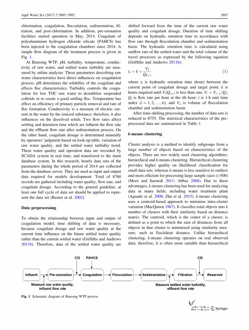
chlorination, coagulation, flocculation, sedimentation, fil-

tration, and post-chlorination. In addition, pre-ozonation

facilities started operation in May, 2014. Coagulant of

polyaluminium hydrogen chloride silicate (PAHCS) has

been injected to the coagulation chambers since 2014. A

simple flow diagram of the treatment process is given in

Fig. 1.

At Bansong WTP, pH, turbidity, temperature, conduc-

tivity of raw water, and settled water turbidity are mea-

sured by online analyzer. These parameters describing raw

water characteristics have direct influences on coagulation

process. pH determines the solubility of the coagulant and

effects floc characteristics. Turbidity controls the coagu-

lation for low TOC raw water to destabilize suspended

colloids or to create a good settling floc. Temperature has

effect on efficiency of primary particle removal and rate of

floc formation. Conductivity is a measure of electric cur-

rent in the water by the ionized substance; therefore, it also

influences on the dissolved solids. Two flow rates affect

settling and detention time which are influent the flow rate

and the effluent flow rate after sedimentation process. On

the other hand, coagulant dosage is determined manually

by operators’ judgment based on look-up table, variation of

raw water quality, and the settled water turbidity trend.

These water quality and operation data are recorded by

SCADA system in real time, and transferred to the main

database system. In this research, hourly data sets of the

parameters during the whole period of 2014 are collected

from the database server. They are used as input and output

data required for models development. Total of 8760

records are gathered including water quality, flow rate, and

coagulant dosage. According to the general guideline, at

least one full cycle of data set should be applied to repre-

sent the data set (Baxter et al. 2002).

Data preprocessing

To obtain the relationship between input and output of

coagulation model, time shifting of data is necessary,

because coagulant dosage and raw water quality at the

current time influence on the future settled water quality

rather than the current settled water (Griffiths and Andrews

2011b). Therefore, data of the settled water quality are

shifted forward from the time of the current raw water

quality and coagulant dosage. Duration of time shifting

depends on hydraulic retention time in accordance with

flow rate through flocculation chamber and sedimentation

basin. The hydraulic retention time is calculated using

outflow rate of the settled water and the total volume of the

travel processes as expressed by the following equation

(Griffiths and Andrews 2011b):

tr ¼ k þ Vk

Qkþ1

ð1Þ

where tr is hydraulic retention time (hour) between the

current point of coagulant dosage and target point; k is

hours required until Vi/Qi?1 is less than one; Vi ¼ Vi�1=Qi;

Qi is flow rate per hour at the ith hour; i is 1-h unit time

index (i ¼ 1; 2; . . .; k); and Vo is volume of flocculation

chamber and sedimentation basin.

After time-shifting processing, the number of data sets is

reduced to 8755. The statistical characteristics of the pre-

processed data are summarized in Table 1.

k-means clustering

Cluster analysis is a method to identify subgroups from a

large number of objects based on characteristics of the

objects. There are two widely used clustering algorithms:

hierarchical and k-means clustering. Hierarchical clustering

provides higher quality on likelihood classification for

small data sets, whereas k-means is less sensitive to outliers

and more efficient for processing large sample sizes ([500)

(Mooi and Sarstedt 2011; Abbas 2008). Due to these

advantages, k-means clustering has been used for analyzing

data in many fields, including water treatment plant

(Aguado et al. 2008; Zhu et al. 2015). k-means clustering

uses a centroid-based approach to minimize intra-cluster

variation (MacQueen 1967). It classifies total objects into k

number of clusters with their similarity based on distance

matrix. The centroid, which is the center of a cluster, is

defined as a point to which the sum of distances from all

objects in that cluster is minimized using similarity mea-

sure, such as Euclidean distance. Unlike hierarchical

clustering, k-means clustering operates on real observed

data; therefore, it is often more suitable than hierarchical

Fig. 1 Schematic diagram of Bansong WTP process

Appl Water Sci (2017) 7:3885–3902 3887

123

clustering for large amounts of data. k-means clustering

algorithm proceeds as follows (MacQueen 1967):

J ¼Xk

i¼1

X

xj 2 Si

xj � c2i�� �� ð2Þ

where J is the objective function; xj is data vector given a

set of observations (j ¼ 1; 2; . . .; nÞ; k is the number of

clusters; Si is cluster; and ci is cluster center.

1. Define k clusters with certain rules, and assign

k random data vectors as the initial centroid of clusters.

2. Assign each object to the nearest cluster by calculating

the distance between each object and the correspond-

ing centroid vector.

3. Update a new centroid vector for each cluster.

4. If the result meets termination criterion (value of

minimal objective function or maximum iteration

number), the algorithm stops, otherwise, go to step 2.

Adaptive neuro fuzzy inference system (ANFIS)

Neuro-fuzzy network is composed of artificial neural net-

work and fuzzy inference system. The Takagi–Sugeno is a

famous fuzzy inference model for data-based fuzzy mod-

eling (Michael 2005). The Sugeno fuzzy model generates

fuzzy rules from a given input and output data set (Takagi

and Sugeno 1985). ANFIS introduced by Jang (1993) is

capable of approximating any continuous functions on a

compact set to any degrees of accuracy, thus it has shown

good prediction performance in various areas related to

water research in the literature (Shu and Ouarda 2008; Al-

Abadi 2014). ANFIS combines the fuzzy inference system

with multilayer feed-forward neural network as a general

structure, where if–then rules with proper membership

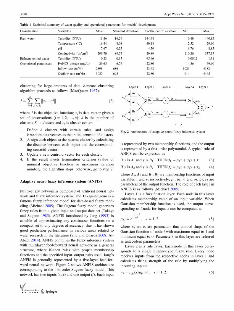
functions and the specified input–output pairs used. Jang’s

ANFIS is generally represented by a five-layer feed-for-

ward neural network. Figure 2 shows ANFIS architecture

corresponding to the first-order Sugeno fuzzy model. This

network has two inputs (x, y) and one output (f). Each input

is represented by two membership functions, and the output

is represented by a first-order polynomial. A typical rule of

ANFIS can be expressed as

If x is A1 and y is B1 THEN f1 ¼ p1xþ q1yþ r1 ð3ÞIf x is A2 and y is B2 THEN f2 ¼ p2xþ q2yþ r2 ð4Þ

where A1, A2 and B1, B2 are membership functions of input

variables x and y, respectively; p1, q1, r1 and p2, q2, r2 are

parameters of the output function. The role of each layer in

ANFIS is as follows (Michael 2005):

Layer 1 is a fuzzification layer. Each node in this layer

calculates membership value of an input variable. When

Gaussian membership function is used, the output corre-

sponding to i node for input x can be computed as

lAi¼ e

�ðx�ciÞ2

2r2i ; i ¼ 1; 2 ð5Þ

where ri are ci are parameters that control shape of the

Gaussian function of node i with maximum equal to 1 and

minimum equal to 0. Parameters in this layer are referred

as antecedent parameters.

Layer 2 is a rule layer. Each node in this layer corre-

sponds to a single Sugeno-type fuzzy rule. Every node

receives inputs from the respective nodes in layer 1 and

calculates firing strength of the rule by multiplying the

incoming inputs:

wi ¼ lAiðxÞlBi

ðyÞ; i ¼ 1; 2: ð6Þ

Table 1 Statistical summary of water quality and operational parameters for models’ development

Classification Variables Mean Standard deviation Coefficient of variation Min Max

Raw water Turbidity (NTU) 11.46 16.56 144.48 0.49 440.85

Temperature (�C) 16.44 8.08 49.18 2.52 29.90

pH 7.67 0.35 4.59 6.76 8.85

Conductivity (ls/cm2) 299.70 89.57 29.89 110.20 537.17

Effluent settled water Turbidity (NTU) 0.23 0.15 65.66 0.0002 1.31

Operational parameters PAHCS dosage (mg/L) 29.65 6.76 22.80 14.36 69.60

Inflow rate (m3/h) 2898 686 23.68 1029 4188

Outflow rate (m3/h) 3037 693 22.80 914 4445

Fig. 2 Architecture of adaptive neuro fuzzy inference system

3888 Appl Water Sci (2017) 7:3885–3902

123

Layer 3 is a normalization layer. Each node in this layer

calculates normalized firing strength from the ratio of each

node’s firing strength to the sum of all rules’ firing

strengths. It represents the degree of contribution of a given

rule to the final result. The ith node of this layer is

computed as

wi ¼wi

w1 þ w2

; i ¼ 1; 2: ð7Þ

Layer 4 is a defuzzification layer. Each node in this layer

is connected to the respective node in layer 3, and also the

initial inputs x and y. Thus, the output of each node in this

layer is determined as the product of the normalized firing

strength and the first-order polynomial function:

wifi ¼ wiðpixþ qiyþ riÞ; i ¼ 1; 2 ð8Þ

where pi, qi, and ri are consequent parameters of rule i.

Layer 5 is a summation layer. This neuron computes the

sum of outputs of all defuzzification nodes and produces

the overall output, f:

f ¼X

i

wifi ¼P

i wifiPi wi

: ð9Þ

The parameters for optimization in ANFIS are the

antecedent parameters {ri; ci} which represent the shape

and location of the input membership functions, and the

consequent parameters {pi, qi, ri} which describe the

overall output of the system. In ANFIS, the parameters

associated the membership functions of input and output

are trained using a hybrid learning algorithm that combines

the least-square estimator and the gradient descent method

(Jang 1993). Identification of parameters associated with

the consequent part of fuzzy rules in the complicated

system is important. There are two most commonly used

models for identification of fuzzy inference system in

ANFIS. They are grid partition and clustering methods.

The grid partition method has a critical drawback that all

combinations of membership functions for each input make

excessive number of rules; therefore, it causes a huge

amount of calculation and inferior performance to

clustering method in predicting coagulant dosage

(Heddam et al. 2012). Thus, these parameters are usually

extracted from the observed data using clustering method.

Among various clustering methods, subtractive clustering

method is the best for the condition, where the number of

clusters for a given data set is not known (Talebizadeh and

Moridnejad 2011).

Artificial neural network (ANN)

Artificial neural network is a massive parallel information

processing system composed of a number of simple pro-

cessing elements known as neurons or nodes (Haykin

1998). MLP is the most popularly used feed-forward

hierarchical ANN which is used to map any random input

with the corresponding output. Therefore, MLP has been

used for a variety of studies for modeling and prediction on

water research (Mondal et al. 2012; Al-Abadi 2014). MLP

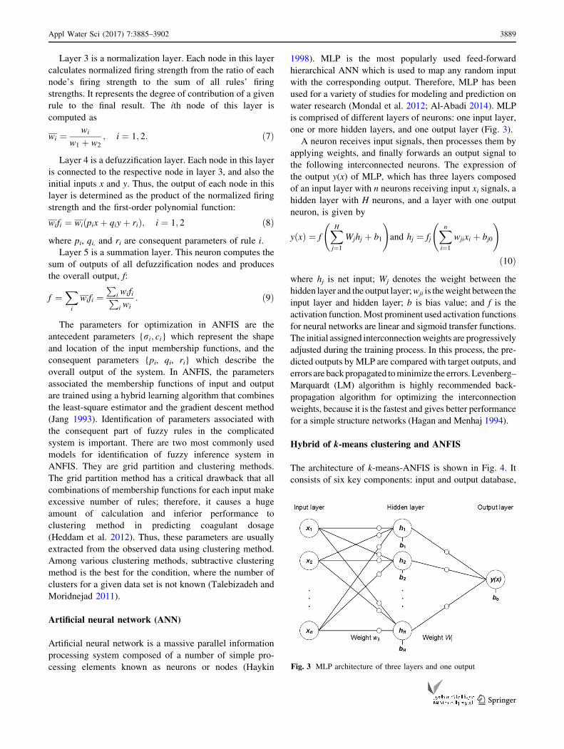
is comprised of different layers of neurons: one input layer,

one or more hidden layers, and one output layer (Fig. 3).

A neuron receives input signals, then processes them by

applying weights, and finally forwards an output signal to

the following interconnected neurons. The expression of

the output y(x) of MLP, which has three layers composed

of an input layer with n neurons receiving input xi signals, a

hidden layer with H neurons, and a layer with one output

neuron, is given by

yðxÞ ¼ fXH

j¼1

Wjhj þ b1

!and hj ¼ fj

Xn

i¼1

wjixi þ bj0

!

ð10Þ

where hj is net input; Wj denotes the weight between the

hidden layer and the output layer;wji is theweight between the

input layer and hidden layer; b is bias value; and f is the

activation function.Most prominent used activation functions

for neural networks are linear and sigmoid transfer functions.

The initial assigned interconnectionweights are progressively

adjusted during the training process. In this process, the pre-

dicted outputs by MLP are compared with target outputs, and

errors are backpropagated tominimize the errors. Levenberg–

Marquardt (LM) algorithm is highly recommended back-

propagation algorithm for optimizing the interconnection

weights, because it is the fastest and gives better performance

for a simple structure networks (Hagan and Menhaj 1994).

Hybrid of k-means clustering and ANFIS

The architecture of k-means-ANFIS is shown in Fig. 4. It

consists of six key components: input and output database,

Fig. 3 MLP architecture of three layers and one output

Appl Water Sci (2017) 7:3885–3902 3889

123

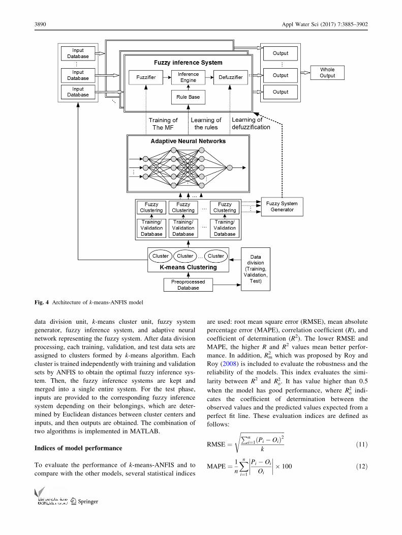
data division unit, k-means cluster unit, fuzzy system

generator, fuzzy inference system, and adaptive neural

network representing the fuzzy system. After data division

processing, each training, validation, and test data sets are

assigned to clusters formed by k-means algorithm. Each

cluster is trained independently with training and validation

sets by ANFIS to obtain the optimal fuzzy inference sys-

tem. Then, the fuzzy inference systems are kept and

merged into a single entire system. For the test phase,

inputs are provided to the corresponding fuzzy inference

system depending on their belongings, which are deter-

mined by Euclidean distances between cluster centers and

inputs, and then outputs are obtained. The combination of

two algorithms is implemented in MATLAB.

Indices of model performance

To evaluate the performance of k-means-ANFIS and to

compare with the other models, several statistical indices

are used: root mean square error (RMSE), mean absolute

percentage error (MAPE), correlation coefficient (R), and

coefficient of determination (R2). The lower RMSE and

MAPE, the higher R and R2 values mean better perfor-

mance. In addition, Rm2 which was proposed by Roy and

Roy (2008) is included to evaluate the robustness and the

reliability of the models. This index evaluates the simi-

larity between R2 and R2o. It has value higher than 0.5

when the model has good performance, where R2o indi-

cates the coefficient of determination between the

observed values and the predicted values expected from a

perfect fit line. These evaluation indices are defined as

follows:

RMSE ¼

ffiffiffiffiffiffiffiffiffiffiffiffiffiffiffiffiffiffiffiffiffiffiffiffiffiffiffiffiffiffiffiPni¼1ðPi � OiÞ2

k

s

ð11Þ

MAPE ¼ 1

n

Xn

i¼1

Pi � Oi

Oi

����

����� 100 ð12Þ

Fig. 4 Architecture of k-means-ANFIS model

3890 Appl Water Sci (2017) 7:3885–3902

123

R ¼Pn

i¼1ðOi � OÞðPi � PÞffiffiffiffiffiffiffiffiffiffiffiffiffiffiffiffiffiffiffiffiffiffiffiffiffiffiffiffiffiffiffiffiffiffiffiffiffiffiffiffiffiffiffiffiffiffiffiffiffiffiffiffiffiffiffiffiffiffiffiffiPni¼1ðOi � OÞ2

Pni¼1ðPi � PÞ2

q ð13Þ

R2 ¼ 1�Pn

i¼1ðOi � PiÞ2Pni¼1ðOi � OÞ2

ð14Þ

R2m ¼ R2 1�

ffiffiffiffiffiffiffiffiffiffiffiffiffiffiffiffiffiffiffiR2 � R2

o

�� ��q� �

ð15Þ

where n is the number of data; Pi is the predicted value

and Oi is the observed value; and P and O are the average

values of the predicted and observed values,

respectively.

Result and discussion

Variations of water quality and coagulant dosage

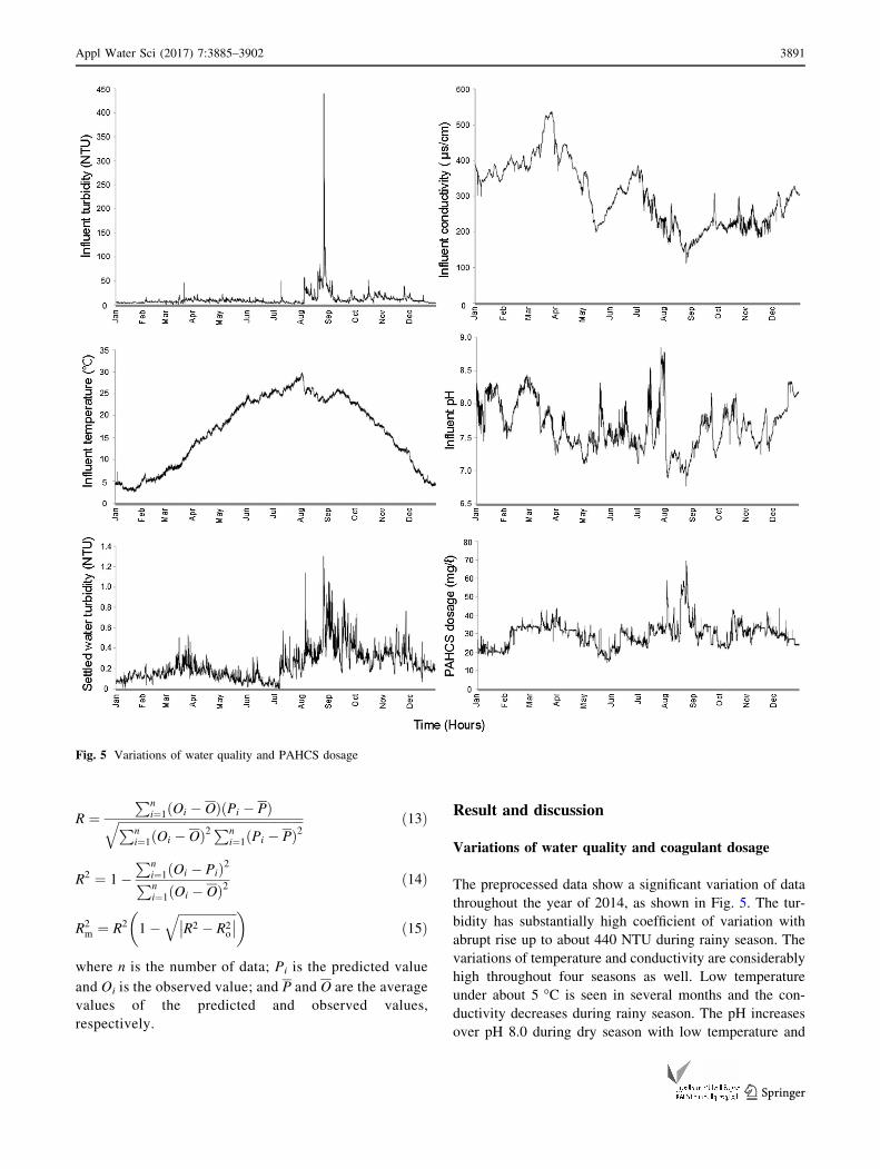
The preprocessed data show a significant variation of data

throughout the year of 2014, as shown in Fig. 5. The tur-

bidity has substantially high coefficient of variation with

abrupt rise up to about 440 NTU during rainy season. The

variations of temperature and conductivity are considerably

high throughout four seasons as well. Low temperature

under about 5 �C is seen in several months and the con-

ductivity decreases during rainy season. The pH increases

over pH 8.0 during dry season with low temperature and

Fig. 5 Variations of water quality and PAHCS dosage

Appl Water Sci (2017) 7:3885–3902 3891

123

some periods in summer. The variation of the settled water

turbidity is high due to the large variation of the raw water

turbidity. It exceeds over 1 NTU in some cases during

summer season. The PAHCS is dosed at the rate from

around 14–40 mg/L during non-rainy seasons; however,

around 70 mg/L is dosed during rainy season.

The results of k-means clustering on raw water

quality

To identify distinctive process states according to the

influent water, four-dimensional raw water quality is

classified by k-means clustering. In general, data normal-

ization is useful to generate good clusters and to improve

the accuracy of clustering. The raw water quality data are

converted into specific ranges by Z-score method, so that

different ranges of four parameters can be treated equally

for fair comparison. Z-score conversion is effective for k-

means algorithm (Mohamad and Usman 2013). The origi-

nal data (x) are normalized using the average value (x) and

standard deviation (s) as shown in Eq. (15). As the result,

all parameters have zero mean and unit variance:

Z - score ¼ x� x

s: ð16Þ

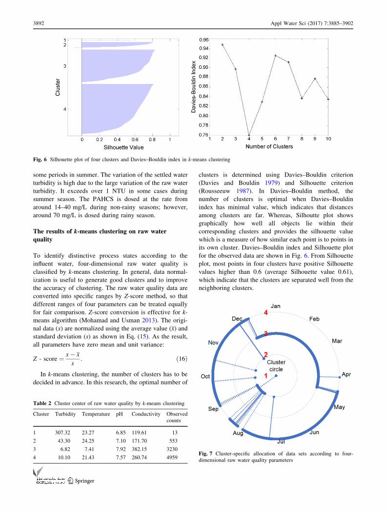
In k-means clustering, the number of clusters has to be

decided in advance. In this research, the optimal number of

clusters is determined using Davies–Bouldin criterion

(Davies and Bouldin 1979) and Silhouette criterion

(Rousseeuw 1987). In Davies–Bouldin method, the

number of clusters is optimal when Davies–Bouldin

index has minimal value, which indicates that distances

among clusters are far. Whereas, Silhoutte plot shows

graphically how well all objects lie within their

corresponding clusters and provides the silhouette value

which is a measure of how similar each point is to points in

its own cluster. Davies–Bouldin index and Silhouette plot

for the observed data are shown in Fig. 6. From Silhouette

plot, most points in four clusters have positive Silhouette

values higher than 0.6 (average Silhouette value 0.61),

which indicate that the clusters are separated well from the

neighboring clusters.

Fig. 6 Silhouette plot of four clusters and Davies–Bouldin index in k-means clustering

Table 2 Cluster center of raw water quality by k-means clustering

Cluster Turbidity Temperature pH Conductivity Observed

counts

1 307.32 23.27 6.85 119.61 13

2 43.30 24.25 7.10 171.70 553

3 6.82 7.41 7.92 382.15 3230

4 10.10 21.43 7.57 260.74 4959Fig. 7 Cluster-specific allocation of data sets according to four-

dimensional raw water quality parameters

3892 Appl Water Sci (2017) 7:3885–3902

123

These clusters represent four different states of raw

water quality and can be characterized manifestly as center

vectors of the clusters, as shown in Table 2. Cluster 1

which is the smallest cluster represents extremely high

turbidity, the lowest pH, and conductivity during rainy

summer season. Cluster 2 describes raw water quality with

high turbidity, low-to-medium pH, and the highest tem-

perature from summer to late fall season. Cluster 3 refers to

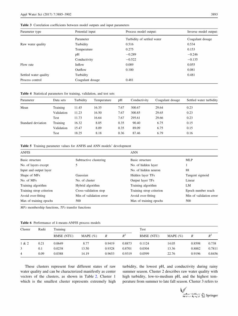
Table 3 Correlation coefficients between model outputs and input parameters

Parameter type Potential input Process model output: Inverse model output:

Parameter Turbidity of settled water Coagulant dosage

Raw water quality Turbidity 0.516 0.534

Temperature 0.275 0.153

pH -0.289 -0.246

Conductivity -0.522 -0.135

Flow rate Inflow 0.089 0.055

Outflow 0.100 0.081

Settled water quality Turbidity 0.481

Process control Coagulant dosage 0.481

Table 4 Statistical parameters for training, validation, and test sets

Parameter Data sets Turbidity Temperature pH Conductivity Coagulant dosage Settled water turbidity

Mean Training 11.45 16.35 7.67 300.67 29.64 0.23

Validation 11.23 16.50 7.67 300.85 29.65 0.23

Test 11.73 16.64 7.67 295.61 29.66 0.23

Standard deviation Training 16.32 8.05 0.35 90.40 6.75 0.15

Validation 15.47 8.09 0.35 89.09 6.75 0.15

Test 18.25 8.18 0.36 87.46 6.79 0.16

Table 5 Training parameter values for ANFIS and ANN models’ development

ANFIS ANN

Basic structure Subtractive clustering Basic structure MLP

No. of layers except 5 No. of hidden layer 1

Input and output layer No. of hidden neuron 88

Shape of MFs Gaussian Hidden layer TFs Tangent sigmoid

No. of MFs No. of cluster Output layer TFs Linear

Training algorithm Hybrid algorithm Training algorithm LM

Training strop criterion Cross-validation stop Training strop criterion Epoch number reach

Avoid over-fitting Min of validation error Avoid over-fitting Min of validation error

Max of training epochs 500 Max of training epochs 500

MFs membership functions, TFs transfer functions

Table 6 Performance of k-means-ANFIS process models

Cluster Radii Training Test

RMSE (NTU) MAPE (%) R R2 RMSE (NTU) MAPE (%) R R2

1 & 2 0.21 0.0649 8.77 0.9419 0.8873 0.1124 14.05 0.8598 0.738

3 0.1 0.0238 13.50 0.9328 0.8701 0.0304 13.36 0.8882 0.7811

4 0.09 0.0388 14.19 0.9653 0.9319 0.0599 22.76 0.9196 0.8456

Appl Water Sci (2017) 7:3885–3902 3893

123

the water state in which temperature is the lowest, pH is the

highest, and turbidity is the lowest during cold season that

spans from December to April. Cluster 4 includes the lar-

gest sample size and the most frequent condition. In cluster

4, the data of water quality spread from April to December,

representing water quality that is the closest to the average

but medium-to-high temperature value. The whole data sets

of a year are categorized successfully according to the

distinct characteristics of the parameters by k-means

algorithm, as shown in Fig. 7. From the viewpoint of

models development, the number of data in cluster 1 is not

sufficient for good training in neural networks compared

with the other clusters; therefore, the data are integrated

with cluster 2.

ANFIS and ANN models

To determine contribution of the input parameters to the

models, the correlation coefficients (R) are calculated, as

shown in Table 3. High turbidity impact is shown with

high value of R. Conductivity has the most influence on

turbidity of the settled water, while it has the least influence

on coagulant dosage. Both in and out flow rates are low

influential parameters. Consequently, four raw water

quality parameters and coagulant dosage are selected as

input of the process model, and four raw water quality

parameters and settled water turbidity are chosen as input

of the inverse process model. The value of R which is

higher than 0.1 is set as the threshold for selecting input

parameters in the models (Chen and Liu 2014).

In good data division, statistical properties, such as

mean and standard deviation of subsets of the data, should

be similar to guarantee that the subsets represent the whole

population of study domain (Sahoo et al. 2012). In this

research, 8755 data are divided into three subsets using the

method proposed by Baxter et al. (2001a) by dividing data

at the ratio of 3:1:1 for training, validation, and test sets,

respectively. As the result, 8755 data are divided into 5253,

1751, and 1751 data sets for the training, validation, and

test, respectively (Table 4).

ANFIS model is developed using genfis2 command in

Fuzzy Logic Toolbox of MATLAB, which generates fuzzy

inference system structure from data using subtractive

clustering algorithm. First-order Sugeno model is applied

as fuzzy inference system structure. In subtractive clus-

tering, the range of a cluster in each dimension is

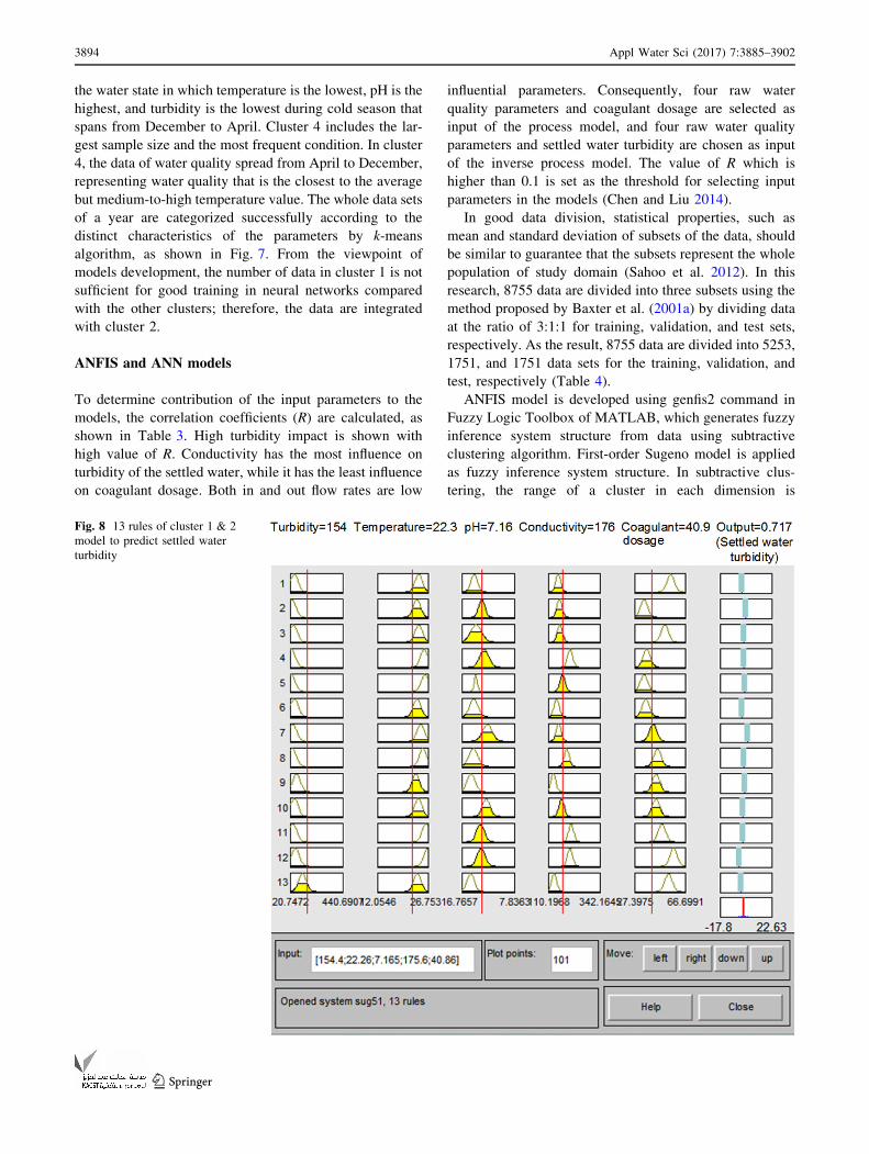
Fig. 8 13 rules of cluster 1 & 2

model to predict settled water

turbidity

3894 Appl Water Sci (2017) 7:3885–3902

123

controlled by radius parameter, and thus, finding optimal

radius is important for subtractive clustering algorithm

(Chiu 1994). In this research, the values from 0.07 to 0.5

(with an increment of 0.01) are investigated to find the

optimal radius value which has the best performance

evaluation index on the test phase. ANN model is also

developed by Neural Network Toolbox in MATLAB. The

number of hidden neurons is determined using the rule that

the ratio of the number of training data to the number of

connection weights should be 10 to 1 (Weigend et al.

1990). The parameters for ANFIS and ANN used in model

development are summarized in Table 5.

Simulation results of k-means-ANFIS models

The performances of three process models by k-means-

ANFIS are presented in Table 6. According to the optimal

cluster radii, each inference system applies 13, 55, and 113

linguistic rules, respectively. Figure 8 shows 13 rules of

cluster 1 & 2 model from fuzzy logic toolbox interface in

MATLAB. With this interface tool, the settled water tur-

bidity can be estimated from the five given input values.

According to the evaluation results, all sub-models have

correlation coefficients higher than 0.8, which represent

strong correlation between the observed and predicted

values. Cluster 1 & 2 model shows the lowest performance,

and it is caused by the biggest variations of turbidity in raw

and settled water (0.16–1.30 NTU) with the smallest

number of data. The model of cluster 3 has the best per-

formance considered from RMSE and MAPE, while the

model of cluster 4 has the best performance considered

from R and R2. Particularly, the R2 value of cluster 4 model

is over 0.8, which indicates that the model is very good

(Shu and Quarda 2008).

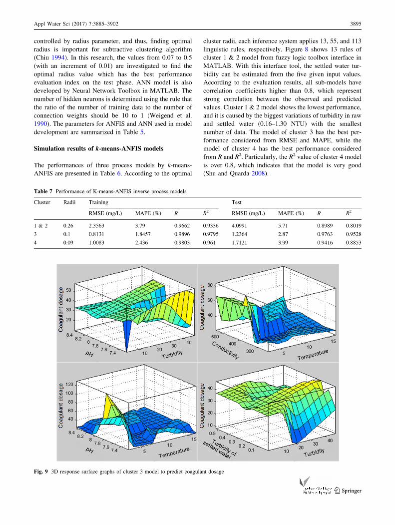
Table 7 Performance of K-means-ANFIS inverse process models

Cluster Radii Training Test

RMSE (mg/L) MAPE (%) R R2 RMSE (mg/L) MAPE (%) R R2

1 & 2 0.26 2.3563 3.79 0.9662 0.9336 4.0991 5.71 0.8989 0.8019

3 0.1 0.8131 1.8457 0.9896 0.9795 1.2364 2.87 0.9763 0.9528

4 0.09 1.0083 2.436 0.9803 0.961 1.7121 3.99 0.9416 0.8853

Fig. 9 3D response surface graphs of cluster 3 model to predict coagulant dosage

Appl Water Sci (2017) 7:3885–3902 3895

123

The evaluation results of three inverse process models

by k-means-ANFIS are shown in Table 7. According to

the optimal cluster radii, the inference systems apply 8,

55, and 113 linguistic rules in the models, respectively.

All models show accurate prediction ability with R and R2

values higher than 0.8. The clusters 1 & 2 model also

shows the lowest performance among the three models.

This is caused by the same reason as the process model:

wide coagulant dosage range (27.39–69.59 mg/L), with

the smallest number of data. The model of cluster 3 has

the best performance in all evaluation indices. Figure 9

illustrates 3D response surface graphs of cluster 3 model.

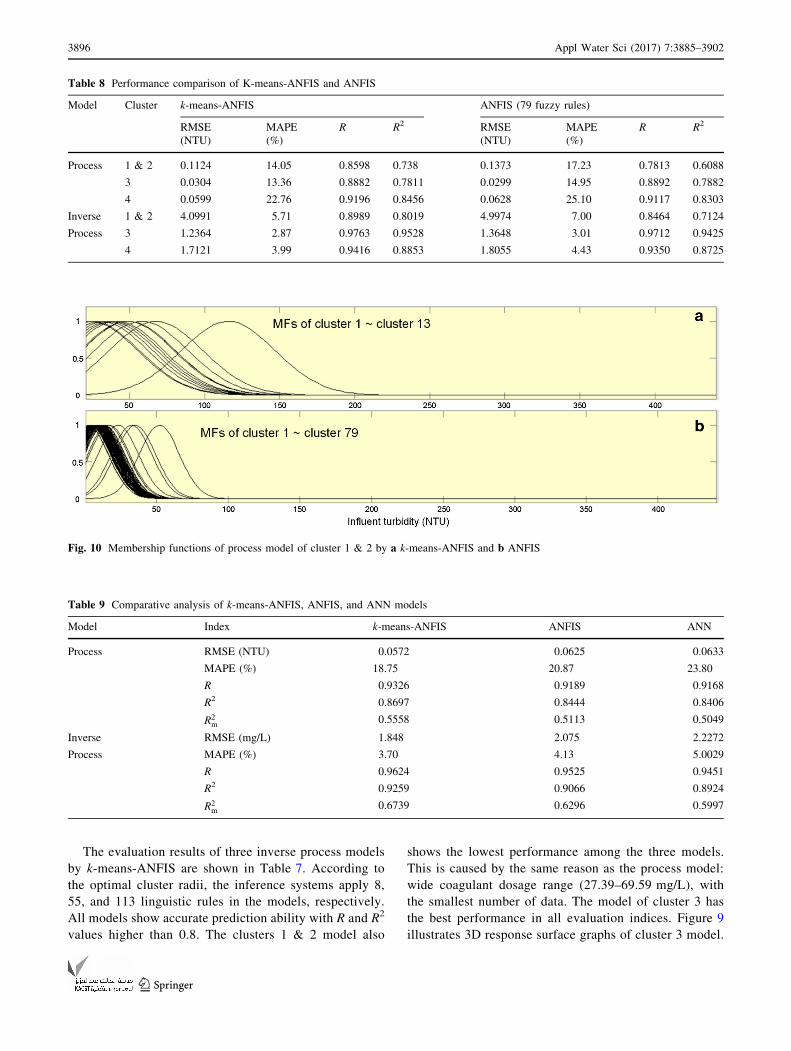
Table 8 Performance comparison of K-means-ANFIS and ANFIS

Model Cluster k-means-ANFIS ANFIS (79 fuzzy rules)

RMSE

(NTU)

MAPE

(%)

R R2 RMSE

(NTU)

MAPE

(%)

R R2

Process 1 & 2 0.1124 14.05 0.8598 0.738 0.1373 17.23 0.7813 0.6088

3 0.0304 13.36 0.8882 0.7811 0.0299 14.95 0.8892 0.7882

4 0.0599 22.76 0.9196 0.8456 0.0628 25.10 0.9117 0.8303

Inverse 1 & 2 4.0991 5.71 0.8989 0.8019 4.9974 7.00 0.8464 0.7124

Process 3 1.2364 2.87 0.9763 0.9528 1.3648 3.01 0.9712 0.9425

4 1.7121 3.99 0.9416 0.8853 1.8055 4.43 0.9350 0.8725

Fig. 10 Membership functions of process model of cluster 1 & 2 by a k-means-ANFIS and b ANFIS

Table 9 Comparative analysis of k-means-ANFIS, ANFIS, and ANN models

Model Index k-means-ANFIS ANFIS ANN

Process RMSE (NTU) 0.0572 0.0625 0.0633

MAPE (%) 18.75 20.87 23.80

R 0.9326 0.9189 0.9168

R2 0.8697 0.8444 0.8406

R2m

0.5558 0.5113 0.5049

Inverse RMSE (mg/L) 1.848 2.075 2.2272

Process MAPE (%) 3.70 4.13 5.0029

R 0.9624 0.9525 0.9451

R2 0.9259 0.9066 0.8924

R2m

0.6739 0.6296 0.5997

3896 Appl Water Sci (2017) 7:3885–3902

123

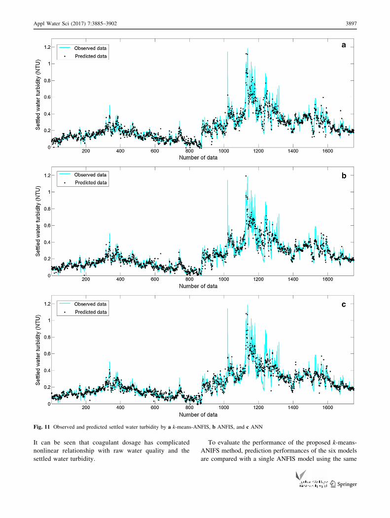
It can be seen that coagulant dosage has complicated

nonlinear relationship with raw water quality and the

settled water turbidity.

To evaluate the performance of the proposed k-means-

ANIFS method, prediction performances of the six models

are compared with a single ANFIS model using the same

Fig. 11 Observed and predicted settled water turbidity by a k-means-ANFIS, b ANFIS, and c ANN

Appl Water Sci (2017) 7:3885–3902 3897

123

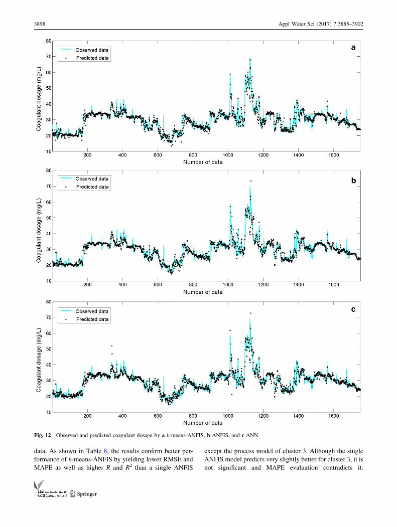
data. As shown in Table 8, the results confirm better per-

formance of k-means-ANFIS by yielding lower RMSE and

MAPE as well as higher R and R2 than a single ANFIS

except the process model of cluster 3. Although the single

ANFIS model predicts very slightly better for cluster 3, it is

not significant and MAPE evaluation contradicts it.

Fig. 12 Observed and predicted coagulant dosage by a k-means-ANFIS, b ANFIS, and c ANN

3898 Appl Water Sci (2017) 7:3885–3902

123

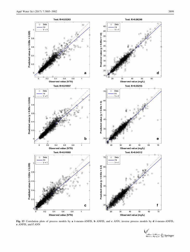
Fig. 13 Correlation plots of process models by a k-means-ANFIS, b ANFIS, and c ANN; inverse process models by d k-means-ANFIS,

e ANFIS, and f ANN

Appl Water Sci (2017) 7:3885–3902 3899

123

Especially, both models of cluster 1 & 2 show significantly

improved performances. As illustrated in Fig. 10, it can be

noticed that the MFs of k-means-ANFIS spread more

widely in the entire range than MFs of single ANFIS.

Table 9 gives comparative analysis of the completed k-

means-ANFIS models, combining together three sub-

models of process and inverse process, respectively, with

ANFIS and ANN models.

According to the results, all models satisfy the evalua-

tion criteria as good models: R[ 0.8, R2[ 0.8, R2m [ 0.5.

However, as shown in Table 9, k-means-ANFIS model

provides better prediction results than ANFIS and ANN

models for all evaluation criteria. Therefore, k-means-

ANFIS method can be effectively applied to the process

and the inverse process models of coagulation. The results

of three models in the test phase are graphically compared

by the plots of both observed and predicted values

(Figs. 11, 12, 13).

The comparison of method proposed in this research

with the existing methods from several literatures on

coagulation modeling is presented in Table 10. Zhang and

Stanley obtained good result with R2 value of 0.95 for

inverse process model; however, the model was built based

on only good cases of effluent turbidity and not covering all

seasonal variations. The good performances of the models

by Maier et al. resulted from small number of bench scale

data. However, the model derived from bench scale data is

generally unable to account for the simultaneous change in

key process parameters, and often fail when applied to real

WTP (Baxter et al. 1999). Robenson et al. made an accu-

rate model using 11 inputs, but it could not catch up with

the proposed model’s performance even though they used

time series of coagulant dosage as input parameters. Ken-

nedy et al. built an acceptable model with the R value of

0.91; however, it was caused by daily sampling and rela-

tively stable raw water quality, such as turbidity from 1.9 to

37.7 NTU. Therefore, it has a limitation of real-time pre-

dictions under abrupt large changes of raw water quality.

The seasonal models by Griffiths and Andrews were built

under similar simulation conditions to this work, but the

overall performances of the seasonal models are lower than

k-means-ANFIS models despite using more inputs. The

results in this section demonstrate that k-means-ANFIS

models are superior to those in the literatures under the

condition when real-time predicting is required for WTP

which has big fluctuation of raw water quality throughout a

year.

Conclusions

In this research, hybrid of k-means-ANFIS method was

proposed and applied to predict the settled water turbidity

and the optimal coagulant dosage with full-scale data from

Bansong WTP (South Korea). The general ANFIS and

ANN models were implemented for comparison as well. k-

means clustering successfully characterized the wide-range

influent conditions into four distinct groups. Then, four

sub-models representing different process states of raw

water quality were developed and merged into three sub-

models. The evaluation results demonstrated high perfor-

mance of the hybrid approach of k-means clustering and

ANFIS. On the whole, the sub-models of k-means-ANFIS

performed better than a single ANFIS model, especially it

Table 10 Summary of process and inverse process ANN models on coagulation in the literatures

Literature Number of inputs Data samples R2 (R) Model

The proposed method 5 FS, 1[h], 8755 0.87 (0.93) Process

5 0.93 (0.96) Inverse process

Zhang and Stanley (1999) 10 FS, 1745 0.24 Process

10 0.95 Inverse process

Maier et al. (2004) 7 BS, 202 0.90 Process

9 0.94 Inverse process

Robenson et al. (2009) 11 FS 0.95 Inverse process

Griffiths and Andrews (2011a) 12 FS, 1[h] 0.79 Process (fall)

10 0.71 Process (spring)

10 0.63 Process (winter)

12 0.89 Inverse process (fall)

10 0.82 Inverse process (spring)

10 0.78 Inverse process (winter)

Kennedy et al. (2015) 9 FS, 24[h] (0.91) Process

MAE mean absolute error, FS full scale, BS bench scale

3900 Appl Water Sci (2017) 7:3885–3902

123

could achieve the most improved prediction results for

cluster 1 & 2 models occupying rainy season. The pre-

diction improvement of rainy season in R2 index was

21.2% for the process model and 12.6% for the inverse

process model. It indicates that k-means-ANFIS models

can be used as a robust tool during rainy season which is

the most challenging period of operation. In comparison

with the general ANFIS and ANN, k-means-ANFIS also

provided the best results in all evaluation indices: RMSE,

MAPE, R, R2, R2m. Therefore, the proposed hybrid approach

can be used effectively for modeling the process and the

inverse process of coagulation. It can provide operators

with effective decision supports on both water quality

control and operational costs.

Acknowledgements The authors would like to thank the staffs who

are working at Basnong water treatment plant in Changwon city,

South Korea for supporting the data in this research.

Open Access This article is distributed under the terms of the

Creative Commons Attribution 4.0 International License (http://

creativecommons.org/licenses/by/4.0/), which permits unrestricted

use, distribution, and reproduction in any medium, provided you give

appropriate credit to the original author(s) and the source, provide a

link to the Creative Commons license, and indicate if changes were

made.

References

Abbas OA (2008) Comparisons between data clustering algorithms.

Int Arab J Inf Technol 5(3):320–325

Aguado D, Montoya T, Borras L et al (2008) Using SOM and PCA

for analyzing and interpreting data from a P-removal SBR. Eng

Appl Artif Intell 21:919–930

Al-Abadi AM (2014) Modeling of stage-discharge relationship for

Gharraf River, southern Iraq using backpropagation artificial

neural networks, M5 decision trees, and Takagi–Sugeno infer-

ence system technique: a comparative study. Appl Water Sci.

doi:10.1007/s13201-014-0258-7

Baxter CW, Stanley SJ, Zhang Q (1999) Development of a full-scale

artificial neural network model for the removal of natural organic

matter by enhanced coagulation. Water Supply Res Technol

Aqua 48(4):129–136

Baxter CW, Tupas RRT, Zhang Q et al (2001a) Artificial intelligence

systems for water treatment plant optimization. American Water

Works Association Research Foundation and American Water

Works Association, Denver

Baxter CW, Zhang Q, Stanley SJ et al (2001b) Drinking water quality

and treatment: the use of artificial neural networks. Can J Civ

Eng 28(1):26–35

Baxter CW, Stanley SJ, Zhang Q et al (2002) Development artificial

neural network models of water treatment processes: a guide for

utilities. J Environ Sci 1(3):201–211

Chen WB, Liu WC (2014) Artificial neural network modeling of

dissolved oxygen in reservoir. Environ Monit Assess

186:1203–1217

Chiu SL (1994) Fuzzy model identification based on cluster

estimation. J Intell Fuzzy Syst 2(3):267–278

Davies DL, Bouldin DW (1979) A cluster separation measure. IEEE

Trans Pattern Anal Mach Intell PAMI 1(2):224–227

Gagnon C, Grandjean BPA, Thibault J (1997) Modelling of coagulant

dosage in a water treatment plant. Artif Intell Eng 11(4):401–404

Griffiths KA, Andrews RC (2011a) The application of artificial neural

networks for the optimization of coagulant dosage. Water Sci

Technol Water Supply 11(5):605–611

Griffiths KA, Andrews RC (2011b) Application of artificial neural

networks for filtration optimization. J Environ Eng

137(11):1040–1047

Hagan MT, Menhaj MB (1994) Training feedforward networks with

the marquardt algorithm. IEEE Trans Neural Netw 5(6):989–993

Haykin S (1998) Neural networks: a comprehensive foundation, 2nd

edn. Prentice-Hall, New York, pp 26–32

Heddam S, Bermad A, Dechemi N (2012) ANFIS-based modeling for

coagulant dosage in drinking water treatment plant: a case study.

Environ Monit Assess 184(4):1953–1971

Jang JSR (1993) ANFIS: adaptive-network-based fuzzy inference

system. IEEE Trans Syst Man Cybern 23(3):665–685

Juntunen P, Liukkonen M, Lehtola M et al (2013) Cluster analysis by

self-organizing maps: an application to the modelling of water

quality in a treatment process. Appl Soft Comput 13:3191–3196

Kennedy MJ, Gandomia AH, Miller CM (2015) Coagulation mod-

eling using artificial neural networks to predict both turbidity and

DOM-PARAFAC component removal. J Environ Chem Eng

3(4):2829–2838

MacQueen J (1967) Some methods for classification and analysis of

multivariate observations. In: Proceedings of fifth Berkeley

symposium on mathematical statistics and probability, vol I.

Statistics, Berkeley and Los Angeles, University of California

Press, pp 281–297

Maier HR, Morgan N, Chow CWK (2004) Use of artificial neural

networks for predicting optimal alum doses and treated water

quality parameters. Environ Model Softw 19(5):485–494

Michael N (2005) Artificial intelligence: a guide to intelligent

systems, 2nd edn. Addison-Wesley, New York, p 276

Mohamad IB, Usman D (2013) Standardization and its effects on k-

means clustering algorithm. Res J Appl Sci Eng Technol

6(17):3299–3303

Mondal SK, Jana S, Majumder M et al (2012) A comparative study

for prediction of direct runoff for a river basin using geomor-

phological approach and artificial neural networks. Appl Water

Sci. doi:10.1007/s13201-011-0020-3

Mooi E, Sarstedt M (2011) A concise guide to market research: the

process, data, and methods using IBM SPSS statistics. Springer,

Berlin, pp 237–284

Park S, Bae H, Kim C (2008) Decision model for coagulant dosage

using genetic programming and multivariate statistical analysis

for coagulation/flocculation at water treatment process. Korean J

Chem Eng 25(6):1372–1376

Robenson A, Abd.Shukor SR, Aziz N (2009) Development of process

inverse neural network model to determine the required alum

dosage at Segama water treatment plant Sabah, Malaysia. In:

10th international symposium on process systems engineering:

part A, pp 525–530

Rousseeuw PJ (1987) Silhouettes: a graphical aid to the interpretation

and validation of cluster analysis. J Comput Appl Math

20(1):53–65

Roy PP, Roy K (2008) On some aspects of variable selection for

partial least squares regression models. QSAR Comb Sci

27(3):302–313

Sahoo AK, Zuo MJ, Tiwari MK (2012) A data clustering algorithm

for stratified data partitioning in artificial neural network. Expert

Syst Appl 39(8):7004–7014

Appl Water Sci (2017) 7:3885–3902 3901

123

Shu C, Ouarda TBMJ (2008) Regional flood frequency analysis at

ungauged sites using the adaptive neuro-fuzzy inference system.

J Hydrol 349:31–43

Takagi T, Sugeno M (1985) Fuzzy identification of systems and its

applications to modeling and control. IEEE Trans Syst Man

Cybern 15(1):116–132

Talebizadeh M, Moridnejad A (2011) Uncertainty analysis for the

forecast of lake level fluctuations using ensembles of ANN and

ANFIS models. Expert Syst Appl 38(4):4126–4135

Weigend AS, Rumelhart DE, Huberman BA (1990) Predicting the

future: a connectionist approach. Int J Neural Syst 1(3):193–209

Wu GD, Lo SL (2008) Predicting real-time coagulant dosage in water

treatment by artificial neural networks and adaptive network-

based fuzzy inference system. Eng Appl Artif Intell

21(8):1189–1195

Yu RF, Kang SF, Liaw SL et al (2000) Application of artificial neural

network to control the coagulant dosing in water treatment plant.

Water Sci Technol 42(3–4):403–408

Zhang Q, Stanley SJ (1999) Real-time water treatment process control

with artificial neural networks. J Environ Eng 125(2):153–160

Zhu J, Segovia J, Anderson P (2015) Defining influent scenarios:

application of cluster analysis to a water reclamation plant.

J Environ Eng 141(7):04015005

3902 Appl Water Sci (2017) 7:3885–3902

123