Work ing PaPer Ser ieSno 1537 / aPr i l 2013

Prediction USing Several MacroeconoMic ModelS

Gianni Amisano and John Geweke

In 2013 all ECB publications

feature a motif taken from

the €5 banknote.

note: This Working Paper should not be reported as representing the views of the European Central Bank (ECB). The views expressed are those of the authors and do not necessarily reflect those of the ECB.

© European Central Bank, 2013

Address Kaiserstrasse 29, 60311 Frankfurt am Main, GermanyPostal address Postfach 16 03 19, 60066 Frankfurt am Main, GermanyTelephone +49 69 1344 0Internet http://www.ecb.europa.euFax +49 69 1344 6000

All rights reserved.

ISSN 1725-2806 (online)EU Catalogue No QB-AR-13-034-EN-N (online)

Any reproduction, publication and reprint in the form of a different publication, whether printed or produced electronically, in whole or in part, is permitted only with the explicit written authorisation of the ECB or the authors.This paper can be downloaded without charge from http://www.ecb.europa.eu or from the Social Science Research Network electronic library at http://ssrn.com/abstract_id=2252579.Information on all of the papers published in the ECB Working Paper Series can be found on the ECB’s website, http://www.ecb.europa.eu/pub/scientific/wps/date/html/index.en.html

Acknowledgements A report on some aspects of this work using a different data set appears as Geweke and Amisano (2012a).The views expressed do not represent those of the ECB. Much of Amisano’s work was carried out while on secondment (ECB “External Working Experience” program) at UTS. Amisano thanks UTS for providing warm hospitality, a very stimulating working environment and excellent computing facilities.Geweke acknowledges partial nancial support from Australian Research Council grant DP110104372.

Gianni AmisanoEuropean Central Bank; e-mail: gianni.amisano@ecb.europa.eu

John GewekeUniversity of Technology Sydney, Erasmus University and University of Colorado; e-mail: john.geweke@uts.edu.au

Abstract

Prediction of macroeconomic aggregates is one of the primary functions ofmacroeconometric models, including dynamic factor models, dynamic stochasticgeneral equilibrium models, and vector autoregressions. This study establishesmethods that improve the predictions of these models, using a representative modelfrom each class and a canonical 7-variable postwar US data set. It focuses on pre-diction over the period 1966 through 2011. It measures the quality of predictionby the probability densities assigned to the actual values of these variables, onequarter ahead, by the predictive distributions of the models in real time. Twosteps lead to substantial improvement. The �rst is to use full Bayesian predictivedistributions rather than substitute a �plug-in� posterior mode for parameters.Across models and quarters, this leads to a mean improvement in probability of50.4%. The second is to use an equally-weighted pool of predictive densities fromthe three models, which leads to a mean improvement in probability of 41.9%over the full Bayesian predictive distributions of the individual models. This im-provement is much better than that a¤orded by Bayesian model averaging. Thestudy uses several analytical tools, including pooling, analysis of predictive vari-ance, and probability integral transform tests, to understand and interpret theimprovements.

1

Keywords: Analysis of variance, Bayesian model averaging, dynamic factor model, dynamic stochastic general equilibrium model, prediction pools, probability integral transform test, vector autoregression model

JEL codes: C11, C51 C53

Non-technical summaryDecision-making theory requires that the decision-maker have a coherent probability

distribution over relevant unknown magnitudes. Often these include future events, andthere are alternative approaches (or models) that the decision maker, and the decision-maker�s sta¤, can take in approaching this task. This requires that the approachessomehow be brought together in order to arrive at a single distribution.This work examines some of the ways in which this task can be addressed in the

particular case of macroeconometric models. Central banks, in particular, routinely uti-lize these models, and increasingly focus on probability distributions for future eventsas opposed to point forecasts. In many cases research departments maintain and im-prove several alternative models and bring forward their di¤erent predictions to a fairlyadvanced point in support of monetary policy.We consider alternative approaches to formulating predictive distributions frommacro-

economic models, and reconciling their implications with full allowance for the fact thatnone of the models corresponds �or even comes close �to reality. The study focuses onthree macroeconometric models: a dynamic factor model (DFM), a dynamic stochasticgeneral equilibrium (DSGE) model, and a vector autoregression (VAR) model. We haveseveral reasons for taking this approach. First, these are representatives of the three ma-jor families of macroeconometric models used for prediction in central banks. Second,these families di¤er in the ways in which they attempt to use general equilibrium theoryas a source of information in formulating the model and conducting statistical inference.Third, the models take di¤erent approaches in the marshalling of prior information thatis required if useful predictions about complex phenomena are to be constructed fromrelatively sparse data. Finally, our recent methodological work on some aspects of thisproblem (Geweke and Amisano, 2011) suggests that model combination is most fruit-ful when the models at hand are dissimilar. This is exactly what happens in portfolioallocation: diversi�cation is particularly useful when the available assets have di¤erentproperties in di¤erent states of the world.We concentrate exclusively on the same canonical US data for seven macroeconomic

aggregates used by Smets and Wouters (2007), incorporating subsequent revisions oftheir data and extending it through the last quarter of 2011.Four principal analytical tools are used in our construction and interpretation of

predictive distributions. Two are competing approaches to model combination, Bayesianmodel averaging and linear prediction pools. We use analysis of predictive variance(Geweke and Amisano, 2012b) to understand the gains from using prediction poolsand to interpret the superiority of full Bayesian predictive distributions to predictivedistributions based on point estimates that emerges in this work. The probability integraltransform tests adduce evidence that all of the models studied here are grossly unrealisticin particular dimensions. We regard this fact both as fundamental in guiding approachesto model combination for purposes of prediction and in explaining the relatively poorperformance of Bayesian model averaging in the empirical work.We study two leading methods for prediction, one based on substituting the posterior

mode for the parameter vector and the other using the full Bayesian predictive distri-

2

bution. In general �though not entirely without exception �the latter performs muchbetter than the former. It shows that these di¤erences can be traced to quarters thatturn out to be "outliers," realizations that have relatively low probability as assessed byany of the models. It shows that the e¤ect arises because parameter uncertainty is animportant source of variance in full predictive distributions that is ignored when onlyposterior modes are used. Finally, it shows that the e¤ect is smallest in the DSGE modeland strongest in the VAR model (the one with the most parameters, in which predictivevariance due to parameter uncertainty is also largest).We also pursue the combination of models for purposes of prediction using linear

combinations. The simple average of predictive distributions turns out to be very e¤ec-tive and imposes essentially no demands on the econometrician beyond those requiredto evaluate the predictive performance of the di¤erent models in the �rst place. Analternative is an optimal linear pool with weights updated at the end of each quarterto combine the model predictive densities for the next quarter. This turns out to fallsomewhat short of the equally-weighted pool. This comparison is speci�c to the threemodels used and the data employed here, and may well be attributed to the fact thatwe use three models that have all held their own in the marketplace of macroeconomicprediction. Bayesian model averaging falls well short of either pool for the entire periodstudied. The explanation is rooted in the fact that Bayesian model averaging conditionson one of the models being fully correctly speci�ed (though which one is not known apriori), a condition that is manifesting unrealistic here.

3

1 Introduction

Normative decision-making theory, based on expected utility, requires that the decision-maker have a coherent probability distribution over relevant unknownmagnitudes. Oftenthese include future events, and often there are alternative approaches that the decisionmaker, and the decision-maker�s sta¤, can take in approaching this task. This requiresthat the approaches somehow be brought together in order to arrive at a single distri-bution. While this is a rare�ed depiction of actual decision-making, in the real worldsubstantial time, e¤ort and resources are devoted to distilling the logical implications ofdisparate views of uncertainty that emerge from even the most disinterested and skillfulmodelling of the course of future events.This work examines some of the ways in which this task can be addressed in the par-

ticular case of macroeconometric models that are designed for the purpose of assigningprobabilities to the future course of principal economic aggregates. Central banks, inparticular, routinely utilize these models, and increasingly focus on probability distribu-tions for future events as opposed to point forecasts. In many cases research departmentsmaintain and improve several alternative models and bring forward their di¤erent pre-dictions to a fairly advanced point in support of monetary policy. Reconciling di¤erencesamong these models will not soon, if ever, be reduced to one formal procedure. However,there are well-de�ned steps in this direction.This work takes up some alternative approaches to formulating predictive distribu-

tions from macroeconomic models, and reconciling their implications with full allowancefor the fact that none of the models corresponds �or even comes close �to reality. Indoing this it brings together a number of analytical tools, with some re�nements beyondthose in the literature, and uses them to sort through di¤erent approaches, understandtheir di¤erences, and make practical recommendations for prediction in central banks.The study focuses on three macroeconometric models: a dynamic factor model

(DFM), a dynamic stochastic general equilibrium (DSGE) model, and a vector au-toregression (VAR) model. We have several reasons for taking this approach. First,these are representatives of the three major families of macroeconometric models usedfor prediction in central banks. Second, these families di¤er in the ways in which theyattempt to use general equilibrium theory as a source of information in formulatingthe model and conducting statistical inference. Third, the models take di¤erent ap-proaches in the marshalling of prior information that is required if useful predictionsabout complex phenomena are to be constructed from relatively sparse data. Finally,our recent methodological work on some aspects of this problem (Geweke and Amisano,2011) suggests that model combination is most fruitful when the models at hand aredissimilar.This is very similar to what is found in empirical optimal porfolio alloca-tion: diversi�cation works best when di¤erent asset categories have desirable features indi¤erent states of the world.Section 2 provides summary detail of the three models. We concentrate exclusively

on the same canonical US data for seven macroeconomic aggregates used by Smetsand Wouters (2007), incorporating subsequent revisions of their data and extending it

4

through the last quarter of 2011. The paper studies predictive performance over 184quarters, 1966 through 2011, breaking this up into three periods of interest described inSection 2. The work here is all based on probability distributions over a single-period(one quarter) horizon. Posterior distributions or modes are constructed for each sample,the �rst ending in 1965:4 and used for prediction of the seven aggregates for 1966:1, andthe last ending in 2011:3 and used for prediction of the seven aggregates for 2011:4. Inthat sense the analysis here is �out of sample,�mimicking what a real econometricianwould do in real time. However this study does not attempt to limit attention to themost recent data revisions available each quarter, nor does it grapple with the questionof which vintage of revised data should be used in assessing the predictions. The mostrecent revisions available on February 16, 2012, are used for all purposes through thepaper.Section 3 summarizes the four principal analytical tools used in our construction and

interpretation of predictive distributions from several models and alternative approachesto inference. Two are competing approaches to model combination, Bayesian model av-eraging and linear prediction pools. We use analysis of predictive variance (Geweke andAmisano, 2012b) to understand the gains from using prediction pools and to interpretthe superiority of full Bayesian predictive distributions to predictive distributions basedon point estimates that emerges in this work. The probability integral transform testsadduce evidence that all of the models studied here are grossly unrealistic in particulardimensions. We regard this fact both as fundamental in guiding approaches to modelcombination for purposes of prediction and in explaining the relatively poor performanceof Bayesian model averaging in the empirical work.The balance of the paper is devoted to the formulation, evaluation and understanding

of the predictive distributions that emerge in the three models and in di¤erent combi-nations of these distributions. Section 4 studies two leading methods for prediction, onebased on substituting the posterior mode for the parameter vector and the other usingthe full Bayesian predictive distribution. In general �though not entirely without excep-tion �the latter performs much better than the former. It shows that these di¤erencescan be traced to quarters that turn out to be �outliers,�realizations that have relativelylow probability as assessed by any of the models. It shows that the e¤ect arises becauseparameter uncertainty is an important source of variance in full predictive distributionsthat is ignored when only posterior modes are used. Finally, it shows that the e¤ectis smallest in the DSGE model (the one with the fewest parameters, in which predic-tive variance due to parameter uncertainty is also smallest) and strongest in the VARmodel (the one with the most parameters, in which predictive variance due to parameteruncertainty is also largest).For predictions of several random variables, the case considered here, a theorem

of McConway (1981) shows that the marginal distributions of a pool of multivariatepredictive densities can be identical to the same pool of marginal predictive densities ifand only if the pool is linear in the predictive densities. This motivates the requirementthat the pool be linear and renders the analysis tractable while still leaving open anumber of interesting possibilities. The simple average of predictive distributions turns

5

out to be very e¤ective and imposes essentially no demands on the econometricianbeyond those required to evaluate the predictive performance of the di¤erent modelsin the �rst place. An alternative is an optimal linear pool with weights updated atthe end of each quarter to combine the model predictive densities for the next quarter.This turns out to fall somewhat short of the equally-weighted pool. This comparison isspeci�c to the three models used and the data employed here, and may well be attributedto the fact that we use three models that have all held their own in the marketplace ofmacroeconomic prediction. Bayesian model averaging falls well short of either pool forthe entire period studied. The explanation is rooted in the fact that Bayesian modelaveraging conditions on one of the models being fully correctly speci�ed (though whichone is not known a priori), a condition that is manifestly unrealistic here.The paper concludes with a short quantitative recapitulation of the results.

2 Models and data

The models that we study are a representative selection of forecasting models used inmacroeconomic policy environments. Some models are typically speci�ed in order to in-corporate features directly drawn from economic theory. Among these models, dynamicstochastic general equilibrium models have been widely used in many central banks toproduce forecasts, historical decompositions aiming at assessing the relevance of di¤erentkinds of macroeconomic shocks, and counterfactual analyses. Smets and Wouters (2003,2007) have shown that these models can be successfully estimated with satisfactory �tand forecasting properties. Del Negro and Schorfheide (2012) provides interesting dis-cussion of how DSGE models have fared in the recent past and how external informationcan be brought to bear to improve them.On the other hand, policy-oriented macroeconomic forecasting is often based on time

series models that are more agnostic with respect to general equilibrium theory. Amongthese models, the most widely used are the vector autoregression models introduced bySims (1980). These models are characterized by a parameter space of high dimensionand typically employ prior distributions with carefully chosen hyperparameters.It is often said that economic policy requires very large amounts of economic infor-

mation being taken into consideration in order to guide decision making (Bernanke andBoivin, 2003). Dynamic factor models (Geweke, 1977; Sargent and Sims, 1977; Stockand Watson, 2002a; Forni, Hallin, Lippi and Reichlin, 2005) are well suited to this task.In these models the joint behavior of a large number of economic time series is jointlymodelled by specifying that the series are driven by a small set of persistent commonfactors and by idiosyncratic shocks.The strategy of combining di¤erent macroeconomic models with each other and with

information beyond the data, pursued in this paper, is well-established in the macroeco-nomic prediction literature. One approach, re�ected in the models we use, is to enrichthe statistical structure of disturbances. Sargent (1989) and Ireland (2004) incorporatedmeasurement errors to avoid stochastic singularity. Canova (2008) added measurement

6

errors to relax the implications of a DSGE model for the low frequency properties ofthe time series. Smets and Wouters (2007) incorporated serial correlation in shocks toimprove the predictions of DSGE models.Combining models of the kind used here is another theme in this literature. The �rst

attempt in this direction appears to be Ingram and Whiteman (1994), who linearizedthe mapping between DSGE and VAR parameters and then employed the prior for VARparameters implied by a normal prior distribution for DSGE model parameters. DelNegro and Schorfheide (2004) provided a hierarchical prior distribution in which DSGEmodel restrictions enter a VAR with noise. Schorfheide et al. (2011) utilized the sameapproach using a DFM rather than a VAR model. Waggoner and Zha (2012) build a fullmixture of a DSGE and VAR model. We are not aware of previous work that combinesDSGE, VAR and DFM models simultaneously.All these considerations lead us to include in our analysis three speci�c models rep-

resentative of these classes, referred to subsequently as DFM, DSGE and VAR, in orderto provide a compact, yet representative, basis to span the model set commonly used inan economic policy environment. Going forward, in circumstances where the ordering ofthe models is arbitrary, we refer to these models in alphabetical order of their acronyms.

2.1 Three models

The observable time series of interest in each of the three models are the log growthrates of real consumption, investment, income (GDP), and wages; the logarithm of aper capita weekly hours worked index, in�ation as measured by the growth rate of theGDP de�ator, and the nominal Federal Funds rate. In the DFM and DSGE models the�rst series appear in exactly this form. We examine two variants of VAR models: inthe VARD (VAR-di¤erences) model the series also appear in this form; in the VARL(VAR-levels) the �rst four series appear as log-levels rather than growth rates.

2.1.1 The DFM

In a dynamic factor model a set of time series is driven by a typically small set ofcommon factors and by idiosyncratic shocks. When the number of series being jointlyconsidered is high, usually non-parametric estimation is used. In this regard, Stock andWatson (2002b) and Forni, Hallin, Lippi and Reichlin (2005) show how to use staticand dynamic principal components methods to obtain consistent estimates of the spacespanned by common factors.In this study, we use a very small dynamic factor model, with a set of n = 12 variables

that includes the 7 series common to all three models. The set of additional variablesis chosen to consider, in a highly stylized way, some economic phenomena which areneglected by the information set used to estimate the DSGE and VAR models. Theseadditional variables are stock returns, the term structure slope, the risk premium, theunemployment rate and the rate of change of the money supply M2.

7

With such a compact information set, inference can be entirely parametric and weemploy the model of Stock and Watson (2005) as follows for the n � 1 vector of timeseries yt,

yt = �ft + vt, ft = c+pXj=1

Ajft�j + �t, vt =qXj=1

Bjvt�j + "t,

where ft is a k�1 vector of latent factors and vt is an n�1 vector of mutually independentidiosyncratic shocks.The parameters are subject to several restrictions. For identi�cation of factors, ij =

0 (j > i) and therefore there are r = nk � k (k � 1) =2 free parameters of the matrix� that can be collected in an r � 1 vector . Because the idiosyncratic shocks areindependent Bj = diag (bj) (j = 1; : : : ; q).The shocks are Gaussian and independent:�

�t"t

�iids N

��00

�;

�Ik 00 H�1

��.

The prior distribution has �ve independent components:

s N (0; 10 � Ir) ;c s N (0; 10 � In)

vec (Aj)iids N (0; Ik) (j = 1; : : : ; p) ;

bjiids N (0; In) (j = 1; : : : ; q) ;

0:4 � hiiids �2 (4) (i = 1; : : : ; n) .

After preliminary investigations to settle on a satisfactory speci�cation, we chosek = 3 common factors, VAR dynamics of order p = 2, and idiosyncratic shock dynamicsof order q = 2. The total number of parameters in the model is r+n+pk2+nq+n = 99.The linear-Gaussian state space nature of the model easily lends itself to Gibbs

sampling with data augmentation. The conditional distributions of (a1; : : : ; ap) and(b1; : : : ; bq) require a Metropolis-Hastings within Gibbs approach, while the conditionaldistributions of and (h1; : : : ; hn) are known analytically; the simulation of the latentcommon factors is straightforward. For each of the subsamples being analyzed, werun 65,000 MCMC iterations, after 15,000 burn-in draws to ensure convergence of thealgorithm. The MCMC output was thinned to 10,000 recorded draws to save on storagespace. We also computed posterior modal values for the parameters by using the Gibbs-based simulated annealing algorithm proposed by Doucet, Godsill and Robert (2002).

2.1.2 The DSGE model

The dynamic stochastic general equilibrium model we use in this study is exactly themodel described in Smets and Wouters (2007), which details and discusses the model�s

8

speci�cation. To brie�y summarize the model�s main characteristics, we just recallthat the model has two sectors, intermediate goods and �nal goods. The �rst sectorproduces di¤erentiated goods in a monopolistically competitive setting, while the secondsector is perfectly competitive. Both wages and prices are sticky and the in�nitely-livedrepresentative consumer has utility characterized by consumption habits. Monetarypolicy is speci�ed as a Taylor rule and real variables are all characterized by a commondeterministic growth rate which is estimated with all the other parameters of the model.The model has seven shocks: an aggregate total factor productivity shock, an investmentspeci�c shock, a risk premium shock (which acts as proxy for �nancial disturbances),wage and price mark-up shocks and �scal and monetary policy shocks.The model has 39 free parameters which we endow with exactly the same prior

structure as in Smets and Wouters (2007). We carry out Bayesian and posterior modeestimation by using the linearized solution and, as customary in the applied DSGE liter-ature (An and Schorfheide, 2007), we use a random walk Metropolis-Hastings algorithmwith candidate tailored using the Hessian of the log posterior computed at its mode. Foreach posterior, the mode is found using numerical optimization. The results obtainedare based on 40,000 MCMC draws for each subsample, after 12,000 burn-in iterations.For each of the subsamples we thin the draws to 10,000.

2.1.3 The VAR model

In the VAR the conditional distribution of the series takes the form of a normal mul-tivariate regression model in which the covariates consist of an intercept term and the�rst four lagged values of each series. Thus the model has 29 coe¢ cients in each of7 equations, making a total of 231 parameters together with the conditional variancematrix.For both the di¤erenced (VARD) and levels (VARL) variants of this model we uti-

lize the �Minnesota prior�distribution (Litterman, 1986) in which the coe¢ cients areGaussian and independent and their variances are functions of a small number of hy-perparameters. In the equation for variable i, let ci denote the intercept and aij;h thecoe¢ cient of variable j, lag h. The prior variances of these parameters are

var(aij;h) =

8<:��1 � ��h3 � �ii

�jj

�2(i = j)�

�1 � �2 � ��h3 � �ii�jj

�2(i 6= j)

var(ci) = (�1 � �4)2 ,

with �1 = :2; �2 = :9; �3 = 1; �4 = 1: In this prior distribution E (aij;h) = 0 in for allcoe¢ cients, except that E (aii;1) = 1 if variable i appears in levels. Hence, in the VARLvariant all coe¢ cients pertaining to own �rst lag have mean 1, while in the VARD variantonly hours, in�ation and the short term interest rate have own �rst lag coe¢ cient withprior variance equal to one and the other four variables have �rst own lag coe¢ cientprior mean equal to zero.

9

As regard the shocks precision matrix H; we speci�ed a Wishart distribution withparameters � = 9 and S set to match the OLS estimate ofH based on the �rst subsample.The posterior simulation of the model is based on a straightforward two block Gibbs

algorithm. For each of the subsamples analyzed, we obtained 65,000 draws, the �rst15,000 of which were discarded and the remaining 50,000 were thinned to produce 10,000retained draws.The posterior mode estimates were obtained by analytically marginalizing the joint

posterior distribution with respect to the coe¢ cients aij;h and ci. The resulting marginalposterior of H was numerically optimized yielding a modal value for H. With the modalvalue of H in hand, it is immediate to �nd the modal values of the coe¢ cients aij;h andci, because their conditional posterior distribution is Gaussian with known moments.

2.2 Data and periods of interest

The series we use for the DSGE and VAR models are exactly those described in Smetsand Wouters (2007), extended through 2011 and incorporating the latest available revi-sions. The DFM utilizes �ve additional series: stock returns, de�ned as the log di¤er-ences of quarterly averages of S&P 500 Composite index; the aggregate civilian unem-ployment rate; the term premium, measured as the di¤erence between the yields on tenyear and three month US Treasury bond; the risk premium, measured as the di¤erencebetween the Risk premium: BAA and AAA corporate bond spread; and the growth ratein the money supply M2.The relevant series were all obtained from the Federal Reserve Bank of St. Louis Data

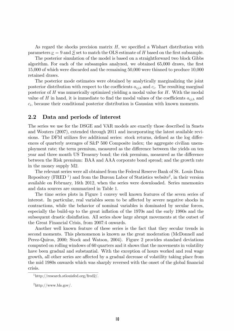
Repository (FRED 1) and from the Bureau Labor of Statistics website2, in their versionavailable on February, 16th 2012, when the series were downloaded. Series mnemonicsand data sources are summarized in Table 1.The time series plots in Figure 1 convey well known features of the seven series of

interest. In particular, real variables seem to be a¤ected by severe negative shocks incontractions, while the behavior of nominal variables is dominated by secular forces,especially the build-up to the great in�ation of the 1970s and the early 1980s and thesubsequent drastic disin�ation. All series show large abrupt movements at the outset ofthe Great Financial Crisis, from 2007:4 onwards.Another well known feature of these series is the fact that they secular trends in

second moments. This phenomenon is known as the great moderation (McDonnell andPerez-Quiros, 2000; Stock and Watson, 2004). Figure 2 provides standard deviationscomputed on rolling windows of 60 quarters and it shows that the movements in volatilityhave been gradual and substantial. With the exception of hours worked and real wagegrowth, all other series are a¤ected by a gradual decrease of volatility taking place fromthe mid 1980s onwards which was sharply reversed with the onset of the global �nancialcrisis.

1http://research.stlouisfed.org/fred2/.

2http://www.bls.gov/.

10

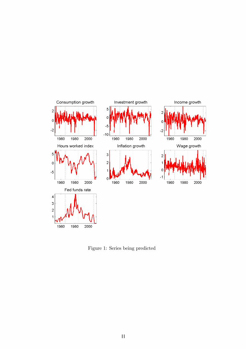
Figure 1: Series being predicted

11

Figure 2: Standard deviations of the series being predicted. Computations based onrolling window of 60 observations

12

Table 1: Data sourcesSeries Mnemonics De�nition SourceAAA Moody�s Seasoned AAA Corporate Bond Yield FREDBBB Moody�s Seasoned BAA Corporate Bond Yield FREDCE16OV Civilian Employment FREDFEDFUNDS E¤ective Federal Funds Rate FREDFPI Fixed Private Investment FREDGDPC96 Real Gross Domestic Product, 3 Decimal FREDGDPDEF Gross Domestic Product: Implicit Price De�ator FREDGS10 10-Year Treasury Constant Maturity Rate FREDLNS10000000 Civilian noninstutitional population BLSM2SL M2 stock FRED(*)PCEC Personal Consumption Expenditures FREDPRS85006023 Nonfarm Business Sector: Average Weekly Hours BLSPRS85006103 Nonfarm Business Hourly Compensation BLSSP500C SP500 composite index FREDUNRATE Civilian unemployment rate FRED(*) Prior to 1959 the M2 series comes from Balke and Gordon (1986)

This phenomenon can be alternatively described by computing standard deviationsbased on sub-samples, as we do in Table 2.The analysis that follows distinguishes among four periods:

1. Initial: 1951:1-1965:4, used to initialize the estimation of each of the models andnot used for forecasting evaluation;

2. Pre moderation: 1966:1 - 1984:4, characterized by higher volatility;

3. Great moderation: 1985:1-2007:4, characterized by smaller volatility;

4. Post moderation: 2008:1-2011:4, characterized by a return to higher volatility.

Throughout the paper t indexes quarters, with t = 1 being the �rst quarter predicted,1966:1, and t = T = 184 being the last quarter predicted, 2011:4. We denote the 7� 1vector of random variables of interest Yt, and their realized values (the data) yt. Eachmodel speci�es conditional densities p (Yt j Y1:t�1; �i; Ai) and a prior density p (�i j Ai),where Ai denotes the speci�cation of model i together with the data in the initial periodand �i is the parameter vector in model Ai. In the interest of non over-burdeningthe reader with pedantry, this abuses the notation somewhat: the conditioning dataset always goes back to 1951:1; and, in the DFM, the conditioning data includes thehistories of the �ve additional series from 1951:1 through quarter t� 1.In particular, note that all series volatilities dropped during the great moderation and

for many series volatility returned to pre moderation levels (or higher) post moderation.

13

Table 2: Standard deviations of observed data computed on di¤erent subsamplesPeriod

Pre Great PostSeries Initial moderation moderation moderationConsumption growth 0.94 0.82 0.51 1.04Investment growth 2.82 2.72 1.63 3.88

Income growth 1.16 1.09 0.53 0.97Hours worked index 2.18 3.06 1.95 3.10

In�ation 0.52 0.58 0.24 0.26Wage growth 0.56 0.49 0.67 0.75Fed funds rate 0.23 0.89 0.54 0.24

Notice also that the federal funds rate was characterized by very low volatility in theyears before 1970 and that the most recent years have reduced its volatility to the pre-1970s levels. This re�ects the very expansive monetary policy pursued by the Fed as aconsequence of the Great Financial Crisis.

3 Analytical methods

This work uses an eclectic methodology in order to understand the performance ofmacroeconometric models in prediction and to examine how an econometrician mightbest use the models at her disposal to form predictive distributions. With the exceptionof one technique discussed in Section 3.4, all of these methods appear in the literature.The treatment here is short, intended to establish notation and indicate precisely thetools used in Sections 4 and 5.

3.1 Bayesian model averaging

Bayesian model averaging is implied by the M-closed perspective of fully subjectiveBayesian inference (Bernardo and Smith, 1993, Section 6.1.2). This approach conditionson a set of models A1; : : : ; An, each with a parameter vector �i 2 �i, a prior densityp (�i j Ai), and a speci�cation of conditional densities p (Yt j Y1:t�1; �i; Ai) for a commonset of observable vectors Y1:T = fY1; : : : ; YTg. (Upper case Y denotes random vectorsand lower case y the corresponding realizations.) Model prior probabilities p (Ai), withPn

i=1 p (Ai) = 1, place models, parameter vectors and observables in a common proba-bility space.The laws of probability then imply the sequence of one-step-ahead predictive densities

p (Yt j y1:t�1) =nXi=1

p (Ai j y1:t�1) � p (Yt j y1:t�1; Ai) .

14

The model predictive densities

p (Yt j y1:t�1; Ai) =Z�i

p (Yt j y1:t�1; �i; Ai) p (�i j y1:t�1; Ai) d�i (t = 1; : : : ; T ) (1)

are accessed as described in Section 2.1. The conditional probabilities p (Ai j y1:t�1), alsoknown as Bayesian model averaging weights, are

p (Ai j y1:t�1) / p (Ai) p (y1:t�1 j Ai) = p (Ai)t�1Ys=1

p (ys j y1:s�1; Ai) . (2)

The marginal likelihoods p (ys j y1:s�1; Ai) are evaluated as described in Section 2.1.Given weak regularity conditions, including the existence of a true data generating

process p (Yt j Y1:t�1; D),

t�1tXs=1

log p (Ys j Y1:s�1; Ai)a:s:�! LSi

as detailed in Geweke and Amisano (2011). So long as j = argmaxi (LSi) is uniquep (Aj j Y1:t�1)

a:s:�! 1, and p (Ai j Y1:t�1)a:s:�! 0 for i 6= j. If in fact Ak = D for some

k 2 f1; : : : :ng then j = k.

3.2 Pooling

Suppose that R1; : : : ; Rn are prediction rules, each specifying a sequence of predictivedensities p (Yt; y1:t�1; Ri) (t = 1; : : : ; T ). A prediction rule Ri could coincide with a se-quence of model predictive densities (1), but it might also be any sequence of legitimatepredictive densities that depends only on information actually available at t � 1. Forexample it could be the sequence

p�Yt j y1:t�1;b�i (t� 1) ; Ai� (t = 1; : : : ; T ) (3)

where b�i (t� 1) = argmax�ip (�i j Ai) p (y1:t�1 j �i; Ai) , (4)

the posterior mode.A linear pool of n prediction rules R1; : : : ; Rn is the sequence of predictive densities

p (Yt; y1:t�1;wt�1; R1; : : : ; Rn) =

nXi=1

wt�1;ip (Yt; y1:t�1; Ri) (t = 1; : : : ; T ) (5)

wherewt�1 is a point in the n-dimensional unit simplex, i.e. wt�1;i � 0 (i = 1; : : : ; n) andPni=1wt�1;i = 1. The subscript t � 1 indicates the requirement that wt�1 also depends

15

only on information actually available at t�1. Arguably the simplest pool is the equallyweighted pool (EWP) that speci�es wt�1;i = n�1 (t = 1; : : : ; T ; i = 1; : : : ; n).Any prediction ruleR formed at time t can be evaluated using the log scoring criterion

tXs=1

log p (ys; y1:s�1; R) . (6)

There are several compelling arguments for this rule, summarized in Geweke and Amisano(2011). Note that if p (yt j y1:t�1; R) = p (yt j y1:t�1; Ai) (t = 1; : : : ; T ), the sequence ofpredictive likelihoods for model Ai, then the criterion (6) is the log marginal likelihoodlog p (y1:t j Ai). An optimal prediction pool selects w�

t�1 to maximize this criterion:

w�t�1 = argmax

wt�1

t�1Xs=1

log

"nXi=1

wt�1;ip (ys; y1:s�1; Ri)

#.

subject to the constraint that wt�1 be in the n-dimensional unit simplex. This is asimple convex programming problem.This process generates a sequence of weight vectors and corresponding pools, each of

which we refer to subsequently as a real-time optimal pool (RTOP). Because wt�1 andp (yt�1; y1:t�2; Ri) involve only information actually available at the end of period t� 1,this mimics a procedure that could have been carried out by an econometrician in realtime. In order to summarize the behavior of pools over various time intervals, we shallsometimes refer to static optimal pools of the form

w�r:t = argmax

w

tXs=r

log

"nXi=1

wip (ys; y1:s�1; Ri)

#(7)

for particular choices of r and t. Note that w�1:t�1 = w�

t�1. The log score of a staticoptimal pool cannot be less (and is generally greater) than the log score of the corre-sponding equally weighted pool. The log score of a RTOP can be less than that of thecorresponding equally weighted pool.

3.3 Analysis of predictive variance

The variance implicit in a Bayesian predictive distribution can be decomposed intoseveral sources as described in Geweke and Amisano (2012b). The approach provesuseful here in understanding the relative performance of two popular approaches toforming predictive densities in macroeconometric models, the fully Bayesian predictivedistribution with the sequence of densities (1) and the posterior mode or �plug in�approach (3). Due to the particular characteristics of predictive distributions in thethree models, discussed in Section 2.1, the technical steps di¤er from those in Gewekeand Amisano (2012b) and are somewhat simpler.

16

Consider �rst the predictive distributions for a single model Ai. By the law of totalprobability

var (Yt j y1:t�1; Ai) = E�i f[var(Yt j y1:t�1; �i; Ai)] j y1:t�1; Aig+var�i f[E(Yt j y1:t�1; �i; Ai)] j y1:t�1; Aig . (8)

Following Geweke and Amisano (2012b), the �rst term on the right side of (8) is theintrinsic variance of the predictive distribution, so named because it is the variance inthe predictive distribution that would exist even if �i were known, averaged over thedistribution of �i speci�ed in the relevant posterior distribution. The second term onthe right side of (8) is the extrinsic variance of the predictive distribution, so namedbecause it is the variance in the conditional mean that arises from the fact that �i is notdegenerate in the relevant posterior distribution.As detailed in Section 2.1, the distribution

Yt j (y1:t�1; �i; Ai) s N [� (y1:t�1; �i) ; V (y1:t�1; �i)]

in all of the macroeconometric models considered in this work. The vector � (y1:t�1; �i)and matrix V (y1:t�1; �i) have closed form expressions that are easy to evaluate. Corre-sponding to the vectors �(m)t�1;i (m = 1; : : : ;M) from the posterior simulator for model Aiand the sample y1:t�1, let

�(m)t�1;i = �

�y1:t�1; �

(m)t�1;i

�; V

(m)t�1;i = V

�y1:t�1; �

(m)t�1;i

�(t = 1; : : : ; T � 1; i = 1; : : : ; n;m = 1; : : : ;M), and

�t�1;i =M�1

MXm=1

�(m)t�1;i (t = 1; : : : ; T � 1; i = 1; : : : ; n) .

Then the relevant numerical approximations in (8) are

E�i f[var (Yt j y1:t�1; �i)] j y1:t�1; Aig uM�1MXm=1

V(m)t�1;i = V It�1;i (9)

for intrinsic variance and

var�i f[E (Yt j y1:t�1; �i)] j y1:t�1; Aig

u (M � 1)�1MXm�1

h�(m)t�1;i � �t�1;i

i h�(m)t�1;i � �t�1;i

i0= V Et�1;i (10)

for extrinsic variance (t = 1; : : : ; T � 1; i = 1; : : : ; n). The approximation of total vari-ance is the sum of (9) and (10). Then the fraction of the variance that is extrinsic may

17

be computed in the obvious way for each component of Yt, using the diagonal elementsof V It�1;i andV Eti�1;i.For any pool with weight vector w this analysis can be extended to remove the con-

ditioning on model Ai. From Geweke and Amisano (2012b, Proposition 4) the governinglaw of total probability is

var (Yt j y1:t�1) = EAi;�i f[var (Yt j y1:t�1; �i; Ai)] j y1:t�1g+EAi hvar�i f[E (Yt j y1:t�1; �i)] j y1:t�1; Aig j y1:t�1i+varAi [E (Yt+1 j y1:t�1; Ai) jy1:t�1] : (11)

The �rst term on the right side of (11) is the intrinsic variance, and its numerical approx-imation is

Pni=1wiV

intt�1;i. The second term is the within-model extrinsic variance, and its

numerical approximation isPn

i=1wiVextt�1;i. The last term is the between-model extrinsic

variance, and its numerical approximation isPn

i=1wi��it�1 � �t�1

� ��it�1 � �t�1

�0where

�t�1 =Pn

i=1wi�it�1.

In the applications in this work the original posterior simulation samples of size10,000 are thinned to simulation samples of sizeM = 1; 000, which becomes the relevantsimulation sample for the approximations just described.

3.4 Model evaluation with probability integral transforms

A data generating process D for a vector time series Yt implies conditional cumulativedistribution functions for any element Yjt of Yt,

Fj (x;Y1:t�1;D) = P (Yjt � x j Y1:t�1; D) :

Rosenblatt (1952) showed that the sequence �jt = Fj (Yjt;Y1:t�1; D) is independent, each�jt uniformly distributed on the unit interval. Smith (1985) noted that the sequencezjt = �

�1 (�jt), where � is the cumulative distribution function of the standard normaldistribution, is i.i.d. N (0; 1); see also Berkowitz (2001).These properties are the foundations of probability integral transform (PIT) tests

of correct model speci�cation. For the stated distributions of f�jtg and fzjtg to beliterally true a model speci�cation would have to be dogmatic and correct for �i. Theusual criterion of correct speci�cation of an econometric model is weaker: that for somevalue of �i, the distribution of Y1:T coincides with D. The actual size of test statisticsfor the properties of f�jtg or fzjtg is likely to be larger than the nominal size whenthe model is correctly speci�ed up to unknown parameters. More relevant is the degreeto which di¤erent models depart from the ideal of the PIT, and the particular ways inwhich this happens for di¤erent models; Geweke and Amisano (2010) illustrates this useof PIT tests.The i.i.d. normal distribution of fzjtg under the hypothesis of correct speci�cation

is analytically more tractable than that of f�itg and the tests here proceed from fzitg.

18

These series are by-products of the computation of variance decompositions describedin the previous section. Corresponding to each parameter vector �(m)t�1;i compute

�(m)jt;i = �

�1��yjt � �(m)j;t�1;i

���v(m)jj;t�1;i

��1=2�(m = 1; : : : ;M)

and then M�1PMm=1 �

(m)j;t�1;i u �jt;iand � (�jt;i) u zjti. For each model Ai and each

constituent time series j the ideal of correct model speci�cation implies

zjti (t = 1; : : : ; T )iids N (0; 1) .

This hypothesis can be tested in a great many ways, each with its own power againstalternatives. This work uses PIT tests developed in Geweke and Amisano (2012c). Thatpaper provides further detail and derives the properties of the tests, which are simplystated here. Moment PIT tests are based on the distribution of a Q�1 vectormji of rawmoments, each element of the form T�1

Pzqjt;i where q is a particular positive integer

unique to that element. The asymptotic (in T ) distribution is itself Gaussian with knownparameters implied by the moments of the univariate standard normal distribution,which leads to a single test statistic with an asymptotic (in T ) �2 (Q) distribution.Autocorrelation PIT tests are based on the distribution of an L � 1 vector rji of crossproducts, each element of the form (T � `)�1

PT�`t=1 zjti � zj;t�`;i where ` is a particular

positive integer unique to that element. This vector is also asymptotically normal withknown parameters and leads to a test statistic with an asymptotic �2 (L) distribution.The sum of the two test statistics has an asymptotic �2 (Q+ L) distribution.Under the hypothesis of correct model speci�cation the exact distribution of the test

statistics depends only on T , and it is easy to access this distribution by simulating ztiids

N (0; 1) (t = 1; : : : ; T ). The work here uses 105 simulations, which reliably establishesp-values of PIT test statistics in the �rst three decimal places; moreover, except for verysmall p-values it turns out that the asymptotic approximations are quite good.

4 Model comparison and evaluation

This work concentrates on models designed for prediction, and speci�cally for the pur-pose of assigning probabilities to future events. This section addresses some details ofthis task using models individually, before taking up the matter of model combination inSection 5. It employs the log scoring rule for model comparison and, using this criterion,shows that full Bayesian inference is decisively superior to a �plug in�rule that substi-tutes the posterior mode b�i for the parameter vector �i (Section 4.1). It uses similarmethods to contrast levels and �rst-di¤erence formulations of VAR models (Section 4.2).Such model comparison exercises do not address the calibration of models �the de-

gree to which subjective probability distributions for events ex ante are consistent withobserved frequencies ex post. PIT tests of the models (Section 4.3) show that predic-tive probabilities and realized frequencies are inconsistent in varying degrees, depending

19

mainly on the events in question and to a lesser degree on the particular model. This�nding sets the stage for taking up model combination methods that do not invoke theassumption that one of the models is true in Section 5.

4.1 Bayesian predictive distributions and prediction using pos-terior modes

A formal Bayesian approach with a single model Ai uses the predictive distribution (1)of Yt conditional on y1:t�1. Given the the output �

(m)i s p (�i j y1:t�1; Ai) (m = 1; : : : ;M)

of a posterior simulator, this can always be done by means of subsequent simulations

Y(m;s)t s p

�Yt j y1:t�1; �(m)i

�(m = 1; : : : ;M ; s = 1; : : : ; S) . (12)

Since the latter density is that of a multivariate normal distribution in the cases of themodels studied in this work, methods like those discussed in Sections 3.3 and 3.4 canoften be used to avoid the supplementary simulations (12). We refer to this approachsubsequently in this section as �full Bayes�(FB).A common alternative approach is to �nd the posterior mode b�i (t� 1) (4) and then

replace �i with b�i (t� 1) in the conditional predictive density p (Yt j y1:t�1; �i) yielding(3). The same substitution in (12) can be used to access the resulting distributionof Yt; again, in the case of the models used in this work, the subsequent simulationcan be avoided. We refer to this approach subsequently in this section as �posteriormode�(PM). Whereas FB accounts for uncertainty about the parameter vector in �i,PM ignores it completely.We emphasize that both approaches are fully out-of-sample procedures and can there-

fore be implemented in real time.Table 3 compares these approaches using the log scoring rule. The entries in the

third column of the table arePp (yt j y1:t�1; Ai) and those in the fourth column areP

p�yt j y1:t�1;b�i (t� 1) ; Ai�, the range of summation being indicated by the �rst col-

umn and the model Ai by the second column in each case. The �fth column provides thedi¤erence in these log scores. Each row of the table also provides the weight on the fullBayes prediction rule (sixth column) and the posterior mode prediction rule (seventhcolumn) in a static optimal pool of the two models. The right-most column indicatesthe log score of the optimal pool.For the entire period full Bayes prediction clearly outperforms posterior mode (�fth

column). The e¤ect is smallest for the DSGE model, with successive increases for theDFM, VARD and VARL models. The same rankings occur in the pre moderationand post moderation periods, though the e¤ects are substantially greater before thanafter the great moderation. The rankings do not characterize the great moderation,where di¤erences are much smaller even though the great moderation period is slightlylonger than the pre-moderation period. The optimal pools are consistent with thesecomparisons.

20

Table 3: Comparison of full Bayesian and posterior mode predictive distributionsLog scores Pool weights Pool

Period Model FB PM FB-PM FB PM Log scoreEntire DFM -1083.86 -1135.10 51.24 0.816 0.184 -1082.40Entire DSGE -1097.03 -1128.23 31.20 1.000 0.000 -1097.03Entire VARL -1146.87 -1306.41 159.54 0.955 0.045 -1146.78Entire VARD -1122.43 -1265.46 143.03 1.000 0.000 -1122.43

Pre moderation DFM -540.66 -581.09 40.44 0.805 0.195 -539.58Pre moderation DSGE -559.74 -593.05 33.31 1.000 0.000 -559.74Pre moderation VARL -599.67 -753.80 154.135 1.000 0.000 -599.67Pre moderation VARD -609.05 -752.78 143.73 1.000 0.000 -609.05Great moderation DFM -437.97 -443.57 5.60 0.750 0.250 -437.25Great moderation DSGE -436.55 -433.88 -2.66 0.110 0.890 -433.73Great moderation VARL -430.71 -424.40 -6.301 0.130 0.870 -418.38Great moderation VARD -410.87 -402.98 -7.89 0.133 0.867 -399.36Post moderation DFM -105.23 -110.44 5.20 1.000 0.000 -105.23Post moderation DSGE -100.75 -101.30 0.44 1.000 0.000 -100.75Post moderation VARL -116.49 -128.21 11.71 1.000 0.000 -116.49Post moderation VARD -102.50 -109.69 7.19 1.000 0.000 -102.50

Table 4: Extrinsic fraction of total predictive varianceSeries DFM DSGE VARL VARD

Consumption growth 0.0522 0.0257 0.1289 0.0847Investment growth 0.0557 0.0240 0.1343 0.0866

Income growth 0.0627 0.0200 0.1247 0.0839Hours worked index 0.0549 0.0202 0.1324 0.0942

In�ation 0.0480 0.0355 0.1354 0.0979Wage growth 0.0583 0.0311 0.1415 0.0933Fed funds rate 0.0435 0.0193 0.1386 0.1038

21

One would expect the advantage of full Bayes prediction to be greater in those mod-els in which parameter uncertainty in the posterior distribution is greater. To makethis somewhat more precise, one might expect the advantage to increase along with thenumber of parameters. That is the case here: the DSGE has 39 parameters, the DFM99 parameters, and the VARD and VARL models 233 parameters. A more speci�c char-acterization can be given in terms of the decomposition of predictive variance describedin Section 3.3: the advantage of FB over PM prediction should be greater to the extentthat extrinsic predictive variance is relatively more important in a model.This is in fact con�rmed by the variance components of the predictive distributions,

approximated as described in Section 3.3. Table 4 provides the fraction of predictivevariance that is extrinsic, averaged over the T = 184 predictive distributions. Withoutexception across the seven series, the ordering is the same as that of the di¤erence inlog scores between FB and PM shown in Table 3 for the entire time period. Moredetailed consideration of the variance decomposition, not presented here, reinforces thisinterpretation: with all the models, the extrinsic fraction of predictive variance is lowerin the great moderation period than it is either pre moderation or post moderation.

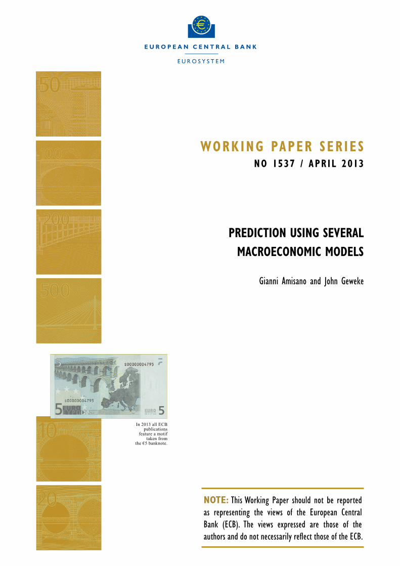
Figure 3: Each panel has one point for each of 184 quarters. The dotted line shows theleast squares �t.

The full Bayes predictive distributions and posterior mode predictive distributionshave no systematic di¤erences in location, but the former are systematically moredispersed than the latter. The intrinsic component of the predictive distribution is

22

Gaussian. The extrinsic component is not, but appears to have broadly similar decaywith increasing distance from the mode. The arithmetic of the Gaussian distributionthen implies that as realizations yt are farther from the center of the predictive distribu-tion, the corresponding log score under the posterior mode predictive distribution decaysmore swiftly than it does under the full Bayes predictive distribution.Figure 3 illustrates this e¤ect in the four models. It is exhibited most sharply in the

DSGE model and least sharply in the DFM model, but is clearly present in all four.Consistent with the evidence in Tables 3 and 4, the trade-o¤ is strongest for the VARmodels and weakest for the DSGE model. Of course, other e¤ects can be at work as well:for instance, recent behavior (yt�s, s small) that is historically atypical should magnifythe e¤ect of extrinsic uncertainty. However there is little evidence that such e¤ectsare of any quantitative importance. The main feature working to the disadvantage ofpredictive distributions based on posterior modes is their inability to account for regularbut more extreme realizations of Yt relative to full Bayes predictive distributions.

4.2 VAR models

To this point we have systematically considered two variants of VAR models, VARLand VARD. There are important di¤erences in these models, chie�y with respect tolong-run dynamics: VARL permits stationarity, random walk (with drift) and explosivebehavior, whereas VARD imposes a unit root (with drift) thus precluding stationaritybut permitting explosive behavior. These di¤erences account for the greater number ofparameters in the VARL variants. One might conjecture that the greater importanceof extrinsic variance in the VARL predictive distributions originates in the variabilityin long-run dynamics. This is reinforced by the logical implausibility of both stationaryand explosive behavior, though it seems unlikely that this would matter much in one-quarter-ahead predictive distributions.Because of the potential simplicity a¤orded in going forward with three models rather

than four in the model combination work in Section 5, we compare the VARL and VARDvariants using the log predictive scoring criterion. Table 5 compares VARL and VARDin the same way that Table 3 compared FB and PM variants of the models.For the entire period VARD performs substantially better than VARL. A formal

Bayes factor would place the odds in favor of VARD over VARL at over 1010 : 1,but this conclusion assumes that one or the other of the two models coincides withthe data generating process. The static optimal pool for the entire period stronglycontradicts this assumption, achieving an improvement of almost 20 points over VARD.This appears to be driven mainly by the pre moderation and great moderation periods.Comparisons based on PM are less interesting due to their inferiority relative to FB, butthe implications for comparison of VARD and VARL are similar.Going forward we exclude VARL from further analysis, and in particular undertake

the model combination work in Section 5 using the three models DFM, DSGE andVARD. We have also undertaken these exercises using all four models. Model poolsachieve higher log scores, but the improvements are slight compared with the dramatic

23

Table 5: Comparison of VARL and VARD predictive distributionsLog scores Pool weights Pool

Period Method VARL VARD VARL-VARD VARL VARD Log scoreEntire FB -1146.87 -1122.43 -24.45 0.380 0.620 -1102.74Entire PM -1306.41 -1265.46 -40.95 0.379 0.621 -1229.98

Pre moderation FB -599.67 -609.05 9.39 0.596 0.404 -584.60Pre moderation PM -753.80 -752.78 -1.02 0.497 0.503 -717.17Great moderation FB -430.71 -410.87 -19.84 0.124 0.876 -409.77Great moderation PM -424.40 -402.98 -21.42 0.216 0.784 -399.34Post moderation FB -116.49 -102.50 -13.99 0.000 1.000 -102.50Post moderation PM -128.21 -109.69 -18.52 0.000 1.000 -109.69

improvement in the three-model pools over any of the individual models. If VARLsubstitutes for VARD in these exercises, then the three-model pools have modestlypoorer performance. These results are consistent with the view that the predictivedistributions of the VARL and VARD models are much closer to each other than theyare to the predictive distributions of any of the other models.

4.3 Model performance

PIT tests of speci�cation clearly indicate that each model is misspeci�ed. The vari-ant of the portmanteau test (Section 3.4 and Geweke and Amisano (2012c)) in thiswork uses the �rst four moments (q = 1; 2; 3; 4) and the �rst four lagged cross-products(` = 1; 2; 3; 4) of the normalized PIT zjt (t = 1; : : : ; 184) for each constituent j = 1; : : : ; 7.For each constituent the asymptotic distribution of the moment and autocorrelation teststatistics are each �2 (4), and the asymptotic distribution of the joint test statistic is�2 (8).Table 6 reports the results of these tests using FB predictive distributions of the

models indicated in the second column for each of the seven time series indicated inthe �rst column. The p-values are based on the simulation sample of size 105 describedin Section 3.4. For reported values above 0.02 these values are close to those of theasymptotic distributions; for smaller values they are generally larger.Overall the tests indicate strong evidence against correct model speci�cation. Varia-

tion in the results is driven more by variation across constituent series than be variationacross models, with the Fed funds rate being by far the most problematic. Among theother series, the right column indicates that the strongest evidence against correct spec-i�cation arises for consumption growth, the weakest for the income growth and hoursworked index.The evidence against correct speci�cation arises more strongly in the failure to cal-

ibrate probabilities correctly on average (the moments test) than in any tendency forrealizations to persist on one side of the conditional distribution rather than the other

24

Table 6: Portmanteu probability integral transform testsMoments Autocorrelation Joint

Series Model Test p-value Test p-value Test p-valueConsumption growth DFM 104.50 0.0000 3.88 0.4077 108.37 0.0001

DSGE 32.00 0.0018 17.27 0.0040 49.28 0.0007VARD 54.24 0.0003 0.72 0.9441 54.96 0.0005

Investment growth DFM 39.19 0.0009 12.68 0.0188 51.87 0.0005DSGE 10.90 0.0325 11.43 0.0289 22.34 0.0155VARD 11.44 0.0285 10.09 0.0459 21.53 0.0178

Income growth DFM 17.03 0.0104 5.46 0.2358 22.49 0.0151DSGE 21.49 0.0057 2.74 0.5837 24.23 0.0113VARD 14.81 0.0144 4.96 0.2830 19.77 0.0355

Hours worked index DFM 5.58 0.1566 9.37 0.0591 14.96 0.0651DSGE 14.33 0.0157 14.40 0.0107 28.73 0.0060VARD 3.82 0.3111 4.47 0.3340 8.29 0.3225

In�ation DFM 18.89 0.0080 5.17 0.2629 24.06 0.0116DSGE 34.45 0.0014 55.61 0.0000 90.06 0.0001VARD 12.95 0.0205 6.53 0.1630 19.48 0.0257

Wage growth DFM 29.08 0.0026 4.62 0.3177 33.70 0.0033DSGE 24.93 0.0039 0.75 0.9397 25.68 0.0092VARD 21.92 0.0054 5.50 0.2342 27.41 0.0070

Fed funds rate DFM 937.17 0.0000 41.51 0.0000 978.69 0.0000DSGE 1619.18 0.0000 37.54 0.0000 1656.72 0.0000VARD 4130.84 0.0000 47.76 0.0000 4178.60 0.0000

25

(the autocorrelation test). Variations on these tests that use di¤erent combinations ofmoments (not reported in the table) reveal that the high values of the moments teststatistics are driven by higher order moments (especially q = 4) than by lower ordermoments (e.g. q = 1). This indicates that the di¢ culty resides in failure of subjectivepredictive distributions to be well-calibrated for outlying realizations, which occur morefrequently than these distributions imply, rather than in any failure of these distributionsto be systematically shifted relative to actual behavior.In contrast autocorrelation in realizations relative to subjective probability distribu-

tions is substantially closer to the PIT paradigm, the Fed funds rate excluded. Indeed,there is little evidence to suggest serial correlation in the probability integral transformsfor the DFM and VARD models. The evidence is somewhat stronger for DSGE but thisis mild relative to the moments test.

Figure 4: Centered 99% predictive credible intervals (top and bottom lines) and actualseries values (middle lines). Actual values outside the intervals have circles.

Figure 4 illustrates some aspects of the behavior of predictive distributions relative torealizations. In each case the upper and lower bands indicate the centered 99% intervalfor the series in question from the predictive density p (Yjt j y1:t�1; Ai). The line in thecenter indicates the corresponding realized values yjt. Whenever the realized values areoutside the 99% predictive interval the violation is indicated by a circle.For the consumption growth series (top row of panels) the models all poorly anticipate

the sharp drops in the two main recessions of the pre moderation period and in the

26

global �nancial crisis in the post moderation period. Credible intervals for the DFM aresomewhat shorter than those for the DSGE and VARD models, leading to larger thirdand fourth sample moments for z1t in the DFM. This produces the relatively high valueof the moment test statistic in the �rst line of Table 6.For the in�ation series (middle row of panels) all three models are better calibrated.

In the case of the DFM and VARD models all realizations are within the 99% credibleinterval. During the pre moderation period actual in�ation tends to be persistently tothe right side of the predictive distribution. This is especially evident in the DSGEmodel, which for this series has the largest of all the autocorrelation test statistics inTable 6.The last row of panels of Figure 4 indicates that the extremely poor calibration of

the models for the Fed funds rate conveyed by the last three rows of Table 6 originatesin the pre moderation period. The models poorly anticipate the many large upwardand downward movements in this period. This is not surprising, given the much moremoderate behavior of interest rates prior to 1970 (Table 1), which drives the posteriordistribution going into this period. The posterior distributions adjust to this morevolatile behavior: note how much wider the predictive intervals are during and after thegreat moderation than they are in the late 1960�s and early 1970�s. For the Fed fundsrate predictive intervals for the VARD remain somewhat narrower than those for theDFM and DSGE models in the 1970 - 1983 period, leading to larger PIT test statisticsin Table 6.The condition that one of the models includes the data generating process as a special

case underlies formal Bayesian inference from multiple models, and is central to manynon-Bayesian procedures as well. Any credibility that this condition might have hadis refuted by the PIT tests. This suggests that procedures for prediction using severalmodels that do not invoke this condition might produce superior predictions.

5 Model combination

Given several alternative models constructed for the purpose of assigning probabilitiesto future events, it is natural to investigate whether it is possible to combine models toaccomplish this goal more e¤ectively than would be possible with any one model alone.The linear pool (5) has been the dominant approach in the literature in combiningpredictive densities. Wallis (2011) reviews these approaches, including the log pools ofGenest and Zidek (1986). When future events are functions of several random variables,as is the case here with Yt, we �nd the result of McConway (1981) compelling: that papershows that, under mild regularity conditions, the combination must be of the form (5)if the process of combination is to commute with any possible marginalization of thedistributions involved. After summarizing the behavior of some selected static pools(Section 5.1) we turn to three kinds of linear pools: those with equal weights (Section5.2), pools arising from Bayesian model averaging (Section 5.3), and real time optimalpools (Section 5.4). All of the analysis in this section is based on full Bayesian predictive

27

distributions of the DFM, DSGE and VARD models.

5.1 Pools

Let f (wr:t) denote the summation on the right side of (7). This function conveys theperformance of any possible linear pool with constant weights over the period from r tot, using the log scoring rule to assess performance. Figure 5 depicts the function for thefour periods of interest. The domain is the three-dimensional unit simplex, depicted intwo dimensions in the usual way. In all four panels the horizontal axis corresponds tothe weight on the DFM model and the vertical axis to the weight on the DSGE model.Thus the value of f (wr:t) at the right vertex corresponds to the log score of the DFMmodel over the indicated period, at the upper vertex to the DSGE model, and at theorigin to the VARD model. These values are indicated in Table 7.The contours in each panel indicate [argmaxwrt f (wr:t)]�f (wr:t), and are chosen to

show increments of 0:025 (t� r + 1), corresponding to increments of 0.025 in the arith-metic mean of log [

Pni=1wip(ys j ys�1; Ai] over the period in question. An increase from

one contour to the next corresponds to an increase in the proportion exp (0:025) � 1,or about 2.5%, in the geometric mean of the probability density assigned to observedevents. This makes the contours directly comparable across periods of unequal length.Notice that the log score f (wr:t) is much less sensitive to changes in wr:t near its maxi-mum, indicated by the asterisk in each panel of Figure 5, than it is to changes close tothe vertices of the simplex.

5.2 Equally weighted pools

An equally weighted pool, wi = 1=3 (i = 1; 2; 3), is arguably the simplest pool that couldbe created. These pools are indicated by the � in each panel of Figure 5. It is evidentthat such pools improve markedly on the log score of any given model. The log scoreof the equally weighted pool is also close to the maximum log score indicated by theasterisk. But this maximum log score is unattainable in real time, because the weightvector achieving this maximum is chosen on the basis of all the data for the period inquestion. This suggests that an equally weighted pool is likely to be a strong competitorfor prediction using all three models. Subsequent analysis in this section veri�es thisconjecture.Table 7 quanti�es the gains from pooling with equal weights that is evident in Figure

5. The second column is the log score of the equally weighted pool, indicated by the� in each panel of Figure 5. The entries in columns 3 through 5 are the log scores ofthe FB variants of the indicated models (see Table 3) minus the EWP log scores. Eachof the last three columns measures the value of the corresponding model in an equallyweighted pool as the di¤erence between the log score of the equally weighted pool withall three models and an equally weighted pool composed of the other two models. Forexample, the entry 32.10 for DFM for the whole period is the di¤erence between the logscore of the equally weighted pool (X in the upper left panel of Figure 5), and the log

28

Figure 5: Log scores of pools as a function of the weight vector wr:t in (7), normalizedso that the maximum value is the same. Distance between contours is 0:025 (t� r + 1).

score of the equally weighted pool of the DSGE and VARD models (the square on thevertical axis in this panel). Clearly value measured in this way need not be positive, butit generally is. The DFM has the greatest value in every period except post moderation.The equally weighted pool also provides a useful benchmark in understanding the

gains from pooling and the reason that the DFM is the most valuable contributor to thepool. The left panels of Figure 6 show the model log predictive scores in all 184 quarters.These log scores tend to move together: the correlation coe¢ cient is over 0.9 for all pairsand is driven in large part by extreme events that are assigned low predictive probabilityby all three models. The right panels of the �gure show the di¤erences between modellog scores and the log score of the equally weighted pool. This di¤erence cannot exceedlog (3), which is the highest value on the vertical axis in these panels. There is no lowerbound.The vertical lines in Figure 6 denote the twelve quarters in which the mean predictive

log score, taken over the three models, was the lowest. In these quarters di¤erences inmodel log scores also tend to be greatest, because these three models di¤er substantiallyin the probabilities they assign to rare events. This can be detected in the left column ofpanels but is more evident in the right column where the equally weighted pool is usedas a common benchmark. In many of these quarters, one of the models substantiallyoutperforms the other two, leading to a log score relative to the equally weighted pool

29

Table 7: Log scores of models (with full Bayesian inference) and the equally weightedpool

Log score Relative to EWP Model valuesPeriod EWP DFM DSGE VARD DFM DSGE VARD

Entire -1036.72 -47.13 -60.31 -85.70 32.10 12.08 12.58Pre moderation -526.06 -14.59 -33.68 -82.99 27.68 10.44 -0.67Great moderation -411.36 -26.61 -25.19 0.49 4.31 -1.45 12.93Post moderation -99.30 -5.93 -1.45 -3.20 0.11 3.09 0.32

that is close to log 3 for that model, but low values for the other two models. The DFMenjoys this distinction most often. The only notable exception is the �nal quarter of2008, where the DSGE outperformed the DFM and VARD.The DFM contributes the pool in a manner similar to a �nancial asset that moves

against the market. For the di¤erences shown in the right column of panels in Figure 6,the DFM is negatively correlated with both the DSGE (-0.501) and the VARD (-0.313),whereas the DSGE and VARD are positively correlated (0.268). This property of theDFM, together with its higher log score, accounts for the fact that the DFM has thehighest value in the equally weighted pool (Table 7).This analysis tends to obscure the asymmetric behavior of the three models with

respect to outlying events that is evident in Figure 6. Figure 7 highlights the di¤erentproperties of the models in this dimension. It cumulates di¤erences between the logpredictive scores of the models and the log predictive score of the equally weighted pool,over quarters ordered by the mean of the log predictive score over models, lowest tohighest. Thus the twelve quarters highlighted in Figure 6 correspond to the values 1through 12 on the horizontal axis. For quarter 184 the values are those in the �rst rowof entries in Table 6, columns 3 through 5. Through the 50 quarters with the lowestpredictive log scores, the DFM dominates: its log score is very nearly that of the equallyweighted pool. These same quarters account all of the de�ciency in the predictive logscore of the VARD; indeed it more than accounts for this di¤erence, because the valueof the VARD performs best, relative to the EWP, in those quarters in which model logscores are highest. This is also consistent with the strong performance of the VARDrelative to the other two models during the great moderation (Figure 5).The improvement in predictive log score achieved in moving from any one model to

the equally weighted pool is comparable to the gain in moving from posterior mode tofull Bayes predictive densities in each model. For the DFM, DSGE and VARD modelsthe average gain from the former was 64.39 (minus the average of relative log scores forthe entire period in Table 7) and the average gain from the latter was 75.15 (�fth columnof Table 3 for the entire period). Analysis of predictive variance for the pool with equalweights (11) leads to the same conclusion, as indicated in Table 8.This table reports two di¤erent approximations of the decomposition. The �rst

one (columns 2 through 4) uses the expressionPn

i=1wi��it�1 � �t�1

� ��it�1 � �t�1

�0to

30

Figure 6: Model predictive log scores by quarter, absolutely (left panels) and relativeto the equally weighted pool (right panels). Vertical lines indicate the 12 quarters forwhich the mean values taken over the model predictive log scores are the smallest.

approximate varAi [E (Yt+1 j Ai)] just as described in Section 3.3, using the equal weightswi = 1=3 (i = 1; 2; 3). This preserves the identity (11) when the estimates are substitutedfor the population values. But this also leads to the usual downward bias in the varianceestimate, which is severe here because there are only three di¤erent models. Columns5 through 7 use wi = 1=2 (i = 1; 2; 3), which alleviates the bias. The �within�extrinsicvariance is that which drove the better performance of FB log scores relative to PM logscores, as argued in Section 4.1; the �between�extrinsic variance is due to di¤erencesbetween models, which drives the improvement in the log predictive scores of the equallyweighted pool relative to the individual models. The order of magnitude is similar,supporting the �nding that pooling and the use of full Bayes predictive distributions areof comparable importance in improving predictions using several models.

5.3 Bayesian model averaging

As discussed in Section 3.1, di¤erences between models in log scores for full Bayesprediction are closely related to Bayes factors and posterior odds ratios. Precisely,

LSr:t (Ai) =tXs=r

log p (ys j y1:s�1; Ai)

31

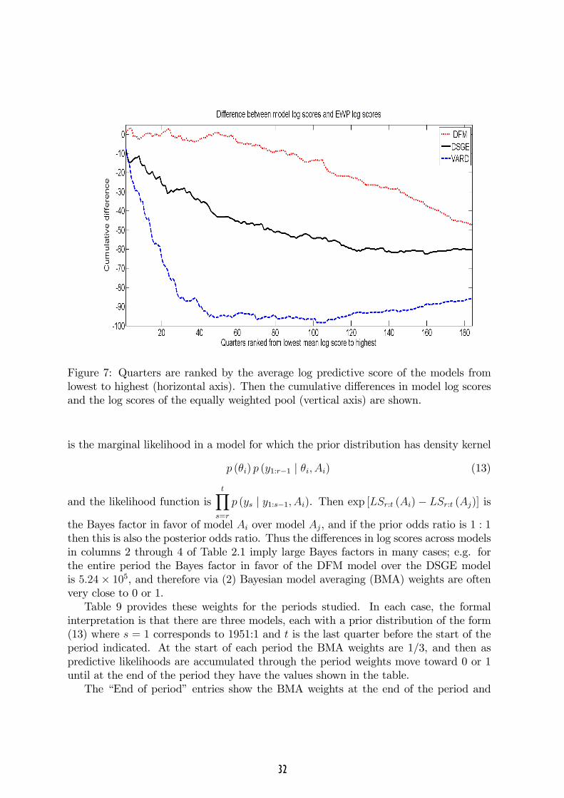
Figure 7: Quarters are ranked by the average log predictive score of the models fromlowest to highest (horizontal axis). Then the cumulative di¤erences in model log scoresand the log scores of the equally weighted pool (vertical axis) are shown.

is the marginal likelihood in a model for which the prior distribution has density kernel

p (�i) p (y1:r�1 j �i; Ai) (13)

and the likelihood function istYs=r

p (ys j y1:s�1; Ai). Then exp [LSr:t (Ai)� LSr:t (Aj)] is

the Bayes factor in favor of model Ai over model Aj, and if the prior odds ratio is 1 : 1then this is also the posterior odds ratio. Thus the di¤erences in log scores across modelsin columns 2 through 4 of Table 2.1 imply large Bayes factors in many cases; e.g. forthe entire period the Bayes factor in favor of the DFM model over the DSGE modelis 5:24� 105, and therefore via (2) Bayesian model averaging (BMA) weights are oftenvery close to 0 or 1.Table 9 provides these weights for the periods studied. In each case, the formal

interpretation is that there are three models, each with a prior distribution of the form(13) where s = 1 corresponds to 1951:1 and t is the last quarter before the start of theperiod indicated. At the start of each period the BMA weights are 1/3, and then aspredictive likelihoods are accumulated through the period weights move toward 0 or 1until at the end of the period they have the values shown in the table.The �End of period� entries show the BMA weights at the end of the period and

32

Table 8: Decomposition of extrinsic variance in the equally weighted poolFraction of variance extrinsic

Adding-up preserved Unbiasedness preservedSeries Within Between Total Within Between TotalConsumption growth 0.0507 0.0690 0.1197 0.0491 0.0982 0.1473Investment growth 0.0523 0.0494 0.1017 0.0508 0.0707 0.1216Income growth 0.0496 0.0460 0.0956 0.0483 0.0662 0.1145Hours worked index 0.0489 0.0385 0.0874 0.0477 0.0551 0.1027In�ation 0.0583 0.0645 0.1228 0.0563 0.0913 0.1476Wage growth 0.0598 0.0419 0.1017 0.0585 0.0606 0.1191Fed funds rate 0.0469 0.0695 0.1164 0.0448 0.0950 0.1398

Table 9: Bayesian model averaging weights and log scoresEnd of period Average over period

Model BMA weights Log Model BMA weights LogPeriod DFM DSGE VARD score DFM DSGE VARD score

Entire 1.0000 0.0000 0.0000 -1083.86 0.9111 0.0656 0.0234 -1084.96Pre moderation 1.0000 0.0000 0.0000 -540.66 0.7849 0.1585 0.0566 -541.75

Great moderation 0.0000 0.0000 1.0000 -410.87 0.0055 0.0406 0.9540 -411.97Post moderation 0.0095 0.8446 0.1459 -99.93 0.0910 0.7472 0.1618 -101.68

the log score that results when these weights are applied to the model log scores for theentire period. This is the log score for BMA most commonly reported, but it cannotbe achieved in real time. The �Average over period�entries are based on BMA weightsupdated each observation in the period, with average weights shown. The log score is�gured by applying the BMA weights updated through period t � 1 to the predictivedensities for period t, which are then evaluated at yt.The DFM strongly dominates the entire period and pre moderation; VARD strongly

dominates the great moderation; and DSGE weakly dominates the post moderation. InFigure 5 the BMA weights are indicated by the triangle in each panel, and the �fthcolumn of Table 9 shows the corresponding log predictive scores for the Bayesian modelaverages. They are all lower than the log scores of the equally weighted poolSuppose a Bayesian econometrician maintained the hypothesis underlying BMA: that

the data generating process is exactly p (Yt j Y1:t�1; ��i ; Ai) for some one of the models Aiand some particular value ��i of that model�s parameter vector, though which model andwhich speci�c values of the parameter vector are unknown. Were this econometricianto have started to work at the end of 1965, using (13) as the kernel of her prior density,then her BMA weights would have evolved as indicated in the upper panel of Figure8.3 The sum of the BMA weights on the DFM and DSGE models drops below 0.1 in

3This exercise is consistent with the values in Table 9 for the entire period and the pre moderation

33

Figure 8: Bayesian model averaging and optimal pool weights updated each quarter

the last quarter of 1971, and below 0.01 the following quarter where it remains for therest of the entire period. The largest sum of BMA weights on the DFM and DSGEmodels in the rest of the entire period is 0.00345 in the �rst quarter of 1998, and formost quarters beyond 1972:1 the sum is less than 10�6. This is all consistent with thetypical asymptotic distribution of BMA weights outlined in Section 3.1.

5.4 Optimal pooling

Optimal pools can be constructed for any period as described in Section 3.2, leadingto the weight vector w�

r:t (7), and the corresponding log score for the optimal pool isthen given by the summation on the right side of (7) evaluated at the optimal weights.These weights, and related statistics, provide useful summaries of the interaction betweenmodels in prediction over particular time periods. However, they could not have beenused in real time during the period in question, and any pooling procedure that could beused would lead to a lower log score for the resulting pool. The optimal weights couldbe used going forward, for example in quarter t+ 1.In each panel of Figure 5 the asterisk indicates the weights for the optimal pool

formed this way, and columns 2 through 4 of Table 10 provide their values. The value

period, because these exercises all start in 1966:1. It is not consistent with the values in Table 9 forthe great moderation and post moderation periods because those calculations begin at the start of therespective periods.

34

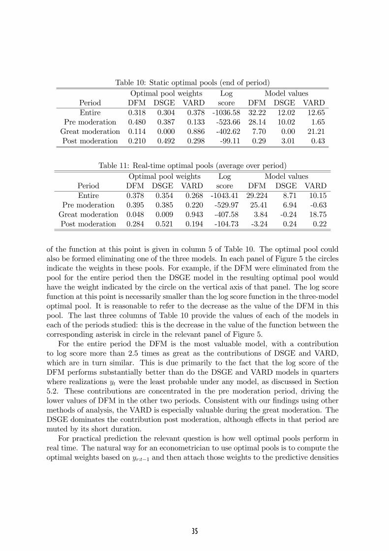
Table 10: Static optimal pools (end of period)Optimal pool weights Log Model values

Period DFM DSGE VARD score DFM DSGE VARDEntire 0.318 0.304 0.378 -1036.58 32.22 12.02 12.65

Pre moderation 0.480 0.387 0.133 -523.66 28.14 10.02 1.65Great moderation 0.114 0.000 0.886 -402.62 7.70 0.00 21.21Post moderation 0.210 0.492 0.298 -99.11 0.29 3.01 0.43

Table 11: Real-time optimal pools (average over period)Optimal pool weights Log Model values

Period DFM DSGE VARD score DFM DSGE VARDEntire 0.378 0.354 0.268 -1043.41 29.224 8.71 10.15

Pre moderation 0.395 0.385 0.220 -529.97 25.41 6.94 -0.63Great moderation 0.048 0.009 0.943 -407.58 3.84 -0.24 18.75Post moderation 0.284 0.521 0.194 -104.73 -3.24 0.24 0.22

of the function at this point is given in column 5 of Table 10. The optimal pool couldalso be formed eliminating one of the three models. In each panel of Figure 5 the circlesindicate the weights in these pools. For example, if the DFM were eliminated from thepool for the entire period then the DSGE model in the resulting optimal pool wouldhave the weight indicated by the circle on the vertical axis of that panel. The log scorefunction at this point is necessarily smaller than the log score function in the three-modeloptimal pool. It is reasonable to refer to the decrease as the value of the DFM in thispool. The last three columns of Table 10 provide the values of each of the models ineach of the periods studied: this is the decrease in the value of the function between thecorresponding asterisk in circle in the relevant panel of Figure 5.For the entire period the DFM is the most valuable model, with a contribution

to log score more than 2.5 times as great as the contributions of DSGE and VARD,which are in turn similar. This is due primarily to the fact that the log score of theDFM performs substantially better than do the DSGE and VARD models in quarterswhere realizations yt were the least probable under any model, as discussed in Section5.2. These contributions are concentrated in the pre moderation period, driving thelower values of DFM in the other two periods. Consistent with our �ndings using othermethods of analysis, the VARD is especially valuable during the great moderation. TheDSGE dominates the contribution post moderation, although e¤ects in that period aremuted by its short duration.For practical prediction the relevant question is how well optimal pools perform in

real time. The natural way for an econometrician to use optimal pools is to compute theoptimal weights based on yr:t�1 and then attach those weights to the predictive densities

35

p (Yt j y1:t�1; Ai). Speci�cally, the econometrician �nds

w�r:t�1 = argmax

w

t�1Xs=r

log

"nXi=1

wip (ys j yr:s; Ai)#

and then uses the predictive densitynXi=1

w�r:t�1;ip (Yt j yr:t�1; Ai)

for quarter t.Table 11 reports some aspects of the results of this procedure. For period indicated

in the table, r is the �rst quarter in the period. For each period the average weightsin columns 2 through 4 are the elements of (u� r + 1)�1

Put=rw

�rt, where u is the last

quarter in the period. The log score in column 5 is the predictive likelihood for thisreal-time optimal pool,

uXt=r

log

"nXi=1

w�r;t�1;ip (yt j yr:t�1; Ai)#, (14)

with w�r;r�1;i = n�1. Thus the log scores in this column are directly comparable withthose for individual models, equally weighted pools, and Bayesian model averaging: allreport results an econometrician could have achieved in real time.Log scores of real-time optimal pools are, algorithmically, lower than those of static

optimal pools for the same period. Comparisons of the corresponding entries of Tables10 and 11 show that the decrease is between 5 and 7 points in each period. Moresigni�cantly, the equally weighted pool (Table 9) outperforms the real-time optimalpool in three of the four periods examined. Only in the great moderation, in which thethree models display the greatest asymmetry (Figure 5), does the equally weighted poolfall short of the real-time optimal pool.The last three columns of Table 11 provide real-time model values, parallel to the

values for static optimization in Table 10. For each model the real-time optimal pool-ing exercise is repeated eliminating that model but retaining the others. The value isthe di¤erence between the original log predictive likelihood (14) and the correspondingexpression with the model eliminated. Such model values are not algorithmically non-negative, as is the case in the static optimal pool. All model values for all periods arelower in the real-time optimal pool (Table 11) than in the corresponding static opti-mal pool (Table 10), and the two models with the lowest values in the latter pool havenegative values here.

6 Conclusion

The principal conclusion of this work is that predictions are best formed from severalmacroeconomic models by pooling the Bayesian predictive distributions of the models.

36

Table 12: Real-time log scores of models and pools, entire periodModel log scores Model pooling

Model PM FB FB-PM Method Log scoreDFM -1135.10 -1083.86 51.24 BMA -1084.96DSGE -1128.23 -1097.03 31.20 RTOP -1043.41VARD -1265.46 -1122.43 143.03 EWP -1036.72Mean -1176.26 -1101.11 75.15

This is supported by multiple analyses that contribute to the understanding of this�nding. We think it likely that similar �ndings would also emerge in other data sets,though the postwar US data is unique in extent, continuity and quality; and also withother families of models, either existing or yet to be formulated, of similar intellectualand empirical pedigree.The procedures used here emulate what could have been done in �real time� by

adding the most recent quarter�s data and updating posterior distributions accordinglyat the end of each quarter for the purposes of predicting the following quarter. Theresults do not attempt to use the data releases actually at hand each quarter; we doubtthat this extension would overturn the main �ndings in this work. Table 12 summarizesthe main quantitative results for the entire postwar US data set.The �rst part of the principal conclusion is that gains to using full Bayesian (FB)

predictive distributions, as opposed to a �plug in�distribution that replaces the randomparameter vector with its value at the posterior mode (PM), are substantial. In Table 12the posterior mode predictive log score, averaged across the three models, falls short ofthe average for the full Bayes predictive distributions by 75.15 points. To appreciate thisdi¤erence, it implies that the full Bayes predictive distributions increase the geometricaverage of the probabilities p (yt j y1:t�1; Ai) of the observed Yt over the period 1966 -2011 by 100 [exp (75:15=184)� 1]% = 50:4% on average over the three models.The key de�ciency with the posterior mode is its failure to account for parameter

uncertainty, and therefore extends to any �plug in�procedure. This is consistent witheconometric theory. The analysis in Section 4 linked the results to this theory froma number of analytical perspectives that shed further light on the circumstances thatmagnify the di¤erences. Parameter uncertainty is increasingly important moving fromthe DSGE, to the DFM, to the VARD model, gauged either by the crude measure ofnumber of parameters or the more precise measure of the extrinsic fraction of predictivevariance, and this accounts for the di¤erences in models in column 4 of Table 12.Thisinterpretation implies that these di¤erences will be most manifest when realizationsin the quarter predicted are at the lowest ranges of the predictive densities, and thisimplication is borne out in the analysis. In the context of a single model, the fullBayesian predictive distribution is not only formally more correct, it is essential tocompetitive prediction.The second part of the principal conclusion is that further gains, of a similar order

37

of magnitude, can be accomplished by pooling. This study examined three variantsof pooling: Bayesian model averaging (BMA), real-time optimal pooling (RTOP) andequally weighted pools (EWP), all using full Bayesian predictive distributions. Bayesianmodel averaging puts essentially the entire weight on the DFM model, consistent withthe common �nding that in large data sets the model with the highest marginal likelihooddominates the other models. The resulting BMA log score is closer to the mean of theindividual models using FB than it is to either the RTOP or EWP log scores. Boththe RTOP and the EWP improve substantially on the mean log scores of the modelsusing FB, by 57.70 and 64.39 points, respectively. This is comparable with the gainsmade in moving from PM to FB in the individual models. For the EWP the increasein the geometric average of the probabilities of the observed Yt over the period 1966-2011 is 41:9%. Combining this with the previous improvement with FB over PM, theEWP increases the geometric average of these probabilities by 113:5% relative to PMpredictive distributions in a single model.BMA conditions on one of the models actually being the data generating process,

and the log score of one model often dominates that of the others even in samples ofmodest size. Taken together, this virtually eliminates any posterior uncertainty aboutwhich model is �true.� But the condition is not credible. Di¤erent models capturedi¤erent aspects of reality. Their log scores move together, but each bears a distinctrelationship to the average log score. In these circumstances there are gains to usinga linear combination of predictive densities even when it is quite clear which is higheston average. The situation is analogous (though the math is not identical) to portfoliodiversi�cation, in which major gains accrue even when diversi�cation is not optimal.If there is in fact a true data generating process underlying reality, then given stan-

dard side conditions there is a limiting value for the weight vector in the optimal pool(Geweke and Amisano, 2011). If the econometrician knew that vector then eventuallythe pool using that vector would outperform the EWP in log score. Of course the vectoris really unknown, and the RTOP uses a weight vector that changes from quarter toquarter and thereby introduces noise, especially when there are few observations. Logscores of pools are not very sensitive to weights until some of the weights approach zero,and consequently it can be the case that �xed reasonable weights outperform an e¤ortto re-optimize the pool each quarter.

38

References

An S, Schorfheide F (2007). Bayesian analysis of DSGE models. Econometric Reviews26: 113-172.

Balke N, Gordon R J (1986). Appendix B. Historical Data. In Gordon R J (Ed.), TheAmerican business cycle: continuity and change. NBER and University of ChicagoPress.

Berkowitz J (2001). Testing density forecasts with applications to risk management.Journal of Business and Economic Statistics 19: 465-474.

Bernanke B, Boivin J (2003). Monetary policy in a data-rich environment. Journal ofMonetary Economics 50: 525-546.

Bernardo J, Smith AFM (1993). Bayesian Theory. Oxford: Oxford University Press.

Del Negro M, Schorfheide F (2004). "Priors from General Equilibrium Models forVARs", International Economic Review 45: 643-673.

Del Negro M, Schorfheide F (2012). Del Negro M.and F. Schorfheide (2012): "DSGEModel-Based Forecasting", prepared for Handbook of Economic Forecasting, Vol-ume 2.

Doan T, Litterman R, Sims CA (1984). Forecasting and conditional projection usingrealistic prior distributions. Econometric Reviews 3: 1�100.

Doucet A, Godsill S, Robert C. (2002). Marginal maximum a posteriori estimationusing Markov chain Monte Carlo. Statistics and Computing 12: 77�84.

Forni M, Hallin M, Lippi M, Reichlin L (2005). The generalized dynamic factor model.One-sided estimation and forecasting. Journal of the American Statistical Associ-ation. 100: 830�840.

Genest C, Zidek JV (1986). Combining probability distributions: a critique and anan-notated bibliography (with discussion), Statistical Science 1: 114�48.

Geweke J (1977). The dynamic factor analysis of economic time series models. In DAigner and A Goldberger (eds) Latent Variables in Socioeconomic Models 365-383Amsterdam. North-Holland.

Geweke J, Amisano G (2010). Evaluating the predictive distributions of Bayesianmodels of asset returns. International Journal of Forecasting 26: 216-230.

Geweke J, Amisano G (2011). Optimal prediction pools. Journal of Econometrics164:130-141.

39

Geweke J, Amisano G (2012a). Prediction with misspeci�ed models. American Eco-nomic Review Papers and Proceedings 102,3: 482�486.

Geweke J, Amisano G (2012b). Analysis of variance for Bayesian inference. Economet-ric Reviews, forthcoming.

Geweke J, Amisano G (2012c). Portmanteau probability integral transform tests.Working paper in preparation.

Ingram B., Whiteman C (1994). Supplanting the Minnesota Prior- Forecasting Macro-economic Time Series Using Real Business Cycle Model Priors. Journal of Mone-tary Economics 49: 1131�159.

Ireland P. (2004). A method for taking models to the data. Journal of EconomicDynamics and Control 28: 1205-1226.

Litterman R (1986). Forecasting With Bayesian vector autoregressions: �ve years ofexperience Journal of Business and Economic Statistics 4: 25�38.

McConnell M, Pérez-Quirós G (2000). Output �uctuations in the United States. Whathas changed since the early 1980s? American Economic Review. 90: 1464-1476.

McConway KJ (1981). Marginalization and linear opinion pools. Journal of the Amer-ican Statistical Association 76: 410-414.

Rosenblatt, M. (1952). Remarks on a multivariate transformation. Annals of Mathe-matical Statistics 23: 470-472.

Sargent T. (1989). Two models of measurements and the investment accelerator, Jour-nal of Political Economy 97: 251�287.

Sargent T, Sims CA (1977). Business cycle modeling without pretending to have toomuch a-priori economic theory, in: C. Sims et al., eds., New methods in businesscycle research (Federal Reserve Bank of Minneapolis, Minneapolis).

Sims, CA (1980). Macroeconomics and reality. Econometrica 48: 1-48.

Smets F, Wouters R (2003). An estimated dynamic stochastic general equilibriummodel of the euro area. Journal of the European Economic Association. 1: 1123�1175.

Smets F, Wouters R (2007). Shocks and frictions in US business cycles: A BayesianDSGE approach. American Economic Review 97: 586-606.

Smith JQ (1985). Diagnostic checks of non-standard time series models. Journal ofForecasting 4: 283-291.

40

Stock JH, Watson MW (2002a). Forecasting using principal components from a largenumber of predictors. Journal of the American Statistical Association. 97: 147-162.

Stock JH, Watson MW (2002b). Has the business cycle changed and why? NBERMacroeconomics Annual 2002, Mark Gertler and Ken Rogo¤ (eds), MIT Press.

Stock JH, Watson MW (2005). Implications of Dynamic Factor models for VAR analy-sis. NBER Working Paper 11467.

Waggoner DF, Zha T (2012). Confronting model misspecication in macroeconomics.Journal of Econometrics, forthcoming.

Wallis KF (2011). Combining forecasts - forty years later. Applied Financial Economics21: 33-41.

41