Predictiv e Model for Human-Unmanned Vehicle Sy stems

Predictive Model for Human-Unmanned Vehicle Systems

The MIT Faculty has made this article openly available. Please share how this access benefits you. Your story matters.

Citation Crandall, Jacob W., M. L. Cummings, and Carl E. Nehme. “PredictiveModel for Human-Unmanned Vehicle Systems.” Journal ofAerospace Computing, Information, and Communication 6, no. 11(November 2009): 585-603.

As Published http://dx.doi.org/10.2514/1.39191

Publisher American Institute of Aeronautics and Astronautics

Version Author's final manuscript

Citable link http://hdl.handle.net/1721.1/81769

Terms of Use Creative Commons Attribution-Noncommercial-Share Alike 3.0

Detailed Terms http://creativecommons.org/licenses/by-nc-sa/3.0/

https://libraries.mit.edu/forms/dspace-oa-articles.html

http://hdl.handle.net/1721.1/81769

http://creativecommons.org/licenses/by-nc-sa/3.0/

A Predictive Model for Human-Unmanned Vehicle

Systems

Jacob W. Crandall ∗

Masdar Institute of Science and Technology, Abu Dhabi, UAE

M. L. Cummings,†

Massachusetts Institute of Technology, Cambridge MA 02139

Carl E. Nehme ‡

McKinsey & Company, Dubai, UAE

Advances in automation are making it possible for a single operator to control multipleunmanned vehicles (UVs). However, the complex nature of these teams presents a difficultand exciting challenge for designers of human-UV systems. To build such systems effec-tively, models must be developed that describe the behavior of the human-UV team andthat predict how alterations in team composition and system design will affect the system’soverall performance. In this paper, we present a method for modeling human-UV systemsconsisting of a single operator and multiple independent UVs. Via a case study, we demon-strate that the resulting models provide an accurate description of observed human-UVsystems. Additionally, we demonstrate that the models can be used to predict how changesin the human-UV interface and the UVs’ autonomy alter the system’s performance.

I. Introduction

Many important missions, including search and rescue, border security, and military operations, requirehuman reasoning to be combined with automated unmanned vehicle (UV) capabilities to form a synergis-tic human-UV system. However, the design and implementation of such systems remains a difficult andchallenging task. Challenges related to the operators, the UVs, and the interactions between them must beaddressed before human-UV systems will realize their full potentials.

To understand and address these issues more fully, comprehensive models of human-UV systems shouldbe developed. These models should have two important capabilities. First, they should adequately describethe behavior and performance of the team and the system as a whole. Second, these models should be ableto accurately predict the behavior and performance of the team as the environment, mission, or human-UVsystem changes.

Models with both descriptive and predictive abilities have a number of important uses. For example, suchmodels can improve the design processes of human-UV systems. As in any systems engineering process, testand evaluation plays a critical role in fielding new technologies. In systems with significant human-automationinteraction, testing with representative users is expensive and time consuming. Thus, the development of ahigh-fidelity model of a human-UV system with both descriptive and predictive capabilities could streamlinethe test and evaluation cycle by diagnosing causes of previous system failures and inefficiencies, and indicatinghow potential design modifications will affect the behavior and performance of the system.

A model with both descriptive and predictive capabilities can also be used to determine successful teamcompositions. The composition of human-UV teams can potentially change dynamically both in number and∗Assistant Professor, Information Technology Program, Abu Dhabi, UAE†Associate Professor, Department of Aeronautics and Astronautics, Cambridge MA 02139. AIAA Associate Fellow‡Associate, McKinsey & Company, Dubai, UAE

1 of 18

American Institute of Aeronautics and Astronautics

type of UVs due to changing mission assignments and resource availability. High-fidelity models can be usedto ensure that changes in team composition will not cause system performance to drop below acceptablelevels. Furthermore, given the team composition, these models can suggest which autonomy levels the UVsshould employ.

As a step toward developing such high-fidelity and comprehensive models, we propose a method formodeling human-UV systems. Due to the need to reduce manning in current human-UV systems,1 we focuson modeling human-UV systems consisting of a single operator and multiple homogeneous and independentUVs. The modeling method can be used to model systems employing any level of automation.2–5 However,we assume that the operator interacts with each UV in the team individually, rather than in a group.6

The remainder of this paper proceeds as follows. In Section II, we define a stochastic model of human-UV systems consisting of a single operator and multiple independent UVs. Section III describes how thisstochastic model is constructed using observational data. In Section IV, we describe a user study in whichusers controlled simulated UVs to perform a search and rescue mission. Observational data from this studyis used to model the human-UV team and predict how changes in the system would alter its performance.In Section V, these predictions are compared with observed results. We conclude and discuss future work inSection VI.

II. Modeling Human-UV Systems

The behavior of a human-UV system consisting of a single operator and multiple independent UVscan be described with a set of models.7 Each model describes the behavior of a particular aspect of thesupervisory control system given a characterization of the system’s state. In this paper, we use separatemodels to describe the behaviors of the operator and the individual UVs in the system. When combined,these individual models form a description of the behavior of the entire human-UV system. In this section,we describe the separate models and how they are combined. We begin by defining useful notation andterminology.

II.A. Notation and Terminology

The models described in this paper are characterized by the notion of system state, which we define with thetuple σ = (s, τ). The first element, s, characterizes the state of each of the individual UVs in the team. LetS be the set of possible UV states, and let si ∈ S be the state of UV i. Then, s = (s1, · · · , sN ) is the jointstate of a team of N UVs. The second element of system state σ is mission time τ . Mission time, whichis important to consider when modeling time-critical operations, refers to the time elapsed since the teambegan performing its current mission. We denote Σ as the set of possible system states.

II.B. Modeling UV Behavior

In previous work, the performance of a UV is modeled with respect to the temporal metrics of neglect timeand interaction time.8–10 Neglect time is the expected amount of time that a UV maintains acceptableperformance levels in the absence of interactions (with the operator). Interaction time is the average amountof time an operator must interact with a UV to restore or maintain desirable UV performance levels. Pairedtogether, these metrics identify the automated capability of a UV as well as the average frequency andduration of interactions necessary to keep the UV’s performance above some threshold.10 In particular,neglect time and interaction time can be used to estimate the amount of time an operator must devote to asingle UV11 and the maximum number of UVs that a single operator can effectively control (Fan-out).9

While neglect time and interaction time are valuable and informative metrics, they are not rich enoughto sufficiently describe and predict many relevant aspects of UV behavior.7 One potential alternative is tomodel UV behavior with two sets of random processes,7,10 which we call interaction impact (II) and neglectimpact (NI), respectively. These random processes describe a UV’s behavior or performance in the presenceand absence of interactions, respectively.

In this paper, we model UV behavior with state transitions. Thus, the random processes II and NIdescribe how a UV’s state changes over time. Formally, let σ ∈ Σ be the system state when the operatorbegins interacting with UV i. The random process II(σ) stochastically models how UV i’s behavior changesits state si throughout the duration of the interaction. The time variable of the process takes on all valuesin the interval [0, L], where L is the length of the interaction and t = 0 corresponds to the time that

2 of 18


the interaction began. Thus, for each t ∈ [0, L], II(σ; t) is a random variable that specifies a probabilitydistribution over UV states.

Likewise, we model the behavior of a UV in the absence of human attention with a random process. Letσ ∈ Σ be the system’s state at the end of the UV’s last interaction. Then, the random process NI(σ)describes the UV’s state transitions over time in the absence of additional interactions. Hence, for eacht ∈ [0,∞), where t = 0 corresponds to the time that the UV’s last interaction ended, NI(σ; t) is a randomvariable that specifies a probability distribution over UV states.

We note that the structures II(σ) and NI(σ) assume that UV behavior is Markovian with respect tothe system state σ at the beginning and end of the interaction, respectively. In large part, the accuracyof the Markov assumption is dependent on the set of UV states (S). We note also that when the UVsperform independent tasks, the behavior of each individual UV in the presence and absence of interactionsis independent of the states of the other UVs in the team. Since we assume independence in this paper,II(σ) = II(si, τ) and NI(σ) = NI(si, τ).

II.C. Modeling Operator Behavior

The operator plays a crucial role in the success of a human-UV system. Thus, a high-fidelity model of ahuman-UV system must account for the behavior of the operator. Since II(σ) and NI(σ) are driven byhuman input, they implicitly model human behavior during interactions. However, these structures do notaccount for how the operator allocates attention to the various UVs in the team. Previous work has identifiedtwo important aspects of operator attention allocation: selection strategy and switching time. The operator’sselection strategy refers to how the operator prioritizes multiple tasks.12–14 Switching time is the amount oftime the operator spends determining which UV to service.15,16

As with UV behavior, temporal metrics can be used to measure operator attention allocation. Onesuch set of metrics involves the concept of wait times, or times that UVs spend in degraded performancestates.13,17,18 High wait times typically indicate less effective prioritization schemes and longer switchingtimes. Such metrics have been used to augment Fan-out predictions.17,18

However, as with UV behavior, we model operator switching times (ST ) and selection strategies (SS)stochastically. Let ST (σ), where σ is the system state at the end of the previous interaction, be a randomvariable describing the length of time the operator spends selecting a UV to service. ST (σ) is a combinationof two kinds of time periods. First, it consists of the time it takes for the operator to orient to the circum-stances of the UVs in the team and select a UV to service. Second, it consists of time periods in which theoperator monitors the UVs’ progress rather than servicing any particular UV. While it is often desirable todistinguish between these two time periods, doing so requires knowledge of operator intentions, which weleave to future work.

Similarly, let SS(σ) be a random variable modeling the operator’s selection strategy given the systemstate σ. This random variable specifies how likely the operator selects each UV in the team. More specifically,since a UV is characterized by its state, SS(σ) is a probability distribution over UV states.

We note that operator behavior in human-UV systems is driven by a number of important cognitiveprocesses and limitations. These processes and limitations include, among others, operator workload,19

operator utilization,20–22 operator trust in automation,23,26 and operator situation awareness.24,25 Accuratemodels of ST (σ), SS(σ), and to some extent II(σ), implicitly account for these cognitive phenomena.

II.D. Comprehensive Model

Since the structures II(σ), NI(σ), ST (σ), and SS(σ) are each characterized by system state σ, they canbe combined via a discrete event simulation to estimate the behavior of the human-UV system as a whole.Thus, given accurate estimates of these four structures, a high-fidelity description of the human-UV systemcan be constructed.

III. Modeling Human-UV Teams with Observational Data

Once a human-UV system is implemented and deployed, observational data can be used to estimateII(σ), NI(σ), ST (σ), and SS(σ) for all σ ∈ Σ. We describe how such estimates can be formed in thissection. We also formalize the discrete event simulation used to simulate the behavior of the completehuman-UV system using these model estimates.

3 of 18


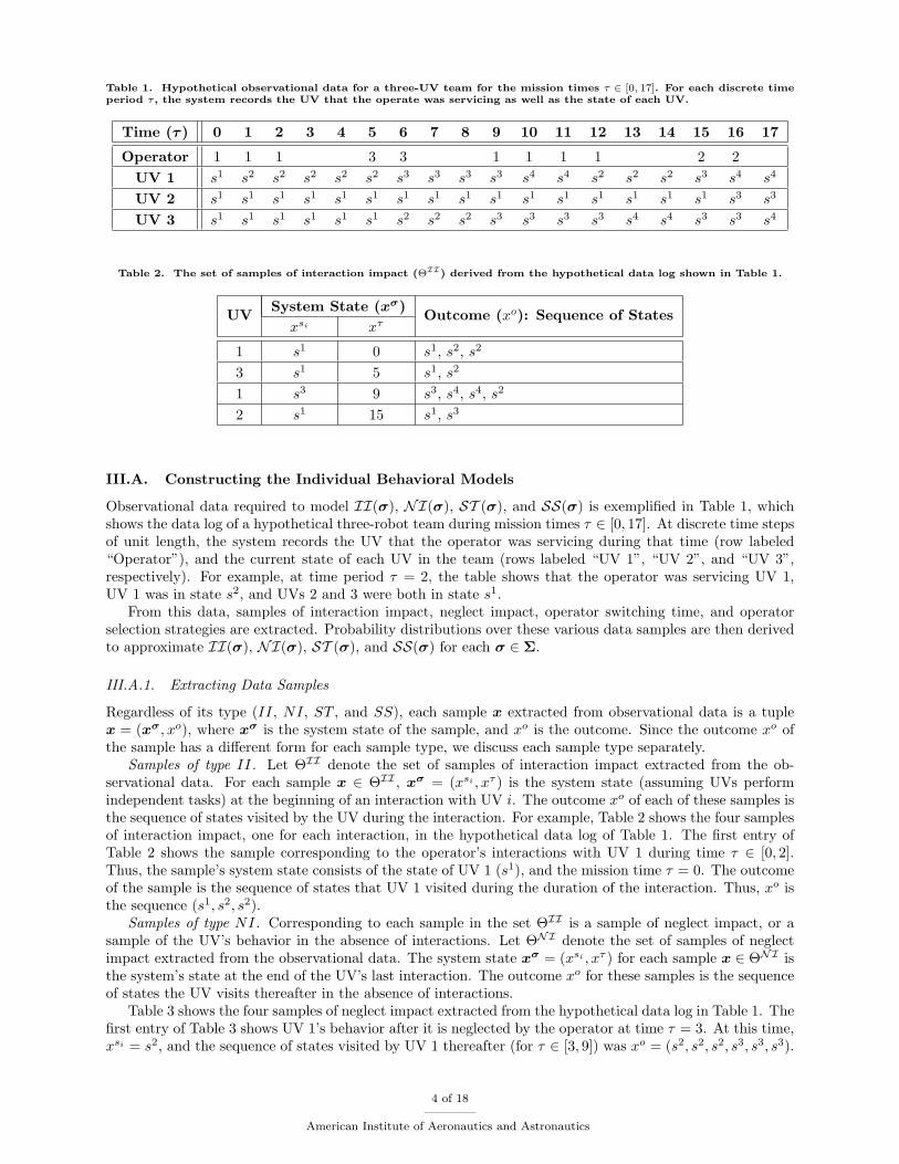
Table 1. Hypothetical observational data for a three-UV team for the mission times τ ∈ [0, 17]. For each discrete timeperiod τ , the system records the UV that the operate was servicing as well as the state of each UV.

Time (τ ) 0 1 2 3 4 5 6 7 8 9 10 11 12 13 14 15 16 17

Operator 1 1 1 3 3 1 1 1 1 2 2UV 1 s1 s2 s2 s2 s2 s2 s3 s3 s3 s3 s4 s4 s2 s2 s2 s3 s4 s4

UV 2 s1 s1 s1 s1 s1 s1 s1 s1 s1 s1 s1 s1 s1 s1 s1 s1 s3 s3

UV 3 s1 s1 s1 s1 s1 s1 s2 s2 s2 s3 s3 s3 s3 s4 s4 s3 s3 s4

Table 2. The set of samples of interaction impact (ΘII) derived from the hypothetical data log shown in Table 1.

UVSystem State (xσ)

Outcome (xo): Sequence of Statesxsi xτ

1 s1 0 s1, s2, s2

3 s1 5 s1, s2

1 s3 9 s3, s4, s4, s2

2 s1 15 s1, s3

III.A. Constructing the Individual Behavioral Models

Observational data required to model II(σ), NI(σ), ST (σ), and SS(σ) is exemplified in Table 1, whichshows the data log of a hypothetical three-robot team during mission times τ ∈ [0, 17]. At discrete time stepsof unit length, the system records the UV that the operator was servicing during that time (row labeled“Operator”), and the current state of each UV in the team (rows labeled “UV 1”, “UV 2”, and “UV 3”,respectively). For example, at time period τ = 2, the table shows that the operator was servicing UV 1,UV 1 was in state s2, and UVs 2 and 3 were both in state s1.

From this data, samples of interaction impact, neglect impact, operator switching time, and operatorselection strategies are extracted. Probability distributions over these various data samples are then derivedto approximate II(σ), NI(σ), ST (σ), and SS(σ) for each σ ∈ Σ.

III.A.1. Extracting Data Samples

Regardless of its type (II, NI, ST , and SS), each sample x extracted from observational data is a tuplex = (xσ, xo), where xσ is the system state of the sample, and xo is the outcome. Since the outcome xo ofthe sample has a different form for each sample type, we discuss each sample type separately.

Samples of type II. Let ΘII denote the set of samples of interaction impact extracted from the ob-servational data. For each sample x ∈ ΘII , xσ = (xsi , xτ ) is the system state (assuming UVs performindependent tasks) at the beginning of an interaction with UV i. The outcome xo of each of these samples isthe sequence of states visited by the UV during the interaction. For example, Table 2 shows the four samplesof interaction impact, one for each interaction, in the hypothetical data log of Table 1. The first entry ofTable 2 shows the sample corresponding to the operator’s interactions with UV 1 during time τ ∈ [0, 2].Thus, the sample’s system state consists of the state of UV 1 (s1), and the mission time τ = 0. The outcomeof the sample is the sequence of states that UV 1 visited during the duration of the interaction. Thus, xo isthe sequence (s1, s2, s2).

Samples of type NI. Corresponding to each sample in the set ΘII is a sample of neglect impact, or asample of the UV’s behavior in the absence of interactions. Let ΘNI denote the set of samples of neglectimpact extracted from the observational data. The system state xσ = (xsi , xτ ) for each sample x ∈ ΘNI isthe system’s state at the end of the UV’s last interaction. The outcome xo for these samples is the sequenceof states the UV visits thereafter in the absence of interactions.

Table 3 shows the four samples of neglect impact extracted from the hypothetical data log in Table 1. Thefirst entry of Table 3 shows UV 1’s behavior after it is neglected by the operator at time τ = 3. At this time,xsi = s2, and the sequence of states visited by UV 1 thereafter (for τ ∈ [3, 9]) was xo = (s2, s2, s2, s3, s3, s3).

4 of 18


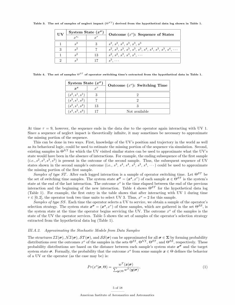
Table 3. The set of samples of neglect impact (ΘNI) derived from the hypothetical data log shown in Table 1.

UVSystem State (xσ)

Outcome (xo): Sequence of Statesxsi xτ

1 s2 3 s2, s2, s2, s3, s3, s3

3 s2 7 s2, s2, s3, s3, s3, s3, s4, s4, s3, s3, s4, · · ·1 s2 13 s2, s2, s3, s4, s4, · · ·2 s3 17 s3, · · ·

Table 4. The set of samples ΘST of operator switching time’s extracted from the hypothetical data in Table 1.

System State (xσ)Outcome (xo): Switching Time

xs xτ

(s2, s1, s1) 3 2(s3, s1, s2) 7 2(s2, s1, s4) 13 3(s4, s3, s4) 17 Not available

At time τ = 9, however, the sequence ends in the data due to the operator again interacting with UV 1.Since a sequence of neglect impact is theoretically infinite, it may sometimes be necessary to approximatethe missing portion of the sequence.

This can be done in two ways. First, knowledge of the UV’s position and trajectory in the world as wellas its behavioral logic, could be used to estimate the missing portion of the sequence via simulation. Second,existing samples in ΘNI for which the UV visited similar states can be used to approximate what the UV’sstate would have been in the absence of interactions. For example, the ending subsequence of the first sample(i.e., s2, s3, s3, s3) is present in the outcome of the second sample. Thus, the subsequent sequence of UVstates shown in the second sample’s outcome (i.e., s3, s4, s4, s3, s3, s4, · · · ) could be used to approximatethe missing portion of the first sample.

Samples of type ST . After each logged interaction is a sample of operator switching time. Let ΘST bethe set of switching time samples. The system state xσ = (xs, xτ ) of each sample x ∈ ΘST is the system’sstate at the end of the last interaction. The outcome xo is the time elapsed between the end of the previousinteraction and the beginning of the new interaction. Table 4 shows ΘST for the hypothetical data log(Table 1). For example, the first entry in the table shows that after interacting with UV 1 during timeτ ∈ [0, 2], the operator took two time units to select UV 3. Thus, xo = 2 for this sample.

Samples of type SS. Each time the operator selects a UV to service, we obtain a sample of the operator’sselection strategy. The system state xσ = (xs, xτ ) of these samples, which are gathered in the set ΘSS , isthe system state at the time the operator begins servicing the UV. The outcome xo of the samples is thestate of the UV the operator services. Table 5 shows the set of samples of the operator’s selection strategyextracted from the hypothetical data log (Table 1).

III.A.2. Approximating the Stochastic Models from Data Samples

The structures II(σ), NI(σ), ST (σ), and SS(σ) can be approximated for all σ ∈ Σ by forming probabilitydistributions over the outcomes xo of the samples in the sets ΘII , ΘNI , ΘST , and ΘSS , respectively. Theseprobability distributions are based on the distance between each sample’s system state xσ and the targetsystem state σ. Formally, the probability that the outcome xo from some sample x ∈ Θ defines the behaviorof a UV or the operator (as the case may be) is:

Pr(xo|σ,Θ) =wT (x|σ)∑y∈Θ w

T (y|σ), (1)

5 of 18


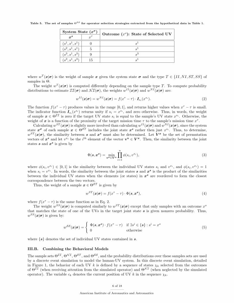
Table 5. The set of samples ΘSS for operator selection strategies extracted from the hypothetical data in Table 1.

System State (xσ)Outcome (xo): State of Selected UV

xs xτ

(s1, s1, s1) 0 s1

(s2, s1, s1) 5 s1

(s3, s1, s3) 9 s3

(s3, s1, s3) 15 s1

where wT (x|σ) is the weight of sample x given the system state σ and the type T ∈ {II,NI, ST, SS} ofsamples in Θ.

The weight wT (x|σ) is computed differently depending on the sample type T . To compute probabilitydistributions to estimate II(σ) and NI(σ), the weights wII(x|σ) and wNI(x|σ) are:

wII(x|σ) = wNI(x|σ) = f(xτ − τ) · Isi(xsi). (2)

The function f(xτ − τ) produces values in the range [0, 1], and returns higher values when xτ − τ is small.The indicator function Isi(x

si) returns unity if si = xsi , and zero otherwise. Thus, in words, the weightof sample x ∈ ΘII is zero if the target UV state si is equal to the sample’s UV state xsi . Otherwise, theweight of x is a function of the proximity of the target mission time τ to the sample’s mission time xτ .

Calculating wST (x|σ) is slightly more involved than calculating wII(x|σ) and wNI(x|σ), since the systemstate xσ of each sample x ∈ ΘST includes the joint state xs rather then just xsi . Thus, to determine,wST (x|σ), the similarity between s and xs must also be determined. Let V x be the set of permutationvectors of xs and let vxi be the ith element of the vector vx ∈ V x. Then, the similarity between the jointstates s and xs is given by

Φ(s,xs) = minvx∈V x

n∏i=1

φ(si, vxi), (3)

where φ(si, vxi) ∈ [0, 1] is the similarity between the individual UV states si and vxi , and φ(si, vxi) = 1when si = vxi . In words, the similarity between the joint states s and xs is the product of the similaritiesbetween the individual UV states when the elements (or states) in xs are reordered to form the closestcorrespondence between the two vectors.

Thus, the weight of a sample x ∈ ΘST is given by

wST (x|σ) = f(xτ − τ) · Φ(s,xs), (4)

where f(xτ − τ) is the same function as in Eq. 2.The weight wSS(x|σ) is computed similarly to wST (x|σ) except that only samples with an outcome xo

that matches the state of one of the UVs in the target joint state s is given nonzero probability. Thus,wSS(x|σ) is given by:

wSS(x|σ) =

{Φ(s,xs) · f(xτ − τ) if ∃si ∈ {s} : si = xo

0 otherwise(5)

where {s} denotes the set of individual UV states contained in s.

III.B. Combining the Behavioral Models

The sample sets ΘII , ΘNI , ΘST , and ΘSS , and the probability distributions over these samples sets are usedby a discrete event simulation to model the human-UV system. In this discrete event simulation, detailedin Figure 1, the behavior of each UV k is defined by a sequence of states χk selected from the outcomesof ΘII (when receiving attention from the simulated operator) and ΘNI (when neglected by the simulatedoperator). The variable ck denotes the current position of UV k in the sequence χk.

6 of 18


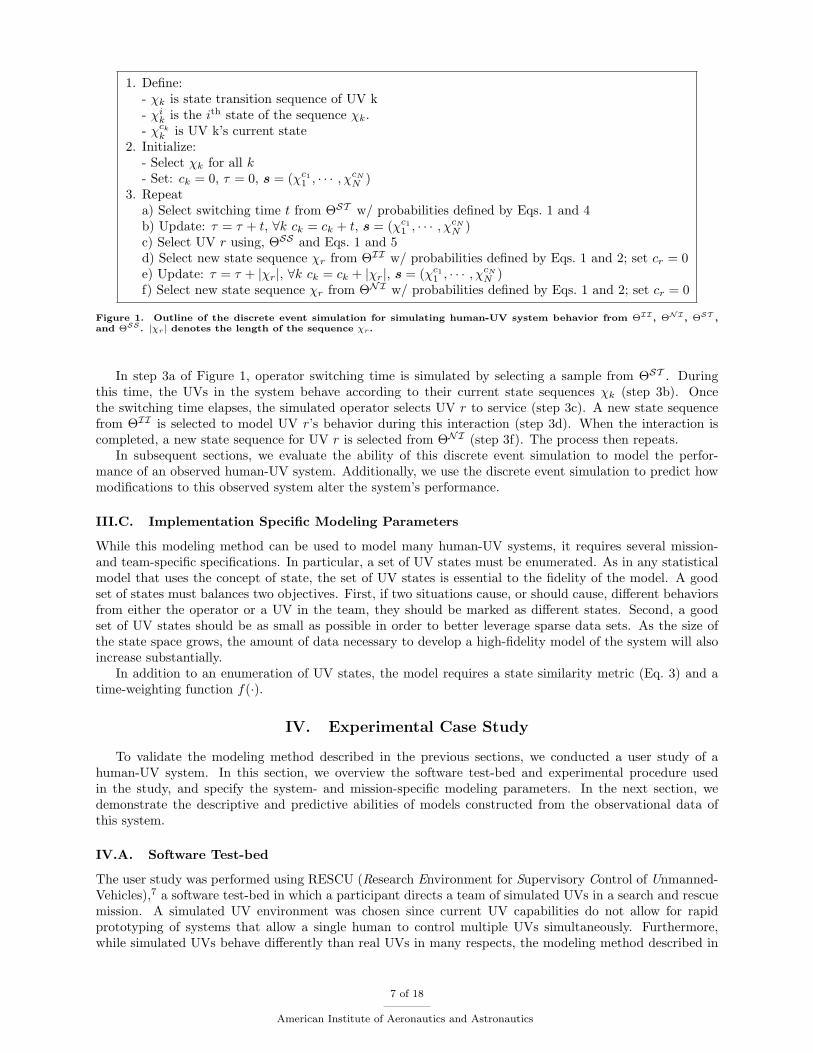
1. Define:- χk is state transition sequence of UV k- χik is the ith state of the sequence χk.- χckk is UV k’s current state

2. Initialize:- Select χk for all k- Set: ck = 0, τ = 0, s = (χc11 , · · · , χ

cNN )

3. Repeata) Select switching time t from ΘST w/ probabilities defined by Eqs. 1 and 4b) Update: τ = τ + t, ∀k ck = ck + t, s = (χc11 , · · · , χ

cNN )

c) Select UV r using, ΘSS and Eqs. 1 and 5d) Select new state sequence χr from ΘII w/ probabilities defined by Eqs. 1 and 2; set cr = 0e) Update: τ = τ + |χr|, ∀k ck = ck + |χr|, s = (χc11 , · · · , χ

cNN )

f) Select new state sequence χr from ΘNI w/ probabilities defined by Eqs. 1 and 2; set cr = 0

Figure 1. Outline of the discrete event simulation for simulating human-UV system behavior from ΘII, ΘNI, ΘST ,and ΘSS . |χr| denotes the length of the sequence χr.

In step 3a of Figure 1, operator switching time is simulated by selecting a sample from ΘST . Duringthis time, the UVs in the system behave according to their current state sequences χk (step 3b). Oncethe switching time elapses, the simulated operator selects UV r to service (step 3c). A new state sequencefrom ΘII is selected to model UV r’s behavior during this interaction (step 3d). When the interaction iscompleted, a new state sequence for UV r is selected from ΘNI (step 3f). The process then repeats.

In subsequent sections, we evaluate the ability of this discrete event simulation to model the perfor-mance of an observed human-UV system. Additionally, we use the discrete event simulation to predict howmodifications to this observed system alter the system’s performance.

III.C. Implementation Specific Modeling Parameters

While this modeling method can be used to model many human-UV systems, it requires several mission-and team-specific specifications. In particular, a set of UV states must be enumerated. As in any statisticalmodel that uses the concept of state, the set of UV states is essential to the fidelity of the model. A goodset of states must balances two objectives. First, if two situations cause, or should cause, different behaviorsfrom either the operator or a UV in the team, they should be marked as different states. Second, a goodset of UV states should be as small as possible in order to better leverage sparse data sets. As the size ofthe state space grows, the amount of data necessary to develop a high-fidelity model of the system will alsoincrease substantially.

In addition to an enumeration of UV states, the model requires a state similarity metric (Eq. 3) and atime-weighting function f(·).

IV. Experimental Case Study

To validate the modeling method described in the previous sections, we conducted a user study of ahuman-UV system. In this section, we overview the software test-bed and experimental procedure usedin the study, and specify the system- and mission-specific modeling parameters. In the next section, wedemonstrate the descriptive and predictive abilities of models constructed from the observational data ofthis system.

IV.A. Software Test-bed

The user study was performed using RESCU (Research Environment for Supervisory Control of Unmanned-Vehicles),7 a software test-bed in which a participant directs a team of simulated UVs in a search and rescuemission. A simulated UV environment was chosen since current UV capabilities do not allow for rapidprototyping of systems that allow a single human to control multiple UVs simultaneously. Furthermore,while simulated UVs behave differently than real UVs in many respects, the modeling method described in

7 of 18


this paper is the same regardless of whether UVs are simulated or real.We now overview RESCU in three parts: the team mission, the user interface, and the UVs’ behaviors.

Additional details about RESCU are provided in previous work.7

IV.A.1. Mission

Across many mission types, an operator of a human-UV system commonly assists in performing a set ofabstract tasks. These abstract tasks include mission planning and re-planning, UV path planning and re-planning, UV monitoring, sensor interpretation, and target designation. RESCU captures each of these tasksin a time-critical mission.

In RESCU, an operator (the study participant) directs a team of simulated UVs to collect objects froma building over an eight-minute time period. At the end of the eight minutes, the building “blows up,”destroying all UVs and objects left in it. Thus, in addition to collecting as many objects as possible, theoperator must also ensure that all UVs are out of the building when time expires. Specifically, operators areasked to maximize the following objective function:

Score = ObjectsCollected− UV sLost, (6)

where ObjectsCollected is the number of objects collected from the building during the session and UV sLostis the number of UVs remaining in the building when time expires.

An object is collected from the building using the following three-step process:

1. A UV moves to the location of an object in the building. This step requires the operator to beinvolved at some level in mission planning, target designation, path planning and re-planning, and UVmonitoring.

2. The UV picks up the object. In real-world systems, the operator would likely need to perform particulartasks to assist the UV in this process, such as identify the object from imagery. This burden on theoperator is emulated in RESCU by requiring the operator to find a U.S. city on a map.

3. The UV carries the object out of the building via one of two exits. This step requires the operator tomonitor the UV and assist in path planning and re-planning.

At the beginning of a RESCU mission, the UVs are positioned outside one of two entrances of thebuilding, and the objects are spread randomly throughout the building. The human-UV team can only seethe positions of six of the objects initially. In each minute of the session, the locations of two additionalobjects are revealed. Additionally, the map of the building is initially unknown. The UVs create a sharedmap of the building as they move about it.

IV.A.2. User Interface

The user interface for these RESCU experiments was the two-screen display shown in Figure 2. The mapof the building was displayed on the left screen, along with the positions of the UVs and the known objectsin the building. The right screen displayed the map of the United States operators used to locate cities toassist UVs in “picking up” objects. The operator controlled a single UV at a time, which he or she selectedby clicking a button on the interface corresponding to that UV. Once the operator selected the UV, he orshe directed the UV by designating a goal location and modifying the UV’s planned path to the goal. Todesignate a goal, the operator dragged the goal icon corresponding to the UV in question to the desiredlocation. The UV then generated and displayed the path it intended to follow. The operator could modifythis path with the mouse.

Two different interface modes were used. In the first mode, the operator was provided no assistance infinding U.S. cities on the map. This mode represents current UV systems in which operators must manuallyinterpret sensor information to identify and track objects and landmarks. In the second mode, the operatorwas assisted by an automated visioning system (AVS), designed to model potential real-world systems thatuse computer vision to help identify and track objects and landmarks from imagery. The AVS suggestedtwo cities to the operator by superimposing blinking red boxes on the map of the United States to mark thesuggested cities. The suggestions made by the AVS were correct about 70-75% of the time.

8 of 18


Figure 2. The RESCU user interface. The left display shows the UVs’ map of the building, as well as the locations ofthe objects, the UVs, and their destinations. The right display shows the map of the United States for locating cities.

IV.A.3. UV Behavior

The UVs used the well-known Dijkstra’s algorithm for path planning. However, since the map of the buildingwas incomplete, the UVs had to decide, using the techniques described in pervious work,7 between exploringthe unknown portions of the building and taking a known, possibly longer, path. The resulting path planningalgorithm allowed the UVs to effectively traverse the building in most situations. However, as in real-worldsystems, UV behavior was not always ideal. As a result, operators sometimes found it necessary to correctthe UV’s plans and actions.

Two different UV autonomy modes were used in the study. In the first mode, the operator manuallyassigned all UV goal destinations. If the operator did not provide a goal for a UV, it remained idle and didnot move. This mode represents the current state-of-the-art, in which the UV used autonomous capabilities,such as “fly-by-wire” technologies, to navigate to human-designated locations. In the second mode, whichrepresents potential UV capabilities of the future, a UV automatically selected its own goal destination insome situations. The UVs used the following rules for generating goal destinations:

1. An idle UV that was carrying an object automatically selected the nearest perceived exit for its goaldestination.

2. An idle UV not carrying an object automatically selected the nearest perceived unassigned object forits goal destination.

3. In the last minute of the session, each UV automatically selected the nearest perceived exit for its goaldestination.

A management-by-exception (MBE) level of automation2 was used to allow the operator to over-rule theselections made by the UVs. The UV waited 15 seconds before executing the selection to allow the operatorto override it. We refer to this mode as MBE autonomy.

IV.B. Experimental Procedure

The experiment was a 4 (decision support) x 4 (UV team size) mixed design study. Decision support wasa between-subjects factor, where each participant was assigned a specific level. The four levels of decisionsupport were:

1. noDS – The human-UV system was not equipped with the AVS or MBE autonomy.

2. AVS – The human-UV system was equipped with the AVS but not MBE autonomy.

3. MBE – The human-UV system was equipped with MBE autonomy but not the AVS.

4. AVS-MBE – The human-UV system was equipped with the AVS and MBE autonomy.

9 of 18


"Pick up" or Assign (or near)

Assign "Pick up" Obscured PathClear Path

ArrivedAlmostArrived

ExploringKnownPathExploring

CarryingObject

CarryingObject

NotCarryingObject

NotCarryingObject

CarryingObject

NotCarryingObject

KnownPath

UnknownPath

BestGoal

s1 s2 s3 s4 s5

UnknownPath

Sub−optimalGoal

BestGoal

Sub−optimalGoal

KnownPath

UnknownPath

UnknownPath

Searching

KnownPath

KnownPath

UnknownPath

UnknownPath

s6 s7

ArrivedAlmostArrived

Engaged

s8 s9 s11s10 s12 s13 s14 s15 s16 s17 s18 s19 s20 s21 s22

Exiting Building

OutsideBuilding

InsideBuilding

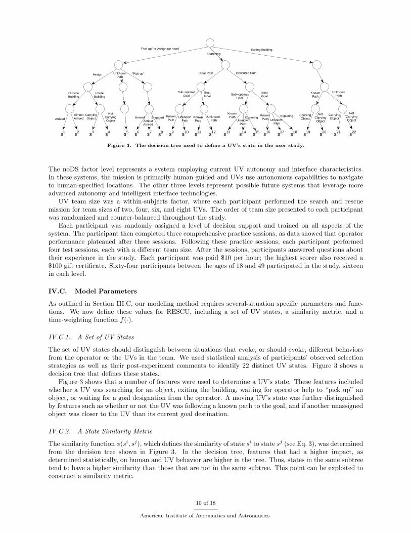
Figure 3. The decision tree used to define a UV’s state in the user study.

The noDS factor level represents a system employing current UV autonomy and interface characteristics.In these systems, the mission is primarily human-guided and UVs use autonomous capabilities to navigateto human-specified locations. The other three levels represent possible future systems that leverage moreadvanced autonomy and intelligent interface technologies.

UV team size was a within-subjects factor, where each participant performed the search and rescuemission for team sizes of two, four, six, and eight UVs. The order of team size presented to each participantwas randomized and counter-balanced throughout the study.

Each participant was randomly assigned a level of decision support and trained on all aspects of thesystem. The participant then completed three comprehensive practice sessions, as data showed that operatorperformance plateaued after three sessions. Following these practice sessions, each participant performedfour test sessions, each with a different team size. After the sessions, participants answered questions abouttheir experience in the study. Each participant was paid $10 per hour; the highest scorer also received a$100 gift certificate. Sixty-four participants between the ages of 18 and 49 participated in the study, sixteenin each level.

IV.C. Model Parameters

As outlined in Section III.C, our modeling method requires several-situation specific parameters and func-tions. We now define these values for RESCU, including a set of UV states, a similarity metric, and atime-weighting function f(·).

IV.C.1. A Set of UV States

The set of UV states should distinguish between situations that evoke, or should evoke, different behaviorsfrom the operator or the UVs in the team. We used statistical analysis of participants’ observed selectionstrategies as well as their post-experiment comments to identify 22 distinct UV states. Figure 3 shows adecision tree that defines these states.

Figure 3 shows that a number of features were used to determine a UV’s state. These features includedwhether a UV was searching for an object, exiting the building, waiting for operator help to “pick up” anobject, or waiting for a goal designation from the operator. A moving UV’s state was further distinguishedby features such as whether or not the UV was following a known path to the goal, and if another unassignedobject was closer to the UV than its current goal destination.

IV.C.2. A State Similarity Metric

The similarity function φ(si, sj), which defines the similarity of state si to state sj (see Eq. 3), was determinedfrom the decision tree shown in Figure 3. In the decision tree, features that had a higher impact, asdetermined statistically, on human and UV behavior are higher in the tree. Thus, states in the same subtreetend to have a higher similarity than those that are not in the same subtree. This point can be exploited toconstruct a similarity metric.

10 of 18


Formally, let g(si, sj) denote the length of the path in the decision tree from si to the nearest commonancestor of si and sj . For example, g(s1, s2) = 1 since the states s1 and s2 share the same parent, whereas,g(s1, s5) = 3 since the nearest common ancestor is three levels up the tree. Then, φ(si, sj) is given by

φ(si, sj) =1

g(si, sj)c, (7)

where c is some positive integer that controls the sensitivity of the metric. Increasing c decreases thesimilarities between states.

IV.C.3. A Time-Weighting Function f(·)

Recall that the time-weighting function f(·) is used to weight a sample based on mission time. We use afunction proportional to a truncated Gaussian for f(·), namely

f(xτ − τ) =

{exp

(− (xτ−τ)2

2ν2

)if (xτ − τ) < W

0 otherwise(8)

where ν and W are positive constants. Due to the time-critical nature of RESCU, we chose to truncate theGaussian function (with W ) so that a sample’s weight was positive only if xτ was close to τ .

V. Results

In this section, we discuss the results of the user study and use these results to evaluate our modelingmethod’s ability to describe and predict the performance of human-UV systems. We first summarize theobserved performance of the various human-UV systems observed in the user study. Next, we model thenoDS human-UV systems using observational data from subjects that commanded the noDS systems in thestudy. Finally, we predict the performance of the AVS, MBE, and AVS-MBE systems from these models,and compare these predictions to the observed results in the study.

V.A. Observed System Performance

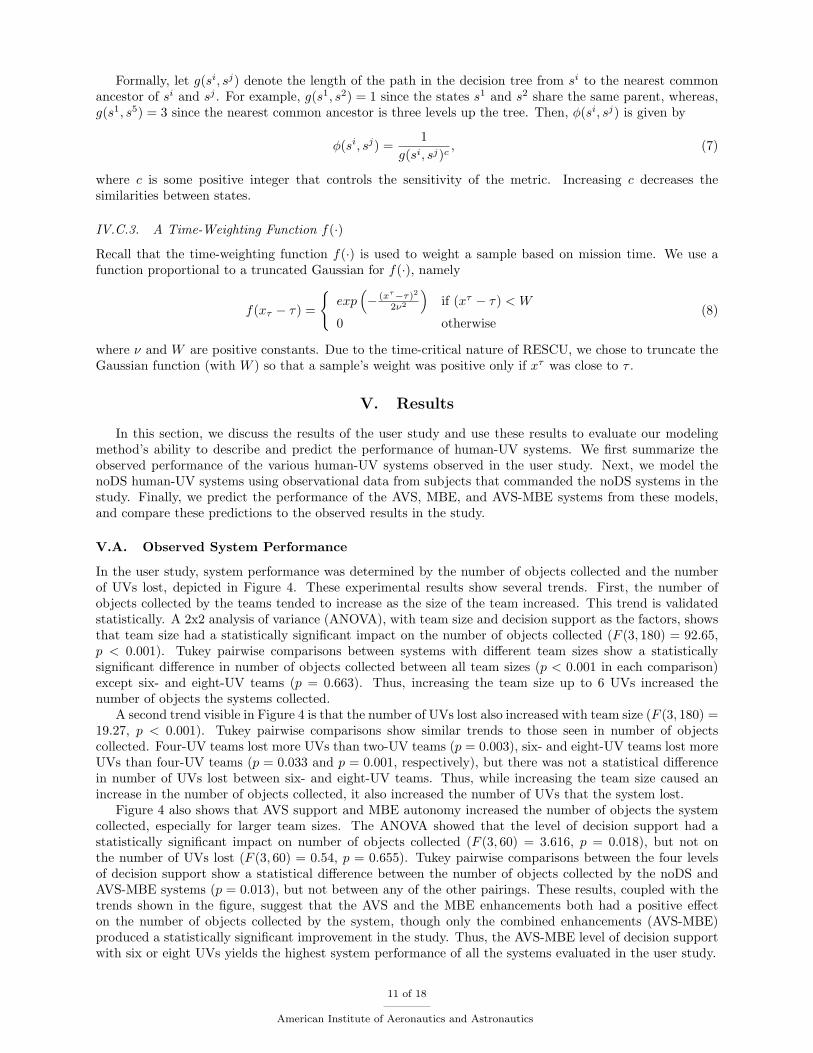
In the user study, system performance was determined by the number of objects collected and the numberof UVs lost, depicted in Figure 4. These experimental results show several trends. First, the number ofobjects collected by the teams tended to increase as the size of the team increased. This trend is validatedstatistically. A 2x2 analysis of variance (ANOVA), with team size and decision support as the factors, showsthat team size had a statistically significant impact on the number of objects collected (F (3, 180) = 92.65,p < 0.001). Tukey pairwise comparisons between systems with different team sizes show a statisticallysignificant difference in number of objects collected between all team sizes (p < 0.001 in each comparison)except six- and eight-UV teams (p = 0.663). Thus, increasing the team size up to 6 UVs increased thenumber of objects the systems collected.

A second trend visible in Figure 4 is that the number of UVs lost also increased with team size (F (3, 180) =19.27, p < 0.001). Tukey pairwise comparisons show similar trends to those seen in number of objectscollected. Four-UV teams lost more UVs than two-UV teams (p = 0.003), six- and eight-UV teams lost moreUVs than four-UV teams (p = 0.033 and p = 0.001, respectively), but there was not a statistical differencein number of UVs lost between six- and eight-UV teams. Thus, while increasing the team size caused anincrease in the number of objects collected, it also increased the number of UVs that the system lost.

Figure 4 also shows that AVS support and MBE autonomy increased the number of objects the systemcollected, especially for larger team sizes. The ANOVA showed that the level of decision support had astatistically significant impact on number of objects collected (F (3, 60) = 3.616, p = 0.018), but not onthe number of UVs lost (F (3, 60) = 0.54, p = 0.655). Tukey pairwise comparisons between the four levelsof decision support show a statistical difference between the number of objects collected by the noDS andAVS-MBE systems (p = 0.013), but not between any of the other pairings. These results, coupled with thetrends shown in the figure, suggest that the AVS and the MBE enhancements both had a positive effecton the number of objects collected by the system, though only the combined enhancements (AVS-MBE)produced a statistically significant improvement in the study. Thus, the AVS-MBE level of decision supportwith six or eight UVs yields the highest system performance of all the systems evaluated in the user study.

11 of 18


2 4 6 8

7

8

9

10

11

12

13

14

15

# of UVs

Obj

ects

Col

lect

ed

noDS (observed)AVS (observed)MBE (observed)AVS−MBE (observed)

2 4 6 80

0.5

1

1.5

2

2.5

# of UVs

UV

s Lo

st

noDS (observed)AVS (observed)MBE (observed)AVS−MBE (observed)

Figure 4. Mean number of objects collected (left) and UVs lost (right) observed in each experimental condition.

2 4 6 8

7

8

9

10

11

12

# of UVs

Obj

ects

Col

lect

ed

noDS (observed)Modeled

2 4 6 80

0.5

1

1.5

2

2.5

3

3.5

# of UVs

UV

s Lo

st

noDS (observed)Modeled

Figure 5. Comparison of observed performance of the noDS human-UV systems to model estimates of objects collected(left) and UVs lost (right). Error bars represent a 95% confidence interval on the mean.

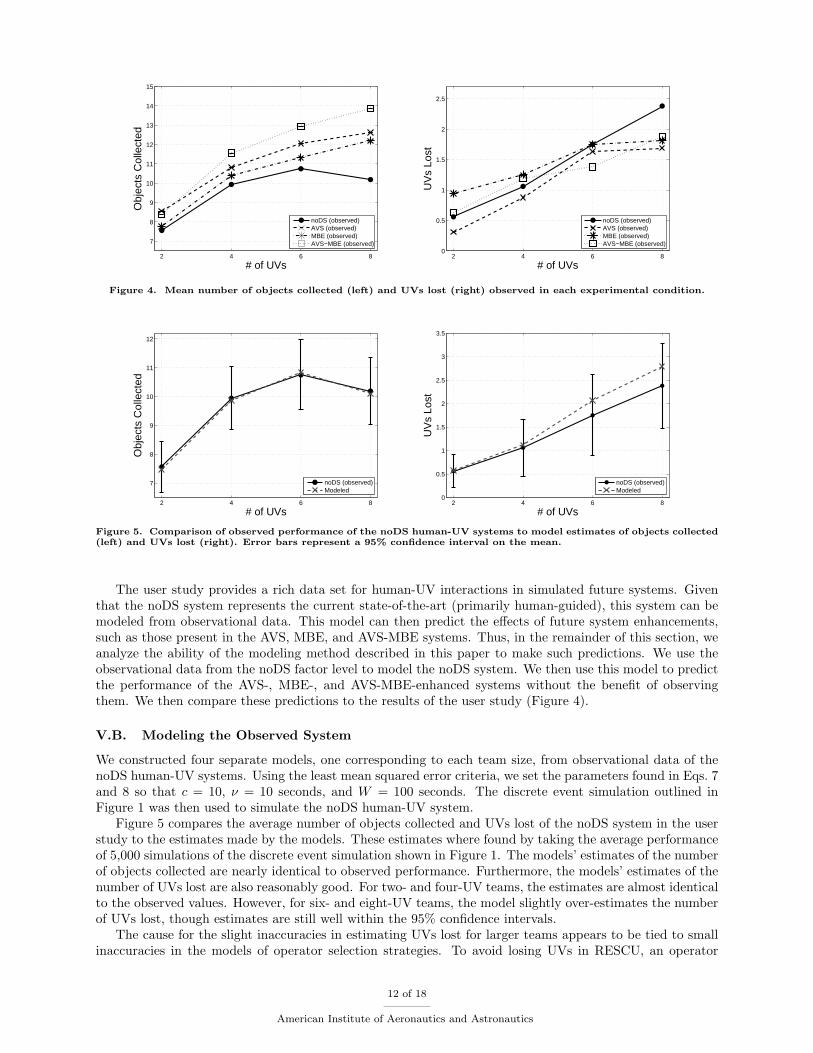
The user study provides a rich data set for human-UV interactions in simulated future systems. Giventhat the noDS system represents the current state-of-the-art (primarily human-guided), this system can bemodeled from observational data. This model can then predict the effects of future system enhancements,such as those present in the AVS, MBE, and AVS-MBE systems. Thus, in the remainder of this section, weanalyze the ability of the modeling method described in this paper to make such predictions. We use theobservational data from the noDS factor level to model the noDS system. We then use this model to predictthe performance of the AVS-, MBE-, and AVS-MBE-enhanced systems without the benefit of observingthem. We then compare these predictions to the results of the user study (Figure 4).

V.B. Modeling the Observed System

We constructed four separate models, one corresponding to each team size, from observational data of thenoDS human-UV systems. Using the least mean squared error criteria, we set the parameters found in Eqs. 7and 8 so that c = 10, ν = 10 seconds, and W = 100 seconds. The discrete event simulation outlined inFigure 1 was then used to simulate the noDS human-UV system.

Figure 5 compares the average number of objects collected and UVs lost of the noDS system in the userstudy to the estimates made by the models. These estimates where found by taking the average performanceof 5,000 simulations of the discrete event simulation shown in Figure 1. The models’ estimates of the numberof objects collected are nearly identical to observed performance. Furthermore, the models’ estimates of thenumber of UVs lost are also reasonably good. For two- and four-UV teams, the estimates are almost identicalto the observed values. However, for six- and eight-UV teams, the model slightly over-estimates the numberof UVs lost, though estimates are still well within the 95% confidence intervals.

The cause for the slight inaccuracies in estimating UVs lost for larger teams appears to be tied to smallinaccuracies in the models of operator selection strategies. To avoid losing UVs in RESCU, an operator

12 of 18


is sometimes required to make precise time-critical decisions in order to ensure that UVs exit the buildingbefore time expires, whereas the same time-critical precision is not required to collect objects. As the jointstate space becomes larger with larger teams, the relatively small number of data samples compared to thesize of the joint state space makes it difficult to model operator strategies with sufficient precision. As aresult, the model slightly over-estimates the number of UVs lost in larger UV teams.

Despite these small inaccuracies, the estimates are, overall, reasonably good. The models effectivelydescribe the observed system. However, these results do not demonstrate predictive ability since the modelis only duplicating observed results. To be predictive, the model must be able to predict the performance ofunobserved systems.

V.C. Predicting the Effects of System Design Modifications

We now evaluate the models’ ability to predict the performance of the system with the AVS, MBE, andAVS-MBE enhancements.

V.C.1. Predicting the Effects of the AVS Support

To predict how the AVS enhancement would change system performance, we must determine the aspectsof the team that would be affected by the AVS and how they would be changed. These changes must bereflected in the individual samples, which entails either deriving a new set of samples, or editing the existingsamples. We use the latter approach in this paper.

Since the AVS affects human-UV interactions, it will mostly affect II; we assume that the other aspectsof the system are left unchanged. To capture the change in II induced by the AVS enhancement, we editthe outcome xo of each sample x ∈ ΘII in which the operator assisted a UV in “picking up” on object bylocating a city on the map of the United States. In these samples, the amount of time taken to identify thecity should be altered to reflect the change induced by the AVS support.

For example, consider the following outcome of a hypothetical sample of interaction impact:

s6, s6, s6, s8, s8, s8, s8, s8, s8, s8, s8, s8, s8, s8, s3, s3, s3, s18, s18

From the state tree shown in Figure 3, we can deduce that state s8 corresponds to situations in which theoperator and UV are engaged in “picking up” an object. In the state transition sequence, this process takeseleven time units, beginning with the 4th element of the sequence and ending with the 14th element of thesequence. To estimate the effects of the AVS support, we remove this subsequence and replace it with asubsequence reflecting the amount of time the process would take with the AVS support. For example, ifwe have cause to believe that it would take the operator just six time units with the AVS support, then theedited sequence would be:

s6, s6, s6, s8, s8, s8, s8, s8, s8, s3, s3, s3, s18, s18.

Note, however, that since the effects of the AVS support are not completely known a priori, we mustestimate what they might be, or evaluate the proposed automated visioning system. We estimated the lengthof time it takes operators to locate a city in a separate evaluation of the AVS support, and substituted thesetimes into the appropriate samples in ΘII . On average, we observed that the AVS support reduced the timeit took operators to locate the city by approximately five seconds.

After editing the samples in this way, we simulated the AVS-enhanced system using the discrete eventsimulation outlined in Figure 1. We then adjusted the simulation’s predictions of system performance toaccount for the initial errors present in the model. Specifically, we multiplied the simulation’s predictions bythe ratio of the observed values to the model estimates in Figure 5. The resulting predictions are comparedto the observed performance in the user study in Figure 6. For each team size, the predictions are reasonablyaccurate for both number of objects collected and UVs lost, as all predictions fall within the 95% confidenceintervals. Thus, the models effectively predicted the affects of the AVS enhancement.

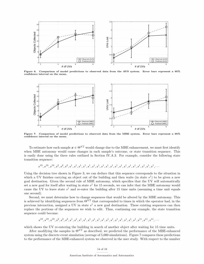
V.C.2. Predicting the Effects of the MBE Autonomy

The MBE autonomy alters a UV’s behavior in the absence of interactions. Thus, whereas the AVS supportprimarily affected II, the MBE autonomy primarily affects NI. As such, to simulate the effects of the MBEautonomy, we must modify the samples in ΘNI to reflect this new behavior.

13 of 18


2 4 6 87

8

9

10

11

12

13

14

# of UVs

Obj

ects

Col

lect

ed

Observed (AVS)Predicted (AVS)

2 4 6 80

0.5

1

1.5

2

2.5

# of UVs

UV

s Lo

st

Observed (AVS)Predicted (AVS)

Figure 6. Comparison of model predictions to observed data from the AVS system. Error bars represent a 95%confidence interval on the mean.

2 4 6 86

7

8

9

10

11

12

13

14

# of UVs

Obj

ects

Col

lect

ed

Observed (MBE)Predicted (MBE)

2 4 6 80

0.5

1

1.5

2

2.5

3

# of UVs

UV

s Lo

st

Observed (MBE)Predicted (MBE)

Figure 7. Comparison of model predictions to observed data from the MBE system. Error bars represent a 95%confidence interval on the mean.

To estimate how each sample x ∈ ΘNI would change due to the MBE enhancement, we must first identifywhen MBE autonomy would cause changes in each sample’s outcome, or state transition sequence. Thisis easily done using the three rules outlined in Section IV.A.3. For example, consider the following statetransition sequence:

s19, s19, s19, s2, s2, s2, s1, s1, s1, s1, s1, s1, s1, s1, s1, s1, s1, s1, s1, s1, s1, s1, s1, s1, s1, · · ·

Using the decision tree shown in Figure 3, we can deduce that this sequence corresponds to the situation inwhich a UV finishes carrying an object out of the building and then waits (in state s1) to be given a newgoal destination. Given the second rule of MBE autonomy, which specifies that the UV will automaticallyset a new goal for itself after waiting in state s1 for 15 seconds, we can infer that the MBE autonomy wouldcause the UV to leave state s1 and re-enter the building after 15 time units (assuming a time unit equalsone second).

Second, we must determine how to change sequences that would be altered by the MBE autonomy. Thisis achieved by identifying sequences from ΘNI that corresponded to times in which the operator had, in theprevious interaction, assigned a UV in state s1 a new goal destination. These existing sequences can thenreplace the portions of the sequences we wish to edit. Thus, continuing our example, the state transitionsequence could become:

s19, s19, s19, s2, s2, s2, s1, s1, s1, s1, s1, s1, s1, s1, s1, s1, s1, s1, s1, s1, s1, s11, s11, s11, · · ·

which shows the UV re-entering the building in search of another object after waiting for 15 time units.After modifying the samples in ΘNI as described, we predicted the performance of the MBE-enhanced

system using the discrete event simulation (average of 5,000 simulations). Figure 7 compares these predictionsto the performance of the MBE-enhanced system we observed in the user study. With respect to the number

14 of 18


2 4 6 87

8

9

10

11

12

13

14

15

16

# of UVs

Obj

ects

Col

lect

ed

Observed (AVS−MBE)Predicted(AVS−MBE)

2 4 6 80

0.5

1

1.5

2

2.5

3

# of UVs

UV

s Lo

st

Observed (AVS−MBE)Predicted (AVS−MBE)

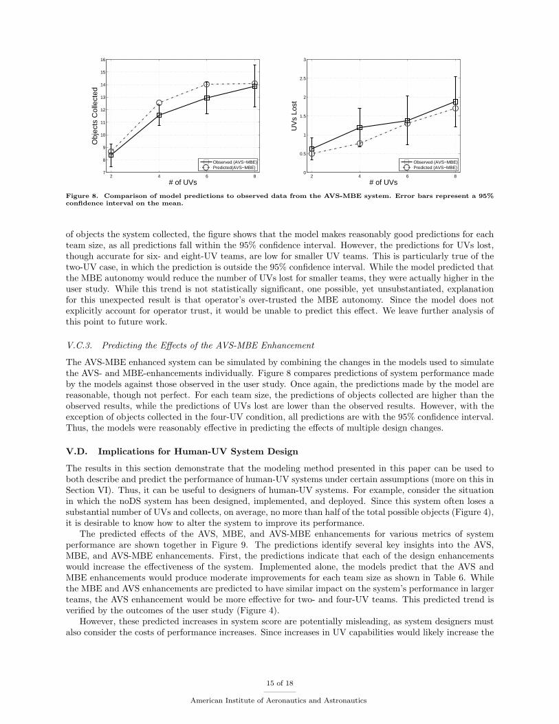
Figure 8. Comparison of model predictions to observed data from the AVS-MBE system. Error bars represent a 95%confidence interval on the mean.

of objects the system collected, the figure shows that the model makes reasonably good predictions for eachteam size, as all predictions fall within the 95% confidence interval. However, the predictions for UVs lost,though accurate for six- and eight-UV teams, are low for smaller UV teams. This is particularly true of thetwo-UV case, in which the prediction is outside the 95% confidence interval. While the model predicted thatthe MBE autonomy would reduce the number of UVs lost for smaller teams, they were actually higher in theuser study. While this trend is not statistically significant, one possible, yet unsubstantiated, explanationfor this unexpected result is that operator’s over-trusted the MBE autonomy. Since the model does notexplicitly account for operator trust, it would be unable to predict this effect. We leave further analysis ofthis point to future work.

V.C.3. Predicting the Effects of the AVS-MBE Enhancement

The AVS-MBE enhanced system can be simulated by combining the changes in the models used to simulatethe AVS- and MBE-enhancements individually. Figure 8 compares predictions of system performance madeby the models against those observed in the user study. Once again, the predictions made by the model arereasonable, though not perfect. For each team size, the predictions of objects collected are higher than theobserved results, while the predictions of UVs lost are lower than the observed results. However, with theexception of objects collected in the four-UV condition, all predictions are with the 95% confidence interval.Thus, the models were reasonably effective in predicting the effects of multiple design changes.

V.D. Implications for Human-UV System Design

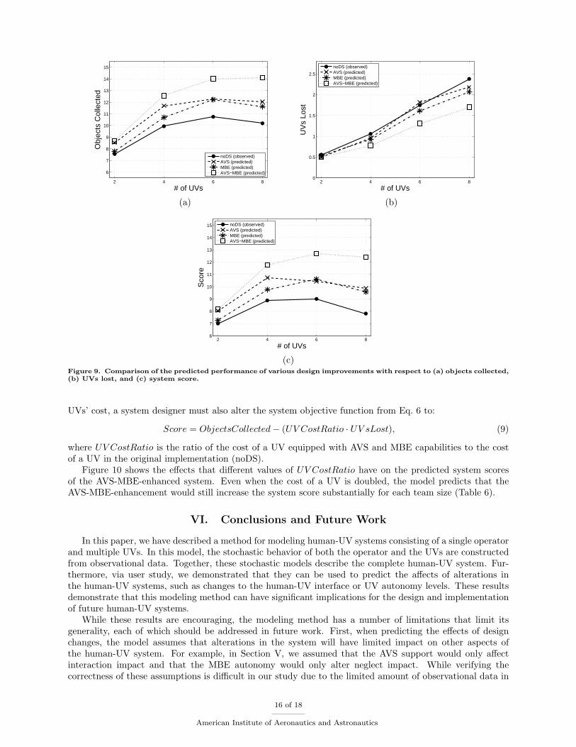
The results in this section demonstrate that the modeling method presented in this paper can be used toboth describe and predict the performance of human-UV systems under certain assumptions (more on this inSection VI). Thus, it can be useful to designers of human-UV systems. For example, consider the situationin which the noDS system has been designed, implemented, and deployed. Since this system often loses asubstantial number of UVs and collects, on average, no more than half of the total possible objects (Figure 4),it is desirable to know how to alter the system to improve its performance.

The predicted effects of the AVS, MBE, and AVS-MBE enhancements for various metrics of systemperformance are shown together in Figure 9. The predictions identify several key insights into the AVS,MBE, and AVS-MBE enhancements. First, the predictions indicate that each of the design enhancementswould increase the effectiveness of the system. Implemented alone, the models predict that the AVS andMBE enhancements would produce moderate improvements for each team size as shown in Table 6. Whilethe MBE and AVS enhancements are predicted to have similar impact on the system’s performance in largerteams, the AVS enhancement would be more effective for two- and four-UV teams. This predicted trend isverified by the outcomes of the user study (Figure 4).

However, these predicted increases in system score are potentially misleading, as system designers mustalso consider the costs of performance increases. Since increases in UV capabilities would likely increase the

15 of 18


2 4 6 8

6

7

8

9

10

11

12

13

14

15

# of UVs

Obj

ects

Col

lect

ed

noDS (observed)AVS (predicted)MBE (predicted)AVS−MBE (predicted)

2 4 6 80

0.5

1

1.5

2

2.5

# of UVs

UV

s Lo

st


(a) (b)

2 4 6 86

7

8

9

10

11

12

13

14

15

# of UVs

Sco

re


(c)Figure 9. Comparison of the predicted performance of various design improvements with respect to (a) objects collected,(b) UVs lost, and (c) system score.

UVs’ cost, a system designer must also alter the system objective function from Eq. 6 to:

Score = ObjectsCollected− (UV CostRatio · UV sLost), (9)

where UV CostRatio is the ratio of the cost of a UV equipped with AVS and MBE capabilities to the costof a UV in the original implementation (noDS).

Figure 10 shows the effects that different values of UV CostRatio have on the predicted system scoresof the AVS-MBE-enhanced system. Even when the cost of a UV is doubled, the model predicts that theAVS-MBE-enhancement would still increase the system score substantially for each team size (Table 6).

VI. Conclusions and Future Work

In this paper, we have described a method for modeling human-UV systems consisting of a single operatorand multiple UVs. In this model, the stochastic behavior of both the operator and the UVs are constructedfrom observational data. Together, these stochastic models describe the complete human-UV system. Fur-thermore, via user study, we demonstrated that they can be used to predict the affects of alterations inthe human-UV systems, such as changes to the human-UV interface or UV autonomy levels. These resultsdemonstrate that this modeling method can have significant implications for the design and implementationof future human-UV systems.

While these results are encouraging, the modeling method has a number of limitations that limit itsgenerality, each of which should be addressed in future work. First, when predicting the effects of designchanges, the model assumes that alterations in the system will have limited impact on other aspects ofthe human-UV system. For example, in Section V, we assumed that the AVS support would only affectinteraction impact and that the MBE autonomy would only alter neglect impact. While verifying thecorrectness of these assumptions is difficult in our study due to the limited amount of observational data in

16 of 18


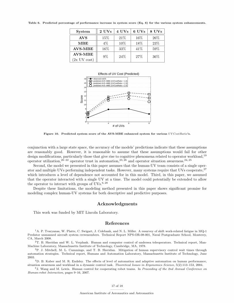
Table 6. Predicted percentage of performance increase in system score (Eq. 6) for the various system enhancements.

System 2 UVs 4 UVs 6 UVs 8 UVs

AVS 15% 21% 16% 26%MBE 4% 10% 18% 23%

AVS-MBE 16% 33% 41% 59%AVS-MBE 9% 24% 27% 36%(2x UV cost)

2 4 6 86

7

8

9

10

11

12

13

14

15

16

# of UVs

Sco

re

Effects of UV Cost (Predicted)

observed noDSpredicted AVS−MBE (UVCostRatio = 1.0)predicted AVS−MBE (UVCostRatio = 1.5)predicted AVS−MBE (UVCostRatio = 2.0)

Figure 10. Predicted system score of the AVS-MBE enhanced system for various UV CostRatio’s.

conjunction with a large state space, the accuracy of the models’ predictions indicate that these assumptionsare reasonably good. However, it is reasonable to assume that these assumptions would fail for otherdesign modifications, particularly those that give rise to cognitive phenomena related to operator workload,19

operator utilization,20–22 operator trust in automation,23,26 and operator situation awareness.24,25

Second, the model we presented in this paper assumes that the human-UV team consists of a single oper-ator and multiple UVs performing independent tasks. However, many systems require that UVs cooperate,27

which introduces a level of dependence not accounted for in this model. Third, in this paper, we assumedthat the operator interacted with a single UV at a time. The model could potentially be extended to allowthe operator to interact with groups of UVs.6,28

Despite these limitations, the modeling method presented in this paper shows significant promise formodeling complex human-UV systems for both descriptive and predictive purposes.

Acknowledgments

This work was funded by MIT Lincoln Laboratory.

References

1A. P. Tvaryanas, W. Platte, C. Swigart, J. Colebank, and N. L. Miller. A resurvey of shift work-related fatigue in MQ-1Predator unmanned aircraft system crewmembers. Technical Report NPS-OR-08-001, Naval Postgraduate School, Monterey,CA, March 2008.

2T. B. Sheridan and W. L. Verplank. Human and computer control of undersea teleoperators. Technical report, Man-Machine Laboratory, Massachusetts Institute of Technology, Cambridge, MA, 1978.

3P. J. Mitchell, M. L. Cummings, and T. B. Sheridan. Mitigation of human supervisory control wait times throughautomation strategies. Technical report, Humans and Automation Laboratory, Massachusetts Institute of Technology, June2003.

4D. B. Kaber and M. R. Endsley. The effects of level of automation and adaptive automation on human performance,situation awareness and workload in a dynamic control task. Theoretical Issues in Ergonomics Science, 5(2):113–153, 2004.

5J. Wang and M. Lewis. Human control for cooperating robot teams. In Proceeding of the 2nd Annual Conference onHuman-robot Interaction, pages 9–16, 2007.

17 of 18


6M. A. Goodrich, T. W. McLain, J. D. Anderson, J. Sun, and J. W. Crandall. Managing autonomy in robot teams:observations from four experiments. In Proceeding of the 2nd Annual Conference on Human-robot Interaction, pages 25–32,2007.

7J. W. Crandall and M. L. Cummings. Identifying predictive metrics for supervisory control of multiple robots. IEEETransactions on Robotics, 23(5), October 2007.

8M. A. Goodrich, D. R. Olsen Jr, J. W. Crandall, and T. J. Palmer. Experiments in adjustable autonomy. In Proceedingsof IJCAI Workshop on Autonomy, Delegation and Control: Interacting with Intelligent Agents, 2001.

9D. R. Olsen Jr. and S. B. Wood. Fan-out: Measuring human control of multiple robots. In Proceedings of the Conferenceon Human Factors in Computing Systems, 2004.

10J. W. Crandall, M. A. Goodrich, D. R. Olsen Jr., and C. W. Nielsen. Validating human-robot systems in multi-taskingenvironments. IEEE Transactions on Systems, Man, and Cybernetics – Part A: Systems and Humans, 35(4):438–449, 2005.

11D. R. Olsen Jr. and M. A. Goodrich. Metrics for evaluating human-robot interactions. In NIST’s Performance Metricsfor Intelligent Systems Workshop, Gaithersburg, MA, 2003.

12T. B. Sheridan and M. K. Tulga. A model for dynamic allocation of human attention among multiple tasks. In Proceedingsof the 14th Annual Conference on Manual Control, 1978.

13S. Mau and J. Dolan. Scheduling to minimize downtime in human-multirobot supervisory control. In Workshop onPlanning and Scheduling for Space, 2006.

14H. Neth, S. S. Khemlani, B. Oppermann, and W. D. Gray. Juggling multiple tasks: A rational analysis of multitaskingin a synthetic task environment. In Proceedings of the 50th Annual Meeting of the Human Factors and Ergonomics Society,2006.

15P. Squire, G. Trafton, and R. Parasuraman. Human control of multiple unmanned vehicles: effects of interface type onexecution and task switching times. In Proceeding of the 1st Annual Conference on Human-robot Interaction, pages 26–32,New York, NY, USA, 2006. ACM Press.

16M. A. Goodrich, M. Quigley, and K. Cosenzo. Task switching and multi-robot teams. In Proceedings of the ThirdInternational Multi-Robot Systems Workshop, 2005.

17M. L. Cummings and P. J. Mitchell. Predicting controller capacity in remote supervision of multiple unmanned vehicles.IEEE Transactions on Systems, Man, and Cybernetics – Part A Systems and Humans, 38(2):451–460, 2008.

18M. L. Cummings, C. Nehme, J. W. Crandall, and P. J. Mitchell. Predicting operator capacity for supervisory control ofmultiple UAVs. Innovations in Intelligent UAVs: Theory and Applications, Ed. L. Jain, 2007.

19R. M. Yerkes and J. D. Dodson. The relation of strength of stimulus to rapidity of habit-formation. Journal of ComparativeNeurology and Psychology, 18:459–482, 1908.

20D. K. Schmidt. A queuing analysis of the air traffic controller’s workload. IEEE Transactions on Systems, Man, andCybernetics, 8(6):492–498, 1978.

21W. B. Rouse. Systems Engineering Models of Human-Machine Interaction. New York: North Holland, 1983.22M. L. Cummings and S. Guerlain. Developing operator capacity estimates for supervisory control of autonomous vehicles.

Human Factors, 49(1):1–15, 2007.23J. D. Lee and N. Moray. Trust, self-confidence, and operators’ adaptation to automation. International Journal of

Human-Computer Studies, 40(1):153–184, January 1994.24M. R. Endsley. Design and evaluation for situation awareness enhancement. Proceedings of the Human Factors Society

32nd Annual Meeting, pages 97–101, 1988.25J. Drury, J. Scholtz, and H. A. Yanco. Awareness in human-robot interactions. In Proceedings of the IEEE Conference

on Systems, Man and Cybernetics, Washington, DC, 2003.26M. L. Cummings. Automation bias in intelligent time critical decision support systems. In AIAA 1st Intelligent Systems

Technical Conference, pages 33–40, September 2004.27J. Wang and M. Lewis. Assessing cooperation in human control of heterogeneous robots. In Proceeding of the 3rd Annual

Conference on Human-robot Interaction, pages 9–16, 2008.28C. Miller, H. Funk, P. Wu, R. Goldman, J. Meisner, and M. Chapman. The playbook approach to adaptive automation.

In Proceedings of the Human Factors and Ergonomics Society 49th Annual Meeting, 2005.

18 of 18


Documents

Predictiv e Model for Human-Unmanned Vehicle Sy stems