Embed Size (px)
Citation preview
PREDICTIVE ACCURACY OF FUTURES OPTIONS IMPLIED
VOLATILITY: THE CASE OF THE EXCHANGE RATE FUTURES
MEXICAN PESO – U.S. DOLLAR
Guillermo Benavides*
Tecnológico de Monterrey
Campus Ciudad de México
First Draft: August 2004
This Version: July 2005
* Mailing address: Dr. Guillermo Benavides, Recreo #95-306, Col. Actipan, Mexico, D.F.,
CP. 03230, MEXICO.
Telephone: 0115255 52372000 Ext. 3361. Fax: 011525552372230
Email: [email protected]

2
ABSTRACT
There has been substantial research effort aimed to forecast futures price return
volatilities of financial assets. A significant part of the literature shows that volatility
forecast accuracy is not easy to estimate regardless of the forecasting model applied. This
paper examines the volatility accuracy of several volatility forecast models for the case of
the Mexican peso-USD exchange rate futures returns. The models applied here are a
univariate GARCH, a multivariate ARCH (the BEKK model), two option implied volatility
models and a composite forecast model. The composite model includes time-series
(historical) and option implied volatility forecasts. Different to other works in the literature,
in this paper there is a more rigorous analysis of the option implied volatilities calculations.
The results show that the option implied models are superior to the historical models in
terms of accuracy and that the composite forecast model was the most accurate one
(compared to the alternative models) having the lowest mean-squared-errors. However, the
results should be taken with caution given that the coefficient of determination in the
regressions was relatively low. According to these findings it is recommended to use a
composite forecast model if both types of data are available i.e. the time-series (historical)
and the option implied.
Keywords: Composite forecast models, exchange rates, multivariate GARCH, option
implied volatility, volatility forecasting.
JEL classifications: C22, C52, C53, G10
Acknowledgements: I want to thank Act. Carlos Dominguez from Banco de Mexico for his
grateful help in providing me with the futures options data. I also want to thank participants
at the Banco de México’s Economic Studies Seminar and participants at the International
Risk Management Conference at the Tecnológico de Monterrey, Campus Ciudad de
México for useful comments and discussion. Finally, I greatly appreciate the very helpful
suggestions from anonymous referee. Any remaining errors are my responsibility.

3
I. INTRODUCTION
There are basically two methods widely used to calculate the volatility of a financial
asset. One of them is by modelling historical price returns of a specific asset and the other
one is by calculating (when data is available) it option implied volatilities. Both of these
procedures are explained below in it relevant literature review section (i.e. historical and
option implied volatility literature review sections). Even though both methods are widely
used there is a current debate about which method is the superior one predictor in terms of
predicting financial asset price volatility.
Considering the existing debate in the academic literature related to the volatility
forecasting accuracy between the aforementioned volatility forecasting methods in this
research paper different volatility models (historical vs. option implieds) are compare to
each other. The goal is to analyse which is the superior forecast model if any. It must be
bear in mind that as today there are no conclusive answers about which is the most accurate
method (model to) use. However, everyday there are more research papers that find that
option implied volatility forecast are superior than historical ones (Poon and Granger:
2003). In the present research paper the accuracies of several volatility forecast models are
compared against each other. The models presented are: 1) a Generalised Autoregressive
Conditional Hetersokedasticity (GARCH) model (Bollerslev: 1986), 2) a multivariate
ARCH model (Engle and Koner: 1995), 3) implied volatility estimates for European
options (Black-Scholes) and American options (Barone-Adesi and Whaley: 1987) and 4) a
composite forecast model (Which includes historical and implied volatility forecast).
Different to previous works related to this topic this paper not only compares historical
versus option implied volatility but also tests which option implied volatility model is
superior. European option pricing models are compared to American option approximation

4
models. Furthermore, a composite model which includes the best estimates from the
historical and option implied is also compared to these models. An additional feature is that
these models are applied for futures prices of an exchange rate which has not been
considered for this purpose. This is done specifically for daily futures price return
volatilities of the exchange rate Mexican peso-U.S dollar.
The layout of this paper is as follows. The historical, implied volatilities and
composite approaches literature reviews are presented in Section II. The motivation and
contribution of this work is presented in Sections III-IV. Section V presents the definition
of futures prices. The models are explained in Section VI. Data is detailed in Section VII.
Section VIII presents the descriptive statistics. The results are presented in Section IX.
Finally Section X concludes (figures and tables can be observed in the Appendix).
II. ACADEMIC LITERATURE OF VOLATILITY FORECAST MODELS
2.1 HISTORICAL VOLATILITY MODELS
Historical volatility is described by Brooks (2002) as simply involving calculation
of the variance or standard deviation of returns in the usual statistical way over some
historical period (time frame). This variance or standard deviation may become a forecast
for all future periods. Historical volatility was traditionally used as the volatility input to
options pricing models although there is growing evidence that the use of volatility
predicted from relatively more sophisticated time series models (ARCH models) may give
more accurate option valuations (Akgiray: 1989, Chu and Freund: 1996). It is well
documented that ARCH models can provide accurate estimates of commodity price
volatility. Just to mention a few see for example, Engle (1982), Taylor (1985) Bollerslev et.
al. (1992), Ng and Pirrong (1994), Susmel and Thompson (1997), Wei and Leuthold

5
(1998), Engle (2000), Manfredo et. al. (2001). However, there is less evidence that ARCH
models give reliable forecasts of commodity price volatility for out-of-sample evaluation
(Park and Tomek: 1989, Schroeder et. al.: 1993, Manfredo et. al.: 2001). All of them found
that the explanatory power of these out-of-sample forecasts is relatively low. In most cases
the R2 are below 10% (Pong et. al.: 20031). Therefore, the forecasting ability of these
models could be questionable.
2.2 OPTION IMPLIED VOLATILITY MODELS
Nowadays it is widely known in the forecasting-volatility-literature that the implied
volatilities obtained from options prices are accurate estimators of price volatility of their
underlying assets traded in financial markets (Clements and Hendry: 1998, Fleming: 1998,
Blair, Poon and Taylor: 2001, Manfredo et. al.: 2001, Martens and Zein: 2002, Neely:
2002, Ederington and Guan: 2002, Giot: 2003). The forward-looking nature of the implied
volatilities is intuitively appealing and theoretically different to the well-known conditional
volatility ARCH models estimated using backward-looking historical characteristics of
time series approaches. Within the academic literature there is evidence that the
information content of the estimated implied volatilities from options could be superior to
those estimated by time series approaches. The aforementioned evidence is supported by
Fleming et. al (1995) for futures market indexes, Jorion (1995), Xu and Taylor (1995),
Neely (2002) for foreign exchange, Christensen and Prabhala (1998), Figlewski (1997),
Fleming (1998), Clements and Hendry (1998), Blair, Poon and Taylor (2001), Martens and
1 They found that implied volatility forecasts performed at least as well as forecasts from Autoregressive Fractional Integrated Moving Average Models (ARFIMA) for time horizons of one and three months.

6
Zein (2002) for stocks, Ederington and Guan (2002) for futures options of the S&P 500.
Manfredo et. al. (2001), Benavides (2003), Giot (2003), for agricultural commodities.
However, not all the research papers about option implied volatilities are positive to
in terms of using this method. There are several research papers that show skepticism about
the forecasting accuracy of the aforementioned implied volatilities (Day and Lewis: 1992,
1993; Figlewski: 1997, Lamoureux and Lastrapes: 1993). The latter type of research papers
have increased the already existing controversy regarding which is the best method or
model to use in order to obtain the most accurate volatility forecast in financial markets i.e.
implied volatility against time series approaches. This is because, as yet, there are no
conclusive answers about which is the best (and consistent) volatility forecast model for
forecasting price returns volatilities (Manfredo et. al.: 2001, Brooks : 2002). For out-of-
sample volatility evaluation, forecasting price return volatilities has been a very difficult
task, even for option implied volatilities, given that most of the reported results in the
academic literature generally have very low explanatory power i.e. low R2.
2.3 COMPOSITE FORECAST MODELS
Other type of models used to forecast asset price volatility are the composite
forecast models. These models are a combination of different forecast models. The aim is
that by combining such models it could be possible to obtain a more accurate forecast
estimate compared to the case of not being combined. The motivation to use a composite
approach has to do with forecast errors. It is commonly observed that individual forecast
models generally have less than perfectly correlated forecast errors. It is a belief that each
of the models in the composite approach will add significant information to the model as a
whole given this statistical difference in the errors. Decreasing measurement errors by

7
averaging them with several forecast models could improve forecasting (Makridakis:
1989). It is also said that the variance of post-sample errors can be reduced considerably
with composite forecast models (Clemen: 1989). Composite approaches of financial asset
prices started to be formally presented since the late 1960’s. Some of the works are the ones
of Bates and Granger (1969), Granger and Ramanathan (1984), Clemen (1989), Makridakis
(1989), Kroner et. al. (1994), Blair et. al (2001) for stock indexes, Fang (2002), Pong et. al.
(2003) for exchange rates.
In terms of non-financial empirical works there are several research papers in the
literature about this topic. Some of them are the works of Bessler and Brandy (1981) which
combined ARIMA and simple historical average models, and they found that for quarterly
hog prices, the results were superior when these models were combined2. They created the
weights for the composite forecast model based upon the forecast ability of each individual
model in terms of their Mean-Squared-Errors (MSE). Along the same lines Park and
Tomek (1989) evaluated several forecast models (including ARIMA, Vector-
Autoregression and OLS for their variances) and concluded in favour of the composite
approach. Combining several forecast models gave the lowest MSE when compared to the
same models not being combined. In an opposite finding Schroeder et. al. (1993) reported
that forecasting cattle feeding profitability gave conflicting results. Their results show that
there was no forecast model consistent enough to consider a reliable forecast model
(including the composite model). Manfredo et. al. (2001) attempted to forecast agricultural
commodity price volatility using several models which included ARIMA, ARCH and
implied volatility from options on futures contracts. They found that there was no superior
2 Bessler and Brandy analysed quarterly hog prices for the sample period from 1976:01 until 1979:02.

8
model to forecast volatility (based on their MSE) however they recognised that composite
approaches, which included an option implied volatility model performed marginally better
than forecast models not being combined. They found that their models’ R2 were
significantly low (below 10%) and they did not find conclusive answers. They also
acknowledged that composite approaches are now increasingly being used more than
before. This is especially when more data (time series and option implied volatilities) are
available.
In this research paper the idea of combining conditional and implied volatility
forecasts aims specifically to test the accuracy in terms of volatility information of the
composite forecast model against individual forecast models i.e. the historical and the
implied volatilities models.
III. MOTIVATION
The motivation for conducting this research with the methods explained above i.e
the historical, the option implied volatilities and the composite approach is to extend the
existing literature on exchange rate returns forecast accuracy. This is conducted by
comparing these methods and evaluating them. The evaluation is performed for both in-
sample and out-of-the-sample time periods. Previous research on these exchange rate
volatility forecasts has ignored the early exercise privilege of the American options. This is
because they use European option pricing models to find option implied volatilities of
American options (see for example Pong et. al.: 2003). In this project both European and
American option pricing models are used. The idea is to compare the forecast accuracy of
both when American options are used. It was said in the literature that ignoring the early
exercise privilege of the American options could cause implied volatilities series potentially

9
flawed (Blair, Poon and Taylor: 2001). In this research paper the Barone-Adesi and Whaley
(1987) approximation formula to find the price of an American option is use. Subsequently,
the implied volatilities are calculated. Thus, the early exercise privilege of these American
options is taken into consideration in the present study.
In addition, combination of historical (using univariate and multivariate ARCH)
with option implied models aiming to forecast volatility of the Mexican peso – US dollar
exchange rate futures prices has not been done before. Thus, these findings contribute with
new knowledge to the existing academic literature on historical, option implied and
composite forecast models applied to exchange rate futures markets. It could also be for the
interest of groups of persons involved in making risk management decisions related to this
exchange rate. These groups of persons could be bankers, policy makers, investors,
exchange rate futures traders, central banks, academic researchers among others.
IV. CONTRIBUTION
This paper extends the work made in previous research papers related to forecast
foreign exchange volatility. Firstly, several historical models are used which are commonly
not used in the academic literature. These are the bi-variate and tri-variate ARCH models.
In the academic literature it is more common to observe univariate GARCH modeling
trying to solve research questions about this topic. Secondly, the implied volatilities are
calculated using two option price models. One of the models is for European options and
the other one for American options. Most of the papers in the literature use only the
European method to find the option implieds (Blair, et. al 2001, Manfredo et. al. 2001,
Pong et. al 2003, Giot, 2003). It is then a possibility that these implied volatilities are mis-

10
measured because they use an option valuation model for European options that does not
considers the early exercise privilege of the American options for pricing the latter (Harvey
and Whaley: 1992, Blair et. al: 2001). Therefore the consideration of both pricing methods
in this research paper allows for a more rigorous analysis of each of the methods for the
option implied volatilities calculations. Thirdly, in contrast to other papers related to this
topic, this research paper calculates the volatility forecast for futures prices of an exchange
rate. Most of the paper in the literature show forecast for exchange rate spot prices.
Furthermore, the inclusion of the multivariate ARCH conditional volatility
estimates in the composite forecast model could be a novelty to the exchange rate volatility
forecasting literature. Nowadays there is strong evidence that multivariate ARCH models
are more accurate than univariate ARCH models in terms of volatility forecasting of asset
returns (Engle : 2000, Haigh and Holt: 2000, Pojarliev and Polasek: 2000). Thus,
combining the aforementioned estimates with the estimated implied volatilities could
provide useful information and a rigorous examination on the performance of these
volatility models. Lastly, the empirical analysis of the Mexican peso-USD exchange rate in
this area is something new. Most of the works up-to-day are made on non-emerging
economies’ currencies. Individual characteristics of this exchange rate like for example ‘the
peso problem3 can be analysed by seeing if the models used here capture some of that
exchange rate unusual behaviour.
3 In international financial markets ‘the peso problem’ is applied to situations where large discrete jumps in exchange rate prices or shifts on policy regimes are observed (Levich: 1998, pg. 237).

11
V. DEFINITION OF FUTURES PRICES
As explained in previous sections, the objective of this paper is to forecast the
futures price volatility of the exchange rate Mexican peso-USD. For this reason a formal
definition of a futures price is explained. According to Hull (2003 pg. 706) a futures price is
the ‘delivery price currently applicable to a future contract.’ A futures contract ‘obligates
the holder to buy or sell an asset at a predetermined delivery price during a specified future
time period. The contract is marked to market daily.’ Formally the futures price can be
expressed as (Hull: 2003 pg. 46):
rTeSF 00 = (1)
Where F0 is the current futures (or forward) price, S0 is the current spot price, e equals
the e(·) function, r is the risk-less rate of interest per annum expressed with continuous
compounding and T is the time to maturity in years. For the previous formula is assumed
that the underlying asset pays no income. For the case of exchange rate futures the formula
is modified to adjust for the foreign interest rate. As seen in Hull (2003, pg. 56) the formula
can be expressed as follows,
Trr feSF )(00
−= (2)
where rf is the risk-less foreign interest rate per annum expressed with continuous
compounding, which is in the same terms of the domestic interest rate described above.

12
Detailing of the previous equations 1 and 2 is important in this project. These are
the fundamental equations that are considered in order to estimate the futures price
volatilities of the exchange rate under study. Therefore the variables of futures prices, spot
prices, and domestic and foreign interest rates are inputs in both the historical and option
implied models. These models are explained in detail next.
VI. THE MODELS
6.1 HISTORICAL VOLATILITY MODELS
The historical models under analysis are the univariate GARCH(p, q) and a
restricted version of the multi-variate ARCH BEKK(p, q) model proposed by Engle and
Kroner (1995). The BEKK model (named like this after an earlier working paper by Baba,
Engle, Kraft and Kroner (Baba et. al.: 1992)) is used in order to estimate the historical
volatilities of the exchange rate under study in a multi-variate framework. The former
estimates the conditional variances. The latter, in addition to estimating the conditional
variances, also estimates the conditional covariances of the series under study. The BEKK
model can be useful to test economic theories which involve price volatility analysis like
for example price uncertainty influences to employment (Engle and Kroner: 1995),
volatility relationships between financial assets i.e CAPM volatility Bollerslev et. al (1988),
hedge ratio volatility for FTSE stock index returns Brooks, Hendry and Persand (2002). It
is also possible to test futures markets theories like the Samuelson Hypothesis (Samuelson:
1965). The latter states that spot prices are more volatile than futures prices. This could be
tested with the previously mentioned BEKK model.
In the present paper the univariate GARCH(1,1) model is estimated applying the
standard procedure as explained in Taylor (1985) and Bollerslev (1986). The formulae for

13
the GARCH(1,1) is presented next. For the model there are two main equations. These are
the mean equation and the variance equation:
Mean equation,
∆yt = µ + et (3)
et ⏐It-1 ~ N(0, ht),
Variance equation,
ht = α0 + α1e2t-1 + β1ht-1 . (4)
Where: yt = log of the series under analysis (exchange rate) at time t, ht = variance at
time t and t-1 for ht-1, ∆ = first differences of the series, et error term at time t, It-1 is the
information set at time t-1, µ, φ, α0, α1, β1 are parameters and N(0, ht) is for the assumption
that the log returns are normally distributed. In other words, assuming a constant mean µ
(the mean of the series yt) the distribution of et is assumed to Gaussian with zero mean and
variance ht. The parameters were estimated using maximum likelihood method using the
BHHH (Berndtand, Hall, Hall, and Hausman) algorithm of Berndt et. al. (1974). The
Bollerslev and Wooldridge (1992) methodology was used to estimate the standard errors.
The procedure to obtain the BEKK model mentioned above is explained in Equations 5 - 9
below.

14
Let yt be a vector of returns at time t (in this research paper the dimension of this
vector is 2 x 1 given that there are two series under analysis, spot and futures prices series,
but in any different case it could be extended to a n x 1 vector),
tty εµ += (5)
Where µ is a constant mean vector and the heteroskedastic errors εt are multivariate
normally distributed (µ = greek-small-letter-mu and ε = greek-small-letter-epsilon)
),0(~1 ttt HNI −ε
Each of the elements of Ht depends on q lagged values of the squares and the cross
products of εt as well as they on the p lagged values of Ht (H = greek-capital-letter-eta).
Considering a multivariate model setting it is convenient to stack the non-redundant
elements of the conditional covariance matrix into a vector i.e. those elements on and below
the main diagonal. The operator, which performs the aforementioned stacking, is known as
the vech operator. Defining ht = vech(Ht) and ηt = )( ttvech εε ′ the parameterisation of the
variance matrix is (η = greek-small-letter-eta).
....... 11110 ptptqtqtt hhh −−−− ++++++= ββηαηαα (6)
Equation 6 above is called the vech representation. Bollerslev et. al. (1988) have
proposed a diagonal matrix representation, in which each element in the variance matrix

15
hjk,t depends only on past values of itself and past values of the cross product εj,tεk,t. In other
words, the variances depend on their own past squared residuals and the covariances
depend on their own past cross products of the relevant residuals. A diagonal structure of
the matrices αi and βi is assumed in order to obtain a diagonal model in the vech
representation shown in Equation 2 above (α = greek-small-letter-alpha and β = greek-
small-letter-beta).
In the representations explained above it is difficult to ensure positive definiteness
in the estimation procedure of the conditional variance matrix. To ensure the condition of a
positive definite conditional variance matrix in the optimisation process Engle and Kroner
(1995) proposed the BEKK model. This model representation can be observed below in
Equation 7.
ββαεεαωω ′+′′+′= −=
−−=
∑∑ it
p
iitit
q
it HH
11)( . (7)
In Equation 7 above ωω ′ is symmetric and positive definite and the second and
third terms in the right-hand-side of this equation are expressed in quadratic forms (ω =
greek-small-letter-omega). This ensures that Ht is positive definite and no constraints are
necessary on the αi and βi parameter matrices. As a result, the eigen values of the variance-
covariance matrix will have positive real parts which satisfy the condition for a positive
definite matrix.
For an empirical implementation and without loss of generality the BEKK model
can be estimated in a restricted form having ω as a 2 x 2 lower triangular matrix, α and β

16
being 2 x 2 diagonal matrices. Thus, for the bivariate case the BEKK model (BVBEKK)
can be expressed in the following vector form:
⎥⎦
⎤⎢⎣
⎡⎥⎦
⎤⎢⎣
⎡⎥⎦
⎤⎢⎣
⎡+⎥
⎦
⎤⎢⎣
⎡⎥⎦
⎤⎢⎣
⎡=⎥
⎦
⎤⎢⎣
⎡
−−−
−−−
2
12
1,21,21,1
1,21,12
1,1
2
1
3
21
32
1
,22,12
,12,11
00
00
00
αα
εεεεεε
αα
ωωω
ωωω
ttt
ttt
tt
tt
HHHH
⎥⎦
⎤⎢⎣
⎡⎥⎦
⎤⎢⎣
⎡⎥⎦
⎤⎢⎣
⎡+
−−
−−
2
1
1,221,12
1,121,11
2
1
00
00
ββ
ββ
tt
tt
HHHH
(8)
or
1112
12
1121
2111 −− ++= ttt HH βεαω
12222
212
22
23
2222 −− +++= ttt HH βεαωω
11221121121212112 −−− ++== ttttt HHH ββεεααωω
Following the procedure for the bi-variate case a tri-variate model (TVBEKK)
could also be estimated. Thus, the specification for the tri-variate case is as follows:
1112
12
1121
2111 −− ++= ttt HH βεαω (9)
122
22
212
22
24
2222 −− +++= ttt HH βεαωω
133
23
213
23
26
25
2333 −− ++++= ttt HH βεαωωω
11221121121212112 −−− ++== ttttt HHH ββεεααωω
11331131131313113 −−− ++== ttttt HHH ββεεααωω
1233213123254323223 −−− +++== ttttt HHH ββεεααωωωω

17
In the bi-variate model the variables used are spot prices (y1) and futures prices (y2).
These variables are use by relevance to the theoretical price Equation 1, which has both of
the variables. For the tri-variate case in addition to y1 and y2 a new variable is added. This is
the interest rate (y3), which could be the domestic and the foreign interest rate4. The
theoretical justification is Equation 2 that defines the theoretical price for the exchange rate
futures price. Again, for these models maximum likelihood methodology and the BHHH
algorithm were used in the estimation procedure. The specification of these historical (p, q)
models is chosen applying the Akaike Information Criterion (AIC)5. It was found that the
parsimonious first order specification was the optimal one for all of them.
6.2 THE OPTION IMPLIED VOLATILITY MODELS
The option implied volatility of an underlying asset is the market’s forecast of the
volatility of that asset and this is obtained with the options written on that underlying asset
(Hull: 2003). To calculate an option implied volatility of an asset an option valuation model
is needed as well as the inputs for that model, like the risk free rate of interest, time to
maturity, price of the underlying asset, the exercise price and the price of the option (Blair,
Poon and Taylor: 2001). Using an inappropriate valuation model will produce pricing
errors and the option implied volatilities will be mis-measured (Harvey and Whaley: 1992).
4 The risk-free interest rates for both countries (rf) were used. The results were qualitatively similar. However, the interest rates of the U.S. were chosen for the Mean-Square-Error evaluation.
5 The AIC is obtained with the following formula:nk
nl 22+
−. Where l is the value of the log likelihood
function using the k estimated parameters, k is the number of estimated parameters and n is the number of observations.

18
For example using a valuation model that does not considers the early exercise privilege of
an American option to find the option implied volatilites from American options will
produce errors in the calculations i.e. using the Black and Scholes (1973) model
(henceforth, the Black-Scholes model) to find the option implied volatilites from American
options6. In this research paper two option pricing models are used. One of them is the BS
and the other one is an option valuation model that gives an approximation for American
options. The latter is a model developed by Barone-Adesi and Whaley (1987) henceforth
BAW. The BAW model is used given that this valuation model takes into consideration the
early exercise privilege of American options thus; mis-measurement errors from an early
exercise are avoided.
The BS is used in order to compare both models and test which has a superior
predictive accuracy. The assumptions made for this model are: 1) Interest rates are non-
stochastic, which means that the forward is equal the futures price. 2) There are no
arbitrage profits, so at equilibrium Equation 2 above holds. 3) All options are European. 4)
The agents are risk-neutral, 5) there are no transaction costs and 6) the prices follow a
Geometric Brownian Motion. The BS for exchange rates is stated formally in Equation 10
below.
c = Se-rfTN(d1) – Xe-rTN(d2) (10)
6 The Black-Scholes option valuation model is for European options. These options do not have the early exercise privilege that American options have.

19
T
TrrXS
df
σ
σ ⎟⎠⎞
⎜⎝⎛ +−+⎟
⎠⎞
⎜⎝⎛
=
2
121ln
Tdd σ−= 12
Where small c is the value of the European call option, T represents the time to
maturity of the option, N(x) is the cumulative probability distribution function which is
normally distributed. In other words, the probability that a variable with a standard normal
distribution, ψ(0, 1) will be less than x. The exercise price is represented by X, ln is the
natural logarithm and σ (small-letter-sigma) is the asset’s volatility measured as it standard
deviation. The other variables are the same as defined previously.
The assumption made for the BS model also apply to the BAW model with the
exception that the options are assumed American not European. This BAW model is
described in detail in Barone-Adesi and Whaley (1987, pgs: 301 – 312) and the formulae 11
– 12 below summarises this model.
2
*2),(),(q
SSATScTSC ⎟⎠⎞
⎜⎝⎛+= ,
when S < S*, and
XSTSC −=),( , (11)

20
when *SS ≥ , where
( ) ( )[ ]{ }*1
2
*
2 1 SdNeqSA Trb−−⎟⎟
⎠
⎞⎜⎜⎝
⎛= , (12)
and,
( )( )
T
TbXS
Sdσ
σ ⎥⎦
⎤⎢⎣
⎡++⎟⎟
⎠
⎞⎜⎜⎝
⎛
=
2*
*1
5.0ln
The variables in the formulae above represent the following: capitol C is equal to
the American call option price, c is equal to the Black-Scholes value for an European call,
S* is the value of the exercise boundary (exercise now only if S > S*). q2 is an eigen value
obtained (mathematically) from an early exercise premium differential equation as
explained in Barone-Adesi and Whaley (1987, pg: 306). The variable b is equal to the cost
of carry, r is the riskless rate of interest, N[.] is the cumulative univariate normal
distribution, σ2 is the instantaneous variance and σ is the instantaneous standard deviation,
which is a proxy for the asset’s price volatility (σ = greek-small-letter-sigma). S* is found
with an algorithm which is described in detail in Barone-Adesi and Whaley (1987, pg:
309). In this research paper S is equal to the exchange rate futures price F given that the
option implied volatilities under analysis are those of the exchange rate futures prices.
The implied volatility is calculated by an iterative process solving for the only
unobserved variable, which is σ in the call option price function c(S, X, T, r, rf, σ). Having

21
set up the BS and BAW formulas and knowing the value of the observed variables c, S, X,
T, r, rf, the implied volatility is found by allowing σ to depend on itself plus a change
dependent on the magnitude the calculated option price differs from the traded price (so, it
will go up if the calculated price is below the traded price and vice versa). The calculation
is done several times until the pricing error becomes negligible7. For each trading day the
aforementioned implied volatilities are derived from nearby to expiration futures options
contracts (at least fifteen trading days prior to expiration) by taking the at-the-money (or the
closest to at-the-money) call options price for the exchange rate Mexican peso-USD. In
other words, the futures contract exercise price is matched against the call option futures
price, which is at-the-money (equal) or the closest to at-the-money (almost equal). This is
done for every trading day until the option contract is fifteen trading days close to
expiration. When the option is fifteen trading days to expiration the implied volatilities are
calculated with the next (in calendar) futures option contract. This is done in order to avoid
volatility bias due to time to expiration phenomena (Figlewski: 1997). The relevant interest
rate is used for each trading day in order to calculate these implied volatilities.
6.3 THE COMPOSITE FORECAST MODEL
In the spirit of Makridakis (1989) a composite forecast model is also estimated. The
composite forecast model includes the estimates of the implied volatilities as well as the
estimates from the BEKK model. Considering that the time variable in the option price
formula is measured in years the estimates of the implied volatilities are calculated on an
annualised basis. In order to include the implied volatilities estimates in the composite 7 These calculations were performed using Visual Basic for Applications computer language.

22
forecast model they must be transformed into daily trading-days estimates and then
extended to a desired forecast horizon. Following Manfredo et. al. (2001) the formula to
transform the aforementioned annualised estimates into daily trading-days implied
volatilities which then can be extended to a desired forecast horizon is presented in
Equation 13 below.
252
ˆ ,rhIVthrt ⋅=σ (13)
In Equation 13 above hrt ,σ̂ represent the hr-period volatility forecast for the
exchange rate at time t. The symbol IVt represents the implied volatility estimate
(annualised) at time t. The hr represents the desired forecast horizon. Considering that the
daily implied volatilities estimates are obtained on an annualised basis with daily data the
numerator in Equation 13 above is one, which represents one-trading-day (in other words
the forecast is made for one trading day) and the denominator (the number 252) represent
the number of trading days in one year.
In order to create the composite forecast model it is necessary to use a simple
averaging technique where the composite forecast is merely the average of individual
forecasts at time t. It follows that weights for each of the volatility forecasts are generated
by an ordinary least squares (OLS) regression of past realised volatility on the respective
volatility forecasts. This procedure to create the weights for the aforementioned composite
volatility forecast is explained in more detail in Granger and Ramanathan (1984). This can
be observed in Equation 14 below.

23
ttkkttt εσβσβσβασ +++++= ,,22,110 ˆ...ˆˆ . (14)
In Equation 14 above tσ represent the realised volatility at time t, tk ,σ̂ represent
the individual volatility forecast (k) corresponding to the realised volatility at period t. As it
can be observed in this equation the composite forecast model includes the average of the
individual volatility forecasts at time t. Following Blair, Poon and Taylor (2001) the
realised volatility can be calculated in the following way,
∑=
+=hr
jjthrt R
1
2,
2σ (15)
In Equation 15 above σt,hr represents the realised (total) volatility at time t over the
forecast horizon hr. The R2t represents the squared return at time period t. Thus, the
resulting composite volatility forecast can be observed in Equation 16 below.
1,1,221,1101 ˆˆ...ˆˆˆˆˆˆ ++++ ++++= tkkttt σβσβσβασ (16)
In Equation 16 above the variables are the same as expressed previously. The
composite forecast model of this equation is a one-day volatility forecast. In order to create
a composite volatility forecast of more than one day i.e. hr > 1 the estimated one-day
composite volatility forecast (from Equation 16 above) is multiplied by rh . The
aforementioned method for obtaining a composite volatility forecast of more than one day
(h > 1) is a common practice in the academic literature however, it is important to

24
emphasise that an alternative is to obtain predictions of volatility for each period in the
forecast interval (e. g. from an ARCH model).
The MSE obtained from each of the estimates of all the volatility forecast models
are compared to each other. The formula to obtain the MSE is presented in Equation 17
below.
( )2
1,,1
2,, ˆ
1∑=
−−=n
iihrtihrtn
MSE σσ (17)
In Equation 17 above n is equal to the number of observations and the other
variables are the same as described previously. These MSE comparisons are performed in
order to provide a robust analysis of the accuracy of the aforementioned composite
volatility forecast model against the alternative models (the conditional and implied
volatilities models). The model with the smaller MSE is considered the most accurate
volatility forecasting model of the returns of the exchange rate. Ranking models in terms of
their MSE is a common practice in the forecasting volatility literature (Manfredo et al.:
2001).

25
VII. DATA
7.1 FUTURES AND SPOT DATA
The data for the exchange rate Mexican peso-USD consists of daily spot and futures
prices obtained from the Central Bank of Mexico web page database8 and futures contracts
traded at the Chicago Mercantile Exchange (CME) respectively. The sample period under
analysis is two years and four months from 03/09/2001 to 05/01/2004 supplied by Infosel’s
database. The sample size is 597 observations. The sample period was chosen considering
that it covers sufficient numbers years after important economic events in the Mexican
economy. For example the starting of the floating-currency regime in 1994, the Central
Bank autonomy and the implementation of the North America Free Trade Agreement
(NAFTA) in the same year.
7.2 OPTIONS DATA
The options data consists of daily options prices for futures contracts the Mexican
peso-USD traded at the CME. The sample period under analysis is two years from
02/01/2002 to 05/01/2004 supplied by Reuter’s database. The sample size is 513
observations. The data for the interest rates consists of daily 30-day and 91-day interest
rates of US Certificates of Deposit (CD’s) obtained from the FED web page9 and same
maturity Mexican CD’s obtained form the Central Bank of Mexico web page. The options
8 The Central Bank of Mexico web page is http://www.banxico.org.mx 9 The web page is http://www.federalreserve.gov/
26
data is necessary in order to estimate the implied volatilities for the futures price exchange
rate.
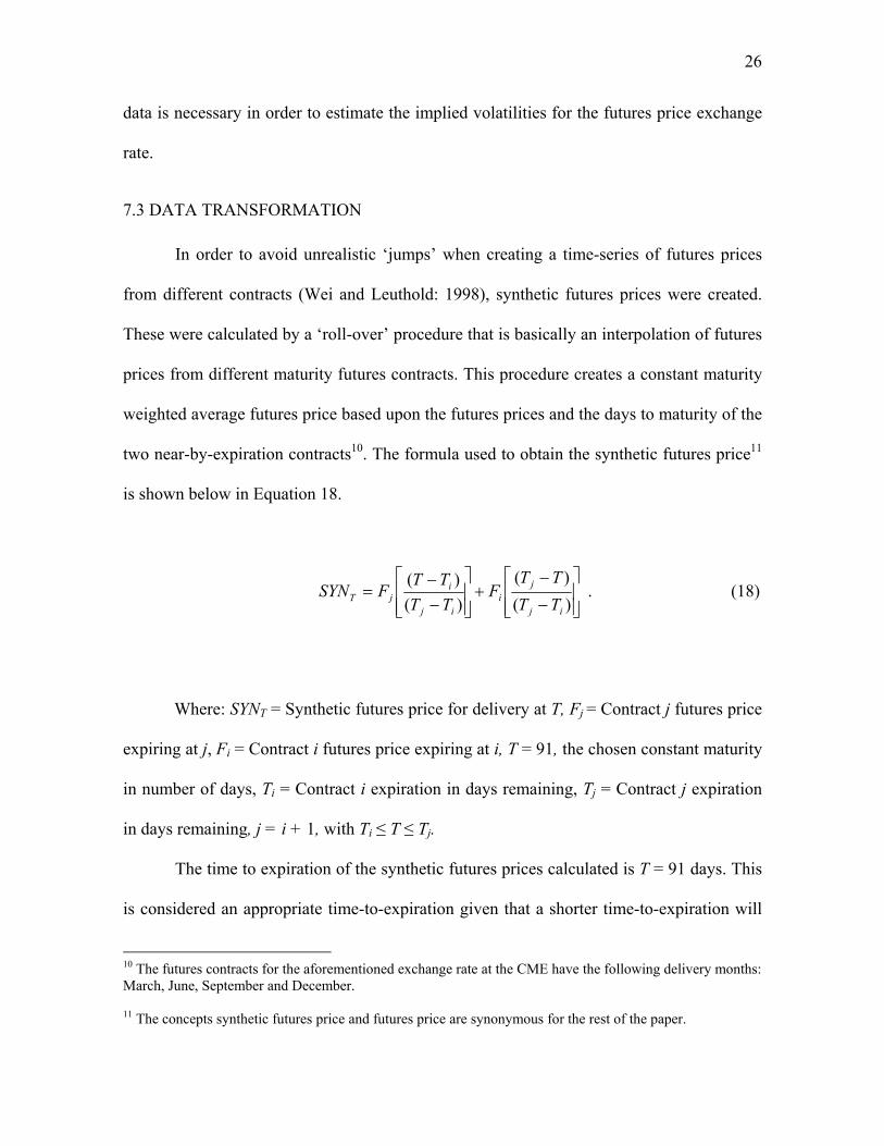
7.3 DATA TRANSFORMATION
In order to avoid unrealistic ‘jumps’ when creating a time-series of futures prices
from different contracts (Wei and Leuthold: 1998), synthetic futures prices were created.
These were calculated by a ‘roll-over’ procedure that is basically an interpolation of futures
prices from different maturity futures contracts. This procedure creates a constant maturity
weighted average futures price based upon the futures prices and the days to maturity of the
two near-by-expiration contracts10. The formula used to obtain the synthetic futures price11
is shown below in Equation 18.
⎥⎥⎦
⎤
⎢⎢⎣
⎡
−
−+
⎥⎥⎦
⎤
⎢⎢⎣
⎡
−−
=)()(
)()(
ij
ji
ij
ijT TT
TTF
TTTT
FSYN . (18)
Where: SYNT = Synthetic futures price for delivery at T, Fj = Contract j futures price
expiring at j, Fi = Contract i futures price expiring at i, T = 91, the chosen constant maturity
in number of days, Ti = Contract i expiration in days remaining, Tj = Contract j expiration
in days remaining, j = i + 1, with Ti ≤ T ≤ Tj.
The time to expiration of the synthetic futures prices calculated is T = 91 days. This
is considered an appropriate time-to-expiration given that a shorter time-to-expiration will
10 The futures contracts for the aforementioned exchange rate at the CME have the following delivery months: March, June, September and December. 11 The concepts synthetic futures price and futures price are synonymous for the rest of the paper.

27
give higher expected volatility. This situation is observed in empirical research papers,
which have found that volatility in futures prices increases, as a contract gets closer to
expiration (Samuelson: 1965). A higher expected volatility due to time-to-expiration could
have biased the results of this analysis. Thus, 91-day synthetic futures prices were
considered appropriate using this method in order to avoid high volatility estimates due to
time-to-expiration causes. In addition this will always allow finding a shorter and longer
contract, if necessary to do more analysis regarding time to maturity of the contracts.
VIII. DESCRIPTIVE STATISTICS
This subsection presents the descriptive statistics for the realised volatilities of the
exchange rate futures returns and the volatility forecasting models. The sample sizes for the
GARCH(1,1), the bi-variate and tri-variate BEKK(1,1) models are from 03/09/2001 to
05/01/2004. The sample sizes of the realised volatilities, the option implieds and the
composite forecast models are from 02/01/2002 to 05/01/2004. The sample sizes for the
historical models (conditional autoregressive models) are larger given that more data was
available for the author. Prior to fitting the ARCH models ARCH effects tests were
conducted on the series under analysis. This was done in order to see if the series had
ARCH effects therefore to make sure that these types of models are appropriate for the
data. The test conducted was the ARCH-LM test following the procedure of Engle (1982).
According to the results it was shown that all the series under study i.e. the spot, futures
prices and the interest rates had ARCH effects12. Under the null of homoscedasticity in the
12 These tests were conducted regressing the logarithmic returns of the series under analysis against a constant. The ARCH-LM test is the performed on the residuals of that regression. The test consists on regressing the square residuals against a constant and lagged values of the same square residuals. Five lags were applied on each test.

28
errors the F-statistics were 3.7620 for the spot, 7.6433 for the futures and 19.7698 for the
US interest rates. Therefore the null hypothesis was rejected in favour of heteroscedasticity
on those errors.
Figure 1 presents the natural logarithms (logs) of the spot and futures prices in
terms of Mexican pesos per USD and the realised volatility of the synthetic futures price.
The realised volatility graph is truncated at 0.002. Two observations are not observed in the
graph which are for the days 13/03/2003 – 14/03/2003 were it was observed higher than
usual volatility.
Table 1 show the descriptive statistics for the realised volatility and the forecasting
models. As it can be observed in Table 1 the means of the option implied and the variances
of the realised volatilities are the ones with higher values. These findings are consistent
with Christensen and Prabhala (1998) who found that the means of the option implieds
were higher than the means of the realised volatilities and that the variances of the realised
volatilities were higher than the variances of the option implieds. The distributions in that
table are highly skewed and leptokurtic indicating non-normality of the returns and the
forecast estimates. This is consistent with the work of Wei and Leuthold (1998) who
analysed volatility in futures markets and had similar findings with daily futures price
volatility.
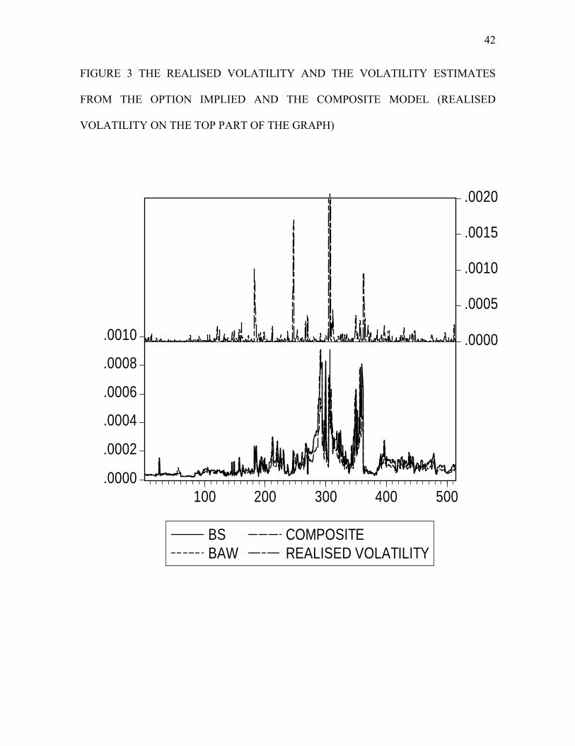
Lastly, Figures 2 and 3 presents the observations of the realised volatility (top line)
and the estimates of the historical models, the option implieds and the composite forecast
model. Again, the realised volatility graph is truncated at 0.002. It can be observed that in
both graphs all of the models capture the high volatility periods shown with the realised
volatility. At simple sight the implied volatility models estimates are almost the same.

29
IX. RESULTS
9.1 IN-SAMPLE EVALUATION
The OLS estimates for the weights of the composite forecast model (Equation 14
above) and the results of the MSE are presented in Tables 2 - 3. In Table 2 the third row
presents the estimates of the regression of the realised volatility against the historical
TVBEKK(1,1) model. The fourth row presents the estimates of the regression of the
realised volatility against the BS implied volatility model. The last column presents the
estimates of the regression of the realised volatility against both of the models. The weights
are taken from the last row. The TVBEKK and BS models were chosen given that they had
superior forecast accuracy in terms of MSE. As it can be observed in Table 2 the OLS
estimates show that the implied volatilities contain more of the information content of the
realised volatility for the returns when they are compared with the other forecast models.
However, it is difficult to find conclusive answers about their statistical power because the
adjusted R2 are remarkably low i.e. 0.0599.
In Table 3 it can be observed that the most accurate model is the composite forecast
model given that it has the lowest MSE. These results are consistent with Kroner et. al.
(1994), Blair, Poon and Taylor (2001) and Manfredo13 et. al. (2001), Fang (2002) who
found the most accurate volatility forecasts using composite forecast models. The second
best returns volatilities forecasts are the implied volatility models not being combined.
These results are consistent to that part of the literature who argues in favour of option
implied volatility in terms of forecasting accuracy. The differences of the MSE among the
models in Table 3 are statistically significant at the 1% level. The p-values rejected the null
13 In Manfredo et. al. (2001) the forecast time horizon was a one-week volatility forecast for the case of corn.

30
hypothesis of equality of forecast accuracy at that level. The null hypothesis is the
composite forecast against each of the remaining models. By rejecting the null it means that
there is statistical significant difference between the forecasts of the two models evaluated.
The procedure applied to obtain these statistical significances is the same as the one
described in Diebold and Mariano (1995)14.
9.2 OUT-OF-THE-SAMPLE EVALUATION
The sample period under analysis is partitioned in order to evaluate the out-of-the-
sample forecasts. The estimates (in-sample) for all the models are obtained from 2nd
January 2002 to 30th December 2002 for a total of 256 observations (about half the total
number of observations). The jump-off period is 31st December 2002, thus the out-of-the-
sample evaluation for all the forecasting models is from 31st December 2002 to 5th January
2004. The estimates (weights) of the OLS regressions (Equation 14 above) and the out-of-
the-sample results of the MSE can be observed in Table 4 - 5 respectively.
The variables chosen for the composite model were the ones with superior forecast
accuracy (lowest MSE) in the in-sample evaluation. These were the tri-variate ARCH for
the historical and the Black-Scholes for the option implied. The results of the estimates for
each variable alone in addition to the composite weights are presented in Table 4.
14 This method requires generating a time series, which is the differential of the squared-forecast errors from
two different forecast models i.e. ( ) ( )21,222
1,12 ˆˆ −− −−−= tttttd σσσσ , where dt is the differential of the
series and iσ̂ is the forecast of the i model. The t-statistic is obtained in the following way,
nsd
dwhere
d is the sample mean and sd is equal to the standard deviation of the series. The other variables are the same as described previously.

31
According to these estimated parameters in Table 4, it is possible to observe that the option
implied contains more information of the realised volatility compared to the historical
volatility model (TVBEKK). The out-of-the-sample evaluation shows that the results are
qualitatively similar to the in-sample evaluation (Table 3) although not the same. The
composite forecast models were the most accurate models in the in-sample evaluation.
However it was shown that within the composite specification the option implied is the best
model in terms of the relevant information about the realised volatility i.e. out performing
the TVBEKK(1,1) model15. That was consistent in both evaluation procedures: the in-
sample and the out-of-the-sample. It can be observed in Table 5 that for the out-of-the-
sample evaluation the option implied models have the lowest MSE thus, they were the most
accurate models for forecasting futures returns of the exchange rate under analysis. The
second in superiority was the composite model performing with more accuracy if compared
with the historical models. The MSE differences in this table are statistically significant at
the 5% level. The null hypothesis is the option implied models against each of the
remaining models.
X. CONCLUSION
The on-going debate related to which is the most accurate model to forecast
volatility of price returns of financial assets has led academic researchers to foster empirical
research on the aforementioned topic. A considerable amount of research projects have
compared time-series models against option implied volatilities and for instance composite
forecast models. The objective is to find the most accurate model (historical, option implied
15 Additional specifications in the composite model were also tried. The results were qualitatively similar showing more information content from options than from historical models (GARCH, BVBEEK).

32
or combined) to forecast price return volatility for specific assets. Albeit part of the
literature advocates the use of option implied volatilities as the most accurate alternative to
forecast price returns volatilities there are still no conclusive answers in terms of finding
one superior model. This is because the coefficients of determination are usually relatively
low for all models.
In this paper the aforementioned volatility forecast models i.e. time-series, option
implied and composite forecast models were compared to each other in order to find the
most accurate volatility forecasting model for the futures price returns of the Mexican peso
– US Dollar exchange rate. According to the results the implied volatilities contained most
of the information content of the realised return volatility for that exchange rate time series.
Similar findings can be found in the academic literature for agricultural commodities, stock
prices and stock indexes. The results also show that the composite forecast model was the
most accurate model in an in-sample evaluation when they were compared to the
alternative models not being combined. For the out-of-the-sample evaluation the implied
volatility forecasts proved to be superior to the other models. In terms of in-sample
evaluation, these findings are consistent with part of the academic literature, which states
that composite approaches are the most accurate alternative to forecast price returns
volatilities. However, these results should be taking with caution given the low statistical
power of the regressions (low coefficients of determination). Nonetheless, it is
recommended that in order to have the most accurate volatility forecast both type of data
i.e. historical and option implied should be used within a composite forecast framework.
Especially if both type of data are available.

33
BIBLIOGRAPHY
Akgiray, V. (1989). Conditional Heteroscedasticity in Time Series of Stock Returns: Evidence and Forecasts. Journal of Business. Vol. 62. (55-80).
Baba, Y., Engle, R. F., Kroner, K. F. and Kraft, D. (1992). Multivariate Simultaneous Generalized ARCH. Economics Working Paper 92 – 5. University of Arizona, Tucson.
Barone-Adesi, G. and Whaley, R. E. (1987). Efficient Approximation of American Option Values. The Journal of Finance. Vol. 42. June. (301-320).
Bates, J. M. and Granger, C. W. J. (1969) The Combination of Forecasts. Operations Research Quarterly. Vol. 20. (451 – 468).
Benavides, G. (2003). Price Volatility Forecasts for Agricultural Commodities: An Application of Historical Volatility Models, Option Implieds and Composite Approaches for Futures Prices of Corn and Wheat. Workingpaper.
Berndtand, E. Hall, B. Hall, R. and Hausman, J. (1974). Estimation and Inference in Nonlinear Structural Models. Annals of Economic and Social Measurement. (653-665).
Bessler, D. A. and Brandy, J. A. (1981) Forecasting Livestock Prices with Individual and Composite Methods. Applied Economics. Vol. 13. (513 – 522).
Black, F. and Scholes, M. S. (1973) The Pricing of Options and Corporate Liabilities. Journal of Political Economy. Vol. 81. May-June (637 – 654).
34
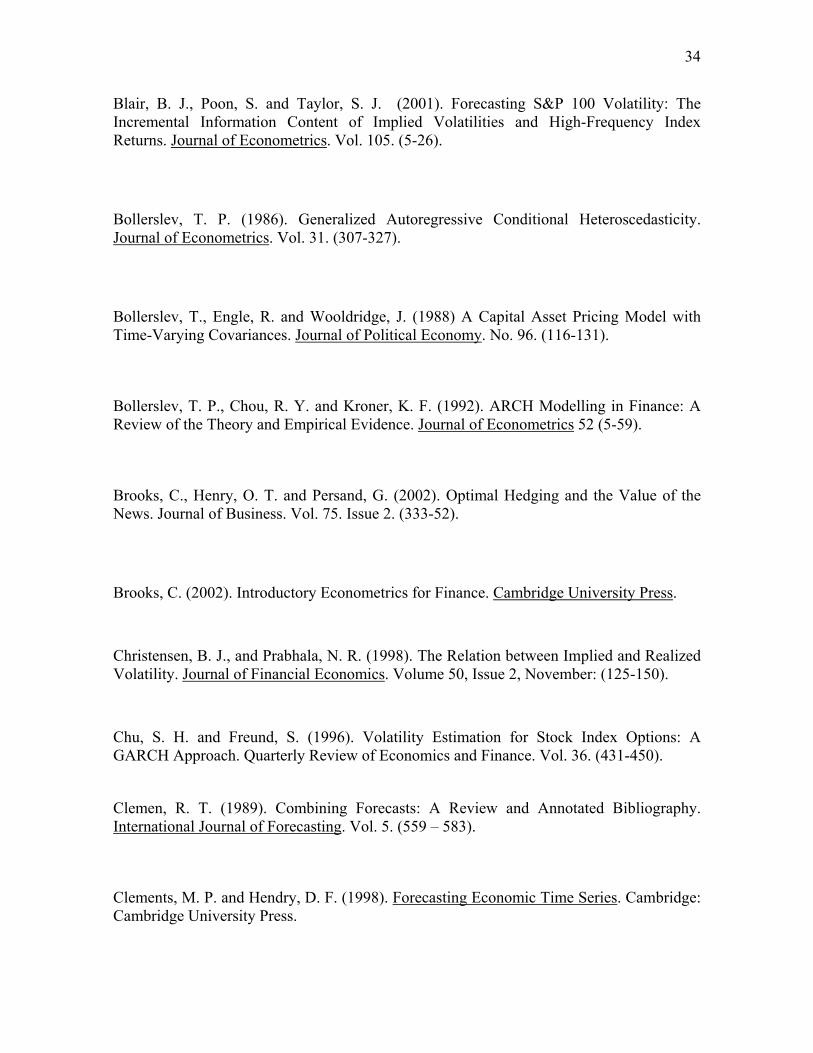
Blair, B. J., Poon, S. and Taylor, S. J. (2001). Forecasting S&P 100 Volatility: The Incremental Information Content of Implied Volatilities and High-Frequency Index Returns. Journal of Econometrics. Vol. 105. (5-26).
Bollerslev, T. P. (1986). Generalized Autoregressive Conditional Heteroscedasticity. Journal of Econometrics. Vol. 31. (307-327).
Bollerslev, T., Engle, R. and Wooldridge, J. (1988) A Capital Asset Pricing Model with Time-Varying Covariances. Journal of Political Economy. No. 96. (116-131).
Bollerslev, T. P., Chou, R. Y. and Kroner, K. F. (1992). ARCH Modelling in Finance: A Review of the Theory and Empirical Evidence. Journal of Econometrics 52 (5-59).
Brooks, C., Henry, O. T. and Persand, G. (2002). Optimal Hedging and the Value of the News. Journal of Business. Vol. 75. Issue 2. (333-52).
Brooks, C. (2002). Introductory Econometrics for Finance. Cambridge University Press.
Christensen, B. J., and Prabhala, N. R. (1998). The Relation between Implied and Realized Volatility. Journal of Financial Economics. Volume 50, Issue 2, November: (125-150).
Chu, S. H. and Freund, S. (1996). Volatility Estimation for Stock Index Options: A GARCH Approach. Quarterly Review of Economics and Finance. Vol. 36. (431-450).
Clemen, R. T. (1989). Combining Forecasts: A Review and Annotated Bibliography. International Journal of Forecasting. Vol. 5. (559 – 583).
Clements, M. P. and Hendry, D. F. (1998). Forecasting Economic Time Series. Cambridge: Cambridge University Press.

35
Day, T. E. and Lewis, C. M. (1992). Stock Market Volatility and the Information Content of Stock Index Options. Journal of Econometrics. Vol. 52. (267-287).
Diebold, F. X. and Mariano, R. S. (1995). Comparing Predictive Accuracy. Journal of Business and Economic Statistics. Vol. 13. (253-263).
Ederington, L. and Guan, W. (2002), Is implied Volatility an Informationally Efficient and Effective Predictor of Future Volatility? Journal of Risk. Vol. 4 (3). Engle, R. F. (1982) “Autoregressive Conditional Heteroskedasticity with Estimates of the Variance of U.K. Inflation,” Econometrica, 50, (987–1008).
Engle, R. F. (2000). Dynamic Conditional Correlation – A Simple Class of Multivariate GARCH Models. SSRN Discussion Paper 2000-09. University of California, San Diego. May 2000.
Engle, R. F. and Kroner, K. (1995). Multivariate Simultaneous Generalized ARCH. Econometric Theory 11. (122-150).
Fang, Y. (2002) Forecasting Combination and Encompassing Tests. International Journal of Forecasting. Vol. 1. Elsevier Science B. V. Figlewski, S. (1997). Forecasting Volatility. Financial Markets, Institutions, and Instruments. Vol. 6. (2-87).
Fleming, J. (1998). The Quality of Market Volatility Forecasts Implied by S & P 100 Index Option Prices. Journal of Empirical Finance. Vol. 5. (317-345). Giot, P. (2003). Implied Volatility Indexes and Daily Value-at-Risk Models. Workingpaper. Department of Business Administration & CEREFIM at University of Namur, Belgium.

36
Granger, C. W. J. and Ramanathan, R. (1984). Improved Methods of Combining Forecasts. Journal of Forecasting. Vol. 3. (197-204).
Haigh, M. S. and Holt, M. T. (2000). Hedging Multiple Price Uncertainty in International Agricultural Trade. American Journal of Agricultural Economics. Vol. 82 No. 4 November. (881-896).
Harvey, C. R. and Whaley, R. E. (1992). Dividends and S&P 100 Index Options. Journal of Futures Markets. Vol. 12. (123 – 137). Hull, J. 2003. Options, Futures and Other Derivatives. 5th. Edition. Prentice Hall.
Jorion, P. (1995). Predicting Volatility in the Foreign Exchange Market. The Journal of Finance. Vol. 50 (507-528). Kroner, K., Kneafsey, K. P. and Claessens, S. (1994). Forecasting Volatility in Commodity Markets. Journal of Forecasting. Vol. 14. (77-95).
Lamoureux, C. G. and Lastrapes, W. D. (1993). Forecasting Stock Return Variance: Toward an Understanding of Stochastic Implied Volatilities. The Review of Financial Studies. Vol. 6. (293-326).
Levich R. M. 1998. International Financial Markets: Prices and Policies. Boston, Mass.:
Irwin McGraw-Hill.
Makridakis, S. (1989). Why Combining Works? International Journal of Forecasting. Vol. 5. (601-603).
Manfredo, M. Leuthold, R. M. and Irwin, S. H. (2001). Forecasting Cash Price Volatility of Fed Cattle, Feeder Cattle and Corn: Time Series, Implied Volatility and Composite Approaches. Journal of Agricultural and Applied Economics. Vol. 33. Issue 3 December. (523-538).

37
Martens, M., and Zein, J. (2002). Predicting Financial Volatility: High-Frequency Time-Series Forecasts vis-à-vis Implied Volatility, Mimeo, Erasmus University Rotterdam. Neely, C.J., (2002). Forecasting Foreign Exchange Volatility: Is implied Volatility the Best We Can Do? Federal Reserve Bank of St. Louis, Workingpaper 2002-017. Ng, V. K and Pirrong, S. C. 1994. Fundamentals and Volatility: Storage, Spreads, and the Dynamic of Metals Prices. Journal of Business 67 (203-230). Park, D. W. and Tomek, W. G. (1989). An Appraisal of Composite Forecasting Methods. North Central Journal of Agricultural Economics. Vol. 10. (1-11).
Pojarliev, M. and Polasek, W. (2000). Portfolio Construction by Volatility Forecasts: Does the Covariance Structure Matter? Financial Markets and Portfolio Management, 2003, 17 (1), pages 103-117. Poon, S-H. and Granger, C. (2003). Forecasting Volatility in Financial Markets: A Review, Forthcoming in the Journal of Economic Literature. Pong, S., Shackleton, M., Taylor, S. and Xu, X. (2003) Forecasting Currency Volatility: A Comparison of Implied Volatilities and AR(FI)MA models. Forthcoming, Journal of Banking and Finance. Ng, V. K and Pirrong, S. C. (1994). Fundamentals and Volatility: Storage, Spreads, and the Dynamic of Metals Prices. Journal of Business 67 (203-230). Samuelson, P. (1965). Proof that Properly Anticipated Prices Fluctuate Randomly. Industrial Management Review, 6 Spring: (41-49). Schroeder, T. C., Albright, M. L., Langemeier, M. R. and Mintert, J. (1993). Factors Affecting Cattle Feeding Profitability. Journal of the American Society of Farm Managers and Rural Appraisers. 57: (48-54). Susmel, R. and Thompson, R. (1997). Volatility, Storage and Convenience Evidence from Natural Gas Markets Journal of Futures Markets Vol. 17. No. 1 (17-43).

38
Taylor, S. J. (1985). The Behaviour of Futures Prices Overtime. Applied Economics, 17:4 Aug: (713-734). Wei, A. and Leuthold, R. M. (1998). Long Agricultural Futures Prices: ARCH, Long Memory, or Chaos Processes. OFOR Paper Number 98-03. Xu, X. and Taylor, S. J. 1995. Conditional Volatility and the Informational Efficiency of the PHLX Currency Options Market. Journal of Banking and Finance. Vol. 19, (803-821).

39
APPENDIX
FIGURE 1 THE REALISED VOLATILITY OF THE FUTURES PRICE AND THE
NATURAL LOGARITHM OF THE SPOT AND FUTURES PRICES OF THE
EXCHANGE RATE PESO – USD (REALISED VOLATILITY ON THE TOP PART OF
THE GRAPH)
2.1
2.2
2.3
2.4
2.5 .0000
.0005
.0010
.0015
.0020
100 200 300 400 500
LOG SPOT PRICELOG FUTURES PRICEREALISED VOLATILITY

40
TABLE 1 DESCRIPTIVE STATISTICS FOR THE REALISED VOLATILITY AND THE
VOLATILITY FORECASTING MODELS OF THE DAILY FUTURES PRICE
RETURNS OF THE MEXICAN PESO-USD EXCHANGE RATE
Model Mean Variance Skewness Kurtosis N
Realised volatility
6.40 x 10⁻⁵ 1.52 x 10⁻⁷ 17.7230 356.6332 513
GARCH(1,1) 6.75 x 10⁻⁵ 1.70 x 10⁻⁸ 11.1848 156.0621 595
Bi-variate BEKK(1,1)
7.43 x 10⁻⁵ 2.3 x 10⁻⁸ 10.6991 142.4607 595
Tri-variate BEKK(1,1)
6.83 x 10⁻⁵ 1.4 x 10⁻⁸ 9.8068 119.1293 595
BS option implied
0.000125 1.7 x 10⁻⁸ 3.0657 14.4143 513
BAW option implied
0.000125 1.7 x 10⁻⁸ 3.0663 14.4187 513
Composite forecast
9.68 x 10⁻⁵ 9.0 x 10⁻⁹ 3.5656 20.3474 513
This table reports the descriptive statistics of the realised volatility and the volatility
forecasting models for the daily futures prices returns of the Mexican peso-USD exchange
rate. The daily BS option implied volatility is computed using the Black-Scholes model
(1973) and the BAW option implied volatility is calculated using an approximating
American option price formula as described in Barone-Adesi and Whaley (1987). The
options data are call options at-the-money (or the closest to at-the-money) with at least
fifteen days prior to expiration. The realised volatility used to obtain the composite forecast
model is the annualised ex-post daily futures return volatility for the respective sample
period under analysis. The sample size for the GARCH(1,1), the bi-variate and tri-variate
BEKK(1,1) models is 597 observations (two observations are lost because of the lags in the
models) from 3rd September 2001 to 5th January 2004. The sample size for the realised
volatility, the option implied and the composite models is 513 observations from 2nd
January 2002 to 5th January 2004. N = Number of observations.

41
FIGURE 2 THE REALISED VOLATILITY AND THE VOLATILITY ESTIMATES
FROM THE HISTORICAL MODELS (REALISED VOLATILITY ON THE TOP PART
OF THE GRAPH)
.0000
.0005
.0010
.0015
.0020
.0025
.0030.0000
.0005
.0010
.0015
.0020
100 200 300 400 500
GARCHBVBEKK
TVBEKKREALISED VOLATILITY
42
FIGURE 3 THE REALISED VOLATILITY AND THE VOLATILITY ESTIMATES
FROM THE OPTION IMPLIED AND THE COMPOSITE MODEL (REALISED
VOLATILITY ON THE TOP PART OF THE GRAPH)
.0000
.0002
.0004
.0006
.0008
.0010 .0000
.0005
.0010
.0015
.0020
100 200 300 400 500
BSBAW
COMPOSITEREALISED VOLATILITY

43
TABLE 2 IN-SAMPLE OLS ESTIMATES FOR WEIGHTS IN THE COMPOSITE
MODEL
INDEPENDENT VARIABLES ADJ. R2 DW
INTERCEPT TVBEKK(1,1) BS OPTION
IMPLIED
3.35 x 10⁻⁵ (1.96 x 10-5)* 1.7075
0.4278 (0.1357)** 3.1522
N.A. 0.0191 2.1576
-2.14 x 10⁻⁵ (2.32 x 10⁻⁵) -0.9225
N.A. 0.6814 (0.1277)** 5.3343
0.0528 1.9677
-3.28 x 10⁻⁵ (2.38 x 10⁻⁵) -1.3746
0.2706 (0.1371)** 1.9732
0.6183 (0.1314)** 4.7077
0.0599 2.1136
This table presents estimates of OLS regressions of the variables in the second row
(independent variables) against the realised volatility of the exchange rate. Third row
presents the estimates of the regression of the realised volatility against the historical
TVBEKK(1,1) model. Fourth row presents the estimates of the regression of the realised
volatility against the BS implied volatility model. The last column presents the estimates of
the regression of the realised volatility against both of the models. The weights are taken
from the last row. Standard errors are shown in brackets. Italics = t-statistic. (**) Indicates
the coefficient is statistically significant at the 5% confidence level; (*) indicates the
coefficient is statistically significant at the 10% confidence level. Adj. R2 = Adjusted
coefficient of determination. DW = Durbin Watson statistic. The sample size for the
estimates of the regressions is 513 observations from 2nd January 2002 to 5th January 2004.
N.A = Not applicable.

44
TABLE 3 IN-SAMPLE MSE FOR THE EXCHANGE RATE FORECASTS
FORECAST
MODEL
MSE P-VALUE RANK
GARCH(1,1) 1.57586 x 10⁻⁷ 0.00205 5
BVBEKK(1,1) 1.61497 x 10⁻⁷ 0.00015 6
TVBEKK(1,1) 1.5466 x 10⁻⁷ 0.00055 4
BS option implied 1.49786 x 10⁻⁷ 0.00046 2
BAW option implied
1.49788 x 10⁻⁷ 0.00187 3
Composite model 1.44023 x 10⁻⁷* N.A 1
This table reports MSE of the volatility forecasting models for the daily futures
prices returns for the Mexican peso-USD exchange rate. The daily option implied volatility
is computed using the Black-Scholes (1973) model and an approximating American option
price formula as described in Barone-Adesi and Whaley (1987). The options data are call
options at-the-money (or the closest to at-the-money) with at least fifteen days prior to
expiration. The realised volatility used to obtain the MSE is the annualised ex-post daily
futures return volatility for the sample period under analysis. P-Values are referred to the
procedure to obtain statistical significances in MSE for each model against the composite
model according to Diebold and Mariano (1995). Rank 1 = Highest, 6 = lowest. The sample
size for the GARCH(1,1) and the BEKK(1,1) models is 597 observations from 3rd
September 2001 to 5th January 2004. The sample size for the implied and the composite
models is 513 observations from 2nd January 2002 to 5th January 2004. The sample size to
calculate the MSE is the same as for the implied and the composite models i.e. 513
observations from 2nd January 2002 to 5th January 2004. (*) Indicates the smallest value.
N.A = Not applicable.

45
TABLE 4 IN-SAMPLE OLS ESTIMATES FOR THE OUT-OF-THE SAMPLE
EVALUATION OF THE EXCHANGE RATE VOLATILITY PESO-USD
INDEPENDENT VARIABLES ADJ. R2 DW
INTERCEPT TVBEKK(1,1) BS OPTION
IMPLIED
4.87 x 10⁻⁷ (1.38 x 10⁻⁵) -0.0353
0.7408 (0.1601)** 4.6263
N.A. 0.0777 1.2801
-1.36 x 10⁻⁵ (1.69 x 10⁻⁵) -0.8049
N.A. 0.8655 (0.2008)** 4.3087
0.0681 1.0284
4.50 x 10⁻⁵ (1.80 x 10⁻⁵)** -2.4930
0.6526 (0.1578)** 4.1348
0.7452 (0.1969)** 3.7834
0.1271 1.2419
This table presents estimates of OLS regressions of the variables in the second row
(independent variables) against the realised volatility of the respective commodity
(dependent variable). Standard errors are shown in brackets. Italics = t-statistic. (**)
Indicates the coefficient is statistically significant at the 5% confidence level; (*) indicates
the coefficient is statistically significant at the 10% confidence level. Adj. R2 = Adjusted
coefficient of determination. DW = Durbin Watson statistic. The sample size for the
BEKK(1,1) model is 5,297 observations from 2nd January 1975 to 3rd January 1996. The
sample size for the implied and the composite models is 757 observations from 2nd January
1993 to 3rd January 1996. N.A = Not applicable.

46
TABLE 5 OUT-OF-THE-SAMPLE MSE FOR THE EXCHANGE RATE FORECASTS
FORECAST
MODEL
MSE P-VALUE RANK
GARCH(1,1) 2.84 x 10⁻⁷ 0.0004 6
BVBEKK(1,1) 2.77 x 10⁻⁷ 0.0003 5
TVBEKK(1,1) 2.76 x 10⁻⁷ 0.0002 4
BS option implied 2.65 x 10⁻⁷* N.A 1
BAW option implied
2.65 x 10⁻⁷* N.A 1
Composite model 2.69 x 10⁻⁷ 0.0001 3
This table reports the out-of-the-sample MSE of the volatility forecasting models
for the daily futures prices returns of the exchange rate Mexican peso - USD. The daily
option implied volatility is computed using the Black-Scholes (1973) model and an
approximating American option price formula as described in Barone-Adesi and Whaley
(1987). The options data are call options at-the-money (or the closest to at-the-money) with
at least fifteen days prior to expiration. The realised volatility used to obtain the MSE is the
annualised ex-post daily futures return volatility for the sample period under analysis. Rank
1 = Highest, 6 = lowest. The in-sample size for all the models is 256 observations (about
half the total number of observations) from 2nd January 2002 to 30th December 2002. The
out-of-the-sample forecast evaluation period consists of 257 observations from 31st
December 2002 to 5th January 2004. The jump-off period is 31st December 2002. (*)
Indicates the smallest value. N.A = Not applicable.