Embed Size (px)
Citation preview

PREDICTIVE MODELING FOR INTELLIGENT MAINTENANCE IN COMPLEX SEMICONDUCTOR MANUFACTURING PROCESSES
by
Yang Liu
A dissertation submitted in partial fulfillment of the requirements for the degree of
Doctor of Philosophy (Mechanical Engineering)
in The University of Michigan 2008
Doctoral Committee:
Professor Jun Ni, Chair Associate Professor Jionghua Jin Assistant Professor Amy E. Cohn Assistant Professor Kathleen H. Sienko

Copyright © 2008 by Yang Liu
All Rights Reserved

ii
For my beloved wife Min

iii
ACKNOWLEDGEMENTS
I would like to take this opportunity to express my heartfelt gratitude to a number
of people without whose help and support this thesis would never have been finished.
First of all, I must start with my respectable advisor Professor Jun Ni for his wise
supervision, guidance, and encouragement. Without his continuous support, this thesis
would have not been accomplished. Professor Ni gave me a lot of innovative ideas and
constructive comments in all the time of my research. I will always be grateful for the
great opportunities he has extended to me during my PhD study in S. M. Wu
Manufacturing Research Center.
I am deeply grateful to Dr. Dragan Djurdjanovic, who has always worked closely
with me, spent his valuable time to look into every detail of my results, and given
invaluable advices. Dr. Dragan Djurdjanovic has taught me on writing papers and
presenting results effectively, which in turn helped me to earn two Best Paper awards.
I would like to acknowledge my appreciation to Professor Jionghua Jin, Professor
Amy Cohn, and Professor Kathleen Sienko for taking their valuable time to be on my
committee, reading my thesis and offering insightful suggestions. In addition, I would
like to thank Professor Kathleen Sienko for the support and advices when I was assisting
her teaching Dynamics & Vibration course.

iv
I would like to express my thankfulness to Professor Karl Grosh, Professor
Richard Scott, Professor Yavuz Bozer, Professor Jianjun Shi, and Professor Michael
Chen for their interesting lectures and generous help during my study in Michigan.
Special thank goes to Professor Karl Grosh who has extended me great opportunities to
be a teaching assistant in the most competitive environment.
I would like to thank Kathleen Hoskins, Sarah Packard, Lin Li, Adam Brzezinski,
Seungchul Lee, Li Jiang, Masahiro Fujiki, Kwanghyun Park, and all members of S. M.
Wu Manufacturing Research Center for their assistances. I would like to thank my friends
Xi Charles Zhang, Weifeng Ye, Hui Li, Rui He, Jiang Wang, Honghai Zhu, Jing Zhou,
Zhen Zhang, Yong Lei, Rui Li, Jianbo Liu, Jaspreet Dhupia, Ran Jin, and Zhenhua
Huang for their kindest help during the past three years.
Last but by no means least I would like to thank my parents and parents-in-law
for their countless love and support. Finally, I would like to dedicate this work to my wife
who has been my best friend and source of strength for more than eleven years, and
without her encouragement and support this thesis would never have started, much less
finished.

v
TABLE OF CONTENTS
DEDICATION................................................................................................................... ii
ACKNOWLEDGEMENTS ............................................................................................ iii
LIST OF TABLES .......................................................................................................... vii
LIST OF FIGURES ......................................................................................................... ix
LIST OF ACRONYMS .................................................................................................. xii
ABSTRACT ................................................................................................................... xiv
CHAPTER 1 INTRODUCTION................................................................................1
1.1. Motivation ..........................................................................................................1
1.2. Research Objectives ...........................................................................................3
1.3. Organization of Dissertation ..............................................................................6
CHAPTER 2 LITERATURE REVIEW ...................................................................8
2.1. Introduction ........................................................................................................8
2.2. OSA-CBM Standard ........................................................................................11
2.3. Predictive Maintenance in Semiconductor Manufacturing ..............................13
2.4. Potential Research Directions ..........................................................................27
CHAPTER 3 PREDICTIVE MODELING OF MULTIVARIATE STOCHASTIC DEPENDENCIES USING BAYESIAN NETWORK ........................................................................................30

vi
3.1. Introduction ......................................................................................................30
3.2. Relevant Modeling Components ......................................................................32
3.3. Methodology Overview ...................................................................................38
3.4. Simulation Study ..............................................................................................41
3.5. Case Study I .....................................................................................................58
3.6. Case Study II ....................................................................................................70
3.7. Improvement of the Efficiency of Data Search ...............................................80
3.8. Conclusions ......................................................................................................82
CHAPTER 4 HIDDEN MARKOV MODEL BASED PREDICTION OF TOOL DEGRADATION UNDER VARIABLE OPERATING CONDITIONS...........................................................84
4.1. Introduction ......................................................................................................84
4.2. Hidden Markov Model Background ................................................................87
4.3. Proposed Method .............................................................................................90
4.4. Simulation Study ..............................................................................................94
4.5. Case Study .....................................................................................................110
4.6. Conclusions ....................................................................................................115
CHAPTER 5 IMPROVED MAINTENANCE DECISION USING PREDICTED PROCESS CONDITION AND PRODUCT QUALITY INFORMATION ..........................................................117
5.1. Introduction ....................................................................................................117
5.2. Proposed Method ...........................................................................................120
5.3. Case Study .....................................................................................................126
5.4. Conclusions ....................................................................................................132
CHAPTER 6 CONCLUSIONS AND FUTURE WORK .....................................133
6.1. Conclusions ....................................................................................................133
6.2. Original Contributions ...................................................................................135
6.3. Future Work ...................................................................................................137
BIBLIOGRAPHY ..........................................................................................................139

vii
LIST OF TABLES
Table 2.1 Category of maintenance strategies .................................................................... 8
Table 2.2 Sensor categories in semiconductor fabs .......................................................... 15
Table 3.1 Sixteen cases for A and B feature vectors .................................................. 44
Table 3.2 Inspection parameter combinations .................................................................. 44
Table 3.3 Predefined conditional probability P(C|A,B) .................................................... 45
Table 3.4 Predefined conditional probability for 1B and 2B given 1A and 2A ........ 46
Table 3.5 1B and 2B combinations .............................................................................. 46
Table 3.6 Relationship between 1A & 2A and labels (states) in Figure 3.5(b) .............. 48
Table 3.7 Relationship between 1B & 2B and labels (states) in Figure 3.6(b) ............ 48
Table 3.8 Relationship between 1P & 2P and labels (states) in Figure 3.7(b) ............. 49
Table 3.9 Tabulated probability distributions for P(A) and P(B) ..................................... 53
Table 3.10 Tabulated conditional probability P(C|A,B) from Bayesian learning ............ 55
Table 3.11 Tabulated conditional probability P(C|A,B) calculated from the model ........ 55
Table 3.12 Comparison of model probability and inference results (Example 1) ............ 57
Table 3.13 Comparison of model probability and inference results (Example 2) ............ 57
Table 3.14 Discretization results of process parameters ................................................... 64
Table 3.15 Conditional probability table for metrology node .......................................... 66
Table 3.16 Four-fold cross validation results ................................................................... 69
Table 3.17 Discretization results for 44 features on Part # 1 and Part # 2 ........................ 73

viii
Table 3.18 Similarity between inferred distributions and true distributions .................... 80
Table 3.19 Comparison between data search strategies .................................................... 82
Table 4.1 Emission probability table under single operating condition ........................... 99
Table 4.2 Emission probability table under variable operating conditions .................... 108
Table 5.1 Tool deterioration states and corresponding yields ........................................ 129
Table 5.2 Simulation parameters for improved maintenance policies ............................ 129
Table 5.3 Simulation results with different PdM policies .............................................. 130
Table 5.4 Comparison of maintenance cost for different policies .................................. 130

ix
LIST OF FIGURES
Figure 1.1 Illustration of research objectives ...................................................................... 5
Figure 2.1 OSA-CBM overview ....................................................................................... 12
Figure 2.2 Typical CMP metrologies and process control solutions ................................ 18
Figure 2.3 Performance evaluation using confidence value ............................................. 22
Figure 2.4 Overview of integrated APM system .............................................................. 27
Figure 3.1 Example of BNs used for modeling the direction of a car .............................. 36
Figure 3.2 Framework of multivariate stochastic dependencies modeling ....................... 39
Figure 3.3 Simulation scenario ......................................................................................... 42
Figure 3.4 Simulation flowchart ....................................................................................... 42
Figure 3.5 (a) Unified distance matrix for feature A ; (b) Labels for feature A ............ 47
Figure 3.6 (a) Unified distance matrix for feature B ; (b) Labels for feature B ............ 48
Figure 3.7 (a) Unified distance matrix for feature C ; (b) Labels for feature C ............ 49
Figure 3.8 Expected BN configuration after structure learning for two models: (a) A and B are independent; (b) B is dependent on A ......................................................... 50
Figure 3.9 BN configuration for A & B independent case: (a)-(c) different initial configurations; (d) final configuration after structure learning ............................ 51
Figure 3.10 BN configuration for A & B dependent case: (a)-(c) different initial configurations; (d) final configuration after structure learning ............................ 52
Figure 3.11 Probability inference examples in unit (%) ................................................... 56
Figure 3.12 Data consolidation and synchronization procedure ....................................... 59

x
Figure 3.13 Chamber tool process parameters .................................................................. 60
Figure 3.14 Zoom-in of PARAM4 to show the deviations embedded in the significant variation of mean values ....................................................................................... 61
Figure 3.15 Bayesian structure learning result ................................................................. 65
Figure 3.16 Example of probability inference .................................................................. 67
Figure 3.17 Comparison of true distribution to inferred distribution ............................... 68
Figure 3.18 Perceptron measurement of one feature variable .......................................... 71
Figure 3.19 Perceptron optical measurement features ...................................................... 71
Figure 3.20 Measurement features of Part # 1 and Part # 2 .............................................. 72
Figure 3.21 BN structure for 44 features on Part # 1 and Part # 2 (a) Labeled by feature names; (b) Labeled by feature numbers ................................................................ 75
Figure 3.22 BN Structures for (a) 24 features on Part # 1; (b) 20 features on Part # 2 .... 76
Figure 3.23 Inferred probability distributions for (a) feature # 8 and (b) feature # 11 ..... 78
Figure 3.24 True probability distributions for (a) feature # 8 and (b) feature # 11 .......... 79
Figure 3.25 Tree based organization of database using SOM Voronoi set tessellation ... 81
Figure 4.1 Graphical representation of the dependence structures of an HMM ............... 87
Figure 4.2 Framework of HMM based chamber degradation prediction ......................... 91
Figure 4.3 Illustration of modeling unobservable in-chamber degradation ...................... 93
Figure 4.4 Simulation flowchart ....................................................................................... 95
Figure 4.5 Exponential degradation curve under single operating condition ................... 96
Figure 4.6 Stochastic degradation process under single operating condition ................... 96
Figure 4.7 Stratified degradation states under single operating condition........................ 97
Figure 4.8 Illustration of 5-state unidirectional HMM ................................................... 100
Figure 4.9 Estimation of state transition (4-state HMM) ................................................ 102
Figure 4.10 Estimation of state transition (5-state HMM) .............................................. 104
Figure 4.11 Estimation of state transition (6-state HMM) .............................................. 105

xi
Figure 4.12 Degradation curve under variable operating conditions .............................. 106
Figure 4.13 Stochastic degradation process under variable operating conditions .......... 107
Figure 4.14 Stratified degradation state under variable operating conditions ................ 107
Figure 4.15 Estimation of state transition under variable operating conditions ............. 110
Figure 4.16 HMM learning curve. .................................................................................. 112
Figure 4.17 Chamber deterioration and maintenance ..................................................... 114
Figure 5.1 Methodology framework of improved maintenance decision-making ......... 121
Figure 5.2 Interaction between discrete-event simulation and optimization methods .... 124
Figure 5.3 Modified BN structure including ‘Tool State’ .............................................. 128

xii
LIST OF ACRONYMS
ABM Age (or usage) Based Maintenance
AE Acoustic Emission
AI Artificial Intelligence
APC Advanced Process Control
APM Automated Precision Manufacturing
BMU Best Matching Unit
BN Bayesian Network
CBM Condition Based Maintenance
CMP Chemical Mechanical Planarization
CPT Conditional Probability Table
CVD Chemical Vapor Deposition
DNC Dynamic Neural Controller
EM Expectation Maximization
EWMA Exponentially Weighted Moving Average
FTIR Fourier Transform Infrared
GA Genetic Algorithm
HMM Hidden Markov Model
MDP Markov Decision Process

xiii
MIMO Multiple-Input Multiple-Output
MIP Mixed Integer Programming
MLE Maximum Likelihood Estimation
MVFD Multivariate Fault Detection
MWST Maximum Weight Spanning Tree
OES Optical Emission Spectroscopy
OSA-CBM Open System Architecture for Condition Based Monitoring
PCC Predictor Corrector Control
PdM Predictive Maintenance
PM Preventive Maintenance
RM Reactive Maintenance
SOM Self Organizing Map
SPC Statistical Process Control
SSE Sum of Squared Error
WIP Work In Progress
XRD X-ray Diffraction

xiv
ABSTRACT
Semiconductor fabrication is one of the most complicated manufacturing
processes, in which the current prevailing maintenance practices are preventive
maintenance, using either time-based or wafer-based scheduling strategies, which may
lead to the tools being either “over-maintained” or “under-maintained”. In literature,
there rarely exists condition-based maintenance, which utilizes machine conditions to
schedule maintenance, and almost no truly predictive maintenance that assesses
remaining useful lives of machines and plans maintenance actions proactively.
The research presented in this thesis is aimed at developing predictive modeling
methods for intelligent maintenance in semiconductor manufacturing processes, using the
in-process tool performance as well as the product quality information. In order to
achieve an improved maintenance decision-making, a method for integrating data from
different domains to predict process yield is proposed. The self-organizing maps have
been utilized to discretize continuous data into discrete values, which will tremendously
reduce the computational cost of Bayesian network learning process that can discover the
stochastic dependences among process parameters and product quality. This method
enables one to make more proactive product quality prediction that is different from
traditional methods based on solely inspection results.

xv
Furthermore, a method of using observable process information to estimate
stratified tool degradation levels has been proposed. Single hidden Markov model
(HMM) has been employed to represent the tool degradation process under a single
recipe; and the concatenation of multiple HMMs can be used to model the tool
degradation under multiple recipes. To validate the proposed method, a simulation study
has been conducted, which shows that HMMs are able to model the stratified
unobservable degradation process under variable operating conditions. This method
enables one to estimate the condition of in-chamber particle contamination so that
maintenance actions can be initiated accordingly.
With these two novel methods, a methodological framework to perform better
maintenance in complex manufacturing processes is established. The simulation study
shows that the maintenance cost can be reduced by performing predictive maintenance
properly while highest possible yield is retained. This framework provides a possibility of
using abundant equipment monitoring data and product quality information to coordinate
maintenance actions in a complex manufacturing environment.

1
CHAPTER 1
INTRODUCTION
1.1. Motivation
Modern complex manufacturing processes are often characterized by a large
number of processing steps, long duration of processing time, dynamic interactions
among different tools, and complex interrelations between tool performances and product
qualities. The semiconductor manufacturing is one of the examples of such processes,
which usually involves hundreds of processing steps, months of processing time, re-
entrant process flows, and unpredictable relationships between tools performances and
yield [1, 2].
Semiconductor manufacturers are facing increasingly competitive market
environment. Improving microchip productivity has always been a priority. New
microchips need to reach the market in adequate quantity, quality and reasonable price in
order to attain and maintain the market share. In addition, with the use of 300mm wafer
production, automation level in the fabrication facility (fab) also increased with a larger
number of in-situ sensors embedded in the equipment. Furthermore, since the majority of
the equipment is relatively new, there is not much established historical reliability data.
Moreover, high mix and low volume production demands require tighter controls on

2
reducing the downtime and increasing the yield. Therefore, wafer fabrication facilities all
around the world have been looking into methods and techniques to:
1) Increase the wafer yield so that more qualified products can be shipped out;
2) Achieve near-zero-downtime in the fabrication system so that all machines in
the fab are spending more of their life creating values rather than idling;
3) Realize shorter cycle time.
However, several existing issues set barriers to accomplish these goals:
• Fragmented data and information domains with limited information sharing
between inspection, maintenance and process control operations;
• Limited and unreliable in-chamber contamination monitoring information;
• Limited or non-existent linkage of equipment/station specific information with
that corresponding to preceding and succeeding equipment;
• Limited amount of historical reliability data on equipment due to frequent
introduction of new equipment and changes in process parameter settings.
Currently, the majority of maintenance operations in the semiconductor industry
are still based on either historical reliability of fabrication equipment, or on diagnostic
information from equipment performance signatures extracted from in-situ sensors. Such
a fragmented, “diagnosis-centered” approach leads to mostly preventive maintenance
along with reactive maintenance policies that use neither abundant product quality,
equipment condition, equipment reliability information, nor the temporal dynamics inside
that information in order to anticipate future events in the system and thus facilitate a
more proactive maintenance policy. Sloan et al. [3] used in-line equipment status
information and yield measurements to improve maintenance and job dispatching in

3
high-mix, high volume semiconductor plants. However, this work assumed an analytical
character of yield and equipment degradation, without explicitly describing how to obtain
this description of the degradation process. Yang et al. [4] proposed a novel method for
proactive maintenance operation scheduling that used simulation-based maintenance
evaluation tools and evolutionary algorithm optimization in order to obtain the most cost-
effective maintenance schedules. Even though this approach showed strong promise to
improve maintenance operations in semiconductor industries, it was mainly designed to
accommodate traditional, sequential production processes. A review of literature
published in this field shows that there rarely exists condition-based maintenance (CBM)
utilizing equipment condition as indicator, and almost no predictive maintenance (PdM)
utilizing the prediction of future states of the equipment [5].
From the elaboration above, one can conclude that there is a need to develop
systematic methods, which will be based on simultaneous analysis and inference from
inspection stations, historical records of maintenance activity and equipment performance
indicators from in-situ sensors to accurately predict the deterioration of the process and
the product quality. The improved predictive capabilities will enable the fabrication
facility to proactively allocate limited maintenance resources to the right location at the
right time and thus maintain the high yield while achieving a high system uptime.
1.2. Research Objectives
Several research challenges have prevented the semiconductor manufacturing
industry from achieving a more proactive, “prediction-centered” maintenance approach

4
based on the available on-line sensing, quality control, and reliability data collected
across a fab:
First, due to the high system complexity, it is almost impossible to observe any
analytical or deterministic phenomena in the fab. Inherent stochastic nature of a
semiconductor fab, in which production and maintenance operations are constantly
interacting, needs to be modeled and then used to predict equipment behavior and
facilitate a proactive maintenance.
Second, the unobservable equipment condition is a challenge. The most reliable
degradation indicator in chamber tools is particle counts, which is the key element
enabling the CBM and PdM in the semiconductor industry. This indicator, however, is
hard to be cost-effectively and reliably observed using current monitoring techniques. On
the other hand, the research in modeling particle counts using available process and
product measurements did not give satisfactory results.
Third, the complex interaction between equipment degradation, product quality,
maintenance operations and production process is a challenge. Achieving a truly
proactive maintenance requires that currently fragmented and separately considered
maintenance, production and inspection databases should be considered simultaneously.
This requires collaboration and infrastructure connecting maintenance, production and
quality control personnel.
The objectives of the research presented in this thesis can be illustrated in Figure
1.1, which shows that the ultimate goal of this research is to develop a methodological
framework using in-process monitoring and product quality information to make
improved maintenance decisions. In order to achieve this, two modeling components

5
must be developed, which in turn will enable an improved maintenance decision-making,
namely, the capability of modeling multivariate stochastic dependences in a complex
manufacturing environment, and the capability of predicting unobservable tool
degradations under variable operating conditions. Each of these objectives will be
described as follows.
Figure 1.1 Illustration of research objectives
1. Modeling of multivariate stochastic dependencies. The Bayesian network will
be used to develop predictive modeling methods for complex manufacturing
processes in order to discover the stochastic dependencies among data from
diverse sources, such as maintenance databases (reliability and maintenance
activities), equipment monitoring databases (databases of in-situ sensor
readings, which themselves could be very different from one station to

6
another) and inspection databases (quality inspection data). This modeling
tool is designed to facilitate rapid and accurate yield prediction.
2. Prediction of tool degradation under variable operating conditions. A hidden
Markov model based method will be employed to model the stratified
progression of unobservable degradation in chamber tools using the
observable process information and product quality information under
variable operating conditions, caused by the fact that multiple recipes will be
executed in the same chamber tool. This modeling tool will enable one to
track and predict the stratified levels of particle contamination and proactively
clean the chamber exactly when maintenance is required.
3. Improved maintenance decision using predicted process condition and
product quality information. The Bayesian network inference and hidden
Markov model prediction results from all stations will be coordinated to
provide thorough information that will be used to make dynamic and cost-
effective maintenance decisions. The discrete event simulation and
optimization algorithms that can facilitate maintenance policy generation and
evaluation will be involved in this methodological framework to demonstrate
the improved maintenance decision making, however, the simulation and
optimization will not be in the scope of this research.
1.3. Organization of Dissertation
The rest of this thesis is organized as follows. A literature review of predictive
maintenance research and practices in semiconductor industry is given in Chapter 2.

7
Chapter 3 presents the method of modeling multivariate stochastic dependencies in
complex manufacturing processes. The simulation study and industrial data application
have been used to illustrate and validate the proposed method. Chapter 4 discusses the
method of using observable process parameters to predict unobservable chamber tool
degradation. The hidden Markov model based modeling techniques have been utilized to
represent the progression of tool degradation under variable operating conditions.
Chapter 5 illustrates the methodological framework of making improved maintenance
decisions by using available inference and prediction results obtained from the methods
presented in Chapter 3 and Chapter 4. Chapter 6 gives conclusions of the work presented
in this thesis, as well as the original scientific contributions. Guidelines for potential
future work beyond this thesis are also discussed in Chapter 6.

8
CHAPTER 2
LITERATURE REVIEW
2.1. Introduction
A complex manufacturing system, such as semiconductor fabrication facility,
usually consists of hundreds of manufacturing steps and numerous tools. The capital cost
for individual tool could be millions of dollars. Equipment downtime may result in a
substantial loss of productivity and profit. Additionally, the manufacturing process is so
complex that the downtime on a single tool can cause disruptions and idle time on many
other fabrication tools [6]. Therefore, maintenance is essential to keep tools running at
their peak performance levels.
In general, maintenance strategies can be divided into three categories based on
the underlying principles employed, i.e., reactive maintenance, age (or usage) based
maintenance (ABM), and condition-based maintenance (CBM), as shown in Table 2.1.
Maintenance Strategy Basic Principle Reactive Maintenance Use machine to failure, then repair Age/Usage-Based Maintenance Periodic component replacement Condition-Based Maintenance Maintenance based on sensing of
machine condition Table 2.1 Category of maintenance strategies

9
Reactive maintenance is based on the ‘run-to-failure’ principle, where
maintenance is performed on the equipment only when it fails. Such an approach is
simple to implement but may result in long equipment downtime and high inventory
costs for spare parts. ABM is based on maintaining equipment in regular time/production
intervals, which are determined from empirically or historically inferred reliability
information. Since ABM is mainly used to schedule regular maintenance to prevent the
equipment from catastrophic failure, it is also called preventive maintenance (PM).
However, such an approach does not take the current equipment condition into
consideration, and it may lead to the equipment being either “over-maintained” (wasting
remaining useful life of parts and components) or “under-maintained” (resulting in
unexpected failures depending on variability in equipment usage patterns and inherent
differences that exist between individual piece of equipment of the same type). On the
other hand, CBM is based on sensing and interpreting the indicators of equipment
performance, and is thus able to deal with equipment degradation, and it allows one to
make maintenance decisions based on both current and past equipment behaviors.
In certain literature, the entire area of CBM is referred as predictive maintenance
(PdM). For example, according to Mobley [7], PdM is that “regular monitoring of the
actual mechanical condition, operating efficiency, and other indicators of the operating
condition of machine-trains and process systems will provide the data required to ensure
the maximum interval between repairs. It would also minimize the number and costs of
unscheduled outages created by machine-trains failure”. However, the truly ‘predictive’
aspect of maintenance decision-making consists of anticipating and predicting future
states of the equipment, which does not always exist in CBM. The ‘strictly PdM’

10
employs artificial intelligence (AI) and/or other predictive methods to assess the
remaining useful life of equipment based on current and past equipment/process
conditions, which allows one to schedule maintenance actions just before they are
required [8, 9]. In this thesis, the term ‘Predictive Maintenance’ will be used to refer to
both traditional CBM and strictly PdM.
The PdM methodology and techniques have been extensively researched and
widely used in a variety of application areas, such as rotating machinery (see [9-21]),
aerospace system (see [22-32] ), chemical manufacturing (see [33-41]), electronic and
electrical component (see [42-49]), etc. In some of aforementioned areas, the PdM has
been successfully implemented and its technological maturity has brought significant
benefits to those industries.
Nevertheless, in today’s semiconductor manufacturing, PM practice using either
time-based or wafer-based scheduling strategies is prevalent. Results of a questionnaire
survey of the best practices in PM scheduling in the semiconductor industry are reported
by Fu et al. [50]. More recently, a questionnaire survey of current maintenance and PdM
practices in the semiconductor industry has been conducted, which reveals a clear need
for PdM in the semiconductor manufacturing [5]. Survey results also highlighted many
challenges that both industrial and academic researchers must face in implementing PdM
in this area. These challenges include:
• Choosing and installing appropriate and reliable sensors;
• Developing appropriate monitoring techniques;
• Developing or adopting predictive methods for forecasting equipment
behavior;

11
• Optimally scheduling maintenance so that maintenance operations are
synchronized with equipment conditions, work-in-progress (WIP),
maintenance resources and production demand.
All of these challenges call for an better understanding of the PdM research and
current practices in the semiconductor industry. Therefore, a literature survey has been
performed to collect information about the major methods and concepts being explored
through the research and practices in PdM. The material in this chapter is mainly
gathered from publications, while information is also obtained from various company or
university websites, as well as through discussions and correspondences with experts in
relevant areas.
The rest of this chapter is organized as follows: section 2.2 outlines the open
system architecture for condition-based monitoring (OSA-CBM) standard; section 2.3
reviews methods, techniques and practices in the semiconductor industry addressing each
functional layer of the OSA-CBM; section 2.4 concludes the chapter with a summary of
potential research directions of PdM in the semiconductor manufacturing industry.
2.2. OSA-CBM Standard
Maintenance based on equipment condition monitoring has been standardized by
the open system architecture for condition-based monitoring (OSA-CBM) standard,
which is a non-proprietary standard proposal to provide an open architecture for
integrating the techniques, algorithms, and machinery into an effective maintenance
system [51, 52]. Figure 2.1 shows the seven layers of the OSA-CBM. Each layer

12
represents a collection of similar tasks or functions at different levels of abstraction. The
function of each layer is briefly described as follows [53, 54].
Presentation layer is the man/machine interface. May query all other layers.
Decision support utilizes spares, logistics, manning etc. to assemble maintenance options
Prognostics considers health assessment, operational schedule that are able to predict future health with certainty levels and error
bounds
Health assessment is the lowest level of goal directed behavior. Users historical and CM
values to determine current health.
Condition monitoring gathers SP data and compares to specific predefined features. Highest physical site specific application.
Signal processing provides low-level computation on sensor data.
Transducers converts some stimuli to electrical signals for entry into system. Data acquisition converts analog outputs from transducers to
digital record.
Figure 2.1 OSA-CBM overview
• Sensor Module Layer includes the transducer and data acquisition elements.
The transducer converts stimuli to electrical or optical energy, while data
acquisition converts the analog output from the transducer into a digital
format.
• Signal Processing Layer processes digital data from the sensor module and
converts the data into a desired form highlighting specific features.
• Condition Monitoring Layer determines the current system, subsystem, or
component condition indicators based on algorithms and output from the
signal processing and sensor module layers.

13
• Health Assessment Layer determines the health of the monitored systems,
subsystems or components based on the output of the condition monitoring
layer, historical condition data, and assessment values. Its purpose is also to
generate diagnostic records and propose fault possibilities.
• Prognostics Layer utilizes the system, subsystem, or component health
assessment, the operational schedule (predicted usage – loads and duration)
and models/reasoning capability in order to predict health states of subject
equipment with certainty levels and error bounds.
• Decision Support Layer integrates information to support maintenance
decisions based on 1) the health and predicted health of a system, subsystem
or components, 2) a notion of urgency and importance, 3) external constraints,
4) mission requirements, and 5) financial incentives. This layer provides
recommended actions, possible alternatives, and the implications of each
alternative.
• Presentation Layer formats the results of the lower layers to present the
results to the user (e.g., maintenance and operations personnel) in a
manageable way. This level also formats the user inputs to make them
understandable to the system.
2.3. Predictive Maintenance in Semiconductor Manufacturing
In the semiconductor industry, improving factory productivity is critical to
maintaining leadership in an increasingly competitive market place. Currently, since
majority of the semiconductor manufacturing equipment is relatively new, there is not

14
enough historical data to accurately establish reliability characteristics. This is usually
compensated for by considering very conservative reliability estimates when maintenance
decisions are made, thus making sure that no equipment failure occurs, but also resulting
in overly intensive PM schedules. The fact motivates a clear need for PdM, which can
reduce equipment downtime and production costs, while improving yield. Moreover,
PdM can reduce the operating cost of semiconductor fabs by replacing parts ‘just-in-time’
and thereby extending the useful life of parts as well as lowering the number of spare
parts in stock.
In this section, PdM research and practices in the semiconductor industry are
reviewed. The section is organized according to the seven functional layers defined in the
OSA-CBM standard, reviewing sensing, signal processing, condition monitoring, health
assessment, prognostics, decision support, and presentation methods in the semiconductor
manufacturing environment.
2.3.1. Sensing
Sensing transforms physical variables to electrical signals, and is the first layer of
the OSA-CBM standard. It is a major enabling technique for PdM. In general, sensors
used in semiconductor fabs can be categorized into two groups, as shown in Table 2.2. In
this subsection, we review the sensing techniques for these two groups of sensors. One
should note that this subsection is not an extensive review covering all the existing
sensors used in the semiconductor industry. Instead, this subsection only serves as an
overview to present some up-to-date information about sensing technology obtained from
relevant literature.

15
Sensors Functionality Example Process state sensor
Monitor process conditions
In-situ particle monitor, residual gas analyzer, endpoint, plasma
Product state sensor
Monitor product status Wafer identification, in-situ interferometer, in-situ ellipsometer
Table 2.2 Sensor categories in semiconductor fabs
a) Process Sensors
Process sensors, such as in-situ particle monitoring or residual gas analyzer,
monitor process conditions. The in-situ particle monitoring techniques published in the
literature up to 1996 were reviewed by Takahashi and Daugherty in [55], including in-
situ particle monitoring examples in a variety of equipment. Because of continuously
changing requirements for monitoring particular processes or equipment, new sensors
keep emerging. Miyashita et al. [56] developed in-vacuum and out-of-vacuum particle
monitoring sensors, and evaluated them by installing them onto vacuum tools, e.g.,
plasma chemical vapor deposition (CVD), etching tool and sputtering tool. Perel et al.
[57] described a method for in-situ detection of particles and other features during
implantation operations to avoid additional monitoring tools before and/or after
implantation. Grählert et al. [58] reported using the Fourier Transform Infrared (FTIR)
spectroscopy sensor in CVD process for continuous monitoring in order to obtain wide
pressure measurement range as well as short processing intervals. Williams et al. [59]
reported a novel particle sensor that detected particles immediately adjacent to a wafer
during processing. Ito et al. [60] reported an application of in-situ particle monitoring for
extremely rarefied particle clouds grown thermally above wafers. Yan et al. [61]

16
developed a sensor to monitor the rinsing of patterned wafers during wafer cleaning and
rinsing processes.
In addition to the particle monitoring techniques, a great deal of process sensors
has been reported in literature. Morton et al. [62] developed an ultrasonic sensor to
monitor photoresist processing. The monitoring was achieved by measuring thickness
changes in the resist as it was removed. Cho et al. [63] proposed a method for measuring
the real-time concentration of etching chemicals in a bath. Tanaka et al. [64] used optical
emission spectroscopy for end point detection in dry etching processes. In Tanaka et al.
[64], endpoints were detected based on changes in the spectrum of radiation emitted by
the plasma from the dry etching process. Johnson [65] presented a technique for using
thermography to monitor the temperature of CVD equipment. Cho et al. [63] used a
residual gas analyzer to measure gas phase product generation and reactant depletion.
The residual gas analyzer data were used to indirectly measure film thickness for a CVD
process. Karuppiah et al. [66] summarized in-situ, extended in-situ, and integrated
metrology sensors employed in chemical mechanical planarization (CMP) machines.
Karuppiah et al. also specified the critical parameters to monitor to properly assess the
health of a CMP machine. Tang et al. [67] correlated the acoustic emission (AE) signal
from a CMP machine with the microscratches on a wafer surface. Lee et al. [68] also
reported the use of an AE signal to monitor the CMP process. In addition to the
equipment sensor development and applications, Suchland [69] discussed the critical
issues in integrating the add-on sensors to the equipment, which is intended to provide
unified sensor data and process data facilitating the fabrication process control.

17
b) Product Sensors
Product sensors monitor the actual product status. Gittleman and Kozaczek [70]
proposed and demonstrated that x-ray diffraction (XRD) could be used as a real-time,
high-throughput, automated metrology tool. This XRD-based metrology tool had been
used to develop metrics for qualification and monitoring of critical fabrication processes,
such as Cu seed deposition and TaNx/Ta barrier layer deposition. Wang et al. [71]
presented a fully automated metrology tool, based on an electrospray ionization time-of-
flight mass spectrometer, to detect and measure organic and molecular contamination
present in semiconductor process solutions. Freed et al. [72] explored the feasibility of
building an autonomous sensor array on a standard silicon wafer. This sensor array
included integrated electronics, power, and communications. Using the same concept, a
semiconductor equipment wireless diagnostics systems, including a wafer handling
analyzer, an equipment-leveling wafer, and a temperature-measurement wafer was
developed and described by Tomer et al. [73].
2.3.2. Signal Processing and Feature Extraction
The signal processing and feature extraction layer of the OSA-CBM standard is
responsible for converting the sensor data into useful information that characterizes
specific features of the process or system that is being monitored or controlled. In
general, the following techniques have been widely accepted as general signal processing
methods for manufacturing data [74]:
• Time domain methods: statistical parameters, event counting, the energy
operator, short-time signal processing, synchronized averaging.

18
• Frequency domain methods: cepstrum analysis, hilbert transforms, the SB
ratio, residuals, FM0, FM4, NA4, NB4, bicoherence, cyclostationarity.
• Time-frequency methods: spectrograms, wavelet transforms, the Wigner-Ville
distribution, the Choi-Williams distribution.
• Model-based methods: wideband demodulation, virtual sensors, embedded
models.
(For information about the aforementioned methods, please refer to [74] and references therein)
Process Node (nm)
Polished Layer
Process Monitoring
Process Parameter Monitored
Metrology/Process Control Solution
Bulk copper removal
90 Copper, 1-2 microns
In-situ Eddy current, charge control
Top layer thickness Eddy current detector, Charge integration
65-45 Copper, 0.5-2 microns
FI Eddy current, in-situ Eddy current, charge control
Top metal layer thickness
Eddy current detector, Charge integration
Copper removal (stop on barrier)
90 Copper, <0.5 microns
Charge control, optical in-situ (copper and barrier thickness)
Top layer thickness, transition point, copper residue, dishing, hard stop on barrier
Optical in-situ (transition point detection), Charge integration
65-45 Copper, <0.5 microns
Charge control, optical in-situ (copper and barrier thickness)
Upper layer thickness, transition point, copper residues, dishing
Optical in-situ (transition point detection), Charge integration
Barrier and dielectric layer
90
Ta/TaN, liner, Oxide, BD1
In-situ Eddy current, charge control, IM, optical in-situ
Uppermost dielectric thickness
Barrier and oxide polish CLC, IM for dielectric measurements, FullScan endpoint
Erosion (50%) Stand alone metrology Dishing (100 microns) Stand alone metrology
65-45 Barrier, liner, BD1, BD2
In-situ Eddy current, charge control, IM, optical in-situ
Uppermost dielectric thickness
Barrier and oxide polish CLC, IM for dielectric measurements, FullScan endpoint
Erosion (50%) Stand alone metrology (fab level process control)
Dishing (100 microns) Stand alone metrology (fab level process control)
Figure 2.2 Typical CMP metrologies and process control solutions

19
However, in the semiconductor manufacturing environment, in many cases sensor
data are already presented in a form with features fairly directly relevant to the monitored
or controlled processes. For example, the thermography reading from CVD can be used
directly as a monitored feature in a statistical process control (SPC) chart. Basic statistics
(mean or variance) or the moving average of the data can be used to construct a control
chart for process monitoring. In addition, in-situ particle counts are used as an indicator
of chamber contamination and are hence directly monitored. CMP processes are another
example where most of the monitored parameters are direct measurements, such as the
layer thickness, copper residuals, and the transition temperature, as can be seen in the
column # 5 of Figure 2.2 (excerpted from [66]). All these process parameters can be
directly used in condition monitoring algorithms.
In summary, advanced signal processing based feature extraction is not
pronounced in the semiconductor PdM as it is in areas such as rotating machinery or
aerospace applications. Quite often, direct measurement from sensors can be used for
condition monitoring without elaborate mathematical transformations.
2.3.3. Condition Monitoring
The condition monitoring layer is designated to determine the current system or
component condition indicators based on algorithms and output from the signal
processing and sensor module layers. SPC and advanced process control (APC), using
various statistical or AI methods, are prevalent condition monitoring concepts in
semiconductor manufacturing.

20
SPC, thoroughly described in Montgomery [75], is a well-established statistical
discipline that has been widely used for product quality control in a variety of industries.
The SPC concept also naturally lends itself to the process condition monitoring because
the SPC methods are able to detect statistically significant departures in time series of
numbers and vectors away from normal conditions. They can thus facilitate monitoring of
the process condition and aid in scheduling maintenance. For example, Bunkofske [76]
employed SPC for condition monitoring by using multivariate techniques to reduce the
number of monitored parameters. Mai and TuckermannIn [77] used SPC in monitoring
the reticle contamination, which may grow over time and cause defects in the lithography
process. Card et al. [78] discussed the run-to-run process control of a plasma etch process
using neural network prediction models.
With the introduction of larger wafer size and shrinking critical dimensions,
semiconductor manufacturers are starting to look into improved methods for process
control using APC. A general introduction of APC for semiconductor manufacturing can
be found in Baliga [79], in which sensors and fault detections associated with APC
implementation are discussed. Pompier et al. [80] presented an APC system for
monitoring the multi-chamber oxide deposition process in assisting the deposition time
control by taking into account the deposition rate in each individual chamber. Velichko
[81] proposed using a model-based APC framework for semiconductor manufacturing, in
which the models were nonlinear and multiple-input, multiple-output (MIMO). The
author demonstrated the benefits of using MIMO non-linear control with prediction for
semiconductor manufacturing. Several case studies of applying APC to semiconductor
manufacturing were presented by Sarfaty et al. in [82], where APC using integrated

21
metrology and in-situ sensors was applied to three major processes (pre-metal dielectric,
low-k deposition-etch, and copper wiring). Hyde et al. [83] proposed an adaptive neural
network based APC software, the Dynamic Neural Controller (DNC) that was able to
provide recommendations for maintenance based on the prediction of failure. A
significant improvement in process capability was observed after implementing this DNC
tool in the metal etchers [84]. Baek et al. [85] presented a method for analyzing the
electron collision rate of plasma using APC method in order to identify small changes in
plasma etching chamber conditions after wet cleaning, while these changes could not be
detected using conventional monitoring methods.
2.3.4. Health Assessment
The health assessment layer generates diagnostic records by proposing fault
possibilities based on the information of current condition, historical condition data, and
assessment values. Subsequently, the health information can be provided to the prognosis
layer in order to estimate the future health of the system.
The general method for health assessment currently used in the semiconductor
industry is to utilize the SPC [75] and APC [79] concepts developed for process control
to monitor equipment performance. Warning limits can be used to alert the user when the
features of the monitored equipment are approaching dangerous levels. These warning
limits can also provide a statistical significance to give the user an assessment in how
accurately the tool health is being estimated. For example, Sing and Rendon [86]
proposed the use of SPC for ion implant process control to improve the fault detection
systems. Chen et al. [87] reported using optical emission spectroscopy (OES) to provide

22
a real-time SPC monitoring scheme on the plasma performance as well as to detect faults
during the etch process. Matsuda et al. [88] presented the use of APC for equipment
monitoring, error detection, and PdM in semiconductor thermal process.
In addition to the SPC/APC methods, AI techniques have been employed in
assessing the health of semiconductor fabrication systems. For example, Salahshoor and
Keshtgar [89] proposed an ICANN method, which performs Independent Component
Analysis followed by a Neural Network classification. This method is used to overcome
incorrect alarm and bad fault detections when conventional monitoring techniques failed
dealing with large number of observation variables. Holland et al. [90] reported using
multivariate fault detection (MVFD) to monitor an implanter tool to detect tool changes
early in the process. Tu et al. [91] presented the results using PCA for fault detection and
classification in a 300mm high-density plasma CVD tool.
Figure 2.3 Performance evaluation using confidence value
In terms of health indicators, Blue and Chen [92] proposed the generalized
moving variance as a tool health indicator, which is dependent on the changes of recipe in
the semiconductor fabrication process; Djurdjanovic et al. [93] proposed a generic
method using ‘confidence value’ as an index to reflect how healthy the system is by

23
evaluating the overlap between the most recently observed features and those observed
during normal operation, as illustrated in Figure 2.3.
2.3.5. Prognosis
The prognosis layer is aimed at estimating the future health states of the
monitored system. In Shaikh and Prabhu [8], the authors proposed an intelligent PdM
approach, in which the operating parameters for the process were selected based on
constraints from both process and maintenance requirements. A reactive ion etcher was
selected as the target equipment because it is widely used and is often critical in a
semiconductor fab. Based on real-time process and equipment condition data, artificial
neural networks were used to assess the current condition of the equipment and predict
the remaining life of the etcher.
Chen et al. [94] proposed a run-to-run control strategy for CMP to predict process
removal rate and then adjust processing time based on the prediction. The exponentially
weighted moving average (EWMA) and revised predictor corrector control (PCC)
techniques had been employed, taking into account the age of the abrasive pad and
conditioning disc. The prediction capability was significantly improved by including the
equipment age into account, thus effectively merging ABM and CBM into the method.
Though the reference did not explicitly deal with maintenance, the predictive concept is
worth noticing.
Although numerous prognostic methods have been proposed in other industry
areas (e.g., rotating machinery [9, 13, 17, 18] and aerospace systems [27-30]),
24
publications on the use of predictive methods in the semiconductor manufacturing are
very scarce.
2.3.6. Decision Support
System level maintenance decision support is the next layer for implementing
PdM. Sloan et al. [3] combined semiconductor production dispatching and maintenance
scheduling. In this work, the machine states were modeled as Markov chains and the
scheduling and dispatching problems were modeled as Markov decision processes
(MDPs). The link between machine condition and yield was considered and this
information was used for product dispatching and maintenance scheduling. Since
machine conditions and yields for different products and layers of the same product can
differ; the link between machine condition and yield was used to optimize product
dispatching. This MDP-based, combined approach outperforms combinations of
traditional maintenance policies (fixed state, fixed time, fixed number of cycles, etc.) and
traditional product dispatching policies (first-come-first-serve, first in shop, shortest
processing time first, highest current yield, etc.). The work presented by Sloan and
Shanthikumar [3] is innovative because both the maintenance scheduling and product
dispatching had been combined. In most decision support research, these two issues were
treated independently and the inconsistent effect of equipment condition on differing
product types was ignored.
Yao et al. [95] reported a two-level, hierarchical approach to maintenance
planning and scheduling. In this work, the higher-level model was a PM planning model
which used a MDP to model the dynamics of tool failure and demand pattern of products.

25
The inputs of this model were stochastic tool failure and demand processes, and the
output was a PM policy by supplying a PM window. At the lower-level model, on the
other hand, it employed a mixed integer programming (MIP) technique. The input of this
MIP model was the PM policy output from the higher-level model, and it output a PM
schedule. The proposed method was an improvement over traditional methods and had
been implemented in a real semiconductor fab. After implementation, this method was
found to be better than the previous PM scheduling method in the fab. This work, which
used the MIP and MDP models, was the most up-to-date and sophisticated research in
PM scheduling in the semiconductor industry.
2.3.7. Presentation
The presentation of information layer of OSA-CBM provides a user/machine
interface through which maintenance decisions made in the decision support layer are
passed into the execution stage. The presentation layer can be very application specific;
however, it must be able to provide several key functions as listed below.
• Receive data from all other layers, especially the health assessment,
prognostics, and decision support layers;
• Take input from operation/maintenance personnel;
• Display an indicator of equipment health as well as the corresponding action
that the maintenance program recommends.
In addition, the complexity of the presentation can also vary in different formats.
The lowest level of presenting CBM results is presenting raw data to the user and letting

26
the user make decisions based on that. This is a very rudimentary approach where human
needs to deduce the relevant information and make decisions.
Compared to the raw data presentation, one can see the conversion and fusion of
raw data into a coherent performance index through feature extraction, sensor fusion,
health assessment, diagnosis and prediction as the next level of presentation function
(e.g., the generalized moving variance [92], the performance confidence value [93]). In
this case, data is converted into some sort of information that can be interpreted more
easily. The current SPC/APC techniques can be seen as belonging to this area, since
multivariate SPC enables one to merge multiple sensor readings into a smaller set of
more easily interpretable indicators whose warning limits can be statistically set.
The highest level of OSA-CBM would require one to automate the decision-
making process. Such CBM presentation further reduces the inundation with information
and enables one to make optimal decisions in a complex system, such as semiconductor
fabrication, taking into account equipment condition, interrelation between equipment,
availability of maintenance resources & crews, demand pattern and other factors. No such
work was noticed in semiconductor manufacturing and one should note that the full
automation of the “data to information to decision” conversion in CBM seems to have
been done only theoretically, and not in practice.

27
Figure 2.4 Overview of integrated APM system
An example of a successful presentation layer is the Automated Precision
Manufacturing (APM) system developed by a team of manufacturing experts at AMD
[96]. The APM was designed to maximize quality and efficiency while providing fabs
with the ability to introduce rapid, continuous product improvements without slowing
production. Using the APM system, any tool in the production line could alter the recipe
used for each set of wafers it encountered based upon the information that particular tool
received from other tools in the fab. Through these tiny (but critical) recipe changes, the
APM decision-making software was designed to simultaneously maximize yield for each
wafer and optimize performance for the resulting products. This process reduced waste in
the fab and lowered costs. As we see in Figure 2.4, the APM software had three built-in
intelligent automation systems: Integrated Production Scheduling, Advanced Process
Control, and Yield Management.
2.4. Potential Research Directions

28
From the literature reviewed in this chapter, it could be summarized in this section
the potential research directions of PdM in the semiconductor industry.
“Predictive maintenance” in broad terms can be seen as any maintenance activity
based on sensing the condition of equipment (i.e., it represents the well-known CBM).
However, prediction in more rigid terms pertains to one’s ability to predict equipment
behavior in the future. While examples of CBM are already well-documented and very
successful in different industries, strictly PdM based on predicting equipment
performance over time is very rarely seen in both research and practice in the
semiconductor manufacturing field. On the other hand, it can be seen from the
questionnaire survey [5] that there is a clear need of PdM in the semiconductor industry.
In the following paragraphs, we will summarize a few research directions that will fill in
the gap of current PdM in the semiconductor industry as well as to improve the PdM
practices.
First, relating process variables (controller and sensor readings, in-situ
measurements, in-process metrology) to outgoing product quality should be incorporated
into PdM research. The reason lies in that the final decision on when to do maintenance
should be not only based on the process indicators alone (observed or predicted), but also
based on noticing or predicting process indicator patterns that result in poor product
quality (i.e., product quality should be an inherent element of smart, PdM decision-
making). The integrated consideration of different data domains and sensor readings both
within one tool and across different tools is of highest interest for PdM in semiconductor
manufacturing. Integration of different sensors and data domains within one tool will
assist one in better understanding and predicting each individual process, while

29
integration of data sources across different tools will assist one in better understanding of
the process flow and interaction of different processes and tools.
Second, sensing and metrology appear to be obstacles in semiconductor
manufacturing (at least in some areas). Specifically, particle monitoring is an area where
sensing, as the fundamental step in facilitating PdM is still too expensive and unreliable.
Significant work is being done in advancing in-situ particle count sensing, as witnessed
by a number of papers reviewed in this chapter. One possible improvement for increasing
reliability and significance of in-situ particle sensing for chamber monitoring could be the
fusion of in-situ sensing with controller and process variables, such as temperatures,
pressures, ion-concentrations, etc. This will in turn help make more accurate and efficient
scheduling of chamber maintenance, which is currently scheduled according to time or
usage based information.
Finally, the optimal maintenance decision-making is another challenge. More
precisely, in highly complex and flexible manufacturing processes (such as
semiconductor fabrications) interactions between maintenance and manufacturing
operations are very intense, which necessitates the integrated and optimal decision-
making on two topics (joint production and maintenance decisions). This way, one can
re-route jobs, or modify operations in response to equipment degradation and thus
decelerate degradation of heavily degrading machines, at the expense of accelerating
degradation of freshly maintained ones.

30
CHAPTER 3
PREDICTIVE MODELING OF MULTIVARIATE STOCHASTIC
DEPENDENCIES USING BAYESIAN NETWORK
3.1. Introduction
The intensive competitiveness of semiconductor manufacturing industry requires
manufacturers to be able to produce adequate quantity and high quality chips.
Semiconductor quality control and yield management are always being the hot topics in
both industrial practices and academic researches. Yield is generally defined as the ratio
of the number of functional chips after the completion of production processes to the
number of potentially usable chips at the beginning of production [2]. The yield
prediction modeling plays a crucial role in semiconductor fab because yield models can
be used to determine the cost of a new chip before fabrication, identify the cost of defect
types for a particular chip or a range of chips, and estimate the number of wafer starts
required. Many yield models have been utilized in semiconductor fabrication to facilitate
yield predictions, and these models are mainly based on defect inspections [2, 97]. The
current problem is that the inspection will not be performed after every single operation.
In addition, there is no 100% inspection in the fab, e.g., only 4~5 wafers per lot (each lot
contains 25 wafers) can be inspected. This implies that the yield estimation cannot be

31
made until the wafer is really scanned by metrology stations, which may cause deficiency
of chip supply to customers due to defects that were not discovered in early processing
stations so as to make incorrect or inaccurate yield estimations.
In this chapter, a method of using the self-organizing map (SOM) and the
Bayesian network (BN) for integration of diverse data domains, such as in-situ sensing,
equipment reliability, maintenance and inspection data to predict semiconductor
fabrication process yield will be presented. The basic idea is to utilize SOMs to integrate
and discretize features (or feature vectors) obtained from machine conditions, then use
BNs to find causal connections and conditional dependencies among discretized features.
After that the trained BNs will be used for inferring probabilities of metrology features,
given current machine conditions. These inferred results in turn can be used to predict
station-level or end-of-line yield. In this way, the fab management will be able to
schedule maintenance activities based on the predicted yield information that will be
updated continuously throughout the process rather than just in rare occasions as it is
done now, which should greatly improve the process control and product quality. This
conceptual idea will be demonstrated using a case study where industrial dataset obtained
from semiconductor manufactures will be employed. Furthermore, since the proposed
method is conceptually generic, which is not only limited to semiconductor
manufacturing but also applicable to a variety of industrial applications in complex
manufacturing processes, a data set obtained from automotive industries will be used to
demonstrate its capability of making predictions based on the available observations as
well. Another challenge in this research is the huge amount of data generated in a
complex manufacturing process, and stored in a list-based organization. As the proposed

32
method is based on the similarity comparison between current and past machine
conditions, searching for similar data in terabyte databases would be a big challenge. A
tree-structure database organization using SOMs that naturally arises from the proposed
BN-based predictive modeling method will be employed to tackle this problem.
The proposed method is aimed at potentially using the following data to achieve
improved predictions of yield:
Performance monitoring data obtained by in-situ sensors
Equipment controller data
Reliability data provided by equipment suppliers
Historical records of maintenance activities
Product quality characteristics from metrology or other inspection stations
3.2. Relevant Modeling Components
Before presenting the framework of data integration and probability inference, it
is helpful to review two key components that are essential to implementing the proposed
method. Firstly, in order to help find similarity between feature vectors, a vector
quantization tool is necessary. Secondly, in order to construct the probability model, a
data mining tool is desired. In this section, we will briefly review the key elements in the
proposed data integration method: SOMs that are used to discretize feature vectors, and
BN that is a powerful data mining method and probability inference tool.

33
3.2.1. Self Organizing Maps
In semiconductor industries, one is always faced with large volume of high-
dimensional data from in-situ sensors, maintenance records, inspections database, etc.
Currently, there are a number of methods that have been employed to reduce the
dimensionality of the data in order to make it amenable to exploratory analysis. One class
of such methods typically projects the data to a low-dimensional space, either linearly or
in a non-linear fashion, at the same time preserving their mutual relations as well as
possible. The SOM is a set of unique methods that reduce the amount of data by
clustering, and reduce data dimensionality through a nonlinear projection of the data onto
a low-dimensional space [98]. The methods in this category include principal component
analysis, multidimensional scaling, etc.
The SOM converts complex, nonlinear statistical relationships between high-
dimensional dataset into simple geometric relationships on a low-dimensional display. It
is essentially a neural network algorithm that has been extensively used in the fields of
data visualization and classification. The SOM belongs to unsupervised learning
methods, which is suitable to deal with unknown number of groups from which data are
derived.
The approach that SOM uses to reduce dimensions of dataset is by producing a
map consisting of a grid of processing units referred to as ‘neurons’. Each neuron is
associated by a d-dimensional weight vector ],[ 21 dmmmm = , where d is equal to the
dimension of the input vectors. The SOM attempts to represent all the available input
vectors with optimal accuracy using a restricted set of weight vectors. In the sense of
training process, the SOM algorithm is similar to the vector quantization algorithms, such

34
as k-means method [99]. However, in addition to the best-matching weight vector, its
topological neighbors on the map are also updated. The result is that the weight vectors
become ordered on the grid so that similar weight vectors are closer to each other in the
grid than the more dissimilar ones. Therefore, the SOM accomplishes two things:
reducing dimensions and preserving similarities through topological organizations of
neurons.
The SOM is usually trained iteratively. In each training step, one sample vector x
from the training dataset is chosen randomly and weight vectors associated with each
node in the network are modified according to the distances between the newly presented
node. Several distance measures can be used, such as Euclidian distance and Manhattan
distance. The neuron whose weight vector is closest to the input vector x is called the
Best Matching Unit (BMU). If we denote the BMU with the index c, then BMU satisfies
iic tmtxtmtx ∀−≤− )()()()( (3.1)
where im denotes the weight vector associated with the SOM neuron i.
In general, there are two types of learning algorithms for SOM training that are
reported in literature. One is sequential training and the other is batch learning. One
typical update rule for projecting SOM weight nim ℜ∈ into the space of input vectors
nix ℜ∈ is given by (3.2) when the sequential training algorithm is used:
))()(()()1( ),( tmtxhtmtm iixcii −+=+ (3.2)
where t is the sample index of the regression step, x(t) is an input vector drawn from
the input dataset at time t. Here, ixch ),( is the neighborhood kernel around the BMU,

35
which is a decreasing function of the distance between the unit i and the BMU. The
neighborhood function essentially defines the region of influence that the input sample
has on the SOM.
In literature [100, 101], the use of SOM in visualization of machine states was
reported, where the in-situ measurements have been converted into a simple and easily
comprehensible display which, despite the dimensionality reduction, would preserve the
relationships between the system states. In this research, we will convert the in-situ
sensor readings, maintenance actions, machine ages, as well as inspection results into
discretized feature clusters by using SOMs, which will be able to reduce the dimension of
feature vectors and preserve their relationships.
3.2.2. Bayesian Networks
A BN is a graphical representation of a multivariate joint probability distribution
that exploits the dependency structure of distributions to describe them in a compact and
natural manner [102]. A BN is a directed acyclic graph, in which the nodes correspond to
the variables in the domain and the edges/arcs correspond to direct probabilistic
dependencies between them. Formally, the structure of the network represents a set of
conditional independence assertions about the distribution: assertions of the form, the
variables X and Y are independent given that we have observed the values of the
variables in some set Z. Thus, the network structure allows us to distinguish between the
simple notion of correlation and the more interesting notion of direct dependence; i.e., it
allows us to state that two variables are correlated, but that the correlation is an indirect
one, mediated by other variables. The use of conditional independence is the key to the

36
ability of BNs to provide a general-purpose compact representation for complex
probability distributions [103].
Figure 3.1 Example of BNs used for modeling the direction of a car
Figure 3.1 depicts a simple example of BN model that may be used to model the
direction of a car at some high level of abstraction [104]. According to the model in the
figure, the direction of the motion of a car is directly caused by whether or not the gas
pedal is pressed, what gear is shifted (forward or reverse), and the angle (continuous
variable) of the steering wheel. Regarding independencies in this example, this model
implies that in this domain the top three variables (namely “gas pedal pressed,” “gear”
and “steering wheel angle”) are independent and “car direction” is dependent on these
three. In BN language, node D is called ‘child’ or ‘leaf’ and nodes A, B, and C are called
‘parents’ or roots.
There are numerous representations available for data mining – the process of
extracting knowledge from data, including rule bases, decision trees, and artificial neural
networks. In addition, there are many techniques for data mining such as density
estimation, classification, regression and clustering. The BN has following advantages
over these methods because of which we decided to focus on BNs in this research [105]:
BNs can readily handle incomplete data.

37
BNs can be used to learn causal relationships, and hence can be used to gain
understanding about a problem domain and to predict the consequences of
intervention.
Since a BN model has both causal and probabilistic semantics, it is an ideal
representation for combining prior knowledge (which often comes in causal
form) and data.
Bayesian statistical methods in conjunction with BNs offer an efficient
approach for avoiding the over-fitting of data.
There are two tasks associated with BN models: learning and inference. Learning
refers to the determination of both the structure (topology) of the model and the
parameters. Learning the BN structure corresponds to discovering causal and dependency
connections between random variables, while parameter learning corresponds to
determining conditional probabilities corresponding to the identified dependencies
between variables. For learning, various algorithms based on causal independence or
scoring function have been developed by researchers. These methods have been
discussed by Leray et al. [106] and Murphy [107]. Once model is learnt, inference is used
to estimate the value of hidden/unobserved nodes given the values of observed nodes. If
we observe the ‘leaves’ and infer the hidden causes (roots), this is called diagnosis. If we
observe the ‘roots’ and infer the effects (leaves), this is called prediction. BNs can be
used for both of these tasks. The basis for all the inference algorithm is the Bayes’ rule
that states
)()()|()|(
yPXPXyPyXP = (3.3)

38
where X is the hidden/unobserved node and y is the observed evidence.
BNs have been used extensively to model real world problems [108-110].
Synoptically BN is a graphical model that organizes the body of knowledge in any
problem domain by mapping out cause-effect relationships among key variables and
encoding them with numbers that represent the extent to which one variable is likely to
affect another, which nowadays is being used to gain insights into system behaviors,
forecast system responses to specific actions and consequently to make intelligent,
justifiable, quantifiable decisions that will maximize the chances of desirable outcomes.
3.3. Methodology Overview
Figure 3.2 shows the framework of the proposed method, which utilizes a generic
semiconductor manufacturing process including a series of processing stations followed
by a metrology scan station, as an example to illustrate the concept of data integration
and probability inference [111]. In general, the processing station shown in the figure can
be a stand-alone process equipment or a chamber within cluster tools. Also, it is required
that:
1) Each station has at least one type of relevant data available, i.e., in-situ sensor
readings, controller data, equipment reliability, and maintenance actions;
2) Metrology is one of the stations present in the system.
In this framework, let us assume that feature variables extracted from the first
processing station form the feature vector )(1 tX . In case that the sampling rates of these
variables are different, we may construct several feature vectors for one station according
to the different sampling rate. One example is that we may construct )(11 tX by

39
combining ‘temperature’ and ‘pressure’ if they are monitored/recorded at the same rate in
the first station, while another feature vector )(12 tX consisting of maintenance actions
and age of the machine. In the same fashion, we may construct feature vectors for the
other stations. Eventually we will have feature vectors
)(11 tX , )(12 tX … )(11 tX k for station 1
)(21 tX , )(22 tX … )(22 tX k for station 2
)(1 tX N , )(2 tX N … )(tXNNk for station N
Figure 3.2 Framework of multivariate stochastic dependencies modeling
)(tY is the feature vector consisting of features extracted from the in-process
metrology scan station. This vector is inherently affected by the machine conditions
which can be deduced by in-situ sensor readings, age of machines and maintenance
actions. Therefore, )(tY is essentially a function of )(11 tX , )(12 tX … )(tXNNk , i.e.,
( ))()(),()( 1211 tXtXtXftYNNk= (3.8)

40
One should note that the feature vectors )(11 tX , )(12 tX … )(tXNNk may not be
independent between each other.
It is desirable to have an analytical expression for this function )(∗f so that
according to the different machine conditions reflected by feature vectors
)(11 tX , )(12 tX … )(tXNNk we may predict the inspection results at any instant of time,
even without performing the metrology scan. In reality, however, due to the complex and
stochastic nature of the semiconductor fabrication processes, it is usually impossible to
have this function )(∗f in an analytical form, and a probability model is needed to
relate machine conditions with inspection results of wafers. This probability model will
have feature vectors based on machine conditions, i.e., )(11 tX , )(12 tX … )(tXNNk as the
inputs and the probability distribution of inspection feature vector )(tY as the output.
By feeding historical feature data to train the model, its structure and parameters can be
determined. Then, when the new observation of machine conditions is made, the trained
model will be able to make inference using its knowledge learnt from the training data.
From the literature review on BNs, we can see that the BN meets all requirements
discussed above. It is capable of learning causal relationships and probability parameters,
which are two important factors for probability inferences.
However, one thing we must be aware of is that the majority of feature variables
in vectors )(11 tX , )(12 tX … )(tXNNk and )(tY are continuous. Although BN learning
from continuous data is feasible, it will require tremendous computational efforts,
especially for large datasets [112]. Therefore, the SOMs have been employed to
discretize continuous data into discrete clusters. In addition, the SOM is able to reduce

41
the complexity of problems by converting high-dimensional, continuous feature vectors
into low-dimensional (usually, two dimensional) discrete level representations. The
discretized data then will be fed into the aforementioned BN to train both the structure
and the conditional probability tables and further to make inference out of the model.
3.4. Simulation Study
The objective of this simulation study is to validate the proposed method. In this
section, we will first introduce the flowchart of the simulation study, followed by the
detailed description of data generation models. Next, the feature vector quantization and
BN learning (structure and parameter) will be presented. Finally, the results inferred
using BNs will be compared with the predefined probability distributions in the data
generation model to validate the proposed method.
3.4.1. Simulation Flowchart
In this simulation study, a simple scenario depicted in Figure 3.3 will be
considered. Two processing stations are assumed, followed by a metrology scan station
which performs quality inspection. It is assumed that there are two feature variables
associated with each processing station labeled as feature variables 1A and 2A for
station A, 1B and 2B for station B. The feature variables might be in-situ sensor
readings, maintenance records, machine age, etc. Also it is assumed that there are two
parameters 1P and 2P extracted from measurements at the metrology station, which
are inherently affected by the aforementioned features variables 1A , 2A , 1B and 2B . To
simplify the problem, but without the loss of generality, it is assumed that the data of

42
feature variables 1A , 2A , 1B , 2B and data of inspection parameters 1P and 2P are
collected at the same sampling rate so that we can construct the feature vectors
[ ]TAAA 21,= , [ ]TBBB 21,= , and [ ]TPPC 21,= .
Figure 3.3 Simulation scenario
Figure 3.4 Simulation flowchart
The simulation flowchart is shown in Figure 3.4. A known stochastic model is
firstly designed to generate feature vectors A , B and C , where C is probabilistically
dependent on A and B . The three feature vectors then will be fed into SOMs to get
them discretized. After that, the discretized data will be used to train the BN. Based on
the trained BN, it will be possible to use the Bayesian rules to make probability inference
based on any new observations. At the end, the inferred probability of C based on given
A and B will be compared against the predefined conditional probability of C in the
data generation model, so that we can verify the correctness of the method and its
inferences.

43
3.4.2. Model Description
In order to examine the Bayesian learning algorithm we proposed in this research,
we have designed two different models:
1) Feature vectors A and B are independent
2) Feature vector B is dependent on A probabilistically
These two models will be explained in detail in this section. For the sake of
convenience, it is assumed that the parameters of feature vectors A and B are
mixtures of normal distributions even though it does not serve as a fundamental basis for
any conclusions drawn in this simulation study.
a) Model 1: No dependency between A and B
In this model, it is assumed that there is no dependency between feature vectors
A and B , and we assign the following characteristics to the feature variables:
• 1A , 2A , 1B and 2B are mixtures of two normal distributions with constant variance σ ;
• 1A has 30% possibility to have mean value A11μ , 70% possibility to have
mean value A12μ , where AA
1211 μμ < • 2A has 40% possibility to have mean value A
21μ , 60% possibility to have mean value A
22μ , where AA2221 μμ <
• 1B has 60% possibility to have mean value B11μ , 40% possibility to have
mean value B12μ , where BB
1211 μμ < • 2B has 20% possibility to have mean value B
21μ , 80% possibility to have mean value B
22μ , where BB2221 μμ <
Hence, each feature variable has two stochastic levels, and we label them as ‘+’
and ‘–’ to represent high and low levels of the random variables. Having two stations

44
with two feature variables and each feature variable with 2 levels, we will deal with
sixteen ( 1624 = ) combinations, i.e., 16 different cases as listed in Table 3.1.
Again, for simplicity, it will be assumed that the inspection parameters 1P and
2P have two stochastic levels: high (+) and low (-), as listed in Table 3.2. The letters a,
b, c, d are the cluster labels for random vector C , which will be referred to in the later
sections.
Station A Station B Case # 1A 2A 1B 2B
1 + + + + 2 + + + - 3 + + - + 4 + + - - 5 + - + + 6 + - + - 7 + - - + 8 + - - - 9 - + + + 10 - + + - 11 - + - + 12 - + - - 13 - - + + 14 - - + - 15 - - - + 16 - - - -
Table 3.1 Sixteen cases for A and B feature vectors
Metrology 1P 2P
a + + b + - c - + d - -
Table 3.2 Inspection parameter combinations
Next, we will define a conditional probability table, in which the probability of
occurrence for each metrology cluster, i.e., a, b, c, d will be defined according to 16

45
different case numbers shown in Table 3.1. The values for this conditional probability
table (Table 3.3) are assigned intentionally in such a way that for each case the
probability distribution is different from others so that we can easily discern which case
happened, given probabilities of a, b, c and d. For example, if we have observed that the
probability of occurrence of a=10%, b=50%, c=0% and d=40%, we are able to tell that
case 8 occurred.
Metrology Case # a b c d
1 0.5 0 0.5 0 2 0.7 0 0 0.3 3 0.5 0.4 0.1 0 4 0 0.8 0.2 0 5 0.8 0.1 0.1 0 6 0 0 0.5 0.5 7 0.35 0.25 0 0.4 8 0.1 0.5 0 0.4 9 0.65 0 0 0.35 10 0.5 0.2 0 0.3 11 0 0.2 0.3 0.5 12 0.4 0.3 0.3 0 13 0.11 0.89 0 0 14 0.33 0 0 0.67 15 0.52 0.1 0 0.38 16 0.2 0.1 0 0.7
Table 3.3 Predefined conditional probability P(C|A,B)
b) Model 2: Dependency exists between A and B
In addition to the study of how information from processing stations in random
vectors A and B affects the inspection results in the random vector C , another data
generation model is constructed, in which random variables 1B and 2B are generated
as dependent on random variables 1A and 2A , based on a predefined probability table,
given in Table 3.4, in which P, Q, R and S label the four cases of stochastic level

46
combinations for 1B and 2B as given in Table 3.5. By having generated 1B and 2B
according to Table 3.4 and Table 3.5, we basically define a dependency between feature
vector A and B . In section 3.4.4, we will reveal this relationship of dependency from
simulated data by using BNs.
1A 2A P Q R S + + 0.5 0.2 0.1 0.2 + - 0.25 0 0 0.75 - + 0 0.35 0.4 0.25 - - 0.16 0.24 0.6 0
Table 3.4 Predefined conditional probability for 1B and 2B given 1A and 2A
Case # 1B 2B
P + + Q + - R - + S - -
Table 3.5 1B and 2B combinations
3.4.3. Feature Vector Quantization
The high-dimensional continuous feature vectors must be classified into a low
dimensional space with discretized values so that it can be utilized for efficient BN
training. As mentioned before, the SOM is an appropriate tool to perform the
unsupervised clustering and to help one visualize the high-dimensional data. In this
simulation study, two-dimensional feature vectors are used, i.e., [ ]TAAA 21,= ,
[ ]TBBB 21,= , and [ ]TPPC 21,= . Note that in the data quantization process, one does not
have to provide a priori number of clusters. In this research study, the SOM technique is
used and implemented using the SOM Toolbox in Matlab [113].

47
Figure 3.5(a) shows the unified distance matrix (for the definition of the unified
distance matrices, please refer to [114]) for the feature vector A , which is obtained by
one instance of running our stochastic data generation model and creating a SOM out of
the data. The SOM is capable of clustering similar data into groups and four clustered
regions are apparent in this figure. It is visible that the SOM is actually able to
autonomously and independently identify the possible clusters for feature variables 1A
and 2A .
(a) (b)
Figure 3.5 (a) Unified distance matrix for feature A ; (b) Labels for feature A
The labels 1, 2, 3 and 4 shown in Figure 3.5(b) are randomly assigned to four
clusters obtained in SOM classification process. From now on, we will refer to those
labels as ‘states’, which correspond to different ‘operating conditions’ of the feature
vector A . In later sections, when we make probability inferences, we will use these
discretized ‘states’ rather than the actual values of feature variables, which are continuous
in magnitude.
However, in order to utilize the inferred probability distribution in performing
prediction based on new data, we must be able to understand the exact relationship
11
11
11
11
11
11
11
11
11
1
22
22
11
11
11
11
11
11
11
11
11
12
22
22
11
11
11
11
11
11
11
11
11
22
22
2
11
11
11
11
11
11
11
11
1
22
22
22
11
11
11
11
11
11
11
11
22
22
22
2
11
11
11
11
11
11
11
1
22
22
22
22
4
11
11
11
11
11
22
22
22
22
2
44
44
11
11
11
1
22
22
22
22
22
44
44
44
11
11
12
22
22
22
22
22
44
44
44
4
11
1
22
22
22
22
22
2
44
44
44
44
22
22
22
22
22
22
2
44
44
44
44
4
22
22
22
22
22
22
2
44
44
44
44
43
22
22
22
22
22
22
44
44
44
4
33
3
22
22
22
22
22
22
44
44
4
33
33
3
22
22
22
22
22
2
44
44
33
33
33
33
22
22
22
22
22
44
43
33
33
33
33
33
22
22
22
22
2
33
33
33
33
33
33
33
22
22
22
22
33
33
33
33
33
33
33
3
22
22
22
22
33
33
33
33
33
33
33
3
22
22
22
22
33
33
33
33
33
33
33
33
22
22
22
2

48
between each ‘state’ in Figure 3.5(b) to the actual readings of 1A and 2A . This can be
done by examining the BMU of the neural nodes in each cluster of state. For Figure
3.5(b), the relationship between 1A and 2A readings and the SOM labels (states) are
illustrated in Table 3.6.
1A 2A SOM Label + + 2 + - 1 - + 3 - - 4
Table 3.6 Relationship between 1A & 2A and labels (states) in Figure 3.5(b)
The same procedures we illustrated above can be applied to SOMs constructed
out of feature vectors B and C . The results for vector B are shown in Figure 3.6 and
Table 3.7, and the results for vector C are shown in Figure 3.7 and Table 3.8.
(a) (b)
Figure 3.6 (a) Unified distance matrix for feature B ; (b) Labels for feature B
1B 2B SOM Label + + 2 + - 1 - + 3 - - 4
Table 3.7 Relationship between 1B & 2B and labels (states) in Figure 3.6(b)
44
44
11
11
11
11
11
22
22
22
22
2
44
44
11
11
11
11
1
22
22
22
22
2
44
44
11
11
11
11
22
22
22
22
22
44
44
4
11
11
11
1
22
22
22
22
22
44
44
44
11
11
1
22
22
22
22
22
2
44
44
44
11
1
22
22
22
22
22
22
44
44
44
44
1
22
22
22
22
22
22
2
44
44
44
4
22
22
22
22
22
22
2
44
44
44
4
33
3
22
22
22
22
22
22
44
44
4
33
33
3
22
22
22
22
22
44
4
33
33
33
33
3
22
22
22
22
2
4
33
33
33
33
33
33
22
22
22
22
33
33
33
33
33
33
33
33
22
22
22
2
33
33
33
33
33
33
33
33
33
22
22
22
33
33
33
33
33
33
33
33
33
22
22
33
33
33
33
33
33
33
33
33
33
22
22
33
33
33
33
33
33
33
33
33
33
3
22
33
33
33
33
33
33
33
33
33
33
33
3
33
33
33
33
33
33
33
33
33
33
33
33
33
33
33
33
33
33
33
33
33
33
33
33
33
33
33
33
33
33
33
33
33
33
33
33

49
(a) (b)
Figure 3.7 (a) Unified distance matrix for feature C ; (b) Labels for feature C
Metrology 1P 2P SOM Label
a + + 1 b + - 3 c - + 2 d - - 4
Table 3.8 Relationship between 1P & 2P and labels (states) in Figure 3.7(b)
So far we have discretized feature vectors A , B and C , and have figured out
the relationships between the states shown in SOM graphs and the actual readings of
feature variables.
3.4.4. Bayesian Network Learning
As discussed in section 3.2.2, the BN is used in this research to make probability
inference of inspection results based on the information obtained from joint consideration
of in-situ sensor readings, maintenance actions, machine reliability, etc. In the preceding
sections, we have utilized a stochastic data generation model to create hypothetical
feature vectors A and B for process information. The model also generated
hypothetical inspection results that are dependent on the process information and form
11
11
11
1
22
22
22
22
22
22
22
4
11
11
11
1
22
22
22
22
22
22
22
44
11
11
11
11
22
22
22
22
22
2
44
4
11
11
11
11
22
22
22
22
22
44
44
11
11
11
11
1
22
22
22
2
44
44
44
11
11
11
11
11
22
22
2
444
44
4
11
11
11
11
11
11
22
2
44
44
44
4
11
11
11
11
11
11
44
44
44
44
11
11
11
11
11
11
11
44
44
44
44
4
11
11
11
11
11
11
1
33
44
44
44
44
11
11
11
11
11
1
33
44
44
44
4
11
11
11
11
11
33
33
3
44
44
44
11
11
11
11
1
33
33
33
33
44
44
4
11
11
11
11
333
33
33
33
444
4
11
11
11
1
33
33
33
33
33
33
3
44
4
11
11
11
1
33
33
33
33
33
33
33
3
11
11
11
33
33
33
33
33
33
33
33
33
11
11
1
33
33
33
33
33
33
33
33
33
3
11
11
1
33
33
33
33
33
33
33
33
33
33

50
another feature vector C . The feature vectors then have been discretized separately into
several clusters, to which the labels (states) are assigned using SOMs. In this section, we
will use these discretized feature vectors A , B and C for both structure and
parameter learning in BNs, i.e., to identify both the causal relationships between random
variables and to discern stochastic connections between them.
a) Structure learning
In section 3.4.2, we initially have constructed two data generation models, one
with no dependency between random vectors A and B , and the other where B is
stochastically dependent on A . Also, for both of these models, C is always dependent
on A and B . Therefore, we expect to see configurations as shown in Figure 3.8(a) and
Figure 3.8(b) for BN structures corresponding to models 1) and 2) respectively. These
structures should be obtained regardless of their initially assumed configurations.
(a) (b) Figure 3.8 Expected BN configuration after structure learning for two models: (a) A and B are
independent; (b) B is dependent on A
It should be noted that arrows in Figure 3.8 indicate a causal relationship between
nodes. For example, arrows from A to C and from B to C indicates that A and
B are all direct causes of C , in other words, node C is dependent on A and B .

51
Also the arrow from A to B represents the causal relationship between A and B ,
where B is directly dependent on A .
A number of initial BN configurations are tested for the two models using
structure learning program [115]. Only a few instances are presented in Figures 3.9 and
3.10 for illustrative purposes.
(a) (b) (c) (d) Figure 3.9 BN configuration for A & B independent case: (a)-(c) different initial configurations;
(d) final configuration after structure learning
Plots (a), (b) and (c) in Figure 3.9 are the initial structures of the BNs assigned
randomly, and (d) is the final structure obtained by the Bayesian structure learning
process reported in Spirtes et al. [116] from the discretized feature vectors generated by
the model, in which feature vectors A and B are independent. After the structure
learning process, all these ‘initially incorrect’ configurations have been rectified to the
correct configuration shown in Figure 3.9(d), where vector C depends on A and
B and vectors A and B are independent of either other.
For another situation where B is dependent on A , we performed a similar
study. Plots (a), (b) and (c) in Figure 3.10 are the initial BN structures assigned randomly,
and (d) is the final structure obtained by the Bayesian structure learning process reported
in Spirtes et al. [116] from the discretized feature vectors generated by the model, in

52
which B is dependent on A . The structure learning process, again, corrected all
‘initially incorrect’ configurations to Figure 3.10(d), which corresponds to the actual
structure shown in Figure 3.8(b), in which feature vector B is dependent on vector A
and vector C depends on both A and B .
(a) (b) (c) (d) Figure 3.10 BN configuration for A & B dependent case: (a)-(c) different initial configurations;
(d) final configuration after structure learning
b) Parameter learning
The structure learning process stated above yields the causal relationships among
the nodes (random feature variables). In order to make probability inference, we also
need to know the conditional probabilities for each node. Learning of these conditional
probabilities is referred to as parameter learning. In this section, we will use the model in
which feature vectors A and B are independent, as an example to illustrate the
parameter learning process.
In this example, probabilities P(A), P(B) and P(C|A,B) will be computed using
discretized data generated by the model in which A and B are independent. Let us
refer to Figures 3.5~3.7 in which the clusters of each feature vectors are shown
graphically and each cluster has its own label representing the corresponding ‘state’. It is
intuitive to count how many data of feature vector A will fall into each state in Figure

53
3.5(b), and divide this number by the total number of data. The result is essentially the
probability of A for each state, i.e., P(A) for states 1, 2, 3 and 4. By the same means, we
can compute P(B) for the four states as well. Probability P(C|A,B) representing the
conditional probability of C given A and B , can be computed by the following
steps:
Step 1: Count the number of data in feature vector C falling into each state
in Figure 3.7(b) given the data in A and B falling into a particular
combination of their states;
Step 2: Repeat Step 1 by going through all 16 combinations of states of A
and B ending up with 64 numerical values (C has 4 states as well);
Step 3: For each combination of states of A and B , divide the number of
samples falling into a particular state of C by the total number of
samples falling into this category of combination. This will give us 64
numerical values, which are essentially the conditional probabilities
P(C|A,B).
(a) P(A) in (%) State P(A) from
Learning P(A) from the Model
1 28.22 28 2 42.27 42 3 17.58 18 4 11.93 12
(b) P(B) in (%)
State P(B) from Learning
P(B) from the Model
1 7.72 8 2 32.41 32 3 47.65 48 4 12.22 12
Table 3.9 Tabulated probability distributions for P(A) and P(B)

54
Table 3.9 shows the probability of A and B in each state obtained by both
Bayesian learning and model definition. According to the model defined in section 3.4.2,
1A has 30% possibility to have mean value A11μ , 70% possibility to have mean value
A12μ , and 2A has 40% possibility to have mean value A
21μ , 60% possibility to have
mean value A22μ . We also notice that State 1 is essentially the combination of high level
(close to A12μ ) of 1A and low level(close to A
21μ ) of 2A by observing Table 3.6 which
gives the relationship between SOM labels (states) and actual data readings. Thus, the
probability of State 1 should be equal to 70%×40%=28%. By the same means, we can
perform this computation for States 2~4 resulting in the probability of State
2=70%×60%=42%, probability of State 3=30%×60%=18%, and probability of State
4=30%×40%=12%. It is obvious that these results computed directly based on the
definition of data generation model are quite close to the results given by the parameter
learning. The similar calculations have been done on feature vector B , which also give
approximately equal results to the one obtained in parameter learning.
The conditional probability table P(C|A,B) is shown in Table 3.10, which consists
64 numerical values corresponding to 64 possible combinations of different states of A ,
B and C . For comparison purposes, the probability distribution of P(C|A, B) derived
from the model is shown in Table 3.11.

55
P(C|A, B) in (%) State of
A State of
B State of C
1 2 3 4 1 1 0 47.03 0 52.97 1 2 82.30 8.85 8.63 0.22 1 3 37.27 0 23.48 39.25 1 4 11.31 0 50.30 38.39 2 1 76.38 0.32 0.65 22.65 2 2 49.67 49.89 0.22 0.22 2 3 49.51 10.20 40 0.29 2 4 0 21 79 0 3 1 42.10 0 16.45 41.45 3 2 63.70 0 0.17 36.13 3 3 0.38 30.16 20.41 49.05 3 4 41.44 29.28 29.28 0 4 1 34.78 0 0 65.22 4 2 12.98 0 86.77 0.25 4 3 56.31 0 8.88 34.81 4 4 19.31 0 14.48 66.21
Table 3.10 Tabulated conditional probability P(C|A,B) from Bayesian learning
P(C|A, B) in (%) State of
A State of
B State of C
1 2 3 4 1 1 0 50 0 50 1 2 80 10 10 0 1 3 35 0 25 40 1 4 10 0 50 40 2 1 70 0 0 30 2 2 50 50 0 0 2 3 50 10 40 0 2 4 0 20 80 0 3 1 50 0 20 30 3 2 65 0 0 35 3 3 0 30 20 50 3 4 40 30 30 0 4 1 33 0 0 67 4 2 11 0 89 0 4 3 52 0 10 38 4 4 20 0 10 70
Table 3.11 Tabulated conditional probability P(C|A,B) calculated from the model

56
3.4.5. Probability Inference and Results Verification
In the preceding sections, we described the BN learning process, in which the BN
structure and parameters are determined. Now this trained BN can be used to make
probability inference based on given events. This section presents two examples of
inference making and compares the inferred results with the predefined probability
distribution in the data generation model to validate the proposed method.
Two examples are shown in Figure 3.11. In the first example, shown in Figure
3.11(a), the inferred probability of C given that A is in State 2 and B is in State 4, is
distributed as follows: State 1=0%, State 2=21.0%, State 3=79.0%, and State 4=0%, ,.
Also in the second example, shown in Figure 3.8(b), the inferred probability of C given
that A is in State 4 and B is in State 3, is shown as follows: State 1=56.3%, State
2=0%, State 3=8.88%, and State 4=34.8%. One may find that the inferences given here
are essentially the numbers shown in Table 3.10 by looking up corresponding states of
A and B .
Figure 3.11 Probability inference examples in unit (%)
Next we will still use these two examples to compare their inferred results with
the probability distribution we have defined in the model. First let us examine example 1,
where A is in State 2 and B is in State 4. By looking up Table 3.6 and Table 3.7,
(a) (b)

57
which give the relationships between SOM labels (states) and the actual readings of A
and B , we can see that in this case:
1A = high(+), 2A =high(+), 1B =low(-), 2B =low(-)
which corresponds to Case # 4 in Table 3.1. In turn, by looking up Case # 4 in Table 3.3,
we will find out the predefined probabilities for four types of inspection parameter
combinations a, b, c and d as: a=0%, b=80%, c=20%, d=0%
From Table 3.8, we can also see that:
• State 1 of inspection is corresponding to the combination ‘a’;
• State 2 of inspection is corresponding to the combination ‘c’;
• State 3 of inspection is corresponding to the combination ‘b’;
• State 4 of inspection is corresponding to the combination ‘d’;
Pr from Model Inference results a=0% State 1=0%
b=80% State 3=79% c=20% State 2=21% d=0% State 4=0%
Table 3.12 Comparison of model probability and inference results (Example 1)
Pr from Model Inference results
a=52% State 1=56.3% b=10% State 3=8.9% c=0% State 2=0%
d=38% State 4=34.8% Table 3.13 Comparison of model probability and inference results (Example 2)
Using these relationships, we can compare the inferred results shown in Figure
3.11(a) to the probability distribution we have defined in Table 3.3. The comparison is
tabulated in Table 3.12, from which, it can be seen clearly that the inference results are
close to the model probability distribution. The same procedure can also be applied to

58
example 2 and the tabulated comparison of results is shown in Table 3.13. These two
examples demonstrate that the BN is capable of making probability inference accurately
(around 10% deviation to the nominal value in these examples) by using the discretized
data obtained from SOMs. The error may come from two sources: 1) The data generation
model may not be able to represent the predefined distribution accurately; 2) The
Bayesian parameter learning error. Nevertheless, the simulation study has confirmed that
the proposed method is feasible and it is ready to be applied to actual industrial dataset.
3.5. Case Study I
In this section, a set of industrial data obtained from semiconductor
manufacturing process will be used to validate the proposed method of data integration
and probability inference. The rest of this section is organized as follows: section 3.5.1
describes the dataset used in this study; section 3.5.2 discusses the feature extraction
using fuzzy-c means; section 3.5.3 presents data discretization using SOMs; section 3.5.4
focuses on Bayesian structure learning and parameter learning; section 3.5.5
demonstrates the probability inference; and section 3.5.6 discusses model validation
using testing data set.
3.5.1. Dataset Description
A set of semiconductor manufacturing data is collected from a chamber tool,
including three relational data sets, i.e., event data, trace data, and metrology data. Event
data records the ‘Start Time’ for each operation (i.e., process start or cleaning start), and
the ‘Processing Area ID’, ‘Wafer #’ and ‘Lot #’ associated with each operation. Trace

59
data records process parameter readings along with time stamps, which contains 6
different chambers information. Metrology data records wafer thickness measurement
results (mean value and standard deviation) along with wafer # and lot #. In order to
apply BN analysis, three separate datasets have to be consolidated and synchronized. In
so doing, events data, trace data and metrology data are merged together according to
wafer # and time stamps. The data consolidation and synchronization process can be
illustrated by Figure 3.12. After this, the resultant dataset contains nine process
parameters (labeled as PARAM1~PARAM9) and one metrology measurement.
Figure 3.12 Data consolidation and synchronization procedure

60
3.5.2. Feature Extraction
Four of process parameters are plotted in Figure 3.13 for illustration, in which the
X-axis is ‘data points over time’, and Y-axis is ‘altered reading values’. It can be seen
that each parameter shows similar pattern over time repeatedly, and the magnitude of
readings vary between two or more mean values, which is supposed to be pre-specified
by the fabrication process (which may be a known specification to the fab, but unknown
to us). For instance, as shown in Figure 3.14, PARAM4 varies between 2.5 level and 7.5
level. By further looking at the data from a microscopic view, we can observe that there
are many small fluctuations around the 2.5 level. These can be referred to as ‘deviations’
from pre-specified mean values.
Figure 3.13 Chamber tool process parameters
(X-axis: data points over time, Y-axis: altered reading value)
The macroscopic behavior (i.e., the repeatable pattern) is designed in such a way
in order to complete one or a series of fabrication function(s), which along with other
setting parameters will determine the overall product specifications. For example, a
certain amount of pre-specified force applied to wafers in a CMP process will influence
0 500 10000
5
10
15PARAM1
0 500 10000
1
2
3PARAM2
0 500 10000
5
10
15PARAM3
0 500 10000
2
4
6
8PARAM4

61
the average thickness of finished wafers. However, it is the ‘deviations’ from the pre-
specified force that result in product quality variations on a single wafer.
Figure 3.14 Zoom-in of PARAM4 to show the deviations embedded in the significant variation of
mean values
Therefore, a feature extraction technique needs to be applied to extract these
subtle deviations concealed in the significant variations of mean values. In this research,
fuzzy c-means [117] has been employed to uncover the unknown pre-specified patterns
of the raw data. Fuzzy-c means clustering method allows one piece of data to belong to
two or more clusters by using ‘membership function’, which is able to relieve the effect
of boundary data during the classification process.
By applying the fuzzy-c means, the raw data of each parameter is grouped into
two or more clusters, representing by the cluster means (centroid) and membership
function. Then the deviation from mean is calculated by subtracting the product of
membership function and cluster centroid from raw data
jijiDi cuXX •−= (3.9)
where Xi is raw data, XDi is the deviation, uij is the membership function for Xi, and cj is
the centriod of cluster j.

62
3.5.3. Data Discretization
As mentioned before, the SOMs have been employed to discretize continuous
data into discrete clusters. Note that when talking about discrete data, we will
interchangeably use ‘cluster’, ‘level’ or ‘state’.
First, features of nine process parameters are extracted from the consolidated
dataset, and the training dataset (15000 samples) of each feature is normalized to
mean=0, and variance=1. This normalization is typically performed to control the
variance of features, because if some features have significantly higher variance than that
of other features, those features will dominate the SOM organization [118]. Then the
normalized features are discretized using SOMs. The data discretization is based on the
criterion that the ratio of the quantization error to the range of feature data should not
exceed a specified threshold, which in our case is set to be 1%. This relationship is given
by
ThresholdDataFeatureofRange
ErroronQuantizatiQR ≤= (3.10)
The quantization error is defined as the average distance between the data and
their BMUs in the SOM, as shown in Equation (3.11)
( )∑=
−=N
iBMUi XX
NErroronQuantizati
1
1 (3.11)
where N is the number of data points for a single feature, iX is the value of data point
i , and BMUX is the corresponding value of iX ’s BMU.
The general guideline of choosing the threshold value in Equation (3.10) is as
follows. First, it can be expected that when the threshold value is large, the discretization

63
results will be coarse, which means that it ends up with less number of discrete clusters.
In such a situation, the Bayesian network training would discover more stochastic
dependencies among random variables that may be even unnecessary for modeling
purpose. However, on the other hand, if the threshold value is set to be small, the
discretization results will tend to include more discrete clusters. The resultant Bayesian
network structure using those discretized random variables might have totally
disconnected nodes so that probability inference cannot be drawn out of this model.
Second, the computational time is exponentially proportional to the number of clusters,
which is determined by the threshold value we set up for each random variable. Smaller
threshold value leads to more clusters in a random variable discretization result, and in
turn leads to longer computational time. Therefore, based on the discussion above, it can
be seen that selecting the proper threshold value involves the coherent consideration of
validity of Bayesian learning and feasibility of computation. The discretization results
using a proper threshold value would allow computers to complete the Bayesian training
process in a reasonable amount of time. More importantly, it would lead to a BN that can
be physically interpreted if field expert knowledge is available, or a BN that can be
validated using testing dataset, which will be presented in the following subsections.
The number of discretization clusters will be chosen so that the criterion (3.10)
must be met, or a growing SOM can be employed [119, 120]. The feature numbers,
feature names, real QR ratios and number of discretized clusters for nine features of
training dataset are shown in Table 3.14. For example, the first feature PARAM1 is
discretized into 4 clusters with QR ratio 0.94%, which satisfied our specified criterion. In
order words, 15000 training data points for feature PARAM1 have been clustered into 4

64
distinct levels (states). After that, we can use the discretized state number (cluster number
or level number) to refer to data points, instead of using continuous raw data points. In so
doing, the computational load of Bayesian network learning can be dramatically reduced.
Feature Name Q/R Ratio Number of States
PARAM1 0.94% 4 PARAM2 0.83% 9 PARAM3 0.67% 4 PARAM4 0.83% 5 PARAM5 0.72% 5 PARAM6 1.00% 20 PARAM7 0.85% 5 PARAM8 0.96% 12
PARAM9 0.98% 16 Table 3.14 Discretization results of process parameters
3.5.4. Bayesian Network Learning
The Bayesian network learning involves two steps. One is structure learning,
which is intended to find causal relationships among random variables; and the other is
parameter learning, which is to determine conditional probability tables for all random
variables. In this section, we would like to present the Bayesian structure and parameter
learning results using the training dataset.
With discrete features obtained in section 3.5.3, we used greedy searching
algorithm [107] for Bayesian structure learning. The starting point for the greedy search
is given by the maximum weight spanning tree (MWST), which has been proven to give
a robust initialization structure rather than solely using greedy searching [106]. The BN
structure graph including all 9 features is shown in Figure 3.15. The random variables
denoting features are represented by ‘nodes’, while arrows in the graph represent causal

65
relationships. One should also note that the BN structure learning process reveals the
causal relationships without taking any prior expert knowledge, which is very important
when using Bayesian networks in complex manufacturing systems, such as
semiconductor manufacturing where the causal relationships among random variables are
often unknown.
Figure 3.15 Bayesian structure learning result
Having the BN structure available, the next step is to utilize this BN and the given
measurement results for parameter learning. The maximum likelihood estimation (MLE)
has been used to estimate the conditional probability distribution among features [107].
After this parameter learning process, each node should have a conditional probability
table (CPT) associated with it, except the root nodes that do not have any parent nodes,
i.e., PARAM6. One of the CPT examples is shown in Table 3.15, which depicts the CPT
for the node of Metrology. In this table, the first row indicates the discretized state of
metrology (i.e., from 1 to 3); the first column indicates the discretized state of its parent

66
node. In this case, the node of metrology only has one parent, i.e., PARAM7 with 5
discretized states. Then the table lists all the conditional probability of metrology given
the evidence of occurrence of PARAM7. With the aid of causal networks and associated
CPTs, the BN is able to make probability inference of unobserved random variables from
the observed ones.
State of PARAM7
State of Metrology
1 2 3
1 3.44% 93.01% 3.54%
2 84.52% 10.32% 5.16%
3 3.61% 34.47% 61.92%
4 12.99% 81.82% 5.19%
5 7.05% 12.70% 80.25% Table 3.15 Conditional probability table for metrology node
3.5.5. Inference
Given evidences of some features, the conditional probability of other features
can be inferred out of the BN. Figure 3.16 shows one of the examples, in which it is
assumed that there comes a new observation that PARAM7 is in its state 1 (which means
for this new observation the real data of PARAM7 falls into the discrete cluster # 1 that is
created by SOMs), then this new evidence can be used to make inference about other
features. However, from the prediction point of view, we are interested in finding how
the metrology is affected by new observation of process parameters. Based on the Bayes’
Theorem [121], once the state of PARAM7 is determined, the probability distribution of
metrology can be inferred based on the conditional probability table. For example, Figure
3.16 shows that a new evidence of PARAM7 is observed, in which the PARAM7 exhibits

67
state 1. Using the established BN, we can infer the probability distribution of metrology
as:
P(Metrology|PARAM7=1)=[0.0344, 0.9301, 0.0354]
which is exactly the same distribution as given in Table 3.15 for the case PARAM7 in
state 1. It can be seen that the CPTs play an important role in quantitatively predicting the
probability distribution based on new observations.
Figure 3.16 Example of probability inference
3.5.6. Model Validation
A predictive model can be constructed by following the aforementioned
procedure. However, in order to validate the model, it is required to benchmark the
predicted results against the observed true value. In this section, we will present the use
of 5000 samples in testing dataset to validate the BN model.
In the model validation process, the testing dataset is firstly discretized using the
same discretized levels and same best matching units as we processed the training
dataset. Then we assume that all the features are observable except metrology due to
some (e.g., technical or economic) constraints. Given historical data of all features
1 2 30
0 . 1
0 . 2
0 . 3
0 . 4
0 . 5
0 . 6
0 . 7
0 . 8
0 . 9
1g y
1 2 3 4 50
0 . 1
0 . 2
0 . 3
0 . 4
0 . 5
0 . 6
0 . 7
0 . 8
0 . 9
1
(a) Given observation PARAM7=1 (b) Inferred Distribution of Metrology

68
(including metrology), a BN as shown in Figure 3.15 is constructed and the associated
CPTs are estimated. From the BN structure, it can be seen that once the state of
PARAM7 is determined, the probability distributions of metrology can be inferred using
the CPT associated with it (Table 3.15). And the states of other features will not affect the
inference results.
Figure 3.17 Comparison of true distribution to inferred distribution
On the other hand, we do have the true observation of metrology in the testing
dataset, and the conditional probability of metrology based on given observations of
PARAM7 in testing dataset can be calculated. Figure 3.17 shows an example of the
comparison between the true distribution of metrology to the inferred distribution using
BN. A similarity metric is invoked to quantitatively evaluate the prediction accuracy
between these inference distributions and true distributions, as given by Equation (3.12):
( )∑ ⋅==
N
jjjk TITIS
1),( (3.12)
where kS is the similarity between inference and true distributions (i.e., I and T )
when parent node in state k , N is the total number of discrete states, jI is the inferred
probability for state j , and jT is the true probability calculated from data for state j .
1 2 30
0 .1
0 .2
0 .3
0 .4
0 .5
0 .6
0 .7
0 .8
1 2 30
0 .1
0 .2
0 .3
0 .4
0 .5
0 .6
0 .7
0 .8
(a) True Distribution (b) Inferred Distribution

69
It can be shown that the range of kS is from 0 to 1, and when kS is equal to 1 it
implies the two distributions I and T are identical. Therefore, kS closer to unity
means a better prediction performance.
However, kS can only represent the similarity between I and T when the
parent node in a single state k . A weighted similarity needs to be calculated to evaluate
the overall performance of the model, which is given by Equation (3.13)
∑ ×==
M
kkk TISPS
1),( (3.13)
where kP is the probability of parent node in state k in the testing dataset, and kS is
the similarity metric given by Equation (3.12).
k (State of PARAM7) 1 2 3 4 5
S k in
4-fo
ld C
V 1 0.9999 0.9932 1.0000 0.9948 0.9986
2 0.9999 0.9972 1.0000 0.9999 0.9998
3 0.9999 0.9987 1.0000 0.9926 0.9999
4 0.9999 0.9945 0.9999 0.9936 0.9995
Table 3.16 Four-fold cross validation results
Similar to kS , it can be shown from its definition that if S is closer to unity, it
implies more accurate the prediction is. Table 3.16 shows the 4-fold cross validation
results, and the average weighted similarity is 0.9978. The results reflect the fact that the
inferred distribution of metrology is very close to the true distribution, and therefore
giving a good prediction.

70
3.6. Case Study II
Although the method of using BN based probability inference to make predictions
is originally proposed to solve yield estimation problems in semiconductor manufacturing
environment, it can be seen that this method is not data specific, which means that it is
possible to be applied to other applications. In this section, we will briefly demonstrate
the entire procedure of applying BNs and SOMs to construct predictive models as well as
make probability inference using an industrial data set collected by an optical
measurement system operating in an automotive plant [122]. The application procedure
will follow the same sequence presented in section 3.5.
3.6.1. Dataset Description
In automotive industry, optical measurement systems have been widely accepted
as major non-contact measurement tools for car body feature inspections [122]. The
measurement results are deviations from pre-specified datum. For illustrative purpose,
Figure 3.18 shows a single feature measurement results recorded by a Perceptron optical
measurement station in a domestic automotive plant. To ensure product quality, there are
totally 156 features measured for a single car body in this factory. Figure 3.19 shows part
of car body feature measurement points.
In the dataset obtained from the plant, we selected a 23-day measurement record,
which contains 13960 data samples for 156 features. This dataset is divided into 2
subsets, each of which has 6980 data samples. One of the subsets is reserved as testing
data for model validation, and the other is used for training the SOMs and BNs to build
the predictive model.

71
0 100 200 300 400 500 600 700 800 900 1000-1.5
-1
-0.5
0
0.5
1
Data Samples
Perc
eptro
n M
easu
rem
ent
Figure 3.18 Perceptron measurement of one feature variable
Figure 3.19 Perceptron optical measurement features

72
Figure 3.20 Measurement features of Part # 1 and Part # 2
In the manufacturing process, Part # 1 and Part # 2 are the ones which most likely
suffer from deformation and usually cause quality problems, as shown in Figure 3.20.
Therefore, the measurements from Part # 1 and Part # 2 will be used for analysis in this
section. Note that there are totally 44 features on these two parts. 24 of them are
associated with Part # 1, and 20 associated with Part # 2.
3.6.2. Data Discretization
As described in section 3.5.3, the SOMs have been employed to discretize
continuous data into discrete clusters. First of all, 44 features on Part # 1 and Part # 2 are
extracted from the 23-day measurement database, and the training dataset (which
contains 6980 data samples) of each feature is normalized to mean=0, and variance=1.
Then the normalized features are discretized using SOMs. The data discretization is
based on the criterion given by Equation (3.10). The feature numbers, feature names, real
QR ratios and number of discretized clusters for 44 features of training dataset are shown
in Table 3.17.

73
Feature # Feature Name Q/R ratio Number of Cluster 1 084604[X] 0.0095 16 2 084604[Y] 0.0097 15 3 084604[Z] 0.0100 14 4 084609[X] 0.0094 16 5 084609[Y] 0.0084 7 6 084609[Z] 0.0094 12 7 084704[X] 0.0092 15 8 084704[Y] 0.0095 15 9 084704[Z] 0.0096 14 10 084709[X] 0.0091 15 11 084709[Y] 0.0092 16 12 084709[Z] 0.0094 14 13 093000[X] 0.0098 21 14 093000[Y] 0.0098 22 15 093000[Z] 0.0100 23 16 093006[X] 0.0089 14 17 093006[Y] 0.0094 15 18 093006[Z] 0.0097 19 19 093012[X] 0.0098 16 20 093012[Y] 0.0099 20 21 093012[Z] 0.0098 22 22 093014[Y] 0.0097 16 23 093014[Z] 0.0092 20 24 093100[X] 0.0098 16 25 093100[Z] 0.0090 13 26 093106[X] 0.0098 21 27 093106[Y] 0.0095 20 28 093106[Z] 0.0100 19 29 093112[X] 0.0098 16 30 093112[Y] 0.0093 15 31 093114[Y] 0.0099 20 32 093114[Z] 0.0099 20 33 530801[X] 0.0095 20 34 530801[Y] 0.0099 14 35 530801[Z] 0.0097 15 36 530802[X] 0.0099 20 37 530802[Y] 0.0098 15 38 530802[Z] 0.0099 16 39 530901[X] 0.0093 16 40 530901[Y] 0.0099 13 41 530901[Z] 0.0095 14 42 530902[X] 0.0099 15 43 530902[Y] 0.0092 20 44 530902[Z] 0.0098 15
Table 3.17 Discretization results for 44 features on Part # 1 and Part # 2

74
3.6.3. Bayesian Network Learning
Being trained with the discrete features obtained in section 3.6.2, the BN structure
graph including all 44 features is shown in Figure 3.21. It can be found that it consists of
two disconnected BNs, i.e., one of the networks started with feature ‘084609[X]’ (feature
# 4) and the other started with feature ‘093000[X]’ (feature # 13). By tracking down these
two network structures respectively, it can be found that all the features on Part #
1(highlighted in Table 3.17) belong to the BN starting with the feature ‘084609[X]’, and
all the features on Part # 2 belong to the BN starting with the feature ‘093000[X]’. These
two separate BNs are plotted in Figure 3.21. The separation of those two Bayesian
structures makes sense from the physical point of view, because in general the quality
measurement of features on Part # 1 will not influence the quality measurement of
features on Part # 2, and vice versa. Also, the interrelationships between features within
each network have a physical meaning, since the related features are processed at the
same time, which results in the stochastic dependencies between them [123, 124].
The MLE has been used to estimate the conditional probability distributions
among features. Once we have the BN structure and associated CPTs, the probability
inference and model validation can be performed as demonstrated in the previous case
study. In the next sections, BN associated with features on Part # 1 will be used to
validate the model.

75
084604[X]
084604[Y]
084604[Z]
084609[X]
084609[Y]
084609[Z]
084704[X]
084704[Y]
084704[Z]
084709[X]
084709[Y]
084709[Z]
093000[X]
093000[Y] 093000[Z]
093006[X]
093006[Y]
093006[Z]
093012[X]
093012[Y]
093012[Z]
093014[Y]
093014[Z]
093100[X]
093100[Z]
093106[X]
093106[Y]
093106[Z]
093112[X]
093112[Y]
093114[Y] 093114[Z]
530801[X]
530801[Y]
530801[Z] 530802[X]
530802[Y]
530802[Z]
530901[X]
530901[Y]
530901[Z]
530902[X]
530902[Y]
530902[Z]
(a)
1
2
3
4
5
6
7
8
9
10
11
12
13
14 15
16
17
18
19
20
21
22
23
24
25
26
27
28
29
30
31 32
33
34
35 36
37
38
39
40
41
42
43
44
(b)
Figure 3.21 BN structure for 44 features on Part # 1 and Part # 2 (a) Labeled by feature names; (b)
Labeled by feature numbers

76
1
2
3
4
5
6
7
8
9
10
11
12
33
34
35 36
37
38
39
40
41
42
43
44
(a)
13
14 15
16
17
18
19
20
21
22
23
24
25
26
27
28
29
30
31 32
(b)
Figure 3.22 BN Structures for (a) 24 features on Part # 1; (b) 20 features on Part # 2

77
3.6.4. Model Validation
In this section, we will use 6980 testing samples that are not used for BN training
to validate the BN model. The testing dataset is firstly discretized using the SOMs
constructed from the training dataset. Then we assume that all the features on Part # 1 are
observable except feature # 8 and # 11. Given historical data of all features (including
feature # 8 and feature # 11), a BN is constructed with corresponding CPTs. From the BN
structure, it can be seen that given the state of feature # 40, features # 8 and # 11 are
independent with all other feature variables. The inferred probability distributions of
feature # 8 and feature # 11 based on different new observations of feature # 40 are
depicted in Figure 3.23.
On the other hand, we do have the true observations of feature # 8 and feature #
11 in the testing dataset, and hence the actual conditional probabilities of feature # 8 and
feature # 11 given observations of feature # 40 can be calculated from the testing dataset.
Figure 3.24 shows the true probability distribution calculated from testing data for feature
# 8 and feature # 11.
Table 3.18 shows the similarity metrics for feature # 8 and feature # 11 calculated
using Equation (3.12) along with the number of evidence in the testing dataset. Then the
weighted similarity can be evaluated using Equation (3.13): S = 0.9733 for feature # 8
and S = 0.9884 for feature # 11, which are all close to unity, implying a good prediction
capability.

78
1 2 3 4 5 6 7 8 91011121314150
0.05
0.1
0.15
Feature # 40 in State1
1 2 3 4 5 6 7 8 91011121314150
0.05
0.1
0.15
Feature # 40 in State2
1 2 3 4 5 6 7 8 91011121314150
0.05
0.1
0.15
Feature # 40 in State3
1 2 3 4 5 6 7 8 91011121314150
0.05
0.1
0.15
Feature # 40 in State4
1 2 3 4 5 6 7 8 91011121314150
0.02
0.04
0.06
0.08
0.1
0.12
0.14Feature # 40 in State5
1 2 3 4 5 6 7 8 91011121314150
0.05
0.1
0.15
Feature # 40 in State6
1 2 3 4 5 6 7 8 91011121314150
0.02
0.04
0.06
0.08
0.1
0.12
0.14Feature # 40 in State7
1 2 3 4 5 6 7 8 91011121314150
0.05
0.1
0.15
Feature # 40 in State8
1 2 3 4 5 6 7 8 91011121314150
0.05
0.1
0.15
Feature # 40 in State9
1 2 3 4 5 6 7 8 91011121314150
0.05
0.1
0.15
Feature # 40 in State10
1 2 3 4 5 6 7 8 91011121314150
0.05
0.1
0.15
0.2Feature # 40 in State11
1 2 3 4 5 6 7 8 91011121314150
0.05
0.1
0.15
0.2
0.25
Feature # 40 in State12
1 2 3 4 5 6 7 8 91011121314150
0.1
0.2
0.3
0.4
0.5
Feature # 40 in State13
(a)
5 10 150
0.05
0.1
0.15
0.2Feature # 40 in State1
5 10 150
0.02
0.04
0.06
0.08
0.1
0.12
0.14
Feature # 40 in State2
5 10 150
0.05
0.1
0.15
Feature # 40 in State3
5 10 150
0.05
0.1
0.15Feature # 40 in State4
5 10 150
0.02
0.04
0.06
0.08
0.1
0.12
Feature # 40 in State5
5 10 150
0.02
0.04
0.06
0.08
0.1
0.12
0.14Feature # 40 in State6
5 10 150
0.02
0.04
0.06
0.08
0.1
0.12
0.14Feature # 40 in State7
5 10 150
0.05
0.1
0.15
Feature # 40 in State8
5 10 150
0.05
0.1
0.15
Feature # 40 in State9
5 10 150
0.02
0.04
0.06
0.08
0.1
0.12
0.14
Feature # 40 in State10
5 10 150
0.05
0.1
0.15
Feature # 40 in State11
5 10 150
0.05
0.1
0.15
Feature # 40 in State12
5 10 150
0.05
0.1
0.15
0.2
0.25
0.3
0.35
Feature # 40 in State13
(b)
Figure 3.23 Inferred probability distributions for (a) feature # 8 and (b) feature # 11

79
1 2 3 4 5 6 7 8 91011121314150
0.05
0.1
0.15
0.2
Feature # 40 in State1
1 2 3 4 5 6 7 8 91011121314150
0.05
0.1
0.15
Feature # 40 in State2
1 2 3 4 5 6 7 8 91011121314150
0.05
0.1
0.15
Feature # 40 in State3
1 2 3 4 5 6 7 8 91011121314150
0.05
0.1
0.15
Feature # 40 in State4
1 2 3 4 5 6 7 8 91011121314150
0.02
0.04
0.06
0.08
0.1
0.12
0.14Feature # 40 in State5
1 2 3 4 5 6 7 8 91011121314150
0.05
0.1
0.15
Feature # 40 in State6
1 2 3 4 5 6 7 8 91011121314150
0.05
0.1
0.15
Feature # 40 in State7
1 2 3 4 5 6 7 8 91011121314150
0.05
0.1
0.15
Feature # 40 in State8
1 2 3 4 5 6 7 8 91011121314150
0.02
0.04
0.06
0.08
0.1
0.12
0.14
Feature # 40 in State9
1 2 3 4 5 6 7 8 91011121314150
0.05
0.1
0.15
Feature # 40 in State10
1 2 3 4 5 6 7 8 91011121314150
0.05
0.1
0.15
0.2
Feature # 40 in State11
1 2 3 4 5 6 7 8 91011121314150
0.05
0.1
0.15
0.2
0.25Feature # 40 in State12
1 2 3 4 5 6 7 8 91011121314150
0.05
0.1
0.15
Feature # 40 in State13
(a)
5 10 150
0.05
0.1
0.15
Feature # 40 in State1
5 10 150
0.05
0.1
0.15
Feature # 40 in State2
5 10 150
0.05
0.1
0.15
Feature # 40 in State3
5 10 150
0.05
0.1
0.15Feature # 40 in State4
5 10 150
0.02
0.04
0.06
0.08
0.1
0.12
0.14Feature # 40 in State5
5 10 150
0.05
0.1
0.15
Feature # 40 in State6
5 10 150
0.05
0.1
0.15
Feature # 40 in State7
5 10 150
0.05
0.1
0.15
Feature # 40 in State8
5 10 150
0.02
0.04
0.06
0.08
0.1
0.12
Feature # 40 in State9
5 10 150
0.05
0.1
0.15Feature # 40 in State10
5 10 150
0.05
0.1
0.15
Feature # 40 in State11
5 10 150
0.05
0.1
0.15
Feature # 40 in State12
5 10 150
0.1
0.2
0.3
0.4
0.5Feature # 40 in State13
(b)
Figure 3.24 True probability distributions for (a) feature # 8 and (b) feature # 11

80
State of Feature # 40
Number of Evidence
Similarity of Feature # 8
Similarity of Feature # 11
1 1857 0.9858 0.9938 2 924 0.9664 0.9918 3 1017 0.9783 0.993 4 668 0.9773 0.9906 5 512 0.9759 0.9904 6 397 0.9709 0.9887 7 387 0.9808 0.9903 8 327 0.9668 0.9884 9 246 0.9781 0.9699
10 239 0.9662 0.981 11 197 0.9753 0.9704 12 95 0.9721 0.9711 13 114 0.7492 0.902
Table 3.18 Similarity between inferred distributions and true distributions
3.7. Improvement of the Efficiency of Data Search
As discussed before, the semiconductor databases are huge in terms of both
number of entries and number of records. It is important to improve the search process
for records that are similar to the most recently observed situation, which is necessary to
enable to information discovery and inference process based on the use of SOMs and
BNs.
Currently, almost all databases in manufacturing are organized in a sequential
manner as lists based usually on the time of arrival of an entry into the database. In this
section we are proposing to use a ‘distance-based database structure’ to replace the
current ‘time or sequential based’ database structure. The potential benefit of this work
will be to increase the data searching speed. The main idea of the ‘distance-based’
database structure is based on the use of SOMs, which is discussed as follows.
After completing discretization using SOMs, each feature vector is mapped to a 2-
D map, in which the SOM is naturally divided into a series of Voronoi sets. The SOM
now becomes a codebook with one vector associated with each Voronoi set. The

81
codebook value (weight vector) is representative in the distance sense of a possibly large
number of data records that are nearer to it than to any other weight vector in the SOM.
Based on this, finding similar entries in the entire database can be performed much
quicker by finding the BMU in the SOM.
This data organization corresponds to re-organizing the entire database into a tree
rather than a list (as it is currently done), where the leafs of the tree are database entries
and their parent nodes are the weight vectors of the corresponding BMUs in the SOM, as
illustrated in Figure 3.25. When the new observation comes, we first search for the best
matching weight vector in the discrete domain, then within that subset refine the search to
obtain the best matching entries in the database.
Figure 3.25 Tree based organization of database using SOM Voronoi set tessellation
The Perceptron dataset used in section 3.6 is utilized to compare the efficiency
and accuracy of this data organization and search method with the direct searching
method in a purely time-ordered dataset. In this study, we first perform the direct
searching in the time-sequenced database, trying to find the first ten BMUs for every
testing data entry. The corresponding average search time and search error (distance
between testing data entry and the BMUs) are calculated. Then in the tree-organized

82
database formed by the SOM, we first locate the Voronoi set that has the best matching
weight vector to the testing data entry, then within that Voronoi set, the first ten BMUs
are searched. Both the average search time and search error are calculated as well. The
results of the two search methods are shown in Table 3.19, from which we can see that
the proposed search methods has at least 10 times faster search speed, and comparable
search error compared to the direct searching in the time-sequenced dataset. This will
significantly improve the computational efficiency of our similarity based predictive
modeling and inference, especially for large dataset encountered in the semiconductor
manufacturing environment.
Searching Strategy Average Searching Time (sec) Average Error for Ten BMUs
Exhaustive searching for BMUs in Original Data 6.7816E-04 1.6359E-03
Searching in Discretized Data, then Search for BMUs 5.3156E-05 1.6390E-03
Table 3.19 Comparison between data search strategies
3.8. Conclusions
This chapter presents the development of a method for integrating fragmented
data domains in a complex manufacturing environment to predict product quality. The
SOMs and BNs are proposed for this methodology, in which the high-dimensional
feature vectors extracted from machine condition monitoring database, maintenance
database, machine reliability information, and wafer inspection results are firstly
classified into low-dimensional discretized feature sets by using SOMs. Then the
discretized data is used to train BNs which will be able to draw probability inference after
structure and parameter learning. The inferred inspection should be obtained based on

83
applying the BN-based structure on the input feature vectors that are new observations of
machine conditions and maintenance actions, etc.
In order to validate the proposed method, both the simulation study and the real
industrial dataset applications have been performed. In the simulation study, a stochastic
data generator is designed to create simulated feature vectors that are classified into
discretized clusters using SOMs and used to train BNs. The resultant BN is capable of
making probability inference based on the observed events and the inferred results have
shown good agreements with the results derived directly from the simulation model. In
the real industrial data applications, we used a dataset collected from a chamber tool in
the semiconductor industry. Compared to the simple simulated dataset, the real-world
data has more complex causal relationships and real physical meanings. The entire
procedure of implementing this method is presented in the thesis, The stochastic
dependencies among process variables and metrology are discovered autonomously,
which enables one to perform virtual estimation of metrology without 100% inspection.
Also, the quantitative comparison between inferred results and true value of metrology
shows promising predictive capability. In addition, the proposed method is applicable to
other applications. Therefore, a case study using optical measurements of automotive
body parts has been conducted, where BN structure learning distinguished the features
from two distinct parts and found causal connections among features on each part.
Finally, a comparison study has been performed to testify that a newly proposed tree-
organizational data search method is able to provide faster searching than traditional list-
organizational data search that is currently used in most manufacturing facilities.

84
CHAPTER 4
HIDDEN MARKOV MODEL BASED PREDICTION OF TOOL DEGRADATION
UNDER VARIABLE OPERATING CONDITIONS
4.1. Introduction
Since particle contamination in semiconductor fabrication tools is a major source
of yield loss [125], a great deal of efforts in both research and industry communities have
been devoted to developing in-situ particle monitoring techniques to ensure product
quality, especially as the critical dimensions of semiconductor products are dramatically
shrinking. Several publications [55, 56, 60] have discussed the extensive use of in-situ
particle monitoring in a variety of chamber tools in the semiconductor manufacturing
process, such as plasma etching, sputtering, and chemical vapor deposition. Literature
[56, 60] also reveal that in-situ particle measurements at the current stage are still
expensive to implement and the monitoring results are unreliable. Therefore, due to the
inability of accurately sensing the condition of equipment, the prevailing maintenance
practices for chamber tools are still preventive maintenance, using either time-based or
wafer-based scheduling strategies [5]. As discussed before, since the preventive
maintenance approach does not take the current equipment condition into consideration,
it may lead to the chamber tools being either “over-maintained” (wasting the remaining

85
useful life) or “under-maintained” (resulting in unexpected failure). In practice, chamber
tools are experiencing more frequent cleaning than needed to ensure the product quality,
which usually results in substantial cost due to excessive usages of maintenance materials
and personnel. It has been reported that cleaning gases for chamber tool maintenance
have contributed significantly to the overall material cost in semiconductor
manufacturing [126]. In addition, more frequent maintenance actions are taken, longer
equipment downtime will occur, and possibly longer idle time of downstream machines.
According to above elaboration, a PdM approach can be pursued to:
1) Sense the in-chamber particle contamination;
2) Initiate maintenance based on accurate relations between condition
measurements, levels of in-chamber particle counts and outgoing product
quality.
This PdM approach have potentially immense benefits to both semiconductor
manufacturers and equipment suppliers, ensuring them to improve the chip quality,
increase the yield, and extend the useful life of semiconductor equipment.
However, there are several impediments to reliable PdM approach for the
chamber tools based on the in-situ particle sensing measurements. The major challenges
are summarized as follows:
• Chamber particle monitoring is a complex problem due to one’s inability to
directly observe the particle counts and complexity of dependencies of particle
counts on other process measurements;
• Modeling of particle counts using available process and product
measurements have not yielded satisfactory results;

86
• Relations between available in-situ measurements of energy consumption,
chamber conditions (temperature, pressure, etc) and product quality coming
out of the chamber (on-wafer particle counts, critical dimensions) are highly
stochastic and product/operation dependent;
• The fact that multiple operations (layers) on multiple products could
potentially be executed in one chamber makes the problem more complicated
since each operation affects the chamber contamination differently
(contamination increments are different).
Therefore, rather than attempting to postulate an exact analytical connection
between available measurements and particle counts, we propose to stochastically relate
available measurements to stratified (discretized) levels of particle counts. Then the
hidden Markov model (HMM) will be used to model the relations between the observable
process information, outgoing product quality and the unobservable discretized in-
chamber particle levels in the presence of multiple products/operations processed in the
same chamber. The models will enable one to track and predict levels of chamber
contamination and proactively clean the chamber exactly when it is needed, rather than
the current practice where chamber maintenance is based on historical records of
time/usage indicators.
Furthermore, chamber degradation due to particle contamination could potentially
lead to situations where the tool becomes qualified to execute only a portion of operations
that are originally executed on it. In such cases, operations for which the tool is still
qualified could continue to be executed on that tool before maintenance resources

87
become available. Thus, the maximal usage of the tool can be exploited and a better
synchronization between maintenance and production operations can be achieved.
4.2. Hidden Markov Model Background
A Markov chain is a sequence of random variables 1X , 2X , 3X ... (denoted by
{ } 0≥kkX , where k is an integer index) with a Markov property, namely that, given the
present state, the future and past states are independent. Mathematically, this so-called
Markov property is expressed by
( ) ( )nnnnnn xXxXxXxXxXxX ======= ++ |Pr,,,|Pr 100111 (4.1)
According to Cappe et al. [127], a hidden Markov model is a Markov chain
observed in noise, in which the { } 0≥kkX is hidden, i.e., it is not directly observable.
What is available to the observer is another stochastic process { } 0≥kkY whose
distributions are determined by the Markov chain kX . Therefore, HMM is a doubly
embedded stochastic process with an underlying stochastic process that is not observable.
The structure of an HMM can be illustrated by Figure 4.1. This structure also depicts the
state transition of the HMM.
Figure 4.1 Graphical representation of the dependence structures of an HMM
1−kX
kX 1+kX
1−kY kY 1+kY

88
Given one specific topology of the model, HMM can be fully described by several
parameters, such as emission probability distribution, transition probabilities and initial
state probability distribution, which are defined as follows [128]:
1) N, the number of states in the model. The states, in general, are interconnected
in such a way that any state can be reached from any other state. We denote
the individual states as { }NSSSS ,,, 21= , and the state at time t as tq ;
2) M, the number of distinct observation symbols per state. The observation
symbols correspond to the physical output of the system being modeled. We
denote the individual symbols as { }MvvvV ,,, 21= ;
3) The state transition probability distribution { }ijaA = , where each element of
the transition matrix is the probability of taking the transition from state i to
state j, i.e.,
( )itjtij SqSqa === + |Pr 1 , Nji ≤≤ ,1
4) The emission probability distribution in state j, { }}{kbB j= , where
( )jtkj Sqtatvkb == |Pr)( , Nj ≤≤1 , Mk ≤≤1
5) The initial state distribution { }iππ = , where
( )iki Sqtatv == 1|Prπ , Ni ≤≤1
From the above discussion, it can be seen that a complete specification of an
HMM requires specification of two model parameters (N and M), specifications of
observation symbols, and the specification of the three probability parameter matrices A,

89
B and π . For convenience, the HMM can be denoted in a compact notation
( )πλ ,, BA= to indicate the complete parameter set of the model.
There are three problems related to the utilization of HMMs. If we denote the
observation sequence using },{ 21 TOOOO = , where T is the number of observations.
The basic three problems of HMM can be defined as follows:
1) Learning problem: Given the underlying model ( )πλ ,, BA= , adjust the
model parameters A, B and π to maximize the probability of the
observation sequence ]|[ λOP .
2) Decoding problem: Given the underlying model ( )πλ ,, BA= and
observation sequence },{ 21 TOOOO = , find the most likely state
sequence },{ 21 TqqqQ = .
3) Evaluation problem: Given a model ( )πλ ,, BA= and observation
sequence },{ 21 TOOOO = , the solution to evaluation problem is to
calculate the probability of the occurrence of the observation
sequence ]|[ λOP .
In this research, the first two problems will be dealt with to formulate a HMM
based predictive model for tool degradation, especially, under variable operating
conditions. There are plenty of literature providing effective solutions to the
aforementioned problems. For example, it is well-known that the HMM learning problem
can be solved using Baum-Welch algorithm [129], which is a generalized Expectation-
Maximization (EM) algorithm that can compute maximum likelihood estimates for the
parameters of an HMM when only given observations as training data. In addition, the

90
decoding problem can be solved using Viterbi algorithm [130], which is able to find the
most likely sequence of hidden states that results in a sequence of observed events when
given an HMM.
In summary, the hidden Markov model is a statistical model where the system
being modeled is assumed to be a Markov process with unknown parameters. The
challenge in this research is to model HMM parameters representing multiple recipes
executed in the same chamber tool. The extracted model parameters can then be used to
perform further analysis.
4.3. Proposed Method
In regard to the PdM in chamber tools, Sloan and Shanthikumar [3] proposed a
framework using in-line equipment condition and yield information for maintenance
scheduling and dispatching. In their work, they assumed that the chamber condition could
be directly gauged by in-situ particle monitoring that detects the number of particles in a
piece of equipment while it was operating. Furthermore, it was assumed that a number of
operations/products were processed on one tool and the yield for each operation was
probabilistically related to the particle counts through a known yield model. Thus, it was
taken into account that the machine condition affects the yield of different product types
differently. It was also assumed that changes in the particle count can be described as a
Markov chain and that Markov chain properties for all processes in a given tool are
known. Moreover, they assumed that yield information for each contamination level was
also known. Under such assumption, at each time instance a decision optimization could
be made to determine what layer (operation) to process or whether to clean the chamber

91
(maintenance was taking place). Markov process renders the decision-making its
predictive properties, but assumption about direct availability of particle counts as well as
particle-count/operation dependent yield properties are unrealistic based on the literature
reviewed in Chapter 2.
Therefore, based on the work presented by Sloan and Shanthikumar [3], we
propose to use the HMMs to overcome the need for direct observations of particle counts,
postulating the particle contamination progression based on available process
information. The HMM is chosen because it is a natural extension of observable Markov
chains in which states of the Markov chain are not directly observable and can only be
inferred through another stochastic process that describes the sequence of observed states.
Figure 4.2 Framework of HMM based chamber degradation prediction
In the proposed HMM modeling approach as depicted in Figure 4.2, the directly
unobservable in-chamber particle contamination will be modeled using observable
controllers, in-situ measurement variables, such as temperature, pressure, gas flow,
energy consumption, measured on-wafer particles. This requires a multi-dimensional
HMM that has more than one observation symbol at each time [131, 132]. Since it can
accommodate different sensor signals simultaneously and transfer all information

92
contained in the sensors into model parameters, the multi-dimensional HMM is
preferably used in this research to fuse multi-sensor data together resulting in better
estimation of the tool degradation.
The original Baum-Welch algorithm is designed for one-dimensional HMM,
which only has one observable variable, and therefore needs to be modified to
accommodate multi-dimensional sensor data. According to literature [131], one possible
solution employed here is to assume that observable data from different sensors are
stochastically independent of each other, and then the emission probability of a multi-
dimensional HMM can be computed as the product of the emission probabilities of each
dimension.
The detailed methodology development is given as follows:
First, for the data that will be used for training the HMM parameters, one must
know for each entry what recipe is utilized. Then the observable variables will be
discretized using self-organizing maps [98] or some other discretization mechanism. It
will be assumed that the unobservable variable (level of chamber degradation state) can
only take a discrete number of values. In other words we will stratify particle counts into
several layers so that the prediction really reduces to utilizing available measurements to
predict the level of particle counts (i.e., rough prediction) rather than exact particle
counts. In this sense, the estimated result is good enough for making maintenance
decisions, but the computational efforts will be tremendously reduced.
Second, it is assumed that since the last chamber cleaning maintenance, there are
a sequence of operations with recipe numbers 1R , 2R , 3R … 1−nR , nR , and some of
which may be repeated, where n is the total number of recipes executed in the same
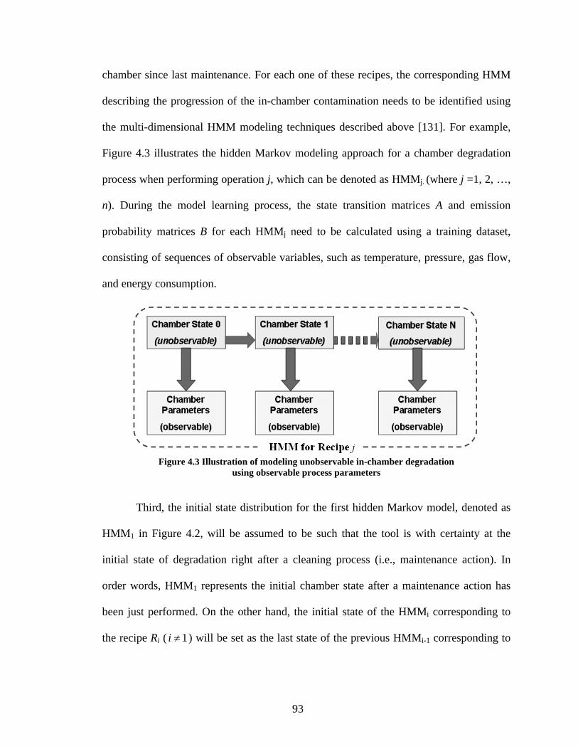
93
chamber since last maintenance. For each one of these recipes, the corresponding HMM
describing the progression of the in-chamber contamination needs to be identified using
the multi-dimensional HMM modeling techniques described above [131]. For example,
Figure 4.3 illustrates the hidden Markov modeling approach for a chamber degradation
process when performing operation j, which can be denoted as HMMj. (where j =1, 2, …,
n). During the model learning process, the state transition matrices A and emission
probability matrices B for each HMMj need to be calculated using a training dataset,
consisting of sequences of observable variables, such as temperature, pressure, gas flow,
and energy consumption.
Figure 4.3 Illustration of modeling unobservable in-chamber degradation
using observable process parameters
Third, the initial state distribution for the first hidden Markov model, denoted as
HMM1 in Figure 4.2, will be assumed to be such that the tool is with certainty at the
initial state of degradation right after a cleaning process (i.e., maintenance action). In
order words, HMM1 represents the initial chamber state after a maintenance action has
been just performed. On the other hand, the initial state of the HMMi corresponding to
the recipe Ri ( 1≠i ) will be set as the last state of the previous HMMi-1 corresponding to

94
the recipe Ri-1 since chamber contamination continuously increases as jobs are processed
in it.
Finally, each HMM will be assumed to be left-to-right, depicting the physical
sense that chamber contamination can only get worse (or stay at its current position) until
a maintenance action is executed. This idea will be further illustrated in more details later
in the simulation study section.
Once this framework has been established, one will be able to use the trained
HMMs and observation variables of the process condition to track and predict the particle
contamination levels of the chamber tools and proactively clean the chamber exactly
when maintenance is required.
4.4. Simulation Study
In order to validate the proposed method, a simulation study is conducted by
following the flowchart shown in Figure 4.4. First, a stochastic degradation process is
simulated, which is assumed to be unobservable to the data acquisition system. However,
this stochastic process will generate observable signals, which will be used to build
HMMs. Then the trained HMM along with observable signals can be used to estimate the
states transition of the underlying degradation process. Finally, the estimation results and
actual degradation process will be compared to verify the modeling accuracy. Two
simulation models will be presented in this section:
1) Single operating condition, which simulates the situation where only
one recipe is used;

95
2) Variable operating conditions, simulating the situation where two or
more recipes are used.
Figure 4.4 Simulation flowchart
4.4.1. Single Operating Condition
In this case study, we assume that there is only one recipe used in the chamber
tool, which implies that the tool degradation process should follow a single pattern
determined by the given recipe. The simulated degradation process is built upon an
exponentially deteriorating curve, as shown in Figure 4.5, plus a normally distributed
random noise factor. The resultant stochastic degradation process is shown in Figure 4.6,
in which the vertical axis is an indicator of degradation level, and the horizontal axis is
simulation time steps. As the value of degradation level indicator increases, the system
performance is getting worse. The exponentially deteriorating trend is employed to imply
a physical system that tends to degrade faster as its condition becomes worse. Note that

96
this assumption is only used to make the simulation more realistic to represent a real
system, which does not constitute a necessary assumption for the modeling approach.
0 100 200 300 400 500 600 700 800 900 10000.5
1
1.5
2
2.5
3
3.5
4
4.5
5
5.5
Simulation Time Steps
Deg
rada
tion
Cur
ve
Figure 4.5 Exponential degradation curve under single operating condition
0 100 200 300 400 500 600 700 800 900 1000-1
0
1
2
3
4
5
6
7
Simulation Time Steps
Deg
rada
tion
Leve
l Ind
icat
or
Figure 4.6 Stochastic degradation process under single operating condition

97
As mentioned in section 4.3, we proposed a stratified level of degradation to
represent the state of chamber condition, rather than trying to postulate the exact value of
degradation level indicator. One way to discretize the continuous degradation process is
evenly divide the vertical range into N regions and each of them corresponds to one
degradation state, where N is the number of states used to describe the entire degradation
process. For example, Figure 4.7 illustrates the idea of using 5 stratified states to
represent the stochastic degradation process shown in Figure 4.6, in which the dotted line
represents the discretized state. It can be seen that as the degradation process evolves, the
state number changes from 1 to 5. Furthermore, as we discussed earlier, the exponentially
deteriorating trend mimics the fact that a physical system tends to degrade faster as its
condition becomes worse. Therefore, it can be seen that the duration that the system stays
in a preceding state is longer than that it stays in a succeeding state.
0 100 200 300 400 500 600 700 800 900 1000-1
0
1
2
3
4
5
6
7
Simulation Time Steps
Deg
rada
tion
Leve
l Ind
icat
or/S
tate
Figure 4.7 Stratified degradation states under single operating condition
State # 1
State # 2
State # 3
State # 4
State # 5

98
Ideally, if one can observe the degradation process shown in Figure 4.6 and
further discretize it into stratified states (Figure 4.7), a PdM decision could be easily
made according to the current degradation state. Unfortunately, in most of cases the
degradation process is not directly observable, such as the situation in a chamber tool we
mentioned in the beginning of this chapter. Therefore, one will have to rely on the readily
observable signals emitted from the deteriorating system to infer the underlying
degradation process.
In this simulation model, the observable signals are generated as follows. We
assume that there is one observable variable emitting from the system. This assumption
will only make the simulation model simple, but the HMM modeling procedure will
remain the same if there are more observable variables, provided that an adjusted Baum-
Welch algorithm will be used in multi-sensor cases [131, 132]. Furthermore, we assume
that the observable variable will only contain two types of emission symbols, i.e.,
{ }2,1=V . We denote ‘1’ to represent ‘conforming’ signal and ‘2’ to represent
‘nonconforming’ signal. In reality, the observable signals will be continuous variables in
most cases, such as temperature, pressure, and gas flow, which need to be transformed
into discrete emission symbols by discretization, as we will perform later in the case
study.
In order to use the stochastic process to generate an observable signal, the
following rules will be followed: when the degradation indicator is deviated more than
one standard deviation from its baseline (the exponential curve), the system will generate
‘nonconforming’ signals, i.e., ‘2’. Otherwise, when the degradation indicator is within
one standard deviation of its baseline, the observable signal will be generated according

99
to its current degradation states. As we assume that in the early states the system is in
‘good’ condition, it tends to generate more ‘conforming’ signals rather than
‘nonconforming’ ones; and as the system degrades, more ‘nonconforming’ signals will
occur. Table 4.1 shows one such example of emission probability table, in which each
row corresponds to a system degradation state, and each column corresponds to the
probability of generating one type of emission symbols. For instance, when the system is
in state # 1 (best state), it has 90% probability to generate ‘conforming’ signals denoted
by ‘1’, and 10% probability to generate ‘nonconforming’ signals denoted by ‘2’;
however, when the system deteriorates to the fifth state (worst state), it only has 10%
probability to generate ‘conforming’ signals and 90% probability to generate
‘nonconforming’ signals.
System State
Observable Symbols
1 2 1 0.9 0.1 2 0.7 0.3 3 0.5 0.5 4 0.3 0.7 5 0.1 0.9
Table 4.1 Emission probability table under single operating condition
Once we have established the underlying degradation states and the emission
probability table, a series of observable emission symbols can be generated using the
simulation model, which will be used to train a HMM. In HMM learning, the number of
states used to model the process is a trade-off between modeling accuracy and
computational cost. In speech recognition [128] and machine condition monitoring [133]
applications, 3-state HMMs are often used, which generally yield results that are good
enough to represent the corresponding processes. However, since our modeling purpose

100
is to facilitate maintenance decision-making, 3-state HMM does not give enough
representation to an entire degradation process. For example, if state # 1 denotes the
initial state of chamber performance right after maintenance and state # 3 denotes the
state of chamber performance, which is no longer qualified to produce any products.
Then the only choice for conducting maintenance is state # 2, which will lead to a trivial
solution of maintenance decision-making. Therefore, in order to accommodate the
maintenance decision-making representation, but not to increase the computation cost too
much, we will try to model the degradation process using 4-state, 5-state and 6-state
HMMs and select the one that yields the maximum likelihood estimates.
Figure 4.8 Illustration of 5-state unidirectional HMM
Furthermore, the topology of HMM used in this research will be unidirectional as
shown in Figure 4.8. Each circle represents a degradation state. Edges along with arrows
represent the directions of state transitions, and then the likelihood of this transition
happens is depicted along with each edge. For instance, P11 means the probability that
state # 1 will stay at its current state; P12 means the probability that state # 1 will transit to
state # 2, P13 means the probability that state # 1 will transit to state # 3, and so on. It can
be seen that this is a unidirectional HMM, which only contains transitions from ‘lower’
states to ‘higher’ states, or unchanged states. The physical interpretation of this uni-
directionality lies in that tool performance will either be getting worse or remain the

101
same, but it cannot become better unless the chamber is maintained, in which case we
assume that the tool state will be reset to its initial state # 1.
First, let us use a unidirectional 4-state HMM to model the degradation process.
The transition probability matrix and emission probability matrix can be estimated using
Baum-Welch algorithm [129]. Due to the nature of Baum-Welch algorithm, multiple
trials have been performed with random initialization and the model with the maximum
logarithm likelihood value is selected, as shown below. For this particular model, the
logarithm likelihood is -508.37.
Transition probability (4-state)
⎥⎥⎥⎥
⎦
⎤
⎢⎢⎢⎢
⎣
⎡
=
10000038.09962.00000040.09960.00000025.09975.0
A
Emission probability (4-state)
⎥⎥⎥⎥
⎦
⎤
⎢⎢⎢⎢
⎣
⎡
=
8897.01103.05843.04157.03203.06797.01056.08944.0
B
The trained HMM can be used along with the observable signal to estimate the
underlying state transition, which is plotted against the original degradation indicator as
well as the stratified states, as shown in Figure 4.9, in which the solid line represents the
estimated states. It can be seen that the estimated states follow the same pattern of
stratified states very well except the last state due to the deficiency of number of states. In
order to evaluate the performance of this model quantitatively, the sum of squared error
(SSE) of using stratified state to represent original degradation indicator is calculated as a
benchmark reference value
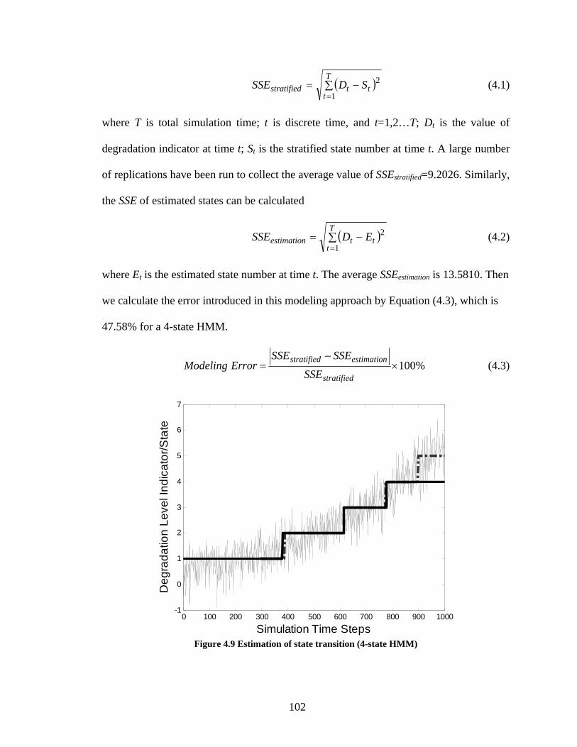
102
( )∑ −==
T
tttstratified SDSSE
1
2 (4.1)
where T is total simulation time; t is discrete time, and t=1,2…T; Dt is the value of
degradation indicator at time t; St is the stratified state number at time t. A large number
of replications have been run to collect the average value of SSEstratified=9.2026. Similarly,
the SSE of estimated states can be calculated
( )∑ −==
T
tttestimation EDSSE
1
2 (4.2)
where Et is the estimated state number at time t. The average SSEestimation is 13.5810. Then
we calculate the error introduced in this modeling approach by Equation (4.3), which is
47.58% for a 4-state HMM.
%100×−
=stratified
estimationstratified
SSE
SSESSEErrorModeling (4.3)
0 100 200 300 400 500 600 700 800 900 1000-1
0
1
2
3
4
5
6
7
Simulation Time Steps
Deg
rada
tion
Leve
l Ind
icat
or/S
tate
Figure 4.9 Estimation of state transition (4-state HMM)

103
Next, we increase the number of states for HMMs. We follow the same procedure
as mentioned in 4-state HMM modeling to get 5-state and 6-state HMMs with logarithm
likelihood -494.70 and -498.12 respectively. The characteristic parameters for these two
models are as follows:
5-state HMM:
Transition probability
⎥⎥⎥⎥⎥⎥
⎦
⎤
⎢⎢⎢⎢⎢⎢
⎣
⎡
=
100000080.09920.000000065.09935.000000044.09956.000000025.09975.0
A
Emission probability
⎥⎥⎥⎥⎥⎥
⎦
⎤
⎢⎢⎢⎢⎢⎢
⎣
⎡
=
9270.00730.07199.02801.05212.04788.03083.06917.01112.08888.0
B
6-state HMM:
Transition probability
⎥⎥⎥⎥⎥⎥⎥⎥
⎦
⎤
⎢⎢⎢⎢⎢⎢⎢⎢
⎣
⎡
=
1000000216.09784.0000000096.09904.0000000059.09941.0000000041.09959.0000000029.09971.0
A
Emission probability
⎥⎥⎥⎥⎥⎥⎥⎥
⎦
⎤
⎢⎢⎢⎢⎢⎢⎢⎢
⎣
⎡
=
9051.00949.07975.02025.07016.02984.05018.04982.02703.07297.00893.09107.0
B

104
Again, the estimated states can be obtained through Viterbi algorithm [130] using
trained HMMs and observable variables, which are plotted in Figures 4.10 and 4.11. In
addition, the modeling accuracy is evaluated using Equations (4.2) and (4.3):
5-state HMM:
SSEestimation = 9.3384 & Modeling Error = 1.48%
6-state HMM:
SSEestimation = 10.0319 & Modeling Error = 9.01%
0 100 200 300 400 500 600 700 800 900 1000-1
0
1
2
3
4
5
6
7
Simulation Time Steps
Deg
rada
tion
Leve
l Ind
icat
or/S
tate
Figure 4.10 Estimation of state transition (5-state HMM)

105
0 100 200 300 400 500 600 700 800 900 1000-1
0
1
2
3
4
5
6
7
Simulation Time Steps
Deg
rada
tion
Leve
l Ind
icat
or/S
tate
Figure 4.11 Estimation of state transition (6-state HMM)
By comparing the likelihood of above models, the 5-state model will be selected,
which offers a better representation of the underlying degradation process as well as the
least modeling errors. Therefore, it has been shown that HMM is able to identify the
stratified degradation states by using the observable signals under single operating
condition.
4.4.2. Variable Operating Conditions
The above simulation has shown that if a HMM is selected properly, it is able to
model the degradation process by assuming a stratified level of states when a single
operating condition exists. In the following simulation model, we would like to verify
that the HMMs are also able to model the varying operating conditions as encountered in
the semiconductor manufacturing process where multiple recipes will be executed in the
same chamber tool.

106
Similar to the simulation model built for a single operating condition, we will
construct a degradation curve as shown in Figure 4.12. Different from the single
operating condition case shown in Figure 4.5, we will introduce varying degradation
curve due to the variable operating conditions, i.e., different recipes may have different
impacts on the tool degradation. It can be seen from Figure 4.12 that the tool is firstly
deteriorating at a slower rate during the time when Recipe # 1 is executed, and a faster
rate for Recipe # 2. The tool degradation curve will be brought back to its original
condition as a maintenance action is performed. In addition, the uncertainty has been
added to the degradation curve to simulate the stochastic nature of the degradation
process, yielding the result shown in Figure 4.13.
0 200 400 600 800 1000 1200 1400 1600 1800 2000
0
2
4
6
8
10
Simulation Time Steps
Deg
rada
tion
Cur
ve
Figure 4.12 Degradation curve under variable operating conditions
Recipe # 1
Recipe # 2
Maintenance

107
0 200 400 600 800 1000 1200 1400 1600 1800 2000
0
2
4
6
8
10
Simulation Time Steps
Deg
rada
tion
Leve
l Ind
icat
or
Figure 4.13 Stochastic degradation process under variable operating conditions
0 200 400 600 800 1000 1200 1400 1600 1800 2000
0
2
4
6
8
10
Simulation Time Steps
Deg
rada
tion
Leve
l Ind
icat
or/S
tate
Figure 4.14 Stratified degradation state under variable operating conditions
Recipe # 1
Recipe # 2
Maintenance
Recipe # 1
Recipe # 2
Maintenance

108
System State
Recipe # 1 Observable
Symbols
Recipe # 2 Observable
Symbols 1 2 1 2
1 0.9 0.1 0.8 0.2 2 0.7 0.3 0.6 0.4 3 0.5 0.5 0.5 0.5 4 0.3 0.7 0.4 0.6 5 0.1 0.9 0.2 0.8
Table 4.2 Emission probability table under variable operating conditions
We adopt the same idea of using stratified states to represent the continuous
degradation process, and divide the entire process into discrete states. It can be seen from
Figure 4.14 that the initial state of Recipe # 2 should be seamlessly connected to the last
state of Recipe # 1, indicating the continuous deterioration of tool performance.
The observable variable will be generated in the same way as it was in the single
operating condition case. That is, when the degradation indicator is deviated more than
one standard deviation from its baseline (the degradation curve), the system will generate
‘nonconforming’ signals denoted by ‘2’. Otherwise, when the degradation indicator is
within one standard deviation of its baseline, the observable signal will be generated
according to its current degradation states, for which emission probabilities will be
assigned to each of them as given in Table 4.2. Next, the simulated observable signals
will be used to train two HMMs for Recipe # 1 and Recipe # 2 respectively. We need to
undergo the same model selection procedure by comparing different models, and select
the one that offers the maximum likelihood. The resultant transition probability and
emission probability matrices for two recipes are given as follows:

109
Recipe # 1:
Transition probability
⎥⎥⎥⎥⎥⎥
⎦
⎤
⎢⎢⎢⎢⎢⎢
⎣
⎡
=
100000102.09898.000000053.09947.000000055.09945.000000025.09975.0
1A
Emission probability
⎥⎥⎥⎥⎥⎥
⎦
⎤
⎢⎢⎢⎢⎢⎢
⎣
⎡
=
8469.01531.06887.03113.05075.04925.03046.06954.01073.08927.0
1B
Recipe # 2:
Transition probability
⎥⎥⎥⎥⎥⎥
⎦
⎤
⎢⎢⎢⎢⎢⎢
⎣
⎡
=
100000101.09899.000000090.09910.000000053.09947.000000033.09967.0
2A
Emission probability
⎥⎥⎥⎥⎥⎥
⎦
⎤
⎢⎢⎢⎢⎢⎢
⎣
⎡
=
8261.01739.05587.04413.05332.04668.04067.05933.02151.07849.0
2B
The underlying state transition can be estimated using the trained HMMs along
with observable variables, as shown in Figure 4.15. The solid line represents the
estimated states, which follows the same pattern as ‘real’ stratified states. To
quantitatively evaluate the modeling accuracy, Equation (4.1) is used to establish the
benchmark value SSEstratified = 14.5696, and Equation (4.2) to calculate SSEestimation =
15.0610. The modeling error is 3.37% given by Equation (4.3). The results shown here

110
verify that by concatenating two or more HMMs, a continuous degradation process can
be modeled using stratified degradation levels and can be estimated using HMMs. The
constraint that has to be applied in the modeling process is that the initial state of
succeeding HMMs must be the last state of its preceding HMMs.
0 200 400 600 800 1000 1200 1400 1600 1800 2000
0
2
4
6
8
10
Simulation Time Steps
Deg
rada
tion
Leve
l Ind
icat
or/S
tate
Figure 4.15 Estimation of state transition under variable operating conditions
4.5. Case Study
Section 4.3 proposed a methodological framework of using HMM to model the
progression of unobservable chamber degradation under multi-operations, which has
been validated using simulation study in section 4.4. The method will be able to provide
an insight about how the chamber tool goes through a stratified deterioration process over
time. As mentioned before, the ‘stratified’ contamination level is employed in this
research to avoid attempting to estimate exact number of particles in the chamber, which
may not be feasible or even necessary. In the following, a set of industrial data set will be
used to illustrate and verify this method.

111
A set of process data is collected from a chamber tool, which consists of two
consecutive operations with two recipes. During the entire production, nine process
parameters and the succeeding metrology measurement are always being monitored,
which means these parameters are observable. However, the underlying chamber
degradation is not directly monitored or measured, which needs to be estimated by
applying the proposed HMMs based method to observable parameters.
In order to accommodate with HMM modeling approach, data preprocessing
needs to be firstly conducted to convert raw data into observation symbols, which
includes data separation, features extraction and data discretization, as described below:
1) Recipe level data separation
Original dataset is divided into two subsets based on recipe
information, and each of them will formulate a HMM
2) Wafer level data separation
Observation sequences are obtained by separating data according to
wafer production
A few observation sequences should be truncated to have the uniform
length
3) Feature Extraction
Deviations from normal values are extracted out of raw data,
representing influential factors of product quality
4) Emission symbol generation
Continuous observations are discretized into discrete emission
symbols

112
Figure 4.16 HMM learning curve.
X-axis: number of iterations; Y-axis: logarithmic likelihood
As mentioned in section 4.4, since the frequently used 3-state HMM is not
adequate for maintenance decision-making purpose, a higher order model will be sought
in this study. 4-state, 5-state and 6-state HMMs will be compared to obtain a model that
has the maximum likelihood estimates. The results show that 5-state model offers the
maximum logarithm likelihood of -1500 for this particular dataset. Care must be taken in
modeling the HMMs using Braun-Welch algorithm, because one of the problems of
Braum-Welch algorithm (which is a generalized Expectation-Maximization algorithm) is
that it is only able to discover a local optimum solution. Therefore, random initialization
has been applied, and the model with the maximum likelihood will be chosen so as to
avoid local optimum by comparing the logarithmic likelihood. The learning curve of
HMM is shown in Figure 4.16.
Since the training data contains information for two recipes, the learning process
will give us two HMM models with model parameters, such as state transition matrices A
0 5 10 15 20 25-5500
-5000
-4500
-4000
-3500
-3000
-2500
-2000
-1500
-1000

113
and emission probability matrices B. We denote these two HMM models as HMM1 and
HMM2. The transition probability matrices for two given recipes are as follows:
Recipe # 1:
⎥⎥⎥⎥⎥⎥
⎦
⎤
⎢⎢⎢⎢⎢⎢
⎣
⎡
=
100000256.09744.00000009.00119.09872.00000200.00544.09256.00000086.00195.09719.0
1A
Recipe # 2:
⎥⎥⎥⎥⎥⎥
⎦
⎤
⎢⎢⎢⎢⎢⎢
⎣
⎡
=
100007721.02279.00000170.02804.07026.0000013.00053.00254.09680.00000000.06853.03147.0
2A
The next step is to solve a decoding problem using models HMM1 and HMM2 to
estimate the underlying tool degradation states, which are unobservable to maintenance
decision makers. As mentioned in section 4.2, the most likely state sequence for given
observable parameters is estimated using Viterbi algorithm. One constraint we need to
specify is that the initial state of a HMM is the last state of its preceding HMM as the tool
degradation is a continuous process, unless a chamber cleaning is performed to bring the
tool state back to its initial state # 1.
Figure 4.17 shows a part of the tool state estimation results, in which the X-axis is
observations over time and Y-axis is the tool degradation state. Although 5-states HMMs
has been employed in this case study, it can be seen that the actual tool degradation state
may end up with a number greater than 5. This is because the chamber tool will not be

114
cleaned after each recipe production, and it will be continuously deteriorated as the
production is undergoing. The degradation states then will be accumulated until a
maintenance action is taken.
It can be seen from Figure 4.17 that the tool starts from its initial state (at position
X=0 and Y=1), after R1 recipe is finished, tool state has deteriorated to the point where
X=250 and Y=5. However, the current state is still good enough to produce wafers using
R2 recipe, therefore R2 is executed which keeps driving the tool degradation until the
position where X=500 and Y=9. After that, a maintenance action is called in, and tool
performance is brought back to its initial state with Y=1, the degradation process will
keep going on over time.
Figure 4.17 Chamber deterioration and maintenance
X-axis: observations over time, Y-axis: degradation state
Another important fact that can be learnt from Figure 4.17 is that the tool
degradation has been stratified into discrete levels, rather than estimating the exact
number of particles in the chamber which is impossible or even unnecessary in practice.
The advantage of this stratified modeling is to enable a simple maintenance decision-
making through direct observable signals that have been monitored all the time in the fab.

115
The utilization of this modeling tool to facilitate maintenance decision-making will be
discussed in Chapter 5.
4.6. Conclusions
Directly monitoring of chamber particle contamination is still an unsolved
problem in practice because of expensive cost as well as unreliable monitoring results. In
order to ensure product quality, excessive preventive maintenance has to be performed
that substantially increase the manufacturing cost. In literature, researchers have proposed
using Markov chain to model the semiconductor tool degradation in order to facilitate
maintenance decision-making, but the underlying assumption is not realistic because of
the unobservable nature of tool deterioration states. On the other hand, HMM has been
used to model speech signal, traditional manufacturing tool monitoring, where HMM
modeling techniques have gained many successes; however, it has not been applied to
model the chamber tool degradation process, especially modeling the progression of
degradation under variable operating conditions, i.e., the operation involves different
recipes that have distinct impacts on tool degradations.
This chapter proposed a method of estimating unobservable chamber tool
deterioration using available process information, such as in-situ measurements and
controller readings. In this approach, a single HMM is employed to capture the
degradation within each operation, whilst the progression of degradation between
operations is modeled by concatenating a series of HMMs by setting the initial states of
subsequent HMMs as the last states of their succeeding HMMs. Furthermore, the

116
degradation process is modeled in such a way that tool states would never go backwards,
i.e., from a worse state to a better state unless a maintenance action is performed.
In order to validate the proposed method, a simulation study has been performed,
including two scenarios: single operating condition and variable operating conditions.
The simulation has successfully shown that HMMs are able to model the tool degradation
process with appropriate selected model parameters. In addition, the entire procedure of
implementing this method is presented in a case study, which includes data
preprocessing, HMMs modeling, tool states estimation. A chamber tool consisting
operations of two distinct recipes is selected for this study. Data are collected from nine
observable sensors, and are separated based on recipes and wafer numbers. Next features
have been extracted from raw data, and discretization is performed to generate emission
symbols for HMM training. Through the HMM learning process, two HMMs are trained
to represent the degradation transition under two recipe operations respectively. The
trained models, in turn, can be utilized to estimate the unobservable chamber degradation
state using observable signals. The results of case study has shown that different recipes
undergo the same chamber may have different impact on tool degradations, and each of
them has a clear trend of tool deterioration, which enables one to schedule maintenance
on the right time. Moreover, the method proposed in this chapter provide a possibility
that deteriorated tool may still be qualified to perform certain operations without
comprising the product quality, thus to avoid performing excessive maintenance and
wasting the tool’s remaining useful life.

117
CHAPTER 5
IMPROVED MAINTENANCE DECISION USING PREDICTED PROCESS
CONDITION AND PRODUCT QUALITY INFORMATION
5.1. Introduction
A semiconductor manufacturing system is a highly complicated and integrated
system with many tools and products. The products travel through the same tool groups
repetitively using re-entrant flows. This complexity has been increased since the
introduction of 300mm wafers, which usually involves more than one hundred tools and
requires several months of processing time for a single product. During this complex
manufacturing process, equipment downtime may cause a significant loss of productivity
and profit. In addition, the downtime on a single tool may result in disruptions and idle
time on many other tools in the process flow. Furthermore, even the operational tools
cannot always guarantee to produce chips with satisfactory quality due to the degradation
of tool performance. Thus, extensive efforts have been devoted to improving the
maintenance strategies so as to keep tools in their acceptable operating conditions as well
as to prevent tools from catastrophic failure.
In today’s semiconductor industry, the preventive maintenance along with
reactive maintenance are dominant practice strategies [5]. As discussed in the previous

118
chapters, the preventive maintenance only utilizes the historical reliability information
and/or expert experiences, and bases the maintenance decision on time or usage related
indicators, such as calendar time, processed wafers/operations. The current practices
usually result in maintenance operations that are more frequent than really needed, which
does not only bring excessive intrusion to the normal operations, but also wastes the tools
remaining useful life and the limited maintenance resources. Although significant work
has been done in the area of maintenance decision-making in semiconductor fabs, the
models used in literature usually do not consider the effects of chamber degradation and
yield of different recipes. For example, Yao et al. [95, 134] studied age-based preventive
maintenance scheduling in semiconductor fabs. They proposed a two level hierarchical
modeling structure, with long-term planning at the higher level, and short-term PM
scheduling at the lower level. However, this model does not take into account the
dependencies between the two levels in order to achieve tractability of the solution.
Furthermore, tool degradation, equipment condition monitoring and production
dispatching were not considered in their model. In addition, the Markov degradation
model of the tool is assumed to be already given. Sloan et al. [3, 135] developed a model
that simultaneously determines maintenance and production schedules for a single-stage,
multi-product system. They assumed an analytical character of product yield and tool
degradation which is not the case in reality, and it is neither explicitly described how to
obtain the description of the degradation process, nor the maintenance policy is
optimized.
On the other hand, the PdM, especially the strictly PdM based on predicting
future states of the fabrication tools have demonstrated promising applications in a

119
variety of industrial areas, such as rotating machinery, aerospace systems, chemical
manufacturing, and electrical equipment & electronic components. Therefore, the PdM
approaches taking advantage of the available tool performance and product quality
information to schedule the maintenance activities should be pursued in semiconductor
manufacturing. There are certain research challenges that have prevented the
semiconductor industry from developing and implementing the PdM strategies, such as:
• Modeling of interaction between production and maintenance operations.
Interaction between production and maintenance operations in any
production system is complex and affects strongly the performance of a plant
[4]. This interaction becomes even more intense and important in highly
complex manufacturing facilities, such as semiconductor fabs. Modeling of
such interaction is crucial for obtaining maintenance schedules that will not
be intruding on the normal production process.
• Modeling of the influence of batching and re-entrant events on the product
quality. The significance of modeling of the production processes in order to
obtain optimal, non-intrusive maintenance schedules that use predictive
machine-condition information has been recognized [136], where methods
have been derived to utilize equipment reliability and in-line manufacturing
system status information in order to optimally prioritize and schedule
maintenance operations. However, these methods have been developed only
for traditional, sequential processes that are characteristic for automotive
manufacturing processes.
• Multiple objective optimization. The optimal maintenance scheduling
consists of multiple objectives, such as the maximization of yield, the
minimization of equipment downtime, and the maximization of total profit.
A cost function that incorporates the cost of maintenance operations and

120
benefits of the production process should be formulated in order to achieve
an optimization procedure that would look for optimal maintenance
operations. Furthermore, highly complex and stochastic nature of operations
in a semiconductor fab causes the maintenance optimization problem to be
inevitably complex and non-analytical, which makes traditional optimization
procedures, such as linear programming or gradient based searches,
unfeasible and impractical in reality.
Nevertheless, from the work presented in Chapter 3 and Chapter 4, it can be seen
that the BN based yield prediction approach and the HMM based modeling of chamber
tool degradation can naturally provide an opportunity to use abundant equipment
condition and product quality information to facilitate a more proactive maintenance
decision-making policy. The focus of this chapter is to adapt the research results from
Chapter 3 and Chapter 4 to demonstrate an improved maintenance decision-making
approach.
5.2. Proposed Method
The idea of developing an improved maintenance decision-making tool for the
complex semiconductor manufacturing system will be proposed in this section, which
utilizes the research results from previous chapters. The methodological framework is
depicted in Figure 5.1.

121
Figure 5.1 Methodology framework of improved maintenance decision-making
The data-preprocessing phase will collect and preprocess the in-situ monitoring,
process controller, and product quality data. The activities include but not limited to data
cleaning, consolidation, synchronization, feature extraction, and data discretization if
necessary. Then the two modeling methods presented in Chapter 3 and Chapter 4, i.e.,
BN based yield prediction and HMM based tool degradation estimation, will come into
play.
First, the BN prediction approach discussed in Chapter 3 is able to infer the
station-level yield and system-level yield based on the integrated information flow of
equipment conditions. This enables one to identify stochastic dependencies among
process information and product qualities, as well as to estimate the product quality
distribution prior to the metrology inspection is performed. Thus if the predicted product
quality is going to deteriorate to an unacceptable level, the BN prediction will provide the
production management with an early warning for loss of quality products, which in turn

122
calls for maintenance in place. Note that the input of this model is process information,
and the output is yield estimation.
Second, the HMM based modeling techniques presented in Chapter 4 are capable
of using current available in-situ measurements to predict the level of particle
contamination in chamber tool, which is recognized as one of the major sources of yield
loss. This model uses stratified representation of tool degradation to avoid the prediction
of exact particle counts, which makes the goal feasible but useful in practice. This HMM
based modeling tool can be naturally extended to any fabrication tools with process
variables that are difficult to be monitored directly. Note that the input of this model is
still process information, and the output is the estimation of tool degradation state.
Furthermore, it can be seen from Figure 5.1, the output of chamber tool degradation
model will be fed into BN based yield model, which enables one to relate tool
degradation status with product quality directly. In order words, an enhanced BN model
will be constructed using the same procedure described in Chapter 3, with a minor
modification that includes ‘Tool State’ as one of the variables. The benefit of this model
is that one will be able to make yield prediction by given tool state estimation, and this
combined information will facilitate maintenance decision-making.
Third, using the tool degradation estimation and yield prediction obtained from
integrating the process information, different maintenance scenarios can be evaluated and
compared to determine which action is relatively better in terms of certain criterion,
which is defined by a customized objective function. The objective function can be quite
versatile depending on customer’s targets, such as low cost, high reliability, high yield,
and low downtime. Because of its inherent complex characteristic, it is impossible to

123
express the dynamics of a semiconductor manufacturing process in analytical forms.
Therefore, the discrete event simulation [137] can be a powerful tool to calculate required
metrics for it. In literature [4, 136], simulations of traditional, sequential manufacturing
processes have been constructed so that continuous interactions between equipment
degradation, maintenance operations and production process could be simulated. In
simulating the semiconductor manufacturing process, the sequential nature of the
simulated system will be altered in order to accommodate for batching and re-entrant
operations in which unfinished wafers are grouped into batches and sent back to the
previously visited station for a similar operation. Also, in the simulation, each station will
be assumed to be at a specific state defined by its current degradation level obtained
using the HMM approach. Then the degradation information can be used to determine the
yield using the BN inference.
Finally, with simulation-based yield prediction, the optimal combination of
maintenance actions that will result in the maximum system-level yield can be pursued.
Since the simulation-based yield function will be a non-analytical form that is not
amenable to traditional optimization methods replying on mathematical formulations,
such as the methods presented in [138-140]. The problem will be approached through
heuristic methods, such as Genetic Algorithm (GA) [141], Simulated Annealing [142],
or the combination of them [143]. The interaction between discrete event simulation and
heuristic optimization methods is further illustrated in Figure 5.2. A set of feasible
maintenance solutions (or candidate solutions) is generated by the optimization
subroutine and is fed into the discrete event simulator as an input. The simulation model
evaluates the distribution of the objective function. Based on the average of objective

124
function values, the optimization subroutine produces another generation of candidate
maintenance solutions (state thresholds that trigger PdM). These steps are repeated until a
termination condition is met (certain number of generations passed without
improvements in the objective function, or maximal number of generations is exceeded).
Figure 5.2 Interaction between discrete-event simulation and optimization methods
For instance, if GA is employed to find the optimal PdM policy, the basic idea
behind GA is to imitate an evolutionary process of survival of the fittest. Each candidate
solution is represented by a chromosome and only the candidate solutions resulting in
lowest average costs (as evaluated through simulations) will produce chromosomes that
code candidate solutions for the next generation of solutions. In order to define a GA, one
needs to define chromosomes through which each candidate solution can be represented,
and a set of genetic operations of crossover and mutation that are needed to create a new
generation of candidate solutions [144].
In summary, the methodology framework of finding improved maintenance
decisions using tool degradation estimation and yield prediction results can be executed
in the sequence as follows. Note that some of the steps may be omitted, such as

125
optimization module in case that the searching space is not too large, and it can be
replaced by enumeration, which will be shown in the case study.
1) Data preprocessing
Major task: collect monitoring signals and perform data cleaning,
consolidation, feature extraction, data discretization task according to
specific requirements (input requirements of BN and HMM models)
Input: Raw data
Output: synthesized features for BN and HMM
2) Chamber state estimation
Major task: use HMM based modeling approach to establish HMMs
for each recipe, and estimate the tool degradation state using
observable parameters
Input: process monitoring features
Output: tool degradation state
3) Predictive yield model
Major task: use process parameters and quality measurements to
discover stochastic dependencies, and make probabilistic inference of
yield when new observation of process parameters is available.
Furthermore, establish the direct link between tool degradation and
yield
Input: process monitoring features, quality data, tool degradation state
Output: yield
4) Simulation module

126
Major task: use tool degradation models, yield prediction results to
evaluate different maintenance policies
Input: Tool degradation and corresponding yield, maintenance policy
Output: value of objective function specified by user
5) Optimization module
Major task: generate feasible solutions to be evaluated by simulation
module
Input: best candidate solution in previous iteration
Output: possible maintenance policies
5.3. Case Study
The purpose of this case study is to demonstrate the utilization of BN based yield
prediction model and HMM based tool degradation model for maintenance decision-
making, providing an improved maintenance policy over currently used PM strategy. As
mentioned above, the simulation and optimization module may be involved in the
maintenance decision-making process; however, it is not in the scope of this research.
The simulation-based maintenance decision-making has been reported in dedicated
research work, such as Yang [136] and Zhou [145]. Also, the heuristic optimization
methods can be found with abundant references, such as Deris et al. [146], Sotoh and
Nara [142], and Dahal et al. [143].
For the fab system studied here, it is known that wafers were fabricated using one
single recipe in a chamber tool. Since there is no adequate information about tool
degradation and how the product quality is related to tool performance, the PM tasks had

127
to be scheduled in such a way that chamber must be cleaned once two wafers were
produced to avoid catastrophic tool failures. The fab has suffered from too frequent PM,
which resulted in substantial cost of maintenance resources. Therefore, it is desirable to
develop a PdM strategy, which is able to use the tool performance information as well as
the knowledge of outgoing product quality to facilitate a better maintenance scheduling.
However, as discussed in early chapters, that information is not readily available in the
fab, and has to be derived from other observable information, such as in-situ sensing and
controller data. In this case study, the available information consists of a data set
including nine process parameters, one metrology measurement, the average time
between maintenance for PM scheduling, time to perform a PM cleaning, and normalized
PM cleaning cost.
According to Figure 5.1 and summary in section 5.1, the case study has included
the following steps:
1) Data preprocessing
Data is processed to accommodate BN and HMM training, as
described in Chapter 3 and Chapter 4, namely, feature extraction, data
discretization, emission symbols generation, etc.
2) Chamber state estimation
A HMM is trained using the training data set. The transition
probability matrix of this HMM is as below, which will be used in the
discrete event simulation to represent tool degradation.

128
⎥⎥⎥⎥⎥⎥
⎦
⎤
⎢⎢⎢⎢⎢⎢
⎣
⎡
=
100000256.09744.000000052.09948.00000200.00544.09256.000005068.04932.0
A
Tool degradation is estimated through this trained HMM, and
corresponding tool states over time are combined with training dataset
to feed into BN based yield prediction.
3) Predictive yield model
A BN network has been trained using training data set including tool
degradation state. A part of the network is shown in Figure 5.3.
Figure 5.3 Modified BN structure including ‘Tool State’
With this BN structure and associated CPTs, the yield can be estimated
for different tool states. Table 5.1 shows a one-to-one ‘Tool State’ vs.
‘Yield’ mapping that will be used in simulation model to evaluate the
process yield.

129
Tool State Yield 1 93.00% 2 92.93% 3 77.83% 4 55.83% 5 0.40%
Table 5.1 Tool deterioration states and corresponding yields
4) Simulation module
Discrete event simulation model is used to evaluate the objective
function ( ) rprpclclyy TCTCYieldCCObj ++−= 21 exp , where Cy1 and Cy2
are cost coefficients for yield loss, Ccl and Crp are normalized cost
coefficients for cleaning and repair in one time unit, Tcl and Trp are
total time used for cleaning and repair respectively.
This objective function is set in such a way that it takes into account
the need to achieve highest possible yield, while minimizing the costs
of scheduled and unscheduled maintenance.
The values of simulation parameters are assigned as follows:
Parameter Value Description Ts 24 hours Simulation time Cy1 9000 Linear cost coefficient for yield loss Cy2 2 Exponential cost coefficient for yield loss Ccl 1/min Normalized cost coefficient for cleaning Crp 2/min Normalized cost coefficient for repair tcl 5±1 min Time to complete a cleaning task trp 10±2 min Time to complete a repair task
tTBPM 12±2 min Time between two scheduled PM tasks Table 5.2 Simulation parameters for improved maintenance policies
5) Optimization module
Since feasible solution space is not large (i.e., only four different
candidates), it is not necessary to use heuristic methods, such as

130
Genetic Algorithm, to find an optimal solution. Instead, enumeration
can be used to obtain 4 results through simulation to evaluate different
PdM policies.
6) Simulation results
50 replications for each PdM policy are run to take an average of the
objective values.
The simulation results are shown in Table 5.3.
PdM Policy State 2 State 3 State 4 State 5 Yield 0.93 0.93 0.85 0.77
Tcl 230 188 71 0 Trp 0 0 8 196
Obj. Value 1380.27±26.395 1338.27±16.980 1434.16±36.255 1960.31±69.24 Table 5.3 Simulation results with different PdM policies
From the simulation results, it can be seen that performing maintenance when the
tool condition degrades to state # 3 is the best PdM policy based on the given objective
function, which minimizes the total cost of maintenance and yield loss. In order to
compare with the currently used PM policy in the fab, we calculate the normalized total
maintenance cost during a 24 hours period for all feasible PdM policies as well as the
normalized cost of reactive maintenance (RM) and PM policies, as listed in Table 5.4.
Maintenance Policy
Total Time of Cleaning, Tcl
Total Time of Repair, Trp
Total Maintenance Cost
PdM at State # 2 230 0 230 PdM at State # 3 188 0 188 PdM at State # 4 71 8 87
RM 0 196 392 PM 424 0 424
Table 5.4 Comparison of maintenance cost for different policies

131
The computation of normalized PdM cost and RM cost in Table 5.4 is
straightforward by using the total time of cleaning and repair. For example, if we perform
PdM at State # 4, we know that Tcl = 71 and Trp = 8 from the simulation results shown in
Table 5.3. Therefore the normalized total cost is
8782711 =×+×=+= rprpclcl TCTCCost
However, for the normalized total cost of performing scheduled PM tasks, we
need to estimate the total time of cleaning, which is given by
4245512
6024)()()(
≈×+×
=×+
= clclTBPM
scl tE
tEtETT
and then multiple the normalized cost coefficient of cleaning Ccl =1 to obtain the total
cost of 424.
It can be seen from Table 5.4, by employing the PdM when the system degrades
to State # 3, the normalized total maintenance cost has been lowered by 55.66% during
the entire simulation time. Though PdM at State # 4 is able to provide a solution with
even lower cost, the yield suffers an 8.6% drop. In practice, since yield is an essential
factor in the semiconductor manufacturing environment, PdM at State # 3 is a better
policy for this case study.
One should note that the data used in this case study does not contain equipment
failure events, which means artificial ‘failure’ has to be introduced in order to
demonstrate the proposed methodological framework. In practice, when applying this
method to real fabrication, the equipment monitoring database will definitely provide
failure events that can be more realistic to represent the real-world situation.

132
5.4. Conclusions
Maintenance scheduling and decision-making has been studied by many
researchers and have been successfully used in a variety of industrial applications.
However, due to its inherent complex nature of semiconductor manufacturing process,
the current practices of maintenance are still dominated by preventive maintenance
strategies. Among several major obstacles for employing condition-based maintenance,
the unobservable chamber state and the stochastic relation between tool state and wafer
yield have not been fully studied in literature, which are given feasible solutions and have
been demonstrated using case studies in previous chapters. Therefore, the materials
presented in Chapter 3 and Chapter 4 have naturally lent themselves to an improved
maintenance decision-making scheme, as both the tool degradation state and the yield
prediction are essential to ensure the maintenance decision-making to be successful.
This chapter is intended to propose a methodological framework of intelligent
maintenance using the estimation of unobservable tool deterioration state and the
prediction of yield at different tool states. In this approach, HMM is employed to capture
the degradation within chambers, and then the BN analysis can be incorporated to get
yield information corresponding to each state of degradation. Both the chamber
degradation and yield information provide necessary information for running simulation
to obtain improved maintenance policies. Furthermore, a case study using semiconductor
dataset has been presented to demonstrate the application procedure. The simulation
results show that instead of performing regular PM cleaning, a PdM policy using
predicted chamber degradation as well as yield information is able to reduce the total
maintenance cost by 55.66% while retaining the highest possible yield.

133
CHAPTER 6
CONCLUSIONS AND FUTURE WORK
6.1. Conclusions
Research presented in this thesis has focused on the development of predictive
modeling methods for intelligent maintenance in complex manufacturing processes (e.g.,
semiconductor fabrication process), using the in-process tool performance and the
product quality information.
The relevant literature of predictive maintenance in the semiconductor
environment have been reviewed, which reveals a clear need of PdM, and the inability of
key enabling techniques, such as in-situ particle monitoring that cannot reliably reflect
the real contamination level in chamber tools. Also, from the literature review, several
potential research directions have been identified, which have been addressed in this
doctoral research.
First, a method for integrating fragmented data domains of in-situ sensor readings,
process controller data, and inspection results in a semiconductor fab to predict process
yield has been proposed in Chapter 3. The proposed method utilizes BNs to discover the
complex stochastic relationships among random variables, identify the factors that are
probabilistically influencing future product quality, and make probability inference out of

134
this model by taking new observations. In order to reduce the computational cost, the
SOMs have been applied to discretize continuous data into discrete levels, each of which
represents a group of similar data in the sense of a predefined distance measurement,
such as Euclidean distance. The proposed method has been validated using the simulation
study and the applications to industrial datasets. The case studies show that the stochastic
dependencies among random variables have been successfully discovered without taking
any prior knowledge, enabling the predictive modeling of metrology results. In addition,
the quantitative comparison between inferred results and true value of metrology shows
promising predictive capability, e.g., 99.78% similarity for the case study using the
semiconductor manufacturing data.
Second, the particle contamination prediction using available in-situ measurement
through hidden Markov model to facilitate PdM has been presented in Chapter 4. The
proposed method employs the idea of stratified levels of degradation to model the tool
deterioration process rather than trying to postulate the exact number of particle counts.
Single HMM has been employed to represent the tool degradation process under a single
recipe operation; and the concatenation of multiple HMMs can be used to model the tool
degradation under multiple recipes. In order to validate the proposed method, a
simulation study has been conducted, which showed that HMMs are able to model the
unobservable degradation process under variable operating conditions. Furthermore, a
case study has been employed to demonstrate the proposed method. Through the HMM
learning process, two HMMs are trained to represent the degradation transition under two
recipe operations respectively. The trained models can be utilized to estimate the
unobservable chamber degradation state using observable signals. The results of case

135
study has shown that different recipes undergo the same chamber may have different
impact on tool degradations, and each of them has a clear trend of tool deterioration,
which enables one to schedule maintenance on the right time. Moreover, the method
proposed in this chapter provide a possibility that deteriorated tool may still be qualified
to perform certain operations without comprising the product quality, thus to avoid
performing excessive maintenance and wasting the tool’s remaining useful life.
Finally, an improved maintenance decision-making framework using the
information from the BN inference and from the HMM prediction, through discrete event
simulation and optimization has been presented in Chapter 5. The procedure of
conducting maintenance decision-making have been outlined and demonstrated using a
case study. Although optimization and simulation are not in the scope of this research, a
numerical result was presented to show that how the estimation of stratified chamber
contamination can facilitate maintenance decision-making, in which discrete event
simulation has been utilized, while the optimization module was not included because of
the relatively small searching spaces. It can be seen from the results that different
maintenance strategies can have significant impacts on the total cost of maintenance, and
an improved maintenance decision-making solution would be able to reduce the total
maintenance cost by 55.66% compared to the currently used PM strategy in this case
study, which would in turn benefit the industry for a long-term run.
6.2. Original Contributions
The original contributions of this doctoral research can be summarized as follows.

136
A method of integrating the equipment condition, process controller data, and
metrology results to predict the product quality is proposed and demonstrated in this
research. The SOMs have been utilized to discretize continuous in-process parameters
into discrete values, which will tremendously reduce the computational cost of BN
learning process that is used to discover the stochastic dependences among process
parameters and product quality. This method allows the integration of fragmented and
inhomogeneous data in different domains, and discovers the complex interrelationships
among process variables and product quality. The outcome of this method enables one to
make more accurate and proactive product quality prediction that is different from
traditional methods based on solely inspection results.
The data integration method proposed in this research naturally leads to a
distance-based data organization facilitating quick data search. Since the proposed BN-
based modeling is highly dependent on the similarity comparison between the
current/predicted signature of equipment condition to that in the historical database, data
search has to be performed extensively throughout the probability inference process.
Compared to the time sequential data organization, the proposed distance-based data
organization resulting from SOMs enables one to find similar entries with significantly
reduced search time while without comprising the search accuracy.
A method for predictive maintenance in chamber tools is proposed, using HMMs
to model the progression of particle contamination that is directly unobservable. Rather
than postulating the exact number of particle counts, a stratified level of contaminations
have been employed to make the modeling task feasible. The method enables one to
estimate the condition of the in-chamber particle contamination levels so that
137
maintenance actions can be initiated accordingly based on accurate relations between
condition measurements, levels of in-chamber particle counts and outgoing product
quality. The method is also able to accommodate with the process involving various
operations performed in the same chamber tool. Furthermore, the proposed method can
be correspondingly extended to other manufacturing processes with machine condition
indicators that are difficult to be observed directly as well as operating under various
conditions.
Finally, a methodological framework of predictive modeling for intelligent
maintenance decision-making by coherently considering product quality and tool
degradation is proposed and demonstrated in this research. The BN based yield prediction
and the HMM based tool degradation estimation provide the fundamental necessities that
enable one to make proactive maintenance decision in a complex manufacturing
environment.
6.3. Future Work
Possible future work beyond the research presented in this report can be
summarized as follows.
In modeling the stochastic dependencies of random variables, a static Bayesian
network has been applied in this research. However, static BN ignores the temporal
dynamics of the modeled system, which may contain more fruitful insights of the
interrelations between tool monitoring parameters and product quality. Therefore, a
dynamic BN approach may be researched in future research to incorporate temporal
information for multivariate stochastic modeling. Furthermore, both static and dynamic

138
BNs have fixed structures, which are not able to accommodate rapid process changes
over time. A stochastic method that is capable of making probability inferences as well as
capturing the rapid process changes should be pursued.
HMM based degradation modeling for chamber tool has been demonstrated in
this research, which can use stratified contamination levels to keep tracking the tool
deterioration states. However, it can be seen that the number of stratified states used to
represent the HMM is an important parameter, which is currently determined based on
previous experience on HMM applications in other areas. Therefore, a rigorous method
that can provide an optimal number of states would be pursued.
As mentioned earlier, although the simulation modeling and optimization methods
are not in the scope of this research, it can be seen that using heuristic optimization plus
discrete event simulation may take quite long time to obtain a maintenance decision,
which prevents the use of proposed method online. Thus, a more interactive, fast
converging, and near-real-time maintenance decision system for semiconductor
manufacturing is desired, and should be investigated.
Finally, it has been demonstrated in this research that the estimation of tool
degradation along with predictive yield models can be used to achieve an improved
maintenance decision on single equipment, but the complex interaction of numerous
equipment, the interaction of job dispatching and scheduling with maintenance would
introduce more challenging problem, which may be of interest for future exploration.

139
BIBLIOGRAPHY
[1] P. Van Zant, Microchip fabrication, 5th ed. New York: McGraw-Hill, 2004.
[2] A. V. Ferris-Prabhu, Introduction to Semiconductor Device Yield Modeling: Artech House, Inc., 1992.
[3] T. W. Sloan and J. G. Shanthikumar, "Using in-line equipment condition and yield information for maintenance scheduling and dispatching in semiconductor wafer fabs," Scheduling and Logistics on Semiconductor Manufacturing, IIE Transactions (Institute of Industrial Engineers), vol. 34, pp. 191-209, 2002.
[4] Z. M. Yang, Q. Chang, D. Djurdjanovic, J. Ni, and J. Lee, "Maintenance priority assignment utilizing on-line production information," Japan-USA Symposium on Flexible Automation, 2004.
[5] D. Djurdjanovic and Y. Liu, "Survey of Predictive Maintenance Research and Industry Best Practice," University of Michigan, Ann Arbor, MI 2006.
[6] S. Montgomery, "Higher profits from intelligent semiconductor equipment maintenance," Future Fab Intl., vol. 8, 2000.
[7] R. K. Mobley, An introduction to predictive maintenance, 1st ed.: Van Nostrand Reinhold, 1990.
[8] N. I. Shaikh and V. V. Prabhu, "Intelligent condition-based maintenance of reactive ion etching process," in Smart Engineering System Design: Neural Networks, Fuzzy Logic, Evolutionary Programming, Complex Systems and Artificial Life - Proceedings of the Artificial Neural Networks in Engineering Conference, Nov 2-5 2003, St. Louis, MO., United States, 2003, pp. 927-932.
[9] R. C. M. Yam, P. W. Tse, L. Li, and P. Tu, "Intelligent predictive decision support system for condition-based maintenance," International Journal of Advanced Manufacturing Technology, vol. 17, pp. 383-391, 2001.
[10] R. B. Randall, "State of the Art in Monitoring Rotating Machinery - Part 1," Sound and Vibration, vol. 38, pp. 14-21, 2004.

140
[11] R. B. Randall, "State of the art in monitoring rotating machinery - Part 2," Sound and Vibration, vol. 38, pp. 10-17, 2004.
[12] S. Wegerich, "Similarity-based modeling of vibration features for fault detection and identification," Sensor Review, vol. 25, pp. 114-122, 2005.
[13] S. Velarde-Suarez, R. Ballesteros-Tajadura, and J. P. Hurtado-Cruz, "A predictive maintenance procedure using pressure and acceleration signals from a centrifugal fan," Applied Acoustics, vol. 67, pp. 49-61, 2006.
[14] B. Al-Najjar, "Accuracy, effectiveness and improvement of vibration-based maintenance in paper mills: case studies," Journal of Sound and Vibrations, vol. 229, pp. 389-410, 2000.
[15] S. Orhan, N. Akturk, and V. Celik, "Vibration monitoring for defect diagnosis of rolling element bearings as a predictive maintenance tool: Comprehensive case studies," NDT and E International, vol. 39, pp. 293-298, 2005.
[16] C. S. Byington and A. K. Garga, "Data Fusion for Developing Predictive Diagnostics for Electromechanical Systems," in Handbook of Sensor Fusion: L. D. Hall and J. Llinas (Eds.), CRC Press,, 2000, pp. 23-1 - 23-31.
[17] G. Yu, H. Qiu, D. Djurdjanovic, and J. Lee, "Feature Signature Prediction of a Boring Process Using Neural Network Modeling with Confidence Bounds," accepted for publication in the International Journal of Advanced Manufacturing Technology, Paper No. 2946, 2005.
[18] J. Liu, D. Djurdjanovic, J. Ni, N. Casoetto, and J. Lee, "Similarity Based Method for Manufacturing Process Performance Prediction and Diagnosis," submitted to Computers in Industry, Paper no. COMIND-D-06-00035, 2006.
[19] C.-C. Lin and H.-Y. Tseng, "A neural network application for reliability modelling and condition-based predictive maintenance," International Journal of Advanced Manufacturing Technology, vol. 25, pp. 174-179, 2005.
[20] H. M. Ertunc, K. A. Loparo, and H. Ocak, "Tool wear condition monitoring in drilling operations using hidden Markov models (HMMs)," International Journal of Machine Tools & Manufacture, vol. 41, pp. 1363-84, 2001.
[21] W. Litao, M. G. Mehrabi, and E. Kannatey-Asibu, Jr., "Hidden Markov model-based tool wear monitoring in turning," Transactions of the ASME. Journal of Manufacturing Science and Engineering, vol. 124, pp. 651-8, 2002.
[22] K. R. Cooper, J. Elster, M. Jones, and R. G. Kelly, "Optical fiber-based corrosion sensor systems for health monitoring of aging aircraft," in Autotestcom 2001, Aug 20-23 2001, Valley Forge, PA, 2001, pp. 847-856.

141
[23] V. K. Varadan, "Wireless microsensors for health monitoring of aircraft structures," in MEMS Components and Applications for Industry, Automobiles, Aerospace, and Communication II, Jan 28-29 2003, San Jose, CA, United States, 2003, pp. 175-188.
[24] T. Brotherton, P. Grabill, D. Wroblewski, R. Friend, B. Sotomayer, and J. Berry, "A testbed for data fusion for engine diagnostics and prognostics," in 2002 IEEE Aerospace Conference Proceedings, 9-16 March 2002, Big Sky, MT, USA, 2002, pp. 6-3029 BN - 0 7803 7231 X.
[25] A. Volponi, "Data fusion for enhanced aircraft engine prognostics and health management," Pratt & Whitney, East Harffort, Connecticut 2005.
[26] P. Knight, J. Cook, and H. Azzam, "Intelligent management of helicopter health and usage management systems data," Proceedings of the Institution of Mechanical Engineers, Part G: Journal of Aerospace Engineering, vol. 219, pp. 507-524, 2005.
[27] R. Callan and B. Larder, "The development and demonstration of a probabilistic diagnostic and prognostic system (ProDAPS) for gas turbines," in 2002 IEEE Aerospace Conference Proceedings, 9-16 March 2002, Big Sky, MT, USA, 2002, pp. 6-3083 BN - 0 7803 7231 X.
[28] D. C. Swanson, "A general prognostic tracking algorithm for predictive maintenance," in 2001 IEEE Aerospace Conference Proceedings, 10-17 March 2001, Big Sky, MT, USA, 2001, pp. 2971-7 BN - 0 7803 6599 2.
[29] G. J. Kacprzynski, A. Sarlashkar, M. J. Roemer, A. Hess, and W. Hardman, "Predicting remaining life by fusing the physics of failure modeling with diagnostics," JOM, vol. 56, pp. 29-35, 2004.
[30] C. S. Byington, M. J. Roemer, and T. Galie, "Prognostic enhancements to diagnostic systems for improved condition-based maintenance [military aircraft]," in 2002 IEEE Aerospace Conference Proceedings, 9-16 March 2002, Big Sky, MT, USA, 2002, pp. 6-2815 BN - 0 7803 7231 X.
[31] C. S. Byington, P. W. Kalgren, R. Johns, and R. J. Beers, "Embedded diagnostic/prognostic reasoning and information continuity for improved avionics maintenance," in AUTOTESTCON 2003. Proceedings. IEEE Systems Readiness Technology Conference, 22-25 Sept. 2003, Anaheim, CA, USA, 2003, pp. 320-9 BN - 0 7803 7837 7.
[32] M. J. Roemer, E. O. Nwadiogbu, and G. Bloor, "Development of diagnostic and prognostic technologies for aerospace health management applications," in 2001 IEEE Aerospace Conference Proceedings, 10-17 March 2001, Big Sky, MT, USA, 2001, pp. 3139-47 BN - 0 7803 6599 2.

142
[33] C. E. Jaske, J. A. Beavers, and N. G. Thompson, "Improving plant reliability through corrosion monitoring," Corrosion Prevention and Control, vol. 49, pp. 3-12, 2002.
[34] N. Bolf, "Application of infrared thermography in chemical engineering," Kemija u industriji/Journal of Chemists and Chemical Engineers, vol. 53, pp. 549-555, 2004.
[35] A. Hoover, "Using ultrasonics in predictive maintenance," Plant Engineering (Barrington, Illinois), vol. 58, pp. 48-50, 2004.
[36] M. A. Sharif and R. I. Grosvenor, "Process plant condition monitoring and fault diagnosis," Proceedings of the Institution of Mechanical Engineers, Part E: Journal of Process Mechanical Engineering, vol. 212, pp. 13-30, 1998.
[37] D. R. Lewin, "Predictive maintenance using PCA," in ADCHEM '94. IFAC Symposium: Advanced Control of Chemical Processes, 25-27 May 1994, Control Engineering Practice, Kyoto, Japan, 1995, pp. 415-21.
[38] V. Venkatasubramanian, R. Rengaswamy, K. Yin, and S. N. Kavuri, "A review of process fault detection and diagnosis part I: Quantitative model-based methods," Computers and Chemical Engineering, vol. 27, pp. 293-311, 2003.
[39] V. Venkatasubramanian, R. Rengaswamy, and S. N. Kavuri, "A review of process fault detection and diagnosis part II: Qualitative models and search strategies," Computers and Chemical Engineering, vol. 27, pp. 313-326, 2003.
[40] V. Venkatasubramanian, R. Rengaswamy, S. N. Kavuri, and K. Yin, "A review of process fault detection and diagnosis part III: Process history based methods," Computers and Chemical Engineering, vol. 27, pp. 327-346, 2003.
[41] P. Ralston, G. DePuy, and J. H. Graham, "Computer-based monitoring and fault diagnosis: A chemical process case study," ISA Transactions, vol. 40, pp. 85-98, 2001.
[42] Y. Han and Y. H. Song, "Condition monitoring techniques for electrical equipment-a literature survey," IEEE Transactions on Power Delivery, vol. 18, pp. 4-13, 2003/01/ 2003.
[43] S. Nandi and H. A. Toliyat, "Condition monitoring and fault diagnosis of electrical machines - a review," Proceedings of the 1999 IEEE Industry Applications Conference - 34th IAS Annual Meeting, Oct 3-Oct 7 1999, Conference Record - IAS Annual Meeting (IEEE Industry Applications Society), vol. 1, pp. 197-204, 1999.
[44] L. Mokhnache, C. Kada, A. Boubakeur, and N. N. Said, "Condition monitoring of fuzzy logic system for oil insulated transformer diagnosis," International Journal of COMADEM, vol. 8, pp. 13-15, 2005.

143
[45] D. Bansal, D. J. Evans, and B. Jones, "A real-time predictive maintenance system for machine systems," International Journal of Machine Tools and Manufacture, vol. 44, pp. 759-766, 2004.
[46] D. Bansal, D. J. Evans, and B. Jones, "Application of a real-time predictive maintenance system to a production machine system," International Journal of Machine Tools and Manufacture, vol. 45, pp. 1210-1221, 2005.
[47] F. M. Discenzo, P. J. Unsworth, K. A. Loparo, and H. O. Marcy, "Self-diagnosing intelligent motors: a key enabler for next generation manufacturing systems," in IEE Colloquium Intelligent and Self-Validating Sensors, 21 June 1999, Oxford, UK, 1999, pp. 3-1.
[48] F. Discenzo, F. Maturana, R. Staron, P. Tichy, P. Slechta, and V. Marik, "Prognostics and Control Integration with Dynamic Reconfigurable Agents," LASME transactions, vol. 1, 2004.
[49] F. M. Discenzo, F. P. Maturana, and D. Chung, "Managed Complexity in An Agent-based Vent Fan Control System Based on Dynamic Re-configuration," in International Conference on Complex Systems (ICCS2002), Nashua, NH, 2002.
[50] M. Fu, S. I. Marcus, and E. Fernandez-Gaucherand, "Survey of Current Best Practices in Preventive Maintenance Scheduling in Semiconductor Manufacturing," University of Maryland, University of Cincinnati, SRC project technical report 2002.
[51] M. Lebold, K. Reichard, P. Hejda, J. Bezdicek, and M. Thurston, "A Framework for Next Generation Machinery Monitoring and Diagnostics," in 56th Meeting of the Society for Machinery Failure Prevention Technology, 2002.
[52] M. Lebold, K. Reichard, C. S. Byington, and "OSA-CBM Architecture Development with Emphasis on XML Implementations," in Maintenance and Reliability Conference (MARCON), 2002.
[53] M. G. Thurston, "An open standard for Web-based condition-based maintenance systems," Valley Forge, PA, USA, 2001, pp. 401-15.
[54] M. Lebold, K. Reichard, and D. Boylan, "Using DCOM in an open system architecture framework for machinery monitoring and diagnostics," in IEEE Aerospace Conference, 2003, pp. 1227–1235.
[55] K. M. Takahashi and J. E. Daugherty, "Current capabilities and limitations of in situ particle monitors in silicon processing equipment," Journal of Vacuum Science & Technology A: Vacuum, Surfaces, and Films, vol. 14, pp. 2983-2993, 1996.
[56] H. Miyashita, T. Kikuchi, Y. Kawasaki, Y. Katakura, and N. Ohsako, "Particle measurements in vacuum tools by in situ particle monitor," Journal of Vacuum

144
Science & Technology A (Vacuum, Surfaces, and Films), vol. 17, pp. 1066-70, 1999/05/ 1999.
[57] A. S. Perel, L. Stone, V. M. Benveniste, and W. K. Loizides, "In-situ monitoring on an ion implanter," U. S. P. V. T. D. NewsEdge, Ed., 2005.
[58] W. Grählert, I. Dani, G. Mäder, O. Throl, K. Pietsch, R. Hellriegel, E. Marx, and V. Hopfe, "In-situ Monitoring of CVD Process Tools by Fourier-Transform Infrared Spectroscopy," in 6th AEC/APC Conference, Jury's Hotel Ballsbridge Dublin, Ireland, 2005.
[59] R. Williams, E. Wickesberg, R. Jacques, M. Bonin, and D. Holve, "Evaluation of the `HiVol' above-wafer in-situ particle monitoring sensor," in Advanced Semiconductor Manufacturing Conference and Workshop, 2000 IEEE/SEMI, 2000, pp. 302-311.
[60] N. Ito, T. Moriya, F. Uesugi, S. Moriya, M. Aomori, Y. Kato, and M. Tachibana, "The application of in situ monitor of extremely rarefied particle clouds grown thermally above wafers by using laser light scattering method to the development of the mass-production condition of the tungsten thermal chemical vapor deposition," Journal of Vacuum Science and Technology, Part A: Vacuum, Surfaces and Films, vol. 19, pp. 1248-1253, 2001.
[61] J. Yan, D. Seif, S. Raghavan, H. J. Barnaby, B. Vermeire, T. Peterson, and F. Shadman, "Sensor for monitoring the rinsing of patterned wafers," IEEE Transactions on Semiconductor Manufacturing, vol. 17, pp. 531-537, 2004.
[62] S. L. Morton, F. L. Degertekin, and B. T. Khuri-Yakub, "Ultrasonic sensor for photoresist process monitoring," IEEE Transactions on Semiconductor Manufacturing, vol. 12, pp. 332-9, 1999/08/ 1999.
[63] S. Cho, L. Henn-Lecordier, A. S. Y. Xu, T. Gougousi, Y. Liu, J. N. Kidder, and G. W. Rubloff, "Real-Time In-Situ Metrology to Drive Real-Time APC," in 2003 AEC/APC Symposium, USA, 2003.
[64] J. Tanaka, A. Kagoshima, D. Shiraishi, H. Yamamoto, and M. Yoshigai, "Etch-Process Monitoring Using Optical Emission Spectra of Process Plasma," in 2003 AEC/APC Symposium, USA, 2003.
[65] E. J. Johnson, P. V. Hyer, P. W. Culotta, and I. O. Clark, "Evaluation of infrared thermography as a diagnostic tool in CVD applications," Journal of Crystal Growth, vol. 187, pp. 463-473, 1998.
[66] L. Karuppiah and B. Swedek, "Overview of CMP Process Control Strategies," Proc. CMP-MIC, 2006.

145
[67] J. Tang, D. Dornfeld, S. K. Pangrle, and A. Dangca, "In-process detection of microscratching during CMP using acoustic emission sensing technology," Journal of Electronic Materials, vol. 27, pp. 1099-1103, 1998.
[68] D. E. Lee, I. Hwang, Valente, Oliveria, and Dornfeld, "Precision Manufacturing Process Monitoring with Acoustic Emission," in Condition Monitoring and Control for Intelligent Manufacturing 2006.
[69] D. Suchland, "The integration of add-on sensors into the manufacuturing tool environment," in 7th AEC/APC Europe, Aix-en-Provence, 2006.
[70] B. Gittleman and K. Kozaczek, "In-line monitoring of fab processing using X-ray diffraction," in Characterization and Metrology for ULSI Technology 2005, 15-18 March 2005, AIP Conference Proceedings, Richardson, TX, USA, 2005, pp. 615-19.
[71] J. Wang, M. West, Y. Han, R. C. McDonald, W. Yang, B. Ormond, and H. Saini, "In-line detection and measurement of molecular contamination in semiconductor process solutions," in Characterization and Metrology for ULSI Technology 2005, 15-18 March 2005, AIP Conference Proceedings, Richardson, TX, USA, 2005, pp. 297-306.
[72] M. Freed, M. Kruger, C. J. Spanos, and K. Poolla, "Autonomous on-wafer sensors for process modeling, diagnosis, and control," IEEE Transactions on Semiconductor Manufacturing, vol. 14, pp. 255-264, 2001.
[73] Y. Tomer, Y. Bienenstock, and G. Dorot, "Device and system for recording the motion of a wafer and a method therefrom " United States, 2006.
[74] J. C. Li, "Signal processing in manufacturing monitoring," in Condition monitoring and control for intelligent manufacturing: Springers, 2006, pp. 245-265.
[75] D. C. Montgomery, Introduction to statistical quality control /, 4th ed.: New York : John Wiley, 2001.
[76] R. J. Bunkofske, N. T. Pascoe, J. Z. Colt, and M. W. Smit, "Real-time process monitoring," in Proceedings of the 1996 7th Annual IEEE/SEMI Advanced Semiconductor Manufacturing Conference, ASMC 96, Nov 12-14 1996, Cambridge, MA, USA, 1996, pp. 382-390.
[77] K. Mai and M. Tuckermann, "SPC based in-line reticle monitoring on product wafers," in 2005 IEEE/SEMI Advanced Semiconductor Manufacturing Conference and Workshop - Advancing Semiconductor Manufacturing Excellence, Apr 11-12 2005, Munich, Germany, 2005, pp. 185-189.

146
[78] J. P. Card, M. Naimo, and W. Ziminsky, "Run-to-run process control of a plasma etch process with neural network modelling," Quality and Reliability Engineering International, vol. 14, pp. 247-260, 1998.
[79] J. Baliga, "Advanced process control: Soon to be a must," Semiconductor International, vol. 76, 1999.
[80] D. Pompier, C. Giuliani, N. Csejtei, E. Paire, and J. Cholvy, "Oxide deposition monitored through APC system," in 7th AEC/APC Europe, Aix-en-Provence, 2006.
[81] S. A. Velichko, "Multi-parameter model based advanced process control," in Advanced Semiconductor Manufacturing, 2004. ASMC '04. IEEE Conference and Workshop, 2004, pp. 443-447.
[82] M. Sarfaty, A. Shanmugasundram, A. Schwarm, J. Paik, J. Zhang, R. Pan, M. J. Seamons, H. Li, R. Hung, and S. Parikh, "Advance Process Control solutions for semiconductor manufacturing," in 13th Annual IEEE/SEMI Advanced Semiconductor Manufacturing Conference. Advancing the Science and Technology of Semiconductor Manufacturing. ASMC 2002, 30 April-2 May 2002, Boston, MA, USA, 2002, pp. 101-6 BN - 0 7803 7158 5.
[83] J. Hyde, J. Doxsey, and J. Card, "The use of unified APC/FD in the control of a metal etch area," in 2004 IEEE/SEMI - Advanced Semiconductor Manufacturing Conference and Workshop, May 4-6 2004, Boston, MA, United States, 2004, pp. 237-240.
[84] J. P. Card, "A Study in dynamic neural control of semiconductor fabrication processes," IEEE Transactions on Semiconductor Manufacturing, vol. 13, pp. 359-365, 2000.
[85] K. H. Baek, Y. Jung, G. J. Min, C. Kang, H. K. Cho, and J. T. Moon, "Chamber maintenance and fault detection technique for a gate etch process via self-excited electron resonance spectroscopy," Journal of Vacuum Science & Technology B (Microelectronics and Nanometer Structures), vol. 23, pp. 125-9, 2005/01/ 2005.
[86] D. C. Sing and M. J. Rendon, "Implant process control: Going beyond particles and RS," in Ion Implantation Technology Proceedings of the 15th International Conference on Ion Implantation Technology ITT 2004, Oct 25-27 2004, 2005, pp. 318-323.
[87] Z. Chen, R. Li, M. Ito, and J. Ding, "A real time plasma monitoring and FDC method using OES," in 7th AEC/APC Europe, Aix-en-Provence, 2006.
[88] M. Matsuda, T. Miyata, M. Shimada, and T. Watanabe, "Advanced Process Control for Semiconductor Thermal Process," Hitachi Review, vol. 51, 2002.

147
[89] K. Salahshoor and A. Keshtgar, "Statistical Monitoring of Process Condition Using Neural Network," in 7th AEC/APC Europe, Aix-en-Provence, 2006.
[90] P. J. Holland, S. Finnegan, and J. M. Mao, "Modified Multivariate Fault Detection Solution Applied to Implanter Tool Parameters in a HVM Environment," in 7th European Advanced Equipment Control/Advanced Process Control (AEC/APC) Conference, 2006.
[91] H. J. Tu, C. T. Chang, C. J. Chang, C. Y. Lee, M. F. Yoo, F. Ko, J. Wang, C. H. Yu, and M. S. Liang, "Simultaneous Fault Detection and Classification of a 300mm Plasma CVD Tool," in 5th APC/AEC Europe, Hotel Hilton Dresden - Germany, 2004.
[92] J. Blue and A. Chen, "Recipe-independent tool health indicator for predictive maintenance and tool qualification," in 7th AEC/APC Europe, Aix-en-Provence, 2006.
[93] D. Djurdjanovic, J. Lee, and J. Ni, "Watchdog Agent-An Infotronics-based Prognostics Approach for Product Performance Degradation Assessment and Prediction," Special Issue on Intelligent Maintenance Systems, Engineering Informatics Journal (formerly AI in Engineering), vol. 17, pp. 107-189, 2003.
[94] A. Chen, R.-S. Guo, Y. L. Chou, C. L. Lin, J. Dun, and S. A. Wu, "Run-to-run control of CMP process considering aging effects of pad and disc," Proceedings of the 1999 IEEE International Symposium on Semiconductor Manufacturing Conference - ISSM '99, Oct 11-Oct 13 1999, IEEE International Symposium on Semiconductor Manufacturing Conference, Proceedings, pp. 229-232, 1999.
[95] X. Yao, E. Fernandez-Gaucherand, M. C. Fu, and S. I. Marcus, "Optimal preventive maintenance scheduling in semiconductor manufacturing," IEEE Transactions on Semiconductor Manufacturing, vol. 17, pp. 345-356, 2004.
[96] T. Sonderman and C. Bode, "Automated precision manufacturing: A key to yield in semiconductor manufacturing," in AIChE Annual Meeting Austin, TX, 2004.
[97] L. S. Milor, "Yield modeling based on in-line scanner defect sizing and a circuit's critical area," in 1997 IEEE/SEMI Advanced Semiconductor Manufacturing Conference and Workshop ASMC 97 Proceedings, 10-12 Sept. 1997, IEEE Transactions on Semiconductor Manufacturing, Cambridge, MA, USA, 1999, pp. 26-35.
[98] T. Kohonen, Self-Organizing Maps vol. 30: Springer, Heidelberg, 1995.
[99] R. O. Duda, P. E. H. Hart, and D. G. Stork, Pattern Classification, 2nd ed.: John Wiley & Sons, Inc, 2001.
[100] O. Simula and J. Kangas, "Process monitoring and visualization using self-organizing maps," Neural Networks for Chemical Engineers, 1995.

148
[101] M. Kasslin, J. Kangas, and O. Simula, "Process state monitoring using self-organizing maps," Artificial Neural Networks, vol. 2, pp. 1532-1534, 1992.
[102] J. Pearl, Probabilistic Reasoning in Intelligent Systems. San Francisco, Calif: Morgan Kaufmann, 1988.
[103] N. Friedman and D. Koller, "Being Bayesian about network structure. A Bayesian approach to structure discovery in Bayesian networks," Machine Learning, vol. 50, pp. 95-125, 2003/01/ 2003.
[104] D. Margaritis, "Learning Bayesian network model structure from data," in School of Computer Science. vol. Doctoral of Philosophy Pittsburgh: Carnegie Mellon University, 2003.
[105] D. Heckerman, "Bayesian Networks for Data Mining," Data Mining and Knowledge Discovery, vol. 1, pp. 79-119, 1997.
[106] P. Leray and O. Francois, "BNT Structure Learning Package: Documentation and Experiments," Laboratoire PSI, INSA, Rouen, France 2004.
[107] K. Murphy, "The Bayes Net Toolbox for Matlab," in Computing Science and Statistics, 2001.
[108] C. Ottonello, M. Peri, C. Regazzoni, and A. Tesei, "Integration of multisensor data for overcrowding estimation," in 1992 IEEE International Conference on Systems, Man and Cybernetics (Cat. No.92CH3176-5), 18-21 Oct. 1992, Chicago, IL, USA, 1992, pp. 791-6 BN - 0 7803 0720 8.
[109] L. Burnell and E. Horvitz, "Structure and chance: melding logic and probability for software debugging," Communications of the ACM, vol. 38, p. 12, 1995.
[110] R. Fung and B. Del Favero, "Applying Bayesian networks to information retrieval," Communications of the ACM, vol. 38, pp. 42-8, 1995/03/ 1995.
[111] Y. Liu, P. Kumar, J. Zhang, D. Djurdjanovic, and J. Ni, "Predictive Modeling and Intelligent Maintenance Tools for High Yield Next Generation Fab," in 8th Semiconductor Research Corporation (SRC) Technical Conference, Portland, OR, USA, 2005.
[112] R. Hofmann and V. Tresp, "Discovering structure in continuous variables using Bayesian networks," in Proceedings of Conference on Advances in Neural Information Processing Systems: Natural and Synthetic, 27-30 Nov. 1995, Denver, CO, USA, 1996, pp. 500-6 BN - 0 262 20107 0.
[113] J. Vesanto, J. Himberg, E. Alhoniemi, and J. Parhankangas, "SOM Toolbox for MATLAB 5," 2005.

149
[114] A. Ultsch and C. Vetter, " Self-Organizing-Feature-Maps versus Statistical Clustering Methods: A Benchmark," University of Marburg, FG Neuroinformatik & Künstliche Intelligenz 1994.
[115] P. Leray and O. Francois, "BNT Structure Learning Package: Documentation and Experiments, Version1.3," 2004.
[116] P. Spirtes, C. Glymour, and R. Scheines, Causation, Prediction, and Search. New York: Springer-Verlag, 1993.
[117] J. C. Bezdek, Pattern Recognition with Fuzzy Objective Function Algoritms. New York: Plenum Press, 1981.
[118] J. Vesanto, J. Himberg, E. Alhoniemi, and J. Parhankangas, "Self-Organizing Map in Matlab: the SOM Toolbox " in Proceedings of the Matlab DSP Conference, 1999.
[119] J. Liu, D. Djurdjanovic, K. Marko, and J. Ni, "Growing structure multiple model system for anomaly detection and fault diagnosis," in International Symposium on Flexible Automation, Osaka, Japan, 2006.
[120] J. Liu, P. Sun, D. Djurdjanovic, K. Marko, and J. Ni, "Growing structure multiple model system based anomaly detection for crankshaft monitoring," in Advances in Neural Networks-ISNN 2006. Third International Symposium on Neural Networks. Proceedings, 28 May-1 June 2006, Chengdu, China, 2006, pp. 396-405 BN - 3 540 34482 9.
[121] F. V. Jensen, An Introduction to Bayesian Networks: UCL Press, 1996.
[122] R. Dewer, "Machine vision measurement for process management in automotive assembly," Incline Village, NV, USA, 1987, p. 72.
[123] Y. Liu and C. Cozens, "Stochastic dependencies of Perceptron measurement results," University of Michigan, Ann Arbor, MI 2006.
[124] Y. Liu, D. Djurdjanovic, and J. Ni, "Predictive Modeling of Multivariate Stochastic Dependencies in Complex Manufacturing Processes," in 9th Semiconductor Research Corporation (SRC) Technical Conference Austin, TX, 2007.
[125] P. G. Borden and L. A. Larson, "Benefits of real-time, in situ particle monitoring in production medium current implantation," IEEE Transactions on Semiconductor Manufacturing, vol. 2, pp. 141-5, 1989/11/ 1989.
[126] O. F. Schedlbauer and H. F. Winzig, "Cost Reduction Challenges in CVD Chamber Cleaning: Strategies to Reduce Gas Costs," in Future Fab International. vol. 13, 2002.

150
[127] O. Cappe, E. Moulines, and T. Ryden, Inference in Hidden Markov Models: Springer Verlag, 2005.
[128] L. R. Rabiner, "A tutorial on Hidden Markov Models and selected applications in speech recognition," Proceedings of the IEEE, vol. 77, pp. 257-286, 1989.
[129] L. E. Baum, T. Petrie, G. Soules, and N. Weiss, "A maximization technique occurring in the statistical analysis of probabilistic functions of Markov chains," Ann. Math. Statist., vol. 41, pp. 164--171, 1970.
[130] A. J. Viterbi, "Error bounds for convolutional codes and an asymptotically optimum decoding algorithm," IEEE Transactions on Information Theory vol. 13, pp. 260–269, 1967.
[131] J. Yang, Y. Xu, and C. S. Chen, "Hidden Markov model approach to skill learning and its application in Telerobotics," IEEE Trans. on Robotics and Automation vol. 10, pp. 621-631, 1994.
[132] M. C. Nechyba and Y. Xu, "Stochastic similarity for validating human control strategy models," IEEE Transactions on Robotics and Automation, vol. 14, pp. 437-451, 1998.
[133] L. Wang, M. G. Mehrabi, and E. Kannatey-Asibu Jr, "Hidden Markov model-based tool wear monitoring in turning," Journal of Solar Energy Engineering, Transactions of the ASME, vol. 124, pp. 651-658, 2002.
[134] X. Yao, M. Fu, S. I. Marcus, and E. Fernandez-Gaucherand, "Optimization of preventive maintenance scheduling for semiconductor manufacturing systems: Models and implementation," in Proceedings of the 2001 IEEE International Conference on Control Applications CCA '01, Sep 5-7 2001, Mexico City, 2001, pp. 407-411.
[135] T. W. Sloan and J. G. Shanthikumar, "Combined production and maintenance scheduling for a multiple-product, single-machine production system," Production and Operations Management, vol. 9, pp. 379-99, Winter 2000 2000.
[136] Z. M. Yang, "Dynamic maintenance scheduling using online information about system condition," in Department of Mechanical Engineering. vol. Doctoral Degree Ann Arbor: University of Michigan, 2005.
[137] J. Banks, J. S. Carson, B. L. Nelson, and D. M. Nicol, Discrete Event System Simulation, 4th ed. New Jersey: Prentice Hall, 2005.
[138] D. Chen and K. S. Trivedi, "Closed-form analytical results for condition-based maintenance," Reliability Engineering & System Safety, vol. 76, pp. 43-51, 2002.

151
[139] E. Iakovou, C. M. Ip, and C. Koulamas, "Machining economics with phase-type distributed tool lives and periodic maintenance control," Computers & Operations Research, vol. 23, pp. 53-62, 1996.
[140] H. Wang and H. Pham, "Some maintenance models and availability with imperfect maintenance in production systems," Annals of Operations Research, vol. 91, pp. 305-18, 1999.
[141] J. H. Holland, Adaptation in natural and artificial systems : an introductory analysis with applications to biology, control, and artificial intelligence Cambridge, Mass: MIT Press, 1992.
[142] T. Satoh and K. Nara, "Maintenance scheduling by using simulated annealing method," IEEE Transactions on Power Systems, vol. 6, pp. 850-857, 1991.
[143] K. P. Dahal, G. M. Burt, J. R. McDonald, and S. J. Galloway, "GA/SA-based hybrid techniques for the scheduling of generator maintenance in power systems," La Jolla, CA, USA, 2000, pp. 567-74.
[144] D. E. Goldberg, Genetic Algorithms in Search, Optimization, and Machine Learning: Addison-Wesley, 1989.
[145] J. Zhou, "Joint decision making on preventive maintenance and reconfiguration in complex manufacturing systems," in Mechanical Engineering Ann Arbor: University of Michigan, 2007.
[146] S. Deris, S. Omatu, H. Ohta, S. Kutar, and P. A. Samat, "Ship maintenance scheduling by genetic algorithm and constraint-based reasoning," European Journal of Operational Research, vol. 112, pp. 489-502, 1999.


![[Ang Yang, Yin Shan] Intelligent Complex Adaptive (BookFi.org)](https://img.pdfslide.net/doc/110x75/546152e7b1af9fba388b470a/ang-yang-yin-shan-intelligent-complex-adaptive-bookfiorg.jpg)