Embed Size (px)
Citation preview

User manual

ii
SOFTWARE V3.1 USER MANUAL
Gail Ransom, Julie Coysh and Sue Nichols
Cooperative Research Centre for Freshwater Ecology, Building 15, University of Canberra, ACT 2601
ISBN 1-876810-15-7
U s e r m a n u a l iii
Contents
Chapter 1: Introduction....................................................................... 1 1.1 What is AUSRIVAS? ................................................................................... 1 1.2 What is the macroinvertebrate predictive modelling software? ........................ 2 1.3 How the software uses the Internet ............................................................. 2
Chapter 2: System requirements ......................................................... 4 2.1 Software requirements............................................................................... 4 2.2 Hardware requirements.............................................................................. 4 2.3 Internet ................................................................................................... 4
Chapter 3: Getting started................................................................... 6 3.1 Gaining access to the models...................................................................... 6 3.2 Obtaining the software............................................................................... 7 3.3 Installing the predictive modelling software .................................................. 8 3.4 Configuring the software for Internet access ................................................. 8
Chapter 4: Using the AUSRIVAS software.......................................... 16 4.1 Starting the AUSRIVAS program.................................................................16 4.2 Preparing data .........................................................................................16 4.3 Entering data...........................................................................................18 4.4 Choosing a model.....................................................................................22 4.5 AUSRIVAS is running ................................................................................26 4.6 Saving AUSRIVAS outputs .........................................................................31 4.7 Working with dialogs.................................................................................31
Chapter 5: AUSRIVAS outputs ........................................................... 40 5.1 Introduction.............................................................................................40 5.2 Input data sheets .....................................................................................40 5.3 Group probabilities ...................................................................................43 5.4 Taxa probabilities .....................................................................................44 5.5 Predicted/collected ...................................................................................45 5.6 Unused taxa ............................................................................................48 5.7 Model information.....................................................................................49
Chapter 6: Troubleshooting guide ..................................................... 51 6.1 Internet access problems ..........................................................................51 6.2 DLL errors ...............................................................................................51 6.3 Errors or warnings in your input data..........................................................54 6.4 Errors in your outputs ...............................................................................55 6.5 Running large data sets.............................................................................56
Chapter 7: Frequently asked questions ............................................. 58 7.1 What is the Chi2 test?...............................................................................58
Chapter 8: Macroinvertebrates bioassessment: help ......................... 59
iv
U s e r m a n u a l 1
Chapter 1: Introduction
1.1 What is AUSRIVAS?
In response to growing concern in Australia for maintaining ecological values, the National River Health Program (NRHP) was formed. A major component of the NRHP was the development of the computer program for the Australian Rivers Assessment System (AUSRIVAS) for use in assessing river health. AUSRIVAS was developed at the CRC for Freshwater Ecology in Canberra and is based on the British River InVertebrate Prediction And Classification System (RIVPACS) II program (Wright et al. 1993). AUSRIVAS consists of standardized sampling methods, computer software and mathematical models, which can be tailor made for use in different aquatic habitats and for different times of the year. These models predict the aquatic macroinvertebrate fauna expected to occur at a site in the absence of environmental stress, such as pollution or habitat degradation. The AUSRIVAS predictive system and associated sampling methods offer a number of advantages over traditional assessment techniques. The sampling methods are standardized, easy to perform and require minimal equipment. Rapid turn around of results is possible and the range of outputs from the AUSRIVAS models are tailored for a range of users including community groups, managers and ecologists.
AUSRIVAS models have been developed for each state and territory, for the main habitat types that can be found in Australian river systems. These habitats include the edge/backwater, main channel, riffle, pool and macrophyte stands. The models can be constructed for a single season or data from several seasons may be combined to provide more robust predictions. To date, the AUSRIVAS predictive system has been developed primarily for lotic environments. Future research and development of the AUSRIVAS system is aimed at widening its scope for use in estuarine and wetland environments.
1.1 References
AUSRIVAS predictive modelling manual:
http://ausrivas.canberra.edu.au/Bioassessment/Macroinvertebrates/Man/Pred/
Sampling and processing manuals and datasheets:
Go to the AUSRIVAS macroinvertebrate bioassessment home page at http://ausrivas.canberra.edu.au/Bioassessment/Macroinvertebrates/ and select 'Manuals & Datasheets' from the left-hand menu.
AUSRIVAS training and accreditation: http://ausrivas.canberra.edu.au/Bioassessment/Macroinvertebrates/Training/
Other: Chessman, B.C. (1995). Rapid river assessment using macroinvertebrates: a procedure based on habitat specific sampling, family level identification and a biotic index. Australian Journal of Ecology 20, 122-129.
2
Wright, J.F., Furse, M.T., Armitage, P.D., and Moss, D. (1993) New procedures for identifying running-water sites subject to environmental stress and for evaluating sites for conservation, based on the macroinvertebrate fauna. Archiv für Hydrobiologi 127(3), 319-326.
1.2 What is the macroinvertebrate predictive modelling software?
The AUSRIVAS macroinvertebrate predictive modelling software implements the predictive modelling system described in section 1.1, ‘What is AUSRIVAS?’.
The user enters test site taxonomic and physical/chemical data into the software (see Section 4.2, ‘Preparing and entering data’). This information is used, along with model data located on a central server (see Section 1.3, ‘How the software uses the Internet’) to produce a variety of information about the condition of the test site. The outputs of the software are tabular data, ordered in 'sheets'. The sheets that provide information that can be used to assess the condition of a test site are:
1. Group probabilities
2. Taxa probabilities
3. Predicted/collected
4. Unused bugs
Detailed descriptions of these and other outputs from the software can be found in Chapter 5, ‘AUSRIVAS outputs’.
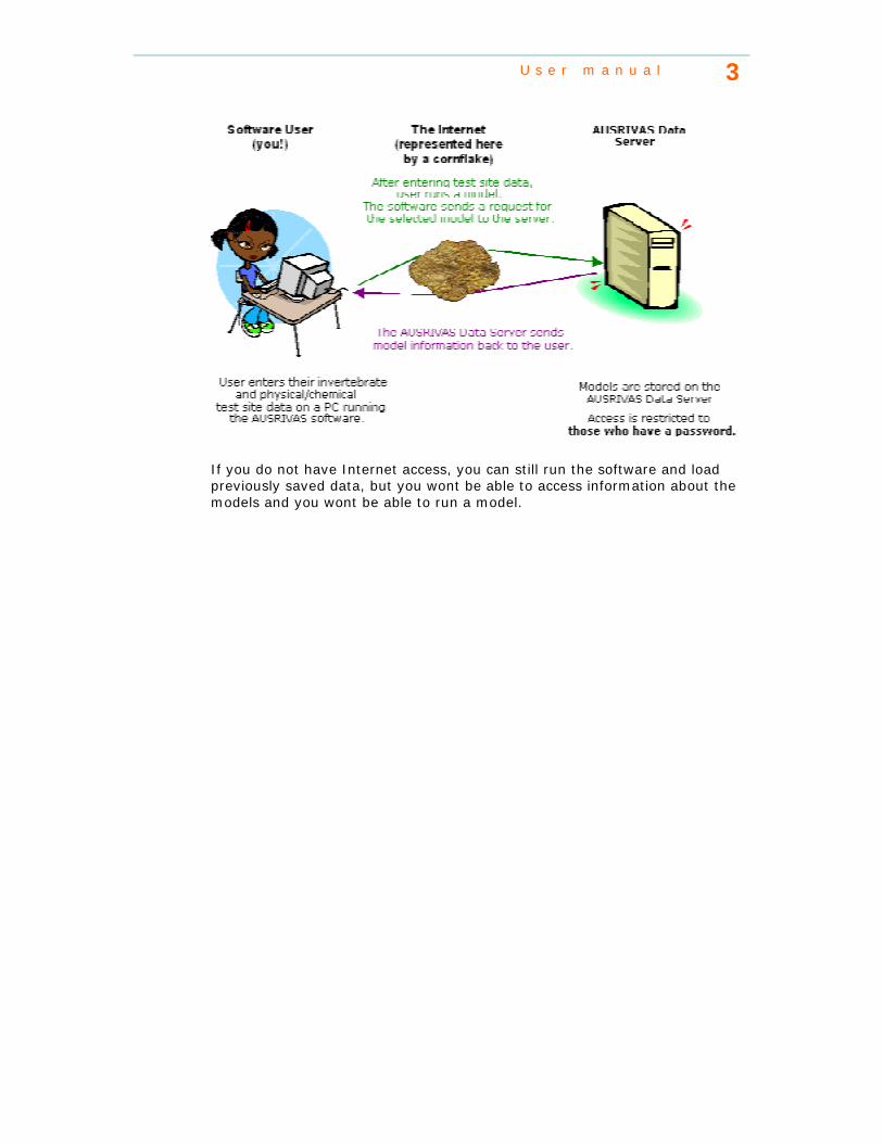
1.3 How the software uses the Internet
The AUSRIVAS Macroinvertebrate Predictive Modelling software requires Internet access in order to run a model. Model data is maintained at a central site and stored on a server at this site (currently at the CRCFE University of Canberra site). When an authorised user runs AUSRIVAS, the software connects to this central server to access the latest model information, and uses this to produce an assessment of the condition of a test site.
U s e r m a n u a l 3
If you do not have Internet access, you can still run the software and load previously saved data, but you wont be able to access information about the models and you wont be able to run a model.

4
Chapter 2: System requirements
2.1 Software requirements
2.1.1 Operating system1
! Microsoft © Windows NT/2000
! Microsoft © Windows XP
! Microsoft © Windows 98
! Microsoft © Windows 95 (with some modifications - see the MFC42.DLL error report)
2.1.2 Libraries
! Objective grid library OG80AS.DLL. This is distributed with AUSRIVAS.
! Microsoft © Windows library MFC42.DLL version 6.x or above. See the MFC42.DLL error report for further information.
! Microsoft © HTML Viewer, MSHTML.DLL. (Distributed with 'Windows') 1AUSRIVAS has not been tested with Windows ME. Feedback from users running AUSRIVAS under Windows ME would be appreciated.
2.2 Hardware requirements
2.2.1 Memory
The amount of memory required to run AUSRIVAS is made up of:
1. Memory used by the operating system and other running software.
2. Initial memory used by the AUSRIVAS program.
3. Memory used by AUSRIVAS in calculating the results.
The memory AUSRIVAS uses per site in calculating the results is proportional to the number of sites to be processed. So as more sites are processed, the amount of memory required per site increases.
For example, to process 2500 sites, AUSRIVAS uses 40KB of memory per site, whereas in order to process 4500 sites, AUSRIVAS requires 70KB of memory per site. This leads to a total of 100MB needed to process 2500 sites and 315MB for 4500 sites - more than three times as much for less than twice the number of sites.
It is important to note that the memory shown above is just for the calculating phase of running AUSRIVAS. When calculating memory requirements allow for additional memory for the operating system and initial memory use by the AUSRIVAS program.

U s e r m a n u a l 5
Windows 95 and 98
Windows 98 and 95 memory management appears to be faulty as only a fixed number of sites can be processed under these operating systems before the machine runs out of memory (users report figures such as 380 and 500 sites). This is independent of how much memory is in the machine (provided of course there is not too little memory).
Windows NT
Windows NT does not show the memory management problems seen in Win 95/98, so the calculations above can be used to determine how much memory you need to run AUSRIVAS. As an example, in calculating 2500 sites on my NT machine the memory usage was:
Usage (Windows NT) Memory Operating system + AUSRIVAS program 80 MB
AUSRIVAS calculations 100 MB
TOTAL 180 MB
It is recommend that the memory requirements are made up of actual physical memory rather than being made up of both real and virtual memory (memory temporarily stored to disk) otherwise processing will be slowed greatly.
2.2.2 Processor speed
Processor speed is not critical unless you plan to compute a large number of sites.
As an example, processing 2500 sites on a 550MHz PIII took over 30mins, while processing 4500 sites on the same machine took several hours.
2.3 Internet
There are two ways of running AUSRIVAS. You can work off-line, where the program does not access the Internet, or you can run AUSRIVAS over the Internet.
AUSRIVAS needs to access the Internet in order to
! Run a model;
! Access information about models, such as required predictor variables and model bands.
If you run the AUSRIVAS Macroinvertebrate Predictive Modelling Software without an Internet connection, you can:
! Load and view previously saved data.
Hint
You cannot run a model or access model information in off-line mode.

6
Further information
For more information on how AUSRIVAS uses the Internet, see the Section 1.3, ‘How the software uses the Internet’, in the introduction of this manual.
For information on how to set up AUSRIVAS to run over your Internet connection, see section 3.4, ‘Configuring the software for Internet access’.
Chapter 3: Getting started
3.1 Gaining access to the models
To access AUSRIVAS models from one of the suite of AUSRIVAS software packages, you need to have a username and password.
Hint
There is a charge for creating an AUSRIVAS username and password.
The cost is $80 (50% discount for non-profit organisations), which you will be billed for after your account is created.
3.1.1 To get an AUSRIVAS account
To apply for an AUSRIVAS account, please use the on-line form on the AUSRIVAS web site http://ausrivas.canberra.edu.au (select ‘Getting an AUSRIVAS password’ from the left-hand menu).
Your (completed) application is sent to your State or Territory NRHP contact for approval and then forwarded to the AUSRIVAS password administrator for creation of your account.
You will be notified of your AUSRIVAS username and password by e-mail, usually within two weeks. If you need your AUSRIVAS account sooner than this, please make sure your NRHP contact knows this.
If you cannot use the on-line form, please refer to the alternate method for obtaining an AUSRIVAS account detailed below.
If you can not use the on-line form
Alternative steps for obtaining an AUSRIVAS access code are detailed below:
1. Download or copy the AUSRIVAS Account Request Form and fill in the information requested (Fields 1 to 10 in the account request form).
2. Answer 'yes' to agreeing to abide by the conditions of use. The conditions of use are given on the account request form.
3. Send your completed AUSRIVAS account request form to your State or Territory NRHP contact.
U s e r m a n u a l 7
You will be notified of your AUSRIVAS username and password by e-mail, usually within two weeks. If you need your AUSRIVAS account sooner than this, please make sure your NRHP contact knows this.
Further information
If you need further information about obtaining AUSRIVAS software, please refer to the Software Users manual for the particular AUSRIVAS software package you are interested in.
Hint
If you use the alternative method for requesting a password (downloading & printing a form), make sure you send your account request to your State or Territory NRHP contact. The central body that administers AUSRIVAS accounts (the CRCFE at the University of Canberra) can only create accounts for requests approved by NRHP contacts.
Hint
If you use the alternative method for requesting a password (downloading & printing a form), make sure you read the Conditions of Use and answer 'yes' to agreeing to abide by the conditions of use (the last field in the account request form). Accounts cannot be created without this agreement.
3.1.2 Charges involved
There is a charge for getting an AUSRIVAS username and password.
This charge is calculated on a cost recovery basis, and covers the costs of creating your username and password only. The charge is $80, with a 50% discount for non-profit organisations, which you will be billed for after your account is created.
3.1.3 Conditions of use Please note that your AUSRIVAS username and password are confidential and are to be used by yourself only. New members of an organisation, including research staff and students, must obtain their own AUSRIVAS username and password.
Why can’t I give my password to someone else to use?
The restrictions on the transferral of AUSRIVAS accounts has come about for two reasons:
AUSRIVAS Training and accreditation
At the workshop for the AUSRIVAS Training and Accreditation project, State and Territory representatives, along with Environment Australia and CRCFE representatives, decided that passwords would be issued to individual users, rather than to groups of users, as had previously been the case. It was also decided that State and Territory NRHP representatives would authorise account requests from their relevant State or Territory.
AUSRIVAS mapping and reference site screening module
8
The AUSRIVAS Mapping and Reference Site Screening Module, due for release in 2003, makes use of 3rd party data - the 1:250k streamline data from AUSLIG. In order to allow use of this module without all users needing to have an AUSLIG license for the 1:250k streamline data, we reached an agreement with AUSLIG, which defines several conditions. One of these conditions is that access to the maps produced with the streamline data is password protected, where each authorised individual is known and has a non-transferable password.
3.1.4 I don't have an AUSRIVAS account. Can I still use the software? An AUSRIVAS username and password restricts access to AUSRIVAS models only. This means that you can make use of the software and utilise some of its functionality, as described below.
If you do not have an AUSRIVAS account, you can still:
! Download the AUSRIVAS software;
! Run the AUSRIVAS Macroinvertebrate Predictive Modelling software and: • Load and view previously saved data; • Find out which models are available; • Find out which predictor variables are used by a model; • Edit, print and save loaded data.
! Access the AUSRIVAS manuals (such as this one!) ! Request help. See Chapter 8 in this manual, or go to the AUSRIVAS web
site, http://ausrivas.canberra.edu.au and select ‘Macroinvertebrates’ then ‘Help’ from the left-hand menu (note that charges may apply).
However, you cannot run data through an AUSRIVAS model if you don’t have an AUSRIVAS account.
3.2 Obtaining the software The AUSRIVAS Macroinvertebrate Predictive Modelling software is available via download from the AUSRIVAS website. Go to http://ausrivas.canberra.edu.au/Bioassessment/Macroinvertebrates/ and select 'Get the predictive modelling software' from the left-hand menu.
3.3 Installing the predictive modelling software Once you have obtained a copy of the AUSRIVAS software, you can begin to install it on your computer. The following steps take you through the process of installing AUSRIVAS.
3.3.1 Safeguard older program versions Before you start to install the new version of AUSRIVAS, you should safeguard your old version if you have one. You could do this by:
i. Moving it to an out of the way folder such as
c:\Program Files\Ausrivas_1-3.
ii. Renaming it, say from ausrivas.exe to ausrivas_1-3.exe.
U s e r m a n u a l 9
3.3.2 Create a folder for the software If you haven't done so already, create the folder you want to install AUSRIVAS in and move the downloaded file, Ausrivas_2-2.exe, to this folder. For the rest of this guide, I'll assume you want to put AUSRIVAS into the folder
c:\Program Files\Ausrivas\.
3.3.3 Extract the AUSRIVAS program The file you have downloaded, Ausrivas_2-2.exe, is a compressed file. To uncompress it you double-click on the filename Ausrivas_2-2.exe in Windows Explorer or My Computer
This will create two files, ausrivas.exe and og80as.dll in the folder you created in Step 2.
Hint
If you cant see the file og80as.dll, start Windows Explorer and choose 'View all files' from the 'View/Options' menu.
3.3.4 Set up library files You now need to copy og80as.dll to the correct location on your hard disk.
i. Windows 95/98 users should copy the file to the
c:\Windows\System folder.
ii. Windows NT users should copy the file to the
c:\WinNT\System32 folder.
iii. Windows 2000 users should consult their systems administrator to find out where to put this DLL.
3.3.5 More hints
Hint
If you are running an oldish version of Windows 95, or if you get an error similar to:
The og80as.dll is linked to missing export mfc42.dll:6605
refer to the Section on DLL Errors under MFC42.DLL Error in the ‘Troubleshooting guide’ (Chapter 6).
Hint
For information on how to use the AUSRIVAS program, refer to the AUSRIVAS Predictive Modelling manual at:
http://ausrivas.canberra.edu.au/Bioassessment/Macroinvertebrates/Man/Pred/.
10
Hint
When all else fails .... first talk to your systems administrator - most problems fall under her or his domain. If your systems administrator believes the problem to originate with the AUSRIVAS program, refer to our help page in Chapter 8 for the name of someone to contact at the CRCFE.
3.4 Configuring the software for Internet access
3.4.1 Running AUSRIVAS with or without Internet access.
There are two ways of running AUSRIVAS (called "run options"). You can work off-line, where the program does not access the Internet, or you can run AUSRIVAS over the Internet (in on-line mode). These run options are explained below.
Running AUSRIVAS over the Internet (On-line mode).
AUSRIVAS needs to access the Internet in order to
! Run a model;
! Access information about models, such as required predictor variables and model bands.
You can access the Internet in two ways, either directly or through a proxy server. To find out which Internet access method you need to use, contact your local systems administrator. If you do access the Internet through a proxy server, you will need to give AUSRIVAS two pieces of information about your proxy server:
1. The name of your proxy server
2. The port your proxy server runs on.
More information about these is given in the section below on Proxy Server settings.
If you access the Internet through a proxy server, you will need to know if your proxy server requires authentication. You can get this information from your systems administrator. If your proxy server does require authentication, you will need to know:
1. Your Internet username;
2. Your Internet password.
More information about these is given in the section below on Proxy Authentication.
Running AUSRIVAS off-line.
Alternately, you can choose to work off-line. In off-line mode, you can load and view previously saved data.
U s e r m a n u a l 11
Hint
You cannot run a model or access model information in off-line mode.
3.4.2 Selecting your run options
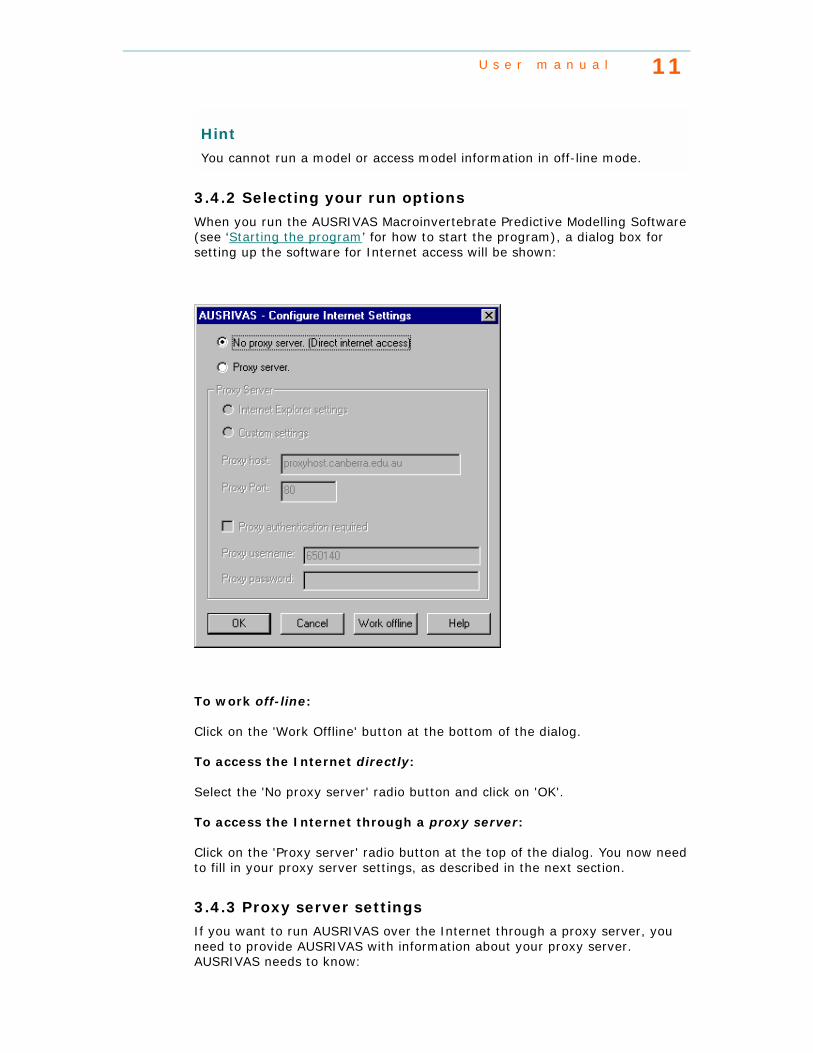
When you run the AUSRIVAS Macroinvertebrate Predictive Modelling Software (see ‘Starting the program’ for how to start the program), a dialog box for setting up the software for Internet access will be shown:
To work off-line:
Click on the 'Work Offline' button at the bottom of the dialog.
To access the Internet directly:
Select the 'No proxy server' radio button and click on 'OK'.
To access the Internet through a proxy server:
Click on the 'Proxy server' radio button at the top of the dialog. You now need to fill in your proxy server settings, as described in the next section.
3.4.3 Proxy server settings
If you want to run AUSRIVAS over the Internet through a proxy server, you need to provide AUSRIVAS with information about your proxy server. AUSRIVAS needs to know:
12
! The name of your proxy server.
! The port your proxy server runs on.
The name of your proxy server is made up of a machine name followed by your Internet domain. For example, the proxy server at the University of Canberra is called proxyhost.canberra.edu.au.
The port number your proxy server runs on is an integer. Many proxy servers run on port 80.
There are two ways you can provide AUSRIVAS with this information:
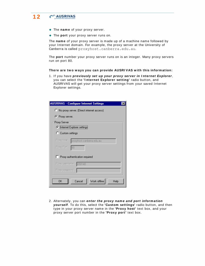
1. If you have previously set up your proxy server in Internet Explorer, you can select the 'Internet Explorer setting' radio button, and AUSRIVAS will get your proxy server settings from your saved Internet Explorer settings.
2. Alternately, you can enter the proxy name and port information yourself. To do this, select the 'Custom settings' radio button, and then type in your proxy server name in the 'Proxy host' text box, and your proxy server port number in the 'Proxy port' text box.
U s e r m a n u a l 13
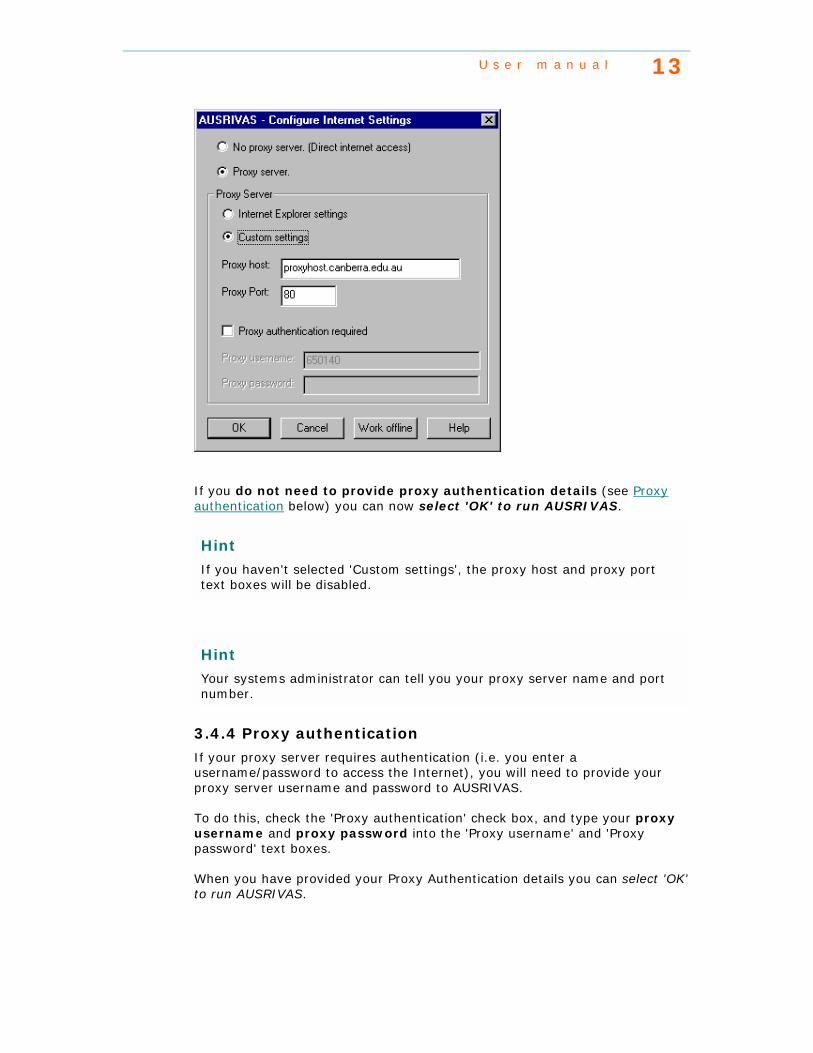
If you do not need to provide proxy authentication details (see Proxy authentication below) you can now select 'OK' to run AUSRIVAS.
Hint
If you haven't selected 'Custom settings', the proxy host and proxy port text boxes will be disabled.
Hint
Your systems administrator can tell you your proxy server name and port number.
3.4.4 Proxy authentication
If your proxy server requires authentication (i.e. you enter a username/password to access the Internet), you will need to provide your proxy server username and password to AUSRIVAS.
To do this, check the 'Proxy authentication' check box, and type your proxy username and proxy password into the 'Proxy username' and 'Proxy password' text boxes.
When you have provided your Proxy Authentication details you can select 'OK' to run AUSRIVAS.

14
Hint
If you have not checked the 'Proxy authentication' check box, the 'Proxy username' and 'Proxy password' text boxes will be disabled.
Hint
If you do not know what your proxy username and password are, or if you do not know if you need one, ask your local Systems Administrator.
3.4.5 Saving settings
When you click on 'OK', AUSRIVAS will save all of your proxy settings except your proxy password, for use the next time you run AUSRIVAS.
3.4.6 Altering your Internet settings
You can change your Internet settings while you are running AUSRIVAS, by opening the 'Internet Settings' dialog from the 'Options/Proxy server settings ...' menu. You will also always be shown the 'Internet Settings' dialog each time you run the program in case you need to change your options.

U s e r m a n u a l 15
Hint
Once you have selected to run in either off-line or on-line mode, you cannot change this while you are running the program. To go from off-line to on-line mode or vice-versa, you will need to quit the AUSRIVAS program and restart.

16
Chapter 4: Using the AUSRIVAS software
4.1 Starting the AUSRIVAS program
By double-clicking on the AUSRIVAS icon, (either in Explorer on the Desktop if you have set up a shortcut) the AUSRIVAS program will open. It has a series of labelled overlying sheets with menus and a toolbar across the top of the page and a status indicator at the base.
The first sheet is for the entry of invertebrate data, the second sheet for entry of habitat data. The remaining sheets will contain various outputs from the model once it has been run. The complete list of data sheets is:
1. Bug Data - This is where you enter your invertebrate data.
2. Phys/Chem Data - This is where you enter your predictor variables.
3. Group Probabilities - Shows group probabilities after a model has been run.
4. Taxon Probabilities - Shows taxon probabilities after a model has been run.
5. Predicted/Collected - Shows output statistics after a model has been run.
6. Unused Bugs - The taxa that were not used when the model was run are moved to this sheet.
The toolbar includes some standard Microsoft Windows menu items along with a few new ones for importing and exporting text format data.
4.2 Preparing data
AUSRIVAS requires the use of specific codes for the invertebrate taxa and habitat variables. Family level taxonomic codes for macroinvertebrate taxa are available from the AUSRIVAS website at http://ausrivas.canberra.edu.au/Bioassessment/Macroinvertebrates/ (select 'Taxonomy' from the left hand menu) listed in alphabetical order by both codes and family name. To combine data for entry in to a combined-season
U s e r m a n u a l 17
model the habitat data should be averaged and the invertebrate data summed for the same site sampled in both spring and autumn. Macroinvertebrate data may be entered as either totals or as presence/absence data, however, AUSRIVAS will convert all invertebrate data to presence absence form for analysis when a model is run.
Which predictor variables to I need?
The predictor variables required may be different for each model. A list of the habitat variable codes required for each model can be obtained through the AUSRIVAS software, as described below.
Hint
You must be running in on-line mode to access the list of habitat variables.
Hint
You do not need to have a password to view the list of habitat variables.
Viewing required predictor variables
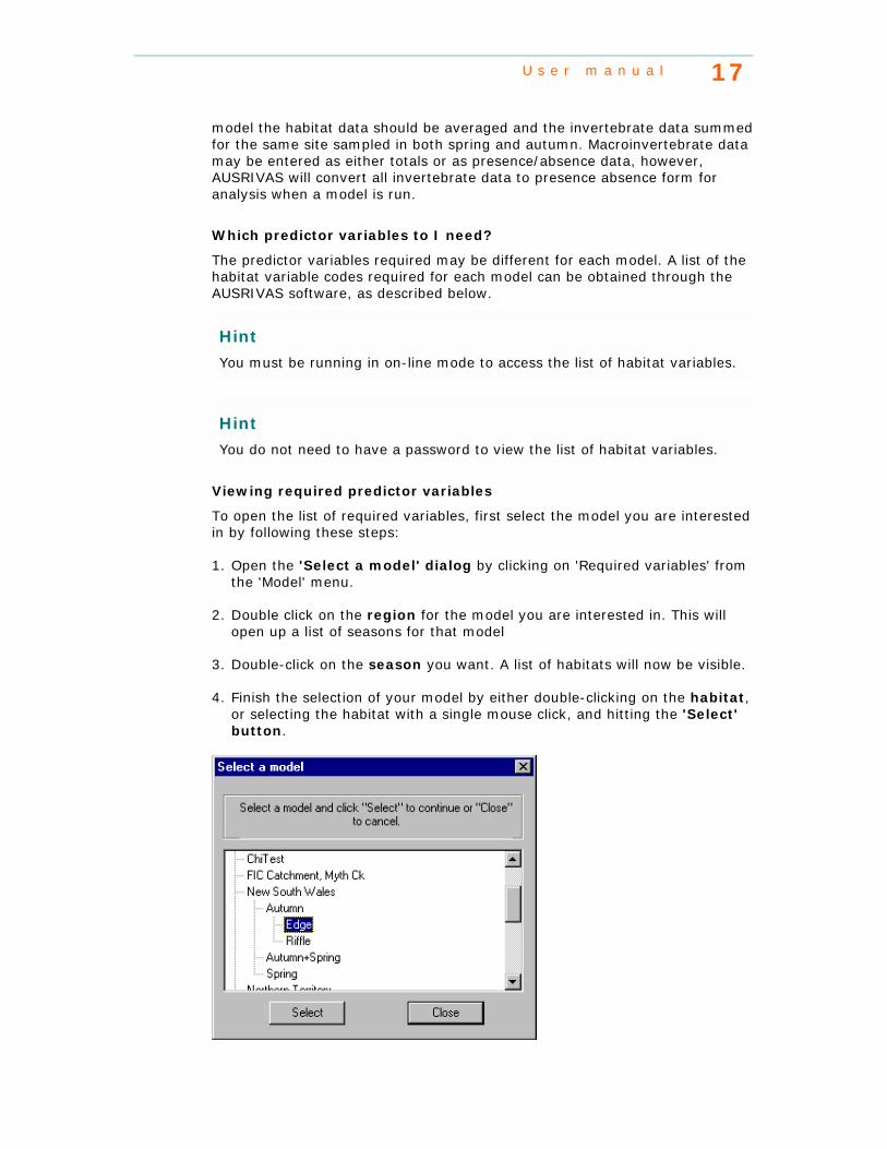
To open the list of required variables, first select the model you are interested in by following these steps:
1. Open the 'Select a model' dialog by clicking on 'Required variables' from the 'Model' menu.
2. Double click on the region for the model you are interested in. This will open up a list of seasons for that model
3. Double-click on the season you want. A list of habitats will now be visible.
4. Finish the selection of your model by either double-clicking on the habitat, or selecting the habitat with a single mouse click, and hitting the 'Select' button.
18
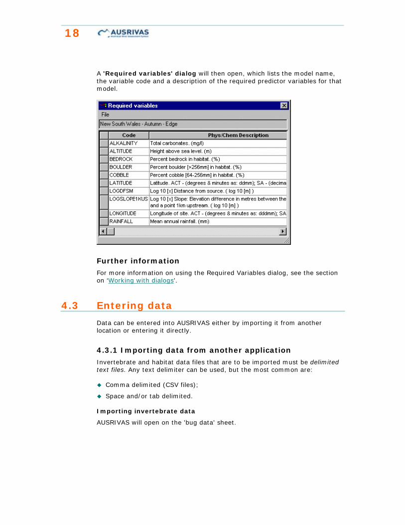
A 'Required variables' dialog will then open, which lists the model name, the variable code and a description of the required predictor variables for that model.
Further information
For more information on using the Required Variables dialog, see the section on ‘Working with dialogs’.
4.3 Entering data
Data can be entered into AUSRIVAS either by importing it from another location or entering it directly.
4.3.1 Importing data from another application
Invertebrate and habitat data files that are to be imported must be delimited text files. Any text delimiter can be used, but the most common are:
! Comma delimited (CSV files);
! Space and/or tab delimited.
Importing invertebrate data
AUSRIVAS will open on the 'bug data' sheet.

U s e r m a n u a l 19
To import your invertebrate data file open the 'File' menu and select 'Import'
or click on the import button on the toolbar . A box listing possible file formats and attributes will appear. Note that your data file must contain the site codes and taxa codes. If the first data item in each of the rows in your file is the site code, select the 'with Row Headers' option, and the site codes will be used row headings in AUSRIVAS. The same applied to column headings. If the first row in your data file contains taxon codes, select the 'with Column Headings' options and the taxon codes will be imported into your AUSRIVAS spreadsheet.
Now you need to let AUSRIVAS know about the format of your file. As discussed above, your file must be in a text delimited format, so you just need to specify the delimiter used in your file. In the diagram above, the delimiter is specified as "Space & Tab Delimiting". This means that the gaps between each data item in a row of data are made up of spaces and/or tabs. You can separate your data with other delimiters if you wish. The diagram below shows how to specify that your data is a CSV file (separated with commas). Note that the option 'Other' has been selected for delimiter type, and the delimiter itself (a comma) has been entered into the text box beside the 'Other' option.
When you have specified the type of delimiter in the text file you wish to import, click 'OK'. A directory box will open allowing you to browse and select the file to be imported.
20
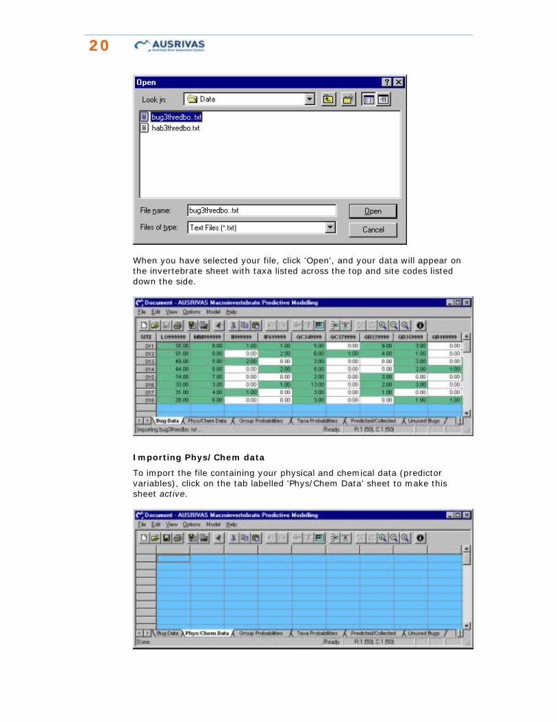
When you have selected your file, click 'Open', and your data will appear on the invertebrate sheet with taxa listed across the top and site codes listed down the side.
Importing Phys/Chem data
To import the file containing your physical and chemical data (predictor variables), click on the tab labelled 'Phys/Chem Data' sheet to make this sheet active.

U s e r m a n u a l 21
The procedure is now the same as used for the invertebrate data (but with predictor variable codes rather than taxa codes).
Once the data is entered, both spreadsheets should be trimmed to ensure no
blank rows or columns, using the 'delete blank rows and columns' icon .
Hint
The 'trimming' procedure will also indicate any extraneous data in rows and columns, which will require deletion.
4.3.2 Entering data directly into AUSRIVAS
To enter the invertebrate codes and site codes into the 'bug data' sheet, double click on the desired header box. A cursor will appear allowing the headers to be entered. To enter the data simply click on the desired cell. If at a later date you wish to modify an entry, a single click will allow replacing an entry while a double click will allow the entry to be modified. Once the invertebrate data has been entered click on the tab at the bottom of the screen for the phys/chem sheet. A blank sheet will open to enter the physical and chemical variables that are required to run the model. Again, once the data is entered, both spreadsheets should be trimmed to ensure no blank
rows or columns, using the 'delete blank rows and columns' icon .
Hint
Before proceeding to run the AUSRIVAS model you should save the AUSRIVAS file with your input data. If errors are encountered from this point on you can easily re-open the saved file and correct any errors, which may save you the time of importing the data again.
4.3.3 Checking your input data for errors
Invertebrate data
It is important that there are no blank cells, as a site assessment cannot be produced for sites with blank cells in the invertebrate data. AUSRIVAS will highlight any cells with blank data as shown below. This screen shot shows how a blank cell is highlighted in blue.
AUSRIVAS will also warn you when it does not recognise a taxon code. The causes of this will be either:
! The taxon code is incorrect. In this case check the list of valid invertebrate codes. (NOTE: TAXA CODES AND HABITAT VARIABLE NAMES ARE CASE SENSITIVE).
22
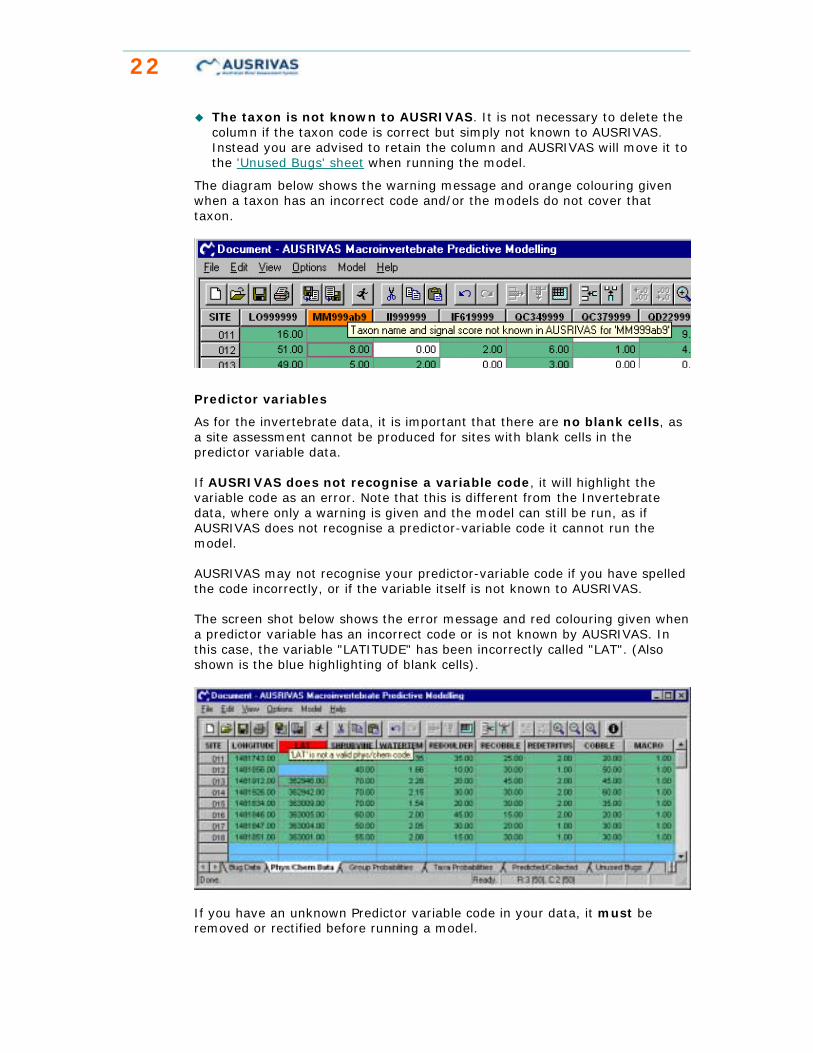
! The taxon is not known to AUSRIVAS. It is not necessary to delete the column if the taxon code is correct but simply not known to AUSRIVAS. Instead you are advised to retain the column and AUSRIVAS will move it to the 'Unused Bugs' sheet when running the model.
The diagram below shows the warning message and orange colouring given when a taxon has an incorrect code and/or the models do not cover that taxon.
Predictor variables
As for the invertebrate data, it is important that there are no blank cells, as a site assessment cannot be produced for sites with blank cells in the predictor variable data.
If AUSRIVAS does not recognise a variable code, it will highlight the variable code as an error. Note that this is different from the Invertebrate data, where only a warning is given and the model can still be run, as if AUSRIVAS does not recognise a predictor-variable code it cannot run the model.
AUSRIVAS may not recognise your predictor-variable code if you have spelled the code incorrectly, or if the variable itself is not known to AUSRIVAS.
The screen shot below shows the error message and red colouring given when a predictor variable has an incorrect code or is not known by AUSRIVAS. In this case, the variable "LATITUDE" has been incorrectly called "LAT". (Also shown is the blue highlighting of blank cells).
If you have an unknown Predictor variable code in your data, it must be removed or rectified before running a model.

U s e r m a n u a l 23
4.3.4 Removing/editing data
If you want to change your data because of an error or warning, you can do so by either:
! Editing and re-importing the original data file, or
! entering the correct values directly into the invertebrate sheet.
Deleting a data column
To delete a data column, click in the header box of that column and the column will be highlighted. Next click on the edit menu and select remove column and the selected column will be deleted.
Care should be taken when removing taxa that those taxa that are required by the model are not deleted. If you do omit taxa that are required by the model, a dialog box that appears after running a model will identify any missing taxa and habitat variables.
4.4 Choosing a model
4.4.1 Which model do I use?
For each state/territory a minimum choice of 6 models is available; 2 habitats and 2 seasons, plus a combined-seasons model for each habitat. Where and how the test site data were collected will determine the model required to provide a site assessment. Test data can only be run though a model created for the same state, territory or region your data has been collected in, and it must have been collected using the same methods (see the section on ‘Sampling manuals’ on the Macroinvertebrates section of the AUSRIVAS website), as this will affect the results obtained. For example, a test site sampled in the ACT according to territory protocols could not be assessed using a NSW model, as macroinvertebrate sample processing for ACT models is done in a laboratory, whereas NSW models use a field live-pick protocol. Habitat predictor variables are also likely to be measured differently in different states and territories, which will also affect the results obtained. Similarly, the habitat sampled will affect the biota collected, therefore a riffle model can only be used to assess data collected in a riffle habitat in the same region, sampled in the same way as the data used to create the model. When selecting a season, use the seasonal model closest to the season your test site was sampled in (check the appropriate state/territory sampling manual for definition of sampling seasons). However, if both an autumn and spring sample of a test site are available, it is preferable to combine the data and choose the combined (autumn+spring) season model, ensuring the taxa list for the test site is maximised.
4.4.2 Selecting and running a model in the program
To select and run a model once data entry is complete, click on the ‘run model’ menu.

24
A 'wizard' will now appear, that lets you (in order):
1. Enter your AUSRIVAS username and password;
2. Select the region your data was sampled in;
3. Select the season your data was sampled;
4. Select the habitat your data was sampled from.
To run a model using this wizard, first enter your AUSRIVAS username and password and click ‘next’.
Then select the state, territory or region your test sites were sampled in and click ‘next’.
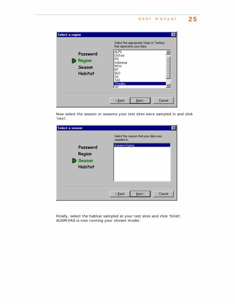
U s e r m a n u a l 25
Now select the season or seasons your test sites were sampled in and click ‘next’.
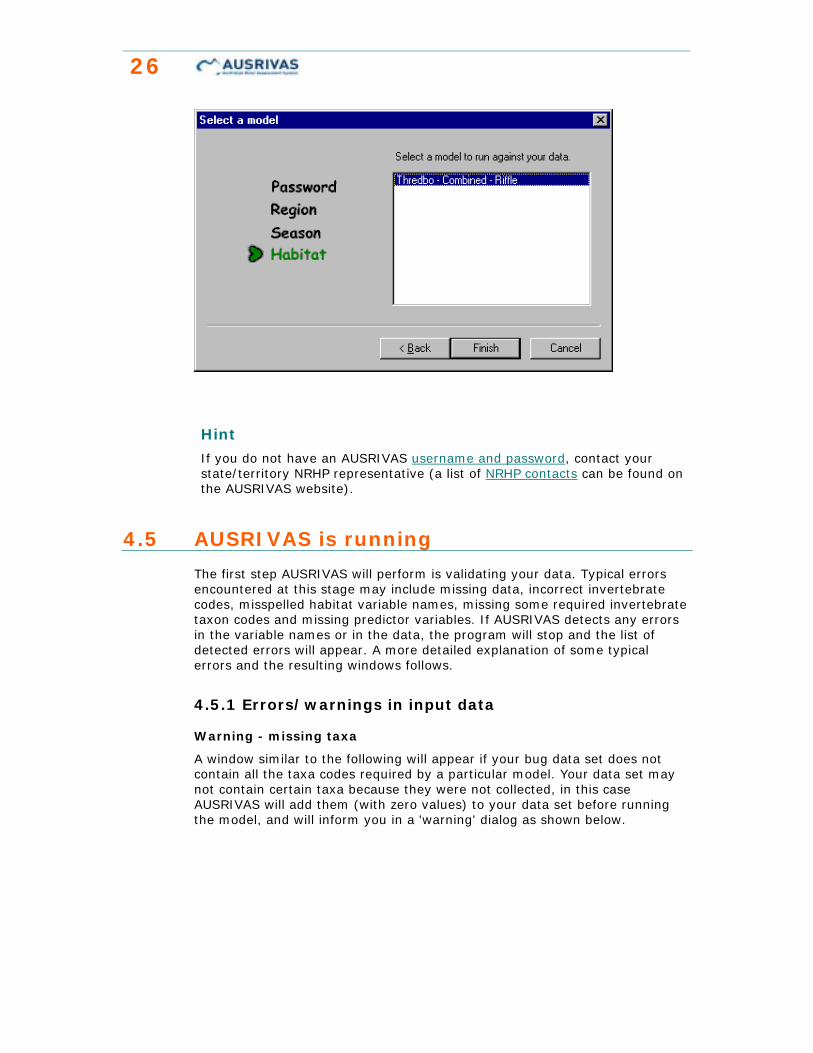
Finally, select the habitat sampled at your test sites and click ‘finish’. AUSRIVAS is now running your chosen model.
26
Hint
If you do not have an AUSRIVAS username and password, contact your state/territory NRHP representative (a list of NRHP contacts can be found on the AUSRIVAS website).
4.5 AUSRIVAS is running
The first step AUSRIVAS will perform is validating your data. Typical errors encountered at this stage may include missing data, incorrect invertebrate codes, misspelled habitat variable names, missing some required invertebrate taxon codes and missing predictor variables. If AUSRIVAS detects any errors in the variable names or in the data, the program will stop and the list of detected errors will appear. A more detailed explanation of some typical errors and the resulting windows follows.
4.5.1 Errors/warnings in input data
Warning - missing taxa
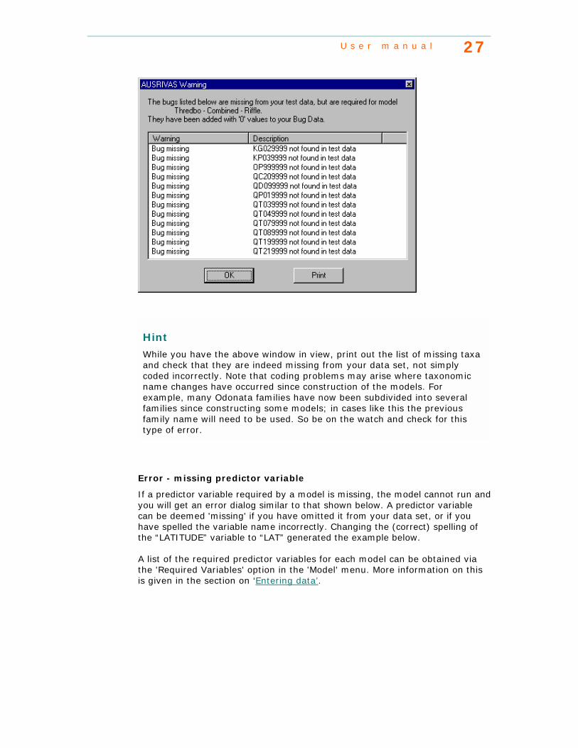
A window similar to the following will appear if your bug data set does not contain all the taxa codes required by a particular model. Your data set may not contain certain taxa because they were not collected, in this case AUSRIVAS will add them (with zero values) to your data set before running the model, and will inform you in a 'warning' dialog as shown below.
U s e r m a n u a l 27
Hint
While you have the above window in view, print out the list of missing taxa and check that they are indeed missing from your data set, not simply coded incorrectly. Note that coding problems may arise where taxonomic name changes have occurred since construction of the models. For example, many Odonata families have now been subdivided into several families since constructing some models; in cases like this the previous family name will need to be used. So be on the watch and check for this type of error.
Error - missing predictor variable
If a predictor variable required by a model is missing, the model cannot run and you will get an error dialog similar to that shown below. A predictor variable can be deemed 'missing' if you have omitted it from your data set, or if you have spelled the variable name incorrectly. Changing the (correct) spelling of the “LATITUDE” variable to “LAT” generated the example below.
A list of the required predictor variables for each model can be obtained via the 'Required Variables' option in the 'Model' menu. More information on this is given in the section on ‘Entering data’.

28
Error - site mismatch
If the site codes listed in the Bug Data file do not match exactly those in the Phys/Chem data file a window similar to the following will appear explaining the error.
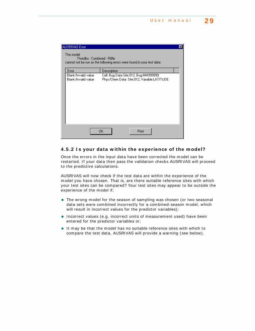
Error - blank data cells
It is important that there are no blank cells, as a site assessment cannot be produced for sites with blank cells in either the invertebrate data or the predictor variables. AUSRIVAS highlights any cells with blank data in the input data sheets in blue. If data is not inserted in these blank cells before a model is run, you will get an error as shown below. The error description tells you in which sheet ("Bug Data") and which row (Site 012) and column (MM999999) the blank/invalid cell occurs.
U s e r m a n u a l 29
4.5.2 Is your data within the experience of the model?
Once the errors in the input data have been corrected the model can be restarted. If your data then pass the validation checks AUSRIVAS will proceed to the predictive calculations.
AUSRIVAS will now check if the test data are within the experience of the model you have chosen. That is, are there suitable reference sites with which your test sites can be compared? Your test sites may appear to be outside the experience of the model if;
! The wrong model for the season of sampling was chosen (or two seasonal data sets were combined incorrectly for a combined-season model, which will result in incorrect values for the predictor variables);
! Incorrect values (e.g. incorrect units of measurement used) have been entered for the predictor variables or;
! It may be that the model has no suitable reference sites with which to compare the test data, AUSRIVAS will provide a warning (see below).
30
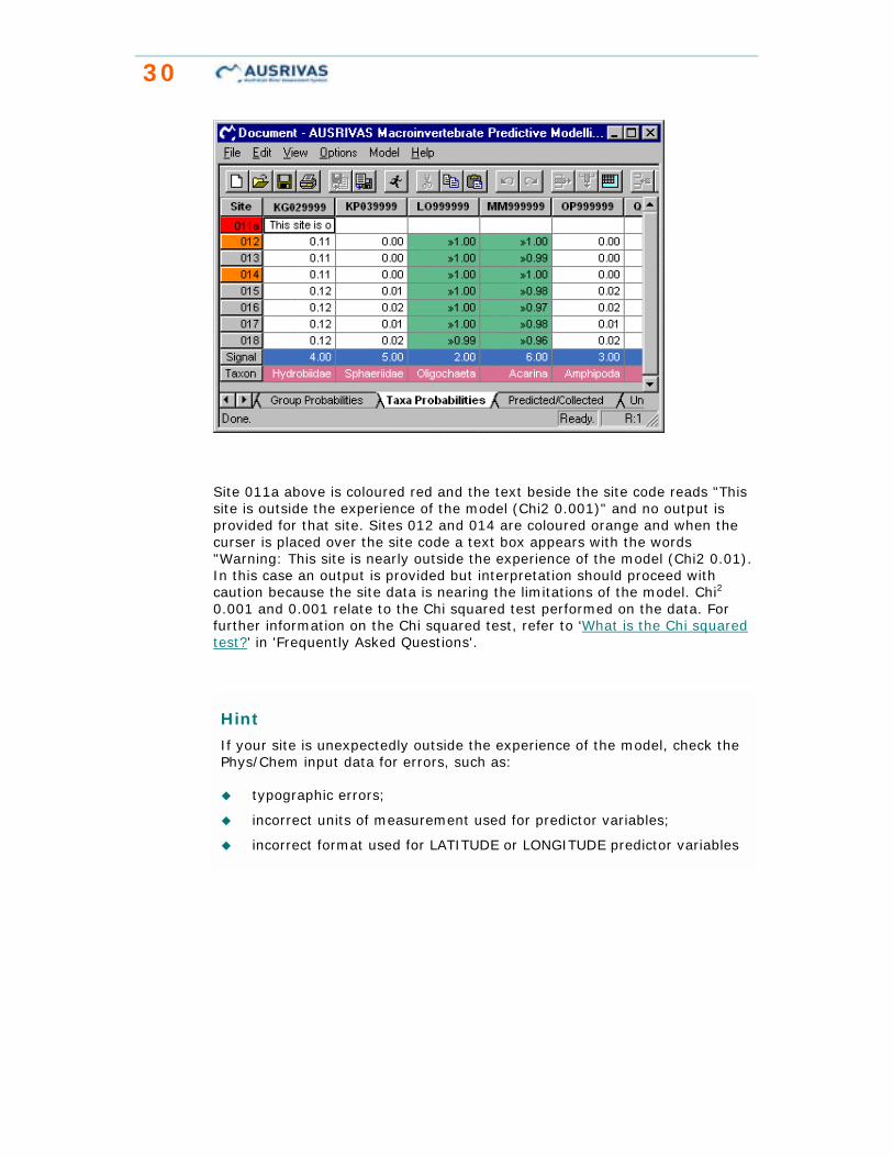
Site 011a above is coloured red and the text beside the site code reads "This site is outside the experience of the model (Chi2 0.001)" and no output is provided for that site. Sites 012 and 014 are coloured orange and when the curser is placed over the site code a text box appears with the words "Warning: This site is nearly outside the experience of the model (Chi2 0.01). In this case an output is provided but interpretation should proceed with caution because the site data is nearing the limitations of the model. Chi2 0.001 and 0.001 relate to the Chi squared test performed on the data. For further information on the Chi squared test, refer to ‘What is the Chi squared test?’ in 'Frequently Asked Questions'.
Hint
If your site is unexpectedly outside the experience of the model, check the Phys/Chem input data for errors, such as:
! typographic errors;
! incorrect units of measurement used for predictor variables;
! incorrect format used for LATITUDE or LONGITUDE predictor variables
U s e r m a n u a l 31
Hint
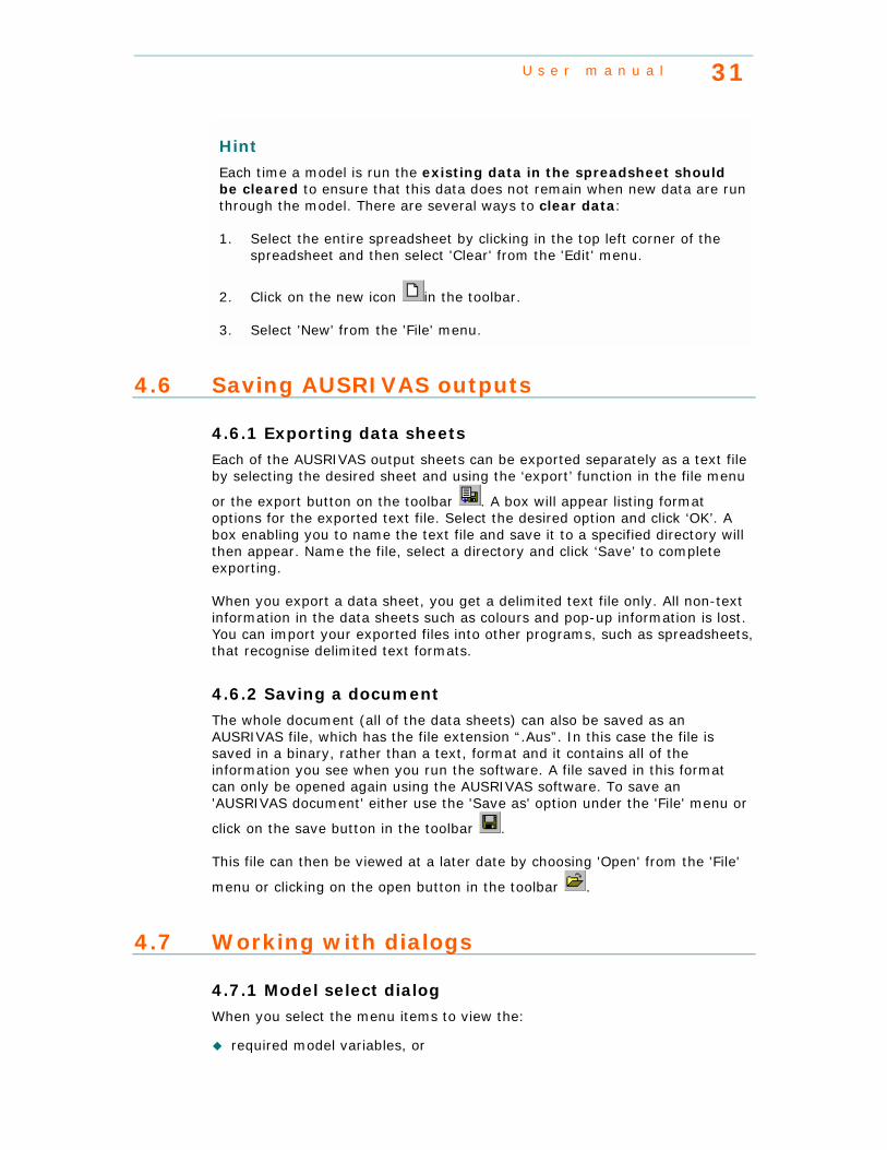
Each time a model is run the existing data in the spreadsheet should be cleared to ensure that this data does not remain when new data are run through the model. There are several ways to clear data:
1. Select the entire spreadsheet by clicking in the top left corner of the spreadsheet and then select 'Clear' from the 'Edit' menu.
2. Click on the new icon in the toolbar.
3. Select 'New' from the 'File' menu.
4.6 Saving AUSRIVAS outputs
4.6.1 Exporting data sheets
Each of the AUSRIVAS output sheets can be exported separately as a text file by selecting the desired sheet and using the ‘export’ function in the file menu
or the export button on the toolbar . A box will appear listing format options for the exported text file. Select the desired option and click ‘OK’. A box enabling you to name the text file and save it to a specified directory will then appear. Name the file, select a directory and click ‘Save’ to complete exporting.
When you export a data sheet, you get a delimited text file only. All non-text information in the data sheets such as colours and pop-up information is lost. You can import your exported files into other programs, such as spreadsheets, that recognise delimited text formats.
4.6.2 Saving a document
The whole document (all of the data sheets) can also be saved as an AUSRIVAS file, which has the file extension “.Aus”. In this case the file is saved in a binary, rather than a text, format and it contains all of the information you see when you run the software. A file saved in this format can only be opened again using the AUSRIVAS software. To save an 'AUSRIVAS document' either use the 'Save as' option under the 'File' menu or
click on the save button in the toolbar .
This file can then be viewed at a later date by choosing 'Open' from the 'File'
menu or clicking on the open button in the toolbar .
4.7 Working with dialogs
4.7.1 Model select dialog
When you select the menu items to view the:
! required model variables, or
32
! model bandwidths
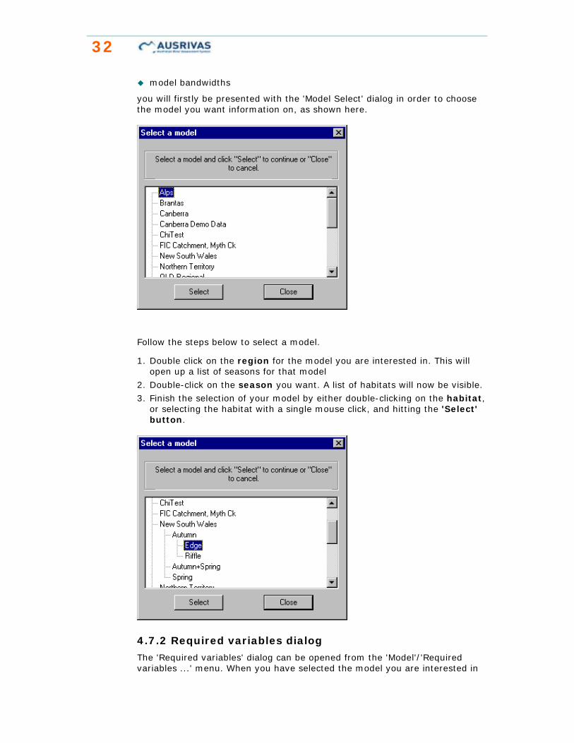
you will firstly be presented with the 'Model Select' dialog in order to choose the model you want information on, as shown here.
Follow the steps below to select a model.
1. Double click on the region for the model you are interested in. This will open up a list of seasons for that model
2. Double-click on the season you want. A list of habitats will now be visible. 3. Finish the selection of your model by either double-clicking on the habitat,
or selecting the habitat with a single mouse click, and hitting the 'Select' button.
4.7.2 Required variables dialog
The 'Required variables' dialog can be opened from the 'Model'/'Required variables ...' menu. When you have selected the model you are interested in

U s e r m a n u a l 33
(see Select model dialog above), the 'Required variables' dialog will open for the model you have chosen. This dialog lists the
! Model name; ! Variable codes for that models required variables;
! Description of the variables.
Viewing data
The 'Required variables' dialog is scrollable and resizable, so you can either scroll to view items that do not fit in the dialog, or you can make the dialog bigger.
Printing
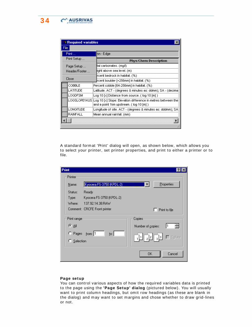
You can print data shown in the 'Required variables' dialog. Select 'Print' from the 'File' menu:
34
A standard format 'Print' dialog will open, as shown below, which allows you to select your printer, set printer properties, and print to either a printer or to file.
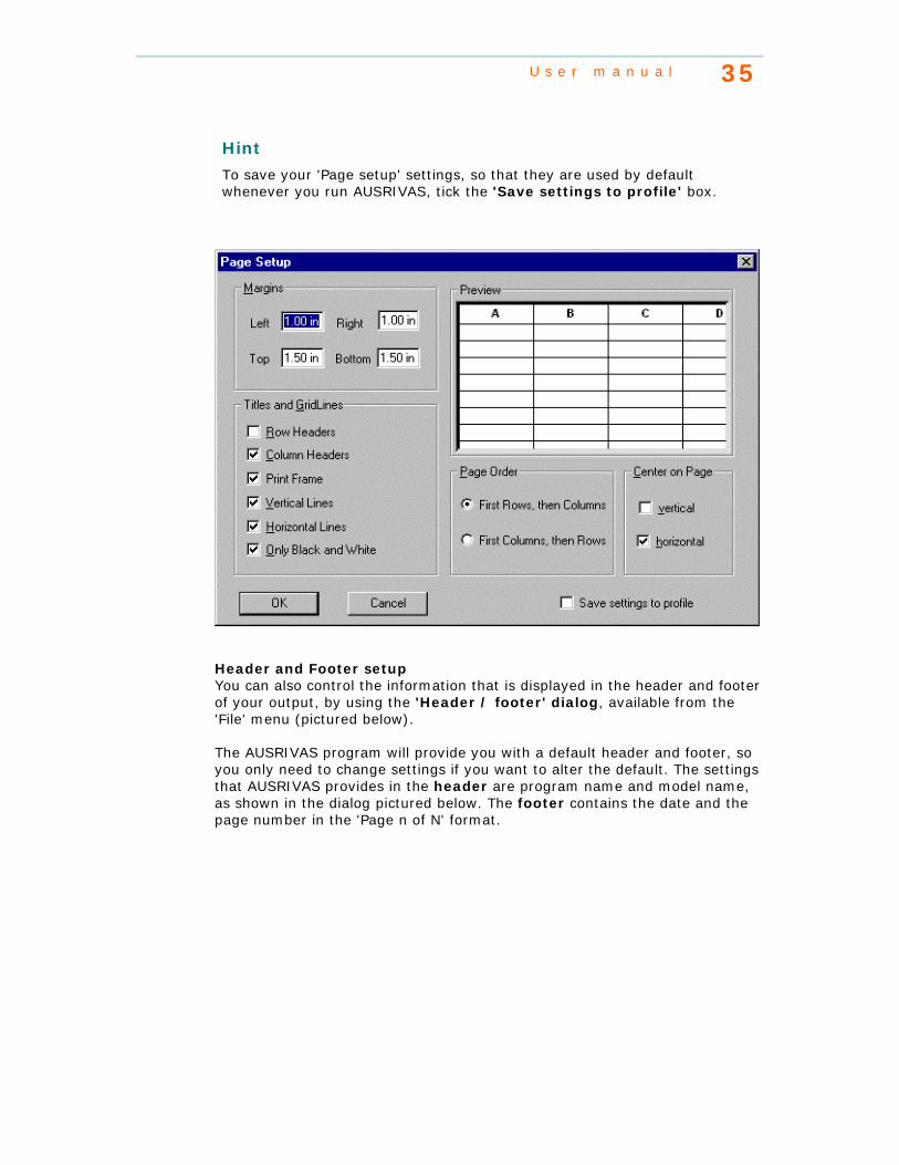
Page setup You can control various aspects of how the required variables data is printed to the page using the 'Page Setup' dialog (pictured below). You will usually want to print column headings, but omit row headings (as these are blank in the dialog) and may want to set margins and chose whether to draw grid-lines or not.
U s e r m a n u a l 35
Hint
To save your 'Page setup' settings, so that they are used by default whenever you run AUSRIVAS, tick the 'Save settings to profile' box.
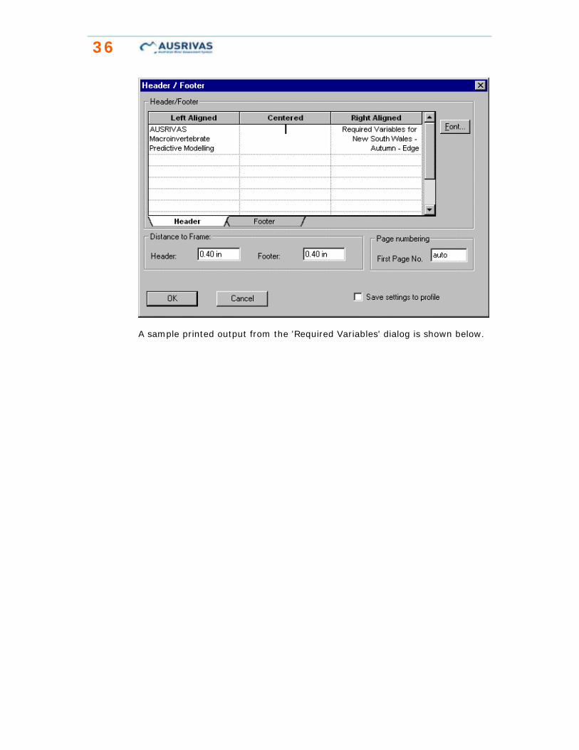
Header and Footer setup You can also control the information that is displayed in the header and footer of your output, by using the 'Header / footer' dialog, available from the 'File' menu (pictured below).
The AUSRIVAS program will provide you with a default header and footer, so you only need to change settings if you want to alter the default. The settings that AUSRIVAS provides in the header are program name and model name, as shown in the dialog pictured below. The footer contains the date and the page number in the 'Page n of N' format.
36
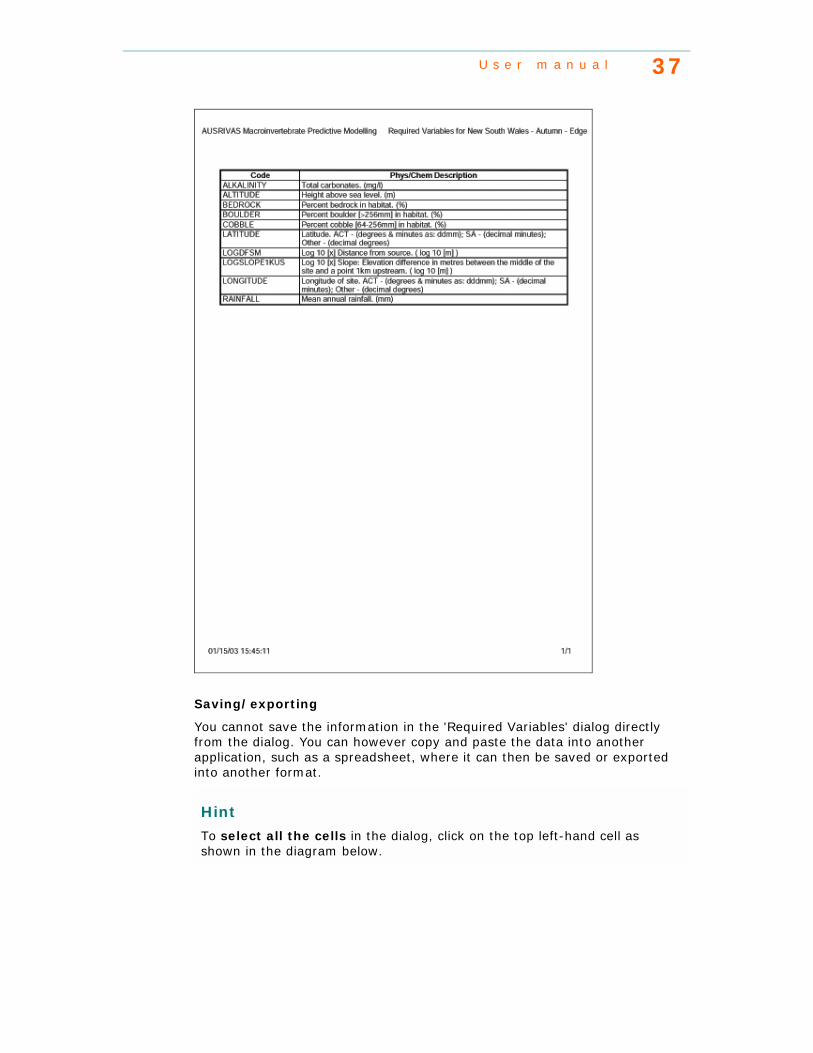
A sample printed output from the 'Required Variables' dialog is shown below.
U s e r m a n u a l 37
Saving/exporting
You cannot save the information in the 'Required Variables' dialog directly from the dialog. You can however copy and paste the data into another application, such as a spreadsheet, where it can then be saved or exported into another format.
Hint
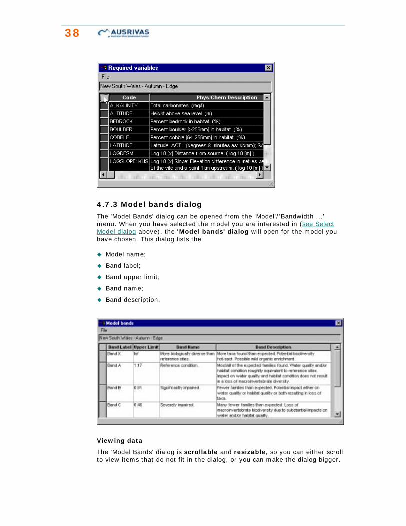
To select all the cells in the dialog, click on the top left-hand cell as shown in the diagram below.
38
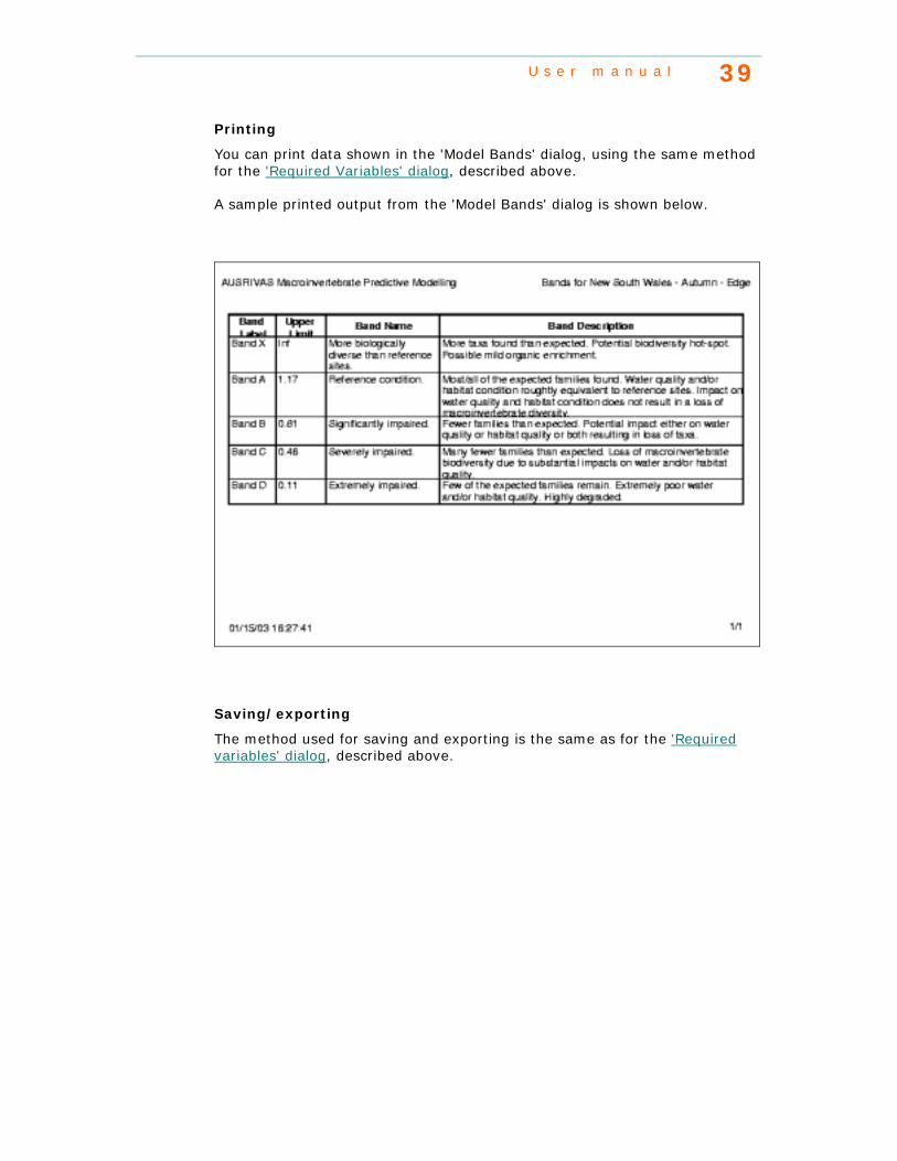
4.7.3 Model bands dialog
The 'Model Bands' dialog can be opened from the 'Model'/'Bandwidth ...' menu. When you have selected the model you are interested in (see Select Model dialog above), the 'Model bands' dialog will open for the model you have chosen. This dialog lists the
! Model name;
! Band label;
! Band upper limit;
! Band name;
! Band description.
Viewing data
The 'Model Bands' dialog is scrollable and resizable, so you can either scroll to view items that do not fit in the dialog, or you can make the dialog bigger.
U s e r m a n u a l 39
Printing
You can print data shown in the 'Model Bands' dialog, using the same method for the 'Required Variables' dialog, described above.
A sample printed output from the 'Model Bands' dialog is shown below.
Saving/exporting
The method used for saving and exporting is the same as for the 'Required variables' dialog, described above.

40
Chapter 5: AUSRIVAS outputs
5.1 Introduction
The AUSRIVAS predictive system produces a variety of information about the condition of a test site. Not all the output produced will be of interest to all users because some output may be too technical or have little relevance for the intended level of reporting. For this reason the AUSRIVAS output is structured so that users can extract only the level of information required. First, the probability of group membership for your test sites will be calculated. Next, the individual taxon probabilities of occurrence at each test site will be calculated. These results are then used to produce the observed to expected taxa scores and also observed to expected scores for the SIGNAL index. The outputs of these steps are presented on separate sheets that are opened by clicking the name tab at the bottom of each sheet.
AUSRIVAS may also modify your input data if necessary.
Each of these datasheets is explained further in the following sections.
5.2 Input data sheets
5.2.1 Invertebrate data sheet
Missing taxa added
After running the model, you may see on the bug data sheet that the invertebrate data has been modified where necessary to contain all taxa

U s e r m a n u a l 41
codes required by the model. These added taxa all have a value of 0.0 indicating absence of the taxa. The screen shots below show the Invertebrate data sheet before running the model, and then after running the model where missing taxa such as KG029999 have been added.
Unused taxa moved to 'Unused Bugs' sheet
After the model has run, any taxa in your bug data file that were not required by the model have now been moved to the "Unused Bugs" sheet. NOTE: these taxa no longer exist in the Invertebrate sheet.

42
Data ordered
After you have run a model, your invertebrate data will be ordered alphabetically by taxon names. An example below (in Section 5.2.2) shows the phys/chem data sheet before and after a model has been run.
Presence/absence highlighting
You will see on the bug data sheet that all invertebrate data are colour coded, with presences highlighted in green and absences highlighted in white. This highlighting is actually done when you enter data rather than after the model is run, but is included here for completeness.
5.2.2 Phys/chem data sheet
Data ordered
After you have run a model, your phys/chem data will be ordered alphabetically by variable name. Phys/chem data are also ordered, and the examples below show the phys/chem data sheet before and after a model has been run.
U s e r m a n u a l 43
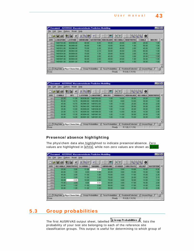
Presence/absence highlighting
The phys/chem data also highlighted to indicate presence/absence. Zero values are highlighted in white, while non-zero values are shown as green.
5.3 Group probabilities
The first AUSRIVAS output sheet, labelled , lists the probability of your test site belonging to each of the reference site classification groups. This output is useful for determining to which group of
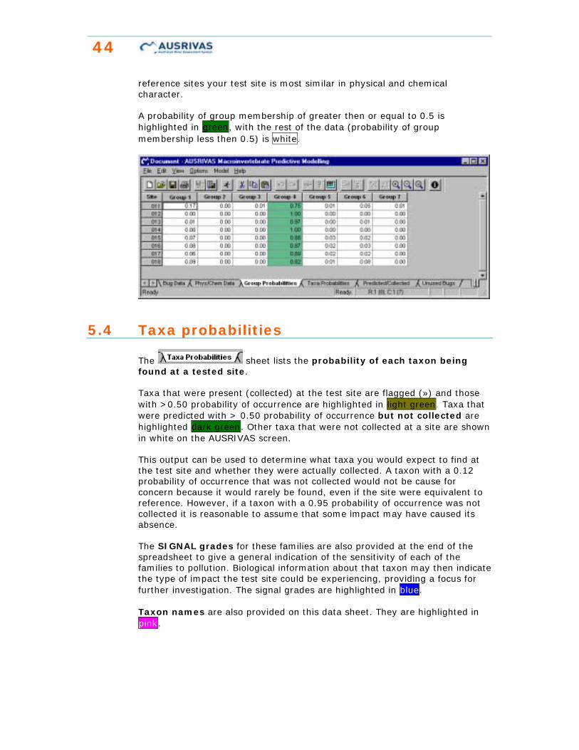
44
reference sites your test site is most similar in physical and chemical character.
A probability of group membership of greater then or equal to 0.5 is highlighted in green, with the rest of the data (probability of group membership less then 0.5) is white.
5.4 Taxa probabilities
The sheet lists the probability of each taxon being found at a tested site.
Taxa that were present (collected) at the test site are flagged (») and those with >0.50 probability of occurrence are highlighted in light green. Taxa that were predicted with > 0.50 probability of occurrence but not collected are highlighted dark green. Other taxa that were not collected at a site are shown in white on the AUSRIVAS screen.
This output can be used to determine what taxa you would expect to find at the test site and whether they were actually collected. A taxon with a 0.12 probability of occurrence that was not collected would not be cause for concern because it would rarely be found, even if the site were equivalent to reference. However, if a taxon with a 0.95 probability of occurrence was not collected it is reasonable to assume that some impact may have caused its absence.
The SIGNAL grades for these families are also provided at the end of the spreadsheet to give a general indication of the sensitivity of each of the families to pollution. Biological information about that taxon may then indicate the type of impact the test site could be experiencing, providing a focus for further investigation. The signal grades are highlighted in blue.
Taxon names are also provided on this data sheet. They are highlighted in pink.

U s e r m a n u a l 45
Hint
The orange highlighting of sites 012 and 014 in this example indicate that these sites are nearly outside the experience of the model. More information on this can be found in Sections 6.4.1 and 6.4.2.
5.5 Predicted/collected
The predicted/collected data sheet provides an assessment of biological condition of a test site. The indices produced here are described in the following sections.
5.5.1 Predicted, expected and observed taxa
The first four columns of the predicted/collected data sheet give information on the predicted, expected and observed numbers of taxa.
NTE50
The Number of inverTebrate families Expected with greater than a 50% probability of occurrence, NTE50, is the sum of the probabilities of all the families predicted with greater than a 50% chance of occurrence
NTP50
NTP50 is a count of the Number of inverTebrate families Predicted with greater than a 50% probability of occurrence
NTC50
The inverTebrate families that were predicted above the threshold probability of 50% and which were also Collected at the test site are counted to form the observed (collected) value, NTC50.
OE50
The Observed to Expected ratio, OE50, is the ratio of the number of invertebrate families observed at a site (NTC50) to the number of families expected (NTE50) at that site. OE50 provides a measure of biological impairment at the test site.

46
The output of these four indices is shown in the screen shot below.
5.5.2 Predicted, expected and observed signal
In addition to calculating the expected number of taxa at a test site, AUSRIVAS also calculates the SIGNAL scores for a site. Calculation of the SIGNAL scores uses SIGNAL grades, an assigned value given to each invertebrate family that indicates their sensitivity to pollution. Columns 5 to 10 in the Predicted/Collected data sheet contain the calculated signal scores, each of which is explained below.
E50Signal
E50Signal is the expected signal score for taxa that have a probability of occurrence of greater than or equal to 50%. It is calculated by weighting the probability of occurrence of each predicted taxa (those taxa that have a probability of occurrence of greater than or equal to 50%) by the taxon's SIGNAL Grade, summing these and then dividing the total by the sum of the (unweighted) probabilities of occurrence.
∑
∑
−
−
×= )50(
1
)50(
150
)(
p
p
N
i
ii
N
i
eSignalGradTaxaPE
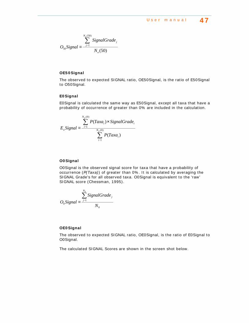
O50Signal
O50Signal is the observed signal score for taxa that have a probability of occurrence of greater than or equal to 50%. It is calculated by averaging the SIGNAL Grade's for all observed taxa with P(Taxa) >= 0.5.
U s e r m a n u a l 47
)50(
)50(
150
o
j
N
j
N
eSignalGradSignalO
o
∑−=
OE50Signal
The observed to expected SIGNAL ratio, OE50Signal, is the ratio of E50Signal to O50Signal.
E0Signal
E0Signal is calculated the same way as E50Signal, except all taxa that have a probability of occurrence of greater than 0% are included in the calculation.
)(
)(
)0(
1
)0(
1
i
N
i
ii
N
io
TaxaP
eSignalGradTaxaPSignalE
p
p
∑
∑
−
−
×=
O0Signal
O0Signal is the observed signal score for taxa that have a probability of occurrence (P(Taxa)) of greater than 0%. It is calculated by averaging the SIGNAL Grade's for all observed taxa. O0Signal is equivalent to the ‘raw’ SIGNAL score (Chessman, 1995).
0
10
0
N
eSignalGradSignalO
j
N
j∑
−=
OE0Signal
The observed to expected SIGNAL ratio, OE0Signal, is the ratio of E0Signal to O0Signal.
The calculated SIGNAL Scores are shown in the screen shot below.
48
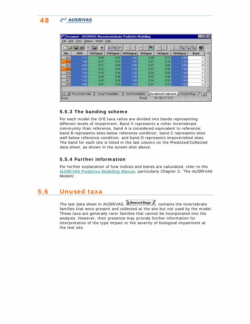
5.5.3 The banding scheme
For each model the O/E taxa ratios are divided into bands representing different levels of impairment. Band X represents a richer invertebrate community than reference, band A is considered equivalent to reference; band B represents sites below reference condition; band C represents sites well below reference condition; and band D represents impoverished sites. The band for each site is listed in the last column on the Predicted/Collected data sheet, as shown in the screen shot above.
5.5.4 Further information
For further explanation of how indices and bands are calculated, refer to the AUSRIVAS Predictive Modelling Manual, particularly Chapter 3, 'The AUSRIVAS Models'.
5.6 Unused taxa
The last data sheet in AUSRIVAS, , contains the invertebrate families that were present and collected at the site but not used by the model. These taxa are generally rarer families that cannot be incorporated into the analysis. However, their presence may provide further information for interpretation of the type impact or the severity of biological impairment at the test site.

U s e r m a n u a l 49
Hint
Always check that the taxon codes listed in the "Unused Bugs" sheet are spelled correctly. If the taxon codes are incorrect, your data will have been unintentionally omitted.
Hint
The data shown in the Unused Bug sheet has been moved here from the input data sheet 'Bug Data', so if you export the 'Bug Data' sheet after running a model, it will not have the bugs listed in the 'Unused Bugs' sheet in it.
5.7 Model information
Along with the output data sheets produced by AUSRIVAS, you can also obtain information about the models. The information available is
! Required predictor variables for each model;
! O/E bands for each model.
Both these sets of information can be obtained from the 'Model' menu. Select 'Required Variables ...' to view lists of predictor variables, or 'Bandwidth ...' to view O/E-taxa bands.
50
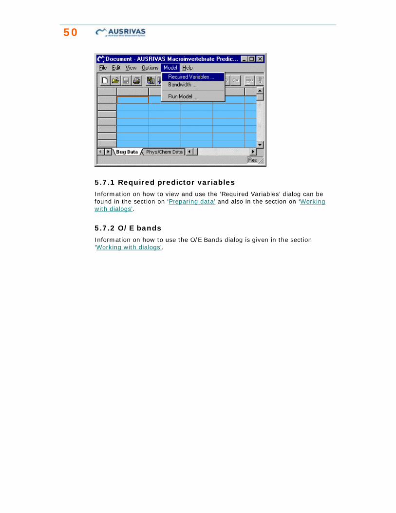
5.7.1 Required predictor variables
Information on how to view and use the ‘Required Variables’ dialog can be found in the section on ‘Preparing data’ and also in the section on ‘Working with dialogs’.
5.7.2 O/E bands
Information on how to use the O/E Bands dialog is given in the section ‘Working with dialogs’.
U s e r m a n u a l 51
Chapter 6: Troubleshooting guide
6.1 Internet access problems
6.1.1 Cannot connect to AUSRIVAS server
Symptoms
When attempting to run AUSRIVAS v3 or below, an error message similar to one of the following is generated:
! Unable to create empty document
! AUSRIVAS error: cannot connect to the AUSRIVAS server
Description of problem
Incorrect Proxy Settings
Your proxy settings may not be correct. When the AUSRIVAS program starts, it attempts to connect to the AUSRIVAS server. If this attempt fails, and you have selected to work in on-line mode, you may get an error similar to the above.
Network down
Part of the network at your site, or at the University of Canberra, where the AUSRIVAS data server is located, may be temporarily down.
Solution
Incorrect Proxy Settings
Find out the details of and configure your proxy server settings as described in Configuring the software for Internet access. Consult your local systems administrator if the problem persists.
Network down
Try the software again later. Consult your local systems administrator if the problem persists.
6.1.2 Proxy authentication required.
Symptoms When attempting to run AUSRIVAS v2.2 or below, an error message similar to one of the following is generated:
HTTP error 407 : Proxy authentication required
Description of problem
AUSRIVAS Version 2.2 and below
AUSRIVAS 2.2 and below does not support proxy authentication. If your proxy server requires authentication (i.e. you have to provide a username and password to access the Internet) then you will need to upgrade to version 3.0 or above.
52
AUSRIVAS Version 3.0 and above
Your proxy authentication settings in AUSRIVAS are possibly not correct.
Solution
AUSRIVAS Version 2.2 and below
Upgrade the AUSRIVAS Macroinvertebrate Predictive Modelling Software to version 3.0 or above, as described in Chapter 3, ‘Obtaining the software’.
AUSRIVAS Version 3.0 and above
Following the procedure outlined in Configuring the software for Internet access make sure that your proxy server settings and your Internet username and password are correct. Consult your local systems administrator if the problem persists.
6.1.3 The system cannot find the file specified.
Symptoms
When attempting to run AUSRIVAS, an error message similar to the following is generated:
The system cannot find the file specified. Internet error number 2.
Description of problem
A user with the following setup experienced this problem:
! Internet: dial-up connection.
! Operating system: MS Windows 2000.
! Internet Explorer: version 5.5.
The problem was traced to Internet Explorer (which was not the users default browser) being set to "work offline".
Solution
Set Internet Explorer to work online.
6.2 DLL errors
6.2.1 MFC42.DLL error
Symptoms
When attempting to run AUSRIVAS v2.2 or above for the first time on a new machine, an error message similar to one of the following is generated:
! OG80AS.DLL is linked to missing export MFC42.DLL:6605
! The ordinal 6883 could not be located in the dynamic link library MFC42.DLL

U s e r m a n u a l 53
Description of problem
Your MS Windows dynamic link library, mfc42.dll, is too old for AUSRIVAS version 2.2 and above. This file needs to be version 6.x or above, while you probably have version 4.x.
To check the version number of your mfc42.dll file, do the following:
1 Locate the file mfc42.dll. This can be done using "Find file" in Windows Explorer. If you find multiple copies of mfc42.dll, look at the one in you Windows directory, i.e. \windows\system, \windows\system32 or \winNT\system32.1
2 View the files’ properties. These can be viewed by right clicking on the file and selecting "Properties" from the drop-down menu.
3. Read the version number. The second tab on the ‘properties’ window contains the version number of the file.
Mfc42.dll contains code, dialogs etc used by Windows, and comes with the MS Windows operating system.
1 In order to locate this file, you may have to change your view under Explorer to show all files. Do this by selecting "Options" under the "View" menu. The window that appears will be different depending on which system you are running, but basically you want to select "show all files" and deselect "hide file extensions of known type" or "hide MS-DOS file extensions for file types that are registered".
Solution
As the file mfc42.dll is part of your MS Windows operating system, you will need to get your systems administrator to update it to version 6 or later.
For those who can’t wait, you can download a copy of mfc42.dll version 6.0.8447.0 and use it at your own risk. So that you can recover if necessary, copy your current mfc42.dll to a "safe place" under a new name (i.e. mfc42_version4.dll) first. Then just copy the version you have downloaded to \Windows\System\mfc42.dll and then re-run AUSRIVAS - it should now work.
6.2.2 Error when selecting the 'Help/About ...' menu or when clicking on the 'Help' button in the 'Internet Settings' dialog.
Symptoms
You get an error message similar to the one below when you select the 'Help/About ...' menu or when clicking on the 'Help' button in the 'Internet Settings' dialog.
54
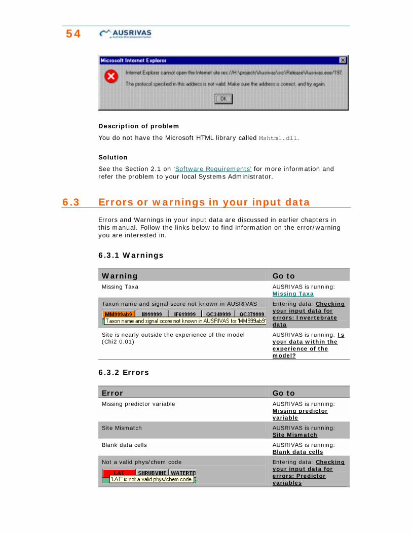
Description of problem
You do not have the Microsoft HTML library called Mshtml.dll.
Solution
See the Section 2.1 on ‘Software Requirements’ for more information and refer the problem to your local Systems Administrator.
6.3 Errors or warnings in your input data
Errors and Warnings in your input data are discussed in earlier chapters in this manual. Follow the links below to find information on the error/warning you are interested in.
6.3.1 Warnings Warning Go to Missing Taxa AUSRIVAS is running:
Missing Taxa
Taxon name and signal score not known in AUSRIVAS Entering data: Checking your input data for errors: Invertebrate data
Site is nearly outside the experience of the model (Chi2 0.01)
AUSRIVAS is running: Is your data within the experience of the model?
6.3.2 Errors Error Go to Missing predictor variable AUSRIVAS is running:
Missing predictor variable
Site Mismatch AUSRIVAS is running: Site Mismatch
Blank data cells AUSRIVAS is running: Blank data cells
Not a valid phys/chem code
Entering data: Checking your input data for errors: Predictor variables
U s e r m a n u a l 55
Site is outside the experience of the model (Chi2 0.001) AUSRIVAS is running: Is your data within the experience of the model?
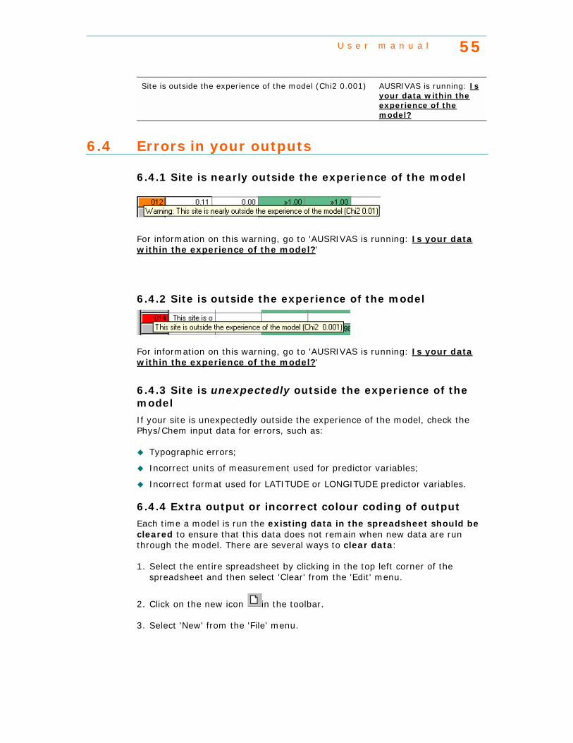
6.4 Errors in your outputs
6.4.1 Site is nearly outside the experience of the model
For information on this warning, go to 'AUSRIVAS is running: Is your data within the experience of the model?'
6.4.2 Site is outside the experience of the model
For information on this warning, go to 'AUSRIVAS is running: Is your data within the experience of the model?'
6.4.3 Site is unexpectedly outside the experience of the model
If your site is unexpectedly outside the experience of the model, check the Phys/Chem input data for errors, such as:
! Typographic errors;
! Incorrect units of measurement used for predictor variables;
! Incorrect format used for LATITUDE or LONGITUDE predictor variables.
6.4.4 Extra output or incorrect colour coding of output
Each time a model is run the existing data in the spreadsheet should be cleared to ensure that this data does not remain when new data are run through the model. There are several ways to clear data:
1. Select the entire spreadsheet by clicking in the top left corner of the spreadsheet and then select 'Clear' from the 'Edit' menu.
2. Click on the new icon in the toolbar.
3. Select 'New' from the 'File' menu.
56
6.5 Running large data sets
6.5.1 Performance scalability
I've analysed the performance scalability of the AUSRIVAS Macroinvertebrate Predictive Modelling software in relation to large data sets, and found the following:
Windows 98/95 memory management doesn't appear to be as efficient as Windows NT. I tested Win98 with 2500 sites and 256Mb memory and the program ran out of memory after processing only 380 sites. I then tested Win NT with 2500 sites and 128Mb memory (plus 180Mb virtual memory), and this succeeded. The AUSRIVAS program was using 4Mb of memory for each 100 sites that it processed. By the end of processing all 2500 sites it was using 181Mb of memory (this includes the operating system and some initial memory used by the AUSRIVAS program as well as the 4Mb per 100 sites). This took over 30 minutes to run on a 550MHz machine.
I then tested Win NT with 4500 sites. I was not able to complete the test because my machine does not have enough memory. However, I was able to see that in this case, the rate of memory usage was 7Mb per 100 sites with an initial overhead of 120Mb. This means that the projected estimate for the amount of memory required to process 4500 sites is at least 436Mb (say 512Mb). I estimate that this would take several hours to run on a 550MHz machine.
I recommend that this be made up of actual physical memory rather than being made up of real and virtual memory (memory temporarily stored to disk) otherwise processing will be slowed greatly.
6.5.2 Summary
In summary (by Operating System):
Windows 95/98
These operating systems can run a maximum of 380 sites, regardless of the machines physical memory and processor speed. (NB some users report a different number of sites for Win 98).
Windows NT
NT can run large data sets. In this case the machines memory (both physical and virtual) restricts how many sites can be run, while the processor speed and proportion of physical to virtual memory determines how long the run will take.
6.5.3 Recommendations
The minimum recommended system to run 4500 sites is:
Operating system: Windows NT
Physical memory: 512Mb
U s e r m a n u a l 57
Depending on processor speed, it could take several hours to run 4500 sites. I’ll update this when I get feedback from users who have run large data sets.
58
Chapter 7: Frequently asked questions
7.1 What is the Chi2 test?
The Chi2 test is used to determine if a test site falls within the experience of the AUSRIVAS model. Any test sites with no appropriate reference group for comparison are identified as being 'outside the experience of the model'
AUSRIVAS determines that a site is outside the experience of the model if its critical value is within the 0.1 percent area (alpha = 0.001) in the tail of the Chi2 distribution.
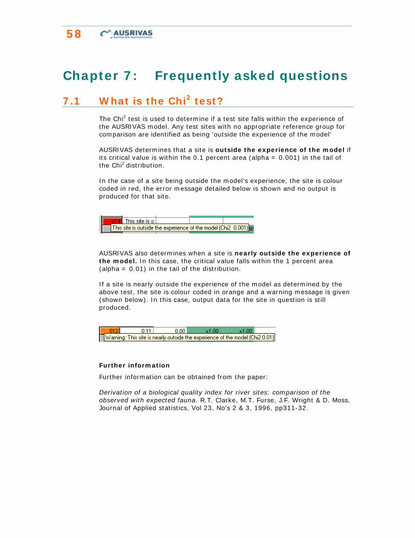
In the case of a site being outside the model’s experience, the site is colour coded in red, the error message detailed below is shown and no output is produced for that site.
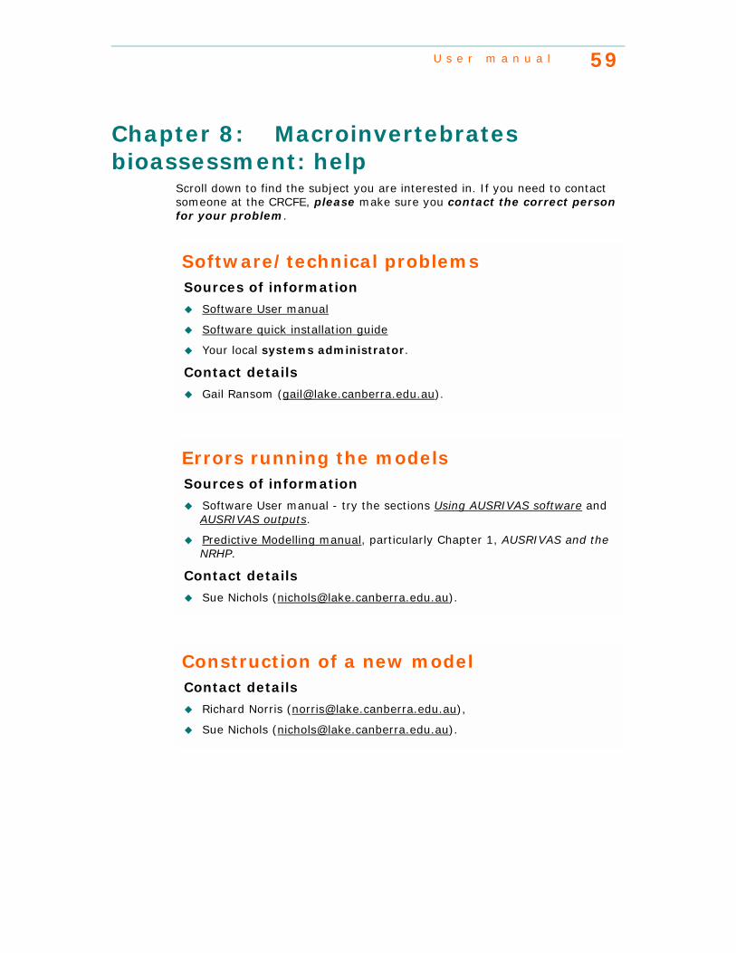
AUSRIVAS also determines when a site is nearly outside the experience of the model. In this case, the critical value falls within the 1 percent area (alpha = 0.01) in the tail of the distribution.
If a site is nearly outside the experience of the model as determined by the above test, the site is colour coded in orange and a warning message is given (shown below). In this case, output data for the site in question is still produced.
Further information
Further information can be obtained from the paper:
Derivation of a biological quality index for river sites: comparison of the observed with expected fauna. R.T. Clarke, M.T. Furse, J.F. Wright & D. Moss. Journal of Applied statistics, Vol 23, No's 2 & 3, 1996, pp311-32.
U s e r m a n u a l 59
Chapter 8: Macroinvertebrates bioassessment: help
Scroll down to find the subject you are interested in. If you need to contact someone at the CRCFE, please make sure you contact the correct person for your problem.
Software/technical problems Sources of information
! Software User manual
! Software quick installation guide
! Your local systems administrator.
Contact details
! Gail Ransom ([email protected]).
Errors running the models Sources of information
! Software User manual - try the sections Using AUSRIVAS software and AUSRIVAS outputs.
! Predictive Modelling manual, particularly Chapter 1, AUSRIVAS and the NRHP.
Contact details
! Sue Nichols ([email protected]).
Construction of a new model Contact details
! Richard Norris ([email protected]),
! Sue Nichols ([email protected]).
60
For Information on coverage of models Sources of information
! Models lists
Contact details
! Contact your State or Territory NRHP Representative.
Manuals On-line or downloadable manuals
! Software user manual
! Predictive modelling manual
Contact details
! Sue Nichols ([email protected]),
! Gail Ransom ([email protected]).
Problems with your password Sources of information
! Obtain a Password
Contact details
! Gail Ransom ([email protected]).