-- --

Preemptive Scheduling Of Uniform Processors With Memory*

Ten-Hwang Lai and Sartaj Sahni

University of Minnesota

Abstract

We consider the problem of preemptively scheduling n jobs on a system of m uniform processors.

Each job has a release time, a due time, and a memory requirement associated with it. Each pro-

cessor has a speed and a memory capacity associated with it. Linear programming formulations

are obtained for the following optimization criteria: (1) minimize the schedule length and (2)

minimize the maximum lateness. We also consider three special cases with the former optimiza-

tion criteria. For each of these cases, low order polynomial time algorithms are obtained.

Keywords and Phrases

preemptive scheduling, uniform processors, memories, release time, due time, Cmax, Lmax, linear

programming, complexity.

* This research was supported in part by the Office of Naval Research under contract N00014-

80-C-0650.

1

-- --

2

1. Introduction

Let J = { Ji | 1 ≤ i ≤ n } be a set of independent jobs. Associated with each job, Ji, is a 4-tuple

(ti, mi , ri , di) where ti is the job’s processing time (ti > 0), mi is its memory requirement, ri is its

release time, and di is its due time. Let P = { Pi | 1 ≤ i ≤ m } be a set of m processors. With each

processor, Pi, there is a 2-tuple (si, µi) associated. si is the speed of Pi and µi is its memory capa-

city. Job Ji (or simply job i) can be run on processor Pj (or simply processor j) iff mi ≤ µj. Furth-

ermore, it takes Pj ti/sj time to completely run job Ji. P is said to be a uniform processor system

with memories. If s1 = s2 = . . . = sm, then P is a system of identical processors with memories.

If s1 = s2 = . . . = sm and µ1 = µ2 = . . . = µm, P is simply a system of identical processors.

Finally, if µ1 = µ2 = . . . = µm, P is called a system of uniform processors.

A feasible preemptive schedule S for job set J on the processor system P is an assignment

of jobs to time slots on processors such that:

(a) No job is processed by more than one processor at any given time.

(b) No processor executes more than one job at any given time.

(c) The total processing assigned for each job equals its processing requirement.

(d) No job is processed by a processor with memory capacity less than the job’s memory

requirement.

(e) No job is processed before its release time.

S is a nonpreemptive schedule iff, in S, each job is processed continuously, on the same

processor, from its start to finish.

The finish time, fi, of job i in schedule S, is the time at which its processing is completed.

The length (or finish time), Cmax(S), of schedule S is the least time by which all jobs have been

processed. I.e.,

Cmax(S) = i

max{fi}

The Cmax problem is that of determining a schedule S for which Cmax(S) is minimum

amongst all feasible schedules. Let S be a feasible schedule. Li = fi − di is the lateness of job i, 1

≤ i ≤ n. Lmax(S) = maxi{Li} is the maximum lateness of any job in S. The Lmax problem is that of

determining a schedule with minimum Lmax.

When S is restricted to be a non-preemptive schedule, the Lmax problem is known to be NP-

hard even when m = 1 [3]. Under this same restriction, the Cmax problem is NP-hard even when

m = 2, s1 = s2, µ1 = µ2, and r1 = r2 = ... = rn [3]. In the remainder of this paper, we shall therefore

be concerned only with schedules in which preemptions are permitted.

Suppose that P is a system of identical processors (i.e., s1 = s2 = ... = sm and µ1 = µ2 = ... =

µm). When all jobs have the same release time (r1 = r2 = ... = rn) a schedule that minimizes Cmax

-- --

3

can be obtained in O(n) time using McNaugton’s algorithm [12]. When the release times are not

necessarily the same, a schedule that minimizes Cmax can be obtained in O(nm) time using the

algorithm of Gonzalez and Johnson [5].

If P is a uniform processor system (µ1 = µ2 = ... = µm) and all jobs have the same release

time, a schedule minimizing Cmax may be obtained in O(n + mlogm) time using the algorithm of

Gonzalez and Sahni [7]. When the release times are not necessarily the same, the algorithm of

Sahni and Cho [14] may be used. This algorithm has a complexity of O(m2n + mnlogn).

Scheduling on processor systems with memories has been studied by Kafura and Shen [8]

as well as by Lai and Sahni [11]. Both these papers deal exclusively with a system of identical

processors with memory. Kafura and Shen [8] develop an O(nlogm), n ≥ m, algorithm for the

Cmax problem when all release times are the same. Lai and Sahni [11] consider the Lmax problem

when all release times are the same. Their algorithm is of complexity O(k 2n + nlogn) where k is

the number of distinct due dates and n ≥ m.

In this paper, we consider scheduling systems of uniform processors with memories. In

Section 2, we obtain linear programming formulations for the Cmax and Lmax problems. Three

special cases of Cmax problem are considered in Section 3. Each of these cases assumes that all

jobs are released at the same time (i.e., r1 = r2 = ... = rn). In addition, the three cases, respec-

tively, assume:

(1) m = 2

(2) m = 3

(3) The m processors can be partitioned into two classes A and B such that all processors in A

have the same speed while all those in B have the same memory size. In addition, all pro-

cessors in A have a larger memory size than those in B. So, for some ordering of the pro-

cessors, it is the case that µ1 ≥ µ2 ≥ ... ≥ µk > µk +1 = ... = µm and s1 = s2 = ... = sk.

For each of the above three cases, we develop low order polynomial time algorithms.

2. Linear Programming Formulations

Let J be a set of n jobs and let P be a set of m processors. Without loss of generality, we assume

that µ1 ≥ µ2 ≥ ... ≥ µm. Furthermore, let S be any schedule for J on P. The following notation will

prove useful in obtaining the linear programming formulations.

(a) h(i) is the largest index such that job i can be processed on Ph (i). I.e., h(i) = max { j | mi ≤ µj

}.

(b) q1, q2, ..., qu are the distinct release times in the multiset { r1, r2, ..., rn } and q1 < q2 < ... <

qu . Let qu +1 denote the length of S (i.e., qu +1 = Cmax(S)). Clearly, qu < qu +1.

(c) r(i) is such that ri = qr (i), 1 ≤ i ≤ n.

-- --

4

(d) xijk denotes the amount of time for which job i is assigned to procesor j (or Pj) in the inter-

val [qk, qk +1], 1 ≤ i ≤ n, 1 ≤ j ≤ m, 1 ≤ k ≤ u.

2.1 The Cmax Problem

It is clear that for every feasible schedule S the xijks satisfy the following constraints ( (2.1) - (2.4)

):

j =1Σm

xijk ≤ qk +1 − qk, 1 ≤ i ≤ n, 1 ≤ k ≤ u (2.1)

I.e., no job is scheduled in any interval for an amount of time greater than the interval length.

i =1Σn

xijk ≤ qk +1 − qk, 1 ≤ j ≤ m, 1 ≤ k ≤ u (2.2)

I.e., no processor is scheduled in any interval for an amount of time greater than the interval

length.

j =h (i)+1Σm

xijk = 0, 1 ≤ i ≤ n, 1 ≤ k ≤ u (2.3a)

I.e., no job is assigned to a processor with insufficient memory.

k =1Σ

r (i)−1

xijk = 0, 1 ≤ i ≤ n, 1 ≤ j ≤ m (2.3b)

I.e., no job is processed before its release time.

j =1Σm

k =1Σu

xijksj = ti, 1 ≤ i ≤ n (2.3c)

I.e., each job is completed.

And

xijk ≥ 0, 1 ≤ i ≤ n, 1 ≤ j ≤ m, 1 ≤ k ≤ u (2.4)

I.e., all assignments are for a nonnegative amount of time.

One readily sees that if the xijks satisfy the above constraints, then they also satisfy the

requirements of the Gonzales-Sahni [6] theorem for open shop scheduling. Hence, their algo-

rithm can be used to obtain a feasible schedule of length qu +1 in which job i is scheduled on pro-

cessor j in interval [qk, qk +1] for exactly xijk time. So, a schedule that minimizes Cmax can be

obtined by first solving the linear programming program:

minimize qu +1

-- --

5

subject to constraints (2.1), (2.2), (2.3a), (2.3b),

(2.3c) and (2.4).

Once the xijks and qu +1 have been obtained, the schedule can be constructed, interval by interval,

using the algorithm for open shop scheduling [6]. It is not too difficult to see that the n(u+m+1)

equalities corresponding to (2.3a), (2.3b), and (2.3c) can be replaced by the n equalities:

j =1Σh (i)

k =r (i)Σu

xijksj = ti, 1 ≤ i ≤ n (2.3)

in the above linear programming formulation. In addition, the variables

xijk, h (i)+1 ≤ j ≤ m, 1 ≤ k ≤ r(i)-1, 1 ≤ i ≤ n

may be set to zero. This transformation reduces the total number of variables and inequalities

and so results in a simpler linear program.

The most practical way to solve the formulated linear program is via the simplex method.

This is known to have a good expected performance (see Dantzig [1]). The simplex method does

however have an exponential worst case performance ([4] and [10]). It should be pointed out that

Khachian [9] has obtained a polynomial time algorithm to solve linear inequalities. His algo-

rithm has a worst case complexity that is O(Ln2(mn+n2)), where m is the number of inequalities;

n the number of variables; and L the number of bits needed to represent all the coefficients. Gacs

and Lovasz [2] describe how linear programming problems can be reduced to solving systems of

inequalities.

From the results of Khachian [9], Gacs and Lovasz [2], Gonzalez and Sahni [6], and our

linear programming formulation, it follows that the Cmax problem can be solved in polynomial

time.

2.2 The Lmax Problem

Let S* be a schedule that minimizes Lmax. Let y* = Lmax(S*). It is not too difficult to see that y*

is the smallest y for which the job set characterized by (ti, mi, ri, di + y), 1 ≤ i ≤ n, has a schedule

S with Lmax(S) ≤ 0.

Let y be arbitrary. We may determine whether or not there is a schedule for (ti, mi, ri, di +

y), 1 ≤ i ≤ n that has an Lmax ≤ 0 as follows. First sort the distinct release and due times in the

multiset

{ ri | 1 ≤ i ≤ n } U { di + y | 1 ≤ i ≤ n } (2.5)

to get the ordered set (q1, q2, ..., qu), q1 < q2 < ... < qu. Let r(i) and d(i) be such that ri = qr (i) and di

-- --

6

+ y = qd (i), 1 ≤ i ≤ n. From the development of Section 2.1, it follows that there is a schedule with

Lmax ≤ 0 iff the following linear system has a feasible solution (xijk denotes the amount of time for

which job i is scheduled on Pj in the interval [qk, qk +1]).

j =1Σm

xijk ≤ qk +1 − qk, 1 ≤ i ≤ n, 1 ≤ k < u (2.6)

i =1Σn

xijk ≤ qk +1 − qk, 1 ≤ j ≤ m, 1 ≤ k < u (2.7)

j =1Σh (i)

k =r (i)Σ

d (i)−1

xijksj = ti, 1 ≤ i ≤ n (2.8)

xijk ≥ 0, 1 ≤ i ≤ n, 1 ≤ j ≤ m, 1 ≤ k < u (2.9)

To determine y* (the least y for which a schedule with Lmax ≤ 0 exists), construct the set ∆

= { δ | di + δ = rj for some i and j }. Note that | ∆ | ≤ n2 and ∆ may contain both positive and

negative elements. Let δ1, δ2, ..., δp be the elements of ∆. We may assume that δ1 < δ2 < ... < δp .

Since δ1 = mini{ri} - maxi{di}, di + δ1 ≤ ri for every i. Hence, there is no schedule with Lmax ≤ 0

when the job characteristics are (ti, mi , ri , di + δ1), 1 ≤ i ≤ n.

The next step in determining y* is to find the largest j such that there is no schedule with

Lmax ≤ 0 for (ti, mi, ri, di + δ j), 1 ≤ i ≤ n. This can be done by carrying out a binary search over the

δis and using the formulation (2.6) - (2.9) to determine the existence of a schedule with Lmax ≤ 0.

Let this largest j be w. If w = p, then we may define δp +1 = ∞ for convenience. It is now clear

that δw < y* ≤ δw +1. Let (q1, q2, ..., qu) be the ordered set of distinct release and due times

obtained when y is set equal to δw in (2.5). Let δ be arbitrary. If qi corresponds to a dj + δw but

no rk, then replace it by d j + δ. If qi corresponds to both an rk and a dj + δw then insert d j + δ into

the sequence of qis immediately after qi. Let the new sequence be (q´1, q´2, ..., q´u´), u’ ≥ u. Note

that for δw < δ < δw +1 , q´1 < q´2 < ... < q´u´ . Consequently, for δ in this range, the r and d functions

defined by ri = q´r (i) and di + δ = q´d (i) do not change with δ. This allows us to formulate the fol-

lowing linear program:

minimize δ

subject toj =1Σm

xijk ≤ q´k +1 - q´k, 1 ≤ i ≤ n, 1 ≤ k < u’

i =1Σn

xijk ≤ q´k +1 - q´k, 1 ≤ j ≤ m, 1 ≤ k < u’

-- --

7

j =1Σh (i)

k =r (i)Σ

d (i)−1

xijksj = ti, 1 ≤ i ≤ n

δw < δ < δw +1

xijk ≥ 0, 1 ≤ i ≤ n, 1 ≤ j ≤ m, 1 ≤ k < u’

From our earlier discussions, it follows that if the above linear program has no feasible

solution, then y* = δw +1; if it does then y* is the min δ obtained above. Once y* has been

obtained, a schedule with Lmax = y* is easily constructed.

In conclusion, we note that the Lmax algorithm described can be implemented in polynomial

time.

3. Special cases

In this section, we assume that all jobs are released at time 0. Since only the Cmax problem is

considered, we ignore the due times that may be specified. Under the preceding restriction on the

release times, the Cmax problem is studied for the following cases:

(1) m = 2

(2) m = 3

(3) The m processors can be partitioned into two classes A and B such that all processors in A

have the same speed while all those in B have the same memory size. In addition, all pro-

cessors in A have a larger memory than those in B.

In order to establish the correctness of our algorithms, we shall make use of an important

result from Sahni and Cho [13]. Let Pi, 1 ≤ i ≤ m be m processors with the same memory size.

Let si(t), 1 ≤ i ≤ m be m nondecreasing functions; si(t) gives the speed at which Pi may operate at

time t. {P1, P2, ..., Pm} is a generalized processor system (GPS) iff si(t) ≥ si +1(t), 1 ≤ i < m for all

t.

Theorem 1 [Sahni and Cho]: Let ti, 1 ≤ i ≤ n be n job times such that t1 ≥ t2 ≥ ... ≥ tn. Let {P1, P2 ,

..., Pm} be a GPS and let Tk =i =1Σk

ti, 1 ≤ k < m and Tm =i =1Σn

ti ( if n < m, then set Tn +1 = Tn +2 = ... =

Tm). The given n jobs can be scheduled on the given GPS to finish by time d iff:

Ti ≤j =1Σ

i

0∫d

sj(t)dt, 1 ≤ i ≤ m. []

One can prove that the preceding theorem is true even if the restriction that si(t) is a nonde-

creasing function of t is removed. (Actually, Sahni and Cho’s proof in [13] does not use the pro-

perty that si(t) is nondecreasing.) Suppose that H1, H2, and H3 form a relaxed GPS, A, (i.e., one

-- --

8

that satisfies all the requirements of a GPS except that si(t) may not be a nondecreasing function

of t). Let Li = 0∫d

si(t)dt, 1 ≤ i ≤ 3. Let L´i, 1 ≤ i ≤ 3 be the corresponding values for some other

relaxed GPS, B. If L1 ≥ L´1 , L1 + L2 ≥ L´1 + L´2, and L1 + L2 + L3 ≥ L´1 + L´2 + L´3, then it follows

that every job set that can be scheduled to complete by d on B can also be scheduled to complete

by d on A. This observation will be implicitly used in Section 3.2.

3.1 m = 2

Without loss of generality, assume that µ1 ≥ µ2 and mi ≤ µ1, 1 ≤ i ≤ n. Let n1 be such that mi > µ2 ,

1 ≤ i ≤ n1, and either n1 = n or mi ≤ µ2, n1 < i ≤ n (it may require a job reordering to guarantee

such a n1). So, jobs 1, 2, ..., n1 must be scheduled on P1 while jobs n1+1, n1+2, ..., n may be

scheduled on either P1 or P2. Further, assume that tn 1+1 ≥ ti, n1 + 2 ≤ i ≤ n. We first observe that

if there is a schedule S for the n jobs such that Cmax(S) = d, then there is a schedule with the same

finish time d in which jobs 1, 2, ..., n1 are scheduled on P1 from time 0 to time τ = (i =1Σn 1

ti)/s1 (see

Figure 1).

Figure 1

To see this, note that the schedule S can be divided into intervals with the property that in each

interval the jobs scheduled on P1 are either all from {1, 2, ..., n1} or all from {n1+1, n1+2, ..., n}.

Once this division into intervals has been done, we can easily construct, by interchanging inter-

vals, a new schedule, S’, in which all intervals containing jobs from {1, 2, ..., n1} are at the left.

S’ has a finish time d.

Hence, the Cmax problem when m = 2 reduces to finding a minimum finish time schedule for

-- --

9

jobs {n1+1, ..., n} on a two processor system {Q1 , Q2} in which Q1 operates at speed 0 from time

0 to τ and at speed s1 after τ; and Q2 operates at speed s2 from time 0. Furthermore, we may

assume that Q1 and Q2 have the same memory size. If s2 ≥ s1, then {Q2, Q1} forms a GPS. If s2

< s1 , then a GPS {R1, R2} equivalent to {Q1, Q2} may be formed by assigning to R1 a speed of s2

from 0 to τ and s1 from τ on; R2 has a speed of 0 from 0 to τ and s2 from τ on (see Figure 2).

Figure 2 Forming the GPS

From Theorem 1, we see that the jobs n1+1, n1+2, ..., n can be scheduled to complete by d

on the resulting GPS iff

tn 1+1 ≤ s2τ + max{s1, s2}(d - τ)

and

i =n 1+1Σn

ti ≤ s2d + s1(d - τ)

Rearranging terms and combining, we see that d must satisfy the inequality:

d ≥ max{max{s1 , s2}

tn 1+1 − s2τ___________ + τ, s1 + s2

T2 + s1τ________}

where T2 =i =n 1+1Σn

ti. Let T1 =i =1Σn 1

ti. Substituting τ = T1/s1 and adding the requirement that d ≥ τ,

we obtain:

d ≥ max{s1

T1___, max{s1 ,s2}

tn 1+1−s2T1/s1____________ + s1

T1___, s1+s2

T1+T2_______} (3.1)

-- --

10

We immediately see that the minimum Cmax is given by the right hand side of (3.1).

To summarize, a minimum Cmax schedule for 2 processors with memories can be obtained

by following the steps given below:

Step 1: Determine n1 as given above (reorder the jobs if necessary).

Step 2: Schedule jobs 1, 2, ..., n1 on P1 from 0 to τ = i =1Σn 1

ti/s1

Step 3: Compute the right hand side of (3.1). Let this value be δ.

Step 4: Construct the GPS as in Figure 2. Schedule jobs n1+1, ..., n on this GPS from 0 to δ

using the algorithm of [13].

Step 5: Map the schedule obtained in step 4 back onto P1 and P2 . This is trivial because of the

obvious correspondence between the GPS and segments of P1 and P2.

Each of the steps above takes O(n) time and the overall complexity of the two processor

algorithm is O(n). In an actual implementation, of course, steps 4 and 5 would be combined and

the schedule constructed directly for P1 and P2.

3.2 m = 3

Assume that µ1 ≥ µ2 ≥ µ3 and that the jobs are ordered such that m1 ≥ m2 ≥ ... ≥ mn (without loss

of generality, we may assume that mi ε {µ1 , µ2 , µ3}, 1 ≤ i ≤ n and so it takes only O(n) time to

order the jobs). Let n1 and n2 be such that jobs 1, 2, ..., n1 are the only jobs that cannot be pro-

cessed on P2 or P3 because of memory requirements and jobs 1, 2, ..., n2 are the only jobs that

cannot be processed on P3 because of memory requirements. Clearly, n1 ≤ n2. For convenience,

we now define tn +1 = tn +2 = 0. Let T1 =i =1Σn 1

ti and T2 =n 1+1Σn 2

ti. Further, assume that tn 1+1 ≥ ti, n1+2 ≤

i ≤ n2 and tn 2+1 ≥ tn 2+2 ≥ ti, n2+3 ≤ i ≤ n.

A finish time d is said to be feasible iff there exists a schedule S for the given n jobs such

that Cmax(S) ≤ d. We shall proceed to obtain a set of necessary and sufficient conditions for d to

be feasible. Once this has been done, we shall see how to find a minimum d satisfying these con-

ditions and to then construct a schedule with minimum finish time.

First, we see that d must satisfy the inequalities of (3.2) below:

i =1Σk

Ti / i =1Σk

si ≤ d, k = 1, 2, 3 (3.2)

For the same reasons as in Section 3.1, we may limit our discussion to schedules in which jobs 1,

2, ..., n1 are scheduled from 0 to d1, d1 = T1 /s1 on P1 (Figure 3(a)). Hence, the scheduling of

n1+1, ..., n2 must be done on the GPS of Figure 3(b). In this figure, σ1 = max { s1, s2 } and σ2 =

min { s1, s2 }.

-- --

11

Figure 3

Let Pfast and Pslow , respectively, denote the processor with speed σ1 and σ2 (if σ1 = σ2, then

fast = 1 and slow = 2). Let C1 = s2d1, and C2 = σ1(d − d1). Hence, C1 is P2´s contribution to G1

from 0 to d1 while C2 is Pfast´s contribution to G1 from d1 to d. Thus the total available process-

ing capability on G1 is C1 + C2. Let C3 = σ2(d2 − d1) be the available processing on G2.

We shall consider three cases for T2: (a) T2 ≤ C3; (b) C3 < T2 ≤ C1 + C3; and (c) C1 + C3 <

T2. When T2 ≤ C3, a possible assignment for jobs n1+1, ..., n2 is to schedule them on G2 from d1

to d2 , d2 = d1 + T2/σ2 (Figure 4(a)). If this is done, the GPS that remains for the remaining jobs is

as in Figure 4(b) where σ3 = max{ s2, s3 }; σ4 = max{ σ1, s3 } = max{ s1, s2 , s3 }; σ5 = min{ s2, s3

}; σ6 = min{ σ1, s3 }; σ7 = max{ σ2, σ6}; and σ8 = min{ σ2, σ6 } = min{ s1 , s2 , s3 }. Let r1(t) and

r2(t), respectively, denote the speed of H1 and H2 at time t, 0 ≤ t ≤ d. We immediately see that

there is no sceduling of jobs n1+1, ..., n2 that yields a larger value for0∫d

r1(t)dt or0∫d

r1(t)dt +

0∫d

r2(t)dt. Hence, from Theorem 1, it follows that (3.2) together with the following ((3.3) and

(3.4)) form a set of necessary and sufficient conditions for d when T2 ≤ C3:

tn 2+1 ≤ σ3d1 + σ4(d − d1)

= d1max{s2 ,s3} + (d−d1)max{s1 ,s2 ,s3} (3.3)

tn 2+1 + tn 2+2 ≤ (σ3+σ5)d1 + (σ4+σ6)(d2−d1) + (σ4+σ7)(d−d2)

= d1(s2+s3) + (d2−d1)(s3+σ1)

-- --

12

+ (d−d2)(s1+s2+s3−min{s1 ,s2 ,s3}) (3.4)

Figure 4

Next, consider the case C3 < T2 ≤ C1 + C3 . If we schedule the jobs n1+1, ..., n2 on G2 from

d1 to d and on G1 from 0 to (T2 - C3)/s2 ( Figure 5(a) ), then we will be left with the GPS of Fig-

ure 5(b). The processing capability, K, of H1 is seen to be :

K = s3(T2 − C3)/s2 + (d1 − (T2 − C3)/s2)max{s2 , s3}

+ (d − d1)max{s1 , s2 , s3}

We also see that no matter how jobs n1+1, ..., n2 are scheduled on G1 and G2 , we cannot

create a generalized processor from the remaining idle times on G1, G2, and P3 such that its

procesing capability from 0 to d exceeds K. The total processing capability remaining on G1, G2 ,

and G3 will of course be the same no matter how jobs n1+1, ..., n2 are scheduled. From these

observations and Theorem 1, we see that if (3.2) is satisfied and C3 < T2 ≤ C1 + C3 then it is both

necessary and sufficient that tn 2+1 ≤ K in order for d to be feasible.

Now, let us consider the final case, T2 > C1 + C3. Let w = d1 + (T2 − C1 − C3)/σ1 . From

(3.2), it follows that T2 ≤ C1 + C2 + C3. This together with T2 > C1 + C3 implies that d1 < w ≤ d.

We shall consider the two subcases: (3a) tn 1+1 ≤ s2d1 + (w - d1)σ1 + (d - w)σ2 and (3b) tn 1+1 > s2d1

+ (w - d1)σ1 + (d - w)σ2. In subcase (3a), we see from Theorem 1 that jobs n1+1, ..., n2 can be

scheduled on G1 and G2 as shown in Figure 6(a). To see this, note that the scheduled portions are

equivalent to the GPS of Figure 6(b) and by Theorem 1, jobs n1+1, ..., n2 can be scheduled on this

-- --

13

Figure 5

GPS.

Figure 6

Once jobs n1+1, ..., n2 have been scheduled on G1 and G2 in this manner, the remaining idle

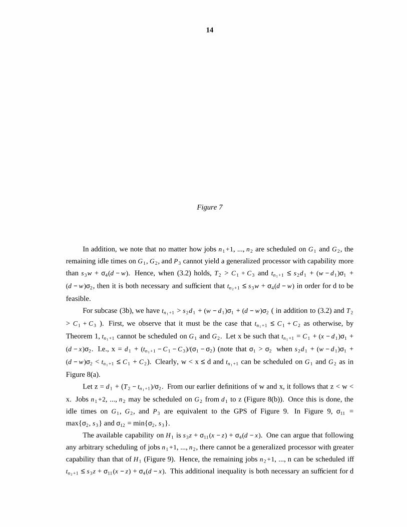
times on G1, G2, and P3 yield the GPS of Figure 7. From Theorem 1, it follows that jobs n2+1, ...,

n can be scheduled on the GPS of Figure 7 iff tn 2+1 ≤ s3w + σ4(d − w).

-- --

14

Figure 7

In addition, we note that no matter how jobs n1+1, ..., n2 are scheduled on G1 and G2, the

remaining idle times on G1, G2, and P3 cannot yield a generalized processor with capability more

than s3w + σ4(d − w). Hence, when (3.2) holds, T2 > C1 + C3 and tn 1+1 ≤ s2d1 + (w − d1)σ1 +

(d − w)σ2 , then it is both necessary and sufficient that tn 2+1 ≤ s3w + σ4(d − w) in order for d to be

feasible.

For subcase (3b), we have tn 1+1 > s2d1 + (w − d1)σ1 + (d − w)σ2 ( in addition to (3.2) and T2

> C1 + C3 ). First, we observe that it must be the case that tn 1+1 ≤ C1 + C2 as otherwise, by

Theorem 1, tn 1+1 cannot be scheduled on G1 and G2. Let x be such that tn 1+1 = C1 + (x − d1)σ1 +

(d − x)σ2. I.e., x = d1 + (tn 1+1 − C1 − C3)/(σ1 − σ2) (note that σ1 > σ2 when s2d1 + (w − d1)σ1 +

(d − w)σ2 < tn 1+1 ≤ C1 + C2). Clearly, w < x ≤ d and tn 1+1 can be scheduled on G1 and G2 as in

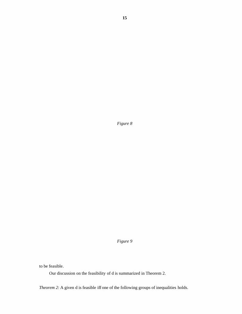
Figure 8(a).

Let z = d1 + (T2 − tn 1+1)/σ2 . From our earlier definitions of w and x, it follows that z < w <

x. Jobs n1+2, ..., n2 may be scheduled on G2 from d1 to z (Figure 8(b)). Once this is done, the

idle times on G1, G2, and P3 are equivalent to the GPS of Figure 9. In Figure 9, σ11 =

max{σ2 , s3} and σ12 = min{σ2 , s3}.

The available capability on H1 is s3z + σ11(x − z) + σ4(d − x). One can argue that following

any arbitrary scheduling of jobs n1+1, ..., n2 , there cannot be a generalized processor with greater

capability than that of H1 (Figure 9). Hence, the remaining jobs n2+1, ..., n can be scheduled iff

tn 2+1 ≤ s3z + σ11 (x − z) + σ4(d − x). This additional inequality is both necessary an sufficient for d

-- --

15

Figure 8

Figure 9

to be feasible.

Our discussion on the feasibility of d is summarized in Theorem 2.

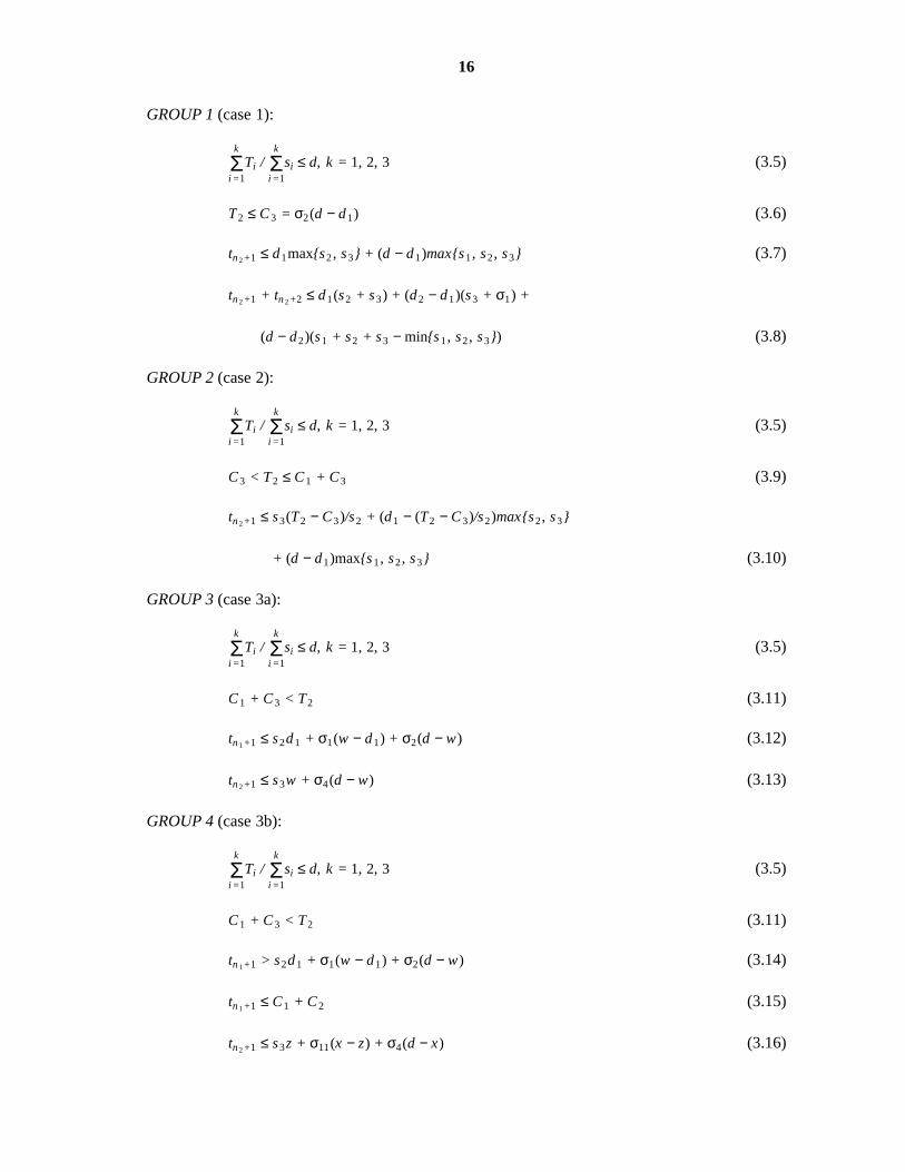
Theorem 2: A given d is feasible iff one of the following groups of inequalities holds.

-- --

16

GROUP 1 (case 1):

i =1Σk

Ti / i =1Σk

si ≤ d, k = 1, 2, 3 (3.5)

T2 ≤ C3 = σ2(d − d1) (3.6)

tn 2+1 ≤ d1max{s2 , s3} + (d − d1)max{s1 , s2 , s3} (3.7)

tn 2+1 + tn 2+2 ≤ d1(s2 + s3) + (d2 − d1)(s3 + σ1) +

(d − d2)(s1 + s2 + s3 − min{s1 , s2 , s3}) (3.8)

GROUP 2 (case 2):

i =1Σk

Ti / i =1Σk

si ≤ d, k = 1, 2, 3 (3.5)

C3 < T2 ≤ C1 + C3 (3.9)

tn 2+1 ≤ s3(T2 − C3)/s2 + (d1 − (T2 − C3)/s2)max{s2 , s3}

+ (d − d1)max{s1 , s2 , s3} (3.10)

GROUP 3 (case 3a):

i =1Σk

Ti / i =1Σk

si ≤ d, k = 1, 2, 3 (3.5)

C1 + C3 < T2 (3.11)

tn 1+1 ≤ s2d1 + σ1(w − d1) + σ2(d − w) (3.12)

tn 2+1 ≤ s3w + σ4(d − w) (3.13)

GROUP 4 (case 3b):

i =1Σk

Ti / i =1Σk

si ≤ d, k = 1, 2, 3 (3.5)

C1 + C3 < T2 (3.11)

tn 1+1 > s2d1 + σ1(w − d1) + σ2(d − w) (3.14)

tn 1+1 ≤ C1 + C2 (3.15)

tn 2+1 ≤ s3z + σ11(x − z) + σ4(d − x) (3.16)

-- --

17

(Note that (3.6), (3.9), and (3.11) are mutually exclusive, also (3.12) and (3.14) are mutually

exclusive. So, for any d, at most one group of inequalities may hold.) []

Each inequality above (3.5 - 3.16) may be rearranged so as to be of the form

d ≥ f( ), d > f( ), d ≤ f( ), or d < f( )

where f is a function of the remaining variables. For each group, one can determine in O(n) time,

the minimum d (if any) that satisfies all inequalities in that group. If no d does, the minimum

may be set to ∞. The minimum of the ds so obtained for the four groups above yields the

minimum Cmax.

Once the Cmax has been determined the corresponding schedule may be constructed in O(n)

time as discussed.

3.3 Two Class of Processors

Let A and B be two classes of processors such that all processors in A have the same speed, sA,

while all in B have the same memory size, µB. Further, assume that the memory size of every

processor in A is greater than that of the processors in B. The n jobs to be scheduled may be par-

tioned into two disjoint sets R and T such that the memory requirement of every job in R exceeds

µB while the memory requirement of every job in T is less than or equal to µB.

It is clear that jobs in R can be scheduled only on processors in A. The set of processors in

A forms a system of identical processors with memory. Kafura and Shen [8] have developed

necessary and sufficient conditions for d to be feasible for a system of identical processors with

memory. Let |A| = a and |R| = r. Assume that µ1 ≥ µ2 ≥ ... ≥ µa and that m1 ≥ m2 ≥ ... ≥ mr. Let Fi

denote the subset of R consisting only of those jobs with memory requirement more than µi +1, 1 ≤

i < a. Let Fa = R. We assume that m1 ≤ µ1. Let Xi be the sum of the processing times of all jobs

in Fi, 1 ≤ i ≤ a. Kafura and Shen [8] have shown that the job set R can be scheduled on the pro-

cessor set A to complete by time d iff d satisfies the inequality:

d ≥ f * = max{ 1≤i≤rmax{ti/sA},

1≤i≤amax{Xi/(sAi)} } (3.17)

Furthermore, when d satisfies the above inequality the desired schedule may be obtained by

scheduling the jobs in the order 1, 2, ..., r using McNaughton’s strategy [12] on the processors in

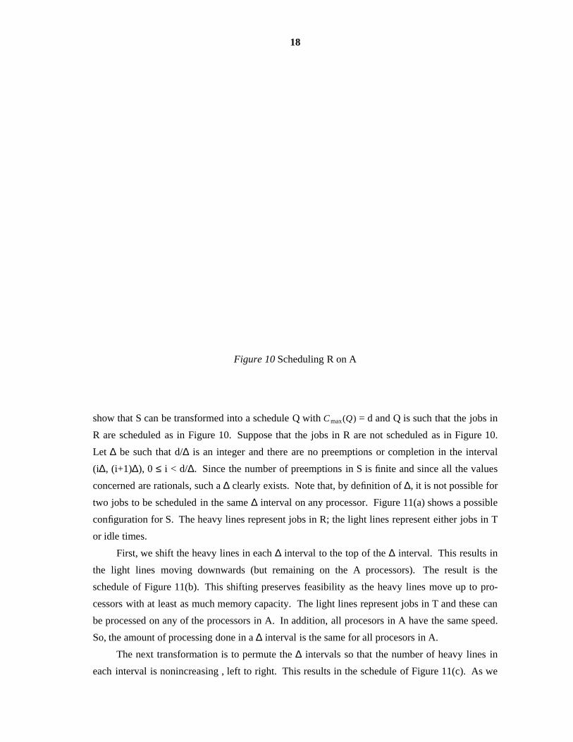
the order 1, 2, ..., a. The resulting schedule fully utilizes processors 1, 2, ..., b where b =

fP(afi=1Σr

ti/(sAd). In addition, if b < a then processor b+1 is utilized from 0 to c = rem(i=1Σr

ti, sAd) / sA

where rem(x, y) is the remainder of x divided by y. Hence the schedule is as in Figure 10.

Let S be any schedule for the jobs in R ∪ T. Let Cmax(S) = d. Clearly, d ≥ f*. We shall

-- --

18

Figure 10 Scheduling R on A

show that S can be transformed into a schedule Q with Cmax(Q) = d and Q is such that the jobs in

R are scheduled as in Figure 10. Suppose that the jobs in R are not scheduled as in Figure 10.

Let ∆ be such that d/∆ is an integer and there are no preemptions or completion in the interval

(i∆, (i+1)∆), 0 ≤ i < d/∆. Since the number of preemptions in S is finite and since all the values

concerned are rationals, such a ∆ clearly exists. Note that, by definition of ∆, it is not possible for

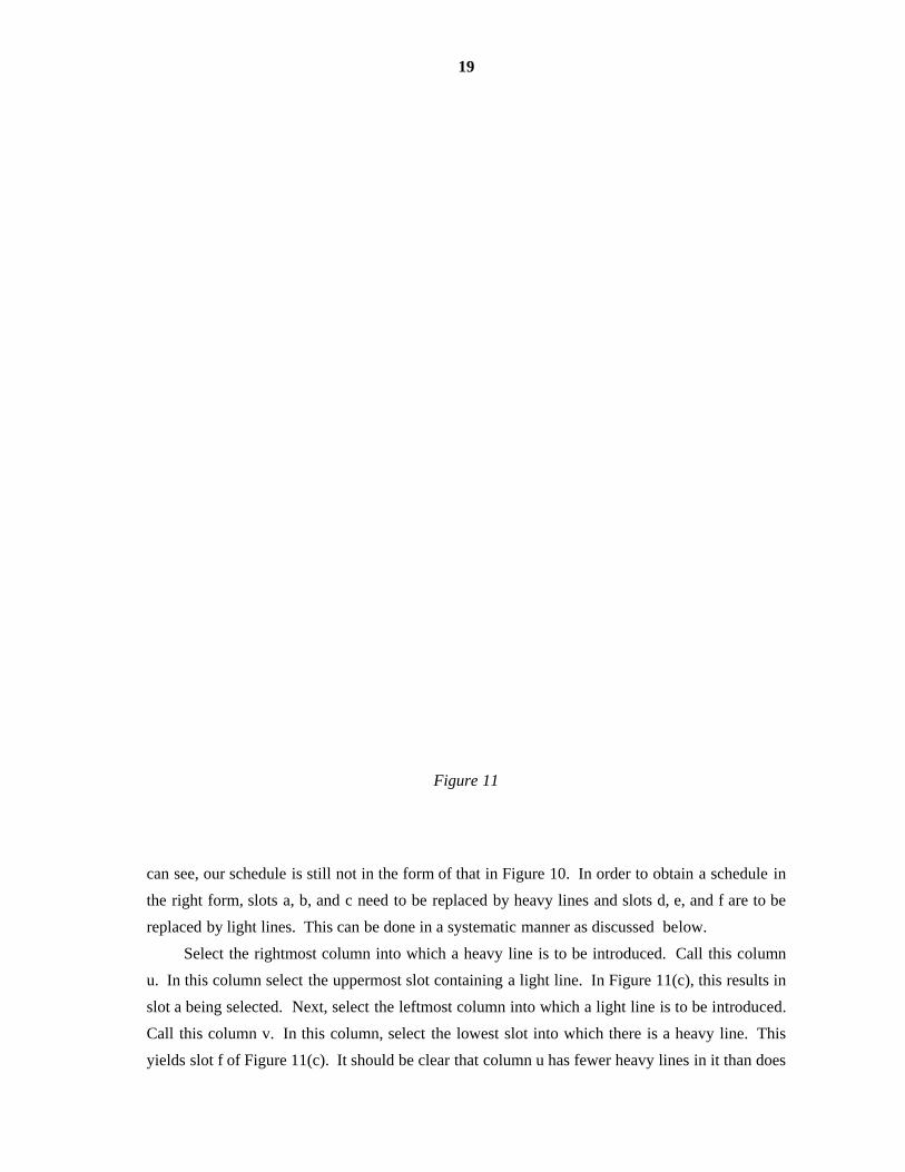
two jobs to be scheduled in the same ∆ interval on any processor. Figure 11(a) shows a possible

configuration for S. The heavy lines represent jobs in R; the light lines represent either jobs in T

or idle times.

First, we shift the heavy lines in each ∆ interval to the top of the ∆ interval. This results in

the light lines moving downwards (but remaining on the A processors). The result is the

schedule of Figure 11(b). This shifting preserves feasibility as the heavy lines move up to pro-

cessors with at least as much memory capacity. The light lines represent jobs in T and these can

be processed on any of the processors in A. In addition, all procesors in A have the same speed.

So, the amount of processing done in a ∆ interval is the same for all procesors in A.

The next transformation is to permute the ∆ intervals so that the number of heavy lines in

each interval is nonincreasing , left to right. This results in the schedule of Figure 11(c). As we

-- --

19

Figure 11

can see, our schedule is still not in the form of that in Figure 10. In order to obtain a schedule in

the right form, slots a, b, and c need to be replaced by heavy lines and slots d, e, and f are to be

replaced by light lines. This can be done in a systematic manner as discussed below.

Select the rightmost column into which a heavy line is to be introduced. Call this column

u. In this column select the uppermost slot containing a light line. In Figure 11(c), this results in

slot a being selected. Next, select the leftmost column into which a light line is to be introduced.

Call this column v. In this column, select the lowest slot into which there is a heavy line. This

yields slot f of Figure 11(c). It should be clear that column u has fewer heavy lines in it than does

-- --

20

column v. Hence, at least one of the heavy lines in v represents a job not scheduled in column u.

We shall select one such heavy line to be moved into column u. This selection is done by first

lining up heavy lines representing jobs common to u and v.

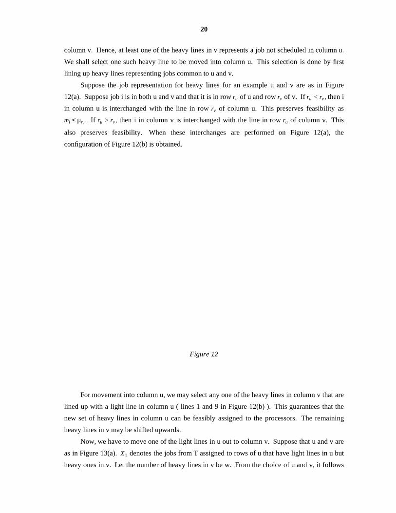
Suppose the job representation for heavy lines for an example u and v are as in Figure

12(a). Suppose job i is in both u and v and that it is in row ru of u and row rv of v. If ru < rv, then i

in column u is interchanged with the line in row rv of column u. This preserves feasibility as

mi ≤ µrv. If ru > rv, then i in column v is interchanged with the line in row ru of column v. This

also preserves feasibility. When these interchanges are performed on Figure 12(a), the

configuration of Figure 12(b) is obtained.

Figure 12

For movement into column u, we may select any one of the heavy lines in column v that are

lined up with a light line in column u ( lines 1 and 9 in Figure 12(b) ). This guarantees that the

new set of heavy lines in column u can be feasibly assigned to the processors. The remaining

heavy lines in v may be shifted upwards.

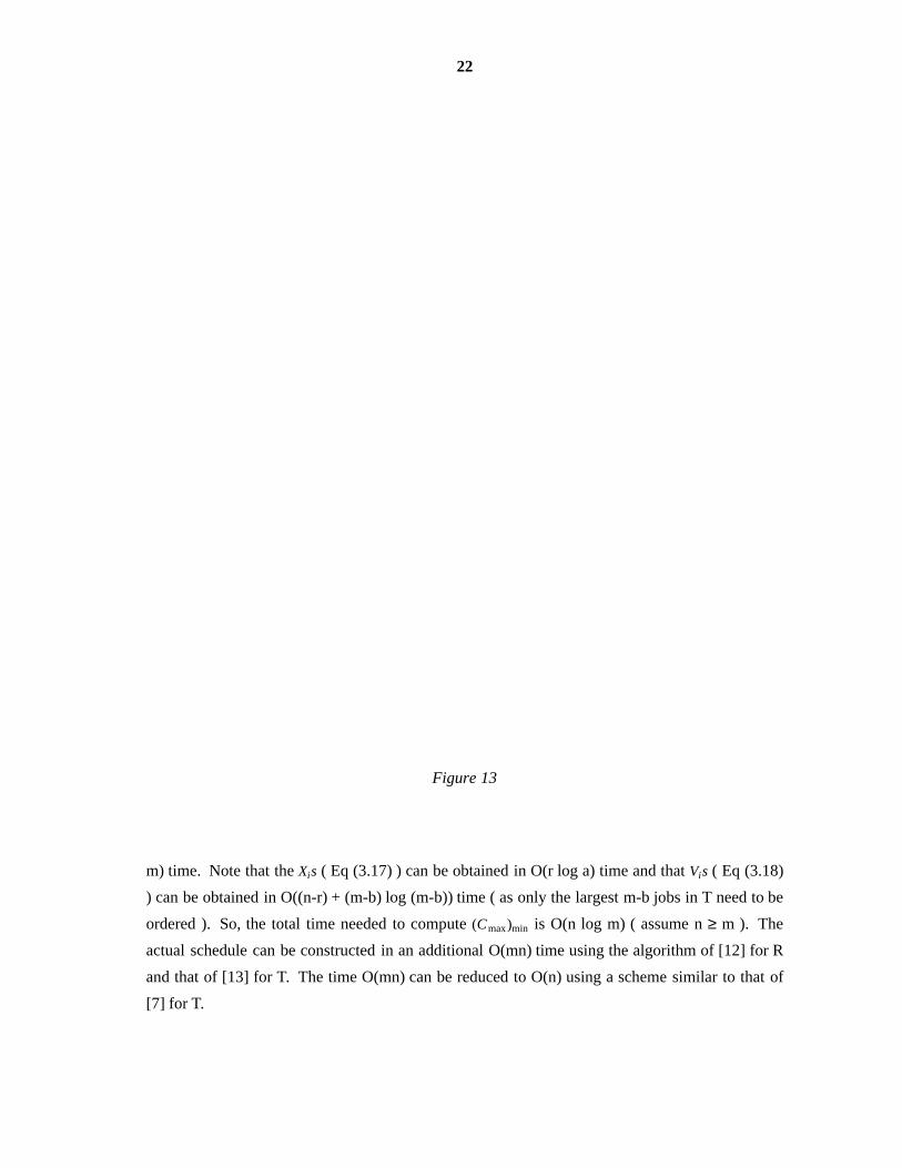
Now, we have to move one of the light lines in u out to column v. Suppose that u and v are

as in Figure 13(a). X1 denotes the jobs from T assigned to rows of u that have light lines in u but

heavy ones in v. Let the number of heavy lines in v be w. From the choice of u and v, it follows

-- --

21

that | X1 | = z ≥ 1. If X1 contains a job that has not been scheduled in column v, then this job may

be selected for movement into column v. Otherwise, permute processors w+1, ..., m so that the

set of jobs scheduled in column v on processors w+1, w+2, ..., w+z is X1. Let X2 denote the set of

jobs scheduled in u on processors w+1, ..., w+z. If every job in X2 is scheduled in column v, then

permute processors w+z+1, ..., m so that the set of jobs scheduled on w+z+1, ..., w+2z in column

v is X2. This permuting of processors is continued until we have an Xk such that at least one job

in Xk is not scheduled in column v. Such an Xk exists as u has fewer heavy lines than does v. Let

x 0 ε Xk be such that x 0 is not scheduled in v. Interchange x 0 with the job, x 1, scheduled on the

same processor in v. Clearly, x 1 ε Xk −1. Hence x 1 is scheduled in u on one of the processors w +

(k-3)z + j, 1 ≤ j ≤ z. Let this processor have index q. Interchange the assignment of x 1 on proces-

sor q column u with that of the job, x 2, in column v of q. Now, x 2 ε Xk −2 and x 2 is scheduled on q,

in column u for some q, q ε { w+(k−4)z +j | 1 ≤ j ≤ z}. We may continue interchanges in this way

until we determine xk −1 ε X1 that needs to be moved out of X1 from column u. This xk −1 is to be

moved into the last heavy line spot in column v.

By repeating the interchange process described above a finite number of times, the

configuration of Figure 11(c) can be transformed into the form of Figure 10. Having established

this result, we see that we need concern ourselves only with schedules in which jobs in R are

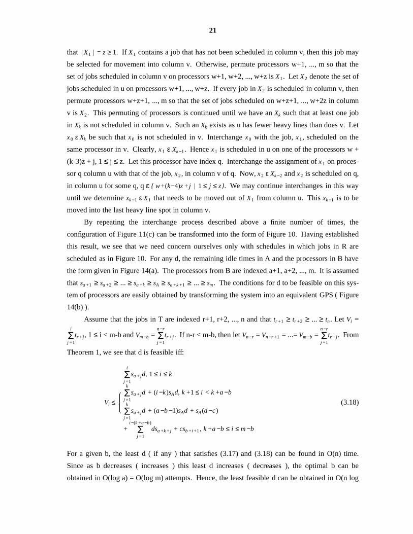
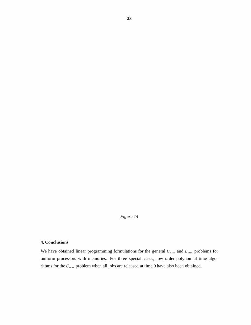
scheduled as in Figure 10. For any d, the remaining idle times in A and the processors in B have

the form given in Figure 14(a). The processors from B are indexed a+1, a+2, ..., m. It is assumed

that sa +1 ≥ sa +2 ≥ ... ≥ sa +k ≥ sA ≥ sa +k +1 ≥ ... ≥ sm. The conditions for d to be feasible on this sys-

tem of processors are easily obtained by transforming the system into an equivalent GPS ( Figure

14(b) ).

Assume that the jobs in T are indexed r+1, r+2, ..., n and that tr +1 ≥ tr +2 ≥ ... ≥ tn . Let Vi =

j =1Σ

i

tr +j, 1 ≤ i < m-b and Vm −b =j =1Σn −r

tr +j. If n-r < m-b, then let Vn −r = Vn −r +1 = ...= Vm −b =j=1Σn −r

tr +j. From

Theorem 1, we see that d is feasible iff:

Vi ≤

�� �

+ j =1Σ

i−(k +a −b)

dsa +k +j + csb +i+1 , k +a −b ≤ i ≤ m −b

j=1Σk

sa +jd + (a −b −1)sAd + sA(d −c)

j=1Σk

sa +jd + (i −k)sAd, k +1 ≤ i < k +a −b

j=1Σ

i

sa +jd, 1 ≤ i ≤ k

(3.18)

For a given b, the least d ( if any ) that satisfies (3.17) and (3.18) can be found in O(n) time.

Since as b decreases ( increases ) this least d increases ( decreases ), the optimal b can be

obtained in O(log a) = O(log m) attempts. Hence, the least feasible d can be obtained in O(n log

-- --

22

Figure 13

m) time. Note that the Xis ( Eq (3.17) ) can be obtained in O(r log a) time and that Vis ( Eq (3.18)

) can be obtained in O((n-r) + (m-b) log (m-b)) time ( as only the largest m-b jobs in T need to be

ordered ). So, the total time needed to compute (Cmax)min is O(n log m) ( assume n ≥ m ). The

actual schedule can be constructed in an additional O(mn) time using the algorithm of [12] for R

and that of [13] for T. The time O(mn) can be reduced to O(n) using a scheme similar to that of

[7] for T.

-- --

23

Figure 14

4. Conclusions

We have obtained linear programming formulations for the general Cmax and Lmax problems for

uniform processors with memories. For three special cases, low order polynomial time algo-

rithms for the Cmax problem when all jobs are released at time 0 have also been obtained.

-- --

24

References

1. G. Dantzig, "Khachian’s algorithm: A comment," SIAM News, Vol. 13, No. 5, Oct. 1980.

2. P. Gacs and L. Lovasz, "Khachian’s algorithm for linear programming," Math. Prog. Study,

Vol. 14, 1981, PP. 61-68.

3. M. R. Garey and D. S. Johnson, "Computers and intractability, a guide to the theory of NP-

Completeness," W. H. Freeman and Co., San Francisco, 1979.

4. S. Gass, "Linear programming," McGraw Hill Book Co., New York, 1969.

5. T. Gonzalez and D. Johnson, "A new algorithm for preemptive scheduling of trees," JACM,

Vol. 27, No. 2, 1980, pp. 287-312.

6. T. Gonzalez and S. Sahni, "Open shop scheduling to minimize finish time," JACM, Vol. 23,

No. 4, 1976, PP. 665-679.

7. T. Gonzalez and S. Sahni, "Preemptive scheduling of uniform processor systems," JACM,

Vol. 25, 1978, PP. 92-101.

8. D. G. Kafura and V. Y. Shen, "Task scheduling on a multiprocessor system with indepen-

dent memories," SICOMP, Vol. 6, No. 1, 1977, PP. 167-187.

9. L. G. Khachian, "A polynomial algorithm in linear programming," Soviet Math. Dokl., Vol.

20, No. 1, 1979, PP. 191-194.

10. V. Klee and G. L. Minty, "How good is the simplex algorithm?" in O. Shisha ( ed. ) Inequal-

ities III, Academic Press, New York, 1972, PP. 159-175.

11. T. H. Lai and S. Sahni, "Preemptive scheduling of a multiprocessor system with memories

to minimize Lmax," Report No. 81-20, Computer Science Dept., Univ. of Minnesota, Min-

neapolis, 1981.

12. R. McNaughton, "Scheduling with deadlines and loss functions," Manag-Sci, 12, 7, 1959.

13. S. Sahni and Y. Cho, "Scheduling independent tasks with due times on a uniform processor

system," JACM, Vol. 27, No. 3, 1980, PP. 550-563.

14. S. Sahni and Y. Cho, "Nearly on line scheduling of a uniform processor system with release

times," SICOMP, Vol. 8, No. 2, 1979, pp. 275-285.

-- --