Embed Size (px)
Citation preview


Preface In June of 2003 the Minnesota Legislature adopted a requirement for an Independent Study of Intermittent Resources, which evaluates the impacts of over 825 MW of wind power on the NSP systeml. The Public Utilities Commission requested that the Department of Commerce take responsibility for oversight of the Study with the understanding that the Office of the Reliability Administrator would represent the Departmentz.
After the conclusion of the 2003 Legislative session a thorough and complete research of the current status and understanding of integrating wind power into electric power systems, including a comprehensive literature search, was completed. A broad-based workgroup was assembled to guide the initial development of the Study. This group included representatives of Xcel Energy, Minnesota municipal utilities, Minnesota cooperative utilities, the Minnesota Chamber of Commerce, the American Wind Energy Association, Minnesota environmental organizations, the U.S Department of Energy / National Renewable Energy Laboratory, and the Department of Commerce.
Members of that workgroup included:
Jim Alders
Rory Artig
Bill Blazar
Laura Bordelon
Jim Caldwell
Bob Cupit
Chris Davis
Bill Grant
Clair Moeller
Michael Noble
Brian Parsons
Judy Poferl
Larry Schedin
Matt Schuerger
Craig Turner
Greg Woodworth
Ken Wolf
Xcel Energy
Minnesota Department of Commerce
Minnesota Chamber of Commerce
Minnesota Chamber of Commerce
American Wind Energy Association
Minnesota Department of Commerce
Minnesota Department of Commerce
Izaak Walton League of America
Xcel Energy
ME3
National Renewable Energy Laboratory
Xcel Energy
Reliant Energy Integration Services
Energy Systems Consulting Services
Dakota Electric Association
Rochester Public Utilities
Minnesota Department of Commerce
' Minnesota Laws 2003, 1" Special Session, Chapter 11, Article 2, Section 21. MN PUC Docket No. E-002lCI-03-870, Order Requiring Engineering Study
Page 2 C O R P O R A T I O N
. : * 45 2857
* . i , , ,

The workgroup met several times to develop the Statement of Work for the study. Xcel Energy competitively bid the study and contracted with the successful bidder, a team lead by EnerNex Corporation. ,,
This study is a sigruficant advance in the science and understanding of the impacts of the variability of wind power on power system operation in the Midwest. For example, the application of sophisticated, science-based atmospheric models to accurately characterize the variability of Midwest wind generation is a vast improvement over previous methods.
The study benefited from extensive expert guidance and review by a Technical Review C o d t t e e P C > - Thank you to all of the participants in the TRC, which included:
Jim Alders Xcel Energy
Steve Beuning Xcel Energy
Laura Bordelon
Jim Caldwell
Bob Cupit
Ed DeMeo
' .John Donatell
David Duebner
Bill Grant
Walt Grivna
Mark Haller
Rick Halet
Larry Hartman
Mike Jacobs
Minnesota Chamber of Commerce
American Wind Energy Association/PPM Energy
Minnesota Department of Commerce
Utility Wind Interest Group/ Renewable Energy Consulting Services, Inc.
Xcel Energy
idw west Independent System Operator
Izaak Walton League
Xcel Energy
American Wind Energy Association/ Haller Wind Consulting
Xcel Energy
Minnesota Environmental Quality Board
American Wind Energy Association
Stephen Jones Xcel Energy
Mark McGree Xcel Energy
Mike McMullen Xcel Energy
Michael MiUigan National Renewable Energy Laboratory
Michael Noble. Minnesotans for an Energy Efficient Economy
Dale Osborn Midwest Independent System Operator
Brian Parsons National Renewable Energy Laboratory
Lisa Peterson Xcel Energy
Rick Peterson Xcel Energy
Greg Pieper Xcel Energy
Larry Schedin Technical Advisor to the MN DOC

Matt Schuerger Technical Advisor to the MN DOC
Steve Wilson Xcel Energy
Ken Wolf Minnesota Department of Commerce
The aggressive schedule for completion of this study prevented investigation of several critical next steps. The study outlines several important next steps needed to develop effective solutions to mitigate these impacts including improved strategies and practices for unit commitment and scheduling as well as improved forecasting and markets.
Ken Wolf
Reliability Administrator Minnesota Department of Commerce
E n ~ t - N e k Page 4 C O R ~ O R A ~ I O N $ t; f: -J ,, 2959

Project Team
EnerNex Corporation Robert M. Zavadil - Project Manager
Jack King
Leo Xiadong
WindLogics Mark Ahlstrom
Dr. Bruce Lee
Dr. Dennis Moon
Dr. Cathy Finley
Lee Alnes
Arreva T&D Dr. Lawrence Jones
Fabrice Hudry
Mark Monstream
Stephen Lai
NexGen Energy LLC J. Charles Smith
Page 5 , r < 3 R s ~ O R A T I O N .. . .

Contents
............................................................................................................................. Project Summary 15
Introduction ........................................................................................ ............................................. 15 ........................................................................................... Overview of Utility System Operations 15
Characteristics of Wind Generation ............................................................................................. 17 . wind Generation and Long-Term Power System Reliability ....................................................... 18
.................................................................................................................... Objectives of this Study 19
Organization of Documentation ................................................................................................... 20 Task 1: Characterizing the Nature of Wind Power Variability in the Midwest . Overview and Results ........................................................................................................................................ 20
Task 2: Develop Xcel Energy System Model for 2010 Study Year . Overview and Results .... 24 Task 3: Evaluation of Wind Generation Reliability Impacts . Overview and Results .............. 26 Task 4: Evaluation of Wind Generation Integration Costs on the operating Time Frame . Overview and Results ....................................................................................................................... 29
Regulation ....................................................................................................................................... 30
....... Unit Commitment and Scheduling - Hourly Impacts ; ........................................................ 32
..................................................................................... Load Following and Intra-hourly Effects 34
Conclusions ........................................................................................................................................ 38 Task 1: Wind Resource Characterization ..................................................................................... 41
Task Description ................................................................................................... ........................... 41 Introduction ....................................................................................................................................... 41 Wind Resource Characterization ................................................................................................... 42
Controlling Meteorology for the Upper Midwest ...................................................................... 42 Modeling Methodology and Utilization of Weather Archives ................................................. 44 Normalization of Model Wind Data with Long-Term Reanalysis Database .......................... 45
Validation of Modeled Winds ...................................................................................................... 46 Description of Multi-Scale Aspects of Modeled Wind Variability ........................................... 46 NREL Database. Comparison Methodology. and Model Output Loss Factor Adjustment47
Validation for 2003 . Monthly Comparison Time Series and Statistics ................................... 47 ....................... ........................................................... Task 2: Xcel System Model Development 54
Task Description ................................................................................................................................. 54 .............................................................................................................. Wind Generation Scenario 54
................................................................ Turbine Technology and Power Curve Assumptions 55
......................................................... Deployment of Turbine Technologies in Study Scenario 57
E n e r N e k Page 6 C O R P O R A T l O N 2 8 6 1

Development of Wind Generation Profiles ................................................................................ 58
Xcel System Model ........................................................................................................................ 58
Detailed Model Data .................................................................................................................. 59
Generating Unit Characterization ............................................................................................... 59 ................................................................. Historical Performance Data for Xcel-North System 60
Other Data ...................................................................................................................................... 60
Task 3: Reliability Impacts of Wind Generation ............................................................................ 62
Task Description ................................................................................................................................. 62
Description of Modeling Approach ......................................................................................... 62
Model Assumptions ........................................................................................................................... 63
Non-wind Units mapped to MARS data file ............................................................................... 63
Non-wind Units not mapped to MARS data file ........................................................................ 63
Manitoba Hydro Firm Contract Purchases ................................................................................. 63
Other Purchases ............................................................................................................................. 64
Wind Resources .............................................................................................................................. 64
Results ................................................................................................................................................. 65
...................... Results of MAPP Accreditation procedure for Variable Capacity Generation 73
Observations .................................................................................. .......................................... 74
Recommendations ......................................................................................................................... 75
Task 4: Evaluate Wind Integration Operating Cost Impacts ....................................................... 77
Task Description .................................................................... .......................................................... 77
Calculation of Incremental Regulation Requirements ................................................................ 78
Regulation . Background ............................................................................................................... 78
Statistical Analysis of Regulation ............................................................... .................................... 79
Regulation Characteristics of Xcel-NSP System Load ............................................. ................... 81
............................................................................ Characteristics of Proposed Wind Generation 84
............................................................... Calculation of Incremental Regulating Requirements 89
Conclusions ...................................................................................... ............................................... 89 Impact of Wind Generation on Generation Ramping . Hourly Analysis .................................... 91
............................. Analysis of Historical Load Data and Synthesized Wind Generation Data 91
.................................. Assessment of Wind Generation Impacts on Ramping Requirements 102
Unit Commitment and Scheduling with Wind Generation ........................................................ 103
Overview .................................................................... ................................................................. 103
Methodology for Hourly Analysis ................................................................................................ 104
Model Data and Case ......................................... ........................................................................ 106

System Data ............................................................................................................................ 106
Wind Generation and Forecast Data .................................................................................... 106
Rationale for the "Reference" Case ...................................................................................... 108
Case Structure ............................................................................................................................. 109 Assumptions .................................................................................................................................. 109
Supply Resources .................................................................................................................... 109 Transactions . Internal ............................................................................................................ 109 Transactions . External ........................................................................................................... 109
Fuel Costs ................................................................................................................................... 1 1 1
Results ............................................................................................................................................... 111
Notes on the Table: .................................................................................................................... 111
Discussion ...................................................................................................................................... i12
Load Forecast Accuracy Issues .................................................................................................... 116
MISO Market Considerations ......................................................................................................... 119
Intra-Hourly Impacts .................................................................................................................... 123
Background ...................................................................................................................................... 123
Data Analysis ................................................................................................................................... 123
Discussion ............................................................................................................................. ; . 128
Load Following Reserve Impacts .................................................................................................. 131
................................................................................................ Conclusions - Intra-hourly Impact 133
Task 4 - Summary and Conclusions ............................................................................................ 134
Project Retrospective and Recommendations ......................................................................... 137
Observations ..................................................................................................................... .............. 137 Value of Chronological Wind and Load Data for Analysis .................... .; ............................ 137
Variability and Forecast Error ................................................................................................ 137
Methodology and Tools ............................................................................................................. 139 Recommendations for Further Investigation .............................................................................. 139
References ...................................................................................................................................... 143
E n e r N ~ k Page 8 C O R P O R A T I O N

List of Tables
Table 1 : Minnesota Wind Generation Development Scenario . CY2010 ................................. 24
Table 2: Xcel Capacity Resources for 201 0 ................................................................................... 24
Table 3: Computed capacity values for 1500 MW wind generation scenario using MAPP accreditation procedure ....................................................................................... 28
..................................................................................... Table 4: Hourly Integration Cost summary 34
Table 5: Ten-minute Variations in Control Area Demand. with and without Wind Generation ........................................................................................................................... 38
Table 6: County Totals for 1500 MW of Wind Generation in Study ............................................. 54
.................................... Table 7: Wind Generation by County and Turbine Type : ........................ 57
................................................................ Table 8: Xcel-North Project Supply Resources for 201 0 58
Table 9: Wind Generation by County and Turbine Type ............................................................. 64
.......................................................... Table 10: Seasonal Definitions for Wind Generation Model 65
Table 1 1 : MARS Case List and Descriptions ....................................................................................... 65 ................................................................................................... Table 12: ELCC Calculation Results 66
................................................................................................... Table 13: GE-MARS results by week 68
Table 14: Source Data for LOLE Curves of Figure 34 ....................................................................... 70
Table 15: Monthly accreditation of aggregate wind generation in study scenario per MAPP procedure for variable capacity generation ..................................................... 73
Table 16: Monthly accreditation of Buffalo Ridge wind generation using MAPP procedure for variable capacity generation .................................................................................... 74
......... Table 17: Summary of Regulation Statistics for Xcel-NSP System Load. April 12.27. 2004 84
Table 18: Plant Details for NREL Measurement Data ...................................................................... 85
Table 19: Standard Deviation of Regulation Characteristic for NREL Measurement Locations .............................................................................................................................. 88
Table 20: Results of Hourly Analysis for First Annual Data Set (2003 Wind Generation & 2003 Load Scaled to 201 0) ......................................................................................... 113
Table 21 : Results of Hourly Analysis for Second Annual Data Set (2002 Wind Generation & 2002 Load Scaled to 20 10) ......................................................................................... 114
Table 22: Production Cost Comparison for Base. Forecast. and Actual Cases ...................... 115
Table 23: Day-Ahead Peak Load Forecast Accuracy from internal Xcel Study ..................... 116
Table 24: Results of Hourly Cases with Energy Market Assumptions .......................................... 122
.................................................................................. Table 25: Statistics of Ten-Minute Changes 127
Table 26: Extreme System Load Changes . with and without Wind over One Year of Data (-50 K samples) ........................................ ........................................................... 132
EnerNek Page 9 C 0 R . P . 0 R A T I 0 N . r 2" ti . . . . . 2864

List of Figures
~ i ~ u ' r e 1 : MM5 nested grid configuration utilized for study area. The 3 grid run includes 2 inner nested grids to optimize the simulation resolution in the area of greatest interest. The grid spacing is 45, 15 and 5 km for the outer, middle and innermost nests, respectively ............................................................................................................... 21
Figure 2: "Tower" locations on the innermost MM5 model grid where wind speed data and other meteorological data were ca,ptured and archived at ten-minute intervals .......................................................................... :...................................................... 22
Figure 3: Comparison of simulated wind generation data to actual measurements for a group of wind turbines at Lake Benton, MN on the Buffalo Ridge ............................. 22
Figure 4: Frequency distribution of power error as a percent of rated capacity for 6,24 and 48 hour forecasts. Inset table shows the frequency of power errors less than l0,20 and 30 percent of rated capacity for the CLS 6,24 and 48 hour forecasts. .23
Figure 5: Xcel supply resources for 201 0 by type and fuel. .......................................................... 25
Figure 6: Measurements of existing load data used for characterizing expected load in 201 0. Graph shows 72 hours of data collected at 4 second intervals by the Xcel Energy Management System (EMS) ............................................................................. 25
Figure 7: NREL high-resolution measurement data from Lake Benton wind plants and Buffalo Ridge substation. Data show is power production sampled at one second intenials. ................................................................................................................. 26
Figure 8: Results of reliability analysis for various wind generation modeling assumptions ..... 27
Figure 9: Actual load (blue) and hourly trend (red) for one hour ............................................... 30
Figure 10: Typical daily wind generation for Buffalo Ridge plants data sampled at one second intervals for 24 hours ............................................................................................. 31
Figure 1 1 : Block diagram of methodology used for hourly analysis. ............................................ 32
....................................... Figure 12: Wind generation forecast vs. actual for a two week period 33
Figure 13: Weekly time series of ten-minute variations in load and wind generation. ............... 35
Figure 14: Control area net load changes on ten minute intervals with and without wind generation. .......................................................................................................................... 35
Figure 15: Variation at ten-minute increments from daily "trend" pattern, with and without wind generation .................................................................................................................. 36
Figure 1 6: Expanded view of Figure 14. ............................................................................................. 37
Figure 17: Mean winter and summer positions of the upper-tropospheric jet stream. Line width is indicative of jet stream wind speed .................................................................. 43
Figure 18: Typical "storm tracks" that influence the wind resource of the Upper Midwest. The bold Ls represent surface cyclone positions as they move along the track. .... 43
Figure 19: MM5 nested grid configuration utilized for study area. The 3 grid run includes 2 inner nested grids to optimize the simulation resolution in the area of greatest interest. The grid spacing is 45, 15 and 5 km for the outer, middle and innermost nests, respectively. The colors represent the surface elevation respective to each grid. ....................................................................................................................................... 45

Figure 20: Innermost model grid with proxy MM5 tower (data extraction) locations . The color spectrum represents surface elevation ................................................................. 46
Figure 21 : January (top) and February (bottom) power time series for MM5 Tower 24 and the Delta Sector . Mean error (ME). mean absolute error (MAE) and correlation coefficient are shown in the upper right box ................................................................. 48
Figure 22 March (top) and April (bottom) power time series for MM5 Tower 24 and the Delta Sector . Mean error (ME). mean absolute error (MAE) and correlation coefficient are shown in the upper right box ................................................................. 49
Figure 23: May (top) and June (bottom) power time series for MM5 Tower 24 and the Delta Sector . Mean error (ME). mean absolute error (MAE) and correlation coefficient are shown in the upper right box ................................................................. 50
Figure 24: July (top) and August (bottom) power time series for MM5 Tower 24 and the Delta Sector . Mean error (ME). mean absolute error (MAE) and correlation coefficient are shown in the upper right box ................................................................ 51
Figure 25: September (top) and October (bottom) power time series for MM5 Tower 24 and the Delta Sector . Mean error (ME). mean absolute error (MAE) and correlation coefficient are shown in the upper right box ............................................ 52
Figure 26: November (top) and December (bottom) power time series for MM5 Tower 24 and the Delta Sector . Mean error (ME). mean absolute error (MAE) and correlation coefficient are shown in the upper right box ............................................ 53
Figure 27: Wind generation scenario ................................................................................................. 55 Figure 28: Power. torque. and generator speed relationships for Enron 250 750 kW wind
................................................................................................................................... turbine 56
Figure 29: Power curve for new near-term projects in study scenario .......................................... 56
Figure 30: Power curve for longer-term projects in study scenario; meant to serve as a proxy for "low wind speed" turbine technology ........................................................... 57
................................................ Figure 31 : Xcel-North generation resources for 201 0 by fuel type 59
Figure 32: Sample of high-resolution (4 second) load data from Xcel EMS for three days in April. 2004 ............................................................................................................................. 60
Figure 33: Illustration of High-resolution (1 second) wind plant measurement data from NREL monitoring program .................................................................................................. 61
Figure 34: LOLE and ELCC results ........................................................................................................ 66 Figure 35: Effects of wind generation by county on LOLE .............................................................. 71
Figure 36: Sample wind generation time series generated by GE-MARS ..................................... 72
Figure 37: Instantaneous system load at 4 second resolution and load trend ............................ 79 .
........... Figure 38: Equations for separating regulation and load following from load (from[l]) 80
........................................... Figure 39: Regulation characteristics for raw load data of Figure 37 80
Figure 40: High-resolution load data archived from Xcel-NSP EMS ............................................... 82
Figure 41 : Raw load data and trend with 20 minute time-averaging period ............................. 83
......................................................................... Figure 42: Regulation characteristic from Figure 41 83
............................................... Figure 43: Distribution of regulation variations for April 12-1 4. 2004 84
E n t r N t k Page 11 C ~ ~ P O R A T I O N
? c-: t; .. 2866

Figure 44: Portion of NREL measurement data showing per-unitized output at each monitoring location .................................................................. : ..................................... i ... 86
Figure 45: Expanded view of Figure 44 beginning at Hour 5 .......................................................... 86
Figure 46: Trend characteristic extracted from raw data of Figure 44 with a 20 minute time averaging period ................................................................................................................ 87
Figure 47: Variation of the standard deviation of the regulation characteristic for each of nine sample days by number of turbines comprising measurement group ............. 88
Figure 48: System Load and Wind Generation data sets used in assessment of ramping requirements ........................................................................................................................ 92
Figure 49: Expanded view of Figure 48 beginning'on Day 100 ................................................... 93
Fig'ure 50: Distribution of hourly changes in system load without wind forthree year .................................................................................................................................. sample 94
Figure 51: Distribution of hourly changes in system load with wind for three year sample ....... 94
Figure 52: Control area hourly load (no wind) changes for hours ending 3. 6; 9. 12. 15. 18 . 21. & 24 ................................................................................................................................. 96
Figure 53: Control area hourly load (with wind) changes for hours ending 3.6.9. 12.15.18.
Figure 54: Control area hourly load changes for hours ending 6. 12 &18 . Load only (red)' and with wind (blue) .......................................................................................................... 98
Figure 55: Average ramping requirements with and without wind for each hour of the day. by season ............................................................................................................................. 99
Figure 56: Standard deviation of ramping requirements with and without wind generation. ............................................................................................ by hour of day and season 100
Figure 57: Ramping requirements with and without wind generation for selected hours during the winter season ................................................................................................ 101
Figure 58: Ramping requirement with and without wind generation for selected hours .
during spring ..................................................................................................................... 101
Figure 59: Ramping requirement with and without wind generation for selected hours during summer ........................................................................................................... 102
Figure 60: Ramping requirement with and without wind generation for selected hours during fall ........................................................................................................................... 102
Figure 61 : Overview of methodology for hourly analysis ............................................................. 105
Figure 62: Actual and'forecast wind generation for two weeks in March. 2003 ...................... 107
Figure 63: Actual and forecast wind generation for two weeks in July. 2003 ........................... 108
Figure 64: Forecast error statistics for 2003 wind generation time series ................................... 108
Figure 65: Typical Xcel Energy purchases and sales for Spring '04 ......................................... 110
Figure 66: Assumed transactions for 201 0 hourly analysis ............................................................ 110
Figure 67: Variable components of 2010 daily purchases and sales (excludes Manitoba Hydro 5x1 6 contract for 500 MW and forced sale of 250 MW) ................................ 111
Figure 68: Load forecast series developed with Xcel load forecast accuracy statistics ....... 117

Figure 69: Distribution of hourly load forecast errors for the load forecast synthesis methods . 118
Figure 70: Forecast error statistics for 2003 wind generation time series ................................... 118
Figure 71 : Hourly forecast error distribution for load only and load with wind ......................... 119
Figure 72: Day-ahead scheduled and actual transactions for January market simulation case: ................................................................................................................................ 121
Figure 73: Assumed hour-ahead transactions for the January case ......................................... 121
Figure 74: High resolution load and wind generation data ......................................................... 123
......................................................... Figure 75: Changes in system load at ten minute intervals 124
Figure 76: Ten-minute changes in wind generation from synthesized high-resolution wind .............................................................................................................. generation data 124
Figure 77: System load and aggregate wind generation changes for a one week period . 125
Figure 78: Distribution of 10 minute changes in system load ..................................................... 125
Figure 79: Distribution of 10 minute changes in aggregate wind generation ......................... 126
Figure 80: Control area net load changes on ten minute intervals with and without wind generation ...................................................................................................................... 126
........................................................................................... Figure 81 : Expanded view of 'Figure 80 127
Figure 82: 12-hour load time series showing high-resolution data (red). hourly trend (blue). and hourly average value (magenta) ......................................................................... 128
Figure 83: Distribution of ten-minute deviations in system load from hourly trend curve. with (red) and without wind generation (blue) ................................................................. 129 .
........................................................................................... Figure 84: Expanded view of Figure 83 130
Figure 85: Ten-minute system load changes with (red) and without (blue) wind ................... generation .................................................................................................... : 132
Figure 86: Empirical relationship between monthly wind energy forecast error and ........................... production cost difference between actual and forecast cases 138
Figure 87: Empirical relationship between monthly energy forecast error and a) production cost difference'between actual and forecast case (black); and b) actual and
..................................................................................................... base case (magenta) 138
E n e r N e k Page 13 C:O R P-'o$ k A T 1 0 N . .

E n e r N e k page 14 C O R P O R A T I O N

Introduction In 2003, the Minnesota Legislature adopted a requirement for an Independent Study of Intermittent Resources to evaluate the impacts of over 825 MW of wind power on the Xcel Energy system. The Minnesota Public Utilities Commission requested that the office of the Reliability Administrator of the Minnesota Department of Commerce take responsibility for the study and its scope and administration. Through a competitive bidding process, the study was commissioned in January of 2004. Results of that study are reported here.
Xcel Energy, formed by the merger of Denver-based New Centuries Energies and Minneapolis-based Northern States Power Company, is the fourth-largest combination electricity and natural gas energy company in the United States. Xcel Energy serves over 1.4 million electric customers in the states of Minnesota, Wisconsin, North Dakota, South Dakota and Michigan. Their peak demand in this region is approximately 9,000 MW in 2003 and projected to rise to approximately 10,000 MW by 2010.
In 2003, the Xcel Energy operating area in Minnesota, Wisconsin, and parts of the Dakotas had about 470 MW of wind power under contract, including about 300 MW operating, in southwestern Minnesota. An additional 450 MW of wind power has been awarded through the 2001 AU Source Bid process. Minnesota legislation could result in a total of 1,450 to 1,750 MW of wind power serving the NSP system by 2010 and 1,950 to 2,250 MW by 2015.
An earlier study commissioned by Xcel Energy and the Utility Wind Interest Group (UWIG, www.uwi~.orq) - estimated that the approximately 300 MW of wind generation in Xcel Energy's control area in Minnesota at that time resulted in additional annual costs to Xcel of $1.85 for each megawatt-hour (MWH) of wind energy delivered to the system. While for some time there had been recognition and consensus that the unique characteristics of wind generation likely would have some technical and financial impacts on the utility system, this study was the first attempt at a formal quantification for an actual utility control area.
,
The study looked at the "operating1' time frame, which consists primarily of those activities required to ensure that there wiU be adequate electric energy supply to meet the projected demand over the coming hours and days, that the system is operated at all times so as not to compromise security or reliability, and that the demand be met at the lowest possible cost.
The study reported on here takes a similar perspective. The scenario evaluated, however, is dramatically different. Instead of 300 MW of wind generation confined to relatively small parts of two adjacent counties, a potential future development of 1500 MW of wind generation spread out over hundreds of square miles is considered. In addition, the wind generation central to the previous study was well characterized through existing monitoring projects and measurements at all of the time scales of interest, making questions about how wind generation would appear to the Xcel system operators relatively simple to address. In this study, developing a characterization of how large, geographically-diverse wind plants would appear in the aggregate to the system operators was one early and major challenge.
To better understand the study scope, its specific challenges, and the results, some background on utility system operations and the characteristics of wind generation is helpful.
Ovetview of Utility System Operations Interconnected power systems are large and extremely complex machines, consisting of thousands of individual elements. The mechanisms responsible for their control must continually adjust the supply of electric energy to meet the combined and ever-changing electric demand of the system's
E n e r N k Page 15 C ' O R q Q R A T I O N ' ? :-. -; 2870

users. There are a host of constraints and objectives that govern how this is done. For example, the system must operate with very high reliability and provide electric energy at the lowest possible cost. Limitations of individual network elements -generators, transmissionlines, substations - must be honored at all times. The capabilities of each of these elements must be utilized in a fashion to provide the required high levels of performance and reliability at the lowest overall cost.
Operating the power system, then, involves much more than adjusting the combined output of the supply resources to meet the load. Maintaining reliability and acceptable performance, for example, requires that operators:
Keep the voltage at each node (a point where two or more system elements - lines, ~ansformers, loads, generators, etc. - connect) of the system within prescribed limits;
Regulate the system frequency (the steady electrical speed at which all generators in the system are rotating) of the system to keep all generating units in synchronism;
Maintain the system in a state where it able to withstand and recover from unplanned failures or losses of major elements
The activities and functions necessary for maintaining system performance and reliability and minimizing costs are generally classified as "ancillary services." While there is no universal agreement on the number or specific definition of these services, the following items adequately encompass the range of technicd aspects that must be considered for reliable operation of the system:
Voltage regulation and VAR dispatch - deploying of devices capable of generating reactive power to manage voltages at all points in the network;
Regulation - the process of maintaining system frequency by adjusting cer& generating units in response to fast fluctuations in the total system load;
Load following - moving generation up (in the morning) or down (late in the day) in response to the daily load patterns;
Frequency-responding spinning reserve - maintaining an adequate supply of generating capacity (usually on-line, synchronized to the grid) that is able to quickly respond to the loss of a major transmission network element or another generating unit; ,
Supplemental Reserve - managing an additional back-up supply of generating capacity that can be brought on line relatively quickly to serve load in case of the unplanned loss of signifcant operating generation or a major transmission element.
The frequency of the system and the voltages at each node are the fundamental performance indices for the system. High interconnected power system reliability is a consequence of maintaining the system in a secure state - a state where the loss of any element will not lead to cascading outages of other equipment - at all times.
The electric power system in the United States (contiguous 48 states) is comprised of three interconnected networks: the Eastern Interconnection (most of the states East of the Rocky Mountains), the Western Interconnection (Rocky Mountain States west to the Pacific Ocean), and ERCOT (most of Texas). Within the Eastern and Western interconnections, dozens of individual "control" areas coordinate their activities to maintain reliability and conduct transactions of electric energy with each other. A number of these individual control areas are members of Regional Transmission Organizations (RTOs), which oversee and coordinate activities across a number of control areas for the purposes of maintaining the security of the interconnected power system and implementing wholesale power markets.
'A control area consists of generators, loads, and defined and monitored transmission ties to neighboring areas. Each control area must assist the larger interconnection with maintaining

frequency at 60 Hz, and balance load, generation, out-of-area purchases and sales on a continuous basis. In addition, a prescribed amount of backup or reserve capacity (generation that is unused but available within a certain amount of time) must be maintained at all times as protection against unplanned failure or outage of equipment.
To accomplish the objectives of minimizing costs and ensuring system performance and reliability over the short term (hours to weeks), the activities that go on in each control area consist of:
Developing plans and schedules for meeting the forecast load over the coming days, weeks, and possibly months, considering all technical constraints, contractual obligations, and financial objectives;
Monitoring the operation of the control area in real time and making adjustments when the actual conditions - load levels, status of generating units, etc. - deviate from those that were forecast.
A number of tools and systems are employed to assist in these activities. Developing plans and schedules involves evaluating a very large number of possibilities for the deployment of the available generating resources. A major objective here is to utilize the supply resources so that all obligations are met and the total cost to serve the projected load is minimized. With a large number of individual generating units with many different operational characteristics and constraints, fuel types, efficiencies, and other supply options such as energy purchases from other control areas, software tools must be employed to develop optimal plans and schedules. These tools assist operators in making decisions to "commit" generating units for operation, since many units cannot realistically be stopped or started at wiU. They are also used to develop schedules for the next day or days that will result in minimum costs if adhered to and if the load forecasts are accurate.
The Energy Management System (EMS) is the technical core of modem control areas. It consists of hardware, software, communications, and telemetry to monitor the real-time performance of the control area and make adjustments to generating unit and other network components to achieve operating performance objectives. A number of these adjustments happen very quickly without the intervention of human operators. Others, however, are made in response to decisions by individuals charged with monitoring the performance of the system.
The nature of control area operations in real-time or in planning for the hours and days ahead is such that increased knowledge of what will happen correlates strongly to better strategies for managing the system. Much of this process is already based on predictions of uncertain quantities. Hour-by- hour forecasts of load for the next day or several days, for example, are critical inputs to the process of deploying electric generating units and scheduling their operation. While it is recognized that load forecasts for future periods can never be 100% accurate, they nonetheless are the foundation for all of the procedures and process for operating the power system. Increasingly sophisticated load forecasting techniques and decades of experience in applying this information have done much to lessen the effects of the inherent uncertainty
Characteristics of Wind Generation The nature of its "fuel" supply distinguishes wind generation from more traditional means for producing electric energy. The electric power output of a wind turbine depends on the speed of the wind passing over its blades. The effective speed (since the wind speed across the swept area of the wind turbine rotor is not necessarily uniform) of this moving air stream exhibits variability on a wide range of time scales - from seconds to hours, days, and seasons. Terrain, topography, other nearby turbines, local and regional weather patterns, and seasonal and annual climate variations are just a few of the factors that can influence the electrical output variability of a wind turbine generator.

It should be noted that variability in output is not confined only to wind generation. Hydro plants, for example, depend on water storage that can vary from year to year or even seasonally. Generators that utilize natural gas as a fuel can be subject to supply disruptions or storage limitations. Cogeneration plants may vary their electric power production in response to demands for steam rather than the wishes of the power system operators. That said, the effects of the variable fuel supply are likely more sigruhcant for wind generation, if only because the experience with these plants accumulated thus far is so limited.
An individual turbine is negligibly small with respect to the load and other supply resources in the control area, so the aggregate performance of a large number of turbines is what is of primary interest with respect to impacts on the transmission grid and system operations. Large wind generation facilities that connect directly to the transmission grid employ large numbers of individual wind turbine generators, with the total nameplate generation on par with other more conventional plants. Individual wind turbine generators that comprise a wind plant are usually spread out over a sigruficant geographical area. This has the effect of exposing each turbine to a slightly different fuel supply. This spatial diversity has the beneficial effect of "smoothing out" some of the variations in electrical output. The benefits of spatial diversity are also apparent on larger geographical scales, as the combined output of multiple wind plants will be less variable (as a percentage of total output) than for each plant individually.
Another aspect of wind generation, which applies to conventional generation but to a much smaller degree, is the ability to predict with reasonable confidence what the output level will be at some time in the future. Conventional plants, for example, cannot be counted on with 100% confidence to produce their rated output at some coming hour since mechanical failures or other circumstances may limit their output to a lower level or even result in the plant being taken out of service. The probability that this will occur, however, is low enough that such an occurrence is often discounted or completely ignored by power system operators in short-term planning activities.
Because wind generation is driven by the same physical phenomena that control the weather, the uncertainty associated with a prediction of generation level at some future hour, even maybe the next hour, is sigruficant. In addition, the expected accuracy of any prediction will degrade as the time horizon is extended, such that a prediction for the next hour will almost always be more accurate than a prediction for the same hour tomorrow.
The combination of production variability and relatively high uncertainty of prediction makes it difficult, at present, to "fit" wind generation into established practices and methodologies for power system operations and short-term pl-g and scheduling. These practices, and even emerging concepts such as how- and day-ahead competitive markets, have a necessary bias toward "capacity" - because of system security and reliability concerns so fundamental to power system operation - with energy a secondary consideration. Wind generation is a clean, increasingly inexpensive, and stable supply of electric energy. The challenge going forward is to better understand how wind energy as a supply resource interacts with other types of electric generation and how it can be exploited to maximize benefits, in spite its unique characteristics.
Wind Generation and Long-Term Power System Reliability In longer term planning of electric power systems, overall reliability is often gauged in terms of the probability that the planned generation capacity will be insufficient to meet the projected system demand. This question is important from the planning perspective because it is recognized that even conventional electric generating plants and units are not completely reliable - there is s h e probability that in a given future hour capacity from the unit would be unavailable or limited in capability due to a forced outage - i.e. mechanical failure. This probability of not being able to meet the load demand exists even if the instalIed capacity in the control area exceeds the peak projected load.
Page 18 C O R P O R A T I O N
F 't
.% % L

In this sense, conventional generating units are similar to wind plants. For conventional units, the probability that the rated output would not be available is rather low, while for wind plants the probability could be quite high. Nevertheless, it is likely that a formal statistical computation of system reliability would reveal that the probability of not being able to meet peak load is lower with a wind plant on the system than without it.
The capacity value of wind plants for long term planning analyses is currently a topic of sigruficant discussion in the wind and electric power industries. Characterizing the wind generation to appropriately reflect the historical statistical nature of the plant output on hourly, daily, and seasonal bases is one of the major challenges. Several techniques that capture this variability in a format appropriate for formal reliability modeling have been proposed and tested. The lack of adequate historical data for the wind plants under consideration is an obstacle for these methods.
The capacity value issue also arises in other, slightly different contexts. In the Mid-Continent Area Power Pool (MAPP), the emergence of large wind generation facilities over the past decade led to the adaptation of a procedure use for accrediting capacity of hydroelectric facilities for application to wind facilities. Capacity accreditation is a critical aspect of power pool reserve sharing agreements. The procedure uses historical performance data to iden* the energy delivered by these facilities during defined peak periods important for system reliability. A similar retrospective method was used in California for computing the capacity payments to third-party generators under their Standard Offer 4 contract terms.
By any of these methods, it can be shown that wind generation does make a calculable contribution to system reliability in spite of the fact that it cannot be directly dispatched like most conventional generating resources. The magnitude of that contribution and the appropriate method for its determination remain important questions. . .
Objectives of this Study The need for various services to interoperate with the interconnected electric power system is not unique to wind. Practically all elements of the bulk power network - generators, transmission lines, delivery points (substations) - have an influence on or increase the aggregate demand for ancillary services. Within the wind industry and for those transmission system operators who now have signhcant experience with large wind plants, the attention has turned from debating whether wind plants require such support but rather to the type and quantity of such services necessary for successful integration.
Many of the earlier concerns and issues related to the possible impacts of large wind generation facilities on the transmission grid have been shown to be exaggerated or unfounded by a growing body of research, studies, and empirical understanding gained from the installation and operation of over 6000 MW of wind generation in the United States.
The focus of these studies covers the range of technical questions related to interconnection and integration. With respect to the ancillary services listed earlier, there is a growing emphasis on better understanding how sigruficant wind generation in a control area affects operations in the very short term - i.e. real-time and a few hours ahead - and planning activities for the next day or several days.
Recent studies, including the initial study for Xcel Energy by the UWIG, have endeavored to quanbfy the impact of wind generation facilities on real-time operation and short-term planning for various control areas. The methods employed and the characteristics of the power systems analyzed vary substantially. There are some common findings and themes throughout these studies, however, including:
E n e r N e k Page 19 C , O - R P ' U R A T I 0 N
t .?' 2".
2874

Despite differing methodologies and levels of detail, ancillary service costs resulting from integrating wind generation facilities are relatively modest for the growth in U.S. wind generation expected over the next three to five years.
o The cost to the operator of the control area to integrate a wind generation facility is obviously non-zero, and increases as the ratio of wind generation to conventional supply sources or the peak load in the control area increases.
For the penetration levels (ratio of nameplate wind generation to peak system load) considered in these studies (generally less than 20%) the integration costs per MWH of wind energy were likely modest.
Wind generation is variable and uncertain, but how this variation and uncertainty combines with other uncertainties inherent in power system operation (e.g. variations in load and load forecast uncertainty) is a critical factor in determining integration costs.
The effect of spatial and temporal diversity with large numbers of individual wind turbines is a key factor in smoothing the output of wind plants and reducing their ancillary service
, requirements from a system-wide perspective.
The objective of this study is to conduct a comprehensive, quantitative assessment of integration costs and reliability impacts of 1500 MW of wind generation in the Xcel Energy control area in Minnesota in the year 2010, when the peak load is projected to be just under 10,000 MW. As discussed previously, such a large wind generation scenario poses some sigruhcant study challenges, and lies near the outer edge penetration-wise of the studies conducted to date.
Per the instructions developed by Xcel Energy and the Minnesota Department of Commerce, the study was to focus on those issues, activities, and functions related to the short-term planning and scheduling of electric generation resources and the operation of the Xcel control area in real time, and questions concerning the contributions of wind generation to power system reliability. While very important for wind generation and certainly a topic of much current discussion in the upper Midwest, transmission issues were not to be addressed in this study. Some transmission issues are considered implicitly, as interactions with neighboring control areas and the emerging wholesale power markets being administered by MIS0 (Midwest Independent System Operator) are relevant to the questions addressed here.
Organization of Documentation The report for this study is provided as two volumes. This volume of the report addresses each of the four tasks of the report and provides the final conclusions. A second, stand-alone volume contains all of the detail for the first task of the study, a complete characterization of the wind resource in Minnesota. In it are dozens of color maps and charts that describe and quantify the meteorology that drives the wind resource in the upper Midwest, along with graphical depictions of the locational variation of the wind resource and potential wind generation by month and time of day. Some of the material from this companion volume is repeated as it describes the process for developing the wind generation model that used for the later tasks.
The major sections of this document address each of four tasks as defined in the work scope oi the orimal request-for-proposal (RFP).
Task 1: Characterizing the Nature of Wind Powervariability in the Midwest - Overview and Results A major impediment to obtaining a better understanding of how large amounts of wind generation would affect electric utility control area operations and wholesale power markets is the relative lack of historical data and operating experience with multiple, geographically dispersed wind plants.
Page 20 C O R P O R A T I O N
2875

Measurement data and other information have been compiled over the past few years on some large wind plants across the country. The Lake Benton plants at the Buffalo Ridge substation in southwestern Minnesota have been monitored in detail for several years. The understanding of how a single large wind plant might behave is much better today than it was five years ago.
For the study, predicting how all of the wind plants in the 1500 MW scenario appear the aggregate to the Xcel system operators and planners is a critical aspect. That total amount of wind generation will likely consist of many small and large facilities spread out over a large land area, with individual facilities separated by tens of miles up to over two hundred miles.
The approach for this study was to utilize sophisticated meteorological simulations and archived weather data to "recreate" the weather for selected past years, with "magrufication" in both space and time for the sites of interest. Wind speed histories from the model output for the sites at heights for modem wind turbines were then converted to wind generation histories.
Figure 1 shows the "grid" used with the MM5 numerical model to simulate the actual meteorology occurring over the upper Midwest. The simulation featured two internal, nested grids of successively higher spatial resolution. On the innermost grid, specific points that were either co- located with existing wind plants or likely prospects for future development were identified. Wind speed data along with other key atmospheric variables from these selected grids (Figure 2) were saved at ten-minute intervals as the simulation progressed through three years of weather modeling.
Figure 1 : MM5 nested grid configuration utilized for study area. The 3 grid run includes 2 inner nested grids to optimize the simulation resolution in the area of greatest interest. The grid spacing is 45, 15 and 5 km for the outer, middle and innermost nests, respectively.
Page 2 1 C 0 R $ O , R - $ T T O N
.,.t I * I* 4
2876
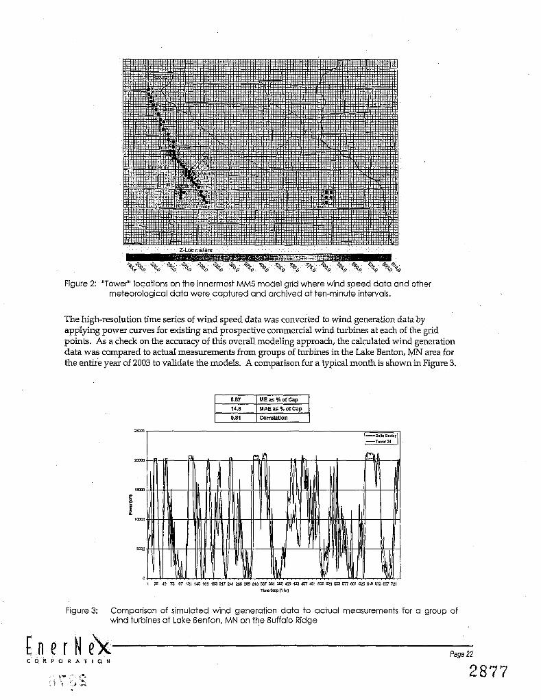
Figure 2: "Tower" locations on the innermost MM5 model grid where wind speed data and other meteorological data were captured and archived at ten-minute intervals.
The high-resolution time series of wind speed data was converted to wind generation data by applying power curves for existing and prospective commercial wind turbines at each of the grid points. As a check on the accuracy of this overall modeling approach, the calculated wind generation data was compared to actual measurements from groups of turbines in the Lake Benton, MN area for the entirk year of 2003 to validate the models. A comparison for a typical month is shown in Figure 3.
MAE as % of Cap
Correlation
n m asp (1 hr)
Figure 3: Comparison of simulated wind generation data to actual measurements for a group of wind turbines at Lake Benton, MN on the Buffalo Ridge
E n 4 r N t ; k C O R P O R A T I O N
Page 22
:r fl, t - 5 . , C .A ,.a
2877

The validation exercise showed that the numerical weather modeling approach produced high quality results. In months where the wind is driven by larger-scale weather patterns, the average error as a percentage of power production over the period was about 6%. In the summer months, where smaller-scale features such as thunderstorm complexes have more influence on wind speed, the mean error was larger, but still less than 9%. Mean absolute errors as a percent of capacity were approximately 15% or less for most months.
. A critical feature of the wind generation model for this study is that it captures the effects of the geographic dispersion of the wind generation facilities. For Xcel system operators, how the wind plants operate in the aggregate is of primary importance. This science-based modeling approach provides for representing the relationships between the behaviors of the individual plants over time more accurately than any other method.
Numerical weather simulations were also used in this task to develop a detailed characterization of the wind resource in Minnesota. Temporal and geographic variations in wind speed and power production over the southern half of Minnesota are characterized through a number of charts, graphs, and maps.
Task 1 concluded with a discussion of issues related to wind generation forecasting accuracy and a numerical experiment to compare various methods using the data and information compiled for developing the wind generation model. The accuracy of any weather-related forecast will decrease as the forecast horizon increases. Forecasts for the next few hours are likely to be sigruficantly more accurate than those for the next few days. The forecast experiment did show, however, that a more sophisticated method employing artificial intelligence techniques, a computational learning system (CLS) in conjunction with a numerical weather model, holds promise for significantly improving the accuracy of forecasts spanning a range from a few hours ahead through a two day period. This forecasting technique likely will have value for control area operators. Such techniques are in the development stages now, but will be commercially available in the coming years, and relevant to the study year for which this project is being conducted.
? Power Error Dlstrlbutlon
-1 - 0 8 - 0 8 - 0 7 -06 -05 -04 -03 - 0 2 -01 0 0 1 02 0 3 04 0 5 0 6 0 7 OE 0 9 1
Power error as fraction of r a s d
Figure 4: Frequency distribution of power error as a percent of rated capacity for 6,24 and 48 hour forecasts. Inset table shows the frequency of power errors less than 10,20 and 30 percent of rated capacity for the CLS 6;24 and 48 hour forecasts.

Since transmission constraints were not considered explicitly in this project, geographic variations in -
wind plant output are included in the analyses only to the extent that they affect the aggregated output profile of the total wind generation in the control area. However, the spatial variations could be combined with transmission constraints for a more refined evaluation, should that be desired in a future study.
Task 2:' Develop Xcel Energy System Model for 2010 Study Year - Ovelview and Results To conduct the technical analysis, models for both the wind generation development in Ivhnesota and the Xcel system in 2010 were developed. The wind generation scenario was derived from the numerical weather model data discussed in the previous section. In coordination with Xcel Energy and the Minnesota Department of Commerce, a county-by-county development scenario was constructed (Table 1) for the year 2010. The wind speed data created by the numerical weather model was converted to wind generation data at ten minute intervals for the three years of the simulation.
Table 1 : Minnesota Wind Generation Development Scenario - CY2010 ,
Xcel Energy predicts that the peak demand for their Minnesota control area will grow to 9933 MW in 2010. The projected resources to meet this demand are shown by type in Table 2 and graphically in Figure 5. Wind energy, which includes most of the wind generation assumed for this study, is assigned a capacity factor of 13.5% for purposes of this load and resources projection. Total capacity is projected to exceed peak demand by 15%.
Table 2: Xcel Capacity Resources for 201 0
E n e r N e k C O R P O R A T I O N page 2i 8 7 9

2001 AII.Source
Purchases 7 ,-Wnd Purchases
Q N W ~
1Cd-NSP Ownad
DOCS-NSP Owned
~ G c s - E x p h P h
.Om-Ohs
~ Q c s - I I S P SelWuMCTs
1OU-NSP Owmi
gHyh-NSPOwned
mWmMlOFNSP Owrd
mMH LolgTem Pvdena
OSIotTrn P* n o h s P ~ 1 B h s
12001 AWnnsPuztasen
1 I M r i P e
Gas Expansion plan-
Figure 5: Xcel supply resources for 2010 by type and fuel.
Since transmission issues were not to be explicitly considered in this study, the remaining component of the Xcel system "model" for the study year is the system load. To conduct the technical analyses as specified in the RFP, it was necessary to characterize and analytically q u a n w the system load in great detail. A variety of measurements of the existing load were collected. To represent the system load in 2010, measurements of the w e n t load (e.g. Figure 6) were scaled so that the peak hour for the year matched the expected peak in 2010 of 9933 MW.
1 - 900
Hours
Figure 6: Measurements of existing load data used for characterizing expected load in 201 0. Graph shows 72 hours of data collected at 4 second intervals by the Xcel Energy Management System [EMS)
E n e r N P k Page 25 C 0 !;P;Ot% A T I 0 N

The wind generation model derived from the numerical weather simulations was augmented with measurements from operating wind plants in Minnesota. The National Renewable Energy Laboratory (NREL) has been collecting very high resolution data from the Lake Benton I & I1 wind plants and the Buffalo Ridge substation in southwestern Minnesota for over three years. This data (Figure 7) was used to develop a representation of what the fastest fluctuations in wind energy delivery might look like to the Xcel system operators.
1.0
Total i
Total-Rate 0.8 h-
Delta i 3
Delta-Rate a 0.6
'Cd Echo i 5 & Echo Rate g -. -
2 0.4
Fox,Tot Rate 8 - - . - Golf i - 0.2
Golf-Rate , -
.o, 0 0 5 10 15 20 25
.o, i 25 - 60.60 Hour
Figure 7: NREL high-resolution measurement data from Lake Benton wind plants and Buffalo Ridge substation. Data show is power production sampled at one second intervals.
Task 3: Evaluation of Wind Generation Reliability Impacts - Overview and Results The purpose of the reliably analysis task of this study is to determine the ELCC (Effective Load Carrying Capability) of the proposed wind generation on the Xcel system. This problem was approached by modeling the system in the GE MARS (Multi-Area Reliability Simulation) program, simulating the system with and without the additional wind generation and noting the power delivery levels for the systems at a fixed reliability level. That reliability level is LOLE (Loss of Load Expectation) of 0.1 days per year.
The MARS program uses a sequential Monte Carlo simulation to calculate the reliability indices for a multi-area system by performing an hour by hour simulation. The program calculates generation and load for each hour of the study year, calculating reliability statistics as it goes. The year is simulated with different random forced outages on generation and transmission interfaces until the simulation converges.
In this study three areas are modeled, the Xcel system including all non-wind resources, an area representing Manitoba Hydro purchases and finally an area representing the Xcel Energy wind resources. The wind resources were separated to allow monitoring of hourly generation of the wind plant durFng the simulations.
The MARS model was developed based upon the 2010 Load and Resources table provided by Xcel Energy. In addition, load shape information was based upon 2001 actual hourly load data provided and then scaled to the 2010 adjusted peak load of 9933 MW.
The GE MARS input data file for the MAPP Reserve Capacity Obligation Review study was provided by MAPPCOR to assist in setting up the MARS data file for this study. State transition tables representing forced outage rate information and planned outage rate information for the Xcel

resources where extracted from the file where possible. In some cases it was difficult to map .
resources from the MAPP MARS file to the Load/Resources table provided by Xcel Energy. In those cases the resource was modeled using a generic forced outage rate for the appropriate type of generation (steam, combustion turbine, etc) obtained from the MAPP data file.
The model used multiple levels of wind output and probabilities, based on the multiple block capacities and outage rates that can be specified for thermal resources in MARS. In each Monte Carlo simulation, the MARS program randomly selects the transition states that are used for the simulation These states can change on and hour by hour basis, making MARS suitable for the modeling of the wind resources.
To find a suitable transition rate matrix, 3 years of wind generation data supplied by WindLogics was analyzed. That data was mapped on the proposed system and an hour by hour estimate of generation was calculated for the three yeirs. The generation was analyzed and state transitions were calculated to form the state transition matrix for input to MARS.
Figure 8: Results of reliability analysis for various wind generation modeling assumptions.
LOLE For XCEL Wind Study
This result shows that the ELCC of the system improves by 400 MW or 26.67% of nameplate with the addition of 1500 MW of wind resource. The existing 400 MW improved the ELCC by 135 MW or about 33.75%. This is an estimate as the nameplate of the existing wind resource was not known precisely.
-No W~nd (Base) -Lumped W~nd (1)
The results fall into the range of what would be "expected" by researchers and other familiar with modeling wind in utility reliability models. A remaining question, then, is one of the differences between the formal reliability calculation and the capacity accreditation procedure currently used in MAPP and being contemplated by other organizations.
-400 MW Existing (4)
-Wmd Modified Load
Geileratio~~ (MW) ELCC Without ELCC Wnh 400 MvV ELCCWnh 1500 MvV ELCCWnh 1500 hmnlVVInd as vVnd 9930 MW M n d 10065 MvV vVnd 10330 lvFN Load modifier - 10427 MvV

The W P procedure takes the narrowest view of the historical production data by limiting it to only those hours around the peak hour for the entire month, which potentially excludes some hours where the load is still substantial and there would be a higher risk of outage. Applying the W P procedure to the aggregate wind generation model developed for this study yields a minimum capacity factor of about 17%. It is still smaller, however, than the ELCC computed using lumped or seasonal wind models (26.7%).
Even though the formal reliability calculation using GE-MARS utilizes a very large number of "trials" (replications) in determining the ELCC for wind generation, the wind model in each of those trials is still based on probabilities and state transition matrices derived from just three years of data. Some part of the difference between the MAPP method and the formal reliability calculation, therefore, can be attributed to an insufficient data set for characterizing the wind generation. When the sample of historical data is augmented to the ten year historical record prescribed in the MAPP method, the capacity value determined by the MAPP method would Likely increase, reducing the magnitude of the difference between the two results.
This does not account for the entire difference between the methods, though. The MAPP procedure only considers the monthly peak hour, so the seasonal and diurnal wind generation variations as characterized in Task 1 of this project would lead to a discounting of its capacity value.
Table 3: Computed capacity values for 1500 MW wind generation scenario using MAPP accreditation procedure
January 394 26.3% February 498 33.2%
There are clear differences between the MAPP Capacity Credit method and the ELCC approach used in this study. The MAPP algorithm selects wind generation data from a 4-hour window that includes the peak, and is applied on a monthly basis. The ELCC approach is a risk-based method that q~~antifies the system risk of meeting peak load, and is primarily applied on an annual basis. ELCC effectively weights peak hours more than off-peak hours, so that two hypothetical wind plants with the same capacity factor during peak hours can receive different capacity ratings. In a case like this, the plant that delivers more output during high risk periods would receive a higher capacity rating than a plant that delivers less output during high risk periods.
The MAPP approach shares a fundamental weakness with the method adopted by PJM: the 4-hour window may miss load-hours that have sigruhcant risk, therefore ignoring an important potential contribution from an intermittent generator. Conversely, an intermittent generator may receive a

, capacity value that is unjustifiably high because its generation in a high-risk hour is lower than during the 4-hour window.
Because ELCC is a relatively complex, data-intensive calculation, simplified methods could be developed at several alternative levels of detail. Any of these approaches would fully capture the system's high-risk hours, improving the algorithm beyond what would be capable with the fixed, narrow window in the current MAPP method. Any of the methods can also be applied to several years of data, which could be made consistent with current MAPP practice of using up to 10 years of data, if available.
Task 4: Evaluation of Wind Generation Integration Costs on the Operating lime Frame - Ovenriew and Results At significant levels relative to loads and other generating resources in the control area, wind generation has the potential to increase the burden of managing the power system, thereby increasing overall costs. The economic consequences of this increased burden are term "integration costs", and are the ultimate focus of this research effort. Integration costs for wind generation stem from two primary factors:
Wind generation exhibits sigzuficant and mostly uncontrollable variability on all of the time scales relevant to power system operations - seconds, minutes, hours, days;
The ability to pre'dict or forecast wind generation for forward time periods is lower than that for conventional resources, and declines as the forecast horizon moves outward.
How the combination of these characteristics can impact the overall cost of operating the system can be thought of in the following way: For a given control area, the uncertainties associated with scheduling and operating generating resources, namely errors in load forecasts or unexpected outages or operating limitations of certain generating units - are well known based on history and experience. Procedures have evolved to accommodate these uncertainties, such that for a particular load magnitude or pattern, the supply resources are deployed and operated in a manner that minimizes the total production cost. The additional variability that comes with a sigruficant amount of wind generation in the control area requires that the existing supply resources be used in a different manner. Increased uncertainty related to the probable errors in wind generation forecasts for future periods can lead to either more conservatism in the deployment of generating resources (and more cost) or operating problems that arise due to the differences between the forecast and actual wind generation in a particular hour (again, with possibly added cost).
The "value" of wind generation is separate from the integration costs. The objective here is to determine how the cost to serve load that is not served by wind generation 2 affected by the plans and procedures necessary to accommodate the wind generation and maintain the reliability and security of the power system.
In this project, the integration costs are differentiated by the time scale over which they might be incurred, with the total integration cost being the sum of the individual components. The time frames and operating functions of interest include:
Regulation, which occurs on a very short time scale and involves the automatic control of a sufficient amount of generating capacity to support frequency and maintain scheduled transactions with other control areas;
Unit commitment and scheduling, which are operations planning activities aimed at developing the lowest cost plan for meeting the forecast control area demand for the next day or days;

Load following and other intra-hourly operations that involve the deployment of generating resources to track the demand pattern over the course of the day, and adjustments to compensate for changes in the control area demand as the load transitions through the hours and periods of the daily load pattern.
A variety of analytical techniques were employed to quantify the impacts of 1500 MW of wind generation on the Xcel control area. The following sections describe the methods used in each of the three time frames along with the results and conclusions.
Regulation
The aggregate load in the control area is constantly changing. The fastest of these changes can be thought of as temporary ups and downs about some longer term pattern. Compensating in some way for these fast fluctuations is necessary to meet control area performance standards and contribute to the frequency support for the entire interconnection. Regulation is that generating capacity that is deployed to compensate for these fast changes.
The regulation requirement for the Xcel system load in 2010 was projected by analyzing high- resolution measurements of the current load. By applying appropriate smoothing techniques, the fluctuating component responsible for the regulating burden can be isolated. Figure 9 shows the result of this algorithm for one hour of the Xcel load. The blue line is actual instantaneous load, sampled once every four seconds; the red line is the computed trend through the hour. The difference between the actual load and the trend is the regulating characteristic.
9 2
HOUR - Load Trend - Inst. Load
Figure 9: Actual load (blue) and hourly trend (red) for one hour.
Wind generation also exhibits fluctuations on this time scale, and thereby may increase the requirement for regulating capacity. The regulation trends are nearly energy neutral (the incremental energy for the time spent above the trend is equal to that spent below the trend), so the economic impact is the opportunity cost related to reserving the necessary amount of generation capacity to perform this function.
Data from NREL monitoring at the Lake Benton wind plants and the Buffalo Ridge substation was used to estimate the regulation requirements for the 1500 MW of wind generation in this study. Figure 10 contains a short sample of this data, which is collected at one second intervals. The graph shows actual wind generation@ percent of rated capacity) over a 24-hour period for several different collections of wind turbines, each of which is connected to the Buffalo Ridge substation.
E n t r N ~ k Page 30 C O R P O R A T I O N
* rr d*.

0 10 15 25 Hour
- Total ----- Delta - - Echo Foxtrot
- Golf
Figure 10: Typical daily wind generation for Buffalo Ridge plants data sampled at one second intervals for 24 hours.
The sigruficant item to note from the figure is that the red trace corresponds to a measurement of 280 individual turbines. The other traces area from subsets of this overall number. Analysis of the data clearly shows that the fast fluctuations, when expressed as a percentage of the rated capacity of the turbines comprising the group, declines substantially as the number of turbines increases.
Because of the factors responsible for these fast fluctuations, it can be reasonably concluded that variations from one group of turbines are not dependent on or related to those from a geographically separated group. In statistical terms, the variations are uncorrelated.
It is further assumed that the fast fluctuations from a group or groups of wind turbines are not related to the fast fluctuations in the system load, since there is no plausible explanation for why they would be related. Of interest here is how the fluctuations of the system load with wind generation added compare to those from the system load alone.
For uncorrelated variations, statistics provides a straight-forward way to estimate the characteristics of the system load and wind combination. For normally-distributed random variables, the standard deviation of the combination can be computed from the standard deviations of the individual variables with the following formula:
The standard deviation of the combination of the variables is the square root of the sum of the squares of the individual standard deviations.
This statistical property can be applied to the random variables representing the fast fluctuations in wind generation and the load. In the study scenario, it was assumed that the 1500 MW of wind generation was actually comprised of 50 individual 30 MW wind plants. The re,p.lation requirement for each of these plants was estimated to be 5% of the nameplate rating, based on the analysis of the measurement data from Buffalo Ridge. The standard deviation of the load fluctuations alone was calculated to be 20.2 MW for 2010. Applying the formula from above, the standard deviation of the Xcel system load in 2010 plus 1500 MW of wind generation is 22.8 MW.
A translation to regulating requirements can be made by recognizing that for the random, normally- distributed variables, over 99% of all of the variations will fall within plus or minus three standard
E n ~ r N e k /
Page 31 c o R P p ~ l n i I o N
\ : ,_s . .
2886

deviations. So multiplying the results above by three leads to the conclusion that the addition of wind would increase the regulation requirement by (22.8 - 20.2) x 3 = 7.8 MW.
The "cost" of this incremental regulating requirement can be estimated by calculating the opportunity cost (revenue less production cost for energy that cannot be sold from the regulating .
capacity) for 7.8 MW of generating capacity. Xcel currently employs large fossil units for regulation, so the production cost is relatively low, around $10/MWH. If it is assumed that this energy could be sold at $25/MWH, the opportunity cost over the entire year would be just over $1,000,000.
Dividing the total cost by the expected annual energy production of the 1500 MW of wind generation (using an average capacity factor of 35%) yields an incremental regulation cost of $0.23/MWH.
Capacity value provides an alternative method for costing the incremental regulation requirement. Using a value of $10/kW-month or $120/kw-year, the annual cost of allocating an additional 7.8 MW of capacity to regulation duty comes out to be $936,000, about the same as the number arrived at through the simple opportunity cost calculation. This number and the previous result are not additive, however. By either method, the cost to Xcel for providing the incremental regulation capacity due to the 1500 MW of wind generation in the control area is about $1 million per year.
Unit Commitment and Scheduling - Hourly Impacts Because many generating units cannot be stopped and started at will, forward-looking operating plans must be developed to look at the' expected demand over the coming days and commit generation to meet this demand. This plan should result in the lowest projected production cost, but must also acknowledge the limitations and operating restrictions of the generating resources, provide for the appropriate amount of reserve capacity, and consider firm and opportunity sales and purchases of energy.
The approach for quantifying the costs that could be incurred with a significant amount of wind generation was based on mimicking the activities of the system schedulers, then calculating the costs of the resulting plans. The input data for the analysis consisted of hourly load data, wind generation data, and wind generation forecast data for a two year period. Figure 11 contains a block diagram of the process. For each day of the two year data set, a reference case was developed that assumed that the daily energy from wind generation was known precisely, and that it was delivered in equal amounts over the 24 hours of the day. This reference case was selected since it represents wind as a resource that would have the mini~~~um impact on the operation of other supply resources.
Unii ~ o ~ m l b n a n l Houdy Wind Develop OA 6 Schndulu Gensrabn Hourly Wlnd Bused an Forecartr
Gen. Forecasl
una Cornmibnent 6 Scheduling
(Opllml2allon)
Hourly SysLem Loud Dsls
Cmab 'FlaB Prnm for Daily Whd Eneqy
Figure 1 1 : Block diagram of methodology used for hourly analysis.
4 (Opllrnl~lfon] C a i ~ I e I e Auua
Daly E n q Delbemd
b
+
Page 32 C O R P O R A T I O N
2887
Unl Commlbned a scheduong
Hourly "Slrnulatfon" wlth conomkdirpakh
O(avellaMeUni19

The next set of cases represented the actions of the system schedulers. The projected load and an hour-by-hour wind generation forecast were input to the unit commitment and scheduling program. The program then determined the lowest cost way to meet the load and accommodate the wind generation as it was forecast to be delivered. The forecast wind generation was then replaced by "actual" wind generation. Then, a simulation of the same day was conducted. However, instead of allowing the program to change the planned deployment of generating resources, only the resources available per the plan developed with the wind generation forecast data could be used to meet the actual load, minus, of course, that load served by wind generation on an hourly basis.
This method was applied to 730 individual days that represented actual loads from 2002 and 2003 (scaled so that the peak matches that for 2010). Wind generation data from the numerical simulation model for each of the days over those two years represented "actual" wind generation. Using results from the forecasting experiment of Task 1, an additional time series was created to represent wind generation forecast data for those years (a comparison of forecast vs. actual as used in this study is shown in Figure 12). This set contained errors that are consistent with what would be expected from a wind generation forecast developed on the morning of the previous day (a time horizon of 16 to 40 hours).
Table 4 shows the results by month for the hourly analysis. The average hourly integration cost based on simulation of the commitment and scheduling process for 24 months is calculated to be $4.37/MWH of wind energy. The assumptions used in the hourly analysis make that cost a relatively conservative estimate - they are on the higher end of the range of results that could be generated by -
varying the assumptions. There appear to be a number of opportunities and mechanisms that would reduce those costs. The more important of these are related to the emergence of liquid wholesale markets administered by MIS0 which would provide an alternative to using internal resources to compensate for the variability of wind generation Another is the analysis and development of algorithms for unit commitment and scheduling that explicitly account for the uncertainty in wind generation forecasts and lead to operating strategies that "win1' more than they "lose" over the longer term. Closely related to such algorithms are further developments of wind generation forecasting techniques and analyses that would provide the appropriate input data.
" 63 62 64 66 68 70 72 74
- Day Actual - - - - - Forecast
Figure 12: Wind generation forecast vs. actual for a two week period.
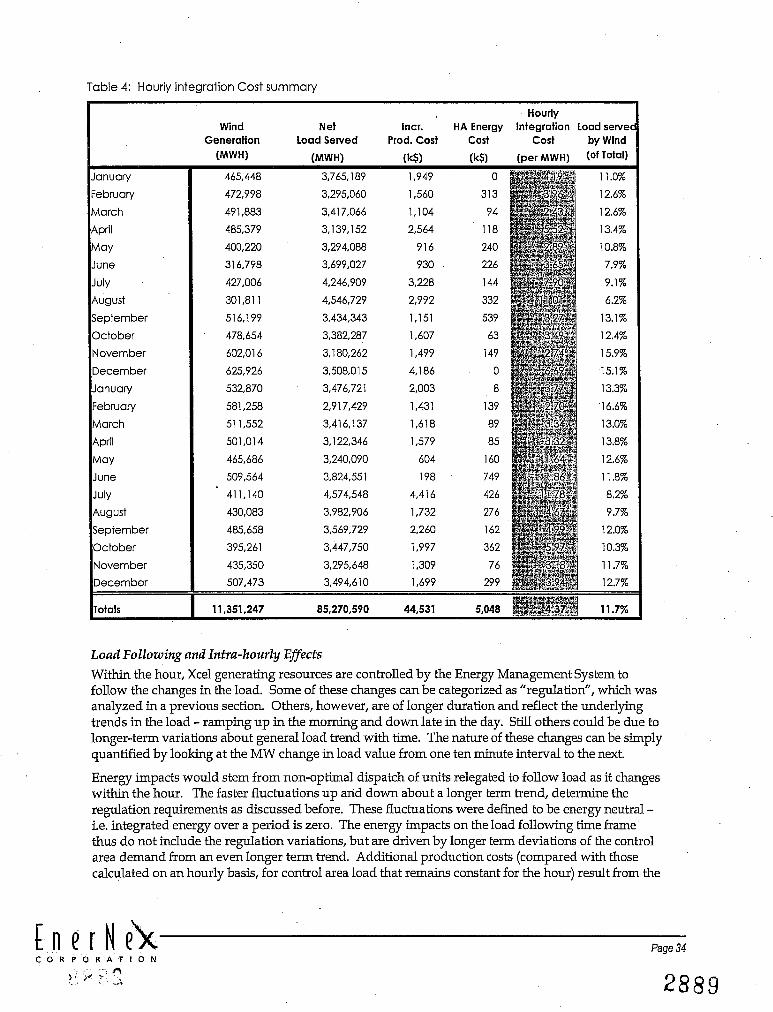
Table 4: Hourly Integration Cost summary
Load Following and Intm-hourly Eflects Within the hour, Xcel generating resources are controlled by the Energy Management System to follow the changes in the load. Some of these changes can be categorized as "regulation", which was analyzed in a previous section. Others, however, are of longer duration and reflect the underlying trends in the load - ramping up in the morning and down late in the day. Still others could be due to longer-term variations about general load trend with time. The nature of these changes can be simply quantified by looking at the MW change in load value from one ten minute interval to the next.
Energy impacts would stem from non-op,hal dispatch of units relegated to follow load as it changes within the hour. The faster fluctuations up and down about a longer term trend, determine the regulation requirements as discussed before. These fluctuations were defined to be energy neutral - i.e. integrated energy over a period is zero. The energy impacts on the load following time frame thus do not include the regulation variations, but are driven by longer term deviations of the control area demand from an even longer term trend. Additional production costs (compared with those calculated on an hourly basis, for control area load that remains constant for the hour) result from the
E n ~ r N e ' k Page 34 C O R P O R A T l O N

load following units dispatched to different and possibly non-optimal operating levels to track the load variation through the hour.
The additional costs of this type attributable to wind generation are related, then, to how it alters the intra-hourly characteristic of the net control area demand. High-resolution load data provided by Xcel Energy and scaled to the year 2010 along with wind generation data from the numerical simulation model were analyzed to elicit the characteristics of this behavior at ten-minute intervals.
Figure 13 shows a weekly trend of the changes from one ten-minute interval to the next for the system load and wind generation. It is apparent from the plot that the load exhibits sigruficantly more variability than does wind generation.
SOD
4W 300 230
1W b I 0
-1 W -230
-307 -4W
-5M) 55CO 5524 5548 5572 5596 5620 5644 5668
Hour - 10 rnin. C h a n g e in Load - 10 rnin. C h o n g e in Wind Generation
Figure 13: Weekly time series of ten-minute variations in load and wind generation.
An entire year of data - almost 50,000 ten-minute data points - was analyzed to develop a statistical distribution of these changes (Figure 14). The results show that wiTld generation has only a minor influence on the changes from one interval to the next, and most of the effect is to increase the relatively small number of larger-magnitude changes.
-1 003 -500 0 533 1030 1 10 rnin. Change in (Load - Wind)
10 min. Change in Load
Figure 14: Control area net load changes on ten minute intervals with and without wind generation.

The same data was also analyzed to examine the variation from a longer term trend that tracks the hour-by-hour daily load pattern. The distributions of these variations with and without wind generation over the year of data are shown in Figure 15.
tv\w Load -Wind Generation
1 Load Only
Figure 15: Variation at ten-minute increments from daily "trend" pattern, with and without wind generation.
The numerical results are similar to those described previously that considered the absolute changes on ten-minute increments. The standard deviation of the distribution of deviations from the hourly trend for the load only is 53.4 MW; with wind generation in the control area, the standard deviation increases to 64 MW.
In the earlier study, results from simulations of a limited number of "typical" hours along with several simphfymg assumptions were extrapolated to annual projections. A cost impact of $0.41/MWH was assigned to wind generation due the variability at a time resolution of five minutes. However, one of the major simplifications was that only the wind generation exhibited significant variability from a smooth hourly trend, so that all costs from the intra-hourly simulations beyond those calculated at the hourly level could be attributed to wind generation.
The data analyses here lead to a different conclusion The system load does vary sigruhcantly about a smoother hourly trend curve, and may also vary substantially from one ten-minute interval to the next. With this as the backdrop, it was shown that the addition of wind generation to the control area would have only slight impacts on the intra-hour variability of the net control area demand. It also appears that the corresponding changes in wind generation and those in the system load are uncorrelated, which substantially reduces the overall effect of the variations in wind generation within the hour.
In quantitative terms, for the system load alone, just over 90% of the ten-minute variations from the hourly trend value are less than 160 MW. With wind generation, that percentage drops to 86%, or stated another way, 90% of the ten-minute variations from the hourly trend value are less than 180 MW.
The original project plan called for simulations to be used for quantifying the energy cost impacts at the sub-hourly level. This was the approach taken in the earlier study of the Xcel system, and thought to be the most direct method for this assessment. In light of the results of the intra-hourly data analysis, it was determined detailed chronological simulations would be of very limited value for determining any incremental cost impacts for intra-hourly load following. With a very slight effect on the characteristics of the intra-hourly control area demand characteristic as evidenced by the
E n e r N e k Page 36 C O R P O R , , A T I O N
, t , <; ' ' " L# -,* 2891

approximately 10 MW change in the standard deviations, calculated effects on production cost would likely be in the "noise" of any deterministic simulations.
Based on the analysis here, it is concluded that the $0.41/MWH of wind generation arrived at in the previous study was artificially high since the load was assumed to vary smoothly during the hour. Also, the statistical results presented here support the conclusion that the increase in production cost on an intra-hourly basis due to the wind generation considered here would be negligible.
The results do show, however, that wind generation may have some influence on control performance as the number of large deviations from one interval to the next or from the longer-term trend of the net control area demand is sigruficantly increased. An expansion of the distributions of ten-minute changes with and without wind generation is shown in Figure 16. Wind generation substantially increases the number of larger-magnitude excursions over the course of the year.
" -503 -4M) -330 -233 -lW 0 133 XX) 330 403 500 1 10 min. Change in (Load -Wind) n 10 rnin. Change in Load
Figure 16: Expanded view of Figure 14.
The total number of these large excursions is not sigruficant from an energy standpoint, since the number is a small fraction of the total number over the year. There are implications, however, for control performance of the Xcel system. To assess this potential impact, increases in the occurrences of control area demand change of a given magnitude were "counted". Table 5 shows the number of occurrences over the sample year of data where the net control area load (load minus wind generation) changed more than a given amount (up or down) in one ten minute period.
E n P I N tk Page 37 C O , R $ ~ ~ ' $ A T I 0 N

Table 5: Ten-minute Variations in Control Area Demand, with and without Wind Generation
With a ramping capability of 140 MW per ten minute period, control performance (CPS2, in NERC .terminology) would be comfortably above the minimum requirement with or without wind generation. Or, from another perspective, if the current CPS2 performance is 94%, maintaining that performance level with the addition of 1500 MW of wind generation would require somewhere between 1 and 2 MW/minute of additional load following capability.
,
Conclusions The analysis conducted in this task indicates that the cost of integrating 1500 MW of wind
generation into the Xcel control area in 2010 are no higher than $4.60/MWH of wind generation, and are dominated by costs incurred by Xcel to accommodate the sigruficant variability of wind generation and the wind generation forecast errors for the day-ahead time frame.
The total costs include about $0.23- as the opportunity cost associated with an 8 hlW increase in the regulation requirement, and $4.37- of wind generation attributable to unit commitment and scheduling costs. The increase in production cost due to load following within the hour was determined by a statistical analysis of the data to be negligible. The intra-hour analysis also showed that an incremental increase in fast ramping capability of 1-2 MW/minute would be necessary to maintain control performance at present levels. This specific impact was not monetized.
The analytical approach for assessing costs at the hourly level in this study compares the actual delivery of wind energy to a reference case where the same daily quantity of wind energy is delivered as a flat block. In addition to costs associated with variability and uncertainty, the total integration cost then will contain a component related to the differential time value of the energy delivered. If more wind energy is actually delivered "off-peak" relative to the reference case, when marginal costs are lower, this differential value will show up in the integration cost. The total integration cost calculated by this method is still a meaningful and useful value, but care must be taken not to ascribe all of the integration cost to uncertainty and variability of wind generation output.
Wind generation also results in a much larger ramping requirement from hour to hour. The costs associated with this impact are captured by the hourly analysis, as the unit commitment and schedule must accommodate any large and sudden changes in net control area demand in either the forecast optimization case, or in the simulation with actual wind generation. In the optimization case that utilizes wind generation forecast data, generating resources must be committed and deployed to follow control area demand while avoiding ramp rate violations. In the simulation cases with actual wind generation, changes due to wind generation that cannot be accommodated result in "unserved energy" in the parlance of the unit commitment software, which really means that it must be met through same-day or more probably next-hour purchases.
Page 38 C O R P O R A T I O N 2893

Some specific conclusions and observations include:
1. While the penetration of wind generation in this study is low with respect to the projected system peak load, there are many hours over the course of the year where wind generation is actually serving 20 to 30% (or more) of the system load. A combination of good plans, the right resource mix, and attractive options for dealing with errors in wind generation forecasts are important for substantially reducing cost impacts.
2. That said, the cost impacts calculated here are likely to be somewhat overstated since little in the way of new strategies or changes to practices for short-term planning and scheduling were included in the assumptions, and since the hour-ahead adjustments in the study are made at a price closer to the marginal cost of internal resources than those in a liquid wholesale energy market.
3. The incremental regulation requirement and associated cost for accommodating 1500 MW of .
wind generation, while calculable, is quite modest. The projected effect of geographic diversity together with the random and uncorrelated nature of the wind generation fluctuations in the regulating time frame, as shown by the statistical analysis, have a dramatic impact on this aspect of wind generation.
4. Large penetrations of wind generation can impact the hourly ramping requirements in almost all hours of the day. On the hourly level, this results in deployment of more resources to follow the forecast and actual ramps in the net system load, thereby increasing production costs.
5. Wind generation integration costs are sensitive to the deployment of units, which is also a function of the forecast system load. The results seem to indicate that these costs can be high over a period when expensive resources'are required to compensate for the hourly variability, even when the total wind generation for the period might be low.
6. For the study year of 2010, the cost of integrating 1500 MW of wind generation into the Xcel- NSP control area could be as high as $4.60/MWH of wind energy where the hour-by-hour forecast of wind for 16 to 40 hours ahead has a mean absolute error of 15% or less. The total integration cost is dominated by the integration cost at the hourly level, and assumes no sigruficant changes to present strategies and 'practices for short-term unit commitment and scheduling.
7. The MIS0 market cases demonstrate that the introduction of flexible market transactions to assist with balancing wind generation in both the day-ahead scheduling process and the day one hour ahead has a dramatic positive impact on the integration costs at the hourly level. For example, in August the hourly cost was reduced by two thirds.
Results of the hourly analysis are considered to be quite conservative - they are on the high end of the range of results that could be generated by varying the assumptions. While the methodology is relatively robust and thought by the researchers to be straightforward and consistent with industry practice, a number of assumptions were made to faditate analysis of a large set of sample days - two years of days unique in peak load, load pattern, actual and forecast wind generation. The input data for the hourly analysis was developed in such a way that any correlations between Xcel control area load and the wind resource in the upper Midwest are actually embedded in the datasets.
Much of the conservatism in the hourly analysis stems from the simplification of many decisions that would be made by knowledgeable schedulers, traders, and system operators to reduce system costs and/or increase profits. This leads to the use of resources which are under the control of the unit commitment program to accommodate the variability of wind generation and the day-ahead wind generation forecast errors. In months with higher electric demand, these resources can be relatively expensive.

Energy purchases and sales are a potential alternative to internal resources. In the hourly analysis, these transactions were fixed, not allowing for the day-ahead flexibility that might currently exist for judicious use of inexpensive energy to offset the changes in wind generation. Optimizing these transactions day by day would have prevented evaluation of the statistically sigruficant data set of load and wind generation, and would have been to difficult to define objectively.
Given the likely sources of the integration cost at the hourly level, it is apparent that a better strategy for purchase and sale transactions scheduled even day-ahead would reduce integration costs at the hourly level. This leads naturally to considering how wholesale energy markets would affect wind integration costs.
The planning studies conducted by MIS0 show that wholesale energy is relatively inexpensive in the upper Midwestern portion of their footprint. Transmission constraints do come into play on a daily and seasonal basis, but interchange limits for most of Minnesota are reasonably high relative to the amount of wind generation considered in this study. The ability to use the wholesale energy market as a balancing resource for wind generation on the hourly level has sigruficant potential for reducing the integration costs identified here.
Wholesale energy markets potentially have advantages over bi-lateral transactions as considered simplistically in this study. In day-ahead planning, for example, it would be possible to schedule variable hourly transactions consistent with the forecast variability of the wind generation. Currently, day-ahead bi-lateral transactions are practically limited to profiles that are either flat or shapeable to only a limited extent. Hour-ahead purchases and sales at market prices would provide increased flexibility for dealing with sigruficant wind generation forecast errors, displacing the more expensive units or energy fire sales that sometimes result when relying on internal resources.
Page 40 C O R P O R A T I O N 2895

Integration Group
Utility Wind Integration State of the Art
Prepared by
Utility Wind Integration Group in cooperation with
American Public Power Association (APPA) Edison Electric Institute (EEI)
National Rural Electric Cooperative Association W C A )
Utility Wind Integration Group P.O. Box 2787 Reston, VA 20195
703-860-5160 www.nwig.org
May 2006
Joint Intervenors Exhibit 4 -- B

Overview and Summary
In just five years from 2000-2005, wind energy has become a significant resource on many electric utility systems, with over 50,000 MW of nameplate capacity installed worldwide at the end of 2005. Wind energy is now "utility scale" and can affect utility system planning and operations for both generation and transmission. The utility industry in general, and transmission system operators in particular, are beginning to take note. At the end of 2005, the Power Engineering Society (PES) of the Institute of Electrical and Electronic Engineers (IEEE) published a special issue of its Power & Energy Magazine (Volume 3 , Number 6, NovemberiDecember 2005) focused on integrating wind into the power system. This document provides a brief summary of many of the salient points from that special issue about the current state of knowledge regarding utility wind integration issues. It does not support or recommend any particular course of action or advocate any particular policy or position on the part of the cooperating organizations.
The discussion below focuses on wind's impacts on the operating costs of the non-wind portion of the power system and on wind's impacts on the electrical integrity of the system. These impacts should be viewed in the context of wind's total impact on reliable system operation and electricity costs to consumers. The case studies summarized in the magazine address early concerns about the impact of wind power's variability and uncertainty on power system reliability and costs. Wind resources have impacts that can be managed through proper plant interconnection, integration, transmission planning, and system and market operations.
On the cost side, at wind penetrations of up to 20% of system peak demand, system operating cost increases arising from wind variability and uncertainty amounted to about 10% or less of the wholesale value of the wind energy.' These incremental costs, which can be assigned to wind-power generators, are substantially less than imbalance penalties generally imposed through Open Access Transmission Tariffs under FERC Order No. 888. A variety of means - such as commercially available wind forecasting and others discussed below - can be employed to reduce these costs. In many cases, customer payments for electricity can be decreased when wind is added to the system, because the operating-cost increases could be offset by savings from displacing fossil fuel generation.
Further, there is evidence that with new equipment designs and proper plant engineering, system stability in response to a major plant or line outage can actually be improved by the addition of wind generation. Since wind is primarily an energy - not a capacity - source, no additional generation needs to be added to provide back-up capability provided that wind capacity is properly discounted in the determination of generation
These conclusions will need to be reexamined as results of higher-wind-penetration studies -- in the range of 25% to 30% of peak balancing-area load -- become available. However, achieving such penetrations is likely to require one or two decades. During that time, other significant changes are likely to occur in both the makeup and the operating strategies of the nation's power systems. Depending on the evolution of public policies, technological capabilities, and utility strategic plans, these changes can be either more or
- . less accommodating to the natural characteristics of wind power plants. * c

capacity adequacy. However, wind generation penetration may affect the mix and dispatch of other generation on the system over time, since non-wind generation is needed to maintain system reliability when winds are low.
Wind generation will also provide some additional load carrying capability to meet forecasted increases in system demand. This contribution is likely to be up to 40% of a typical project's nameplate rating, depending on local wind characteristics and coincidence with the system load profile. Wind generation may require system operators to carry additional operating reserves. Given the existing uncertainties in load forecasts, the studies indicate that the requirement for additional reserves will likely be modest for broadly distributed wind plants. The actual impact of adding wind generation in different balancing areas can vary depending on local factors. For instance, dealing with large wind output variations and steep ramps over a short period of time could be challenging for smaller balancing areas, depending on the specific situation.
The remainder of this document is divided into four sections: wind plant interconnection, wind plant integration, transmission planning and market operation, and accommodating more wind in the future.
Wind Plant Interconnection
Wind power plant terminal behavior is different from that of conventional power plants, but can be compatible with existing power systems. With current technology, wind-power plants can be designed to meet industry expectations such as riding through a three-phase fault, supplying reactive power to the system, controlling terminal voltage, and participating in SCADA system operation. Increased demands will be placed on wind plant performance in the future. Recent requirements include low voltage ride-through capability, reactive power control, voltage control, output control, and ramp rate control. Future requirements are likely to include post-fault machine response characteristics more similar to those of conventional generators (e.g., inertial response and governor response). Better dynamic models of wind turbines and aggregate models of wind plants are needed to perform more accurate studies of transmission planning and system operation. In areas with limited penetration, modem wind plants can be added without degrading system performance. System stability studies have shown that modern wind plants equipped with power electronic controls and dynamic voltage support capability can improve system performance by damping power swings and supporting post-fault voltage recovery. Because of spatial variations of wind from turbine to turbine in a wind plant - and to a greater degree from plant to plant - a sudden loss of all wind power on a system simultaneously due to a loss of wind is not a credible event.
Wind Plant Integration
Utility planners traditionally view new generation primarily in terms of its capacity to serve peak demand. But wind is primarily an energy resource. Its

primary value lies in its ability to displace energy produced from the combustion of fossil fuels and to serve as a hedge against fuel price risk and future restrictions on emissions. The addition of a wind plant to a power system does not require the addition of any backup conventional generation since wind is used primarily as an energy resource. In this case, when the wind is not blowing, the system must rely on existing dispatchable generation to meet the system demand. Wind plants provide additional planning reserves to a system, but only to the extent of their capacity value. Capacity for day-to-day reliability purposes must be provided through existing marlcet mechanisms and utility unit commitment processes. The capacity value of wind generation is typically up to 40% of nameplate rating, and depends heavily on the correlation between the system load profile and the wind plant output. -
-
The addition of a wind plant to a power system increases the amount of v and uncertainty of the net load. This may introduce measurable changes in the amount of operating reserves required for regulation, ramping and load-following. Operating reserves may consist of both spinning and non-spinning reserves. In two major recent studies, the addition of 1,500 MW and 3,300 MW of wind (15% and lo%, respectively, of system peak load) increased regulation requirements by 8 MW and 36 MW, respectively, to maintain the same level of NERC control performance standards. Fluctuations in the net load (load minus wind) caused by greater variability and uncertainty introduced by wind plants have been shown to increase system operating costs by up to about $5/MWH at wind penetration levels up to 20%. The greatest part of this cost is associated with the uncertainty introduced into day-ahead unit commitment due to the uncertainty in day-ahead forecasts of real- time wind energy production. The impact of adding wind generation can vary depending on the nature of the dispatchable generating resources available, market and regulatory environment, and characteristics of the wind generation resources as compared to the load. Dealing with large output variations and steep ramps over a short period of time (e.g., within the hour) could be challenging for smaller balancing areas, depending on their specific situation. Wind's variability cannot be treated in isolation from the load variability inherent in the system. Because wind and load variability are statistically uncorrelated, the net increase of variability due to the addition of wind is less than the variability of the wind generation alone. Commercially available wind forecasting capability can reduce the costs associated with day-ahead uncertainty substantially. In one major study, state-of- the-art forecasting was shown to provide 80% of the benefits that would result from perfect forecasting. Implementation of wind-plant-output forecasting in both power market operation and system operations planning in the control room environment is a critical next step in accommodating increasing amounts of wind penetration in power systems.

Transmission Planning and Market Operation
Upgrades or additions to transmission facilities may be needed to access locations with large wind-energy potential. Current transmission planning processes are able to identify solutions to transmission problems, but the time required for implementation of solutions often exceeds wind-plant permitting and construction times by several years. Well-functioning hour-ahead and day-ahead markets provide the best means of addressing the variability in wind plant outp~~t. Energy imbalance charges based on actual costs or market prices provide appropriate incentives for accurate wind forecasting. Since wind plant operators have no control over the wind, penalty charges applied to wind imbalances do not improve system reliability. Market products and tariff instruments should properly allocate actual costs of generation energy imbalance. Wind turbine output or ramp rates may need to be curtailed for limited periods of time to meet system reliability requirements economically. Consolidation of balancing areas or the use of dynamic scheduling can improve system reliability and reduce the cost of integrating additional wind generation into electric system operation.
Accommodating More Wind in the Future
Understanding and quantifying the impacts of wind plants on utility systems is a critical first step in identifying and solving problems. A number of steps can be taken to improve the ability to integrate increasing amounts of wind capacity on power systems. These include:
o Improvements in wind-turbine and wind-plant models o Improvements in wind-plant operating characteristics o Carefully evaluating wind-integration operating impacts o Incorporating wind-plant forecasting into utility control-room operations o Making better use of physically (in contrast with contractually) available
transmission capacity o Upgrading and expanding transmission systems o Developing well-functioning hour-ahead and day-ahead markets, and
expanding access to those markets o Adopting market rules and tariff provisions that are more appropriate to
weather-driven resources o Consolidating balancing areas into larger entities or accessing a larger
resource base through the use of dynamic scheduling.
The Power & Energy Magazine articles summarized in this document are available to IEEE PES members at the following link: 11~://www.ieee.or~/portal/site/pes/1nenuite1n.bfd2bcf5a5608058fb2275875bac26c8/inde x.isp?&pName=pes home
and to UWIG members at www.uwig.org through the Members link.


Grid Impacts of Wind Power Variability: Recent Assessments from a Variety of Utilities in the United states'
Brian Parsons and Michael ~ i l l i ~ a n " , Consultant National Renewable Energy Laboratory
J Charles Smith Utility Wind Integration Group
Edgar DeMeo Renewable Energy Consulting Services, Inc.
Brett Oakleaf Xcel Energy
Kenneth Wolf Minnesota Public Utilities Commission
Matt Schuerger Energy Systems Consulting Services, LLC
Robert Zavadil EnerNex Corporation
Mark Ahlstrom WindLogics
Dora Yen Nakafuji California Energy Commission
Introduction and Background
During 2005 apprbxirnately 2,500 MW of yind capacity was added in the United States, which brought installed wind capacity to about 9,150 MW. Although the total wind capacity in the United States is less than in some countries, wind energy has caught the attention of some utilities that depend on natural gas to generate power. There is evidence that wind development will continue at significant levels in the United States for the next several years, although it may be sensitive, to a number of factors that include transmission availability, wind turbine availability, prices of wind technology and competing fuels, production tax credit availability, and states' renewable portfolio standards (RPSs).
This trend has helped induce electricity providers to investigate the potential impact of wind on the power system. Because of wind power's unique characteristics, many concerns are based on the increased variability that wind contributes to the grid, and most U.S. studies have focused on this aspect of wind generation. Grid operators are also concerned about the ability to predict wind generation over several time scales.
In this report we discuss some recent studies that have occurred in the United States since our previous work [2,3]. The key objectives of these studies were to quantifi the physical impacts and costs of wind generation on grid operations and the associated costs. Examples of these costs are (a) committing unneeded generation, (b) allocating more load- following capability to account for wind variability, and (c) allocating more regulation capacity. These are referred to as "ancillary service" costs, and are based on the physical system and operating characteristics and procedures. This topic is covered in more detail by Zavadil et al. [4].
Time ~ r a m e s of Wind's Impact
W i d can have an impact on several time scales that correspond to grid operations. The shortest is generally in the range of milliseconds to seconds, and is the domain of system dynamic stability studies. Most wind integration studies
* Portions of this paper have been adapted from IEEE Power & Energy, NovemberlDecember 2005 [I]. I.
Employees of the Midwest Research Institute under Contract No. DE-AC36-99G010337 with the U.S. Dept. of Energy have authored this work. The United States Government retains, and the publisher, by accepting the article for publication, acknowledges that the United States Government retains a non-exclusive, paid-up, irrevocable, worldwide license to publish or reproduce the published form of this work, or allow others to do so, for the United States Government purposes.
2901 Joint Intervenors Exhibit 4 -- C

focus on longer time scales, but the stability time frame is a concern and recent developments in the United States have addressed this issue. The most important is the Federal Energy Regulatory Commission (FERC) limited grid code for wind plants, contained in FERC Order 661A, issued in December 2005 [S ] . This ruling addresses the issues of low- voltage ride-through, reactive power supply, and Supervisory Control and Data Acquisition (SCADA) system requirements
Figure 1 illustrates the key time frames that correspond to utilitylgrid operations and that have been the focus of most integration studies. In the United States, the regulation time Game is the period during which generation automatically responds to deviations in load or load net wind. This capability is typically provided via automatic generation control, and is a capacity service generally covering seconds to several minutes. Integrating wind into the system would have an impact on regulation requirements for the system, and might require a{ditional regulation capability. In the United States there are two controlled performance standards, CPS-1 and CPS-2 , control area operatorshalancing authorities follow.
Figure 1. Time frames for wind impacts
The second time frame is load following. This is a longer period during which generating units are moved to different set points of capacity, subject to various operational and cost constraints. Load following involves capacity and energy, and corresponds to time scales that may range from 10 minutes to a few hours. Loads can typically be forecast with reasonable accuracy and overall correlation between individual loads tends to be high in this time fiame. Generating - units that have been previously committed, or can be started quickly, can provide this service, subject to physical constraints. Beyond the maximum and minimum generation constraints, the ramping constraint (ability to move in MWIminute) may be affected by significant wind generation on the system. In systems with little or no wind, the changes in load in this time frame can be predicted with varying degrees of accuracy. To the extent that forecasts are wrong, the system operator must deal with the resulting system imbalance. Significant wind capacity can increase the uncertainty and cost in this time frame.
* These control performance standard cover short-term frequency variat ions ' (~~~-1) and longer term imbalance limits (CPS-2) on a statistical basis.

Planning for the required quantity of generation and load following capability involves the unit commitment time frame, which can range from several hours to a few days. Scheduling too much generation can increase costs needlessly, whereas insufficient generation could have a cost component (buying at high market prices or running expensive quick-start units) and a reliability component (if sufficient generation has not been started and is not available on short notice).
Most of the studies described here estimate the increased cost of managing a system with significant wind generation. The studies approach the cost question by starting with the physical behavior of the system without wind, then detailing how that physical behavior is affected by wind power plants. The primary objective of the studies is to talce the view of the system operator, whose goal is to obtain system balance within required limits. Although U.S. terminology differs somewhat from that in Europe, the key physical issues and time frames are very similar. The imbalance impacts of wind are seen as unscheduled interchanges or frequency changes on the system when the balancing area cannot respond quickly enough to changes in load or wind. The impacts of wind on conventional generation are best analyzed over several time scales that correspond to system operation, ranging from automatic response (regulation in the United States) of units on automatic generation control, to spinning or standing reserve response (load-following in the United States). From the control room, wind variability is combined with load variability over these time scales, along with unscheduled deviations from some conventional generators. This net load is seen by the operator and must be balanced. Although the analytical tools differ somewhat, several common elements in the analyses have taken place in the United States.
Most of the studies we summarize here are cost-of-service studies that examine the cost of wind in the context of regulated utilities. Other studies, such as the one carried out in New York (discussed below) are market studies that do not directly calculate cost impacts. Because of this approach, the results of the market-based studies cannot be directly compared with ancillary cost studies. .
Xcel Enerw North (Minnesota Xcel Energy North serves p a d o f North Dakota, South Dakota, ~innesota, Michigan, and Wisconsin. The power system is summer peaking with a peak demand of approximately 8,000 MW in 2002 projected to rise to approximately 10,000 MW by 2010. Total system generation is approximately 7,500 MW with the difference made up by power purchases.
Minnesota Department of Commerce Study (September 2004) In 2004, a follow-up to an earlier study of the Xcel North system was completed by EnerNex Corporation on behalf of Xcel Energy and the Minnesota Department of Commerce. This study also focused .on operating impacts but at the higher level of 1,500 MW of wind generation (15% penetration in 2010). It determined the incremental costs that resulted from plans and procedures needed to accommodate wind generation and maintain the reliability and security of the power system.
Meteorological simulations were carried out by WindLogics, then combined with archived weather data to recreate the weather for use in the study analysis. Benefits of geographic dispersion of the wind plants and of wind forecasting were also demonstrated. Figure 2 illustrates the area of meteorological modeling that was used to simulate 3 years of 10- minute wind speed data, subsequently converted to wind power output for the system simulations.
The costs of integrating 1,500 MW of wind generation into the Xcel North control area in 2010 are no higher than $4.60/MWh of wind generation and are dominated by costs incurred by Xcel Energy in the day-ahead time frame to accommodate the variability of wind generation and associated wind-generation forecast errors. The total costs include about $0.23/MWh resulting from an 8-MW increase in regulation requirements and $4.37/MWh resulting from scheduling and unit commitment costs. The study characterized these results as conservative, since improved strategies for short-term planning and scheduling and the full impact of new regional markets were not considered. Load following impacts were calculated, but because they were quite small, the cost was judged to be insignificant. Figure 3 shows the impact of wind on morning load pickup and evening ramp-down.
This study also calculated wind capacity credit as a percentage of installed wind. Several modeling approaches and different wind configurations were used to determine the capacity values, which were 26%34%.

Figure 2. Area of meteorological modeling for Xcel Energy North study
Summar- Hour Endins 6 A 0
M
P
10
0 -1CCO -BM -6W -4W -2M 0 m LWi) 6W BM lcca
M I V =hag* from wviac h W a LoodOnly d- with Wind
M W shong. hm pnvbE b w 1 LoodOnly d- with Wind
Figure 3. Load following impact on morninglevening ramps for Xcel Energy North

California Independent System Operator (CATSO) In resDonse to legislation in California that established an RPS, the California Energy Commission (CEC) and . .
~ a l i f o k i a Public Utilities Commission established a team to examine the integration costs of all existing renewable power sources in the state. The analysis of wind generation was based on the three main California wind resource areas-Altamont, San Gorgonio, and Tehachapi-for 2002. The contribution that wind (and the other renewables) makes to system variability was estimated and CAISO regulation prices were used to estimate the cost of wind's regulation impact. The maximum regulation costs were $0.46/MWh of wind generation, but varied somewhat depending on the resource area.
To estimate the impact on the load-following time scale, data on system load and renewable generation were analyzed. The energy market operated on a 10-minute interval during the study period. The analysis focused on potential distortions to the dispatch stack that would result from swings in renewable generation. However, because of the numerous conventional generators available for redispatch, no measurable impact was found.
Unit commitment is not the responsibility of the CAISO. Once bids have been accepted, generators assume this responsibility, and associated costs are assumed to be reflected in bids. Hence, the impact of wind variability on costs in the unit-commitment time frame was not assessed.
Capacity value for wind was 23%-25% of rated capacity. However, because discrepancies surrounded the actual installed capacity, these values are felt to be somewhat imprecise. Capacity value was sensitive to hydro dispatch, interchange schedules, and conventional unit maintenance schedules. The Phase I and Phase 111 reports discuss these and other results.
During the analysis, several data anomalies were uncovered. Most data were obtained from the CASIO plant information (PI) database, which records massive quantities of power system data from various metering systems. Because of the large volume of data, the PI data are fed through a compression algorithm to save storage space. Some irregularities in the system data suggested that the compression algorithm may have artificially smoothed some of the high-rate (I-second) data. During early parts of Phase III, some additional anomalies appeared in some data sets during data dropouts. The automatic data correction algorithms appeared to interpolate between good data points even ifthe dropout period spanned long periods of time (in some cases, several months). Additional data were obtained from the utilities to address these issues and were incorporated in a subsequent multi-year study (below). The Phase III report made specific recommendations for quality assurance and testing of data that would be critical to assessing the impact of wind and other renewable energy technologies as penetration continues to increase on the CAISO system.
A multiyear study of the RPS integration cost that covers 2002-2004 is complete and is presently under review by the CEC. This final project report will be released very soon. An additional, separate study is also underway to analyze the operational issues that would be posed by higher penetrations of wind than are on the California system. This study is on behalf of the CEC, managed by Kevin Porter, Exeter Associates, with principal analytic work by GE Energy, Davis Power Consultants and AWS TrueWind. Results are anticipated in late 2006. This new study will analyze the impact of wind from a market-based approach, and is anticipated to be similar to the NYISO study that was carried out by GE Energy in New York, as discussed below.
New York Independent System Operator M S O ) This work, conipleted in early 2005, was conducted by GE Energy for the NYISO with primary support from the New York State Energy Research and Development Authority (NYSERDA). Wind resource projections were provided by AWS TrueWind. The project was motivated by an RPS that may result in some 3,000 MW of new wind generation in New York within the next ten years. In light of wind's natural variability, the NYISO wanted to understand the impacts of a substantial amount of wind generation on the operation of the New York electric power,network. The study addressed 3,300 MW of wind in a system that serves a customer load projected at about 34,000 MW in the 2008 study year. The key question was whether the system would be able to handle 10% wind penetration without major difficulties. Figure 4 shows the relative locations of wind plants used in the analysis.
This study is the most comprehensive U.S. wind integration assessment conducted to date. It encompassed all the time frames discussed above, and estimated system operating costs, impacts on customer payments, reductions in emissions from conventional power plants, and the impacts of wind forecasting. The New York system is operated as a single large balancing authority, and has well-functioning hour-ahead and day-ahead wholesale markets into which generators bid energy. Bids are accepted until projected demand is met on an hour-by-hour basis, and all accepted bidders- including wind plants, which bid at zero price-are paid the highest accepted bid price.
This study has estimated wind's total cost impact on the operation of the system. Increases in costs associated with regulation, load following, and generation scheduling that stem from wind's variability are combined with savings

resulting from fossil fuel displacement. The wind resource was modeled from weather data for the period 2001 and 2002, and was combined hourly with corresponding coincident load and generation data scaled to the projected 2008 peak demand. Geographic diversity of the wind was captured by using wind data that corresponded to a number of locations. Figure 5 shows an hourly trace of wind generation and load for one week.
Figure 4. Location of NY wind plants from NYISOIGE Study
The overall conclusion from the study was that the New York State power system can reliably accommodate at least 3,300 MW (10%) of wind generation with only minor adjustments to its planning, operating, and reliability practices. No increase in spinning reserve would be required, and 36 MW of additional regulation would be needed to maintain frequency at the no-wind level. The total impact on variable operating costs for the study year-including impacts of wind variability and fuel savings-was a reduction of $335 million. Fuel displaced by wind was primarily natural gas, which was conservatively priced at $6.50-6.80/MMBtu. Total system variable cost savings increase from $335 million to $430 million when state of the art forecasting is considered in unit commitment. Perfect forecasting provided an additional benefit of about $25 million.
Reductions in load payments ranged from $515 million to $720 million, with higher savings resulting from state of the art forecasts. Revenue paid to the wind generators was $305 million, or about $0.035/kWh. This amount is consistent with the terms of typical power purchase agreements between wind plant owners and purchasing utilities that were in effect during the study period. This indicates that wind offers a viable business opportunity in New York.
A loss of load probability approach was used to calculate the capacity credit of wind. A unique feature of the analysis was the recognition of the transmission constraint between some wind areas and load areas. Average on-shore capacity value was about 9% of rated capacity, and off-shore was 36%.
Xcel Enerpv West (Colorado) The EnerNex-WindLogics team is conducting this study for Xcel Energy's Public Service of Colorado unit. Wind penetrations of 10% and 15% have been studied, and a 20% case was performed by scaling up the 15% wind generation case (this scaling likely overestimates the additional variability imposed by wind on the power system). The methodology is similar to that employed in the MN DOC study, although an additional element was required to assess the impacts on gas purchases, consumption, and storage. Traditionally, gas decisions must be made-and lived with- every day. As a result, higher penetrations of wind are likely to require additional gas storage, which results in an

additional cost impact om wind's variability. As in the Minnesota study, the intra-hour load-following cost was negligible, and the major impact was related to differences between the hour-by-hour commitment schedule and the net of load and wind.
1 25 49 73 97 121 145
Hour of Week
Figure 5. One week of load and wind generation from NY study
15000 20000 25000 30000 35000
Peak Load for Corresponding Month (MW)
+ Load n Wind A Load - Win
Figure 6. Standard deviation of day ahead forecast errors in NY
Another interesting aspect of this study is the 300 MW pumped-storage unit in Xcel's service territory. At 10% wind penetration, the flexibility offered by the pumped storage unit reduced the integration cost by $1.30/MWh.

Figure 7 shows the region in Colorado that was used for prospective wind plant locations, and Table 1 illustrates some of the results fiom the integration cost study.
Figure 7. Region for wind plants in Xcel Energy West study

Table 1. Results f rom Xcel Energy Wes t integration study
Table Notes: (1) Costs include the benefit of additional gas storage (2) Rough results obtained from scaling wind from the 15% case
The Xcel Energy West study provides additional useful insights relative to natural gas supply and management. The additional gas storage required to accommodate wind's variability and uncertainty would provide a winter-summer seasonal hedging benefit to the system of about $l.OOiMWh of wind energy at 15% penetration. And in a much more extensive assessment of wind's role in hedging against swings and spikes in natural gas prices, researchers at Lawrence Berkeley National Laboratory fmd wind energy hedge values of about $5.001MWh of wind [l I].
Results Summary and Discussion
Key results from these and other studies are summarized in Table 2:
Table 2. Wind impacts on system operating costs
Table Notes: (1) Represents maximum regulation cost for all wind resource areas (2) Preliminary results based on scaling wind generation from the 15% case, therefore likely overestimates cost impacts
April 06
April 06
April 06
Xcel-PSCo
Xcel-PSCo
Xcel-PSCo (2)
10
15
20
0.20
0.20
0.20
na '
na
na
2.26
3.32
6.57
1.26
1.45
2.10
3.72
4.97
8.87

The results in Table 2 show that the ancillary service impacts of wind from the recent studies are in line with studies that we have previously examined [6]. The Xcel studies represent significant steps forward in the analysis, by using detailed wind profiles developed to represent the wind behavior coincident with load. The Xcel Energy West study illustrates that there is not a one-size-fits-all answer to the wind integration question, and applies a method to analyze the impacts on a gas-constrained system where gas purchases are made in advance. The California multiyear study applies the methods to three years of data that were collected by the IS0 and utilities that purchase the wind output. All this recent work points to the desirability of using multiple years of time-synchronized wind and Ioad data to obtain more robust results.
Capturing the spatial variations of wind-both within an individual wind plant and across the entire region considered-is also important, since these variations significantly mitigate impacts.
Conclusions and Insights
Given the work that has been done, several conclusions are emerging. Although wind imposes additional operating costs on the system, these costs are moderate at penetrations expected over the next 5-10 years. These results are expected to apply as additional wind generation is developed in the next few years in response to state government RPSs, although wind integration costs will increase with penetration.
Large, diverse balancing areas with robust transmission tend to reduce wind's impact and ancillary service cost. At current U.S. levels, the impact on regulation and Ioad following appear to be modest, and the unit commitment time scale appears to be more important. In this time scale wind forecasts can play a more prominent role, and improvements in forecasting technology will certainly mitigate wind's integration costs. As wind penetration increases in the United States, better forecasting is expected to play a more important role. To be effective, forecasts do not need to be perfect, although increasing accuracy tends to reduce costs. It is possible that at some point the incremental cost of forecast improvements will outweigh the incremental benefits that accrue from increased accuracy.
Aside from large balancing areas, other factors can mitigate wind impacts. If several adjacent balancing areas can develop cooperative arrangements or markets for ancillary services, larger quantities of wind could be absorbed because of the greater load and wind diversity that would be expected across broader regions. This could be captured by larger balancing areas, but,other means of tapping this potential can be used. This is discussed further by Kirby and Milligan [7].
There is also some evidence that system operators will become more familiar with wind after working with it. For example, The Western Farmers Electric Cooperative (WFEC) in Oklahoma recently performed an analysis with the National Renewable Energy Laboratory of the operational impact of wind on its system. WFEC has a peak load of 1,400 MW and installed wind capacity of 74 MW. Initially the system operators could not maintain the CPS-1 frequency standard at its pre-wind level. With experience they became familiar with the wind system and brought CPS- 1 into its pre-wind range [13].
Emerging Best Practices and Methods
Although there are differences between studies, there appears to be some convergence on techniques and methods used to analyze wind's ancillary service impacts. A key point is to recognize that the entire system-not individual loads or generators-need to be balanced. In the United States, this balance does not need to be perfect, but is required to fall within the statistical limits defined by CPS-1 and CPS-2. The implication for wind integration is profound: not every movement in wind generation needs to be matched one-to-one by another conventional generator.
The approaches used in recent studies generally capture the important system characteristics through detailed modeling of the relevant grid and operational practices. These representations of the system can then be simulated in a chronological environment that can observe the detailed constraints on the system that are imposed by loads and generators.
Because wind impacts occur throughout the time domain, the coincidence of loads and wind generation must be captured. Because wind speed and wind generation data are often difficult or impossible to obtain for desired time periods, an emerging approach is to construct the wind data from detailed time-calibrated mesoscale meteorological modeling for the desired time period. Normally this is accomplished by selecting load data for the study period based on recent historical data. Wind data sets can then be constructed to match the historical load period. And because wind impacts on some longer time scales may differ from year to year, the best approach is to extract multiple years of wind

data that correspond to the loads in a multiyear study period, and complete several years of detailed simulations. This picks up any correlation (which may be highly nonlinear with significant phase shifts) between wind and load, and improves confidence that the results are meaningful.
Detailed meteorological modeling also allows the geographic impacts of wind to be represented as the turbines are spread over small areas (within a wind plant) or large areas (several wind plants) and picks up the impact of prevailing weather patterns that drive the wind generation and influences load.
The short-term behavior of wind power plants has been quantified by Wan [XI. The data sets indicate that wind power variability is quite low at fast time frames, and increases at progressively longer time frames. As a practical matter, this implies that wind's impacts will be relatively small in the regulation time scale, increase at the load following time scale, and become even more significant at the unit commitment~scheduling time scale. The U.S. studies broadly support this conclusion, and as more wind operating data become available, a more realistic representation of wind in the analytic models can be captured so the results are more accurate.
Within the modeling frameworks used in the U.S. studies, the variability of wind generation is added to the already considerable variation in load. The analytic tools approximate the view of the system as seen by the operator. This implies that the statistical treatment of the wind and load time series is important and provides a realistic representation of wind's impact on the regulation and load following time frames.
To better understand the role of forecasting, some studies have constructed wind forecasts and run the analysis with and without the forecasts. Clearly forecasting can play an important role in mitigating wind's impacts on system operations and costs, but only if the forecast is used appropriately in the control room.
Remaining Questions and FuturelOngoing Work
In spite of significant progress in understanding wind's impact on the grid, questions remain. Current systems can apparently handle wind penetrations up to 10%-20% based on capacity, but the costs appear to increase with penetration. Models, analytic tools, and practices have generally not been adapted to extensive experience with large quantities of wind. As wind penetration increases over the next several years in the United States, this increasing cost will provide an increasing economic incentive to investigate cost-mitigation approaches.
Several possibilities for these strategies appear promising, but-all require further quantif~cation:
Dynamic scheduling Consolidation of balancing areas New operational practices and economic curtailment Better use of flexible resources, including dispatchable hydro and pumped storage Plug-hybrid electric vehicles with smart-charge controllers that can provide demand and supply to the grid Hydrogen and other forms of energy storage Aero derivative gas (jet) engines with quick start capability and good heat rates Price-responsive load Integration of wind forecasting into the control room Learning how to best operate the system with large wind power plants
This list is not exhaustive, nor are the items on the list mutually exclusive. Some combination of these items may significantly increase the ability of the grid to absorb increasing quantities of wind generation.
Future and Ongoing Work in the United States
In Minnesota a project to evaluate the grid impacts of 20% wind by energy (5 GW of wind) has recently begun. This project resulted from legislation, and is on behalf of the Minnesota Public Utilities Commission. EnerNex is the contractor; WindLogics provides the meteorological data foundation. The study will also examine the new MIS0 market structure, examine transmission and mitigation strategies, and compare market and reliability rules. Anticipated completion date is November 2006.
In response to the 2004 Xcel Renewable Development Fund solicitation in Minnesota, a team led by WinLogics, including EnerNex, AREVA T&D, and the Utility Wind Integration Group, was awarded a grant of nearly $1 million to research and demonstrate a utility-scale wind power forecasting system for the Xcel North system. The goal of this project is to define, design, build, and demonstrate a complete wind power forecasting system for use by Xcel system

operators. This project will begin in 2006 and builds on other studies that the development team has performed for Xcel to quantify the cost of ancillary services for wind plants on the Xcel system.
Key objectives will be to optimize the way wind forecast information is integrated into the control room environment (for both load-following and unit commitment time scales) and to evaluate the impact of the wind forecast on control room operations. A critical part of the process will be to define the types of wind forecasts, delivery mechanisms, and method of control room integration that will be most useful in day-to-day activity.
In California the Intermittency Analysis Project is evaluating the system impacts of 5 GW wind by 2010, possibly up to 15% (rated capacity to peak) or greater by 2020. Some items to evaluate include periods of high wind and low load, and the study may develop a scenario that aggressively pushes the amount of wind on the system to higher levels. The study primary contractors are Davis Power Consultants, GE Energy and AWS Truewind. The study will be completed by the end of 2006.
There are also several projects that involve smaller systems. The Sacramento Municipal Utility District is embarking on a study of high wind penetration and will investigate the role of hydro pumped storage. The analysis framework will be the Areva Dispatch Training Simulator (DTS), a software platform that mimics the control room environment of the system operator. Another project that will use the DTS is at the Public Service Company of New Mexico, which has a wind plant that is built along a ridge top. The limited import/export capabilities, the relatively high and increasing wind penetration, and ramping impacts provide an interesting look at mitigation strategies, particularly during minimum load/maximum wind time periods. Idaho Power and Grant County Public Utilities Department also have projects to evaluate wind integration in systems with constrained hydro resources.
Other larger scale studies are also underway in the United States. Because of limited transmission interconnections in parts of the Midwest and West, several transmission organizations have begun to analyze wind scenarios in the framework of subregional and regional reliability areas. These studies generally collaborate with the utilities and load- serving entities in the region, and with other stakeholders. Example studies are underway at the Seams Steering Group of the Western Interconnection (in process of transferring to the Western Electricity Coordinating Council), Northwest Transmission Assessment Committee, Southwest Area Transmission, and MISO. The Rocky Mountain Area Transmission Study (RMATS) completed Phase I of a similar project in 2005. There has also been a high level of interest in examining transmission tariffs to assess the role of tariff reform, partly growing from the RMATS work, and partly from interest in the Northwest by PacifiCorp, Bonneville Power Administration, and the Renewable Northwest Project. The FERC has indicated interest in this topic, and we expect further activity in the near future.
References
Most of the studies discussed in this article are available on the Utility Wind Integration Group website, m v . u w i e . o r ~ .
1. DeMeo E, Grant W, Milligan M, Schuerger M. WindPlant Integration. IEEE Power & Energy, NovIDec 2005. 2. Parsons B, Milligan M, Zavadii R, Brooks D, Kirby B, Dragoon K, Caldwell J. Grid Impacts of Wind Power: A
Summary of Recent Stztdies in the United States. European Wind Energy Conference, June 2003. Available at ~nnv.nrel.eov/docs/fv03osti~343 18.vdf. Accessed Feb 24, 2006.
3. Smith J, DeMeo E, Parsons B, Milligan M. Wind Power Impacts on Electric-Power-System Operating Costs: Summary and Perspective on Work to Date. American Wind Energy Conference, March 2004. Available at w~v.nrel.eov/docs/fvO40sti/35946.~df. Accessed Feb 24,2006.
4. Zavadil R, Miller N, Ellis A, Muljadi E, Making Connections, IEEE Power & Energy, NovIDec 2005. 5. Federal Energy Regulatory Commission. Docket No. RM05-4-001; Order No. 661-A. www.ferc.gov 6. Smith J, DeMeo E, Parsons B, Milligan M. Wind Power Impacts on Electric-Power-System Operating Costs:
Summary and Perspective on Work to Date. American Wind Energy Conference, March 2004. Available at www.nrel.~ov/docs/fVO4osti/35946.Ddf. Accessed Feb 24,2006.
7. Kirby B, Milligan M. A method and case study for estimating the ramping capability of a control area or balancing authority and implications for moderate or high wind penetration. American Wind Energy Conference, May 2005. Available at www.mel.eov/docslfvO5osti/38153.Ddf. Accessed Feb 24,2006.
8. Wan Y. Wind Power Plant Behaviors: Analysis of Long-Term Wind Power Data; National Renewable Energy Laboratory Report NRELITP-500-36651, 2004. Available at ~~.nrel .~ov/docs/fv040st i /3655l .~df . Accessed Feb 24,2006.
9. Zavadil R, King J, Xiadong L, Ahlstrom, M, Lee B, Moon D, Finley C, Alnes L, Jones L, Hudry F, Monstream M, Lai S, Smith J. Xcel Energy and the Minnesota Department ofcommerce, Wind Integration Stztdy - Final Report. EnerNex Corporation and Wind Logics, Inc., September 2004.

10. GE Energy. i77e Effects of Integrating Wind Power on Transmission System Planning, Reliability, and Operations: Report on Phase 2. Prepared for The New York State Energy Research and Development Authority, March 2005.
11. Bolinger M, Wiser R, Golove W. Quantifying the value that wind power provides as a hedge against volatile naturz gas prices, Proceedings of Windpower 2002, June 2002.
12. California RPS Integration Cost reports (Phases I-JII) available at http:N~nvw.ener~.ca.~ov/reportslre~s 500.htnll. Accessed Feb 24,2006. .
13. Wan, Y, Liao, J, Analyses of Wind Energy Impact on WF'EC System Operations; National Renewable Energy Laboratory Report NRELITP-500-37851, June 2005.
Aclcnowledgments
Thanlcs to Kevin Porter, Exeter Associates, Henry Shiu, California Wind Energy CollaborativeAJniversity of California at Davis, Nick Miller and Richard Piwko, GE Energy for their assistance with and comments on t h i ~ report.