Embed Size (px)
Citation preview
STATISTICALINFERENCE
STATISTICALINFERENCE
A Short Course
MICHAEL J. PANIK
University of Hartford
West Hartford, CT

Copyright � 2012 by John Wiley & Sons, Inc. All rights reserved
Published by John Wiley & Sons, Inc., Hoboken, New Jersey
Published simultaneously in Canada
No part of this publication may be reproduced, stored in a retrieval system, or transmitted in any form
or by any means, electronic, mechanical, photocopying, recording, scanning, or otherwise, except as
permitted under Section 107 or 108 of the 1976 United States Copyright Act, without either the prior
written permission of the Publisher, or authorization through payment of the appropriate per-copy
fee to the Copyright Clearance Center, Inc., 222 Rosewood Drive, Danvers, MA 01923, (978) 750-8400,
fax (978) 750-4470, or on the web at www.copyright.com. Requests to the Publisher for permission should
be addressed to the Permissions Department, John Wiley & Sons, Inc., 111 River Street, Hoboken,
NJ 07030, (201) 748-6011, fax (201) 748-6008, or online at http://www.wiley.com/go/permission.
Limit of Liability/Disclaimer of Warranty: While the publisher and author have used their best
efforts in preparing this book, they make no representations or warranties with respect to the accuracy
or completeness of the contents of this book and specifically disclaim any implied warranties of
merchantability or fitness for a particular purpose. No warranty may be created or extended by sales
representatives or written sales materials. The advice and strategies contained herein may not be suitable
for your situation. You should consult with a professional where appropriate. Neither the publisher
nor author shall be liable for any loss of profit or any other commercial damages, including but not limited
to special, incidental, consequential, or other damages.
For general information on our other products and services or for technical support, please
contact our Customer Care Department within the United States at (800) 762-2974, outside the
United States at (317) 572-3993 or fax (317) 572-4002.
Wiley also publishes its books in a variety of electronic formats. Some content that appears in
print may not be available in electronic formats. For more information about Wiley products,
visit our web site at www.wiley.com.
Library of Congress Cataloging-in-Publication Data:
Panik, Michael J.
Statistical inference : a short course / Michael J. Panik.
p. cm.
Includes index.
ISBN 978-1-118-22940-8 (cloth)
1. Mathematical statistics–Testbooks. I. Title.
QA276.12.P36 2011
519.5–dc23
2011047632
Printed in the United States of America
ISBN: 9781118229408
10 9 8 7 6 5 4 3 2 1

To the memory of
Richard S. Martin
CONTENTS
Preface xv
1 The Nature of Statistics 1
1.1 Statistics Defined 1
1.2 The Population and the Sample 2
1.3 Selecting a Sample from a Population 3
1.4 Measurement Scales 4
1.5 Let us Add 6
Exercises 7
2 Analyzing Quantitative Data 9
2.1 Imposing Order 9
2.2 Tabular and Graphical Techniques: Ungrouped Data 9
2.3 Tabular and Graphical Techniques: Grouped Data 11
Exercises 16
Appendix 2.A Histograms with Classes of Different Lengths 18
3 Descriptive Characteristics of Quantitative Data 22
3.1 The Search for Summary Characteristics 22
3.2 The Arithmetic Mean 23
3.3 The Median 26
vii
3.4 The Mode 27
3.5 The Range 27
3.6 The Standard Deviation 28
3.7 Relative Variation 33
3.8 Skewness 34
3.9 Quantiles 36
3.10 Kurtosis 38
3.11 Detection of Outliers 39
3.12 So What Do We Do with All This Stuff? 41
Exercises 47
Appendix 3.A Descriptive Characteristics of Grouped Data 51
3.A.1 The Arithmetic Mean 52
3.A.2 The Median 53
3.A.3 The Mode 55
3.A.4 The Standard Deviation 57
3.A.5 Quantiles (Quartiles, Deciles, and Percentiles) 58
4 Essentials of Probability 61
4.1 Set Notation 61
4.2 Events within the Sample Space 63
4.3 Basic Probability Calculations 64
4.4 Joint, Marginal, and Conditional Probability 68
4.5 Sources of Probabilities 73
Exercises 75
5 Discrete Probability Distributions and Their Properties 81
5.1 The Discrete Probability Distribution 81
5.2 The Mean, Variance, and Standard Deviation of a Discrete
Random Variable 85
5.3 The Binomial Probability Distribution 89
5.3.1 Counting Issues 89
5.3.2 The Bernoulli Probability Distribution 91
5.3.3 The Binomial Probability Distribution 91
Exercises 96
6 The Normal Distribution 101
6.1 The Continuous Probability Distribution 101
6.2 The Normal Distribution 102
6.3 Probability as an Area Under the Normal Curve 104
viii CONTENTS
6.4 Percentiles of the Standard Normal Distribution and Percentiles
of the Random Variable X 114
Exercises 116
Appendix 6.A The Normal Approximation to Binomial Probabilities 120
7 Simple Random Sampling and the Sampling Distribution
of the Mean 122
7.1 Simple Random Sampling 122
7.2 The Sampling Distribution of the Mean 123
7.3 Comments on the Sampling Distribution of the Mean 127
7.4 A Central Limit Theorem 130
Exercises 132
Appendix 7.A Using a Table of Random Numbers 133
Appendix 7.B Assessing Normality via the Normal Probability Plot 136
Appendix 7.C Randomness, Risk, and Uncertainty 139
7.C.1 Introduction to Randomness 139
7.C.2 Types of Randomness 142
7.C.2.1 Type I Randomness 142
7.C.2.2 Type II Randomness 143
7.C.2.3 Type III Randomness 143
7.C.3 Pseudo-Random Numbers 144
7.C.4 Chaotic Behavior 145
7.C.5 Risk and Uncertainty 146
8 Confidence Interval Estimation of m 152
8.1 The Error Bound on �X as an Estimator of m 152
8.2 A Confidence Interval for the Population Mean m (s Known) 154
8.3 A Sample Size Requirements Formula 159
8.4 A Confidence Interval for the Population Mean m (s Unknown) 160
Exercises 165
Appendix 8.A A Confidence Interval for the Population Median MED 167
9 The Sampling Distribution of a Proportion and its Confidence
Interval Estimation 170
9.1 The Sampling Distribution of a Proportion 170
9.2 The Error Bound on p as an Estimator for p 173
9.3 A Confidence Interval for the Population Proportion
(of Successes) p 174
9.4 A Sample Size Requirements Formula 176
CONTENTS ix
Exercises 177
Appendix 9.A Ratio Estimation 179
10 Testing Statistical Hypotheses 184
10.1 What is a Statistical Hypothesis? 184
10.2 Errors in Testing 185
10.3 The Contextual Framework of Hypothesis Testing 186
10.3.1 Types of Errors in a Legal Context 188
10.3.2 Types of Errors in a Medical Context 188
10.3.3 Types of Errors in a Processing or
Control Context 189
10.3.4 Types of Errors in a Sports Context 189
10.4 Selecting a Test Statistic 190
10.5 The Classical Approach to Hypothesis Testing 190
10.6 Types of Hypothesis Tests 191
10.7 Hypothesis Tests for m (s Known) 194
10.8 Hypothesis Tests for m (s Unknown and n Small) 195
10.9 Reporting the Results of Statistical Hypothesis Tests 198
10.10 Hypothesis Tests for the Population Proportion
(of Successes) p 201
Exercises 204
Appendix 10.A Assessing the Randomness of a Sample 208
Appendix 10.B Wilcoxon Signed Rank Test (of a Median) 210
Appendix 10.C Lilliefors Goodness-of-Fit Test for Normality 213
11 Comparing Two Population Means and Two Population
Proportions 217
11.1 Confidence Intervals for the Difference of Means when
Sampling from Two Independent Normal Populations 217
11.1.1 Sampling from Two Independent Normal Populations
with Equal and Known Variances 217
11.1.2 Sampling from Two Independent Normal Populations
with Unequal but Known Variances 218
11.1.3 Sampling from Two Independent Normal Populations
with Equal but Unknown Variances 218
11.1.4 Sampling from Two Independent Normal Populations
with Unequal and Unknown Variances 219
11.2 Confidence Intervals for the Difference of Means
when Sampling from Two Dependent Populations:
Paired Comparisons 224
x CONTENTS
11.3 Confidence Intervals for the Difference of Proportions when
Sampling from Two Independent Binomial Populations 227
11.4 Statistical Hypothesis Tests for the Difference of Means when
Sampling from Two Independent Normal Populations 228
11.4.1 Population Variances Equal and Known 229
11.4.2 Population Variances Unequal but Known 229
11.4.3 Population Variances Equal and Unknown 229
11.4.4 Population Variances Unequal and Unknown
(an Approximate Test) 230
11.5 Hypothesis Tests for the Difference of Means when Sampling
from Two Dependent Populations: Paired Comparisons 234
11.6 Hypothesis Tests for the Difference of Proportions when
Sampling from Two Independent Binomial Populations 236
Exercises 239
Appendix 11.A Runs Test for Two Independent Samples 243
Appendix 11.B Mann–Whitney (Rank Sum) Test for Two
Independent Populations 245
Appendix 11.C Wilcoxon Signed Rank Test when Sampling from
Two Dependent Populations: Paired Comparisons 249
12 Bivariate Regression and Correlation 253
12.1 Introducing an Additional Dimension to our Statistical Analysis 253
12.2 Linear Relationships 254
12.2.1 Exact Linear Relationships 254
12.3 Estimating the Slope and Intercept of the Population
Regression Line 257
12.4 Decomposition of the Sample Variation in Y 262
12.5 Mean, Variance, and Sampling Distribution of the Least
Squares Estimators b0 and b1 264
12.6 Confidence Intervals for b0 and b1 266
12.7 Testing Hypotheses about b0 and b1 267
12.8 Predicting the Average Value of Y given X 269
12.9 The Prediction of a Particular Value of Y given X 270
12.10 Correlation Analysis 272
12.10.1 Case A: X and Y Random Variables 272
12.10.1.1 Estimating the Population Correlation
Coefficient r 274
12.10.1.2 Inferences about the Population
Correlation Coefficient r 275
12.10.2 Case B: X Values Fixed, Y a Random Variable 277
CONTENTS xi
Exercises 278
Appendix 12.A Assessing Normality (Appendix 7.B Continued) 280
Appendix 12.B On Making Causal Inferences 281
12.B.1 Introduction 281
12.B.2 Rudiments of Experimental Design 282
12.B.3 Truth Sets, Propositions, and Logical
Implications 283
12.B.4 Necessary and Sufficient Conditions 285
12.B.5 Causality Proper 286
12.B.6 Logical Implications and Causality 287
12.B.7 Correlation and Causality 288
12.B.8 Causality from Counterfactuals 289
12.B.9 Testing Causality 292
12.B.10 Suggestions for Further Reading 294
13 An Assortment of Additional Statistical Tests 295
13.1 Distributional Hypotheses 295
13.2 The Multinomial Chi-Square Statistic 295
13.3 The Chi-Square Distribution 298
13.4 Testing Goodness of Fit 299
13.5 Testing Independence 304
13.6 Testing k Proportions 309
13.7 A Measure of Strength of Association in a
Contingency Table 311
13.8 A Confidence Interval for s2 under Random Sampling from
a Normal Population 312
13.9 The F Distribution 314
13.10 Applications of the F Statistic to Regression Analysis 316
13.10.1 Testing the Significance of the Regression
Relationship Between X and Y 316
13.10.2 A Joint Test of the Regression Intercept and Slope 317
Exercises 318
Appendix A 323
Table A.1 Standard Normal Areas [Z is N(0,1)] 323
Table A.2 Quantiles of the t Distribution (T is tv) 325
Table A.3 Quantiles of the Chi-Square Distribution (X is w2v) 327
Table A.4 Quantiles of the F Distribution (F is Fv1;v2 ) 329
Table A.5 Binomial Probabilities P(X;n,p) 334
xii CONTENTS

Table A.6 Cumulative Binomial Probabilities 338
Table A.7 Quantiles of Lilliefors’ Test for Normality 342
Solutions to Exercises 343
References 369
Index 373
CONTENTS xiii

PREFACE
Statistical Inference: A Short Course is a condensed and to-the-point presentation of
the essentials of basic statistics for those seeking to acquire a working knowledge of
statistical concepts, measures, and procedures. While most individuals will not be
performing high-powered statistical analyses in their work or professional environ-
ments, they will be, on numerous occasions, reading technical reports, reviewing a
consultant’s findings, perusing through academic, trade, and professional publica-
tions in their field, and digesting the contents of diverse magazine/newspaper articles
(online or otherwise) wherein facts and figures are offered for appraisal. Let us face
it—there is no escape. We are a society that generates a virtual avalanche of
information on a daily basis.
That said, correctly understanding notions such as: a research hypothesis, sta-
tistical significance, randomness, central tendency, variability, reliability, cause and
effect, and so on are of paramount importance when it comes to being an informed
consumer of statistical results. Answers to questions such as:
“How precisely has some population value (e.g., the mean) been estimated?”
“What level of reliability is associated with any such estimate?”
“How are probabilities determined?”
“Is probability the same thing as odds?”
“How can I predict the level of one variable from the level of another variable?”
“What is the strength of the relationship between two variables?”
and so on, will be offered and explained.
xv
Statistical Inference: A Short Course is general in nature and is appropriate for
undergraduates majoring in the natural sciences, the social sciences, or in business. It
can also be used in first-year graduate courses in these areas. This text offers what can
be considered as “just enough” material for a one-semester course without over-
whelming the studentwith “too fast a pace” or “toomany” topics. The essentials of the
course appear in the main body of the chapters and interesting “extras” (some might
call them “essentials”) are found in the chapter appendices and chapter exercises.
While Chapters 1–10 are fundamental to any basic statistics course, the instructor can
“pick and choose” items from Chapters 11–13. This latter set of chapters is optional
and the topics therein can be selected with an eye toward student interest and need.
This text is highly readable, presumes only a knowledge of high school algebra,
andmaintains a high degree of rigor and statistical aswell asmathematical integrity in
the presentation. Precise and complete definitions of key concepts are offered
throughout and numerous example problems appear in each chapter. Solutions to
all the exercises are provided, with the exercises themselves designed to test the
student’s mastery of the material rather than to entertain the instructor.
While all beginning statistics texts discuss the concepts of simple randomsampling
and normality, this book takes such discussions a bit further. Specifically, a couple of
the key assumptions typically made in the areas of estimation and testing are that we
have a “random sample” of observations drawn from a “normal population.”
However, given a particular data set, how can we determine if it actually constitutes
a random sample and, secondly, how canwe determine if the parent population can be
taken to be normal? That is, can we proceed “as if” the sample is random?And can we
operate “as if” the population is normal? Answers to these questions will be provided
by a couple of formal test procedures for randomness and for the assessment of
normality. Other topics not usually found in introductory texts include determining a
confidence interval for a population median, ratio estimation (a technique akin to
estimating a population proportion), general discussions of randomness and causality,
and some nonparametric methods that serve as an alternative to parametric routines
when the latter are not strictly applicable. As stated earlier, the instructor can pick and
choose from among them or decide to bypass them altogether.
Looking to specifics:
Chapter 1 (The Nature of Statistics): Defines the subject matter, introduces the
concepts of population and sample, and discusses variables, sampling error, and
measurement scales.
Chapter 2 (Analyzing Quantitative Data): Introduces tabular and graphical tech-
niques for ungrouped as well as grouped data (frequency distributions and
histograms).
Chapter 3 (DescriptiveCharacteristicsofQuantitativeData): Coversbasicsummary
characteristics (mean, median, and so on) along with the weighted mean, the
empirical rule, Chebysheff’s theorem, Z-scores, the coefficient of variation,
skewness, quantiles, kurtosis, detection of outliers, the trimmed mean, and
boxplots. The appendix introducesdescriptivemeasures for thegrouped data case.
xvi PREFACE

Chapter 4 (Essentials of Probability): Reviews set notation and introduces events
within the sample place, random variables, probability axioms and corollaries,
rules for calculating probabilities, types of probabilities, independent events,
sources of probabilities, and the law of large numbers.
Chapter 5 (Discrete Probability Distributions and their properties): Covers dis-
crete random variables, the probability mass and cumulative distribution
functions, expectation and variance, permutations and combinations, and the
Bernoulli and binomial distributions.
Chapter 6 (The Normal Distribution): Introduces continuous random variables,
probability density functions, empirical rule, standard normal variables, and
percentiles. The appendix covers the normal approximation to binomial
probabilities.
Chapter 7 (Simple RandomSampling and the Sampling Distribution of theMean):
Covers simple random sampling, the concept of a point estimator, sampling
error, the sampling distribution of the mean, standard error of the mean,
standardized sample mean, and a central limit theorem. Appendices house the
use of a table of random numbers, systematic random sampling, assessing
normality via a normal probability plot, and provide an extended discussion on
the concepts of randomness, risk, and uncertainty.
Chapter 8 (Confidence Interval Estimation of m): Presents the error bound
concept, degree of precision, confidence probability, confidence statements
and confidence coefficients, reliability, the t distribution, confidence limits for
the population mean using the standard normal and t distributions, and sample
size requirements. Order statistics, and a confidence interval for the median are
treated in the appendix.
Chapter 9 (The Sampling Distribution of a Proportion and Its Confidence Interval
Estimation): Looks at the sampling distribution of a sample proportion and its
standard error, the standardized observed relative frequency of a success, error
bound, a confidence interval for the population proportion, degree of precision,
reliability, and sample size requirements. The appendix introduces ratio
estimation.
Chapter 10 (Testing Statistical Hypotheses): Covers the notion of a statistical
hypothesis, null and alternative hypotheses, types of errors, test statistics,
critical region, level of significance, types of tests, decision rules, hypothesis
tests for the population mean, statistical significance, research hypothesis,
p-values, and hypothesis tests for the population proportion. Assessing random-
ness, a runs test, parametric versus nonparametric tests, the Wilcoxon signed
rank test, and the Lilliefors’ test for normality appear in appendices.
Chapter 11 (Comparing Two PopulationMeans and Two Population Proportions):
Considers confidence intervals and hypothesis tests for the difference of means
when sampling from two independent normal populations, confidence intervals,
and hypothesis tests for the difference of means when sampling from dependent
populations, and confidence intervals and hypothesis tests for the difference of
PREFACE xvii
proportions when sampling from two independent binomial populations.
Appendices introduce a runs test for two independent populations, and the
Wilcoxon signed rank test when sampling from two dependent populations.
Chapter 12 (Bivariate Regression and Correlation): Covers scatter diagrams,
linear relationships, a statistical equation versus a strict mathematical equation,
population and sample regression equations, random error term, the principle of
least squares, least squares normal equations, the Gauss–Markov theorem, the
partitioned sum of squares table, the coefficient of determination, confidence
intervals and hypothesis tests for the population regression intercept and slope,
predicting the average value of Y given X and the confidence band, predicting a
particular value of Y given X and prediction limits, correlation, and inferences
about the population correlation coefficient. Assessing normality via regression
analysis and a discussion of the notion of cause and effect are treated in
appendices.
Chapter 13 (An Assortment of Additional Statistical Tests): Introduces the
concept of a distributional hypothesis, the multinomial distribution, Pearson’s
goodness-of-fit test, the chi-square distribution, testing independence, contin-
gency tables, testing k proportions, Cramer’smeasure of strength of association,
a confidence interval for a population variance, the F distribution, and the
application of the F statistic to regression analysis.
While the bulk of this text was developed from class notes used in courses offered at
the University of Hartford, West Hartford, CT, the final draft of the manuscript was
written while the author was Visiting Professor of Mathematics at Trinity College,
Hartford, CT. Sincere thanks go to my colleagues Bharat Kolluri, Rao Singamsetti,
Frank DelloIacono, and Jim Peta at the University of Hartford for their support and
encouragement and to David Cruz-Uribe and Mary Sandoval of Trinity College for
the opportunity to teach and to participate in the activities of the Mathematics
Department.
A special note of thanks goes to Alice Schoenrock for her steadfast typing of the
various iterations of the manuscript and for monitoring the activities involved in
obtaining a complete draft of the same. I am also grateful to Mustafa Atalay for
drawing most of the illustrations and for sharing his technical expertise in graphical
design.
An additional offering of appreciation goes to Susanne Steitz-Filler, Editor,
Mathematics and Statistics, at John Wiley & Sons for her professionalism and vision
concerning this project.
MICHAEL J. PANIK
Windsor, CT
xviii PREFACE
1THE NATURE OF STATISTICS
1.1 STATISTICS DEFINED
Broadly defined, statistics involves the theory and methods of
collecting,
organizing,
presenting,
analyzing, and
interpreting
data so as to determine their essential characteristics. While some discussion will be
devoted to the collection, organization, and presentation of data, we shall, for themost
part, concentrate on the analysis of data and the interpretation of the results of our
analysis.
How should the notion of data be viewed? It can be thought of as simply consisting
of “information” that can take a variety of forms. For example, data can be numerical
(test scores, weights, lengths, elapsed time inminutes, etc.) or non-numerical (such as
an attribute involving color or texture or a category depicting the sex of an individual
or their political affiliation, if any, etc.) (See Section 1.4 of this chapter for a more
detailed discussion of data forms or varieties.)
Statistical Inference: A Short Course, First Edition. Michael J. Panik.� 2012 John Wiley & Sons, Inc. Published 2012 by John Wiley & Sons, Inc.
1
Twomajor types of statistics will be recognized: (1) descriptive; and (2) inductive1
or inferential.
Descriptive Statistics: Deals with summarizing data. Our goal here is to arrange
data in a readable form. To this end, we can construct tables, charts, and graphs;
we can also calculate percentages, rates of change, and so on. We simply offer a
picture of “what is” or “what has transpired.”
Inductive Statistics: Employs the notion of statistical inference, that is, inferring
something about the entire data set from an examination of only a portion of the
data set. How is this inferential process carried out? Through sampling—a
representative group of items is subject to study and the conclusions derived
therefrom are assumed to characterize the entire data set. Keep in mind,
however, that since we are only sampling and not undertaking an exhaustive
census of the entire data set, some “margin of error” associated with our
inference will most assuredly emerge. Hence, our sample result must be
accompanied by a measure of the uncertainty of the inference made. Questions
such as “How reliable is our result?” or, “What is the level of confidence
associated with our result?” must be addressed before presenting our findings.
This is why inferential statistics is often referred to as “decision making under
uncertainty.” Clearly inferential statistics enables us to go beyond a purely
descriptive treatment of data—it enables us to make estimates, forecasts or
predictions, and generalizations.
In sum, if we want to only summarize or present data or just catalog facts then
descriptive techniques are called for. But if we want to make inferences about the
entire data set on the basis of sample information or, more generally, make decisions
in the face of uncertainty then the use of inductive or inferential techniques is
warranted.
1.2 THE POPULATION AND THE SAMPLE
The concept of the “entire data set” alluded to above will be called the population;
it is the group to be studied. (Remember that “population” does not refer
exclusively to “people;” it can be a group of states, countries, cities, registered
democrats, cars in a parking lot, students at a particular academic institution, and
so on.) We shall let N denote the population size or the number of elements in the
population.
Each separate characteristic of an element in the population will be represented
by a variable (usually denoted as X). We may think of a variable as describing
any qualitative or quantitative aspect of a member of the population. A qualitative
variable has values that are only “observed.” Here a characteristic pertains to some
1 Induction is a process of reasoning from the specific to the general.
2 THE NATURE OF STATISTICS
attribute (such as color) or category (male or female). A quantitative variable will
be classified as either discrete (it takes on a finite or countable number of values) or
continuous (it assumes an infinite or uncountable number of values). Hence, discrete
values are “counted;” continuous values are “measured.” For instance, a discrete
variable might be the number of blue cars in a parking lot, the number of shoppers
passing through a supermarket check-out counter over a 15min time interval, or the
number of sophomores in a college-level statistics course. A continuous variable can
describe weight, length, the amount of water passing through a culvert during a
thunderstorm, elapsed time in a race, and so on.
While a population can consist of all conceivable observations on some variableX,
wemay view a sample as a subset of the population. The sample sizewill be denoted as
n, with n G N. It was mentioned above that, in order to make a legitimate inference
about a population, a representative sample was needed. Think of a representative
sample as a “typical” sample—it should adequately reflect the attributes or char-
acteristics of the population.
1.3 SELECTING A SAMPLE FROM A POPULATION
While there are many different ways of constructing a sampling plan, our attention
will be focused on the notion of simple random sampling. Specifically, a sample
of size n drawn from a population of size N is obtained via simple random
sampling if every possible sample of size n has an equal chance of being selected.
A sample obtained in this fashion is then termed a simple random sample; each
element in the population has the same chance of being included in a simple
random sample.
Before any sampling is actually undertaken, a list of items (called the sampling
frame) in the population is formed and thus serves as the formal source of the sample,
with the individual items listed on the frame termed elementary sampling units. So,
given the sampling frame, the actual process of random sample selection will be
accomplishedwithout replacement, that is, once an item from the population has been
selected for inclusion in the sample, it is not eligible for selection again—it is not
returned to the population pool (it is, so to speak, “crossed off” the frame) and
consequently cannot be chosen, say, a second time as the simple random sampling
process commences. (Under sampling with replacement, the item chosen is returned
to the population before the next selection is made.)
Will the process of random sampling guarantee that a representative samplewill be
acquired? The answer is, “probably.” That is, while randomization does not abso-
lutely guarantee representativeness (since random sampling gives the same chance of
selection to every sample—representative ones aswell as nonrepresentative ones), we
are highly likely but not certain to get a representative sample. Then why all the fuss
about random sampling? The answer to this question hinges upon the fact that it is
possible to make erroneous inferences from sample data. (After all, we are not
examining the entire population.) Under simple random sampling, we can validly
apply the rules of probability theory to calculate the chances or magnitudes of such
SELECTING A SAMPLE FROM A POPULATION 3
errors; and their rates enable us to assess the reliability of, or form a degree of
confidence in, our inferences about the population.
Let us recognize two basic types of errors that can creep into our data analysis.
The first is sampling error, which is reflective of the inherent natural variation
between samples (since different samples possess different sample values); it arises
because sampling gives incomplete information about a population. This type of error
is inescapable—it is always present. If one engages in sampling then sampling error is
a fact of life. The other variety of error is nonsampling error—human or mechanical
factors tend to distort the observed values. Nonsampling error can be controlled since
it arises essentially from unsound experimental techniques or from obtaining and
recording information. Examples of nonsampling error can range from using poorly
calibrated or inadequatemeasuring devices to inaccurate responses (or nonresponses)
to questions on a survey form. In fact, even poorly worded questions can lead to such
errors. And if preference is given to selecting some observations over others so that,
for example, the underrepresentation of some group of individuals or items occurs,
then a biased sample results.
1.4 MEASUREMENT SCALES
We previously referred to data2 as “information,” that is, as a collection of facts,
values, or observations. Suppose then that our data set consists of observations that
can be “measured” (e.g., classified, ordered, or quantified). At what level does the
measurement take place? In particular, what are the “forms” in which data are
found or the “scales” on which data are measured? These scales, offered in
terms of increasing information content, are classified as nominal, ordinal, interval,
and ratio.
1. Nominal Scale: Nominal should be associated with the word “name” since
this scale identifies categories. Observations on a nominal scale possess
neither numerical value nor order. A variable whose values appear on a
nominal scale is termed qualitative or categorical. For example, a variable X
depicting the sex of an individual (male or female) is nominal in nature as are
variables depicting religion, political affiliation, occupation, marital status,
color, and so on. Clearly, nominal values cannot be ranked or ordered—all
items are treated equally. The only valid operations for variables treated on a
nominal scale are the determination of “¼” or “$.” For nominal data, any
statistical analysis is limited and usually relegated to the calculation of
percentages.
2. Ordinal Scale: (think of the word “order”) Includes all properties of the
nominal scale with the additional property that the observations can be ranked
from the “least important” to the “most important.” For instance, hierarchical
2 “Data” is a plural noun; “datum” is the singular of data.
4 THE NATURE OF STATISTICS
organizations within which some members are more important or ranked
higher than others have observations that are considered to be ordinal since a
“pecking order” can be established. For example, military organizations
exhibit a well-defined hierarchy (although it is “better” to be a colonel than
a private, the ranking does not indicate “how much better”). Other examples
are as follows:
Performance Ratings Corporate Hierarchy
Excellent President
Very good Senior vice president
Good Vice president
Fair Assistant vice president
Poor Senior manager
Manager
The only valid operations for ordinally scaled variables are “¼, $, G, H.”
Both nominal and ordinal scales are nonmetric scales since differences among
their values are meaningless.
3. Interval Scale: Includes all the properties of the ordinal scalewith the additional
property that the distance between observations is meaningful; the numbers
assigned to the observations indicate order and possess the property that the
difference between any two consecutive values is the same as the difference
between any other two consecutive values. Hence, the difference 3 – 2¼ 1 has
the same meaning as 5 – 4¼ 1. While an interval scale has a zero point, its
locationmay be arbitrary so that ratios of interval scale values have nomeaning.
For instance, 0�C does not imply the absence of heat (it is simply the
temperature at which water freezes); or 60�C is not twice as hot as 30�C.Also, a score of zero on a standardized test does not imply a lack of knowledge;
and a student with a score of 400 is not four times as smart as a student who
scored 100. The operations for handling variables measured on an interval scale
are “¼, $, G, H, þ , �.”
4. Ratio Scale: Includes all the properties of the interval scale with the added
property that ratios of observations are meaningful. This is because “absolute
zero is uniquely defined.” In this regard, if a variable X is measured in dollars
($), then $0 represents the “absence of monetary value;” and a price of $20 is
twice as costly as a price of $10 (the ratio is 2/1¼ 2). Other examples of ratio
scale measurements are as follows: weight, height, age, GPA, income, and so
on. Valid operations for variables measured on a ratio scale are “¼,$,G,H,
þ , �, �,�.”
Both interval and ratio scales are said to bemetric scales since differences between
values measured on these scales are meaningful; and variables measured on these
scales are said to be quantitative variables.
MEASUREMENT SCALES 5
It should be evident from the preceding discussion that any variable measured on
one scale automatically satisfies all the properties of a less informative scale.
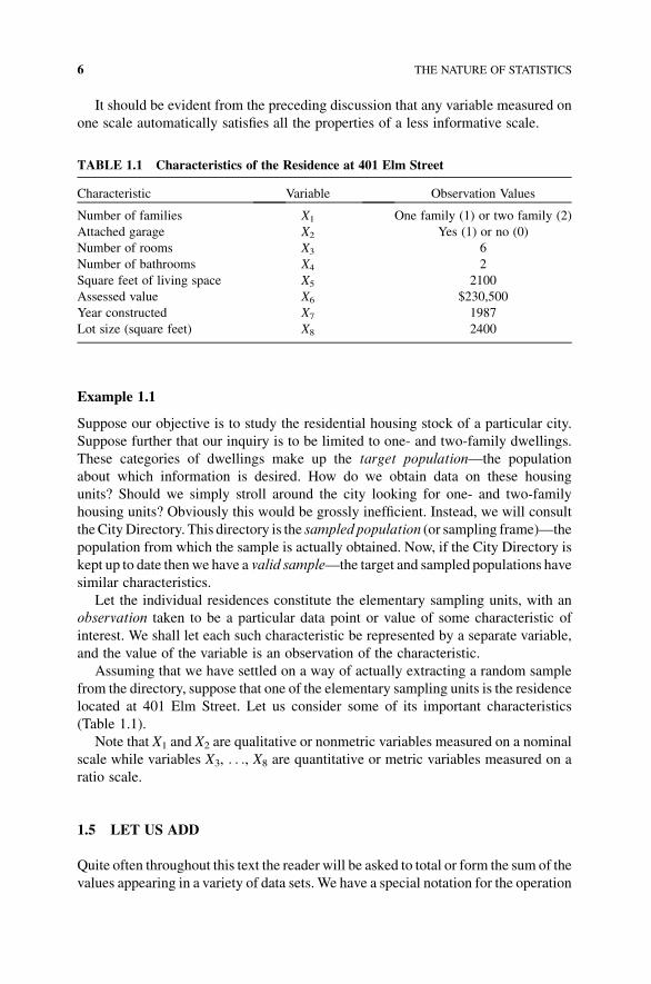
Example 1.1
Suppose our objective is to study the residential housing stock of a particular city.
Suppose further that our inquiry is to be limited to one- and two-family dwellings.
These categories of dwellings make up the target population—the population
about which information is desired. How do we obtain data on these housing
units? Should we simply stroll around the city looking for one- and two-family
housing units? Obviously this would be grossly inefficient. Instead, we will consult
theCityDirectory. This directory is the sampled population (or sampling frame)—the
population from which the sample is actually obtained. Now, if the City Directory is
kept up to date then we have a valid sample—the target and sampled populations have
similar characteristics.
Let the individual residences constitute the elementary sampling units, with an
observation taken to be a particular data point or value of some characteristic of
interest. We shall let each such characteristic be represented by a separate variable,
and the value of the variable is an observation of the characteristic.
Assuming that we have settled on a way of actually extracting a random sample
from the directory, suppose that one of the elementary sampling units is the residence
located at 401 Elm Street. Let us consider some of its important characteristics
(Table 1.1).
Note that X1 and X2 are qualitative or nonmetric variables measured on a nominal
scale while variables X3, . . ., X8 are quantitative or metric variables measured on a
ratio scale.
1.5 LET US ADD
Quite often throughout this text the reader will be asked to total or form the sum of the
values appearing in a variety of data sets. We have a special notation for the operation
TABLE 1.1 Characteristics of the Residence at 401 Elm Street
Characteristic Variable Observation Values
Number of families X1 One family (1) or two family (2)
Attached garage X2 Yes (1) or no (0)
Number of rooms X3 6
Number of bathrooms X4 2
Square feet of living space X5 2100
Assessed value X6 $230,500
Year constructed X7 1987
Lot size (square feet) X8 2400
6 THE NATURE OF STATISTICS
of addition. We will let the Greek capital sigma or S serve as our “summation sign.”
Specifically, for a variable X with values X1, X2, . . ., Xn,
X1 þ X2 þ � � � þ Xn ¼Xn
i¼1
Xi: ð1:1Þ
Here the right-hand side of this expression reads “the sum of all observations Xi as i
goes from 1 to n.” In this regard, S is termed an operator—it operates only on those
items having an i index, and the operation is addition.When it is to be understood that
we are to add over all i values, then Equation (1.1) can be rewritten simply as
X1 þ X2 þ � � � þ Xn ¼ SXi.
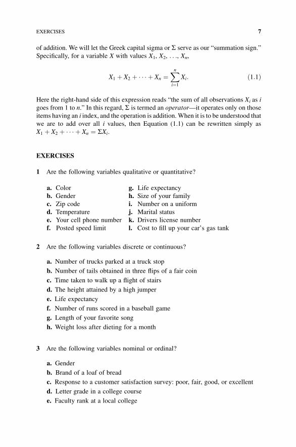
EXERCISES
1 Are the following variables qualitative or quantitative?
a. Color g. Life expectancy
b. Gender h. Size of your family
c. Zip code i. Number on a uniform
d. Temperature j. Marital status
e. Your cell phone number k. Drivers license number
f. Posted speed limit l. Cost to fill up your car’s gas tank
2 Are the following variables discrete or continuous?
a. Number of trucks parked at a truck stop
b. Number of tails obtained in three flips of a fair coin
c. Time taken to walk up a flight of stairs
d. The height attained by a high jumper
e. Life expectancy
f. Number of runs scored in a baseball game
g. Length of your favorite song
h. Weight loss after dieting for a month
3 Are the following variables nominal or ordinal?
a. Gender
b. Brand of a loaf of bread
c. Response to a customer satisfaction survey: poor, fair, good, or excellent
d. Letter grade in a college course
e. Faculty rank at a local college
EXERCISES 7
4 Are the following variables all measured on a ratio scale?
a. Cost of a new pair of shoes
b. A day’s wages for a laborer
c. Your house number
d. Porridge in the pot 9 days old
e. Your shoe size
f. An IQ score of 130
8 THE NATURE OF STATISTICS
2ANALYZING QUANTITATIVE DATA
2.1 IMPOSING ORDER
In this and the next chapter, we shall work in the area of descriptive statistics. As
indicated above, descriptive techniques serve to summarize data; we want to put the
data into a “readable form” or to “create order.” In doing so we can determine, for
instance, if a “pattern of behavior” emerges.
2.2 TABULAR AND GRAPHICAL TECHNIQUES: UNGROUPED DATA
Supposewe have a sample of n observations on somevariableX. This can bewritten as
X : X1; X2; . . . ; Xn or X : Xi; i ¼ 1; . . . ; n
Our first construct is what is called an absolute frequency distribution—it shows
the absolute frequencies with which the “different” values of a variable X occur in a
set of data, where absolute frequency (fj) is the number of times a particular value of
X is recorded.
Example 2.1
Let the n¼ 15 values of a variable X appear as
X : 1; 3; 1; 2; 4; 1; 3; 5; 6; 6; 4; 2; 3; 4; 3:
Statistical Inference: A Short Course, First Edition. Michael J. Panik.� 2012 John Wiley & Sons, Inc. Published 2012 by John Wiley & Sons, Inc.
9
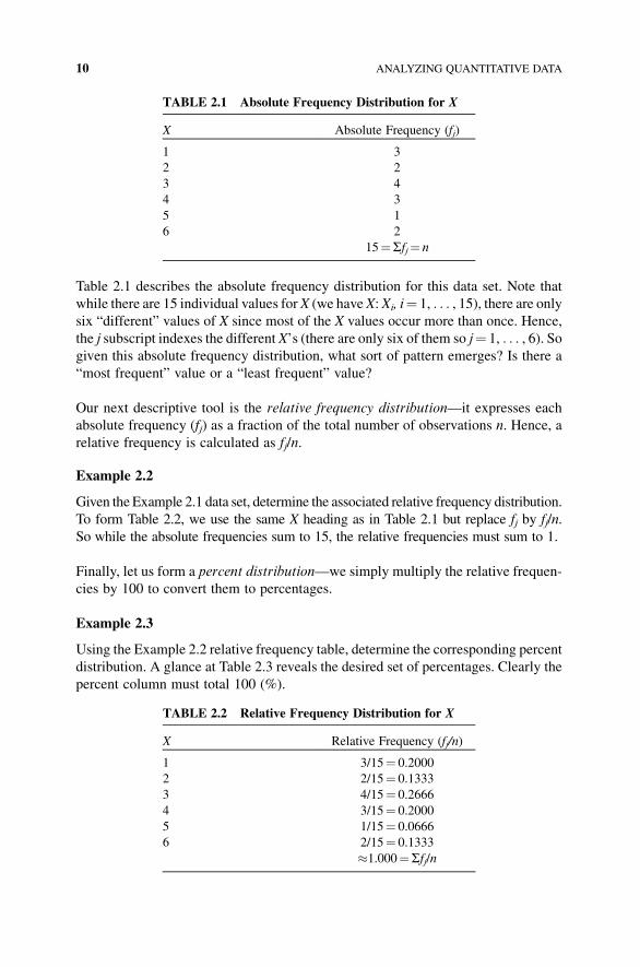
Table 2.1 describes the absolute frequency distribution for this data set. Note that
while there are 15 individual values forX (we haveX:Xi, i¼ 1, . . . , 15), there are onlysix “different” values of X since most of the X values occur more than once. Hence,
the j subscript indexes the different X’s (there are only six of them so j¼ 1, . . . , 6). Sogiven this absolute frequency distribution, what sort of pattern emerges? Is there a
“most frequent” value or a “least frequent” value?
Our next descriptive tool is the relative frequency distribution—it expresses each
absolute frequency (fj) as a fraction of the total number of observations n. Hence, a
relative frequency is calculated as fj/n.
Example 2.2
Given theExample 2.1 data set, determine the associated relative frequency distribution.
To form Table 2.2, we use the same X heading as in Table 2.1 but replace fj by fj/n.
So while the absolute frequencies sum to 15, the relative frequencies must sum to 1.
Finally, let us form a percent distribution—we simply multiply the relative frequen-
cies by 100 to convert them to percentages.
Example 2.3
Using the Example 2.2 relative frequency table, determine the corresponding percent
distribution. A glance at Table 2.3 reveals the desired set of percentages. Clearly the
percent column must total 100 (%).
TABLE 2.1 Absolute Frequency Distribution for X
X Absolute Frequency (fj)
1 3
2 2
3 4
4 3
5 1
6 2
15¼Sfj¼ n
TABLE 2.2 Relative Frequency Distribution for X
X Relative Frequency (fj/n)
1 3/15¼ 0.2000
2 2/15¼ 0.1333
3 4/15¼ 0.2666
4 3/15¼ 0.2000
5 1/15¼ 0.0666
6 2/15¼ 0.1333
�1.000¼Sfj/n
10 ANALYZING QUANTITATIVE DATA
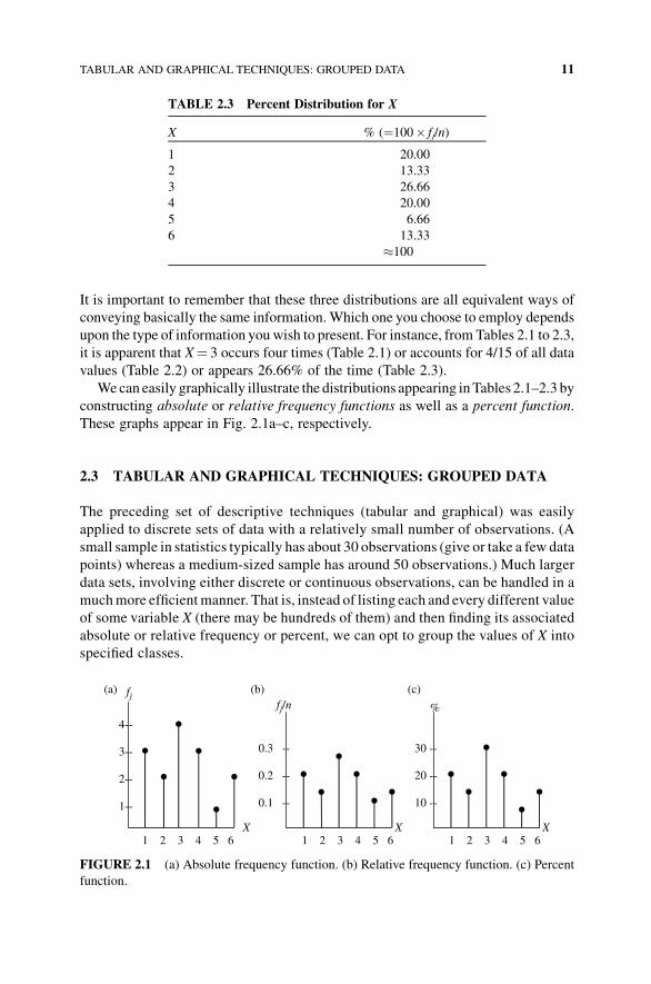
It is important to remember that these three distributions are all equivalent ways of
conveying basically the same information.Which one you choose to employ depends
upon the type of information you wish to present. For instance, from Tables 2.1 to 2.3,
it is apparent that X¼ 3 occurs four times (Table 2.1) or accounts for 4/15 of all data
values (Table 2.2) or appears 26.66% of the time (Table 2.3).
We can easily graphically illustrate the distributions appearing inTables 2.1–2.3 by
constructing absolute or relative frequency functions as well as a percent function.
These graphs appear in Fig. 2.1a–c, respectively.
2.3 TABULAR AND GRAPHICAL TECHNIQUES: GROUPED DATA
The preceding set of descriptive techniques (tabular and graphical) was easily
applied to discrete sets of data with a relatively small number of observations. (A
small sample in statistics typically has about 30 observations (give or take a few data
points) whereas a medium-sized sample has around 50 observations.) Much larger
data sets, involving either discrete or continuous observations, can be handled in a
muchmore efficientmanner. That is, instead of listing each and every different value
of some variable X (there may be hundreds of them) and then finding its associated
absolute or relative frequency or percent, we can opt to group the values of X into
specified classes.
TABLE 2.3 Percent Distribution for X
X % (¼100� fj/n)
1 20.00
2 13.33
3 26.66
4 20.00
5 6.66
6 13.33
�100
fjfj/n %
4--
0.3 -- 30 --3--
0.2 -- 20 --2--
0.1 -- 10 --1--
X X X1 2 3 4 5 6 1 2 3 4 5 6 1 2 3 4 5 6
(a) (b) (c)
FIGURE 2.1 (a) Absolute frequency function. (b) Relative frequency function. (c) Percent
function.
TABULAR AND GRAPHICAL TECHNIQUES: GROUPED DATA 11
Paralleling the above development of tabular and graphical methods, let us first
determine an absolute frequency distribution—it shows the absolute frequencies with
which the various values of a variableX are distributed among chosen classes. Here an
absolute frequency is now a class frequency—it is the number of items falling into a
given class.
The process of constructing this distribution consists of the following steps:
1. Choose the classes into which the data are to be grouped. Here, we must do the
following:
(a) Determine the number of classes.
(b) Specify the range of values each class is to cover.
2. Sort the observations into appropriate classes.
3. Count the number of items in each class so as to determine absolute class
frequencies.
While there are no hard and fast rules for carrying out step 1, certain guidelines or
“rules of thumb” can be offered. For instance, as follows:
1. Usually the number of classes ranges between 5 and 20 inclusive.
2. Obviouslyonemustchoosetheclassessothatallof thedatacanbeaccommodated.
3. Each Xi belongs to one and only one class (avoid overlapping classes).
4. The class intervals should be equal (the class interval is the length of a class).1
5. Try to avoid open-ended classes (e.g., the class “65 and over” is open ended).
6. The resulting distribution should have a single peak (i.e., we would like to be
able to identify a major point of concentration of data).
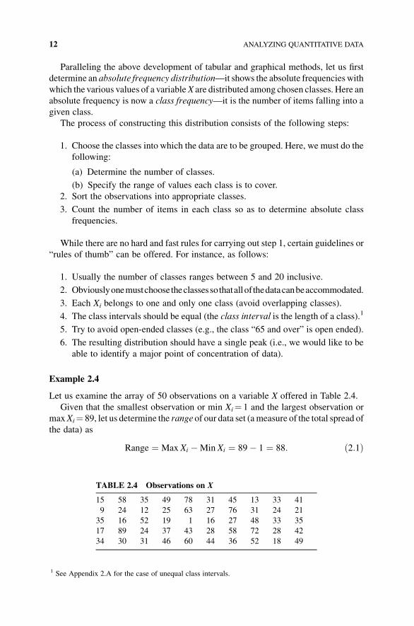
Example 2.4
Let us examine the array of 50 observations on a variable X offered in Table 2.4.
Given that the smallest observation or min Xi¼ 1 and the largest observation or
maxXi¼ 89, let us determine the range of our data set (ameasure of the total spread of
the data) as
Range ¼ Max Xi �Min Xi ¼ 89� 1 ¼ 88: ð2:1Þ
1 See Appendix 2.A for the case of unequal class intervals.
TABLE 2.4 Observations on X
15 58 35 49 78 31 45 13 33 41
9 24 12 25 63 27 76 31 24 21
35 16 52 19 1 16 27 48 33 35
17 89 24 37 43 28 58 72 28 42
34 30 31 46 60 44 36 52 18 49
12 ANALYZING QUANTITATIVE DATA
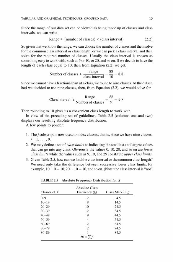
Since the range of our data set can be viewed as being made up of classes and class
intervals, we can write
Range � ðnumber of classesÞ � ðclass intervalÞ: ð2:2ÞSo given that we know the range, we can choose the number of classes and then solve
for the common class interval or class length; or we can pick a class interval and then
solve for the required number of classes. Usually the class interval is chosen as
something easy towork with, such as 5 or 10, or 20, and so on. If we decide to have the
length of each class equal to 10, then from Equation (2.2) we get,
Number of classes � range
class interval¼ 88
10¼ 8:8:
Sincewe cannot have a fractional part of a class, we round to nine classes. At the outset,
had we decided to use nine classes, then, from Equation (2.2), we would solve for
Class interval � Range
Number of classes¼ 88
9¼ 9:8:
Then rounding to 10 gives us a convenient class length to work with.
In view of the preceding set of guidelines, Table 2.5 (columns one and two)
displays our resulting absolute frequency distribution.
A few points to ponder:
1. The j subscript is now used to index classes, that is, since we have nine classes,
j¼ 1, . . . , 9.
2. We may define a set of class limits as indicating the smallest and largest values
that can go into any class. Obviously the values 0, 10, 20, and so on are lower
class limitswhile the values such as 9, 19, and 29 constitute upper class limits.
3. Given Table 2.5, how canwe find the class interval or the common class length?
We need only take the difference between successive lower class limits, for
example, 10� 0¼ 10, 20� 10¼ 10, and so on. (Note: the class interval is “not”
TABLE 2.5 Absolute Frequency Distribution for X
Classes of X
Absolute Class
Frequency (fj) Class Mark (mj)
0–9 2 4.5
10–19 8 14.5
20–29 10 24.5
30–39 12 34.5
40–49 9 44.5
50–59 4 54.5
60–69 2 64.5
70–79 2 74.5
80–89 1 84.5
50¼Pfj
TABULAR AND GRAPHICAL TECHNIQUES: GROUPED DATA 13
the difference between the upper and lower class limits of a given class, that is,
for the third class, 29� 20¼ 9$ class length¼ 10.)
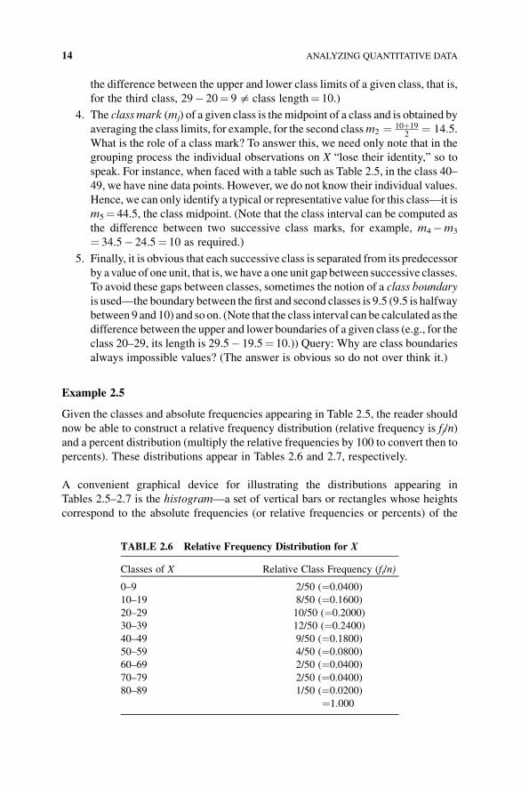
4. The class mark (mj) of a given class is themidpoint of a class and is obtained by
averaging the class limits, for example, for the second classm2 ¼ 10þ192
¼ 14:5.What is the role of a class mark? To answer this, we need only note that in the
grouping process the individual observations on X “lose their identity,” so to
speak. For instance, when faced with a table such as Table 2.5, in the class 40–
49, we have nine data points. However, we do not know their individual values.
Hence, we can only identify a typical or representative value for this class—it is
m5¼ 44.5, the class midpoint. (Note that the class interval can be computed as
the difference between two successive class marks, for example, m4�m3
¼ 34.5� 24.5¼ 10 as required.)
5. Finally, it is obvious that each successive class is separated from its predecessor
by a value of one unit, that is, we have a one unit gap between successive classes.
To avoid these gaps between classes, sometimes the notion of a class boundary
is used—the boundary between the first and second classes is 9.5 (9.5 is halfway
between 9 and 10) and so on. (Note that the class interval can be calculated as the
difference between the upper and lower boundaries of a given class (e.g., for the
class 20–29, its length is 29.5� 19.5¼ 10.)) Query: Why are class boundaries
always impossible values? (The answer is obvious so do not over think it.)
Example 2.5
Given the classes and absolute frequencies appearing in Table 2.5, the reader should
now be able to construct a relative frequency distribution (relative frequency is fj/n)
and a percent distribution (multiply the relative frequencies by 100 to convert then to
percents). These distributions appear in Tables 2.6 and 2.7, respectively.
A convenient graphical device for illustrating the distributions appearing in
Tables 2.5–2.7 is the histogram—a set of vertical bars or rectangles whose heights
correspond to the absolute frequencies (or relative frequencies or percents) of the
TABLE 2.6 Relative Frequency Distribution for X
Classes of X Relative Class Frequency (fi/n)
0–9 2/50 (¼0.0400)
10–19 8/50 (¼0.1600)
20–29 10/50 (¼0.2000)
30–39 12/50 (¼0.2400)
40–49 9/50 (¼0.1800)
50–59 4/50 (¼0.0800)
60–69 2/50 (¼0.0400)
70–79 2/50 (¼0.0400)
80–89 1/50 (¼0.0200)
¼1.000
14 ANALYZING QUANTITATIVE DATA
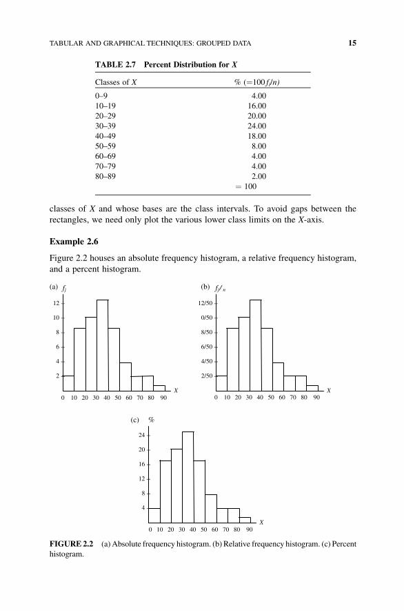
classes of X and whose bases are the class intervals. To avoid gaps between the
rectangles, we need only plot the various lower class limits on the X-axis.
Example 2.6
Figure 2.2 houses an absolute frequency histogram, a relative frequency histogram,
and a percent histogram.
TABLE 2.7 Percent Distribution for X
Classes of X % (¼100 fi/n)
0–9 4.00
10–19 16.00
20–29 20.00
30–39 24.00
40–49 18.00
50–59 8.00
60–69 4.00
70–79 4.00
80–89 2.00
¼ 100
fj
12 --
10 --
8 --
6 --
4 --
2 --
X 0 10 20 30 40 50 60 70 80 90
(a) f /j n
12/50 --
0/50 --
8/50 --
6/50 --
4/50 --
2/50 --
X 0 10 20 30 40 50 60 70 80 90
(b)
(c) %
24 --
20 --
16 --
12 --
8 --
4 --
X 0 10 20 30 40 50 60 70 80 90
FIGURE2.2 (a) Absolute frequency histogram. (b) Relative frequency histogram. (c) Percent
histogram.
TABULAR AND GRAPHICAL TECHNIQUES: GROUPED DATA 15
EXERCISES
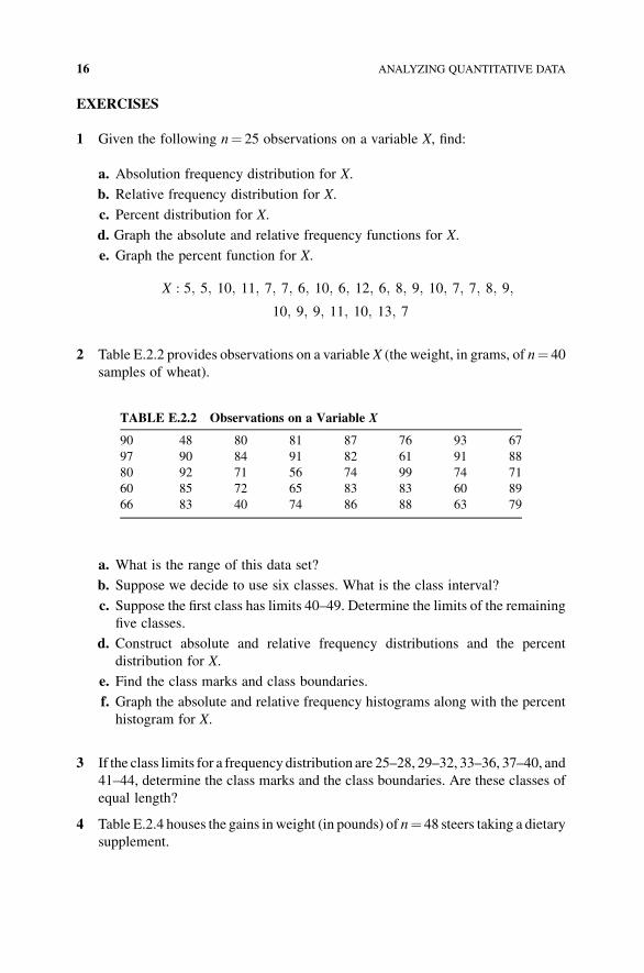
1 Given the following n¼ 25 observations on a variable X, find:
a. Absolution frequency distribution for X.
b. Relative frequency distribution for X.
c. Percent distribution for X.
d. Graph the absolute and relative frequency functions for X.
e. Graph the percent function for X.
X : 5; 5; 10; 11; 7; 7; 6; 10; 6; 12; 6; 8; 9; 10; 7; 7; 8; 9;
10; 9; 9; 11; 10; 13; 7
2 Table E.2.2 provides observations on a variable X (the weight, in grams, of n¼ 40
samples of wheat).
a. What is the range of this data set?
b. Suppose we decide to use six classes. What is the class interval?
c. Suppose the first class has limits 40–49. Determine the limits of the remaining
five classes.
d. Construct absolute and relative frequency distributions and the percent
distribution for X.
e. Find the class marks and class boundaries.
f. Graph the absolute and relative frequency histograms along with the percent
histogram for X.
3 If the class limits for a frequency distribution are 25–28, 29–32, 33–36, 37–40, and
41–44, determine the class marks and the class boundaries. Are these classes of
equal length?
4 Table E.2.4 houses the gains inweight (in pounds) of n¼ 48 steers taking a dietary
supplement.
TABLE E.2.2 Observations on a Variable X
90 48 80 81 87 76 93 67
97 90 84 91 82 61 91 88
80 92 71 56 74 99 74 71
60 85 72 65 83 83 60 89
66 83 40 74 86 88 63 79
16 ANALYZING QUANTITATIVE DATA
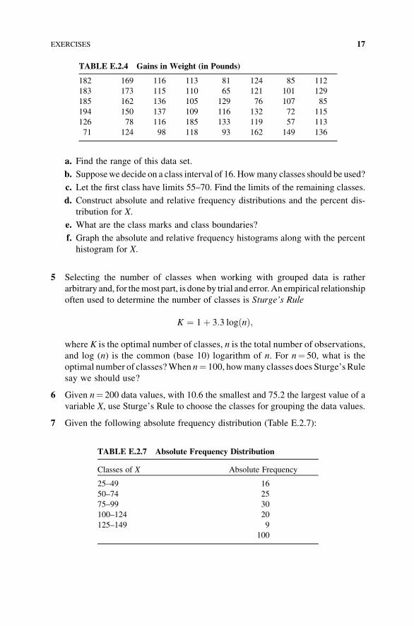
a. Find the range of this data set.
b. Supposewe decide on a class interval of 16. Howmany classes should be used?
c. Let the first class have limits 55–70. Find the limits of the remaining classes.
d. Construct absolute and relative frequency distributions and the percent dis-
tribution for X.
e. What are the class marks and class boundaries?
f. Graph the absolute and relative frequency histograms along with the percent
histogram for X.
5 Selecting the number of classes when working with grouped data is rather
arbitrary and, for themost part, is done by trial and error.An empirical relationship
often used to determine the number of classes is Sturge’s Rule
K ¼ 1þ 3:3 logðnÞ;
where K is the optimal number of classes, n is the total number of observations,
and log (n) is the common (base 10) logarithm of n. For n¼ 50, what is the
optimal number of classes?When n¼ 100, howmany classes does Sturge’s Rule
say we should use?
6 Given n¼ 200 data values, with 10.6 the smallest and 75.2 the largest value of a
variable X, use Sturge’s Rule to choose the classes for grouping the data values.
7 Given the following absolute frequency distribution (Table E.2.7):
TABLE E.2.4 Gains in Weight (in Pounds)
182 169 116 113 81 124 85 112
183 173 115 110 65 121 101 129
185 162 136 105 129 76 107 85
194 150 137 109 116 132 72 115
126 78 116 185 133 119 57 113
71 124 98 118 93 162 149 136
TABLE E.2.7 Absolute Frequency Distribution
Classes of X Absolute Frequency
25–49 16
50–74 25
75–99 30
100–124 20
125–149 9
100
EXERCISES 17
a. Determine the class marks and class boundaries. What is the class interval?
b. Determine the relative frequency and percent distributions.
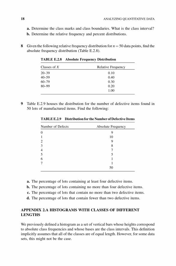
8 Given the following relative frequency distribution for n¼ 50 data points, find the
absolute frequency distribution (Table E.2.8).
9 Table E.2.9 houses the distribution for the number of defective items found in
50 lots of manufactured items. Find the following:
a. The percentage of lots containing at least four defective items.
b. The percentage of lots containing no more than four defective items.
c. The percentage of lots that contain no more than two defective items.
d. The percentage of lots that contain fewer than two defective items.
APPENDIX 2.A HISTOGRAMS WITH CLASSES OF DIFFERENT
LENGTHS
We previously defined a histogram as a set of vertical bars whose heights correspond
to absolute class frequencies and whose bases are the class intervals. This definition
implicitly assumes that all of the classes are of equal length. However, for some data
sets, this might not be the case.
TABLE E.2.8 Absolute Frequency Distribution
Classes of X Relative Frequency
20–39 0.10
40–59 0.40
60–79 0.30
80–99 0.20
1.00
TABLEE.2.9 Distribution for theNumber ofDefective Items
Number of Defects Absolute Frequency
0 9
1 10
2 9
3 8
4 7
5 5
6 1
7 1
50
18 ANALYZING QUANTITATIVE DATA
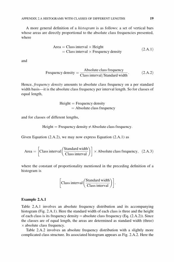
A more general definition of a histogram is as follows: a set of vertical bars
whose areas are directly proportional to the absolute class frequencies presented,
where
Area ¼ Class interval� Height
¼ Class interval� Frequency densityð2:A:1Þ
and
Frequency density ¼ Absolute class frequency
Class interval=Standard width: ð2:A:2Þ
Hence, frequency density amounts to absolute class frequency on a per standard
width basis—it is the absolute class frequency per interval length. So for classes of
equal length,
Height ¼ Frequency density
¼ Absolute class frequency
and for classes of different lengths,
Height ¼ Frequency density$Absolute class frequency:
Given Equation (2.A.2), we may now express Equation (2.A.1) as
Area ¼ Class intervalStandard width
Class interval
� �� �� Absolute class frequency; ð2:A:3Þ
where the constant of proportionality mentioned in the preceding definition of a
histogram is
Class intervalStandard width
Class interval
� �� �:
Example 2.A.1
Table 2.A.1 involves an absolute frequency distribution and its accompanying
histogram (Fig. 2.A.1). Here the standard width of each class is three and the height
of each class is its frequency density¼ absolute class frequency (Eq. (2.A.2)). Since
the classes are of equal length, the areas are determined as standard width (three)
� absolute class frequency.
Table 2.A.2 involves an absolute frequency distribution with a slightly more
complicated class structure. Its associated histogram appears as Fig. 2.A.2. Here the
APPENDIX 2.A HISTOGRAMS WITH CLASSES OF DIFFERENT LENGTHS 19
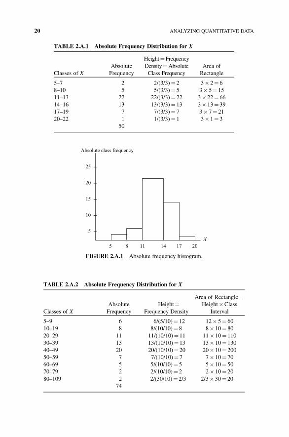
TABLE 2.A.1 Absolute Frequency Distribution for X
Classes of X
Absolute
Frequency
Height¼ Frequency
Density¼Absolute
Class Frequency
Area of
Rectangle
5–7 2 2/(3/3)¼ 2 3� 2¼ 6
8–10 5 5/(3/3)¼ 5 3� 5¼ 15
11–13 22 22/(3/3)¼ 22 3� 22¼ 66
14–16 13 13/(3/3)¼ 13 3� 13¼ 39
17–19 7 7/(3/3)¼ 7 3� 7¼ 21
20–22 1 1/(3/3)¼ 1 3� 1¼ 3
50
Absolute class frequency
25 --
20 --
15 --
10 --
5 --
X
5 8 11 14 17 20
FIGURE 2.A.1 Absolute frequency histogram.
TABLE 2.A.2 Absolute Frequency Distribution for X
Classes of X
Absolute
Frequency
Height¼Frequency Density
Area of Rectangle ¼Height�Class
Interval
5–9 6 6/(5/10)¼ 12 12� 5¼ 60
10–19 8 8/(10/10)¼ 8 8� 10¼ 80
20–29 11 11/(10/10)¼ 11 11� 10¼ 110
30–39 13 13/(10/10)¼ 13 13� 10¼ 130
40–49 20 20/(10/10)¼ 20 20� 10¼ 200
50–59 7 7/(10/10)¼ 7 7� 10¼ 70
60–69 5 5/(10/10)¼ 5 5� 10¼ 50
70–79 2 2/(10/10)¼ 2 2� 10¼ 20
80–109 2 2/(30/10)¼ 2/3 2/3� 30¼ 20
74
20 ANALYZING QUANTITATIVE DATA
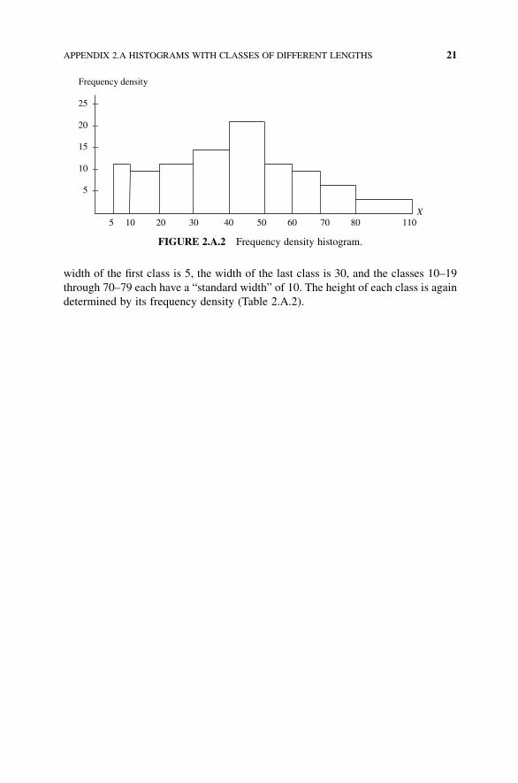
width of the first class is 5, the width of the last class is 30, and the classes 10–19
through 70–79 each have a “standard width” of 10. The height of each class is again
determined by its frequency density (Table 2.A.2).
Frequency density
25 --
20 --
15 --
10 --
5 --
X 5 10 20 30 40 50 60 70 80 110
FIGURE 2.A.2 Frequency density histogram.
APPENDIX 2.A HISTOGRAMS WITH CLASSES OF DIFFERENT LENGTHS 21
3DESCRIPTIVE CHARACTERISTICSOF QUANTITATIVE DATA
3.1 THE SEARCH FOR SUMMARY CHARACTERISTICS
Up to this point in our data analysis, we have been working with the entire set of
observations, either in tabular form (e.g., an absolute frequency distribution) or in
graphical form (e.g., an absolute frequency function or an absolute frequency
histogram). Is there a more efficient way of squeezing information out of a set of
quantitative data? As one might have anticipated, the answer is yes. Instead of
working with the entire mass of data in the form of a table or graph, let us determine
concise summary characteristics of our variable X, which are indicative of the
properties of the data set itself.
If we are working with a population of X values, then these descriptive measures
will be termed “parameters.” Hence a parameter is any descriptive measure of a
population. But if we are dealing with a sample of X values drawn from the
X population, then these descriptive measures will be called “statistics.” Thus a
statistic is any descriptive measure of a sample. (You now know what this book is
ultimately all about—you are going to study descriptivemeasures of samples.) As we
shall see later on, statistics are used tomeasure or estimate (unknown) parameters. For
any population, parameters are constants. However, the value of a statistic is variable;
its value depends upon the particular sample chosen, that is, it is sample sensitive.
(This is why sampling error is an important factor in estimating a parameter.)
Statistical Inference: A Short Course, First Edition. Michael J. Panik.� 2012 John Wiley & Sons, Inc. Published 2012 by John Wiley & Sons, Inc.
22
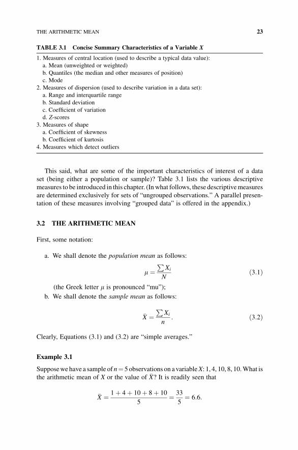
This said, what are some of the important characteristics of interest of a data
set (being either a population or sample)? Table 3.1 lists the various descriptive
measures to be introduced in this chapter. (Inwhat follows, these descriptivemeasures
are determined exclusively for sets of “ungrouped observations.” A parallel presen-
tation of these measures involving “grouped data” is offered in the appendix.)
3.2 THE ARITHMETIC MEAN
First, some notation:
a. We shall denote the population mean as follows:
m ¼P
Xi
Nð3:1Þ
(the Greek letter m is pronounced “mu”);
b. We shall denote the sample mean as follows:
�X ¼P
Xi
n: ð3:2Þ
Clearly, Equations (3.1) and (3.2) are “simple averages.”
Example 3.1
Supposewe have a sample of n¼ 5 observations on avariableX: 1, 4, 10, 8, 10.What is
the arithmetic mean of X or the value of �X? It is readily seen that
�X ¼ 1þ 4þ 10þ 8þ 10
5¼ 33
5¼ 6:6:
TABLE 3.1 Concise Summary Characteristics of a Variable X
1. Measures of central location (used to describe a typical data value):
a. Mean (unweighted or weighted)
b. Quantiles (the median and other measures of position)
c. Mode
2. Measures of dispersion (used to describe variation in a data set):
a. Range and interquartile range
b. Standard deviation
c. Coefficient of variation
d. Z-scores
3. Measures of shape
a. Coefficient of skewness
b. Coefficient of kurtosis
4. Measures which detect outliers
THE ARITHMETIC MEAN 23
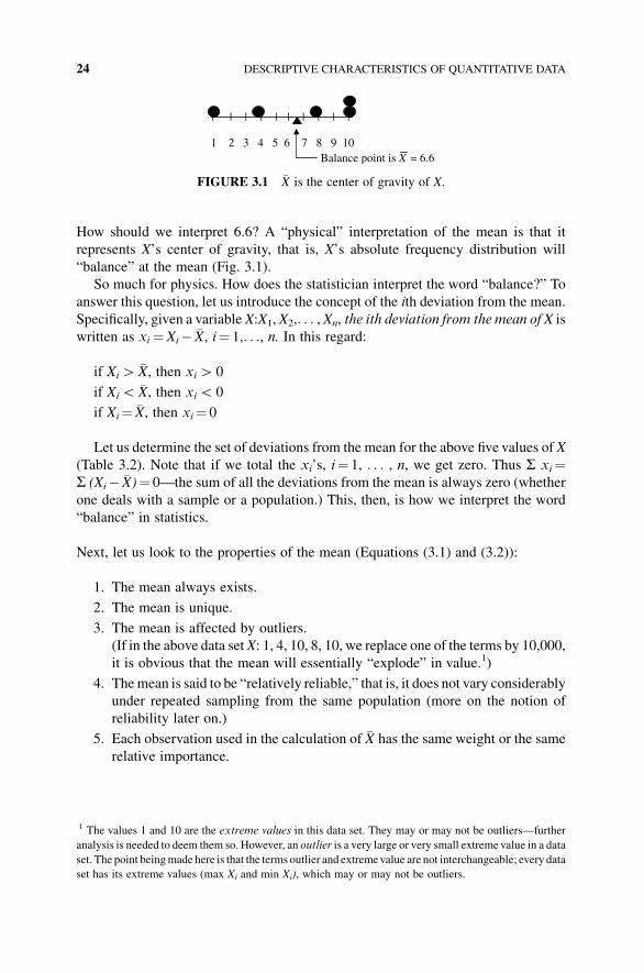
How should we interpret 6.6? A “physical” interpretation of the mean is that it
represents X’s center of gravity, that is, X’s absolute frequency distribution will
“balance” at the mean (Fig. 3.1).
So much for physics. How does the statistician interpret the word “balance?” To
answer this question, let us introduce the concept of the ith deviation from the mean.
Specifically, given a variable X:X1, X2,. . . , Xn, the ith deviation from the mean of X is
written as xi ¼Xi� �X, i¼ 1,. . ., n. In this regard:
if XiH �X, then xiH 0
if XiG �X, then xiG 0
if Xi¼ �X, then xi¼ 0
Let us determine the set of deviations from the mean for the above five values of X
(Table 3.2). Note that if we total the xi’s, i¼ 1, . . . , n, we get zero. Thus S xi¼S (Xi� �X)¼ 0—the sum of all the deviations from the mean is always zero (whether
one deals with a sample or a population.) This, then, is how we interpret the word
“balance” in statistics.
Next, let us look to the properties of the mean (Equations (3.1) and (3.2)):
1. The mean always exists.
2. The mean is unique.
3. The mean is affected by outliers.
(If in the above data set X: 1, 4, 10, 8, 10, we replace one of the terms by 10,000,
it is obvious that the mean will essentially “explode” in value.1)
4. Themean is said to be “relatively reliable,” that is, it does not vary considerably
under repeated sampling from the same population (more on the notion of
reliability later on.)
5. Each observation used in the calculation of �X has the same weight or the same
relative importance.
|
1 2 3 4 5 6 7 8 9 10 Balance point is X = 6.6
| | | | | | | ||
FIGURE 3.1 �X is the center of gravity of X.
1 The values 1 and 10 are the extreme values in this data set. They may or may not be outliers—further
analysis is needed to deem them so. However, an outlier is a very large or very small extreme value in a data
set. The point beingmade here is that the terms outlier and extremevalue are not interchangeable; every data
set has its extreme values (max Xi and min Xi), which may or may not be outliers.
24 DESCRIPTIVE CHARACTERISTICS OF QUANTITATIVE DATA
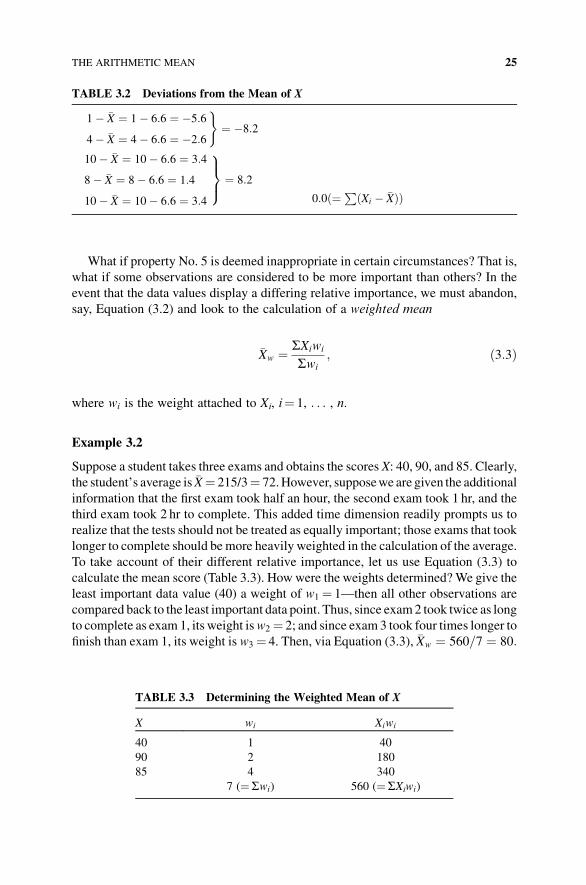
What if property No. 5 is deemed inappropriate in certain circumstances? That is,
what if some observations are considered to be more important than others? In the
event that the data values display a differing relative importance, we must abandon,
say, Equation (3.2) and look to the calculation of a weighted mean
�Xw ¼ SXiwi
Swi
; ð3:3Þ
where wi is the weight attached to Xi, i¼ 1, . . . , n.
Example 3.2
Suppose a student takes three exams and obtains the scores X: 40, 90, and 85. Clearly,
the student’s average is �X¼ 215/3¼ 72.However, supposewe are given the additional
information that the first exam took half an hour, the second exam took 1 hr, and the
third exam took 2 hr to complete. This added time dimension readily prompts us to
realize that the tests should not be treated as equally important; those exams that took
longer to complete should bemore heavily weighted in the calculation of the average.
To take account of their different relative importance, let us use Equation (3.3) to
calculate the mean score (Table 3.3). How were the weights determined?We give the
least important data value (40) a weight of w1 ¼ 1—then all other observations are
compared back to the least important data point. Thus, since exam2 took twice as long
to complete as exam 1, its weight isw2 ¼ 2; and since exam3 took four times longer to
finish than exam 1, its weight is w3 ¼ 4. Then, via Equation (3.3), �Xw ¼ 560=7 ¼ 80:
TABLE 3.2 Deviations from the Mean of X
1� �X ¼ 1� 6:6 ¼ �5:6
4� �X ¼ 4� 6:6 ¼ �2:6
)¼ �8:2
10� �X ¼ 10� 6:6 ¼ 3:4
8� �X ¼ 8� 6:6 ¼ 1:4
10� �X ¼ 10� 6:6 ¼ 3:4
9>=
>;¼ 8:2
0:0ð¼PðXi � �XÞÞ
TABLE 3.3 Determining the Weighted Mean of X
X wi Xiwi
40 1 40
90 2 180
85 4 340
7 (¼Swi) 560 (¼SXiwi)
THE ARITHMETIC MEAN 25
Why is theweighted average higher than the unweighted average? Because the person
did better on those exams that carried the larger weights. (What if the second exam
took 1 hr and 15min to complete and the third exam was finished in 2 hr and 30 min?
The reader should be able to determine that the revised set of weights is now:
w1 ¼ 1;w2 ¼ 2:5; and w3 ¼ 5:)
3.3 THE MEDIAN
For a variable X (representing a sample or a population), let us define themedian of X
as the value that divides the observations on X into two equal parts; it is a positional
value—half of the observations on X lie below the median, and half lie above the
median. Since there is no standard notation in statistics for themedian, we shall invent
our own: the population median will be denoted as “Med;” the sample median will
appear as “med.”
Since the median is not a calculated value (as was the mean) but only a positional
value that locates the middle of our data set, we need some rules for determining the
median. To this end, we have rules for finding the median:
1. Arrange the observations on a variable X in an increasing sequence.
2. (a) For an odd number of observations, there is always a middle term whose
value is the median.
(b) For an evennumber of observations, there is no specificmiddle term.Hence
take as the median the average of the two middle terms.
Note that for either case 2a or 2b, the median is the term that occupies the position
ðnþ 1Þ=2 (or ðN þ 1Þ=2) in the increasing sequence of data values.
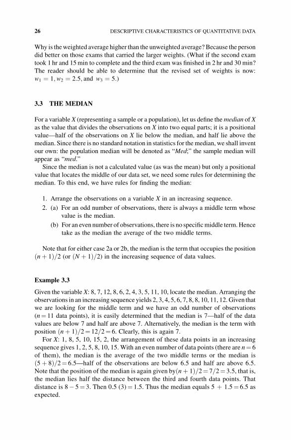
Example 3.3
Given the variable X: 8, 7, 12, 8, 6, 2, 4, 3, 5, 11, 10, locate the median. Arranging the
observations in an increasing sequence yields 2, 3, 4, 5, 6, 7, 8, 8, 10, 11, 12. Given that
we are looking for the middle term and we have an odd number of observations
(n¼ 11 data points), it is easily determined that the median is 7—half of the data
values are below 7 and half are above 7. Alternatively, the median is the term with
position ðnþ 1Þ=2¼ 12=2¼ 6. Clearly, this is again 7.
For X: 1, 8, 5, 10, 15, 2, the arrangement of these data points in an increasing
sequence gives 1, 2, 5, 8, 10, 15. With an even number of data points (there are n¼ 6
of them), the median is the average of the two middle terms or the median is
ð5þ 8Þ=2¼ 6.5—half of the observations are below 6.5 and half are above 6.5.
Note that the position of the median is again given byðnþ 1Þ=2¼ 7=2¼ 3.5, that is,
the median lies half the distance between the third and fourth data points. That
distance is 8� 5¼ 3. Then 0.5 (3)¼ 1.5. Thus the median equals 5 þ 1.5¼ 6.5 as
expected.
26 DESCRIPTIVE CHARACTERISTICS OF QUANTITATIVE DATA
Looking to the properties of the median:
1. The median may or may not equal the mean.
2. The median always exists.
3. The median is unique.
4. The median is not affected by outliers (for X: 1, 8, 5, 10, 15, 2, if 15 is replaced
by 1000, the median is still 6.5).
3.4 THE MODE
The mode of X is the value that occurs with the highest frequency; it is the most
common ormost probable value ofX. Let us denote the populationmode as “Mo;” the
sample mode will appear as “mo.”
Example 3.4
For the sample data set X: 1, 2, 4, 4, 5, the modal value is mo¼ 4 (its frequency is
two); for the variable Y: 1, 2, 4, 4, 5, 6, 6, 9, there are twomodes—4 and 6 (Y is thus a
bimodal variable); and for Z: 1, 2, 3, 7, 9, 11, there is no mode (no one value appears
more often than any other).
For the properties of the mode:
1. The mode may or may not equal the mean and median.
2. The mode may not exist.
3. If the mode exists, it may not be unique.
4. The mode is not affected by outliers (for the data set X: 1, 2, 4, 4, 5, if 5 is
replaced by 1000, the mode is still four).
5. The mode always corresponds to one of the actual values of a variable X
We next turn to measures of dispersion or variation within a data set. Here we are
attempting to get a numerical measure of the spread or scatter of the values of a
variable X along the horizontal axis.
3.5 THE RANGE
We previously defined the range of a variable X as range¼max Xi�min Xi. Clearly,
the range is a measure of the total spread of the data. However, knowing the total
spread of the data values tells us nothing about what is going on between the extremes
of max Xi and min Xi. To specify a more appealing measure of dispersion, let us
consider the spread or scatter of the data points about the mean. In particular, let us
consider the “average variability about the mean.” This then takes us to the concept of
the standard deviation of a variable X.
THE RANGE 27
3.6 THE STANDARD DEVIATION
We previously denoted the ith deviation from the (sample) mean as Xi � �X. Since thesumof all the deviations from themean is zero, it is evident that oneway to circumvent
the issue of the sign of the difference Xi � �X is to square it. Then all of these squared
deviations from the mean are nonnegative.
Supposewe have a population ofX values orX:X1,X2, . . . ,XN. Then we can define
the variance of X as follows:
s2 ¼ SðXi � mÞ2N
; ð3:4Þ
that is, the population variance of X is the average of the squared deviations from
the mean of X or from m. Since the variance of any variable is expressed in terms of
(units of X)2 (e.g., if X is measured in “inches,” then s2 is expressed in terms of
“inches2”), a more convenient way of assessing variability about m is to work with
the standard deviation of X, which is defined as the positive square root of the
variance of X or
s ¼ffiffiffiffiffiffiffiffiffiffiffiffiffiffiffiffiffiffiffiffiffiffiSðXi � mÞ2
N
s
¼ffiffiffiffiffiffiffiffiffiffiffiffiffiffiffiffiffiffiffiSX2
i
N� m2
r: ð3:5Þ
Here s is expressed in the original units of X.
If we have a sample of observations on X or X: X1, X2, . . . , Xn, then the sample
variance of X is denoted as
s2 ¼ SðXi � �XÞ2n� 1
ð3:6Þ
and the (sample) standard deviation of X is
s ¼ffiffiffiffiffiffiffiffiffiffiffiffiffiffiffiffiffiffiffiffiffiffiSðXi � �XÞ2
n� 1
s
¼ffiffiffiffiffiffiffiffiffiffiffiffiffiffiffiffiffiffiffiffiffiffiffiffiffiffiffiffiffiffiffiffiffiffiSX2
i
n� 1� ðSXiÞ2nðn� 1Þ
s
: ð3:7Þ
Here too s is measured in the same units as X. (It is important to remember that, in
Equation (3.7),SX2i is a “sumof squares”while ðSXiÞ2 is the “square of a sum.” These
quantities are different entities and thus are not equal or interchangeable expressions.)
Note that in Equations (3.6) and (3.7), we have n – 1 in the denominator instead of n
itself. Here dividing by n� 1 is termed a correction for degrees of freedom (denoted
d.f.). We may view degrees of freedom as the number of independent observations
remaining in the sample, that is, it is the sample size n less the number of prior
28 DESCRIPTIVE CHARACTERISTICS OF QUANTITATIVE DATA
estimatesmade [�Xis our estimate ofm in Equation (3.6)].2 (Also, ifwe had divided by ninstead of n� 1, then Equation (3.6) would provide us with what is called a “biased”
estimator for s2. More on this point later.)
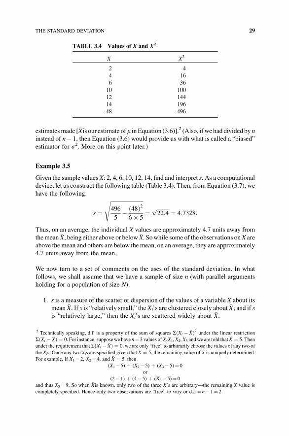
Example 3.5
Given the sample values X: 2, 4, 6, 10, 12, 14, find and interpret s. As a computational
device, let us construct the following table (Table 3.4). Then, from Equation (3.7), we
have the following:
s ¼ffiffiffiffiffiffiffiffiffiffiffiffiffiffiffiffiffiffiffiffiffiffiffiffi496
5� ð48Þ26� 5
s
¼ffiffiffiffiffiffiffiffiffi22:4
p¼ 4:7328:
Thus, on an average, the individual X values are approximately 4.7 units away from
themean �X, being either above or below �X. Sowhile some of the observations onX are
above themean and others are below themean, on an average, they are approximately
4.7 units away from the mean.
We now turn to a set of comments on the uses of the standard deviation. In what
follows, we shall assume that we have a sample of size n (with parallel arguments
holding for a population of size N):
1. s is a measure of the scatter or dispersion of the values of a variable X about its
mean �X. If s is “relatively small,” the Xi’s are clustered closely about �X; and if sis “relatively large,” then the Xi’s are scattered widely about �X.
TABLE 3.4 Values of X and X2
X X2
2 4
4 16
6 36
10 100
12 144
14 196
48 496
2 Technically speaking, d.f. is a property of the sum of squares SðXi � �XÞ2 under the linear restriction
SðXi � �XÞ ¼ 0. For instance, supposewe have n¼ 3 values ofX:X1,X2,X3 andwe are told that �X ¼ 5. Then
under the requirement thatSðXi � �XÞ ¼ 0, we are only “free” to arbitrarily choose the values of any two of
the Xis. Once any two Xis are specified given that �X ¼ 5, the remaining value of X is uniquely determined.
For example, if X1¼ 2, X2¼ 4, and �X ¼ 5, then
(X1� 5) þ (X2� 5) þ (X3� 5)¼ 0
or
(2� 1) þ (4� 5) þ (X3� 5)¼ 0
and thus X3¼ 9. So when �Xis known, only two of the three X’s are arbitrary—the remaining X value is
completely specified. Hence only two observations are “free” to vary or d.f.¼ n� 1¼ 2.
THE STANDARD DEVIATION 29
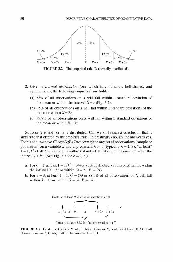
2. Given a normal distribution (one which is continuous, bell-shaped, and
symmetrical), the following empirical rule holds:
(a) 68% of all observations on X will fall within 1 standard deviation of
the mean or within the interval �X� s (Fig. 3.2).
(b) 95% of all observations on X will fall within 2 standard deviations of the
mean or within �X� 2s.
(c) 99.7% of all observations on X will fall within 3 standard deviations of
the mean or within �X� 3s.
Suppose X is not normally distributed. Can we still reach a conclusion that is
similar to that offered by the empirical rule? Interestingly enough, the answer is yes.
To this end, we have Chebysheff’s Theorem: given any set of observations (sample or
population) on a variable X and any constant kH 1 (typically k¼ 2, 3), “at least”
1� 1=k2 of all X values will lie within k standard deviations of the mean or within the
interval �X� ks. (See Fig. 3.3 for k¼ 2, 3.)
a. For k¼ 2, at least 1� 1=k2 ¼ 3/4 or 75% of all observations on Xwill lie within
the interval �X� 2s or within (�X� 2s, �X þ 2s).
b. For k¼ 3, at least 1� 1=k2 ¼ 8/9 or 88.9% of all observations on X will fall
within �X� 3s or within (�X� 3s, �X þ 3s).
Contains at least 75% of all observations on X
X
X – 3s X – 2s X X + 2s X + 3s
Contains at least 88.9% of all observations on X
FIGURE 3.3 Contains at least 75% of all observations on X; contains at least 88.9% of all
observations on X; Chebysheff’s Theorem for k¼ 2, 3.
X – 3s– X – 2s– X + 2s X + 3s–X – s– X + s–X–
0.15% 0.15%
2.35% 2.35%13.5% 13.5%
34% 34%
FIGURE 3.2 The empirical rule (X normally distributed).
30 DESCRIPTIVE CHARACTERISTICS OF QUANTITATIVE DATA
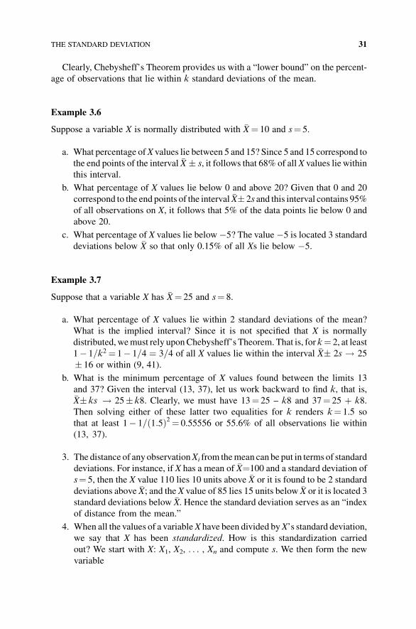
Clearly, Chebysheff’s Theorem provides us with a “lower bound” on the percent-
age of observations that lie within k standard deviations of the mean.
Example 3.6
Suppose a variable X is normally distributed with �X¼ 10 and s¼ 5.
a. What percentage ofX values lie between 5 and 15? Since 5 and 15 correspond to
the end points of the interval �X � s, it follows that 68% of all X values lie within
this interval.
b. What percentage of X values lie below 0 and above 20? Given that 0 and 20
correspond to the end points of the interval �X� 2s and this interval contains 95%
of all observations on X, it follows that 5% of the data points lie below 0 and
above 20.
c. What percentage of X values lie below�5? The value�5 is located 3 standard
deviations below �X so that only 0.15% of all Xs lie below �5.
Example 3.7
Suppose that a variable X has �X¼ 25 and s¼ 8.
a. What percentage of X values lie within 2 standard deviations of the mean?
What is the implied interval? Since it is not specified that X is normally
distributed, wemust rely uponChebysheff’s Theorem. That is, for k¼ 2, at least
1� 1=k2 ¼ 1� 1=4 ¼ 3=4 of all X values lie within the interval �X� 2s ! 25
� 16 or within (9, 41).
b. What is the minimum percentage of X values found between the limits 13
and 37? Given the interval (13, 37), let us work backward to find k, that is,�X� ks ! 25� k8. Clearly, we must have 13¼ 25 – k8 and 37¼ 25 þ k8.
Then solving either of these latter two equalities for k renders k¼ 1.5 so
that at least 1� 1=ð1:5Þ2 ¼ 0.55556 or 55.6% of all observations lie within
(13, 37).
3. The distance of anyobservationXi from themean can be put in terms of standard
deviations. For instance, if X has a mean of �X¼100 and a standard deviation of
s¼ 5, then the X value 110 lies 10 units above �X or it is found to be 2 standard
deviations above �X; and the X value of 85 lies 15 units below �X or it is located 3
standard deviations below �X. Hence the standard deviation serves as an “indexof distance from the mean.”
4. When all the values of a variableX have been divided byX’s standard deviation,
we say that X has been standardized. How is this standardization carried
out? We start with X: X1, X2, . . . , Xn and compute s. We then form the new
variable
THE STANDARD DEVIATION 31
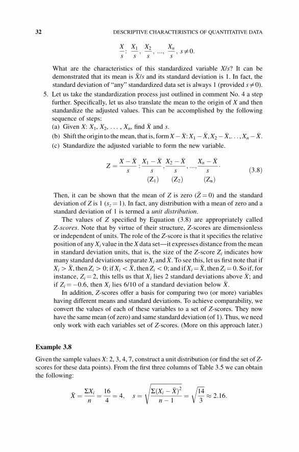
X
s:X1
s;X2
s; :::;
Xn
s; s$0:
What are the characteristics of this standardized variable X/s? It can be
demonstrated that its mean is �X/s and its standard deviation is 1. In fact, the
standard deviation of “any” standardized data set is always 1 (provided s$0).
5. Let us take the standardization process just outlined in comment No. 4 a step
further. Specifically, let us also translate the mean to the origin of X and then
standardize the adjusted values. This can be accomplished by the following
sequence of steps:
(a) Given X: X1, X2, . . . , Xn, find �X and s.
(b) Shift the origin to themean, that is, formX� �X:X1� �X,X2� �X,. . . ,Xn� �X:
(c) Standardize the adjusted variable to form the new variable.
Z ¼ X � �X
s:X1 � �X
s;X2 � �X
s; :::;
Xn � �X
s
Z1ð Þ Z2ð Þ Znð Þ
: ð3:8Þ
Then, it can be shown that the mean of Z is zero (�Z¼ 0) and the standard
deviation of Z is 1 (sz¼ 1). In fact, any distribution with a mean of zero and a
standard deviation of 1 is termed a unit distribution.
The values of Z specified by Equation (3.8) are appropriately called
Z-scores. Note that by virtue of their structure, Z-scores are dimensionless
or independent of units. The role of the Z-score is that it specifies the relative
position of anyXi value in theX data set—it expresses distance from themean
in standard deviation units, that is, the size of the Z-score Zi indicates how
many standard deviations separate Xi and �X. To see this, let us first note that ifXiH �X, then ZiH 0; ifXiG �X, then ZiG 0; and ifXi¼ �X, then Zi¼ 0. So if, for
instance, Zi¼ 2, this tells us that Xi lies 2 standard deviations above �X; andif Zi¼�0.6, then Xi lies 6/10 of a standard deviation below �X:
In addition, Z-scores offer a basis for comparing two (or more) variables
having different means and standard deviations. To achieve comparability, we
convert the values of each of these variables to a set of Z-scores. They now
have the samemean (of zero) and same standard deviation (of 1). Thus, we need
only work with each variables set of Z-scores. (More on this approach later.)
Example 3.8
Given the sample values X: 2, 3, 4, 7, construct a unit distribution (or find the set of Z-
scores for these data points). From the first three columns of Table 3.5 we can obtain
the following:
�X ¼ SXi
n¼ 16
4¼ 4; s ¼
ffiffiffiffiffiffiffiffiffiffiffiffiffiffiffiffiffiffiffiffiffiffiSðXi � �XÞ2
n� 1
s
¼ffiffiffiffiffi14
3
r� 2:16:
32 DESCRIPTIVE CHARACTERISTICS OF QUANTITATIVE DATA
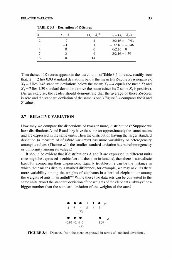
Then the set of Z-scores appears in the last column of Table 3.5. It is now readily seen
that: X1¼ 2 lies 0.93 standard deviations below the mean (its Z-score Z1 is negative);
X2¼ 3 lies 0.46 standard deviations below the mean; X3¼ 4 equals the mean �X; andX4¼ 7 lies 1.39 standard deviations above the mean (since its Z-score Z4 is positive).
(As an exercise, the reader should demonstrate that the average of these Z-scores
is zero and the standard deviation of the same is one.) Figure 3.4 compares the X and
Z values.
3.7 RELATIVE VARIATION
How may we compare the dispersions of two (or more) distributions? Suppose we
have distributionsA andB and they have the same (or approximately the same)means
and are expressed in the same units. Then the distribution having the larger standard
deviation (a measure of absolute variation) has more variability or heterogeneity
among its values. (The onewith the smaller standard deviation hasmore homogeneity
or uniformity among its values.)
It should be evident that if distributions A and B are expressed in different units
(onemight be expressed in cubic feet and the other in lumens), then there is no realistic
basis for comparing their dispersions. Equally troublesome can be the instance in
which their means display a marked difference, for example, we may ask: “is there
more variability among the weights of elephants in a herd of elephants or among
the weights of ants in an anthill?” While these two data sets can be converted to the
same units, won’t the standard deviation of theweights of the elephants “always” be a
bigger number than the standard deviation of the weights of the ants?
TABLE 3.5 Derivation of Z-Scores
X Xi� �X (Xi� �X)2 Zi¼ (Xi� �X)/s
2 �2 4 �2/2.16¼�0.93
3 �1 1 �1/2.16¼�0.46
4 0 0 0/2.16¼ 0
7 3 9 3/2.16¼ 1.39
16 0 14
X2 3 4 5 6 7
(X )
Z–0.93 –0.46 0 1.39
(Z )
FIGURE 3.4 Distance from the mean expressed in terms of standard deviations.
RELATIVE VARIATION 33
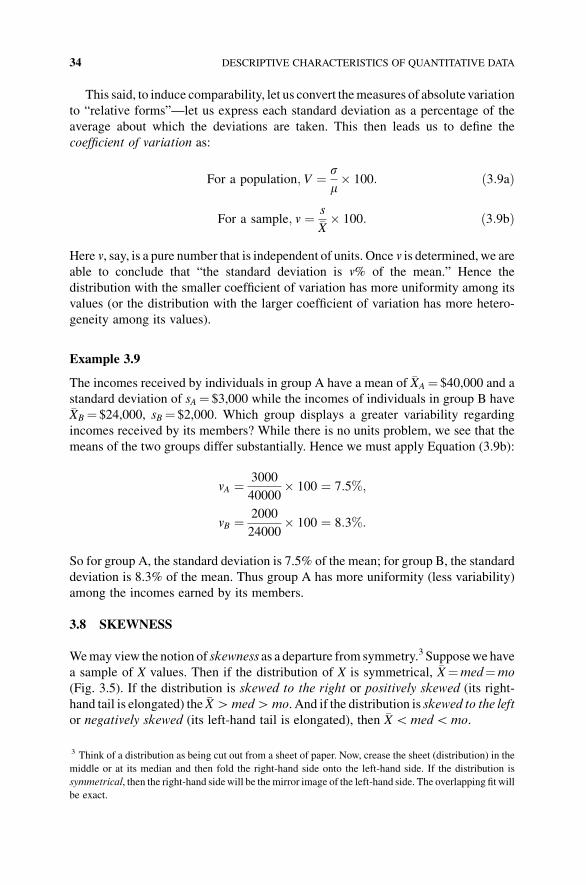
This said, to induce comparability, let us convert themeasures of absolute variation
to “relative forms”—let us express each standard deviation as a percentage of the
average about which the deviations are taken. This then leads us to define the
coefficient of variation as:
For a population; V ¼ sm� 100: ð3:9aÞ
For a sample; v ¼ s�X� 100: ð3:9bÞ
Here v, say, is a pure number that is independent of units. Once v is determined, we are
able to conclude that “the standard deviation is v% of the mean.” Hence the
distribution with the smaller coefficient of variation has more uniformity among its
values (or the distribution with the larger coefficient of variation has more hetero-
geneity among its values).
Example 3.9
The incomes received by individuals in group A have a mean of �XA ¼ $40,000 and a
standard deviation of sA ¼ $3,000 while the incomes of individuals in group B have�XB ¼ $24,000, sB ¼ $2,000. Which group displays a greater variability regarding
incomes received by its members? While there is no units problem, we see that the
means of the two groups differ substantially. Hence we must apply Equation (3.9b):
vA ¼ 3000
40000� 100 ¼ 7:5%;
vB ¼ 2000
24000� 100 ¼ 8:3%:
So for group A, the standard deviation is 7.5% of the mean; for group B, the standard
deviation is 8.3% of the mean. Thus group A has more uniformity (less variability)
among the incomes earned by its members.
3.8 SKEWNESS
Wemay view the notion of skewness as a departure from symmetry.3 Supposewe have
a sample of X values. Then if the distribution of X is symmetrical, �X¼med¼mo
(Fig. 3.5). If the distribution is skewed to the right or positively skewed (its right-
hand tail is elongated) the �XHmedHmo. And if the distribution is skewed to the left
or negatively skewed (its left-hand tail is elongated), then �XGmedGmo.
3 Think of a distribution as being cut out from a sheet of paper. Now, crease the sheet (distribution) in the
middle or at its median and then fold the right-hand side onto the left-hand side. If the distribution is
symmetrical, then the right-hand sidewill be themirror image of the left-hand side. The overlapping fit will
be exact.
34 DESCRIPTIVE CHARACTERISTICS OF QUANTITATIVE DATA
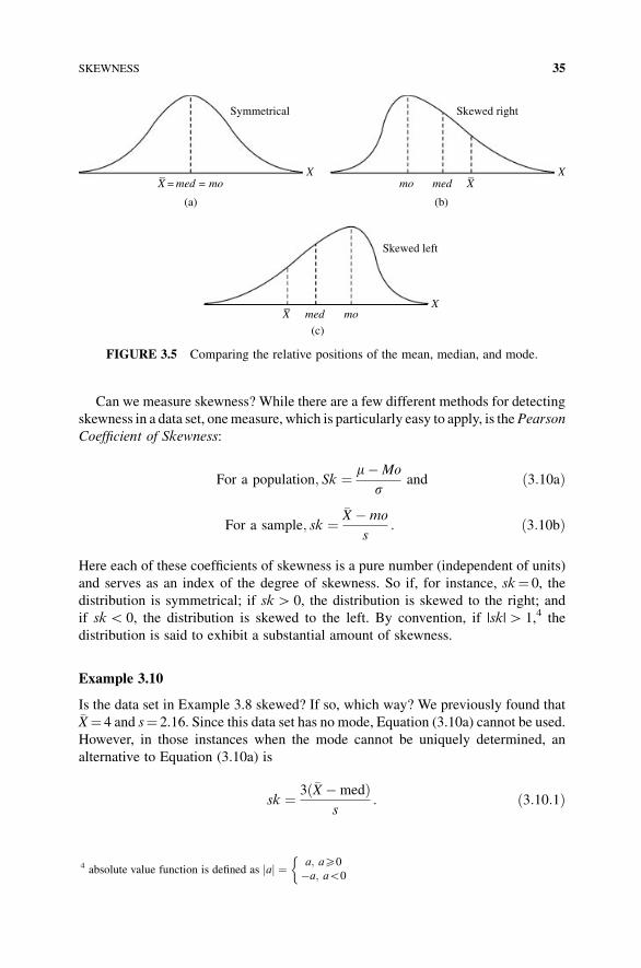
Can we measure skewness? While there are a few different methods for detecting
skewness in a data set, onemeasure, which is particularly easy to apply, is thePearson
Coefficient of Skewness:
For a population; Sk ¼ m�Mo
sand ð3:10aÞ
For a sample; sk ¼�X �mo
s: ð3:10bÞ
Here each of these coefficients of skewness is a pure number (independent of units)
and serves as an index of the degree of skewness. So if, for instance, sk¼ 0, the
distribution is symmetrical; if skH 0, the distribution is skewed to the right; and
if skG 0, the distribution is skewed to the left. By convention, if |sk|H 1,4 the
distribution is said to exhibit a substantial amount of skewness.
Example 3.10
Is the data set in Example 3.8 skewed? If so, which way? We previously found that�X¼ 4 and s¼ 2.16. Since this data set has no mode, Equation (3.10a) cannot be used.
However, in those instances when the mode cannot be uniquely determined, an
alternative to Equation (3.10a) is
sk ¼ 3ð�X �medÞs
: ð3:10:1Þ
(a) (b)
(c)
Symmetrical
Skewed left
Skewed right
X
XXXmedmo= med = mo –X–
X med mo–
FIGURE 3.5 Comparing the relative positions of the mean, median, and mode.
4 absolute value function is defined as aj j ¼ a; aX0
�a; aG0
�
SKEWNESS 35
Since the median for the variable X is med¼ 3.5, we can readily find that
sk ¼ 3ð4� 3:5Þ2:16
¼ 0:69:
Hence this data set is moderately skewed to the right.
Another option is to use as our measure of skewness the average of the cubed Z-scores
(called standard skewness) or
k3 ¼ Sni¼1Z
3i
n� 1¼ 1
S3Sni¼1ðXi � �XÞ3
n� 1: ð3:11Þ
When k3�0, the data set is taken to be symmetrical; for k3H 0, the data set is skewed
right; and for k3G 0, the data set is skewed left. If k3j jH0:5, the data set is said to
display a substantial amount of skewness. For instance, given the Example 3.8 data
set, the reader can easily verify that SðXi � �XÞ3 ¼ 18; s3 ¼ 10:08; and thus
k3 ¼ 110:08
183
� � ¼ 0:5952:Hence, according to Equation (3.11), this data set is highly skewed to the right.
3.9 QUANTILES
In general, we can view quantiles as positional measures that divide the observations
on a variable X into a number of equal portions (given that the data values are in an
increasing sequence). We have already encountered the median of a data set; it is a
positional value that splits the data into two equal parts. Others are:
Quartiles: Split the data into four equal parts
Deciles: Split the data into 10 equal parts
Percentiles: Split the data into 100 equal parts
There are three computed quartiles that will divide the observations on a variableX
into four equal parts: Q1, Q2, and Q3. In this regard, 25% of all observations on X lie
below Q1; 50% of all observations on X lie below Q2 (¼median); and 75% of all
observations on X lie below Q3. Remember that quartiles are “positional values.”
Hence the following:
Q1 is located atnþ 1
4ð3:12aÞ
Q2 is located atnþ 1
2ð3:12bÞ
36 DESCRIPTIVE CHARACTERISTICS OF QUANTITATIVE DATA
Q3 is located at3 nþ 1ð Þ
4ð3:12cÞ
(provided, of course, that our data have been arranged in an increasing sequence).
Given Equation (3.12), we can easily calculate the interquartile range (IQR) as
IQR¼Q3�Q1—it is the range between the first and third quartiles and serves to
locate themiddle 50% of the observations on a variableX. Then the quartile deviation
is readily formed as
q:d: ¼ IQR=2 ¼ ðQ3 � Q1Þ=2 ð3:13Þand can be used as a measure of dispersion in the middle half of a distribution—a
device that is particularly useful when outliers are present.
There are nine computed deciles that divide all the observations on X into 10 equal
parts:D1,D2, . . . ,D9. Thus 10%of all observations onX are belowD1, 20%of all data
points for X lie below D2, and so on. Here too deciles are “positional values” so that:
Dj is located atjðnþ 1Þ
10; j ¼ 1; . . . ; 9: ð3:14Þ
For instance, once all the observations onX are arranged in an increasing sequence,D7
occupies the position ð7=10Þ(nþ 1).
Finally, 99 computed percentiles divide the observations onX into 100 equal parts:
P1, P2, . . . , P99. Here 1% of all observations on X lie below P1, 2% of the X values lie
below P2, and so on. Looking to the positions of these percentiles, we find that:
Pj is located atjðnþ 1Þ100
; j ¼ 1; . . . ; 99; ð3:15Þ
with, say, P40 found at ð40=100Þ(n þ 1).
It is important to note thatwe can actuallymove in the reverse direction and find the
percentile that corresponds to a particular value of X. That is, to determine the
percentile of the score X0, find
Percentile of X0 ¼ Number of data pointsGX0
n� 100; ð3:16Þ
provided, of course, that the observations on X are in an increasing sequence. The
value obtained in Equation (3.16) is rounded to the nearest integer.
Example 3.11
Given the following set of observations on X: 3, 8, 8, 6, 7, 9, 5, 10, 11, 20, 19, 15, 11,
16, find Q1, D2 and P30. Upon arranging these n¼ 14 Xi’s in increasing order,
3; 5; 6; 7; 8; 8; 9; 10; 11; 11; 15; 16; 19; 20;
QUANTILES 37
we can easily determine that:
a. FromEquation (3.12a),Q1 is located at the position ð14þ 1Þ=4 ¼ 15=4 ¼ 3:75,that is, Q1 is
3=4 of the distance between the third and fourth data points. Hence
Q1¼ 6.75.
b. Using Equation (3.14),D2 is located at the position ð2ð14þ 1ÞÞ=10 ¼ 3 orD2 is
located at the third observation. Hence D2¼ 6.
c. From Equation (3.15), P30 is located at the position ð30ð14þ 1ÞÞ=100 ¼ 4:50:Thus P30 lies half the distance between the fourth and fifth data points. Thus
P30¼ 7.5.
Additionally, what is the percentile associated withX0 ¼ 15? From Equation (3.16),
Percentile of 15 ¼ 10
14� 100 ¼ 71:42:
Thus,X0 ¼ 15 locates the 71st percentile of theX values, that is, approximately 71%of
all observations on X lie below 15.
3.10 KURTOSIS
Theconceptofkurtosis refers tohowflator rounded thepeakofadistributionhappens to
be.While there are a variety of ways tomeasure the degree of kurtosis in a data set, one
approach,which is quite straightforward to apply, is the so-called coefficient of kurtosis:
k ¼ q:d:
P90 � P10
; ð3:17Þ
where the quartile deviation (q.d.) is determined from Equation (3.13). The benchmark
or point of reference for determining the degree of kurtosis for a data set is the normal
distribution (it is continuous, bell-shaped, and symmetrical). In this regard:
a. For a normal curve, k� 0.263.
b. For a flat curve, k� 0.
c. For a sharply peaked curve, k� 0.5.
Typically k is computed when one has a fairly large data set.
An alternative to Equation (3.17) is to calculate standard kurtosis as the average of
the Z-scores raised to the fourth power or
k4 ¼ Sni¼1Z
4i
n� 1¼ 1
s4Sni¼1ðXi � �XÞ4
n� 1: ð3:18Þ
For a normal distribution (again used as our benchmark), k4¼ 3. Then our estimate
of the degree of kurtosis is k4� 3 (called the excess). So if k4� 3H 0 (positive
kurtosis), the data set has a peak that is sharper than that of a normal distribution;
38 DESCRIPTIVE CHARACTERISTICS OF QUANTITATIVE DATA
and if k3� 3G 0 (negative kurtosis), the data set has a peak that is flatter than that
of a normal distribution. In this latter instance, the distribution might have
elongated tails, thus indicating the presence of outliers. For instance, again using
the Example 3.8 data set, it can be shown that SðXi � �XÞ4 ¼ 98, s4¼ 21.76, and
thus
k4 � 3 ¼ 1
21:76
98
3
� �� 3 ¼ �1:4988:
Hence this data set exhibits considerable uniformity—its peak ismuch flatter than that
of a normal distribution.
3.11 DETECTION OF OUTLIERS
Wenoted above that ameasure of central location such as themean is affected by each
observation in a data set and thus by extreme values. Extreme values may or may not
be outliers (atypical or unusually small or large data values). For instance, given the
data setX: 1, 3, 6, 7, 8, 10, it is obvious that 1 and 10 are extremevalues for this data set,
but they are not outliers. If, instead, we had X: 1, 3, 6, 7, 8, 42, then, clearly, 42 is an
extreme value that would also qualify as an outlier.
There are two ways to check a data set for outliers:
1. We can apply the empirical rule—for a data set that is normally distributed (or
approximately so, but certainly symmetrical), we can use Z-scores to identify
outliers: an observationXi is deemed an outlier if it isZ-scoreZi lies below –2.24
or above 2.24.Here� 2.24 are the cut-off points or fences that leave uswith only
2.5% of the data in each tail of the distribution. Both of these cases can be
subsumed under the inequality
jXi � �Xjs
H2:24: ð3:19Þ
While Equation (3.19) is commonly utilized to detect outliers, its usage ignores
a rather acute problem—the values of both �X and s are themselves affected by
outliers. Why should we use a device for detecting outliers that itself is
impacted by outliers? Since the median is not affected by outliers, let us
modify Equation (3.19) to obtain the following:
jXi �medjmad=0:6745
H2:24; ð3:19:1Þ
wheremad denotes the sample median absolute deviation that is determined as
the median of the absolute deviations from the median.
DETECTION OF OUTLIERS 39
That is, to find mad, first determine the set of absolute deviations from the
median or
X1 �medj j; X2 �medj j; . . . ; Xn �medj j
and then find their median or middle value.
Example 3.12
Suppose that from a normal population we randomly obtain the set of n¼ 10 sample
values:
0; 1; 1; 3; 4; 6; 8; 10; 11; 50:
Then med¼ 5 and
0� 5j j ¼ 5; 1� 5j j ¼ 4; 1� 5j j ¼ 4; 3� 5j j ¼ 2; 4� 5j j ¼ 1; 6� 5j j ¼ 1;
8� 5j j ¼ 3; 10� 5j j ¼ 5; 11� 5j j ¼ 6; 50� 5j j ¼ 45:
Arranging these absolute deviations from the median in an increasing sequence
yields
1; 1; 2; 3; 4; 4; 5; 5; 6; 45:
Then mad¼ 4 and, from Equation (3.19.1)
j50� 5j4=0:6745
¼ 7:58H2:24:
Thus only X¼ 50 can be considered to be an outlier.
2. We can employ quartiles—given the IQR¼Q3 – Q1, the fences are:
ðLowerÞ l ¼ Q1 � 1:5 IQR;
ðUpperÞ u ¼ Q3 þ 1:5 IQR:ð3:20Þ
So if a value ofX is less than the lower fence l or greater than the upper fence u, it
is considered to be an outlier.
Example 3.13
Given the n¼ 14 values of X appearing in Example 3.11, use the fences given by
Equation (3.20) to determine if this data set exhibits any outliers.We previously found
thatQ1¼ 6.75. SinceQ3 is located at the position3ð14þ1Þ
4¼ 11:25 (it is a quarter of the
40 DESCRIPTIVE CHARACTERISTICS OF QUANTITATIVE DATA
distance between the 11th and 12th data points), we find Q3¼ 15.25. Then IQR¼Q3�Q1¼ 8.50 and
l ¼ 6:75� 1:5 8:50ð Þ ¼ �6:0;
u ¼ 15:25þ 1:5 8:50ð Þ ¼ 28:0:
Since none of theXi’s is less than�6 or greater than 28, this data set does not have any
outliers.
Amodification of Equation (3.20) that employs departures from themedian is:Xi is an
outlier if
XiGmed� h IQR
or if
XiHmedþ h IQR;ð3:20:1Þ
where
h ¼ 17:63n� 23:64
7:74n� 3:71:
What if outliers are detected for somedata set?How should they be handled? Since the
mean, for example, is affected by the presence of outliers, one could possibly discard
any of the offending outlying values. However, if these data points are considered
important or essential to a study, then discarding them would obviously not be
appropriate. A useful alternative is to compute an a-trimmed mean, 0G aG 0.5, and
use it in place of �X. That is, for the set of n data points arranged in an increasing
sequence, the a�trimmed mean is determined by deleting the an smallest observa-
tions and the an largest observations, and then taking the arithmetic mean of the
remaining data points. For instance, if n¼ 30 and a¼ 0.10, then we would delete the
an¼ 3 smallest and largest values of X, and then compute the simple average of
the remaining 24 data values.
3.12 SO WHAT DO WE DO WITH ALL THIS STUFF?
How are the various descriptive measures developed in this chapter to be used in
analyzing a data set? To answer this question, we need only remember that the
characteristics of interest of a data set are shape, central location (“center” for short),
and dispersion (“spread” for short). In this regard:
1. If a distribution is symmetric (or nearly so)with no outliers, then �X and s provide
us with legitimate descriptions of center and spread, respectively. (This is so
because the values of �X and s are sensitive to both inordinately large or small
extremevalues of a variableX. And if the distribution lacks symmetry, no single
number can adequately describe spread since the two sides of a highly skewed
distribution have different spreads.)
SO WHAT DO WE DO WITH ALL THIS STUFF? 41
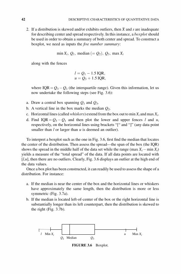
2. If a distribution is skewed and/or exhibits outliers, then �X and s are inadequate
for describing center and spread respectively. In this instance, a boxplot should
be used in order to obtain a summary of both center and spread. To construct a
boxplot, we need as inputs the five number summary:
min Xi; Q1; median ¼ Q2ð Þ; Q3; max Xi
along with the fences
l ¼ Q1 � 1:5 IQR;u ¼ Q3 þ 1:5 IQR;
where IQR¼Q3�Q1 (the interquartile range). Given this information, let us
now undertake the following steps (see Fig. 3.6):
a. Draw a central box spanning Q1 and Q3.
b. A vertical line in the box marks the median Q2.
c. Horizontal lines (calledwhiskers) extend from the box out tominXi andmaxXi.
d. Find IQR¼Q3�Q1 and then plot the lower and upper fences l and u,
respectively, on the horizontal lines using brackets “[“ and “]” (any data point
smaller than l or larger than u is deemed an outlier).
To interpret a boxplot such as the one in Fig. 3.6, first find the median that locates
the center of the distribution. Then assess the spread—the span of the box (the IQR)
shows the spread in the middle half of the data set while the range (max Xi�min Xi)
yields a measure of the “total spread” of the data. If all data points are located with
[l,u], then there are no outliers. Clearly, Fig. 3.6 displays an outlier at the high end of
the data values.
Once a box plot has been constructed, it can readily be used to assess the shape of a
distribution. For instance:
a. If the median is near the center of the box and the horizontal lines or whiskers
have approximately the same length, then the distribution is more or less
symmetric (Fig. 3.7a).
b. If the median is located left-of-center of the box or the right horizontal line is
substantially longer than its left counterpart, then the distribution is skewed to
the right (Fig. 3.7b).
[ ]l Min Xi u Max Xi
Q1 Median Q3
FIGURE 3.6 Boxplot.
42 DESCRIPTIVE CHARACTERISTICS OF QUANTITATIVE DATA
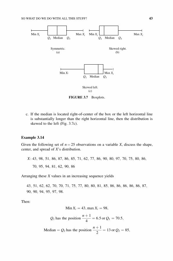
c. If the median is located right-of-center of the box or the left horizontal line
is substantially longer than the right horizontal line, then the distribution is
skewed to the left (Fig. 3.7c).
Example 3.14
Given the following set of n¼ 25 observations on a variable X, discuss the shape,
center, and spread of X’s distribution.
X : 43; 98; 51; 86; 87; 86; 85; 71; 62; 77; 86; 90; 80; 97; 70; 75; 80; 86;
70; 95; 94; 81; 62; 90; 86
Arranging these X values in an increasing sequence yields
43; 51; 62; 62; 70; 70; 71; 75; 77; 80; 80; 81; 85; 86; 86; 86; 86; 86; 87;
90; 90; 94; 95; 97; 98:
Then:
Min Xi ¼ 43;max Xi ¼ 98;
Q1 has the positionnþ 1
4¼ 6:5 orQ1 ¼ 70:5;
Median ¼ Q2 has the positionnþ 1
2¼ 13 orQ2 ¼ 85;
| | Min Xi Max Xi
Q1 Median Q3
Symmetric.(a)
| | Min Xi Max Xi
Q1 Median Q3
Skewed right.(b)
| | Min Xi Max Xi
Q1 Median Q3
Skewed left.(c)
FIGURE 3.7 Boxplots.
SO WHAT DO WE DO WITH ALL THIS STUFF? 43
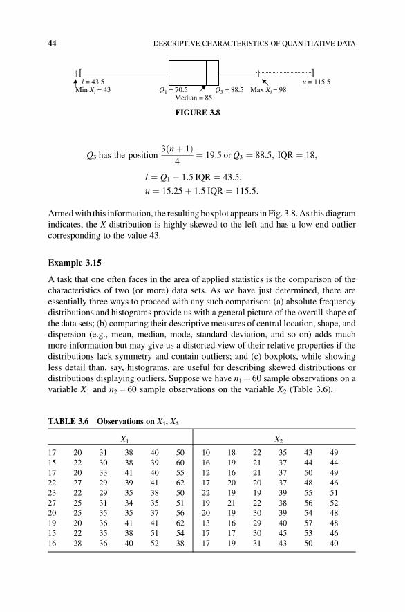
Q3 has the position3 nþ 1ð Þ
4¼ 19:5 orQ3 ¼ 88:5; IQR ¼ 18;
l ¼ Q1 � 1:5 IQR ¼ 43:5;
u ¼ 15:25þ 1:5 IQR ¼ 115:5:
Armedwith this information, the resulting boxplot appears in Fig. 3.8.As this diagram
indicates, the X distribution is highly skewed to the left and has a low-end outlier
corresponding to the value 43.
Example 3.15
A task that one often faces in the area of applied statistics is the comparison of the
characteristics of two (or more) data sets. As we have just determined, there are
essentially three ways to proceed with any such comparison: (a) absolute frequency
distributions and histograms provide us with a general picture of the overall shape of
the data sets; (b) comparing their descriptive measures of central location, shape, and
dispersion (e.g., mean, median, mode, standard deviation, and so on) adds much
more information but may give us a distorted view of their relative properties if the
distributions lack symmetry and contain outliers; and (c) boxplots, while showing
less detail than, say, histograms, are useful for describing skewed distributions or
distributions displaying outliers. Suppose we have n1¼ 60 sample observations on a
variable X1 and n2¼ 60 sample observations on the variable X2 (Table 3.6).
| [ | ]l = 43.5 u = 115.5
Min Xi = 43 Q1 = 70.5 Q3 = 88.5 Max Xi = 98Median = 85
FIGURE 3.8
TABLE 3.6 Observations on X1, X2
X1 X2
17 20 31 38 40 50 10 18 22 35 43 49
15 22 30 38 39 60 16 19 21 37 44 44
17 20 33 41 40 55 12 16 21 37 50 49
22 27 29 39 41 62 17 20 20 37 48 46
23 22 29 35 38 50 22 19 19 39 55 51
27 25 31 34 35 51 19 21 22 38 56 52
20 25 35 35 37 56 20 19 30 39 54 48
19 20 36 41 41 62 13 16 29 40 57 48
15 22 35 38 51 54 17 17 30 45 53 46
16 28 36 40 52 38 17 19 31 43 50 40
44 DESCRIPTIVE CHARACTERISTICS OF QUANTITATIVE DATA
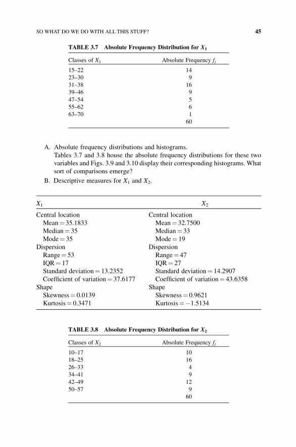
A. Absolute frequency distributions and histograms.
Tables 3.7 and 3.8 house the absolute frequency distributions for these two
variables and Figs. 3.9 and 3.10 display their corresponding histograms. What
sort of comparisons emerge?
B. Descriptive measures for X1 and X2.
X1 X2
Central location Central location
Mean¼ 35.1833 Mean¼ 32.7500
Median¼ 35 Median¼ 33
Mode¼ 35 Mode¼ 19
Dispersion Dispersion
Range¼ 53 Range¼ 47
IQR¼ 17 IQR¼ 27
Standard deviation¼ 13.2352 Standard deviation¼ 14.2907
Coefficient of variation¼ 37.6177 Coefficient of variation¼ 43.6358
Shape Shape
Skewness¼ 0.0139 Skewness¼ 0.9621
Kurtosis¼ 0.3471 Kurtosis¼�1.5134
TABLE 3.8 Absolute Frequency Distribution for X2
Classes of X2 Absolute Frequency fj
10–17 10
18–25 16
26–33 4
34–41 9
42–49 12
50–57 9
60
TABLE 3.7 Absolute Frequency Distribution for X1
Classes of X1 Absolute Frequency fj
15–22 14
23–30 9
31–38 16
39–46 9
47–54 5
55–62 6
63–70 1
60
SO WHAT DO WE DO WITH ALL THIS STUFF? 45
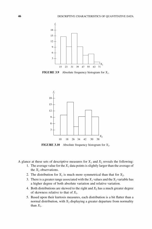
A glance at these sets of descriptive measures for X1 and X2 reveals the following:
1. The average value for the X1 data points is slightly larger than the average of
the X2 observations.
2. The distribution for X1 is much more symmetrical than that for X2.
3. There is a greater range associated with theX1 values and theX2 variable has
a higher degree of both absolute variation and relative variation.
4. Both distributions are skewed to the right and X2 has a much greater degree
of skewness relative to that of X1.
5. Based upon their kurtosis measures, each distribution is a bit flatter than a
normal distribution, with X2 displaying a greater departure from normality
than X1.
fj
18 —
15 —
12 —
9 —
6 —
3 —
X210 18 26 34 42 50 58
FIGURE 3.10 Absolute frequency histogram for X2.
fj
18 —
15 —
12 —
9 —
6 —
3 —
X115 23 31 39 47 55 63 71
FIGURE 3.9 Absolute frequency histogram for X1.
46 DESCRIPTIVE CHARACTERISTICS OF QUANTITATIVE DATA
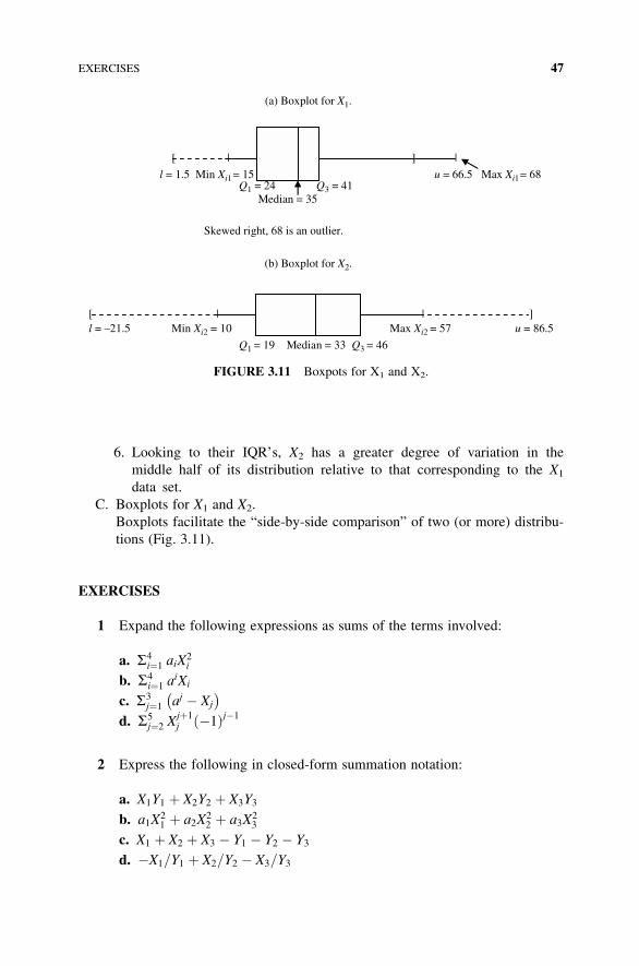
6. Looking to their IQR’s, X2 has a greater degree of variation in the
middle half of its distribution relative to that corresponding to the X1
data set.
C. Boxplots for X1 and X2.
Boxplots facilitate the “side-by-side comparison” of two (or more) distribu-
tions (Fig. 3.11).
EXERCISES
1 Expand the following expressions as sums of the terms involved:
a. S4i¼1 aiX
2i
b. S4i¼1 a
iXi
c. S3j¼1 aj � Xj
� �
d. S5j¼2 X
jþ1j �1ð Þj�1
2 Express the following in closed-form summation notation:
a. X1Y1 þ X2Y2 þ X3Y3
b. a1X21 þ a2X
22 þ a3X
23
c. X1 þ X2 þ X3 � Y1 � Y2 � Y3
d. �X1=Y1 þ X2=Y2 � X3=Y3
(a) Boxplot for X1.
[ | ] |
l = 1.5 Min Xi1 = 15 u = 66.5 Max Xi1= 68 Q1 = 24 Q3 = 41
Median = 35
Skewed right, 68 is an outlier.
(b) Boxplot for X2.
[ | | ] l = –21.5 Min Xi2 = 10 Max Xi2 = 57 u = 86.5
Q1 = 19 Median = 33 Q3 = 46
FIGURE 3.11 Boxpots for X1 and X2.
EXERCISES 47
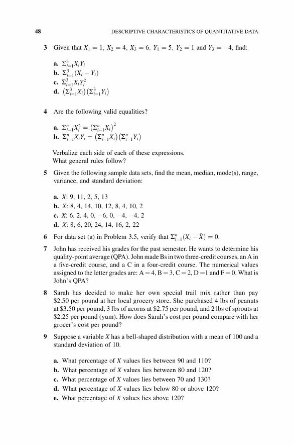
3 Given that X1 ¼ 1; X2 ¼ 4; X3 ¼ 6; Y1 ¼ 5; Y2 ¼ 1 and Y3 ¼ �4, find:
a. S3i¼1XiYi
b. S3i¼1 Xi � Yið Þ
c. S3i¼1XiY
2i
d. S3i¼1Xi
� �S3i¼1Yi
� �
4 Are the following valid equalities?
a. Sni¼1X
2i ¼ Sn
i¼1Xi
� �2
b. Sni¼1XiYi ¼ Sn
i¼1Xi
� �Sni¼1Yi
� �
Verbalize each side of each of these expressions.
What general rules follow?
5 Given the following sample data sets, find the mean, median, mode(s), range,
variance, and standard deviation:
a. X: 9, 11, 2, 5, 13
b. X: 8, 4, 14, 10, 12, 8, 4, 10, 2
c. X: 6, 2, 4, 0, �6, 0, �4, �4, 2
d. X: 8, 6, 20, 24, 14, 16, 2, 22
6 For data set (a) in Problem 3.5, verify that Sni¼1 Xi � �Xð Þ ¼ 0.
7 John has received his grades for the past semester. He wants to determine his
quality-point average (QPA). JohnmadeBs in two three-credit courses, anA in
a five-credit course, and a C in a four-credit course. The numerical values
assigned to the letter grades are: A¼ 4, B¼ 3, C¼ 2, D¼1 and F¼ 0. What is
John’s QPA?
8 Sarah has decided to make her own special trail mix rather than pay
$2.50 per pound at her local grocery store. She purchased 4 lbs of peanuts
at $3.50 per pound, 3 lbs of acorns at $2.75 per pound, and 2 lbs of sprouts at
$2.25 per pound (yum). How does Sarah’s cost per pound compare with her
grocer’s cost per pound?
9 Suppose a variable X has a bell-shaped distribution with a mean of 100 and a
standard deviation of 10.
a. What percentage of X values lies between 90 and 110?
b. What percentage of X values lies between 80 and 120?
c. What percentage of X values lies between 70 and 130?
d. What percentage of X values lies below 80 or above 120?
e. What percentage of X values lies above 120?
48 DESCRIPTIVE CHARACTERISTICS OF QUANTITATIVE DATA
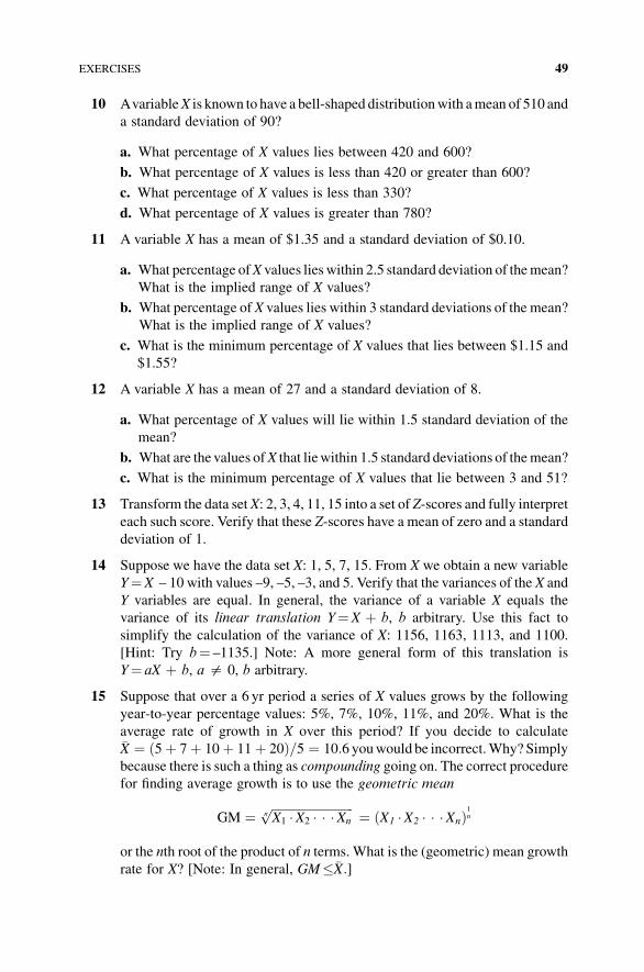
10 AvariableX is known to have a bell-shaped distributionwith amean of 510 and
a standard deviation of 90?
a. What percentage of X values lies between 420 and 600?
b. What percentage of X values is less than 420 or greater than 600?
c. What percentage of X values is less than 330?
d. What percentage of X values is greater than 780?
11 A variable X has a mean of $1.35 and a standard deviation of $0.10.
a. What percentage ofX values lies within 2.5 standard deviation of themean?
What is the implied range of X values?
b. What percentage of X values lies within 3 standard deviations of the mean?
What is the implied range of X values?
c. What is the minimum percentage of X values that lies between $1.15 and
$1.55?
12 A variable X has a mean of 27 and a standard deviation of 8.
a. What percentage of X values will lie within 1.5 standard deviation of the
mean?
b. What are the values ofX that liewithin 1.5 standard deviations of themean?
c. What is the minimum percentage of X values that lie between 3 and 51?
13 Transform the data setX: 2, 3, 4, 11, 15 into a set of Z-scores and fully interpret
each such score. Verify that these Z-scores have a mean of zero and a standard
deviation of 1.
14 Suppose we have the data set X: 1, 5, 7, 15. From X we obtain a new variable
Y¼X – 10 with values –9, –5, –3, and 5. Verify that the variances of the X and
Y variables are equal. In general, the variance of a variable X equals the
variance of its linear translation Y¼X þ b, b arbitrary. Use this fact to
simplify the calculation of the variance of X: 1156, 1163, 1113, and 1100.
[Hint: Try b¼ –1135.] Note: A more general form of this translation is
Y¼ aX þ b, a $ 0, b arbitrary.
15 Suppose that over a 6 yr period a series of X values grows by the following
year-to-year percentage values: 5%, 7%, 10%, 11%, and 20%. What is the
average rate of growth in X over this period? If you decide to calculate�X ¼ 5þ 7þ 10þ 11þ 20ð Þ=5 ¼ 10:6 youwould be incorrect.Why? Simply
because there is such a thing as compounding going on. The correct procedure
for finding average growth is to use the geometric mean
GM ¼ ffiffiffiffiffiffiffiffiffiffiffiffiffiffiffiffiffiffiffiffiffiffiffiffiffiffiffiX1 �X2 � � �Xn
np ¼ X1 �X2 � � �Xnð Þ1n
or the nth root of the product of n terms. What is the (geometric) mean growth
rate for X? [Note: In general, GM��X:]
EXERCISES 49
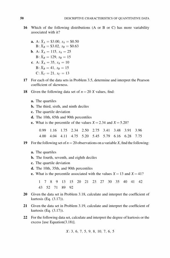
16 Which of the following distributions (A or B or C) has more variability
associated with it?
a. A : �XA ¼ $3:00; sA ¼ $0:50B: �XB ¼ $3:02; sB ¼ $0:63
b: A: �XA ¼ 115; sA ¼ 25
B: �XB ¼ 129; sB ¼ 15
c: A : �XA ¼ 35; sA ¼ 10
B: �XB ¼ 41; sB ¼ 15
C: �XC ¼ 21; sC ¼ 13
17 For each of the data sets in Problem 3.5, determine and interpret the Pearson
coefficient of skewness.
18 Given the following data set of n¼ 20 X values, find:
a. The quartiles
b. The third, sixth, and ninth deciles
c. The quartile deviation
d. The 10th, 65th and 90th percentiles
e. What is the percentile of the values X¼ 2.34 and X¼ 5.20?
0:99 1:16 1:75 2:34 2:50 2:75 3:41 3:48 3:91 3:96
4:00 4:04 4:11 4:75 5:20 5:45 5:79 6:16 6:28 7:75
19 For the following set of n¼ 20 observations on a variableX, find the following:
a. The quartiles
b. The fourth, seventh, and eighth deciles
c. The quartile deviation
d. The 10th, 35th, and 90th percentiles
e. What is the percentile associated with the values X¼ 13 and X¼ 41?
1 7 8 9 13 15 20 21 23 27 30 35 40 41 42
43 52 71 89 92
20 Given the data set in Problem 3.18, calculate and interpret the coefficient of
kurtosis (Eq. (3.17)).
21 Given the data set in Problem 3.19, calculate and interpret the coefficient of
kurtosis (Eq. (3.17)).
22 For the following data set, calculate and interpret the degree of kurtosis or the
excess [use Equation(3.18)].
X : 3; 6; 7; 5; 9; 8; 10; 7; 6; 5
50 DESCRIPTIVE CHARACTERISTICS OF QUANTITATIVE DATA
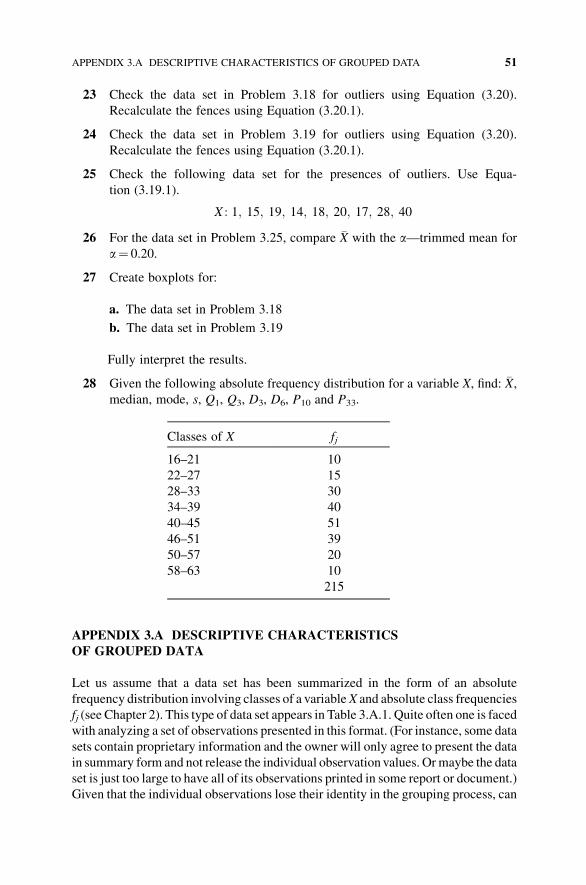
23 Check the data set in Problem 3.18 for outliers using Equation (3.20).
Recalculate the fences using Equation (3.20.1).
24 Check the data set in Problem 3.19 for outliers using Equation (3.20).
Recalculate the fences using Equation (3.20.1).
25 Check the following data set for the presences of outliers. Use Equa-
tion (3.19.1).
X : 1; 15; 19; 14; 18; 20; 17; 28; 40
26 For the data set in Problem 3.25, compare �X with the a—trimmed mean for
a¼ 0.20.
27 Create boxplots for:
a. The data set in Problem 3.18
b. The data set in Problem 3.19
Fully interpret the results.
28 Given the following absolute frequency distribution for a variable X, find: �X,median, mode, s, Q1, Q3, D3, D6, P10 and P33.
Classes of X fj
16–21 10
22–27 15
28–33 30
34–39 40
40–45 51
46–51 39
50–57 20
58–63 10
215
APPENDIX 3.A DESCRIPTIVE CHARACTERISTICSOF GROUPED DATA
Let us assume that a data set has been summarized in the form of an absolute
frequency distribution involving classes of a variableX and absolute class frequencies
fj (see Chapter 2). This type of data set appears in Table 3.A.1. Quite often one is faced
with analyzing a set of observations presented in this format. (For instance, some data
sets contain proprietary information and the owner will only agree to present the data
in summary form and not release the individual observation values. Ormaybe the data
set is just too large to have all of its observations printed in some report or document.)
Given that the individual observations lose their identity in the grouping process, can
APPENDIX 3.A DESCRIPTIVE CHARACTERISTICS OF GROUPED DATA 51
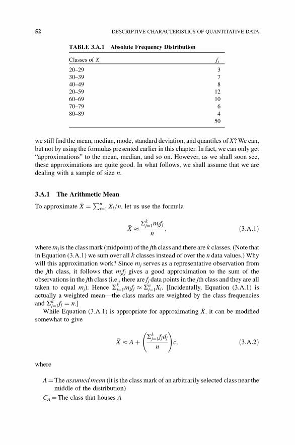
we still find the mean, median, mode, standard deviation, and quantiles of X?We can,
but not by using the formulas presented earlier in this chapter. In fact, we can only get
“approximations” to the mean, median, and so on. However, as we shall soon see,
these approximations are quite good. In what follows, we shall assume that we are
dealing with a sample of size n.
3.A.1 The Arithmetic Mean
To approximate �X ¼Pni¼1 Xi=n, let us use the formula
�X � Skj¼1mjfj
n; ð3:A:1Þ
wheremj is the classmark (midpoint) of the jth class and there are k classes. (Note that
in Equation (3.A.1) we sum over all k classes instead of over the n data values.) Why
will this approximation work? Since mj serves as a representative observation from
the jth class, it follows that mjfj gives a good approximation to the sum of the
observations in the jth class (i.e., there are fj data points in the jth class and they are all
taken to equal mj). Hence Skj¼1mjfj � Sn
i¼1Xi. [Incidentally, Equation (3.A.1) is
actually a weighted mean—the class marks are weighted by the class frequencies
and Skj¼1fj ¼ n.]
While Equation (3.A.1) is appropriate for approximating �X, it can be modified
somewhat to give
�X � Aþ Skj¼1fjdj
n
!c; ð3:A:2Þ
where
A¼The assumedmean (it is the class mark of an arbitrarily selected class near the
middle of the distribution)
CA¼The class that houses A
TABLE 3.A.1 Absolute Frequency Distribution
Classes of X fj
20–29 3
30–39 7
40–49 8
20–59 12
60–69 10
70–79 6
80–89 4
50
52 DESCRIPTIVE CHARACTERISTICS OF QUANTITATIVE DATA
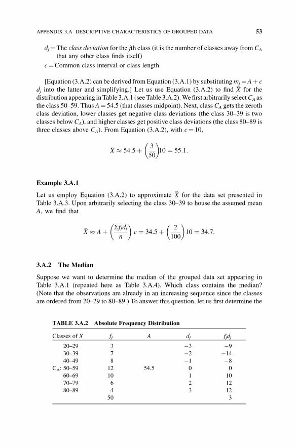
dj¼The class deviation for the jth class (it is the number of classes away from CA
that any other class finds itself)
c¼Common class interval or class length
[Equation (3.A.2) can be derived from Equation (3.A.1) by substitutingmj¼Aþ c
dj into the latter and simplifying.] Let us use Equation (3.A.2) to find �X for the
distribution appearing in Table 3.A.1 (see Table 3.A.2).Wefirst arbitrarily selectCA as
the class 50–59. Thus A¼ 54.5 (that classes midpoint). Next, class CA gets the zeroth
class deviation, lower classes get negative class deviations (the class 30–39 is two
classes below CA), and higher classes get positive class deviations (the class 80–89 is
three classes above CA). From Equation (3.A.2), with c¼ 10,
�X � 54:5þ 3
50
� �10 ¼ 55:1:
Example 3.A.1
Let us employ Equation (3.A.2) to approximate �X for the data set presented in
Table 3.A.3. Upon arbitrarily selecting the class 30–39 to house the assumed mean
A, we find that
�X � Aþ Sfjdjn
� �c ¼ 34:5þ 2
100
� �10 ¼ 34:7:
3.A.2 The Median
Suppose we want to determine the median of the grouped data set appearing in
Table 3.A.1 (repeated here as Table 3.A.4). Which class contains the median?
(Note that the observations are already in an increasing sequence since the classes
are ordered from 20–29 to 80–89.) To answer this question, let us first determine the
TABLE 3.A.2 Absolute Frequency Distribution
Classes of X fj A dj fjdj
20–29 3 �3 �9
30–39 7 �2 �14
40–49 8 �1 �8
CA: 50–59 12 54.5 0 0
60–69 10 1 10
70–79 6 2 12
80–89 4 3 12
50 3
APPENDIX 3.A DESCRIPTIVE CHARACTERISTICS OF GROUPED DATA 53
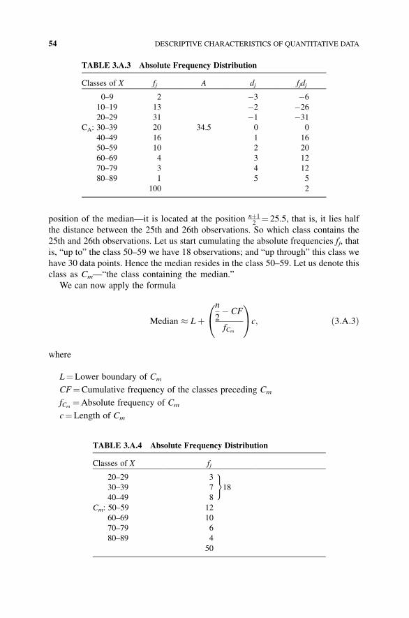
position of the median—it is located at the position nþ12¼ 25.5, that is, it lies half
the distance between the 25th and 26th observations. So which class contains the
25th and 26th observations. Let us start cumulating the absolute frequencies fj, that
is, “up to” the class 50–59 we have 18 observations; and “up through” this class we
have 30 data points. Hence the median resides in the class 50–59. Let us denote this
class as Cm—“the class containing the median.”
We can now apply the formula
Median � Lþn
2� CF
fCm
0@
1Ac; ð3:A:3Þ
where
L¼Lower boundary of Cm
CF¼Cumulative frequency of the classes preceding Cm
fCm¼Absolute frequency of Cm
c¼Length of Cm
TABLE 3.A.3 Absolute Frequency Distribution
Classes of X fj A dj fjdj
0–9 2 �3 �6
10–19 13 �2 �26
20–29 31 �1 �31
CA: 30–39 20 34.5 0 0
40–49 16 1 16
50–59 10 2 20
60–69 4 3 12
70–79 3 4 12
80–89 1 5 5
100 2
TABLE 3.A.4 Absolute Frequency Distribution
Classes of X fj
20–29 3
30–39 7
�18
40–49 8
Cm: 50–59 12
60–69 10
70–79 6
80–89 4
50
54 DESCRIPTIVE CHARACTERISTICS OF QUANTITATIVE DATA
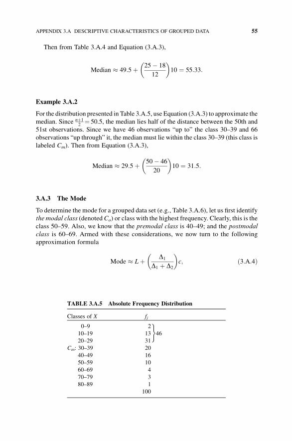
Then from Table 3.A.4 and Equation (3.A.3),
Median � 49:5þ 25� 18
12
� �10 ¼ 55:33:
Example 3.A.2
For the distribution presented in Table 3.A.5, use Equation (3.A.3) to approximate the
median. Since nþ12¼ 50.5, the median lies half of the distance between the 50th and
51st observations. Since we have 46 observations “up to” the class 30–39 and 66
observations “up through” it, the median must lie within the class 30–39 (this class is
labeled Cm). Then from Equation (3.A.3),
Median � 29:5þ 50� 46
20
� �10 ¼ 31:5:
3.A.3 The Mode
To determine the mode for a grouped data set (e.g., Table 3.A.6), let us first identify
the modal class (denoted Co) or class with the highest frequency. Clearly, this is the
class 50–59. Also, we know that the premodal class is 40–49; and the postmodal
class is 60–69. Armed with these considerations, we now turn to the following
approximation formula
Mode � Lþ D1
D1 þ D2
� �c; ð3:A:4Þ
TABLE 3.A.5 Absolute Frequency Distribution
Classes of X fj
0–9 2
10–19 13
�46
20–29 31
Cm: 30–39 20
40–49 16
50–59 10
60–69 4
70–79 3
80–89 1
100
APPENDIX 3.A DESCRIPTIVE CHARACTERISTICS OF GROUPED DATA 55
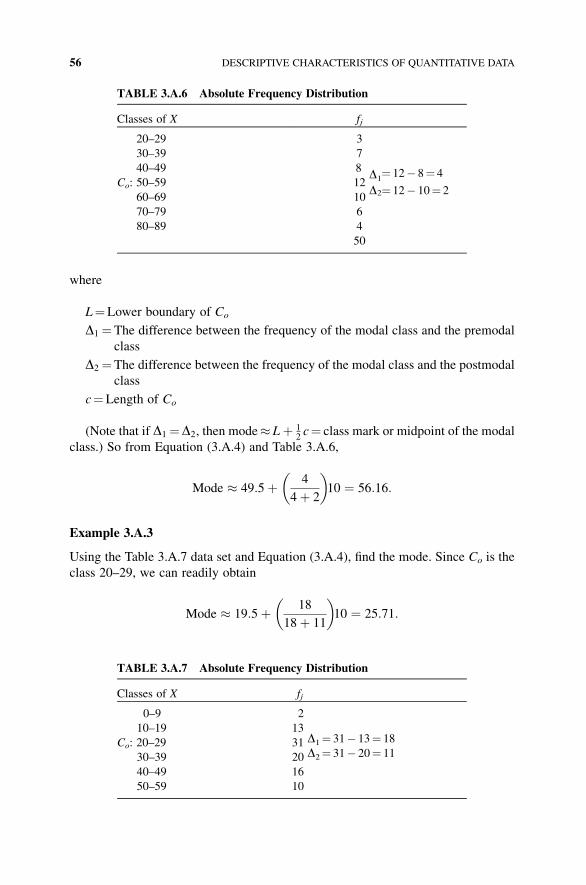
where
L¼Lower boundary of Co
D1 ¼The difference between the frequency of the modal class and the premodal
class
D2 ¼The difference between the frequency of the modal class and the postmodal
class
c¼Length of Co
(Note that if D1 ¼D2, then mode� Lþ 12c¼ class mark or midpoint of the modal
class.) So from Equation (3.A.4) and Table 3.A.6,
Mode � 49:5þ 4
4þ 2
� �10 ¼ 56:16:
Example 3.A.3
Using the Table 3.A.7 data set and Equation (3.A.4), find the mode. Since Co is the
class 20–29, we can readily obtain
Mode � 19:5þ 18
18þ 11
� �10 ¼ 25:71:
TABLE 3.A.6 Absolute Frequency Distribution
Classes of X fj
20–29 3
30–39 7
40–49 8 D1¼ 12� 8¼ 4
Co: 50–59 12
60–69 10D2¼ 12� 10¼ 2
70–79 6
80–89 4
50
TABLE 3.A.7 Absolute Frequency Distribution
Classes of X fj
0–9 2
10–19 13D1¼ 31� 13¼ 18Co: 20–29 31
30–39 20 D2¼ 31� 20¼ 11
40–49 16
50–59 10
56 DESCRIPTIVE CHARACTERISTICS OF QUANTITATIVE DATA
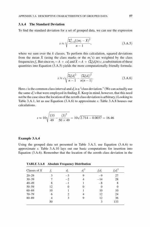
3.A.4 The Standard Deviation
To find the standard deviation for a set of grouped data, we can use the expression
s �ffiffiffiffiffiffiffiffiffiffiffiffiffiffiffiffiffiffiffiffiffiffiffiffiffiffiffiffiffiffiffiSkj¼1fjðmj � �XÞ2
n� 1
s
; ð3:A:5Þ
where we sum over the k classes. To perform this calculation, squared deviations
from the mean �X (using the class marks or the mj’s) are weighted by the class
frequencies fj. But sincemj¼A þ cdj and �X¼A þ (Sfjdj/n) c, a substitution of thesequantities into Equation (3.A.5) yields the more computationally friendly formula:
s � c
ffiffiffiffiffiffiffiffiffiffiffiffiffiffiffiffiffiffiffiffiffiffiffiffiffiffiffiffiffiffiffiffiffiffiffiSfjdj
2
n� 1� ðSfjdjÞ2nðn� 1Þ
s
: ð3:A:6Þ
Here c is the common class interval and dj is a “class deviation.” (We can actually use
the same dj’s that were employed in finding �X. Keep in mind, however, that this need
not be the case since the location of the zeroth class deviation is arbitrary.) Looking to
Table 3.A.1, let us use Equation (3.A.6) to approximate s. Table 3.A.8 houses our
calculations.
s � 10
ffiffiffiffiffiffiffiffiffiffiffiffiffiffiffiffiffiffiffiffiffiffiffiffiffiffiffiffiffi133
49� ð3Þ250� 49
s
¼ 10ffiffiffiffiffiffiffiffiffiffiffiffiffiffiffiffiffiffiffiffiffiffiffiffiffiffiffiffiffiffiffi2:714� 0:0037
p¼ 16:46
Example 3.A.4
Using the grouped data set presented in Table 3.A.3, use Equation (3.A.6) to
approximate s. Table 3.A.10 lays out our basic computations for insertion into
Equation (3.A.6). Remember that the location of the zeroth class deviation in the
TABLE 3.A.8 Absolute Frequency Distribution
Classes of X fj dj dj2 fjdj fjdj
2
20–29 3 �3 9 �9 27
30–39 7 �2 4 �14 28
40–49 8 �1 1 �8 8
50–59 12 0 0 0 0
60–69 10 1 1 10 10
70–79 6 2 4 12 24
80–89 4 3 9 12 36
50 3 133
APPENDIX 3.A DESCRIPTIVE CHARACTERISTICS OF GROUPED DATA 57
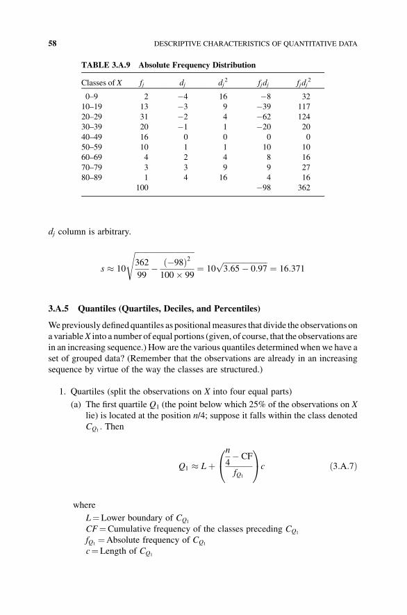
dj column is arbitrary.
s � 10
ffiffiffiffiffiffiffiffiffiffiffiffiffiffiffiffiffiffiffiffiffiffiffiffiffiffiffiffiffiffiffi362
99� ð�98Þ2100� 99
s
¼ 10ffiffiffiffiffiffiffiffiffiffiffiffiffiffiffiffiffiffiffiffiffiffiffi3:65� 0:97
p¼ 16:371
3.A.5 Quantiles (Quartiles, Deciles, and Percentiles)
Wepreviously definedquantiles as positionalmeasures that divide the observations on
a variableX into a number of equal portions (given, of course, that the observations are
in an increasing sequence.) How are the various quantiles determined when we have a
set of grouped data? (Remember that the observations are already in an increasing
sequence by virtue of the way the classes are structured.)
1. Quartiles (split the observations on X into four equal parts)
(a) The first quartile Q1 (the point below which 25% of the observations on X
lie) is located at the position n/4; suppose it falls within the class denoted
CQ1: Then
Q1 � Lþn
4� CF
fQ1
0
@
1
Ac ð3:A:7Þ
where
L¼Lower boundary of CQ1
CF¼Cumulative frequency of the classes preceding CQ1
fQ1¼Absolute frequency of CQ1
c¼Length of CQ1
TABLE 3.A.9 Absolute Frequency Distribution
Classes of X fj dj dj2 fjdj fjdj
2
0–9 2 �4 16 �8 32
10–19 13 �3 9 �39 117
20–29 31 �2 4 �62 124
30–39 20 �1 1 �20 20
40–49 16 0 0 0 0
50–59 10 1 1 10 10
60–69 4 2 4 8 16
70–79 3 3 9 9 27
80–89 1 4 16 4 16
100 �98 362
58 DESCRIPTIVE CHARACTERISTICS OF QUANTITATIVE DATA
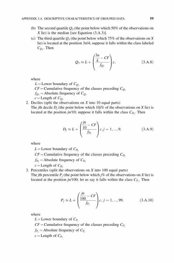
(b) The second quartileQ2 (the point below which 50% of the observations on
X lie) is the median [see Equation (3.A.3)].
(c) The third quartile Q3 (the point below which 75% of the observations on X
lie) is located at the position 3n/4; suppose it falls within the class labeled
CQ3. Then
Q3 � Lþ3n
4� CF
fQ3
0
B@
1
CAc; ð3:A:8Þ
where
L¼Lower boundary of CQ3
CF¼Cumulative frequency of the classes preceding CQ3
fQ3¼Absolute frequency of CQ3
c¼Length of CQ3
2. Deciles (split the observations on X into 10 equal parts)
The jth decile Dj (the point below which 10j% of the observations on X lie) is
located at the position jn/10; suppose it falls within the class CDj. Then
Dj � Lþjn
10� CF
fDj
0B@
1CAc; j ¼ 1; :::; 9; ð3:A:9Þ
where
L¼Lower boundary of CDj
CF¼Cumulative frequency of the classes preceding CDj
fDj¼Absolute frequency of CDj
c¼Length of CDj
3. Percentiles (split the observations on X into 100 equal parts)
The jth percentile Pj (the point below which j% of the observations on X lie) is
located at the position jn/100; let us say it falls within the class CPj. Then
Pj � Lþjn
100� CF
fPj
0B@
1CAc; j ¼ 1; :::; 99; ð3:A:10Þ
where
L¼Lower boundary of CPj
CF¼Cumulative frequency of the classes preceding CPj
fPj¼Absolute frequency of CPj
c¼Length of CPj
APPENDIX 3.A DESCRIPTIVE CHARACTERISTICS OF GROUPED DATA 59
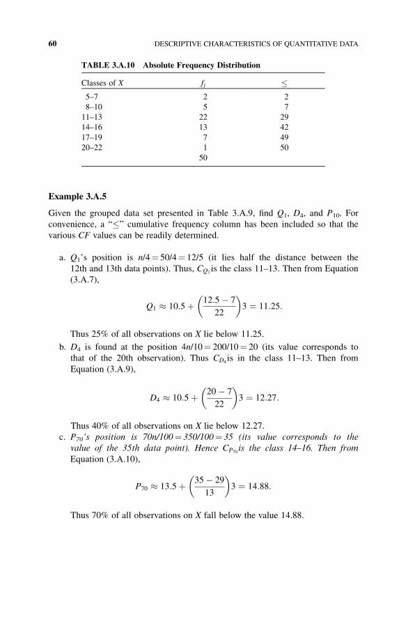
Example 3.A.5
Given the grouped data set presented in Table 3.A.9, find Q1, D4, and P10. For
convenience, a “�” cumulative frequency column has been included so that the
various CF values can be readily determined.
a. Q1’s position is n/4¼ 50/4¼ 12/5 (it lies half the distance between the
12th and 13th data points). Thus, CQ1is the class 11–13. Then from Equation
(3.A.7),
Q1 � 10:5þ 12:5� 7
22
� �3 ¼ 11:25:
Thus 25% of all observations on X lie below 11.25.
b. D4 is found at the position 4n/10¼ 200/10¼ 20 (its value corresponds to
that of the 20th observation). Thus CD4is in the class 11–13. Then from
Equation (3.A.9),
D4 � 10:5þ 20� 7
22
� �3 ¼ 12:27:
Thus 40% of all observations on X lie below 12.27.
c. P70’s position is 70n/100¼ 350/100¼ 35 (its value corresponds to the
value of the 35th data point). Hence CP70is the class 14–16. Then from
Equation (3.A.10),
P70 � 13:5þ 35� 29
13
� �3 ¼ 14:88:
Thus 70% of all observations on X fall below the value 14.88.
TABLE 3.A.10 Absolute Frequency Distribution
Classes of X fj �5–7 2 2
8–10 5 7
11–13 22 29
14–16 13 42
17–19 7 49
20–22 1 50
50
60 DESCRIPTIVE CHARACTERISTICS OF QUANTITATIVE DATA
4ESSENTIALS OF PROBABILITY
4.1 SET NOTATION
This section offers a brief review of set notation and concepts (readers familiar with
this material showed proceed to the next section). These (set) notions are important in
that they offer the reader a way of “thinking” or a way to “organize information”.
As we shall see shortly, only “events” have probabilities associated with them, and
these events are easily visualized/described and conveniently manipulated via set
operations.
Let us define a set as a collection or grouping of itemswithout regard to structure or
order—we have an amorphous group of items. Sets will be denoted using capital
letters (A, B,C, . . .). An element is a member of a set. Elements will be denoted using
small-case letters (a, b, c, . . .). A set is defined by listing its elements. If forming a list
is impractical or impossible, then we can define a set in terms of some key property
that the elements, and only the elements, of the set possess. For instance, the set of all
odd numbers can be defined as N ¼ fn nþ 1 is evengj . Here n is a representative
member of the set N and the vertical bar reads “such that.”
If an elementx is amember of setX, wewritex 2 X(element inclusion); ifx is not a
member ofX; then x =2 X(we negate the element inclusion symbol). If setA is a subset
ofB (a subset is a set within a set), wewriteA � B(set inclusion); ifA is not a subset of
B, then A 6�B (we negate the set inclusion symbol).1
Statistical Inference: A Short Course, First Edition. Michael J. Panik.� 2012 John Wiley & Sons, Inc. Published 2012 by John Wiley & Sons, Inc.
1 IfA � B; then eitherA � B (A is a proper subsetofB, meaning thatB is a larger set) orA¼B. Actually, set
equality is formally defined as follows: if A � B; and B � A; then A¼B.
61
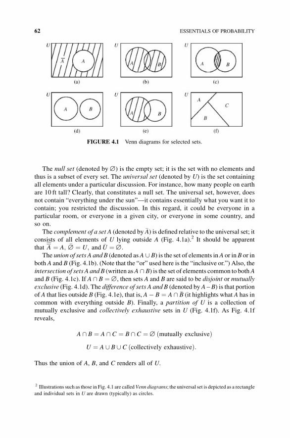
The null set (denoted by ˘) is the empty set; it is the set with no elements and
thus is a subset of every set. The universal set (denoted by U) is the set containing
all elements under a particular discussion. For instance, how many people on earth
are 10 ft tall? Clearly, that constitutes a null set. The universal set, however, does
not contain “everything under the sun”—it contains essentially what you want it to
contain; you restricted the discussion. In this regard, it could be everyone in a
particular room, or everyone in a given city, or everyone in some country, and
so on.
The complement of a set A (denoted by �A) is defined relative to the universal set; itconsists of all elements of U lying outside A (Fig. 4.1a).2 It should be apparent
that A ¼ A; � ¼ U; and �U ¼ ˘:The union of sets A and B (denoted as A [ B) is the set of elements inA or inB or in
both A and B (Fig. 4.1b). (Note that the “or” used here is the “inclusive or.”) Also, the
intersection of sets A and B (written asA \ B) is the set of elements common to bothA
and B (Fig. 4.1c). If A \ B ¼ ˘, then sets A and B are said to be disjoint or mutually
exclusive (Fig. 4.1d). The difference of sets A and B (denoted by A – B) is that portion
of A that lies outside B (Fig. 4.1e), that is, A� B ¼ A \ �B (it highlights what A has in
common with everything outside B). Finally, a partition of U is a collection of
mutually exclusive and collectively exhaustive sets in U (Fig. 4.1f). As Fig. 4.1f
reveals,
A \ B ¼ A \ C ¼ B \ C ¼ ˘ ðmutually exclusiveÞU ¼ A [ B [ C ðcollectively exhaustiveÞ:
Thus the union of A, B, and C renders all of U.
FIGURE 4.1 Venn diagrams for selected sets.
2 Illustrations such as those in Fig. 4.1 are calledVenn diagrams; the universal set is depicted as a rectangle
and individual sets in U are drawn (typically) as circles.
62 ESSENTIALS OF PROBABILITY
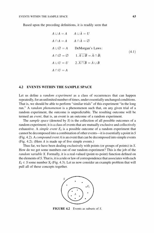
Based upon the preceding definitions, it is readily seen that
A [ A ¼ A A [ �A ¼ U
A \ A ¼ A A \ �A ¼ ˘
A [˘ ¼ A DeMorgan’s Laws :
A \˘ ¼ ˘ 1: A [ B ¼ �A \ �B;
A [ U ¼ U 2: A \ B ¼ �A [ �B
A \ U ¼ A
ð4:1Þ
4.2 EVENTS WITHIN THE SAMPLE SPACE
Let us define a random experiment as a class of occurrences that can happen
repeatedly, for an unlimited number of times, under essentially unchanged conditions.
That is, we should be able to perform “similar trials” of this experiment “in the long
run.” A random phenomenon is a phenomenon such that, on any given trial of a
random experiment, the outcome is unpredictable. The resulting outcome will be
termed an event, that is, an event is an outcome of a random experiment.
The sample space (denoted by S) is the collection of all possible outcomes of a
random experiment; it is a class of events that are mutually exclusive and collectively
exhaustive. A simple event Ei is a possible outcome of a random experiment that
cannot be decomposed into a combination of other events—it is essentially a point in S
(Fig. 4.2). A compound event A is an event that can be decomposed into simple events
(Fig. 4.2). (Here A is made up of five simple events.)
Thus far, we have been dealing exclusively with points (or groups of points) in S.
How do we get some numbers out of our random experiment? This is the job of the
random variable X. Formally, it is a real-valued (point-to-point) function defined on
the elements of S. That is, it is a rule or lawof correspondence that associateswith each
Ei 2 S some number Xi (Fig. 4.3). Let us now consider an example problem that will
pull all of these concepts together.
FIGURE 4.2 Events as subsets of S.
EVENTS WITHIN THE SAMPLE SPACE 63
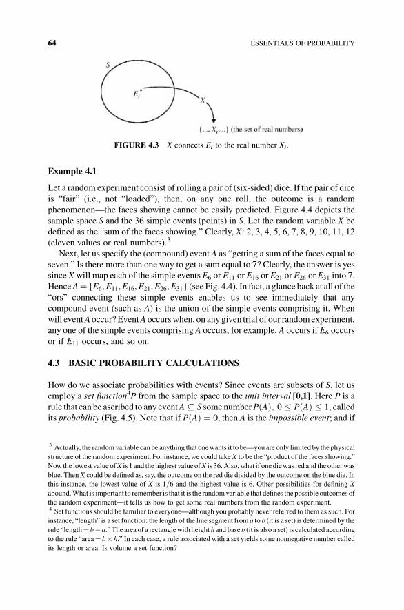
Example 4.1
Let a random experiment consist of rolling a pair of (six-sided) dice. If the pair of dice
is “fair” (i.e., not “loaded”), then, on any one roll, the outcome is a random
phenomenon—the faces showing cannot be easily predicted. Figure 4.4 depicts the
sample space S and the 36 simple events (points) in S. Let the random variable X be
defined as the “sum of the faces showing.” Clearly, X: 2, 3, 4, 5, 6, 7, 8, 9, 10, 11, 12
(eleven values or real numbers).3
Next, let us specify the (compound) event A as “getting a sum of the faces equal to
seven.” Is there more than one way to get a sum equal to 7? Clearly, the answer is yes
since X will map each of the simple events E6 or E11 or E16 or E21 or E26 or E31 into 7.
HenceA¼ {E6,E11,E16,E21,E26,E31} (see Fig. 4.4). In fact, a glance back at all of the
“ors” connecting these simple events enables us to see immediately that any
compound event (such as A) is the union of the simple events comprising it. When
will eventA occur? EventA occurswhen, on anygiven trial of our randomexperiment,
any one of the simple events comprising A occurs, for example, A occurs if E6 occurs
or if E11 occurs, and so on.
4.3 BASIC PROBABILITY CALCULATIONS
How do we associate probabilities with events? Since events are subsets of S, let us
employ a set function4P from the sample space to the unit interval [0,1]. Here P is a
rule that can be ascribed to any eventA � S some numberPðAÞ; 0 � PðAÞ � 1; calledits probability (Fig. 4.5). Note that if PðAÞ ¼ 0, then A is the impossible event; and if
3 Actually, the randomvariable can be anything that onewants it to be—youare only limited by the physical
structure of the random experiment. For instance, we could take X to be the “product of the faces showing.”
Now the lowest value ofX is 1 and the highest value ofX is 36.Also,what if one diewas red and the otherwas
blue. Then X could be defined as, say, the outcome on the red die divided by the outcome on the blue die. In
this instance, the lowest value of X is 1=6 and the highest value is 6. Other possibilities for defining X
abound.What is important to remember is that it is the randomvariable that defines the possible outcomes of
the random experiment—it tells us how to get some real numbers from the random experiment.4 Set functions should be familiar to everyone—although you probably never referred to them as such. For
instance, “length” is a set function: the length of the line segment from a to b (it is a set) is determined by the
rule “length¼ b� a.” The area of a rectanglewith height h and base b (it is also a set) is calculated according
to the rule “area¼ b� h.” In each case, a rule associated with a set yields some nonnegative number called
its length or area. Is volume a set function?
FIGURE 4.3 X connects Ei to the real number Xi:
64 ESSENTIALS OF PROBABILITY
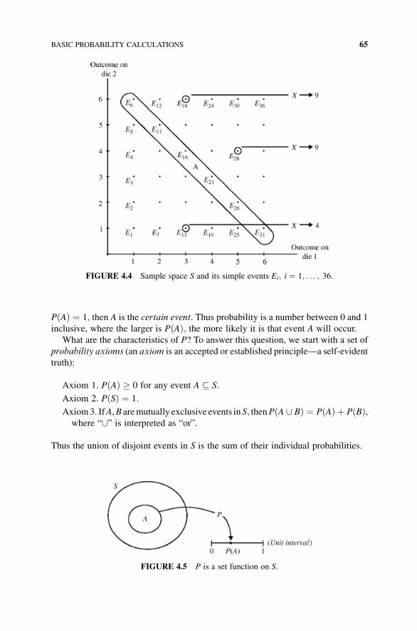
PðAÞ ¼ 1; then A is the certain event. Thus probability is a number between 0 and 1
inclusive, where the larger is PðAÞ; the more likely it is that event A will occur.
What are the characteristics of P? To answer this question, we start with a set of
probability axioms (an axiom is an accepted or established principle—a self-evident
truth):
Axiom 1. PðAÞ � 0 for any event A � S:
Axiom 2. PðSÞ ¼ 1:
Axiom3. IfA,B aremutually exclusive events in S; thenPðA [ BÞ ¼ PðAÞ þ PðBÞ,where “[” is interpreted as “or”.
Thus the union of disjoint events in S is the sum of their individual probabilities.
FIGURE 4.4 Sample space S and its simple events Ei; i ¼ 1; . . . ; 36:
FIGURE 4.5 P is a set function on S:
BASIC PROBABILITY CALCULATIONS 65
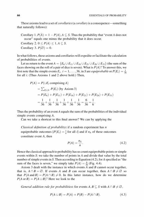
These axioms lead to a set of corollaries (a corollary is a consequence—something
that naturally follows):
Corollary 1. Pð�AÞ ¼ 1� PðAÞ;A � S: Thus the probability that “event A does not
occur” equals one minus the probability that it does occur.
Corollary 2. 0 � PðAÞ � 1;A � S:
Corollary 3. Pð˘Þ ¼ 0:
Inwhat follows, these axioms and corollaries will expedite or facilitate the calculation
of probabilities of events.
Let us return to the event A ¼ fE6 [ E11 [ E16 [ E21 [ E26 [ E31g (the sum of the
faces showing on the roll of a pair of dice is seven). What is PðAÞ? To answer this, wefirst note that the simple events Ei; i ¼ 1; . . . ; 36; in S are equiprobable or PðEiÞ ¼ 1
36
for all i. (Thus Axioms 1 and 2 above hold.) Then,
PðAÞ ¼ Pð[Ei comprising AÞ¼ P
Ei2A PðEiÞ ðby Axiom 3Þ¼ PðE6Þ þ PðE11Þ þ PðE16Þ þ PðE21Þ þ PðE26Þ þ PðE31Þ
¼ 1
36þ 1
36þ 1
36þ 1
36þ 1
36þ 1
36¼ 6
36¼ 1
6:
Thus the probability of an eventA equals the sum of the probabilities of the individual
simple events comprising A.
Can we take a shortcut to this final answer? We can by applying the
Classical definition of probability: if a random experiment has n
equiprobable outcomes [PðEiÞ ¼ 1nfor all i] and if nA of these outcomes
constitute event A, then
PðAÞ ¼ nA
n: ð4:2Þ
Hence the classical approach to probability has us count equiprobable points or simple
events within S: we take the number of points in A and divide that value by the total
number of simple events in S. Then according to Equation (4.2), forA specified as “the
sum of the faces is seven,” we simply take PðAÞ ¼ 636
(Fig. 4.4).
Axiom 3 dealt with the instance in which events A and B cannot occur together,
that is, A \ B ¼ ˘: If events A and B can occur together, then A \ B 6¼ ˘ so
that PðA and BÞ ¼ PðA \ BÞ 6¼ 0. In this latter instance, how do we determine
PðA or BÞ ¼ PðA [ BÞ? Here we look to the
General addition rule for probabilities: for events A;B � S with A \ B 6¼ ˘;
PðA [ BÞ ¼ PðAÞ þ PðBÞ � PðA \ BÞ: ð4:3Þ
66 ESSENTIALS OF PROBABILITY
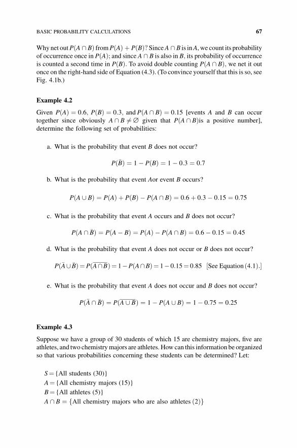
Whynet outPðA \ BÞ fromPðAÞ þ PðBÞ?SinceA \ B is inA, we count its probability
of occurrence once in PðAÞ; and since A \ B is also in B; its probability of occurrenceis counted a second time in PðBÞ: To avoid double counting PðA \ BÞ; we net it outonce on the right-hand side of Equation (4.3). (To convince yourself that this is so, see
Fig. 4.1b.)
Example 4.2
Given PðAÞ ¼ 0:6; PðBÞ ¼ 0:3; and PðA \ BÞ ¼ 0:15 [events A and B can occur
together since obviously A \ B 6¼ ˘ given that PðA \ BÞis a positive number],
determine the following set of probabilities:
a. What is the probability that event B does not occur?
Pð�BÞ ¼ 1� PðBÞ ¼ 1� 0:3 ¼ 0:7
b. What is the probability that event Aor event B occurs?
PðA [ BÞ ¼ PðAÞ þ PðBÞ � PðA \ BÞ ¼ 0:6þ 0:3� 0:15 ¼ 0:75
c. What is the probability that event A occurs and B does not occur?
PðA \ �BÞ ¼ PðA� BÞ ¼ PðAÞ � PðA \ BÞ ¼ 0:6� 0:15 ¼ 0:45
d. What is the probability that event A does not occur or B does not occur?
Pð�A[ �BÞ ¼PðA\BÞ ¼ 1�PðA\BÞ ¼ 1�0:15¼ 0:85 ½See Equation ð4:1Þ:�
e. What is the probability that event A does not occur and B does not occur?
Pð�A \ �BÞ ¼ PðA [ BÞ ¼ 1� PðA [ BÞ ¼ 1� 0:75 ¼ 0:25
Example 4.3
Suppose we have a group of 30 students of which 15 are chemistry majors, five are
athletes, and two chemistrymajors are athletes. How can this information be organized
so that various probabilities concerning these students can be determined? Let:
S¼ {All students (30)}
A¼ {All chemistry majors (15)}
B¼ {All athletes (5)}
A \ B ¼ fAll chemistry majors who are also athletes ð2Þg
BASIC PROBABILITY CALCULATIONS 67
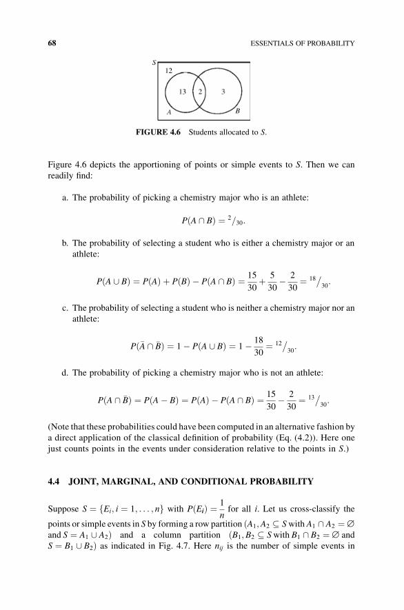
Figure 4.6 depicts the apportioning of points or simple events to S. Then we can
readily find:
a. The probability of picking a chemistry major who is an athlete:
PðA \ BÞ ¼ 230:=
b. The probability of selecting a student who is either a chemistry major or an
athlete:
PðA [ BÞ ¼ PðAÞ þ PðBÞ � PðA \ BÞ ¼ 15
30þ 5
30� 2
30¼ 18
�30:
c. The probability of selecting a student who is neither a chemistry major nor an
athlete:
Pð�A \ �BÞ ¼ 1� PðA [ BÞ ¼ 1� 18
30¼ 12
�30:
d. The probability of picking a chemistry major who is not an athlete:
PðA \ �BÞ ¼ PðA� BÞ ¼ PðAÞ � PðA \ BÞ ¼ 15
30� 2
30¼ 13
�30:
(Note that these probabilities could have been computed in an alternative fashion by
a direct application of the classical definition of probability (Eq. (4.2)). Here one
just counts points in the events under consideration relative to the points in S.)
4.4 JOINT, MARGINAL, AND CONDITIONAL PROBABILITY
Suppose S ¼ fEi; i ¼ 1; . . . ; ng with PðEiÞ ¼ 1
nfor all i. Let us cross-classify the
points or simple events in S by forming a row partition ðA1;A2 � Swith A1 \ A2 ¼ ˘and S ¼ A1 [ A2Þ and a column partition ðB1;B2 � Swith B1 \ B2 ¼ ˘ and
S ¼ B1 [ B2Þ as indicated in Fig. 4.7. Here nij is the number of simple events in
FIGURE 4.6 Students allocated to S.
68 ESSENTIALS OF PROBABILITY
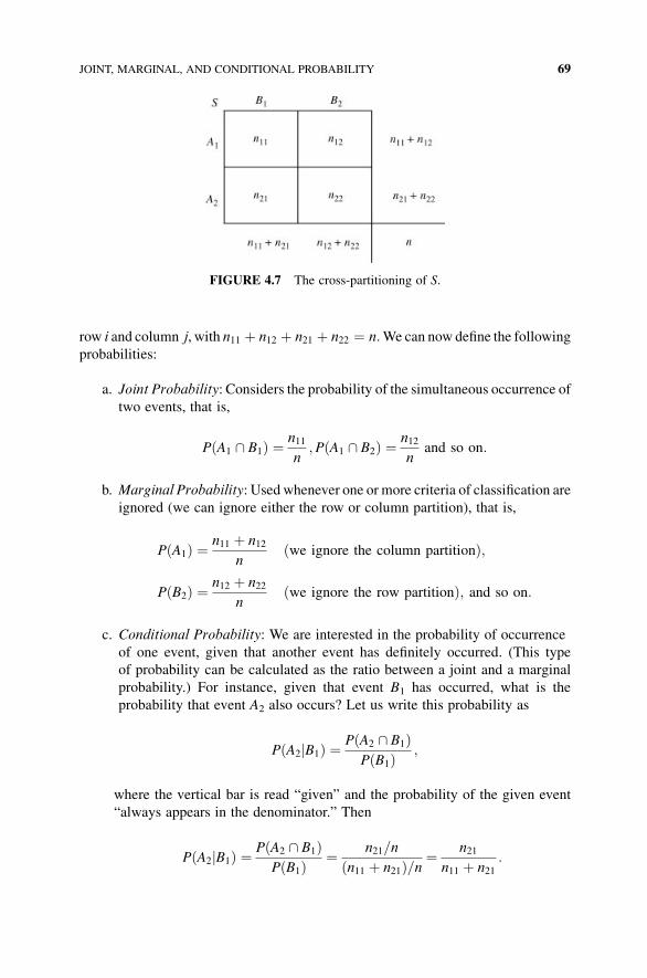
row i and column j, with n11 þ n12 þ n21 þ n22 ¼ n:We can now define the following
probabilities:
a. Joint Probability: Considers the probability of the simultaneous occurrence of
two events, that is,
PðA1 \ B1Þ ¼ n11
n;PðA1 \ B2Þ ¼ n12
nand so on:
b. Marginal Probability: Used whenever one or more criteria of classification are
ignored (we can ignore either the row or column partition), that is,
PðA1Þ ¼ n11 þ n12
nðwe ignore the column partitionÞ;
PðB2Þ ¼ n12 þ n22
nðwe ignore the row partitionÞ; and so on:
c. Conditional Probability: We are interested in the probability of occurrence
of one event, given that another event has definitely occurred. (This type
of probability can be calculated as the ratio between a joint and a marginal
probability.) For instance, given that event B1 has occurred, what is the
probability that event A2 also occurs? Let us write this probability as
PðA2jB1Þ ¼ PðA2 \ B1ÞPðB1Þ ;
where the vertical bar is read “given” and the probability of the given event
“always appears in the denominator.” Then
PðA2jB1Þ ¼ PðA2 \ B1ÞPðB1Þ ¼ n21=n
ðn11 þ n21Þ=n ¼ n21
n11 þ n21:
FIGURE 4.7 The cross-partitioning of S.
JOINT, MARGINAL, AND CONDITIONAL PROBABILITY 69
Similarly,
PðB2jA1Þ ¼ PðA1 \ B2ÞPðA1Þ ¼ n12=n
ðn11 þ n12Þ=n ¼ n12
n11 þ n12; and so on:
Let us take a shortcut to these two results. That is, we can apply the classical
definition of probability as follows. For PðA2 B1Þ;j since event B1 has occurred,
we can ignore the B2 column above. Hence the B1 column becomes our
effective sample space. Then, all we have to do is divide the number of points in
A2 \ B1 by the number of points in the given eventB1or in the effective sample
space. Thus, we can go directly to the ratio n21=ðn11 þ n21Þ: Similarly, to find
PðB2 A1Þ;j simply divide the number of elements in A1 \ B2 by the number of
elements in the given event A1 (thus the first column of the above partition
serves as the effective sample space), to which we have n12=ðn11 þ n12Þ:Since the notion of a conditional probability is of considerable importance in its own
right, let us generalize its definition. Specifically, let A;B � S with PðBÞ 6¼ 0: Then
PðAjBÞ ¼ PðA \ BÞPðBÞ : ð4:4Þ
[It is important to note that Equation (4.4) is an “evidentiary” probability; it is the
probability of A given that we “observe” B. Hence this conditional probability has
nothing to do with cause and effect.] And if PðAÞ 6¼ 0;
PðBjAÞ ¼ PðA \ BÞPðAÞ : ð4:5Þ
Given thatPðA \ BÞappears in the numerator of bothEquations (4.4) and (4.5),we can
solve for this term and form the
General multiplication rule for probabilities:
PðA \ BÞ ¼ PðBÞ PðA BÞj¼ PðAÞ PðB AÞ:j ð4:6Þ
Armed with the concept of a conditional probability, we can now introduce the notion
of independent events. Specifically, two events are independent if the occurrence of
one of them in no way affects the probability of occurrence of the other. So if events
A;B � S are independent, then PðA BÞ ¼ PðAÞj ; and PðB AÞ ¼ PðBÞ:j Clearly, these
two equalities indicate that A and B must be “mutually independent.” Under inde-
pendence, Equation (4.6) yields the following:
Test criterion for independence: if events A;B � Sare independent, then
PðA \ BÞ ¼ PðAÞ PðBÞ: ð4:7Þ
70 ESSENTIALS OF PROBABILITY
How can we generate independent events? Suppose some random experiment has
multiple trials. For example, we flip a coin five times in succession andwe let eventA1
be “the coin shows heads on the first flip,” event A2 is “the coin shows heads on the
second flip,” and so on. Since the outcome (heads or tails) on any one flip or trial does
not affect the outcome on any other trial, the trials are considered independent. But if
the trials are independent, then the events A1; . . . ;A5 must be independent. Hence
PðA1 \ A2Þ¼PðA1Þ PðA2Þ ¼ 1
2 12¼ 1
4;= PðA1 \ A2 \ A3Þ¼PðA1Þ PðA2Þ PðA3Þ¼ 1
2
� �3 ¼ 18= and so on. In this regard, independent trials will generate independent
events.
Similarly, we can generate independent events by sampling with replacement.
For instance, suppose a jar contains threewhite and seven blackmarbles. Twomarbles
are drawn at randomwith replacement (meaning that the firstmarble drawn is returned
to the jar before the second marble is drawn). What is the probability that both are
black? On draw 1, PðB1Þ ¼ 710;= on draw 2, PðB2Þ ¼ 7
10:= Hence
PðB1 \ B2Þ ¼ PðB1Þ PðB2Þ ¼ 7
10
� �2
¼ 0:49:
But what if we sampled without replacement? (Now, the first marble drawn is not
returned to the jar before the secondmarble is selected.) Obviously, the probability of
getting a black (or white)marble on the second draw depends on the color obtained on
the first draw. Clearly, there is a conditional probability calculation that must enter the
picture. Now, from Equation (4.6) we have the following:
PðB1 \ B2Þ ¼ PðB1Þ PðB2jB1Þ
¼ 7
10 69¼ 0:4667:
Here the eventsB1 and B2 are not independent; the probability thatB1 and B2 occurs is
conditional on B1 occurring. Figure 4.8 describes a decision tree diagram under
independent trials (events) or sampling with replacement. The appropriate proba-
bilities are listed beneath each node. Note that as we move along each branch, we
simply multiply the node probabilities encountered. What is the sum of the four joint
probabilities?
Figure 4.9 offers a similar diagram inwhich the events are not independent because
of sampling without replacement.
(Here too the sum of the four joint probabilities is 1.)
What if a third trial of this experiment is undertaken? Under sampling with
replacement, we can readily find, say, the following:
PðW1 \ B2 \W3Þ ¼ PðW1Þ PðB2Þ PðW3Þ ¼ 3
10 7
10 3
10¼ 0:042:
JOINT, MARGINAL, AND CONDITIONAL PROBABILITY 71
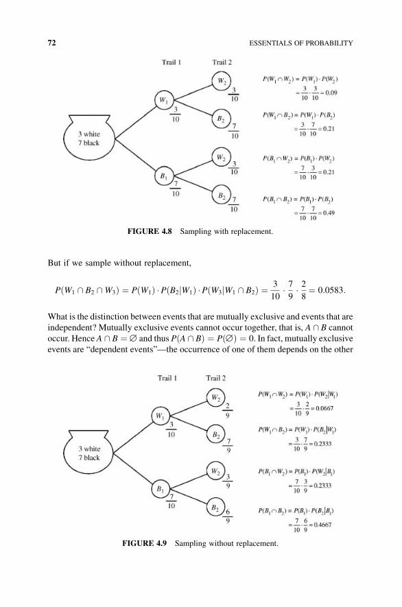
But if we sample without replacement,
PðW1 \ B2 \W3Þ ¼ PðW1Þ PðB2jW1Þ PðW3jW1 \ B2Þ ¼ 3
10 79 28¼ 0:0583:
What is the distinction between events that are mutually exclusive and events that are
independent? Mutually exclusive events cannot occur together, that is, A \ B cannot
occur. Hence A \ B ¼ ˘ and thus PðA \ BÞ ¼ Pð˘Þ ¼ 0. In fact, mutually exclusive
events are “dependent events”—the occurrence of one of them depends on the other
FIGURE 4.8 Sampling with replacement.
FIGURE 4.9 Sampling without replacement.
72 ESSENTIALS OF PROBABILITY
not occurring. However, independent events can occur together (A \ B can occur)—it
is just that the occurrence of one of them does not affect the probability of occurrence
of the other. For example, PðA BÞ ¼ PðAÞj so that PðA \ BÞ ¼ PðAÞ PðBÞ.
4.5 SOURCES OF PROBABILITIES
Let us now examine the various ways in which probabilities are determined. Two
broad categories of probabilities are typically recognized: objective probability
versus subjective probability. Moreover, under the objective heading, we have the
classical approach versus the empirical determination of probability.
The classical approach utilities a priori (before the fact) knowledge, that is, we can
determine a theoretical probability by counting points or simple events within S.
Clearly, this approach utilizes the physical structure of an implied experiment and is
used when we have n equiprobable simple events in S.
An empirical probability utilizes a posteriori (after the fact) knowledge; it makes
use of accumulated or historical experience or is determined by actually performing a
random experiment. That is, we can compute the relative frequency of an event via a
random experiment. Specifically, if A is an event for a random experiment and if that
experiment is repeated n times and A is observed in nA of the n repetitions, then the
relative frequency of event A is nA=n. What is the connection between relative
frequency and probability? The link is provided by the frequency limit principle: if in a
large number n of independent repetitions of a random experiment the relative
frequencies nA=n of some event A approach a number PðAÞ, then this number is
ascribed to A as its probability, that is,
limn!¥
nA
n¼ PðAÞ or nA
n!PðAÞ as n!¥:
Here PðAÞ is a long-run stable value that the relative frequencies approach—it is the
expected limit of nA=n (Fig. 4.10). (The reader may want to flip a coin, say, 30 times
and, for the event A: the coin shows heads, calculate nA=n:While n ¼ 30 is certainly
not the “ long run,” one can get the “flavor” of the frequency limit principle by
performing this rather trivial random experiment.)
Sometimes, the frequency limit principle is termed as the law of large numbers: if
PðAÞ ¼ p and n independent repetitions of a random experiment are made, then the
probability that nA=n differs from p by any amount, however small, tends to one as n
increases without bound, That is,
PnA
n� p
������Ge
� ! 1 as n!¥;
where e is an arbitrary small positive number. It is important to note that the
law of large numbers does not state that nA=n is necessarily getting closer and
SOURCES OF PROBABILITIES 73
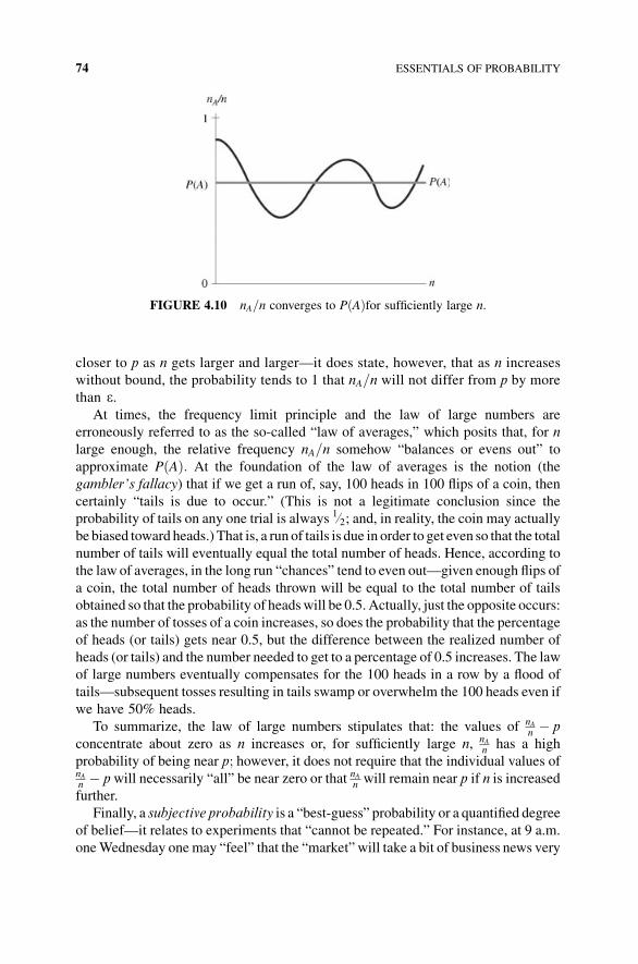
closer to p as n gets larger and larger—it does state, however, that as n increases
without bound, the probability tends to 1 that nA=n will not differ from p by more
than e.At times, the frequency limit principle and the law of large numbers are
erroneously referred to as the so-called “law of averages,” which posits that, for n
large enough, the relative frequency nA=n somehow “balances or evens out” to
approximate PðAÞ: At the foundation of the law of averages is the notion (the
gambler’s fallacy) that if we get a run of, say, 100 heads in 100 flips of a coin, then
certainly “tails is due to occur.” (This is not a legitimate conclusion since the
probability of tails on any one trial is always 1=2; and, in reality, the coin may actually
be biased toward heads.) That is, a run of tails is due in order to get even so that the total
number of tails will eventually equal the total number of heads. Hence, according to
the law of averages, in the long run “chances” tend to even out—given enough flips of
a coin, the total number of heads thrown will be equal to the total number of tails
obtained so that the probability of headswill be 0.5. Actually, just the opposite occurs:
as the number of tosses of a coin increases, so does the probability that the percentage
of heads (or tails) gets near 0.5, but the difference between the realized number of
heads (or tails) and the number needed to get to a percentage of 0.5 increases. The law
of large numbers eventually compensates for the 100 heads in a row by a flood of
tails—subsequent tosses resulting in tails swamp or overwhelm the 100 heads even if
we have 50% heads.
To summarize, the law of large numbers stipulates that: the values of nAn� p
concentrate about zero as n increases or, for sufficiently large n, nAnhas a high
probability of being near p; however, it does not require that the individual values ofnAn� pwill necessarily “all” be near zero or that nA
nwill remain near p if n is increased
further.
Finally, a subjective probability is a “best-guess” probability or a quantified degree
of belief—it relates to experiments that “cannot be repeated.” For instance, at 9 a.m.
oneWednesday onemay “feel” that the “market” will take a bit of business news very
FIGURE 4.10 nA=n converges to PðAÞfor sufficiently large n.
74 ESSENTIALS OF PROBABILITY
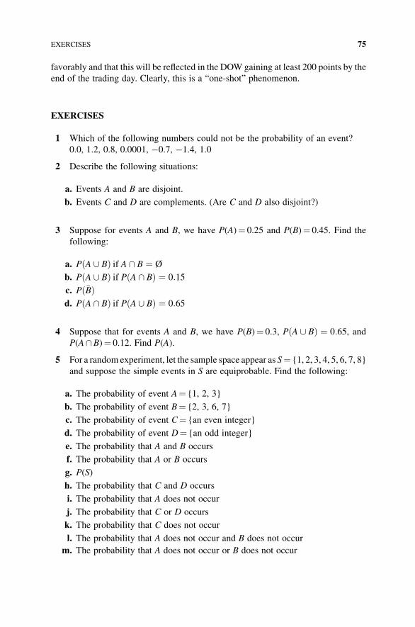
favorably and that this will be reflected in the DOW gaining at least 200 points by the
end of the trading day. Clearly, this is a “one-shot” phenomenon.
EXERCISES
1 Which of the following numbers could not be the probability of an event?
0.0, 1.2, 0.8, 0.0001, �0.7, �1.4, 1.0
2 Describe the following situations:
a. Events A and B are disjoint.
b. Events C and D are complements. (Are C and D also disjoint?)
3 Suppose for events A and B, we have P(A)¼ 0.25 and P(B)¼ 0.45. Find the
following:
a. PðA [ BÞ if A \ B ¼ Ø
b. PðA [ BÞ if PðA \ BÞ ¼ 0:15
c. Pð�BÞd. PðA \ BÞ if PðA [ BÞ ¼ 0:65
4 Suppose that for events A and B, we have P(B)¼ 0.3, PðA [ BÞ ¼ 0:65, andP(A\B)¼ 0.12. Find P(A).
5 For a random experiment, let the sample space appear as S¼ {1, 2, 3, 4, 5, 6, 7, 8}
and suppose the simple events in S are equiprobable. Find the following:
a. The probability of event A¼ {1, 2, 3}
b. The probability of event B¼ {2, 3, 6, 7}
c. The probability of event C¼ {an even integer}
d. The probability of event D¼ {an odd integer}
e. The probability that A and B occurs
f. The probability that A or B occurs
g. P(S)
h. The probability that C and D occurs
i. The probability that A does not occur
j. The probability that C or D occurs
k. The probability that C does not occur
l. The probability that A does not occur and B does not occur
m. The probability that A does not occur or B does not occur
EXERCISES 75
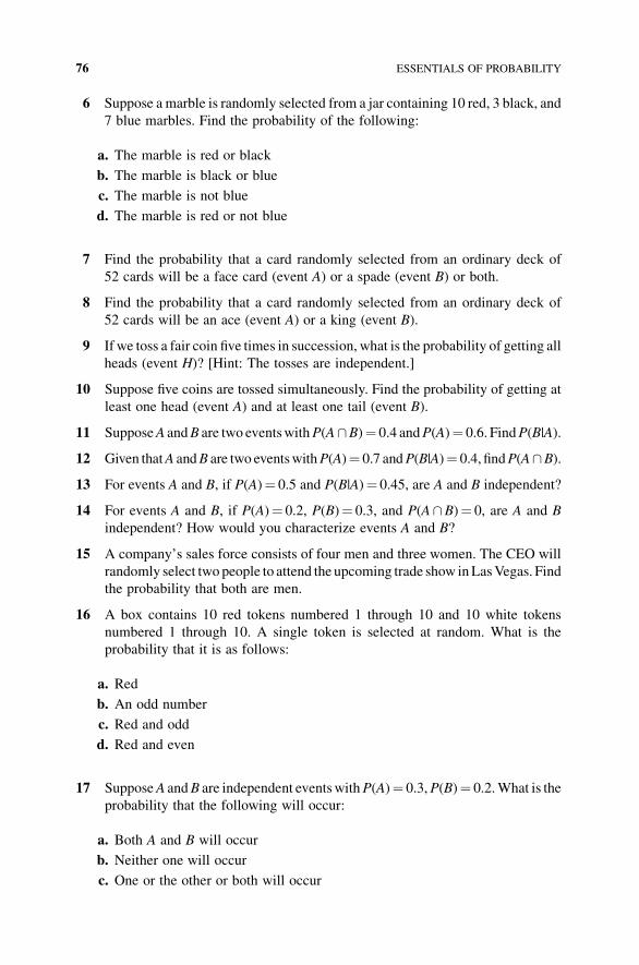
6 Suppose a marble is randomly selected from a jar containing 10 red, 3 black, and
7 blue marbles. Find the probability of the following:
a. The marble is red or black
b. The marble is black or blue
c. The marble is not blue
d. The marble is red or not blue
7 Find the probability that a card randomly selected from an ordinary deck of
52 cards will be a face card (event A) or a spade (event B) or both.
8 Find the probability that a card randomly selected from an ordinary deck of
52 cards will be an ace (event A) or a king (event B).
9 If we toss a fair coin five times in succession, what is the probability of getting all
heads (event H)? [Hint: The tosses are independent.]
10 Suppose five coins are tossed simultaneously. Find the probability of getting at
least one head (event A) and at least one tail (event B).
11 SupposeA andB are two eventswithP(A\B)¼ 0.4 andP(A)¼ 0.6. FindP(B|A).
12 Given thatA andB are two eventswithP(A)¼ 0.7 andP(B|A)¼ 0.4, findP(A\B).
13 For events A and B, if P(A)¼ 0.5 and P(B|A)¼ 0.45, are A and B independent?
14 For events A and B, if P(A)¼ 0.2, P(B)¼ 0.3, and P(A\B)¼ 0, are A and B
independent? How would you characterize events A and B?
15 A company’s sales force consists of four men and three women. The CEO will
randomly select two people to attend the upcoming trade show inLasVegas. Find
the probability that both are men.
16 A box contains 10 red tokens numbered 1 through 10 and 10 white tokens
numbered 1 through 10. A single token is selected at random. What is the
probability that it is as follows:
a. Red
b. An odd number
c. Red and odd
d. Red and even
17 SupposeA andB are independent eventswithP(A)¼ 0.3,P(B)¼ 0.2.What is the
probability that the following will occur:
a. Both A and B will occur
b. Neither one will occur
c. One or the other or both will occur
76 ESSENTIALS OF PROBABILITY
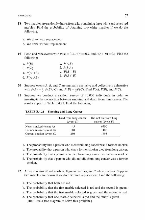
18 Twomarbles are randomly drawn from a jar containing threewhite and seven red
marbles. Find the probability of obtaining two white marbles if we do the
following:
a. We draw with replacement
b. We draw without replacement
19 Let A and B be events with P(A)¼ 0.3, P(B)¼ 0.7, and P(A\B)¼ 0.1. Find the
following:
a. P �Bð Þb. P �Að Þc. P �A \ �Bð Þd. P A [ Bð Þ
e. P(A|B)
f. P �B Aj Þðg. P A \ �Bð Þh. P �A \ Bð Þ
20 Suppose events A, B, and C are mutually exclusive and collectively exhaustive
with P Að Þ ¼ 12; P B [ Cð Þ and P Bð Þ ¼ 1
2P Cð Þ. Find P(A), P(B), and P(C).
21 Suppose we conduct a random survey of 10,000 individuals in order to
investigate the connection between smoking and death from lung cancer. The
results appear in Table E.4.21. Find the following:
a. The probability that a person who died from lung cancer was a former smoker.
b. The probability that a person who was a former smoker died from lung cancer.
c. The probability that a person who died from lung cancer was never a smoker.
d. The probability that a person who did not die from lung cancer was a former
smoker.
22 A bag contains 20 red marbles, 8 green marbles, and 7 white marbles. Suppose
two marbles are drawn at random without replacement. Find the following:
a. The probability that both are red.
b. The probability that the first marble selected is red and the second is green.
c. The probability that the first marble selected is green and the second is red.
d. The probability that one marble selected is red and the other is green.
[Hint: Use a tree diagram to solve this problem.]
TABLE E.4.21 Smoking and Lung Cancer
Died from lung cancer
(event D)
Did not die from lung
cancer (event �D)
Never smoked (event A) 45 6500
Former smoker (event B) 110 1400
Current smoker (event C) 250 1695
EXERCISES 77
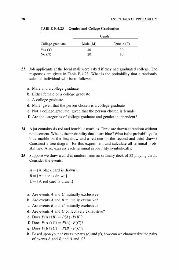
23 Job applicants at the local mall were asked if they had graduated college. The
responses are given in Table E.4.23. What is the probability that a randomly
selected individual will be as follows:
a. Male and a college graduate
b. Either female or a college graduate
c. A college graduate
d. Male, given that the person chosen is a college graduate
e. Not a college graduate, given that the person chosen is female
f. Are the categories of college graduate and gender independent?
24 A jar contains six red and four blue marbles. Three are drawn at randomwithout
replacement.What is the probability that all are blue?What is the probability of a
blue marble on the first draw and a red one on the second and third draws?
Construct a tree diagram for this experiment and calculate all terminal prob-
abilities. Also, express each terminal probability symbolically.
25 Suppose we draw a card at random from an ordinary deck of 52 playing cards.
Consider the events:
A¼ {A black card is drawn}
B¼ {An ace is drawn}
C¼ {A red card is drawn}
a. Are events A and C mutually exclusive?
b. Are events A and B mutually exclusive?
c. Are events B and C mutually exclusive?
d. Are events A and C collectively exhaustive?
e. Does P A \ Bð Þ ¼ P Að Þ P Bð Þ?f. Does P A \ Cð Þ ¼ P Að Þ P Cð Þ?g. Does P B \ Cð Þ ¼ P Bð Þ P Cð Þ?h. Based upon your answers to parts (e) and (f), how can we characterize the pairs
of events A and B and A and C?
TABLE E.4.23 Gender and College Graduation
Gender
College graduate Male (M) Female (F)
Yes (Y) 40 30
No (N) 20 10
78 ESSENTIALS OF PROBABILITY
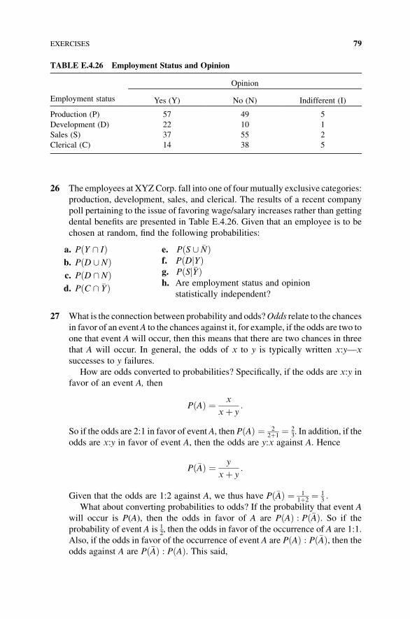
26 The employees at XYZCorp. fall into one of four mutually exclusive categories:
production, development, sales, and clerical. The results of a recent company
poll pertaining to the issue of favoring wage/salary increases rather than getting
dental benefits are presented in Table E.4.26. Given that an employee is to be
chosen at random, find the following probabilities:
a. P Y \ Ið Þb. P D [ Nð Þc. P D \ Nð Þd. P C \ �Yð Þ
e. P S [ �Nð Þf. P D Yj Þðg. P S �Yj Þðh. Are employment status and opinion
statistically independent?
27 What is the connection between probability and odds?Odds relate to the chances
in favor of an eventA to the chances against it, for example, if the odds are two to
one that event A will occur, then this means that there are two chances in three
that A will occur. In general, the odds of x to y is typically written x:y—x
successes to y failures.
How are odds converted to probabilities? Specifically, if the odds are x:y in
favor of an event A, then
P Að Þ ¼ x
xþ y:
So if the odds are 2:1 in favor of event A, then P Að Þ ¼ 22þ1
¼ 23. In addition, if the
odds are x:y in favor of event A, then the odds are y:x against A. Hence
P �Að Þ ¼ y
xþ y:
Given that the odds are 1:2 against A, we thus have P �Að Þ ¼ 11þ2
¼ 13:
What about converting probabilities to odds? If the probability that event A
will occur is P(A), then the odds in favor of A are P Að Þ : P �Að Þ. So if the
probability of event A is 12, then the odds in favor of the occurrence of A are 1:1.
Also, if the odds in favor of the occurrence of event A are P Að Þ : P �Að Þ, then theodds against A are P �Að Þ : P Að Þ. This said,
TABLE E.4.26 Employment Status and Opinion
Employment status
Opinion
Yes (Y) No (N) Indifferent (I)
Production (P) 57 49 5
Development (D) 22 10 1
Sales (S) 37 55 2
Clerical (C) 14 38 5
EXERCISES 79

a. If the odds are 6:4 thatMary’s boyfriendwill proposemarriage tonight, what is
the probability that a proposal occurs?
b. What is the probability that a proposal will not be made? [Hint: The odds are
4:6 against the proposal.]
c. If Mary awoke with the feeling that the probability of her boyfriend proposing
marriage that evening is 45, what are the odds that a proposal will occur?
d. What are the odds that a proposal will not occur?
80 ESSENTIALS OF PROBABILITY
5DISCRETE PROBABILITYDISTRIBUTIONS AND THEIRPROPERTIES
5.1 THE DISCRETE PROBABILITY DISTRIBUTION
A probability distribution is termed discrete if the underlying random variable X is
discrete. (Remember that a random variable X is a real-valued function defined on the
elements of a sample space S—its role is to define the possible outcomes of a random
experiment.) In this regard, the number of values thatX can assume forms a countable
set: either there exists a finite number of elements or the elements are countably
infinite (can be put in one-to-one correspondence with the positive integers or
counting numbers).
For instance, let X represent the outcome (the face showing) on the roll of a single
six-sided die. ThenX¼ {1, 2, 3, 4, 5, 6}—theX values form a countable set. However,
what if we roll the die repeatedly until a five appears for the first time? Then if X
represents the number of rolls it takes to get a five for the first time, clearly, X¼ {1, 2,
3, . . .}, that is, the X values form a countably infinite set.
This said, a discrete probability distribution is a distribution exhibiting the values
of a discrete randomvariableX and their associated probabilities. In order to construct
a discrete probability distribution, we need three pieces of information:
Statistical Inference: A Short Course, First Edition. Michael J. Panik.� 2012 John Wiley & Sons, Inc. Published 2012 by John Wiley & Sons, Inc.
81
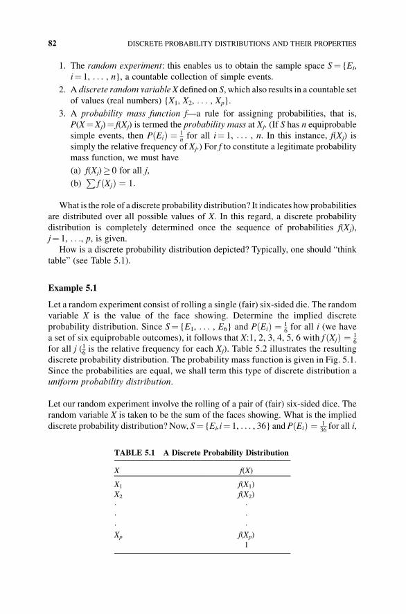
1. The random experiment: this enables us to obtain the sample space S¼ {Ei,
i¼ 1, . . . , n}, a countable collection of simple events.
2. A discrete random variable X defined on S, which also results in a countable set
of values (real numbers) {X1, X2, . . . , Xp}.
3. A probability mass function f—a rule for assigning probabilities, that is,
P(X¼Xj)¼ f(Xj) is termed the probability mass at Xj. (If S has n equiprobable
simple events, then PðEiÞ ¼ 1nfor all i¼ 1, . . . , n. In this instance, f(Xj) is
simply the relative frequency of Xj.) For f to constitute a legitimate probability
mass function, we must have
(a) f(Xj)� 0 for all j,
(b)P
f ðXjÞ ¼ 1:
What is the role of a discrete probability distribution? It indicates howprobabilities
are distributed over all possible values of X. In this regard, a discrete probability
distribution is completely determined once the sequence of probabilities f(Xj),
j¼ 1, . . ., p, is given.How is a discrete probability distribution depicted? Typically, one should “think
table” (see Table 5.1).
Example 5.1
Let a random experiment consist of rolling a single (fair) six-sided die. The random
variable X is the value of the face showing. Determine the implied discrete
probability distribution. Since S¼ {E1, . . . , E6} and PðEiÞ ¼ 16for all i (we have
a set of six equiprobable outcomes), it follows that X:1, 2, 3, 4, 5, 6 with f ðXjÞ ¼ 16
for all j (16is the relative frequency for each Xj). Table 5.2 illustrates the resulting
discrete probability distribution. The probability mass function is given in Fig. 5.1.
Since the probabilities are equal, we shall term this type of discrete distribution a
uniform probability distribution.
Let our random experiment involve the rolling of a pair of (fair) six-sided dice. The
random variable X is taken to be the sum of the faces showing. What is the implied
discrete probability distribution? Now, S¼ {Ei,i¼ 1, . . . , 36} and PðEiÞ ¼ 136for all i,
TABLE 5.1 A Discrete Probability Distribution
X f(X)
X1 f(X1)
X2 f(X2)
� �� �� �Xp f(Xp)
1
82 DISCRETE PROBABILITY DISTRIBUTIONS AND THEIR PROPERTIES
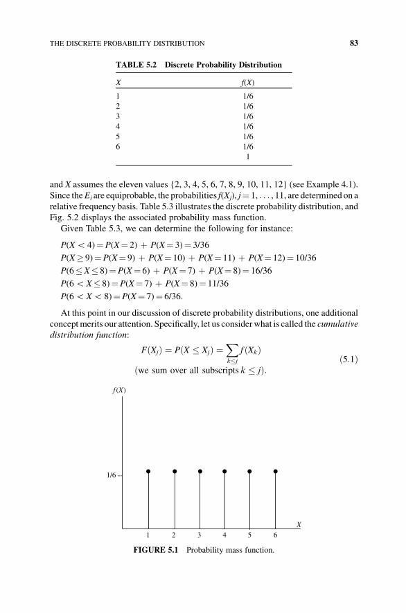
and X assumes the eleven values {2, 3, 4, 5, 6, 7, 8, 9, 10, 11, 12} (see Example 4.1).
Since theEi are equiprobable, the probabilities f(Xj), j¼ 1, . . . , 11, are determined on a
relative frequency basis. Table 5.3 illustrates the discrete probability distribution, and
Fig. 5.2 displays the associated probability mass function.
Given Table 5.3, we can determine the following for instance:
P(XG 4)¼P(X¼ 2) þ P(X¼ 3)¼ 3/36
P(X� 9)¼P(X¼ 9) þ P(X¼ 10) þ P(X¼ 11) þ P(X¼ 12)¼ 10/36
P(6�X� 8)¼P(X¼ 6) þ P(X¼ 7) þ P(X¼ 8)¼ 16/36
P(6GX� 8)¼P(X¼ 7) þ P(X¼ 8)¼ 11/36
P(6GXG 8)¼P(X¼ 7)¼ 6/36.
At this point in our discussion of discrete probability distributions, one additional
conceptmerits our attention. Specifically, let us considerwhat is called the cumulative
distribution function:
FðXjÞ ¼ PðX � XjÞ ¼X
k�j
f Xkð Þ
ðwe sum over all subscripts k � jÞ:ð5:1Þ
TABLE 5.2 Discrete Probability Distribution
X f(X)
1 1/6
2 1/6
3 1/6
4 1/6
5 1/6
6 1/6
1
f (X)
1 2 3 4 5 6
X
1/6 --
FIGURE 5.1 Probability mass function.
THE DISCRETE PROBABILITY DISTRIBUTION 83
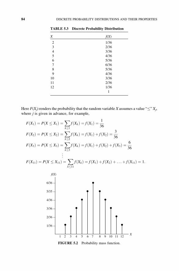
Here F(Xj) renders the probability that the random variable X assumes a value “�” Xj,
where j is given in advance, for example,
FðX1Þ ¼ PðX � X1Þ ¼X
k�1
f Xkð Þ ¼ f ðX1Þ ¼ 1
36
FðX2Þ ¼ PðX � X2Þ ¼X
k�2
f Xkð Þ ¼ f ðX1Þ þ f ðX2Þ ¼ 3
36
FðX3Þ ¼ PðX � X3Þ ¼X
k�3
f Xkð Þ ¼ f ðX1Þ þ f ðX2Þ þ f ðX3Þ ¼ 6
36
..
.
FðX11Þ ¼ PðX � X11Þ ¼X
k�11
f Xkð Þ ¼ f ðX1Þ þ f ðX2Þ þ . . .þ f ðX11Þ ¼ 1:
TABLE 5.3 Discrete Probability Distribution
X f(X)
2 1/36
3 2/36
4 3/36
5 4/36
6 5/36
7 6/36
8 5/36
9 4/36
10 3/36
11 2/36
12 1/36
1
f(X)
6/36 --
5/35 --
4/36 --
3/36 --
2/36 --
1/36 --
X1 2 3 4 5 6 7 8 9 10 11 12
FIGURE 5.2 Probability mass function.
84 DISCRETE PROBABILITY DISTRIBUTIONS AND THEIR PROPERTIES
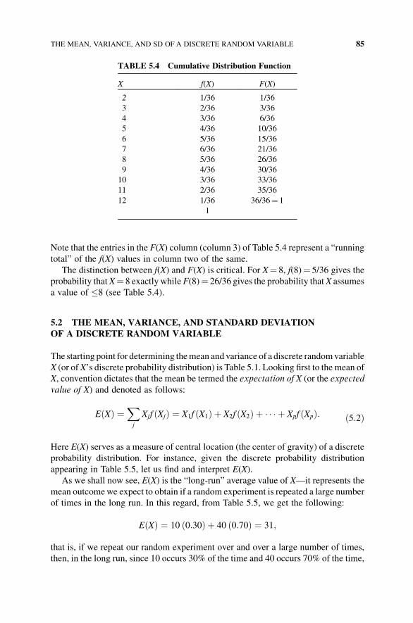
Note that the entries in the F(X) column (column 3) of Table 5.4 represent a “running
total” of the f(X) values in column two of the same.
The distinction between f(X) and F(X) is critical. For X¼ 8, f(8)¼ 5/36 gives the
probability thatX¼ 8 exactly whileF(8)¼ 26/36 gives the probability thatX assumes
a value of �8 (see Table 5.4).
5.2 THE MEAN, VARIANCE, AND STANDARD DEVIATION
OF A DISCRETE RANDOM VARIABLE
The starting point for determining themean and variance of a discrete randomvariable
X (or of X’s discrete probability distribution) is Table 5.1. Looking first to the mean of
X, convention dictates that the mean be termed the expectation of X (or the expected
value of X) and denoted as follows:
EðXÞ ¼X
j
Xjf ðXjÞ ¼ X1f ðX1Þ þ X2f ðX2Þ þ � � � þ Xpf ðXpÞ: ð5:2Þ
Here E(X) serves as a measure of central location (the center of gravity) of a discrete
probability distribution. For instance, given the discrete probability distribution
appearing in Table 5.5, let us find and interpret E(X).
As we shall now see, E(X) is the “long-run” average value of X—it represents the
mean outcomewe expect to obtain if a random experiment is repeated a large number
of times in the long run. In this regard, from Table 5.5, we get the following:
EðXÞ ¼ 10 ð0:30Þ þ 40 ð0:70Þ ¼ 31;
that is, if we repeat our random experiment over and over a large number of times,
then, in the long run, since 10 occurs 30% of the time and 40 occurs 70% of the time,
TABLE 5.4 Cumulative Distribution Function
X f(X) F(X)
2 1/36 1/36
3 2/36 3/36
4 3/36 6/36
5 4/36 10/36
6 5/36 15/36
7 6/36 21/36
8 5/36 26/36
9 4/36 30/36
10 3/36 33/36
11 2/36 35/36
12 1/36 36/36¼ 1
1
THE MEAN, VARIANCE, AND SD OF A DISCRETE RANDOM VARIABLE 85
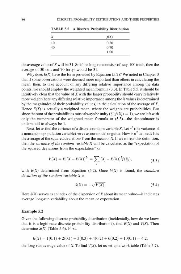
the average value ofXwill be 31. So if the long run consists of, say, 100 trials, then the
average of 30 tens and 70 fortys would be 31.
Why does E(X) have the form provided by Equation (5.2)? We noted in Chapter 3
that if some observations were deemed more important than others in calculating the
mean, then, to take account of any differing relative importance among the data
points, we should employ the weighted mean formula (3.3). In Table 5.5, it should be
intuitively clear that the value of X with the larger probability should carry relatively
moreweight (here any differing relative importance among theX values is determined
by the magnitudes of their probability values) in the calculation of the average of X.
Hence E(X) is actually a weighted mean, where the weights are probabilities. But
since the sumof the probabilitiesmust always be unity (P
f ðXjÞ ¼ 1),we are left with
only the numerator of the weighted mean formula or (5.3)—the denominator is
understood to always be 1.
Next, let us find thevariance of a discrete randomvariableX. Lets2 (the variance ofa nonrandompopulationvariable) serve as ourmodel or guide. How iss2 defined? It isthe average of the squared deviations from the mean of X. If we mirror this definition,
then the variance of the random variable X will be calculated as the “expectation of
the squared deviations from the expectation” or
VðXÞ ¼ E½ðX � EðXÞÞ2� ¼X
j
ðXj � EðXÞÞ2f ðXjÞ; ð5:3Þ
with E(X) determined from Equation (5.2). Once V(X) is found, the standard
deviation of the random variable X is
SðXÞ ¼ þffiffiffiffiffiffiffiffiffiffiffiffiVðXÞ:
pð5:4Þ
Here S(X) serves as an index of the dispersion of X about its mean value—it indicates
average long-run variability about the mean or expectation.
Example 5.2
Given the following discrete probability distribution (incidentally, how do we know
that it is a legitimate discrete probability distribution?), find E(X) and V(X). Then
determine S(X) (Table 5.6). First,
EðXÞ ¼ 1ð0:1Þ þ 2ð0:1Þ þ 3ð0:3Þ þ 4ð0:2Þ þ 6ð0:2Þ þ 10ð0:1Þ ¼ 4:2;
the long-run average value of X. To find V(X), let us set up a work table (Table 5.7).
TABLE 5.5 A Discrete Probability Distribution
X f(X)
10 0.30
40 0.70
1.00
86 DISCRETE PROBABILITY DISTRIBUTIONS AND THEIR PROPERTIES
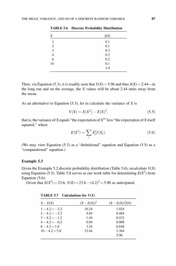
Then, via Equation (5.3), it is readily seen that V(X)¼ 5.96 and thus S(X)¼ 2.44—in
the long run and on the average, the X values will be about 2.44 units away from
the mean.
As an alternative to Equation (5.3), let us calculate the variance of X is
VðXÞ ¼ EðX2Þ � EðXÞ2; ð5:5Þthat is, the variance ofX equals “the expectation ofX2” less “the expectation ofX itself
squared,” where
EðX2Þ ¼X
j
X2j f ðXjÞ: ð5:6Þ
(We may view Equation (5.3) as a “definitional” equation and Equation (5.5) as a
“computational” equation.)
Example 5.3
Given the Example 5.2 discrete probability distribution (Table 5.6), recalculate V(X)
using Equation (5.5). Table 5.8 serves as our work table for determining E(X2) from
Equation (5.6).
Given that E(X2)¼ 23.6, V(X)¼ 23.6� (4.2)2¼ 5.96 as anticipated.
TABLE 5.6 Discrete Probability Distribution
X f(X)
1 0.1
2 0.1
3 0.3
4 0.2
6 0.2
10 0.1
1.0
TABLE 5.7 Calculations for V(X)
X�E(X) (X�E(X))2 (X�E(X))2f(X)
1� 4.2¼�3.2 10.24 1.024
2� 4.2¼�2.2 4.84 0.484
3� 4.2¼�1.2 1.44 0.432
4� 4.2¼�0.2 0.04 0.008
6� 4.2¼ 1.8 3.24 0.648
10� 4.2¼ 5.8 33.64 3.364
5.96
THE MEAN, VARIANCE, AND SD OF A DISCRETE RANDOM VARIABLE 87
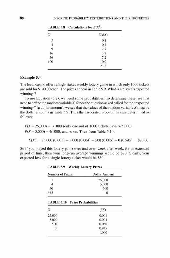
Example 5.4
The local casino offers a high-stakes weekly lottery game in which only 1000 tickets
are sold for $100.00 each. The prizes appear in Table 5.9. What is a player’s expected
winnings?
To use Equation (5.2), we need some probabilities. To determine these, we first
need to define the randomvariableX. Since the question asked called for the “expected
winnings” (a dollar amount), we see that the values of the random variable Xmust be
the dollar amounts in Table 5.9. Thus the associated probabilities are determined as
follows:
P(X¼ 25,000)¼ 1/1000 (only one out of 1000 tickets pays $25,000),
P(X¼ 5,000)¼ 4/1000, and so on. Then from Table 5.10,
EðXÞ ¼ 25;000 ð0:001Þ þ 5;000 ð0:004Þ þ 500 ð0:005Þ þ 0 ð0:945Þ ¼ $70:00:
So if you played this lottery game over and over, week after week, for an extended
period of time, then your long-run average winnings would be $70. Clearly, your
expected loss for a single lottery ticket would be $30.
TABLE 5.8 Calculations for E(X2)
X2 X2f(X)
1 0.1
4 0.4
9 2.7
16 3.2
36 7.2
100 10.0
23.6
TABLE 5.9 Weekly Lottery Prizes
Number of Prizes Dollar Amount
1 25,000
4 5,000
50 500
945 0
TABLE 5.10 Prize Probabilities
X f(X)
25,000 0.001
5,000 0.004
500 0.050
0 0.945
1.000
88 DISCRETE PROBABILITY DISTRIBUTIONS AND THEIR PROPERTIES
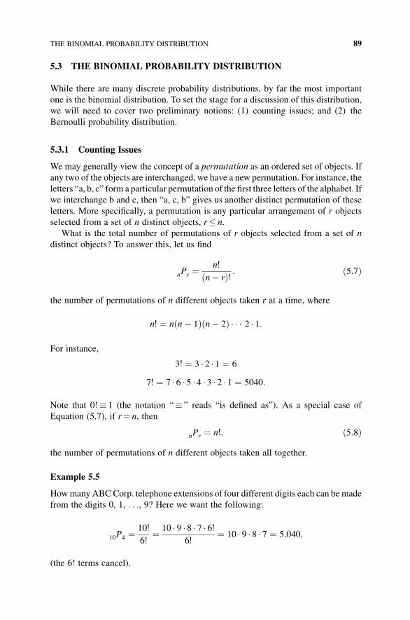
5.3 THE BINOMIAL PROBABILITY DISTRIBUTION
While there are many discrete probability distributions, by far the most important
one is the binomial distribution. To set the stage for a discussion of this distribution,
we will need to cover two preliminary notions: (1) counting issues; and (2) the
Bernoulli probability distribution.
5.3.1 Counting Issues
We may generally view the concept of a permutation as an ordered set of objects. If
any two of the objects are interchanged, we have a new permutation. For instance, the
letters “a, b, c” form a particular permutation of the first three letters of the alphabet. If
we interchange b and c, then “a, c, b” gives us another distinct permutation of these
letters. More specifically, a permutation is any particular arrangement of r objects
selected from a set of n distinct objects, r� n.
What is the total number of permutations of r objects selected from a set of n
distinct objects? To answer this, let us find
nPr ¼n!
ðn� rÞ! : ð5:7Þ
the number of permutations of n different objects taken r at a time, where
n! ¼ n n� 1ð Þ n� 2ð Þ � � � 2 � 1:
For instance,
3! ¼ 3 � 2 � 1 ¼ 6
7! ¼ 7 � 6 � 5 � 4 � 3 � 2 � 1 ¼ 5040:
Note that 0!� 1 (the notation “� ” reads “is defined as”). As a special case of
Equation (5.7), if r¼ n, then
nPr ¼ n!; ð5:8Þ
the number of permutations of n different objects taken all together.
Example 5.5
HowmanyABCCorp. telephone extensions of four different digits each can be made
from the digits 0, 1, . . ., 9? Here we want the following:
10P4 ¼10!
6!¼ 10 � 9 � 8 � 7 � 6!
6!¼ 10 � 9 � 8 � 7 ¼ 5;040;
(the 6! terms cancel).
THE BINOMIAL PROBABILITY DISTRIBUTION 89
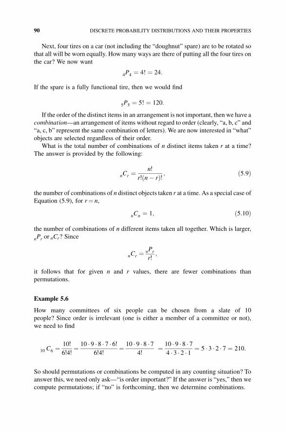
Next, four tires on a car (not including the “doughnut” spare) are to be rotated so
that all will be worn equally. How many ways are there of putting all the four tires on
the car? We now want
4P4 ¼ 4! ¼ 24:
If the spare is a fully functional tire, then we would find
5P5 ¼ 5! ¼ 120:
If the order of the distinct items in an arrangement is not important, then we have a
combination—an arrangement of items without regard to order (clearly, “a, b, c” and
“a, c, b” represent the same combination of letters). We are now interested in “what”
objects are selected regardless of their order.
What is the total number of combinations of n distinct items taken r at a time?
The answer is provided by the following:
nCr ¼n!
r!ðn� rÞ! ; ð5:9Þ
the number of combinations of n distinct objects taken r at a time. As a special case of
Equation (5.9), for r¼ n,
nCn ¼ 1; ð5:10Þ
the number of combinations of n different items taken all together. Which is larger,
nPr or nCr? Since
nCr ¼ nPr
r!;
it follows that for given n and r values, there are fewer combinations than
permutations.
Example 5.6
How many committees of six people can be chosen from a slate of 10
people? Since order is irrelevant (one is either a member of a committee or not),
we need to find
10 C6 ¼10!
6!4!¼ 10 � 9 � 8 � 7 � 6!
6!4!¼ 10 � 9 � 8 � 7
4!¼ 10 � 9 � 8 � 7
4 � 3 � 2 � 1 ¼ 5 � 3 � 2 � 7 ¼ 210:
So should permutations or combinations be computed in any counting situation? To
answer this, we need only ask—“is order important?” If the answer is “yes,” then we
compute permutations; if “no” is forthcoming, then we determine combinations.
90 DISCRETE PROBABILITY DISTRIBUTIONS AND THEIR PROPERTIES
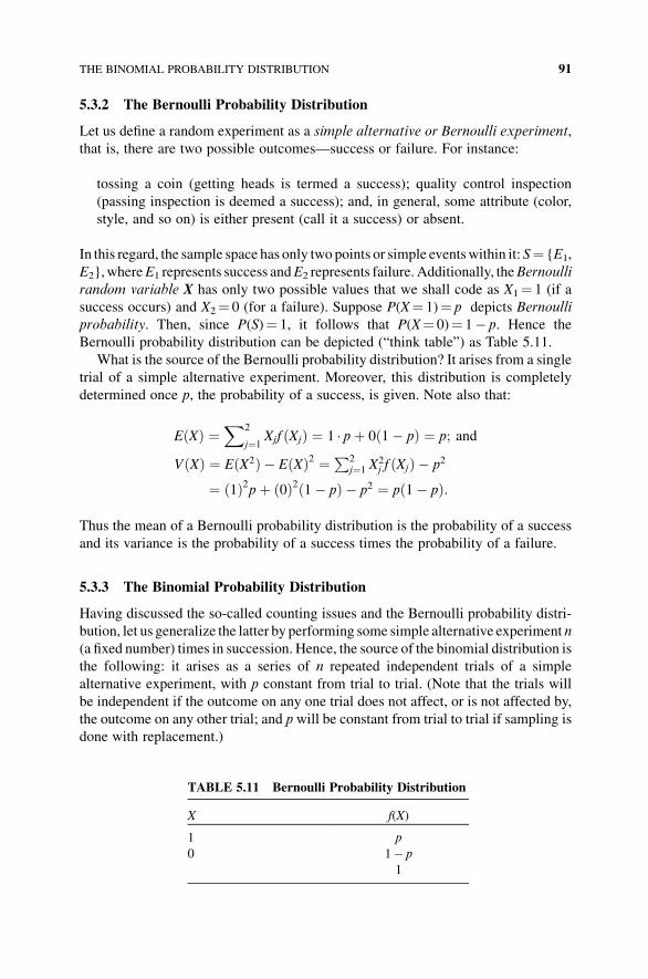
5.3.2 The Bernoulli Probability Distribution
Let us define a random experiment as a simple alternative or Bernoulli experiment,
that is, there are two possible outcomes—success or failure. For instance:
tossing a coin (getting heads is termed a success); quality control inspection
(passing inspection is deemed a success); and, in general, some attribute (color,
style, and so on) is either present (call it a success) or absent.
In this regard, the sample space has only two points or simple eventswithin it: S¼ {E1,
E2},whereE1 represents success andE2 represents failure. Additionally, theBernoulli
random variable X has only two possible values that we shall code as X1¼ 1 (if a
success occurs) and X2¼ 0 (for a failure). Suppose P(X¼ 1)¼ p depicts Bernoulli
probability. Then, since P(S)¼ 1, it follows that P(X¼ 0)¼ 1� p. Hence the
Bernoulli probability distribution can be depicted (“think table”) as Table 5.11.
What is the source of the Bernoulli probability distribution? It arises from a single
trial of a simple alternative experiment. Moreover, this distribution is completely
determined once p, the probability of a success, is given. Note also that:
EðXÞ ¼X2
j¼1Xjf ðXjÞ ¼ 1 � pþ 0ð1� pÞ ¼ p; and
VðXÞ ¼ EðX2Þ � EðXÞ2 ¼ P2j¼1 X
2j f ðXjÞ � p2
¼ ð1Þ2pþ ð0Þ2ð1� pÞ � p2 ¼ pð1� pÞ:
Thus the mean of a Bernoulli probability distribution is the probability of a success
and its variance is the probability of a success times the probability of a failure.
5.3.3 The Binomial Probability Distribution
Having discussed the so-called counting issues and the Bernoulli probability distri-
bution, let us generalize the latter by performing some simple alternative experiment n
(a fixed number) times in succession. Hence, the source of the binomial distribution is
the following: it arises as a series of n repeated independent trials of a simple
alternative experiment, with p constant from trial to trial. (Note that the trials will
be independent if the outcome on any one trial does not affect, or is not affected by,
the outcome on any other trial; and p will be constant from trial to trial if sampling is
done with replacement.)
TABLE 5.11 Bernoulli Probability Distribution
X f(X)
1 p
0 1� p
1
THE BINOMIAL PROBABILITY DISTRIBUTION 91
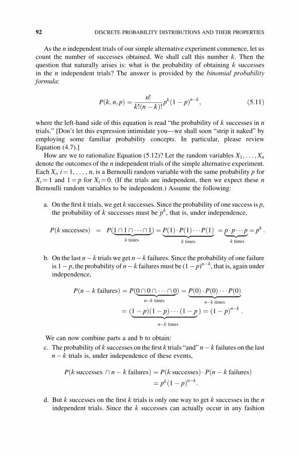
As the n independent trials of our simple alternative experiment commence, let us
count the number of successes obtained. We shall call this number k. Then the
question that naturally arises is: what is the probability of obtaining k successes
in the n independent trials? The answer is provided by the binomial probability
formula:
Pðk; n; pÞ ¼ n!
k!ðn� kÞ! pkð1� pÞn�k; ð5:11Þ
where the left-hand side of this equation is read “the probability of k successes in n
trials.” [Don’t let this expression intimidate you—we shall soon “strip it naked” by
employing some familiar probability concepts. In particular, please review
Equation (4.7).]
How are we to rationalize Equation (5.12)? Let the random variables X1; . . . ;Xn
denote the outcomes of the n independent trials of the simple alternative experiment.
Each Xi, i¼ 1, . . . , n, is a Bernoulli random variable with the same probability p for
Xi¼ 1 and 1¼ p for Xi¼ 0. (If the trials are independent, then we expect these n
Bernoulli random variables to be independent.) Assume the following:
a. On the first k trials, we get k successes. Since the probability of one success is p,
the probability of k successes must be pk, that is, under independence,
P k successesð Þ ¼ Pð1\ 1\ � � � \ 1|fflfflfflfflfflfflfflfflfflffl{zfflfflfflfflfflfflfflfflfflffl}Þk times
¼ Pð1Þ �Pð1Þ � � �Pð1Þ|fflfflfflfflfflfflfflfflfflfflfflfflfflffl{zfflfflfflfflfflfflfflfflfflfflfflfflfflffl}k times
¼ p �p � � �p|fflfflfflffl{zfflfflfflffl}¼ pk
k times
:
b. On the last n� k trials we get n� k failures. Since the probability of one failure
is 1� p, the probability of n� k failures must be (1� p)n�k, that is, again under
independence,
P n� k failuresð Þ ¼ Pð0 \ 0 \ � � � \ 0|fflfflfflfflfflfflfflfflfflffl{zfflfflfflfflfflfflfflfflfflffl}Þn�k times
¼ Pð0Þ �Pð0Þ � � �Pð0Þ|fflfflfflfflfflfflfflfflfflfflfflfflfflfflffl{zfflfflfflfflfflfflfflfflfflfflfflfflfflfflffl}n�k times
¼ ð1� pÞð1� pÞ � � � ð1� p|fflfflfflfflfflfflfflfflfflfflfflfflfflfflfflfflfflfflffl{zfflfflfflfflfflfflfflfflfflfflfflfflfflfflfflfflfflfflffl} Þ ¼ ð1� pÞn�k
n�k times
:
We can now combine parts a and b to obtain:
c. The probability of k successes on the first k trials “and” n� k failures on the last
n� k trials is, under independence of these events,
Pðk successes \ n� k failuresÞ ¼ Pðk successesÞ �Pðn� k failuresÞ¼ pkð1� pÞn�k:
d. But k successes on the first k trials is only one way to get k successes in the n
independent trials. Since the k successes can actually occur in any fashion
92 DISCRETE PROBABILITY DISTRIBUTIONS AND THEIR PROPERTIES
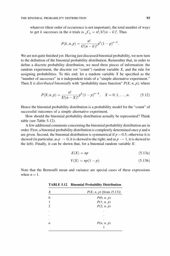
whatever (their order of occurrence is not important), the total number of ways
to get k successes in the n trials is nCk ¼ n!=k!ðn� kÞ!. Thus
Pðk; n; pÞ ¼ n!
k!ðn� kÞ! pkð1� pÞn�k:
Weare not quite finished yet. Having just discussed binomial probability, we now turn
to the definition of the binomial probability distribution. Remember that, in order to
define a discrete probability distribution, we need three pieces of information: the
random experiment, the discrete (or “count”) random variable X, and the rule for
assigning probabilities. To this end: let a random variable X be specified as the
“number of successes” in n independent trials of a “simple alternative experiment.”
Then X is distributed binomially with “probability mass function” P(X; n, p), where
PðX; n; pÞ ¼ n!
X!ðn� XÞ! pXð1� pÞn�X ; X ¼ 0; 1; . . . ; n: ð5:12Þ
Hence the binomial probability distribution is a probability model for the “count” of
successful outcomes of a simple alternative experiment.
How should the binomial probability distribution actually be represented? Think
table (see Table 5.12).
A few additional comments concerning the binomial probability distribution are in
order. First, a binomial probability distribution is completely determined once p and n
are given. Second, the binomial distribution is symmetrical if p¼ 0.5; otherwise it is
skewed (in particular, as p ! 0, it is skewed to the right; and as p ! 1, it is skewed to
the left). Finally, it can be shown that, for a binomial random variable X:
EðXÞ ¼ np ð5:13aÞVðXÞ ¼ npð1� pÞ: ð5:13bÞ
Note that the Bernoulli mean and variance are special cases of these expressions
when n¼ 1.
TABLE 5.12 Binomial Probability Distribution
X P(X; n, p) [from (5.13)]
0 P(0; n, p)
1 P(1; n, p)
2 P(2; n, p)
. .
. .
. .
n P(n; n, p)
1
THE BINOMIAL PROBABILITY DISTRIBUTION 93
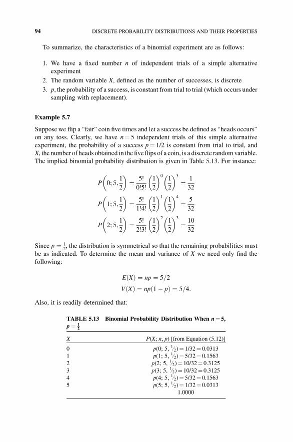
To summarize, the characteristics of a binomial experiment are as follows:
1. We have a fixed number n of independent trials of a simple alternative
experiment
2. The random variable X, defined as the number of successes, is discrete
3. p, the probability of a success, is constant from trial to trial (which occurs under
sampling with replacement).
Example 5.7
Suppose we flip a “fair” coin five times and let a success be defined as “heads occurs”
on any toss. Clearly, we have n¼ 5 independent trials of this simple alternative
experiment, the probability of a success p¼ 1/2 is constant from trial to trial, and
X, the number of heads obtained in the fiveflips of a coin, is a discrete randomvariable.
The implied binomial probability distribution is given in Table 5.13. For instance:
P 0; 5;1
2
� �¼ 5!
0!5!
1
2
� �01
2
� �5
¼ 1
32
P 1; 5;1
2
� �¼ 5!
1!4!
1
2
� �11
2
� �4
¼ 5
32
P 2; 5;1
2
� �¼ 5!
2!3!
1
2
� �21
2
� �3
¼ 10
32
Since p ¼ 12, the distribution is symmetrical so that the remaining probabilities must
be as indicated. To determine the mean and variance of X we need only find the
following:
EðXÞ ¼ np ¼ 5=2
VðXÞ ¼ npð1� pÞ ¼ 5=4:
Also, it is readily determined that:
TABLE 5.13 Binomial Probability Distribution When n¼ 5,
p ¼ 12
X P(X; n, p) [from Equation (5.12)]
0 p(0; 5, 1=2)¼ 1/32¼ 0.0313
1 p(1; 5, 1=2)¼ 5/32¼ 0.1563
2 p(2; 5, 1=2)¼ 10/32¼ 0.3125
3 p(3; 5, 1=2)¼ 10/32¼ 0.3125
4 p(4; 5, 1=2)¼ 5/32¼ 0.1563
5 p(5; 5, 1=2)¼ 1/32¼ 0.0313
1.0000
94 DISCRETE PROBABILITY DISTRIBUTIONS AND THEIR PROPERTIES
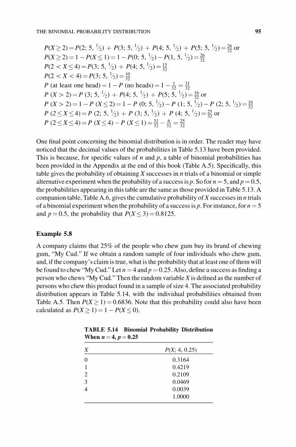
P(X� 2)¼P(2; 5, 1=2) þ P(3; 5, 1=2) þ P(4; 5, 1=2) þ P(5; 5, 1=2)¼ 2632
or
P(X� 2)¼ 1�P(X� 1)¼ 1�P(0; 5, 1=2)�P(1, 5, 1=2)¼ 2632
P(2GX� 4)¼P(3; 5, 1=2) þ P(4; 5, 1=2)¼ 1532
P(2GXG 4)¼P(3; 5, 1=2)¼ 1032
P (at least one head)¼ 1�P (no heads)¼ 1� 132¼ 31
32
P (XH 2)¼P (3; 5, 1=2) þ P(4; 5, 1=2) þ P(5; 5, 1=2)¼ 1632
or
P (XH 2)¼ 1�P (X� 2)¼ 1�P (0; 5, 1=2)�P (1; 5, 1=2)�P (2; 5, 1=2)¼ 1632
P (2�X� 4)¼P (2; 5, 1=2) þ P (3; 5, 1=2) þ P (4; 5, 1=2)¼ 2532
or
P (2�X� 4)¼P (X� 4)�P (X� 1)¼ 3132� 6
32¼ 25
32
One final point concerning the binomial distribution is in order. The reader may have
noticed that the decimal values of the probabilities in Table 5.13 have been provided.
This is because, for specific values of n and p, a table of binomial probabilities has
been provided in the Appendix at the end of this book (Table A.5). Specifically, this
table gives the probability of obtaining X successes in n trials of a binomial or simple
alternative experimentwhen the probability of a success is p. So for n¼ 5, and p¼ 0.5,
the probabilities appearing in this table are the same as those provided in Table 5.13. A
companion table, Table A.6, gives the cumulative probability ofX successes in n trials
of a binomial experimentwhen the probability of a success is p. For instance, for n¼ 5
and p¼ 0.5, the probability that P(X� 3)¼ 0.8125.
Example 5.8
A company claims that 25% of the people who chew gum buy its brand of chewing
gum, “My Cud.” If we obtain a random sample of four individuals who chew gum,
and, if the company’s claim is true, what is the probability that at least one of themwill
be found to chew “MyCud.” Let n¼ 4 and p¼ 0.25. Also, define a success as finding a
person who chews “MyCud.” Then the random variableX is defined as the number of
persons who chew this product found in a sample of size 4. The associated probability
distribution appears in Table 5.14, with the individual probabilities obtained from
Table A.5. Then P(X� 1)¼ 0.6836. Note that this probability could also have been
calculated as P(X� 1)¼ 1�P(X� 0).
TABLE 5.14 Binomial Probability Distribution
When n¼ 4, p¼ 0.25
X P(X; 4, 0.25)
0 0.3164
1 0.4219
2 0.2109
3 0.0469
4 0.0039
1.0000
THE BINOMIAL PROBABILITY DISTRIBUTION 95
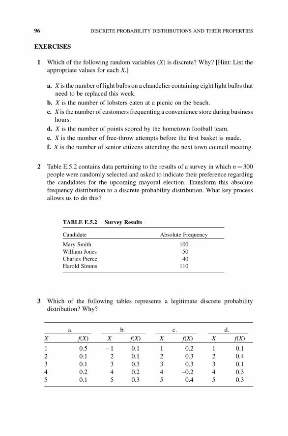
EXERCISES
1 Which of the following random variables (X) is discrete? Why? [Hint: List the
appropriate values for each X.]
a. X is the number of light bulbs on a chandelier containing eight light bulbs that
need to be replaced this week.
b. X is the number of lobsters eaten at a picnic on the beach.
c. X is the number of customers frequenting a convenience store during business
hours.
d. X is the number of points scored by the hometown football team.
e. X is the number of free-throw attempts before the first basket is made.
f. X is the number of senior citizens attending the next town council meeting.
2 Table E.5.2 contains data pertaining to the results of a survey in which n¼ 300
people were randomly selected and asked to indicate their preference regarding
the candidates for the upcoming mayoral election. Transform this absolute
frequency distribution to a discrete probability distribution. What key process
allows us to do this?
3 Which of the following tables represents a legitimate discrete probability
distribution? Why?
a. b. c. d.
X f(X) X f(X) X f(X) X f(X)
1 0.5 �1 0.1 1 0.2 1 0.1
2 0.1 2 0.1 2 0.3 2 0.4
3 0.1 3 0.3 3 0.3 3 0.1
4 0.2 4 0.2 4 –0.2 4 0.3
5 0.1 5 0.3 5 0.4 5 0.3
TABLE E.5.2 Survey Results
Candidate Absolute Frequency
Mary Smith 100
William Jones 50
Charles Pierce 40
Harold Simms 110
96 DISCRETE PROBABILITY DISTRIBUTIONS AND THEIR PROPERTIES
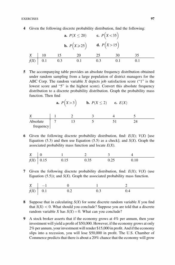
4 Given the following discrete probability distribution, find the following:
a. P X � 20ð Þ
b. P XX25� �
c. P XG35� �
d. P XH15� �
X 10 15 20 25 30 35
f(X) 0.1 0.3 0.1 0.3 0.1 0.1
5 The accompanying table provides an absolute frequency distribution obtained
under random sampling from a large population of district managers for the
ABC Corp. The random variable X depicts job satisfaction score (“1” is the
lowest score and “5” is the highest score). Convert this absolute frequency
distribution to a discrete probability distribution. Graph the probability mass
function. Then find
a. P XH3� �
b. P X � 2ð Þ c. E Xð Þ
X 1 2 3 4 5
Absolute
frequency
7 13 5 51 24
6 Given the following discrete probability distribution, find: E(X); V(X) [use
Equation (5.3) and then use Equation (5.5) as a check]; and S(X). Graph the
associated probability mass function and locate E(X).
X 0 1 2 3 4
f(X) 0.15 0.15 0.35 0.25 0.10
7 Given the following discrete probability distribution, find: E(X); V(X) (use
Equation (5.5)); and S(X). Graph the associated probability mass function.
X �1 0 1 2
f(X) 0.1 0.2 0.3 0.4
8 Suppose that in calculating S(X) for some discrete random variable X you find
that S(X)G 0. What should you conclude? Suppose you are told that a discrete
random variable X has S(X)¼ 0. What can you conclude?
9 A stock broker asserts that if the economy grows at 4% per annum, then your
investment will yield a profit of $50,000. However, if the economy grows at only
2%per annum, your investmentwill render $15,000 in profit.And if the economy
slips into a recession, you will lose $50,000 in profit. The U.S. Chamber of
Commerce predicts that there is about a 20% chance that the economy will grow
EXERCISES 97
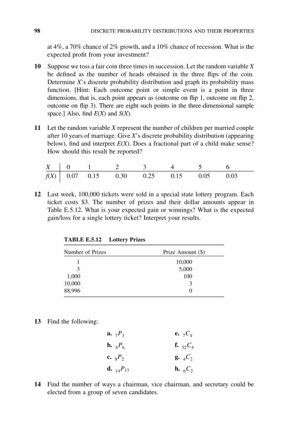
at 4%, a 70% chance of 2% growth, and a 10% chance of recession. What is the
expected profit from your investment?
10 Suppose we toss a fair coin three times in succession. Let the random variable X
be defined as the number of heads obtained in the three flips of the coin.
Determine X’s discrete probability distribution and graph its probability mass
function. [Hint: Each outcome point or simple event is a point in three
dimensions, that is, each point appears as (outcome on flip 1, outcome on flip 2,
outcome on flip 3). There are eight such points in the three-dimensional sample
space.] Also, find E(X) and S(X).
11 Let the random variable X represent the number of children per married couple
after 10 years of marriage. Give X’s discrete probability distribution (appearing
below), find and interpret E(X). Does a fractional part of a child make sense?
How should this result be reported?
X 0 1 2 3 4 5 6
f(X) 0.07 0.15 0.30 0.25 0.15 0.05 0.03
12 Last week, 100,000 tickets were sold in a special state lottery program. Each
ticket costs $3. The number of prizes and their dollar amounts appear in
Table E.5.12. What is your expected gain or winnings? What is the expected
gain/loss for a single lottery ticket? Interpret your results.
13 Find the following:
a. 7P3
b. 6P6
c. 8P2
d. 14P13
e. 7C4
f. 52C4
g. 4C2
h. 6C2
14 Find the number of ways a chairman, vice chairman, and secretary could be
elected from a group of seven candidates.
TABLE E.5.12 Lottery Prizes
Number of Prizes Prize Amount ($)
1 10,000
3 5,000
1,000 100
10,000 3
88,996 0
98 DISCRETE PROBABILITY DISTRIBUTIONS AND THEIR PROPERTIES
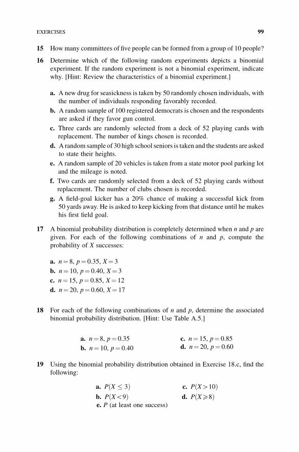
15 Howmany committees of five people can be formed from a group of 10 people?
16 Determine which of the following random experiments depicts a binomial
experiment. If the random experiment is not a binomial experiment, indicate
why. [Hint: Review the characteristics of a binomial experiment.]
a. A new drug for seasickness is taken by 50 randomly chosen individuals, with
the number of individuals responding favorably recorded.
b. A random sample of 100 registered democrats is chosen and the respondents
are asked if they favor gun control.
c. Three cards are randomly selected from a deck of 52 playing cards with
replacement. The number of kings chosen is recorded.
d. A random sample of 30 high school seniors is taken and the students are asked
to state their heights.
e. A random sample of 20 vehicles is taken from a state motor pool parking lot
and the mileage is noted.
f. Two cards are randomly selected from a deck of 52 playing cards without
replacement. The number of clubs chosen is recorded.
g. A field-goal kicker has a 20% chance of making a successful kick from
50 yards away. He is asked to keep kicking from that distance until he makes
his first field goal.
17 A binomial probability distribution is completely determined when n and p are
given. For each of the following combinations of n and p, compute the
probability of X successes:
a. n¼ 8, p¼ 0.35, X¼ 3
b. n¼ 10, p¼ 0.40, X¼ 3
c. n¼ 15, p¼ 0.85, X¼ 12
d. n¼ 20, p¼ 0.60, X¼ 17
18 For each of the following combinations of n and p, determine the associated
binomial probability distribution. [Hint: Use Table A.5.]
a. n¼ 8, p¼ 0.35
b. n¼ 10, p¼ 0.40
c. n¼ 15, p¼ 0.85
d. n¼ 20, p¼ 0.60
19 Using the binomial probability distribution obtained in Exercise 18.c, find the
following:
a. P X � 3ð Þb. PðXG9Þ
c. PðXH10Þd. PðXX8Þ
e. P (at least one success)
EXERCISES 99
20 For each of the binomial probability distributions obtained in Exercise 18, find
E(X) and V(X). [Hint: Use Equations (5.14a and b).]
21 According to a Washington, DC think tank, 55% of all Americans support some
form of so-called gun control. Suppose 12 citizens are randomly selected and
the number in favor of gun control is recorded. Find the following:
a. The probability that exactly seven of them are gun-control advocates.
b. The probability that at most eight of them favor gun control.
c. The probability that at least five of them favor gun control.
d. The probability that at least seven, but no more than 10, favor gun control.
22 In clinical trials of an experimental drug for the treatment of tree-nut allergies,
5% of the patients experienced a headache as a side effect. Suppose a random
sample of 20 subjects is taken and the number of them reporting a headache is
recorded. Find the following:
a. The probability that exactly three subjects experienced a headache as a side
effect.
b. The probability that no more than three subjects experienced a headache as a
side effect.
c. The probability that at least one, but nomore than four, subjects experienced a
headache as a side effect.
d. The probability that at least half of the subjects experienced a headache as a
side effect.
100 DISCRETE PROBABILITY DISTRIBUTIONS AND THEIR PROPERTIES
6THE NORMAL DISTRIBUTION
6.1 THE CONTINUOUS PROBABILITY DISTRIBUTION
A probability distribution is termed continuous if its underlying random variable X is
continuous, that is, if X can assume an infinite or uncountable number of real values
over some interval. Such variables are “measured” in terms of distance, temperature,
weight, time, and so on. For instance, X¼ time between arrivals of vehicles at a toll
booth is a continuous random variable. Also, if two points A and B are chosen at
randomon a real line segment of lengthL (Fig. 6.1), then the distanceX ¼ A� Bj j (theabsolute value1 of A minus B), 0 � X � L; can assume an infinite number of values
and thus is a continuous random variable. [How about this definition of a continuous
random variable? A random variable X is continuous if PðX ¼ aÞ ¼ 0 for all real a.
Does it work?]
The expression representing a continuous random variable X is called a prob-
ability density function. With X being continuous, its probability density function
can be drawn without lifting one’s pen from a sheet of paper. Hence the graph of X’s
probability density function is without breaks. More formally, a real-valued
function f is a probability density function for a continuous random variable X
if (a) f ðxÞ � 0 for all real x 2 ð�1;þ1Þ and (b) the total area beneath f ðxÞ is one.
Statistical Inference: A Short Course, First Edition. Michael J. Panik.� 2012 John Wiley & Sons, Inc. Published 2012 by John Wiley & Sons, Inc.
1 The absolute value function is defined as follows:
xj j ¼ x; x � 0
�x; xG0
�
101
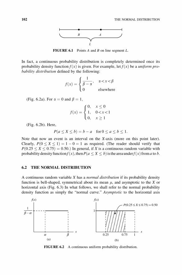
In fact, a continuous probability distribution is completely determined once its
probability density function f ðxÞ is given. For example, let f ðxÞ be a uniform pro-
bability distribution defined by the following:
f ðxÞ ¼1
b� a; aGxGb
0 elsewhere
8<
:
(Fig. 6.2a). For a ¼ 0 and b ¼ 1;
f ðxÞ ¼0; x � 0
1; 0GxG1
0; x � 1
8<
:
(Fig. 6.2b). Here,
Pða � X � bÞ ¼ b� a for 0 � a � b � 1:
Note that now an event is an interval on the X-axis (more on this point later).
Clearly, Pð0 � X � 1Þ ¼ 1� 0 ¼ 1 as required. (The reader should verify that
Pð0:25 � X � 0:75Þ ¼ 0:50:Þ In general, if X is a continuous random variable with
probabilitydensity function f ðxÞ, thenPða � X � bÞ is theareaunder f ðxÞ froma to b.
6.2 THE NORMAL DISTRIBUTION
A continuous random variable X has a normal distribution if its probability density
function is bell-shaped, symmetrical about its mean m, and asymptotic to the X or
horizontal axis (Fig. 6.3) In what follows, we shall refer to the normal probability
density function as simply the “normal curve.” Asymptotic to the horizontal axis
• •
L
B A
FIGURE 6.1 Points A and B on line segment L:
(a) (b)
α
β − α
βx x
f(x) f(x)
P(0.25 ≤ X ≤ 0.75) = 0.501
0.25 0.75 1
1
FIGURE 6.2 A continuous uniform probability distribution.
102 THE NORMAL DISTRIBUTION
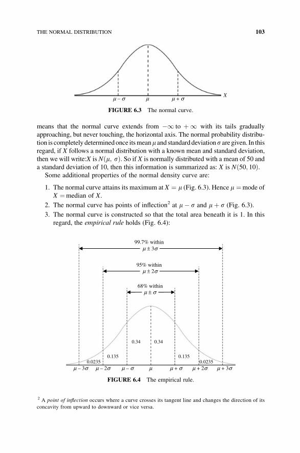
means that the normal curve extends from �1 to þ1 with its tails gradually
approaching, but never touching, the horizontal axis. The normal probability distribu-
tion is completely determinedonce itsmeanm and standarddeviations aregiven. In thisregard, if X follows a normal distribution with a known mean and standard deviation,
then we will write:X is Nðm; sÞ. So if X is normally distributed with a mean of 50 and
a standard deviation of 10, then this information is summarized as: X is Nð50; 10Þ.Some additional properties of the normal density curve are:
1. The normal curve attains its maximum at X ¼ m (Fig. 6.3). Hence m ¼mode of
X ¼median of X.
2. The normal curve has points of inflection2 at m� s and mþ s (Fig. 6.3).
3. The normal curve is constructed so that the total area beneath it is 1. In this
regard, the empirical rule holds (Fig. 6.4):
Xμ + σμ – σ μ
FIGURE 6.3 The normal curve.
68% within
95% within
99.7% withinμ ± 3σ
μ + 3σμ + 2σμ + σμ – 3σ μ – 2σ μ – σ μ
μ ± 2σ
μ ± σ
0.34 0.34
0.135 0.1350.0235 0.0235
FIGURE 6.4 The empirical rule.
2 A point of inflection occurs where a curve crosses its tangent line and changes the direction of its
concavity from upward to downward or vice versa.
THE NORMAL DISTRIBUTION 103
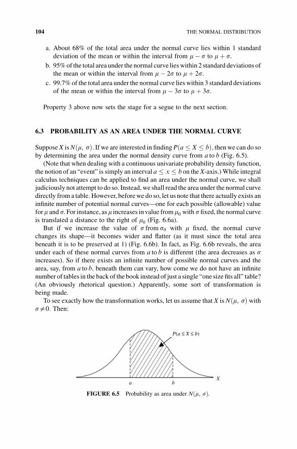
a. About 68% of the total area under the normal curve lies within 1 standard
deviation of the mean or within the interval from m� s to mþ s.b. 95%of the total area under the normal curve lieswithin 2 standard deviations of
the mean or within the interval from m� 2s to mþ 2s.c. 99.7%of the total area under the normal curve lies within 3 standard deviations
of the mean or within the interval from m� 3s to mþ 3s.
Property 3 above now sets the stage for a segue to the next section.
6.3 PROBABILITY AS AN AREA UNDER THE NORMAL CURVE
SupposeX isNðm; sÞ: If we are interested in findingPða � X � bÞ; then we can do soby determining the area under the normal density curve from a to b (Fig. 6.5).
(Note that when dealing with a continuous univariate probability density function,
the notion of an “event” is simply an interval a � x � b on theX-axis.)While integral
calculus techniques can be applied to find an area under the normal curve, we shall
judiciously not attempt to do so. Instead,we shall read the area under the normal curve
directly from a table. However, beforewe do so, let us note that there actually exists an
infinite number of potential normal curves—one for each possible (allowable) value
form and s. For instance, asm increases invalue fromm0 with sfixed, the normal curve
is translated a distance to the right of m0 (Fig. 6.6a).But if we increase the value of s from s0 with m fixed, the normal curve
changes its shape—it becomes wider and flatter (as it must since the total area
beneath it is to be preserved at 1) (Fig. 6.6b). In fact, as Fig. 6.6b reveals, the area
under each of these normal curves from a to b is different (the area decreases as sincreases). So if there exists an infinite number of possible normal curves and the
area, say, from a to b; beneath them can vary, how come we do not have an infinite
number of tables in the back of the book instead of just a single “one size fits all” table?
(An obviously rhetorical question.) Apparently, some sort of transformation is
being made.
To see exactly how the transformation works, let us assume that X is Nðm; sÞwiths$0: Then:
a b
P(a ≤ X ≤ b)
X
FIGURE 6.5 Probability as area under Nðm; sÞ.
104 THE NORMAL DISTRIBUTION
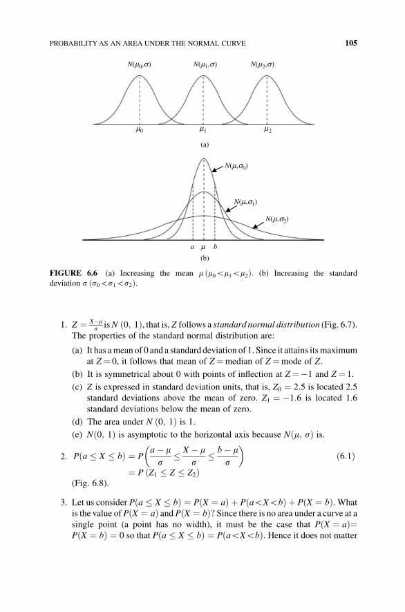
1. Z ¼ X�ms isN ð0; 1Þ, that is, Z follows a standard normal distribution (Fig. 6.7).
The properties of the standard normal distribution are:
(a) It has amean of 0 and a standard deviation of 1. Since it attains itsmaximum
at Z ¼ 0, it follows that mean of Z¼median of Z¼mode of Z.
(b) It is symmetrical about 0 with points of inflection at Z¼�1 and Z¼ 1.
(c) Z is expressed in standard deviation units, that is, Z0 ¼ 2:5 is located 2.5
standard deviations above the mean of zero. Z1 ¼ �1:6 is located 1.6
standard deviations below the mean of zero.
(d) The area under N ð0; 1Þ is 1.(e) Nð0; 1Þ is asymptotic to the horizontal axis because Nðm; sÞ is.
2. Pða � X � bÞ ¼ Pa� ms
� X � ms
� b� ms
� �ð6:1Þ
¼ P ðZ1 � Z � Z2Þ(Fig. 6.8).
3. Let us consider Pða � X � bÞ ¼ PðX ¼ aÞ þ PðaGXGbÞ þ PðX ¼ bÞ:What
is the value ofPðX ¼ aÞ and PðX ¼ bÞ? Since there is no area under a curve at asingle point (a point has no width), it must be the case that PðX ¼ aÞ¼PðX ¼ bÞ ¼ 0 so that Pða � X � bÞ ¼ PðaGXGbÞ: Hence it does not matter
N(μ0,σ) N(μ1,σ)
N(μ,σ1)
N(μ,σ0)
N(μ,σ2)
N(μ2,σ)
(a)
(b)
a b
μ0 μ1
μ
μ2
FIGURE 6.6 (a) Increasing the mean m ðm0Gm1Gm2Þ: (b) Increasing the standard
deviation s ðs0Gs1Gs2Þ.
PROBABILITYAS AN AREA UNDER THE NORMAL CURVE 105
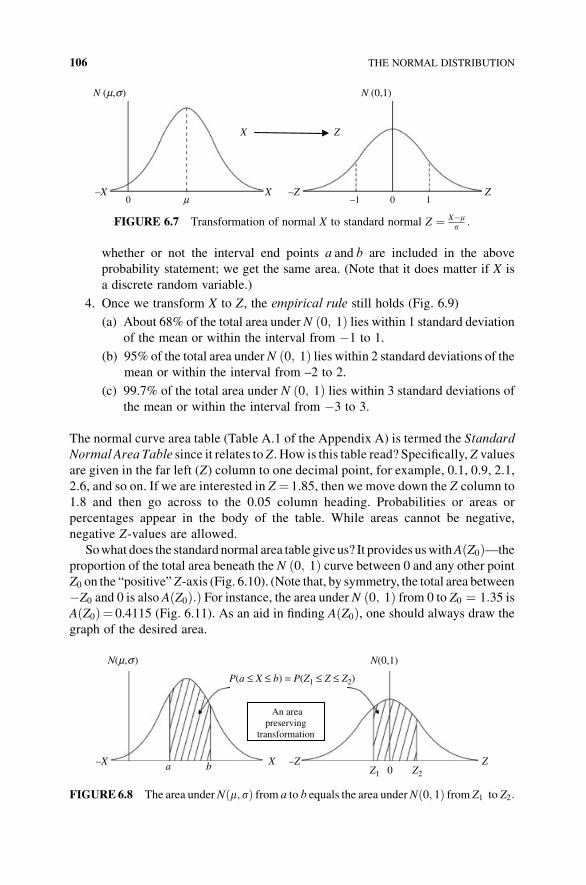
whether or not the interval end points a and b are included in the above
probability statement; we get the same area. (Note that it does matter if X is
a discrete random variable.)
4. Once we transform X to Z, the empirical rule still holds (Fig. 6.9)
(a) About 68% of the total area under N ð0; 1Þ lies within 1 standard deviationof the mean or within the interval from �1 to 1.
(b) 95% of the total area underN ð0; 1Þ lies within 2 standard deviations of themean or within the interval from –2 to 2.
(c) 99.7% of the total area under N ð0; 1Þ lies within 3 standard deviations of
the mean or within the interval from �3 to 3.
The normal curve area table (Table A.1 of the Appendix A) is termed the Standard
Normal Area Table since it relates to Z. How is this table read? Specifically, Z values
are given in the far left (Z) column to one decimal point, for example, 0.1, 0.9, 2.1,
2.6, and so on. If we are interested in Z ¼ 1.85, then we move down the Z column to
1.8 and then go across to the 0.05 column heading. Probabilities or areas or
percentages appear in the body of the table. While areas cannot be negative,
negative Z-values are allowed.
Sowhat does the standard normal area table give us? It provides uswithAðZ0Þ—the
proportion of the total area beneath the N ð0; 1Þ curve between 0 and any other pointZ0 on the “positive”Z-axis (Fig. 6.10). (Note that, by symmetry, the total area between
�Z0 and 0 is also AðZ0Þ:Þ For instance, the area under N ð0; 1Þ from 0 to Z0 ¼ 1:35 isAðZ0Þ¼ 0.4115 (Fig. 6.11). As an aid in finding AðZ0Þ, one should always draw the
graph of the desired area.
X
–X –Z ZX
Z
N (μ,σ) N (0,1)
0 –1 10μ
FIGURE 6.7 Transformation of normal X to standard normal Z ¼ X�ms :
P(a ≤ X ≤ b) = P(Z1 ≤ Z ≤ Z2)
0Z1 Z2
–X –Z ZXa b
N(μ,σ ) N(0,1)
An area preserving
transformation
FIGURE6.8 The area underNðm; sÞ from a to b equals the area underNð0; 1Þ from Z1 to Z2:
106 THE NORMAL DISTRIBUTION
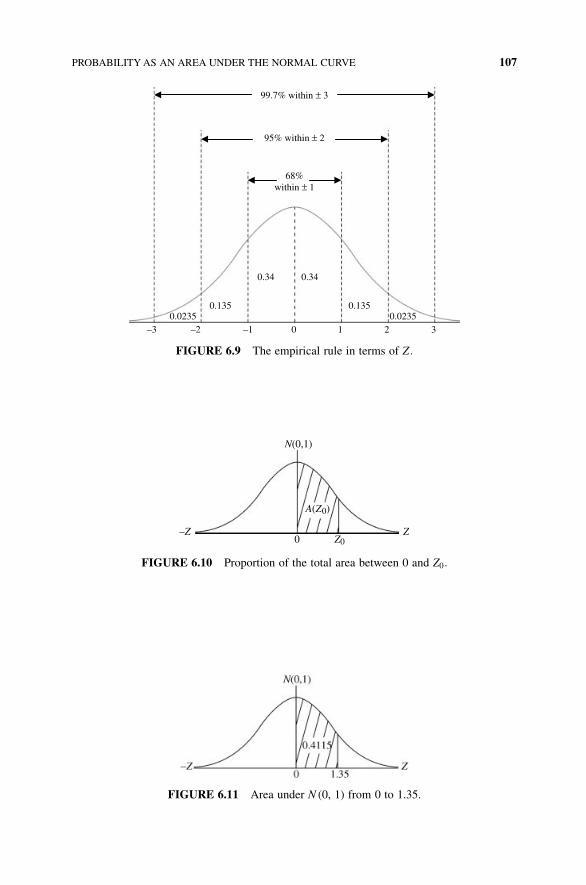
0–1–2–3 321
68%within ± 1
95% within ± 2
99.7% within ± 3
0.34 0.34
0.135 0.1350.0235 0.0235
FIGURE 6.9 The empirical rule in terms of Z:
N(0,1)
A(Z0)
0 Z0–Z Z
FIGURE 6.10 Proportion of the total area between 0 and Z0:
FIGURE 6.11 Area under N (0, 1) from 0 to 1.35.
PROBABILITYAS AN AREA UNDER THE NORMAL CURVE 107
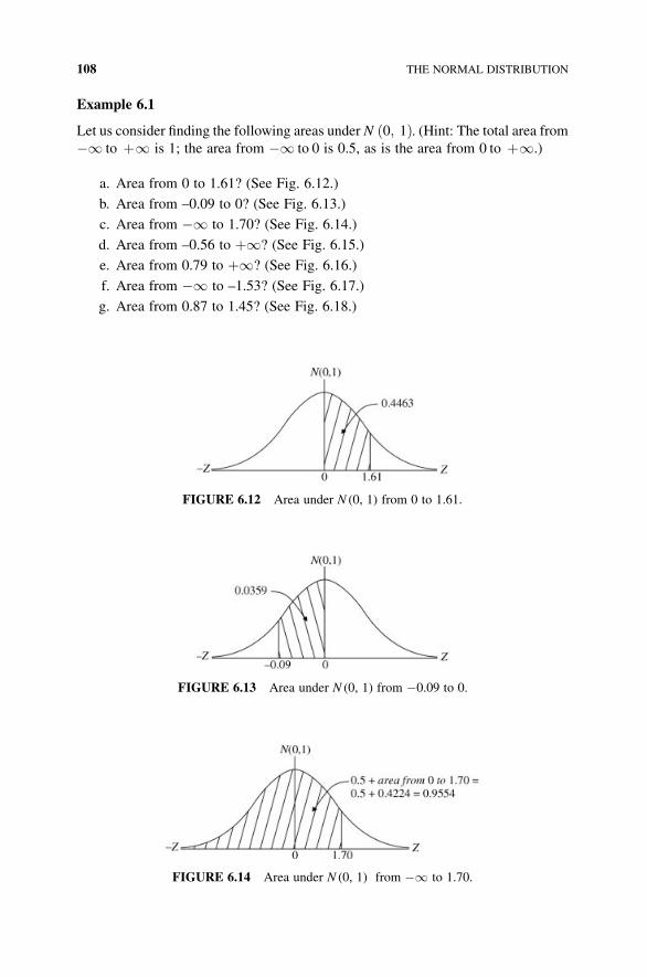
Example 6.1
Let us consider finding the following areas under N ð0; 1Þ. (Hint: The total area from�1 to þ1 is 1; the area from �1 to 0 is 0.5, as is the area from 0 to þ1.)
a. Area from 0 to 1.61? (See Fig. 6.12.)
b. Area from –0.09 to 0? (See Fig. 6.13.)
c. Area from �1 to 1.70? (See Fig. 6.14.)
d. Area from –0.56 to þ1? (See Fig. 6.15.)
e. Area from 0.79 to þ1? (See Fig. 6.16.)
f. Area from �1 to –1.53? (See Fig. 6.17.)
g. Area from 0.87 to 1.45? (See Fig. 6.18.)
FIGURE 6.12 Area under N (0, 1) from 0 to 1.61.
FIGURE 6.13 Area under N (0, 1) from �0.09 to 0.
FIGURE 6.14 Area under N (0, 1) from �1 to 1.70.
108 THE NORMAL DISTRIBUTION
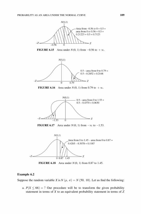
Example 6.2
Suppose the random variable X isN ðm; sÞ ¼ N ð50; 10Þ: Let us find the following:
a. PðX � 66Þ ¼ ? Our procedure will be to transform the given probability
statement in terms of X to an equivalent probability statement in terms of Z
FIGURE 6.15 Area under N (0, 1) from �0.56 to þ1.
FIGURE 6.16 Area under N (0, 1) from 0.79 to þ1.
FIGURE 6.17 Area under N (0, 1) from �1 to �1.53.
FIGURE 6.18 Area under N (0, 1) from 0.87 to 1.45.
PROBABILITYAS AN AREA UNDER THE NORMAL CURVE 109
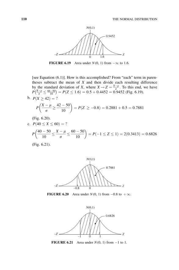
[see Equation (6.1)]. How is this accomplished? From “each” term in paren-
theses subtract the mean of X and then divide each resulting difference
by the standard deviation of X, where X! Z ¼ X�ms : To this end, we have
P X�ms � 66�50
10
� � ¼ PðZ � 1:6Þ ¼ 0:5þ 0:4452 ¼ 0:9452 (Fig. 6.19).
b. PðX � 42Þ ¼ ?
PX � ms
� 42� 50
10
� �¼ PðZ � �0:8Þ ¼ 0:2881þ 0:5 ¼ 0:7881
(Fig. 6.20).
c. Pð40 � X � 60Þ ¼ ?
P40� 50
10� X � m
s� 60� 50
10
� �¼ Pð�1 � Z � 1Þ ¼ 2ð0:3413Þ ¼ 0:6826
(Fig. 6.21).
FIGURE 6.19 Area under N (0, 1) from �1 to 1.6.
FIGURE 6.20 Area under N (0, 1) from �0.8 to þ1.
FIGURE 6.21 Area under N (0, 1) from �1 to 1.
110 THE NORMAL DISTRIBUTION
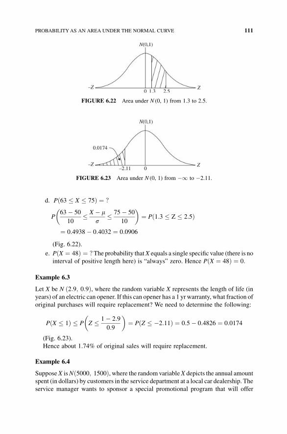
d. Pð63 � X � 75Þ ¼ ?
P63� 50
10� X � m
s� 75� 50
10
� �¼ Pð1:3 � Z � 2:5Þ
¼ 0:4938� 0:4032 ¼ 0:0906
(Fig. 6.22).
e. PðX ¼ 48Þ ¼ ?The probability thatX equals a single specific value (there is no
interval of positive length here) is “always” zero. Hence PðX ¼ 48Þ ¼ 0:
Example 6.3
Let X be N ð2:9; 0:9Þ, where the random variable X represents the length of life (in
years) of an electric can opener. If this can opener has a 1 yr warranty, what fraction of
original purchases will require replacement? We need to determine the following:
PðX � 1Þ � P
�Z � 1� 2:9
0:9
�¼ PðZ � �2:11Þ ¼ 0:5� 0:4826 ¼ 0:0174
(Fig. 6.23).
Hence about 1.74% of original sales will require replacement.
Example 6.4
SupposeX isNð5000; 1500Þ, where the random variableX depicts the annual amount
spent (in dollars) by customers in the service department at a local car dealership. The
service manager wants to sponsor a special promotional program that will offer
FIGURE 6.22 Area under N (0, 1) from 1.3 to 2.5.
FIGURE 6.23 Area under N (0, 1) from �1 to �2.11.
PROBABILITYAS AN AREA UNDER THE NORMAL CURVE 111
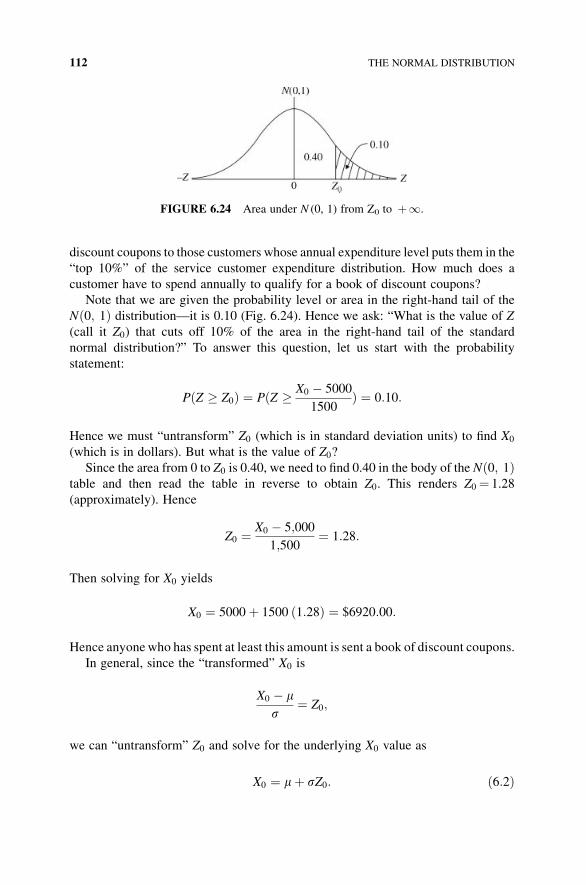
discount coupons to those customers whose annual expenditure level puts them in the
“top 10%” of the service customer expenditure distribution. How much does a
customer have to spend annually to qualify for a book of discount coupons?
Note that we are given the probability level or area in the right-hand tail of the
Nð0; 1Þ distribution—it is 0.10 (Fig. 6.24). Hence we ask: “What is the value of Z
(call it Z0) that cuts off 10% of the area in the right-hand tail of the standard
normal distribution?” To answer this question, let us start with the probability
statement:
PðZ � Z0Þ ¼ PðZ � X0 � 5000
1500Þ ¼ 0:10:
Hence we must “untransform” Z0 (which is in standard deviation units) to find X0
(which is in dollars). But what is the value of Z0?
Since the area from 0 to Z0 is 0.40, we need to find 0.40 in the body of the Nð0; 1Þtable and then read the table in reverse to obtain Z0. This renders Z0 ¼ 1.28
(approximately). Hence
Z0 ¼ X0 � 5;000
1;500¼ 1:28:
Then solving for X0 yields
X0 ¼ 5000þ 1500 ð1:28Þ ¼ $6920:00:
Hence anyonewho has spent at least this amount is sent a book of discount coupons.
In general, since the “transformed” X0 is
X0 � ms
¼ Z0;
we can “untransform” Z0 and solve for the underlying X0 value as
X0 ¼ mþ sZ0: ð6:2Þ
FIGURE 6.24 Area under N (0, 1) from Z0 to þ1.
112 THE NORMAL DISTRIBUTION
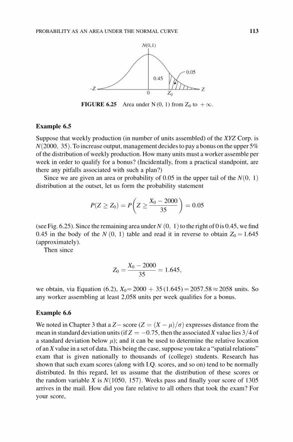
Example 6.5
Suppose that weekly production (in number of units assembled) of the XYZ Corp. is
Nð2000; 35Þ. To increase output,management decides to pay a bonus on the upper 5%
of the distribution of weekly production. Howmany units must aworker assemble per
week in order to qualify for a bonus? (Incidentally, from a practical standpoint, are
there any pitfalls associated with such a plan?)
Since we are given an area or probability of 0.05 in the upper tail of the Nð0; 1Þdistribution at the outset, let us form the probability statement
PðZ � Z0Þ ¼ P
�Z � X0 � 2000
35
�¼ 0:05
(see Fig. 6.25). Since the remaining area underN ð0; 1Þ to the right of 0 is 0.45,wefind0.45 in the body of the N ð0; 1Þ table and read it in reverse to obtain Z0 ¼ 1.645
(approximately).
Then since
Z0 ¼ X0 � 2000
35¼ 1:645;
we obtain, via Equation (6.2), X0¼ 2000 þ 35 (1.645)¼ 2057.58� 2058 units. So
any worker assembling at least 2,058 units per week qualifies for a bonus.
Example 6.6
We noted in Chapter 3 that a Z� score (Z ¼ ðX � mÞ=sÞ expresses distance from the
mean in standard deviation units (ifZ ¼ �0:75; then the associatedX value lies 3=4 ofa standard deviation below m); and it can be used to determine the relative location
of anX value in a set of data. This being the case, suppose you take a “spatial relations”
exam that is given nationally to thousands of (college) students. Research has
shown that such exam scores (along with I.Q. scores, and so on) tend to be normally
distributed. In this regard, let us assume that the distribution of these scores or
the random variable X is Nð1050; 157Þ: Weeks pass and finally your score of 1305
arrives in the mail. How did you fare relative to all others that took the exam? For
your score,
FIGURE 6.25 Area under N (0, 1) from Z0 to þ1.
PROBABILITYAS AN AREA UNDER THE NORMAL CURVE 113
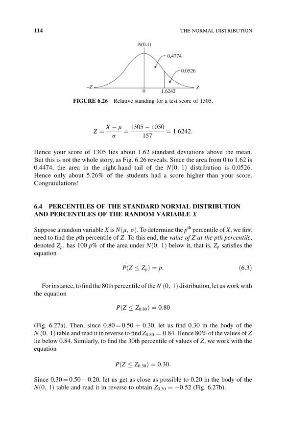
Z ¼ X � ms
¼ 1305� 1050
157¼ 1:6242:
Hence your score of 1305 lies about 1.62 standard deviations above the mean.
But this is not the whole story, as Fig. 6.26 reveals. Since the area from 0 to 1.62 is
0.4474, the area in the right-hand tail of the Nð0; 1Þ distribution is 0.0526.
Hence only about 5.26% of the students had a score higher than your score.
Congratulations!
6.4 PERCENTILES OF THE STANDARD NORMAL DISTRIBUTION
AND PERCENTILES OF THE RANDOM VARIABLE X
Suppose a random variable X isNðm; sÞ. To determine the pth percentile of X, we first
need to find the pth percentile of Z: To this end, the value of Z at the pth percentile,
denoted Zp; has 100 p% of the area under Nð0; 1Þ below it, that is, Zp satisfies the
equation
PðZ � ZpÞ ¼ p: ð6:3Þ
For instance, to find the 80th percentile of theN ð0; 1Þ distribution, let usworkwiththe equation
PðZ � Z0:80Þ ¼ 0:80
(Fig. 6.27a). Then, since 0.80¼ 0.50 þ 0.30, let us find 0.30 in the body of the
N ð0; 1Þ table and read it in reverse to find Z0:80 ¼ 0:84. Hence 80% of the values of Z
lie below 0.84. Similarly, to find the 30th percentile of values of Z, we work with the
equation
PðZ � Z0:30Þ ¼ 0:30:
Since 0.30¼ 0.50� 0.20, let us get as close as possible to 0.20 in the body of the
Nð0; 1Þ table and read it in reverse to obtain Z0:30 ¼ �0:52 (Fig. 6.27b).
FIGURE 6.26 Relative standing for a test score of 1305.
114 THE NORMAL DISTRIBUTION
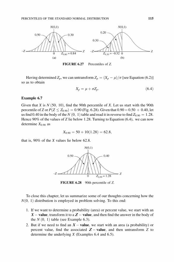
Having determined Zp, we can untransform Zp ¼ ðXp � mÞ=s [see Equation (6.2)]
so as to obtain
Xp ¼ mþ sZp: ð6:4Þ
Example 6.7
Given that X is N ð50; 10Þ, find the 90th percentile of X. Let us start with the 90th
percentile of Z orPðZ � Z0:90Þ ¼ 0:90 (Fig. 6.28). Given that 0.90¼ 0.50 þ 0.40, let
us find 0.40 in the body of theN ð0; 1Þ table and read it in reverse to find Z0:90 ¼ 1:28:Hence 90% of the values of Z lie below 1.28. Turning to Equation (6.4), we can now
determine X0:90 as
X0:90 ¼ 50þ 10ð1:28Þ ¼ 62:8;
that is, 90% of the X values lie below 62.8.
To close this chapter, let us summarize some of our thoughts concerning how the
Nð0; 1Þ distribution is employed in problem solving. To this end:
1. If we want to determine a probability (area) or percent value, we start with an
X� value; transform it to aZ� value; and then find the answer in the body ofthe N ð0; 1Þ table (see Example 6.3).
2. But if we need to find an X� value; we start with an area (a probability) or
percent value, find the associated Z� value; and then untransform Z to
determine the underlying X (Examples 6.4 and 6.5).
FIGURE 6.28 90th percentile of Z.
FIGURE 6.27 Percentiles of Z.
PERCENTILES OF THE STANDARD NORMAL DISTRIBUTION 115
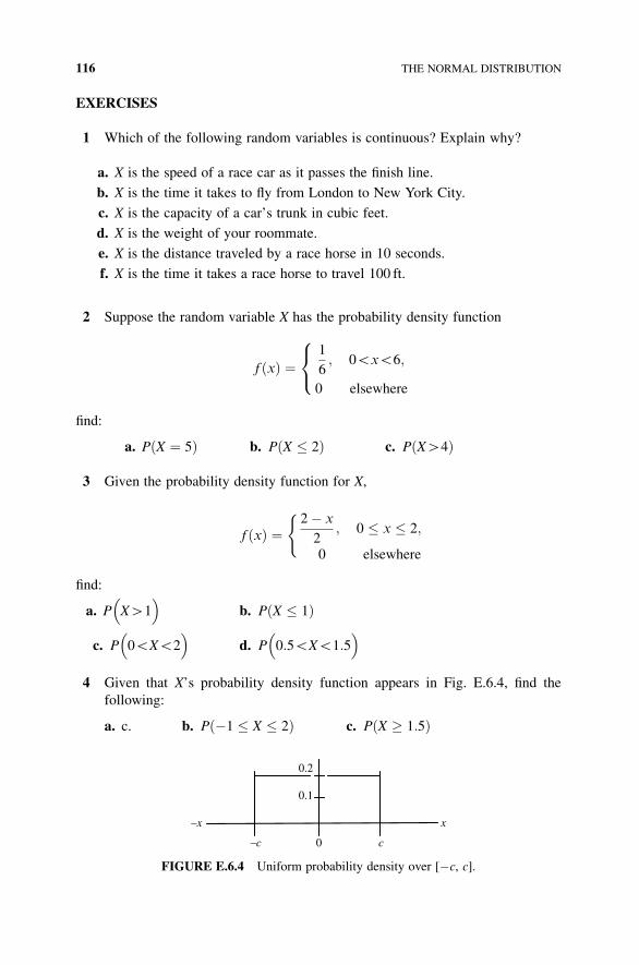
EXERCISES
1 Which of the following random variables is continuous? Explain why?
a. X is the speed of a race car as it passes the finish line.
b. X is the time it takes to fly from London to New York City.
c. X is the capacity of a car’s trunk in cubic feet.
d. X is the weight of your roommate.
e. X is the distance traveled by a race horse in 10 seconds.
f. X is the time it takes a race horse to travel 100 ft.
2 Suppose the random variable X has the probability density function
f ðxÞ ¼1
6; 0GxG6;
0 elsewhere
8<
:
find:
a. P X ¼ 5ð Þ b. P X � 2ð Þ c. PðXH4Þ
3 Given the probability density function for X,
f ðxÞ ¼2� x
2; 0 � x � 2;
0 elsewhere
(
find:
a. P XH1� �
b. P X � 1ð Þ
c. P 0GXG2� �
d. P 0:5GXG1:5� �
4 Given that X’s probability density function appears in Fig. E.6.4, find the
following:
a. c. b. P �1 � X � 2ð Þ c. P X � 1:5ð Þ
0.2
0.1
–x x
–c 0 c
FIGURE E.6.4 Uniform probability density over [�c, c].
116 THE NORMAL DISTRIBUTION
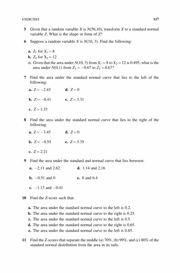
5 Given that a random variable X is N(50,10), transform X to a standard normal
variable Z. What is the shape or form of Z?
6 Suppose a random variable X is N(10, 3). Find the following:
a. Z1 for X1¼ 8
b. Z2 for X2¼ 12
c. Given that the area under N(10, 3) from X1¼ 8 to X2¼ 12 is 0.495, what is the
area under N(0,1) from Z1¼�0.67 to Z2¼ 0.67?
7 Find the area under the standard normal curve that lies to the left of the
following:
a. Z¼�2.43 d. Z¼ 0
b. Z¼�0.41
c. Z¼ 1.33
e. Z¼ 3.31
8 Find the area under the standard normal curve that lies to the right of the
following:
a. Z¼�3.45 d. Z¼ 0
b. Z¼�0.55
c. Z¼ 2.21
e. Z¼ 3.35
9 Find the area under the standard and normal curve that lies between:
a. �2.11 and 2.62 d. 1.14 and 2.16
b. �0.51 and 0
c. �1.13 and �0.41
e. 0 and 6.4
10 Find the Z-score such that:
a. The area under the standard normal curve to the left is 0.2.
b. The area under the standard normal curve to the right is 0.25.
c. The area under the standard normal curve to the left is 0.5.
d. The area under the standard normal curve to the right is 0.65.
e. The area under the standard normal curve to the left is 0.85.
11 Find the Z-scores that separate the middle (a) 70%, (b) 99%, and (c) 80% of the
standard normal distribution from the area in its tails.
EXERCISES 117
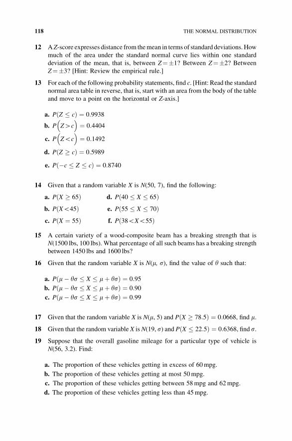
12 AZ-score expresses distance from themean in terms of standard deviations. How
much of the area under the standard normal curve lies within one standard
deviation of the mean, that is, between Z¼�1? Between Z¼�2? Between
Z¼�3? [Hint: Review the empirical rule.]
13 For each of the following probability statements, find c. [Hint: Read the standard
normal area table in reverse, that is, start with an area from the body of the table
and move to a point on the horizontal or Z-axis.]
a. P Z � cð Þ ¼ 0:9938
b. P ZHc� �
¼ 0:4404
c. P ZGc� �
¼ 0:1492
d. P Z � cð Þ ¼ 0:5989
e. P �c � Z � cð Þ ¼ 0:8740
14 Given that a random variable X is N(50, 7), find the following:
a. P X � 65ð Þb. PðXG45Þc. P X ¼ 55ð Þ
d. P 40 � X � 65ð Þe. P 55 � X � 70ð Þf. Pð38GXG55Þ
15 A certain variety of a wood-composite beam has a breaking strength that is
N(1500 lbs, 100 lbs). What percentage of all such beams has a breaking strength
between 1450 lbs and 1600 lbs?
16 Given that the random variable X is N(m, s), find the value of y such that:
a. P m� ys � X � mþ ysð Þ ¼ 0:95
b. P m� ys � X � mþ ysð Þ ¼ 0:90
c. P m� ys � X � mþ ysð Þ ¼ 0:99
17 Given that the random variable X is N(m, 5) and P X � 78:5ð Þ ¼ 0:0668, find m.
18 Given that the random variable X is N(19, s) and P X � 22:5ð Þ ¼ 0:6368, find s.
19 Suppose that the overall gasoline mileage for a particular type of vehicle is
N(56, 3.2). Find:
a. The proportion of these vehicles getting in excess of 60mpg.
b. The proportion of these vehicles getting at most 50mpg.
c. The proportion of these vehicles getting between 58mpg and 62mpg.
d. The proportion of these vehicles getting less than 45mpg.
118 THE NORMAL DISTRIBUTION

20 A random variable X is N(30, 8). Find the indicated percentile for X:
a. The 10th percentile
b. The 90th percentile
c. The 80th percentile
d. The 50th percentile
21 The research arm of theABCCorp. has determined that the use time (in hours) of
its microbattery is N(324, 24). Find:
a. The proportion of time that the microbattery will last at least 300 hours.
b. The proportion of time it will last between 310 hr and 350 hr.
c. The use time that is in the top 20% of the distribution.
d. The range of use time that constitutes the middle 90% of the distribution.
22 The average stock price for companies constituting the Standard & Poor’s
(S&P) 500 Index is $30 and the standard deviation of the stock prices is $8.20. If
the implied distribution of stock prices is assumed to be normal, find the
following:
a. The probability that an S&P 500 company will have a stock price not higher
than $20.
b. The probability that an S&P 500 company will have a stock price of at least $40.
c. How high does a stock price have to be in order to put an S&P 500 company in
the top 10% of the distribution of S&P 500 stock prices?
d. The range of stock prices that make up the middle 80% of the distribution of
S&P 500 stock prices.
23 A college basketball player must have a points-per-game average in the upper
2% of all college basketball players in order to qualify forAll American status. If
points-per-game values are normally distributed with a mean of 25 and a
standard deviation of 15, what points-per-game average must a player have
in order to qualify for All American?
24 For a large group of trade school applicants the distribution of scores on a
mechanical aptitude test isN(1000, 50). You are given an opportunity to take the
test and you score 1310. (Wow!) How did you fare relative to all the others that
took the test?
25 A binomial random variable X has n¼ 100 and p¼ 0.20. Can the normal
approximation to binomial probabilities be legitimately applied? Explain. Find
the following:
a. The probability of at most 15 successes.
b. The probability of 18 to 22 successes.
EXERCISES 119
c. The probability of at least 25 successes.
d. The probability of exactly 20 successes.
26 If the unemployment rate in a certain city is 6% and n¼ 100 people are randomly
selected at a bus station over a 10 hr period, find the following:
a. The expected number of people who are unemployed.
b. The standard deviation of those who are unemployed.
c. The probability that exactly eight are unemployed.
d. The probability that at least four are unemployed.
e. The probability that between six and ten are unemployed.
APPENDIX 6.A THE NORMAL APPROXIMATION TO BINOMIAL
PROBABILITIES
As we shall now see, normal probabilities can serve as useful approximations to
binomial probabilities. This is because, as n increases without bound, the normal
distribution is the limiting from of the binomial distribution provided p, the prob-
ability of a success, is not too close to either 0 or 1. So if X is a binomial
random variable with mean EðXÞ ¼ n p andffiffiffiffiffiffiffiffiffiffiffiVðXÞp ¼ ffiffiffiffiffiffiffiffiffiffiffiffiffiffiffiffiffiffiffiffi
npð1� pÞp, then, for
a and b integers,
Pða � X � bÞ � Pa� npffiffiffiffiffiffiffiffiffiffiffiffiffiffiffiffiffiffiffiffinpð1� pÞp � Z � b� npffiffiffiffiffiffiffiffiffiffiffiffiffiffiffiffiffiffiffiffi
npð1� pÞp !
: ð6:A:1Þ
This normal approximation works well provided npð1� pÞH10:To improve the approximation provided by Equation (6.A.1), let us introduce the
so-called continuity correction (which is needed because we are using a continuous
distribution to approximate a discrete one).3 Then under the continuity correction,
Equation (6.A.1) becomes
Pða � X � bÞ � Pa� 0:5� npffiffiffiffiffiffiffiffiffiffiffiffiffiffiffiffiffiffiffiffi
npð1� pÞp � Z � bþ 0:5� npffiffiffiffiffiffiffiffiffiffiffiffiffiffiffiffiffiffiffiffinpð1� pÞp
!: ð6:A:2Þ
3 Consider integers a, b, and c, where aGbGc: Since binomial X is discrete, it has no probability mass
between a and b, and between b and c. However, with X continuous, it has non- zero probability “only over
intervals.” For instance, given X ¼ a; the binomial probability is PðX ¼ a; n; pÞ. But if we employ the
continuity correction of adding and subtracting 0.5 to account for the gaps between integer values (where
binomial probabilities are undefined) and calculate theNð0; 1Þ probability over the interval a� 0:5;we get
PðX ¼ a; n; pÞ � Pða� 0:5 � Z � a� 0:5Þ. Here we are assuming that the binomial probability
PðX; n; pÞ is the probability associated with an interval by length one and centered on X.
120 THE NORMAL DISTRIBUTION
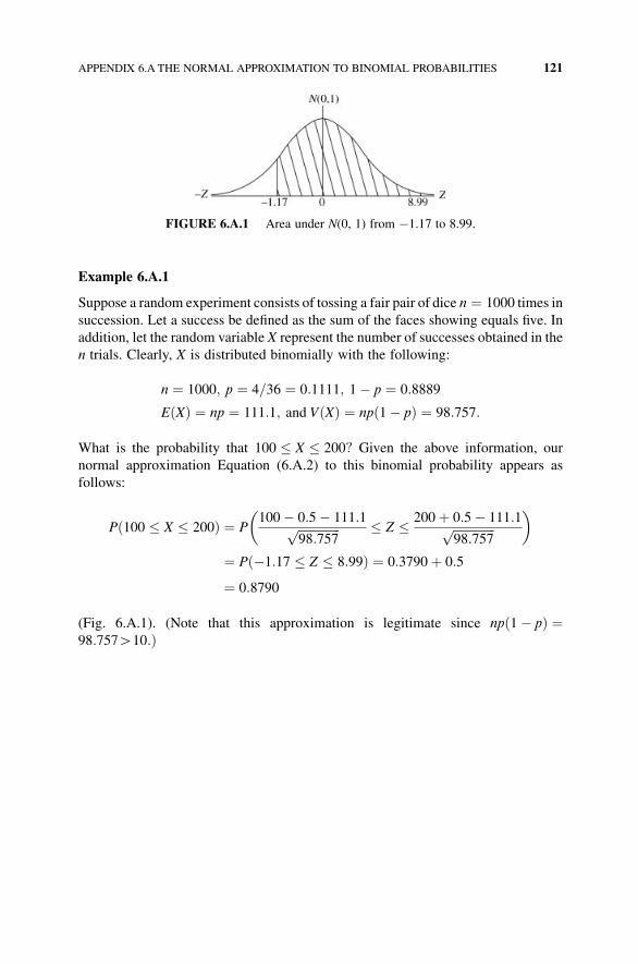
Example 6.A.1
Suppose a random experiment consists of tossing a fair pair of dice n ¼ 1000 times in
succession. Let a success be defined as the sum of the faces showing equals five. In
addition, let the random variable X represent the number of successes obtained in the
n trials. Clearly, X is distributed binomially with the following:
n ¼ 1000; p ¼ 4=36 ¼ 0:1111; 1� p ¼ 0:8889
EðXÞ ¼ np ¼ 111:1; and VðXÞ ¼ npð1� pÞ ¼ 98:757:
What is the probability that 100 � X � 200? Given the above information, our
normal approximation Equation (6.A.2) to this binomial probability appears as
follows:
Pð100 � X � 200Þ ¼ P100� 0:5� 111:1ffiffiffiffiffiffiffiffiffiffiffiffiffiffi
98:757p � Z � 200þ 0:5� 111:1ffiffiffiffiffiffiffiffiffiffiffiffiffiffi
98:757p
� �
¼ Pð�1:17 � Z � 8:99Þ ¼ 0:3790þ 0:5
¼ 0:8790
(Fig. 6.A.1). (Note that this approximation is legitimate since npð1� pÞ ¼98:757H10:Þ
FIGURE 6.A.1 Area under N(0, 1) from �1.17 to 8.99.
APPENDIX 6.A THE NORMAL APPROXIMATION TO BINOMIAL PROBABILITIES 121
7SIMPLE RANDOM SAMPLINGAND THE SAMPLING DISTRIBUTIONOF THE MEAN
7.1 SIMPLE RANDOM SAMPLING
The fundamental issue addressed by the notion of sampling is to determine when and
under what conditions a sample permits a reasonable generalization about a popu-
lation. While there are many different ways of extracting a sample from a population,
we shall primarily engage in simple random sampling. This is because, under random
sampling, we can apply the rules of probability theory to calculate the errors
associated with using a sample statistic as an estimator for a population parameter.
In what follows, we shall always sample “without replacement,” that is, once an
element of the population has been selected for inclusion in a given sample, it is no
longer eligible to appear again in that sample as the sampling process commences.
How many samples of a given size may be drawn from a given population?
Suppose the population is of size N and we are interested in taking samples of size n.
Then, since the order of the items within a sample is irrelevant (i.e., an item in the
population is either chosen or it is not—we do not care if it was picked first or last),
we can theoretically find NCn ¼ N!/n!(N� n)! possible samples. Hence there are
NCn possible ways to obtain a random sample of size n from a population of size N.
How is a random sample defined? A sample is random if each element of the
population has the same chance of being included in the sample, that is, each element
Statistical Inference: A Short Course, First Edition. Michael J. Panik.� 2012 John Wiley & Sons, Inc. Published 2012 by John Wiley & Sons, Inc.
122
of the population has a known and equal probability of being included in the sample.
Hence the probability of picking any one element of the population on the first draw is
1/N; the probability of picking any element remaining in the population on the second
draw is 1/(N� 1), and so on.
What is the probability that any one element of the population will be included in
the sample? To answer this, we need only find n/N.
What is the probability that any particular sample will be selected? This is just
1=NCn.
Now, what dowemean by simple random sampling? This is a process of sampling
that gives each possible sample combination an equal chance of being selected.
Example 7.1
Six marbles (numbered 1 through 6) are in a container. How many samples of size
three can be selected? Here N¼ 6 and n¼ 3. Thus
6C3 ¼6!
3!3!¼ 20 possible samples:
The probability of picking any one marble on draw one is 1/6; the probability of
selecting any of the remaining marbles on draw two is 1/5; and the probability of
picking any of the remainingmarbles on draw three is 1=4. The probability that any one
marble will be included in the sample is n=N ¼ 3=6 ¼ 12. And the probability that any
particular sample will be chosen is 1=6C3 ¼ 120.
As a practical matter, how do we actually extract a random sample from a (finite)
population? Those readers interested in the details of this process can consult
Appendix 7.A (using a table of random numbers). In addition, if we are provided
with a data set, how dowe know that it has been drawn randomly? A test to assess the
randomness of a particular sample appears in Appendix 10.A.
7.2 THE SAMPLING DISTRIBUTION OF THE MEAN
Suppose m is some unknown population mean. Wewant to determine its “true value.”
How should we proceed to find m? A reasonable approach is to take a simple random
sample and make an inference from the sample to the population. How is this
inference made?We use an estimator for m. Think of an estimator as a function of the
sample values used to estimate m. A logical estimator for m is the sample mean�X ¼ P
iXi=n. (Specifying an estimator is a form of data reduction—we summarize
the information about m contained in a sample by determining some essential
characteristic of the sample values. So for purposes of inference about m, we employ
the realization of �X rather than the entire set of observed data points.) Under random
sampling, �X is a random variable and thus has a probability distribution that we shall
term the sampling distribution of the mean—a distribution showing the probabilities
THE SAMPLING DISTRIBUTION OF THE MEAN 123
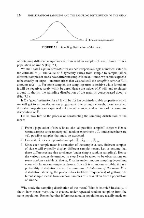
of obtaining different sample means from random samples of size n taken from a
population of size N (Fig. 7.1).
We shall call �X a point estimator for m since it reports a single numerical value as
the estimate of m. The value of �X typically varies from sample to sample (since
different samples of size n have different sample values). Hence, we cannot expect �Xto be exactly on target—an error arises that we shall call the sampling error of �X. Itamounts to �X � m. For some samples, the sampling error is positive while for others
it will be negative; rarely will it be zero. Hence the values of �X will tend to cluster
around m, that is, the sampling distribution of the mean is concentrated about m(Fig. 7.1).
Is �X a “good” estimator for m? It will be if �X has certain desirable properties (which
we will get to as our discussion progresses). Interestingly enough, these so-called
desirable properties are expressed in terms of the mean and variance of the sampling
distribution of �X.Let us now turn to the process of constructing the sampling distribution of the
mean:
1. From a population of size N let us take “all possible samples” of size n. Hence
wemust repeat some (conceptual) randomexperiment NCn times since there are
NCn possible samples that must be extracted.
2. Calculate �X for each possible sample: �X1, �X2, . . . , �XNCn.
3. Since each sample mean is a function of the sample values, different samples
of size n will typically display different sample means. Let us assume that
these differences are due to chance (under simple random sampling). Hence
the various means determined in step 2 can be taken to be observations on
some random variable �X, that is, �X varies under random sampling depending
upon which random sample is chosen. Since �X is a random variable, it has a
probability distribution called the sampling distribution of the mean �X: adistribution showing the probabilities (relative frequencies) of getting dif-
ferent sample means from random samples of size n taken from a population
of size N.
Why study the sampling distribution of the mean? What is its role? Basically, it
shows how means vary, due to chance, under repeated random sampling from the
same population. Remember that inferences about a population are usually made on
FIGURE 7.1 Sampling distribution of the mean.
124 SIMPLE RANDOM SAMPLING AND THE SAMPLING DISTRIBUTION OF THE MEAN
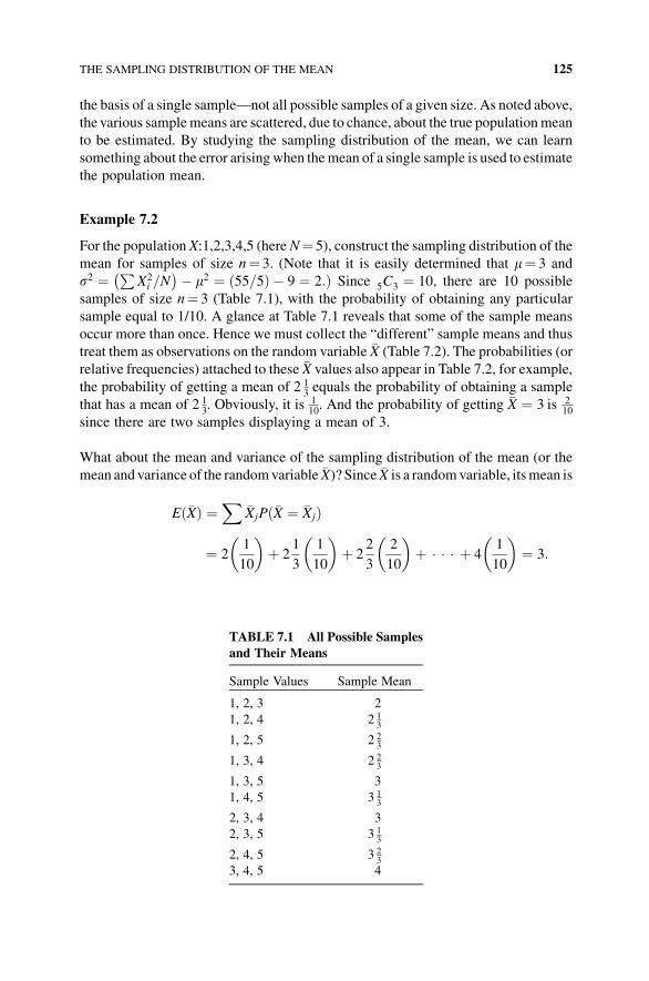
the basis of a single sample—not all possible samples of a given size. As noted above,
the various samplemeans are scattered, due to chance, about the true populationmean
to be estimated. By studying the sampling distribution of the mean, we can learn
something about the error arisingwhen themean of a single sample is used to estimate
the population mean.
Example 7.2
For the population X:1,2,3,4,5 (hereN¼ 5), construct the sampling distribution of the
mean for samples of size n¼ 3. (Note that it is easily determined that m¼ 3 and
s2 ¼ PX2i =N
� �� m2 ¼ ð55=5Þ � 9 ¼ 2:Þ Since 5C3 ¼ 10, there are 10 possible
samples of size n¼ 3 (Table 7.1), with the probability of obtaining any particular
sample equal to 1/10. A glance at Table 7.1 reveals that some of the sample means
occur more than once. Hence we must collect the “different” sample means and thus
treat them as observations on the random variable �X (Table 7.2). The probabilities (or
relative frequencies) attached to these �X values also appear in Table 7.2, for example,
the probability of getting a mean of 2 13equals the probability of obtaining a sample
that has a mean of 2 13. Obviously, it is 1
10. And the probability of getting �X ¼ 3 is 2
10
since there are two samples displaying a mean of 3.
What about the mean and variance of the sampling distribution of the mean (or the
mean and variance of the randomvariable �X)? Since �X is a randomvariable, itsmean is
Eð�XÞ ¼X
�XjPð�X ¼ �XjÞ
¼ 21
10
� �þ 2
1
3
1
10
� �þ 2
2
3
2
10
� �þ � � � þ 4
1
10
� �¼ 3:
TABLE 7.1 All Possible Samples
and Their Means
Sample Values Sample Mean
1, 2, 3 2
1, 2, 4 2 13
1, 2, 5 2 23
1, 3, 4 2 23
1, 3, 5 3
1, 4, 5 3 13
2, 3, 4 3
2, 3, 5 3 13
2, 4, 5 3 23
3, 4, 5 4
THE SAMPLING DISTRIBUTION OF THE MEAN 125
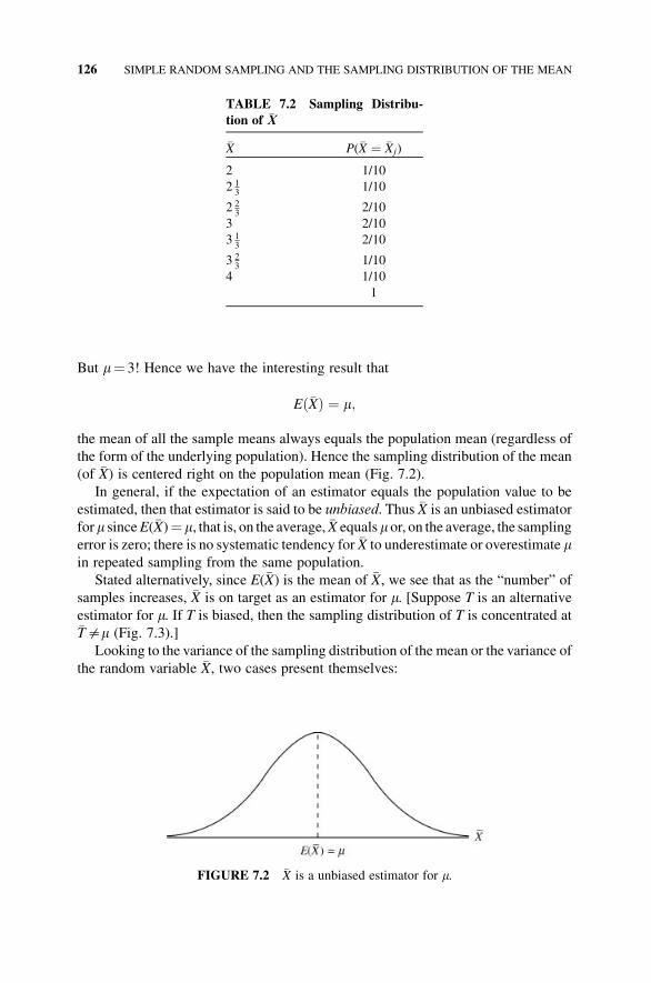
But m¼ 3! Hence we have the interesting result that
Eð�XÞ ¼ m;
the mean of all the sample means always equals the population mean (regardless of
the form of the underlying population). Hence the sampling distribution of the mean
(of �X) is centered right on the population mean (Fig. 7.2).
In general, if the expectation of an estimator equals the population value to be
estimated, then that estimator is said to be unbiased. Thus �X is an unbiased estimator
form sinceE(�X)¼ m, that is, on the average, �X equalsm or, on the average, the sampling
error is zero; there is no systematic tendency for �X to underestimate or overestimate min repeated sampling from the same population.
Stated alternatively, since E(�X) is the mean of �X, we see that as the “number” of
samples increases, �X is on target as an estimator for m. [Suppose T is an alternative
estimator for m. If T is biased, then the sampling distribution of T is concentrated at�T$m (Fig. 7.3).]
Looking to the variance of the sampling distribution of the mean or the variance of
the random variable �X, two cases present themselves:
TABLE 7.2 Sampling Distribu-
tion of �X
�X P(�X ¼ �Xj)
2 1/10
2 13
1/10
2 23
2/10
3 2/10
3 13
2/10
3 23
1/10
4 1/10
1
FIGURE 7.2 �X is a unbiased estimator for m.
126 SIMPLE RANDOM SAMPLING AND THE SAMPLING DISTRIBUTION OF THE MEAN
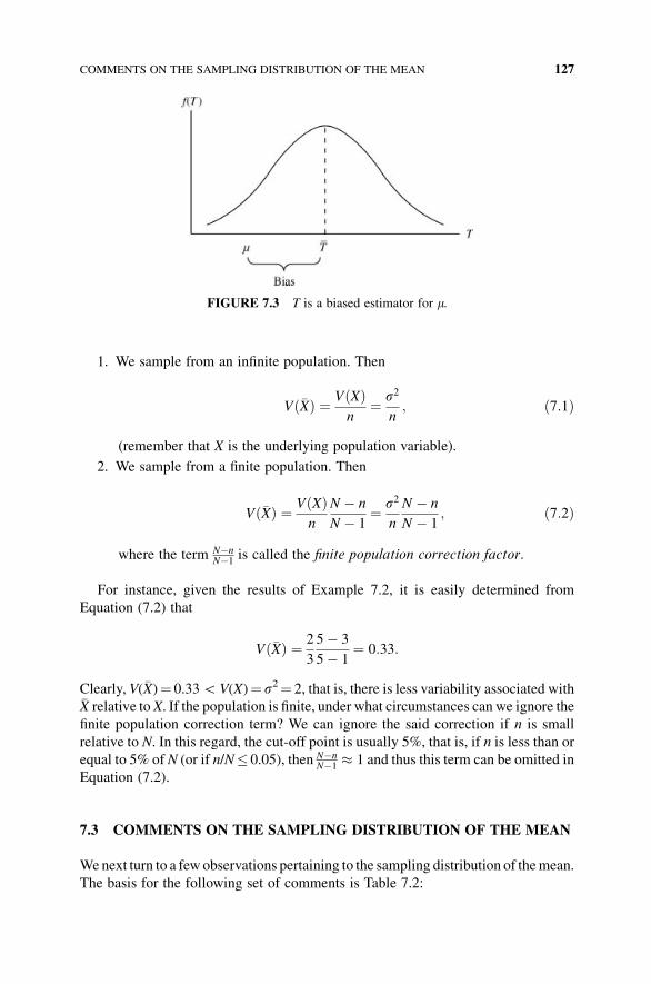
1. We sample from an infinite population. Then
Vð�XÞ ¼ VðXÞn
¼ s2
n; ð7:1Þ
(remember that X is the underlying population variable).
2. We sample from a finite population. Then
Vð�XÞ ¼ VðXÞn
N � n
N � 1¼ s2
n
N � n
N � 1; ð7:2Þ
where the term N�nN�1
is called the finite population correction factor.
For instance, given the results of Example 7.2, it is easily determined from
Equation (7.2) that
Vð�XÞ ¼ 2
3
5� 3
5� 1¼ 0:33:
Clearly, V(�X)¼ 0.33GV(X)¼ s2¼ 2, that is, there is less variability associated with�X relative to X. If the population is finite, under what circumstances can we ignore the
finite population correction term? We can ignore the said correction if n is small
relative to N. In this regard, the cut-off point is usually 5%, that is, if n is less than or
equal to 5% of N (or if n/N� 0.05), then N�nN�1
� 1 and thus this term can be omitted in
Equation (7.2).
7.3 COMMENTS ON THE SAMPLING DISTRIBUTION OF THE MEAN
Wenext turn to a few observations pertaining to the sampling distribution of themean.
The basis for the following set of comments is Table 7.2:
FIGURE 7.3 T is a biased estimator for m.
COMMENTS ON THE SAMPLING DISTRIBUTION OF THE MEAN 127
1. Each of the sample means is approximately equal to the population mean
(m¼ 3).
2. The sample means cluster much more closely about the population mean than
do the original values of X, that is, V(�X)¼ 0.33GV(X)¼ 2.
3. If larger sampleswere taken, theirmeanswould cluster evenmore closely about
the population mean than before. (To see this, let n¼ 4. Then
Vð�XÞ ¼ s2
n
N � n
N � 1¼ 2
4
5� 4
5� 1¼ 0:125:
Clearly, V(�X) has decreased in value from 0.33.) In this regard, we may
conclude that the larger the sample, the closer the sample mean is likely to
be to the population mean. This property of the sample mean is referred to as
consistency, that is, �X is a consistent estimator of m if for large samples the
probability is close to 1 that �X will be near m or
Pð�X! mÞ! 1 as n!1:
So as n increaseswithout bound, the sampling distribution of themean becomes
more and more concentrated about m.Next comes some important terminology.
4. The standard error of the mean will be calculated asffiffiffiffiffiffiffiffiffiffiffiVð�XÞ
pand will be
denoted as s�X . Clearly, the standard error of the mean is simply the standard
deviation of the distribution of sample means or of �X. Since V(�X) serves as ameasure of the average squared sampling error arising when the mean of a
single sample is used to estimate the population mean, s�X ¼ffiffiffiffiffiffiffiffiffiffiffiVð�XÞ
pis
expressed in terms of the original units of X. So given a value for s�X, wemay conclude that, on the average, the �Xjs lie approximately s�X units away
from m.(It is important to note that the term “standard error” always refers to the
“standard deviation of the sampling distribution of some statistic.”)
What factors affect the magnitude of s�X? From Equations (7.1) and (7.2),
let us first find:
(Infinite population case)
s�X ¼ sffiffiffin
p ; ð7:3Þ
(Finite population case)
s�X ¼ sffiffiffin
pffiffiffiffiffiffiffiffiffiffiffiffiN � n
N � 1
r: ð7:4Þ
128 SIMPLE RANDOM SAMPLING AND THE SAMPLING DISTRIBUTION OF THE MEAN
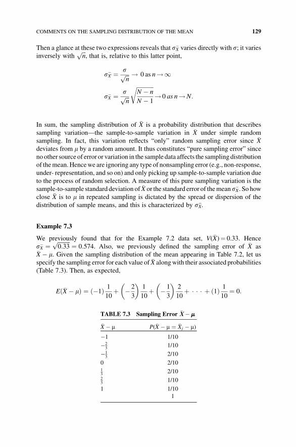
Then a glance at these two expressions reveals that s�X varies directly with s; it variesinversely with
ffiffiffin
p, that is, relative to this latter point,
s�X�¼ sffiffiffin
p ! 0 as n!1
s�X ¼ sffiffiffin
pffiffiffiffiffiffiffiffiffiffiffiffiN � n
N � 1
r! 0 as n!N:
In sum, the sampling distribution of �X is a probability distribution that describes
sampling variation—the sample-to-sample variation in �X under simple random
sampling. In fact, this variation reflects “only” random sampling error since �Xdeviates from m by a random amount. It thus constitutes “pure sampling error” since
no other source of error or variation in the sample data affects the samplingdistribution
of themean.Hencewe are ignoring any type of nonsampling error (e.g., non-response,
under- representation, and so on) and only picking up sample-to-sample variation due
to the process of random selection. A measure of this pure sampling variation is the
sample-to-sample standard deviation of �X or the standard error of themeans�X . So howclose �X is to m in repeated sampling is dictated by the spread or dispersion of the
distribution of sample means, and this is characterized by s�X.
Example 7.3
We previously found that for the Example 7.2 data set, V(�X)¼ 0.33. Hence
s�X ¼ ffiffiffiffiffiffiffiffiffi0:33
p ¼ 0:574. Also, we previously defined the sampling error of �X as�X � m. Given the sampling distribution of the mean appearing in Table 7.2, let us
specify the sampling error for each value of �X alongwith their associated probabilities
(Table 7.3). Then, as expected,
E �X � mð Þ ¼ ð�1Þ 1
10þ � 2
3
� �1
10þ � 1
3
� �2
10þ � � � þ ð1Þ 1
10¼ 0:
TABLE 7.3 Sampling Error �X� m
�X � m P(�X � m ¼ �Xj � m)
�1 1/10
�23
1/10
�13
2/10
0 2/1013
2/1023
1/10
1 1/10
1
COMMENTS ON THE SAMPLING DISTRIBUTION OF THE MEAN 129
that is, on the average, the sampling error is zero. (This is consistent with our previous
notion that Eð�XÞ ¼ m or that �X is an unbiased estimator of m.) Also,
Vð�X � mÞ ¼ E ð�X � mÞ2h i
� Eð�X � mÞ½ �2
¼ E ð�X � mÞ2h i
� 0
¼ 11
10
� �þ 4
9
1
10
� �þ 1
9
2
10
� �þ � � � þ 1
1
10
� �¼ 0:33:
Hence Vð�XÞ ¼ Vð�X � mÞ is a measure of the average squared sampling error arising
when �X estimates m; and s�X ¼ffiffiffiffiffiffiffiffiffiffiffiVð�XÞ
p¼ 0:574, that is, on the average, the individual
�Xjs are approximately 0.574 units away from m.
7.4 A CENTRAL LIMIT THEOREM
Up to this point in our discussion of the sampling distribution of themean, we have not
made any assumption about the form (shape) of the parent population. For conve-
nience, let us assume that we are sampling from an infinite population. In this regard:
1. Suppose that our population variable X is N(m, s). Then �X will be N m; s=ffiffiffin
pð Þand thus the standardized sample mean
�Z ¼�X � ms=
ffiffiffin
p isNð0; 1Þ: ð7:5Þ
Hence we can use the standard normal area table to calculate probabilities
involving �X: For instance, given that X is N(20,15) and n¼ 100, find
Pð18 � �X � 25Þ: To this end, we have
P18� 20
15=ffiffiffiffiffiffiffiffi100
p ��X � ms=
ffiffiffin
p � 25� 20
15=ffiffiffiffiffiffiffiffi100
p� �
¼ Pð�1:33 � �Z � 3:33Þ ¼ 0:4082þ 0:5 ¼ 0:9082
(See Fig. 7.4).
2. Suppose X is “not” N(m, s). Can we still use the N(0, 1) area table to calculateprobabilities involving �X? Interestingly enough, the answer is “yes” if n is
large enough. Large enough” means nH 30. The “yes” answer is provided
courtesy of the Central limit theorem: If random samples are selected from a
population with mean m and standard deviation s, then, as n increases withoutbound,
130 SIMPLE RANDOM SAMPLING AND THE SAMPLING DISTRIBUTION OF THE MEAN
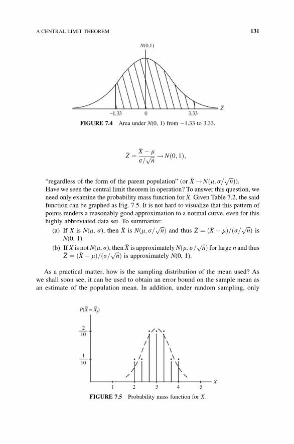
�Z ¼�X � ms=
ffiffiffin
p !Nð0; 1Þ;
“regardless of the form of the parent population” (or �X!Nðm; s= ffiffiffin
p Þ).Have we seen the central limit theorem in operation? To answer this question, we
need only examine the probability mass function for �X. Given Table 7.2, the saidfunction can be graphed as Fig. 7.5. It is not hard to visualize that this pattern of
points renders a reasonably good approximation to a normal curve, even for this
highly abbreviated data set. To summarize:
(a) If X is N(m, s), then �X is Nðm; s= ffiffiffin
p Þ and thus �Z ¼ ð�X � mÞ=ðs= ffiffiffin
p Þ isN(0, 1).
(b) If X is notN(m, s), then �X is approximatelyNðm;s= ffiffiffin
p Þ for large n and thus�Z ¼ ð�X � mÞ=ðs= ffiffiffi
np Þ is approximately N(0, 1).
As a practical matter, how is the sampling distribution of the mean used? As
we shall soon see, it can be used to obtain an error bound on the sample mean as
an estimate of the population mean. In addition, under random sampling, only
FIGURE 7.4 Area under N(0, 1) from �1.33 to 3.33.
FIGURE 7.5 Probability mass function for �X.
A CENTRAL LIMIT THEOREM 131
rarely will �X equal m exactly. Hence the sampling distribution of the mean can be
used to provide probability information about the sampling error �X � m incurred
when �X is used to estimate m. In the next chapter, these two issues are addressed
in turn.
EXERCISES
1 Suppose a population of size N¼ 5 consists of the X values: 2, 4, 6, 8, 10. If we
take all possible samples of size n¼ 2 without replacement, how many samples
will we obtain? Find the sampling distribution of the mean. Graph its probability
mass function. Next, find the following:
a. m and sb. E �Xð Þ and V �Xð Þc. The standard error of the mean
d. Verify that E �X � mð Þ ¼ 0
2 Let the population variable X beN(50, 10). What is the probability that the mean
of a sample of size n¼ 25 will differ from m by less than four units? Resolve this
problem for n¼ 50 and for n¼ 100. What can we conclude?
3 Let the populationvariableX beN(100, 10).What is the probability that themean
of a sample of size n¼ 25 will bewithin� 5 units of m? Resolve this problem for
s¼ 16. What can we conclude?
4 Suppose a population variableX consists of the values 1, 2, 3, 4, 5, 6. For samples
of size n¼ 3 taken without replacement, determine the sampling distribution of
the mean. Find E �Xð Þ and V �Xð Þ. What is the standard error of the mean?
5 Given a sample of size n¼ 64 taken from a continuous population distribution
withmean60 and standard deviation 26, find themean and variance of the sample
mean.
6 Suppose a random sample of size n¼ 10 is taken from a population that is
N(25, 8). Describe the sampling distribution of �X.
7 Suppose a random sample of size n¼ 40 is obtained from a population with a
mean of 60 and a standard deviation of 8. Must the population variable X be
normally distributed in order for the sampling distribution of the mean �Xð Þ tobe approximately normal? Why? Describe the sampling distribution of the
mean.
8 Suppose a random sample of size 15 is taken from a population with m¼ 64 and
s¼ 16.Whatmustbe true about thepopulationdistribution inorder for the normal
probability model to be applicable in determining probabilities regarding �X?
132 SIMPLE RANDOM SAMPLING AND THE SAMPLING DISTRIBUTION OF THE MEAN
Assuming this requirement to hold, describe the sampling distribution of the
mean. Also, find the following:
a. Pð�XH66Þb. P �X � 50ð Þc. P 60 � �X � 70ð Þd. P �X ¼ 57ð Þ
9 The EPA has found that the miles per gallon (mpg) for a new hybrid vehicle is N
(32, 4). Describe the sampling distribution of the mean. Additionally, find the
following:
a. The probability that a randomly selected vehicle will get at least 34mpg.
b. The probability that 10 randomly selected vehicles will have an average mpg
in excess of 33.
c. The probability that 15 randomly selected vehicles will have an average mpg
less than 30.
10 Suppose the population variable X is N(3, 0.2) and n¼ 25. How large an interval
must be chosen so that the probability is 0.95 that the sample mean �X lies
within �a units of the population mean m?
11 Suppose the population variable X is N(46, 13). How large a sample must be
taken so that the probability is 0.95 that �X will lie within �5 units of m?
12 The following n¼ 6 data values: 33.35, 34.16, 33.90, 34.55, 33.29, and 34.41
represent the times (in minutes) for a craftsman to put the finishing touches on a
table lamp. Is there any evidence to support the contention that the variable
“finishing time” is normally distributed?
APPENDIX 7.A USING A TABLE OF RANDOM NUMBERS
Suppose our objective is to obtain a simple random sample of size n from a population
of size N. One way to accomplish this task is to write the name of, say, each person in
the population on a slip of paper (or if the elements of the population are not people,
we can label each element using some identifier) and then “randomly” draw n slips of
paper out of a container.While this process might be legitimate for small populations,
it would certainly be unworkable for large ones. An alternative to this procedure is to
employ a table of random numbers (Table 7.A.1).
Let the population consist ofN¼ 10 items and supposewewant to select a random
sample of size n¼ 4. In this instance, we need to use the single digit code 0, 1, 2, . . . , 9.Given these 10 digits, we now go to the population and arbitrarily tag each of its
members with one of them. (Note that this procedure presupposes that we have at our
APPENDIX 7.A USING ATABLE OF RANDOM NUMBERS 133
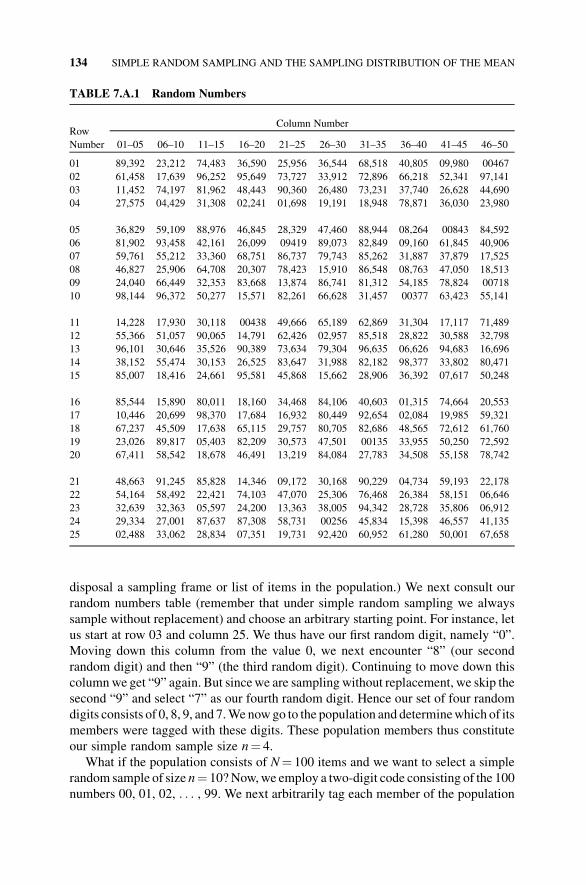
disposal a sampling frame or list of items in the population.) We next consult our
random numbers table (remember that under simple random sampling we always
sample without replacement) and choose an arbitrary starting point. For instance, let
us start at row 03 and column 25. We thus have our first random digit, namely “0”.
Moving down this column from the value 0, we next encounter “8” (our second
random digit) and then “9” (the third random digit). Continuing to move down this
columnwe get “9” again. But sincewe are sampling without replacement, we skip the
second “9” and select “7” as our fourth random digit. Hence our set of four random
digits consists of 0, 8, 9, and 7.We nowgo to the population and determinewhich of its
members were tagged with these digits. These population members thus constitute
our simple random sample size n¼ 4.
What if the population consists of N¼ 100 items and we want to select a simple
random sample of size n¼ 10?Now,we employ a two-digit code consisting of the 100
numbers 00, 01, 02, . . . , 99. We next arbitrarily tag each member of the population
TABLE 7.A.1 Random Numbers
Row
Number
Column Number
01–05 06–10 11–15 16–20 21–25 26–30 31–35 36–40 41–45 46–50
01 89,392 23,212 74,483 36,590 25,956 36,544 68,518 40,805 09,980 00467
02 61,458 17,639 96,252 95,649 73,727 33,912 72,896 66,218 52,341 97,141
03 11,452 74,197 81,962 48,443 90,360 26,480 73,231 37,740 26,628 44,690
04 27,575 04,429 31,308 02,241 01,698 19,191 18,948 78,871 36,030 23,980
05 36,829 59,109 88,976 46,845 28,329 47,460 88,944 08,264 00843 84,592
06 81,902 93,458 42,161 26,099 09419 89,073 82,849 09,160 61,845 40,906
07 59,761 55,212 33,360 68,751 86,737 79,743 85,262 31,887 37,879 17,525
08 46,827 25,906 64,708 20,307 78,423 15,910 86,548 08,763 47,050 18,513
09 24,040 66,449 32,353 83,668 13,874 86,741 81,312 54,185 78,824 00718
10 98,144 96,372 50,277 15,571 82,261 66,628 31,457 00377 63,423 55,141
11 14,228 17,930 30,118 00438 49,666 65,189 62,869 31,304 17,117 71,489
12 55,366 51,057 90,065 14,791 62,426 02,957 85,518 28,822 30,588 32,798
13 96,101 30,646 35,526 90,389 73,634 79,304 96,635 06,626 94,683 16,696
14 38,152 55,474 30,153 26,525 83,647 31,988 82,182 98,377 33,802 80,471
15 85,007 18,416 24,661 95,581 45,868 15,662 28,906 36,392 07,617 50,248
16 85,544 15,890 80,011 18,160 34,468 84,106 40,603 01,315 74,664 20,553
17 10,446 20,699 98,370 17,684 16,932 80,449 92,654 02,084 19,985 59,321
18 67,237 45,509 17,638 65,115 29,757 80,705 82,686 48,565 72,612 61,760
19 23,026 89,817 05,403 82,209 30,573 47,501 00135 33,955 50,250 72,592
20 67,411 58,542 18,678 46,491 13,219 84,084 27,783 34,508 55,158 78,742
21 48,663 91,245 85,828 14,346 09,172 30,168 90,229 04,734 59,193 22,178
22 54,164 58,492 22,421 74,103 47,070 25,306 76,468 26,384 58,151 06,646
23 32,639 32,363 05,597 24,200 13,363 38,005 94,342 28,728 35,806 06,912
24 29,334 27,001 87,637 87,308 58,731 00256 45,834 15,398 46,557 41,135
25 02,488 33,062 28,834 07,351 19,731 92,420 60,952 61,280 50,001 67,658
134 SIMPLE RANDOM SAMPLING AND THE SAMPLING DISTRIBUTION OF THE MEAN
with one of these two-digit numbers. Again, our starting point in Table 7.A.1 is
arbitrary. Suppose we start with row 05 and columns 21 and 22. Our first random
number is thus “28.” Moving down these columns from 28 we see that our complete
sequence of n¼ 10 random numbers is
28; 09; 86; 78; 13; 82; 49; 62; 73; 83:
We now go back to the population and select those members that have been tagged
with these 10 two-digit random numbers. They constitute our simple random sample
of size n¼ 10.
If our population had N¼ 1000 items and we wanted to obtain a simple random
sample of size n¼ 25, then our requisite three-digit code would involve the 1000
numbers 000, 001, 002, . . . , 999. Next, the population members are arbitrarily tagged
with these three-digit numbers and a trip to Table 7.A.1 has us choose an arbitrary
starting point (e.g., our first randomnumber could be chosen from row01 and columns
3, 4, and 5 or “392”). Moving down these columns away from 392 enables us to select
24 additional three-digit random numbers so that our entire set of 25 three-digit
random numbers consists of the following:
392 902 228 544 663
458 761 366 446 164
452 827 101 237 639
575 010 152 026 334
829 144 007 411 488
We now revisit the population and determine which of its members received these
three-digit numbers. These members thus make up our random sample of n¼ 25
items.
Given that a bona fide table of random numbers is unavailable, what is the
next best thing to use? How about a telephone directory? (Not the Yellow
Pages.) The last four digits of any telephone number are not assigned on a
systematic basis. Hence one need only arbitrarily pick a page and a column
within it, find a starting point, and then move down the column(s) to extract a set
of random numbers.
Suppose that one does not have a well-defined sampling frame or list of items
within the population. Then a sampling process called systematic random sampling
will work nicely. Specifically, to obtain a systematic random sample, select every kth
member from the population (k is termed the sampling cycle), with the first member
selected by choosing a randomnumber between 1 andk.More formally, the process of
extracting a systematic random sample of size n from a population of known sizeN is
as follows:
1. Round the quantity N/n down to the nearest integer. This gives the sampling
cycle k.
APPENDIX 7.A USING ATABLE OF RANDOM NUMBERS 135
2. Randomly select a number p between 1 and k.
3. Hence the pth item in the population is selected along with every kth member
thereafter. Our systematic random sample thus consists of the following
population elements:
p; pþ k; pþ 2 k; . . . ; pþ ðn� 1Þ k:
4. This sampling process commences until we have selected n items from the
population.
If N is not known, then k cannot be calculated—kmust be determined judiciously so
that a representative sample is obtained, that is, k should not be so large that n is
unattainable; or k should not be so small that only a narrow slice of the population or a
biased sample results. It is important to note that for systematic random sampling to be
effective, the items in the population should be arranged in a random fashion to begin
with. For instance, weekend shoppers exiting a suburban mall could be considered a
random population as also the alphabetical listing of students enrolled at a local
community college.
Example 7.A.1
Suppose that we want to obtain a simple random sample of size n¼ 35 from a
population whose size is estimated to be N¼ 600. Under systematic random sam-
pling,N/n¼ 600/35¼ 17.4� 17¼ k. Let us randomly select a number between 1 and
17. Let us say it is “10.” Then we select the 10th member of the population and every
17th member thereafter, until a sample of 35 items is achieved. Thus our sample of
size n¼ 35 consists of the elements positioned or ordered as follows:
10; 27; 44; 61; 78; . . . ; 588
where 588¼ p þ (n� 1) k¼ 10 þ 34 (17).
Given that we now know how to acquire a simple random sample, we may go a step
further and check to see if any such sample data set can be treated “as if” it was drawn
from a normal population. This is the task of Appendix 7.B.
APPENDIX 7.B ASSESSING NORMALITY VIA THE NORMAL
PROBABILITY PLOT
How can we determine if a simple random sample taken from some unknown
population is normally distributed (or approximately so)? One way to answer this
question is to see if the sample data values plot out as a frequency distribution that is
bell-shaped and symmetrical. As one might expect, for large data sets, a distinct
normal pattern may emerge that would lead one to conclude that the underlying
136 SIMPLE RANDOM SAMPLING AND THE SAMPLING DISTRIBUTION OF THE MEAN
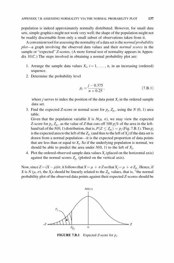
population is indeed approximately normally distributed. However, for small data
sets, simple graphics might not work very well; the shape of the population might not
be readily discernable from only a small subset of observations taken from it.
A convenient tool for assessing the normality of a data set is the normal probability
plot—a graph involving the observed data values and their normal scores in the
sample or “expected” Z-scores. (A more formal test of normality appears in Appen-
dix 10.C.) The steps involved in obtaining a normal probability plot are:
1. Arrange the sample data values Xi, i¼ 1, . . . , n, in an increasing (ordered)
sequence.
2. Determine the probability level
pj ¼ j � 0:375
nþ 0:25; ð7:B:1Þ
where j serves to index the position of the data point Xi in the ordered sample
data set.
3. Find the expected Z-score or normal score for pj, Zpj ; using the N (0, 1) area
table.
Given that the population variable X is N(m, s), we may view the expected
Z-score for pj, Zpj ; as the value of Z that cuts off 100 pj% of the area in the left-
hand tail of theN(0, 1) distribution, that is,PðZ � Zpj Þ ¼ pj (Fig. 7.B.1). Thus pjis the expected area to the left of theZpj (and thus to the left ofXj) if the data set is
drawn from a normal population—it is the expected proportion of data points
that are less than or equal to Xj. So if the underlying population is normal, we
should be able to predict the area under N(0, 1) to the left of Xj.
4. Plot the ordered observed sample data values Xj (placed on the horizontal axis)
against the normal scores Zpj (plotted on the vertical axis).
Now, since Z¼ (X� m)/s, it follows thatX¼ m þ s Z so thatXj¼ m þ sZpj . Hence, ifX is N (m, s), the Xjs should be linearly related to the Zpj values, that is, “the normal
probability plot of the observed data points against their expected Z-scores should be
FIGURE 7.B.1 Expected Z-score for pj.
APPENDIX 7.B ASSESSING NORMALITY VIA THE NORMAL PROBABILITY PLOT 137
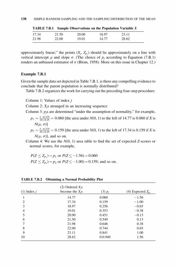
approximately linear;” the points (Xj, Zpj ) should lie approximately on a line with
vertical intercept m and slope s. (The choice of pj according to Equation (7.B.1)
renders an unbiased estimator of s (Blom, 1958). More on this issue in Chapter 12.)
Example 7.B.1
Given the sample data set depicted in Table 7.B.1, is there any compelling evidence to
conclude that the parent population is normally distributed?
Table 7.B.2 organizes thework for carrying out the preceding four-step procedure:
Column 1: Values of index j
Column 2: Xjs arranged in an increasing sequence
Column 3: pjs are determined “under the assumption of normality,” for example,
p1 ¼ 1�0:37510þ0:25 ¼ 0:060 [the area under N(0, 1) to the left of 14.77 is 0.060 if X is
N(m, s)]
p2 ¼ 2�0:37510þ0:25 ¼ 0:159 [the area under N(0, 1) to the left of 17.34 is 0.159 if X is
N(m, s)], and so on.
Column 4: We use the N(0, 1) area table to find the set of expected Z-scores or
normal scores, for example,
P(Z � Zp1 )¼ p1 or P(Z��1.56)¼ 0.060
P(Z � Zp2 )¼ p2 or P(Z��1.00)¼ 0.159; and so on.
TABLE 7.B.1 Sample Observations on the Population Variable X
17.34 21.50 20.00 18.97 23.11
21.98 22.00 19.01 14.77 28.62
TABLE 7.B.2 Obtaining a Normal Probability Plot
(1) Index j
(2) Ordered Xis
become the Xjs (3) pj (4) Expected Zpj
1 14.77 0.060 �1.56
2 17.34 0.159 �1.00
3 18.97 0.256 �0.65
4 19.01 0.353 �0.38
5 20.00 0.451 �0.13
6 21.50 0.549 0.13
7 21.98 0.646 0.38
8 22.00 0.744 0.65
9 23.11 0.841 1.00
10 28.62 0.0.940 1.56
138 SIMPLE RANDOM SAMPLING AND THE SAMPLING DISTRIBUTION OF THE MEAN
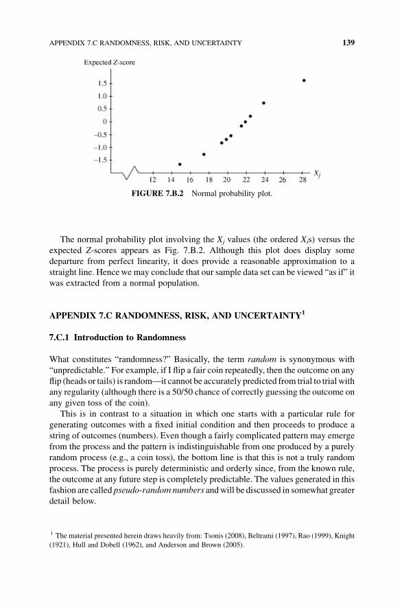
The normal probability plot involving the Xj values (the ordered Xis) versus the
expected Z-scores appears as Fig. 7.B.2. Although this plot does display some
departure from perfect linearity, it does provide a reasonable approximation to a
straight line. Hencewe may conclude that our sample data set can be viewed “as if” it
was extracted from a normal population.
APPENDIX 7.C RANDOMNESS, RISK, AND UNCERTAINTY1
7.C.1 Introduction to Randomness
What constitutes “randomness?” Basically, the term random is synonymous with
“unpredictable.” For example, if I flip a fair coin repeatedly, then the outcome on any
flip (heads or tails) is random—it cannot be accurately predicted from trial to trial with
any regularity (although there is a 50/50 chance of correctly guessing the outcome on
any given toss of the coin).
This is in contrast to a situation in which one starts with a particular rule for
generating outcomes with a fixed initial condition and then proceeds to produce a
string of outcomes (numbers). Even though a fairly complicated pattern may emerge
from the process and the pattern is indistinguishable from one produced by a purely
random process (e.g., a coin toss), the bottom line is that this is not a truly random
process. The process is purely deterministic and orderly since, from the known rule,
the outcome at any future step is completely predictable. The values generated in this
fashion are called pseudo-randomnumbers andwill be discussed in somewhat greater
detail below.
FIGURE 7.B.2 Normal probability plot.
1 The material presented herein draws heavily from: Tsonis (2008), Beltrami (1997), Rao (1999), Knight
(1921), Hull and Dobell (1962), and Anderson and Brown (2005).
APPENDIX 7.C RANDOMNESS, RISK, AND UNCERTAINTY 139

What ifwe observe a string of outcomes (ostensibly random) butwe donot have the
rule that produced it? If we can encode the pattern of outcomes and ultimately find
the rule, then here too we can predict the system’s behavior over time and thus pure
randomness is not present. Note that in order to predict a future outcome, all steps
leading to that outcome have to be explicitly calculated. But if no specific rule(s) can
be discovered, then, in this instance, the string of outcomes is truly unpredictable and
thus can be considered as random, that is, we can treat the string of values “as if” it
were generated by a purely random process.
As indicated above, randomness reflects the unpredictability of an event; an
outcome or event occurs without discernible design or cause. Randomness is a part
of everyday life; we are typically concerned about the weather, worried about the
morning bus being late because of traffic problems, anxious about how one’s 401k
planwill fare thismonth, and so on. Randomness can be a source of amusement (will I
win tonight’s lottery drawing or this week’s office sports pool?) as well as trepidation
(will the “big quake” hit the San Francisco area during my upcoming visit there?).
And it can possibly serve as a safeguard against boredom (onemaymuse: “Maybe I’ll
meet some interesting people today in my job as receptionist?”).
At first blush, randomness may be thought to possess the qualities of confusion,
disorder, something jumbled or scrambled, and disorganization. This view of
randomness is, however, much too na€ıve. Randomness is actually steeped in “rules.”
While the rule may be obvious (flipping a coin to get heads or tails) or hidden from us
(the physical world is typically known imperfectly), the resulting outcomes are
uncertain and thus unpredictable—we cannot perceive a cause or detect any pattern of
behavior or semblance of order. This is what is meant when someone says: “The
incident happened by blind chance.” Here some outcome occurs at the intersection of
an unlimited number of supposedly unrelated events, with each of these events
occurring because of happenstance. Such contingent circumstances are thought to
reflect unintentional accidents or are viewed as “an act of God” (some predetermined
plan is being carried out via “divine intervention”).
Many attempts have been made to thwart the vicissitudes of uncertainty. The
ancients attempted to divine and evenundermine the “will of theGods” by engaging in
games of chance. They believed that gaming or the simulation of the Gods’ uncertain
behavior would reveal the outcomes that “higher powers” had in store for them. Thus
“fate” and “destiny,” as directed by “divine intent,” might be modified or even
obstructed.
A more sophisticated attempt to harness uncertainty was made with the advent of
probability theory. Now, one could achieve a fuller understanding of the patterns
of outcomes due to chance by expressing in mathematical form the likelihood of
occurrence of events. Probability theory served as the vehicle for separating in a
precise fashion probable from improbable outcomes. Thus the disorder of belief in
fateful happenings was replaced by a methodical way of assessing the odds of chance
outcomes.
Armed with these new analytical tools, randomness was eventually regarded
in a more pragmatic light. Certainly, misfortune and disruptions are still with us
(e.g., natural disasters, economic dislocations, acts of terror and mindless violence,
140 SIMPLE RANDOM SAMPLING AND THE SAMPLING DISTRIBUTION OF THE MEAN
physical and mental health problems, and so on). However, randomness soon came
to be viewed as a crucial or even healthy medium for the development and/or
sustainability of life-enhancing processes. In this regard, uncertainty can be thought
of as necessary for the spawning of innovation and diversity; it is a mechanism that
sets in motion evolutionary adaptations and sparks the processes that are essential
for the renewal of life. A confluence of chance factors may ensure the viability of
different life forms and the resiliency of entire ecosystems. That is, chance
disruptions (mutations or accidents of nature) in the physical world provide the
raw material for natural selection in the long run. Environmental conditions favor or
inhibit the development or survival of specific individuals or species. Thus it is
happenstance that can alter the path of evolution; some species adapt and thrive
while others disappear.
We know that if an individual number is random, then its value is unpredictable.
Additionally, any such number must be drawn from a set of equiprobable values (e.g.,
it is obtained from, say, a uniform probability distribution). But when considering a
sequence of random numbers, each element drawn from the sequence must be
statistically independent of the others.
While randomness is inherent in the physical world (think of collisions between
subatomic particles), it is also the case that uncertainty has served as the basis for
developing theories of societal behavior. Although uncertainties exist at the
individual level, a modicum of stability is present in the average behavior of a
collection of individuals. This conclusion, reflecting order in disorder, emerges
due to the Law of Large Numbers. That is, the degree of uncertainty in the average
performance of individuals in a system decreases as the number of individuals
increase so that the system as a whole exhibits a virtually deterministic form of
behavior.
For instance, suppose a large number of individuals are asked to estimate, by sight,
the length of an object. Certainly, somewill overestimate the length while others will
underestimate it. And some of these individuals will be close to the true length while
others will be a bit farther from it. Each estimate can be treated as a random number—
we cannot predict with any degree of certainty the value that any given person will
state. Moreover, each individual is assumed to guess the length of the object
independently of the others. So given that positive and negative deviations from the
true length are equally likely and no one value can be expected to predominate, we
expect that the actual measurements are normally distributed about the true length of
the object or the measurement errors are normally distributed about zero. Thus small
errors are likely to occur more frequently than large ones and very large errors are
highly unlikely.
So while we cannot predict the actual type of measurement error that a single
individual will make, we can predict, with a reasonable degree of certainty, how the
errors resulting from measurements made by a large number of individuals behave:
more people will make small errors than large ones; the larger the error, the fewer the
number of people making it; approximately, the same number of individuals will
overestimate as will underestimate the actual length; and the average error, taken over
all individuals, will be zero.
APPENDIX 7.C RANDOMNESS, RISK, AND UNCERTAINTY 141
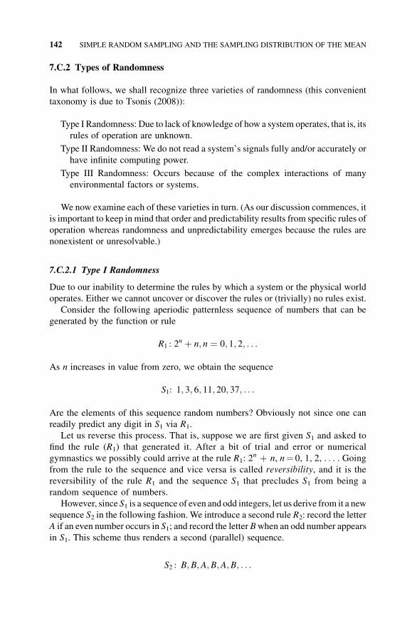
7.C.2 Types of Randomness
In what follows, we shall recognize three varieties of randomness (this convenient
taxonomy is due to Tsonis (2008)):
Type I Randomness: Due to lack of knowledge of how a system operates, that is, its
rules of operation are unknown.
Type II Randomness: We do not read a system’s signals fully and/or accurately or
have infinite computing power.
Type III Randomness: Occurs because of the complex interactions of many
environmental factors or systems.
We now examine each of these varieties in turn. (As our discussion commences, it
is important to keep in mind that order and predictability results from specific rules of
operation whereas randomness and unpredictability emerges because the rules are
nonexistent or unresolvable.)
7.C.2.1 Type I Randomness
Due to our inability to determine the rules by which a system or the physical world
operates. Either we cannot uncover or discover the rules or (trivially) no rules exist.
Consider the following aperiodic patternless sequence of numbers that can be
generated by the function or rule
R1 : 2n þ n; n ¼ 0; 1; 2; . . .
As n increases in value from zero, we obtain the sequence
S1: 1; 3; 6; 11; 20; 37; . . .
Are the elements of this sequence random numbers? Obviously not since one can
readily predict any digit in S1 via R1.
Let us reverse this process. That is, suppose we are first given S1 and asked to
find the rule (R1) that generated it. After a bit of trial and error or numerical
gymnastics we possibly could arrive at the rule R1: 2n þ n, n¼ 0, 1, 2, . . . . Going
from the rule to the sequence and vice versa is called reversibility, and it is the
reversibility of the rule R1 and the sequence S1 that precludes S1 from being a
random sequence of numbers.
However, since S1 is a sequence of even and odd integers, let us derive from it a new
sequence S2 in the following fashion. We introduce a second rule R2: record the letter
A if an even number occurs in S1; and record the letter Bwhen an odd number appears
in S1. This scheme thus renders a second (parallel) sequence.
S2 : B;B;A;B;A;B; . . .
142 SIMPLE RANDOM SAMPLING AND THE SAMPLING DISTRIBUTION OF THE MEAN
Now, supposewewere provided with S2 but not the ruleR2 that generated it. It is quite
possible that we could conclude that the A’s and B’s represent even and odd numbers,
respectively, so that reversibility between S2 andR2 holds. However, reversibility does
not hold betweenR2 and S1—for eachA (respectively,B), there is an infinite number of
even numbers (respectively, odd numbers) to choose from.And sinceR2 introduces an
element of uncertainty into the system that prevents us from uncovering R1, we see
that S2 can be treated as a random sequence.
The upshot of this discussion is that if we observe an aperodic patternless sequence
that has been generated by some rule that we are not able to uncover, then clearly we
donot have the ability to predict future elements of the sequence and thus the sequence
in question can be treated as random. For all intents and purposes, the sequence under
discussion is no different from a purely random sequence if reversibility between the
sequence and some rule that produced it does not hold. So if we experience
irreversible processes that preclude us from discovering the rules of a system’s
operation, and we don’t simply find ourselves in some circumstance in which rules do
not exist, then the condition of unpredictability and thus randomness prevails.
7.C.2.2 Type II Randomness
Due to lack of infinite precision and computing power. Suppose we have a nonlinear
albeit deterministic model (or rule) described by an iterative process in which the
value Xnþ 1 is determined from the previous value Xn, n¼ 0, 1, 2, . . . .For n¼ 0, Xo is our initial condition. Let Xo¼ 0.06517. Now, let us change the
initial condition slightly, for example, Xo¼ 0.06517 is replaced by Xo¼ 0.06500.
Surprisingly, the two paths of the system (one with the initial condition 0.06517 and
the other with the initial condition 0.06500) may be radically different (due to the
nonlinearity of the process) and thus may not converge (if they converge at all) to the
same value. The key notion here is that the system is highly sensitive to the initial
conditions chosen. In fact, even for miniscule perturbations or errors of measurement
of the initial conditions, the end results become highly unpredictable and thus random.
Clearly lack of precision, as reflected by using convenient or inexact approx-
imations to initial conditions, influences the evolution of a nonlinear system or
model, thus leading to an outcome that ismuch different from, say, previous ones. To
avoid this circumstance and to make “on-target” predictions, infinite precision and
infinite computing power is needed. Since we lack such resources, the exact state of
the system after a few iterations will be unknown and consequently unpredictable,
thus rendering all future states random or unpredictable as well. Thus randomness
emerges even if the rules are known and/or the system is reversible. In fact, this state
of affairs, in which sensitivity to initial conditions is important, is termed chaotic
(more on that later).
7.C.2.3 Type III Randomness
Due to the continuing impact of the environment. Suppose we have a fixed period of
time (in hours) in which to drive at the posted speed limit. How far will we travel in a
given direction? Here time� speed¼ distance traveled. It should be evident that
APPENDIX 7.C RANDOMNESS, RISK, AND UNCERTAINTY 143
“distance” is a random number since the traffic patterns, slow-downs/stops, possible
accident delays, and so on are unpredictable. So, even though “time” and “speed” are
specified and thus deterministic, “distance” is not fully knowable and thus is
considered random.
What is the mechanism by which randomness is introduced into the system? Here
randomness is injected into the operation of the system via the interaction of external
environmental factors or players whose actions are beyond our control, for example,
stop signs, other drivers, traffic lights, the right-of-way of emergency vehicles, and so
on, obviously adversely impact distance traveled. Taken collectively, these environ-
mental factors interact in a complex fashion to produce a process of operation that is
essentially a random process.
Interestingly enough, as the preceding example illustrates, Type III Randomness
can emerge even if we start with no randomness at all. A system that exhibits regular
behavior can eventually display complicated behaviorwhen it is subject to an external
force that might also be very regular. Hence the operation of very simple rules of
behavior, when exposed to other such rules, can, in combination, precipitate unpre-
dictability. The collective behavior of interacting nonrandom environmental factors
can produce randomness.
7.C.3 Pseudo-Random Numbers
Natural random numbers occur in an “innate” way, that is, they are generated by one
of nature’s physical processes such as: tracking successive male (we record a 1) and
female (we record a 0) births at a hospital; tracing the path of a neutron or some other
particle that is subject to random collisions; arrivals at a toll booth; counting the
particles emitted by the decay of a radioactive element; atmospheric noise, and so on.
In these examples, randomness is “inherent” and any calculation of these numbers
involves a simulation of the underlying physical process involved.
Artificially generated random numbers are obtained by using a chance mech-
anism such as: flipping a fair coin; rolling a fair pair of dice; drawing tokens
numbered 0, 1, . . . , 9 from a bag, one by one, under replacement; using a suitable
probability distribution, and so on. Whether a random number has been produced
naturally or artificially is inconsequential—each is thought to be a true or pure
random number.
It is more or less the current belief in the mathematics community that, in order to
obtain a valid sequence of randomnumbers, one should not rely on natural procedures
but, instead, on suitably deterministic ones. Random numbers generated in this
fashion (typically with the use of a computer) are termed pseudo-random numbers.
Sequences of such numbers, which are obtained via a software function, are called
pseudo-random because they are actually deterministic in nature, that is, given a
specific source function and a fixed seed (starting) value, the same sequence of
numbers can be generated time after time. If the pseudo-random number source
function is well-designed, then the resulting sequence of numbers will appear to be
truly random (provided that the sequence does not repeat too often). In fact, the
144 SIMPLE RANDOM SAMPLING AND THE SAMPLING DISTRIBUTION OF THE MEAN
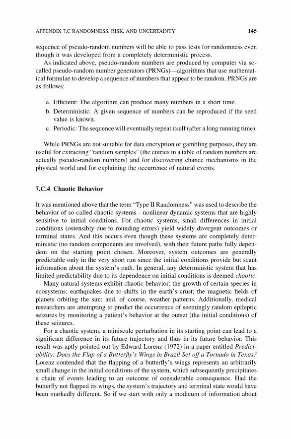
sequence of pseudo-random numbers will be able to pass tests for randomness even
though it was developed from a completely deterministic process.
As indicated above, pseudo-random numbers are produced by computer via so-
called pseudo-random number generators (PRNGs)—algorithms that use mathemat-
ical formulae to develop a sequence of numbers that appear to be random. PRNGs are
as follows:
a. Efficient: The algorithm can produce many numbers in a short time.
b. Deterministic: A given sequence of numbers can be reproduced if the seed
value is known.
c. Periodic: The sequencewill eventually repeat itself (after a long running time).
While PRNGs are not suitable for data encryption or gambling purposes, they are
useful for extracting “random samples” (the entries in a table of random numbers are
actually pseudo-random numbers) and for discovering chance mechanisms in the
physical world and for explaining the occurrence of natural events.
7.C.4 Chaotic Behavior
It was mentioned above that the term “Type II Randomness” was used to describe the
behavior of so-called chaotic systems—nonlinear dynamic systems that are highly
sensitive to initial conditions. For chaotic systems, small differences in initial
conditions (ostensibly due to rounding errors) yield widely divergent outcomes or
terminal states. And this occurs even though these systems are completely deter-
ministic (no random components are involved), with their future paths fully depen-
dent on the starting point chosen. Moreover, system outcomes are generally
predictable only in the very short run since the initial conditions provide but scant
information about the system’s path. In general, any deterministic system that has
limited predictability due to its dependence on initial conditions is deemed chaotic.
Many natural systems exhibit chaotic behavior: the growth of certain species in
ecosystems; earthquakes due to shifts in the earth’s crust; the magnetic fields of
planets orbiting the sun; and, of course, weather patterns. Additionally, medical
researchers are attempting to predict the occurrence of seemingly random epileptic
seizures by monitoring a patient’s behavior at the outset (the initial conditions) of
these seizures.
For a chaotic system, a miniscule perturbation in its starting point can lead to a
significant difference in its future trajectory and thus in its future behavior. This
result was aptly pointed out by Edward Lorenz (1972) in a paper entitled Predict-
ability: Does the Flap of a Butterfly’s Wings in Brazil Set off a Tornado in Texas?
Lorenz contended that the flapping of a butterfly’s wings represents an arbitrarily
small change in the initial conditions of the system, which subsequently precipitates
a chain of events leading to an outcome of considerable consequence. Had the
butterfly not flapped its wings, the system’s trajectory and terminal state would have
been markedly different. So if we start with only a modicum of information about
APPENDIX 7.C RANDOMNESS, RISK, AND UNCERTAINTY 145
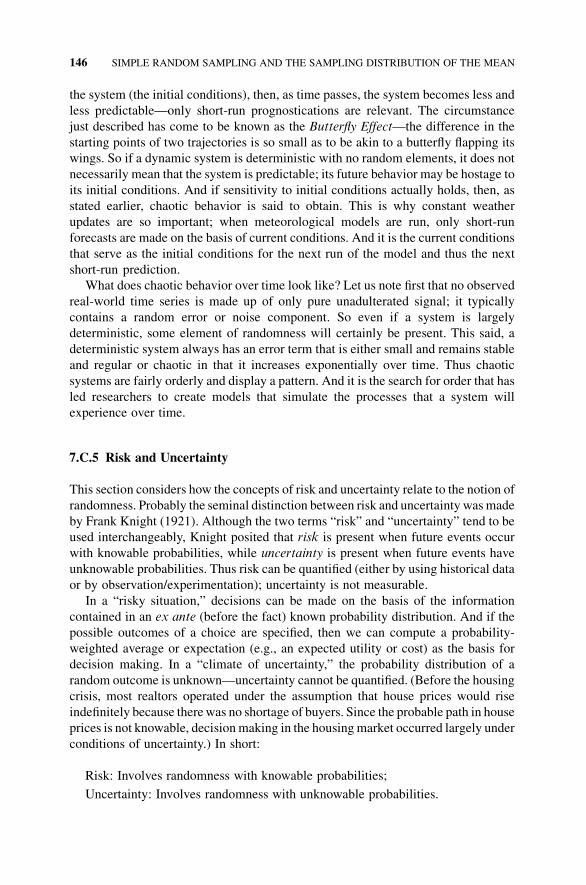
the system (the initial conditions), then, as time passes, the system becomes less and
less predictable—only short-run prognostications are relevant. The circumstance
just described has come to be known as the Butterfly Effect—the difference in the
starting points of two trajectories is so small as to be akin to a butterfly flapping its
wings. So if a dynamic system is deterministic with no random elements, it does not
necessarily mean that the system is predictable; its future behavior may be hostage to
its initial conditions. And if sensitivity to initial conditions actually holds, then, as
stated earlier, chaotic behavior is said to obtain. This is why constant weather
updates are so important; when meteorological models are run, only short-run
forecasts are made on the basis of current conditions. And it is the current conditions
that serve as the initial conditions for the next run of the model and thus the next
short-run prediction.
What does chaotic behavior over time look like? Let us note first that no observed
real-world time series is made up of only pure unadulterated signal; it typically
contains a random error or noise component. So even if a system is largely
deterministic, some element of randomness will certainly be present. This said, a
deterministic system always has an error term that is either small and remains stable
and regular or chaotic in that it increases exponentially over time. Thus chaotic
systems are fairly orderly and display a pattern. And it is the search for order that has
led researchers to create models that simulate the processes that a system will
experience over time.
7.C.5 Risk and Uncertainty
This section considers how the concepts of risk and uncertainty relate to the notion of
randomness. Probably the seminal distinction between risk and uncertainty wasmade
by Frank Knight (1921). Although the two terms “risk” and “uncertainty” tend to be
used interchangeably, Knight posited that risk is present when future events occur
with knowable probabilities, while uncertainty is present when future events have
unknowable probabilities. Thus risk can be quantified (either by using historical data
or by observation/experimentation); uncertainty is not measurable.
In a “risky situation,” decisions can be made on the basis of the information
contained in an ex ante (before the fact) known probability distribution. And if the
possible outcomes of a choice are specified, then we can compute a probability-
weighted average or expectation (e.g., an expected utility or cost) as the basis for
decision making. In a “climate of uncertainty,” the probability distribution of a
random outcome is unknown—uncertainty cannot be quantified. (Before the housing
crisis, most realtors operated under the assumption that house prices would rise
indefinitely because therewas no shortage of buyers. Since the probable path in house
prices is not knowable, decisionmaking in the housingmarket occurred largely under
conditions of uncertainty.) In short:
Risk: Involves randomness with knowable probabilities;
Uncertainty: Involves randomness with unknowable probabilities.
146 SIMPLE RANDOM SAMPLING AND THE SAMPLING DISTRIBUTION OF THE MEAN
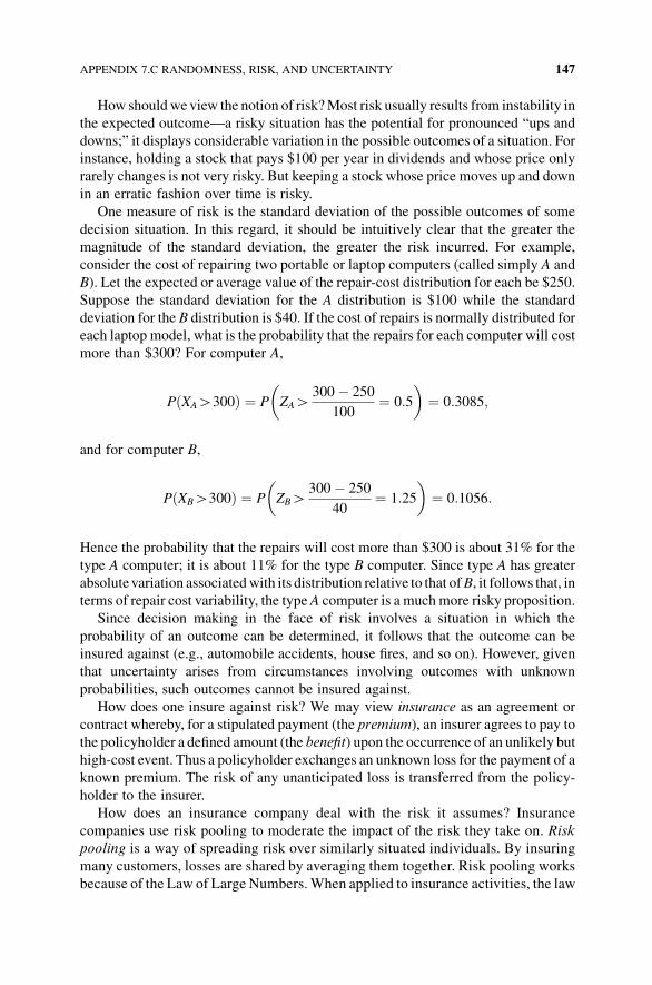
How shouldweview the notion of risk?Most risk usually results from instability in
the expected outcome—a risky situation has the potential for pronounced “ups and
downs;” it displays considerable variation in the possible outcomes of a situation. For
instance, holding a stock that pays $100 per year in dividends and whose price only
rarely changes is not very risky. But keeping a stock whose price moves up and down
in an erratic fashion over time is risky.
One measure of risk is the standard deviation of the possible outcomes of some
decision situation. In this regard, it should be intuitively clear that the greater the
magnitude of the standard deviation, the greater the risk incurred. For example,
consider the cost of repairing two portable or laptop computers (called simply A and
B). Let the expected or average value of the repair-cost distribution for each be $250.
Suppose the standard deviation for the A distribution is $100 while the standard
deviation for the B distribution is $40. If the cost of repairs is normally distributed for
each laptop model, what is the probability that the repairs for each computer will cost
more than $300? For computer A,
PðXAH300Þ ¼ P ZAH300� 250
100¼ 0:5
� �¼ 0:3085;
and for computer B,
PðXBH300Þ ¼ P ZBH300� 250
40¼ 1:25
� �¼ 0:1056:
Hence the probability that the repairs will cost more than $300 is about 31% for the
type A computer; it is about 11% for the type B computer. Since type A has greater
absolute variation associatedwith its distribution relative to that ofB, it follows that, in
terms of repair cost variability, the type A computer is a muchmore risky proposition.
Since decision making in the face of risk involves a situation in which the
probability of an outcome can be determined, it follows that the outcome can be
insured against (e.g., automobile accidents, house fires, and so on). However, given
that uncertainty arises from circumstances involving outcomes with unknown
probabilities, such outcomes cannot be insured against.
How does one insure against risk? We may view insurance as an agreement or
contract whereby, for a stipulated payment (the premium), an insurer agrees to pay to
the policyholder a defined amount (the benefit) upon the occurrence of an unlikely but
high-cost event. Thus a policyholder exchanges an unknown loss for the payment of a
known premium. The risk of any unanticipated loss is transferred from the policy-
holder to the insurer.
How does an insurance company deal with the risk it assumes? Insurance
companies use risk pooling to moderate the impact of the risk they take on. Risk
pooling is a way of spreading risk over similarly situated individuals. By insuring
many customers, losses are shared by averaging them together. Risk pooling works
because of the Law of Large Numbers.When applied to insurance activities, the law
APPENDIX 7.C RANDOMNESS, RISK, AND UNCERTAINTY 147
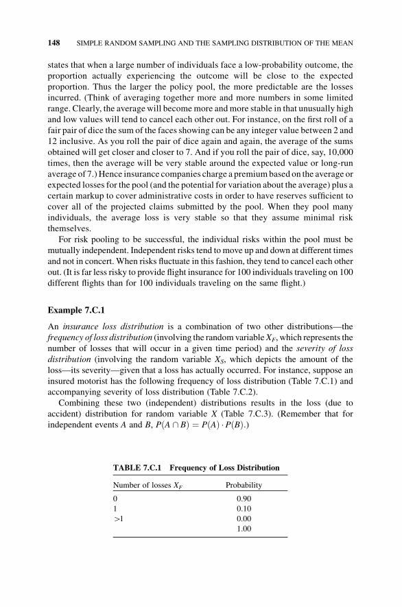
states that when a large number of individuals face a low-probability outcome, the
proportion actually experiencing the outcome will be close to the expected
proportion. Thus the larger the policy pool, the more predictable are the losses
incurred. (Think of averaging together more and more numbers in some limited
range. Clearly, the averagewill becomemore andmore stable in that unusually high
and low values will tend to cancel each other out. For instance, on the first roll of a
fair pair of dice the sum of the faces showing can be any integer value between 2 and
12 inclusive. As you roll the pair of dice again and again, the average of the sums
obtained will get closer and closer to 7. And if you roll the pair of dice, say, 10,000
times, then the average will be very stable around the expected value or long-run
average of 7.) Hence insurance companies charge a premiumbased on the average or
expected losses for the pool (and the potential for variation about the average) plus a
certain markup to cover administrative costs in order to have reserves sufficient to
cover all of the projected claims submitted by the pool. When they pool many
individuals, the average loss is very stable so that they assume minimal risk
themselves.
For risk pooling to be successful, the individual risks within the pool must be
mutually independent. Independent risks tend to move up and down at different times
and not in concert. When risks fluctuate in this fashion, they tend to cancel each other
out. (It is far less risky to provide flight insurance for 100 individuals traveling on 100
different flights than for 100 individuals traveling on the same flight.)
Example 7.C.1
An insurance loss distribution is a combination of two other distributions—the
frequency of loss distribution (involving the randomvariableXF, which represents the
number of losses that will occur in a given time period) and the severity of loss
distribution (involving the random variable XS, which depicts the amount of the
loss—its severity—given that a loss has actually occurred. For instance, suppose an
insured motorist has the following frequency of loss distribution (Table 7.C.1) and
accompanying severity of loss distribution (Table 7.C.2).
Combining these two (independent) distributions results in the loss (due to
accident) distribution for random variable X (Table 7.C.3). (Remember that for
independent events A and B, P A \ Bð Þ ¼ PðAÞ �PðBÞ:)
TABLE 7.C.1 Frequency of Loss Distribution
Number of losses XF Probability
0 0.90
1 0.10
H1 0.00
1.00
148 SIMPLE RANDOM SAMPLING AND THE SAMPLING DISTRIBUTION OF THE MEAN
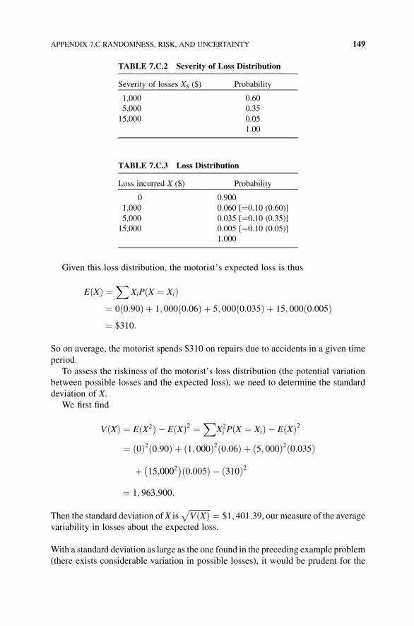
Given this loss distribution, the motorist’s expected loss is thus
EðXÞ ¼X
XiPðX ¼ XiÞ¼ 0ð0:90Þ þ 1; 000ð0:06Þ þ 5; 000ð0:035Þ þ 15; 000ð0:005Þ¼ $310:
So on average, the motorist spends $310 on repairs due to accidents in a given time
period.
To assess the riskiness of the motorist’s loss distribution (the potential variation
between possible losses and the expected loss), we need to determine the standard
deviation of X.
We first find
VðXÞ ¼ EðX2Þ � EðXÞ2 ¼X
X2i P X ¼ Xið Þ � EðXÞ2
¼ 0ð Þ2 0:90ð Þ þ 1; 000ð Þ2 0:06ð Þ þ 5; 000ð Þ2 0:035ð Þ
þ 15;0002� �
0:005ð Þ � 310ð Þ2
¼ 1; 963;900:
Then the standard deviation of X isffiffiffiffiffiffiffiffiffiffiffiVðXÞp ¼ $1; 401:39, our measure of the average
variability in losses about the expected loss.
With a standard deviation as large as the one found in the preceding example problem
(there exists considerable variation in possible losses), it would be prudent for the
TABLE 7.C.2 Severity of Loss Distribution
Severity of losses XS ($) Probability
1,000 0.60
5,000 0.35
15,000 0.05
1.00
TABLE 7.C.3 Loss Distribution
Loss incurred X ($) Probability
0 0.900
1,000 0.060 [¼0.10 (0.60)]
5,000 0.035 [¼0.10 (0.35)]
15,000 0.005 [¼0.10 (0.05)]
1.000
APPENDIX 7.C RANDOMNESS, RISK, AND UNCERTAINTY 149
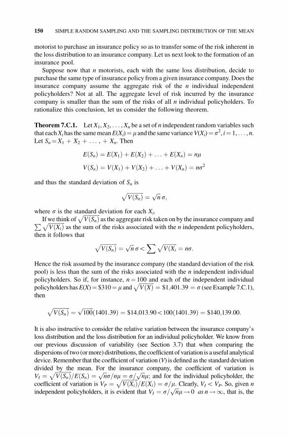
motorist to purchase an insurance policy so as to transfer some of the risk inherent in
the loss distribution to an insurance company. Let us next look to the formation of an
insurance pool.
Suppose now that n motorists, each with the same loss distribution, decide to
purchase the same type of insurance policy from a given insurance company. Does the
insurance company assume the aggregate risk of the n individual independent
policyholders? Not at all. The aggregate level of risk incurred by the insurance
company is smaller than the sum of the risks of all n individual policyholders. To
rationalize this conclusion, let us consider the following theorem.
Theorem 7.C.1. Let X1,X2, . . . ,Xn be a set of n independent random variables such
that eachXi has the samemeanE(Xi)¼ m and the samevarianceV(Xi)¼ s2, i¼ 1, . . . ,n.Let Sn¼X1 þ X2 þ . . . , þ Xn. Then
E Snð Þ ¼ E X1ð Þ þ E X2ð Þ þ . . .þ E Xnð Þ ¼ nm
V Snð Þ ¼ V X1ð Þ þ V X2ð Þ þ . . .þ V Xnð Þ ¼ ns2
and thus the standard deviation of Sn is
ffiffiffiffiffiffiffiffiffiffiffiffiVðSnÞ
p¼ ffiffiffi
np
s;
where s is the standard deviation for each Xi.
If we think offfiffiffiffiffiffiffiffiffiffiffiffiVðSnÞ
pas the aggregate risk taken on by the insurance company andP ffiffiffiffiffiffiffiffiffiffiffiffi
V Xið Þpas the sum of the risks associated with the n independent policyholders,
then it follows that
ffiffiffiffiffiffiffiffiffiffiffiffiVðSnÞ
p¼ ffiffiffi
np
sGX ffiffiffiffiffiffiffiffiffiffi
VðXi
p¼ ns:
Hence the risk assumed by the insurance company (the standard deviation of the risk
pool) is less than the sum of the risks associated with the n independent individual
policyholders. So if, for instance, n¼ 100 and each of the independent individual
policyholders hasE(X)¼ $310¼ m andffiffiffiffiffiffiffiffiffiffiffiVðXÞp ¼ $1;401:39 ¼ s (see Example 7.C.1),
then
ffiffiffiffiffiffiffiffiffiffiffiffiV Snð Þ
p¼
ffiffiffiffiffiffiffiffi100
p1401:39ð Þ ¼ $14;013:90G100ð1401:39Þ ¼ $140;139:00:
It is also instructive to consider the relative variation between the insurance company’s
loss distribution and the loss distribution for an individual policyholder. We know from
our previous discussion of variability (see Section 3.7) that when comparing the
dispersions of two (ormore) distributions, the coefficient of variation is a useful analytical
device. Remember that the coefficient of variation (V) is defined as the standard deviation
divided by the mean. For the insurance company, the coefficient of variation is
VI ¼ffiffiffiffiffiffiffiffiffiffiffiffiVðSnÞ
p=E Snð Þ ¼ ffiffiffi
np
s=nm ¼ s=ffiffiffin
pm; and for the individual policyholder, the
coefficient of variation is VP ¼ ffiffiffiffiffiffiffiffiffiffiffiffiV Xið Þp
=E Xið Þ ¼ s=m: Clearly, VIGVP. So, given n
independent policyholders, it is evident that VI ¼ s=ffiffiffin
pm! 0 as n!1, that is, the
150 SIMPLE RANDOM SAMPLING AND THE SAMPLING DISTRIBUTION OF THE MEAN

insurance company’s relative risk, as indexed by the coefficient of variation, approaches
zero as the size of the risk pool increases without bound. Clearly, large pools of
independent and similarly situated customers are preferred by the company to small
ones. In terms of the results obtained in Example 7.C.1,
VI ¼ffiffiffiffiffiffiffiffiffiffiffiffiV Snð Þp
E Snð Þ � 100 ¼ sffiffiffin
pm� 100 ¼ 1403:39ffiffiffiffiffiffiffiffi
100p ð300Þ � 100 ¼ 45:2%
VP ¼ffiffiffiffiffiffiffiffiffiffiffiffiV Xið Þp
E Xið Þ � 100 ¼ sm� 100 ¼ 1403:39
310� 100 ¼ 452:1%:
So for the insurance company, the standard deviation is 45.2% of the mean; for anindividual customer, the standard deviation is 452.1% of the mean. Thus there ismuch less risk associated with the insurance company's loss distribution relative tothat for a given policyholder.
APPENDIX 7.C RANDOMNESS, RISK, AND UNCERTAINTY 151
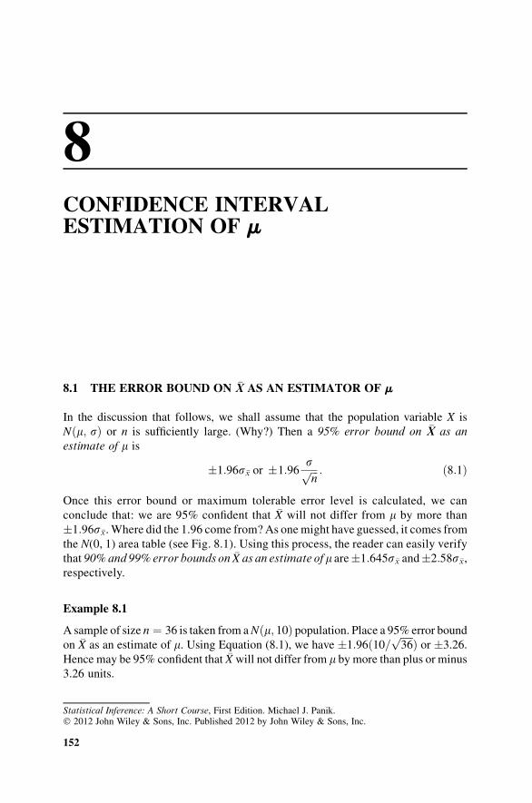
8CONFIDENCE INTERVALESTIMATION OF m
8.1 THE ERROR BOUND ON �X AS AN ESTIMATOR OF m
In the discussion that follows, we shall assume that the population variable X is
Nðm; sÞ or n is sufficiently large. (Why?) Then a 95% error bound on �X as an
estimate of m is
�1:96s�x or �1:96sffiffiffin
p : ð8:1Þ
Once this error bound or maximum tolerable error level is calculated, we can
conclude that: we are 95% confident that �X will not differ from m by more than
�1:96s�x. Where did the 1.96 come from?As onemight have guessed, it comes from
the N(0, 1) area table (see Fig. 8.1). Using this process, the reader can easily verify
that 90%and 99% error bounds on �X as an estimate of m are�1:645s�x and�2:58s�x,
respectively.
Example 8.1
A sample of size n ¼ 36 is taken from aNðm; 10Þ population. Place a 95% error bound
on �X as an estimate of m. Using Equation (8.1), we have �1:96ð10= ffiffiffiffiffi36
p Þ or �3.26.
Hence may be 95% confident that �X will not differ from m by more than plus or minus
3.26 units.
Statistical Inference: A Short Course, First Edition. Michael J. Panik.� 2012 John Wiley & Sons, Inc. Published 2012 by John Wiley & Sons, Inc.
152
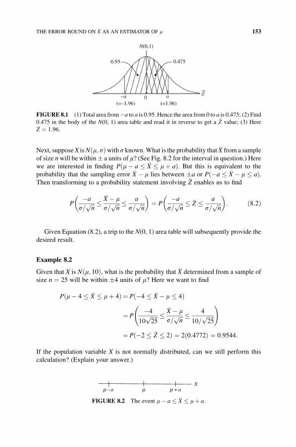
Next, supposeX isNðm; sÞwith s known.What is the probability that �X from a sample
of size nwill be within� a units of m? (See Fig. 8.2 for the interval in question.) Herewe are interested in finding Pðm� a � �X � mþ aÞ. But this is equivalent to the
probability that the sampling error �X � m lies between �a or Pð�a � �X � m � aÞ.Then transforming to a probability statement involving �Z enables us to find
P�a
s=ffiffiffin
p ��X � ms=
ffiffiffin
p � a
s=ffiffiffin
p� �
¼ P�a
s=ffiffiffin
p � �Z � a
s=ffiffiffin
p� �
: ð8:2Þ
Given Equation (8.2), a trip to the N(0, 1) area table will subsequently provide the
desired result.
Example 8.2
Given that X is Nðm; 10Þ, what is the probability that �X determined from a sample of
size n ¼ 25 will be within �4 units of m? Here we want to find
Pðm� 4 � �X � mþ 4Þ ¼ Pð�4 � �X � m � 4Þ
¼ P�4
10ffiffiffiffiffi25
p ��X � ms=
ffiffiffin
p � 4
10=ffiffiffiffiffi25
p !
¼ Pð�2 � �Z � 2Þ ¼ 2ð0:4772Þ ¼ 0:9544:
If the population variable X is not normally distributed, can we still perform this
calculation? (Explain your answer.)
FIGURE 8.1 (1) Total area from�a to a is 0.95. Hence the area from 0 to a is 0.475; (2) Find
0.475 in the body of the N(0, 1) area table and read it in reverse to get a �Z value; (3) Here�Z ¼ 1:96.
X μ – a μ + a μ
FIGURE 8.2 The event m� a � �X � mþ a.
THE ERROR BOUND ON �X AS AN ESTIMATOR OF m 153
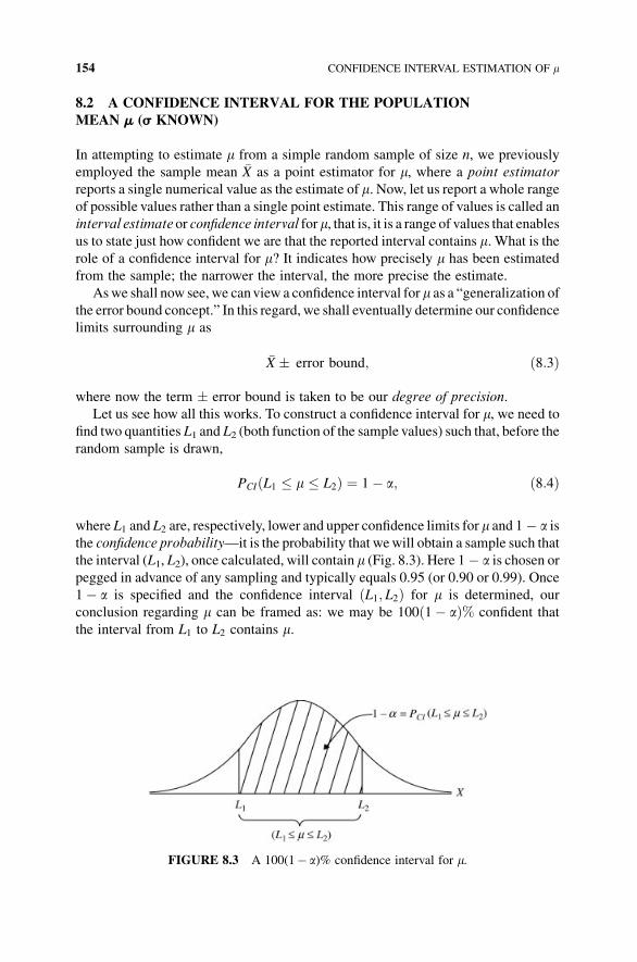
8.2 A CONFIDENCE INTERVAL FOR THE POPULATION
MEAN m (s KNOWN)
In attempting to estimate m from a simple random sample of size n, we previously
employed the sample mean �X as a point estimator for m, where a point estimator
reports a single numerical value as the estimate of m. Now, let us report a whole rangeof possible values rather than a single point estimate. This range of values is called an
interval estimate or confidence interval form, that is, it is a range of values that enablesus to state just how confident we are that the reported interval contains m. What is the
role of a confidence interval for m? It indicates how precisely m has been estimated
from the sample; the narrower the interval, the more precise the estimate.
Aswe shall now see, we canview a confidence interval for m as a “generalization ofthe error bound concept.” In this regard, we shall eventually determine our confidence
limits surrounding m as
�X � error bound; ð8:3Þ
where now the term � error bound is taken to be our degree of precision.
Let us see how all this works. To construct a confidence interval for m, we need tofind two quantities L1 and L2 (both function of the sample values) such that, before the
random sample is drawn,
PCI L1 � m � L2ð Þ ¼ 1� a; ð8:4Þ
where L1 and L2 are, respectively, lower and upper confidence limits for m and 1� a isthe confidence probability—it is the probability that wewill obtain a sample such that
the interval (L1, L2), once calculated, will contain m (Fig. 8.3). Here 1� a is chosen orpegged in advance of any sampling and typically equals 0.95 (or 0.90 or 0.99). Once
1� a is specified and the confidence interval ðL1; L2Þ for m is determined, our
conclusion regarding m can be framed as: we may be 100ð1� aÞ% confident that
the interval from L1 to L2 contains m.
FIGURE 8.3 A 100(1� a)% confidence interval for m.
154 CONFIDENCE INTERVAL ESTIMATION OF m
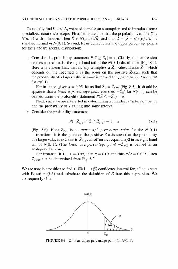
To actually find L1 and L2 we need to make an assumption and to introduce some
specialized notation/concepts. First, let us assume that the population variable X is
N(m, s) with s known. Then �X is Nðm; s= ffiffiffin
p Þ and thus �Z ¼ ð �X � mÞ=ðs= ffiffiffiffiffinÞp
is
standard normal or Nð0; 1Þ. Second, let us define lower and upper percentage points
for the standard normal distribution:
a. Consider the probability statement Pð�Z � �ZaÞ ¼ a. Clearly, this expression
defines an area under the right-hand tail of the Nð0; 1Þ distribution (Fig. 8.4).
Here a is chosen first, that is, any a implies a �Za value. Hence �Za, which
depends on the specified a, is the point on the positive �Z-axis such that
the probability of a larger value is a—it is termed an upper a percentage pointfor N(0,1).
For instance, given a ¼ 0:05, let us find �Za ¼ �Z0:05 (Fig. 8.5). It should be
apparent that a lower a percentage point (denoted ��Za) for Nð0; 1Þ can be
defined using the probability statement Pð�Z � ��ZaÞ ¼ a.Next, since we are interested in determining a confidence “interval,” let us
find the probability of �Z falling into some interval.
b. Consider the probability statement
Pð��Za=2 � �Z � �Za=2Þ ¼ 1� a ð8:5Þ(Fig. 8.6). Here �Za=2 is an upper a=2 percentage point for the Nð0; 1Þdistribution—it is the point on the positive �Z-axis such that the probability
of a larger value is a=2, that is, �Za=2 cuts off an area equal to a=2 in the right-handtail of N(0, 1). (The lower a=2 percentage point ��Za=2 is defined in an
analogous fashion.)
For instance, if 1� a ¼ 0:95, then a ¼ 0:05 and thus a=2 ¼ 0:025. Then�Z0:025 can be determined from Fig. 8.7.
We are now in a position to find a 100ð1� aÞ% confidence interval for m. Let us startwith Equation (8.5) and substitute the definition of �Z into this expression. We
consequently obtain:
FIGURE 8.4 �Za is an upper percentage point for N(0, 1).
A CONFIDENCE INTERVAL FOR THE POPULATION MEAN m (s KNOWN) 155
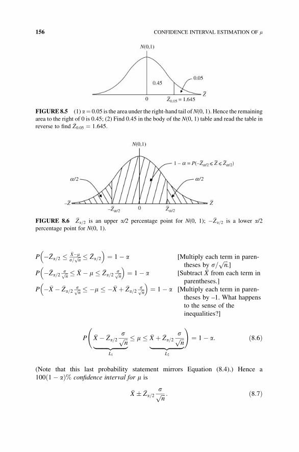
P ��Za=2 � �X�ms=ffiffin
p � �Za=2
� �¼ 1� a [Multiply each term in paren-
theses by s=ffiffiffin
p.]
P ��Za=2sffiffin
p � �X � m � �Za=2sffiffin
p� �
¼ 1� a [Subtract �X from each term in
parentheses.]
P � �X � �Za=2sffiffin
p � �m � � �X þ �Za=2sffiffin
p� �
¼ 1� a [Multiply each term in paren-
theses by –1. What happens
to the sense of the
inequalities?]
P
�X � �Za=2
sffiffiffin
p|fflfflfflfflfflfflfflffl{zfflfflfflfflfflfflfflffl}
L1
� m � �X þ �Za=2sffiffiffin
p|fflfflfflfflfflfflfflffl{zfflfflfflfflfflfflfflffl}
L2
!¼ 1� a: ð8:6Þ
(Note that this last probability statement mirrors Equation (8.4).) Hence a
100ð1� aÞ% confidence interval for m is
�X � �Za=2sffiffiffin
p : ð8:7Þ
FIGURE8.5 (1) a¼ 0.05 is the area under the right-hand tail ofN(0, 1). Hence the remaining
area to the right of 0 is 0.45; (2) Find 0.45 in the body of the N(0, 1) table and read the table in
reverse to find �Z0:05 ¼ 1:645:
FIGURE 8.6 �Za=2 is an upper a/2 percentage point for N(0, 1); ��Za=2 is a lower a/2percentage point for N(0, 1).
156 CONFIDENCE INTERVAL ESTIMATION OF m
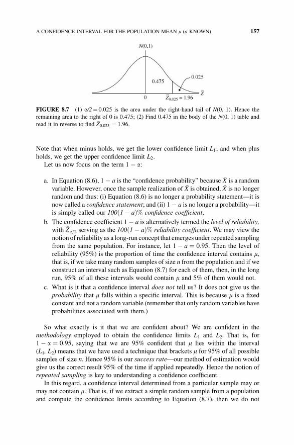
Note that when minus holds, we get the lower confidence limit L1; and when plus
holds, we get the upper confidence limit L2.
Let us now focus on the term 1� a:
a. In Equation (8.6), 1� a is the “confidence probability” because �X is a random
variable. However, once the sample realization of �X is obtained, �X is no longer
random and thus: (i) Equation (8.6) is no longer a probability statement—it is
now called a confidence statement; and (ii) 1� a is no longer a probability—it
is simply called our 100ð1� aÞ% confidence coefficient.
b. The confidence coefficient 1� a is alternatively termed the level of reliability,
with �Za=2 serving as the 100ð1� aÞ% reliability coefficient. We may view the
notion of reliability as a long-run concept that emerges under repeated sampling
from the same population. For instance, let 1� a ¼ 0:95. Then the level of
reliability (95%) is the proportion of time the confidence interval contains m,that is, if we take many random samples of size n from the population and if we
construct an interval such as Equation (8.7) for each of them, then, in the long
run, 95% of all these intervals would contain m and 5% of them would not.
c. What is it that a confidence interval does not tell us? It does not give us the
probability that m falls within a specific interval. This is because m is a fixed
constant and not a random variable (remember that only random variables have
probabilities associated with them.)
So what exactly is it that we are confident about? We are confident in the
methodology employed to obtain the confidence limits L1 and L2. That is, for
1� a ¼ 0:95, saying that we are 95% confident that m lies within the interval
(L1, L2) means that we have used a technique that brackets m for 95% of all possible
samples of size n. Hence 95% is our success rate—our method of estimation would
give us the correct result 95% of the time if applied repeatedly. Hence the notion of
repeated sampling is key to understanding a confidence coefficient.
In this regard, a confidence interval determined from a particular sample may or
may not contain m. That is, if we extract a simple random sample from a population
and compute the confidence limits according to Equation (8.7), then we do not
FIGURE 8.7 (1) a/2¼ 0.025 is the area under the right-hand tail of N(0, 1). Hence the
remaining area to the right of 0 is 0.475; (2) Find 0.475 in the body of the N(0, 1) table and
read it in reverse to find �Z0:025 ¼ 1:96.
A CONFIDENCE INTERVAL FOR THE POPULATION MEAN m (s KNOWN) 157
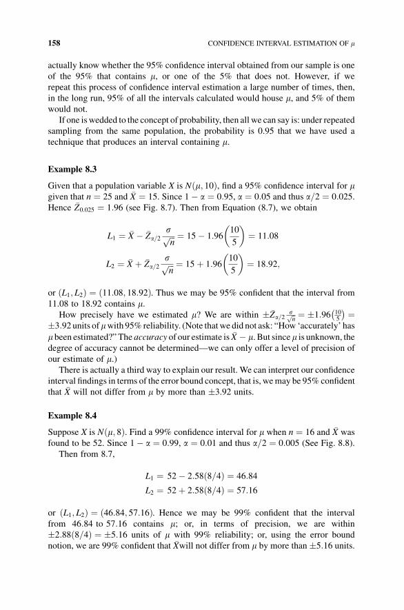
actually know whether the 95% confidence interval obtained from our sample is one
of the 95% that contains m, or one of the 5% that does not. However, if we
repeat this process of confidence interval estimation a large number of times, then,
in the long run, 95% of all the intervals calculated would house m, and 5% of them
would not.
If one is wedded to the concept of probability, then all we can say is: under repeated
sampling from the same population, the probability is 0.95 that we have used a
technique that produces an interval containing m.
Example 8.3
Given that a population variable X is Nðm; 10Þ, find a 95% confidence interval for mgiven that n ¼ 25 and �X ¼ 15. Since 1� a ¼ 0:95, a ¼ 0:05 and thus a=2 ¼ 0:025.Hence �Z0:025 ¼ 1:96 (see Fig. 8.7). Then from Equation (8.7), we obtain
L1 ¼ �X � �Za=2sffiffiffin
p ¼ 15� 1:9610
5
� �¼ 11:08
L2 ¼ �X þ �Za=2sffiffiffin
p ¼ 15þ 1:9610
5
� �¼ 18:92;
or ðL1; L2Þ ¼ ð11:08; 18:92Þ. Thus we may be 95% confident that the interval from
11.08 to 18.92 contains m.How precisely have we estimated m? We are within ��Za=2
sffiffin
p ¼ �1:96 105
� ¼�3:92 units ofmwith 95% reliability. (Note thatwe did not ask: “How ‘accurately’ has
m been estimated?” The accuracy of our estimate is �X � m. But sincem is unknown, thedegree of accuracy cannot be determined—we can only offer a level of precision of
our estimate of m.)There is actually a third way to explain our result. We can interpret our confidence
interval findings in terms of the error bound concept, that is, wemay be 95% confident
that �X will not differ from m by more than �3.92 units.
Example 8.4
Suppose X is Nðm; 8Þ. Find a 99% confidence interval for m when n ¼ 16 and �X was
found to be 52. Since 1� a ¼ 0:99, a ¼ 0:01 and thus a=2 ¼ 0:005 (See Fig. 8.8).
Then from 8.7,
L1 ¼ 52� 2:58ð8=4Þ ¼ 46:84
L2 ¼ 52þ 2:58ð8=4Þ ¼ 57:16
or ðL1; L2Þ ¼ ð46:84; 57:16Þ. Hence we may be 99% confident that the interval
from 46:84 to 57:16 contains m; or, in terms of precision, we are within
�2:88ð8=4Þ ¼ �5:16 units of m with 99% reliability; or, using the error bound
notion, we are 99% confident that �Xwill not differ from m by more than �5:16 units.
158 CONFIDENCE INTERVAL ESTIMATION OF m
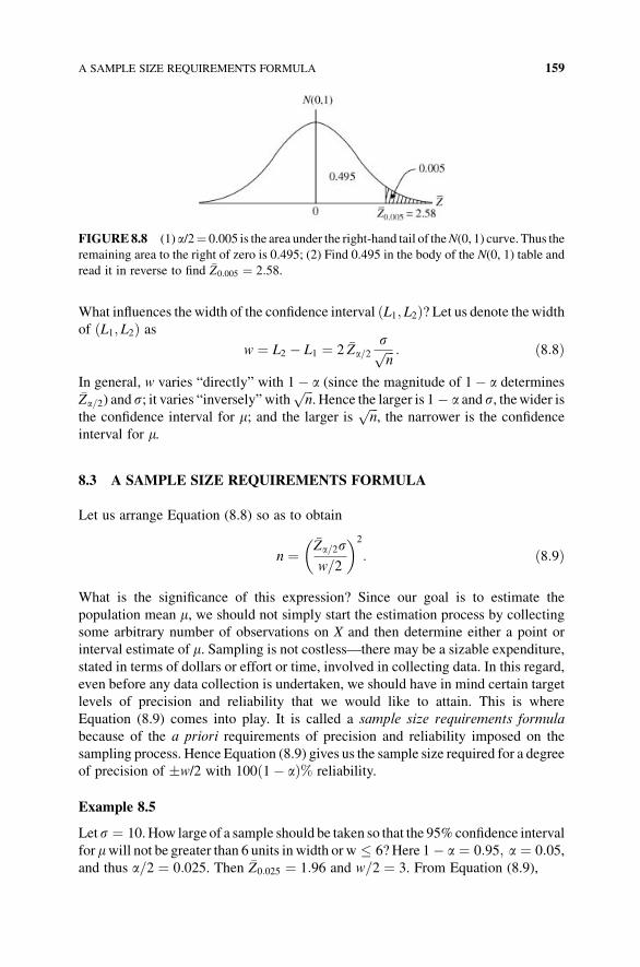
What influences thewidth of the confidence interval L1; L2ð Þ? Let us denote thewidthof L1; L2ð Þ as
w ¼ L2 � L1 ¼ 2 �Za=2sffiffiffin
p : ð8:8Þ
In general, w varies “directly” with 1� a (since the magnitude of 1� a determines�Za=2) and s; it varies “inversely” with
ffiffiffin
p. Hence the larger is 1� a and s, thewider is
the confidence interval for m; and the larger isffiffiffin
p, the narrower is the confidence
interval for m.
8.3 A SAMPLE SIZE REQUIREMENTS FORMULA
Let us arrange Equation (8.8) so as to obtain
n ¼�Za=2sw=2
� �2
: ð8:9Þ
What is the significance of this expression? Since our goal is to estimate the
population mean m, we should not simply start the estimation process by collecting
some arbitrary number of observations on X and then determine either a point or
interval estimate of m. Sampling is not costless—there may be a sizable expenditure,
stated in terms of dollars or effort or time, involved in collecting data. In this regard,
even before any data collection is undertaken, we should have in mind certain target
levels of precision and reliability that we would like to attain. This is where
Equation (8.9) comes into play. It is called a sample size requirements formula
because of the a priori requirements of precision and reliability imposed on the
sampling process. Hence Equation (8.9) gives us the sample size required for a degree
of precision of �w/2 with 100ð1� aÞ% reliability.
Example 8.5
Lets ¼ 10.How large of a sample should be taken so that the 95%confidence interval
for mwill not be greater than 6 units in width or w � 6?Here 1� a ¼ 0:95; a ¼ 0:05,and thus a=2 ¼ 0:025. Then �Z0:025 ¼ 1:96 and w=2 ¼ 3. From Equation (8.9),
FIGURE8.8 (1) a/2¼ 0.005 is the area under the right-hand tail of theN(0, 1) curve. Thus the
remaining area to the right of zero is 0.495; (2) Find 0.495 in the body of the N(0, 1) table and
read it in reverse to find �Z0:005 ¼ 2:58.
A SAMPLE SIZE REQUIREMENTS FORMULA 159
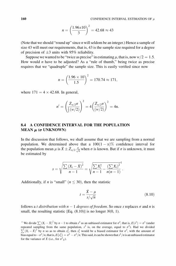
n ¼ 1:96x10
3
� �2
¼ 42:68 � 43
(Note that we should “round up” since nwill seldom be an integer.) Hence a sample of
size 43 will meet our requirements, that is, 43 is the sample size required for a degree
of precision of �3 units with 95% reliability.
Supposewewanted to be “twice as precise” in estimatingm, that is, noww=2 ¼ 1:5.How would n have to be adjusted? As a “rule of thumb,” being twice as precise
requires that we “quadruple” the sample size. This is easily verified since now
n ¼ 1:96� 10
1:5
� �2
¼ 170:74 � 171;
where 171 ¼ 4� 42:68. In general,
n0 ¼�Za=2s
12ðw=2Þ
!2
¼ 4�Za=2sðw=2Þ� �2
¼ 4n:
8.4 A CONFIDENCE INTERVAL FOR THE POPULATION
MEAN m (s UNKNOWN)
In the discussion that follows, we shall assume that we are sampling from a normal
population. We determined above that a 100ð1� aÞ% confidence interval for
the population mean m is �X � �Za=2sffiffin
p when s is known. But if s is unknown, it must
be estimated by
s ¼ffiffiffiffiffiffiffiffiffiffiffiffiffiffiffiffiffiffiffiffiffiffiffiffiffiP ðXi � �XÞ2
n� 1
s
¼ffiffiffiffiffiffiffiffiffiffiffiffiffiffiffiffiffiffiffiffiffiffiffiffiffiffiffiffiffiffiffiffiffiffiP
X2i
n� 1�P
Xið Þ2nðn� 1Þ
s 1
:
Additionally, if n is “small” ðn � 30Þ, then the statistic
t ¼�X � ms=
ffiffiffin
p ð8:10Þ
follows a t distribution with n� 1 degrees of freedom. So once s replaces s and n is
small, the resulting statistic [Eq. (8.10)] is no longer N(0, 1).
1 We divideP
Xi � �Xð Þ2 by n� 1 to obtain s2 as an unbiased estimator for s2, that is, E s2ð Þ ¼ s2 (underrepeated sampling from the same population, s2 is, on the average, equal to s2). Had we dividedP
Xi � �Xð Þ2 by n so as to obtain s21, then s21 would be a biased estimator for s2, with the amount of
bias equal to�s2=n, that is,E s21� ¼ s2 � s2=n. This said, it can be shown that s2=n is an unbiased estimator
for the variance of �X (i.e., for s2 �X).
160 CONFIDENCE INTERVAL ESTIMATION OF m
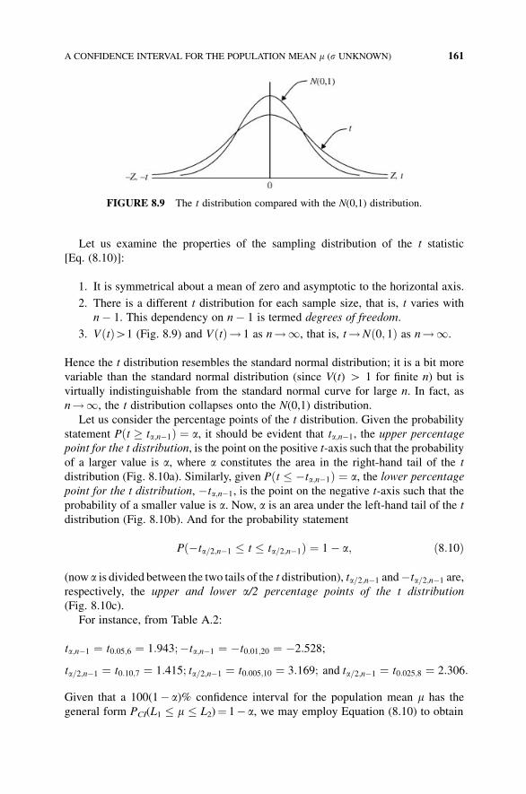
Let us examine the properties of the sampling distribution of the t statistic
[Eq. (8.10)]:
1. It is symmetrical about a mean of zero and asymptotic to the horizontal axis.
2. There is a different t distribution for each sample size, that is, t varies with
n� 1. This dependency on n� 1 is termed degrees of freedom.
3. VðtÞH1 (Fig. 8.9) and VðtÞ! 1 as n!1, that is, t!Nð0; 1Þ as n!1.
Hence the t distribution resembles the standard normal distribution; it is a bit more
variable than the standard normal distribution (since V(t) H 1 for finite n) but is
virtually indistinguishable from the standard normal curve for large n. In fact, as
n!1, the t distribution collapses onto the N(0,1) distribution.
Let us consider the percentage points of the t distribution. Given the probability
statement Pðt � ta;n�1Þ ¼ a, it should be evident that ta;n�1, the upper percentage
point for the t distribution, is the point on the positive t-axis such that the probability
of a larger value is a, where a constitutes the area in the right-hand tail of the t
distribution (Fig. 8.10a). Similarly, given Pðt � �ta;n�1Þ ¼ a, the lower percentagepoint for the t distribution, �ta;n�1, is the point on the negative t-axis such that the
probability of a smaller value is a. Now, a is an area under the left-hand tail of the t
distribution (Fig. 8.10b). And for the probability statement
Pð�ta=2;n�1 � t � ta=2;n�1Þ ¼ 1� a; ð8:10Þ
(now a is divided between the two tails of the t distribution), ta=2;n�1 and�ta=2;n�1 are,
respectively, the upper and lower a/2 percentage points of the t distribution
(Fig. 8.10c).
For instance, from Table A.2:
ta;n�1 ¼ t0:05;6 ¼ 1:943;�ta;n�1 ¼ �t0:01;20 ¼ �2:528;
ta=2;n�1 ¼ t0:10;7 ¼ 1:415; ta=2;n�1 ¼ t0:005;10 ¼ 3:169; and ta=2;n�1 ¼ t0:025;8 ¼ 2:306:
Given that a 100(1� a)% confidence interval for the population mean m has the
general form PCI(L1 � m � L2)¼ 1� a, we may employ Equation (8.10) to obtain
FIGURE 8.9 The t distribution compared with the N(0,1) distribution.
A CONFIDENCE INTERVAL FOR THE POPULATION MEAN m (s UNKNOWN) 161
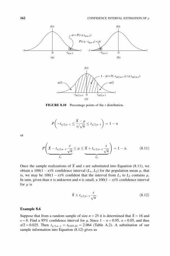
P �ta=2;n�1 ��X � ms=
ffiffiffin
p � ta=2;n�1
� �¼ 1� a
or
P
�X � ta=2;n�1
sffiffiffin
p|fflfflfflfflfflfflfflfflfflfflffl{zfflfflfflfflfflfflfflfflfflfflffl}
L1
� m � �X þ ta=2;n�1
sffiffiffin
p|fflfflfflfflfflfflfflfflfflfflffl{zfflfflfflfflfflfflfflfflfflfflffl}
L2
!¼ 1� a: ð8:11Þ
Once the sample realizations of �X and s are substituted into Equation (8.11), we
obtain a 100(1� a)% confidence interval (L1, L2) for the population mean m, thatis, we may be 100(1� a)% confident that the interval from L1 to L2 contains m.In sum, given than s is unknown and n is small, a 100(1� a)% confidence interval
for m is
�X � ta=2;n�1
sffiffiffin
p : ð8:12Þ
Example 8.6
Suppose that from a random sample of size n¼ 25 it is determined that �X¼ 16 and
s¼ 8. Find a 95% confidence interval for m. Since 1� a¼ 0.95, a¼ 0.05, and thus
a/2¼ 0.025. Then ta=2;n�1 ¼ t0:025;24 ¼ 2:064 (Table A.2). A substitution of our
sample information into Equation (8.12) gives us
FIGURE 8.10 Percentage points of the t distribution.
162 CONFIDENCE INTERVAL ESTIMATION OF m
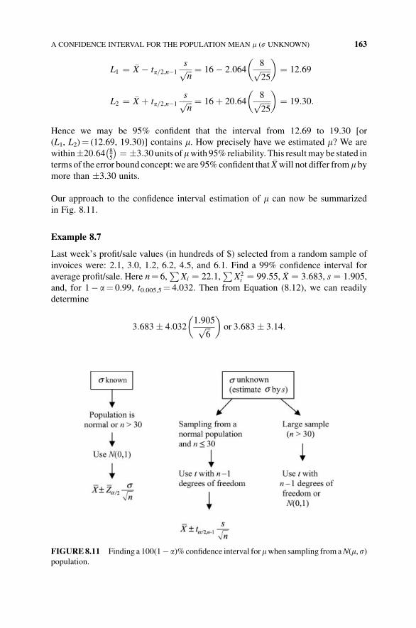
L1 ¼ �X � ta=2;n�1
sffiffiffin
p ¼ 16� 2:0648ffiffiffiffiffi25
p� �
¼ 12:69
L2 ¼ �X þ ta=2;n�1
sffiffiffin
p ¼ 16þ 20:648ffiffiffiffiffi25
p� �
¼ 19:30:
Hence we may be 95% confident that the interval from 12.69 to 19.30 [or
(L1, L2)¼ (12.69, 19.30)] contains m. How precisely have we estimated m? We are
within�20:64 85
� ¼ �3:30units ofmwith 95% reliability. This resultmay be stated in
terms of the error bound concept: we are 95%confident that �Xwill not differ from m bymore than �3.30 units.
Our approach to the confidence interval estimation of m can now be summarized
in Fig. 8.11.
Example 8.7
Last week’s profit/sale values (in hundreds of $) selected from a random sample of
invoices were: 2.1, 3.0, 1.2, 6.2, 4.5, and 6.1. Find a 99% confidence interval for
average profit/sale. Here n¼ 6,P
Xi ¼ 22:1,P
X2i ¼ 99:55, �X ¼ 3:683, s ¼ 1:905,
and, for 1� a¼ 0.99, t0.005,5¼ 4.032. Then from Equation (8.12), we can readily
determine
3:683� 4:0321:905ffiffiffi
6p
� �or 3:683� 3:14:
FIGURE8.11 Finding a 100(1� a)% confidence interval formwhen sampling fromaN(m,s)population.
A CONFIDENCE INTERVAL FOR THE POPULATION MEAN m (s UNKNOWN) 163
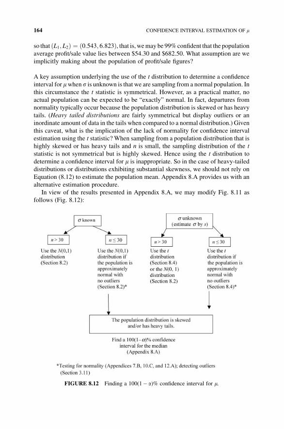
so that ðL1; L2Þ ¼ ð0:543; 6:823Þ, that is, wemay be 99%confident that the population
average profit/sale value lies between $54.30 and $682.50. What assumption are we
implicitly making about the population of profit/sale figures?
A key assumption underlying the use of the t distribution to determine a confidence
interval for mwhen s is unknown is that we are sampling from a normal population. In
this circumstance the t statistic is symmetrical. However, as a practical matter, no
actual population can be expected to be “exactly” normal. In fact, departures from
normality typically occur because the population distribution is skewed or has heavy
tails. (Heavy tailed distributions are fairly symmetrical but display outliers or an
inordinate amount of data in the tails when compared to a normal distribution.) Given
this caveat, what is the implication of the lack of normality for confidence interval
estimation using the t statistic? When sampling from a population distribution that is
highly skewed or has heavy tails and n is small, the sampling distribution of the t
statistic is not symmetrical but is highly skewed. Hence using the t distribution to
determine a confidence interval for m is inappropriate. So in the case of heavy-tailed
distributions or distributions exhibiting substantial skewness, we should not rely on
Equation (8.12) to estimate the population mean. Appendix 8.A provides us with an
alternative estimation procedure.
In view of the results presented in Appendix 8.A, we may modify Fig. 8.11 as
follows (Fig. 8.12):
FIGURE 8.12 Finding a 100(1� a)% confidence interval for m.
164 CONFIDENCE INTERVAL ESTIMATION OF m
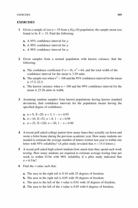
EXERCISES
1 Given a sample of size n¼ 35 from a N(m,10) population, the sample mean was
found to be �X ¼ 15. Find the following:
a. A 95% confidence interval for mb. A 90% confidence interval for mc. A 99% confidence interval for m
2 Given samples from a normal population with known variance, find the
following:
a. The confidence coefficient if n¼ 16, s2¼ 64, and the total width of the
confidence interval for the mean is 3.29 units.
b. The sample sizewhen s2¼ 100 and the 95% confidence interval for the mean
is 17.5–22.5.
c. The known variance when n¼ 100 and the 99% confidence interval for the
mean is 23.26 units in width.
3 Assuming random samples from known populations having known standard
deviations, find confidence intervals for the population means having the
specified degree of confidence:
a. n¼ 9, �X¼20, s¼ 3, 1� a¼ 0.95
b. n¼ 16, �X¼52, s¼ 8, 1� a¼ 0.99
c. n¼ 25, �X¼120, s¼ 20, 1� a¼ 0.90
4 A recent poll asked college juniors how many times they actually sat down and
wrote a letter home during the previous academic year. How many students are
needed to estimate the average number of letters written last year to within one
letter with 95% reliability? (A pilot study revealed that s¼ 15.4 letters.)
5 A recent poll asked high school students how much time they spend each week
texting. How many students are required to estimate average texting time per
week to within 0.5 hr with 90% reliability if a pilot study indicated that
s¼ 6.5 hr?
6 Find the t-value such that:
a. The area in the right tail is 0.10 with 25 degrees of freedom.
b. The area in the right tail is 0.05 with 30 degrees of freedom.
c. The area to the left of the t-value is 0.01 with 18 degrees of freedom.
d. The area to the left of the t-value is 0.05 with 6 degrees of freedom.
EXERCISES 165
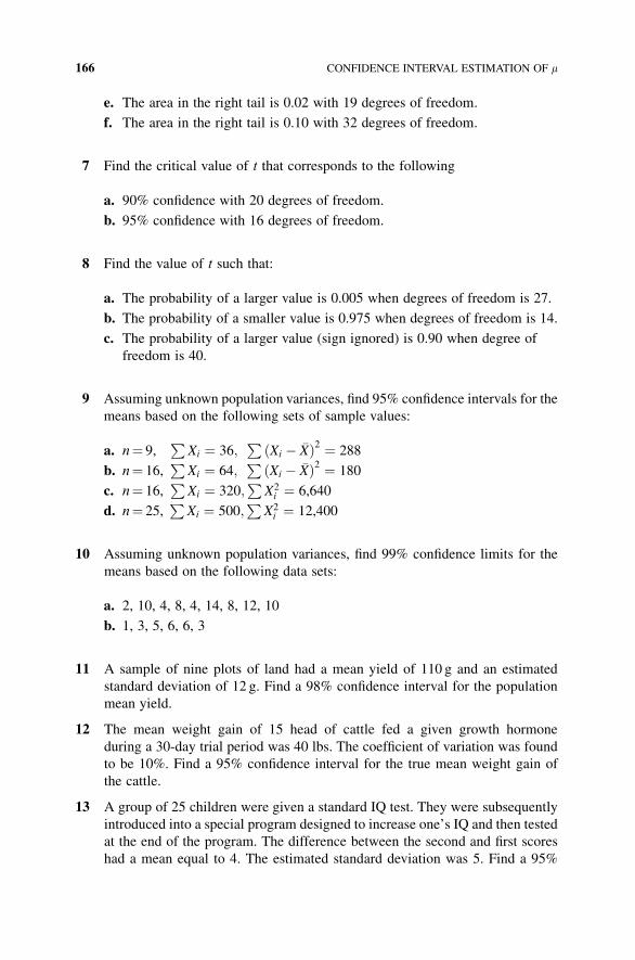
e. The area in the right tail is 0.02 with 19 degrees of freedom.
f. The area in the right tail is 0.10 with 32 degrees of freedom.
7 Find the critical value of t that corresponds to the following
a. 90% confidence with 20 degrees of freedom.
b. 95% confidence with 16 degrees of freedom.
8 Find the value of t such that:
a. The probability of a larger value is 0.005 when degrees of freedom is 27.
b. The probability of a smaller value is 0.975 when degrees of freedom is 14.
c. The probability of a larger value (sign ignored) is 0.90 when degree of
freedom is 40.
9 Assuming unknown population variances, find 95% confidence intervals for the
means based on the following sets of sample values:
a. n¼ 9,P
Xi ¼ 36;P
Xi � �Xð Þ2 ¼ 288
b. n¼ 16,P
Xi ¼ 64;P
Xi � �Xð Þ2 ¼ 180
c. n¼ 16,P
Xi ¼ 320;P
X2i ¼ 6,640
d. n¼ 25,P
Xi ¼ 500;P
X2i ¼ 12,400
10 Assuming unknown population variances, find 99% confidence limits for the
means based on the following data sets:
a. 2, 10, 4, 8, 4, 14, 8, 12, 10
b. 1, 3, 5, 6, 6, 3
11 A sample of nine plots of land had a mean yield of 110 g and an estimated
standard deviation of 12 g. Find a 98% confidence interval for the population
mean yield.
12 The mean weight gain of 15 head of cattle fed a given growth hormone
during a 30-day trial period was 40 lbs. The coefficient of variation was found
to be 10%. Find a 95% confidence interval for the true mean weight gain of
the cattle.
13 A group of 25 children were given a standard IQ test. They were subsequently
introduced into a special program designed to increase one’s IQ and then tested
at the end of the program. The difference between the second and first scores
had a mean equal to 4. The estimated standard deviation was 5. Find a 95%
166 CONFIDENCE INTERVAL ESTIMATION OF m
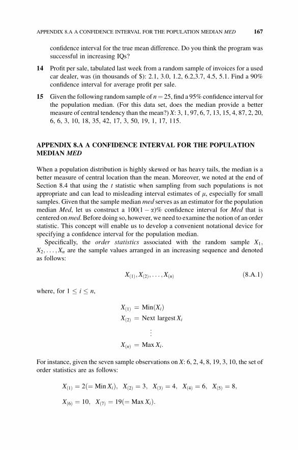
confidence interval for the true mean difference. Do you think the program was
successful in increasing IQs?
14 Profit per sale, tabulated last week from a random sample of invoices for a used
car dealer, was (in thousands of $): 2.1, 3.0, 1.2, 6.2,3.7, 4.5, 5.1. Find a 90%
confidence interval for average profit per sale.
15 Given the following random sample of n¼ 25, find a 95% confidence interval for
the population median. (For this data set, does the median provide a better
measure of central tendency than the mean?) X: 3, 1, 97, 6, 7, 13, 15, 4, 87, 2, 20,
6, 6, 3, 10, 18, 35, 42, 17, 3, 50, 19, 1, 17, 115.
APPENDIX 8.A A CONFIDENCE INTERVAL FOR THE POPULATION
MEDIAN MED
When a population distribution is highly skewed or has heavy tails, the median is a
better measure of central location than the mean. Moreover, we noted at the end of
Section 8.4 that using the t statistic when sampling from such populations is not
appropriate and can lead to misleading interval estimates of m, especially for small
samples. Given that the sample medianmed serves as an estimator for the population
median Med, let us construct a 100(1� a)% confidence interval for Med that is
centered onmed. Before doing so, however, we need to examine the notion of an order
statistic. This concept will enable us to develop a convenient notational device for
specifying a confidence interval for the population median.
Specifically, the order statistics associated with the random sample X1;X2; . . . ;Xn are the sample values arranged in an increasing sequence and denoted
as follows:
Xð1Þ;Xð2Þ; . . . ;XðnÞ ð8:A:1Þ
where, for 1 � i � n,
Xð1Þ ¼ MinðXiÞXð2Þ ¼ Next largest Xi
..
.
XðnÞ ¼ Max Xi:
For instance, given the seven sample observations on X: 6, 2, 4, 8, 19, 3, 10, the set of
order statistics are as follows:
Xð1Þ ¼ 2 ¼ Min Xið Þ; Xð2Þ ¼ 3; Xð3Þ ¼ 4; Xð4Þ ¼ 6; Xð5Þ ¼ 8;
Xð6Þ ¼ 10; Xð7Þ ¼ 19 ¼ Max Xið Þ:
APPENDIX 8.A A CONFIDENCE INTERVAL FOR THE POPULATION MEDIAN MED 167
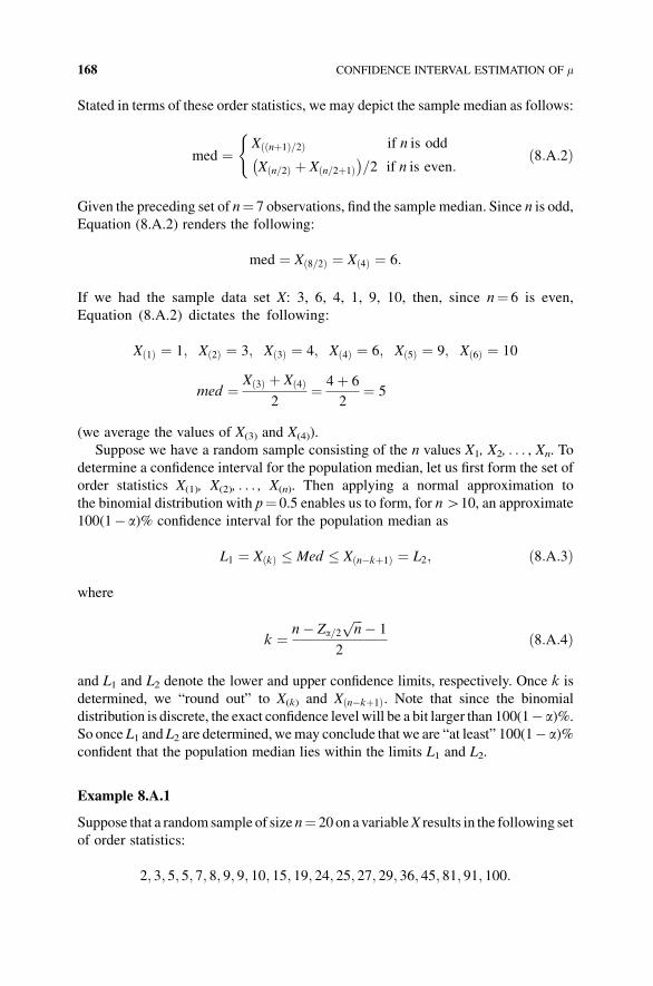
Stated in terms of these order statistics, we may depict the sample median as follows:
med ¼ Xððnþ1Þ=2Þ if n is odd
Xðn=2Þ þ Xðn=2þ1Þ�
=2 if n is even:
(ð8:A:2Þ
Given the preceding set of n¼ 7 observations, find the sample median. Since n is odd,
Equation (8.A.2) renders the following:
med ¼ Xð8=2Þ ¼ Xð4Þ ¼ 6:
If we had the sample data set X: 3, 6, 4, 1, 9, 10, then, since n¼ 6 is even,
Equation (8.A.2) dictates the following:
Xð1Þ ¼ 1; Xð2Þ ¼ 3; Xð3Þ ¼ 4; Xð4Þ ¼ 6; Xð5Þ ¼ 9; Xð6Þ ¼ 10
med ¼ Xð3Þ þ Xð4Þ2
¼ 4þ 6
2¼ 5
(we average the values of X(3) and X(4)).
Suppose we have a random sample consisting of the n values X1, X2, . . . , Xn. To
determine a confidence interval for the population median, let us first form the set of
order statistics X(1), X(2), . . . , X(n). Then applying a normal approximation to
the binomial distribution with p¼ 0.5 enables us to form, for nH10, an approximate
100(1� a)% confidence interval for the population median as
L1 ¼ XðkÞ � Med � Xðn�kþ1Þ ¼ L2; ð8:A:3Þ
where
k ¼ n� Za=2ffiffiffin
p � 1
2ð8:A:4Þ
and L1 and L2 denote the lower and upper confidence limits, respectively. Once k is
determined, we “round out” to X(k) and Xðn�kþ1Þ. Note that since the binomial
distribution is discrete, the exact confidence level will be a bit larger than 100(1� a)%.
So once L1 andL2 are determined, wemay conclude that we are “at least” 100(1� a)%confident that the population median lies within the limits L1 and L2.
Example 8.A.1
Suppose that a randomsample of size n¼ 20on avariableX results in the following set
of order statistics:
2; 3; 5; 5; 7; 8; 9; 9; 10; 15; 19; 24; 25; 27; 29; 36; 45; 81; 91; 100:
168 CONFIDENCE INTERVAL ESTIMATION OF m
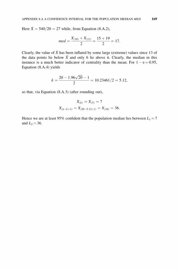
Here �X ¼ 540=20 ¼ 27 while, from Equation (8.A.2),
med ¼ Xð10Þ þ Xð11Þ2
¼ 15þ 19
2¼ 17:
Clearly, the value of �X has been inflated by some large (extreme) values since 13 of
the data points lie below �X and only 6 lie above it. Clearly, the median in this
instance is a much better indicator of centrality than the mean. For 1� a¼ 0.95,
Equation (8.A.4) yields
k ¼ 20� 1:96ffiffiffiffiffi20
p � 1
2¼ 10:23461=2 ¼ 5:12;
so that, via Equation (8.A.3) (after rounding out),
XðkÞ ¼ Xð5Þ ¼ 7
Xðn�kþ1Þ ¼ Xð20�5:12þ1Þ ¼ Xð16Þ ¼ 36:
Hence we are at least 95% confident that the population median lies between L1¼ 7
and L2¼ 36.
APPENDIX 8.A A CONFIDENCE INTERVAL FOR THE POPULATION MEDIAN MED 169
9THE SAMPLING DISTRIBUTION OF APROPORTION AND ITS CONFIDENCEINTERVAL ESTIMATION
9.1 THE SAMPLING DISTRIBUTION OF A PROPORTION
Our goal in this section is to estimate the parameter p of a binomial population.
Remember that a binomial population is one whose elements belong to either of two
classes—success or failure. Previously, the binomial random variable X was defined
as the number of successes obtained in n independent trials of a simple alternative
experiment and p denoted the probability of a success. Now, Xwill be taken to be the
number of successes observed in a simple random sample of size n and pwill represent
the proportion of successes in the population. (Obviously, 1� p is the population
proportion of failures.)
The problem that we now face is the estimation of p. Also, since we are basing our
estimate of p on sample information,we need to obtain some idea of the error involved
in estimating p. In order to adequately address these issues, we need to examine the
characteristics of the sampling distribution of the sample proportion. To this end, let us
extract a random sample of size n from a binomial population and find the observed
relative frequency of a success
p ¼ X
n¼ Observed number of success
n: ð9:1Þ
Statistical Inference: A Short Course, First Edition. Michael J. Panik.� 2012 John Wiley & Sons, Inc. Published 2012 by John Wiley & Sons, Inc.
170
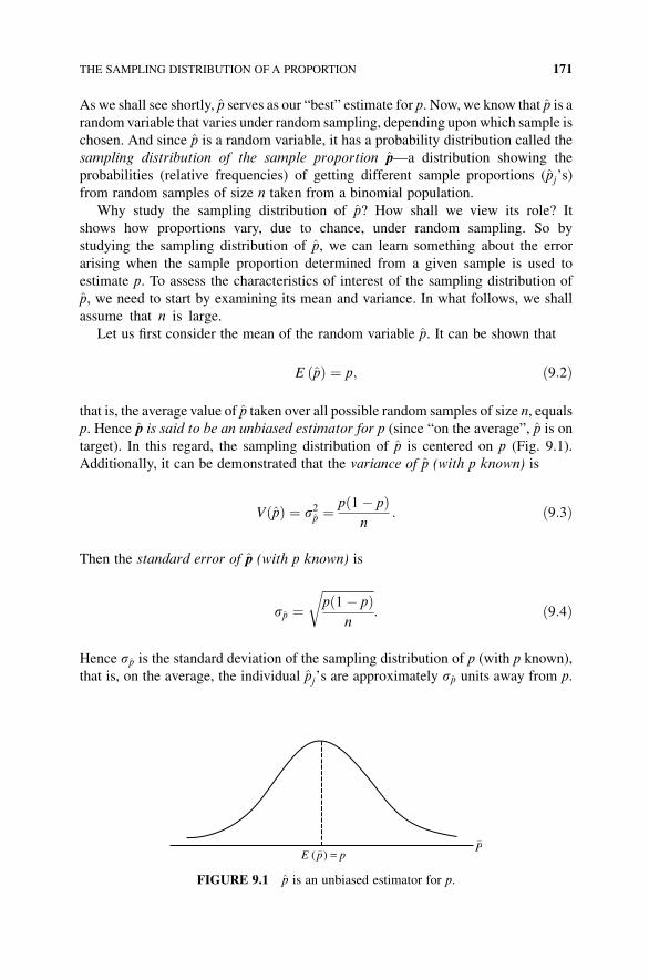
Aswe shall see shortly, p serves as our “best” estimate for p. Now, we know that p is a
random variable that varies under random sampling, depending uponwhich sample is
chosen. And since p is a random variable, it has a probability distribution called the
sampling distribution of the sample proportion p—a distribution showing the
probabilities (relative frequencies) of getting different sample proportions (pj’s)
from random samples of size n taken from a binomial population.
Why study the sampling distribution of p? How shall we view its role? It
shows how proportions vary, due to chance, under random sampling. So by
studying the sampling distribution of p, we can learn something about the error
arising when the sample proportion determined from a given sample is used to
estimate p. To assess the characteristics of interest of the sampling distribution of
p, we need to start by examining its mean and variance. In what follows, we shall
assume that n is large.
Let us first consider the mean of the random variable p. It can be shown that
E pð Þ ¼ p; ð9:2Þ
that is, the average value of p taken over all possible random samples of size n, equals
p. Hence p is said to be an unbiased estimator for p (since “on the average”, p is on
target). In this regard, the sampling distribution of p is centered on p (Fig. 9.1).
Additionally, it can be demonstrated that the variance of p (with p known) is
VðpÞ ¼ s2p ¼pð1� pÞ
n: ð9:3Þ
Then the standard error of p (with p known) is
sp ¼ffiffiffiffiffiffiffiffiffiffiffiffiffiffiffiffiffipð1� pÞ
n
r: ð9:4Þ
Hence sp is the standard deviation of the sampling distribution of p (with p known),
that is, on the average, the individual pj’s are approximately sp units away from p.
E (p) = pP
FIGURE 9.1 p is an unbiased estimator for p.
THE SAMPLING DISTRIBUTION OF A PROPORTION 171
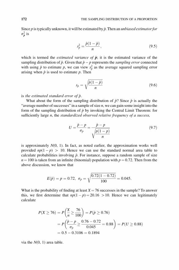
Since p is typically unknown, it will be estimated by p. Then an unbiased estimator for
s2p is
s2p ¼pð1� pÞ
n; ð9:5Þ
which is termed the estimated variance of p; it is the estimated variance of the
sampling distribution of p. Given that p� p represents the sampling error connected
with using p to estimate p, we can view s2p as the average squared sampling error
arising when p is used to estimate p. Then
sp ¼ffiffiffiffiffiffiffiffiffiffiffiffiffiffiffiffiffipð1� pÞ
n
rð9:6Þ
is the estimated standard error of p.
What about the form of the sampling distribution of p? Since p is actually the
“average number of successes” in a sample of size n, we can gain some insight into the
form of the sampling distribution of p by invoking the Central Limit Theorem: for
sufficiently large n, the standardized observed relative frequency of a success,
U ¼ p� p
sp¼ p� pffiffiffiffiffiffiffiffiffiffiffiffiffiffiffiffiffi
pð1� pÞn
r ð9:7Þ
is approximately N(0, 1). In fact, as noted earlier, the approximation works well
provided np(1� p) H 10. Hence we can use the standard normal area table to
calculate probabilities involving p. For instance, suppose a random sample of size
n¼ 100 is taken from an infinite (binomial) population with p¼ 0.72. Then from the
above discussion, we know that
EðpÞ ¼ p ¼ 0:72; sp ¼ffiffiffiffiffiffiffiffiffiffiffiffiffiffiffiffiffiffiffiffiffiffiffiffiffiffiffiffiffi0:72ð1� 0:72Þ
100
r¼ 0:045:
What is the probability of finding at least X¼ 76 successes in the sample? To answer
this, we first determine that np(1� p)¼ 20.16 H10. Hence we can legitimately
calculate
PðX � 76Þ ¼ PX
n� 76
100
� �¼ Pðp � 0:76Þ
¼ Pp� p
sp� 0:76� 0:72
0:045¼ 0:88
� �¼ PðU � 0:88Þ
¼ 0:5� 0:3106 ¼ 0:1894
via the N(0, 1) area table.
172 THE SAMPLING DISTRIBUTION OF A PROPORTION
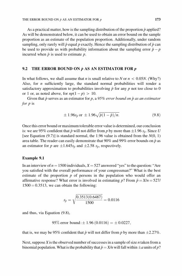
As a practical matter, how is the sampling distribution of the proportion p applied?
As will be demonstrated below, it can be used to obtain an error bound on the sample
proportion as an estimate of the population proportion. Additionally, under random
sampling, only rarely will p equal p exactly. Hence the sampling distribution of p can
be used to provide us with probability information about the sampling error p� p
incurred when p is used to estimate p.
9.2 THE ERROR BOUND ON p AS AN ESTIMATOR FOR p
In what follows, we shall assume that n is small relative to N or nG 0.05N. (Why?)
Also, for n sufficiently large, the standard normal probabilities will render a
satisfactory approximation to probabilities involving p for any p not too close to 0
or 1 or, as noted above, for np(1� p) H 10.
Given that p serves as an estimator for p, a 95% error bound on p as an estimator
for p is
� 1:96sp or � 1:96ffiffiffiffiffiffiffiffiffiffiffiffiffiffiffiffiffiffiffiffiffiffiffipð1� pÞ=n:
pð9:8Þ
Once this error bound ormaximum tolerable error value is determined, our conclusion
is: we are 95% confident that pwill not differ from p by more than�1.96 sp. SinceU
[see Equation (9.7)] is standard normal, the 1.96 value is obtained from the N(0, 1)
area table. The reader can easily demonstrate that 90% and 99% error bounds on p as
an estimator for p are �1.645sp and �2.58 sp, respectively.
Example 9.1
In an interview of n¼ 1500 individuals,X¼ 527 answered “yes” to the question: “Are
you satisfied with the overall performance of your congressman?” What is the best
estimate of the proportion p of persons in the population who would offer an
affirmative response? What error is involved in estimating p? From p¼X/n¼ 527/
1500¼ 0.3513, we can obtain the following:
sp ¼ffiffiffiffiffiffiffiffiffiffiffiffiffiffiffiffiffiffiffiffiffiffiffiffiffiffiffiffiffiffiffi0:3513ð0:6487Þ
1500
r¼ 0:0116
and thus, via Equation (9.8),
95% error bound :� 1:96 ð0:0116Þ ¼ � 0:0227;
that is, we may be 95% confident that p will not differ from p by more than�2.27%.
Next, supposeX is the observed number of successes in a sample of size n taken from a
binomial population.What is the probability that p¼X/nwill fall within�a units of p?
THE ERROR BOUND ON p AS AN ESTIMATOR FOR p 173
Here we are interested in finding P(p� a� p� p þ a). But this is equivalent to
the probability that the sampling error p� p lies between � a or P (�a� p� p� a).
Then transforming to a probability statement involving U enables us to find
P�a
sp� p� p
sp� a
sp
� �¼ P
�a
sp� U � a
sp
� �: ð9:9Þ
Example 9.2
What is the probability that p¼ 0.47 determined from a sample of size n¼ 250 taken
from a binomial population will be within �3% of p? Since
sp ¼ffiffiffiffiffiffiffiffiffiffiffiffiffiffiffiffiffiffiffiffiffi0:47ð0:53Þ
250
r¼ 0:032;
P p� 0:03 � p � pþ 0:03ð Þ ¼ P p� 0:03 � p � pþ 0:03ð Þ
¼ P�0:03
0:032� p� p
sp� 0:03
0:032
� �¼ P �0:94 � U � 0:94ð Þ
¼ 2ð0:3264Þ ¼ 0:6528:
9.3 A CONFIDENCE INTERVAL FOR THE POPULATION
PROPORTION (OF SUCCESSES) p
As an alternative to simply using p (determined from a simple random sample of size n
taken from a binomial population) as a point estimator for p, let us determine a whole
range of possible values that p could assume. This range of values is an interval
estimate or confidence interval for p, that is, it is a range of values that allows us to state
just how confident we are that the reported interval contains p. Once this interval is
obtained, it enables us to state just howprecisely phas been estimated from the sample;
the narrower the interval, the more precise the estimate.
As will be indicated below, a confidence interval “generalizes the error bound
concept.” In this regard, the confidence limits bounding p will be expressed as
p� error bound; ð9:10Þwhere the term � error bound serves as our degree of precision.
To construct a confidence interval for p, we need to find two quantities L1 and L2such that, before any sampling is undertaken,
PCIðL1 � p � L2Þ ¼ 1� a; ð9:11Þ
where L1 and L2 are lower and upper confidence limits for p, respectively, and 1� a isthe confidence probability, which is chosen in advance. Once 1� a is specified and L1
174 THE SAMPLING DISTRIBUTION OF A PROPORTION
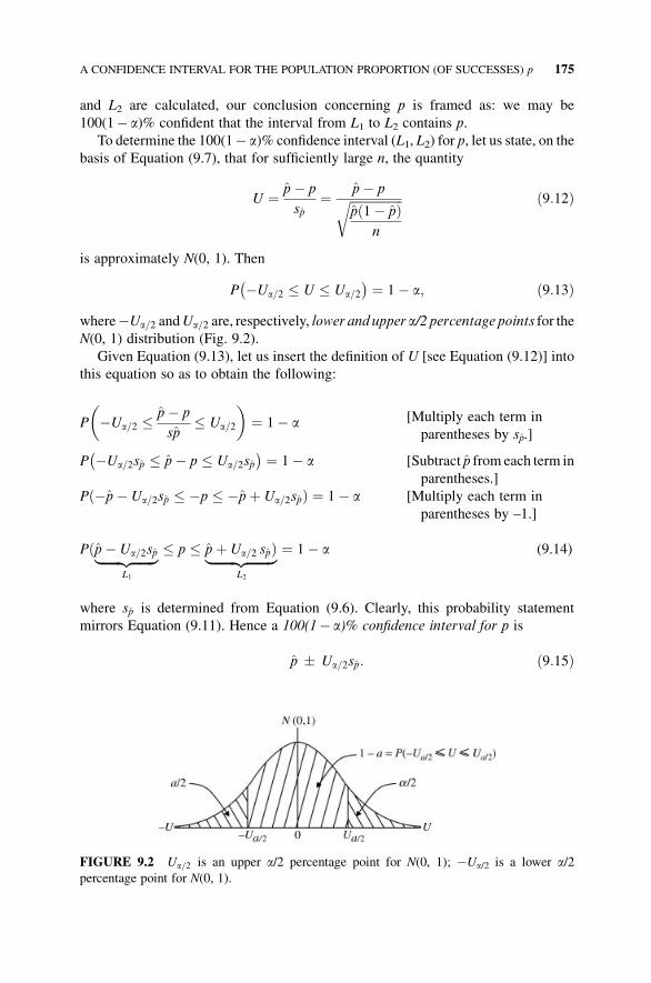
and L2 are calculated, our conclusion concerning p is framed as: we may be
100(1� a)% confident that the interval from L1 to L2 contains p.
To determine the 100(1� a)% confidence interval (L1, L2) for p, let us state, on the
basis of Equation (9.7), that for sufficiently large n, the quantity
U ¼ p� p
sp¼ p� pffiffiffiffiffiffiffiffiffiffiffiffiffiffiffiffiffi
pð1� pÞn
r ð9:12Þ
is approximately N(0, 1). Then
P �Ua=2 � U � Ua=2� � ¼ 1� a; ð9:13Þ
where�Ua=2 andUa=2 are, respectively, lower and upper a/2 percentage points for theN(0, 1) distribution (Fig. 9.2).
Given Equation (9.13), let us insert the definition of U [see Equation (9.12)] into
this equation so as to obtain the following:
P �Ua=2 � p� p
sp� Ua=2
� �¼ 1� a [Multiply each term in
parentheses by sp.]
P �Ua=2sp � p� p � Ua=2sp� � ¼ 1� a [Subtract p from each term in
parentheses.]
Pð�p� Ua=2sp � �p � �pþ Ua=2spÞ ¼ 1� a [Multiply each term in
parentheses by –1.]
Pðp� Ua=2sp|fflfflfflfflfflfflffl{zfflfflfflfflfflfflffl}L1
� p � pþ Ua=2 spÞ|fflfflfflfflfflfflfflffl{zfflfflfflfflfflfflfflffl}L2
¼ 1� a (9.14)
where sp is determined from Equation (9.6). Clearly, this probability statement
mirrors Equation (9.11). Hence a 100(1� a)% confidence interval for p is
p � Ua=2sp: ð9:15Þ
FIGURE 9.2 Ua=2 is an upper a/2 percentage point for N(0, 1); �Ua/2 is a lower a/2percentage point for N(0, 1).
A CONFIDENCE INTERVAL FOR THE POPULATION PROPORTION (OF SUCCESSES) p 175
So when minus holds, we get the lower confidence limit L1; and when plus holds, we
obtain the upper confidence limit L2.
In Equation (9.14) 1� a is a confidence probability since p is a random variable.
But once the sample realization of p is obtained (p is no longer random), 1� a is no
longer a probability—it is the 100(1� a)% confidence coefficient or level of reli-
ability, with Ua=2 serving as the 100(1� a)% reliability coefficient.
Example 9.3
Suppose that in a sample size of n¼ 100 it is found that X¼ 64 items display a
particular characteristic. Find a 95% confidence interval for p, the proportion of the
population having this characteristic. Here p ¼X/n¼ 0.64, sp ¼ ffiffiffiffiffiffiffiffiffiffiffiffiffiffiffiffiffiffiffiffiffiffiffip ð1� pÞ=np ¼
0.048, and 1� a¼ 0.95. Then a/2¼ 0.025 and, sinceU isN(0, 1),Ua=2¼U0:025¼ 1.96
(a review of Fig. 8.7 may be helpful). Then from Equation (9.15),
L1 ¼ p� Ua=2 sp ¼ 0:64� 1:96ð0:048Þ ¼ 0:546
L2 ¼ pþ Ua=2 sp ¼ 0:64þ 1:96ð0:048Þ ¼ 0:734:
Hence we may be 95% confident that the interval from 0.546 to 0.734 contains p.
How precisely have we estimated p? We are within �Ua=2 sp ¼ �1.96 (0.048)¼�0.094 or �9.4% of p with 95% reliability. Alternatively, we can invoke the error
bound concept and conclude that we are 95% confident that pwill not differ from p by
more than � 9.4%.
What influences the width of the confidence interval for p? From Equation (9.15),
w ¼ L2 � L1 ¼ 2Ua=2
ffiffiffiffiffiffiffiffiffiffiffiffiffiffiffiffiffipð1� pÞ
n
r: ð9:16Þ
Thus w varies “directly” with 1� a (since the size of 1� a determines Ua=2); it
varies “inversely” withffiffiffin
p. So the larger is 1� a, the wider is (L1, L2); and the larger
isffiffiffin
p, the narrower is (L1, L2).
9.4 A SAMPLE SIZE REQUIREMENTS FORMULA
Given Equation (9.16), let us solve for n or
n ¼ ðUa=2Þ2pð1� pÞðw=2Þ2 : ð9:17Þ
Let us refer to this expression as the sample size requirements formula. What are the
requirements? As noted above when employing Equation (8.9), they are “precision”
176 THE SAMPLING DISTRIBUTION OF A PROPORTION
and “reliability.” Hence Equation (9.17) provides us with the sample size required for
a degree of precision of �w/2 with 100(1� a)% reliability. (Note that w/2 should
always be expressed as a decimal.)
Example 9.4
Suppose we would like to estimate the proportion of individuals with a particular
characteristic towithin�3% of p (the population proportion of individuals displaying
this characteristic) with 95% reliability. How large of a sample should be taken? Here
Ua=2 ¼ U0:025 ¼ 1.96 and �w/2¼�0.03. Then from Equation (9.17),
n ¼ ð1:96Þ2 pð1� pÞð0:03Þ2 :
Since we do not as yet have our sample, we cannot determine p. (It seems we have
found ourselves “up a tree without a creek.”) There are three possible ways to resolve
this difficulty:
1. Use a prior estimate of p; or
2. Conduct a small-scale pilot study so as to obtain a preliminary estimate of p; or,
if neither of these options are feasible, then
3. Set p ¼ 12. (p ¼ 1
2is the value of p at which sp is at a maximum. Hence we will
obtain a sample size a bit larger than we actually need, but, “that’s life.”)
Under option 3,
n ¼ð1:96Þ2 1
2� 12
ð0:03Þ2 ¼ 1067;
a generous sample size. Here 1067 represents the sample size required for a degree of
precision of �0.03 with 95% reliability.
EXERCISES
1 Given the following results obtained from randomsamples from infinite binomial
populations, find the best estimate for p pð Þ and the standard error of p:
a. n¼ 25, X¼ 10
b. n¼ 64, X¼ 32
c. n¼ 100, X¼ 64
d. n¼ 400, X¼ 140
EXERCISES 177
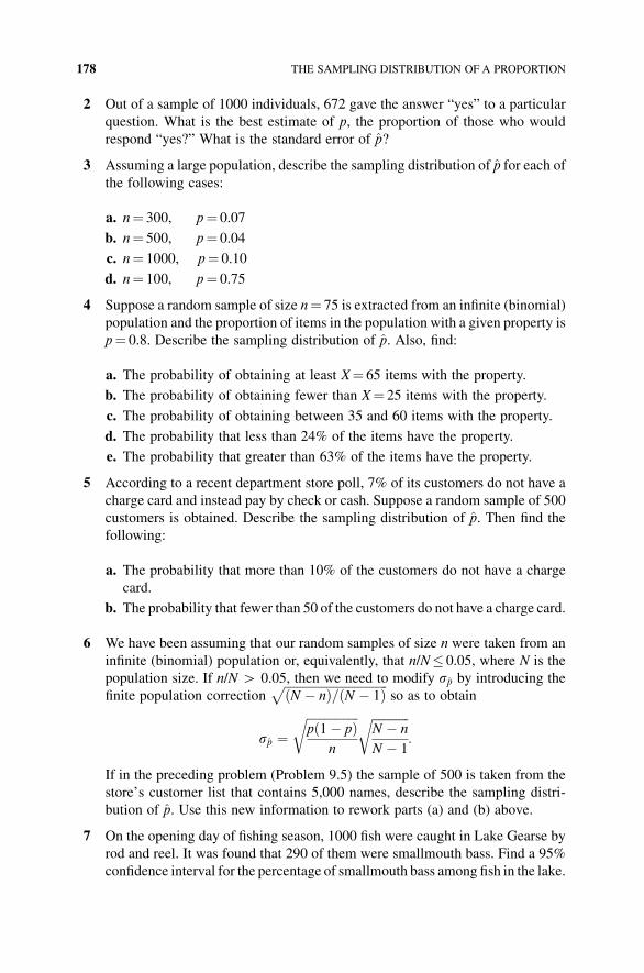
2 Out of a sample of 1000 individuals, 672 gave the answer “yes” to a particular
question. What is the best estimate of p, the proportion of those who would
respond “yes?” What is the standard error of p?
3 Assuming a large population, describe the sampling distribution of p for each of
the following cases:
a. n¼ 300, p¼ 0.07
b. n¼ 500, p¼ 0.04
c. n¼ 1000, p¼ 0.10
d. n¼ 100, p¼ 0.75
4 Suppose a random sample of size n¼ 75 is extracted from an infinite (binomial)
population and the proportion of items in the population with a given property is
p¼ 0.8. Describe the sampling distribution of p. Also, find:
a. The probability of obtaining at least X¼ 65 items with the property.
b. The probability of obtaining fewer than X¼ 25 items with the property.
c. The probability of obtaining between 35 and 60 items with the property.
d. The probability that less than 24% of the items have the property.
e. The probability that greater than 63% of the items have the property.
5 According to a recent department store poll, 7% of its customers do not have a
charge card and instead pay by check or cash. Suppose a random sample of 500
customers is obtained. Describe the sampling distribution of p. Then find the
following:
a. The probability that more than 10% of the customers do not have a charge
card.
b. The probability that fewer than 50 of the customers do not have a charge card.
6 We have been assuming that our random samples of size n were taken from an
infinite (binomial) population or, equivalently, that n/N� 0.05, where N is the
population size. If n/N H 0.05, then we need to modify sp by introducing the
finite population correctionffiffiffiffiffiffiffiffiffiffiffiffiffiffiffiffiffiffiffiffiffiffiffiffiffiffiffiffiffiffiffiffiffiffiN � nð Þ= N � 1ð Þp
so as to obtain
sp ¼ffiffiffiffiffiffiffiffiffiffiffiffiffiffiffiffiffip 1� pð Þ
n
r ffiffiffiffiffiffiffiffiffiffiffiffiN � n
N � 1
r:
If in the preceding problem (Problem 9.5) the sample of 500 is taken from the
store’s customer list that contains 5,000 names, describe the sampling distri-
bution of p. Use this new information to rework parts (a) and (b) above.
7 On the opening day of fishing season, 1000 fish were caught in Lake Gearse by
rod and reel. It was found that 290 of them were smallmouth bass. Find a 95%
confidence interval for the percentage of smallmouth bass among fish in the lake.
178 THE SAMPLING DISTRIBUTION OF A PROPORTION
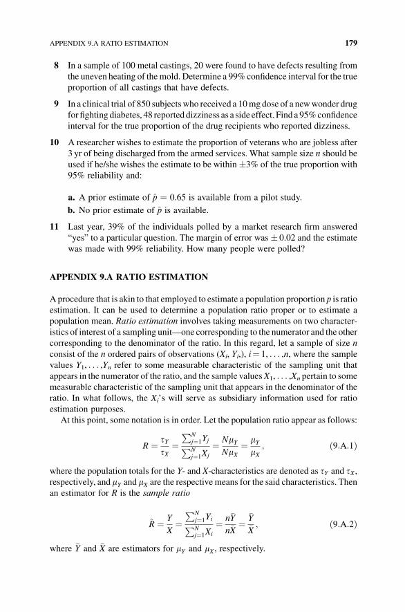
8 In a sample of 100 metal castings, 20 were found to have defects resulting from
the uneven heating of themold. Determine a 99% confidence interval for the true
proportion of all castings that have defects.
9 In a clinical trial of 850 subjects who received a 10mgdose of a newwonder drug
for fighting diabetes, 48 reported dizziness as a side effect. Find a 95%confidence
interval for the true proportion of the drug recipients who reported dizziness.
10 A researcher wishes to estimate the proportion of veterans who are jobless after
3 yr of being discharged from the armed services. What sample size n should be
used if he/she wishes the estimate to be within �3% of the true proportion with
95% reliability and:
a. A prior estimate of p ¼ 0.65 is available from a pilot study.
b. No prior estimate of p is available.
11 Last year, 39% of the individuals polled by a market research firm answered
“yes” to a particular question. The margin of error was � 0.02 and the estimate
was made with 99% reliability. How many people were polled?
APPENDIX 9.A RATIO ESTIMATION
Aprocedure that is akin to that employed to estimate a population proportion p is ratio
estimation. It can be used to determine a population ratio proper or to estimate a
population mean. Ratio estimation involves taking measurements on two character-
istics of interest of a sampling unit—one corresponding to the numerator and the other
corresponding to the denominator of the ratio. In this regard, let a sample of size n
consist of the n ordered pairs of observations (Xi, Yi,), i¼ 1, . . . ,n, where the sample
values Y1, . . . ,Yn refer to some measurable characteristic of the sampling unit that
appears in the numerator of the ratio, and the sample valuesX1, . . . ,Xn pertain to some
measurable characteristic of the sampling unit that appears in the denominator of the
ratio. In what follows, the Xi’s will serve as subsidiary information used for ratio
estimation purposes.
At this point, some notation is in order. Let the population ratio appear as follows:
R ¼ tYtX
¼PN
j¼1YjPNj¼1Xj
¼ NmYNmX
¼ mYmX
; ð9:A:1Þ
where the population totals for the Y- and X-characteristics are denoted as tY and tX ,respectively, and mY and mX are the respectivemeans for the said characteristics. Then
an estimator for R is the sample ratio
R ¼ Y
X¼
PNj¼1YiPNj¼1Xi
¼ n�Y
n�X¼
�Y�X; ð9:A:2Þ
where �Y and �X are estimators for mY and mX , respectively.
APPENDIX 9.A RATIO ESTIMATION 179
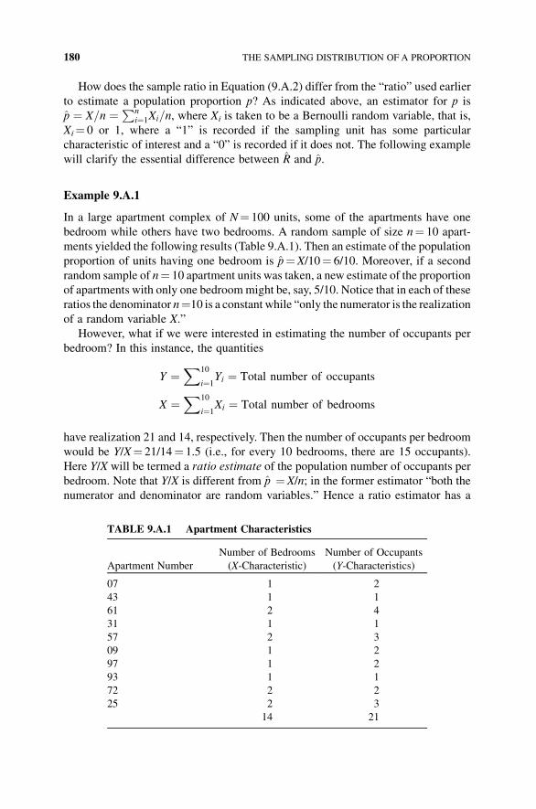
How does the sample ratio in Equation (9.A.2) differ from the “ratio” used earlier
to estimate a population proportion p? As indicated above, an estimator for p is
p ¼ X=n ¼ Pni¼1Xi=n, where Xi is taken to be a Bernoulli random variable, that is,
Xi¼ 0 or 1, where a “1” is recorded if the sampling unit has some particular
characteristic of interest and a “0” is recorded if it does not. The following example
will clarify the essential difference between R and p.
Example 9.A.1
In a large apartment complex of N¼ 100 units, some of the apartments have one
bedroom while others have two bedrooms. A random sample of size n¼ 10 apart-
ments yielded the following results (Table 9.A.1). Then an estimate of the population
proportion of units having one bedroom is p¼X/10¼ 6/10. Moreover, if a second
random sample of n¼ 10 apartment units was taken, a new estimate of the proportion
of apartments with only one bedroommight be, say, 5/10. Notice that in each of these
ratios the denominator n¼10 is a constant while “only the numerator is the realization
of a random variable X.”
However, what if we were interested in estimating the number of occupants per
bedroom? In this instance, the quantities
Y ¼X10
i¼1Yi ¼ Total number of occupants
X ¼X10
i¼1Xi ¼ Total number of bedrooms
have realization 21 and 14, respectively. Then the number of occupants per bedroom
would be Y/X¼ 21/14¼ 1.5 (i.e., for every 10 bedrooms, there are 15 occupants).
Here Y/X will be termed a ratio estimate of the population number of occupants per
bedroom. Note that Y/X is different from p ¼X/n; in the former estimator “both the
numerator and denominator are random variables.” Hence a ratio estimator has a
TABLE 9.A.1 Apartment Characteristics
Apartment Number
Number of Bedrooms
(X-Characteristic)
Number of Occupants
(Y-Characteristics)
07 1 2
43 1 1
61 2 4
31 1 1
57 2 3
09 1 2
97 1 2
93 1 1
72 2 2
25 2 3
14 21
180 THE SAMPLING DISTRIBUTION OF A PROPORTION
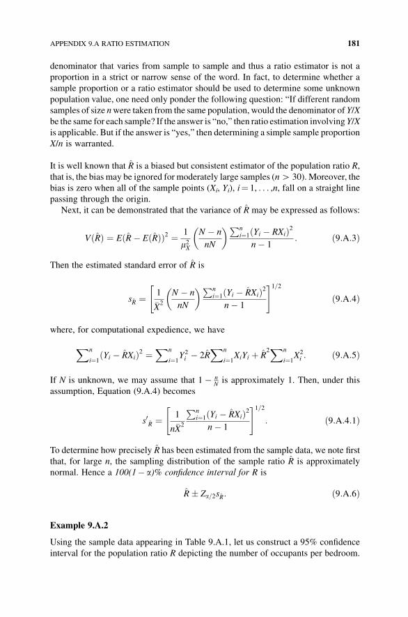
denominator that varies from sample to sample and thus a ratio estimator is not a
proportion in a strict or narrow sense of the word. In fact, to determine whether a
sample proportion or a ratio estimator should be used to determine some unknown
population value, one need only ponder the following question: “If different random
samples of size nwere taken from the same population, would the denominator of Y/X
be the same for each sample? If the answer is “no,” then ratio estimation involvingY/X
is applicable. But if the answer is “yes,” then determining a simple sample proportion
X/n is warranted.
It is well known that R is a biased but consistent estimator of the population ratio R,
that is, the bias may be ignored for moderately large samples (nH 30). Moreover, the
bias is zero when all of the sample points (Xi, Yi), i¼ 1, . . . ,n, fall on a straight line
passing through the origin.
Next, it can be demonstrated that the variance of R may be expressed as follows:
VðRÞ ¼ EðR� EðRÞÞ2 ¼ 1
m2X
N � n
nN
� �Pni¼1ðYi � RXiÞ2
n� 1: ð9:A:3Þ
Then the estimated standard error of R is
sR ¼ 1
�X2
N � n
nN
� �Pni¼1ðYi � RXiÞ2
n� 1
" #1=2
ð9:A:4Þ
where, for computational expedience, we have
Xn
i¼1ðYi � RXiÞ2 ¼
Xn
i¼1Y2i � 2R
Xn
i¼1XiYi þ R
2Xn
i¼1X2i : ð9:A:5Þ
If N is unknown, we may assume that 1� nNis approximately 1. Then, under this
assumption, Equation (9.A.4) becomes
s0R ¼ 1
n�X2
Pni¼1ðYi � RXiÞ2
n� 1
" #1=2
: ð9:A:4:1Þ
To determine how precisely R has been estimated from the sample data, we note first
that, for large n, the sampling distribution of the sample ratio R is approximately
normal. Hence a 100(1� a)% confidence interval for R is
R� Za=2sR: ð9:A:6Þ
Example 9.A.2
Using the sample data appearing in Table 9.A.1, let us construct a 95% confidence
interval for the population ratio R depicting the number of occupants per bedroom.
APPENDIX 9.A RATIO ESTIMATION 181
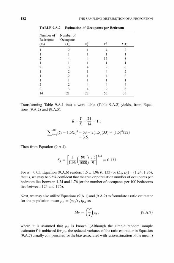
Transforming Table 9.A.1 into a work table (Table 9.A.2) yields, from Equa-
tions (9.A.2) and (9.A.5),
R ¼ Y
X¼ 21
14¼ 1:5
X10
i¼1ðYi � 1:5XiÞ2¼ 53� 2ð1:5Þð33Þ þ ð1:5Þ2ð22Þ
¼ 3:5:
Then from Equation (9.A.4),
SR ¼ 1
1:96
90
1000
� �3:5
9
� 1=2¼ 0:133:
For a¼ 0.05, Equation (9.A.6) renders 1.5� 1.96 (0.133) or (L1, L2)¼ (1.24, 1.76),
that is, we may be 95% confident that the true or population number of occupants per
bedroom lies between 1.24 and 1.76 (or the number of occupants per 100 bedrooms
lies between 124 and 176).
Next, wemay also utilize Equations (9.A.1) and (9.A.2) to formulate a ratio estimator
for the population mean mY ¼ ðtX=tYÞmX as
MY ¼�Y�X
� �mX; ð9:A:7Þ
where it is assumed that mX is known. (Although the simple random sample
estimator�Y is unbiased for mY, the reduced variance of the ratio estimator in Equation
(9.A.7) usually compensates for the bias associatedwith ratio estimation of themean.)
TABLE 9.A.2 Estimation of Occupants per Bedroom
Number of
Bedrooms
(Xi)
Number of
Occupants
(Yi) X2i Y2
i XiYi
1 2 1 4 2
1 1 1 1 1
2 4 4 16 8
1 1 1 1 1
2 3 4 9 6
1 2 1 4 2
1 2 1 4 2
1 1 1 1 1
2 2 4 4 4
2 3 4 9 6
14 21 22 53 33
182 THE SAMPLING DISTRIBUTION OF A PROPORTION
Moreover, the variance of MY is
VðMYÞ ¼ m2XVðRÞ ¼N � n
nN
� �Pni¼1ðYi � RXiÞ2
n� 1ð9:A:8Þ
and thus the estimated standard error of MY is
sMy¼ N � n
nN
� �Pni¼1ðYi � RXiÞ2
n� 1
" #1=2
: ð9:A:9Þ
And if we again assume a large sample n, then a 100(1� a)% confidence interval
for mY is given by
MY � Za=2sMY :
In sum, a ratio estimator is typically selected when:
a. The denominator in R is not n but is actually a random variable.
b. There is a strong association between a Y-characteristic and some supple-
mental or subsidiary X-characteristic in the population.
APPENDIX 9.A RATIO ESTIMATION 183
10TESTING STATISTICAL HYPOTHESES
The predominant operational theme addressed in this book is that of statistical
inference–drawing conclusions about a populationvia random sampling coupledwith
the use of probability theory to assess the reliability of those conclusions. There are
two sides to the “inferential coin,” so to speak. These are estimation and testing. As
indicated in Chapters 8 and 9, a confidence interval is used to estimate an unknown
parameter using sample data. As we shall now see, a hypothesis test (or significance
test) is carried out to determine how strong the sample evidence is regarding some
claim or assertion about a parameter.
We previously found that confidence interval estimation was based upon the
application of the sampling distribution of a statistic and its attendant probability
reckoning. The same is true of hypothesis testing. That is, hypothesis testing also
utilizes the concept of probability, obtained from the sampling distribution of a
statistic, to determinewhat would happen if we applied our test proceduremany times
in succession in the long run. It is the notion of probability that enables us to specify, in
a quantitative fashion, how credible our test results are.
10.1 WHAT IS A STATISTICAL HYPOTHESIS?
In general, a hypothesis is essentially an unproved theory or assertion; it is
tentatively accepted as an explanation of certain facts or observations. A statistical
hypothesis is a testable hypothesis—it specifies a value for some parameter (call it y)
Statistical Inference: A Short Course, First Edition. Michael J. Panik.� 2012 John Wiley & Sons, Inc. Published 2012 by John Wiley & Sons, Inc.
184
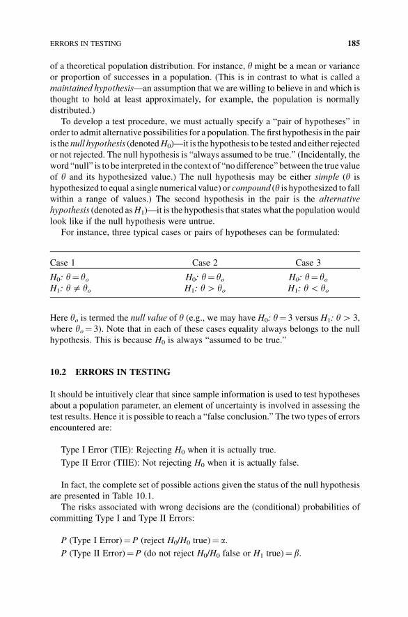
of a theoretical population distribution. For instance, y might be a mean or variance
or proportion of successes in a population. (This is in contrast to what is called a
maintained hypothesis—an assumption that we are willing to believe in and which is
thought to hold at least approximately, for example, the population is normally
distributed.)
To develop a test procedure, we must actually specify a “pair of hypotheses” in
order to admit alternative possibilities for a population. The first hypothesis in the pair
is the null hypothesis (denotedH0)—it is the hypothesis to be tested and either rejected
or not rejected. The null hypothesis is “always assumed to be true.” (Incidentally, the
word “null” is to be interpreted in the context of “no difference” between the truevalue
of y and its hypothesized value.) The null hypothesis may be either simple (y is
hypothesized to equal a single numerical value) or compound (y is hypothesized to fallwithin a range of values.) The second hypothesis in the pair is the alternative
hypothesis (denoted asH1)—it is the hypothesis that states what the population would
look like if the null hypothesis were untrue.
For instance, three typical cases or pairs of hypotheses can be formulated:
Case 1 Case 2 Case 3
H0: y¼ yo H0: y¼ yo H0: y¼ yoH1: y$ yo H1: yH yo H1: yG yo
Here yo is termed the null value of y (e.g., we may have H0: y¼ 3 versus H1: yH 3,
where yo¼ 3). Note that in each of these cases equality always belongs to the null
hypothesis. This is because H0 is always “assumed to be true.”
10.2 ERRORS IN TESTING
It should be intuitively clear that since sample information is used to test hypotheses
about a population parameter, an element of uncertainty is involved in assessing the
test results. Hence it is possible to reach a “false conclusion.” The two types of errors
encountered are:
Type I Error (TIE): Rejecting H0 when it is actually true.
Type II Error (TIIE): Not rejecting H0 when it is actually false.
In fact, the complete set of possible actions given the status of the null hypothesis
are presented in Table 10.1.
The risks associated with wrong decisions are the (conditional) probabilities of
committing Type I and Type II Errors:
P (Type I Error)¼P (reject H0/H0 true)¼ a.P (Type II Error)¼P (do not reject H0/H0 false or H1 true)¼ b.
ERRORS IN TESTING 185
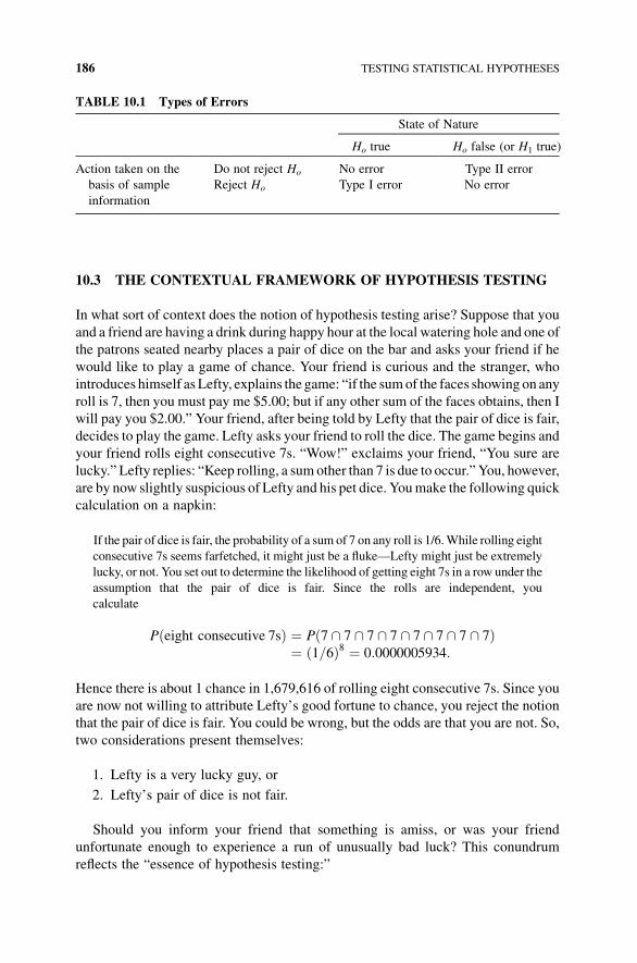
10.3 THE CONTEXTUAL FRAMEWORK OF HYPOTHESIS TESTING
In what sort of context does the notion of hypothesis testing arise? Suppose that you
and a friend are having a drink during happy hour at the local watering hole and one of
the patrons seated nearby places a pair of dice on the bar and asks your friend if he
would like to play a game of chance. Your friend is curious and the stranger, who
introduces himself as Lefty, explains the game: “if the sumof the faces showing on any
roll is 7, then you must pay me $5.00; but if any other sum of the faces obtains, then I
will pay you $2.00.” Your friend, after being told by Lefty that the pair of dice is fair,
decides to play the game. Lefty asks your friend to roll the dice. The game begins and
your friend rolls eight consecutive 7s. “Wow!” exclaims your friend, “You sure are
lucky.” Lefty replies: “Keep rolling, a sumother than 7 is due to occur.”You, however,
are by now slightly suspicious of Lefty and his pet dice. Youmake the following quick
calculation on a napkin:
If the pair of dice is fair, the probability of a sum of 7 on any roll is 1/6.While rolling eight
consecutive 7s seems farfetched, it might just be a fluke—Lefty might just be extremely
lucky, or not. You set out to determine the likelihood of getting eight 7s in a row under the
assumption that the pair of dice is fair. Since the rolls are independent, you
calculate
P eight consecutive 7sð Þ ¼ P 7 \ 7 \ 7 \ 7 \ 7 \ 7 \ 7 \ 7ð Þ¼ 1=6ð Þ8 ¼ 0:0000005934:
Hence there is about 1 chance in 1,679,616 of rolling eight consecutive 7s. Since you
are now not willing to attribute Lefty’s good fortune to chance, you reject the notion
that the pair of dice is fair. You could be wrong, but the odds are that you are not. So,
two considerations present themselves:
1. Lefty is a very lucky guy, or
2. Lefty’s pair of dice is not fair.
Should you inform your friend that something is amiss, or was your friend
unfortunate enough to experience a run of unusually bad luck? This conundrum
reflects the “essence of hypothesis testing:”
TABLE 10.1 Types of Errors
State of Nature
Ho true Ho false (or H1 true)
Action taken on the
basis of sample
information
Do not reject Ho No error Type II error
Reject Ho Type I error No error
186 TESTING STATISTICAL HYPOTHESES
(i) Youmake an assumption about the state of nature. (The probability of rolling
a 7 with a fair pair of dice is 1/6 or H0: P(7)¼ 1/6. Your suspicion regarding
Lefty’s pair of dice is that P(7)H 1/6 or H1: P(7)H 1/6.)
(ii) You gather sample evidence. (You feel that eight rolls of the pair of dice is
adequate for the experiment at hand.)
(iii) You determine if the sample evidence (under the assumption about the state
of nature) contradicts H0. You feel that it does because the probability of
getting eight 7s in a row “if H0 were true” is “too small” to be attributed
exclusively to sampling variation alone. Hence it is highly unlikely thatH0 is
true. Given the above probability result, a, the probability of a TIE, would beminiscule.
Other instances of formulating null and alternative hypotheses along with their
associated Type I and Type II Errors, are:
1. The manufacturer of a particular type of 6 v battery claims that it will last an
average of 400 hr under normal conditions in a particular model of camp
lantern. A Boy Scout troop leader wants to determine if the mean life of this
battery is overstated by the manufacturer. Here,
H0 : m ¼ mo ¼ 400
H1 : mG400:
TIE: Occurs if H0 is rejected when, in fact, H0 is true. A TIE is made if the
sample evidence leads the troop leader to believe that m is less than 400 hr
when, in actuality, m is not less than 400.
TIIE: Occurs ifH0 is not rejected when, in fact,H1 is true. ATIIE is made if the
sample evidence prompts the troop leader to not reject H0 when, in reality,
mG 400 hr.
2. ACE Packing and Transit Co. boasts of only a 1.5% breakage rate on items
shipped overnight. A dealer in glass art feels that this rate might be much too
low. Here,
H0 : p ¼ po ¼ 0:015H1 : pH0:015:
TIE:Occurs ifH0 is rejectedwhen it is actually true.ATIE ismadewhen sample
evidence prompts the dealer to believe pH 0.015 when, in fact, p does not
exceed 0.015.
TIIE: Occurs if H0 is not rejected when it is the case that H1 is true. A TIIE
ismade if the sample result leads the dealer to not rejectH0when, in actuality,
pH 0.015.
3. According to a spokesman from the outreach program of a local church group,
the mean value of clothing and other usable household items donated by
THE CONTEXTUAL FRAMEWORK OF HYPOTHESIS TESTING 187
parishioners over the last few years has been fairly stable at around $147.00 per
year. The pastorwants to determine if the level of givingwill be different for this
year. Now,
H0 : m ¼ mo ¼ $147:00
H1 : m$$147:00:
TIE: Occurs if H0 is rejected when, in reality, it is true. A TIE is made if the
sample data prompts the pastor to believe that m$ $147.00 when, in fact,
m¼ $147.00.
TIIE: Occurs ifH0 is not rejected whenH1 is true. ATIIE emerges if the sample
evidence leads the pastor to not rejectH0when it is the case thatm$ $147.00.
Some general and more commonplace environments involving hypothesis testing
now follows:
10.3.1 Types of Errors in a Legal Context
Suppose a felony trial is being conducted. Given our judicial system:
H0: The defendant is innocent (assumed true).
H1: The defendant is guilty.
The court seeks evidence for guilt. If the prosecutor cannot make a case, the jury
renders a verdict of “not guilty.” (Note that they do not declare the defendant
“innocent.” He/she may indeed be guilty, but the evidence against the defendant
was not compelling. This is why, in hypothesis testing, we say that we either “reject”
or “do not reject” H0. We don’t “accept” H0. The null hypothesis may actually be
untrue—it is just that the data could not discredit it.) What sorts of errors can occur?
TIE: Finding an innocent person guilty.
TIIE: Failing to convict a guilty person.
Type I Errors should be much less common than Type II Errors. The court will
tolerate a high probability of a Type II Error in order to diminish the probability of a
Type I Error. The legal system should avoid convicting an innocent person at all costs.
10.3.2 Types of Errors in a Medical Context
An individual is feeling poorly and goes to the local hospital emergency room. From
the viewpoint of the medical personnel:
H0: The individual is healthy (assumed true).
H1: The individual is unhealthy.
188 TESTING STATISTICAL HYPOTHESES
The doctors seek evidence that the person is unhealthy. Either the individual tests
positive for somemalady, or does not. Under this process, the person is never declared
“healthy;” the individualmay actually be unhealthy, but therewas insufficient clinical
evidence to uncover a medical problem. In this venue the types of errors are:
TIE: A healthy person tests positive (a false positive).
TIIE: An unhealthy person tests negative (a false negative).
Here Type II Errors should bemuch less common than Type I Errors. Type II Errors
can have dire consequences (treatment is withheld or delayed). Hence the medical
community will tolerate a high probability of a Type I Error in order to diminish
the probability of a Type II Error. Concluding that an unhealthy person is healthy
is anathema.
10.3.3 Types of Errors in a Processing or Control Context
A production manager is monitoring a temperature gauge for a plating process. The
temperature reading is supposed to vary only within a narrow range and the accuracy
of the gauge is critical if the plating material is to adhere to the host item. From the
viewpoint of the manager:
H0: The process is in control or working as designed.
H1: The process is not working as designed or is out of control.
The manager seeks evidence that the process is out of control. If it is, remedial
action must be taken. However, no action is warranted if the magnitude of any
temperature variation is deemed acceptable. In this environment, the errors that can be
made are:
TIE: Shutting down or adjusting a process that is in control.
TIIE: Letting a process that is out of control continue operating.
The probability of a Type II Error should be kept much lower than that of a Type I
Error since a production process delivering defective items could bemuchmore costly
to deal with (e.g., having to correct defects or scrap ruined items) than simply
attempting to modify a process that is currently operating correctly.
10.3.4 Types of Errors in a Sports Context
Conflicts over judgment calls occur all too frequently at sporting events. In making an
assessment of the efficacy of calls, we need to consider the possibility that:
H0: The referee’s or umpire’s call is correct.
H1: The referee’s or umpire’s call is erroneous.
THE CONTEXTUAL FRAMEWORK OF HYPOTHESIS TESTING 189
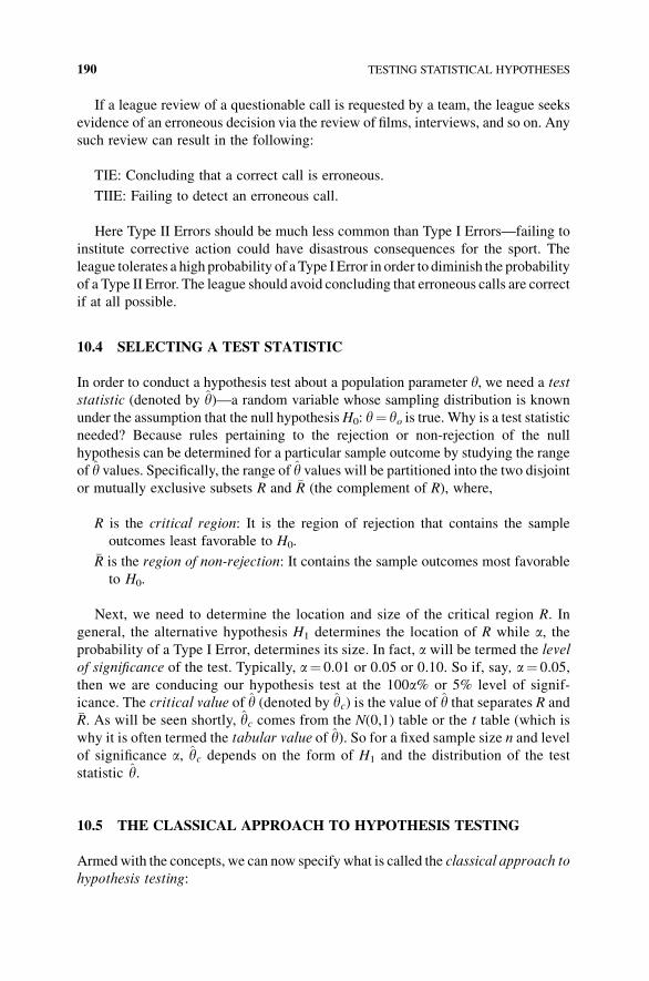
If a league review of a questionable call is requested by a team, the league seeks
evidence of an erroneous decision via the review of films, interviews, and so on. Any
such review can result in the following:
TIE: Concluding that a correct call is erroneous.
TIIE: Failing to detect an erroneous call.
Here Type II Errors should be much less common than Type I Errors—failing to
institute corrective action could have disastrous consequences for the sport. The
league tolerates a high probability of a Type I Error in order to diminish the probability
of a Type II Error. The league should avoid concluding that erroneous calls are correct
if at all possible.
10.4 SELECTING A TEST STATISTIC
In order to conduct a hypothesis test about a population parameter y, we need a test
statistic (denoted by y)—a random variable whose sampling distribution is known
under the assumption that the null hypothesisH0: y¼ yo is true. Why is a test statistic
needed? Because rules pertaining to the rejection or non-rejection of the null
hypothesis can be determined for a particular sample outcome by studying the range
of y values. Specifically, the range of y values will be partitioned into the two disjointor mutually exclusive subsets R and �R (the complement of R), where,
R is the critical region: It is the region of rejection that contains the sample
outcomes least favorable to H0.
�R is the region of non-rejection: It contains the sample outcomes most favorable
to H0.
Next, we need to determine the location and size of the critical region R. In
general, the alternative hypothesis H1 determines the location of R while a, theprobability of a Type I Error, determines its size. In fact, a will be termed the level
of significance of the test. Typically, a¼ 0.01 or 0.05 or 0.10. So if, say, a¼ 0.05,
then we are conducing our hypothesis test at the 100a% or 5% level of signif-
icance. The critical value of y (denoted by yc) is the value of y that separates R and�R. As will be seen shortly, yc comes from the N(0,1) table or the t table (which is
why it is often termed the tabular value of y). So for a fixed sample size n and level
of significance a, yc depends on the form of H1 and the distribution of the test
statistic y.
10.5 THE CLASSICAL APPROACH TO HYPOTHESIS TESTING
Armedwith the concepts, we can now specify what is called the classical approach to
hypothesis testing:
190 TESTING STATISTICAL HYPOTHESES
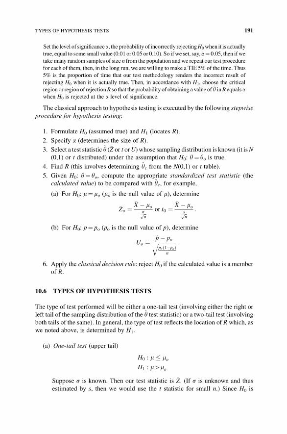
Set the level of significancea, the probability of incorrectly rejectingH0when it is actually
true, equal to some small value (0.01 or 0.05 or 0.10). So ifwe set, say, a¼ 0.05, then ifwe
takemany random samples of size n from the population andwe repeat our test procedure
for each of them, then, in the long run, we arewilling to make a TIE 5% of the time. Thus
5% is the proportion of time that our test methodology renders the incorrect result of
rejecting H0 when it is actually true. Then, in accordance with H1, choose the critical
region or region of rejectionR so that the probability of obtaining a value of y inR equals awhen H0 is rejected at the a level of significance.
The classical approach to hypothesis testing is executed by the following stepwise
procedure for hypothesis testing:
1. Formulate H0 (assumed true) and H1 (locates R).
2. Specify a (determines the size of R).
3. Select a test statistic y (�Z or t orU) whose sampling distribution is known (it isN
(0,1) or t distributed) under the assumption that H0: y¼ yo is true.4. Find R (this involves determining yc from the N(0,1) or t table).
5. Given H0: y¼ yo, compute the appropriate standardized test statistic (the
calculated value) to be compared with yc, for example,
(a) For H0: m¼ mo (mo is the null value of m), determine
�Zo ¼�X � mo
sffiffin
p or t0 ¼�X � mo
sffiffin
p :
(b) For H0: p¼ po (po is the null value of p), determine
Uo ¼ p� poffiffiffiffiffiffiffiffiffiffiffiffiffiffipoð1�poÞ
n
q :
6. Apply the classical decision rule: reject H0 if the calculated value is a member
of R.
10.6 TYPES OF HYPOTHESIS TESTS
The type of test performed will be either a one-tail test (involving either the right or
left tail of the sampling distribution of the y test statistic) or a two-tail test (involvingboth tails of the same). In general, the type of test reflects the location of R which, as
we noted above, is determined by H1.
(a) One-tail test (upper tail)
H0 : m � moH1 : mHmo
Suppose s is known. Then our test statistic is �Z. (If s is unknown and thus
estimated by s, then we would use the t statistic for small n.) Since H0 is
TYPES OF HYPOTHESIS TESTS 191
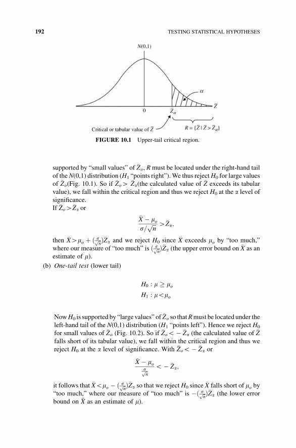
supported by “small values” of �Zo, Rmust be located under the right-hand tail
of theN(0,1) distribution (H1 “points right”).We thus rejectH0 for large values
of �Zo(Fig. 10.1). So if �ZoH �Za(the calculated value of �Z exceeds its tabular
value), we fall within the critical region and thus we reject H0 at the a level ofsignificance.
If �ZoH�Za or
�X � mos=
ffiffiffin
p H�Za;
then �XHmo þ ð sffiffin
p Þ�Za and we reject H0 since �X exceeds mo by “too much,”
where our measure of “too much” is ð sffiffin
p Þ�Za (the upper error bound on �X as an
estimate of m).(b) One-tail test (lower tail)
H0 : m � moH1 : mGmo
NowH0 is supported by “largevalues” of �Zo so thatRmust be located under the
left-hand tail of the N(0,1) distribution (H1 “points left”). Hence we reject H0
for small values of �Zo (Fig. 10.2). So if �ZoG� �Za (the calculated value of �Zfalls short of its tabular value), we fall within the critical region and thus we
reject H0 at the a level of significance. With �ZoG� �Za or
�X � mosffiffin
p G� �Za;
it follows that �XGmo � ð sffiffin
p Þ�Za so that we reject H0 since �X falls short of mo by“too much,” where our measure of “too much” is �ð sffiffi
np Þ�Za (the lower error
bound on �X as an estimate of m).
FIGURE 10.1 Upper-tail critical region.
192 TESTING STATISTICAL HYPOTHESES
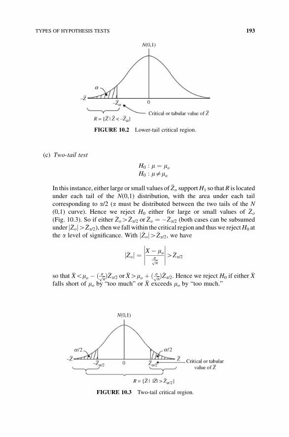
(c) Two-tail test
H0 : m ¼ moH0 : m$mo
In this instance, either large or small values of �Zo supportH1 so thatR is located
under each tail of the N(0,1) distribution, with the area under each tail
corresponding to a/2 (a must be distributed between the two tails of the N
(0,1) curve). Hence we reject H0 either for large or small values of �Zo
(Fig. 10.3). So if either �ZoH�Za/2 or �Zo ¼ ��Za/2 (both cases can be subsumed
under �Zoj jH�Za/2), thenwe fall within the critical region and thuswe rejectH0 at
the a level of significance. With �Zoj jH�Za/2, we have
�Zoj j ¼ X � mosffiffin
p
�����
�����H�Za/2
so that �XGmo � ð sffiffin
p Þ�Za/2 or �XHmo þ ð sffiffin
p Þ�Za/2. Hence we reject H0 if either �Xfalls short of mo by “too much” or �X exceeds mo by “too much.”
FIGURE 10.2 Lower-tail critical region.
FIGURE 10.3 Two-tail critical region.
TYPES OF HYPOTHESIS TESTS 193
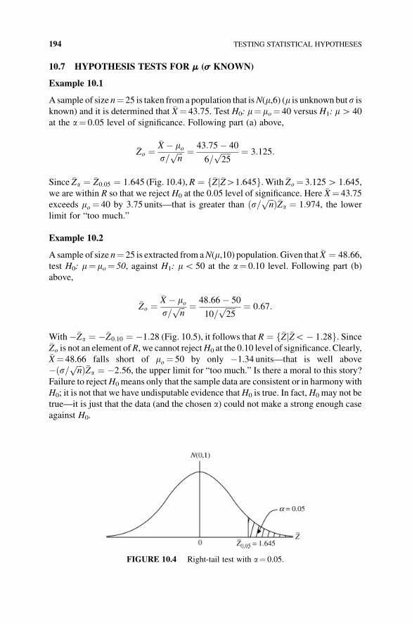
10.7 HYPOTHESIS TESTS FOR m (s KNOWN)
Example 10.1
Asample of size n¼ 25 is taken from a population that isN(m,6) (m is unknown buts isknown) and it is determined that �X¼ 43.75. Test H0: m¼ mo¼ 40 versus H1: mH 40
at the a¼ 0.05 level of significance. Following part (a) above,
�Zo ¼�X � mos=
ffiffiffin
p ¼ 43:75� 40
6=ffiffiffiffiffi25
p ¼ 3:125:
Since �Za ¼ �Z0:05 ¼ 1:645 (Fig. 10.4),R ¼ f�Zj�ZH1:645g. With �Zo ¼ 3.125H 1.645,
we are within R so that we reject H0 at the 0.05 level of significance. Here �X¼ 43.75
exceeds mo ¼ 40 by 3.75 units—that is greater than s=ffiffiffin
pð Þ�Za ¼ 1:974, the lower
limit for “too much.”
Example 10.2
Asample of size n¼ 25 is extracted from aN(m,10) population. Given that �X ¼ 48:66,test H0: m¼ mo¼ 50, against H1: mG 50 at the a¼ 0.10 level. Following part (b)
above,
�Zo ¼�X � mos=
ffiffiffin
p ¼ 48:66� 50
10=ffiffiffiffiffi25
p ¼ 0:67:
With��Za ¼ ��Z0:10 ¼ �1:28 (Fig. 10.5), it follows that R ¼ f�Zj�ZG� 1:28g. Since�Zo is not an element ofR, we cannot rejectH0 at the 0.10 level of significance. Clearly,�X¼ 48.66 falls short of mo ¼ 50 by only �1.34 units—that is well above
� s=ffiffiffin
pð Þ�Za ¼ �2:56, the upper limit for “too much.” Is there a moral to this story?
Failure to rejectH0 means only that the sample data are consistent or in harmonywith
H0; it is not that we have undisputable evidence thatH0 is true. In fact, H0 may not be
true—it is just that the data (and the chosen a) could not make a strong enough case
against H0.
FIGURE 10.4 Right-tail test with a¼ 0.05.
194 TESTING STATISTICAL HYPOTHESES
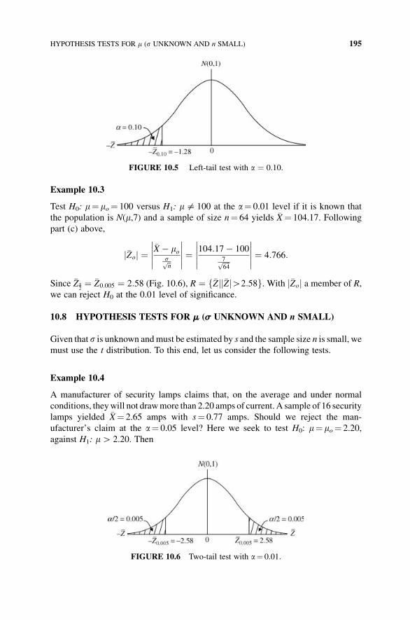
Example 10.3
Test H0: m¼ mo¼ 100 versus H1: m$ 100 at the a¼ 0.01 level if it is known that
the population is N(m,7) and a sample of size n¼ 64 yields �X¼ 104.17. Following
part (c) above,
�Zoj j ¼�X � mo
sffiffin
p
�����
����� ¼104:17� 100
7ffiffiffiffi64
p
�����
����� ¼ 4:766:
Since �Za2¼ �Z0:005 ¼ 2:58 (Fig. 10.6), R ¼ f�Zj �Zj jH2:58g. With �Zoj j a member of R,
we can reject H0 at the 0.01 level of significance.
10.8 HYPOTHESIS TESTS FOR m (s UNKNOWN AND n SMALL)
Given that s is unknown andmust be estimated by s and the sample size n is small, we
must use the t distribution. To this end, let us consider the following tests.
Example 10.4
A manufacturer of security lamps claims that, on the average and under normal
conditions, theywill not drawmore than 2.20 amps of current. A sample of 16 security
lamps yielded �X¼ 2.65 amps with s¼ 0.77 amps. Should we reject the man-
ufacturer’s claim at the a¼ 0.05 level? Here we seek to test H0: m¼ mo¼ 2.20,
against H1: mH 2.20. Then
FIGURE 10.5 Left-tail test with a ¼ 0.10.
FIGURE 10.6 Two-tail test with a¼ 0.01.
HYPOTHESIS TESTS FOR m (s UNKNOWN AND n SMALL) 195
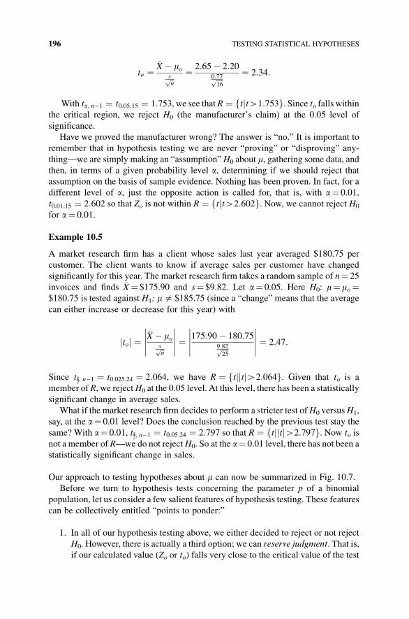
to ¼�X � mo
sffiffin
p ¼ 2:65� 2:200:77ffiffiffiffi16
p ¼ 2:34:
With ta; n�1 ¼ t0:05;15 ¼ 1:753, we see thatR ¼ ftjtH1:753g. Since to falls withinthe critical region, we reject H0 (the manufacturer’s claim) at the 0.05 level of
significance.
Have we proved the manufacturer wrong? The answer is “no.” It is important to
remember that in hypothesis testing we are never “proving” or “disproving” any-
thing—we are simply making an “assumption” H0 about m, gathering some data, and
then, in terms of a given probability level a, determining if we should reject that
assumption on the basis of sample evidence. Nothing has been proven. In fact, for a
different level of a, just the opposite action is called for, that is, with a¼ 0.01,
t0:01;15 ¼ 2:602 so that Zo is not within R ¼ ftjtH2:602g. Now, we cannot reject H0
for a¼ 0.01.
Example 10.5
A market research firm has a client whose sales last year averaged $180.75 per
customer. The client wants to know if average sales per customer have changed
significantly for this year. The market research firm takes a random sample of n¼ 25
invoices and finds �X¼ $175.90 and s¼ $9.82. Let a¼ 0.05. Here H0: m¼ mo¼$180.75 is tested against H1: m$ $185.75 (since a “change” means that the average
can either increase or decrease for this year) with
toj j ¼�X � mo
sffiffin
p
�����
����� ¼175:90� 180:75
9:82ffiffiffiffi25
p
�����
����� ¼ 2:47:
Since ta2; n�1 ¼ t0:025;24 ¼ 2:064, we have R ¼ ftj tj jH2:064g. Given that to is a
member of R, we rejectH0 at the 0.05 level. At this level, there has been a statistically
significant change in average sales.
What if the market research firm decides to perform a stricter test ofH0 versusH1,
say, at the a¼ 0.01 level? Does the conclusion reached by the previous test stay the
same? With a¼ 0.01, ta2; n�1 ¼ t0:05;24 ¼ 2:797 so that R ¼ ftj tj jH2:797g. Now to is
not a member of R—we do not rejectH0. So at the a¼ 0.01 level, there has not been a
statistically significant change in sales.
Our approach to testing hypotheses about m can now be summarized in Fig. 10.7.
Before we turn to hypothesis tests concerning the parameter p of a binomial
population, let us consider a few salient features of hypothesis testing. These features
can be collectively entitled “points to ponder:”
1. In all of our hypothesis testing above, we either decided to reject or not reject
H0. However, there is actually a third option; we can reserve judgment. That is,
if our calculated value (Zo or to) falls very close to the critical value of the test
196 TESTING STATISTICAL HYPOTHESES
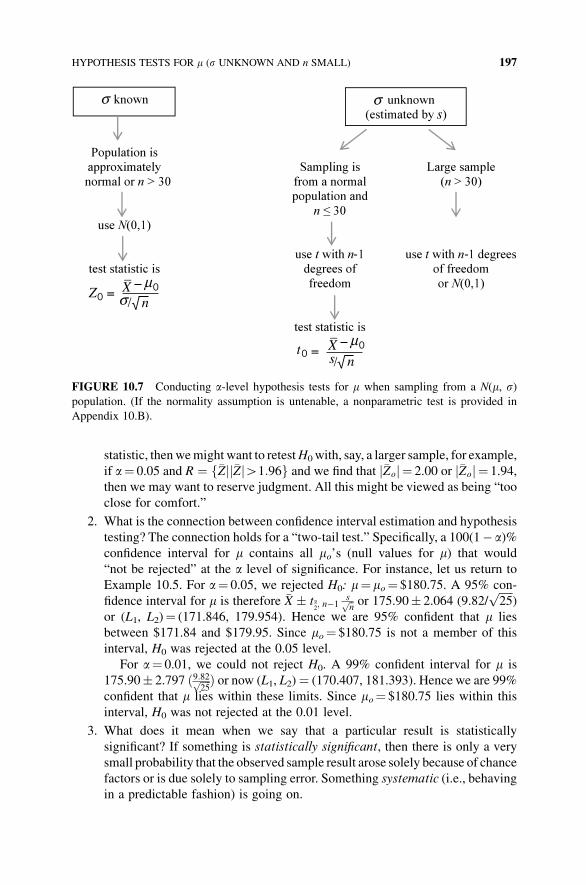
statistic, thenwemight want to retestH0 with, say, a larger sample, for example,
if a¼ 0.05 and R ¼ f�Zj �Zj jH1:96g and we find that �Zoj j ¼ 2.00 or �Zoj j ¼ 1.94,
then we may want to reserve judgment. All this might be viewed as being “too
close for comfort.”
2. What is the connection between confidence interval estimation and hypothesis
testing? The connection holds for a “two-tail test.” Specifically, a 100(1� a)%confidence interval for m contains all mo’s (null values for m) that would
“not be rejected” at the a level of significance. For instance, let us return to
Example 10.5. For a¼ 0.05, we rejected H0: m¼ mo¼ $180.75. A 95% con-
fidence interval for m is therefore �X � ta2; n�1
sffiffin
p or 175.90� 2.064 (9.82/ffiffiffiffiffi25
p)
or (L1, L2)¼ (171.846, 179.954). Hence we are 95% confident that m lies
between $171.84 and $179.95. Since mo¼ $180.75 is not a member of this
interval, H0 was rejected at the 0.05 level.
For a¼ 0.01, we could not reject H0. A 99% confident interval for m is
175.90� 2.797 ð9:82ffiffiffiffi25
p Þ or now (L1, L2)¼ (170.407, 181.393). Hence we are 99%
confident that m lies within these limits. Since mo¼ $180.75 lies within this
interval, H0 was not rejected at the 0.01 level.
3. What does it mean when we say that a particular result is statistically
significant? If something is statistically significant, then there is only a very
small probability that the observed sample result arose solely because of chance
factors or is due solely to sampling error. Something systematic (i.e., behaving
in a predictable fashion) is going on.
σ
σ/
/
μ
σs
Z
t
Xn
–
μX–
√
ns√
t
FIGURE 10.7 Conducting a-level hypothesis tests for m when sampling from a N(m, s)population. (If the normality assumption is untenable, a nonparametric test is provided in
Appendix 10.B).
HYPOTHESIS TESTS FOR m (s UNKNOWN AND n SMALL) 197
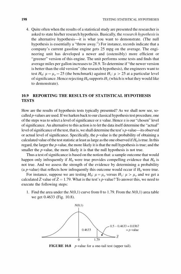
4. Quite often when the results of a statistical study are presented the researcher is
asked to state his/her research hypothesis. Basically, the research hypothesis is
the alternative hypothesis—it is what you want to demonstrate. (The null
hypothesis is essentially a “throw away.”) For instance, records indicate that a
company’s current gasoline engine gets 25 mpg on the average. The engi-
neering unit has developed a newer and (ostensibly) more efficient or
“greener” version of this engine. The unit performs some tests and finds that
average miles per gallon increases to 28.9. To determine if “the newer version
is better than the old version” (the research hypothesis), the engineers want to
test H0: m¼ mo¼ 25 (the benchmark) against H1: mH 25 at a particular level
of significance.Hence rejectingH0 supportsH1 (which iswhat theywould like
to demonstrate).
10.9 REPORTING THE RESULTS OF STATISTICAL HYPOTHESIS
TESTS
How are the results of hypothesis tests typically presented? As we shall now see, so-
calledp-values are used. Ifweharken back to our classical hypothesis test procedure, one
of the steps was to select a level of significance or a value. Hence a is our “chosen” levelof significance. An alternative to this action is to let the data itself determine the “actual”
level of significanceof the test, that is,we shall determine the test’sp-value—itsobserved
or actual level of significance. Specifically, the p-value is the probability of obtaining a
calculated value of the test statistic at least as large as theoneobserved ifH0 is true. In this
regard, the larger the p-value, themore likely it is that the null hypothesis is true; and the
smaller the p-value, the more likely it is that the null hypothesis is not true.
Thus a test of significance is based on the notion that: a sample outcome that would
happen only infrequently if H0 were true provides compelling evidence that H0 is
not true. And we assess the strength of the evidence by determining a probability
(a p-value) that reflects how infrequently this outcome would occur if H0 were true.
For instance, suppose we are testing H0: m¼ mo versus H1: mH mo and we get a
calculated �Z value of �Z¼ 1.79. What is the test’s p-value? To answer this, we need to
execute the following steps:
1. Find the area under the N(0,1) curve from 0 to 1.79. From the N(0,1) area table
we get 0.4633 (Fig. 10.8).
FIGURE 10.8 p-value for a one-tail test (upper tail).
198 TESTING STATISTICAL HYPOTHESES
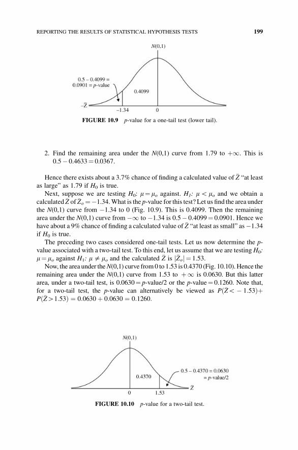
2. Find the remaining area under the N(0,1) curve from 1.79 to þ1. This is
0.5� 0.4633¼ 0.0367.
Hence there exists about a 3.7% chance of finding a calculated value of �Z “at least
as large” as 1.79 if H0 is true.
Next, suppose we are testing H0: m¼ mo against. H1: mG mo and we obtain a
calculated �Z of �Zo ¼�1.34.What is the p-value for this test? Let us find the area under
the N(0,1) curve from �1.34 to 0 (Fig. 10.9). This is 0.4099. Then the remaining
area under the N(0,1) curve from �1 to �1.34 is 0.5� 0.4099¼ 0.0901. Hence we
have about a 9% chance of finding a calculated value of �Z “at least as small” as�1.34
if H0 is true.
The preceding two cases considered one-tail tests. Let us now determine the p-
value associated with a two-tail test. To this end, let us assume that we are testingH0:
m¼ mo against H1: m$ mo and the calculated �Z is �Zoj j ¼ 1.53.
Now, the area under theN(0,1) curve from0 to 1.53 is 0.4370 (Fig. 10.10). Hence the
remaining area under the N(0,1) curve from 1.53 to þ1 is 0.0630. But this latter
area, under a two-tail test, is 0.0630¼ p-value/2 or the p-value¼ 0.1260. Note that,
for a two-tail test, the p-value can alternatively be viewed as Pð�ZG� 1:53ÞþPð�ZH1:53Þ ¼ 0:0630þ 0:0630 ¼ 0:1260:
FIGURE 10.9 p-value for a one-tail test (lower tail).
FIGURE 10.10 p-value for a two-tail test.
REPORTING THE RESULTS OF STATISTICAL HYPOTHESIS TESTS 199
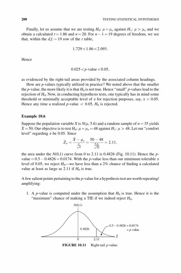
Finally, let us assume that we are testing H0: m¼ mo against H1: mH mo and we
obtain a calculated t¼ 1.86 and n¼ 20. For n� 1¼ 19 degrees of freedom, we see
that, within the d.f.¼ 19 row of the t table,
1:729G1:86G2:093:
Hence
0:025Gp-valueG0:05;
as evidenced by the right-tail areas provided by the associated column headings.
How are p-values typically utilized in practice? We noted above that the smaller
the p-value, the more likely it is thatH0 is not true. Hence “small” p-values lead to the
rejection of H0. Now, in conducting hypothesis tests, one typically has in mind some
threshold or minimally acceptable level of a for rejection purposes, say, a ¼ 0.05.
Hence any time a realized p-value G 0.05, H0 is rejected.
Example 10.6
Suppose the population variable X is N(m, 5.6) and a random sample of n¼ 35 yields�X¼ 50. Our objective is to testH0: m¼ mo¼ 48 againstH1: mH 48. Let our “comfort
level” regarding a be 0.05. Since
�Zo ¼�X � mo
sffiffin
p ¼ 50� 485:6ffiffiffiffi35
p ¼ 2:11;
the area under the N(0,1) curve from 0 to 2.11 is 0.4826 (Fig. 10.11). Hence the p-
value¼ 0.5� 0.4826¼ 0.0174. With the p-value less than our minimum tolerable alevel of 0.05, we reject H0—we have less than a 2% chance of finding a calculated
value at least as large as 2.11 if H0 is true.
A few salient points pertaining to the p-value for a hypothesis test areworth repeating/
amplifying:
1. A p-value is computed under the assumption that H0 is true. Hence it is the
“maximum” chance of making a TIE if we indeed reject H0.
FIGURE 10.11 Right-tail p-value.
200 TESTING STATISTICAL HYPOTHESES
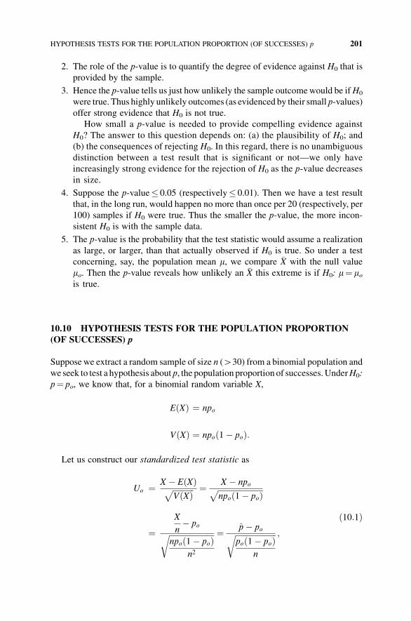
2. The role of the p-value is to quantify the degree of evidence against H0 that is
provided by the sample.
3. Hence the p-value tells us just how unlikely the sample outcomewould be ifH0
were true. Thus highly unlikely outcomes (as evidenced by their small p-values)
offer strong evidence that H0 is not true.
How small a p-value is needed to provide compelling evidence against
H0? The answer to this question depends on: (a) the plausibility of H0; and
(b) the consequences of rejecting H0. In this regard, there is no unambiguous
distinction between a test result that is significant or not—we only have
increasingly strong evidence for the rejection of H0 as the p-value decreases
in size.
4. Suppose the p-value� 0.05 (respectively� 0.01). Then we have a test result
that, in the long run, would happen no more than once per 20 (respectively, per
100) samples if H0 were true. Thus the smaller the p-value, the more incon-
sistent H0 is with the sample data.
5. The p-value is the probability that the test statistic would assume a realization
as large, or larger, than that actually observed if H0 is true. So under a test
concerning, say, the population mean m, we compare �X with the null value
mo. Then the p-value reveals how unlikely an �X this extreme is if H0: m¼ mois true.
10.10 HYPOTHESIS TESTS FOR THE POPULATION PROPORTION
(OF SUCCESSES) p
Supposewe extract a random sample of size n (H30) from a binomial population and
we seek to test a hypothesis about p, the population proportion of successes.UnderH0:
p¼ po, we know that, for a binomial random variable X,
E Xð Þ ¼ npo
V Xð Þ ¼ npo 1� poð Þ:
Let us construct our standardized test statistic as
Uo ¼ X � E Xð ÞffiffiffiffiffiffiffiffiffiffiffiV Xð Þp ¼ X � npoffiffiffiffiffiffiffiffiffiffiffiffiffiffiffiffiffiffiffiffiffiffiffi
npo 1� poð Þp
¼X
n� po
ffiffiffiffiffiffiffiffiffiffiffiffiffiffiffiffiffiffiffiffiffiffiffinpo 1� poð Þ
n2
r ¼ p� poffiffiffiffiffiffiffiffiffiffiffiffiffiffiffiffiffiffiffiffiffipo 1� poð Þ
n
r ;
ð10:1Þ
HYPOTHESIS TESTS FOR THE POPULATION PROPORTION (OF SUCCESSES) p 201
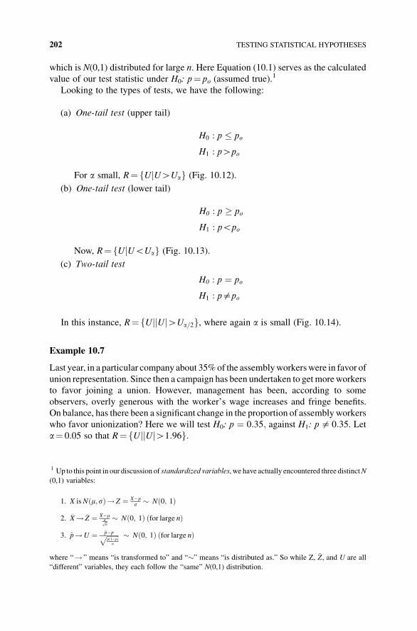
which is N(0,1) distributed for large n. Here Equation (10.1) serves as the calculated
value of our test statistic under H0: p¼ po (assumed true).1
Looking to the types of tests, we have the following:
(a) One-tail test (upper tail)
H0 : p � po
H1 : pHpo
For a small, R¼fUjUHUag (Fig. 10.12).
(b) One-tail test (lower tail)
H0 : p � po
H1 : pGpo
Now, R¼fUjUGUag (Fig. 10.13).
(c) Two-tail test
H0 : p ¼ po
H1 : p$po
In this instance, R¼fUjjUjHUa=2g, where again a is small (Fig. 10.14).
Example 10.7
Last year, in a particular company about 35%of the assemblyworkerswere in favor of
union representation. Since then a campaign has been undertaken to getmoreworkers
to favor joining a union. However, management has been, according to some
observers, overly generous with the worker’s wage increases and fringe benefits.
On balance, has there been a significant change in the proportion of assembly workers
who favor unionization? Here we will test H0: p ¼ 0:35; against H1: p$ 0:35. Leta¼ 0.05 so that R¼fUjjUjH1:96g:
1 Up to this point in our discussion of standardized variables, we have actually encountered three distinctN
(0,1) variables:
1. X isN m;sð Þ! Z ¼ X�ms � N 0; 1ð Þ
2. �X! �Z ¼ �X�msffiffin
p � N 0; 1ð Þ for large nð Þ
3. p!U ¼ p�pffiffiffiffiffiffiffiffip 1�pð Þ
n
p � N 0; 1ð Þ for large nð Þ
where “! ” means “is transformed to” and “�” means “is distributed as.” So while Z, �Z, and U are all
“different” variables, they each follow the “same” N(0,1) distribution.
202 TESTING STATISTICAL HYPOTHESES
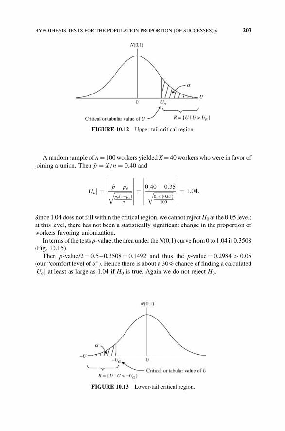
A random sample of n¼ 100workers yieldedX¼ 40workers whowere in favor of
joining a union. Then p ¼ X=n ¼ 0:40 and
Uoj j ¼ p� poffiffiffiffiffiffiffiffiffiffiffiffiffiffipo 1�poð Þ
n
q
�������
�������¼ 0:40� 0:35ffiffiffiffiffiffiffiffiffiffiffiffiffiffiffi
0:35 0:65ð Þ100
q
�������
�������¼ 1:04:
Since 1.04 does not fall within the critical region, we cannot rejectH0 at the 0.05 level;
at this level, there has not been a statistically significant change in the proportion of
workers favoring unionization.
In terms of the tests p-value, the area under theN(0,1) curve from0 to 1.04 is 0.3508
(Fig. 10.15).
Then p-value/2¼ 0.5�0.3508¼ 0.1492 and thus the p-value¼ 0.2984H 0.05
(our “comfort level of a”). Hence there is about a 30% chance of finding a calculated
Uoj j at least as large as 1.04 if H0 is true. Again we do not reject H0.
FIGURE 10.12 Upper-tail critical region.
FIGURE 10.13 Lower-tail critical region.
HYPOTHESIS TESTS FOR THE POPULATION PROPORTION (OF SUCCESSES) p 203
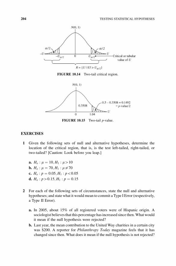
EXERCISES
1 Given the following sets of null and alternative hypotheses, determine the
location of the critical region, that is, is the test left-tailed, right-tailed, or
two-tailed? [Caution: Look before you leap.]
a. Ho : m ¼ 10;H1 : mH10
b. Ho : m ¼ 70;H1 : m$70
c. Ho : p ¼ 0:05;H1 : pG0:05
d. Ho : pH0:15;H1 : p ¼ 0:15
2 For each of the following sets of circumstances, state the null and alternative
hypotheses; and statewhat it wouldmean to commit a Type I Error (respectively,
a Type II Error).
a. In 2005, about 15% of all registered voters were of Hispanic origin. A
sociologist believes that this percentage has increased since then.Whatwould
it mean if the null hypothesis were rejected?
b. Last year, the mean contribution to the United Way charities in a certain city
was $200. A reporter for Philanthropy Today magazine feels that it has
changed since then. What does it mean if the null hypothesis is not rejected?
FIGURE 10.14 Two-tail critical region.
FIGURE 10.15 Two-tail p-value.
204 TESTING STATISTICAL HYPOTHESES
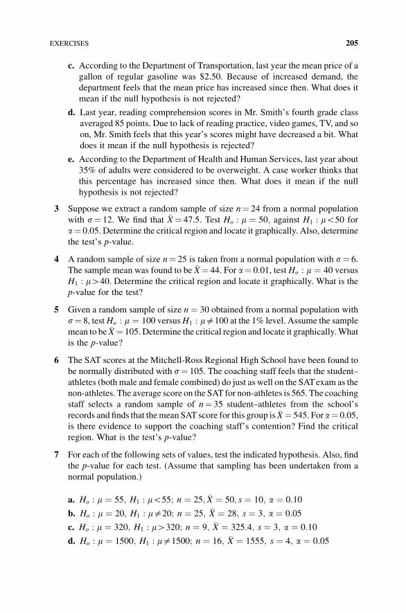
c. According to the Department of Transportation, last year the mean price of a
gallon of regular gasoline was $2.50. Because of increased demand, the
department feels that the mean price has increased since then. What does it
mean if the null hypothesis is not rejected?
d. Last year, reading comprehension scores in Mr. Smith’s fourth grade class
averaged 85 points. Due to lack of reading practice, video games, TV, and so
on, Mr. Smith feels that this year’s scores might have decreased a bit. What
does it mean if the null hypothesis is rejected?
e. According to the Department of Health and Human Services, last year about
35% of adults were considered to be overweight. A case worker thinks that
this percentage has increased since then. What does it mean if the null
hypothesis is not rejected?
3 Suppose we extract a random sample of size n¼ 24 from a normal population
with s¼ 12. We find that �X¼ 47.5. Test Ho : m ¼ 50; against H1 : mG50 for
a¼ 0.05. Determine the critical region and locate it graphically. Also, determine
the test’s p-value.
4 A random sample of size n¼ 25 is taken from a normal population with s¼ 6.
The sample mean was found to be �X¼ 44. For a¼ 0.01, testHo : m ¼ 40 versus
H1 : mH40. Determine the critical region and locate it graphically. What is the
p-value for the test?
5 Given a random sample of size n ¼ 30 obtained from a normal population with
s¼ 8, testHo : m ¼ 100 versusH1 : m$100 at the 1% level. Assume the sample
mean to be �X¼ 105. Determine the critical region and locate it graphically.What
is the p-value?
6 The SAT scores at the Mitchell-Ross Regional High School have been found to
be normally distributed with s¼ 105. The coaching staff feels that the student–
athletes (both male and female combined) do just as well on the SATexam as the
non-athletes. The average score on the SAT for non-athletes is 565. The coaching
staff selects a random sample of n¼ 35 student–athletes from the school’s
records and finds that themean SAT score for this group is �X¼ 545. For a¼ 0.05,
is there evidence to support the coaching staff’s contention? Find the critical
region. What is the test’s p-value?
7 For each of the following sets of values, test the indicated hypothesis. Also, find
the p-value for each test. (Assume that sampling has been undertaken from a
normal population.)
a. Ho : m ¼ 55; H1 : mG55; n ¼ 25; �X ¼ 50; s ¼ 10; a ¼ 0:10
b. Ho : m ¼ 20; H1 : m$20; n ¼ 25; �X ¼ 28; s ¼ 3; a ¼ 0:05
c. Ho : m ¼ 320; H1 : mH320; n ¼ 9; �X ¼ 325:4; s ¼ 3; a ¼ 0:10
d. Ho : m ¼ 1500; H1 : m$1500; n ¼ 16; �X ¼ 1555; s ¼ 4; a ¼ 0:05
EXERCISES 205
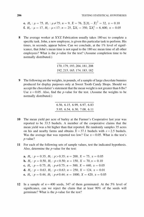
e. Ho : m ¼ 75; H1 : m$75; n ¼ 9; �X ¼ 76; S Xi � �Xð Þ2 ¼ 32; a ¼ 0:10
f. Ho : m ¼ 17; H1 : mG17; n ¼ 25; SXi ¼ 350; SX2i ¼ 6; 600; a ¼ 0:05
8 The average worker at XYZ Fabrication usually takes 180 sec to complete a
specific task. John, a new employee, is given this particular task to perform. His
times, in seconds, appear below. Can we conclude, at the 1% level of signif-
icance, that John’s mean time is not equal to the 180 sec mean time of all other
employees? What is the p-value for the test? (Assume completion time to be
normally distributed.)
170; 179; 193; 204; 181; 208
192; 215; 165; 174; 183; 182
9 The following are theweights, in pounds, of a sample of large chocolate bunnies
produced for display purposes only at Sweet Tooth Candy Shops. Should we
accept the chocolatier’s statement that the mean weight is not greater than 6 lbs?
Use a¼ 0.05. Also, find the p-value for the test. (Assume the weights to be
normally distributed.)
6:56; 6:15; 6:99; 6:97; 6:83
5:95; 6:54; 6:30; 7:08; 6:11
10 The mean yield per acre of barley at the Farmer’s Cooperative last year was
reported to be 33.5 bushels. A member of the cooperative claims that the
mean yield was a bit higher than that reported. He randomly samples 35 acres
on his and nearby farms and obtains �X¼ 37.1 bushels with s¼ 2.5 bushels.
Was the average that was reported too low? Use a¼ 0.05. What is the test’s
p-value?
11 For each of the following sets of sample values, test the indicated hypothesis.
Also, determine the p-value for the test:
a. Ho : p ¼ 0:35; H1 : pH0:35; n ¼ 200; X ¼ 75; a ¼ 0:05
b. Ho : p ¼ 0:50; H1 : pG0:50; n ¼ 150; X ¼ 70; a ¼ 0:10
c. Ho : p ¼ 0:75; H1 : p$0:75; n ¼ 500; X ¼ 440; a ¼ 0:05
d. Ho : p ¼ 0:63; H1 : pG0:63; n ¼ 250; X ¼ 124; a ¼ 0:01
e. Ho : p ¼ 0:44; H1 : p$0:44; n ¼ 1000; X ¼ 420; a ¼ 0:05
12 In a sample of n¼ 400 seeds, 347 of them germinated. At the 5% level of
significance, can we reject the claim that at least 90% of the seeds will
germinate? What is the p-value for the test?
206 TESTING STATISTICAL HYPOTHESES
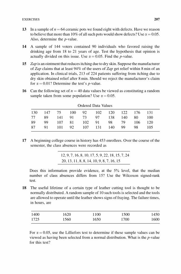
13 In a sample of n¼ 64 ceramic pots we found eight with defects. Have we reason
to believe that more than 10%of all such pots would show defects? Use a¼ 0.05.
Also, determine the p-value.
14 A sample of 144 voters contained 90 individuals who favored raising the
drinking age from 18 to 21 years of age. Test the hypothesis that opinion is
actually divided on this issue. Use a¼ 0.05. Find the p-value.
15 Zap is an ointment that reduces itching due to dry skin. Suppose themanufacturer
of Zap claims that at least 94% of the users of Zap get relief within 8min of an
application. In clinical trials, 213 of 224 patients suffering from itching due to
dry skin obtained relief after 8min. Should we reject the manufacturer’s claim
for a¼ 0.01? Determine the test’s p-value.
16 Can the following set of n ¼ 40 data values be viewed as constituting a random
sample taken from some population? Use a¼ 0.05.
Ordered Data Values
130 147 75 100 92 102 120 122 176 131
77 89 141 91 73 97 138 140 80 100
89 99 107 81 102 91 98 79 106 120
87 91 101 92 107 131 140 99 98 105
17 A beginning college course in history has 453 enrollees. Over the course of the
semester, the class absences were recorded as
12; 9; 7; 16; 8; 10; 17; 5; 9; 22; 18; 15; 7; 24
20; 13; 11; 8; 8; 14; 10; 9; 8; 7; 16; 15
Does this information provide evidence, at the 5% level, that the mediannumber of class absences differs from 15? Use the Wilcoxon signed-ranktest.
18 The useful lifetime of a certain type of leather cutting tool is thought to be
normally distributed. A random sample of 10 such tools is selected and the tools
are allowed to operate until the leather shows signs of fraying. The failure times,
in hours, are
1400 1620 1100 1500 1450
1725 1560 1650 1700 1600
For a¼ 0.05, use the Lilliefors test to determine if these sample values can be
viewed as having been selected from a normal distribution. What is the p-value
for this test?
EXERCISES 207
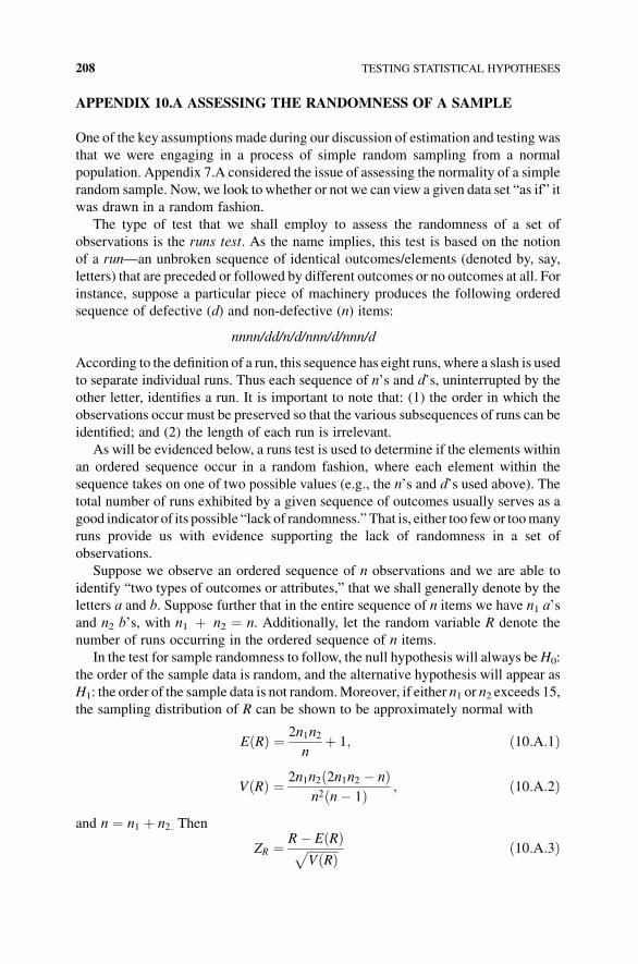
APPENDIX 10.A ASSESSING THE RANDOMNESS OF A SAMPLE
One of the key assumptions made during our discussion of estimation and testing was
that we were engaging in a process of simple random sampling from a normal
population. Appendix 7.A considered the issue of assessing the normality of a simple
random sample. Now, we look towhether or not we can view a given data set “as if” it
was drawn in a random fashion.
The type of test that we shall employ to assess the randomness of a set of
observations is the runs test. As the name implies, this test is based on the notion
of a run—an unbroken sequence of identical outcomes/elements (denoted by, say,
letters) that are preceded or followed by different outcomes or no outcomes at all. For
instance, suppose a particular piece of machinery produces the following ordered
sequence of defective (d) and non-defective (n) items:
nnnn/dd/n/d/nnn/d/nnn/d
According to the definition of a run, this sequence has eight runs, where a slash is used
to separate individual runs. Thus each sequence of n’s and d’s, uninterrupted by the
other letter, identifies a run. It is important to note that: (1) the order in which the
observations occur must be preserved so that the various subsequences of runs can be
identified; and (2) the length of each run is irrelevant.
As will be evidenced below, a runs test is used to determine if the elements within
an ordered sequence occur in a random fashion, where each element within the
sequence takes on one of two possible values (e.g., the n’s and d’s used above). The
total number of runs exhibited by a given sequence of outcomes usually serves as a
good indicator of its possible “lack of randomness.” That is, either too fewor toomany
runs provide us with evidence supporting the lack of randomness in a set of
observations.
Suppose we observe an ordered sequence of n observations and we are able to
identify “two types of outcomes or attributes,” that we shall generally denote by the
letters a and b. Suppose further that in the entire sequence of n items we have n1 a’s
and n2 b’s, with n1 þ n2 ¼ n. Additionally, let the random variable R denote the
number of runs occurring in the ordered sequence of n items.
In the test for sample randomness to follow, the null hypothesis will always beH0:
the order of the sample data is random, and the alternative hypothesis will appear as
H1: the order of the sample data is not random.Moreover, if either n1 or n2 exceeds 15,
the sampling distribution of R can be shown to be approximately normal with
E Rð Þ ¼ 2n1n2
nþ 1; ð10:A:1Þ
V Rð Þ ¼ 2n1n2 2n1n2 � nð Þn2 n� 1ð Þ ; ð10:A:2Þ
and n ¼ n1 þ n2. Then
ZR ¼ R� E Rð ÞffiffiffiffiffiffiffiffiffiffiV Rð Þp ð10:A:3Þ
208 TESTING STATISTICAL HYPOTHESES
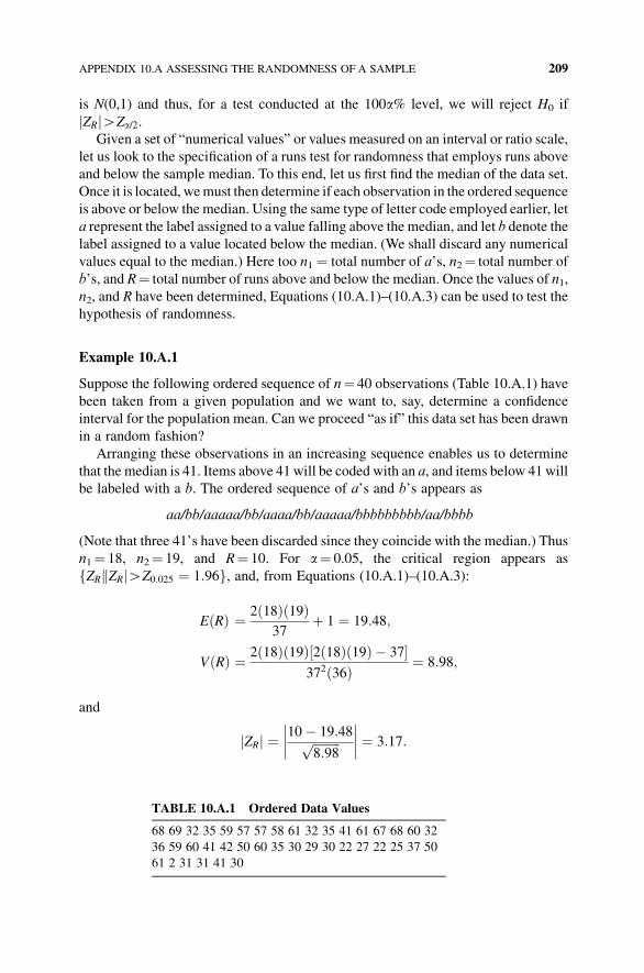
is N(0,1) and thus, for a test conducted at the 100a% level, we will reject H0 if
ZRj jHZa/2.
Given a set of “numerical values” or values measured on an interval or ratio scale,
let us look to the specification of a runs test for randomness that employs runs above
and below the sample median. To this end, let us first find the median of the data set.
Once it is located, wemust then determine if each observation in the ordered sequence
is above or below the median. Using the same type of letter code employed earlier, let
a represent the label assigned to a value falling above the median, and let b denote the
label assigned to a value located below the median. (We shall discard any numerical
values equal to the median.) Here too n1 ¼ total number of a’s, n2¼ total number of
b’s, and R¼ total number of runs above and below the median. Once the values of n1,
n2, and R have been determined, Equations (10.A.1)–(10.A.3) can be used to test the
hypothesis of randomness.
Example 10.A.1
Suppose the following ordered sequence of n¼ 40 observations (Table 10.A.1) have
been taken from a given population and we want to, say, determine a confidence
interval for the population mean. Can we proceed “as if” this data set has been drawn
in a random fashion?
Arranging these observations in an increasing sequence enables us to determine
that the median is 41. Items above 41 will be coded with an a, and items below 41 will
be labeled with a b. The ordered sequence of a’s and b’s appears as
aa/bb/aaaaa/bb/aaaa/bb/aaaaa/bbbbbbbbb/aa/bbbb
(Note that three 41’s have been discarded since they coincide with the median.) Thus
n1¼ 18, n2¼ 19, and R¼ 10. For a¼ 0.05, the critical region appears as
fZRkZRjHZ0:025 ¼ 1:96g, and, from Equations (10.A.1)–(10.A.3):
E Rð Þ ¼ 2 18ð Þ 19ð Þ37
þ 1 ¼ 19:48;
V Rð Þ ¼ 2 18ð Þ 19ð Þ 2 18ð Þ 19ð Þ � 37½ �372 36ð Þ ¼ 8:98;
and
ZRj j ¼ 10� 19:48ffiffiffiffiffiffiffiffiffi8:98
p����
���� ¼ 3:17:
TABLE 10.A.1 Ordered Data Values
68 69 32 35 59 57 57 58 61 32 35 41 61 67 68 60 32
36 59 60 41 42 50 60 35 30 29 30 22 27 22 25 37 50
61 2 31 31 41 30
APPENDIX 10.A ASSESSING THE RANDOMNESS OF A SAMPLE 209
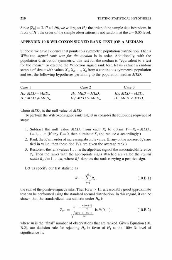
Since ZRj j ¼ 3:17H1:96;wewill rejectH0: the order of the sample data is random, in
favor ofH1: the order of the sample observations is not random, at the a¼ 0.05 level.
APPENDIX 10.B WILCOXON SIGNED RANK TEST (OF A MEDIAN)
Suppose we have evidence that points to a symmetric population distribution. Then a
Wilcoxon signed rank test for the median is in order. Additionally, with the
population distribution symmetric, this test for the median is “equivalent to a test
for the mean.” To execute the Wilcoxon signed rank test, let us extract a random
sample of size n with values X1, X2, . . ., Xn from a continuous symmetric population
and test the following hypotheses pertaining to the population median MED:
Case 1 Case 2 Case 3
H0: MED¼MEDo H0: MED¼MEDo H0: MED¼MEDo
H1: MED$MEDo H1: MEDHMEDo H1: MEDGMEDo
where MEDo is the null value of MED.
Toperform theWilcoxon signed rank test, let us consider the following sequence of
steps:
1. Subtract the null value MEDo from each Xi to obtain Yi¼Xi�MEDo,
i¼ 1,. . .,n. (If any Yi¼ 0, then eliminate Xi and reduce n accordingly.)
2. Rank theYi’s in order of increasing absolutevalue. (If any of the nonzeroYi’s are
tied in value, then these tied Yi’s are given the average rank.)
3. Restore to the rank values 1, . . ., n the algebraic sign of the associated differenceYi. Then the ranks with the appropriate signs attached are called the signed
ranks Ri, i¼ 1, . . .,n, where Rþi denotes the rank carrying a positive sign.
Let us specify our test statistic as
Wþ ¼Xn
i¼1
Rþi ; ð10:B:1Þ
the sum of the positive signed ranks. Then for nH 15, a reasonably good approximate
test can be performed using the standard normal distribution. In this regard, it can be
shown that the standardized test statistic under H0 is
Zwþ ¼ wþ � m mþ1ð Þ4ffiffiffiffiffiffiffiffiffiffiffiffiffiffiffiffiffiffiffiffiffiffiffiffi
m mþ1ð Þ 2mþ1ð Þ24
q is N 0; 1ð Þ; ð10:B:2Þ
where m is the “final” number of observations that are ranked. Given Equation (10.
B.2), our decision rule for rejecting H0 in favor of H1 at the 100a % level of
significance is:
210 TESTING STATISTICAL HYPOTHESES
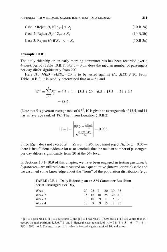
Case 1: RejectH0 if Zwþj jH Za2
10:B:3að ÞCase 2: Reject H0 if ZwþHZa 10:B:3bð ÞCase 3: Reject H0 if ZwþG� Za 10:B:3cð Þ
Example 10.B.1
The daily ridership on an early morning commuter bus has been recorded over a
4-week period (Table 10.B.1). For a¼ 0.05, does the median number of passengers
per day differ significantly from 20?
Here H0: MED¼MEDo¼ 20 is to be tested against H1: MED$ 20. From
Table 10.B.2, it is readily determined that m¼ 21 and
Wþ ¼X8
j¼1
Rþj ¼ 6:5þ 1þ 13:5þ 20þ 6:5þ 13:5 þ 21þ 6:5
¼ 88:5:
(Note that 5 is given an average rank of 6.52, 10 is given an average rank of 13.5, and 11
has an average rank of 18.) Then from Equation (10.B.2)
ZWþj j ¼ 88:5� 21 22ð Þ4ffiffiffiffiffiffiffiffiffiffiffiffiffiffiffiffi
21 22ð Þ 43ð Þ24
q
�������
�������¼ 0:938:
Since ZWþj j does not exceed Za2¼ Z0:025 ¼ 1:96; we cannot reject H0 for a¼ 0.05—
there is insufficient evidence for us to conclude that the median number of passengers
per day differs significantly from 20 at the 5% level.
In Sections 10.1–10.9 of this chapter, we have been engaged in testing parametric
hypotheses—we utilized data measured on a quantitative (interval or ratio) scale and
we assumed some knowledge about the “form” of the population distribution (e.g.,
TABLE 10.B.1 Daily Ridership on an AM Commuter Bus (Num-
ber of Passengers Per Day)
Week 1 20 25 21 20 30 35
Week 2 15 16 10 25 30 40
Week 3 10 10 9 11 15 20
Week 4 10 9 9 15 17 25
2 Yij j ¼ 1 gets rank 1, Yij j ¼ 3 gets rank 2, and Yij j ¼ 4 has rank 3. There are six Yij j ¼ 5 values that will
occupy the rank positions 4, 5, 6, 7, 8, and 9. Hence the average rank of Yij j ¼ 5 is (4 þ 5 þ 6 þ 7 þ 8 þ9)/6¼ 39/6¼ 6.5. The next largest Yij j value is 9—and it gets a rank of 10, and so on.
APPENDIX 10.B WILCOXON SIGNED RANK TEST (OF A MEDIAN) 211
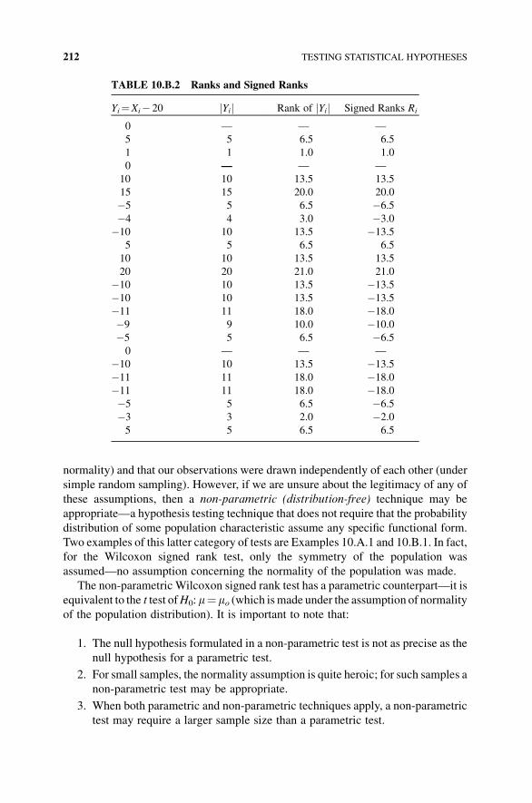
normality) and that our observations were drawn independently of each other (under
simple random sampling). However, if we are unsure about the legitimacy of any of
these assumptions, then a non-parametric (distribution-free) technique may be
appropriate—a hypothesis testing technique that does not require that the probability
distribution of some population characteristic assume any specific functional form.
Two examples of this latter category of tests are Examples 10.A.1 and 10.B.1. In fact,
for the Wilcoxon signed rank test, only the symmetry of the population was
assumed—no assumption concerning the normality of the population was made.
The non-parametric Wilcoxon signed rank test has a parametric counterpart—it is
equivalent to the t test ofH0:m¼ mo (which ismade under the assumption of normality
of the population distribution). It is important to note that:
1. The null hypothesis formulated in a non-parametric test is not as precise as the
null hypothesis for a parametric test.
2. For small samples, the normality assumption is quite heroic; for such samples a
non-parametric test may be appropriate.
3. When both parametric and non-parametric techniques apply, a non-parametric
test may require a larger sample size than a parametric test.
TABLE 10.B.2 Ranks and Signed Ranks
Yi¼Xi� 20 Yij j Rank of Yij j Signed Ranks Ri
0 — — —
5 5 6.5 6.5
1 1 1.0 1.0
0 — — —
10 10 13.5 13.5
15 15 20.0 20.0
�5 5 6.5 �6.5
�4 4 3.0 �3.0
�10 10 13.5 �13.5
5 5 6.5 6.5
10 10 13.5 13.5
20 20 21.0 21.0
�10 10 13.5 �13.5
�10 10 13.5 �13.5
�11 11 18.0 �18.0
�9 9 10.0 �10.0
�5 5 6.5 �6.5
0 — — —
�10 10 13.5 �13.5
�11 11 18.0 �18.0
�11 11 18.0 �18.0
�5 5 6.5 �6.5
�3 3 2.0 �2.0
5 5 6.5 6.5
212 TESTING STATISTICAL HYPOTHESES
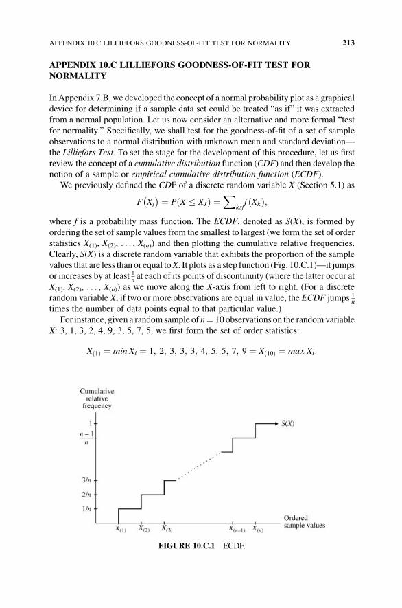
APPENDIX 10.C LILLIEFORS GOODNESS-OF-FIT TEST FOR
NORMALITY
InAppendix 7.B, we developed the concept of a normal probability plot as a graphical
device for determining if a sample data set could be treated “as if” it was extracted
from a normal population. Let us now consider an alternative and more formal “test
for normality.” Specifically, we shall test for the goodness-of-fit of a set of sample
observations to a normal distribution with unknown mean and standard deviation—
the Lilliefors Test. To set the stage for the development of this procedure, let us first
review the concept of a cumulative distribution function (CDF) and then develop the
notion of a sample or empirical cumulative distribution function (ECDF).
We previously defined the CDF of a discrete random variable X (Section 5.1) as
F Xj
� � ¼ P X � XJð Þ ¼X
ksjf Xkð Þ;
where f is a probability mass function. The ECDF, denoted as S(X), is formed by
ordering the set of sample values from the smallest to largest (we form the set of order
statistics X(1), X(2), . . . , X(n)) and then plotting the cumulative relative frequencies.
Clearly, S(X) is a discrete random variable that exhibits the proportion of the sample
values that are less than or equal toX. It plots as a step function (Fig. 10.C.1)—it jumps
or increases by at least 1nat each of its points of discontinuity (where the latter occur at
X(1), X(2), . . . , X(n)) as we move along the X-axis from left to right. (For a discrete
random variable X, if two or more observations are equal in value, the ECDF jumps 1n
times the number of data points equal to that particular value.)
For instance, given a random sample of n¼ 10 observations on the randomvariable
X: 3, 1, 3, 2, 4, 9, 3, 5, 7, 5, we first form the set of order statistics:
Xð1Þ ¼ min Xi ¼ 1; 2; 3; 3; 3; 4; 5; 5; 7; 9 ¼ Xð10Þ ¼ max Xi:
FIGURE 10.C.1 ECDF.
APPENDIX 10.C LILLIEFORS GOODNESS-OF-FIT TEST FOR NORMALITY 213
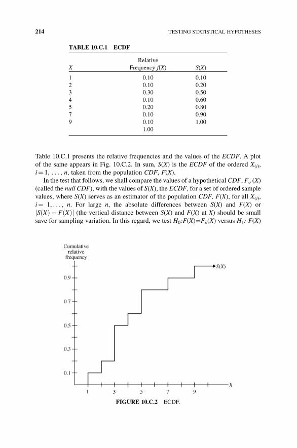
Table 10.C.1 presents the relative frequencies and the values of the ECDF. A plot
of the same appears in Fig. 10.C.2. In sum, S(X) is the ECDF of the ordered X(i),
i¼ 1, . . . , n, taken from the population CDF, F(X).
In the test that follows, we shall compare the values of a hypothetical CDF, Fo (X)
(called the null CDF), with the values of S(X), the ECDF, for a set of ordered sample
values, where S(X) serves as an estimator of the population CDF, F(X), for all X(i),
i¼ 1, . . . , n. For large n, the absolute differences between S(X) and F(X) or
S Xð Þ � F Xð Þj j (the vertical distance between S(X) and F(X) at X) should be small
save for sampling variation. In this regard, we test H0:F(X)¼Fo(X) versus H1: F(X)
TABLE 10.C.1 ECDF
X
Relative
Frequency f(X) S(X)
1 0.10 0.10
2 0.10 0.20
3 0.30 0.50
4 0.10 0.60
5 0.20 0.80
7 0.10 0.90
9 0.10 1.00
1.00
FIGURE 10.C.2 ECDF.
214 TESTING STATISTICAL HYPOTHESES
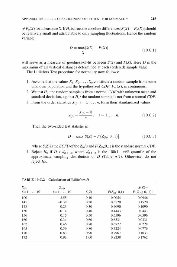
$Fo(X) for at least oneX. IfH0 is true, the absolute differences S Xð Þ � Fo Xð Þj j shouldbe relatively small and attributable to only sampling fluctuations. Hence the random
variable
D ¼ max S Xð Þ � F Xð Þj jX
ð10:C:1Þ
will serve as a measure of goodness-of-fit between S(X) and F(X). Here D is the
maximum of all vertical distances determined at each (ordered) sample value.
The Lilliefors Test procedure for normality now follows:
1. Assume that the values X1, X2, . . . , Xn constitute a random sample from some
unknown population and the hypothesized CDF, Fo (X), is continuous.
2. We testH0: the random sample is from a normal CDFwith unknown mean and
standard deviation, against H1: the random sample is not from a normal CDF.
3. From the order statistics X(i), i¼ 1, . . . , n, form their standardized values
Z ið Þ ¼X ið Þ � �X
s; i ¼ 1; . . . ; n: ð10:C:2Þ
Then the two-sided test statistic is
D ¼ max S Zð Þ � F Z ið Þ; 0; 1� ��� ��; ð10:C:3Þ
where S(Z) is theECFD of the Z(i)’s andF(Z(i);0,1) is the standard normalCDF.
4. Reject H0 if DH dn,1�a, where dn,1�a is the 100(1� a)% quantile of the
approximate sampling distribution of D (Table A.7). Otherwise, do not
reject H0.
TABLE 10.C.2 Calculation of Lilliefors D
X(i),
i¼ 1, . . . ,10Z(i),
i¼ 1, . . . ,10 S(Z) F(Z(i) ; 0,1)
S Zð Þ�jF Z Ið Þ; 0; 1� �j
100 �2.55 0.10 0.0054 0.0946
145 �0.38 0.20 0.3520 0.1520
148 �0.23 0.30 0.4090 0.1090
150 �0.14 0.40 0.4443 0.0443
156 0.15 0.50 0.5596 0.0596
160 0.34 0.60 0.6331 0.0331
162 0.46 0.70 0.6772 0.0228
165 0.59 0.80 0.7224 0.0776
170 0.83 0.90 0.7967 0.1033
172 0.93 1.00 0.8238 0.1762
APPENDIX 10.C LILLIEFORS GOODNESS-OF-FIT TEST FOR NORMALITY 215

Example 10.C.1
For 1� a¼ 0.95, determine if the following values of a random variable X can be
viewed as having been chosen from a normal distribution: 145, 150, 170, 100, 172,
160, 165, 156, 148, 162. For this data set, �X¼ 152.80 and s¼ 20.65. The ordered
sample values appear in Table 10.C.2 along with the Z(i)’s (e.g. for X(1)¼ 100,
Z(1)¼ (100� 152.80)/20.65¼�2,55). From Equation (10.C.3), D¼ 0.1762. Since
the critical region R ¼ fDjDH0:262g (see Table A.7), we cannot rejectH0 at the 5%
level of significance. Thus the normalCDF seems to be a reasonable representation of
the unknown population CDF.
216 TESTING STATISTICAL HYPOTHESES
11COMPARING TWO POPULATIONMEANS AND TWO POPULATIONPROPORTIONS
11.1 CONFIDENCE INTERVALS FOR THE DIFFERENCE
OF MEANS WHEN SAMPLING FROM TWO INDEPENDENT
NORMAL POPULATIONS
Let X1;X2; . . . ;XnXf g and Y1; Y2; . . . ; YnYf g be random samples taken from inde-
pendent normal distributions with means mX and mY and variances s2X and s2Y ,respectively. Our goal is to obtain a 100(1� a)% confidence interval for the difference
ofmeans mX � mY . To accomplish this task, wemust first examine the properties of the
sampling distribution of the difference between two sample means.
Suppose X and Y are independent random variables, where X is NðmX; sXÞ and Y is
NðmY ; sYÞ. For �X � �Y to serve as an estimator for mX � mY, we need to study the
properties of the distribution of �X � �Y given that we are sampling from two
independent normal populations. The following special cases present themselves.
11.1.1 Sampling from Two Independent Normal Populations with Equal
and Known Variances
We first assume that the population variances are equal and known or s2X ¼ s2Y¼ s2 is known. Then, from Chapter 7, �X is NðmX; s=
ffiffiffiffiffinX
p Þ and �Y is NðmY ; s=ffiffiffiffiffinY
p Þ.
Statistical Inference: A Short Course, First Edition. Michael J. Panik.� 2012 John Wiley & Sons, Inc. Published 2012 by John Wiley & Sons, Inc.
217
With �X and �Y independent normally distributed randomvariables, it can be shown that�X � �Y is normally distributedwithmeanmX � mY and variance ðs2X=nXÞ þ ðs2Y=nYÞ ¼s2 1
nXþ 1
nY
� �. Then with s2 known, the quantity
ZDm ¼ ðX � YÞ � ðmX � mYÞsffiffiffiffiffiffiffiffiffiffiffiffiffi1nXþ 1
nY
q is N ð0; 1Þ: ð11:1Þ
Hence a 100 (1� a)% confidence interval for mX � mY when s2X ¼ s2Y ¼ s2 is
known is
�X � �Yð Þ � Za=2s
ffiffiffiffiffiffiffiffiffiffiffiffiffiffiffiffi1
nXþ 1
nY
r: ð11:2Þ
11.1.2 Sampling from Two Independent Normal Populations with Unequal
but Known Variances
If the population variances are unequal but still assumed to be known, then the
quantity
Z 0Dm ¼ ð�X � �YÞ � mX � mYffiffiffiffiffiffiffiffiffiffiffiffiffiffi
s2X
nXþ s2
Y
nY
q is Nð0; 1Þ: ð11:3Þ
In this instance, a 100(1� a)% confidence interval for mX � mY when s2X and s2X
are known is
�X � �Yð Þ � Za=2
ffiffiffiffiffiffiffiffiffiffiffiffiffiffiffiffis2XnX
þ s2YnY
s
: ð11:4Þ
11.1.3 Sampling from Two Independent Normal Populations with Equal
but Unknown Variances
If the common variance s2 ¼s2X ¼ s2Y� �
is unknown, then we need to examine
the distribution of �X � �Y under sampling from two independent normal populations
with unknown but equal variances. Let the individual X and Y sample variances be
written as
s2X ¼
XnX
i¼1
Xi � �Xð Þ2
nX � 1and s2Y ¼
XnY
i¼1
Yi � �Yð Þ2
nY � 1
218 COMPARING TWO POPULATION MEANS AND TWO POPULATION PROPORTIONS
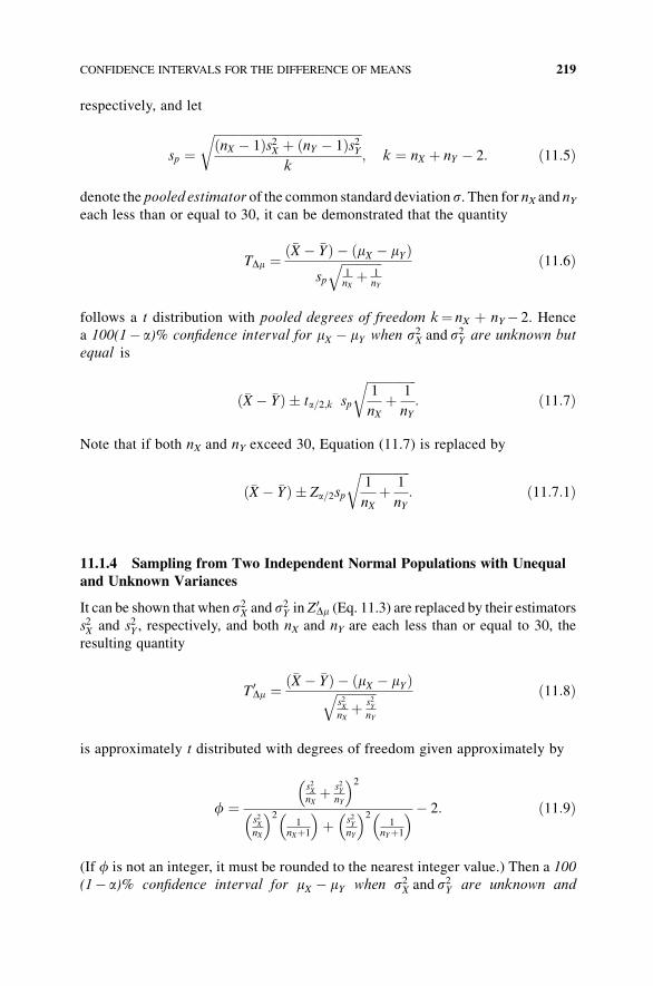
respectively, and let
sp ¼ffiffiffiffiffiffiffiffiffiffiffiffiffiffiffiffiffiffiffiffiffiffiffiffiffiffiffiffiffiffiffiffiffiffiffiffiffiffiffiffiffiffiffiffiffiffiffiffinX � 1ð Þs2X þ nY � 1ð Þs2Y
k
r; k ¼ nX þ nY � 2: ð11:5Þ
denote the pooled estimator of the common standard deviation s. Then for nX and nYeach less than or equal to 30, it can be demonstrated that the quantity
TDm ¼�X � �Yð Þ � mX � mYð Þ
sp
ffiffiffiffiffiffiffiffiffiffiffiffiffi1nXþ 1
nY
q ð11:6Þ
follows a t distribution with pooled degrees of freedom k¼ nX þ nY� 2. Hence
a 100(1� a)% confidence interval for mX � mY when s2X and s2Y are unknown but
equal is
�X � �Yð Þ � ta=2;k sp
ffiffiffiffiffiffiffiffiffiffiffiffiffiffiffiffi1
nXþ 1
nY
r: ð11:7Þ
Note that if both nX and nY exceed 30, Equation (11.7) is replaced by
�X � �Yð Þ � Za=2sp
ffiffiffiffiffiffiffiffiffiffiffiffiffiffiffiffi1
nXþ 1
nY
r: ð11:7:1Þ
11.1.4 Sampling from Two Independent Normal Populations with Unequal
and Unknown Variances
It can be shown that when s2X and s2Y in Z
0Dm (Eq. 11.3) are replaced by their estimators
s2X and s2Y , respectively, and both nX and nY are each less than or equal to 30, the
resulting quantity
T 0Dm ¼
�X � �Yð Þ � mX � mYð Þffiffiffiffiffiffiffiffiffiffiffiffiffis2X
nXþ s2
Y
nY
q ð11:8Þ
is approximately t distributed with degrees of freedom given approximately by
f ¼s2XnXþ s2Y
nY
� �2
s2X
nX
� �21
nXþ1
� �þ s2
Y
nY
� �21
nYþ1
� �� 2: ð11:9Þ
(If f is not an integer, it must be rounded to the nearest integer value.) Then a 100
(1� a)% confidence interval for mX � mY when s2X and s2Y are unknown and
CONFIDENCE INTERVALS FOR THE DIFFERENCE OF MEANS 219
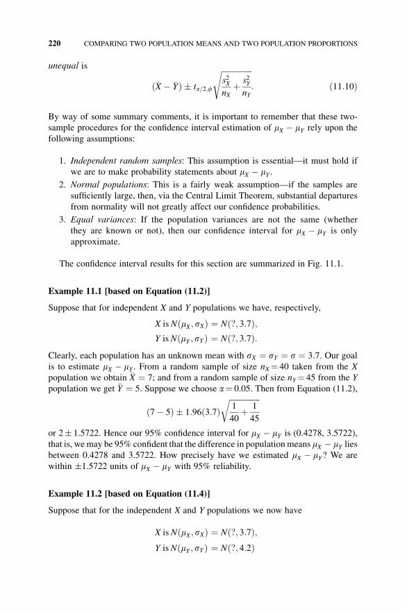
unequal is
�X � �Yð Þ � ta=2;f
ffiffiffiffiffiffiffiffiffiffiffiffiffiffiffiffis2XnX
þ s2YnY
s
: ð11:10Þ
By way of some summary comments, it is important to remember that these two-
sample procedures for the confidence interval estimation of mX � mY rely upon the
following assumptions:
1. Independent random samples: This assumption is essential—it must hold if
we are to make probability statements about mX � mY .2. Normal populations: This is a fairly weak assumption—if the samples are
sufficiently large, then, via the Central Limit Theorem, substantial departures
from normality will not greatly affect our confidence probabilities.
3. Equal variances: If the population variances are not the same (whether
they are known or not), then our confidence interval for mX � mY is only
approximate.
The confidence interval results for this section are summarized in Fig. 11.1.
Example 11.1 [based on Equation (11.2)]
Suppose that for independent X and Y populations we have, respectively,
X is NðmX ; sXÞ ¼ Nð?; 3:7Þ;Y isNðmY ; sYÞ ¼ Nð?; 3:7Þ:
Clearly, each population has an unknown mean with sX ¼ sY ¼ s ¼ 3:7. Our goalis to estimate mX � mY . From a random sample of size nX¼ 40 taken from the X
population we obtain �X ¼ 7; and from a random sample of size nY¼ 45 from the Y
population we get �Y ¼ 5. Suppose we choose a¼ 0.05. Then from Equation (11.2),
7� 5ð Þ � 1:96ð3:7Þffiffiffiffiffiffiffiffiffiffiffiffiffiffiffiffi1
40þ 1
45
r
or 2� 1.5722. Hence our 95% confidence interval for mX � mY is (0.4278, 3.5722),
that is, wemay be 95% confident that the difference in population means mX � mY liesbetween 0.4278 and 3.5722. How precisely have we estimated mX � mY? We are
within �1.5722 units of mX � mY with 95% reliability.
Example 11.2 [based on Equation (11.4)]
Suppose that for the independent X and Y populations we now have
X is NðmX ; sXÞ ¼ Nð?; 3:7Þ;Y isNðmY ; sYÞ ¼ Nð?; 4:2Þ
220 COMPARING TWO POPULATION MEANS AND TWO POPULATION PROPORTIONS
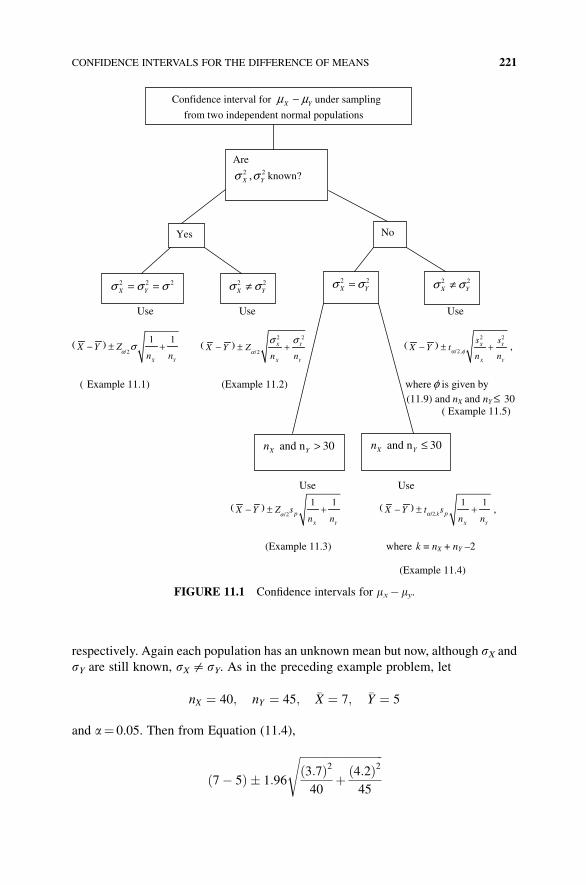
respectively. Again each population has an unknown mean but now, although sX andsY are still known, sX$ sY. As in the preceding example problem, let
nX ¼ 40; nY ¼ 45; �X ¼ 7; �Y ¼ 5
and a¼ 0.05. Then from Equation (11.4),
7� 5ð Þ � 1:96
ffiffiffiffiffiffiffiffiffiffiffiffiffiffiffiffiffiffiffiffiffiffiffiffiffiffiffiffiffiffið3:7Þ240
þ ð4:2Þ245
s
Use Use Use
( )α/2
1 1
X Y
X Y Zn n
σ− ± + ( )2 2 2 2
α/2X Y
X Y
X Y Zn n
σ σ− ± + ( )
α/2 ,φX Y
X Y
s sX Y t
n n− ± + ,
( Example 11.1) (Example 11.2) φ is given by where
where
(11.9) and nX and nY ≤ 30 ( Example 11.5)
Use Use
( )/2
1 1
X Y
pX Y Z sn n
α− ± + ( )α/2,
1 1k
X Y
pX Y t sn n
− ± + ,
(Example 11.3) k = nX + nY –2
(Example 11.4)
Confidence interval for X Yμ μ− under sampling
from two independent normal populations
Are2 2,X Yσ σ known?
Yes No
2 2 2X Yσ σ σ= = 2 2
X Yσ σ≠ 2 2X Yσ σ= 2 2
X Yσ σ≠
and n 30X Yn > and n 30X Yn ≤
FIGURE 11.1 Confidence intervals for mx� my.
CONFIDENCE INTERVALS FOR THE DIFFERENCE OF MEANS 221
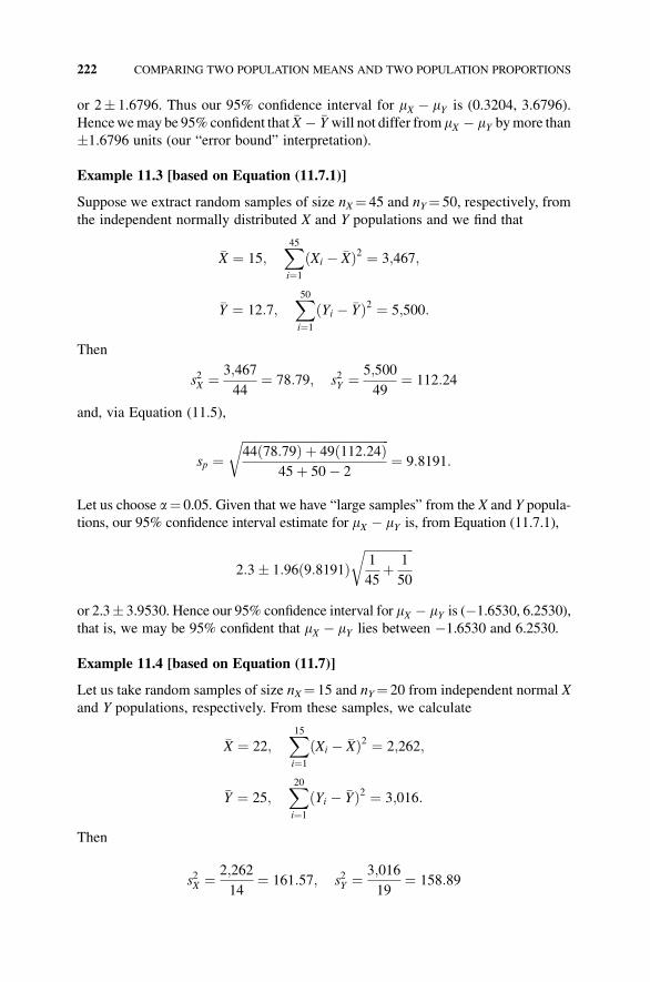
or 2� 1.6796. Thus our 95% confidence interval for mX � mY is (0.3204, 3.6796).
Hencewemay be 95% confident that �X � �Y will not differ from mX � mY bymore than
�1.6796 units (our “error bound” interpretation).
Example 11.3 [based on Equation (11.7.1)]
Suppose we extract random samples of size nX¼ 45 and nY¼ 50, respectively, from
the independent normally distributed X and Y populations and we find that
�X ¼ 15;X45
i¼1
ðXi � �XÞ2 ¼ 3;467;
�Y ¼ 12:7;X50
i¼1
ðYi � �YÞ2 ¼ 5;500:
Then
s2X ¼ 3;467
44¼ 78:79; s2Y ¼ 5;500
49¼ 112:24
and, via Equation (11.5),
sp ¼ffiffiffiffiffiffiffiffiffiffiffiffiffiffiffiffiffiffiffiffiffiffiffiffiffiffiffiffiffiffiffiffiffiffiffiffiffiffiffiffiffiffiffiffiffiffiffiffi44ð78:79Þ þ 49ð112:24Þ
45þ 50� 2
r¼ 9:8191:
Let us choose a¼ 0.05. Given that we have “large samples” from the X and Y popula-
tions, our 95% confidence interval estimate for mX � mY is, from Equation (11.7.1),
2:3� 1:96ð9:8191Þffiffiffiffiffiffiffiffiffiffiffiffiffiffiffiffi1
45þ 1
50
r
or 2.3� 3.9530. Hence our 95% confidence interval for mX � mY is (�1.6530, 6.2530),
that is, we may be 95% confident that mX � mY lies between �1.6530 and 6.2530.
Example 11.4 [based on Equation (11.7)]
Let us take random samples of size nX¼ 15 and nY¼ 20 from independent normal X
and Y populations, respectively. From these samples, we calculate
�X ¼ 22;X15
i¼1
ðXi � �XÞ2 ¼ 2;262;
�Y ¼ 25;X20
i¼1
ðYi � �YÞ2 ¼ 3;016:
Then
s2X ¼ 2;262
14¼ 161:57; s2Y ¼ 3;016
19¼ 158:89
222 COMPARING TWO POPULATION MEANS AND TWO POPULATION PROPORTIONS
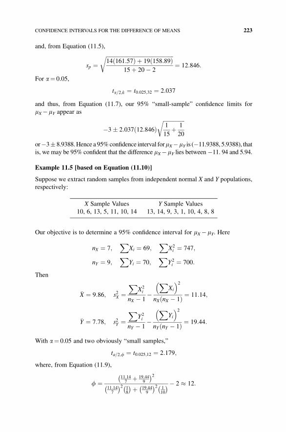
and, from Equation (11.5),
sp ¼ffiffiffiffiffiffiffiffiffiffiffiffiffiffiffiffiffiffiffiffiffiffiffiffiffiffiffiffiffiffiffiffiffiffiffiffiffiffiffiffiffiffiffiffiffiffiffiffiffiffi14ð161:57Þ þ 19ð158:89Þ
15þ 20� 2
r¼ 12:846:
For a¼ 0.05,
ta=2;k ¼ t0:025;32 ¼ 2:037
and thus, from Equation (11.7), our 95% “small-sample” confidence limits for
mX� mY appear as
�3� 2:037ð12:846Þffiffiffiffiffiffiffiffiffiffiffiffiffiffiffiffi1
15þ 1
20
r
or�3� 8.9388.Hence a 95%confidence interval formX� mY is (�11.9388, 5.9388), that
is, we may be 95% confident that the difference mX� mY lies between�11. 94 and 5.94.
Example 11.5 [based on Equation (11.10)]
Suppose we extract random samples from independent normal X and Y populations,
respectively:
X Sample Values Y Sample Values
10, 6, 13, 5, 11, 10, 14 13, 14, 9, 3, 1, 10, 4, 8, 8
Our objective is to determine a 95% confidence interval for mX� mY. Here
nX ¼ 7;X
Xi ¼ 69;X
X2i ¼ 747;
nY ¼ 9;X
Yi ¼ 70;X
Y2i ¼ 700:
Then
�X ¼ 9:86; s2X ¼X
X2i
nX � 1�
XXi
� �2
nXðnX � 1Þ ¼ 11:14;
�Y ¼ 7:78; s2Y ¼X
Y2i
nY � 1�
XYi
� �2
nYðnY � 1Þ ¼ 19:44:
With a¼ 0.05 and two obviously “small samples,”
ta=2;f ¼ t0:025;12 ¼ 2:179;
where, from Equation (11.9),
f ¼11:147
þ 19:449
� �2
11:147
� �2 18
� �þ 19:449
� �2 110
� �� 2 � 12:
CONFIDENCE INTERVALS FOR THE DIFFERENCE OF MEANS 223
Then from Equation (11.10), a 95% confidence interval for mX� mY is
2:08� 2:179
ffiffiffiffiffiffiffiffiffiffiffiffiffiffiffiffiffiffiffiffiffiffiffiffiffiffiffiffi11:14
7þ 19:44
9
r
or 2.08� 4.243. Hence we may be 95% confident that mX� mY lies within the interval(–2.163, 6.323). How precisely have we estimated mX� mY? We are within �4.243
units of mX� mY with 95% reliability. Alternatively stated, we may be 95% confident
that �X � �Y will not differ from mX� mY by more than �4.243 units.
11.2 CONFIDENCE INTERVALS FOR THE DIFFERENCE OF MEANSWHEN SAMPLING FROM TWO DEPENDENT POPULATIONS: PAIRED
COMPARISONS
The inferential techniques developed in the preceding section were based upon
random samples taken from two “independent” normal populations. What approach
should be taken when the samples are either intrinsically or purposefully designed to
be “dependent?” A common source of dependence is when the samples from the two
populations are paired—each observation in the first sample is related in some
particular way to exactly one observation in the second sample, so that the two
samples are obviously not independent.
Why is pairing advantageous? A glance back at, say, Equation (11.7) reveals
that the precision of the interval estimate of mX� mY, for fixed sample sizes nX and
nY, varies inversely with s2p, the pooled estimate of the common variance s2. Heres2p serves as a measure of the unexplained variation among experimental units or
subjects that receive similar treatments. One way to possibly reduce this variation,
and thus increase the precision of our estimate of mX� mY, is to pair the sample
observations. In this regard, if the variation in the treatment outcomes between the
members of any pair is less than the variation between corresponding members of
different pairs, then the precision of our estimate of mX� mY can be enhanced. And
this can be accomplished by randomizing the two treatments over the two members
of each pair in a fashion such that each treatment is applied to one and only one
member of each pair. The result of this paired experiment is that we can obtain, for
each pair of outcomes, an estimate of the difference between treatment effects, and
thus variation between pairs is not included in our estimate of the common
variance.
For instance, measurements are taken from the same experimental units at two
different points in time and the means of each set of measurements are subsequently
compared. In this regard, suppose a researcher conducts a before and afterweighing of
a group of people to determine the effectiveness of a new diet pill. Here the weights
will be paired—for a particular individual, his/her weight at the start of the
experiment (this measurement is an observation in the first sample) will be compared
to his/her weight at the end of the experiment (this latter data point is a member of the
second sample). Or experimental units in the two samples may be paired to eliminate
224 COMPARING TWO POPULATION MEANS AND TWO POPULATION PROPORTIONS
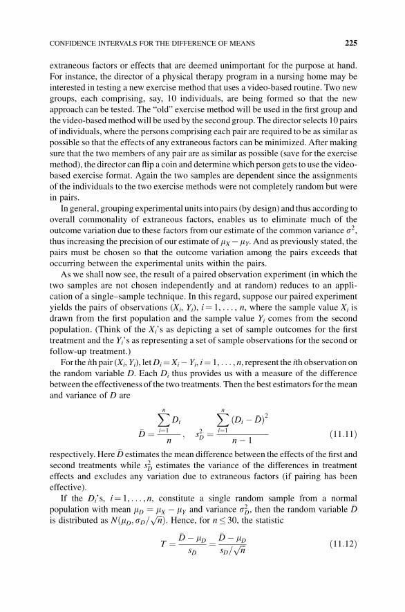
extraneous factors or effects that are deemed unimportant for the purpose at hand.
For instance, the director of a physical therapy program in a nursing home may be
interested in testing a new exercise method that uses a video-based routine. Two new
groups, each comprising, say, 10 individuals, are being formed so that the new
approach can be tested. The “old” exercise method will be used in the first group and
thevideo-basedmethodwill be used by the second group. The director selects 10 pairs
of individuals, where the persons comprising each pair are required to be as similar as
possible so that the effects of any extraneous factors can be minimized. After making
sure that the two members of any pair are as similar as possible (save for the exercise
method), the director can flip a coin and determinewhich person gets to use the video-
based exercise format. Again the two samples are dependent since the assignments
of the individuals to the two exercise methods were not completely random but were
in pairs.
In general, grouping experimental units into pairs (by design) and thus according to
overall commonality of extraneous factors, enables us to eliminate much of the
outcome variation due to these factors from our estimate of the common variance s2,thus increasing the precision of our estimate of mX� mY. And as previously stated, thepairs must be chosen so that the outcome variation among the pairs exceeds that
occurring between the experimental units within the pairs.
As we shall now see, the result of a paired observation experiment (in which the
two samples are not chosen independently and at random) reduces to an appli-
cation of a single–sample technique. In this regard, suppose our paired experiment
yields the pairs of observations (Xi, Yi), i¼ 1, . . . , n, where the sample value Xi is
drawn from the first population and the sample value Yi comes from the second
population. (Think of the Xi’s as depicting a set of sample outcomes for the first
treatment and the Yi’s as representing a set of sample observations for the second or
follow-up treatment.)
For the ith pair (Xi,Yi), letDi¼Xi� Yi, i¼ 1, . . . , n, represent the ith observation onthe random variable D. Each Di thus provides us with a measure of the difference
between the effectiveness of the two treatments. Then the best estimators for themean
and variance of D are
�D ¼
Xn
i¼1
Di
n; s2D ¼
Xn
i¼1
Di � �Dð Þ2
n� 1ð11:11Þ
respectively. Here �D estimates the mean difference between the effects of the first and
second treatments while s2D estimates the variance of the differences in treatment
effects and excludes any variation due to extraneous factors (if pairing has been
effective).
If the Di’s, i¼ 1, . . . , n, constitute a single random sample from a normal
population with mean mD ¼ mX � mY and variance s2D, then the random variable �Dis distributed as N mD; sD=
ffiffiffin
pð Þ. Hence, for n� 30, the statistic
T ¼�D� mDs�D
¼�D� mDsD=
ffiffiffin
p ð11:12Þ
CONFIDENCE INTERVALS FOR THE DIFFERENCE OF MEANS 225
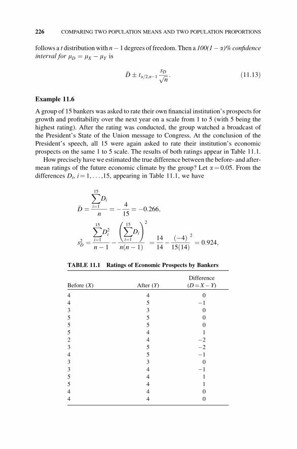
follows a t distributionwith n� 1 degrees of freedom. Then a 100(1� a)% confidence
interval for mD ¼ mX � mY is
�D� ta=2;n�1
sDffiffiffin
p : ð11:13Þ
Example 11.6
A group of 15 bankers was asked to rate their own financial institution’s prospects for
growth and profitability over the next year on a scale from 1 to 5 (with 5 being the
highest rating). After the rating was conducted, the group watched a broadcast of
the President’s State of the Union message to Congress. At the conclusion of the
President’s speech, all 15 were again asked to rate their institution’s economic
prospects on the same 1 to 5 scale. The results of both ratings appear in Table 11.1.
Howprecisely havewe estimated the true difference between the before- and after-
mean ratings of the future economic climate by the group? Let a¼ 0.05. From the
differences Di, i¼ 1, . . . ,15, appearing in Table 11.1, we have
�D ¼
X15
i¼1
Di
n¼ � 4
15¼ �0:266;
s2D ¼
X15
i¼1
D2i
n� 1�
X15
i¼1
Di
!
n n� 1ð Þ
2
¼ 14
14� �4ð Þ15 14ð Þ
2
¼ 0:924;
TABLE 11.1 Ratings of Economic Prospects by Bankers
Before (X) After (Y)
Difference
(D¼X� Y)
4 4 0
4 5 �1
3 3 0
5 5 0
5 5 0
5 4 1
2 4 �2
3 5 �2
4 5 �1
3 3 0
3 4 �1
5 4 1
5 4 1
4 4 0
4 4 0
226 COMPARING TWO POPULATION MEANS AND TWO POPULATION PROPORTIONS
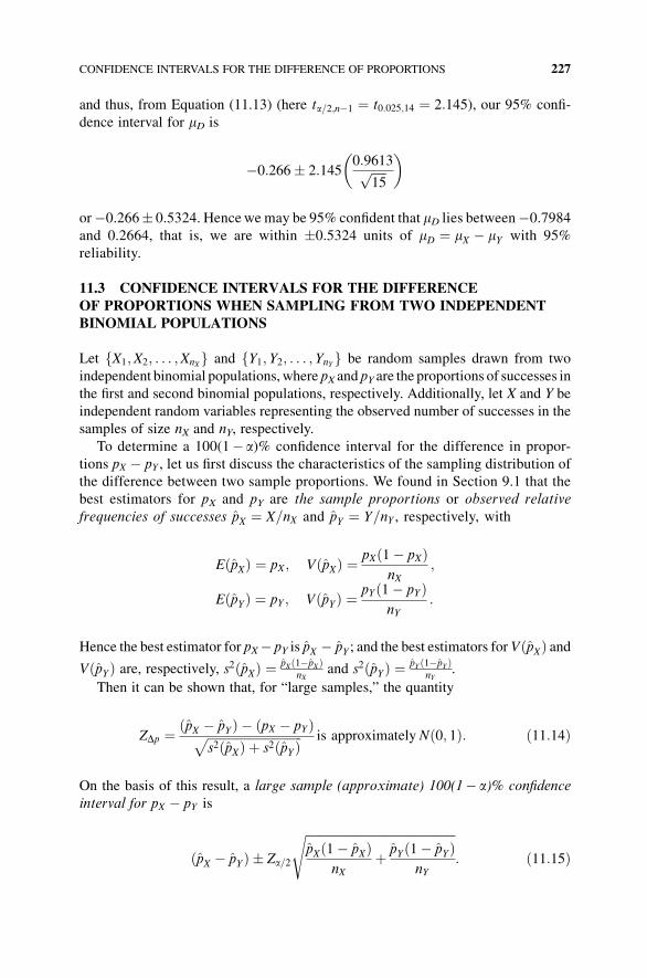
and thus, from Equation (11.13) (here ta=2;n�1 ¼ t0:025;14 ¼ 2:145), our 95% confi-
dence interval for mD is
�0:266� 2:1450:9613ffiffiffiffiffi
15p
� �
or�0.266� 0.5324. Hencewe may be 95% confident that mD lies between�0.7984
and 0.2664, that is, we are within �0.5324 units of mD ¼ mX � mY with 95%
reliability.
11.3 CONFIDENCE INTERVALS FOR THE DIFFERENCE
OF PROPORTIONS WHEN SAMPLING FROM TWO INDEPENDENTBINOMIAL POPULATIONS
Let X1;X2; . . . ;XnXf g and Y1; Y2; . . . ; YnYf g be random samples drawn from two
independent binomial populations, where pX and pY are the proportions of successes in
the first and second binomial populations, respectively. Additionally, let X and Y be
independent random variables representing the observed number of successes in the
samples of size nX and nY, respectively.
To determine a 100(1� a)% confidence interval for the difference in propor-
tions pX � pY , let us first discuss the characteristics of the sampling distribution of
the difference between two sample proportions. We found in Section 9.1 that the
best estimators for pX and pY are the sample proportions or observed relative
frequencies of successes pX ¼ X=nX and pY ¼ Y=nY , respectively, with
E pXð Þ ¼ pX ; V pXð Þ ¼ pX 1� pXð ÞnX
;
E pYð Þ ¼ pY ; V pYð Þ ¼ pY 1� pYð ÞnY
:
Hence the best estimator for pX� pY is pX � pY ; and the best estimators for VðpXÞ andVðpYÞ are, respectively, s2 pXð Þ ¼ pX 1�pXð Þ
nXand s2 pYð Þ ¼ pY 1�pYð Þ
nY.
Then it can be shown that, for “large samples,” the quantity
ZDp ¼ pX � pYð Þ � pX � pYð Þffiffiffiffiffiffiffiffiffiffiffiffiffiffiffiffiffiffiffiffiffiffiffiffiffiffiffiffiffiffiffis2 pXð Þ þ s2 pYð Þp is approximately Nð0; 1Þ: ð11:14Þ
On the basis of this result, a large sample (approximate) 100(1� a)% confidence
interval for pX � pY is
pX � pYð Þ � Za=2
ffiffiffiffiffiffiffiffiffiffiffiffiffiffiffiffiffiffiffiffiffiffiffiffiffiffiffiffiffiffiffiffiffiffiffiffiffiffiffiffiffiffiffiffiffiffiffiffiffipX 1� pXð Þ
nXþ pY 1� pYð Þ
nY
s
: ð11:15Þ
CONFIDENCE INTERVALS FOR THE DIFFERENCE OF PROPORTIONS 227
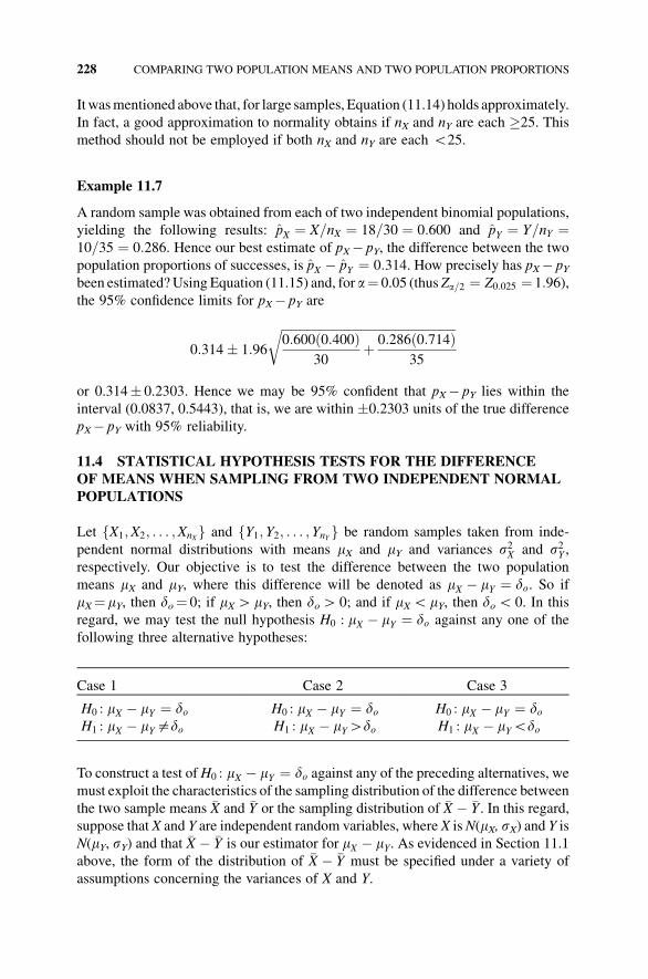
Itwasmentioned above that, for large samples, Equation (11.14) holds approximately.
In fact, a good approximation to normality obtains if nX and nY are each �25. This
method should not be employed if both nX and nY are each G25.
Example 11.7
A random sample was obtained from each of two independent binomial populations,
yielding the following results: pX ¼ X=nX ¼ 18=30 ¼ 0:600 and pY ¼ Y=nY ¼10=35 ¼ 0:286. Hence our best estimate of pX� pY, the difference between the two
population proportions of successes, is pX � pY ¼ 0:314. How precisely has pX� pYbeen estimated?Using Equation (11.15) and, for a¼ 0.05 (thus Za=2 ¼ Z0:025 ¼ 1:96),the 95% confidence limits for pX� pY are
0:314� 1:96
ffiffiffiffiffiffiffiffiffiffiffiffiffiffiffiffiffiffiffiffiffiffiffiffiffiffiffiffiffiffiffiffiffiffiffiffiffiffiffiffiffiffiffiffiffiffiffiffiffiffiffiffiffiffiffiffiffi0:600ð0:400Þ
30þ 0:286ð0:714Þ
35
r
or 0.314� 0.2303. Hence we may be 95% confident that pX� pY lies within the
interval (0.0837, 0.5443), that is, we are within �0.2303 units of the true difference
pX� pY with 95% reliability.
11.4 STATISTICAL HYPOTHESIS TESTS FOR THE DIFFERENCE
OF MEANS WHEN SAMPLING FROM TWO INDEPENDENT NORMALPOPULATIONS
Let X1;X2; . . . ;XnXf g and Y1; Y2; . . . ; YnYf g be random samples taken from inde-
pendent normal distributions with means mX and mY and variances s2X and s2Y ,respectively. Our objective is to test the difference between the two population
means mX and mY, where this difference will be denoted as mX � mY ¼ do. So if
mX¼ mY, then do¼ 0; if mXH mY, then doH 0; and if mXG mY, then doG 0. In this
regard, we may test the null hypothesis H0 : mX � mY ¼ do against any one of the
following three alternative hypotheses:
Case 1 Case 2 Case 3
H0 : mX � mY ¼ do H0 : mX � mY ¼ do H0 : mX � mY ¼ doH1 : mX � mY$do H1 : mX � mYHdo H1 : mX � mYGdo
To construct a test ofH0 : mX � mY ¼ do against any of the preceding alternatives, wemust exploit the characteristics of the sampling distribution of the difference between
the two sample means �X and �Y or the sampling distribution of �X � �Y . In this regard,suppose that X and Y are independent random variables, where X isN(mX, sX) and Y is
N(mY, sY) and that �X � �Y is our estimator for mX � mY. As evidenced in Section 11.1
above, the form of the distribution of �X � �Y must be specified under a variety of
assumptions concerning the variances of X and Y.
228 COMPARING TWO POPULATION MEANS AND TWO POPULATION PROPORTIONS
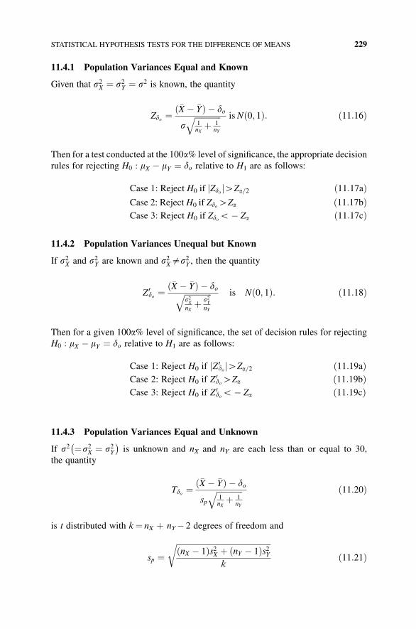
11.4.1 Population Variances Equal and Known
Given that s2X ¼ s2Y ¼ s2 is known, the quantity
Zdo ¼ð�X � �YÞ � do
sffiffiffiffiffiffiffiffiffiffiffiffiffi1nXþ 1
nY
q isNð0; 1Þ: ð11:16Þ
Then for a test conducted at the 100a% level of significance, the appropriate decision
rules for rejecting H0 : mX � mY ¼ do relative to H1 are as follows:
Case 1: Reject H0 if Zdoj jHZa=2 ð11:17aÞCase 2: Reject H0 if ZdoHZa ð11:17bÞCase 3: Reject H0 if ZdoG� Za ð11:17cÞ
11.4.2 Population Variances Unequal but Known
If s2X and s2Y are known and s2X$s2Y , then the quantity
Z 0do ¼
ð�X � �YÞ � doffiffiffiffiffiffiffiffiffiffiffiffiffiffis2X
nXþ s2
Y
nY
q is Nð0; 1Þ: ð11:18Þ
Then for a given 100a% level of significance, the set of decision rules for rejecting
H0 : mX � mY ¼ do relative to H1 are as follows:
Case 1: Reject H0 if Z 0doj jHZa=2 ð11:19aÞ
Case 2: Reject H0 if Z0doHZa ð11:19bÞ
Case 3: Reject H0 if Z0doG� Za ð11:19cÞ
11.4.3 Population Variances Equal and Unknown
If s2 ¼s2X ¼ s2Y� �
is unknown and nX and nY are each less than or equal to 30,
the quantity
Tdo ¼ð�X � �YÞ � do
sp
ffiffiffiffiffiffiffiffiffiffiffiffiffi1nXþ 1
nY
q ð11:20Þ
is t distributed with k¼ nX þ nY� 2 degrees of freedom and
sp ¼ffiffiffiffiffiffiffiffiffiffiffiffiffiffiffiffiffiffiffiffiffiffiffiffiffiffiffiffiffiffiffiffiffiffiffiffiffiffiffiffiffiffiffiffiffiffiffiffinX � 1ð Þs2X þ nY � 1ð Þs2Y
k
rð11:21Þ
STATISTICAL HYPOTHESIS TESTS FOR THE DIFFERENCE OF MEANS 229
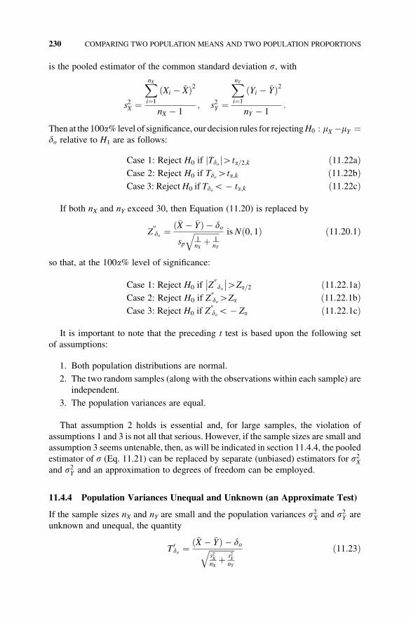
is the pooled estimator of the common standard deviation s, with
s2X ¼
XnX
i¼1
Xi � �Xð Þ2
nX � 1; s2Y ¼
XnY
i¼1
Yi � �Yð Þ2
nY � 1:
Then at the 100a%level of significance, our decision rules for rejectingH0 : mX �mY ¼do relative to H1 are as follows:
Case 1: Reject H0 if Tdoj jHta=2;k ð11:22aÞCase 2: Reject H0 if TdoHta;k ð11:22bÞCase 3: Reject H0 if TdoG� ta;k ð11:22cÞ
If both nX and nY exceed 30, then Equation (11.20) is replaced by
Z00do ¼
ð�X � �YÞ � do
sp
ffiffiffiffiffiffiffiffiffiffiffiffiffi1nXþ 1
nY
q is Nð0; 1Þ ð11:20:1Þ
so that, at the 100a% level of significance:
Case 1: Reject H0 if Z00do
HZa=2 ð11:22:1aÞCase 2: Reject H0 if Z
00doHZa ð11:22:1bÞ
Case 3: Reject H0 if Z00doG� Za ð11:22:1cÞ
It is important to note that the preceding t test is based upon the following set
of assumptions:
1. Both population distributions are normal.
2. The two random samples (along with the observations within each sample) are
independent.
3. The population variances are equal.
That assumption 2 holds is essential and, for large samples, the violation of
assumptions 1 and 3 is not all that serious. However, if the sample sizes are small and
assumption 3 seems untenable, then, as will be indicated in section 11.4.4, the pooled
estimator of s (Eq. 11.21) can be replaced by separate (unbiased) estimators for s2Xand s2Y and an approximation to degrees of freedom can be employed.
11.4.4 Population Variances Unequal and Unknown (an Approximate Test)
If the sample sizes nX and nY are small and the population variances s2X and s2Y are
unknown and unequal, the quantity
T 0do ¼
ð�X � �YÞ � doffiffiffiffiffiffiffiffiffiffiffiffiffis2X
nXþ s2
Y
nY
q ð11:23Þ
230 COMPARING TWO POPULATION MEANS AND TWO POPULATION PROPORTIONS
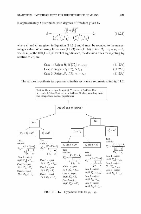
is approximately t distributed with degrees of freedom given by
f ¼s2XnXþ s2Y
nY
� �2
s2X
nX
� �21
nXþ1
� �þ s2
Y
nY
� �21
nYþ1
� �� 2; ð11:24Þ
where s2X and s2Y are given in Equation (11.21) and f must be rounded to the nearest
integer value. When using Equations (11.23) and (11.24) to test Ho : mX � mY ¼ doversusH1 at the 100(1� a)% level of significance, the decision rules for rejecting H0
relative to H1 are:
Case 1: Reject H0 if T 0doj jHta=2;f ð11:25aÞ
Case 2: Reject H0 if T0doHta;f ð11:25bÞ
Case 3: Reject H0 if T0doG� ta;f ð11:25cÞ
The various hypothesis tests presented in this section are summarized in Fig. 11.2.
Test for H0: μX – μY = δ0 against H1: μX – μY ≠ δ 0 (Case 1) or μX – μY > δ 0(Case 2) or μX – μY < δ0(Case 3) when sampling from two independent normal populations
Are 2Xσ and 2
Yσ known?
No Yes
22
YXσ σ≠
Test statistic:
2 2
( )o
0
X Y
X Y
X YT
s s
n n
δ
δ− −′ =
+
Case 1 – reject H0 if /2,0
T tδ α φ′ >Case 2 – reject H0 if ,0
T tδ α φ′ >Case 3 – reject H0 if ,0
T tδ α φ′ < −
Test statistic:
2 2
( )0
0
X Y
X Y
X YZ
n n
δ
δ
σ σ
− −′ =
+
Case 1 – reject H0 if /20
Z Zδ α′ >Case 2 – reject H0 if 0
Z Zδ α′ >Case 3 – reject H0 if 0
Z Zδ α′ < − .
2 2X Yσ σ≠
Test statistic:
( )
1 10
0
X Y
X YZ
n n
δ
δ
σ
− −=
+
Case 1 – reject H0 if /20
Z Zδ α>Case 2 – reject H0 if 0
Z Zδ α>Case 3 – reject H0 if 0
Z Zδ α< −
2 2 2X Yσ σ σ= =
2 2X Yσ σ=
Test statistic:
( )
1 10
0
p
X Y
X YZ
sn n
δ
δ− −″ =+
Case 1 – reject H0 if /20
Z Zδ α″ >Case 2 – reject H0 if 0
Z Zδ α″ >Case 3 – reject H0 if 0
Z Zδ α″ < −
nX and nY < 30
Test statistic:
( )
1 10
0
p
X Y
X YT
sn n
δ
δ− −=
+
Case 1 – reject H0 if /2,0 kT tδ α> ;
Case 2 – reject H0 if ,0 kT tδ α> ;
Case 3 – reject H0 if ,0 kT tδ α< − .
nX and nY > 30
FIGURE 11.2 Hypothesis tests for mx� my.
STATISTICAL HYPOTHESIS TESTS FOR THE DIFFERENCE OF MEANS 231
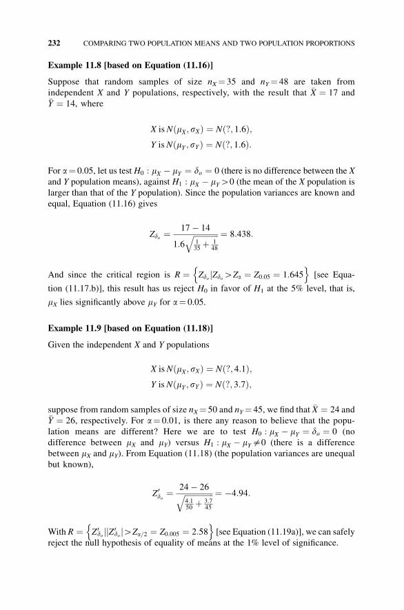
Example 11.8 [based on Equation (11.16)]
Suppose that random samples of size nX¼ 35 and nY¼ 48 are taken from
independent X and Y populations, respectively, with the result that �X ¼ 17 and�Y ¼ 14, where
X is NðmX; sXÞ ¼ Nð?; 1:6Þ;Y is NðmY ; sYÞ ¼ Nð?; 1:6Þ:
For a¼ 0.05, let us test H0 : mX � mY ¼ do ¼ 0 (there is no difference between the X
and Y population means), against H1 : mX � mYH0 (the mean of the X population is
larger than that of the Y population). Since the population variances are known and
equal, Equation (11.16) gives
Zdo ¼17� 14
1:6ffiffiffiffiffiffiffiffiffiffiffiffiffi135þ 1
48
q ¼ 8:438:
And since the critical region is R ¼ Zdo jZdoHZa ¼ Z0:05 ¼ 1:645n o
[see Equa-
tion (11.17.b)], this result has us reject H0 in favor of H1 at the 5% level, that is,
mX lies significantly above mY for a¼ 0.05.
Example 11.9 [based on Equation (11.18)]
Given the independent X and Y populations
X isNðmX; sXÞ ¼ Nð?; 4:1Þ;Y is NðmY ; sYÞ ¼ Nð?; 3:7Þ;
suppose from random samples of size nX¼ 50 and nY¼ 45, we find that �X ¼ 24 and�Y ¼ 26, respectively. For a¼ 0.01, is there any reason to believe that the popu-
lation means are different? Here we are to test H0 : mX � mY ¼ do ¼ 0 (no
difference between mX and mY) versus H1 : mX � mY$0 (there is a difference
between mX and mY). From Equation (11.18) (the population variances are unequal
but known),
Z 0do ¼
24� 26ffiffiffiffiffiffiffiffiffiffiffiffiffiffiffi4:150
þ 3:745
q ¼ �4:94:
With R ¼ Z 0do jjZ 0
do jHZa=2 ¼ Z0:005 ¼ 2:58n o
[see Equation (11.19a)], we can safely
reject the null hypothesis of equality of means at the 1% level of significance.
232 COMPARING TWO POPULATION MEANS AND TWO POPULATION PROPORTIONS
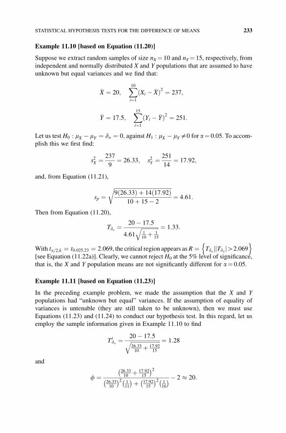
Example 11.10 [based on Equation (11.20)]
Suppose we extract random samples of size nX¼ 10 and nY¼ 15, respectively, from
independent and normally distributed X and Y populations that are assumed to have
unknown but equal variances and we find that:
�X ¼ 20;X10
i¼1
Xi � �Xð Þ2 ¼ 237;
�Y ¼ 17:5;X15
i¼1
Yi � �Yð Þ2 ¼ 251:
Let us test H0 : mX � mY ¼ do ¼ 0; against H1 : mX � mY$0 for a¼ 0.05. To accom-
plish this we first find:
s2X ¼ 237
9¼ 26:33; s2Y ¼ 251
14¼ 17:92;
and, from Equation (11.21),
sp ¼ffiffiffiffiffiffiffiffiffiffiffiffiffiffiffiffiffiffiffiffiffiffiffiffiffiffiffiffiffiffiffiffiffiffiffiffiffiffiffiffiffiffiffi9ð26:33Þ þ 14ð17:92Þ
10þ 15� 2
r¼ 4:61:
Then from Equation (11.20),
Tdo ¼20� 17:5
4:61ffiffiffiffiffiffiffiffiffiffiffiffiffi110þ 1
15
q ¼ 1:33:
With ta=2;k ¼ t0:025;23 ¼ 2:069, the critical region appears asR ¼ Tdo jjTdo jH2:069n o
[see Equation (11.22a)]. Clearly, we cannot reject H0 at the 5% level of significance,
that is, the X and Y population means are not significantly different for a¼ 0.05.
Example 11.11 [based on Equation (11.23)]
In the preceding example problem, we made the assumption that the X and Y
populations had “unknown but equal” variances. If the assumption of equality of
variances is untenable (they are still taken to be unknown), then we must use
Equations (11.23) and (11.24) to conduct our hypothesis test. In this regard, let us
employ the sample information given in Example 11.10 to find
T 0do ¼
20� 17:5ffiffiffiffiffiffiffiffiffiffiffiffiffiffiffiffiffiffiffiffiffiffi26:3310
þ 17:9215
q ¼ 1:28
and
f ¼26:3310
þ 17:9215
� �2
26:3310
� �2 111
� �þ 17:9215
� �2 116
� �� 2 � 20:
STATISTICAL HYPOTHESIS TESTS FOR THE DIFFERENCE OF MEANS 233
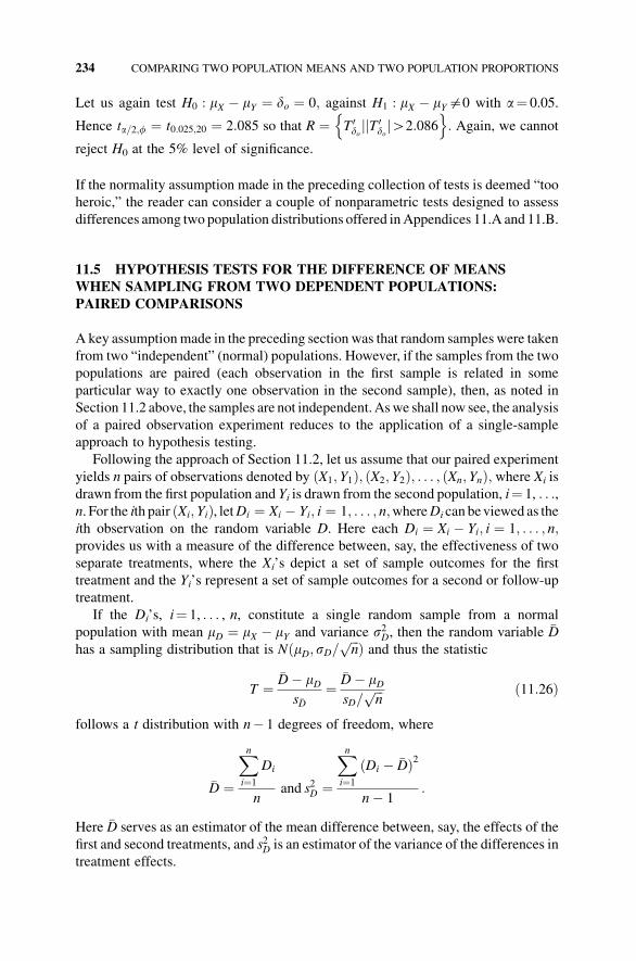
Let us again test H0 : mX � mY ¼ do ¼ 0; against H1 : mX � mY$0 with a¼ 0.05.
Hence ta=2;f ¼ t0:025;20 ¼ 2:085 so that R ¼ T 0do jjT 0
do jH2:086n o
: Again, we cannot
reject H0 at the 5% level of significance.
If the normality assumption made in the preceding collection of tests is deemed “too
heroic,” the reader can consider a couple of nonparametric tests designed to assess
differences among two population distributions offered inAppendices 11.A and 11.B.
11.5 HYPOTHESIS TESTS FOR THE DIFFERENCE OF MEANSWHEN SAMPLING FROM TWO DEPENDENT POPULATIONS:
PAIRED COMPARISONS
Akey assumptionmade in the preceding section was that random samples were taken
from two “independent” (normal) populations. However, if the samples from the two
populations are paired (each observation in the first sample is related in some
particular way to exactly one observation in the second sample), then, as noted in
Section 11.2 above, the samples are not independent.Aswe shall now see, the analysis
of a paired observation experiment reduces to the application of a single-sample
approach to hypothesis testing.
Following the approach of Section 11.2, let us assume that our paired experiment
yields n pairs of observations denoted by X1; Y1ð Þ; X2; Y2ð Þ; . . . ; Xn; Ynð Þ; where Xi is
drawn from the first population and Yi is drawn from the second population, i¼ 1, . . .,n. For the ith pair Xi; Yið Þ, letDi ¼ Xi � Yi; i ¼ 1; . . . ; n;whereDi can beviewed as the
ith observation on the random variable D. Here each Di ¼ Xi � Yi; i ¼ 1; . . . ; n;provides us with a measure of the difference between, say, the effectiveness of two
separate treatments, where the Xi’s depict a set of sample outcomes for the first
treatment and the Yi’s represent a set of sample outcomes for a second or follow-up
treatment.
If the Di’s, i¼ 1, . . . , n, constitute a single random sample from a normal
population with mean mD ¼ mX � mY and variance s2D, then the random variable �Dhas a sampling distribution that is N mD; sD=
ffiffiffin
pð Þ and thus the statistic
T ¼�D� mDs�D
¼�D� mDsD=
ffiffiffin
p ð11:26Þ
follows a t distribution with n� 1 degrees of freedom, where
�D ¼
Xn
i¼1
Di
nand s2D ¼
Xn
i¼1
Di � �Dð Þ2
n� 1:
Here �D serves as an estimator of the mean difference between, say, the effects of the
first and second treatments, and s2D is an estimator of the variance of the differences in
treatment effects.
234 COMPARING TWO POPULATION MEANS AND TWO POPULATION PROPORTIONS
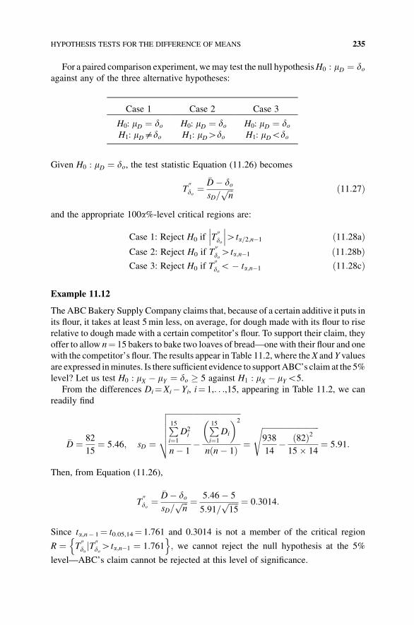
For a paired comparison experiment, wemay test the null hypothesisH0 : mD ¼ doagainst any of the three alternative hypotheses:
Case 1 Case 2 Case 3
H0: mD ¼ do H0: mD ¼ do H0: mD ¼ doH1: mD$do H1: mDHdo H1: mDGdo
Given H0 : mD ¼ do, the test statistic Equation (11.26) becomes
T00do ¼
�D� dosD=
ffiffiffin
p ð11:27Þ
and the appropriate 100a%-level critical regions are:
Case 1: Reject H0 if T00do
Hta=2;n�1 ð11:28aÞ
Case 2: Reject H0 if T00doHta;n�1 ð11:28bÞ
Case 3: Reject H0 if T00doG� ta;n�1 ð11:28cÞ
Example 11.12
TheABCBakery Supply Company claims that, because of a certain additive it puts in
its flour, it takes at least 5min less, on average, for dough made with its flour to rise
relative to dough made with a certain competitor’s flour. To support their claim, they
offer to allow n¼ 15 bakers to bake two loaves of bread—onewith their flour and one
with the competitor’s flour. The results appear in Table 11.2, where theX and Y values
are expressed inminutes. Is there sufficient evidence to supportABC’s claim at the 5%
level? Let us test H0 : mX � mY ¼ do � 5 against H1 : mX � mYG5.
From the differences Di¼Xi� Yi, i¼ 1,. . .,15, appearing in Table 11.2, we can
readily find
�D ¼ 82
15¼ 5:46; sD ¼
ffiffiffiffiffiffiffiffiffiffiffiffiffiffiffiffiffiffiffiffiffiffiffiffiffiffiffiffiffiffiffiffiffiffiffiffiffiP15
i¼1
D2i
n� 1�
P15
i¼1
Di
� �2
nðn� 1Þ
vuuuut ¼ffiffiffiffiffiffiffiffiffiffiffiffiffiffiffiffiffiffiffiffiffiffiffiffiffiffiffiffiffi938
14� ð82Þ215� 14
s
¼ 5:91:
Then, from Equation (11.26),
T00do ¼
�D� dosD=
ffiffiffin
p ¼ 5:46� 5
5:91=ffiffiffiffiffi15
p ¼ 0:3014:
Since ta,n� 1¼ t0.05,14¼ 1.761 and 0.3014 is not a member of the critical region
R ¼ T00do jT
00doHta;n�1 ¼ 1:761
n o; we cannot reject the null hypothesis at the 5%
level—ABC’s claim cannot be rejected at this level of significance.
HYPOTHESIS TESTS FOR THE DIFFERENCE OF MEANS 235
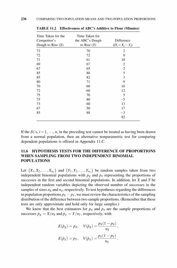
If the Di’s, i¼ 1, . . ., n, in the preceding test cannot be treated as having been drawnfrom a normal population, then an alternative nonparametric test for comparing
dependent populations is offered in Appendix 11.C.
11.6 HYPOTHESIS TESTS FOR THE DIFFERENCE OF PROPORTIONS
WHEN SAMPLING FROM TWO INDEPENDENT BINOMIALPOPULATIONS
Let X1;X2; . . . ;XnXf g and Y1; Y2; . . . ; YnYf g be random samples taken from two
independent binomial populations with pX and pY representing the proportions of
successes in the first and second binomial populations. In addition, let X and Y be
independent random variables depicting the observed number of successes in the
samples of sizes nX and nY, respectively. To test hypotheses regarding the differences
in population proportions pX � pY , wemust review the characteristics of the sampling
distribution of the difference between two sample proportions. (Remember that these
tests are only approximate and hold only for large samples.)
We know that the best estimators for pX and pY are the sample proportions of
successes pX ¼ X=nX and pY ¼ Y=nY , respectively, with
EðpXÞ ¼ pX; V pXð Þ ¼ pXð1� pXÞnX
;
EðpYÞ ¼ pY ; V pYð Þ ¼ pYð1� pYÞnY
:
TABLE 11.2 Effectiveness of ABC’s Additive to Flour (Minutes)
Time Taken for the
Competitor’s
Dough to Rise (X)
Time Taken for
the ABC’s Dough
to Rise (Y)
Difference
(Di¼Xi� Yi)
72 70 2
72 72 0
71 61 10
69 67 2
67 65 2
85 80 5
85 82 3
80 71 9
70 60 10
72 60 12
75 70 5
75 80 �5
73 60 13
67 50 17
85 88 �3
82
236 COMPARING TWO POPULATION MEANS AND TWO POPULATION PROPORTIONS
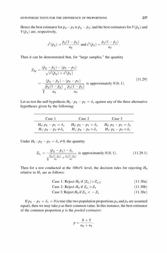
Hence the best estimator for pX� pY is pX � pY ; and the best estimators for VðpXÞ andVðpYÞ are, respectively,
s2 pXð Þ ¼ pX 1� pXð ÞnX
and s2 pYð Þ ¼ pY 1� pYð ÞnY
:
Then it can be demonstrated that, for “large samples,” the quantity
ZDp ¼ pX � pYð Þ � pX � pYð Þffiffiffiffiffiffiffiffiffiffiffiffiffiffiffiffiffiffiffiffiffiffiffiffiffiffiffiffiffiffiffis2 pXð Þ þ s2 pYð Þp
¼ ðpX � pYÞ � ðpX � pYÞffiffiffiffiffiffiffiffiffiffiffiffiffiffiffiffiffiffiffiffiffiffiffiffiffiffiffiffiffiffiffiffiffiffiffiffiffiffiffiffiffiffiffiffiffiffiffiffiffipXð1� pXÞ
nXþ pYð1� pYÞ
nY
r is approximately Nð0; 1Þ:ð11:29Þ
Let us test the null hypothesis H0 : pX � pY ¼ do against any of the three alternativehypotheses given by the following:
Case 1 Case 2 Case 3
H0: pX � pY ¼ do H0: pX � pY ¼ do H0: pX � pY ¼ doH1: pX � pY$do H1: pX � pYHdo H1: pX � pYGdo
Under H0 : pX � pY ¼ do$0, the quantity
Zdo ¼pX � pYð Þ � doffiffiffiffiffiffiffiffiffiffiffiffiffiffiffiffiffiffiffiffiffiffiffiffiffiffiffiffiffiffiffiffiffiffipXð1�pXÞ
nXþ pY ð1�pY Þ
nY
q is approximately Nð0; 1Þ: ð11:29:1Þ
Then for a test conducted at the 100a% level, the decision rules for rejecting H0
relative to H1 are as follows:
Case 1: Reject H0 if Zdoj jHZa=2 ð11:30aÞCase 2: Reject H0 if ZdoHZa ð11:30bÞCase 3: RejectH0 if ZdoG� Za ð11:30cÞ
If pX � pY ¼ do ¼ 0 is true (the two population proportions pX and pY are assumed
equal), then we may take p as their common value. In this instance, the best estimator
of the common proportion p is the pooled estimator:
p ¼ X þ Y
nX þ nY:
HYPOTHESIS TESTS FOR THE DIFFERENCE OF PROPORTIONS 237
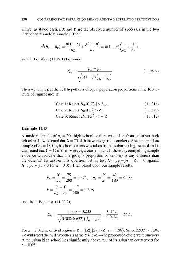
where, as stated earlier, X and Y are the observed number of successes in the two
independent random samples. Then
s2 pX � pYð Þ ¼ p 1� pð ÞnX
þ p 1� pð ÞnY
¼ pð1� pÞ 1
nXþ 1
nY
� �;
so that Equation (11.29.1) becomes
Z 0do ¼
pX � pYffiffiffiffiffiffiffiffiffiffiffiffiffiffiffiffiffiffiffiffiffiffiffiffiffiffiffiffiffiffiffiffiffiffiffiffipð1� pÞ 1
nXþ 1
nY
� �r : ð11:29:2Þ
Then we will reject the null hypothesis of equal population proportions at the 100a%level of significance if:
Case 1: Reject H0 if Z 0doj jHZa=2 ð11:31aÞ
Case 2: Reject H0 if Z0doHZa ð11:31bÞ
Case 3: Reject H0 if Z0doG� Za ð11:31cÞ
Example 11.13
A random sample of nX¼ 200 high school seniors was taken from an urban high
school and it was found thatX¼ 75 of themwere cigarette smokers. A second random
sample of nY¼ 180 high school seniors was taken from a suburban high school and it
was found thatY¼ 42 of themwere cigarette smokers. Is there any compelling sample
evidence to indicate that one group’s proportion of smokers is any different than
the other’s? To answer this question, let us test H0 : pX � pY ¼ do ¼ 0 against
H1 : pX � pY$0 for a¼ 0.05. Then based upon our sample results:
pX ¼ X
nX¼ 75
200¼ 0:375; pY ¼ Y
nY¼ 42
180¼ 0:233;
p ¼ X þ Y
nX þ nY¼ 117
380¼ 0:308
and, from Equation (11.29.2),
Z 0do ¼
0:375� 0:233ffiffiffiffiffiffiffiffiffiffiffiffiffiffiffiffiffiffiffiffiffiffiffiffiffiffiffiffiffiffiffiffiffiffiffiffiffiffiffiffiffiffiffiffiffiffi0:308 0:692ð Þ 1
200þ 1
180
� �q ¼ 0:142
0:0484¼ 2:933:
For a¼ 0.05, the critical region is R ¼ fZ 0do jZ 0
doHZa=2 ¼ 1:96g. Since 2.933H 1.96,
wewill reject the null hypothesis at the 5% level—the proportion of cigarette smokers
at the urban high school lies significantly above that of its suburban counterpart for
a¼ 0.05.
238 COMPARING TWO POPULATION MEANS AND TWO POPULATION PROPORTIONS
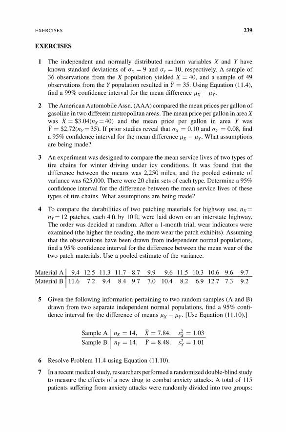
EXERCISES
1 The independent and normally distributed random variables X and Y have
known standard deviations of sx ¼ 9 and sy ¼ 10, respectively. A sample of
36 observations from the X population yielded �X ¼ 40, and a sample of 49
observations from the Y population resulted in �Y ¼ 35. Using Equation (11.4),
find a 99% confidence interval for the mean difference mX � mY .
2 TheAmericanAutomobileAssn. (AAA) compared themean prices per gallon of
gasoline in two different metropolitan areas. The mean price per gallon in area X
was �X ¼ $3:04(nX¼ 40) and the mean price per gallon in area Y was�Y ¼ $2:72(nY¼ 35). If prior studies reveal that sX ¼ 0:10 and sY ¼ 0:08, finda 95% confidence interval for the mean difference mX � mY . What assumptions
are being made?
3 An experiment was designed to compare the mean service lives of two types of
tire chains for winter driving under icy conditions. It was found that the
difference between the means was 2,250 miles, and the pooled estimate of
variance was 625,000. There were 20 chain sets of each type. Determine a 95%
confidence interval for the difference between the mean service lives of these
types of tire chains. What assumptions are being made?
4 To compare the durabilities of two patching materials for highway use, nX¼nY¼ 12 patches, each 4 ft by 10 ft, were laid down on an interstate highway.
The order was decided at random. After a 1-month trial, wear indicators were
examined (the higher the reading, the more wear the patch exhibits). Assuming
that the observations have been drawn from independent normal populations,
find a 95% confidence interval for the difference between the mean wear of the
two patch materials. Use a pooled estimate of the variance.
Material A 9.4 12.5 11.3 11.7 8.7 9.9 9.6 11.5 10.3 10.6 9.6 9.7
Material B 11.6 7.2 9.4 8.4 9.7 7.0 10.4 8.2 6.9 12.7 7.3 9.2
5 Given the following information pertaining to two random samples (A and B)
drawn from two separate independent normal populations, find a 95% confi-
dence interval for the difference of means mX � mY . [Use Equation (11.10).]
Sample A nX ¼ 14; �X ¼ 7:84; s2X ¼ 1:03
Sample B nY ¼ 14; �Y ¼ 8:48; s2Y ¼ 1:01
6 Resolve Problem 11.4 using Equation (11.10).
7 In a recentmedical study, researchers performed a randomized double-blind study
to measure the effects of a new drug to combat anxiety attacks. A total of 115
patients suffering from anxiety attacks were randomly divided into two groups:
EXERCISES 239
group 1 (the experimental group that generated the X values) received 10mg per
day of the drug, while group 2 (the control group that produced the Y values)
received the inert placebo. (Neither the subjects nor the researchers knewwhowas
in the experimental or control group—the double-blind property.) The effective-
ness of the drug was measured using a generally accepted scoring technique with
the net improvement in the score recorded. The results are presented below. Find a
95% confidence interval about mX � mY . Use Equation (11.10).
Group 1 nX ¼ 55; �X ¼ 14:89; s2X ¼ 156:25
Group 2 nY ¼ 60; �Y ¼ 8:17; s2Y ¼ 161:29
8 Determine whether the following sampling plans are independent or dependent:
a. A research team wishes to determine the effects of alcohol on a subject’s
reaction time to a flash of light. (When the light flashes, the subject presses a
button and his/her reaction time is recorded.) One hundred individuals of
legal drinking age are divided into two groups: group 1 subjects drink 3
ounces of alcoholwhile group 2 participants drink a placebo. Both drinks look
and taste the same and individuals participating in the study do not knowwho
gets the alcohol and who gets the placebo. Each person is given 1min to
consume the drink and 30min later the reaction times of the subjects in each
group are recorded.
b. The local Grange wants to determine if there is any significant improvement
in crop yield due to the application of a new pesticide. They divide a large plot
of land with uniform soil quality into 40 subplots. They then randomly
selected 20 plots to be sprayed with the new pesticide while the remaining
plots were not sprayed. Crop yield at the end of the growing season was
recorded on each subplot in order to determine if there was a significant
difference in average yield.
c. A marriage counselor decides to compare the drinking habits of married
couples. He obtains a random sample of 45married couples in which both the
husband and wife drink, and he has each member of the couple fill out a
questionnaire on their drinking customs.
d. A sociologist contends that daughters seem to be taller than their mothers.
To test this hypothesis, she randomly selects 25motherswhohave adult female
children and records the height (in inches) of both themother andher daughter.
e. An automotive engineer believes that his new fuel additive will increase gas
mileage significantly. To test his claim, 15 individuals have been randomly
selected to drive their own cars on a closed course. Each vehicle received
10 gal of gasoline and was driven until it ran out of gas, with the number of
miles driven recorded. This exercise was repeated with an additional 10 gal
of gasoline. A random device was used to determine whether the additive
was in the first 10 gal or in the second 10 gal of gas, and the driver did not know
when the additive was put into the tank.
240 COMPARING TWO POPULATION MEANS AND TWO POPULATION PROPORTIONS
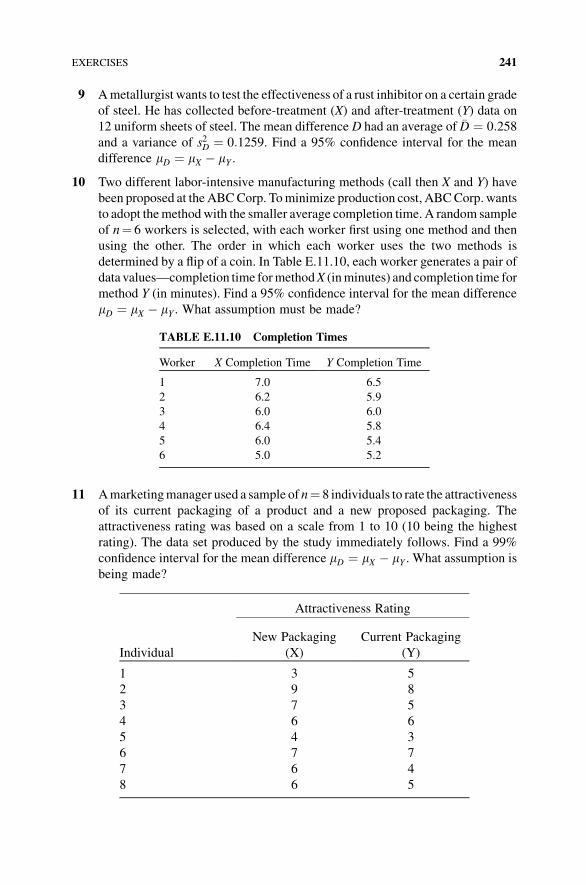
9 Ametallurgist wants to test the effectiveness of a rust inhibitor on a certain grade
of steel. He has collected before-treatment (X) and after-treatment (Y) data on
12 uniform sheets of steel. The mean difference D had an average of �D ¼ 0:258and a variance of s2D ¼ 0:1259. Find a 95% confidence interval for the mean
difference mD ¼ mX � mY .
10 Two different labor-intensive manufacturing methods (call then X and Y) have
been proposed at theABCCorp. Tominimize production cost, ABCCorp. wants
to adopt themethodwith the smaller average completion time. A random sample
of n¼ 6 workers is selected, with each worker first using one method and then
using the other. The order in which each worker uses the two methods is
determined by a flip of a coin. In Table E.11.10, each worker generates a pair of
data values—completion time formethodX (inminutes) and completion time for
method Y (in minutes). Find a 95% confidence interval for the mean difference
mD ¼ mX � mY . What assumption must be made?
11 Amarketingmanager used a sample of n¼ 8 individuals to rate the attractiveness
of its current packaging of a product and a new proposed packaging. The
attractiveness rating was based on a scale from 1 to 10 (10 being the highest
rating). The data set produced by the study immediately follows. Find a 99%
confidence interval for the mean difference mD ¼ mX � mY . What assumption is
being made?
Attractiveness Rating
Individual
New Packaging
(X)
Current Packaging
(Y)
1 3 5
2 9 8
3 7 5
4 6 6
5 4 3
6 7 7
7 6 4
8 6 5
TABLE E.11.10 Completion Times
Worker X Completion Time Y Completion Time
1 7.0 6.5
2 6.2 5.9
3 6.0 6.0
4 6.4 5.8
5 6.0 5.4
6 5.0 5.2
EXERCISES 241
12 Samples of size 200 (¼ nX¼ nY) are taken from each of two independent
binomial populations. They contained X¼ 104 and Y¼ 96 successes, respec-
tively. Find a 95% confidence interval for pX� pY.
13 A sample of 500 people was classified as being health conscious or not. Among
nX¼ 300 individuals classified as health conscious, it was found that X¼ 48
regularly eat yogurt for breakfast. Among the nY¼ 200 persons who were
classified as not health conscious, Y¼ 52 regularly eat yogurt for breakfast.
Find a 99% confidence interval for the difference in the proportions pX� pY of
persons who regularly eat yogurt for breakfast.
14 A random sample containing nX¼ 467males and nY¼ 433 females under the age
of 50 yrs old exhibited X¼ 8 males that were hard of hearing while only Y¼ 1
female possessed this problem. Find a 90% confidence interval for the difference
pX� pY.
15 For Exercise 11.1, testH0 : mX � mY ¼ 0, againstH1 : mX � mYH0 for a¼ 0.05.
What is the p-value?
16 For Exercise 11.2, does mX lie significantly above mY at the a¼ 0.10 level?What
is the test’s p-value?
17 For Exercise 11.3, test H0 : mX � mY ¼ 2000 versus H1 : mX � mY$0 for a¼0.05. What is the p-value?
18 For Exercise 11.4, test H0 : mX � mY ¼ 0 versus H1 : mX � mY$0 for a¼ 0.05.
What is the p-value?
19 For Exercise 11.5, testH0 : mX � mY ¼ 0; againstH1 : mX � mYG0 for a¼ 0.05.
Determine the p-value.
20 For Exercise 11.7, test H0 : mX � mY ¼ 7; against H1 : mX � mYG7 at the 5%
level. Determine the test’s p-value.
21 For Exercise 11.9, test mD ¼ 0 versus H1 : mDH0 for a¼ 0.05. Also, find the
test’s p-value.
22 For Exercise 11.10, test H0 : mD ¼ 0; against H1 : mD$0 for a¼ 0.01. Find the
test’s p-value.
23 For Exercise 11.11, test the hypothesis that the mean attractiveness rating for the
new packaging is at least as good as the mean attractiveness rating for the old
packaging. Use a¼ 0.05. What is the p-value?
24 For Exercise 11.12, testH0 : p1 � p2 ¼ 0 versusH1 : pX � pYH0 at the 5% level
of significance. Determine the p-value.
25 For Exercise 11.13, test H0 : p1 � p2 ¼ 0 versus H1 : pX � pY$0 for a¼ 0.01.
Find the p-value for the test.
26 For Exercise 11.14, test H0 : pX � pY ¼ 0 versus H1 : pX � pY$0 for a¼ 0.05.
What is the p-value?
242 COMPARING TWO POPULATION MEANS AND TWO POPULATION PROPORTIONS
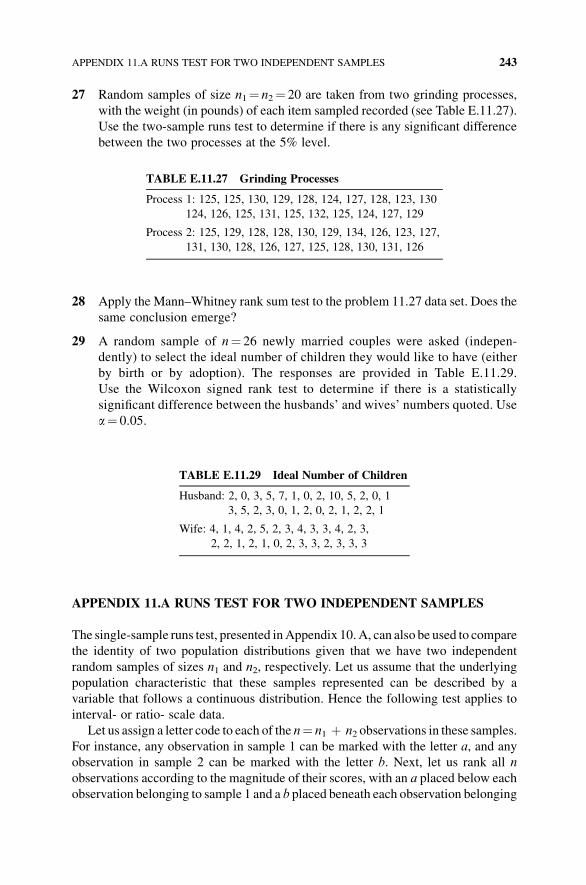
27 Random samples of size n1¼ n2¼ 20 are taken from two grinding processes,
with the weight (in pounds) of each item sampled recorded (see Table E.11.27).
Use the two-sample runs test to determine if there is any significant difference
between the two processes at the 5% level.
28 Apply the Mann–Whitney rank sum test to the problem 11.27 data set. Does the
same conclusion emerge?
29 A random sample of n¼ 26 newly married couples were asked (indepen-
dently) to select the ideal number of children they would like to have (either
by birth or by adoption). The responses are provided in Table E.11.29.
Use the Wilcoxon signed rank test to determine if there is a statistically
significant difference between the husbands’ and wives’ numbers quoted. Use
a¼ 0.05.
APPENDIX 11.A RUNS TEST FOR TWO INDEPENDENT SAMPLES
The single-sample runs test, presented inAppendix 10.A, can also be used to compare
the identity of two population distributions given that we have two independent
random samples of sizes n1 and n2, respectively. Let us assume that the underlying
population characteristic that these samples represented can be described by a
variable that follows a continuous distribution. Hence the following test applies to
interval- or ratio- scale data.
Let us assign a letter code to each of the n¼ n1 þ n2 observations in these samples.
For instance, any observation in sample 1 can be marked with the letter a, and any
observation in sample 2 can be marked with the letter b. Next, let us rank all n
observations according to the magnitude of their scores, with an a placed below each
observation belonging to sample 1 and a b placed beneath each observation belonging
TABLE E.11.27 Grinding Processes
Process 1: 125, 125, 130, 129, 128, 124, 127, 128, 123, 130
124, 126, 125, 131, 125, 132, 125, 124, 127, 129
Process 2: 125, 129, 128, 128, 130, 129, 134, 126, 123, 127,
131, 130, 128, 126, 127, 125, 128, 130, 131, 126
TABLE E.11.29 Ideal Number of Children
Husband: 2, 0, 3, 5, 7, 1, 0, 2, 10, 5, 2, 0, 1
3, 5, 2, 3, 0, 1, 2, 0, 2, 1, 2, 2, 1
Wife: 4, 1, 4, 2, 5, 2, 3, 4, 3, 3, 4, 2, 3,
2, 2, 1, 2, 1, 0, 2, 3, 3, 2, 3, 3, 3
APPENDIX 11.A RUNS TEST FOR TWO INDEPENDENT SAMPLES 243
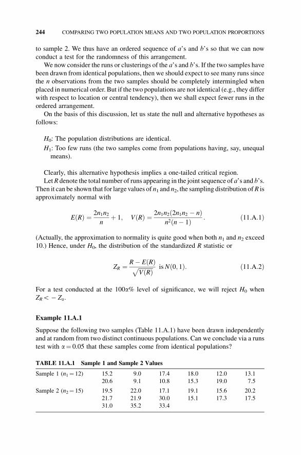
to sample 2. We thus have an ordered sequence of a’s and b’s so that we can now
conduct a test for the randomness of this arrangement.
We now consider the runs or clusterings of the a’s and b’s. If the two samples have
been drawn from identical populations, then we should expect to see many runs since
the n observations from the two samples should be completely intermingled when
placed in numerical order. But if the two populations are not identical (e.g., they differ
with respect to location or central tendency), then we shall expect fewer runs in the
ordered arrangement.
On the basis of this discussion, let us state the null and alternative hypotheses as
follows:
H0: The population distributions are identical.
H1: Too few runs (the two samples come from populations having, say, unequal
means).
Clearly, this alternative hypothesis implies a one-tailed critical region.
LetR denote the total number of runs appearing in the joint sequence of a’s and b’s.
Then it can be shown that for largevalues of n1 and n2, the sampling distribution ofR is
approximately normal with
EðRÞ ¼ 2n1n2
nþ 1; VðRÞ ¼ 2n1n2ð2n1n2 � nÞ
n2 n� 1ð Þ : ð11:A:1Þ
(Actually, the approximation to normality is quite good when both n1 and n2 exceed
10.) Hence, under H0, the distribution of the standardized R statistic or
ZR ¼ R� EðRÞffiffiffiffiffiffiffiffiffiffiVðRÞp isNð0; 1Þ: ð11:A:2Þ
For a test conducted at the 100a% level of significance, we will reject H0 when
ZRG� Za.
Example 11.A.1
Suppose the following two samples (Table 11.A.1) have been drawn independently
and at random from two distinct continuous populations. Can we conclude via a runs
test with a¼ 0.05 that these samples come from identical populations?
TABLE 11.A.1 Sample 1 and Sample 2 Values
Sample 1 (n1¼ 12) 15.2 9.0 17.4 18.0 12.0 13.1
20.6 9.1 10.8 15.3 19.0 7.5
Sample 2 (n2¼ 15) 19.5 22.0 17.1 19.1 15.6 20.2
21.7 21.9 30.0 15.1 17.3 17.5
31.0 35.2 33.4
244 COMPARING TWO POPULATION MEANS AND TWO POPULATION PROPORTIONS
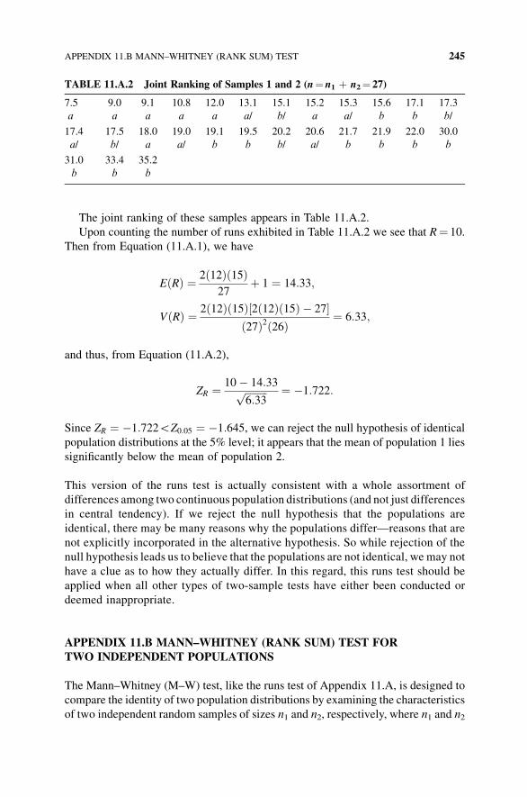
The joint ranking of these samples appears in Table 11.A.2.
Upon counting the number of runs exhibited in Table 11.A.2 we see that R¼ 10.
Then from Equation (11.A.1), we have
EðRÞ ¼ 2ð12Þð15Þ27
þ 1 ¼ 14:33;
VðRÞ ¼ 2ð12Þð15Þ 2ð12Þð15Þ � 27½ �ð27Þ2ð26Þ ¼ 6:33;
and thus, from Equation (11.A.2),
ZR ¼ 10� 14:33ffiffiffiffiffiffiffiffiffi6:33
p ¼ �1:722:
Since ZR ¼ �1:722GZ0:05 ¼ �1:645, we can reject the null hypothesis of identical
population distributions at the 5% level; it appears that the mean of population 1 lies
significantly below the mean of population 2.
This version of the runs test is actually consistent with a whole assortment of
differences among two continuous population distributions (and not just differences
in central tendency). If we reject the null hypothesis that the populations are
identical, there may be many reasons why the populations differ—reasons that are
not explicitly incorporated in the alternative hypothesis. So while rejection of the
null hypothesis leads us to believe that the populations are not identical, we may not
have a clue as to how they actually differ. In this regard, this runs test should be
applied when all other types of two-sample tests have either been conducted or
deemed inappropriate.
APPENDIX 11.B MANN–WHITNEY (RANK SUM) TEST FOR
TWO INDEPENDENT POPULATIONS
The Mann–Whitney (M–W) test, like the runs test of Appendix 11.A, is designed to
compare the identity of two population distributions by examining the characteristics
of two independent random samples of sizes n1 and n2, respectively, where n1 and n2
TABLE 11.A.2 Joint Ranking of Samples 1 and 2 (n¼ n1 þ n2¼ 27)
7.5 9.0 9.1 10.8 12.0 13.1 15.1 15.2 15.3 15.6 17.1 17.3
a a a a a a/ b/ a a/ b b b/
17.4 17.5 18.0 19.0 19.1 19.5 20.2 20.6 21.7 21.9 22.0 30.0
a/ b/ a a/ b b b/ a/ b b b b
31.0 33.4 35.2
b b b
APPENDIX 11.B MANN–WHITNEY (RANK SUM) TEST 245
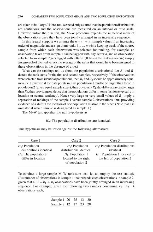
are taken to be “large.”Here, too,weneedonly assume that the populationdistributions
are continuous and the observations are measured on an interval or ratio scale.
However, unlike the runs test, the M–W procedure exploits the numerical ranks of
the observations once they have been jointly arranged in an increasing sequence.
In this regard, suppose we arrange the n¼ n1 þ n2 sample values in an increasing
order of magnitude and assign them ranks 1, . . ., n while keeping track of the sourcesample from which each observation was selected for ranking, for example, an
observation taken from sample 1 can be tagged with, say, letter a, and an observation
selected from sample 2 gets tagged with letter b. (If ties in the rankings occur) simply
assign each of the tied values the average of the ranks thatwould have been assigned to
these observations in the absence of a tie.)
What can the rankings tell us about the population distributions? Let R1 and R2
denote the rank sums for the first and second samples, respectively. If the observations
were selected from identical populations, thenR1 andR2 should be approximately equal
in value. However, if the data points in, say, population 1 tend to be larger than those in
population 2 (given equal sample sizes), then obviouslyR1 should be appreciable larger
thanR2, thus providing evidence that the populations differ in some fashion (typically in
location or central tendency). Hence very large or very small values of R1 imply a
separation of rankings of the sample 1 versus sample 2 observations, thus providing
evidence of a shift in the location of one population relative to the other. (Note that it is
immaterial which sample is designated as sample 1.)
The M–W test specifies the null hypothesis as
H0: The population distributions are identical.
This hypothesis may be tested against the following alternatives:
Case 1 Case 2 Case 3
H0: Population
distributions identical
H0: Population
distributions identical
H0: Population distributions
identical
H1: The populations
differ in location
H1: Population 1
located to the right
of population 2
H1: Population 1 located to
the left of population 2
To conduct a large-sample M–W rank-sum test, let us employ the test statistic
U¼ number of observations in sample 1 that precede each observations in sample 2,
given that all n¼ n1 þ n2 observations have been jointly arranged in an increasing
sequence. For example, given the following two samples containing n1¼ n2¼ 4
observations each,
Sample 1: 20 25 13 30
Sample 2: 12 17 23 28
246 COMPARING TWO POPULATION MEANS AND TWO POPULATION PROPORTIONS
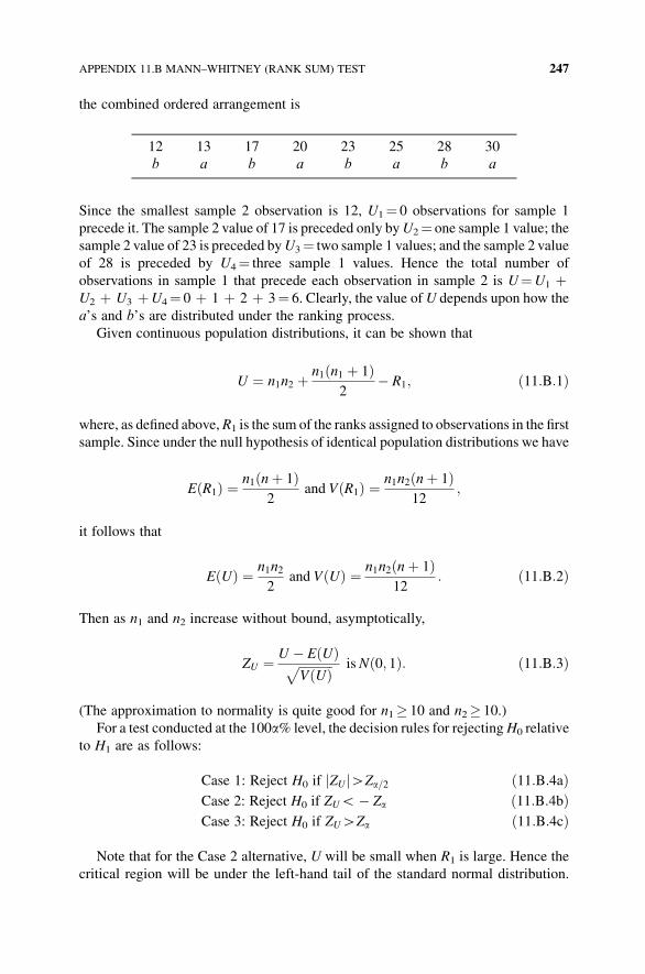
the combined ordered arrangement is
12 13 17 20 23 25 28 30
b a b a b a b a
Since the smallest sample 2 observation is 12, U1¼ 0 observations for sample 1
precede it. The sample 2 value of 17 is preceded only byU2¼ one sample 1 value; the
sample 2 value of 23 is preceded byU3¼ two sample 1 values; and the sample 2 value
of 28 is preceded by U4¼ three sample 1 values. Hence the total number of
observations in sample 1 that precede each observation in sample 2 is U¼U1 þU2 þ U3 þU4¼ 0 þ 1 þ 2 þ 3¼ 6. Clearly, the value of U depends upon how the
a’s and b’s are distributed under the ranking process.
Given continuous population distributions, it can be shown that
U ¼ n1n2 þ n1 n1 þ 1ð Þ2
� R1; ð11:B:1Þ
where, as defined above, R1 is the sum of the ranks assigned to observations in the first
sample. Since under the null hypothesis of identical population distributions we have
EðR1Þ ¼ n1 nþ 1ð Þ2
and VðR1Þ ¼ n1n2 nþ 1ð Þ12
;
it follows that
EðUÞ ¼ n1n2
2and VðUÞ ¼ n1n2 nþ 1ð Þ
12: ð11:B:2Þ
Then as n1 and n2 increase without bound, asymptotically,
ZU ¼ U � EðUÞffiffiffiffiffiffiffiffiffiffiffiVðUÞp is Nð0; 1Þ: ð11:B:3Þ
(The approximation to normality is quite good for n1� 10 and n2� 10.)
For a test conducted at the 100a% level, the decision rules for rejectingH0 relative
to H1 are as follows:
Case 1: Reject H0 if ZUj jHZa=2 ð11:B:4aÞCase 2: Reject H0 if ZUG� Za ð11:B:4bÞCase 3: Reject H0 if ZUHZa ð11:B:4cÞ
Note that for the Case 2 alternative, U will be small when R1 is large. Hence the
critical region will be under the left-hand tail of the standard normal distribution.
APPENDIX 11.B MANN–WHITNEY (RANK SUM) TEST 247
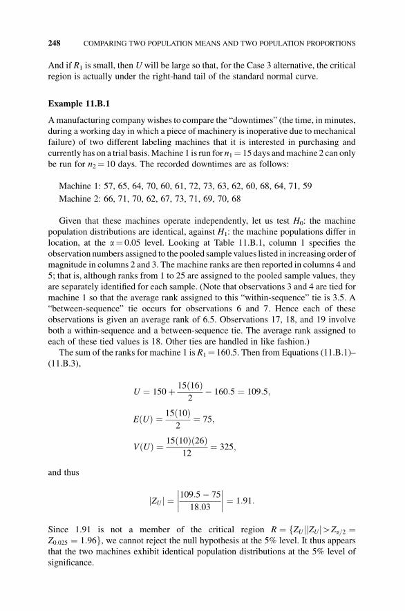
And if R1 is small, then U will be large so that, for the Case 3 alternative, the critical
region is actually under the right-hand tail of the standard normal curve.
Example 11.B.1
Amanufacturing company wishes to compare the “downtimes” (the time, in minutes,
during a working day in which a piece of machinery is inoperative due to mechanical
failure) of two different labeling machines that it is interested in purchasing and
currently has on a trial basis.Machine 1 is run for n1¼ 15 days andmachine 2 can only
be run for n2¼ 10 days. The recorded downtimes are as follows:
Machine 1: 57, 65, 64, 70, 60, 61, 72, 73, 63, 62, 60, 68, 64, 71, 59
Machine 2: 66, 71, 70, 62, 67, 73, 71, 69, 70, 68
Given that these machines operate independently, let us test H0: the machine
population distributions are identical, against H1: the machine populations differ in
location, at the a¼ 0.05 level. Looking at Table 11.B.1, column 1 specifies the
observation numbers assigned to the pooled sample values listed in increasing order of
magnitude in columns 2 and 3. The machine ranks are then reported in columns 4 and
5; that is, although ranks from 1 to 25 are assigned to the pooled sample values, they
are separately identified for each sample. (Note that observations 3 and 4 are tied for
machine 1 so that the average rank assigned to this “within-sequence” tie is 3.5. A
“between-sequence” tie occurs for observations 6 and 7. Hence each of these
observations is given an average rank of 6.5. Observations 17, 18, and 19 involve
both a within-sequence and a between-sequence tie. The average rank assigned to
each of these tied values is 18. Other ties are handled in like fashion.)
The sum of the ranks for machine 1 is R1¼ 160.5. Then from Equations (11.B.1)–
(11.B.3),
U ¼ 150þ 15ð16Þ2
� 160:5 ¼ 109:5;
EðUÞ ¼ 15ð10Þ2
¼ 75;
VðUÞ ¼ 15ð10Þð26Þ12
¼ 325;
and thus
ZUj j ¼ 109:5� 75
18:03
¼ 1:91:
Since 1.91 is not a member of the critical region R ¼ ZUf j ZUj jHZa=2 ¼Z0:025 ¼ 1:96g, we cannot reject the null hypothesis at the 5% level. It thus appears
that the two machines exhibit identical population distributions at the 5% level of
significance.
248 COMPARING TWO POPULATION MEANS AND TWO POPULATION PROPORTIONS
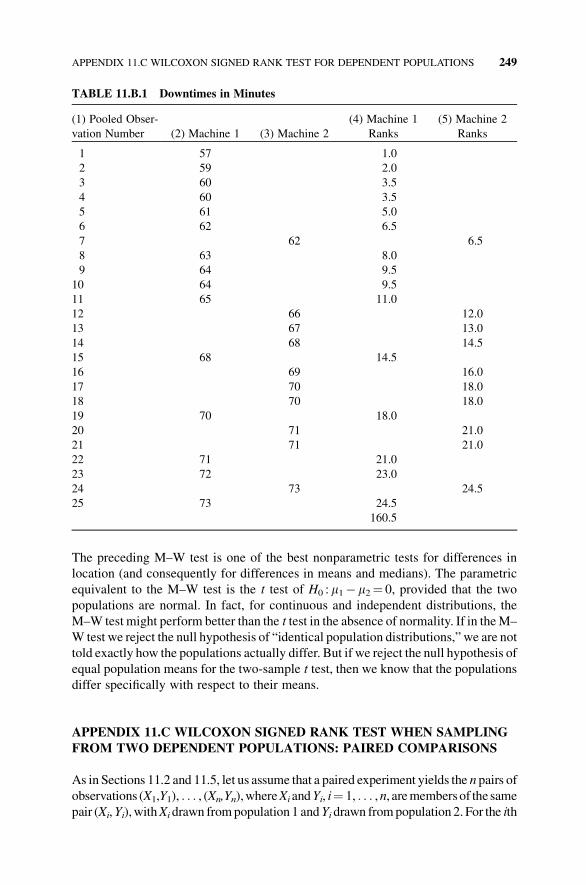
The preceding M–W test is one of the best nonparametric tests for differences in
location (and consequently for differences in means and medians). The parametric
equivalent to the M–W test is the t test of H0 :m1� m2¼ 0, provided that the two
populations are normal. In fact, for continuous and independent distributions, the
M–W test might perform better than the t test in the absence of normality. If in theM–
W test we reject the null hypothesis of “identical population distributions,” we are not
told exactly how the populations actually differ. But if we reject the null hypothesis of
equal population means for the two-sample t test, then we know that the populations
differ specifically with respect to their means.
APPENDIX 11.C WILCOXON SIGNED RANK TEST WHEN SAMPLING
FROM TWO DEPENDENT POPULATIONS: PAIRED COMPARISONS
As in Sections 11.2 and 11.5, let us assume that a paired experiment yields the n pairs of
observations (X1,Y1), . . . , (Xn,Yn),whereXi andYi, i¼ 1, . . . ,n, aremembersof the same
pair (Xi,Yi),withXi drawn frompopulation 1 andYi drawn frompopulation 2. For the ith
TABLE 11.B.1 Downtimes in Minutes
(1) Pooled Obser-
vation Number (2) Machine 1 (3) Machine 2
(4) Machine 1
Ranks
(5) Machine 2
Ranks
1 57 1.0
2 59 2.0
3 60 3.5
4 60 3.5
5 61 5.0
6 62 6.5
7 62 6.5
8 63 8.0
9 64 9.5
10 64 9.5
11 65 11.0
12 66 12.0
13 67 13.0
14 68 14.5
15 68 14.5
16 69 16.0
17 70 18.0
18 70 18.0
19 70 18.0
20 71 21.0
21 71 21.0
22 71 21.0
23 72 23.0
24 73 24.5
25 73 24.5
160.5
APPENDIX 11.C WILCOXON SIGNED RANK TEST FOR DEPENDENT POPULATIONS 249
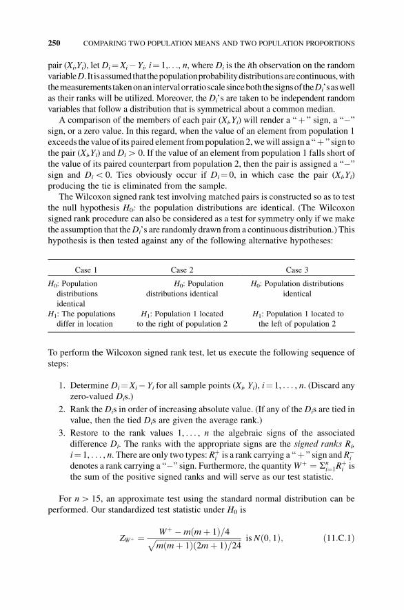
pair (Xi,Yi), let Di¼Xi� Yi, i¼ 1,. . ., n, where Di is the ith observation on the random
variableD. It isassumedthatthepopulationprobabilitydistributionsarecontinuous,with
themeasurements takenonanintervalorratioscalesinceboth thesignsof theDi’saswell
as their ranks will be utilized. Moreover, the Di’s are taken to be independent random
variables that follow a distribution that is symmetrical about a common median.
A comparison of the members of each pair (Xi,Yi) will render a “þ ” sign, a “�”
sign, or a zero value. In this regard, when the value of an element from population 1
exceeds thevalue of its paired element frompopulation 2,wewill assign a “þ ” sign to
the pair (Xi,Yi) and DiH 0. If the value of an element from population 1 falls short of
the value of its paired counterpart from population 2, then the pair is assigned a “�”
sign and DiG 0. Ties obviously occur if Di¼ 0, in which case the pair (Xi,Yi)
producing the tie is eliminated from the sample.
TheWilcoxon signed rank test involving matched pairs is constructed so as to test
the null hypothesis H0: the population distributions are identical. (The Wilcoxon
signed rank procedure can also be considered as a test for symmetry only if we make
the assumption that theDi’s are randomly drawn from a continuous distribution.) This
hypothesis is then tested against any of the following alternative hypotheses:
Case 1 Case 2 Case 3
H0: Population
distributions
identical
H0: Population
distributions identical
H0: Population distributions
identical
H1: The populations
differ in location
H1: Population 1 located
to the right of population 2
H1: Population 1 located to
the left of population 2
To perform the Wilcoxon signed rank test, let us execute the following sequence of
steps:
1. Determine Di¼Xi� Yi for all sample points (Xi, Yi), i¼ 1, . . . , n. (Discard anyzero-valued Dis.)
2. Rank the Dis in order of increasing absolute value. (If any of the Dis are tied in
value, then the tied Dis are given the average rank.)
3. Restore to the rank values 1, . . . , n the algebraic signs of the associated
difference Di. The ranks with the appropriate signs are the signed ranks Ri,
i¼ 1, . . . , n. There are only two types: Rþi is a rank carrying a “þ ” sign and R�
i
denotes a rank carrying a “�” sign. Furthermore, the quantityWþ ¼ Sni¼1R
þi is
the sum of the positive signed ranks and will serve as our test statistic.
For nH 15, an approximate test using the standard normal distribution can be
performed. Our standardized test statistic under H0 is
ZWþ ¼ Wþ �mðmþ 1Þ=4ffiffiffiffiffiffiffiffiffiffiffiffiffiffiffiffiffiffiffiffiffiffiffiffiffiffiffiffiffiffiffiffiffiffiffiffiffiffiffiffiffiffiffiffiffimðmþ 1Þð2mþ 1Þ=24p is Nð0; 1Þ; ð11:C:1Þ
250 COMPARING TWO POPULATION MEANS AND TWO POPULATION PROPORTIONS
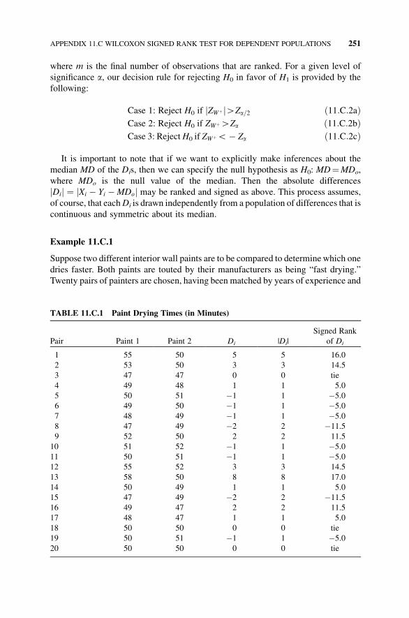
where m is the final number of observations that are ranked. For a given level of
significance a, our decision rule for rejecting H0 in favor of H1 is provided by the
following:
Case 1: Reject H0 if ZWþj jHZa=2 ð11:C:2aÞCase 2: Reject H0 if ZWþHZa ð11:C:2bÞCase 3: RejectH0 if ZWþG� Za ð11:C:2cÞ
It is important to note that if we want to explicitly make inferences about the
median MD of the Dis, then we can specify the null hypothesis as H0: MD¼MDo,
where MDo is the null value of the median. Then the absolute differences
Dij j ¼ Xi � Yi �MDoj j may be ranked and signed as above. This process assumes,
of course, that eachDi is drawn independently from a population of differences that is
continuous and symmetric about its median.
Example 11.C.1
Suppose two different interior wall paints are to be compared to determine which one
dries faster. Both paints are touted by their manufacturers as being “fast drying.”
Twenty pairs of painters are chosen, having been matched by years of experience and
TABLE 11.C.1 Paint Drying Times (in Minutes)
Pair Paint 1 Paint 2 Di |Di|
Signed Rank
of Di
1 55 50 5 5 16.0
2 53 50 3 3 14.5
3 47 47 0 0 tie
4 49 48 1 1 5.0
5 50 51 �1 1 �5.0
6 49 50 �1 1 �5.0
7 48 49 �1 1 �5.0
8 47 49 �2 2 �11.5
9 52 50 2 2 11.5
10 51 52 �1 1 �5.0
11 50 51 �1 1 �5.0
12 55 52 3 3 14.5
13 58 50 8 8 17.0
14 50 49 1 1 5.0
15 47 49 �2 2 �11.5
16 49 47 2 2 11.5
17 48 47 1 1 5.0
18 50 50 0 0 tie
19 50 51 �1 1 �5.0
20 50 50 0 0 tie
APPENDIX 11.C WILCOXON SIGNED RANK TEST FOR DEPENDENT POPULATIONS 251
skill level. The times to drying (in minutes) of walls of similar sizes and textures are
presented in Table 11.C.1. For a¼ 0.05, determine if the underlying distributions of
drying times differ significantly in terms of time to drying. Clearly, Case 1 applies.
Given three ties, n is reduced to m¼ 17, with Wþ ¼ 95, and thus, via Equa-
tion (11.C.1),
ZWþ ¼ 95� 17ð18Þ=4ffiffiffiffiffiffiffiffiffiffiffiffiffiffiffiffiffiffiffiffiffiffiffiffiffiffiffiffiffiffi17ð18Þð35Þ=24p ¼ 0:88:
Since 0.88 does not fall within the critical regionR ¼ ZWþf j ZWþj jH1:96g, we cannotreject the null hypothesis; at the 5% level of significance, the two drying time
population distributions are essentially identical.
The preceding Wilcoxon signed rank test is the test of choice among nonparametric
tests that hypothesize identical population distributions under paired comparisons.
Given a sample ofmatched pairs, the test is useful in determiningwhether themedians
of the population distributions are identical, or whether one such distribution is
located to the right or left of the other. In the instance where the assumption of
normality cannot be justified, the nonparametric Wilcoxon signed rank test should be
utilized instead of the parametric t test for matched pairs since the latter test explicitly
assumes normality.
252 COMPARING TWO POPULATION MEANS AND TWO POPULATION PROPORTIONS
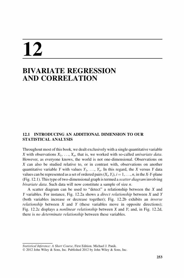
12BIVARIATE REGRESSIONAND CORRELATION
12.1 INTRODUCING AN ADDITIONAL DIMENSION TO OUR
STATISTICAL ANALYSIS
Throughout most of this book, we dealt exclusively with a single quantitative variable
X with observations X1, . . ., Xn, that is, we worked with so-called univariate data.
However, as everyone knows, the world is not one-dimensional. Observations on
X can also be studied relative to, or in contrast with, observations on another
quantitative variable Y with values Y1, . . ., Yn. In this regard, the X versus Y data
values can be represented as a set of ordered pairs (Xi,Yi), i¼ 1, . . ., n, in theX-Y-plane(Fig. 12.1). This type of two-dimensional graph is termed a scatter diagram involving
bivariate data. Such data will now constitute a sample of size n.
A scatter diagram can be used to “detect” a relationship between the X and
Y variables. For instance, Fig. 12.2a shows a direct relationship between X and Y
(both variables increase or decrease together); Fig. 12.2b exhibits an inverse
relationship between X and Y (these variables move in opposite directions);
Fig. 12.2c displays a nonlinear relationship between X and Y; and, in Fig. 12.2d,
there is no determinate relationship between these variables.
Statistical Inference: A Short Course, First Edition. Michael J. Panik.� 2012 John Wiley & Sons, Inc. Published 2012 by John Wiley & Sons, Inc.
253
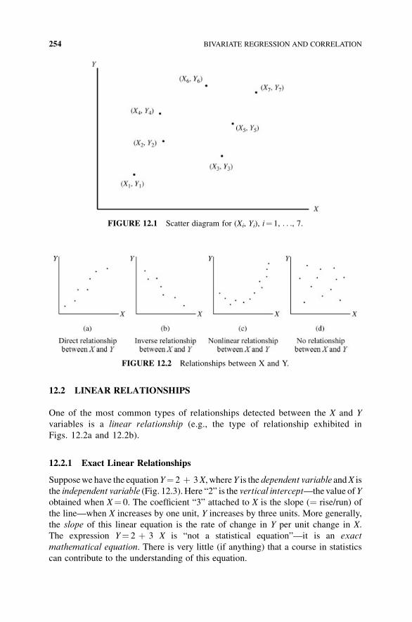
12.2 LINEAR RELATIONSHIPS
One of the most common types of relationships detected between the X and Y
variables is a linear relationship (e.g., the type of relationship exhibited in
Figs. 12.2a and 12.2b).
12.2.1 Exact Linear Relationships
Supposewe have the equationY¼ 2 þ 3X, where Y is the dependent variable andX is
the independent variable (Fig. 12.3). Here “2” is the vertical intercept—thevalue of Y
obtained when X¼ 0. The coefficient “3” attached to X is the slope (¼ rise/run) of
the line—when X increases by one unit, Y increases by three units. More generally,
the slope of this linear equation is the rate of change in Y per unit change in X.
The expression Y¼ 2 þ 3 X is “not a statistical equation”—it is an exact
mathematical equation. There is very little (if anything) that a course in statistics
can contribute to the understanding of this equation.
FIGURE 12.2 Relationships between X and Y.
FIGURE 12.1 Scatter diagram for (Xi, Yi), i¼ 1, . . ., 7.
254 BIVARIATE REGRESSION AND CORRELATION
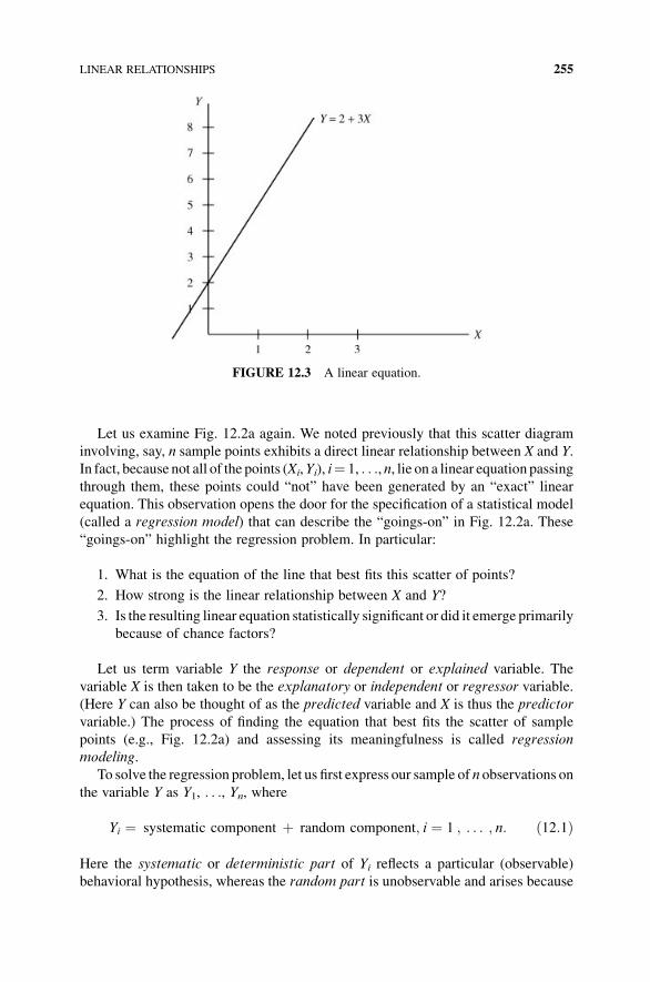
Let us examine Fig. 12.2a again. We noted previously that this scatter diagram
involving, say, n sample points exhibits a direct linear relationship between X and Y.
In fact, because not all of the points (Xi,Yi), i¼ 1, . . .,n, lie on a linear equation passingthrough them, these points could “not” have been generated by an “exact” linear
equation. This observation opens the door for the specification of a statistical model
(called a regression model) that can describe the “goings-on” in Fig. 12.2a. These
“goings-on” highlight the regression problem. In particular:
1. What is the equation of the line that best fits this scatter of points?
2. How strong is the linear relationship between X and Y?
3. Is the resulting linear equation statistically significant or did it emerge primarily
because of chance factors?
Let us term variable Y the response or dependent or explained variable. The
variable X is then taken to be the explanatory or independent or regressor variable.
(Here Y can also be thought of as the predicted variable and X is thus the predictor
variable.) The process of finding the equation that best fits the scatter of sample
points (e.g., Fig. 12.2a) and assessing its meaningfulness is called regression
modeling.
To solve the regression problem, let us first express our sample of n observations on
the variable Y as Y1, . . ., Yn, where
Yi ¼ systematic component þ random component; i ¼ 1 ; . . . ; n: ð12:1Þ
Here the systematic or deterministic part of Yi reflects a particular (observable)
behavioral hypothesis, whereas the random part is unobservable and arises because
FIGURE 12.3 A linear equation.
LINEAR RELATIONSHIPS 255
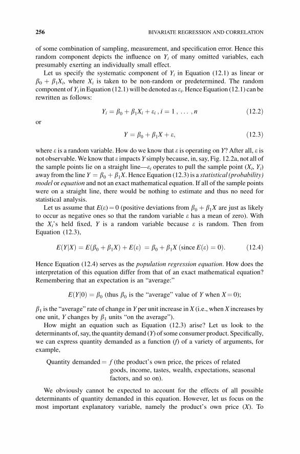
of some combination of sampling, measurement, and specification error. Hence this
random component depicts the influence on Yi of many omitted variables, each
presumably exerting an individually small effect.
Let us specify the systematic component of Yi in Equation (12.1) as linear or
b0 þ b1Xi, where Xi is taken to be non-random or predetermined. The random
component ofYi in Equation (12.1)will be denoted as ei. Hence Equation (12.1) can berewritten as follows:
Yi ¼ b0 þ b1Xi þ ei ; i ¼ 1 ; . . . ; n ð12:2Þor
Y ¼ b0 þ b1X þ e; ð12:3Þ
where e is a random variable. How do we know that e is operating on Y? After all, e isnot observable.We know that e impacts Y simply because, in, say, Fig. 12.2a, not all of
the sample points lie on a straight line—ei operates to pull the sample point (Xi, Yi)
away from the line Y ¼ b0 þ b1X. Hence Equation (12.3) is a statistical (probability)model or equation and not an exact mathematical equation. If all of the sample points
were on a straight line, there would be nothing to estimate and thus no need for
statistical analysis.
Let us assume that E(e)¼ 0 (positive deviations from b0 þ b1X are just as likely
to occur as negative ones so that the random variable e has a mean of zero). With
the Xi’s held fixed, Y is a random variable because e is random. Then from
Equation (12.3),
E Y Xj Þ ¼ E b0 þ b1Xð Þ þ E eð Þ ¼ b0 þ b1X since E eð Þ ¼ 0ð Þ:ð ð12:4Þ
Hence Equation (12.4) serves as the population regression equation. How does the
interpretation of this equation differ from that of an exact mathematical equation?
Remembering that an expectation is an “average:”
EðY 0Þ ¼ b0j (thus b0 is the “average” value of Y when X¼ 0);
b1 is the “average” rate of change in Y per unit increase in X (i.e., when X increases by
one unit, Y changes by b1 units “on the average”).
How might an equation such as Equation (12.3) arise? Let us look to the
determinants of, say, the quantity demand (Y) of some consumer product. Specifically,
we can express quantity demanded as a function (f) of a variety of arguments, for
example,
Quantity demanded¼ f (the product’s own price, the prices of related
goods, income, tastes, wealth, expectations, seasonal
factors, and so on).
We obviously cannot be expected to account for the effects of all possible
determinants of quantity demanded in this equation. However, let us focus on the
most important explanatory variable, namely the product’s own price (X). To
256 BIVARIATE REGRESSION AND CORRELATION
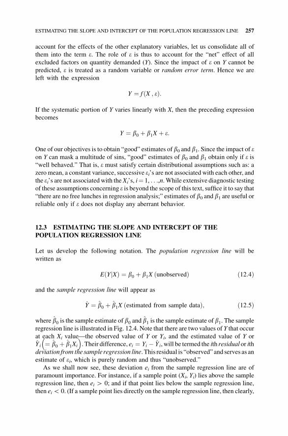
account for the effects of the other explanatory variables, let us consolidate all of
them into the term e. The role of e is thus to account for the “net” effect of all
excluded factors on quantity demanded (Y). Since the impact of e on Y cannot be
predicted, e is treated as a random variable or random error term. Hence we are
left with the expression
Y ¼ f X ; eð Þ:
If the systematic portion of Y varies linearly with X, then the preceding expression
becomes
Y ¼ b0 þ b1X þ e:
One of our objectives is to obtain “good” estimates of b0 and b1. Since the impact of eon Y can mask a multitude of sins, “good” estimates of b0 and b1 obtain only if e is“well behaved.” That is, e must satisfy certain distributional assumptions such as: a
zero mean, a constant variance, successive ei’s are not associated with each other, andthe ei’s are not associated with theXi’s, i¼ 1, . . .,n.While extensive diagnostic testing
of these assumptions concerning e is beyond the scope of this text, suffice it to say that“there are no free lunches in regression analysis;” estimates of b0 and b1 are useful orreliable only if e does not display any aberrant behavior.
12.3 ESTIMATING THE SLOPE AND INTERCEPT OF THE
POPULATION REGRESSION LINE
Let us develop the following notation. The population regression line will be
written as
E Y Xj Þ ¼ b0 þ b1X unobservedð Þð ð12:4Þ
and the sample regression line will appear as
Y ¼ b0 þ b1X estimated from sample datað Þ; ð12:5Þ
where b0 is the sample estimate of b0 and b1 is the sample estimate of b1. The sample
regression line is illustrated in Fig. 12.4. Note that there are two values of Y that occur
at each Xi value—the observed value of Y or Yi, and the estimated value of Y or
Y i ¼ b0 þ b1Xi
� �. Their difference, ei ¼ Yi � Y i, will be termed the ith residual or ith
deviation from the sample regression line. This residual is “observed” and serves as an
estimate of ei, which is purely random and thus “unobserved.”
As we shall now see, these deviation ei from the sample regression line are of
paramount importance. For instance, if a sample point (Xi, Yi) lies above the sample
regression line, then ei H 0; and if that point lies below the sample regression line,
then eiG 0. (If a sample point lies directly on the sample regression line, then clearly,
ESTIMATING THE SLOPE AND INTERCEPT OF THE POPULATION REGRESSION LINE 257
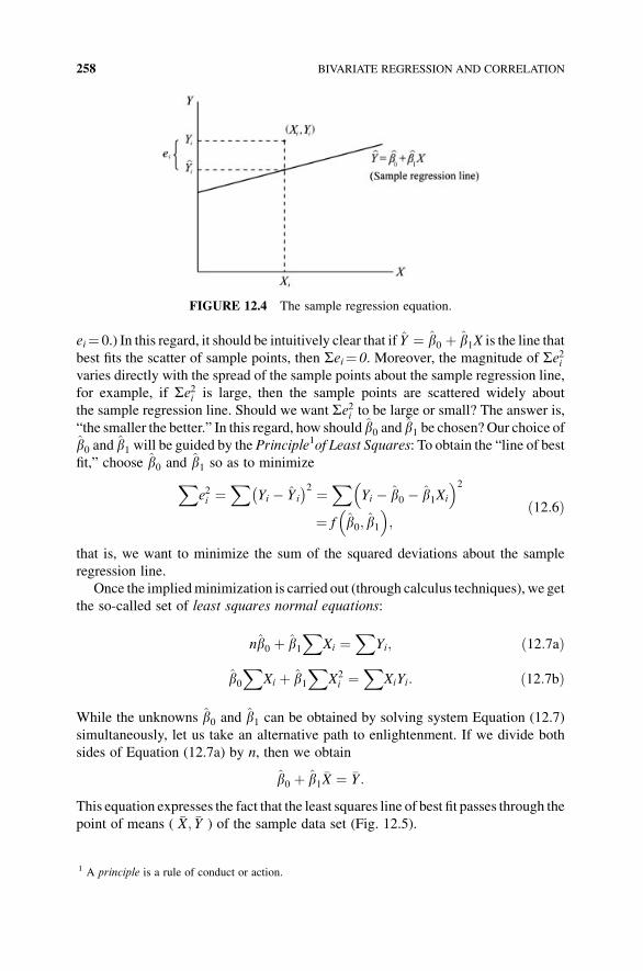
ei¼ 0.) In this regard, it should be intuitively clear that if Y ¼ b0 þ b1X is the line that
best fits the scatter of sample points, then Sei¼ 0. Moreover, the magnitude of Se2ivaries directly with the spread of the sample points about the sample regression line,
for example, if Se2i is large, then the sample points are scattered widely about
the sample regression line. Should we want Se2i to be large or small? The answer is,
“the smaller the better.” In this regard, how should b0 and b1 be chosen?Our choice ofb0 and b1 will be guided by the Principle
1of Least Squares: To obtain the “line of best
fit,” choose b0 and b1 so as to minimize
Xe2i ¼
XYi � Y i
� �2 ¼X
Yi � b0 � b1Xi
� �2
¼ f b0; b1� �
;ð12:6Þ
that is, we want to minimize the sum of the squared deviations about the sample
regression line.
Once the impliedminimization is carried out (through calculus techniques), we get
the so-called set of least squares normal equations:
nb0 þ b1X
Xi ¼X
Yi; ð12:7aÞ
b0X
Xi þ b1X
X2i ¼
XXiYi: ð12:7bÞ
While the unknowns b0 and b1 can be obtained by solving system Equation (12.7)
simultaneously, let us take an alternative path to enlightenment. If we divide both
sides of Equation (12.7a) by n, then we obtain
b0 þ b1�X ¼ �Y :
This equation expresses the fact that the least squares line of best fit passes through the
point of means ( �X; �Y ) of the sample data set (Fig. 12.5).
FIGURE 12.4 The sample regression equation.
1 A principle is a rule of conduct or action.
258 BIVARIATE REGRESSION AND CORRELATION
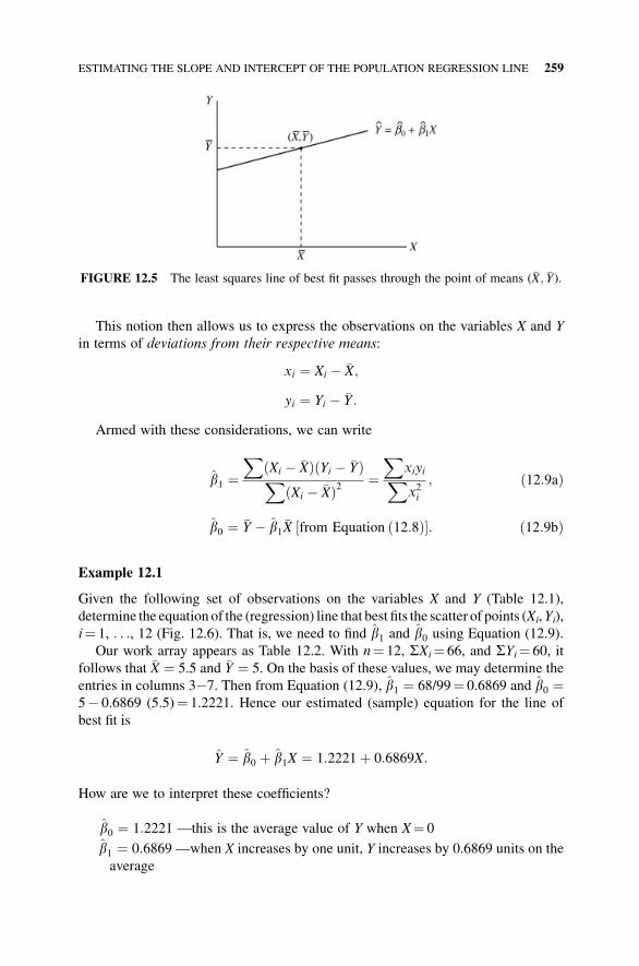
This notion then allows us to express the observations on the variables X and Y
in terms of deviations from their respective means:
xi ¼ Xi � �X;
yi ¼ Yi � �Y :
Armed with these considerations, we can write
b1 ¼X
Xi � �Xð Þ Yi � �Yð ÞX
Xi � �Xð Þ2¼X
xiyiXx2i
; ð12:9aÞ
b0 ¼ �Y � b1�X from Equation 12:8ð Þ½ �: ð12:9bÞ
Example 12.1
Given the following set of observations on the variables X and Y (Table 12.1),
determine the equation of the (regression) line that best fits the scatter of points (Xi,Yi),
i¼ 1, . . ., 12 (Fig. 12.6). That is, we need to find b1 and b0 using Equation (12.9).
Our work array appears as Table 12.2. With n¼ 12, SXi¼ 66, and SYi¼ 60, it
follows that �X ¼ 5.5 and �Y ¼ 5. On the basis of these values, we may determine the
entries in columns 3�7. Then from Equation (12.9), b1 ¼ 68/99¼ 0.6869 and b0 ¼5� 0.6869 (5.5)¼ 1.2221. Hence our estimated (sample) equation for the line of
best fit is
Y ¼ b0 þ b1X ¼ 1:2221þ 0:6869X:
How are we to interpret these coefficients?
b0 ¼ 1:2221 —this is the average value of Y when X¼ 0
b1 ¼ 0:6869 —when X increases by one unit, Y increases by 0.6869 units on the
average
FIGURE 12.5 The least squares line of best fit passes through the point of means (�X; �Y).
ESTIMATING THE SLOPE AND INTERCEPT OF THE POPULATION REGRESSION LINE 259
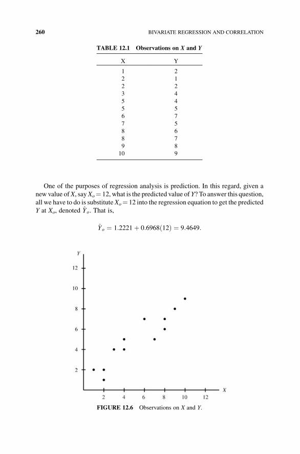
One of the purposes of regression analysis is prediction. In this regard, given a
new value ofX, sayXo¼ 12, what is the predicted value of Y? To answer this question,
all we have to do is substitute Xo¼ 12 into the regression equation to get the predicted
Y at Xo, denoted Yo. That is,
Yo ¼ 1:2221þ 0:6968ð12Þ ¼ 9:4649:
TABLE 12.1 Observations on X and Y
X Y
1 2
2 1
2 2
3 4
5 4
5 5
6 7
7 5
8 6
8 7
9 8
10 9
FIGURE 12.6 Observations on X and Y.
260 BIVARIATE REGRESSION AND CORRELATION
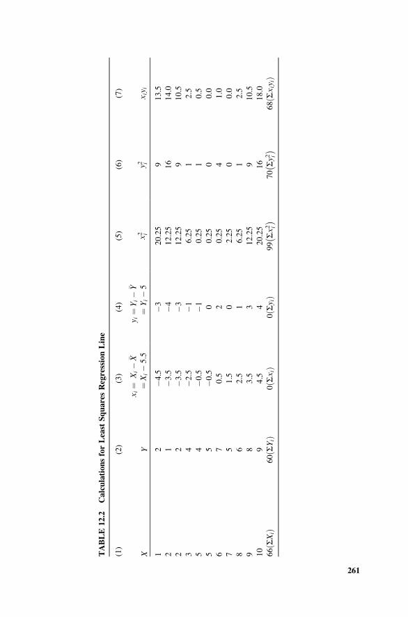
TABLE12.2
CalculationsforLeast
SquaresRegressionLine
(1)
(2)
(3)
(4)
(5)
(6)
(7)
XY
xi¼
Xi�
� X¼Xi�5:5
y i¼Yi�
� Y¼
Yi�5
x2 i
y2 ixiy
i
12
�4.5
�320.25
913.5
21
�3.5
�412.25
16
14.0
22
�3.5
�312.25
910.5
34
�2.5
�16.25
12.5
54
�0.5
�10.25
10.5
55
�0.5
00.25
00.0
67
0.5
20.25
41.0
75
1.5
02.25
00.0
86
2.5
16.25
12.5
98
3.5
312.25
910.5
10
94.5
420.25
16
18.0
66SXi
ðÞ
60SYi
ðÞ
0Sxi
ðÞ
0Sy i
ðÞ
99Sx2 i
��
70Sy2 i
��
68Sxiy
ið
Þ
261
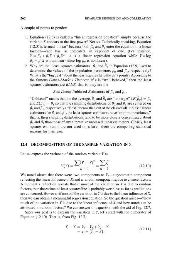
A couple of points to ponder:
1. Equation (12.3) is called a “linear regression equation” simply because the
variable X appears to the first power? Not so. Technically speaking, Equation
(12.3) is termed “linear” because both b0 and b1 enter the equation in a linear
fashion—each has, as indicated, an exponent of one. (For instance,
Y ¼ b0 þ b1X þ b2X2 þ e is a linear regression equation while Y¼ log
b0 þ b1X is nonlinear (since log b0 is nonlinear).2. Why are the “least squares estimators” b0 and b1 in Equation (12.9) used to
determine the values of the population parameters b0 and b1, respectively?What’s the “big deal” about the least squares fit to the data points? According to
the famous Gauss–Markov Theorem, if e is “well behaved,” then the least
squares estimators are BLUE, that is, they are the
Best Linear Unbiased Estimators of b0 and b1:
“Unbiased” means that, on the average, b0 and b1 are “on target” ( Eðb0Þ ¼ b0and Eðb1Þ ¼ b1 so that the sampling distributions of b0 and b1 are centered onb0 andb1, respectively). “Best”means that, out of the class of all unbiased linear
estimators forb0 andb1, the least squares estimators have “minimumvariance,”
that is, their sampling distributions tend to be more closely concentrated about
b0 and b1 than those of any alternative unbiased linear estimators. Clearly, least
squares estimators are not used on a lark—there are compelling statistical
reasons for their use.
12.4 DECOMPOSITION OF THE SAMPLE VARIATION IN Y
Let us express the variance of the random variable Y as
VðYÞ ¼X
ðYi � �YÞ2n� 1
¼X
y2i
n� 1: ð12:10Þ
We noted above that there were two components to Yi—a systematic component
reflecting the linear influence of Xi and a random component ei due to chance factors.A moment’s reflection reveals that if most of the variation in Y is due to random
factors, then the estimated least squares line is probablyworthless as far as predictions
are concerned. However, if most of the variation in Y is due to the linear influence ofX,
then we can obtain a meaningful regression equation. So the question arises—“How
much of the variation in Y is due to the linear influence of X and how much can be
attributed to random factors? We can answer this question with the aid of Fig. 12.7.
Since our goal is to explain the variation in Y, let’s start with the numerator of
Equation (12.10). That is, from Fig. 12.7,
Yi � �Y ¼ Yi � Y i þ Y i � �Y¼ ei þ Y i � �Y
� �;
ð12:11Þ
262 BIVARIATE REGRESSION AND CORRELATION
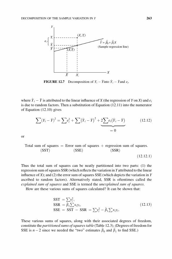
where Y i � �Y is attributed to the linear influence of X (the regression of Y on X) and eiis due to random factors. Then a substitution of Equation (12.11) into the numerator
of Equation (12.10) gives
XYi � �Yð Þ2 ¼
Xe2i þ
XY i � �Y� �2 þ 2
Xei Y i � �Y� �
|fflfflfflfflfflfflfflfflfflfflffl{zfflfflfflfflfflfflfflfflfflfflffl}¼ 0
ð12:12Þ
or
Total sum of squares ¼ Error sum of squares þ regression sum of squares:SSTð Þ SSEð Þ SSRð Þ
ð12:12:1Þ
Thus the total sum of squares can be neatly partitioned into two parts: (1) the
regression sumof squares SSR (which reflects the variation inY attributed to the linear
influence of X); and (2) the error sum of squares SSE (which depicts the variation in Y
ascribed to random factors). Alternatively stated, SSR is oftentimes called the
explained sum of squares and SSE is termed the unexplained sum of squares.
How are these various sums of squares calculated? It can be shown that:
SST ¼Py2i ;
SSR ¼ b1P
xiyi;
SSE ¼ SST � SSR ¼Py2i � b1P
xiyi:
ð12:13Þ
These various sums of squares, along with their associated degrees of freedom,
constitute the partitioned sums of squares table (Table 12.3). (Degrees of freedom for
SSE is n� 2 since we needed the “two” estimates b0 and b1 to find SSE.)
FIGURE 12.7 Decomposition of Yi � �Yinto Y i � �Yand ei.
DECOMPOSITION OF THE SAMPLE VARIATION IN Y 263
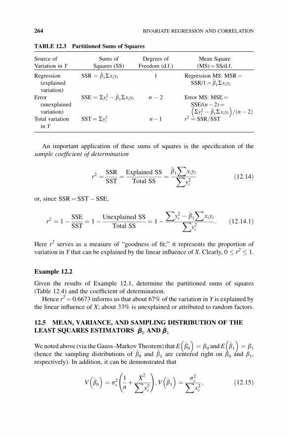
An important application of these sums of squares is the specification of the
sample coefficient of determination
r2 ¼ SSR
SST¼ Explained SS
Total SS¼ b1
XxiyiXy2i
ð12:14Þ
or, since SSR¼ SST� SSE,
r2 ¼ 1� SSE
SST¼ 1� Unexplained SS
Total SS¼ 1�
Xy2i � b1
XxiyiX
y2i: ð12:14:1Þ
Here r2 serves as a measure of “goodness of fit;” it represents the proportion of
variation in Y that can be explained by the linear influence of X. Clearly, 0 � r2 � 1.
Example 12.2
Given the results of Example 12.1, determine the partitioned sums of squares
(Table 12.4) and the coefficient of determination.
Hence r2¼ 0.6673 informs us that about 67% of the variation in Y is explained by
the linear influence of X; about 33% is unexplained or attributed to random factors.
12.5 MEAN, VARIANCE, AND SAMPLING DISTRIBUTION OF THE
LEAST SQUARES ESTIMATORS b0 AND b1
We noted above (via theGauss–Markov Theorem) thatE b0� �
¼ b0 andE b1� �
¼ b1(hence the sampling distributions of b0 and b1 are centered right on b0 and b1,respectively). In addition, it can be demonstrated that
V b0� �
¼ s2e1
nþ
�X2
Xx2i
!;V b1� �
¼ s2eXx2i
; ð12:15Þ
TABLE 12.3 Partitioned Sums of Squares
Source of
Variation in Y
Sums of
Squares (SS)
Degrees of
Freedom (d.f.)
Mean Square
(MS)¼ SS/d.f.
Regression
(explained
variation)
SSR ¼ b1Sxiyi 1 Regression MS: MSR¼SSR/1¼ b1Sxiyi
Error
(unexplained
variation)
SSE ¼ Sy2i � b1Sxiyi n � 2 Error MS: MSE¼SSE/(n� 2)¼Sy2i � b1Sxiyi� �
= n� 2ð ÞTotal variation
in Y
SST¼ Sy2i n� 1 r2 ¼ SSR=SST
264 BIVARIATE REGRESSION AND CORRELATION
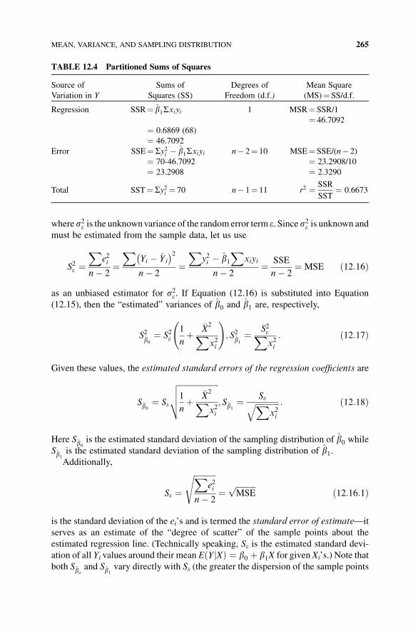
where s2e is the unknownvariance of the random error term e. Since s2e is unknown andmust be estimated from the sample data, let us use
S2e ¼X
e2i
n� 2¼X
Yi � Y i
� �2
n� 2¼X
y2i � b1X
xiyi
n� 2¼ SSE
n� 2¼ MSE ð12:16Þ
as an unbiased estimator for s2e . If Equation (12.16) is substituted into Equation
(12.15), then the “estimated” variances of b0 and b1 are, respectively,
S2b0
¼ S2e1
nþ
�X2
Xx2i
!; S2
b1¼ S2eX
x2i: ð12:17Þ
Given these values, the estimated standard errors of the regression coefficients are
Sb0¼ Se
ffiffiffiffiffiffiffiffiffiffiffiffiffiffiffiffiffiffiffiffi1
nþ
�X2
Xx2i
vuut ; Sb1¼ SeffiffiffiffiffiffiffiffiffiffiffiffiX
x2i
q : ð12:18Þ
Here Sb0is the estimated standard deviation of the sampling distribution of b0 while
Sb1is the estimated standard deviation of the sampling distribution of b1.Additionally,
Se ¼ffiffiffiffiffiffiffiffiffiffiffiX
e2i
n� 2
s
¼ffiffiffiffiffiffiffiffiffiffiMSE
pð12:16:1Þ
is the standard deviation of the ei’s and is termed the standard error of estimate—it
serves as an estimate of the “degree of scatter” of the sample points about the
estimated regression line. (Technically speaking, Se is the estimated standard devi-
ation of all Yi values around their mean E Y Xj Þ ¼ b0 þ b1Xð for given Xi’s.) Note that
both Sboand Sb1
vary directly with Se (the greater the dispersion of the sample points
TABLE 12.4 Partitioned Sums of Squares
Source of
Variation in Y
Sums of
Squares (SS)
Degrees of
Freedom (d.f.)
Mean Square
(MS)¼ SS/d.f.
Regression SSR¼ b1Sxiyi 1 MSR¼ SSR/1
¼ 46.7092
¼ 0.6869 (68)
¼ 46.7092
Error SSE¼Sy2i � b1Sxiyi n� 2¼ 10 MSE¼ SSE/(n� 2)
¼ 70-46.7092 ¼ 23.2908/10
¼ 23.2908 ¼ 2.3290
Total SST¼Sy2i ¼ 70 n� 1¼ 11 r2 ¼ SSR
SST¼ 0.6673
MEAN, VARIANCE, AND SAMPLING DISTRIBUTION 265
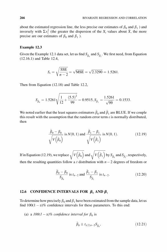
about the estimated regression line, the less precise our estimates of b0 and b1 ) andinversely with Sx2i (the greater the dispersion of the Xi values about �X, the more
precise are our estimates of b0 and b1 ).
Example 12.3
Given the Example 12.1 data set, let us find Sb0and Sb1
. We first need, from Equation
(12.16.1) and Table 12.4,
Se ¼ffiffiffiffiffiffiffiffiffiffiffiSSE
n� 2
r¼
ffiffiffiffiffiffiffiffiffiffiMSE
p¼
ffiffiffiffiffiffiffiffiffiffiffiffiffiffi2:3290
p¼ 1:5261:
Then from Equation (12.18) and Table 12.2,
Sb0¼ 1:5261
ffiffiffiffiffiffiffiffiffiffiffiffiffiffiffiffiffiffiffiffiffiffiffi1
12þ 5:5ð Þ2
99
s
¼ 0:9515; Sb1¼ 1:5261ffiffiffiffiffi
99p ¼ 0:1533:
We noted earlier that the least squares estimators b0 and b1 are BLUE. If we couplethis result with the assumption that the random error term e is normally distributed,
then
b0 � b0ffiffiffiffiffiffiffiffiffiffiffiffiffiffiV b0� �r is N 0; 1ð Þ and b1 � b1ffiffiffiffiffiffiffiffiffiffiffiffiffiffi
V b1� �r is N 0; 1ð Þ: ð12:19Þ
If in Equation (12.19), we replace
ffiffiffiffiffiffiffiffiffiffiffiffiffiffiV b0� �r
and
ffiffiffiffiffiffiffiffiffiffiffiffiffiffiV b1� �r
by Sb0and Sb1
, respectively,
then the resulting quantities follow a t distribution with n� 2 degrees of freedom or
b0 � b0Sb0
is tn�2 andb1 � b1Sb1
is tn�2: ð12:20Þ
12.6 CONFIDENCE INTERVALS FOR b0 AND b1
To determine howpreciselyb0 andb1 have been estimated from the sample data, let us
find 100(1� a)% confidence intervals for these parameters. To this end:
(a) a 100(1� a)% confidence interval for b0 is
b0 � ta=2;n�2Sb0; ð12:21Þ
266 BIVARIATE REGRESSION AND CORRELATION
(b) a 100(1� a)% confidence interval for b1 is
b1 � ta=2;n�2Sb1; ð12:22Þ
where� ta=2;n�2 and ta=2;n�2 are, respectively, the lower and upper percentage points
of the t distribution and 1� a is the confidence coefficient. Hence Equation (12.21)
informs us that wemay be 100(1� a)% confident that the true (population) regression
intercept b0 lies between b0 � ta=2;n�2Sb0; and Equation (12.22) tells us that we may
be 100(1� a)% confident that the true regression slope b1 lies between
b1 � ta=2;n�2Sb.
Example 12.4
Find 95% confidence intervals for b0 and b1 using the results of Examples 12.1
and 12.2. Given 1� a¼ 0.95, a/2¼ 0.025, and thus t0.025,10¼ 2.228. Then, via
Equation (12.21),
1:2221� 2:228 ð0:9515Þ! 1:2221� 2:1199! �0:8978; 3:3420ð Þ;
that is, we may be 95% confident that b0 lies between�0.8978 and 3.3420. And from
Equation (12.22),
0:6869� 2:228 ð0:1533Þ! 0:6869� 0:3416! 0:3453; 1:0285ð Þ;
so that we may be 95% confident that b1 lies between 0.3453 and 1.0285. So how
precisely have we estimated b0 and b1 ?We are within�2.1199 units of b0 with 95%reliability; and we are within �0.3416 units of b1 with 95% reliability. These results
may be stated in yet another fashion by using the “error bound” concept: we may be
95% confident that b0 will not differ from b0 bymore than�2.1199 units; andwemay
be 95% confident that b1 will not differ from b1 by more than �0.3416 units.
12.7 TESTING HYPOTHESES ABOUT b0 AND b1
How dowe know that X and Y are truly linearly related? Looked at in another fashion,
how do we know that X actually contributes significantly to the prediction of Y?
Answers to these questions can be garnered by way of testing a particular null
hypothesis against an appropriate alternative hypothesis.
Themost common type of hypothesis test is that of “no linear relationship between
X and Y” or E Y Xj Þ ¼ b0ð , that is, the conditional mean of Y given X does not depend
linearly on X. Hence the implied null hypothesis of “no linear relationship between X
and Y” is H0 : b1 ¼ 0. Possible alternative hypotheses are:
(a) If we are uncertain about the relationship between X and Y (we have no clue as
to whether or not these variables vary directly or inversely), then the
TESTING HYPOTHESES ABOUT b0 AND b1 267
appropriate alternative hypothesis is H1 : b1$0. Clearly, this alternative
implies a two-tail test with R ¼ t tj j ¼ b1=Sb1
������Hta=2;n�2
���on. If we reject
H0 in favor ofH1, then we can conclude that, at the 100a% level, there exists a
statistically significant linear relationship between X and Y.
(b) If, say, a priori theory indicates that X and Y are directly related, then we
chooseH1 : b1H0. This implies a one-tail test involving the right-hand tail of
the t distribution so thatR ¼ tf jt ¼ b1=Sb1Hta;n�2g. If we rejectH0 in favor of
H1, then we conclude that, at the 100a% level, there exists a statistically
significant positive linear relationship between X and Y.
(c) If, a priori theory indicates that X and Y are inversely related, then choose
H1 : b1G0. We now have a one-tail test involving the left-hand tail of the t
distribution so that R ¼ tf jt ¼ b1=Sb1G� ta;n�2g. If we reject H0 in favor of
H1, then we conclude that, at the 100a% level, there exists a statistically
significant negative linear relationship between X and Y.
(Note: if we do not reject H0, we cannot legitimately conclude that X and Y are
unrelated but only that there is no statistically significant “linear relationship”
exhibited by the data. The true underlying relationship between X and Y may be
highly nonlinear.)
As far as a test for the regression intercept b0 is concerned, we typically
test H0:b0¼ 0 (the population regression line passes through the origin) against
H1:b0 $ 0 or H1:b0 H 0 or H1:b0 G 0. The appropriate t test statistics and critical
regions are developed in a fashion similar to those specified above when testing
hypotheses about b1.
Example 12.5
Given the results obtained in Examples 12.1 and 12.2, determine if there exists
a statistically significant linear relationship between X and Y for a¼ 0.05.
Here H0:b1¼ 0 is tested against H1:b1 $ 0. In addition, ta/2,n� 2¼ t0.025,10¼ 2.228
and
tj j ¼ b1Sb1
�����
����� ¼0:6869
0:1533
����
���� ¼ 4:481:
Since R ¼ tf j tj jH2:228g, we can readily reject H0 in favor of H1—there exists a
statistically significant linear relationship between X and Y at the 5% level. (Here
p-value G 0.001.)
Could we have reached this conclusion by examining the confidence interval for
b1 provided in Example 12.4? The answer is, yes. The 95% confidence interval for
b1 contains all null hypotheses “not rejected” by a two-tail test at the 5% level.
Since zero is not a member of this confidence interval, the null hypothesis of b1¼ 0
is rejected.
268 BIVARIATE REGRESSION AND CORRELATION
Can we conclude that b1 ¼ b01 ¼ 0:475 at the a¼ 0.05 level? Here we will test
H0 : b1 ¼ b01 ¼ 0:475 against H1 : b1$b01 ¼ 0:475. Now our test statistic is
t ¼ b1 � b01Sb1
ð12:23Þ
with R ¼ tf j tj jHta=2;n�2g. For a¼ 0.05, t0.025,10¼ 2.228. Then, from Equation
(12.23),
tj j ¼ 0:6869� 0:475
0:1533
����
���� ¼ 1:3822:
Clearly, we are not within the critical region so that we cannot reject the null
hypothesis at the 5% level of significance. (Here 0.05 G p-value G 0.10.) Could
we have reached this conclusion by examining the confidence interval for b1?
12.8 PREDICTING THE AVERAGE VALUE OF Y GIVEN X
Suppose we are interested in predicting the average value of Y given X¼Xi, EðY XiÞ:jWith b0 and b1 unbiased estimators of b0 and b1, respectively, it follows that
EðYÞ ¼ Eðb0 þ b1XÞ ¼ b0 þ b1X, that is, an unbiased estimator for the population
regression line is the sample regression line. So with Y i ¼ b0 þ b1Xi an estimator for
EðYi XiÞ ¼ b0 þ b1Xij , it can be shown that the estimated standard deviation of Yi
may be computed as
SYi¼ Se
ffiffiffiffiffiffiffiffiffiffiffiffiffiffiffiffiffiffiffiffiffiffiffiffiffiffiffi1
nþ Xi � �Xð Þ2P
x2i
s
: ð12:24Þ
Under the assumption that e is normally distributed and b0 and b1 are BLUE, it
follows that
Y i � b0 þ b1Xið ÞSYi
is tn�2
and thus a 100(1� a)% confidence interval for E Yi Xij Þ ¼ b0 þ b1Xið is
Y i � ta=2;n�2SYi; ð12:25Þ
that is, we may be 100(1� a)% confident that the true or population average value of
Yi given Xi is bounded by the interval specified by Equation (12.25).
The interval determined by Equation (12.25) can be calculated for any Xi value.
And as we vary Xi, we generate a whole set of confidence intervals, with each one
centered around a point on the sample regression line. The collection of all these
PREDICTING THE AVERAGE VALUE OF Y GIVEN X 269
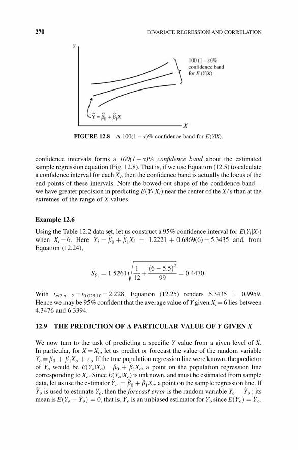
confidence intervals forms a 100(1� a)% confidence band about the estimated
sample regression equation (Fig. 12.8). That is, if we use Equation (12.5) to calculate
a confidence interval for each Xi, then the confidence band is actually the locus of the
end points of these intervals. Note the bowed-out shape of the confidence band—
we have greater precision in predicting E Yi Xij Þð near the center of the Xi’s than at the
extremes of the range of X values.
Example 12.6
Using the Table 12.2 data set, let us construct a 95% confidence interval for E Yi Xij Þðwhen Xi¼ 6. Here Y i ¼ b0 þ b1Xi ¼ 1.2221 þ 0.6869(6)¼ 5.3435 and, from
Equation (12.24),
SYi¼ 1:5261
ffiffiffiffiffiffiffiffiffiffiffiffiffiffiffiffiffiffiffiffiffiffiffiffiffiffiffiffiffiffiffi1
12þ 6� 5:5ð Þ2
99
s
¼ 0:4470:
With ta/2,n� 2¼ t0.025,10¼ 2.228, Equation (12.25) renders 5.3435 � 0.9959.
Hence we may be 95% confident that the average value of Y given Xi¼ 6 lies between
4.3476 and 6.3394.
12.9 THE PREDICTION OF A PARTICULAR VALUE OF Y GIVEN X
We now turn to the task of predicting a specific Y value from a given level of X.
In particular, for X¼Xo, let us predict or forecast the value of the random variable
Yo¼ b0 þ b1Xo þ eo. If the true population regression linewere known, the predictorof Yo would be E(Yo|Xo)¼ b0 þ b1Xo, a point on the population regression line
corresponding to Xo. Since E(Yo|Xo) is unknown, and must be estimated from sample
data, let us use the estimator Yo ¼ b0 þ b1Xo, a point on the sample regression line. If
Yo is used to estimate Yo, then the forecast error is the random variable Yo � Yo ; its
mean is EðYo � YoÞ ¼ 0; that is, Yo is an unbiased estimator for Yo since EðYoÞ ¼ Yo.
FIGURE 12.8 A 100(1� a)% confidence band for E(Y|X).
270 BIVARIATE REGRESSION AND CORRELATION
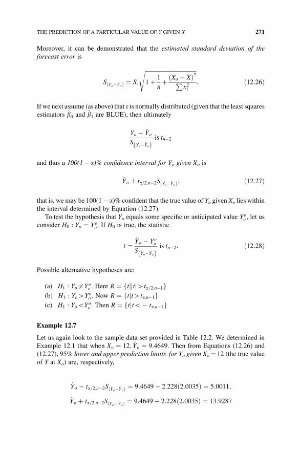
Moreover, it can be demonstrated that the estimated standard deviation of the
forecast error is
SðYo�YoÞ ¼ Se
ffiffiffiffiffiffiffiffiffiffiffiffiffiffiffiffiffiffiffiffiffiffiffiffiffiffiffiffiffiffiffiffiffiffiffiffi
1þ 1
nþ ðXo � �XÞ2P
x2i
s
: ð12:26Þ
If we next assume (as above) that e is normally distributed (given that the least squares
estimators b0 and b1 are BLUE), then ultimately
Yo � Yo
SYo�Yoð Þ
is tn�2
and thus a 100(1� a)% confidence interval for Yo given Xo is
Yo � ta=2;n�2SðYo�YoÞ; ð12:27Þ
that is, we may be 100(1� a)% confident that the true value of Yo given Xo lies within
the interval determined by Equation (12.27).
To test the hypothesis that Yo equals some specific or anticipated value Yoo , let us
consider H0 : Yo ¼ Yoo . If H0 is true, the statistic
t ¼ Yo � Yoo
SYo�Yoð Þ
is tn�2: ð12:28Þ
Possible alternative hypotheses are:
(a) H1 : Yo$Yoo . Here R ¼ tf j tj jHta=2;n�1g
(b) H1 : YoHYoo . Now R ¼ tf jtHta;n�1g
(c) H1 : YoGYoo . Then R ¼ tf jtG� ta;n�1g
Example 12.7
Let us again look to the sample data set provided in Table 12.2. We determined in
Example 12.1 that when Xo ¼ 12; Yo ¼ 9:4649. Then from Equations (12.26) and
(12.27), 95% lower and upper prediction limits for Yo given Xo¼ 12 (the true value
of Y at Xo) are, respectively,
Yo � ta=2;n�2SðYo�YoÞ ¼ 9:4649� 2:228 2:0035ð Þ ¼ 5:0011;
Yo þ ta=2;n�2SðYo�YoÞ ¼ 9:4649þ 2:228 2:0035ð Þ ¼ 13:9287
THE PREDICTION OF A PARTICULAR VALUE OF Y GIVEN X 271
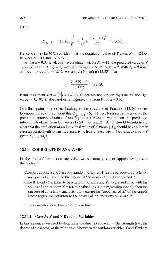
(Here
SðYo�YoÞ ¼ 1:5261
ffiffiffiffiffiffiffiffiffiffiffiffiffiffiffiffiffiffiffiffiffiffiffiffiffiffiffiffiffiffiffiffiffiffiffiffiffiffiffiffiffiffi
1þ 1
12þ ð12� 5:5Þ2
99
s
¼ 2:0035Þ:
Hence we may be 95% confident that the population value of Y given Xo¼ 12 lies
between 5.0011 and 13.9287.
At the a¼ 0.05 level, can we conclude that, for Xo¼ 12, the predicted value of Y
exceeds 9? HereH0: Yo¼ Yoo ¼ 9 is tested againstH1:YoH Yo
o ¼ 9.With Yo ¼ 9.4649
and ta,n� 2¼ t0.05,10¼ 1.812, we see, via Equation (12.28), that
t ¼ 9:4649� 9
2:0035¼ 0:2320
is not an element of R ¼ t tH1:812���
on. Hencewe cannot rejectH0 at the 5% level (p-
value H 0.10); Yo does not differ significantly from 9 for a¼ 0.05.
One final point is in order. Looking to the structure of Equation (12.24) versus
Equation (12.26), it is evident that SYo�Yoð ÞHSYi
. Hence, for a given 1� a value, theprediction interval obtained from Equation (12.26) is wider than the prediction
interval calculated from Equation (12.24). For any X¼Xo, it should be intuitively
clear that the prediction of an individual value of Y, namely Yo, should have a larger
error associatedwith it than the error arising from an estimate of the averagevalue ofY
given Xo, E(Y|Xo).
12.10 CORRELATION ANALYSIS
In the area of correlation analysis, two separate cases or approaches present
themselves:
CaseA:SupposeXandYareboth randomvariables.Then thepurposeof correlation
analysis is to determine the degree of “covariability” between X and Y.
Case B: If only Y is taken to be a random variable and Y is regressed on X, with the
values of non-random X taken to be fixed (as in the regression model), then the
purpose of correlation analysis is to measure the “goodness of fit” of the sample
linear regression equation to the scatter of observations on X and Y.
Let us consider these two situations in turn.
12.10.1 Case A: X and Y Random Variables
In this instance, we need to determine the direction as well as the strength (i.e., the
degree of closeness) of the relationship between the random variables X and Y, where
272 BIVARIATE REGRESSION AND CORRELATION
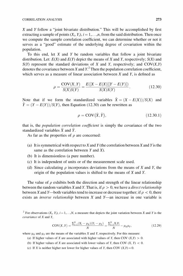
X and Y follow a “joint bivariate distribution.” This will be accomplished by first
extracting a sample of points (Xi, Yi), i¼ 1,. . .,n, from the said distribution. Then once
we compute the sample correlation coefficient, we can determine whether or not it
serves as a “good” estimate of the underlying degree of covariation within the
population.
To this end, let X and Y be random variables that follow a joint bivariate
distribution. Let: E(X) and E(Y) depict the means of X and Y, respectively; S(X) and
S(Y) represent the standard deviations of X and Y, respectively; and COV(X,Y)
denotes the covariance betweenX and Y.2 Then the population correlation coefficient,
which serves as a measure of linear association between X and Y, is defined as
r ¼ COV X; Yð ÞS Xð ÞS Yð Þ ¼ E X � E Xð Þ½ � Y � E Yð Þ½ �ð Þ
S Xð ÞS Yð Þ : ð12:30Þ
Note that if we form the standardized variables ~X ¼ X � E Xð Þð Þ=S Xð Þ and~Y ¼ Y � E Yð Þð Þ=S Yð Þ, then Equation (12.30) can be rewritten as
r ¼ COV ~X; ~Y� �
; ð12:30:1Þ
that is, the population correlation coefficient is simply the covariance of the two
standardized variables ~X and ~Y .As far as the properties of r are concerned:
(a) It is symmetrical with respect toX and Y (the correlation betweenX and Y is the
same as the correlation between Y and X).
(b) It is dimensionless (a pure number).
(c) It is independent of units or of the measurement scale used.
(d) Since calculating r incorporates deviations from the means of X and Y, the
origin of the population values is shifted to the means of X and Y.
The value of r exhibits both the direction and strength of the linear relationship
between the random variables X and Y. That is, if rH 0, we have a direct relationship
betweenX and Y—both variables tend to increase or decrease together; if rG 0, there
exists an inverse relationship between X and Y—an increase in one variable is
2 For observations (Xi, Yi), i¼ 1,. . .,N, a measure that depicts the joint variation between X and Y is the
covariance of X and Y,
COV X;Yð Þ ¼ SNi¼1 Xi � mXð Þ Yi � mYð Þ
N¼ SN
i¼1XiYi
N� mXmY ; ð12:29Þ
where mX and mY are the means of the variables X and Y, respectively. For this measure:
(a) If higher values of X are associated with higher values of Y, then COV (X,Y) H 0.
(b) If higher values of X are associated with lower values of Y, then COV (X, Y) G 0.
(c) If X is neither higher nor lower for higher values of Y, then COV (X,Y)¼ 0.
CORRELATION ANALYSIS 273
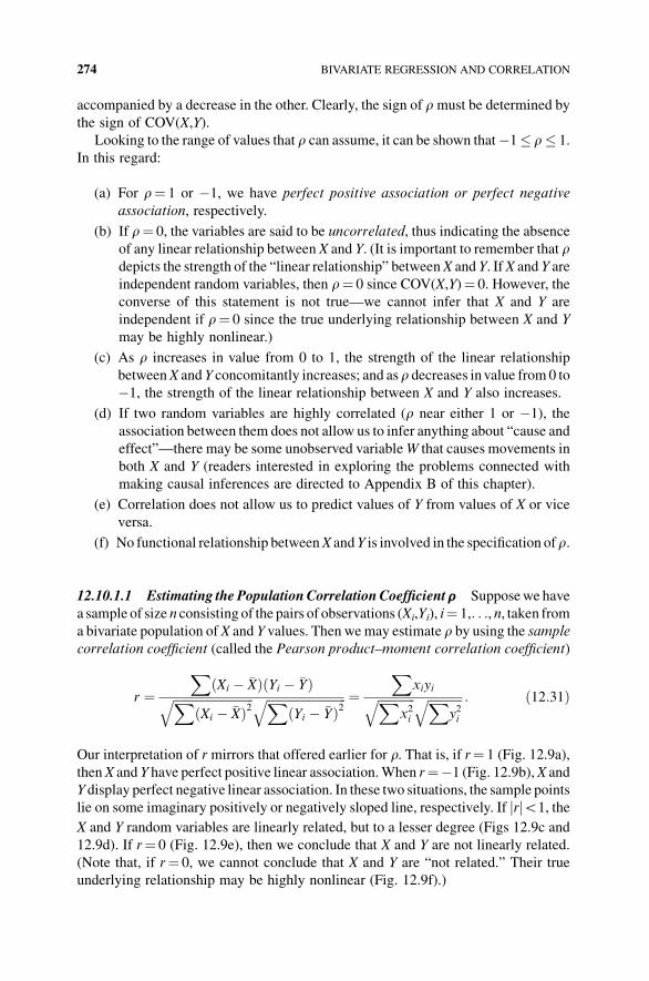
accompanied by a decrease in the other. Clearly, the sign of rmust be determined by
the sign of COV(X,Y).
Looking to the range of values that r can assume, it can be shown that�1� r� 1.
In this regard:
(a) For r¼ 1 or �1, we have perfect positive association or perfect negative
association, respectively.
(b) If r¼ 0, the variables are said to be uncorrelated, thus indicating the absence
of any linear relationship between X and Y. (It is important to remember that rdepicts the strength of the “linear relationship” betweenX and Y. IfX and Y are
independent random variables, then r¼ 0 since COV(X,Y)¼ 0. However, the
converse of this statement is not true—we cannot infer that X and Y are
independent if r¼ 0 since the true underlying relationship between X and Y
may be highly nonlinear.)
(c) As r increases in value from 0 to 1, the strength of the linear relationship
betweenX andY concomitantly increases; and asr decreases invalue from0 to
�1, the strength of the linear relationship between X and Y also increases.
(d) If two random variables are highly correlated (r near either 1 or �1), the
association between them does not allow us to infer anything about “cause and
effect”—there may be some unobserved variableW that causes movements in
both X and Y (readers interested in exploring the problems connected with
making causal inferences are directed to Appendix B of this chapter).
(e) Correlation does not allow us to predict values of Y from values of X or vice
versa.
(f) No functional relationship betweenX andY is involved in the specification ofr.
12.10.1.1 Estimating the PopulationCorrelation Coefficient r Supposewe have
a sample of size n consisting of the pairs of observations (Xi,Yi), i¼ 1,. . ., n, taken froma bivariate population of X and Y values. Then wemay estimate r by using the sample
correlation coefficient (called the Pearson product–moment correlation coefficient)
r ¼X
Xi � �Xð Þ Yi � �Yð ÞffiffiffiffiffiffiffiffiffiffiffiffiffiffiffiffiffiffiffiffiffiffiffiffiffiffiX
Xi � �Xð Þ2q ffiffiffiffiffiffiffiffiffiffiffiffiffiffiffiffiffiffiffiffiffiffiffiffiffiffiX
Yi � �Yð Þ2q ¼
XxiyiffiffiffiffiffiffiffiffiffiffiffiffiX
x2i
q ffiffiffiffiffiffiffiffiffiffiffiXy2i
q : ð12:31Þ
Our interpretation of r mirrors that offered earlier for r. That is, if r¼ 1 (Fig. 12.9a),
thenX and Y have perfect positive linear association.When r¼�1 (Fig. 12.9b),X and
Y display perfect negative linear association. In these two situations, the sample points
lie on some imaginary positively or negatively sloped line, respectively. If jrjG1, the
X and Y random variables are linearly related, but to a lesser degree (Figs 12.9c and
12.9d). If r¼ 0 (Fig. 12.9e), then we conclude that X and Y are not linearly related.
(Note that, if r¼ 0, we cannot conclude that X and Y are “not related.” Their true
underlying relationship may be highly nonlinear (Fig. 12.9f).)
274 BIVARIATE REGRESSION AND CORRELATION
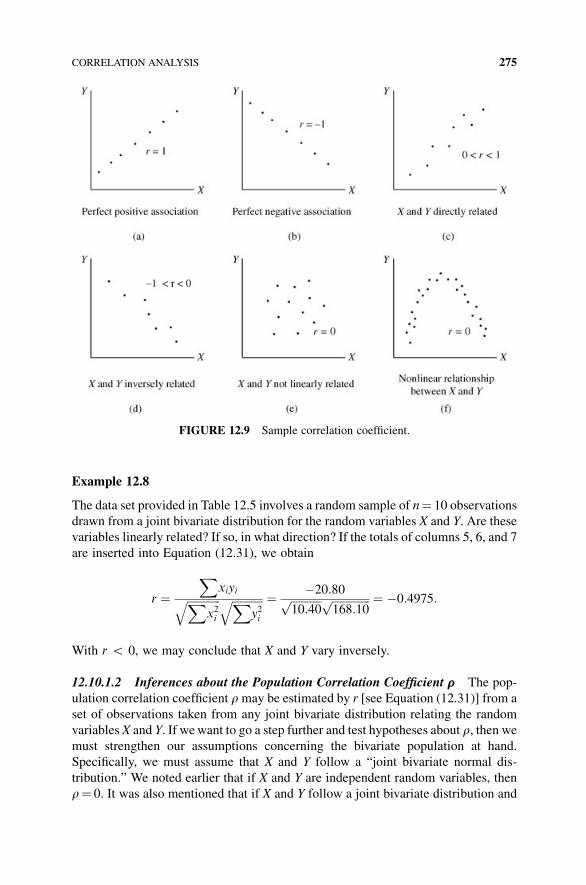
Example 12.8
The data set provided in Table 12.5 involves a random sample of n¼ 10 observations
drawn from a joint bivariate distribution for the random variables X and Y. Are these
variables linearly related? If so, in what direction? If the totals of columns 5, 6, and 7
are inserted into Equation (12.31), we obtain
r ¼X
xiyiffiffiffiffiffiffiffiffiffiffiffiffiXx2i
q ffiffiffiffiffiffiffiffiffiffiffiXy2i
q ¼ �20:80ffiffiffiffiffiffiffiffiffiffiffi10:40
p ffiffiffiffiffiffiffiffiffiffiffiffiffiffi168:10
p ¼ �0:4975:
With r G 0, we may conclude that X and Y vary inversely.
12.10.1.2 Inferences about the Population Correlation Coefficient r The pop-
ulation correlation coefficient rmay be estimated by r [see Equation (12.31)] from a
set of observations taken from any joint bivariate distribution relating the random
variables X and Y. If wewant to go a step further and test hypotheses about r, then wemust strengthen our assumptions concerning the bivariate population at hand.
Specifically, we must assume that X and Y follow a “joint bivariate normal dis-
tribution.” We noted earlier that if X and Y are independent random variables, then
r¼ 0. It was also mentioned that if X and Y follow a joint bivariate distribution and
FIGURE 12.9 Sample correlation coefficient.
CORRELATION ANALYSIS 275
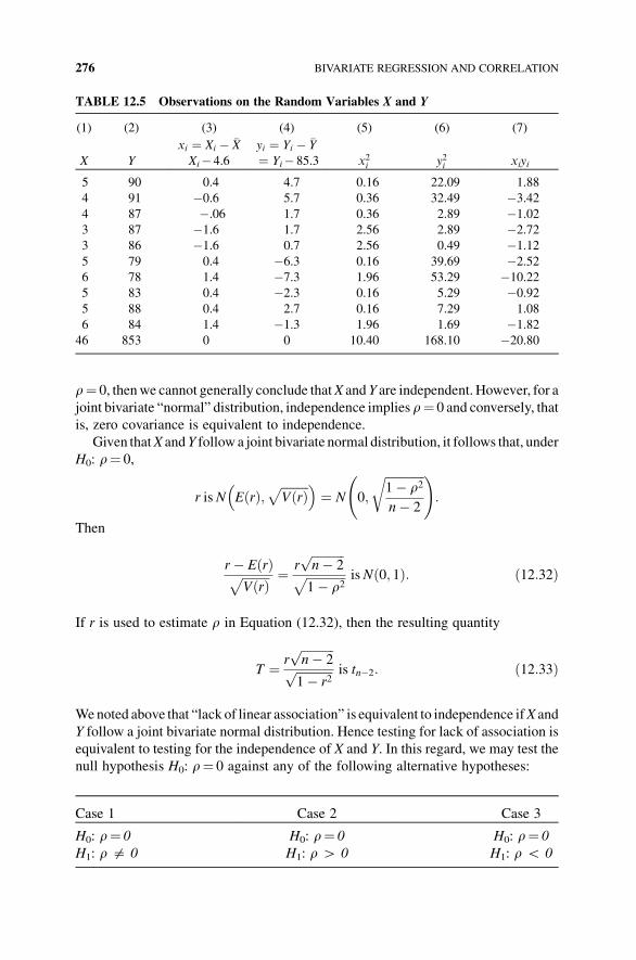
r¼ 0, thenwe cannot generally conclude thatX andY are independent. However, for a
joint bivariate “normal” distribution, independence implies r¼ 0 and conversely, that
is, zero covariance is equivalent to independence.
Given thatX andY follow a joint bivariate normal distribution, it follows that, under
H0: r¼ 0,
r is N E rð Þ;ffiffiffiffiffiffiffiffiffiV rð Þ
p� �¼ N 0;
ffiffiffiffiffiffiffiffiffiffiffiffiffi1� r2
n� 2
r !:
Then
r� E rð ÞffiffiffiffiffiffiffiffiffiV rð Þp ¼ r
ffiffiffiffiffiffiffiffiffiffiffin� 2
pffiffiffiffiffiffiffiffiffiffiffiffiffi1� r2
p isN 0; 1ð Þ: ð12:32Þ
If r is used to estimate r in Equation (12.32), then the resulting quantity
T ¼ rffiffiffiffiffiffiffiffiffiffiffin� 2
pffiffiffiffiffiffiffiffiffiffiffiffi1� r2
p is tn�2: ð12:33Þ
Wenoted above that “lack of linear association” is equivalent to independence ifX and
Y follow a joint bivariate normal distribution. Hence testing for lack of association is
equivalent to testing for the independence of X and Y. In this regard, we may test the
null hypothesis H0: r¼ 0 against any of the following alternative hypotheses:
Case 1 Case 2 Case 3
H0: r¼ 0 H0: r¼ 0 H0: r¼ 0
H1: r $ 0 H1: r H 0 H1: r G 0
TABLE 12.5 Observations on the Random Variables X and Y
(1) (2) (3) (4) (5) (6) (7)
X Y
xi ¼ Xi � �XXi� 4.6
yi ¼ Yi � �Y¼ Yi� 85.3 x2i y2i xiyi
5 90 0.4 4.7 0.16 22.09 1.88
4 91 �0.6 5.7 0.36 32.49 �3.42
4 87 �.06 1.7 0.36 2.89 �1.02
3 87 �1.6 1.7 2.56 2.89 �2.72
3 86 �1.6 0.7 2.56 0.49 �1.12
5 79 0.4 �6.3 0.16 39.69 �2.52
6 78 1.4 �7.3 1.96 53.29 �10.22
5 83 0.4 �2.3 0.16 5.29 �0.92
5 88 0.4 2.7 0.16 7.29 1.08
6 84 1.4 �1.3 1.96 1.69 �1.82
46 853 0 0 10.40 168.10 �20.80
276 BIVARIATE REGRESSION AND CORRELATION
The corresponding critical regions are determined as follows. At the 100a% level of
significance, the decision rules for rejecting H0 relative to H1 are:
Case 1: Reject H0 if Tj jHta=2;n�2 ð12:34aÞCase 2: Reject H0 if THta;n�2 ð12:34bÞCase 3: Reject H0 if TG� ta;n�2 ð12:34cÞ
Example 12.9
Given the data set appearing in Table 12.5, does our estimate for r, r¼�0.4975, lie
significantly below zero at the a¼ 0.05 level? From Equation (12.33),
T ¼ �0:4975ffiffiffi8
pffiffiffiffiffiffiffiffiffiffiffiffiffiffiffiffiffiffiffiffiffiffi1� 0:2475
p ¼ �1:6221
is not a member of R ¼ Tf jTG�t0:05;8 ¼ �1:86g. Hence we cannot reject H0 in
favor of H1—at the 5% level, the population correlation coefficient does not lie
significantly below zero. (Here 0.05 G p-value G 0.10.)
12.10.2 Case B: X Values Fixed, Y a Random Variable
We assumed in the preceding section that X and Y follow a joint bivariate normal
distribution. Let us, for the moment, retain that assumption here. In fact, under this
assumption, it can be shown that the population regression line has the form
E Yð jXÞ ¼ b0 þ b1X ¼ b0 þ rS Xð ÞS Yð ÞX: ð12:35Þ
Then if X and Y follow a joint bivariate normal distribution, r2 can be used as a
measure of the goodness of fit of the population regression line to the data points
(Xi, Yi), i¼ 1,. . .,n; it indicates the proportion of the variation in Y explained by the
linear influence of X as well as the “degree of covariability” between the random
variables X and Y. This same conclusion is valid if the assumption of normality is
dropped and the random variables X and Y simply follow a joint bivariate
distribution.
Now, if only Y is a random variable and the X values are held fixed (as was the case
when we developed our basic linear regression model earlier), then, since COV(X,Y)
does not exist, r2 (or r) cannot serve as a measure of covariability—it is only
indicative of the “goodness of fit” of the population regression line to the scatter of
sample points. Here’s the rub. If, under our previous set of regression assumptions (e is“well behaved”), we have obtained r2 according to
SSR
SST¼ b1
XxiyiXy2i
CORRELATION ANALYSIS 277
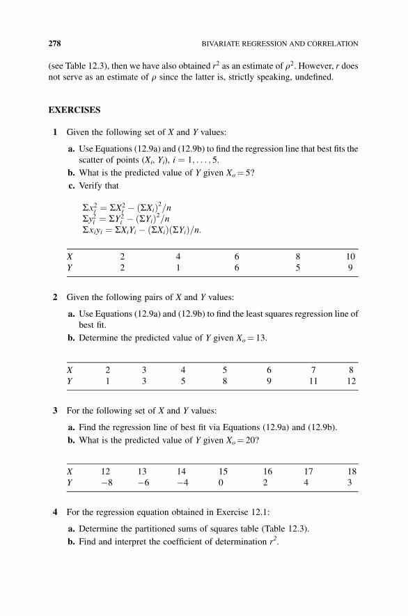
(see Table 12.3), then we have also obtained r2 as an estimate of r2. However, r doesnot serve as an estimate of r since the latter is, strictly speaking, undefined.
EXERCISES
1 Given the following set of X and Y values:
a. Use Equations (12.9a) and (12.9b) to find the regression line that best fits the
scatter of points (Xi, Yi), i ¼ 1; . . . ; 5.
b. What is the predicted value of Y given Xo¼ 5?
c. Verify that
Sx2i ¼ SX2i � SXið Þ2=n
Sy2i ¼ SY2i � SYið Þ2=n
Sxiyi ¼ SXiYi � SXið Þ SYið Þ=n:
X 2 4 6 8 10
Y 2 1 6 5 9
2 Given the following pairs of X and Y values:
a. Use Equations (12.9a) and (12.9b) to find the least squares regression line of
best fit.
b. Determine the predicted value of Y given Xo¼ 13.
X 2 3 4 5 6 7 8
Y 1 3 5 8 9 11 12
3 For the following set of X and Y values:
a. Find the regression line of best fit via Equations (12.9a) and (12.9b).
b. What is the predicted value of Y given Xo¼ 20?
X 12 13 14 15 16 17 18
Y �8 �6 �4 0 2 4 3
4 For the regression equation obtained in Exercise 12.1:
a. Determine the partitioned sums of squares table (Table 12.3).
b. Find and interpret the coefficient of determination r2.
278 BIVARIATE REGRESSION AND CORRELATION
5 For the regression equation obtained in Exercise 12.2:
a. Calculate the partitioned sums of squares table (Table 12.3).
b. Find and interpret the coefficient of determination r2.
6 For the regression equation obtained in Exercise 12.3:
a. Determine the partitioned sums of squares table (Table 12.3).
b. Calculate and interpret the coefficient of determination r2.
7 Suppose n¼ 30, �X ¼ 0:5; �Y ¼ 1;Sxiyi ¼ �30;Sx2i ¼ 10; and Sy2i ¼ 160:
a. Find the equation for the regression of Y on X.
b. Determine the partitioned sums of squares table.
c. Interpret the value of r2.
8 Given n ¼ 25;SXi ¼ 85;SYi ¼ 50;SX2i ¼ 625;SY2
i ¼ 228 and Sxiyi ¼ 30:
a. Find the equation for the regression of Y on X. [Hint: see part (c) of
Problem 12.1]
b. Determine the partitioned sums of squares table.
c. Find and interpret r2.
9 For the regression equation obtained in Exercise 12.7:
a. Find 95% confidence limits for b0 and b1.b. Test H0 : b0 ¼ 0 versusH1 : b0$0 for a¼ 0.05. What is your conclusion?
c. Test H0 : b1 ¼ 0 versusH1 : b1$0 for a¼ 0.05. What is your conclusion?
d. Can we conclude that b1 ¼ bo1 ¼ �3:7 at the 5% level? Set
H1 : b1$bo1 ¼ �3:7.
10 For the regression equation obtained in Exercise 12.8:
a. Find 99% confidence limits for b0 and b1.b. Test H0 : b0 ¼ 0 versusH1 : b0H0 for a¼ 0.01. What is your conclusion?
c. Test H0 : b1 ¼ 0 versusH1 : b1G0 for a¼ 0.01. What is your conclusion?
d. Can we conclude that b1 ¼ bo1 ¼ �0:25 at the 1% level? Set
H1 : b1$bo1 ¼ �0:25.
11 For the regression equation obtained in Exercise 12.1:
a. Find a 95% confidence interval for the average value of Y given Xo¼ 8.
b. Find a 95%confidence interval for predicting a single value ofY givenXo¼ 8.
12 For the regression equation obtained in Exercise 12.2:
a. Find a 95% confidence interval for the mean value of Y given Xo¼ 6.
b. Find a 95% prediction interval for a single value of Y given Xo¼ 6.
EXERCISES 279
13 Given n¼ 11, �X ¼ 4; �Y ¼ 20;Sx2i ¼ 64;Sy2i ¼ 1600; and Sxiyi ¼ 256 :
a. Determine the least squares regression equation.
b. What is the predicted value of Y for Xo¼ 6?
c. Find a 95% confidence interval for the average value of Y given Xo¼ 6.
d. Find a 95% prediction interval for a single value of Y given Xo¼ 6.
14 For the data set in Exercise 12.1:
a. Calculate the coefficient of correlation r [Equation (12.31)]. What
assumption is being made?
b. Test H0 : r ¼ 0 versusH1 : r$0 for a ¼ 0:05. What is your conclusion?
What assumption is being made?
15 For the data set in Exercise 12.2:
a. Calculate the correlation coefficient r via Equation (12.31).What assumption
is being made?
b. Test H0 : r ¼ 0 versusH1 : rH0 for a ¼ 0:01. What is your conclusion?
What assumption is being made?
16 For the data set in Exercise 12.3:
a. Find the correlation coefficient r. Under what assumption are your operating?
b. Test H0 : r ¼ 0 against H1 : rH0 for a ¼ 0:01. What is your conclusion?
What assumption are you making?
APPENDIX 12.A ASSESSING NORMALITY (APPENDIX 7.B
CONTINUED)
Appendix 7.B addressed the issue of determining if a simple random sample
taken from an unknown population is normally distributed. The approach offered
therein for assessing the normality of a data set was the normal probability
plot of the ordered observed sample data values against their normal scores in
the sample or their “expected” Z-scores (see Table 7.B.2 and Fig. 7.B.2). As
Fig. 7.B.2 reveals, we do obtain a fairly good approximation to a straight line (the
case of perfect normality). Is getting a “fairly good” approximation to a straight
line obtained by simply “eyeballing” the data points (Xj, Zpj ) (columns 3 and 4,
respectively, in Table 7.B.2) a satisfactory way to proceed? Can we devise a
more sophisticated approach to determining if a linear equation actually obtains?
And if one does obtain, can we test its statistical significance? To answer
these questions, one need only look to the developments in this chapter. The
task of assessing normality can be addressed via the application of regression
analysis.
280 BIVARIATE REGRESSION AND CORRELATION
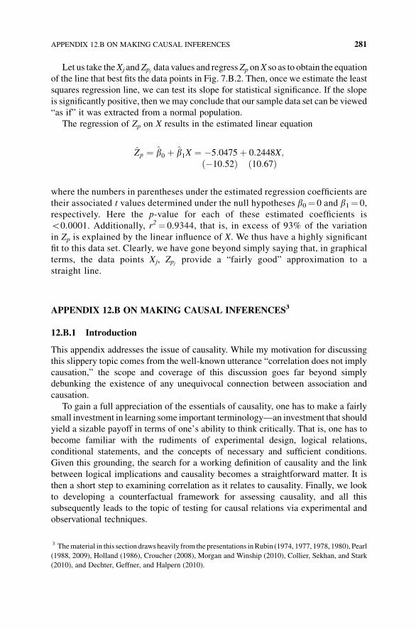
Let us take theXj and Zpj data values and regressZp onX so as to obtain the equation
of the line that best fits the data points in Fig. 7.B.2. Then, once we estimate the least
squares regression line, we can test its slope for statistical significance. If the slope
is significantly positive, then wemay conclude that our sample data set can be viewed
“as if” it was extracted from a normal population.
The regression of Zp on X results in the estimated linear equation
Zp ¼ b0 þ b1X ¼ �5:0475þ 0:2448X;�10:52ð Þ 10:67ð Þ
where the numbers in parentheses under the estimated regression coefficients are
their associated t values determined under the null hypotheses b0¼ 0 and b1¼ 0,
respectively. Here the p-value for each of these estimated coefficients is
G0.0001. Additionally, r2¼ 0.9344, that is, in excess of 93% of the variation
in Zp is explained by the linear influence of X. We thus have a highly significant
fit to this data set. Clearly, we have gone beyond simply saying that, in graphical
terms, the data points Xj, Zpj provide a “fairly good” approximation to a
straight line.
APPENDIX 12.B ON MAKING CAUSAL INFERENCES3
12.B.1 Introduction
This appendix addresses the issue of causality. While my motivation for discussing
this slippery topic comes from the well-known utterance “correlation does not imply
causation,” the scope and coverage of this discussion goes far beyond simply
debunking the existence of any unequivocal connection between association and
causation.
To gain a full appreciation of the essentials of causality, one has to make a fairly
small investment in learning some important terminology—an investment that should
yield a sizable payoff in terms of one’s ability to think critically. That is, one has to
become familiar with the rudiments of experimental design, logical relations,
conditional statements, and the concepts of necessary and sufficient conditions.
Given this grounding, the search for a working definition of causality and the link
between logical implications and causality becomes a straightforward matter. It is
then a short step to examining correlation as it relates to causality. Finally, we look
to developing a counterfactual framework for assessing causality, and all this
subsequently leads to the topic of testing for causal relations via experimental and
observational techniques.
3 Thematerial in this section draws heavily from the presentations inRubin (1974, 1977, 1978, 1980), Pearl
(1988, 2009), Holland (1986), Croucher (2008), Morgan and Winship (2010), Collier, Sekhan, and Stark
(2010), and Dechter, Geffner, and Halpern (2010).
APPENDIX 12.B ON MAKING CAUSAL INFERENCES 281
While the principal focus of this book is statistics, it is the case that there exists a
profound difference between statistical and causal concepts. Specifically:
(a) Statistical analysis: Employs estimation and testing procedures to determine
the parameters of a static probability distribution via sampling from that
distribution. Here one looks for associations, calculates the likelihood of
events, makes predictions, and so on. It is assumed that the experimental
conditions under which any inferences are made are invariant.
(b) Causal analysis: Designed to infer the likelihood of events through dynamic
changes induced by interventions or controlledmanipulations of some system.
So given, for instance, a static probability distribution, causal analysis provides
a framework for determining how the distribution would be affected if external
conditions would change; it incorporates additional suppositions that can identify
features of the distribution that remain invariant when controlled modifications
take place.
As was just mentioned, an important component of causal analysis is the notion
of an intervention. To perform a causal experiment, one must engage in a process
of external manipulation or intervention in order to determine the comparative
effects under different treatments on a group of subjects.4 Under this sort of
experimental policy, treatment is assigned to some subjects who would not
ordinarily seek treatment, and a placebo (the control) is given to some subjects
who would actually welcome treatment. Clearly, this approach is akin to short-
circuiting one behavioral process and rewiring it to another such process via a
splice formed by the act of randomization, for example, a coin flip determines who
actually enters the treatment group.
Looked at from an alternative perspective, suppose we have variables X and Y
and it is to be determined if X has an effect on Y. If we manipulate X and the
resulting response Y does not depend on the value assigned to X, then we can
conclude that X has no effect on Y. But if it is determined that the Y response
depends on the level assigned to X, then our conclusion is that X does have an effect
on Y. We thus need to consider the behavior of a system in a “disturbed state” that
is precipitated by some external intervention.
This “intervention theme” will emerge quite often in our discussion of causality,
especially when we get to counterfactuals. The next two sections house some
important definitional material.
12.B.2 Rudiments of Experimental Design
In statistics, it is generally accepted that observational studies (e.g., ones that simply
count the number of individuals with a specific condition or characteristic) can give
clues about, but can never fully confirm, cause and effect. The standard procedure for
testing and demonstrating causation is the randomized experiment.
4 Readers unfamiliar with this terminology can quickly read the next section.
282 BIVARIATE REGRESSION AND CORRELATION
We may view an experiment as a directed study designed to determine the effect
(if any) that varying at least one explanatory variable has on a response variable,
the variable of interest. These explanatory variables are called factors, and any
combination of the values of these factors is termed a treatment. An experimental
unit can be a person (called a subject), an object, a place or location, and so on.
To conduct a randomized experiment, the first step is to divide the totality of, say,
the subjects into two treatment groups: the experimental group (that receives the
treatment) and the control group (that is given a placebo—an inert or innocuous
substance such as a sugar tablet). It is the control group that bears the risk of being
exposed in some fashion to an activity different from that reserved for the exper-
imental group. Secondly, we must randomize the subjects to the treatment groups so
that the effect(s) of extraneous factors, which are beyond the control of
the experimenter, are minimized. Hence randomization “averages out” or tempers
the impact of variation attributed to factors that are not subject to manipulation.
Moreover, the randomized experiment must ideally be double blind—neither
the subject nor the experimenter knows what treatment is being administered to the
subject (it is not known by any party to the experiment whether a particular subject is
in the experimental group or in the control group).
As far as the control is concerned, its level or status is set at some fixed value for
the duration of the experiment. And regarding treatment levels for the experimental
group, they are manipulated or set at prespecified levels. These treatment levels
are the factors whose effect on the response variable is to be determined. Finally,
replication occurs when each treatment level is applied to more than one subject or
experimental unit.
For instance, suppose we are interested in measuring the impact of a new drug
(in pill form) on reducing “bad” cholesterol. Our subjects (each having a cholesterol
problem) can be randomly divided (by, say, the flip of a coin) into two groups: the
control, which received the placebo; and the experimental group, which receives
either 10, 20, or 40mg doses of the drug (again under randomization). Neither the
subjects nor the experimenter knowswho gets an inert pill or a specific treatment level
of the drug. Our goal is then to measure the effect of various treatment levels (relative
to the control and to each other) on the response variable (bad cholesterol level).
12.B.3 Truth Sets, Propositions, and Logical Implications
Suppose the realm of all logical possibilities L constitutes a set whose elements
correspond to propositions or statements. Think of a proposition as involving the
content or substance of meaning of any declarative sentence, which is taken to be
either true or false, but not both, for example, p can be the proposition “ice cream is
delicious.” Its negation, denoted p0, is “ice cream is not delicious.” So when p is true,
p0 is false; and when p is false, p0 is true.) For statements p and q in L, let the setsP and
Q represent the subsets of L for which these propositions are respectively true, that is,
P and Q are truth sets for statements p and q.
Let us assign truth values to propositions p and q. Specifically, if proposition p is
true,wewrite p¼ 1 (“1” denotes a proposition that is always true); and if proposition p
APPENDIX 12.B ON MAKING CAUSAL INFERENCES 283
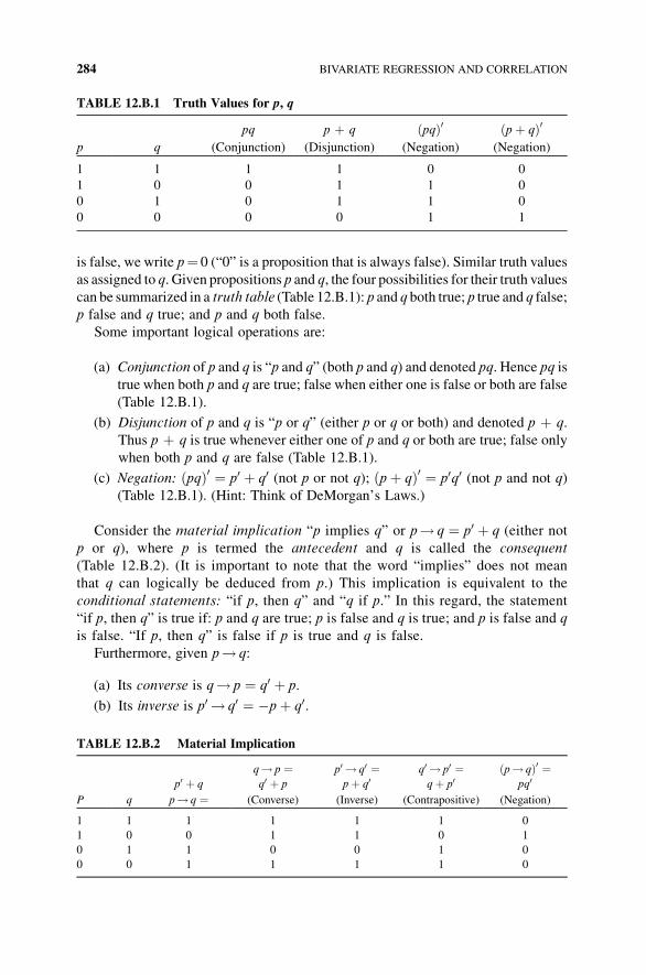
is false, we write p¼ 0 (“0” is a proposition that is always false). Similar truth values
as assigned to q. Given propositions p and q, the four possibilities for their truth values
can be summarized in a truth table (Table 12.B.1): p and q both true; p true and q false;
p false and q true; and p and q both false.
Some important logical operations are:
(a) Conjunction of p and q is “p and q” (both p and q) and denoted pq. Hence pq is
true when both p and q are true; false when either one is false or both are false
(Table 12.B.1).
(b) Disjunction of p and q is “p or q” (either p or q or both) and denoted p þ q.
Thus p þ q is true whenever either one of p and q or both are true; false only
when both p and q are false (Table 12.B.1).
(c) Negation: pqð Þ0 ¼ p0 þ q0 (not p or not q); pþ qð Þ0 ¼ p0q0 (not p and not q)
(Table 12.B.1). (Hint: Think of DeMorgan’s Laws.)
Consider the material implication “p implies q” or p! q ¼ p0 þ q (either not
p or q), where p is termed the antecedent and q is called the consequent
(Table 12.B.2). (It is important to note that the word “implies” does not mean
that q can logically be deduced from p.) This implication is equivalent to the
conditional statements: “if p, then q” and “q if p.” In this regard, the statement
“if p, then q” is true if: p and q are true; p is false and q is true; and p is false and q
is false. “If p, then q” is false if p is true and q is false.
Furthermore, given p! q:
(a) Its converse is q! p ¼ q0 þ p.
(b) Its inverse is p0 ! q0 ¼ �pþ q0.
TABLE 12.B.1 Truth Values for p, q
pq p þ q pqð Þ0 pþ qð Þ0p q (Conjunction) (Disjunction) (Negation) (Negation)
1 1 1 1 0 0
1 0 0 1 1 0
0 1 0 1 1 0
0 0 0 0 1 1
TABLE 12.B.2 Material Implication
q! p ¼ p0 ! q0 ¼ q0 ! p0 ¼ p! qð Þ0 ¼p0 þ q q0 þ p pþ q0 qþ p0 pq0
P q p! q ¼ (Converse) (Inverse) (Contrapositive) (Negation)
1 1 1 1 1 1 0
1 0 0 1 1 0 1
0 1 1 0 0 1 0
0 0 1 1 1 1 0
284 BIVARIATE REGRESSION AND CORRELATION
(c) Its contrapositive is q0 ! p0 ¼ qþ p0.(d) Its negation is p! qð Þ0 ¼ p0 þ qð Þ0 ¼ pq0.
(It is false that “p implies q” is “p and not q”).
The truth values for all these implications appear in Table 12.B.2.
12.B.4 Necessary and Sufficient Conditions
A statement p e P is a necessary condition for a statement q e Q to be true if q! p
(q implies p or “if q, then p”). Here “q is true only if p is true” so that p is a prerequisite
or requirement for q. So if we don’t have p, then we don’t have q. For instance,
“purchasing a ticket” (p) is a necessary condition for “admission to a concert” (q).
(If a person is present at a concert, they must have purchased a ticket, that is, q ! p.)
Additionally, a statement p e P is a sufficient condition for a statement q e Q to be
true if p ! q (p implies q or “if p, then q”). Thus “q is true if p is true.” Think of a
sufficient condition as a condition that, if satisfied, guarantees that q obtains or assures
the truth of q. That is,
“not bringing a camcorder to a concert” (p) is a sufficient condition for “admission
to the concert” (q).
(If a person does not bring a camcorder to a concert, they will be granted admission,
that is, p ! q.)
Note that having a ticket is not sufficient for admission—it is possible to have a
ticket and not be granted admission (a camcorder is discovered). And not having a
camcorder is not a necessary condition for admission—it is possible to not have a
camcorder and yet not be admitted (no ticket).
Let us consider another situation. The
“presence of water” is a necessary condition for “life on earth.”
(If life on earth exists, then that life has water.) However, the
“presence of water” is not a sufficient condition for “life on earth.”
(The presence of water does not, by itself, assure the existence of life since life also
needs oxygen and generally a myriad of favorable conditions for its support.)
Also,
“being male” is a necessary condition for “being a father.”
(If a person is a father, then that individual must be male.) But
“being male” is not a sufficient condition for “being a father.”
(One can be male and not have any children.)
APPENDIX 12.B ON MAKING CAUSAL INFERENCES 285
12.B.5 Causality Proper
Certainly everyone has, at one time or another, pondered the question “What caused a
particular event to occur?” This is not an easy question to answer. In fact, it is a
question thatmankind has been addressing for hundreds of years. If one starts with the
Western philosophical tradition, serious discussions of causation harken back to at
least Aristotle [see his Metaphysics, Books V, XI (350BC), tr. by W. D. Ross (1941)
and Posterior Analytics, Book II (350BC), tr. by E. S. Bouchier (1901)] and continue
with David Hume (1740, 1748), John Stuart Mill (1843), and, more recently, with
David Lewis (1973a, 1973b, 1973c, 1979, 1986), D. B. Rubin (1974, 1977, 1978,
1980), P. W. Holland (1986), and Judea Pearl (2009), among others.
We may view the notion of causality (or causation) as essentially a relationship
between “cause and effect,” that is, event A is said to cause event B if B is a
consequence of A—the causal event A is the reason why effect B occurs.5 Positing a
cause and effect relationship requires the following:
1. The cause must occur before the effect.
2. The cause must be connected to the effect in a probabilistic sense, that is, the
effect has a high probability of occurring.
3. There are no alternative or spurious causes due to so-called (unobserved)
lurking variables (more on this point later on).
(While this might be considered a na€ıve portrayal of cause and effect, a more
practicable version of this concept will be offered below.) Furthermore, we can
distinguish between:
(a) Necessary cause: Event A is a necessary cause of event B if the presence of B
implies the presence of A (the presence of A, however, does not imply that B
will occur).
(b) Sufficient cause: Event A is a sufficient cause of event B if the presence of A
implies the presence of B. However, another (confounding) event C may
possibly cause B. (Thus the presence of B does not imply the presence of A.)
Let us consider the features of these two causes in greater detail.
Necessary causality emphasizes the absence of alternative causes or processes that
are also capable of producing some effect. In this regard, this variety of causality is
useful when focusing on a specific event. And since various external or background
factors could also qualify as legitimate causal explanations, the isolation of a
necessary cause may be impeded because of confounding. For example, consider
the statement “A biking accident was the cause of Joe’s concussion.” Here we have a
specific scenario—a single-event causal assertion.
Sufficient causality involves the operation of a functioning causal process capable
of producing an effect. Here there exists a general or generic inclination for certain
5 The phrase “cause and effect” should always be understood to mean “alleged cause and alleged effect.”
286 BIVARIATE REGRESSION AND CORRELATION
types of events to generate other event types, where the particulars of event-specific
information are lacking. For instance, the assertion “biking accidents cause con-
cussions” is a generic causal statement.
12.B.6 Logical Implications and Causality
Do logical relations imply cause and effect? Suppose that for events A and Bwe have
the material implication A ! B. That is, A is a sufficient condition for B or B if A. For
concreteness, let events A and B appear as follows:
A: A person exhibits symptoms of Lyme disease.
B: A person was bitten by a deer tick.
For any individual under consideration, we can conclude that, ifA ! B, then from
column 3 of Table 12.B.2, “either notA orB” occurs (either the person does not exhibit
symptoms of Lyme disease or the person was bitten by a deer tick).
Is there a cause-and-effect relationship between events A and B? No, event A
cannot cause event B to occur (since symptoms of Lyme disease cannot cause a tick
bite). In sum, we can infer that “A implies B,” but certainly not that “A causes B;” we
cannot infer causality from just the observation of individuals (or, more generally,
from simply observing frequency data).
If conditional statements do not capture cause-and-effect relationships, then how
should we view the notion of cause and effect? A cause-and-effect assertion is
essentially a type of predictive hypothesis—a declaration that, if something changes
(under a distribution perturbation or intervention), you cannot eliminate the effect
without eliminating the cause. So given any adjustment that allows the cause to
remain, we can expect the effect to remain as well. For our purposes, we shall
recognize two forms of predictive hypotheses: a weak (or statistical) form; and a
strong (or causal) form. Specifically,
(a) [Statistical] For propositions p and q, not rejecting the hypothesis that
“p implies q” enables us to predict that, under repeated sampling from the
“same distribution,” we will continue to observe “either not p or q.”
(b) [Causal] For events A and B, the assertion that “A causes B” enables us to
predict that, if some intervention changes the distribution, thenwewill observe
“either not A or B” under repeated sampling from the “new distribution.”
Assertions about causality cannot be proved, only disproved. And causality is
disproved if we can eliminate the effect without eliminating the cause. For instance,
suppose that, day after day, the morning paper is delivered shortly after my morning
pot of coffee is brewed. Can we conclude that brewing coffee caused the paper to be
delivered? Obviously not. If the paper is not delivered because the carrier is taken ill
and the coffee is brewed as usual, then we have disproved the notion that brewing
coffee causes the paper to be delivered. (We have removed the effect but not the
APPENDIX 12.B ON MAKING CAUSAL INFERENCES 287
cause.) However, for events A and B given above, if the deer population is controlled
(decreased) and, ceteris paribus, the incidence of Lyme disease symptoms concom-
itantly decreases (albeit with a lag), then, since both of these eventsmove together, we
have not disproved anything, that is, we have not eliminated the effect without
eliminating the cause.
12.B.7 Correlation and Causality
In this chapter, we relied on the concept of correlation to determine if there exists a
degree of linear association between the two randomvariablesX andY. To this end,we
utilized the Pearson product–moment correlation coefficient r [Equation (12.29)] to
revealwhether a relationship is strong orweak andwhether it is positive or negative. If
the relationship is found to be statistically significant [via the test statistic (12.31)],
then regression analysis can subsequently be used to predict the value of one variable
(say, Y) from the value of the other variable (X). It was also mentioned that even if two
variables are significantly correlated, any such association does not imply causation.
Why is it the case that correlation does not imply causation? One possibility is that
the observed degree of association between X and Y is actually spurious or due to
confounding—we have false correlation due to the presence of an additional
unobserved or lurking variable that causes movements in both X and Y. For instance:
(a) Suppose we find that there exists a significant positive linear association
between the sale of bags of ice cubes and reported aggravated assaults. Will
increased sales of bags of ice cubes actually precipitate an increase in
aggravated assaults? Probably not. The explanation for this observed associ-
ation is that high temperatures and oppressive dew points increase this type of
aggressive behavior (people become much more irritable) as well as the sales
of ice cubes (people enjoy cool drinks in hot weather). Thus ice cube sales and
aggravated assaults are both affected by “temperature,” a lurking (third)
variable whose presence causes the observed correlation. Hence we are fooled
into thinking that ice cube sales and aggravated assaults are significantly
related.
(b) A study of school children found a significant positive linear association
between reading comprehension and shoe size. Does having big feet lead to
increased reading comprehension? It is not likely. It should be intuitively clear
that as children grow older, their reading comprehension and shoe size
concomitantly increase. Since a child’s mental and physical prowess both
develop as a child grows older, it is apparent that “age” is a lurking variable.
(c) A researcher found a high positive correlation between heavy drinking of
alcoholic beverages and respiratory problems. Does heavy drinking cause
respiratory difficulties? Not really. Since most heavy drinkers are also heavy
smokers, it is the lurking variable “heavy smoking” that leads to respiratory
problems. Thus heavy smoking is a confounder of heavy drinking and
respiratory problems.
288 BIVARIATE REGRESSION AND CORRELATION
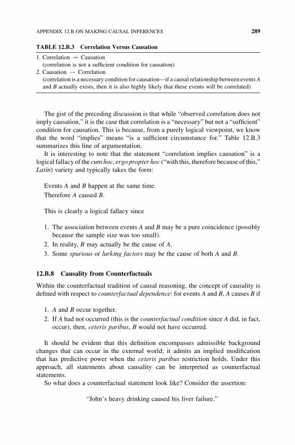
The gist of the preceding discussion is that while “observed correlation does not
imply causation,” it is the case that correlation is a “necessary” but not a “sufficient”
condition for causation. This is because, from a purely logical viewpoint, we know
that the word “implies” means “is a sufficient circumstance for.” Table 12.B.3
summarizes this line of argumentation.
It is interesting to note that the statement “correlation implies causation” is a
logical fallacy of the cumhoc, ergo propter hoc (“with this, therefore because of this,”
Latin) variety and typically takes the form:
Events A and B happen at the same time.
Therefore A caused B.
This is clearly a logical fallacy since
1. The association between events A and B may be a pure coincidence (possibly
because the sample size was too small).
2. In reality, B may actually be the cause of A.
3. Some spurious or lurking factors may be the cause of both A and B.
12.B.8 Causality from Counterfactuals
Within the counterfactual tradition of causal reasoning, the concept of causality is
defined with respect to counterfactual dependence: for events A and B, A causes B if
1. A and B occur together.
2. If A had not occurred (this is the counterfactual condition since A did, in fact,
occur), then, ceteris paribus, B would not have occurred.
It should be evident that this definition encompasses admissible background
changes that can occur in the external world; it admits an implied modification
that has predictive power when the ceteris paribus restriction holds. Under this
approach, all statements about causality can be interpreted as counterfactual
statements.
So what does a counterfactual statement look like? Consider the assertion:
“John’s heavy drinking caused his liver failure.”
TABLE 12.B.3 Correlation Versus Causation
1. Correlation =! Causation
(correlation is not a sufficient condition for causation)
2. Causation ! Correlation
(correlation is a necessary condition for causation—if a causal relationship between eventsA
and B actually exists, then it is also highly likely that these events will be correlated)
APPENDIX 12.B ON MAKING CAUSAL INFERENCES 289

Counterfactually, this statement is equivalent to
“Had John not been a heavy drinker, he would not have experienced liver failure.”
So for an actual cause-and-effect relationship to exist between events A and B, we
need something more than just a high degree of association between A and B
(item #1)—we also need these events to display a counterfactual dependence
(item #2).
For instance, suppose a student’s performance on a statistics exam was less than
stellar. After some reflection, he concludes that he did not solve enough practice
problems. Counterfactually, now think of this same student taking the same exam
under the same set of circumstances, but having solved awhole assortment of practice
exercises the night before the exam. This “controlled intervention” changes only one
small facet of the student’s situation—solving more practice problems. In this
circumstance, causation could be observed—we simply compare the exam scores
obtained with and without the extra problem solving. However, since this type of
experiment is impossible, causality can never be strictly proven, only inferred or
suggested. This discussion leads to the specification of the
Fundamental Problem of Causal Inference: It is impossible to directly observe
causal effects or outcomes.
Let us highlight the details of some of the subtleties underlying this fundamental
problem by considering another (and more sharply focused) example. Suppose that
each experimental unit (subject) in the population can be exposed to two alternative
states of a cause: the treatment; and the control. That is, the effect of one cause is
always specified relative to the effect of another cause. Hence the notion that “A
causesB”will be taken tomean thatA causesB relative to another cause that subsumes
the proposition “notA.”Hence one causewill be the treatment and the otherwill be the
control. Clearly, the control includes the condition “not the treatment A.”
For instance, high school seniors (the population of interest) are randomly assigned
to take a new accelerated SAT review course (the treatment) or not (the control). Here
we are implicitly assuming that each subject has a potential outcome under each
causal state although, in reality, each subject can be observed in only one such state
(either the treatment or the control) at a given point in time.
For this SAT review course (we are interested in the causal effect of taking or
not taking the SAT review course on the student’s SAT score), seniors who have
taken the review have theoretical “what-if scores” under the control state, and
seniors who have not taken the review have theoretical “what-if scores” under the
treatment state. Clearly, these “what-if outcomes” are unobservable counterfactual
outcomes.
Next, let Y be the response variable that measures the effect of a cause. (Here Y is
the SAT score.) In this regard, let us define the post-exposure values:
YT (s): The value of Y that would be observed if student s were exposed to the
treatment (the SAT review course).
290 BIVARIATE REGRESSION AND CORRELATION
YC(s): The value of Y that would be observed if student s were exposed to the
control (did not take the SAT review course).
Then for student s, the effect of the treatment relative to the effect of the control is
simply the difference
YTðsÞ � YCðsÞ: ð12:B:1Þ[The causal effect of the treatment relative to the control on student s as indexed
by y.]
Here the treatment causes the net effect in (12.B.1)—the difference between
observed and potential outcomes.
How may we determine the value of the causal effect provided by (12.B.1)? Note
that this difference is defined for a particular student s. Can we actually observe the
effects of causes for specific students? The answer is, no. We can never observe effect
(12.B.1) for a particular student s. This is because one can never observe the “what-if
outcome” under the treatment state for those subjects in the control state; and one can
never observe the “what-if outcome” under the control state for those subjects in the
treatment state. For a given student s, we cannot observe the values of both YT(s) and
YC(s) at the same time. [Remember that Equation (12.B.1) is actually the “what-if”
difference in achievement that could be calculated if student s could simultaneously be
in the SAT review course and not in the SAT review course.] Thus one can never
calculate subject-level causal states—the above-said fundamental problem of causal
influence. Thus individuals contribute outcome information only from the causal state
in which they are observed. Hence the typical response variable contains only a portion
of the information that would be needed to compute causal effects for all subjects.
This said, the fundamental problem does, however, admit a solution. While
individual causal effects (12.B.1) are unobserved, we can obtain the average causal
effect (using expectations) as
E YTðsÞ � YCðsÞ½ � ¼ E YTðsÞð Þ � E YCðsÞð Þ ¼ a: ð12:B:2Þ
Clearly, this difference is a “statistical solution” to the fundamental problem: we can
estimate an average causal effect a. And as long as the students are randomly assigned
to the treatment and control groups (YT (s) and YC (s) must be random variables),
Equation (12.B.2) is useful.
Given the above line of argumentation, it should by now be evident that causation
encompasses the assessment of behavior under interventions or controlled manip-
ulations. This observation is incorporated in the
General intervention principle: To infer a cause-and-effect relationship, we
need to determine how a distribution or system responds to interventions or
perturbations.
This principle now enables us to posit a workable definition of cause and effect.
Specifically, we first ask: “What can serve as a cause?” A cause is anything that could
conceivably be a treatment in a randomized experiment (e.g., various drug dosage
APPENDIX 12.B ON MAKING CAUSAL INFERENCES 291
levels, and so on) However, the attributes of a subject (sex, color, texture, and so on)
cannot serve as a cause in an experiment. In fact, attributes can only be used when
measuring association.
We next ask: “What can serve as a causal effect?” One may view an effect as an
empirical outcome that would emerge in a controlled randomized experiment—it
enables us to predict what circumstances would prevail under a hypothetical system
intervention.
The stage is now set for addressing the issue of “testing causality.” As will be
explained in Section 12.B.9, the so-called “gold standard” for a test of causality is the
implementation of a controlled randomized experiment. If performing this type of
experiment is impractical, then, as a second best option, an observational study might
be warranted.
12.B.9 Testing Causality
It is important to state at the outset that modeling for causal inferences emphasizes the
measurement of the “effects of causes.” Moreover, estimates of causal effects can be
obtained by performing controlled randomized experiments in which the sample
elements come under the direct control of, or are subject to manipulation by, the
experimenter.
Remember that it is the “controlled” randomized experiment that constitutes a
scientifically authenticated methodology for testing causality using sample data.
Uncontrolled experiments are anathema. For instance, suppose we are interested in
studying the ability of a newdrug to lower blood pressure inwomen. The effectiveness
of the drug depends upon both treatment and background factors (such as socioeco-
nomic conditions, and so on). Without a control, the choice of the treatment is at the
discretion of the subject—an obvious problem since we cannot then determine if
response rates are due to the treatment or due to extraneous conditions.
Remember also that the role of “randomization” is to simulate equality between
treatment and control groups. It is under randomization that the likelihood of these
groups having similar characteristics, save for some suitably restricted manipulation
or intervention, is rather high, that is, in the long run, randomization renders the
treatment and control groups equivalent in terms of all other possible effects on the
response so that any changes in response will reflect only the manipulation (treat-
ment). In fact, this likelihood increases with the number of participants in the
experiment. Now, if the measured difference between the effect of the treatment
relative to that of the control is found to be statistically significant, then it is also the
case that the likelihood of the treatment exerting a causal effect on some response
variable is quite high.
In short, we need to compare subjects with similar backgrounds so that treatment
effects can be isolated, and this is achieved under controlled randomized experi-
mentation. It is only through well-designed experiments that we can uncover, as
completely as possible, counterfactual dependencies between events.
While controlled randomized experiments are the cornerstone of causal analysis, it
may be the case that such experiments are impractical, too expensive, and/or conflict
292 BIVARIATE REGRESSION AND CORRELATION
with certain ethical or moral standards. For instance, suppose a subject with later-
stage cancer ends up in the control group of some double-blind experiment designed
to test the effect of a newly proposed cancer-curingwonder drug. And suppose further
that they think that, by virtue of participating in the study, a cure might actually be
forthcoming. What might be the reaction of these individuals if they found out that,
being in the control, only a placebo was issued and “a cure was not in the cards?”
Additionally, what if an experiment was designed to assess the impact of weight
gain on the speed of development of diabetes. Should subjects in the treatment group
be forced to gain weight while those in the control group are required to diet until
sufficient time passes so that their relative diabetes rates can be compared? How about
the issue of smoking as a contributing factor to the development of lung cancer?
Should subjects in the treatment group be required to smoke while subjects in the
control are prohibited from smoking so that, after some period of time, we can
determine if their relative cancer rates are significantly different? Clearly, most, if not
all, practitioners would have a problem with these types of treatments. So under any
moral or ethical restrictions, an alternative to a controlled randomized experiment is
the performance of an observational study to possibly infer causal effects. Before
exploring the efficacy of such studies, let us compare this form of inquiry with the
process of experimental design. Specifically:
Experimental study: All aspects of the system under study are controlled by the
experimenter (e.g., selection of experimental units, treatment(s), response
measurement procedures, and so on).
Observational study:While this is an empirical investigation of treatments and the
effects they cause, not all of the aforementioned particulars are under the control
of the investigator (e.g., randomized designs are infeasible—no control over
assigning treatments to subjects, and so on).
Can we rely on observational studies to infer causal effects? More formally, let us
look at the
Fundamental Question of Observational Analysis: Under what circumstances
can causal effects be inferred from statistical information obtained from
passive, intervention-free behavior?
In a nutshell, the answer is—“it is very difficult.” Conducting an observational
study to uncover causation is not a trivial task. For instance,
(a) Some researchers [see, in particular, D. A. Freedman (1991, 1999)] have
argued that relying primarily on statistical methodology can give questionable
results. One needs to make “causal assumptions;” and the ability to make
causal assumptions rests on subject matter expertise and good research design
to alleviate confounding and eliminate competing explanations of reality. In
fact, alternative explanations need to be tested.
APPENDIX 12.B ON MAKING CAUSAL INFERENCES 293
(b) Modeling assumptions (normality, randomness, homogeneity, independence,
and so on) must be tested. Only if the model itself passes muster, can we
squeeze some useful information from it.
(c) To drawcausal inferences fromobservational data, one needs to rely heavily on
intuition, intelligence, perseverance, and luck (possible confounders must be
identified, alternative paths of inquiry must be followed, a confluence of
evidence must be analyzed, elements of natural variability between subjects
must be identified, and so on).
(d) One must identify the process of causal exposure and how subjects end up in
alternative treatment states. How is the choice of treatment made? To answer
this, one must switch from a “treatment assignment” mindset to one focusing
on “treatment selection.”
(e) Large random-sample surveys are desirable (and it is assumed that within the
underlying population the relative proportion and pattern of exposure of
subjects to the causal process is fixed).
(f) If information about time is available, then a causal direction may possibly be
inferred. In this regard, cross-sectional data provides less information about the
direction and nature of causality than does longitudinal data.
It is important to note, however, that when it comes to observational studies,
all is not lost. Observational or non-experimental information can at times be
forthcoming from natural experiments, that is, experiments in which nature
provides the data in a fashion that is tantamount to the performance of a randomized
experiment. The classical case of a natural experiment is Snow’s observational
study of cholera [Snow (1855)]. Snow was able to conclude, via considerable effort
(door-to-door canvassing, brute-force elimination of confounders, and so on) that
nature itself had acted to mix subjects across treatments in a way that mirrors a
randomized controlled experiment. Hence persistent leg-work and the process of
elimination enabled Snow to eventually hit upon the notion that cholera is a water-
borne disease.
What is the bottom-line conclusion regarding observational studies and causality?
Observational studies can give hints or suggest directions, but can never fully
establish a cause-and-effect relationship.
12.B.10 Suggestions for Further Reading
Readers interested in causal studies pertaining to epidemiology and the health
effects of smoking should consult Friedman (1999), Freedman and Stark (1999),
Greenland (1998), Greenland and Brumback (2002), and Glymour and Greenland
(2008). A discussion pertaining to cause and effect in law and medicine can be
found in Austin (2008), Croucher (2008), Cole (1997), Rubin (2007), Collier, et al.
(2010), and Finkelstein and Levin (1990). Applications of causal inquiries in the
sciences are treated in Psillos (1999), Humphreys (1989, 2004), and Godfrey-
Smith (2003).
294 BIVARIATE REGRESSION AND CORRELATION
13AN ASSORTMENT OF ADDITIONALSTATISTICAL TESTS
13.1 DISTRIBUTIONAL HYPOTHESES
In Chapter 10, we assumed that a population probability distribution had a particular
functional form, for example, we assumed that a continuous random variable X was
N(m, s). Under this “distributional assumption,” we could then test a parametric
hypothesis about, say, the unknown mean m given that s is known. For instance, we
could test H0 : m ¼ mo, against H1 : mHmousing the standard normal distribution.
However, if the distributional assumption of normality is not made, then we can
actually test the distributional hypothesis H0 : X is normally distributed, against
H1 : Xis not normally distributed.
An important method of testing a distributional hypothesis is Pearson’s goodness-
of-fit test. Here we are interested in determining if a set of sample observations can be
viewed as values of a population random variable having a given probability
distribution. So given some distributional hypothesis, this test enables us to determine
if the population follows a specific probability model.
13.2 THE MULTINOMIAL CHI-SQUARE STATISTIC
We found in Chapter 5 that the essential characteristics of a binomial random
experiment are
Statistical Inference: A Short Course, First Edition. Michael J. Panik.� 2012 John Wiley & Sons, Inc. Published 2012 by John Wiley & Sons, Inc.
295
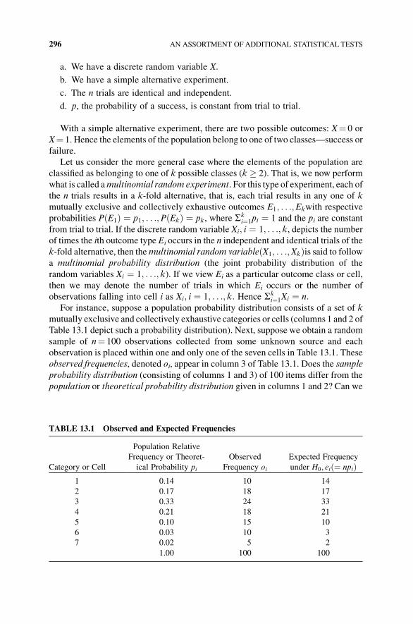
a. We have a discrete random variable X.
b. We have a simple alternative experiment.
c. The n trials are identical and independent.
d. p, the probability of a success, is constant from trial to trial.
With a simple alternative experiment, there are two possible outcomes: X¼ 0 or
X¼ 1. Hence the elements of the population belong to one of two classes—success or
failure.
Let us consider the more general case where the elements of the population are
classified as belonging to one of k possible classes (k � 2). That is, we now perform
what is called amultinomial random experiment. For this type of experiment, each of
the n trials results in a k-fold alternative, that is, each trial results in any one of k
mutually exclusive and collectively exhaustive outcomes E1; . . .;Ekwith respective
probabilities PðE1Þ ¼ p1; . . .;P Ekð Þ ¼ pk, where Ski¼1pi ¼ 1 and the pi are constant
from trial to trial. If the discrete random variable Xi; i ¼ 1; . . .; k, depicts the number
of times the ith outcome type Ei occurs in the n independent and identical trials of the
k-fold alternative, then themultinomial random variable X1; . . .;Xkð Þis said to followa multinomial probability distribution (the joint probability distribution of the
random variables Xi ¼ 1; . . .; k). If we view Ei as a particular outcome class or cell,
then we may denote the number of trials in which Ei occurs or the number of
observations falling into cell i as Xi; i ¼ 1; . . .; k: Hence Ski¼1Xi ¼ n:
For instance, suppose a population probability distribution consists of a set of k
mutually exclusive and collectively exhaustive categories or cells (columns 1 and 2 of
Table 13.1 depict such a probability distribution). Next, suppose we obtain a random
sample of n¼ 100 observations collected from some unknown source and each
observation is placed within one and only one of the seven cells in Table 13.1. These
observed frequencies, denoted oi, appear in column 3 of Table 13.1. Does the sample
probability distribution (consisting of columns 1 and 3) of 100 items differ from the
population or theoretical probability distribution given in columns 1 and 2? Can we
TABLE 13.1 Observed and Expected Frequencies
Category or Cell
Population Relative
Frequency or Theoret-
ical Probability pi
Observed
Frequency oi
Expected Frequency
under H0; ei ¼ npið Þ1 0.14 10 14
2 0.17 18 17
3 0.33 24 33
4 0.21 18 21
5 0.10 15 10
6 0.03 10 3
7 0.02 5 2
1.00 100 100
296 AN ASSORTMENT OF ADDITIONAL STATISTICAL TESTS
legitimately presume that the sample of 100 data points has been extracted from the
population probability distribution?
To determine if the observed or sample distribution is the same as the given
population distribution, let us test
H0: The population distribution and the sample distribution are identical
against
H1: The sample distribution differs from the population distribution.ð13:1Þ
HereH0 specifies the exact or theoretical distribution (our benchmark) andH1 simply
indicates some unspecified difference between these two distributions.
Given the relative frequencies listed for the population distribution (Table 13.1),
an exact multinomial probability can be obtained via a multinomial probability
calculation. However, since the direct calculation of multinomial probabilities
is, to say the least, quite tedious, an alternative approach will be offered that
enables us to easily address problems pertaining to goodness of fit. This alternative
computational scheme is based upon the Pearson multinomial chi-square
distribution.
In this regard, let the randomvariable X1; . . .;Xkð Þfollow amultinomial probability
distribution with parameters n, p1, . . ., pk. Then for fixed k, as the number of trials n
increases without bound, the distribution of the random variable
U ¼Xk
i¼1
Xi � npið Þ2npi
ð13:2Þ
[Pearson multinomial chi-square statistic]
approaches a chi-square distribution with k� 1 degrees of freedom (denoted w2k�1).
So if the possible outcomes of a random experiment can be decomposed into k
mutually exclusive and collectively exhaustive categories, with pi denoting the
probability that an outcome falls in category i, then, in n independent and identical
trials of this k-fold alternative experiment, with Xi representing the number of
outcomes favoring category i (so that Ski¼1Xi ¼ n), the distribution of U can be
approximated by a chi-square distribution with k� 1 degrees of freedom as n!¥.The importance of the quantity (Eq. 13.2) is that it can be used as a test statistic for
conducting a multinomial goodness-of-fit test. So for X1; . . .;Xkð Þa multinomial
random variable, we may test a null hypothesis that specifies the parameters of a
multinomial distribution as
H0 : p1 ¼ po1; . . .; pk ¼ pok ð13:3Þagainst
H1 : pi $ poi for at least one i ¼ 1; . . .; k:
Then for a random sample of size n taken from a multinomial population, Equation
(13.2) under H0 becomes
THE MULTINOMIAL CHI-SQUARE STATISTIC 297
Uo ¼Xk
i¼1
ðXi � npoi Þ2npoi
: ð13:4Þ
SinceUo is non-decreasing as i goes from 1 to k, we will reject H0 ifUo is an element
of the (upper tail) critical region R ¼ U UHw21�a;k�1
���on, where w21�a;k�1is the 100
(1� a) percentile of the chi-square distribution with k� 1 degrees of freedom and
a¼P (Type I Error). Clearly, we reject H0 for large Uo’s. As Equation (13.4)
reveals, a test of goodness of fit is essentially a test of a hypothesis concerning
specified cell probabilities pi, i¼ 1, . . ., k. It is important to remember that the use of
Equation (13.4) to approximate multinomial probabilities requires the following
conditions:
a. Each outcome falls into one and only one cell or category.
b. The outcomes are independent.
c. n is large.
13.3 THE CHI-SQUARE DISTRIBUTION
Having rationalized the test statistic for conducting a multinomial goodness-of-fit
test (Eq. 13.4), we next examine the properties of the chi-square distribution and its
attendant probabilities. The chi-square distribution is a continuous distribution
that represents the sampling distribution of a sum of squares of independent
standard normal variables. That is, if the observations X1, . . ., Xn constitute a
random sample of size n taken from a normal population with mean m and standard
deviation s, then the Zi¼ (Xi� m)/s, i¼ 1, . . ., n, are independent N(0,1) random
variables and
Y ¼Xn
i¼1
Z2i ¼
Xn
i¼1
Xi � mð Þ2s2
is w2n:
Looking to the properties of the chi-square distribution:
1. The mean and standard deviation of a chi-square random variable X are
E(X)¼ v andffiffiffiffiffiffiffiffiffiffiffiVðXÞp ¼ ffiffiffiffiffi
2vp
, respectively,where v denotes degrees of freedom.
2. The chi-square distribution is positively skewed and it has a peak that is sharper
than that of a normal distribution.
3. Selected quantiles of the chi-square distribution can be determined from the
chi-square table (Table A.3) for various values of the degrees of freedom
parameter v. For various cumulative probabilities 1� a (Fig. 13.1), the quantilew21�a;v satisfies
P X � w21�a;v
� �¼ 1� a
298 AN ASSORTMENT OF ADDITIONAL STATISTICAL TESTS
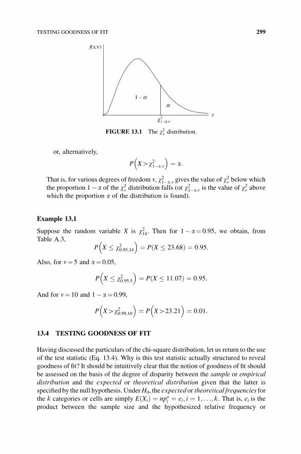
or, alternatively,
P XHw21�a;v
� �¼ a:
That is, for various degrees of freedom v, w21�a;v gives the value of w2v below which
the proportion 1� a of the w2v distribution falls (or w21�a;v is the value of w
2v above
which the proportion a of the distribution is found).
Example 13.1
Suppose the random variable X is w214. Then for 1� a¼ 0.95, we obtain, from
Table A.3,
P X � w20:95;14� �
¼ P X � 23:68ð Þ ¼ 0:95.
Also, for v¼ 5 and a¼ 0.05,
P X � w20:95;5� �
¼ P X � 11:07ð Þ ¼ 0:95.
And for v¼ 10 and 1� a¼ 0.99,
P XHw20:99;10� �
¼ P XH23:21� �
¼ 0:01.
13.4 TESTING GOODNESS OF FIT
Having discussed the particulars of the chi-square distribution, let us return to the use
of the test statistic (Eq. 13.4). Why is this test statistic actually structured to reveal
goodness of fit? It should be intuitively clear that the notion of goodness of fit should
be assessed on the basis of the degree of disparity between the sample or empirical
distribution and the expected or theoretical distribution given that the latter is
specified by the null hypothesis. UnderH0, the expected or theoretical frequencies for
the k categories or cells are simply E Xið Þ ¼ npoi ¼ ei; i ¼ 1; . . .; k: That is, ei is theproduct between the sample size and the hypothesized relative frequency or
FIGURE 13.1 The w2v distribution.
TESTING GOODNESS OF FIT 299
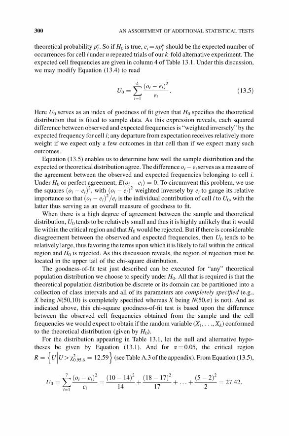
theoretical probability poi . So if H0 is true, ei¼ npoi should be the expected number of
occurrences for cell i under n repeated trials of our k-fold alternative experiment. The
expected cell frequencies are given in column 4 of Table 13.1. Under this discussion,
we may modify Equation (13.4) to read
U0 ¼Xk
i¼1
oi � eið Þ2ei
: ð13:5Þ
Here U0 serves as an index of goodness of fit given that H0 specifies the theoretical
distribution that is fitted to sample data. As this expression reveals, each squared
difference between observed and expected frequencies is “weighted inversely” by the
expected frequency for cell i; any departure from expectation receives relativelymore
weight if we expect only a few outcomes in that cell than if we expect many such
outcomes.
Equation (13.5) enables us to determine how well the sample distribution and the
expected or theoretical distribution agree. The difference oi� ei serves as ameasure of
the agreement between the observed and expected frequencies belonging to cell i.
Under H0 or perfect agreement, E oi � eið Þ ¼ 0: To circumvent this problem, we use
the squares oi � eið Þ2, with oi � eið Þ2 weighted inversely by ei to gauge its relative
importance so that oi � eið Þ2=ei is the individual contribution of cell i to U0, with the
latter thus serving as an overall measure of goodness to fit.
When there is a high degree of agreement between the sample and theoretical
distribution,U0 tends to be relatively small and thus it is highly unlikely that it would
liewithin the critical region and thatH0 would be rejected. But if there is considerable
disagreement between the observed and expected frequencies, then U0 tends to be
relatively large, thus favoring the terms uponwhich it is likely to fall within the critical
region and H0 is rejected. As this discussion reveals, the region of rejection must be
located in the upper tail of the chi-square distribution.
The goodness-of-fit test just described can be executed for “any” theoretical
population distribution we choose to specify under H0. All that is required is that the
theoretical population distribution be discrete or its domain can be partitioned into a
collection of class intervals and all of its parameters are completely specified (e.g.,
X being N(50,10) is completely specified whereas X being N(50,s) is not). And as
indicated above, this chi-square goodness-of-fit test is based upon the difference
between the observed cell frequencies obtained from the sample and the cell
frequencies we would expect to obtain if the random variable (X1, . . ., Xk) conformed
to the theoretical distribution (given by H0).
For the distribution appearing in Table 13.1, let the null and alternative hypo-
theses be given by Equation (13.1). And for a¼ 0.05, the critical region
R ¼ U UHw20:95;6 ¼ 12:59���
on(see Table A.3 of the appendix). From Equation (13.5),
U0 ¼X7
i¼1
oi � eið Þ2ei
¼ 10� 14ð Þ214
þ 18� 17ð Þ217
þ . . .þ 5� 2ð Þ22
¼ 27:42:
300 AN ASSORTMENT OF ADDITIONAL STATISTICAL TESTS
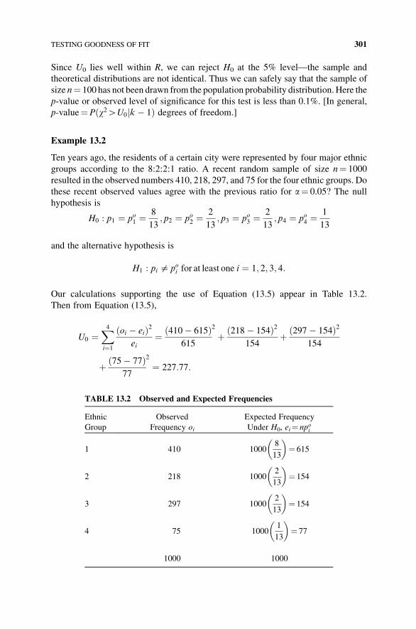
Since U0 lies well within R, we can reject H0 at the 5% level—the sample and
theoretical distributions are not identical. Thus we can safely say that the sample of
size n¼ 100 has not been drawn from the population probability distribution. Here the
p-value or observed level of significance for this test is less than 0.1%. [In general,
p-value¼Pðw2HU0 k � 1Þj degrees of freedom.]
Example 13.2
Ten years ago, the residents of a certain city were represented by four major ethnic
groups according to the 8:2:2:1 ratio. A recent random sample of size n¼ 1000
resulted in the observed numbers 410, 218, 297, and 75 for the four ethnic groups. Do
these recent observed values agree with the previous ratio for a¼ 0.05? The null
hypothesis is
H0 : p1 ¼ po1 ¼8
13; p2 ¼ po2 ¼
2
13; p3 ¼ po3 ¼
2
13; p4 ¼ po4 ¼
1
13
and the alternative hypothesis is
H1 : pi $ poi for at least one i ¼ 1; 2; 3; 4:
Our calculations supporting the use of Equation (13.5) appear in Table 13.2.
Then from Equation (13.5),
U0 ¼X4
i¼1
oi � eið Þ2ei
¼ 410� 615ð Þ615
2
þ 218� 154ð Þ2154
þ 297� 154ð Þ2154
þ 75� 77ð Þ77
2
¼ 227:77:
TABLE 13.2 Observed and Expected Frequencies
Ethnic
Group
Observed
Frequency oi
Expected Frequency
Under H0, ei¼ npoi
1 410 10008
13
� �¼ 615
2 218 10002
13
� �¼ 154
3 297 10002
13
� �¼ 154
4 75 10001
13
� �¼ 77
1000 1000
TESTING GOODNESS OF FIT 301
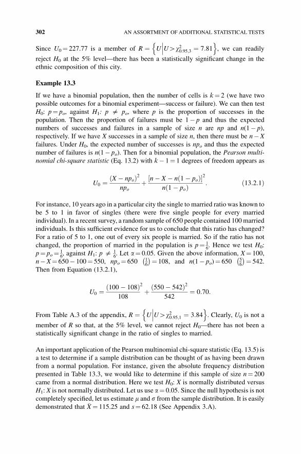
Since U0¼ 227.77 is a member of R ¼ U UHw20:95;3 ¼ 7:81���
on, we can readily
reject H0 at the 5% level—there has been a statistically significant change in the
ethnic composition of this city.
Example 13.3
If we have a binomial population, then the number of cells is k¼ 2 (we have two
possible outcomes for a binomial experiment—success or failure). We can then test
H0: p¼ po, against H1: p $ po, where p is the proportion of successes in the
population. Then the proportion of failures must be 1� p and thus the expected
numbers of successes and failures in a sample of size n are np and n(1� p),
respectively. If we have X successes in a sample of size n, then there must be n�X
failures. Under H0, the expected number of successes is npo and thus the expected
number of failures is n(1� po). Then for a binomial population, the Pearson multi-
nomial chi-square statistic (Eq. 13.2) with k� 1¼ 1 degrees of freedom appears as
U0 ¼ X � npoð Þ2npo
þ n� X � nð1� poÞ½ �nð1� poÞ
2
: ð13:2:1Þ
For instance, 10 years ago in a particular city the single to married ratio was known to
be 5 to 1 in favor of singles (there were five single people for every married
individual). In a recent survey, a random sample of 650 people contained 100married
individuals. Is this sufficient evidence for us to conclude that this ratio has changed?
For a ratio of 5 to 1, one out of every six people is married. So if the ratio has not
changed, the proportion of married in the population is p¼ 16. Hence we test H0:
p¼ po¼ 16, against H1: p $ 1
6. Let a¼ 0.05. Given the above information, X¼ 100,
n�X¼ 650� 100¼ 550, npo¼ 650 16
� ¼ 108, and n(1� po)¼ 650 56
� ¼ 542.
Then from Equation (13.2.1),
U0 ¼ 100� 108ð Þ108
2
þ 550� 542ð Þ2542
¼ 0:70:
From Table A.3 of the appendix, R ¼ U UHw20:95;1 ¼ 3:84���
on. Clearly, U0 is not a
member of R so that, at the 5% level, we cannot reject H0—there has not been a
statistically significant change in the ratio of singles to married.
An important application of the Pearson multinomial chi-square statistic (Eq. 13.5) is
a test to determine if a sample distribution can be thought of as having been drawn
from a normal population. For instance, given the absolute frequency distribution
presented in Table 13.3, we would like to determine if this sample of size n¼ 200
came from a normal distribution. Here we test H0: X is normally distributed versus
H1: X is not normally distributed. Let us use a¼ 0.05. Since the null hypothesis is not
completely specified, let us estimate m and s from the sample distribution. It is easily
demonstrated that �X¼ 115.25 and s¼ 62.18 (See Appendix 3.A).
302 AN ASSORTMENT OF ADDITIONAL STATISTICAL TESTS
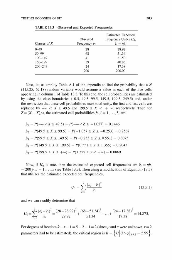
Next, let us employ Table A.1 of the appendix to find the probability that a N
(115.25, 62.18) random variable would assume a value in each of the five cells
appearing in column 1 of Table 13.3. To this end, the cell probabilities are estimated
by using the class boundaries (–0.5, 49.5, 99.5, 149.5, 199.5, 249.5) and, under
the restriction that these cell probabilities must total unity, the first and last cells are
replaced by –¥ G X � 49.5 and 199.5 � X G þ ¥, respectively. Then for
Z¼ X � �Xð Þ=s, the estimated cell probabilities pi; i ¼ 1; . . .; 5, are
p1 ¼ Pð�¥GX � 49:5Þ ¼ Pð�¥GZ � �1:057Þ ¼ 0:1446
p2 ¼ P 49:5 � X � 99:5ð Þ ¼ P �1:057 � Z � �0:253ð Þ ¼ 0:2567
p3 ¼ P 99:5 � X � 149:5ð Þ ¼ P �0:253 � Z � 0:551ð Þ ¼ 0:3075
p4 ¼ P 149:5 � X � 199:5ð Þ ¼ P 0:551 � Z � 1:355ð Þ ¼ 0:2043
p5 ¼ P 199:5 � X � þ¥ð Þ ¼ Pð1:355 � ZGþ¥Þ ¼ 0:0869:
Now, if H0 is true, then the estimated expected cell frequencies are ei ¼ npi¼ 200 pi; i ¼ 1; . . .; 5 (see Table 13.3). Then using a modification of Equation (13.5)
that utilizes the estimated expected cell frequencies,
U0 ¼Xk
i¼1
oi � eið Þ2ei
ð13:5:1Þ
and we can readily determine that
U0¼X5
i¼1
oi� eið Þ2ei
¼ 28�28:92ð Þ228:92
þ 68�51:34ð Þ251:34
þ ...þ 24�17:38ð Þ217:38
¼14:875:
For degrees of freedom k� r� 1¼ 5� 2� 1¼ 2 (since m and swere unknown, r¼ 2
parameters had to be estimated), the critical region is R ¼ U UHw20:95;2 ¼ 5:99���
on.
TABLE 13.3 Observed and Expected Frequencies
Classes of X
Observed
Frequency oi
Estimated Expected
Frequency Under H0,
ei ¼ npi
0–49 28 28.92
50–99 68 51.34
100–149 41 61.50
150–199 39 40.86
200–249 24 17.38
200 200.00
TESTING GOODNESS OF FIT 303
Since U0 exceeds 5.99, we can reject the null hypothesis that the sample was drawn
from a normal population; at the 5% level the normal distribution does not provide a
good fit to the sample data.
It is important to note that if X is a continuous random variable, then to use this
chi-square goodness-of-fit test, the data must be grouped into k classes or cells of
uniform length, where the number of cells typically ranges between 5 and 10 and
each cell has an expected frequency of at least 5. If it should happen that the
expected frequency in any cell is less than 5, then adjacent cells or classes should
be combined so that all the expected frequencies will be at least 5, since otherwise
the approximation will not be adequate. Note also that degrees of freedom will be
k� 1 less the number of parameters (r) we have to estimate in order to determine
the ei ’s, i¼ 1, . . ., k.
13.5 TESTING INDEPENDENCE
In the Pearson chi-square tests covered in the preceding section, the random
sample data were classified via a single criterion into a set of mutually exclusive
and collectively exhaustive categories or cells. However, as will be demonstrated
shortly, this approach can be applied to situations other than these resulting from
multinomial experiments. For example, suppose our observations are classified
according to two or more attributes. Then the question naturally arises: “Are these
attributes or categories of classification statistically independent?” (“Do they lack
statistical association?”) To answer this, we shall look to Pearson’s chi-square test
for independence of attributes or Pearson’s chi-square test of association. As will
be evidenced below, this technique can be applied to either quantitative or
qualitative data.
Given a specific criterion of classification, suppose we cross-classify our data set
according to a second criterion or attribute, where the population proportion within
each resulting cell is unknown, for example, given a set of categories on the factor
“educational attainment” (high school diploma, college degree, graduate school
degree), we may cross-classify according to a second factor such as “sex” or “income
level” (low, medium, high). We shall refer to the resulting two-way classification
scheme as a two-way contingency table.
As stated above, we are interested in determining whether there is any
dependency relationship or association between two population characteristics.
We thus test
H0 : The two attributes are independent or the rows and columns representðindependent classificationsÞ
against
H1 : The two attributes are not independent or the rows and columnsðare not independent classificationsÞ: ð13:6Þ
304 AN ASSORTMENT OF ADDITIONAL STATISTICAL TESTS
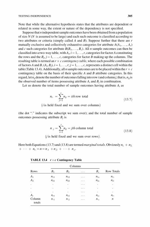
Note that while the alternative hypothesis states that the attributes are dependent or
related in some way, the extent or nature of the dependency is not specified.
Suppose thatn independent sample outcomeshavebeenobtained fromapopulation
of size N (N is assumed to be large) and each such outcome is classified according to
two attributes or criteria (simply called A and B). Suppose further that there are r
mutually exclusive and collectively exhaustive categories for attribute A(A1, . . ., Ar)
and c such categories for attribute B(B1, . . ., Bc). All n sample outcomes can then be
classified into a two-way table, withAi, i¼ 1, . . ., r, categories for factorA constituting
the rows and the Bj, j¼ 1, . . ., c, categories for factor B making up the columns. The
resulting table is termed an r� c contingency table, where each possible combination
of factorsA andB, (Ai,Bj), i¼ 1, . . ., r; j¼ 1, . . ., c, represents a distinct cell within thetable (Table 13.4).Additionally, alln sampleoutcomes are to beplacedwithin the r� c
contingency table on the basis of their specific A and B attribute categories. In this
regard, letnijdenote thenumberofoutcomes falling into row iandcolumn j, that is,nij is
the observed number of items possessing attribute Ai and Bj in combination.
Let us denote the total number of sample outcomes having attribute Ai as
ni � ¼Xc
j¼1
nij ¼ ith row total
i is held fixed and we sum over columnsð Þð13:7Þ
(the dot “.” indicates the subscript we sum over); and the total number of sample
outcomes possessing attribute Bj is
n � j ¼Xr
i¼1
nij ¼ jth column total
j is held fixed and we sum over rowsð Þ:ð13:8Þ
Here both Equations (13.7) and (13.8) are termedmarginal totals. Obviously ni. þ n2.þ � � � þ nr.¼ n¼ n.1 þ n.2 þ � � � þ n.c.
TABLE 13.4 r� c Contingency Table
Columns
Rows B1 B2 . . . Bc Row Totals
A1 n11 n12 . . . n1c n1.
A2 n21 n22 . . . n2c n2.
. . . . . . . .
. . . . . . . .
. . . . . . . .
Ar nr1 nr2 . . . nrc nr.
Column
totals
n.1 n.2 . . . n.c n
TESTING INDEPENDENCE 305
As stated in Equation (13.6), the null hypothesis is that factors A and B are
independent. UnderH0, these factors for the population at large are independent if and
only if
PðAi \ BjÞ ¼ P Aið Þ �P Bj
� ; i ¼ 1; . . .; r; j ¼ 1; . . .; c ð13:9Þ
for all possible joint events Ai \ Bj [see Section 4.4 and Equation (4.7)] or
pij ¼ pi �ð Þ p � j�
; i ¼ 1; . . .; r; j ¼ 1; . . .; c: ð13:9:1Þ
Here pij is the unknown joint probability that an item selected at random from the
population will be from cell (i, j), pi. is the unknownmarginal probability that an item
drawn at random from the population is from category i of characteristic A, and p.j is
the unknown marginal probability that a randomly selected item from the population
is from category j of characteristic B. Then under the independence assumption,
Equation (13.6) can be rewritten as
H0 : pij ¼ pi �ð Þ p � j�
for all i and j; and
H1 : pij$ pi �ð Þ p � j�
for at least one cell ði; jÞ; i ¼ 1; . . .; r; j ¼ 1; . . .; c:ð13:6:1Þ
Given that the populationmarginal probabilities pi. and p.j are unknown, the estimated
sample marginal probabilities can be obtained as
pi � ¼ni �n
; i ¼ 1; . . .; r; ð13:10aÞ
p � j ¼n � jn
; j ¼ 1; . . .; c ð13:10bÞ
respectively. Hence the estimated population probability of the joint event Ai \ Bj is
pij ¼ pi �ð Þ p � j� �
¼ ni �ð Þ n � j�
n2for all i; j ð13:11Þ
and thus the expected frequency of the joint event Ai \ Bj must be
eij ¼ npij ¼ni �ð Þ n � j
�
nfor all i; j: ð13:12Þ
So in a test of independence of attributes, the expected frequency in cell (i, j) is simply
the product between the marginal total for row i and the marginal total for column j
divided by the sample size n.
On the basis of Equation (13.12), we can extend Pearson’s multinomial chi-square
statistic (Eq. 13.2) to the casewherewe test for independence among two factorsA and
B in an r� c contingency table. To this end, for n independent trials of a random
306 AN ASSORTMENT OF ADDITIONAL STATISTICAL TESTS
experiment classified by the categories of attributesA andB, if the random variableXij
is the frequency of event Ai \ Bj, then the statistic
U ¼Xr
i¼1
Xc
j¼1
Xij � npij� 2
npijð13:13Þ
is, for large n, approximately chi-square distributed with rc� 1 degrees of freedom.
Under Equation (13.6.1), with Equations (13.10)–(13.12) holding, Equation (13.13)
becomes the Pearson chi-square statistic for a test of association
U0 ¼Xr
i¼1
Xc
j¼1
nij � npij
� �2
npij
¼Xr
i¼1
Xc
j¼1
oij � eij� 2
eij;
ð13:14Þ
where oij (¼ nij) is the observed frequency for cell (i, j). For largen, Equation (13.14) is
approximately chi-square distributed with (r� 1)(c� 1) degrees of freedom. How
have we determined degrees of freedom for Equation (13.14)? Since we estimate
marginal probabilities from sample outcomes, we subtract 1 degree of freedom for
each parameter estimated. Since Sri¼1pi� ¼ 1 ¼ Sc
j¼1pj� , there are, respectively, r� 1
row parameters and c – 1 column parameters to be estimated. Hence it follows that
degrees of freedom¼ rc� 1� (r� 1)� (c� 1)¼ (r� 1)(c� 1).
Note that the finite double sum in Equation (13.14) has us calculate the grand total
over all r� c cells, with the contribution of the (i, j)th cell to the Pearson chi-square
statistic being (oij� eij)2/eij. As was the case with Equation (13.2), we compare the
observed cell frequencies with the expected cell frequencies under H0. If the
deviations between the observed and expected cell frequencies are larger than that
which could be attributed to sampling variation alone, then we are inclined to reject
H0 for large values of U0. Hence the critical region for this upper tail test is
R ¼ U UHw21�a; r�1ð Þ c�1ð Þ���
on, where w21�a; r�1ð Þ c�1ð Þis the 100(1� a) percentile of the
chi-square distribution with (r� 1)(c� 1) degrees of freedom and a¼P(TIE). It is
important to mention that in order for the Pearson chi-square statistic to provide a
good approximation to the chi-square distribution with (r� 1)(c� 1) degrees of
freedom, each expected cell frequency should be at least 5. If this requirement is not
met, then adjacent cells can be combined as is appropriate.
Example 13.4
Suppose the principal (Miss Apple) of the ABC Elementary School is contemplating
the imposition of a new dress code for children in grades 1 to 6. She has decided to
sample the opinion of all “interested parties” in order to determinewhether opinion on
this issue is independent of school affiliation. A random sample of n¼ 300 interested
TESTING INDEPENDENCE 307
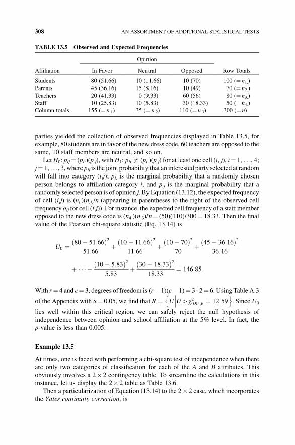
parties yielded the collection of observed frequencies displayed in Table 13.5, for
example, 80 students are in favor of the new dress code, 60 teachers are opposed to the
same, 10 staff members are neutral, and so on.
LetH0: pij¼ (pi.)(p.j), withH1: pij$ (pi.)(p.j) for at least one cell (i, j), i¼ 1, . . ., 4;j¼ 1, . . ., 3, where pij is the joint probability that an interested party selected at randomwill fall into category (i,j); pi. is the marginal probability that a randomly chosen
person belongs to affiliation category i; and p.j is the marginal probability that a
randomly selected person is of opinion j. By Equation (13.12), the expected frequency
of cell (i,j) is (ni.)(n.j)/n (appearing in parentheses to the right of the observed cell
frequency oij for cell (i,j)). For instance, the expected cell frequency of a staff member
opposed to the new dress code is (n4.)(n.3)/n¼ (50)(110)/300¼ 18.33. Then the final
value of the Pearson chi-square statistic (Eq. 13.14) is
U0 ¼ 80� 51:66ð Þ251:66
þ 10� 11:66ð Þ11:66
2
þ 10� 70ð Þ270
þ 45� 36:16ð Þ236:16
þ � � � þ 10� 5:83ð Þ25:83
þ 30� 18:33ð Þ218:33
¼ 146:85:
With r¼ 4 and c¼ 3, degrees of freedom is (r� 1)(c� 1)¼ 3 � 2¼ 6. Using Table A.3
of the Appendix with a¼ 0.05, we find that R ¼ U UHw20:95;6 ¼ 12:59���
on. Since U0
lies well within this critical region, we can safely reject the null hypothesis of
independence between opinion and school affiliation at the 5% level. In fact, the
p-value is less than 0.005.
Example 13.5
At times, one is faced with performing a chi-square test of independence when there
are only two categories of classification for each of the A and B attributes. This
obviously involves a 2� 2 contingency table. To streamline the calculations in this
instance, let us display the 2� 2 table as Table 13.6.
Then a particularization of Equation (13.14) to the 2� 2 case, which incorporates
the Yates continuity correction, is
TABLE 13.5 Observed and Expected Frequencies
Opinion
Affiliation In Favor Neutral Opposed Row Totals
Students 80 (51.66) 10 (11.66) 10 (70) 100 (¼ n1.)
Parents 45 (36.16) 15 (8.16) 10 (49) 70 (¼ n2.)
Teachers 20 (41.33) 0 (9.33) 60 (56) 80 (¼ n3.)
Staff 10 (25.83) 10 (5.83) 30 (18.33) 50 (¼ n4.)
Column totals 155 (¼ n.1) 35 (¼ n.2) 110 (¼ n.3) 300 (¼ n)
308 AN ASSORTMENT OF ADDITIONAL STATISTICAL TESTS
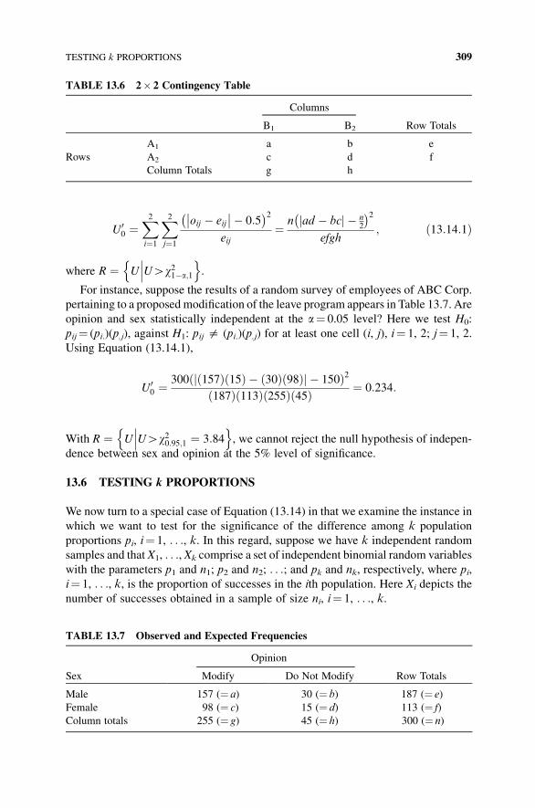
U00 ¼
X2
i¼1
X2
j¼1
oij � eij�� ��� 0:5� 2
eij¼ n ad � bcj j � n
2
� 2
efgh; ð13:14:1Þ
where R ¼ U UHw21�a;1
���on.
For instance, suppose the results of a random survey of employees of ABC Corp.
pertaining to a proposed modification of the leave program appears in Table 13.7. Are
opinion and sex statistically independent at the a¼ 0.05 level? Here we test H0:
pij¼ (pi.)(p.j), against H1: pij $ (pi.)(p.j) for at least one cell (i, j), i¼ 1, 2; j¼ 1, 2.
Using Equation (13.14.1),
U00 ¼
300ð ð157Þð15Þ � ð30Þð98Þj j � 150Þ2ð187Þð113Þð255Þð45Þ ¼ 0:234:
With R ¼ U UHw20:95;1 ¼ 3:84���
on, we cannot reject the null hypothesis of indepen-
dence between sex and opinion at the 5% level of significance.
13.6 TESTING k PROPORTIONS
We now turn to a special case of Equation (13.14) in that we examine the instance in
which we want to test for the significance of the difference among k population
proportions pi, i¼ 1, . . ., k. In this regard, suppose we have k independent random
samples and that X1, . . ., Xk comprise a set of independent binomial random variables
with the parameters p1 and n1; p2 and n2; . . .; and pk and nk, respectively, where pi,
i¼ 1, . . ., k, is the proportion of successes in the ith population. Here Xi depicts the
number of successes obtained in a sample of size ni, i¼ 1, . . ., k.
TABLE 13.6 2� 2 Contingency Table
Columns
B1 B2 Row Totals
A1 a b e
Rows A2 c d f
Column Totals g h
TABLE 13.7 Observed and Expected Frequencies
Opinion
Sex Modify Do Not Modify Row Totals
Male 157 (¼ a) 30 (¼ b) 187 (¼ e)
Female 98 (¼ c) 15 (¼ d) 113 (¼ f)
Column totals 255 (¼ g) 45 (¼ h) 300 (¼ n)
TESTING k PROPORTIONS 309
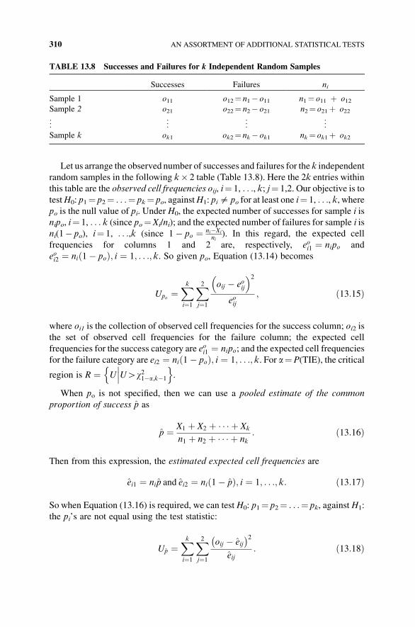
Let us arrange the observed number of successes and failures for the k independent
random samples in the following k� 2 table (Table 13.8). Here the 2k entries within
this table are the observed cell frequencies oij, i¼ 1, . . ., k; j¼ 1,2. Our objective is to
testH0: p1¼ p2¼ . . .¼ pk¼ po, againstH1: pi$ po for at least one i¼ 1, . . ., k, wherepo is the null value of pi. Under H0, the expected number of successes for sample i is
nipo, i¼ 1, . . . k (since po¼Xi/ni); and the expected number of failures for sample i is
ni(1� po), i¼ 1, . . .,k (since 1� po ¼ ni�Xi
ni). In this regard, the expected cell
frequencies for columns 1 and 2 are, respectively, eoi1 ¼ nipo and
eoi2 ¼ nið1� poÞ; i ¼ 1; . . .; k. So given po, Equation (13.14) becomes
Upo ¼Xk
i¼1
X2
j¼1
oij � eoij
� �2
eoij; ð13:15Þ
where oi1 is the collection of observed cell frequencies for the success column; oi2 is
the set of observed cell frequencies for the failure column; the expected cell
frequencies for the success category are eoi1 ¼ nipo; and the expected cell frequencies
for the failure category are ei2 ¼ ni 1� poð Þ; i ¼ 1; . . .; k. For a¼P(TIE), the critical
region is R ¼ U UHw21�a;k�1
���on.
When po is not specified, then we can use a pooled estimate of the common
proportion of success p as
p ¼ X1 þ X2 þ � � � þ Xk
n1 þ n2 þ � � � þ nk: ð13:16Þ
Then from this expression, the estimated expected cell frequencies are
ei1 ¼ nip and ei2 ¼ ni 1� pð Þ; i ¼ 1; . . .; k: ð13:17Þ
So when Equation (13.16) is required, we can test H0: p1¼ p2¼ . . .¼ pk, against H1:
the pi’s are not equal using the test statistic:
Up ¼Xk
i¼1
X2
j¼1
oij � eij� �2
eij: ð13:18Þ
TABLE 13.8 Successes and Failures for k Independent Random Samples
Successes Failures ni
Sample 1 o11 o12¼ n1� o11 n1¼ o11 þ o12Sample 2 o21 o22¼ n2� o21 n2¼ o21þ o22
..
. ... ..
. ...
Sample k ok1 ok2¼ nk� ok1 nk¼ ok1þ ok2
310 AN ASSORTMENT OF ADDITIONAL STATISTICAL TESTS
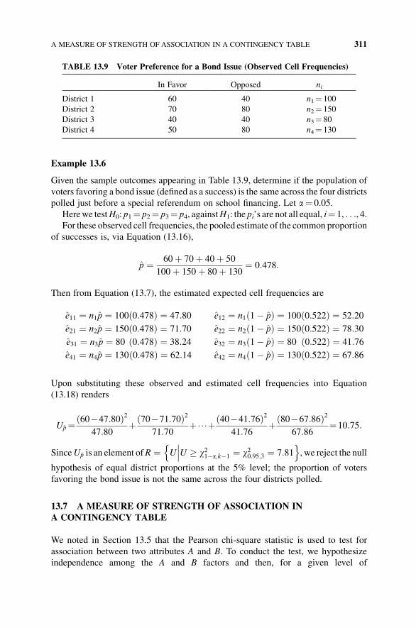
Example 13.6
Given the sample outcomes appearing in Table 13.9, determine if the population of
voters favoring a bond issue (defined as a success) is the same across the four districts
polled just before a special referendum on school financing. Let a¼ 0.05.
Herewe testH0: p1¼ p2¼ p3¼ p4, againstH1: the pi’s are not all equal, i¼ 1, . . ., 4.For these observed cell frequencies, the pooled estimate of the common proportion
of successes is, via Equation (13.16),
p ¼ 60þ 70þ 40þ 50
100þ 150þ 80þ 130¼ 0:478:
Then from Equation (13.7), the estimated expected cell frequencies are
e11 ¼ n1p ¼ 100ð0:478Þ ¼ 47:80
e21 ¼ n2p ¼ 150ð0:478Þ ¼ 71:70
e31 ¼ n3p ¼ 80 ð0:478Þ ¼ 38:24
e41 ¼ n4p ¼ 130ð0:478Þ ¼ 62:14
e12 ¼ n1ð1� pÞ ¼ 100ð0:522Þ ¼ 52:20
e22 ¼ n2ð1� pÞ ¼ 150ð0:522Þ ¼ 78:30
e32 ¼ n3ð1� pÞ ¼ 80 ð0:522Þ ¼ 41:76
e42 ¼ n4ð1� pÞ ¼ 130ð0:522Þ ¼ 67:86
Upon substituting these observed and estimated cell frequencies into Equation
(13.18) renders
Up¼ 60�47:80ð Þ247:80
þ 70�71:70ð Þ271:70
þ���þ 40�41:76ð Þ241:76
þ 80�67:86ð Þ267:86
¼10:75:
SinceUp is an element ofR ¼ U U � w21�a;k�1 ¼ w20:95;3 ¼ 7:81���
on, we reject the null
hypothesis of equal district proportions at the 5% level; the proportion of voters
favoring the bond issue is not the same across the four districts polled.
13.7 A MEASURE OF STRENGTH OF ASSOCIATION IN
A CONTINGENCY TABLE
We noted in Section 13.5 that the Pearson chi-square statistic is used to test for
association between two attributes A and B. To conduct the test, we hypothesize
independence among the A and B factors and then, for a given level of
TABLE 13.9 Voter Preference for a Bond Issue (Observed Cell Frequencies)
In Favor Opposed ni
District 1 60 40 n1¼ 100
District 2 70 80 n2¼ 150
District 3 40 40 n3¼ 80
District 4 50 80 n4¼ 130
A MEASURE OF STRENGTH OF ASSOCIATION IN A CONTINGENCY TABLE 311
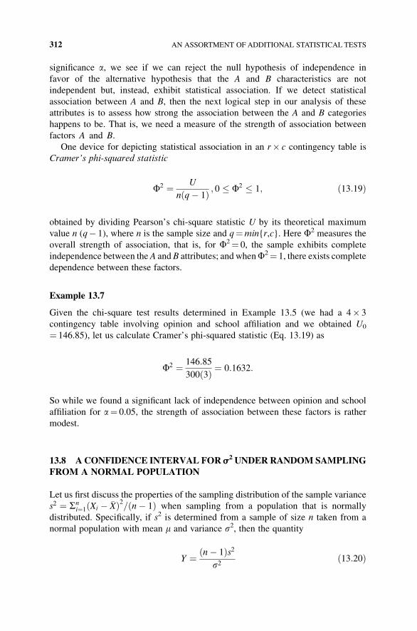
significance a, we see if we can reject the null hypothesis of independence in
favor of the alternative hypothesis that the A and B characteristics are not
independent but, instead, exhibit statistical association. If we detect statistical
association between A and B, then the next logical step in our analysis of these
attributes is to assess how strong the association between the A and B categories
happens to be. That is, we need a measure of the strength of association between
factors A and B.
One device for depicting statistical association in an r� c contingency table is
Cramer’s phi-squared statistic
F2 ¼ U
nðq� 1Þ ; 0 � F2 � 1; ð13:19Þ
obtained by dividing Pearson’s chi-square statistic U by its theoretical maximum
value n (q� 1), where n is the sample size and q¼min{r,c}. Here F2 measures the
overall strength of association, that is, for F2¼ 0, the sample exhibits complete
independence between the A and B attributes; and whenF2¼ 1, there exists complete
dependence between these factors.
Example 13.7
Given the chi-square test results determined in Example 13.5 (we had a 4� 3
contingency table involving opinion and school affiliation and we obtained U0
¼ 146.85), let us calculate Cramer’s phi-squared statistic (Eq. 13.19) as
F2 ¼ 146:85
300ð3Þ ¼ 0:1632:
So while we found a significant lack of independence between opinion and school
affiliation for a¼ 0.05, the strength of association between these factors is rather
modest.
13.8 A CONFIDENCE INTERVAL FOR s2 UNDER RANDOM SAMPLING
FROM A NORMAL POPULATION
Let us first discuss the properties of the sampling distribution of the sample variance
s2 ¼ Sni¼1 Xi � �Xð Þ2= n� 1ð Þ when sampling from a population that is normally
distributed. Specifically, if s2 is determined from a sample of size n taken from a
normal population with mean m and variance s2, then the quantity
Y ¼ n� 1ð Þs2s2
ð13:20Þ
312 AN ASSORTMENT OF ADDITIONAL STATISTICAL TESTS
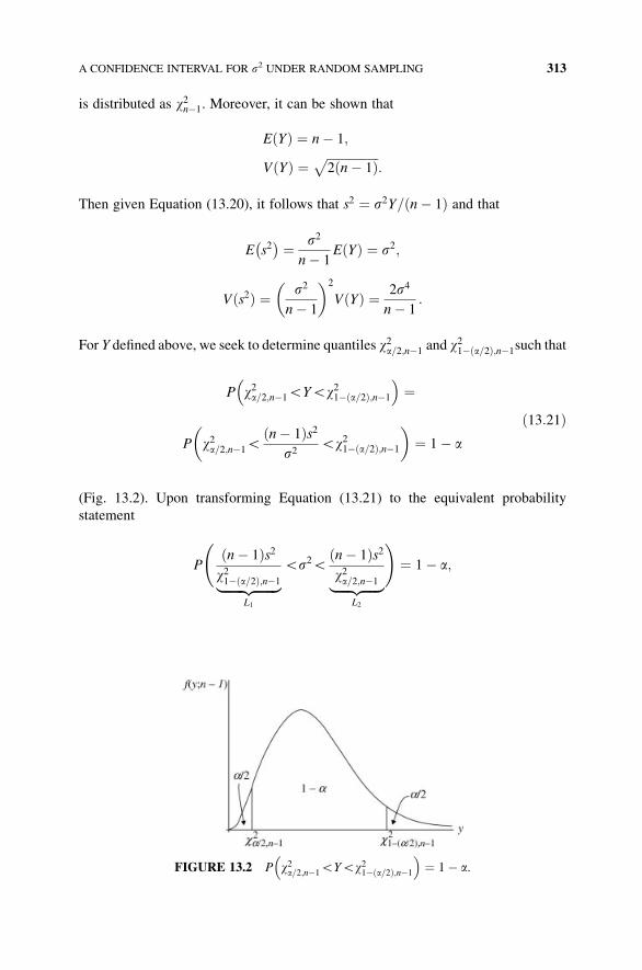
is distributed as w2n�1. Moreover, it can be shown that
EðYÞ ¼ n� 1;
VðYÞ ¼ ffiffiffiffiffiffiffiffiffiffiffiffiffiffiffiffiffi2ðn� 1Þp
:
Then given Equation (13.20), it follows that s2 ¼ s2Y=ðn� 1Þ and that
E s2� ¼ s2
n� 1EðYÞ ¼ s2;
Vðs2Þ ¼ s2
n� 1
� �2
VðYÞ ¼ 2s4
n� 1:
For Y defined above, we seek to determine quantiles w2a=2;n�1 and w21�ða=2Þ;n�1such that
P w2a=2;n�1GYGw21�ða=2Þ;n�1
� �¼
P w2a=2;n�1Gn� 1ð Þs2
s2Gw21� a=2ð Þ;n�1
� �¼ 1� a
ð13:21Þ
(Fig. 13.2). Upon transforming Equation (13.21) to the equivalent probability
statement
P
ðn� 1Þs2w21�ða=2Þ;n�1|fflfflfflfflfflfflffl{zfflfflfflfflfflfflffl}
L1
Gs2Gðn� 1Þs2w2a=2;n�1|fflfflfflfflffl{zfflfflfflfflffl}
L2
!¼ 1� a;
FIGURE 13.2 P w2a=2;n�1GYGw21�ða=2Þ;n�1
� �¼ 1� a.
A CONFIDENCE INTERVAL FOR s2 UNDER RANDOM SAMPLING 313
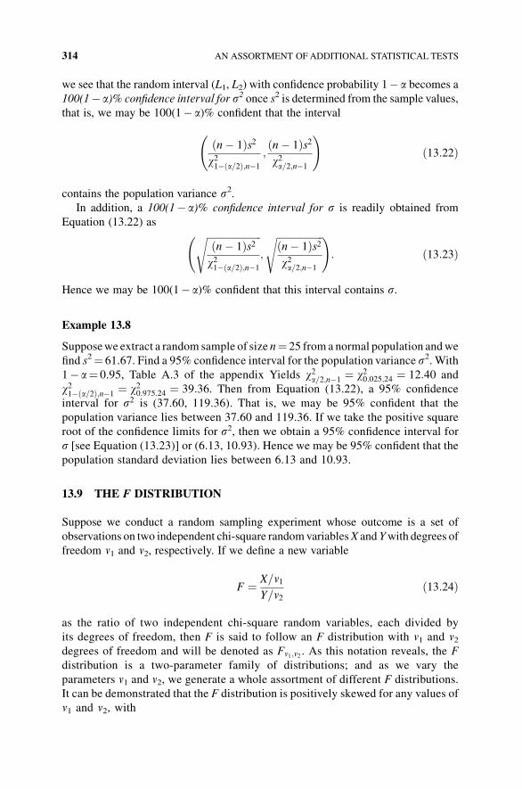
we see that the random interval (L1, L2) with confidence probability 1� a becomes a
100(1� a)% confidence interval for s2 once s2 is determined from the sample values,
that is, we may be 100(1� a)% confident that the interval
ðn� 1Þs2w21�ða=2Þ;n�1
;ðn� 1Þs2w2a=2;n�1
!ð13:22Þ
contains the population variance s2.In addition, a 100(1� a)% confidence interval for s is readily obtained from
Equation (13.22) asffiffiffiffiffiffiffiffiffiffiffiffiffiffiffiffiffiffiffiffiffiffiðn� 1Þs2w21�ða=2Þ;n�1
s;
ffiffiffiffiffiffiffiffiffiffiffiffiffiffiffiffiffiffiffiðn� 1Þs2w2a=2;n�1
s !: ð13:23Þ
Hence we may be 100(1� a)% confident that this interval contains s.
Example 13.8
Supposewe extract a random sample of size n¼ 25 from a normal population andwe
find s2¼ 61.67. Find a 95% confidence interval for the population variance s2. With
1� a¼ 0.95, Table A.3 of the appendix Yields w2a=2;n�1 ¼ w20:025;24 ¼ 12:40 and
w21�ða=2Þ;n�1 ¼ w20:975:24 ¼ 39:36. Then from Equation (13.22), a 95% confidence
interval for s2 is (37.60, 119.36). That is, we may be 95% confident that the
population variance lies between 37.60 and 119.36. If we take the positive square
root of the confidence limits for s2, then we obtain a 95% confidence interval for
s [see Equation (13.23)] or (6.13, 10.93). Hence we may be 95% confident that the
population standard deviation lies between 6.13 and 10.93.
13.9 THE F DISTRIBUTION
Suppose we conduct a random sampling experiment whose outcome is a set of
observations on two independent chi-square randomvariablesX and Ywith degrees of
freedom v1 and v2, respectively. If we define a new variable
F ¼ X=v1Y=v2
ð13:24Þ
as the ratio of two independent chi-square random variables, each divided by
its degrees of freedom, then F is said to follow an F distribution with v1 and v2degrees of freedom and will be denoted as Fv1;v2 . As this notation reveals, the F
distribution is a two-parameter family of distributions; and as we vary the
parameters v1 and v2, we generate a whole assortment of different F distributions.
It can be demonstrated that the F distribution is positively skewed for any values of
v1 and v2, with
314 AN ASSORTMENT OF ADDITIONAL STATISTICAL TESTS
E Fð Þ ¼ v2
v2 � 2; v2H2;
V Fð Þ ¼ 2v2 v1 þ v2 � 2ð Þv1 v2 � 2ð Þ2 v2 � 4ð Þ ; v2H4:
Moreover, unlike the t or Z distributions, the F distribution can only assume positive
values.
What is the connection between Equation (13.24) and sampling from a normal
population? Suppose a random sample of size n1 with variance s21 is drawn from a
N(m1,s1) population and a second random sample size n2 with variance s22 is extracted
from a population which is N(m2,s2). If these two random samples are independent,
then, via Equation (13.20), X¼ (n1� 1)s21/s21 and Y¼ (n2� 1)s22=s
22 are independent
chi-square random variables with v1¼ n1� 1 and v2¼ n2� 1 degrees of freedom,
respectively. Then from Equation (13.24), the random variable
Fn1�1;n2�1 ¼ s21=s21
s22=s22
ð13:25Þ
is F distributed with n1� 1 and n2� 1 degrees of freedom.
How do we obtain the percentage points or quantiles of the F distribution? The
upper tail a percentage pointF a;v1;v2 for F appears in Table A.4 of the appendix and is
defined by
P F � Fa;v1;v2
� ¼ a ð13:26Þ(Fig. 13.3). Only the upper tail a percentage points are given since the lower tail 1� apercentage point F1�a;v1;v2 for F is the reciprocal of the upper tail a percentage pointwith degrees of freedom reversed or
F1�a;v1;v2 ¼1
Fa;v2;v1: ð13:27Þ
FIGURE 13.3 The Fa;v1 ;v2distribution.
THE F DISTRIBUTION 315
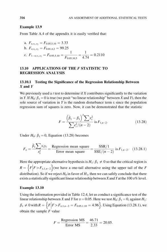
Example 13.9
From Table A.4 of the appendix it is easily verified that:
a. Fa;v1;v2 ¼ F0:05;5;10 ¼ 3:33
b. Fa;v1;v2 ¼ F0:01;4;2 ¼ 99:25
c. F1�a;v1;v2 ¼ F0:95;5;10 ¼ 1
F0:05;10;5¼ 1
4:74¼ 0:2110
13.10 APPLICATIONS OF THE F STATISTIC TO
REGRESSION ANALYSIS
13.10.1 Testing the Significance of the Regression Relationship Between
X and Y
We previously used a t test to determine if X contributes significantly to the variation
in Y. IfH0: b1¼ 0 is true (we posit “no linear relationship” between X and Y), then the
sole source of variation in Y is the random disturbance term e since the populationregression sum of squares is zero. Now, it can be demonstrated that the statistic
F ¼b1 � b1� �2X
x2iXe2i =ðn� 2Þ is F1;n�2: ð13:28Þ
Under H0: b1¼ 0, Equation (13.28) becomes
Fo ¼b1X
xiyi
s2e¼ Regression mean square
Error mean square¼ SSR=1
SSE= n� 2ð Þ is F1;n�2: ð13:28:1Þ
Here the appropriate alternative hypothesis is H1: b1$ 0 so that the critical region is
R ¼ F FHFa;1;n�2
���on(we have a one-tail alternative using the upper tail of the F
distribution). So if we rejectH0 in favor ofH1, then we can safely conclude that there
exists a statistically significant linear relationship betweenX andY at the 100 a%level.
Example 13.10
Using the information provided in Table 12.4, let us conduct a significance test of the
linear relationship between X and Y for a¼ 0.05. Here we testH0: b1¼ 0, againstH1:
b1$ 0withR ¼ F FHFa;1;n�2 ¼ F0:05;1;10 ¼ 4:96���
on. Using Equation (13.28.1), we
obtain the sample F value
F ¼ Regression MS
Error MS¼ 46:71
2:33¼ 20:05:
316 AN ASSORTMENT OF ADDITIONAL STATISTICAL TESTS
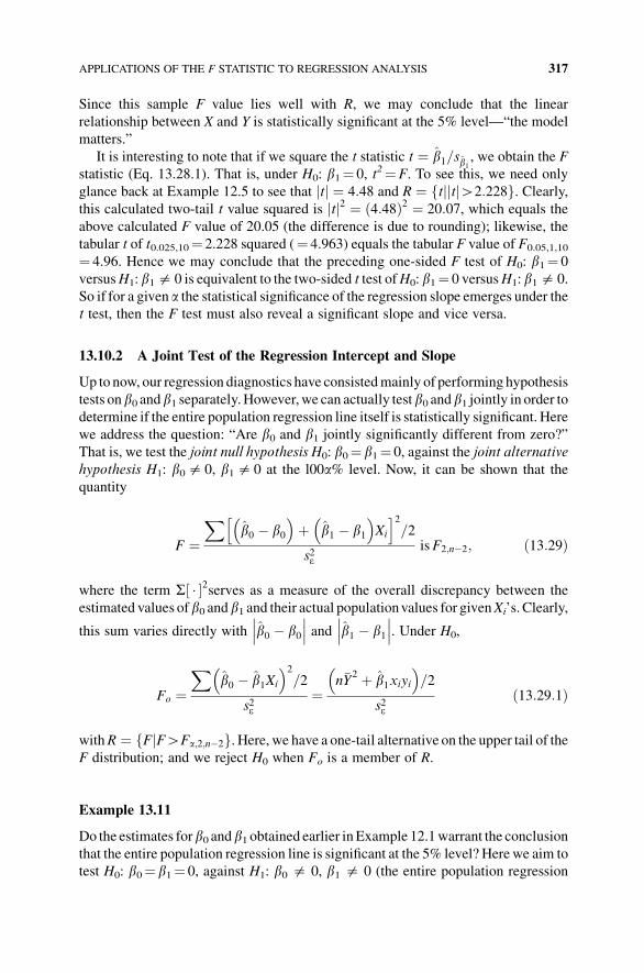
Since this sample F value lies well with R, we may conclude that the linear
relationship between X and Y is statistically significant at the 5% level—“the model
matters.”
It is interesting to note that if we square the t statistic t ¼ b1=sb1 , we obtain the Fstatistic (Eq. 13.28.1). That is, under H0: b1¼ 0, t2¼F. To see this, we need only
glance back at Example 12.5 to see that tj j ¼ 4:48 and R ¼ tjjtf jH2:228g. Clearly,this calculated two-tail t value squared is tj j2 ¼ 4:48ð Þ2 ¼ 20:07, which equals the
above calculated F value of 20.05 (the difference is due to rounding); likewise, the
tabular t of t0.025,10¼ 2.228 squared (¼ 4.963) equals the tabular F value of F0.05,1,10
¼ 4.96. Hence we may conclude that the preceding one-sided F test of H0: b1¼ 0
versusH1: b1$ 0 is equivalent to the two-sided t test ofH0: b1¼ 0 versusH1: b1$ 0.
So if for a given a the statistical significance of the regression slope emerges under the
t test, then the F test must also reveal a significant slope and vice versa.
13.10.2 A Joint Test of the Regression Intercept and Slope
Up to now, our regression diagnostics have consistedmainly of performing hypothesis
tests onb0 andb1 separately.However,we can actually testb0 andb1 jointly in order todetermine if the entire population regression line itself is statistically significant. Here
we address the question: “Are b0 and b1 jointly significantly different from zero?”
That is, we test the joint null hypothesis H0: b0¼ b1¼ 0, against the joint alternative
hypothesis H1: b0$ 0, b1$ 0 at the l00a% level. Now, it can be shown that the
quantity
F ¼X
b0 � b0� �
þ b1 � b1� �
Xi
h i2=2
s2eisF2;n�2; ð13:29Þ
where the term S �½ �2serves as a measure of the overall discrepancy between the
estimated values ofb0 andb1 and their actual populationvalues for givenXi’s. Clearly,
this sum varies directly with b0 � b0���
��� and b1 � b1���
���. Under H0,
Fo ¼X
b0 � b1Xi
� �2=2
s2e¼
n�Y2 þ b1xiyi
� �=2
s2eð13:29:1Þ
withR ¼ Ff jFHFa;2;n�2g. Here, we have a one-tail alternative on the upper tail of theF distribution; and we reject H0 when Fo is a member of R.
Example 13.11
Do the estimates forb0 andb1 obtained earlier inExample 12.1warrant the conclusion
that the entire population regression line is significant at the 5% level? Herewe aim to
test H0: b0¼ b1¼ 0, against H1: b0 $ 0, b1 $ 0 (the entire population regression
APPLICATIONS OF THE F STATISTIC TO REGRESSION ANALYSIS 317
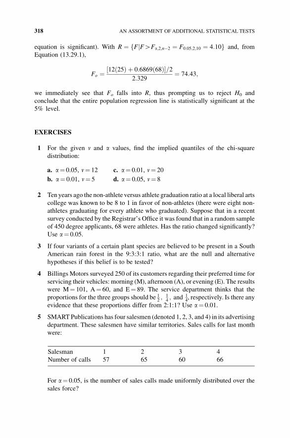
equation is significant). With R ¼ Ff jFHFa;2;n�2 ¼ F0:05;2;10 ¼ 4:10g and, from
Equation (13.29.1),
Fo ¼ 12ð25Þ þ 0:6869ð68Þ½ �=22:329
¼ 74:43;
we immediately see that Fo falls into R, thus prompting us to reject H0 and
conclude that the entire population regression line is statistically significant at the
5% level.
EXERCISES
1 For the given v and a values, find the implied quantiles of the chi-square
distribution:
a. a¼ 0.05, v¼ 12
b. a¼ 0.01, v¼ 5
c. a¼ 0.01, v¼ 20
d. a¼ 0.05, v¼ 8
2 Ten years ago the non-athlete versus athlete graduation ratio at a local liberal arts
college was known to be 8 to 1 in favor of non-athletes (there were eight non-
athletes graduating for every athlete who graduated). Suppose that in a recent
survey conducted by the Registrar’s Office it was found that in a random sample
of 450 degree applicants, 68 were athletes. Has the ratio changed significantly?
Use a¼ 0.05.
3 If four variants of a certain plant species are believed to be present in a South
American rain forest in the 9:3:3:1 ratio, what are the null and alternative
hypotheses if this belief is to be tested?
4 Billings Motors surveyed 250 of its customers regarding their preferred time for
servicing their vehicles: morning (M), afternoon (A), or evening (E). The results
were M¼ 101, A¼ 60, and E¼ 89. The service department thinks that the
proportions for the three groups should be 12; 1
4; and 1
4, respectively. Is there any
evidence that these proportions differ from 2:1:1? Use a¼ 0.01.
5 SMART Publications has four salesmen (denoted 1, 2, 3, and 4) in its advertising
department. These salesmen have similar territories. Sales calls for last month
were:
Salesman 1 2 3 4
Number of calls 57 65 60 66
For a¼ 0.05, is the number of sales calls made uniformly distributed over the
sales force?
318 AN ASSORTMENT OF ADDITIONAL STATISTICAL TESTS
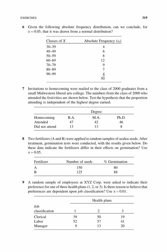
6 Given the following absolute frequency distribution, can we conclude, for
a¼ 0.05, that it was drawn from a normal distribution?
Classes of X Absolute Frequency (oi)
30–39 4
40–49 6
50–59 8
60–69 12
70–79 9
80–89 7
90–99 4
50
7 Invitations to homecoming were mailed to the class of 2000 graduates from a
small Midwestern liberal arts college. The numbers from the class of 2000 who
attended the festivities are shown below. Test the hypothesis that the proportion
attending is independent of the highest degree earned.
Degree
Homecoming B.A. M.A. Ph.D.
Attended 47 42 46
Did not attend 13 13 8
8 Two fertilizers (A and B) were applied to random samples of azalea seeds. After
treatment, germination tests were conducted, with the results given below. Do
these data indicate the fertilizers differ in their effects on germination? Use
a¼ 0.05.
Fertilizer Number of seeds % Germination
A 150 80
B 125 88
9 A random sample of employees at XYZ Corp. were asked to indicate their
preference for one of three health plans (1, 2, or 3). Is there reason to believe that
preferences are dependent upon job classification? Use a¼ 0.01.
Health plans
Job
classification 1 2 3
Clerical 39 50 19
Labor 52 57 41
Manager 9 13 20
EXERCISES 319
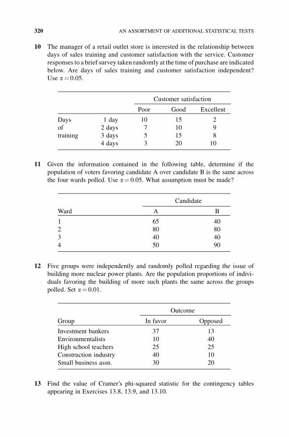
10 The manager of a retail outlet store is interested in the relationship between
days of sales training and customer satisfaction with the service. Customer
responses to a brief survey taken randomly at the time of purchase are indicated
below. Are days of sales training and customer satisfaction independent?
Use a¼ 0.05.
Customer satisfaction
Poor Good Excellent
Days 1 day 10 15 2
of 2 days 7 10 9
training 3 days 5 15 8
4 days 3 20 10
11 Given the information contained in the following table, determine if the
population of voters favoring candidate A over candidate B is the same across
the four wards polled. Use a¼ 0.05. What assumption must be made?
Candidate
Ward A B
1 65 40
2 80 80
3 40 40
4 50 90
12 Five groups were independently and randomly polled regarding the issue of
building more nuclear power plants. Are the population proportions of indivi-
duals favoring the building of more such plants the same across the groups
polled. Set a¼ 0.01.
Outcome
Group In favor Opposed
Investment bankers 37 13
Environmentalists 10 40
High school teachers 25 25
Construction industry 40 10
Small business assn. 30 20
13 Find the value of Cramer’s phi-squared statistic for the contingency tables
appearing in Exercises 13.8, 13.9, and 13.10.
320 AN ASSORTMENT OF ADDITIONAL STATISTICAL TESTS
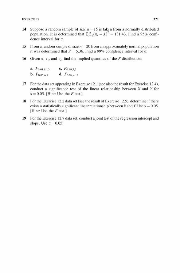
14 Suppose a random sample of size n¼ 15 is taken from a normally distributed
population. It is determined that S15i¼1 Xi � �Xð Þ2 ¼ 131:43. Find a 95% confi-
dence interval for s.
15 From a random sample of size n¼ 20 from an approximately normal population
it was determined that s2¼ 5.36. Find a 99% confidence interval for s.
16 Given a, v1, and v2, find the implied quantiles of the F distribution:
a. F0.01,8,10
b. F0.05,6,9
c. F0.99,7,5
d. F0.99,4,12
17 For the data set appearing in Exercise 12.1 (see also the result for Exercise 12.4),
conduct a significance test of the linear relationship between X and Y for
a¼ 0.05. [Hint: Use the F test.]
18 For the Exercise 12.2 data set (see the result of Exercise 12.5), determine if there
exists a statistically significant linear relationship betweenX andY. Use a¼ 0.05.
[Hint: Use the F test.]
19 For the Exercise 12.7 data set, conduct a joint test of the regression intercept and
slope. Use a¼ 0.05.
EXERCISES 321
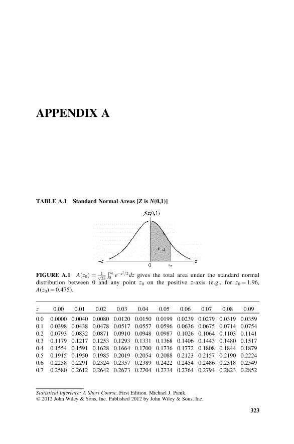
APPENDIX A
TABLE A.1 Standard Normal Areas [Z is N(0,1)]
z 0.00 0.01 0.02 0.03 0.04 0.05 0.06 0.07 0.08 0.09
0.0 0.0000 0.0040 0.0080 0.0120 0.0150 0.0199 0.0239 0.0279 0.0319 0.0359
0.1 0.0398 0.0438 0.0478 0.0517 0.0557 0.0596 0.0636 0.0675 0.0714 0.0754
0.2 0.0793 0.0832 0.0871 0.0910 0.0948 0.0987 0.1026 0.1064 0.1103 0.1141
0.3 0.1179 0.1217 0.1253 0.1293 0.1331 0.1368 0.1406 0.1443 0.1480 0.1517
0.4 0.1554 0.1591 0.1628 0.1664 0.1700 0.1736 0.1772 0.1808 0.1844 0.1879
0.5 0.1915 0.1950 0.1985 0.2019 0.2054 0.2088 0.2123 0.2157 0.2190 0.2224
0.6 0.2258 0.2291 0.2324 0.2357 0.2389 0.2422 0.2454 0.2486 0.2518 0.2549
0.7 0.2580 0.2612 0.2642 0.2673 0.2704 0.2734 0.2764 0.2794 0.2823 0.2852
FIGURE A.1 Aðz0Þ ¼ 1ffiffiffiffi2p
pÐ z00e�z2=2dz gives the total area under the standard normal
distribution between 0 and any point z0 on the positive z-axis (e.g., for z0¼ 1.96,
A(z0)¼ 0.475).
Statistical Inference: A Short Course, First Edition. Michael J. Panik.� 2012 John Wiley & Sons, Inc. Published 2012 by John Wiley & Sons, Inc.
323
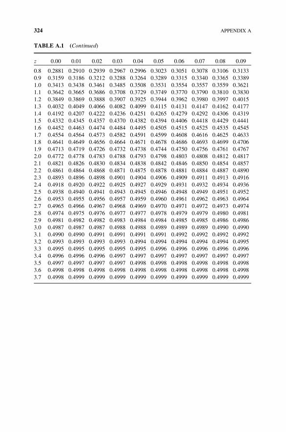
TABLE A.1 (Continued)
z 0.00 0.01 0.02 0.03 0.04 0.05 0.06 0.07 0.08 0.09
0.8 0.2881 0.2910 0.2939 0.2967 0.2996 0.3023 0.3051 0.3078 0.3106 0.3133
0.9 0.3159 0.3186 0.3212 0.3288 0.3264 0.3289 0.3315 0.3340 0.3365 0.3389
1.0 0.3413 0.3438 0.3461 0.3485 0.3508 0.3531 0.3554 0.3557 0.3559 0.3621
1.1 0.3642 0.3665 0.3686 0.3708 0.3729 0.3749 0.3770 0.3790 0.3810 0.3830
1.2 0.3849 0.3869 0.3888 0.3907 0.3925 0.3944 0.3962 0.3980 0.3997 0.4015
1.3 0.4032 0.4049 0.4066 0.4082 0.4099 0.4115 0.4131 0.4147 0.4162 0.4177
1.4 0.4192 0.4207 0.4222 0.4236 0.4251 0.4265 0.4279 0.4292 0.4306 0.4319
1.5 0.4332 0.4345 0.4357 0.4370 0.4382 0.4394 0.4406 0.4418 0.4429 0.4441
1.6 0.4452 0.4463 0.4474 0.4484 0.4495 0.4505 0.4515 0.4525 0.4535 0.4545
1.7 0.4554 0.4564 0.4573 0.4582 0.4591 0.4599 0.4608 0.4616 0.4625 0.4633
1.8 0.4641 0.4649 0.4656 0.4664 0.4671 0.4678 0.4686 0.4693 0.4699 0.4706
1.9 0.4713 0.4719 0.4726 0.4732 0.4738 0.4744 0.4750 0.4756 0.4761 0.4767
2.0 0.4772 0.4778 0.4783 0.4788 0.4793 0.4798 0.4803 0.4808 0.4812 0.4817
2.1 0.4821 0.4826 0.4830 0.4834 0.4838 0.4842 0.4846 0.4850 0.4854 0.4857
2.2 0.4861 0.4864 0.4868 0.4871 0.4875 0.4878 0.4881 0.4884 0.4887 0.4890
2.3 0.4893 0.4896 0.4898 0.4901 0.4904 0.4906 0.4909 0.4911 0.4913 0.4916
2.4 0.4918 0.4920 0.4922 0.4925 0.4927 0.4929 0.4931 0.4932 0.4934 0.4936
2.5 0.4938 0.4940 0.4941 0.4943 0.4945 0.4946 0.4948 0.4949 0.4951 0.4952
2.6 0.4953 0.4955 0.4956 0.4957 0.4959 0.4960 0.4961 0.4962 0.4963 0.4964
2.7 0.4965 0.4966 0.4967 0.4968 0.4969 0.4970 0.4971 0.4972 0.4973 0.4974
2.8 0.4974 0.4975 0.4976 0.4977 0.4977 0.4978 0.4979 0.4979 0.4980 0.4981
2.9 0.4981 0.4982 0.4982 0.4983 0.4984 0.4984 0.4985 0.4985 0.4986 0.4986
3.0 0.4987 0.4987 0.4987 0.4988 0.4988 0.4989 0.4989 0.4989 0.4990 0.4990
3.1 0.4990 0.4990 0.4991 0.4991 0.4991 0.4991 0.4992 0.4992 0.4992 0.4992
3.2 0.4993 0.4993 0.4993 0.4993 0.4994 0.4994 0.4994 0.4994 0.4994 0.4995
3.3 0.4995 0.4995 0.4995 0.4995 0.4995 0.4996 0.4996 0.4996 0.4996 0.4996
3.4 0.4996 0.4996 0.4996 0.4997 0.4997 0.4997 0.4997 0.4997 0.4997 0.4997
3.5 0.4997 0.4997 0.4997 0.4997 0.4998 0.4998 0.4998 0.4998 0.4998 0.4998
3.6 0.4998 0.4998 0.4998 0.4998 0.4998 0.4998 0.4998 0.4998 0.4998 0.4998
3.7 0.4998 0.4999 0.4999 0.4999 0.4999 0.4999 0.4999 0.4999 0.4999 0.4999
324 APPENDIX A
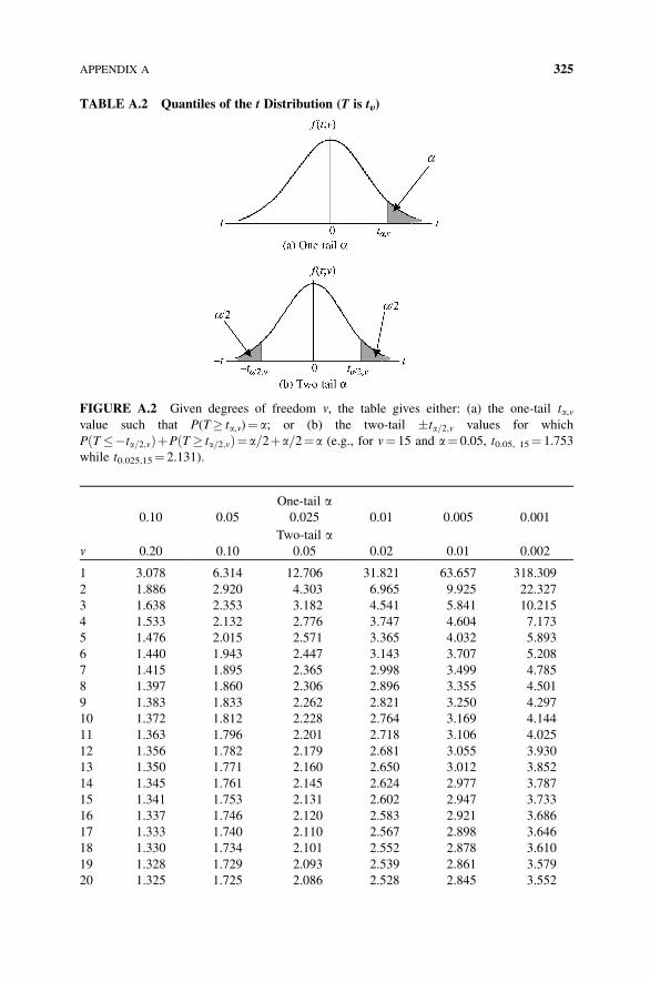
TABLE A.2 Quantiles of the t Distribution (T is tv)
0.10 0.05
One-tail a0.025 0.01 0.005 0.001
v 0.20 0.10
Two-tail a0.05 0.02 0.01 0.002
1 3.078 6.314 12.706 31.821 63.657 318.309
2 1.886 2.920 4.303 6.965 9.925 22.327
3 1.638 2.353 3.182 4.541 5.841 10.215
4 1.533 2.132 2.776 3.747 4.604 7.173
5 1.476 2.015 2.571 3.365 4.032 5.893
6 1.440 1.943 2.447 3.143 3.707 5.208
7 1.415 1.895 2.365 2.998 3.499 4.785
8 1.397 1.860 2.306 2.896 3.355 4.501
9 1.383 1.833 2.262 2.821 3.250 4.297
10 1.372 1.812 2.228 2.764 3.169 4.144
11 1.363 1.796 2.201 2.718 3.106 4.025
12 1.356 1.782 2.179 2.681 3.055 3.930
13 1.350 1.771 2.160 2.650 3.012 3.852
14 1.345 1.761 2.145 2.624 2.977 3.787
15 1.341 1.753 2.131 2.602 2.947 3.733
16 1.337 1.746 2.120 2.583 2.921 3.686
17 1.333 1.740 2.110 2.567 2.898 3.646
18 1.330 1.734 2.101 2.552 2.878 3.610
19 1.328 1.729 2.093 2.539 2.861 3.579
20 1.325 1.725 2.086 2.528 2.845 3.552
FIGURE A.2 Given degrees of freedom v, the table gives either: (a) the one-tail ta,vvalue such that P(T� ta,v)¼ a; or (b) the two-tail �ta=2;v values for which
PðT��ta=2;vÞþPðT� ta=2;vÞ¼a=2þa=2¼a (e.g., for v¼ 15 and a¼ 0.05, t0.05, 15¼ 1.753
while t0.025,15¼ 2.131).
APPENDIX A 325
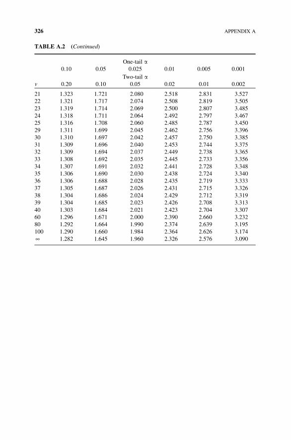
TABLE A.2 (Continued)
0.10 0.05
One-tail a0.025 0.01 0.005 0.001
v 0.20 0.10
Two-tail a0.05 0.02 0.01 0.002
21 1.323 1.721 2.080 2.518 2.831 3.527
22 1.321 1.717 2.074 2.508 2.819 3.505
23 1.319 1.714 2.069 2.500 2.807 3.485
24 1.318 1.711 2.064 2.492 2.797 3.467
25 1.316 1.708 2.060 2.485 2.787 3.450
29 1.311 1.699 2.045 2.462 2.756 3.396
30 1.310 1.697 2.042 2.457 2.750 3.385
31 1.309 1.696 2.040 2.453 2.744 3.375
32 1.309 1.694 2.037 2.449 2.738 3.365
33 1.308 1.692 2.035 2.445 2.733 3.356
34 1.307 1.691 2.032 2.441 2.728 3.348
35 1.306 1.690 2.030 2.438 2.724 3.340
36 1.306 1.688 2.028 2.435 2.719 3.333
37 1.305 1.687 2.026 2.431 2.715 3.326
38 1.304 1.686 2.024 2.429 2.712 3.319
39 1.304 1.685 2.023 2.426 2.708 3.313
40 1.303 1.684 2.021 2.423 2.704 3.307
60 1.296 1.671 2.000 2.390 2.660 3.232
80 1.292 1.664 1.990 2.374 2.639 3.195
100 1.290 1.660 1.984 2.364 2.626 3.174
¥ 1.282 1.645 1.960 2.326 2.576 3.090
326 APPENDIX A
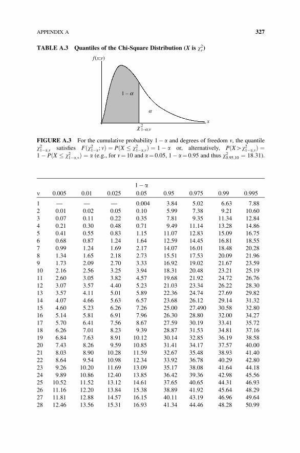
TABLE A.3 Quantiles of the Chi-Square Distribution (X is w2v)
1� an 0.005 0.01 0.025 0.05 0.95 0.975 0.99 0.995
1 — — — 0.004 3.84 5.02 6.63 7.88
2 0.01 0.02 0.05 0.10 5.99 7.38 9.21 10.60
3 0.07 0.11 0.22 0.35 7.81 9.35 11.34 12.84
4 0.21 0.30 0.48 0.71 9.49 11.14 13.28 14.86
5 0.41 0.55 0.83 1.15 11.07 12.83 15.09 16.75
6 0.68 0.87 1.24 1.64 12.59 14.45 16.81 18.55
7 0.99 1.24 1.69 2.17 14.07 16.01 18.48 20.28
8 1.34 1.65 2.18 2.73 15.51 17.53 20.09 21.96
9 1.73 2.09 2.70 3.33 16.92 19.02 21.67 23.59
10 2.16 2.56 3.25 3.94 18.31 20.48 23.21 25.19
11 2.60 3.05 3.82 4.57 19.68 21.92 24.72 26.76
12 3.07 3.57 4.40 5.23 21.03 23.34 26.22 28.30
13 3.57 4.11 5.01 5.89 22.36 24.74 27.69 29.82
14 4.07 4.66 5.63 6.57 23.68 26.12 29.14 31.32
15 4.60 5.23 6.26 7.26 25.00 27.490 30.58 32.80
16 5.14 5.81 6.91 7.96 26.30 28.80 32.00 34.27
17 5.70 6.41 7.56 8.67 27.59 30.19 33.41 35.72
18 6.26 7.01 8.23 9.39 28.87 31.53 34.81 37.16
19 6.84 7.63 8.91 10.12 30.14 32.85 36.19 38.58
20 7.43 8.26 9.59 10.85 31.41 34.17 37.57 40.00
21 8.03 8.90 10.28 11.59 32.67 35.48 38.93 41.40
22 8.64 9.54 10.98 12.34 33.92 36.78 40.29 42.80
23 9.26 10.20 11.69 13.09 35.17 38.08 41.64 44.18
24 9.89 10.86 12.40 13.85 36.42 39.36 42.98 45.56
25 10.52 11.52 13.12 14.61 37.65 40.65 44.31 46.93
26 11.16 12.20 13.84 15.38 38.89 41.92 45.64 48.29
27 11.81 12.88 14.57 16.15 40.11 43.19 46.96 49.64
28 12.46 13.56 15.31 16.93 41.34 44.46 48.28 50.99
f(x;v)
1 – α
2x
α
χ 1–α,ν
FIGURE A.3 For the cumulative probability 1� a and degrees of freedom v, the quantile
w21�a;v satisfies Fðw21�a; nÞ ¼ PðX � w21�a;nÞ ¼ 1� a or, alternatively, PðXHw21�a;vÞ ¼1� PðX � w21�a;nÞ ¼ a (e.g., for v¼ 10 and a¼ 0.05, 1� a¼ 0.95 and thus w20:95;10 ¼ 18:31).
APPENDIX A 327
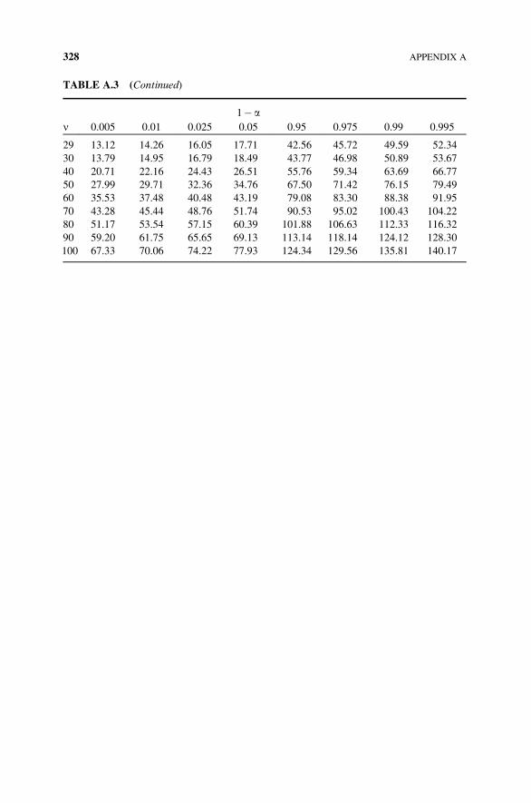
TABLE A.3 (Continued)
1� an 0.005 0.01 0.025 0.05 0.95 0.975 0.99 0.995
29 13.12 14.26 16.05 17.71 42.56 45.72 49.59 52.34
30 13.79 14.95 16.79 18.49 43.77 46.98 50.89 53.67
40 20.71 22.16 24.43 26.51 55.76 59.34 63.69 66.77
50 27.99 29.71 32.36 34.76 67.50 71.42 76.15 79.49
60 35.53 37.48 40.48 43.19 79.08 83.30 88.38 91.95
70 43.28 45.44 48.76 51.74 90.53 95.02 100.43 104.22
80 51.17 53.54 57.15 60.39 101.88 106.63 112.33 116.32
90 59.20 61.75 65.65 69.13 113.14 118.14 124.12 128.30
100 67.33 70.06 74.22 77.93 124.34 129.56 135.81 140.17
328 APPENDIX A
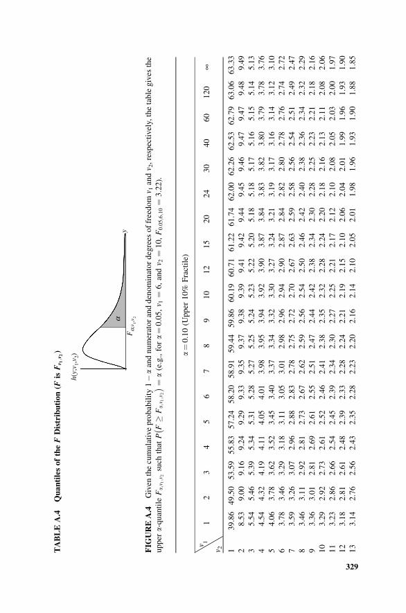
TABLEA.4
QuantilesoftheFDistribution(F
isFv 1;v2) a¼0.10(U
pper
10%
Fractile)
v 11
23
45
67
89
10
12
15
20
24
30
40
60
120
¥v 2 1
39.86
49.50
53.59
55.83
57.24
58.20
58.91
59.44
59.86
60.19
60.71
61.22
61.74
62.00
62.26
62.53
62.79
63.06
63.33
28.53
9.00
9.16
9.24
9.29
9.33
9.35
9.37
9.38
9.39
9.41
9.42
9.44
9.45
9.46
9.47
9.47
9.48
9.49
35.54
5.46
5.39
5.34
5.31
5.28
5.27
5.25
5.24
5.23
5.22
5.20
5.18
5.18
5.17
5.16
5.15
5.14
5.13
44.54
4.32
4.19
4.11
4.05
4.01
3.98
3.95
3.94
3.92
3.90
3.87
3.84
3.83
3.82
3.80
3.79
3.78
3.76
54.06
3.78
3.62
3.52
3.45
3.40
3.37
3.34
3.32
3.30
3.27
3.24
3.21
3.19
3.17
3.16
3.14
3.12
3.10
63.78
3.46
3.29
3.18
3.11
3.05
3.01
2.98
2.96
2.94
2.90
2.87
2.84
2.82
2.80
2.78
2.76
2.74
2.72
73.59
3.26
3.07
2.96
2.88
2.83
2.78
2.75
2.72
2.70
2.67
2.63
2.59
2.58
2.56
2.54
2.51
2.49
2.47
83.46
3.11
2.92
2.81
2.73
2.67
2.62
2.59
2.56
2.54
2.50
2.46
2.42
2.40
2.38
2.36
2.34
2.32
2.29
93.36
3.01
2.81
2.69
2.61
2.55
2.51
2.47
2.44
2.42
2.38
2.34
2.30
2.28
2.25
2.23
2.21
2.18
2.16
10
3.29
2.92
2.73
2.61
2.52
2.46
2.41
2.38
2.35
2.32
2.28
2.24
2.20
2.18
2.16
2.13
2.11
2.08
2.06
11
3.23
2.86
2.66
2.54
2.45
2.39
2.34
2.30
2.27
2.25
2.21
2.17
2.12
2.10
2.08
2.05
2.03
2.00
1.97
12
3.18
2.81
2.61
2.48
2.39
2.33
2.28
2.24
2.21
2.19
2.15
2.10
2.06
2.04
2.01
1.99
1.96
1.93
1.90
13
3.14
2.76
2.56
2.43
2.35
2.28
2.23
2.20
2.16
2.14
2.10
2.05
2.01
1.98
1.96
1.93
1.90
1.88
1.85
h(y;
v 1,v
2)
Fα,
v 1,v 2α
y
FIG
UREA.4
Given
thecumulativeprobability1�aandnumeratoranddenominatordegrees
offreedom
v 1andv 2,respectively,thetablegives
the
upper
a-quantile
Fa;v 1;v2such
that
PF�
Fa;v 1;v2
�� ¼
a(e.g.,fora¼0.05,v 1
¼6,andv 2
¼10,F0:05;6;10¼
3:22).
329
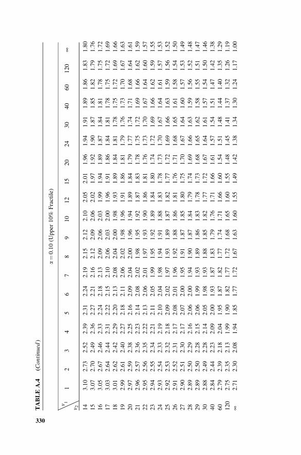
TABLEA.4
(Continued
)
a¼0.10(U
pper
10%
Fractile)
v 11
23
45
67
89
10
12
15
20
24
30
40
60
120
¥v 2 14
3.10
2.73
2.52
2.39
2.31
2.24
2.19
2.15
2.12
2.10
2.05
2.01
1.96
1.94
1.91
1.89
1.86
1.83
1.80
15
3.07
2.70
2.49
2.36
2.27
2.21
2.16
2.12
2.09
2.06
2.02
1.97
1.92
1.90
1.87
1.85
1.82
1.79
1.76
16
3.05
2.67
2.46
2.33
2.24
2.18
2.13
2.09
2.06
2.03
1.99
1.94
1.89
1.87
1.84
1.81
1.78
1.75
1.72
17
3.03
2.64
2.44
2.31
2.22
2.15
2.10
2.06
2.03
2.00
1.96
1.91
1.86
1.84
1.81
1.78
1.75
1.72
1.69
18
3.01
2.62
2.42
2.29
2.20
2.13
2.08
2.04
2.00
1.98
1.93
1.89
1.84
1.81
1.78
1.75
1.72
1.69
1.66
19
2.99
2.61
2.40
2.27
2.18
2.11
2.06
2.02
1.98
1.96
1.91
1.86
1.81
1.79
1.76
1.73
1.70
1.67
1.63
20
2.97
2.59
2.38
2.25
2.16
2.09
2.04
2.00
1.96
1.94
1.89
1.84
1.79
1.77
1.74
1.71
1.68
1.64
1.61
21
2.96
2.57
2.36
2.23
2.14
2.08
2.02
1.98
1.95
1.92
1.87
1.83
1.78
1.75
1.72
1.69
1.66
1.62
1.59
22
2.95
2.56
2.35
2.22
2.13
2.06
2.01
1.97
1.93
1.90
1.86
1.81
1.76
1.73
1.70
1.67
1.64
1.60
1.57
23
2.94
2.55
2.34
2.21
2.11
2.05
1.99
1.95
1.92
1.89
1.84
1.80
1.74
1.72
1.69
1.66
1.62
1.59
1.55
24
2.93
2.54
2.33
2.19
2.10
2.04
1.98
1.94
1.91
1.88
1.83
1.78
1.73
1.70
1.67
1.64
1.61
1.57
1.53
25
2.92
2.53
2.32
2.18
2.09
2.02
1.97
1.93
1.89
1.87
1.82
1.77
1.72
1.69
1.66
1.63
1.59
1.56
1.52
26
2.91
2.52
2.31
2.17
2.08
2.01
1.96
1.92
1.88
1.86
1.81
1.76
1.71
1.68
1.65
1.61
1.58
1.54
1.50
27
2.90
2.51
2.30
2.17
2.07
2.00
1.95
1.91
1.87
1.85
1.80
1.75
1.70
1.67
1.64
1.60
1.57
1.53
1.49
28
2.89
2.50
2.29
2.16
2.06
2.00
1.94
1.90
1.87
1.84
1.79
1.74
1.69
1.66
1.63
1.59
1.56
1.52
1.48
29
2.89
2.50
2.28
2.15
2.06
1.99
1.93
1.89
1.86
1.83
1.78
1.73
1.68
1.65
1.62
1.58
1.55
1.51
1.47
30
2.88
2.49
2.28
2.14
2.05
1.98
1.93
1.88
1.85
1.82
1.77
1.72
1.67
1.64
1.61
1.57
1.54
1.50
1.46
40
2.84
2.44
2.23
2.09
2.00
1.93
1.87
1.83
1.79
1.76
1.71
1.66
1.61
1.57
1.54
1.51
1.47
1.42
1.38
60
2.79
2.39
2.18
2.04
1.95
1.87
1.82
1.77
1.74
1.71
1.66
1.60
1.54
1.51
1.48
1.44
1.40
1.35
1.29
120
2.75
2.35
2.13
1.99
1.90
1.82
1.77
1.72
1.68
1.65
1.60
1.55
1.48
1.45
1.41
1.37
1.32
1.26
1.19
¥2.71
2.30
2.08
1.94
1.85
1.77
1.72
1.67
1.63
1.60
1.55
1.49
1.42
1.38
1.34
1.30
1.24
1.17
1.00
330
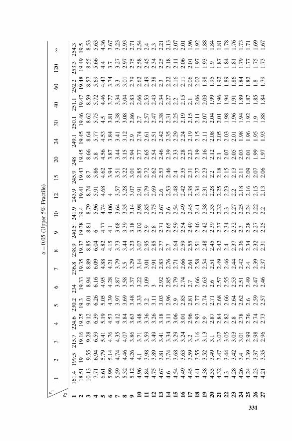
a¼0.05(U
pper
5%
Fractile)
v 11
23
45
67
89
10
12
15
20
24
30
40
60
120
¥v 2 1
161.4
199.5
215.7
224.6
230.2
234
236.8
238.9
240.5
241.9
243.9
245.9
248
249.1
250.1
251.1
252.2
253.3
254.3
218.51
19
19.16
19.25
19.3
19.33
19.35
19.37
19.38
19.4
19.41
19.43
19.45
19.45
19.46
19.47
19.48
19.49
19.5
310.13
9.55
9.28
9.12
9.01
8.94
8.89
8.85
8.81
8.79
8.74
8.7
8.66
8.64
8.62
8.59
8.57
8.55
8.53
47.71
6.94
6.59
6.39
6.26
6.16
6.09
6.04
65.96
5.91
5.86
5.8
5.77
5.75
5.72
5.69
5.66
5.63
56.61
5.79
5.41
5.19
5.05
4.95
4.88
4.82
4.77
4.74
4.68
4.62
4.56
4.53
4.5
4.46
4.43
4.4
4.36
65.99
5.14
4.76
4.53
4.39
4.28
4.21
4.15
4.1
4.06
43.94
3.87
3.84
3.81
3.77
3.74
3.7
3.67
75.59
4.74
4.35
4.12
3.97
3.87
3.79
3.73
3.68
3.64
3.57
3.51
3.44
3.41
3.38
3.34
3.3
3.27
3.23
85.32
4.46
4.07
3.84
3.69
3.58
3.5
3.44
3.39
3.35
3.28
3.22
3.15
3.12
3.08
3.04
3.01
2.97
2.93
95.12
4.26
3.86
3.63
3.48
3.37
3.29
3.23
3.18
3.14
3.07
3.01
2.94
2.9
2.86
2.83
2.79
2.75
2.71
10
4.96
4.1
3.71
3.48
3.33
3.22
3.14
3.07
3.02
2.98
2.91
2.85
2.77
2.74
2.7
2.66
2.62
2.58
2.54
11
4.84
3.98
3.59
3.36
3.2
3.09
3.01
2.95
2.9
2.85
2.79
2.72
2.65
2.61
2.57
2.53
2.49
2.45
2.4
12
4.75
3.89
3.49
3.26
3.11
32.91
2.85
2.8
2.75
2.69
2.62
2.54
2.51
2.47
2.43
2.38
2.34
2.3
13
4.67
3.81
3.41
3.18
3.03
2.92
2.83
2.77
2.71
2.67
2.6
2.53
2.46
2.42
2.38
2.34
2.3
2.25
2.21
14
4.6
3.74
3.34
3.11
2.96
2.85
2.76
2.7
2.65
2.6
2.53
2.46
2.39
2.35
2.31
2.27
2.22
2.18
2.13
15
4.54
3.68
3.29
3.06
2.9
2.79
2.71
2.64
2.59
2.54
2.48
2.4
2.33
2.29
2.25
2.2
2.16
2.11
2.07
16
4.49
3.63
3.24
3.01
2.85
2.74
2.66
2.59
2.54
2.49
2.42
2.35
2.28
2.24
2.19
2.15
2.11
2.06
2.01
17
4.45
3.59
3.2
2.96
2.81
2.7
2.61
2.55
2.49
2.45
2.38
2.31
2.23
2.19
2.15
2.1
2.06
2.01
1.96
18
4.41
3.55
3.16
2.93
2.77
2.66
2.58
2.51
2.46
2.41
2.34
2.27
2.19
2.15
2.11
2.06
2.02
1.97
1.92
19
4.38
3.52
3.13
2.9
2.74
2.63
2.54
2.48
2.42
2.38
2.31
2.23
2.16
2.11
2.07
2.03
1.98
1.93
1.88
20
4.35
3.49
3.1
2.87
2.71
2.6
2.51
2.45
2.39
2.35
2.28
2.2
2.12
2.08
2.04
1.99
1.95
1.9
1.84
21
4.32
3.47
3.07
2.84
2.68
2.57
2.49
2.42
2.37
2.32
2.25
2.18
2.1
2.05
2.01
1.96
1.92
1.87
1.81
22
4.3
3.44
3.05
2.82
2.66
2.55
2.46
2.4
2.34
2.3
2.23
2.15
2.07
2.03
1.98
1.94
1.89
1.84
1.78
23
4.28
3.42
3.03
2.8
2.64
2.53
2.44
2.37
2.32
2.27
2.2
2.13
2.05
2.01
1.96
1.91
1.86
1.81
1.76
24
4.26
3.4
3.01
2.78
2.62
2.51
2.42
2.36
2.3
2.25
2.18
2.11
2.03
1.98
1.94
1.89
1.84
1.79
1.73
25
4.24
3.39
2.99
2.76
2.6
2.49
2.4
2.34
2.28
2.24
2.16
2.09
2.01
1.96
1.92
1.87
1.82
1.77
1.71
26
4.23
3.37
2.98
2.74
2.59
2.47
2.39
2.32
2.27
2.22
2.15
2.07
1.99
1.95
1.9
1.85
1.8
1.75
1.69
27
4.21
3.35
2.96
2.73
2.57
2.46
2.37
2.31
2.25
2.2
2.13
2.06
1.97
1.93
1.88
1.84
1.79
1.73
1.67
331
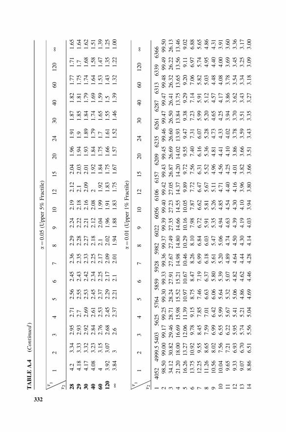
TABLEA.4
(Continued
)
a¼0.05(U
pper
5%
Fractile)
v 11
23
45
67
89
10
12
15
20
24
30
40
60
120
¥v 2 28
4.2
3.34
2.95
2.71
2.56
2.45
2.36
2.29
2.24
2.19
2.12
2.04
1.96
1.91
1.87
1.82
1.77
1.71
1.65
29
4.18
3.33
2.93
2.7
2.55
2.43
2.35
2.28
2.22
2.18
2.1
2.03
1.94
1.9
1.85
1.81
1.75
1.7
1.64
30
4.17
3.32
2.92
2.69
2.53
2.42
2.33
2.27
2.21
2.16
2.09
2.01
1.93
1.89
1.84
1.79
1.74
1.68
1.62
40
4.08
3.23
2.84
2.61
2.45
2.34
2.25
2.18
2.12
2.08
21.92
1.84
1.79
1.74
1.69
1.64
1.58
1.51
60
43.15
2.76
2.53
2.37
2.25
2.17
2.1
2.04
1.99
1.92
1.84
1.75
1.7
1.65
1.59
1.53
1.47
1.39
120
3.92
3.07
2.68
2.45
2.29
2.17
2.09
2.02
1.96
1.91
1.83
1.75
1.66
1.61
1.55
1.5
1.43
1.35
1.25
¥3.84
32.6
2.37
2.21
2.1
2.01
1.94
1.88
1.83
1.75
1.67
1.57
1.52
1.46
1.39
1.32
1.22
1.00
a¼0.01(U
pper
1%
Fractile)
v 11
23
45
67
89
10
12
15
20
24
30
40
60
120
¥v 2 1
4052
4999.5
5403
5625
5764
5859
5928
5982
6022
6056
6106
6157
6209
6235
6261
6287
6313
6339
6366
298.50
99.00
99.17
99.25
99.30
99.33
99.36
99.37
99.39
99.40
99.42
99.43
99.45
99.46
99.47
99.47
99.48
99.49
99.50
334.12
30.82
29.46
28.71
28.24
27.91
27.67
27.49
27.35
27.23
27.05
26.87
26.69
26.60
26.50
26.41
26.32
26.22
26.13
421.20
18.00
16.69
15.98
15.52
15.21
14.98
14.80
14.66
14.55
14.37
14.20
14.02
13.93
13.84
13.75
13.65
13.56
13.46
516.26
13.27
12.06
11.39
10.97
10.67
10.46
10.29
10.16
10.05
9.89
9.72
9.55
9.47
9.38
9.29
9.20
9.11
9.02
613.75
10.92
9.78
9.15
8.75
8.47
8.26
8.10
7.98
7.87
7.72
7.56
7.40
7.31
7.23
7.14
7.06
6.97
6.88
712.25
9.55
8.45
7.85
7.46
7.19
6.99
6.84
6.72
6.62
6.47
6.31
6.16
6.07
5.99
5.91
5.82
5.74
5.65
811.26
8.65
7.59
7.01
6.63
6.37
6.18
6.03
5.91
5.81
5.67
5.52
5.36
5.28
5.20
5.12
5.03
4.95
4.86
910.56
8.02
6.99
6.42
6.06
5.80
5.61
5.47
5.35
5.26
5.11
4.96
4.81
4.73
4.65
4.57
4.48
4.40
4.31
10
10.04
7.56
6.55
5.99
5.64
5.39
5.20
5.06
4.94
4.85
4.71
4.56
4.41
4.33
4.25
4.17
4.08
4.00
3.91
11
9.65
7.21
6.22
5.67
5.32
5.07
4.89
4.74
4.63
4.54
4.40
4.25
4.10
4.02
3.94
3.86
3.78
3.69
3.60
12
9.33
6.93
5.95
5.41
5.06
4.82
4.64
4.50
4.39
4.30
4.16
4.01
3.86
3.78
3.70
3.62
3.54
3.45
3.36
13
9.07
6.70
5.74
5.21
4.86
4.62
4.44
4.30
4.19
4.10
3.96
3.82
3.66
3.59
3.51
3.43
3.34
3.25
3.17
14
8.86
6.51
5.56
5.04
4.69
4.46
4.28
4.14
4.03
3.94
3.80
3.66
3.51
3.43
3.35
3.27
3.18
3.09
3.00
332
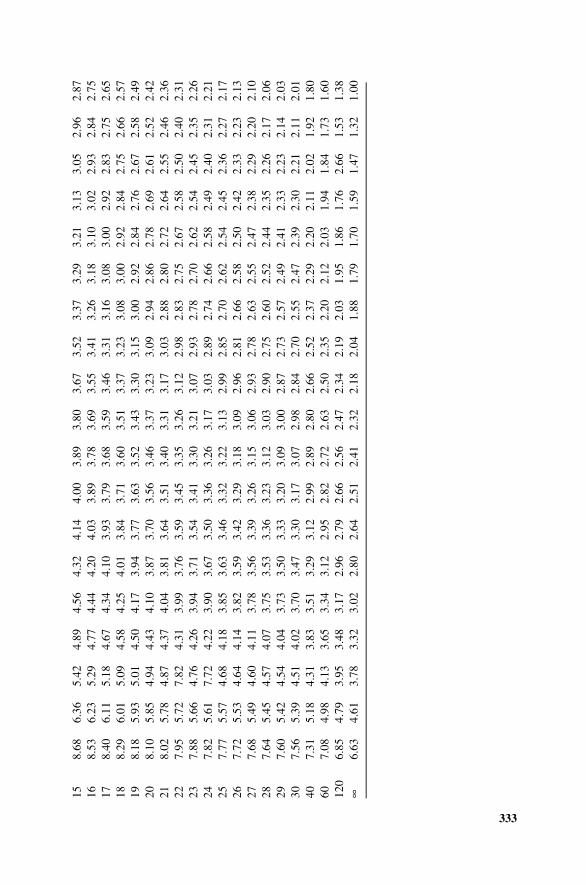
15
8.68
6.36
5.42
4.89
4.56
4.32
4.14
4.00
3.89
3.80
3.67
3.52
3.37
3.29
3.21
3.13
3.05
2.96
2.87
16
8.53
6.23
5.29
4.77
4.44
4.20
4.03
3.89
3.78
3.69
3.55
3.41
3.26
3.18
3.10
3.02
2.93
2.84
2.75
17
8.40
6.11
5.18
4.67
4.34
4.10
3.93
3.79
3.68
3.59
3.46
3.31
3.16
3.08
3.00
2.92
2.83
2.75
2.65
18
8.29
6.01
5.09
4.58
4.25
4.01
3.84
3.71
3.60
3.51
3.37
3.23
3.08
3.00
2.92
2.84
2.75
2.66
2.57
19
8.18
5.93
5.01
4.50
4.17
3.94
3.77
3.63
3.52
3.43
3.30
3.15
3.00
2.92
2.84
2.76
2.67
2.58
2.49
20
8.10
5.85
4.94
4.43
4.10
3.87
3.70
3.56
3.46
3.37
3.23
3.09
2.94
2.86
2.78
2.69
2.61
2.52
2.42
21
8.02
5.78
4.87
4.37
4.04
3.81
3.64
3.51
3.40
3.31
3.17
3.03
2.88
2.80
2.72
2.64
2.55
2.46
2.36
22
7.95
5.72
7.82
4.31
3.99
3.76
3.59
3.45
3.35
3.26
3.12
2.98
2.83
2.75
2.67
2.58
2.50
2.40
2.31
23
7.88
5.66
4.76
4.26
3.94
3.71
3.54
3.41
3.30
3.21
3.07
2.93
2.78
2.70
2.62
2.54
2.45
2.35
2.26
24
7.82
5.61
7.72
4.22
3.90
3.67
3.50
3.36
3.26
3.17
3.03
2.89
2.74
2.66
2.58
2.49
2.40
2.31
2.21
25
7.77
5.57
4.68
4.18
3.85
3.63
3.46
3.32
3.22
3.13
2.99
2.85
2.70
2.62
2.54
2.45
2.36
2.27
2.17
26
7.72
5.53
4.64
4.14
3.82
3.59
3.42
3.29
3.18
3.09
2.96
2.81
2.66
2.58
2.50
2.42
2.33
2.23
2.13
27
7.68
5.49
4.60
4.11
3.78
3.56
3.39
3.26
3.15
3.06
2.93
2.78
2.63
2.55
2.47
2.38
2.29
2.20
2.10
28
7.64
5.45
4.57
4.07
3.75
3.53
3.36
3.23
3.12
3.03
2.90
2.75
2.60
2.52
2.44
2.35
2.26
2.17
2.06
29
7.60
5.42
4.54
4.04
3.73
3.50
3.33
3.20
3.09
3.00
2.87
2.73
2.57
2.49
2.41
2.33
2.23
2.14
2.03
30
7.56
5.39
4.51
4.02
3.70
3.47
3.30
3.17
3.07
2.98
2.84
2.70
2.55
2.47
2.39
2.30
2.21
2.11
2.01
40
7.31
5.18
4.31
3.83
3.51
3.29
3.12
2.99
2.89
2.80
2.66
2.52
2.37
2.29
2.20
2.11
2.02
1.92
1.80
60
7.08
4.98
4.13
3.65
3.34
3.12
2.95
2.82
2.72
2.63
2.50
2.35
2.20
2.12
2.03
1.94
1.84
1.73
1.60
120
6.85
4.79
3.95
3.48
3.17
2.96
2.79
2.66
2.56
2.47
2.34
2.19
2.03
1.95
1.86
1.76
2.66
1.53
1.38
¥6.63
4.61
3.78
3.32
3.02
2.80
2.64
2.51
2.41
2.32
2.18
2.04
1.88
1.79
1.70
1.59
1.47
1.32
1.00
333
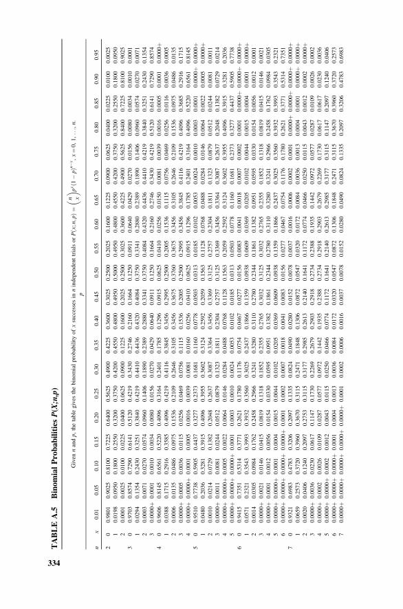
TABLEA.5
BinomialProbabilitiesP(X;n,p)
Given
nandp,thetable
gives
thebinomialprobabilityofxsuccessesin
nindependenttrialsorPx;n;p
ðÞ¼
n x�� p
x1�p
ðÞn�
x,x¼0,1,...,n.
p
nx
0.01
0.05
0.10
0.15
0.20
0.25
0.30
0.35
0.40
0.45
0.50
0.55
0.60
0.65
0.70
0.75
0.80
0.85
0.90
0.95
20
0.9801
0.9025
0.8100
0.7225
0.6400
0.5625
0.4900
0.4225
0.3600
0.3025
0.2500
0.2025
0.1600
0.1225
0.0900
0.0625
0.0400
0.0225
0.0100
0.0025
10.0198
0.0950
0.1800
0.2550
0.3200
0.3750
0.4200
0.4550
0.4800
0.4950
0.5000
0.4950
0.4800
0.4550
0.4200
0.3750
0.3200
0.2550
0.1800
0.0950
20.0001
0.0025
0.0100
0.0225
0.0400
0.0625
0.0900
0.1225
0.1600
0.2025
0.2500
0.3025
0.3600
0.4225
0.4900
0.5625
0.8400
0.7225
0.8100
0.9025
30
0.9703
0.8574
0.7290
0.6141
0.5120
0.4219
0.3430
0.2746
0.2160
0.1664
0.1250
0.0911
0.0640
0.0429
0.0270
0.0156
0.0080
0.0034
0.0010
0.0001
10.0294
0.1354
0.2430
0.3251
0.3840
0.4219
0.4410
0.4436
0.4320
0.4084
0.3750
0.3341
0.2880
0.2389
0.1890
0.1406
0.0960
0.0574
0.0270
0.0071
20.0003
0.0071
0.0270
0.0574
0.0960
0.1406
0.1890
0.2389
0.2880
0.3341
0.3750
0.4084
0.4320
0.4436
0.4410
0.4219
0.3840
0.3251
0.2430
0.1354
30.0000þ
0.0001
0.0010
0.0034
0.0080
0.0156
0.0270
0.0429
0.0640
0.0911
0.1250
0.1664
0.2160
0.2746
0.3430
0.4219
0.5120
0.6141
0.7290
0.8574
40
0.9606
0.8145
0.6561
0.5220
0.4096
0.3164
0.2401
0.1785
0.1296
0.0915
0.0625
0.0410
0.0256
0.0150
0.0081
0.0039
0.0016
0.0005
0.0001
0.0000þ
10.0388
0.1715
0.2916
0.3585
0.4096
0.4219
0.4116
0.3845
0.3456
0.2995
0.2500
0.2005
0.1536
0.1115
0.0756
0.0469
0.0256
0.0116
0.0036
0.0005
20.0006
0.0135
0.0486
0.0975
0.1536
0.2109
0.2646
0.3105
0.3456
0.3675
0.3760
0.3675
0.3456
0.3105
0.2646
0.2109
0.1536
0.0975
0.0486
0.0135
30.0000þ
0.0005
0.0036
0.0115
0.0256
0.0469
0.0756
0.1115
0.1536
0.2005
0.2500
0.2995
0.3456
0.3845
0.4116
0.4219
0.4096
0.3685
0.2916
0.1715
40.0000þ
0.0000þ
0.0001
0.0005
0.0016
0.0039
0.0081
0.0160
0.0256
0.0410
0.0625
0.0915
0.1296
0.1785
0.2401
0.3164
0.4096
0.5220
0.6561
0.8145
50
0.9510
0.7738
0.5905
0.4437
0.3277
0.2373
0.1681
0.1160
0.0778
0.0503
0.0313
0.0185
0.0102
0.0053
0.0024
0.0010
0.0003
0.0001
0.0000þ
0.0000þ
10.0480
0.2036
0.3281
0.3915
0.4096
0.3955
0.3602
0.3124
0.2592
0.2059
0.1563
0.1128
0.0768
0.0488
0.0284
0.0146
0.0064
0.0022
0.0005
0.0000þ
20.0010
0.0214
0.0729
0.1382
0.2048
0.2637
0.3087
0.3364
0.3456
0.3369
0.3125
0.2757
0.2304
0.1811
0.1323
0.0879
0.0512
0.0244
0.0081
0.0011
30.0000þ
0.0011
0.0081
0.0244
0.0512
0.0879
0.1323
0.1811
0.2304
0.2757
0.3125
0.3369
0.3456
0.3364
0.3087
0.2637
0.2048
0.1382
0.0729
0.0214
40.0000þ
0.0000þ
0.0005
0.0022
0.0064
0.0146
0.0284
0.0488
0.0768
0.1128
0.1563
0.2059
0.2592
0.3124
0.3602
0.3955
0.4096
0.3915
0.3281
0.2036
50.0000þ
0.0000þ
0.0000þ
0.0001
0.0003
0.0010
0.0024
0.0053
0.0102
0.0185
0.0313
0.0503
0.0778
0.1160
0.1681
0.2373
0.3277
0.4437
0.5905
0.7738
60
0.9415
0.7351
0.5314
0.3771
0.2621
0.1780
0.1176
0.0754
0.0467
0.0277
0.0156
0.0083
0.0041
0.0018
0.0007
0.0002
0.0001
0.0000þ
0.0000þ
0.0000þ
10.0571
0.2321
0.3543
0.3993
0.3932
0.3560
0.3025
0.2437
0.1866
0.1359
0.0938
0.0609
0.0369
0.0205
0.0102
0.0044
0.0015
0.0004
0.0001
0.0000þ
20.0014
0.0305
0.0984
0.1762
0.2458
0.2966
0.3241
0.3280
0.3110
0.2780
0.2344
0.1861
0.1382
0.0951
0.0595
0.0330
0.0154
0.0056
0.0012
0.0001
30.0000þ
0.0021
0.0146
0.0415
0.0819
0.1318
0.1852
0.2355
0.2765
0.3032
0.3125
0.3032
0.2765
0.2355
0.1852
0.1318
0.0819
0.0415
0.0146
0.0021
40.0000þ
0.0001
0.0012
0.0056
0.0154
0.0330
0.0595
0.0951
0.1382
0.1861
0.2344
0.2780
0.3110
0.3280
0.3241
0.2966
0.2458
0.1762
0.0984
0.0305
50.0000þ
0.0000þ
0.0001
0.0004
0.0015
0.0044
0.0102
0.0205
0.0369
0.0609
0.0938
0.1359
0.1866
0.2437
0.3025
0.3560
0.3932
0.3993
0.3543
0.2321
60.0000þ
0.0000þ
0.0000þ
0.0000þ
0.0001
0.0002
0.0007
0.0018
0.0041
0.0083
0.0156
0.0277
0.0467
0.0754
0.1176
0.1780
0.2621
0.3771
0.5314
0.7351
70
0.9321
0.6983
0.4783
0.3206
0.2097
0.1335
0.0824
0.0490
0.0280
0.0152
0.0078
0.0037
0.0016
0.0006
0.0002
0.0001
0.0000þ
0.0000þ
0.0000þ
0.0000þ
10.0659
0.2573
0.3720
0.3960
0.3670
0.3115
0.2471
0.1848
0.1306
0.0872
0.0547
0.0320
0.0172
0.0084
0.0036
0.0013
0.0004
0.0001
0.0000þ
0.0000þ
20.0020
0.0406
0.1240
0.2097
0.2753
0.3115
0.3177
0.2985
0.2613
0.2140
0.1641
0.1172
0.0774
0.0466
0.0250
0.0115
0.0043
0.0012
0.0002
0.0000þ
30.0000þ
0.0036
0.0230
0.0617
0.1147
0.1730
0.2269
0.2679
0.2903
0.2918
0.2734
0.2388
0.1935
0.1442
0.0972
0.0577
0.0287
0.0109
0.0026
0.0002
40.0000þ
0.0002
0.0026
0.0109
0.0287
0.0577
0.0972
0.1442
0.1935
0.2388
0.2734
0.2918
0.2903
0.2679
0.2269
0.1730
0.0617
0.0617
0.0230
0.0036
50.0000þ
0.0000þ
0.0002
0.0012
0.0043
0.0115
0.0250
0.0466
0.0774
0.1172
0.1641
0.2140
0.2613
0.2985
0.3177
0.3115
0.1147
0.2097
0.1240
0.0406
60.0000þ
0.0000þ
0.0000þ
0.0001
0.0004
0.0013
0.0036
0.0084
0.0172
0.0320
0.0547
0.0872
0.1306
0.1848
0.2471
0.3115
0.3670
0.3960
0.3720
0.2573
70.0000þ
0.0000þ
0.0000þ
0.0000þ
0.0000þ
0.0001
0.0002
0.0006
0.0016
0.0037
0.0078
0.0152
0.0280
0.0490
0.0824
0.1335
0.2097
0.3206
0.4783
0.6983
334
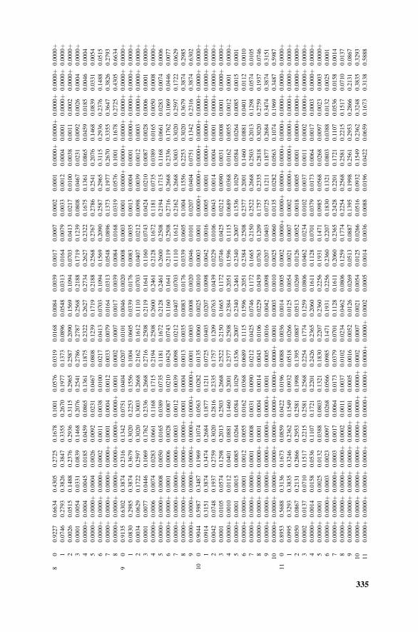
80
0.9227
0.6634
0.4305
0.2725
0.1678
0.1001
0.0576
0.0319
0.0168
0.0084
0.0039
0.0017
0.0007
0.0002
0.0001
0.0000þ
0.0000þ
0.0000þ
0.0000þ
0.0000þ
10.0746
0.2793
0.3826
0.3847
0.3355
0.2670
0.1977
0.1373
0.0896
0.0548
0.0313
0.0164
0.0079
0.0033
0.0012
0.0004
0.0001
0.0000þ
0.0000þ
0.0000þ
20.0026
0.0515
0.1488
0.2376
0.2936
0.3115
0.2965
0.2587
0.2090
0.1569
0.1094
0.0703
0.0413
0.0217
0.0100
0.0038
0.0011
0.0002
0.0000þ
0.0000þ
30.0001
0.0054
0.0331
0.0839
0.1468
0.2076
0.2541
0.2786
0.2787
0.2568
0.2188
0.1719
0.1239
0.0808
0.0467
0.0231
0.0092
0.0026
0.0004
0.0000þ
40.0000þ
0.0004
0.0045
0.0185
0.0459
0.0865
0.1361
0.1875
0.2322
0.2627
0.2734
0.2627
0.2322
0.1675
0.1361
0.0865
0.0459
0.0185
0.0046
0.0004
50.0000þ
0.0000þ
0.0004
0.0026
0.0092
0.0231
0.0467
0.0808
0.1239
0.1719
0.2188
0.2568
0.2767
0.2786
0.2541
0.2076
0.1468
0.0839
0.0331
0.0054
60.0000þ
0.0000þ
0.0000þ
0.0002
0.0011
0.0038
0.0100
0.0217
0.0413
0.0703
0.1094
0.1569
0.2090
0.2587
0.2965
0.3115
0.2936
0.2376
0.1488
0.0515
70.0000þ
0.0000þ
0.0000þ
0.0000þ
0.0001
0.0004
0.0012
0.0033
0.0079
0.0164
0.0313
0.0548
0.0896
0.1373
0.1977
0.2670
0.3355
0.3647
0.3826
0.2793
80.0000þ
0.0000þ
0.0000þ
0.0000þ
0.0000þ
0.0000þ
0.0001
0.0002
0.0007
0.0017
0.0039
0.0084
0.0168
0.0319
0.0576
0.1001
0.1678
0.2725
0.4305
0.6634
90
0.9135
0.6302
0.3874
0.2316
0.1342
0.0751
0.0404
0.0207
0.0101
0.0046
0.0020
0.0008
0.0003
0.0001
0.0000þ
0.0000þ
0.0000þ
0.0000þ
0.0000þ
0.0000þ
10.0830
0.2985
0.3874
0.3679
0.3020
0.2253
0.1556
0.1004
0.0605
0.0339
0.0176
0.0083
0.0035
0.0013
0.0004
0.0001
0.0000þ
0.0000þ
0.0000þ
0.0000þ
20.0034
0.0629
0.1722
0.2597
0.3020
0.3003
0.2668
0.2162
0.1612
0.1110
0.0703
0.0407
0.0212
0.0098
0.0039
0.0012
0.0003
0.0000þ
0.0000þ
0.0000þ
30.0001
0.0077
0.0446
0.1069
0.1762
0.2336
0.2668
0.2716
0.2508
0.2119
0.1641
0.1160
0.0743
0.0424
0.0210
0.0087
0.0028
0.0006
0.0001
0.0000þ
40.0000þ
0.0006
0.0074
0.0283
0.0661
0.1168
0.1715
0.2194
0.2508
0.2600
0.2461
0.2128
0.1672
0.1181
0.0735
0.0389
0.0165
0.0050
0.0008
0.0000þ
50.0000þ
0.0000þ
0.0008
0.0050
0.0165
0.0389
0.0735
0.1181
0.1672
0.2128
0.2461
0.2600
0.2508
0.2194
0.1715
0.1168
0.0661
0.0283
0.0074
0.0006
60.0000þ
0.0000þ
0.0001
0.0006
0.0028
0.0087
0.0210
0.0424
0.0743
0.1160
0.1641
0.2119
0.2508
0.2716
0.2668
0.2336
0.1762
0.1069
0.0446
0.0077
70.0000þ
0.0000þ
0.0000þ
0.0000þ
0.0003
0.0012
0.0039
0.0098
0.0212
0.0407
0.0703
0.1110
0.1612
0.2162
0.2668
0.3003
0.3020
0.2597
0.1722
0.0629
80.0000þ
0.0000þ
0.0000þ
0.0000þ
0.0000þ
0.0001
0.0004
0.0013
0.0035
0.0083
0.0176
0.0339
0.0605
0.1004
0.1556
0.2253
0.3020
0.3679
0.3874
0.2985
90.0000þ
0.0000þ
0.0000þ
0.0000þ
0.0000þ
0.0000þ
0.0000þ
0.0001
0.0003
0.0008
0.0020
0.0046
0.0101
0.0207
0.0404
0.0751
0.1342
0.2316
0.3874
0.6302
10
00.9044
0.5987
0.3487
0.1969
0.1074
0.0563
0.0282
0.0135
0.0060
0.0025
0.0010
0.0003
0.0001
0.0000þ
0.0000þ
0.0000þ
0.0000þ
0.0000þ
0.0000þ
0.0000þ
10.0914
0.3151
0.3874
0.3474
0.2684
0.1877
0.1211
0.0725
0.0403
0.0207
0.0098
0.0042
0.0016
0.0005
0.0001
0.0000þ
0.0000þ
0.0000þ
0.0000þ
0.0000þ
20.0042
0.0748
0.1937
0.2759
0.3020
0.2816
0.2335
0.1757
0.1209
0.0763
0.0439
0.0229
0.0106
0.0043
0.0014
0.0004
0.0001
0.0000þ
0.0000þ
0.0000þ
30.0001
0.0105
0.0574
0.1298
0.2013
0.2503
0.2668
0.2522
0.2150
0.1665
0.1172
0.0746
0.0425
0.0212
0.0090
0.0031
0.0008
0.0001
0.0000þ
0.0000þ
40.0000þ
0.0010
0.0112
0.0401
0.0881
0.1460
0.2001
0.2377
0.2508
0.2384
0.2051
0.1596
0.1115
0.0689
0.0368
0.0162
0.0055
0.0012
0.0001
0.0000þ
50.0000þ
0.0001
0.0015
0.0085
0.0264
0.0584
0.1029
0.1536
0.2007
0.2340
0.2461
0.2340
0.2007
0.1536
0.1029
0.0584
0.0264
0.0085
0.0015
0.0001
60.0000þ
0.0000þ
0.0001
0.0012
0.0055
0.0162
0.0368
0.0689
0.1115
0.1596
0.2051
0.2384
0.2508
0.2377
0.2001
0.1460
0.0881
0.0401
0.0112
0.0010
70.0000þ
0.0000þ
0.0000þ
0.0001
0.0008
0.0031
0.0090
0.0212
0.0425
0.0746
0.1172
0.1665
0.2150
0.2522
0.2668
0.2503
0.2013
0.1298
0.0574
0.0105
80.0000þ
0.0000þ
0.0000þ
0.0000þ
0.0001
0.0004
0.0014
0.0043
0.0106
0.0229
0.0439
0.0763
0.1209
0.1757
0.2335
0.2818
0.3020
0.2759
0.1937
0.0746
90.0000þ
0.0000þ
0.0000þ
0.0000þ
0.0000þ
0.0000þ
0.0001
0.0005
0.0016
0.0042
0.0098
0.0207
0.0403
0.0725
0.1211
0.1877
0.2684
0.3474
0.3874
0.3151
10
0.0000þ
0.0000þ
0.0000þ
0.0000þ
0.0000þ
0.0000þ
0.0000þ
0.0000þ
0.0001
0.0003
0.0010
0.0025
0.0060
0.0135
0.0282
0.0563
0.1074
0.1969
0.3487
0.5987
11
00.8953
0.5688
0.3136
0.1673
0.0859
0.0422
0.0196
0.0088
0.0036
0.0014
0.0005
0.0002
0.0000þ
0.0000þ
0.0000þ
0.0000þ
0.0000þ
0.0000þ
0.0000þ
0.0000þ
10.0995
0.3293
0.3835
0.3246
0.2362
0.1549
0.0932
0.0518
0.0266
0.0125
0.0054
0.0021
0.0007
0.0002
0.0000þ
0.0000þ
0.0000þ
0.0000þ
0.0000þ
0.0000þ
20.0050
0.0867
0.2131
0.2866
0.2953
0.2581
0.1998
0.1395
0.0887
0.0513
0.0269
0.0126
0.0052
0.0018
0.0005
0.0001
0.0000þ
0.0000þ
0.0000þ
0.0000þ
30.0002
0.0137
0.0710
0.1517
0.2215
0.2581
0.2568
0.2254
0.1774
0.1259
0.0806
0.0462
0.0234
0.0102
0.0037
0.0011
0.0002
0.0000þ
0.0000þ
0.0000þ
40.0000þ
0.0014
0.0158
0.0536
0.1107
0.1721
0.2201
0.2426
0.2365
0.2060
0.1611
0.1128
0.0701
0.0379
0.0173
0.0064
0.0017
0.0003
0.0000þ
0.0000þ
50.0000þ
0.0001
0.0025
0.0132
0.0388
0.0803
0.1321
0.1830
0.2207
0.2360
0.2256
0.1931
0.1471
0.0985
0.0568
0.0268
0.0097
0.0023
0.0003
0.0000þ
60.0000þ
0.0000þ
0.0003
0.0023
0.0097
0.0268
0.0566
0.0985
0.1471
0.1931
0.2256
0.2360
0.2207
0.1830
0.1321
0.0803
0.0388
0.0132
0.0025
0.0001
70.0000þ
0.0000þ
0.0000þ
0.0003
0.0017
0.0064
0.0173
0.0379
0.0701
0.1128
0.1611
0.2060
0.2365
0.2428
0.2201
0.1721
0.1107
0.0536
0.0158
0.0014
80.0000þ
0.0000þ
0.0000þ
0.0000þ
0.0002
0.0011
0.0037
0.0102
0.0234
0.0462
0.0806
0.1259
0.1774
0.2254
0.2568
0.2581
0.2215
0.1517
0.0710
0.0137
90.0000þ
0.0000þ
0.0000þ
0.0000þ
0.0000þ
0.0001
0.0005
0.0016
0.0052
0.0126
0.0269
0.0513
0.0887
0.1395
0.1998
0.2561
0.2953
0.2866
0.2131
0.0867
10
0.0000þ
0.0000þ
0.0000þ
0.0000þ
0.0000þ
0.0000þ
0.0000þ
0.0002
0.0007
0.0021
0.0054
0.0125
0.0266
0.0516
0.0932
0.1549
0.2362
0.3248
0.3835
0.3293
11
0.0000þ
0.0000þ
0.0000þ
0.0000þ
0.0000þ
0.0000þ
0.0000þ
0.0000þ
0.0000þ
0.0002
0.0005
0.0014
0.0036
0.0088
0.0196
0.0422
0.0659
0.1673
0.3138
0.5888
335
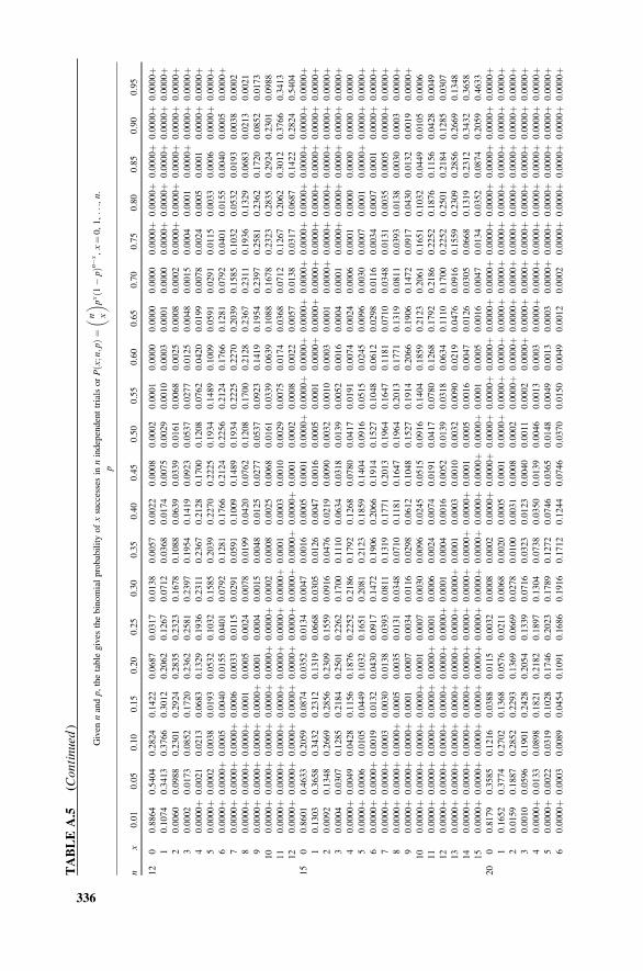
TABLEA.5
(Continued
)
Given
nandp,thetable
gives
thebinomialprobabilityofxsuccessesin
nindependenttrialsorPx;n;p
ðÞ¼
n x�� p
x1�p
ðÞn�
x,x¼0,1,...,n.
p
nx
0.01
0.05
0.10
0.15
0.20
0.25
0.30
0.35
0.40
0.45
0.50
0.55
0.60
0.65
0.70
0.75
0.80
0.85
0.90
0.95
12
00.8864
0.5404
0.2824
0.1422
0.0687
0.0317
0.0138
0.0057
0.0022
0.0008
0.0002
0.0001
0.0000
0.0000
0.0000
0.0000þ
0.0000þ
0.0000þ
0.0000þ
0.0000þ
10.1074
0.3413
0.3766
0.3012
0.2062
0.1267
0.0712
0.0368
0.0174
0.0075
0.0029
0.0010
0.0003
0.0001
0.0000
0.0000þ
0.0000þ
0.0000þ
0.0000þ
0.0000þ
20.0060
0.0988
0.2301
0.2924
0.2835
0.2323
0.1678
0.1088
0.0639
0.0339
0.0161
0.0068
0.0025
0.0008
0.0002
0.0000þ
0.0000þ
0.0000þ
0.0000þ
0.0000þ
30.0002
0.0173
0.0852
0.1720
0.2362
0.2581
0.2397
0.1954
0.1419
0.0923
0.0537
0.0277
0.0125
0.0048
0.0015
0.0004
0.0001
0.0000þ
0.0000þ
0.0000þ
40.0000þ
0.0021
0.0213
0.0683
0.1329
0.1936
0.2311
0.2367
0.2128
0.1700
0.1208
0.0762
0.0420
0.0199
0.0078
0.0024
0.0005
0.0001
0.0000þ
0.0000þ
50.0000þ
0.0002
0.0038
0.0193
0.0532
0.1032
0.1585
0.2039
0.2270
0.2225
0.1934
0.1489
0.1009
0.0591
0.0291
0.0115
0.0033
0.0006
0.0000þ
0.0000þ
60.0000þ
0.0000þ
0.0005
0.0040
0.0155
0.0401
0.0792
0.1281
0.1766
0.2124
0.2256
0.2124
0.1766
0.1281
0.0792
0.0401
0.0155
0.0040
0.0005
0.0000þ
70.0000þ
0.0000þ
0.0000þ
0.0006
0.0033
0.0115
0.0291
0.0591
0.1009
0.1489
0.1934
0.2225
0.2270
0.2039
0.1585
0.1032
0.0532
0.0193
0.0038
0.0002
80.0000þ
0.0000þ
0.0000þ
0.0001
0.0005
0.0024
0.0078
0.0199
0.0420
0.0762
0.1208
0.1700
0.2128
0.2367
0.2311
0.1936
0.1329
0.0683
0.0213
0.0021
90.0000þ
0.0000þ
0.0000þ
0.0000þ
0.0001
0.0004
0.0015
0.0048
0.0125
0.0277
0.0537
0.0923
0.1419
0.1954
0.2397
0.2581
0.2362
0.1720
0.0852
0.0173
10
0.0000þ
0.0000þ
0.0000þ
0.0000þ
0.0000þ
0.0000þ
0.0002
0.0008
0.0025
0.0068
0.0161
0.0339
0.0639
0.1088
0.1678
0.2323
0.2835
0.2924
0.2301
0.0988
11
0.0000þ
0.0000þ
0.0000þ
0.0000þ
0.0000þ
0.0000þ
0.0000þ
0.0001
0.0003
0.0010
0.0029
0.0075
0.0174
0.0368
0.0712
0.1267
0.2062
0.3012
0.3766
0.3413
12
0.0000þ
0.0000þ
0.0000þ
0.0000þ
0.0000þ
0.0000þ
0.0000þ
0.0000þ
0.0000þ
0.0001
0.0002
0.0008
0.0022
0.0057
0.0138
0.0317
0.0687
0.1422
0.2824
0.5404
15
00.8601
0.4633
0.2059
0.0874
0.0352
0.0134
0.0047
0.0016
0.0005
0.0001
0.0000þ
0.0000þ
0.0000þ
0.0000þ
0.0000þ
0.0000þ
0.0000þ
0.0000þ
0.0000þ
0.0000þ
10.1303
0.3658
0.3432
0.2312
0.1319
0.0668
0.0305
0.0126
0.0047
0.0016
0.0005
0.0001
0.0000þ
0.0000þ
0.0000þ
0.0000þ
0.0000þ
0.0000þ
0.0000þ
0.0000þ
20.0092
0.1348
0.2669
0.2856
0.2309
0.1559
0.0916
0.0476
0.0219
0.0090
0.0032
0.0010
0.0003
0.0001
0.0000þ
0.0000þ
0.0000þ
0.0000þ
0.0000þ
0.0000þ
30.0004
0.0307
0.1285
0.2184
0.2501
0.2262
0.1700
0.1110
0.0634
0.0318
0.0139
0.0052
0.0016
0.0004
0.0001
0.0000þ
0.0000þ
0.0000þ
0.0000þ
0.0000þ
40.0000þ
0.0049
0.0428
0.1156
0.1876
0.2252
0.2186
0.1792
0.1268
0.0780
0.0417
0.0191
0.0074
0.0024
0.0006
0.0001
0.0000
0.0000
0.0000
0.0000
50.0000þ
0.0006
0.0105
0.0449
0.1032
0.1651
0.2081
0.2123
0.1859
0.1404
0.0916
0.0515
0.0245
0.0096
0.0030
0.0007
0.0001
0.0000þ
0.0000þ
0.0000þ
60.0000þ
0.0000þ
0.0019
0.0132
0.0430
0.0917
0.1472
0.1906
0.2066
0.1914
0.1527
0.1048
0.0612
0.0298
0.0116
0.0034
0.0007
0.0001
0.0000þ
0.0000þ
70.0000þ
0.0000þ
0.0003
0.0030
0.0138
0.0393
0.0811
0.1319
0.1771
0.2013
0.1964
0.1647
0.1181
0.0710
0.0348
0.0131
0.0035
0.0005
0.0000þ
0.0000þ
80.0000þ
0.0000þ
0.0000þ
0.0005
0.0035
0.0131
0.0348
0.0710
0.1181
0.1647
0.1964
0.2013
0.1771
0.1319
0.0811
0.0393
0.0138
0.0030
0.0003
0.0000þ
90.0000þ
0.0000þ
0.0000þ
0.0001
0.0007
0.0034
0.0116
0.0298
0.0612
0.1048
0.1527
0.1914
0.2066
0.1906
0.1472
0.0917
0.0430
0.0132
0.0019
0.0000þ
10
0.0000þ
0.0000þ
0.0000þ
0.0000þ
0.0001
0.0007
0.0030
0.0096
0.0245
0.0515
0.0916
0.1404
0.1859
0.2123
0.2061
0.1651
0.1032
0.0449
0.0105
0.0006
11
0.0000þ
0.0000þ
0.0000þ
0.0000þ
0.0000þ
0.0001
0.0006
0.0024
0.0074
0.0191
0.0417
0.0780
0.1268
0.1792
0.2186
0.2252
0.1876
0.1156
0.0428
0.0049
12
0.0000þ
0.0000þ
0.0000þ
0.0000þ
0.0000þ
0.0000þ
0.0001
0.0004
0.0016
0.0052
0.0139
0.0318
0.0634
0.1110
0.1700
0.2252
0.2501
0.2184
0.1285
0.0307
13
0.0000þ
0.0000þ
0.0000þ
0.0000þ
0.0000þ
0.0000þ
0.0000þ
0.0001
0.0003
0.0010
0.0032
0.0090
0.0219
0.0476
0.0916
0.1559
0.2309
0.2856
0.2669
0.1348
14
0.0000þ
0.0000þ
0.0000þ
0.0000þ
0.0000þ
0.0000þ
0.0000þ
0.0000þ
0.0000þ
0.0001
0.0005
0.0016
0.0047
0.0126
0.0305
0.0668
0.1319
0.2312
0.3432
0.3658
15
0.0000þ
0.0000þ
0.0000þ
0.0000þ
0.0000þ
0.0000þ
0.0000þ
0.0000þ
0.0000þ
0.0000þ
0.0000þ
0.0001
0.0005
0.0016
0.0047
0.0134
0.0352
0.0874
0.2059
0.4633
20
00.8179
0.3585
0.1216
0.0388
0.0115
0.0032
0.0008
0.0002
0.0000þ
0.0000þ
0.0000þ
0.0000þ
0.0000þ
0.0000þ
0.0000þ
0.0000þ
0.0000þ
0.0000þ
0.0000þ
0.0000þ
10.1652
0.3774
0.2702
0.1368
0.0576
0.0211
0.0068
0.0020
0.0005
0.0001
0.0000þ
0.0000þ
0.0000þ
0.0000þ
0.0000þ
0.0000þ
0.0000þ
0.0000þ
0.0000þ
0.0000þ
20.0159
0.1887
0.2852
0.2293
0.1369
0.0669
0.0278
0.0100
0.0031
0.0008
0.0002
0.0000þ
0.0000þ
0.0000þ
0.0000þ
0.0000þ
0.0000þ
0.0000þ
0.0000þ
0.0000þ
30.0010
0.0596
0.1901
0.2428
0.2054
0.1339
0.0716
0.0323
0.0123
0.0040
0.0011
0.0002
0.0000þ
0.0000þ
0.0000þ
0.0000þ
0.0000þ
0.0000þ
0.0000þ
0.0000þ
40.0000þ
0.0133
0.0898
0.1821
0.2182
0.1897
0.1304
0.0738
0.0350
0.0139
0.0046
0.0013
0.0003
0.0000þ
0.0000þ
0.0000þ
0.0000þ
0.0000þ
0.0000þ
0.0000þ
50.0000þ
0.0022
0.0319
0.1028
0.1746
0.2023
0.1789
0.1272
0.0746
0.0365
0.0148
0.0049
0.0013
0.0003
0.0000þ
0.0000þ
0.0000þ
0.0000þ
0.0000þ
0.0000þ
60.0000þ
0.0003
0.0089
0.0454
0.1091
0.1686
0.1916
0.1712
0.1244
0.0746
0.0370
0.0150
0.0049
0.0012
0.0002
0.0000þ
0.0000þ
0.0000þ
0.0000þ
0.0000þ
336
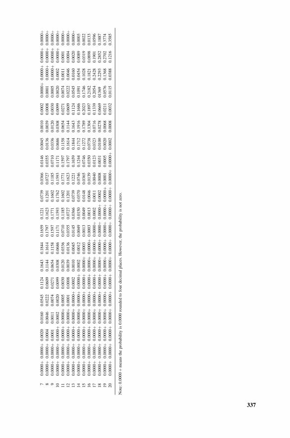
70.0000þ
0.0000þ
0.0020
0.0160
0.0545
0.1124
0.1643
0.1844
0.1659
0.1221
0.0739
0.0366
0.0146
0.0045
0.0010
0.0002
0.0000þ
0.0000þ
0.0000þ
0.0000þ
80.0000þ
0.0000þ
0.0004
0.0046
0.0222
0.0609
0.1144
0.1614
0.1797
0.1623
0.1201
0.0727
0.0355
0.0136
0.0039
0.0008
0.0001
0.0000þ
0.0000þ
0.0000þ
90.0000þ
0.0000þ
0.0001
0.0011
0.0074
0.0271
0.0654
0.1158
0.1597
0.1771
0.1602
0.1185
0.0710
0.0336
0.0120
0.0030
0.0005
0.0000þ
0.0000þ
0.0000þ
10
0.0000þ
0.0000þ
0.0000þ
0.0002
0.0020
0.0099
0.0308
0.0686
0.1171
0.1593
0.1762
0.1593
0.1171
0.0686
0.0308
0.0099
0.0020
0.0002
0.0000þ
0.0000þ
11
0.0000þ
0.0000þ
0.0000þ
0.0000þ
0.0005
0.0030
0.0120
0.0336
0.0710
0.1185
0.1602
0.1771
0.1597
0.1158
0.0654
0.0271
0.0074
0.0011
0.0001
0.0000þ
12
0.0000þ
0.0000þ
0.0000þ
0.0000þ
0.0001
0.0008
0.0039
0.0136
0.0355
0.0727
0.1201
0.1623
0.1797
0.1614
0.1144
0.0609
0.0222
0.0046
0.0004
0.0000þ
13
0.0000þ
0.0000þ
0.0000þ
0.0000þ
0.0000þ
0.0002
0.0010
0.0045
0.0145
0.0366
0.0739
0.1221
0.1659
0.1844
0.1643
0.1124
0.0545
0.0160
0.0020
0.0000þ
14
0.0000þ
0.0000þ
0.0000þ
0.0000þ
0.0000þ
0.0000þ
0.0002
0.0012
0.0049
0.0150
0.0370
0.0746
0.1244
0.1712
0.1916
0.1686
0.1091
0.0454
0.0089
0.0003
15
0.0000þ
0.0000þ
0.0000þ
0.0000þ
0.0000þ
0.0000þ
0.0000þ
0.0003
0.0013
0.0049
0.0148
0.0365
0.0746
0.1272
0.1789
0.2023
0.1746
0.1028
0.0319
0.0022
16
0.0000þ
0.0000þ
0.0000þ
0.0000þ
0.0000þ
0.0000þ
0.0000þ
0.0000þ
0.0003
0.0013
0.0046
0.0139
0.0350
0.0738
0.1304
0.1897
0.2182
0.1821
0.0898
0.0133
17
0.0000þ
0.0000þ
0.0000þ
0.0000þ
0.0000þ
0.0000þ
0.0000þ
0.0000þ
0.0000þ
0.0002
0.0011
0.0040
0.0123
0.0323
0.0716
0.1339
0.2054
0.2428
0.1901
0.0596
18
0.0000þ
0.0000þ
0.0000þ
0.0000þ
0.0000þ
0.0000þ
0.0000þ
0.0000þ
0.0000þ
0.0000þ
0.0002
0.0008
0.0031
0.0100
0.0278
0.0669
01369
0.2293
0.2852
0.1887
19
0.0000þ
0.0000þ
0.0000þ
0.0000þ
0.0000þ
0.0000þ
0.0000þ
0.0000þ
0.0000þ
0.0000þ
0.0000þ
0.0001
0.0005
0.0020
0.0068
0.0211
0.0576
0.1368
0.2702
0.3774
20
0.0000þ
0.0000þ
0.0000þ
0.0000þ
0.0000þ
0.0000þ
0.0000þ
0.0000þ
0.0000þ
0.0000þ
0.0000þ
0.0000þ
0.0000þ
0.0002
0.0008
0.0032
0.0115
0.0388
0.1216
0.3585
Note:0.0000þmeanstheprobabilityis0.0000rounded
tofourdecim
alplaces.However,theprobabilityisnotzero.
337
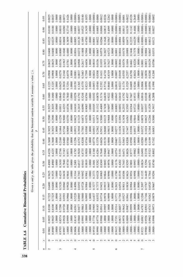
TABLEA.6
CumulativeBinomialProbabilities
Given
nandp,thetable
gives
theprobabilitythat
thebinomialrandom
variable
Xassumes
avalue�x.
p
nx
0.01
0.05
0.10
0.15
0.20
0.25
0.30
0.35
0.40
0.45
0.50
0.55
0.60
0.65
0.70
0.75
0.80
0.85
0.90
0.95
20
0.9801
0.9025
0.8100
0.7225
0.6400
0.5625
0.4900
0.4226
0.3600
0.3025
0.2500
0.2025
0.1600
0.1225
0.0900
0.0625
0.0400
0.0225
0.0100
0.0025
10.8989
0.9025
0.8100
0.7225
0.6400
0.5525
0.4900
0.4225
0.3600
0.3025
0.2500
0.2025
0.1600
0.1225
0.0900
0.0625
0.0400
0.0225
0.0100
0.0025
21.0000
1.0000
1.0000
1.0000
1.0000
1.0000
1.0000
1.0000
1.0000
1.0000
1.0000
1.0000
1.0000
1.0000
1.0000
1.0000
1.0000
1.0000
1.0000
1.0000
30
0.9703
0.8574
0.7290
0.6141
0.5120
0.4219
0.3430
0.2746
0.2160
0.1664
0.1250
0.0911
0.0640
0.0429
0.0270
0.0156
0.0080
0.0034
0.0010
0.0001
10.9997
0.9928
0.9720
0.9393
0.8960
0.8438
0.7840
0.7183
0.6480
0.5748
0.5000
0.4253
0.3520
0.2818
0.2160
0.1563
0.1040
0.0608
0.0280
0.0073
21.0000
0.9999
0.9990
0.9966
0.9920
0.9844
0.9730
0.9571
0.9360
0.9089
0.8750
0.8336
0.7840
0.7254
0.6570
0.5781
0.4880
0.3859
0.2710
0.1426
31.0000
1.0000
1.0000
1.0000
1.0000
1.0000
1.0000
1.0000
1.0000
1.0000
1.0000
1.0000
1.0000
1.0000
1.0000
1.0000
1.0000
1.0000
1.0000
1.0000
40
0.9606
0.8145
0.6561
0.5220
0.4096
0.3164
0.2401
0.1785
0.1296
0.0915
0.0625
0.0410
0.0258
0.0150
0.0081
0.0039
0.0016
0.0005
0.0001
0.0000þ
10.9994
0.9860
0.9477
0.8905
0.8192
0.7383
0.6517
0.5830
0.4752
0.3910
0.3125
0.2415
0.1792
0.1265
0.0837
0.0508
0.0272
0.0120
0.0037
0.0005
21.0000
0.9995
0.9863
0.9880
0.9728
0.9492
0.9163
0.8735
0.8208
0.7585
0.6875
0.6090
0.5248
0.4370
0.3483
0.2617
0.1808
0.1095
0.0523
0.0140
31.0000
1.0000
0.9999
0.9995
0.9984
0.9961
0.9819
0.9850
0.9744
0.9500
0.9376
0.9085
0.8704
0.8215
0.7599
0.6836
0.5904
0.4780
0.3439
0.1855
41.0000
1.0000
1.0000
1.0000
1.0000
1.0000
1.0000
1.0000
1.0000
1.0000
1.0000
1.0000
1.0000
1.0000
1.0000
1.0000
1.0000
1.0000
1.0000
1.0000
50
0.9510
0.7738
0.5905
0.4437
0.3277
0.2373
0.1681
0.1160
0.0778
0.0503
0.0313
0.0185
0.0102
0.0053
0.0024
0.0010
0.0003
0.0001
0.0000þ
0.0000þ
10.9990
0.9774
0.9185
0.8352
0.7373
0.6328
0.5282
0.4284
0.3370
0.2562
0.1875
0.1312
0.0870
0.0540
0.0308
0.0156
0.0067
0.0022
0.0005
0.0000
21.0000
0.9988
0.9914
0.9734
0.9421
0.8965
0.8369
0.7648
0.6826
0.5931
0.5000
0.4069
0.3174
0.2352
0.1631
0.1035
0.0579
0.0266
0.0086
0.0012
31.0000
1.0000
0.9995
0.9978
0.9933
0.9844
0.9692
0.9460
0.9130
0.8688
0.8125
0.7438
0.6630
0.5716
0.4718
0.3672
0.2627
0.1648
0.0815
0.0226
41.0000
1.0000
1.0000
0.9999
0.9997
0.9990
0.9976
0.9947
0.9898
0.9815
0.9688
0.9497
0.9222
0.8840
0.8319
0.7627
0.6723
0.5563
0.4095
0.2262
51.0000
1.0000
1.0000
1.0000
1.0000
1.0000
1.0000
1.0000
1.0000
1.0000
1.0000
1.0000
1.0000
1.0000
1.0000
1.0000
1.0000
1.0000
1.0000
1.0000
60
0.9415
0.7351
0.5314
0.3771
0.2621
0.1780
0.1176
0.0754
0.0467
0.0277
0.0156
0.0083
0.0043
0.0018
0.0007
0.0002
0.0001
0.0000þ
0.0000þ
0.0000þ
10.9985
0.9672
0.8857
0.7765
0.6554
0.5339
0.4202
0.3191
0.2333
0.1636
0.1094
0.0692
0.0410
0.0223
0.0109
0.0046
0.0016
0.0004
0.0001
0.0000þ
21.0000�
0.9978
0.9642
0.9527
0.9011
0.8306
0.7443
0.6471
0.5443
0.4415
0.3438
0.2553
0.1792
0.1174
0.0705
0.0376
0.0170
0.0059
0.0013
0.0001
31.0000�
0.9899
0.9987
0.9941
0.9830
0.9624
0.9295
0.8826
0.8208
0.7447
0.6563
0.5585
0.4557
0.3529
0.2557
0.1694
0.0989
0.0473
0.0159
0.0022
41.0000�
1.0000�
0.9999
0.9996
0.9984
0.9954
0.9891
0.9777
0.9590
0.9308
0.8906
0.8364
0.7667
0.6809
0.6798
0.4661
0.3446
0.2235
0.1143
0.0328
51.0000�
1.0000�
1.0000�
1.0000�
0.9989
0.9998
0.9993
0.9982
0.9959
0.8917
0.9844
0.9723
0.9533
0.9246
0.8824
0.8220
0.7379
0.6229
0.4686
0.2649
61.0000�
1.0000�
1.0000�
1.0000�
1.0000�
1.0000�
1.0000�
1.0000�
1.0000�
1.0000�
1.0000�
1.0000�
1.0000�
1.0000�
1.0000�
1.0000�
1.0000�
1.0000�
1.0000�
1.0000�
70
0.9321
0.6983
0.4783
0.3206
0.2097
0.1335
0.0824
0.0490
0.0280
0.0152
0.0078
0.0037
0.0016
0.0006
0.0002
0.0001
0.0000þ
0.0000þ
0.0000þ
0.0000þ
10.9980
0.9556
0.8503
0.7166
0.5767
0.4449
0.3294
0.2338
0.1586
0.1024
0.0625
0.0357
0.0188
0.0090
0.0038
0.0013
0.0004
0.0001
0.0000þ
0.0000þ
21.0000�
0.9962
0.9743
0.9262
0.8520
0.7564
0.6471
0.5323
0.4199
0.3164
0.2266
0.1529
0.0963
0.0556
0.0288
0.0129
0.0047
0.0012
0.0002
0.0000þ
31.0000�
0.9998
0.9973
0.9879
0.9667
0.9294
0.8740
0.8002
0.7102
0.6083
0.5000
0.3917
0.2898
0.1998
0.1260
0.0706
0.0333
0.0121
0.0027
0.0002
338
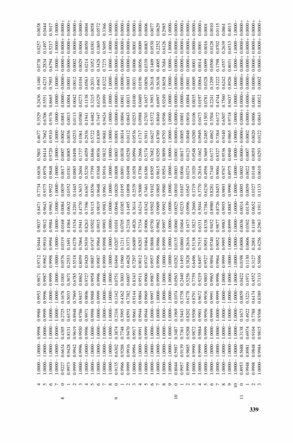
41.0000�
1.0000�
0.9998
0.9988
0.9953
0.9871
0.9712
0.9444
0.9037
0.8471
0.7734
0.6836
0.5801
0.4677
0.3529
0.2436
0.1480
0.0738
0.0257
0.0038
51.0000�
1.0000�
1.0000�
0.9999
0.9996
0.9987
0.9962
0.9910
0.9812
0.9643
0.9375
0.8976
0.8414
0.7662
0.6706
0.5551
0.4233
0.2834
0.1497
0.0444
61.0000�
1.0000�
1.0000�
1.0000�
1.0000�
0.9999
0.9998
0.9994
0.9984
0.9963
0.9922
0.9848
0.9720
0.9510
0.9176
0.8665
0.7903
0.6794
0.5217
0.3017
71.0000�
1.0000�
1.0000�
1.0000�
1.0000�
1.0000�
1.0000�
1.0000�
1.0000�
1.0000�
1.0000�
1.0000�
1.0000�
1.0000�
1.0000�
1.0000�
1.0000�
1.0000�
1.0000�
1.0000�
80
0.9227
0.6634
0.4305
0.2725
0.1678
0.1001
0.0576
0.0319
0.0168
0.0084
0.0039
0.0017
0.0007
0.0002
0.0001
0.0000þ
0.0000þ
0.0000þ
0.0000þ
0.0000þ
10.9973
0.9428
0.8131
0.6572
0.5033
0.3671
0.2553
0.1691
0.1064
0.0632
0.0352
0.0181
0.0085
0.0036
0.0013
0.0004
0.0001
0.0000þ
0.0000þ
0.0000þ
20.9999
0.9942
0.9619
0.8948
0.7969
0.6785
0.5518
0.4278
0.3154
0.2201
0.1445
0.0885
0.0498
0.0253
0.0113
0.0042
0.0012
0.0002
0.0000þ
0.0000þ
31.0000�
0.9996
0.9950
0.9786
0.9437
0.8862
0.8059
0.7064
0.5941
0.4770
0.3633
0.2604
0.1737
0.1061
0.0580
0.0273
0.0104
0.0029
0.0004
0.0000þ
41.0000�
1.0000�
0.9996
0.9971
0.9896
0.9727
0.9420
0.5939
0.8263
0.7396
0.6367
0.5230
0.4059
0.2936
0.1941
0.1138
0.0563
0.0214
0.0050
0.0004
51.0000�
1.0000�
1.0000�
0.9998
0.9988
0.9958
0.9887
0.9747
0.9502
0.9115
0.8556
0.7799
0.8846
0.5722
0.4482
0.3215
0.2031
0.1052
0.0381
0.0058
61.0000�
1.0000�
1.0000�
1.0000�
0.9999
0.9996
0.9987
0.9964
0.9915
0.9819
0.9648
0.9368
0.8936
0.8309
0.7447
0.6329
0.4967
0.3428
0.1869
0.0572
71.0000�
1.0000�
1.0000�
1.0000�
1.0000�
1.0000�
0.9999
0.9998
0.9993
0.9983
0.9961
0.9916
0.9832
0.9681
0.9424
0.8999
0.8322
0.7275
0.5695
0.3366
81.0000�
1.0000�
1.0000�
1.0000�
1.0000�
1.0000�
1.0000�
1.0000�
1.0000�
1.0000�
1.0000�
1.0000�
1.0000�
1.0000�
1.0000�
1.0000�
1.0000�
1.0000�
1.0000�
1.0000�
90
0.9135
0.6302
0.3874
0.2316
0.1342
0.0751
0.0404
0.0207
0.0101
0.0046
0.0020
0.0008
0.0003
0.0001
0.0000þ
0.0000þ
0.0000þ
0.0000þ
0.0000þ
0.0000þ
10.9966
0.9288
0.7748
0.5995
0.4362
0.3003
0.1960
0.1211
0.0705
0.0385
0.0195
0.0091
0.0038
0.0014
0.0004
0.0001
0.0000þ
0.0000þ
0.0000þ
0.0000þ
20.9999
0.9916
0.9470
0.8591
0.7382
0.6007
0.4628
0.3373
0.2318
0.1495
0.0898
0.0498
0.0250
0.0112
0.0043
0.0013
0.0003
0.0000þ
0.0000þ
0.0000þ
31.0000�
0.9994
0.9917
0.9661
0.9144
0.8343
0.7297
0.6089
0.4826
0.3614
0.2539
0.1658
0.0994
0.0536
0.0253
0.0100
0.0031
0.0006
0.0001
0.0000þ
41.0000�
1.0000�
0.9991
0.9944
0.9804
0.9511
0.9012
0.8283
0.7334
0.6214
0.5000
0.3786
0.2666
0.1717
0.0988
0.0489
0.0196
0.0056
0.0009
0.0000þ
51.0000�
1.0000�
0.9999
0.9944
0.9969
0.9900
0.9747
0.9464
0.9006
0.8342
0.7461
0.6386
0.5174
0.3911
0.2703
0.1657
0.0856
0.0339
0.0083
0.0006
61.0000�
1.0000�
1.0000�
1.0000�
0.9997
0.9987
0.9957
0.9888
0.9750
0.9502
0.9102
0.8505
0.7682
0.6627
0.5372
0.3993
0.2618
0.1409
0.0530
0.0077
71.0000�
1.0000�
1.0000�
1.0000�
1.0000�
0.9999
0.9996
0.9986
0.9962
0.9909
0.9805
0.9615
0.9295
0.8789
0.8040
0.6997
0.5638
0.4005
0.2252
0.0629
81.0000�
1.0000�
1.0000�
1.0000�
1.0000�
1.0000�
1.0000�
0.9999
0.9997
0.9992
0.9980
0.9954
0.9899
0.9793
0.9596
0.9249
0.8658
0.7684
0.6126
0.2985
91.0000�
1.0000�
1.0000�
1.0000�
1.0000�
1.0000�
1.0000�
1.0000�
1.0000�
1.0000�
1.0000�
1.0000�
1.0000�
1.0000�
1.0000�
1.0000�
1.0000�
1.0000�
1.0000�
1.0000�
10
00.8044
0.5987
0.3487
0.1969
0.1074
0.0563
0.0282
0.0135
0.0060
0.0025
0.0010
0.0003
0.0001
0.0000þ
0.0000þ
0.0000þ
0.0000þ
0.0000þ
0.0000þ
0.0000þ
10.9957
0.9139
0.7361
0.5443
0.3758
0.2440
0.1493
0.0860
0.0464
0.0233
0.0107
0.0046
0.0017
0.0005
0.0001
0.0000þ
0.0000þ
0.0000þ
0.0000þ
0.0000þ
20.9999
0.9885
0.9288
0.8202
0.6778
0.5256
0.3828
0.2616
0.1673
0.0996
0.0547
0.0274
0.0123
0.0048
0.0016
0.0004
0.0001
0.0000þ
0.0000þ
0.0000þ
31.0000�
0.9990
0.9872
0.9500
0.8791
0.7759
0.6496
0.5138
0.3823
0.2660
0.1719
0.1020
0.0548
0.0280
0.0106
0.0035
0.0009
0.0001
0.0000þ
0.0000þ
41.0000�
0.9999
0.9884
0.9901
0.9672
0.9219
0.8497
0.7515
0.6331
0.5044
0.3770
0.2616
0.1662
0.0949
0.0473
0.0197
0.0064
0.0014
0.0001
0.0000þ
51.0000�
1.0000�
0.9999
0.9956
0.9936
0.9803
0.9527
0.9051
0.8338
0.7384
0.6230
0.4956
0.3669
0.2485
0.1503
0.0781
0.0328
0.0099
0.0016
0.0001
61.0000�
1.0000�
1.0000�
0.9999
0.9991
0.9965
0.9894
0.9740
0.9452
0.8980
0.8281
0.7340
0.6177
0.4862
0.3504
0.2241
0.1209
0.0500
0.0128
0.0010
71.0000�
1.0000�
1.0000�
1.0000�
0.9999
0.9996
0.9964
0.9052
0.9877
0.8726
0.8453
0.9004
0.8327
0.7384
0.6172
0.4744
0.3222
0.1798
0.0702
0.0115
81.0000�
1.0000�
1.0000�
1.0000�
1.0000�
1.0000�
0.9999
0.9995
0.9983
0.9955
0.9893
0.9767
0.9536
0.9140
0.6507
0.7560
0.6242
0.4557
0.2639
0.0861
91.0000�
1.0000�
1.0000�
1.0000�
1.0000�
1.0000�
1.0000�
1.0000�
0.8999
0.8887
0.9990
0.8975
0.8940
0.9865
0.9718
0.9437
0.8926
0.8031
0.6513
0.4013
10
1.0000�
1.0000�
1.0000�
1.0000�
1.0000�
1.0000�
1.0000�
1.0000�
1.0000�
1.0000�
1.0000�
1.0000�
1.0000�
1.0000�
1.0000�
1.0000�
1.0000�
1.0000�
1.0000�
1.0000�
11
00.8953
0.5688
0.3138
0.1673
0.0859
0.0422
0.0198
0.0088
0.0036
0.0014
0.0005
0.0002
0.0000þ
0.0000þ
0.0000þ
0.0000þ
0.0000þ
0.0000þ
0.0000þ
0.0000þ
10.9948
0.8981
0.6974
0.4922
0.3221
0.1971
0.1130
0.0606
0.0302
0.0139
0.0059
0.0022
0.0007
0.0002
0.0000þ
0.0000þ
0.0000þ
0.0000þ
0.0000þ
0.0000þ
20.9998
0.9848
0.9104
0.7788
0.6174
0.4552
0.3127
0.2001
0.1189
0.0652
0.0327
0.0148
0.0059
0.0020
0.0006
0.0001
0.0000þ
0.0000þ
0.0000þ
0.0000þ
31.0000�
0.9984
0.9815
0.9306
0.8389
0.7133
0.5696
0.4256
0.2963
0.1911
0.1133
0.0610
0.0293
0.0122
0.0043
0.0012
0.0002
0.0000þ
0.0000þ
0.0000þ
339
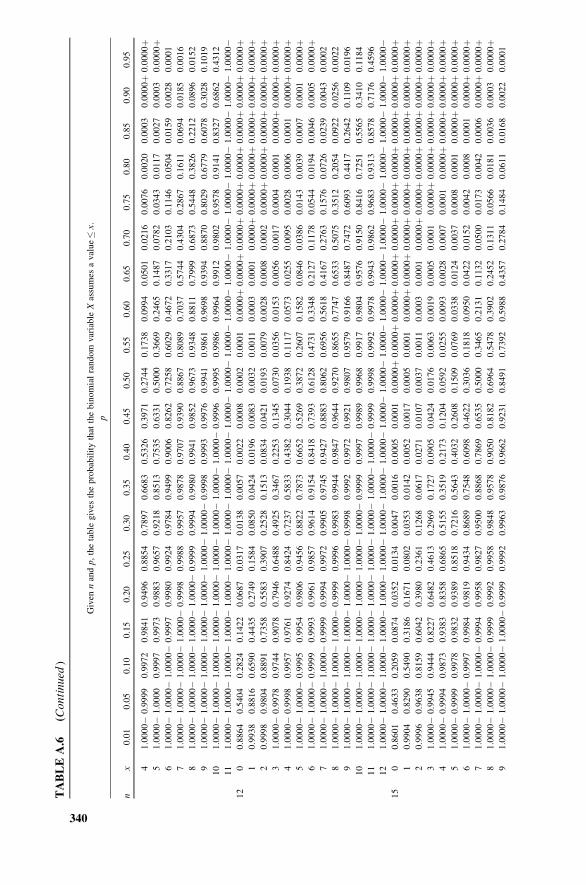
TABLEA.6
(Continued
)
Given
nandp,thetable
gives
theprobabilitythat
thebinomialrandom
variable
Xassumes
avalue�x.
p
nx
0.01
0.05
0.10
0.15
0.20
0.25
0.30
0.35
0.40
0.45
0.50
0.55
0.60
0.65
0.70
0.75
0.80
0.85
0.90
0.95
41.0000�
0.9999
0.9972
0.9841
0.9496
0.8854
0.7897
0.6683
0.5326
0.3971
0.2744
0.1738
0.0994
0.0501
0.0216
0.0076
0.0020
0.0003
0.0000þ
0.0000þ
51.0000�
1.0000
0.9997
0.9973
0.9883
0.9657
0.9218
0.8513
0.7535
0.6331
0.5000
0.3669
0.2465
0.1487
0.0782
0.0343
0.0117
0.0027
0.0003
0.0000þ
61.0000�
1.0000�
1.0000�
0.9997
0.9980
0.9924
0.9784
0.9499
0.9006
0.8262
0.7258
0.6029
0.4672
0.3317
0.2103
0.1146
0.0504
0.0159
0.0028
0.0001
71.0000�
1.0000�
1.0000�
1.0000�
0.9998
0.9988
0.9957
0.9878
0.9707
0.9390
0.8867
0.8089
0.7037
0.5744
0.4304
0.2867
0.1611
0.0694
0.0185
0.0016
81.0000�
1.0000�
1.0000�
1.0000�
1.0000�
0.9999
0.9994
0.9980
0.9941
0.9852
0.9673
0.9348
0.8811
0.7999
0.6873
0.5448
0.3826
0.2212
0.0896
0.0152
91.0000�
1.0000�
1.0000�
1.0000�
1.0000�
1.0000�
1.0000�
0.9998
0.9993
0.9976
0.9941
0.9861
0.9698
0.9394
0.8870
0.8029
0.6779
0.6078
0.3028
0.1019
10
1.0000�
1.0000�
1.0000�
1.0000�
1.0000�
1.0000�
1.0000�
1.0000�
1.0000�
0.9996
0.9995
0.9986
0.9964
0.9912
0.9802
0.9578
0.9141
0.8327
0.6862
0.4312
11
1.0000�
1.0000�
1.0000�
1.0000�
1.0000�
1.0000�
1.0000�
1.0000�
1.0000�
1.0000�
1.0000�
1.0000�
1.0000�
1.0000�
1.0000�
1.0000�
1.0000�
1.0000�
1.0000�
1.0000�
12
00.8864
0.5404
0.2824
0.1422
0.0687
0.0317
0.0138
0.0057
0.0022
0.0008
0.0002
0.0001
0.0000þ
0.0000þ
0.0000þ
0.0000þ
0.0000þ
0.0000þ
0.0000þ
0.0000þ
10.9938
0.8816
0.6590
0.4435
0.2749
0.1584
0.0850
0.0424
0.0196
0.0083
0.0032
0.0011
0.0003
0.0001
0.0000þ
0.0000þ
0.0000þ
0.0000þ
0.0000þ
0.0000þ
20.9998
0.9804
0.8891
0.7358
0.5583
0.3907
0.2528
0.1513
0.0834
0.0421
0.0193
0.0079
0.0028
0.0008
0.0002
0.0000þ
0.0000þ
0.0000þ
0.0000þ
0.0000þ
31.0000�
0.9978
0.9744
0.9078
0.7946
0.6488
0.4925
0.3467
0.2253
0.1345
0.0730
0.0356
0.0153
0.0056
0.0017
0.0004
0.0001
0.0000þ
0.0000þ
0.0000þ
41.0000�
0.9998
0.9957
0.9761
0.9274
0.8424
0.7237
0.5833
0.4382
0.3044
0.1938
0.1117
0.0573
0.0255
0.0095
0.0028
0.0006
0.0001
0.0000þ
0.0000þ
51.0000�
1.0000�
0.9995
0.9954
0.9806
0.9456
0.8822
0.7873
0.6652
0.5269
0.3872
0.2607
0.1582
0.0846
0.0386
0.0143
0.0039
0.0007
0.0001
0.0000þ
61.0000�
1.0000�
0.9999
0.9993
0.9961
0.9857
0.9614
0.9154
0.8418
0.7393
0.6128
0.4731
0.3348
0.2127
0.1178
0.0544
0.0194
0.0046
0.0005
0.0000þ
71.0000�
1.0000�
1.0000�
0.9999
0.9994
0.9972
0.9905
0.9745
0.9427
0.8883
0.8062
0.6956
0.5618
0.4167
0.2763
0.1576
0.0726
0.0239
0.0043
0.0002
81.0000�
1.0000�
1.0000�
1.0000�
0.9999
0.9996
0.9983
0.9944
0.9847
0.9644
0.9270
0.8655
0.7747
0.6533
0.5075
0.3512
0.2054
0.0922
0.0256
0.0022
91.0000�
1.0000�
1.0000�
1.0000�
1.0000�
1.0000�
0.9998
0.9992
0.9972
0.9921
0.9807
0.9579
0.9166
0.8487
0.7472
0.6093
0.4417
0.2642
0.1109
0.0196
10
1.0000�
1.0000�
1.0000�
1.0000�
1.0000�
1.0000�
1.0000�
0.9999
0.9997
0.9989
0.9968
0.9917
0.9804
0.9576
0.9150
0.8416
0.7251
0.5565
0.3410
0.1184
11
1.0000�
1.0000�
1.0000�
1.0000�
1.0000�
1.0000�
1.0000�
1.0000�
1.0000�
0.9999
0.9998
0.9992
0.9978
0.9943
0.9862
0.9683
0.9313
0.8578
0.7176
0.4596
12
1.0000�
1.0000�
1.0000�
1.0000�
1.0000�
1.0000�
1.0000�
1.0000�
1.0000�
1.0000�
1.0000�
1.0000�
1.0000�
1.0000�
1.0000�
1.0000�
1.0000�
1.0000�
1.0000�
1.0000�
15
00.8601
0.4633
0.2059
0.0874
0.0352
0.0134
0.0047
0.0016
0.0005
0.0001
0.0000þ
0.0000þ
0.0000þ
0.0000þ
0.0000þ
0.0000þ
0.0000þ
0.0000þ
0.0000þ
0.0000þ
10.9904
0.8290
0.5490
0.3186
0.1671
0.0802
0.0353
0.0142
0.0052
0.0017
0.0005
0.0001
0.0000þ
0.0000þ
0.0000þ
0.0000þ
0.0000þ
0.0000þ
0.0000þ
0.0000þ
20.9996
0.9638
0.8159
0.6042
0.3980
0.2361
0.1268
0.0617
0.0271
0.0107
0.0037
0.0011
0.0003
0.0001
0.0000þ
0.0000þ
0.0000þ
0.0000þ
0.0000þ
0.0000þ
31.0000�
0.9945
0.9444
0.8227
0.6482
0.4613
0.2969
0.1727
0.0905
0.0424
0.0176
0.0063
0.0019
0.0005
0.0001
0.0000þ
0.0000þ
0.0000þ
0.0000þ
0.0000þ
41.0000�
0.9994
0.9873
0.9383
0.8358
0.6865
0.5155
0.3519
0.2173
0.1204
0.0592
0.0255
0.0093
0.0028
0.0007
0.0001
0.0000þ
0.0000þ
0.0000þ
0.0000þ
51.0000�
0.9999
0.9978
0.9832
0.9389
0.8518
0.7216
0.5643
0.4032
0.2608
0.1509
0.0769
0.0338
0.0124
0.0037
0.0008
0.0001
0.0000þ
0.0000þ
0.0000þ
61.0000�
1.0000�
0.9997
0.9984
0.9819
0.9434
0.8689
0.7548
0.6098
0.4622
0.3036
0.1818
0.0950
0.0422
0.0152
0.0042
0.0008
0.0001
0.0000þ
0.0000þ
71.0000�
1.0000�
1.0000�
0.9994
0.9958
0.9827
0.9500
0.8868
0.7869
0.6535
0.5000
0.3465
0.2131
0.1132
0.0500
0.0173
0.0042
0.0006
0.0000þ
0.0000þ
81.0000�
1.0000�
1.0000�
0.9999
0.9992
0.9958
0.9848
0.9578
0.9050
0.8182
0.6964
0.5478
0.3902
0.2452
0.1311
0.0566
0.0181
0.0036
0.0003
0.0000þ
91.0000�
1.0000�
1.0000�
1.0000�
0.9999
0.9992
0.9963
0.9876
0.9662
0.9231
0.8491
0.7392
0.5988
0.4357
0.2784
0.1484
0.0611
0.0168
0.0022
0.0001
340
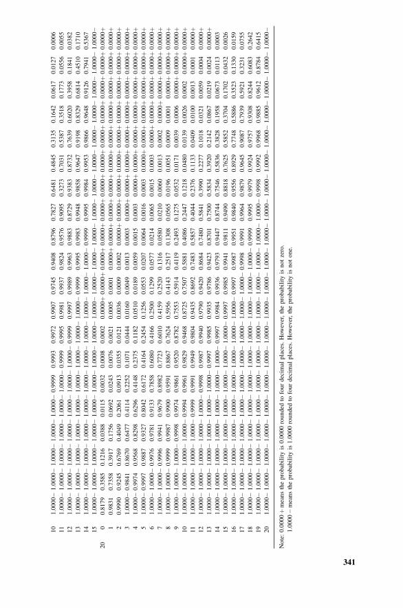
10
1.0000�
1.0000�
1.0000�
1.0000�
1.0000�
0.9999
0.9993
0.9972
0.9907
0.9745
0.9408
0.8796
0.7827
0.6481
0.4845
0.3135
0.1642
0.0617
0.0127
0.0006
11
1.0000�
1.0000�
1.0000�
1.0000�
1.0000�
1.0000�
0.9999
0.9995
0.9981
0.9937
0.9824
0.9576
0.9095
0.3273
0.7031
0.5387
0.3518
0.1773
0.0556
0.0055
12
1.0000�
1.0000�
1.0000�
1.0000�
1.0000�
1.0000�
1.0000�
0.9999
0.9997
0.9989
0.9963
0.9883
0.8729
0.9383
0.8732
0.7639
0.6020
0.3958
0.1841
0.0382
13
1.0000�
1.0000�
1.0000�
1.0000�
1.0000�
1.0000�
1.0000�
1.0000�
1.0000�
0.9999
0.9995
0.9983
0.9948
0.9858
0.9647
0.9198
0.8329
0.6814
0.4510
0.1710
14
1.0000�
1.0000�
1.0000�
1.0000�
1.0000�
1.0000�
1.0000�
1.0000�
1.0000�
1.0000�
1.0000�
0.9999
0.9995
0.9984
0.9953
0.9866
0.9648
0.9126
0.7941
0.5367
15
1.0000�
1.0000�
1.0000�
1.0000�
1.0000�
1.0000�
1.0000�
1.0000�
1.0000�
1.0000�
1.0000�
1.0000�
1.0000�
1.0000�
1.0000�
1.0000�
1.0000�
1.0000�
1.0000�
1.0000�
20
00.8179
0.3585
0.1216
0.0388
0.0115
0.0032
0.0008
0.0002
0.0000þ
0.0000þ
0.0000þ
0.0000þ
0.0000þ
0.0000þ
0.0000þ
0.0000þ
0.0000þ
0.0000þ
0.0000þ
0.0000þ
10.9831
0.7358
0.3917
0.1756
0.0692
0.0243
0.0076
0.0021
0.0005
0.0001
0.0000þ
0.0000þ
0.0000þ
0.0000þ
0.0000þ
0.0000þ
0.0000þ
0.0000þ
0.0000þ
0.0000þ
20.9990
0.9245
0.6769
0.4049
0.2061
0.0913
0.0355
0.0121
0.0036
0.0009
0.0002
0.0000þ
0.0000þ
0.0000þ
0.0000þ
0.0000þ
0.0000þ
0.0000þ
0.0000þ
0.0000þ
31.0000�
0.9841
0.8670
0.6477
0.4114
0.2252
0.1071
0.0444
0.0160
0.0049
0.0013
0.0003
0.0000þ
0.0000þ
0.0000þ
0.0000þ
0.0000þ
0.0000þ
0.0000þ
0.0000þ
41.0000�
0.9974
0.9568
0.8298
0.6296
0.4148
0.2375
0.1182
0.0510
0.0189
0.0059
0.0015
0.0003
0.0000þ
0.0000þ
0.0000þ
0.0000þ
0.0000þ
0.0000þ
0.0000þ
51.0000�
0.9997
0.9887
0.9327
0.8042
0.6172
0.4164
0.2454
0.1256
0.0553
0.0207
0.0064
0.0016
0.0003
0.0000þ
0.0000þ
0.0000þ
0.0000þ
0.0000þ
0.0000þ
61.0000�
1.0000�
0.9976
0.9781
0.9133
0.7858
0.6080
0.4166
0.2500
0.1299
0.0577
0.0214
0.0065
0.0015
0.0003
0.0000þ
0.0000þ
0.0000þ
0.0000þ
0.0000þ
71.0000�
1.0000�
0.9996
0.9941
0.9679
0.8982
0.7723
0.6010
0.4159
0.2520
0.1316
0.0580
0.0210
0.0060
0.0013
0.0002
0.0000þ
0.0000þ
0.0000þ
0.0000þ
81.0000�
1.0000�
0.9999
0.9987
0.9900
0.9591
0.8867
0.7624
0.5956
0.4143
0.2517
0.1308
0.0565
0.0196
0.0051
0.0009
0.0001
0.0000þ
0.0000þ
0.0000þ
91.0000�
1.0000�
1.0000�
0.9998
0.9974
0.9861
0.9520
0.8782
0.7553
0.5914
0.4119
0.2493
0.1275
0.0532
0.0171
0.0039
0.0006
0.0000þ
0.0000þ
0.0000þ
10
1.0000�
1.0000�
1.0000�
1.0000�
0.9994
0.9961
0.9829
0.9468
0.8725
0.7507
0.5881
0.4086
0.2447
0.1218
0.0480
0.0139
0.0026
0.0002
0.0000þ
0.0000þ
11
1.0000�
1.0000�
1.0000�
1.0000�
0.9999
0.9991
0.9949
0.9804
0.9435
0.8692
0.7483
0.5857
0.4044
0.2376
0.1133
0.0409
0.0100
0.0013
0.0001
0.0000þ
12
1.0000�
1.0000�
1.0000�
1.0000�
1.0000�
0.9998
0.9987
0.9940
0.9790
0.9420
0.8684
0.7480
0.5841
0.3990
0.2277
0.1018
0.0321
0.0059
0.0004
0.0000þ
13
1.0000�
1.0000�
1.0000�
1.0000�
1.0000�
1.0000�
0.9997
0.9985
0.9935
0.9786
0.9423
0.8701
0.7500
0.5834
0.3920
0.2142
0.0867
0.0219
0.0024
0.0000þ
14
1.0000�
1.0000�
1.0000�
1.0000�
1.0000�
1.0000�
1.0000�
0.9997
0.9984
0.9936
0.9793
0.9447
0.8744
0.7546
0.5836
0.3828
0.1958
0.0673
0.0113
0.0003
15
1.0000�
1.0000�
1.0000�
1.0000�
1.0000�
1.0000�
1.0000�
1.0000�
0.9997
0.9985
0.9941
0.9811
0.9490
0.8818
0.7625
0.5852
0.3704
0.1702
0.0432
0.0026
16
1.0000�
1.0000�
1.0000�
1.0000�
1.0000�
1.0000�
1.0000�
1.0000�
1.0000�
0.9997
0.9987
0.9951
0.9840
0.9556
0.8929
0.7748
0.5886
0.3523
0.1330
0.0159
17
1.0000�
1.0000�
1.0000�
1.0000�
1.0000�
1.0000�
1.0000�
1.0000�
1.0000�
1.0000�
0.9998
0.9991
0.9964
0.9879
0.9645
0.9087
0.7939
0.5921
0.3231
0.0755
18
1.0000�
1.0000�
1.0000�
1.0000�
1.0000�
1.0000�
1.0000�
1.0000�
1.0000�
1.0000�
1.0000�
0.9999
0.9995
0.9979
0.9924
0.9757
0.9308
0.8244
0.6083
0.2642
19
1.0000�
1.0000�
1.0000�
1.0000�
1.0000�
1.0000�
1.0000�
1.0000�
1.0000�
1.0000�
1.0000�
1.0000�
1.0000�
0.9998
0.9992
0.9968
0.9885
0.9612
0.8784
0.6415
20
1.0000�
1.0000�
1.0000�
1.0000�
1.0000�
1.0000�
1.0000�
1.0000�
1.0000�
1.0000�
1.0000�
1.0000�
1.0000�
1.0000�
1.0000�
1.0000�
1.0000�
1.0000�
1.0000�
1.0000�
Note:0.0000þmeanstheprobabilityis0.0000rounded
tofourdecim
alplaces.However,theprobabilityisnotzero.
1.0000�meanstheprobabilityis1.0000rounded
tofourdecim
alplaces.However,theprobabilityisnotone.
341
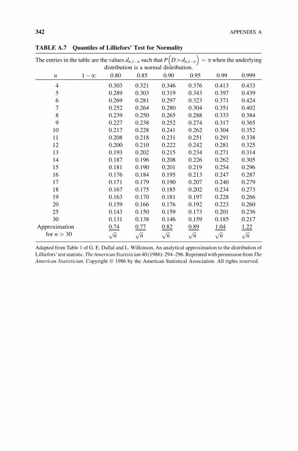
TABLE A.7 Quantiles of Lilliefors’ Test for Normality
The entries in the table are the values dn;1�a such that P DHdn;1�a
� �¼ awhen the underlying
distribution is a normal distribution.
n 1� a: 0.80 0.85 0.90 0.95 0.99 0.999
4 0.303 0.321 0.346 0.376 0.413 0.433
5 0.289 0.303 0.319 0.343 0.397 0.439
6 0.269 0.281 0.297 0.323 0.371 0.424
7 0.252 0.264 0.280 0.304 0.351 0.402
8 0.239 0.250 0.265 0.288 0.333 0.384
9 0.227 0.238 0.252 0.274 0.317 0.365
10 0.217 0.228 0.241 0.262 0.304 0.352
11 0.208 0.218 0.231 0.251 0.291 0.338
12 0.200 0.210 0.222 0.242 0.281 0.325
13 0.193 0.202 0.215 0.234 0.271 0.314
14 0.187 0.196 0.208 0.226 0.262 0.305
15 0.181 0.190 0.201 0.219 0.254 0.296
16 0.176 0.184 0.195 0.213 0.247 0.287
17 0.171 0.179 0.190 0.207 0.240 0.279
18 0.167 0.175 0.185 0.202 0.234 0.273
19 0.163 0.170 0.181 0.197 0.228 0.266
20 0.159 0.166 0.176 0.192 0.223 0.260
25 0.143 0.150 0.159 0.173 0.201 0.236
30 0.131 0.138 0.146 0.159 0.185 0.217
Approximation
for nH 30
0.74 0.77 0.82 0.89 1.04 1.22ffiffiffin
p ffiffiffin
p ffiffiffin
p ffiffiffin
p ffiffiffin
p ffiffiffin
p
Adapted from Table 1 of G. E. Dallal and L. Wilkinson, An analytical approximation to the distribution of
Lilliefors’ test statistic.TheAmerican Statistician 40 (1986): 294–296.Reprintedwith permission fromThe
American Statistician. Copyright � 1986 by the American Statistical Association. All rights reserved.
342 APPENDIX A
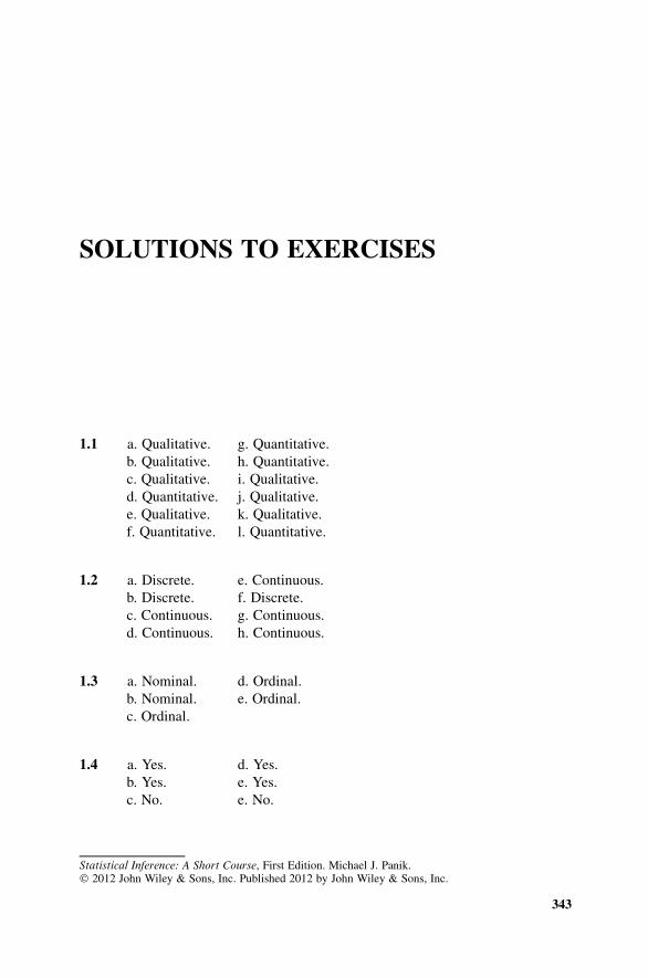
SOLUTIONS TO EXERCISES
1.1 a. Qualitative. g. Quantitative.
b. Qualitative. h. Quantitative.
c. Qualitative. i. Qualitative.
d. Quantitative. j. Qualitative.
e. Qualitative. k. Qualitative.
f. Quantitative. l. Quantitative.
1.2 a. Discrete. e. Continuous.
b. Discrete. f. Discrete.
c. Continuous. g. Continuous.
d. Continuous. h. Continuous.
1.3 a. Nominal. d. Ordinal.
b. Nominal. e. Ordinal.
c. Ordinal.
1.4 a. Yes. d. Yes.
b. Yes. e. Yes.
c. No. e. No.
Statistical Inference: A Short Course, First Edition. Michael J. Panik.� 2012 John Wiley & Sons, Inc. Published 2012 by John Wiley & Sons, Inc.
343
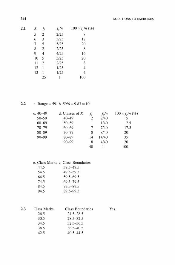
2.1 X fj fj /n 100� fj /n (%)
5 2 2/25 8
6 3 3/25 12
7 5 5/25 20
8 2 2/25 8
9 4 4/25 16
10 5 5/25 20
11 2 2/25 8
12 1 1/25 4
13 1 1/25 4
25 1 100
2.2 a. Range¼ 59. b. 59/6¼ 9.83� 10.
c. 40–49 d. Classes of X fj fj /n 100� fj /n (%)
50–59 40–49 2 2/40 5
60–69 50–59 1 1/40 2.5
70–79 60–69 7 7/40 17.5
80–89 70–79 8 8/40 20
90–99 80–89 14 14/40 35
90–99 8 4/40 20
40 1 100
e. Class Marks e. Class Boundaries
44.5 39.5–49.5
54.5 49.5–59.5
64.5 59.5–69.5
74.5 69.5–79.5
84.5 79.5–89.5
94.5 89.5–99.5
2.3 Class Marks Class Boundaries Yes.
26.5 24.5–28.5
30.5 28.5–32.5
34.5 32.5–36.5
38.5 36.5–40.5
42.5 40.5–44.5
344 SOLUTIONS TO EXERCISES
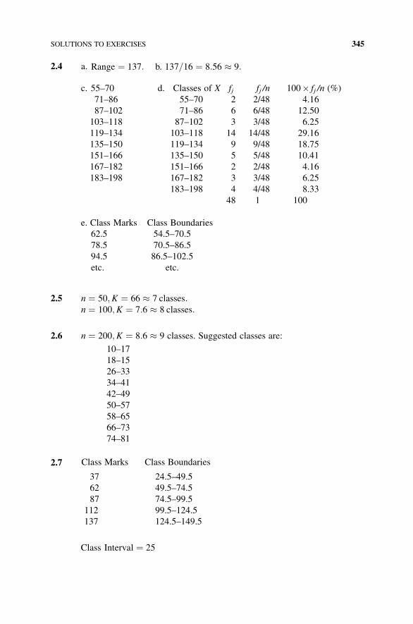
2.4 a. Range ¼ 137: b. 137=16 ¼ 8:56 � 9:
c. 55–70 d. Classes of X fj fj /n 100� fj /n (%)
71–86 55–70 2 2/48 4.16
87–102 71–86 6 6/48 12.50
103–118 87–102 3 3/48 6.25
119–134 103–118 14 14/48 29.16
135–150 119–134 9 9/48 18.75
151–166 135–150 5 5/48 10.41
167–182 151–166 2 2/48 4.16
183–198 167–182 3 3/48 6.25
183–198 4 4/48 8.33
48 1 100
e. Class Marks Class Boundaries
62.5 54.5–70.5
78.5 70.5–86.5
94.5 86.5–102.5
etc. etc.
2.5 n ¼ 50;K ¼ 66 � 7 classes:n ¼ 100;K ¼ 7:6 � 8 classes:
2.6 n ¼ 200;K ¼ 8:6 � 9 classes. Suggested classes are:
10–17
18–15
26–33
34–41
42–49
50–57
58–65
66–73
74–81
2.7 Class Marks Class Boundaries
37 24.5–49.5
62 49.5–74.5
87 74.5–99.5
112 99.5–124.5
137 124.5–149.5
Class Interval ¼ 25
SOLUTIONS TO EXERCISES 345
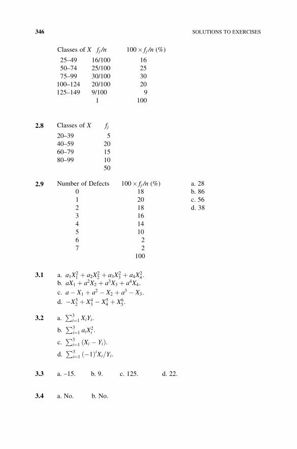
Classes of X fj /n 100� fj /n (%)
25–49 16/100 16
50–74 25/100 25
75–99 30/100 30
100–124 20/100 20
125–149 9/100 9
1 100
2.8 Classes of X fj
20–39 5
40–59 20
60–79 15
80–99 10
50
2.9 Number of Defects 100� fj /n (%) a. 28
0 18 b. 86
1 20 c. 56
2 18 d. 38
3 16
4 14
5 10
6 2
7 2
100
3.1 a. a1X21 þ a2X
22 þ a3X
23 þ a4X
24 .
b. aX1 þ a2X2 þ a3X3 þ a4X4.
c. a� X1 þ a2 � X2 þ a3 � X3.
d. �X32 þ X4
3 � X54 þ X6
5 .
3.2 a.P3
i¼1 XiYi.
b.P3
i¼1 aiX2i .
c.P3
i¼1 Xi � Yið Þ.d.
P3i¼1 �1ð ÞiXi=Yi.
3.3 a. –15. b. 9. c. 125. d. 22.
3.4 a. No. b. No.
346 SOLUTIONS TO EXERCISES
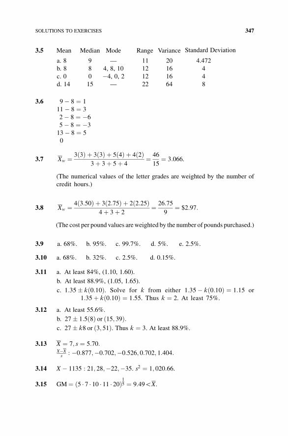
3.5 Mean Median Mode Range Variance Standard Deviation
a. 8 9 — 11 20 4.472
b. 8 8 4, 8, 10 12 16 4
c. 0 0 �4, 0, 2 12 16 4
d. 14 15 — 22 64 8
3.6 9� 8 ¼ 1
11� 8 ¼ 3
2� 8 ¼ �6
5� 8 ¼ �3
13� 8 ¼ 5
0
3.7 Xw ¼ 3ð3Þ þ 3ð3Þ þ 5ð4Þ þ 4ð2Þ3þ 3þ 5þ 4
¼ 46
15¼ 3:066.
(The numerical values of the letter grades are weighted by the number of
credit hours.)
3.8 Xw ¼ 4ð3:50Þ þ 3ð2:75Þ þ 2ð2:25Þ4þ 3þ 2
¼ 26:75
9¼ $2:97:
(The cost per pound values areweighted by the number of pounds purchased.)
3.9 a. 68%. b. 95%. c. 99.7%. d. 5%. e. 2.5%.
3.10 a. 68%. b. 32%. c. 2.5%. d. 0.15%.
3.11 a. At least 84%, (1.10, 1.60).
b. At least 88.9%, (1.05, 1.65).
c. 1:35� kð0:10Þ. Solve for k from either 1:35� kð0:10Þ ¼ 1:15 or
1:35þ kð0:10Þ ¼ 1:55. Thus k ¼ 2. At least 75%.
3.12 a. At least 55.6%.
b. 27� 1:5ð8Þ or ð15; 39Þ:c. 27� k8 or ð3; 51Þ. Thus k ¼ 3. At least 88.9%.
3.13 X ¼ 7; s ¼ 5:70:X�Xs
: �0:877;�0:702;�0:526; 0:702; 1:404:
3.14 X � 1135 : 21; 28;�22;�35. s2 ¼ 1; 020:66.
3.15 GM¼ ð5 � 7 � 10 � 11 � 20Þ15 ¼ 9:49GX.
SOLUTIONS TO EXERCISES 347
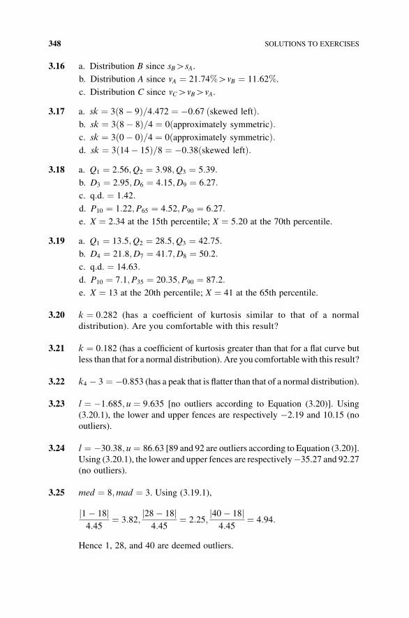
3.16 a. Distribution B since sBHsA.
b. Distribution A since vA ¼ 21:74%HvB ¼ 11:62%.
c. Distribution C since vCHvBHvA.
3.17 a. sk ¼ 3ð8� 9Þ=4:472 ¼ �0:67 ðskewed leftÞ:b. sk ¼ 3ð8� 8Þ=4 ¼ 0ðapproximately symmetricÞ:c. sk ¼ 3ð0� 0Þ=4 ¼ 0ðapproximately symmetricÞ:d. sk ¼ 3ð14� 15Þ=8 ¼ �0:38ðskewed leftÞ:
3.18 a. Q1 ¼ 2:56;Q2 ¼ 3:98;Q3 ¼ 5:39:
b. D3 ¼ 2:95;D6 ¼ 4:15;D9 ¼ 6:27:
c. q:d: ¼ 1:42:
d. P10 ¼ 1:22;P65 ¼ 4:52;P90 ¼ 6:27:
e. X ¼ 2:34 at the 15th percentile; X ¼ 5:20 at the 70th percentile.
3.19 a. Q1 ¼ 13:5;Q2 ¼ 28:5;Q3 ¼ 42:75:
b. D4 ¼ 21:8;D7 ¼ 41:7;D8 ¼ 50:2:
c. q:d: ¼ 14:63:
d. P10 ¼ 7:1;P35 ¼ 20:35;P90 ¼ 87:2:
e. X ¼ 13 at the 20th percentile; X ¼ 41 at the 65th percentile.
3.20 k ¼ 0:282 (has a coefficient of kurtosis similar to that of a normal
distribution). Are you comfortable with this result?
3.21 k ¼ 0:182 (has a coefficient of kurtosis greater than that for a flat curve but
less than that for a normal distribution). Are you comfortablewith this result?
3.22 k4 � 3 ¼ �0:853 (has a peak that is flatter than that of a normal distribution).
3.23 l ¼ �1:685; u ¼ 9:635 [no outliers according to Equation (3.20)]. Using
(3.20.1), the lower and upper fences are respectively �2.19 and 10.15 (no
outliers).
3.24 l ¼ �30:38; u ¼ 86:63 [89 and 92 are outliers according to Equation (3.20)].Using (3.20.1), the lower and upper fences are respectively�35.27 and 92.27
(no outliers).
3.25 med ¼ 8;mad ¼ 3. Using (3.19.1),
1� 18j j4:45
¼ 3:82;28� 18j j4:45
¼ 2:25;40� 18j j4:45
¼ 4:94:
Hence 1, 28, and 40 are deemed outliers.
348 SOLUTIONS TO EXERCISES
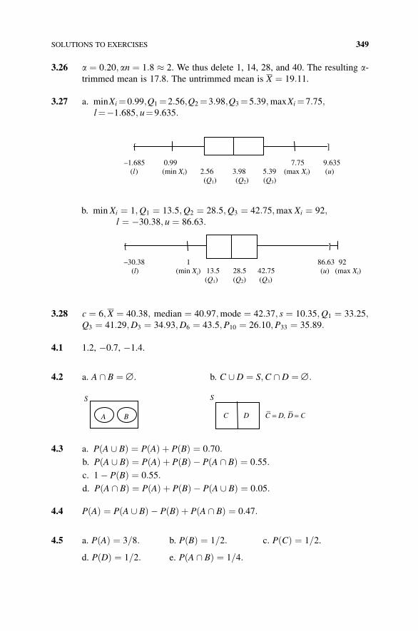
3.26 a ¼ 0:20; an ¼ 1:8 � 2. We thus delete 1, 14, 28, and 40. The resulting a-trimmed mean is 17.8. The untrimmed mean is X ¼ 19:11.
3.27 a. minXi¼0:99;Q1¼2:56;Q2¼3:98;Q3¼5:39;maxXi¼7:75;l¼�1:685; u¼9:635:
[ ]
–1.685 0.99 7.75 9.635 (l) (min Xi) 2.56 3.98 5.39 (max Xi) (u)
(Q1) (Q )2 (Q3)
b. min Xi ¼ 1;Q1 ¼ 13:5;Q2 ¼ 28:5;Q3 ¼ 42:75;max Xi ¼ 92;l ¼ �30:38; u ¼ 86:63:
[ ]
–30.38 1 86.63 92(l) (min Xi) 13.5 28.5 42.75 (u) (max Xi)
(Q1) (Q2) (Q3)
3.28 c ¼ 6;X ¼ 40:38; median ¼ 40:97;mode ¼ 42:37; s ¼ 10:35;Q1 ¼ 33:25;Q3 ¼ 41:29;D3 ¼ 34:93;D6 ¼ 43:5;P10 ¼ 26:10;P33 ¼ 35:89:
4.1 1.2, �0.7, �1.4.
4.2 a. A \ B ¼ ˘. b. C [ D ¼ S;C \ D ¼ ˘:
S
A B
S
C D C– = D, D
– = C
4.3 a. PðA [ BÞ ¼ PðAÞ þ PðBÞ ¼ 0:70:
b. PðA [ BÞ ¼ PðAÞ þ PðBÞ � PðA \ BÞ ¼ 0:55:
c. 1� PðBÞ ¼ 0:55:
d. PðA \ BÞ ¼ PðAÞ þ PðBÞ � PðA [ BÞ ¼ 0:05:
4.4 PðAÞ ¼ PðA [ BÞ � PðBÞ þ PðA \ BÞ ¼ 0:47:
4.5 a. PðAÞ ¼ 3=8: b. PðBÞ ¼ 1=2: c. PðCÞ ¼ 1=2.
d. PðDÞ ¼ 1=2: e. PðA \ BÞ ¼ 1=4:
SOLUTIONS TO EXERCISES 349
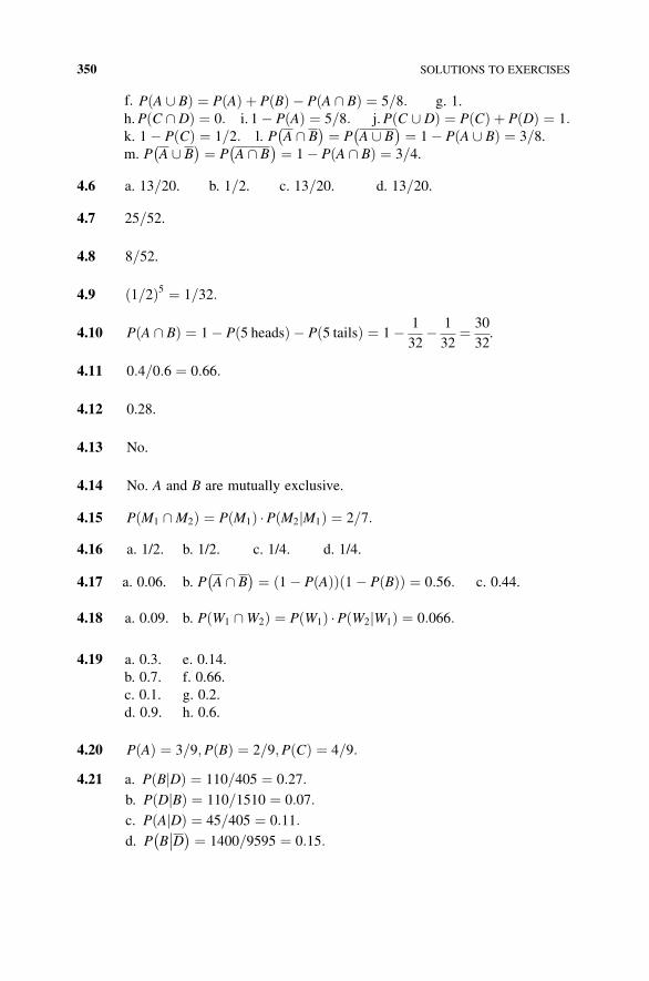
f. PðA [ BÞ ¼ PðAÞ þ PðBÞ � PðA \ BÞ ¼ 5=8: g. 1.
h.PðC \ DÞ ¼ 0: i. 1� PðAÞ ¼ 5=8: j.PðC [ DÞ ¼ PðCÞ þ PðDÞ ¼ 1:k. 1� PðCÞ ¼ 1=2: l. P A \ B
� � ¼ P A [ B� � ¼ 1� P A [ Bð Þ ¼ 3=8.
m. P A [ B� � ¼ P A \ B
� � ¼ 1� P A \ Bð Þ ¼ 3=4.
4.6 a. 13=20. b. 1=2. c. 13=20. d. 13=20.
4.7 25=52.
4.8 8=52.
4.9 ð1=2Þ5 ¼ 1=32:
4.10 PðA \ BÞ ¼ 1� Pð5 headsÞ � Pð5 tailsÞ ¼ 1� 1
32� 1
32¼ 30
32.
4.11 0:4=0:6 ¼ 0:66:
4.12 0.28.
4.13 No.
4.14 No. A and B are mutually exclusive.
4.15 P M1 \M2ð Þ ¼ P M1ð Þ �P M2 M1j Þ ¼ 2=7:ð4.16 a. 1/2. b. 1/2. c. 1/4. d. 1/4.
4.17 a. 0.06. b. P A \ B� � ¼ 1� P Að Þð Þ 1� P Bð Þð Þ ¼ 0:56: c. 0.44.
4.18 a. 0.09. b. P W1 \W2ð Þ ¼ P W1ð Þ �P W2 W1j Þ ¼ 0:066:ð
4.19 a. 0.3. e. 0.14.
b. 0.7. f. 0.66.
c. 0.1. g. 0.2.
d. 0.9. h. 0.6.
4.20 PðAÞ ¼ 3=9;PðBÞ ¼ 2=9;PðCÞ ¼ 4=9:
4.21 a. P B Dj Þ ¼ 110=405 ¼ 0:27:ðb. P D Bj Þ ¼ 110=1510 ¼ 0:07:ðc. P A Dj Þ ¼ 45=405 ¼ 0:11:ðd. P B D
�� � ¼ 1400=9595 ¼ 0:15:�
350 SOLUTIONS TO EXERCISES
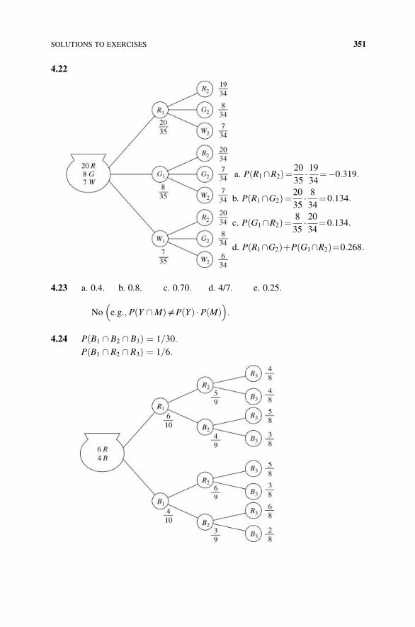
4.22
a. PðR1\R2Þ¼20
35� 1934
¼�0:319:
b. PðR1\G2Þ¼20
35� 834
¼0:134:
c. PðG1\R2Þ¼ 8
35� 2034
¼0:134:
d. P R1\G2ð ÞþP G1\R2ð Þ¼0:268:
4.23 a. 0.4. b. 0.8. c. 0.70. d. 4/7. e. 0.25.
No e:g:; P Y \Mð Þ$P Yð Þ �P Mð Þ� �
:
4.24 P B1 \ B2 \ B3ð Þ ¼ 1=30:
P B1 \ R2 \ R3ð Þ ¼ 1=6:
SOLUTIONS TO EXERCISES 351
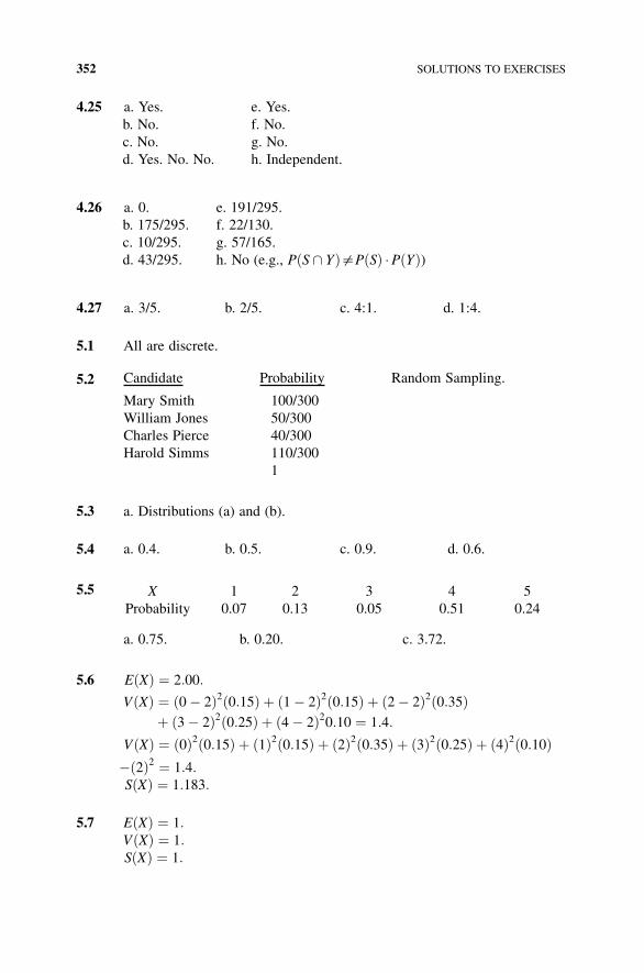
4.25 a. Yes. e. Yes.
b. No. f. No.
c. No. g. No.
d. Yes. No. No. h. Independent.
4.26 a. 0. e. 191/295.
b. 175/295. f. 22/130.
c. 10/295. g. 57/165.
d. 43/295. h. No (e.g., P S \ Yð Þ$PðSÞ �PðYÞ)
4.27 a. 3/5. b. 2/5. c. 4:1. d. 1:4.
5.1 All are discrete.
5.2 Candidate Probability Random Sampling.
Mary Smith 100/300
William Jones 50/300
Charles Pierce 40/300
Harold Simms 110/300
1
5.3 a. Distributions (a) and (b).
5.4 a. 0.4. b. 0.5. c. 0.9. d. 0.6.
5.5 X 1 2 3 4 5
Probability 0.07 0.13 0.05 0.51 0.24
a. 0.75. b. 0.20. c. 3.72.
5.6 EðXÞ ¼ 2:00:
VðXÞ ¼ ð0� 2Þ2ð0:15Þ þ ð1� 2Þ2ð0:15Þ þ ð2� 2Þ2ð0:35Þþ ð3� 2Þ2ð0:25Þ þ ð4� 2Þ20:10 ¼ 1:4:
VðXÞ ¼ ð0Þ2ð0:15Þ þ ð1Þ2ð0:15Þ þ ð2Þ2ð0:35Þ þ ð3Þ2ð0:25Þ þ ð4Þ2ð0:10Þ�ð2Þ2 ¼ 1:4:SðXÞ ¼ 1:183:
5.7 EðXÞ ¼ 1:VðXÞ ¼ 1:SðXÞ ¼ 1:
352 SOLUTIONS TO EXERCISES
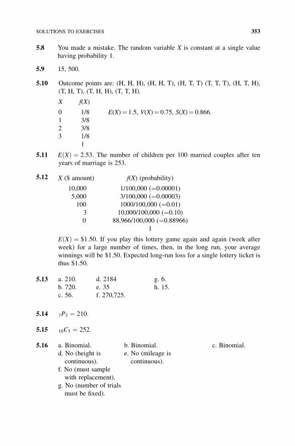
5.8 You made a mistake. The random variable X is constant at a single value
having probability 1.
5.9 15, 500.
5.10 Outcome points are: (H, H, H), (H, H, T), (H, T, T) (T, T, T), (H, T, H),
(T, H, T), (T, H, H), (T, T, H).
X f(X)
0 1/8 E(X)¼ 1.5, V(X)¼ 0.75, S(X)¼ 0.866.
1 3/8
2 3/8
3 1/8
1
5.11 EðXÞ ¼ 2:53. The number of children per 100 married couples after ten
years of marriage is 253.
5.12 X ($ amount) f(X) (probability)
10,000 1/100,000 (¼0.00001)
5,000 3/100,000 (¼0.00003)
100 1000/100,000 (¼0.01)
3 10,000/100,000 (¼0.10)
0 88,966/100,000 (¼0.88966)
1
EðXÞ ¼ $1:50. If you play this lottery game again and again (week after
week) for a large number of times, then, in the long run, your average
winnings will be $1.50. Expected long-run loss for a single lottery ticket is
thus $1.50.
5.13 a. 210. d. 2184 g. 6.
b. 720. e. 35 h. 15.
c. 56. f. 270,725.
5.14 7P3 ¼ 210:
5.15 10C5 ¼ 252:
5.16 a. Binomial. b. Binomial. c. Binomial.
d. No (height is
continuous).
e. No (mileage is
continuous).
f. No (must sample
with replacement).
g. No (number of trials
must be fixed).
SOLUTIONS TO EXERCISES 353
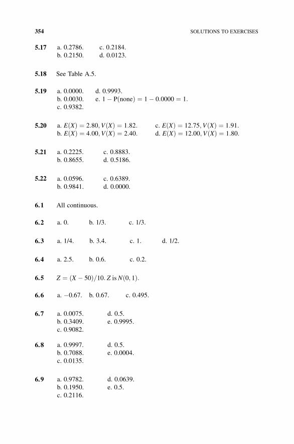
5.17 a. 0.2786. c. 0.2184.
b. 0.2150. d. 0.0123.
5.18 See Table A.5.
5.19 a. 0.0000. d. 0.9993.
b. 0.0030. e. 1� PðnoneÞ ¼ 1� 0:0000 ¼ 1:c. 0.9382.
5.20 a. EðXÞ ¼ 2:80;VðXÞ ¼ 1:82: c. EðXÞ ¼ 12:75;VðXÞ ¼ 1:91:b. EðXÞ ¼ 4:00;VðXÞ ¼ 2:40: d. EðXÞ ¼ 12:00;VðXÞ ¼ 1:80:
5.21 a. 0.2225. c. 0.8883.
b. 0.8655. d. 0.5186.
5.22 a. 0.0596. c. 0.6389.
b. 0.9841. d. 0.0000.
6.1 All continuous.
6.2 a. 0. b. 1/3. c. 1/3.
6.3 a. 1/4. b. 3.4. c. 1. d. 1/2.
6.4 a. 2.5. b. 0.6. c. 0.2.
6.5 Z ¼ ðX � 50Þ=10: Z isNð0; 1Þ:
6.6 a. �0.67. b. 0.67. c. 0.495.
6.7 a. 0.0075. d. 0.5.
b. 0.3409. e. 0.9995.
c. 0.9082.
6.8 a. 0.9997. d. 0.5.
b. 0.7088. e. 0.0004.
c. 0.0135.
6.9 a. 0.9782. d. 0.0639.
b. 0.1950. e. 0.5.
c. 0.2116.
354 SOLUTIONS TO EXERCISES
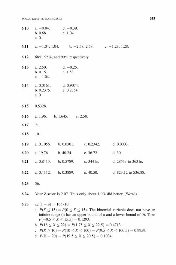
6.10 a. �0.84. d. �0.39.
b. 0.68. e. 1.04.
c. 0.
6.11 a. �1.04, 1.04. b. �2.58, 2.58. c. �1.28, 1.28.
6.12 68%, 95%, and 99% respectively.
6.13 a. 2.50. d. �0.25.
b. 0.15. e. 1.53.
c. �1.04.
6.14 a. 0.0161. d. 0.9074.
b. 0.2375. e. 0.2354.
c. 0.
6.15 0.5328.
6.16 a. 1.96. b. 1.645. c. 2.58.
6.17 71.
6.18 10.
6.19 a. 0.1056. b. 0.0301. c. 0.2342. d. 0.0003.
6.20 a. 19.76 b. 40.24. c. 36.72 d. 30.
6.21 a. 0.8413. b. 0.5789. c. 344 hr. d. 285 hr to 363 hr.
6.22 a. 0.1112. b. 0.3889. c. 40.50. d. $23.12 to $36.88.
6.23 56.
6.24 Your Z-score is 2.07. Thus only about 1.9% did better. (Wow!)
6.25 np 1� pð Þ ¼ 16H10:
a. P X � 15ð Þ ¼ P 0 � X � 15ð Þ. The binomial variable does not have an
infinite range (it has an upper bound of n and a lower bound of 0). Then
P �0:5 � X � 15:5ð Þ ¼ 0:1293:
b. P 18 � X � 22ð Þ ¼ P 1:75 � X � 22:5ð Þ ¼ 0:4713.
c. P X � 10ð Þ ¼ P 10 � X � 100ð Þ ¼ P 9:5 � X � 100:5ð Þ ¼ 0:9959.
d. P X ¼ 20ð Þ ¼ P 19:5 � X � 20:5ð Þ ¼ 0:1034:
SOLUTIONS TO EXERCISES 355
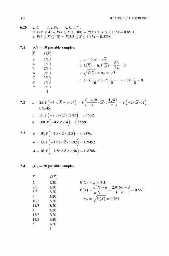
6.26 a. 6. b. 2.39. c. 0.1174.
d. PðX � 4Þ ¼ P 4 � X � 100ð Þ ¼ P 3:5 � X � 100:5ð Þ ¼ 0:8531:e. P 6 � X � 10ð Þ ¼ P 5:5 � X � 10:5ð Þ ¼ 0:5538:
7.1 5C2 ¼ 10 possible samples.
X f X� �
3 1/10 a. m ¼ 6; s ¼ ffiffiffi8
p:
4 1/10 b. E X� � ¼ 6;V X
� � ¼ 8
3
3
4¼ 3
5 2/10c.
ffiffiffiffiffiffiffiffiffiffiffiV X� �q
¼ sX ¼ ffiffiffi3
p:6 2/10
d. �3ð Þ 1
10þ �2ð Þ 1
10þ � � � þ 3ð Þ 1
10¼ 0:
7 2/10
8 1/10
9 1/10
1
7.2 n ¼ 25;P �4GX � mG4� �
¼ P�4
ffiffiffin
ps
GZG4
ffiffiffin
ps
� ¼ P �2GZG2
� �
¼ 0:9545:
n ¼ 50;P �2:82GZG2:82� �
¼ 0:9952:
n ¼ 100;P �4GZG4� �
¼ 0:9999:
7.3 s ¼ 10;P �2:5GZG2:5� �
¼ 0:9876:
s ¼ 13;P �1:92GZG1:92� �
¼ 0:9452:
s ¼ 16;P �1:56GZG1:56� �
¼ 0:8788:
7.4 6C3 ¼ 20 possible samples.
X f X� �
2 1/20 E X� � ¼ m ¼ 3:5:
7/3 1/20V X� � ¼ s2
n
N � n
N � 1¼ 2:916
3
6� 3
6� 1¼ 0:583:
8/3 2/20
sX ¼ffiffiffiffiffiffiffiffiffiffiffiV X� �q
¼ 0:764:3 3/20
10/3 3/20
11/3 3/20
4 3/20
13/3 2/20
14/3 1/20
5 1/20
1
356 SOLUTIONS TO EXERCISES
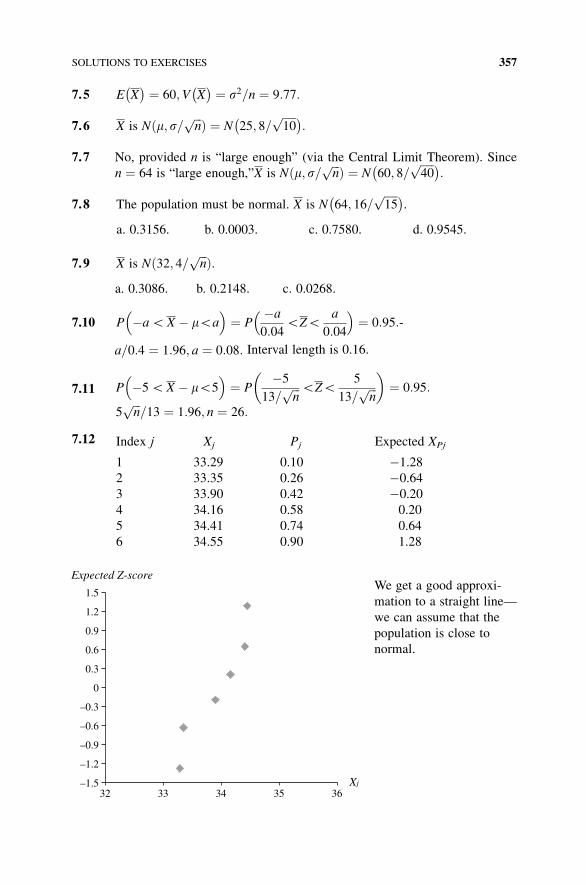
7.5 E X� � ¼ 60;V X
� � ¼ s2=n ¼ 9:77:
7.6 X is N m; s=ffiffiffin
pð Þ ¼ N 25; 8=ffiffiffiffiffi10
p� �:
7.7 No, provided n is “large enough” (via the Central Limit Theorem). Since
n ¼ 64 is “large enough,”X is N m; s=ffiffiffin
pð Þ ¼ N 60; 8=ffiffiffiffiffi40
p� �:
7.8 The population must be normal. X is N 64; 16=ffiffiffiffiffi15
p� �.
a. 0.3156. b. 0.0003. c. 0.7580. d. 0.9545.
7.9 X is N 32; 4=ffiffiffin
pð Þ.a. 0.3086. b. 0.2148. c. 0.0268.
7.10 P �aGX � mGa� �
¼ P�a
0:04GZG
a
0:04
� �¼ 0:95:-
a=0:4 ¼ 1:96; a ¼ 0:08: Interval length is 0.16.
7.11 P �5GX � mG5� �
¼ P�5
13=ffiffiffin
p GZG5
13=ffiffiffin
p�
¼ 0:95:
5ffiffiffin
p=13 ¼ 1:96; n ¼ 26:
7.12 Index j Xj Pj Expected XPj
1 33.29 0.10 �1.28
2 33.35 0.26 �0.64
3 33.90 0.42 �0.20
4 34.16 0.58 0.20
5 34.41 0.74 0.64
6 34.55 0.90 1.28
We get a good approxi-
mation to a straight line—
we can assume that the
population is close to
normal.
–1.5
–1.2
–0.9
–0.6
–0.3
0
0.3
0.6
0.9
1.2
1.5
32 33 34 35 36
Expected Z-score
Xj
SOLUTIONS TO EXERCISES 357
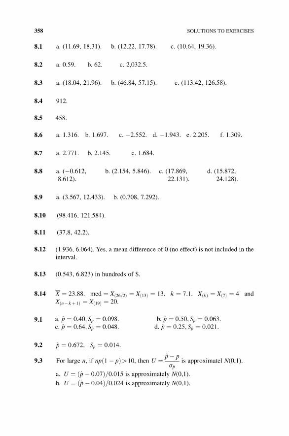
8.1 a. (11.69, 18.31). b. (12.22, 17.78). c. (10.64, 19.36).
8.2 a. 0.59. b. 62. c. 2,032.5.
8.3 a. (18.04, 21.96). b. (46.84, 57.15). c. (113.42, 126.58).
8.4 912.
8.5 458.
8.6 a. 1.316. b. 1.697. c. �2.552. d. �1.943. e. 2.205. f. 1.309.
8.7 a. 2.771. b. 2.145. c. 1.684.
8.8 a. (�0.612,
8.612).
b. (2.154, 5.846). c. (17.869,
22.131).
d. (15.872,
24.128).
8.9 a. (3.567, 12.433). b. (0.708, 7.292).
8.10 (98.416, 121.584).
8.11 (37.8, 42.2).
8.12 (1.936, 6.064). Yes, a mean difference of 0 (no effect) is not included in the
interval.
8.13 (0.543, 6.823) in hundreds of $.
8.14 X ¼ 23:88. med ¼ Xð26=2Þ ¼ Xð13Þ ¼ 13. k ¼ 7:1. XðkÞ ¼ Xð7Þ ¼ 4 and
Xðn� kþ 1Þ ¼ Xð19Þ ¼ 20.
9.1 a. p ¼ 0:40; Sp ¼ 0:098: b. p ¼ 0:50; Sp ¼ 0:063:c. p ¼ 0:64; Sp ¼ 0:048: d. p ¼ 0:25; Sp ¼ 0:021:
9.2 p ¼ 0:672; Sp ¼ 0:014:
9.3 For large n, if npð1� pÞH10, then U ¼ p� p
spis approximatel N(0,1).
a. U ¼ p� 0:07ð Þ=0:015 is approximately N(0,1).
b. U ¼ p� 0:04ð Þ=0:024 is approximately N(0,1).
358 SOLUTIONS TO EXERCISES
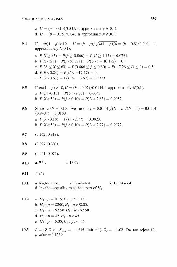
c. U ¼ p� 0:10ð Þ=0:009 is approximately N(0,1).
d. U ¼ p� 0:75ð Þ=0:043 is approximately N(0,1).
9.4 If npð1� pÞH10, U ¼ p� pð Þ= ffiffiffiffiffiffiffiffiffiffiffiffiffiffiffiffiffiffiffiffiffiffip 1� pð Þ=np ¼ p� 0:8ð Þ=0:046 is
approximately N(0,1).
a. PðX � 65Þ ¼ Pðp � 0:866Þ ¼ PðU � 1:43Þ ¼ 0:0764:
b. PðXG25Þ ¼ PðpG0:333Þ ¼ PðUG� 10:152Þ ¼ 0:
c. Pð35 � X � 60Þ ¼ Pð0:466 � p � 0:80Þ ¼ Pð�7:26 � U � 0Þ ¼ 0:5:
d. PðpG0:24Þ ¼ PðUG�12:17Þ ¼ 0:
e. PðpH0:63Þ ¼ PðUH�3:69Þ ¼ 0:9999:
9.5 If npð1� pÞH10;U ¼ ðp� 0:07Þ=0:0114 is approximately N(0,1).
a. Pð pH0:10Þ ¼ PðUH2:63Þ ¼ 0:0043:
b. PðXG50Þ ¼ PðpG0:10Þ ¼ PðUG2:63Þ ¼ 0:9957:
9.6 Since n=N ¼ 0:10, we use sp ¼ 0:0114ffiffiffiffiffiffiffiffiffiffiffiffiffiffiffiffiffiffiffiffiffiffiffiffiffiffiffiffiffiffiffiffiffiffiðN � nÞ=ðN � 1Þp ¼ 0:0114
ð0:9487Þ ¼ 0:0108:
a. PðpH0:10Þ ¼ PðUH2:77Þ ¼ 0:0028:
b. PðXG50Þ ¼ PðpG0:10Þ ¼ PðUG2:77Þ ¼ 0:9972:
9.7 (0.262, 0.318).
9.8 (0.097, 0.302).
9.9 (0.041, 0.071).
9.10 a. 971. b. 1,067.
9.11 3,959.
10.1 a. Right-tailed. b. Two-tailed. c. Left-tailed.
d. Invalid—equality must be a part of H0.
10.2 a. H0 : p ¼ 0:15;H1 : pH0:15:
b. H0 : m ¼ $200;H1 : m$$200:
c. H0 : m ¼ $2:50;H1 : mH$2:50:
d. H0 : m ¼ 85;H1 : mG85:
e. H0 : p ¼ 0:35;H1 : pH0:35:
10.3 R ¼ fZjZG�Z0:05 ¼ �1:645g left-tailð Þ: Z0 ¼ �1:02: Do not reject H0.
p-value¼ 0.1539.
SOLUTIONS TO EXERCISES 359
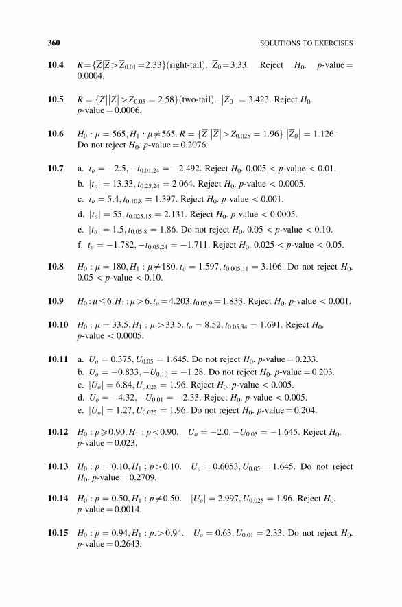
10.4 R¼fZjZHZ0:01¼2:33g right-tailð Þ: Z0¼3:33: Reject H0. p-value¼0.0004.
10.5 R ¼ fZ�� Z�� ��HZ0:05 ¼ 2:58g two-tailð Þ: Z0
�� �� ¼ 3:423: Reject H0.
p-value¼ 0.0006.
10.6 H0 : m ¼ 565;H1 : m$565: R ¼ fZ�� Z�� ��HZ0:025 ¼ 1:96g: Z0
�� �� ¼ 1:126:Do not reject H0. p-value¼ 0.2076.
10.7 a. to ¼ �2:5;�t0:01;24 ¼ �2:492: Reject H0. 0.005G p-valueG 0.01.
b. toj j ¼ 13:33; t0:25;24 ¼ 2:064: Reject H0. p-valueG 0.0005.
c. to ¼ 5:4; t0:10;8 ¼ 1:397: Reject H0. p-valueG 0.001.
d. toj j ¼ 55; t0:025;15 ¼ 2:131: Reject H0. p-valueG 0.0005.
e. toj j ¼ 1:5; t0:05;8 ¼ 1:86: Do not reject H0. 0.05G p-valueG 0.10.
f. to ¼ �1:782;�t0:05;24 ¼ �1:711: Reject H0. 0.025G p-valueG 0.05.
10.8 H0 : m ¼ 180;H1 : m$180: to ¼ 1:597; t0:005;11 ¼ 3:106: Do not reject H0.
0.05G p-valueG 0.10.
10.9 H0 :m�6;H1 :mH6:to¼4:203;t0:05;9¼1:833: Reject H0. p-valueG 0.001.
10.10 H0 : m ¼ 33:5;H1 : mH33:5: to ¼ 8:52; t0:05;34 ¼ 1:691: Reject H0.
p-valueG 0.0005.
10.11 a. Uo ¼ 0:375;U0:05 ¼ 1:645: Do not reject H0. p-value¼ 0.233.
b. Uo ¼ �0:833;�U0:10 ¼ �1:28: Do not reject H0. p-value¼ 0.203.
c. Uoj j ¼ 6:84;U0:025 ¼ 1:96: Reject H0. p-valueG 0.005.
d. Uo ¼ �4:32;�U0:01 ¼ �2:33: Reject H0. p-valueG 0.005.
e. Uoj j ¼ 1:27;U0:025 ¼ 1:96: Do not reject H0. p-value¼ 0.204.
10.12 H0 : pX0:90;H1 : pG0:90: Uo ¼ �2:0;�U0:05 ¼ �1:645: Reject H0.
p-value¼ 0.023.
10.13 H0 : p ¼ 0:10;H1 : pH0:10: Uo ¼ 0:6053;U0:05 ¼ 1:645: Do not reject
H0. p-value¼ 0.2709.
10.14 H0 : p ¼ 0:50;H1 : p$0:50: Uoj j ¼ 2:997;U0:025 ¼ 1:96: Reject H0.
p-value¼ 0.0014.
10.15 H0 : p ¼ 0:94;H1 : p:H0:94: Uo ¼ 0:63;U0:01 ¼ 2:33: Do not reject H0.
p-value¼ 0.2643.
360 SOLUTIONS TO EXERCISES
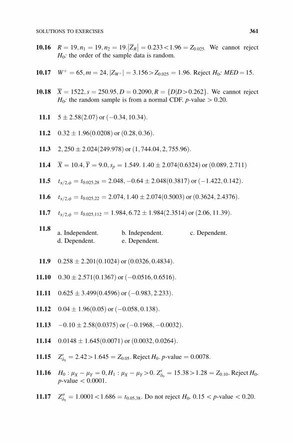
10.16 R ¼ 19; n1 ¼ 19; n2 ¼ 19: ZR
�� �� ¼ 0:233G1:96 ¼ Z0:025: We cannot reject
H0: the order of the sample data is random.
10.17 Wþ ¼ 65;m ¼ 24; ZWþj j ¼ 3:156HZ0:025 ¼ 1:96: Reject H0: MED¼ 15.
10.18 X ¼ 1522; s ¼ 250:95;D ¼ 0:2090;R ¼ fDjDH0:262g: We cannot reject
H0: the random sample is from a normal CDF. p-valueH 0.20.
11.1 5� 2:58ð2:07Þ or ð�0:34; 10:34Þ:
11.2 0:32� 1:96ð0:0208Þ or ð0:28; 0:36Þ:
11.3 2; 250� 2:024ð249:978Þ or ð1; 744:04; 2; 755:96Þ:
11.4 X ¼ 10:4; Y ¼ 9:0; sp ¼ 1:549: 1:40� 2:074ð0:6324Þ or ð0:089; 2:711Þ
11.5 ta=2;f ¼ t0:025;28 ¼ 2:048;�0:64� 2:048ð0:3817Þ or ð�1:422; 0:142Þ:
11.6 ta=2;f ¼ t0:025;22 ¼ 2:074; 1:40� 2:074ð0:5003Þ or ð0:3624; 2:4376Þ:
11.7 ta=2;f ¼ t0:025;112 ¼ 1:984; 6:72� 1:984ð2:3514Þ or ð2:06; 11:39Þ:
11.8a. Independent. b. Independent. c. Dependent.
d. Dependent. e. Dependent.
11.9 0:258� 2:201ð0:1024Þ or ð0:0326; 0:4834Þ:
11.10 0:30� 2:571ð0:1367Þ or ð�0:0516; 0:6516Þ:
11.11 0:625� 3:499ð0:4596Þ or ð�0:983; 2:233Þ:
11.12 0:04� 1:96ð0:05Þ or ð�0:058; 0:138Þ:
11.13 �0:10� 2:58ð0:0375Þ or ð�0:1968;�0:0032Þ:
11.14 0:0148� 1:645ð0:0071Þ or ð0:0032; 0:0264Þ:
11.15 Z 0d0 ¼ 2:42H1:645 ¼ Z0:05: RejectH0: p-value ¼ 0:0078:
11.16 H0 : mX � mY ¼ 0;H1 : mX � mYH0: Z 0d0 ¼ 15:38H1:28 ¼ Z0:10. RejectH0.
p-valueG 0.0001.
11.17 Z 00d0 ¼ 1:0001G1:686 ¼ t0:05;38: Do not reject H0. 0.15G p-valueG 0.20.
SOLUTIONS TO EXERCISES 361
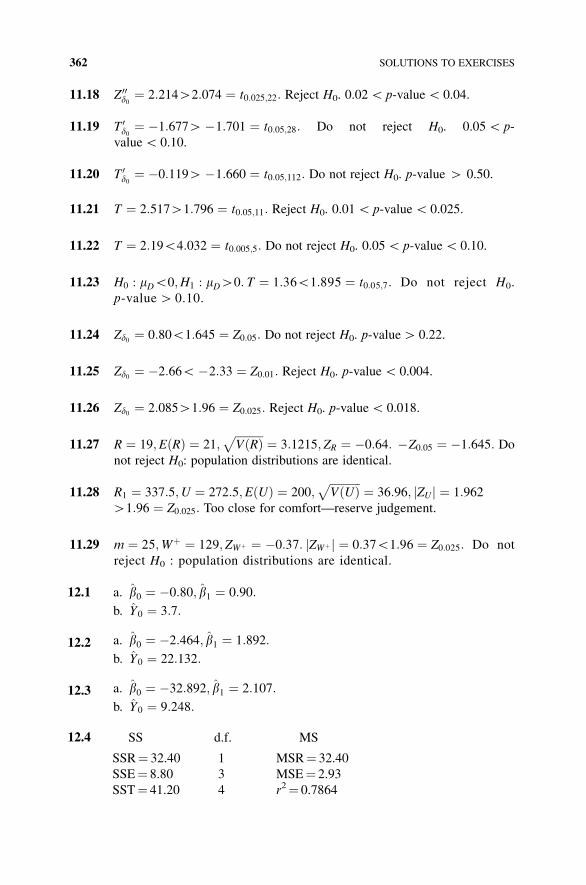
11.18 Z 00d0 ¼ 2:214H2:074 ¼ t0:025;22: Reject H0. 0.02G p-valueG 0.04.
11.19 T 0d0 ¼ �1:677H�1:701 ¼ t0:05;28: Do not reject H0. 0.05G p-
valueG 0.10.
11.20 T 0d0 ¼ �0:119H�1:660 ¼ t0:05;112: Do not reject H0. p-value H 0.50.
11.21 T ¼ 2:517H1:796 ¼ t0:05;11: Reject H0. 0.01G p-valueG 0.025.
11.22 T ¼ 2:19G4:032 ¼ t0:005;5: Do not reject H0. 0.05G p-valueG 0.10.
11.23 H0 : mDG0;H1 : mDH0: T ¼ 1:36G1:895 ¼ t0:05;7: Do not reject H0.
p-valueH 0.10.
11.24 Zd0 ¼ 0:80G1:645 ¼ Z0:05: Do not reject H0. p-valueH 0.22.
11.25 Zd0 ¼ �2:66G�2:33 ¼ Z0:01: Reject H0. p-valueG 0.004.
11.26 Zd0 ¼ 2:085H1:96 ¼ Z0:025: Reject H0. p-valueG 0.018.
11.27 R ¼ 19;E Rð Þ ¼ 21;ffiffiffiffiffiffiffiffiffiffiV Rð Þp ¼ 3:1215; ZR ¼ �0:64: �Z0:05 ¼ �1:645: Do
not reject H0: population distributions are identical.
11.28 R1 ¼ 337:5;U ¼ 272:5;E Uð Þ ¼ 200;ffiffiffiffiffiffiffiffiffiffiffiV Uð Þp ¼ 36:96; ZUj j ¼ 1:962
H1:96 ¼ Z0:025: Too close for comfort—reserve judgement.
11.29 m ¼ 25;Wþ ¼ 129; ZWþ ¼ �0:37: ZWþj j ¼ 0:37G1:96 ¼ Z0:025: Do not
reject H0 : population distributions are identical.
12.1 a. b0 ¼ �0:80; b1 ¼ 0:90:
b. Y0 ¼ 3:7:
12.2 a. b0 ¼ �2:464; b1 ¼ 1:892:
b. Y0 ¼ 22:132:
12.3 a. b0 ¼ �32:892; b1 ¼ 2:107:
b. Y0 ¼ 9:248:
12.4 SS d.f. MS
SSR¼ 32.40 1 MSR¼ 32.40
SSE¼ 8.80 3 MSE¼ 2.93
SST¼ 41.20 4 r2¼ 0.7864
362 SOLUTIONS TO EXERCISES
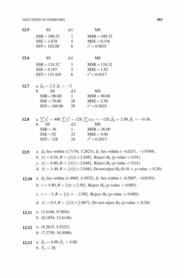
12.5 SS d.f. MS
SSR¼ 100.32 1 MSR¼ 100.32
SSE¼ 1.678 5 MSE¼ 0.336
SST¼ 102.00 6 r2¼ 0.9835
12.6 SS d.f. MS
SSR¼ 124.32 1 MSR¼ 124.32
SSE¼ 9.107 5 MSE¼ 1.82
SST¼ 133.429 6 r2¼ 0.9317
12.7 a. b0 ¼ 2:5; b1 ¼ �3:b. SS d.f. MS
SSR¼ 90.00 1 MSR¼ 90.00
SSE¼ 70.00 28 MSE¼ 2.50
SST¼ 160.00 29 r2¼ 0.5625
12.8 a.P
x2i ¼ 400;P
y2i ¼ 128;P
xiyi ¼ �120; b0 ¼ 2:90; b1 ¼ �0:30:b. SS d.f. MS
SSR¼ 36 1 MSR¼ 36.00
SSE¼ 92 23 MSE¼ 4.00
SST¼ 128 24 r2¼ 0.2813
12.9 a. b0 lies within (1.7176, 3.2823); b1 lies within (�4.0231, �1.9769).
b. tj j ¼ 6:54;R ¼ tf j tj jH2:048g. Reject H0 (p-valueG 0.01).
c. tj j ¼ 6:00;R ¼ tf j tj jH2:048g. Reject H0 (p-valueG 0.01).
d. tj j ¼ 1:40;R ¼ tf j tj jH2:048g. Do not rejectH0 (0.10G p-valueG 0.20).
12.10 a. b0 lies within (1.4965, 4.3035); b1 lies within (�0.5807, �0.0193).
b. t ¼ 5:80;R ¼ ftjtH2:50g. Reject H0 (p-valueG 0.005).
c. t ¼ �3;R ¼ ftjtH�2:50g. Reject H0 (p-valueG 0.005).
d. tj j ¼ 0:5;R ¼ tf j tj jH2:807g. Do not reject H0 (p-valueG 0.20).
12.11 a. (3.4146, 9.3854).
b. (0.1854, 12.6146).
12.12 a. (8.2635, 9.5223).
b. (7.2759, 10.5098).
12.13 a. b0 ¼ 4:00; b1 ¼ 4:00:
b. Yo ¼ 28:
SOLUTIONS TO EXERCISES 363
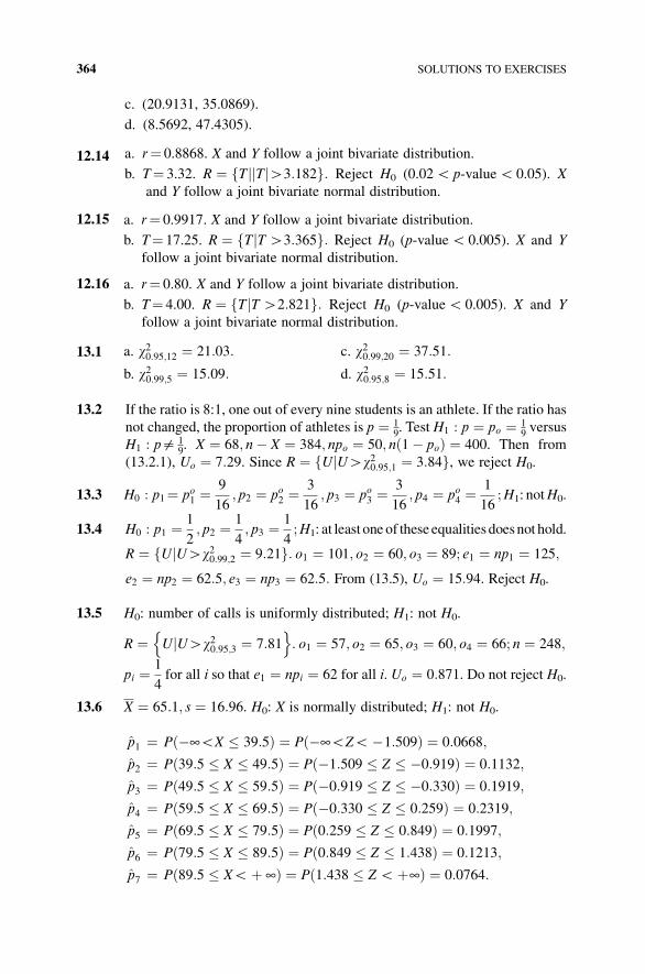
c. (20.9131, 35.0869).
d. (8.5692, 47.4305).
12.14 a. r¼ 0.8868. X and Y follow a joint bivariate distribution.
b. T¼ 3.32. R ¼ Tf j Tj jH3:182g: Reject H0 (0.02G p-valueG 0.05). X
and Y follow a joint bivariate normal distribution.
12.15 a. r¼ 0.9917. X and Y follow a joint bivariate distribution.
b. T¼ 17.25. R ¼ Tf jT H3:365g: Reject H0 (p-valueG 0.005). X and Y
follow a joint bivariate normal distribution.
12.16 a. r¼ 0.80. X and Y follow a joint bivariate distribution.
b. T¼ 4.00. R ¼ Tf jT H2:821g: Reject H0 (p-valueG 0.005). X and Y
follow a joint bivariate normal distribution.
13.1 a. w20:95;12 ¼ 21:03: c. w20:99;20 ¼ 37:51:
b. w20:99;5 ¼ 15:09: d. w20:95;8 ¼ 15:51:
13.2 If the ratio is 8:1, one out of every nine students is an athlete. If the ratio has
not changed, the proportion of athletes is p ¼ 19. Test H1 : p ¼ po ¼ 1
9versus
H1 : p$ 19. X ¼ 68; n� X ¼ 384; npo ¼ 50; nð1� poÞ ¼ 400. Then from
(13.2.1), Uo ¼ 7:29. Since R ¼ fUjUHw20:95;1 ¼ 3:84g, we reject H0.
13.3 H0 : p1¼ po1 ¼9
16; p2 ¼ po2 ¼
3
16; p3 ¼ po3 ¼
3
16; p4 ¼ po4 ¼
1
16;H1: notH0.
13.4 H0 : p1 ¼ 1
2; p2 ¼ 1
4; p3 ¼ 1
4;H1: at least one of these equalities doesnot hold.
R ¼ fUjUHw20:99;2 ¼ 9:21g: o1 ¼ 101; o2 ¼ 60; o3 ¼ 89; e1 ¼ np1 ¼ 125;
e2 ¼ np2 ¼ 62:5; e3 ¼ np3 ¼ 62:5: From (13.5), Uo ¼ 15:94. Reject H0.
13.5 H0: number of calls is uniformly distributed; H1: not H0.
R ¼ UjUHw20:95;3 ¼ 7:81n o
: o1 ¼ 57; o2 ¼ 65; o3 ¼ 60; o4 ¼ 66; n ¼ 248;
pi ¼ 1
4for all i so that e1 ¼ npi ¼ 62 for all i. Uo ¼ 0:871. Do not reject H0.
13.6 X ¼ 65:1; s ¼ 16:96. H0: X is normally distributed; H1: not H0.
p1 ¼ Pð�¥GX � 39:5Þ ¼ Pð�¥GZG�1:509Þ ¼ 0:0668;
p2 ¼ P 39:5 � X � 49:5ð Þ ¼ P �1:509 � Z � �0:919ð Þ ¼ 0:1132;
p3 ¼ P 49:5 � X � 59:5ð Þ ¼ P �0:919 � Z � �0:330ð Þ ¼ 0:1919;
p4 ¼ P 59:5 � X � 69:5ð Þ ¼ P �0:330 � Z � 0:259ð Þ ¼ 0:2319;
p5 ¼ P 69:5 � X � 79:5ð Þ ¼ P 0:259 � Z � 0:849ð Þ ¼ 0:1997;
p6 ¼ P 79:5 � X � 89:5ð Þ ¼ P 0:849 � Z � 1:438ð Þ ¼ 0:1213;
p7 ¼ Pð89:5 � XGþ ¥Þ ¼ Pð1:438 � ZGþ¥Þ ¼ 0:0764:
364 SOLUTIONS TO EXERCISES
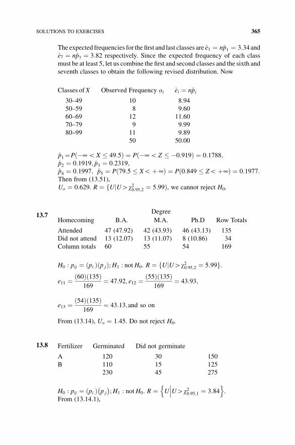
The expected frequencies for the first and last classes are e1 ¼ np1 ¼ 3:34 ande7 ¼ np7 ¼ 3:82 respectively. Since the expected frequency of each class
must be at least 5, let us combine the first and second classes and the sixth and
seventh classes to obtain the following revised distribution. Now
Classes ofX Observed Frequency oi ei ¼ npi
30–49 10 8.94
50–59 8 9.60
60–69 12 11.60
70–79 9 9.99
80–99 11 9.89
50 50.00
p1¼Pð�¥GX � 49:5Þ ¼ Pð�¥G Z � �0:919Þ ¼ 0:1788;p2 ¼ 0:1919; p3 ¼ 0:2319;p4 ¼ 0:1997; p5 ¼ Pð79:5 � XGþ ¥Þ ¼ Pð0:849 � ZGþ¥Þ ¼ 0:1977:Then from (13.51),
Uo ¼ 0:629. R ¼ fUjUHw20:95;2 ¼ 5:99Þ, we cannot reject H0.
13.7Degree
Homecoming B.A. M.A. Ph.D Row Totals
Attended 47 (47.92) 42 (43.93) 46 (43.13) 135
Did not attend 13 (12.07) 13 (11.07) 8 (10.86) 34
Column totals 60 55 54 169
H0 : pij ¼ ðpi:Þðp:jÞ;H1 : notH0: R ¼ fUjUHw20:95;2 ¼ 5:99g.
e11 ¼ 60ð Þ 135ð Þ169
¼ 47:92; e12 ¼ 55ð Þ 135ð Þ169
¼ 43:93;
e13 ¼ 54ð Þ 135ð Þ169
¼ 43:13;and so on
From (13.14), Uo ¼ 1:45. Do not reject H0.
13.8 Fertilizer Germinated Did not germinate
A 120 30 150
B 110 15 125
230 45 275
H0 : pij ¼ pi:ð Þ p:j� �
;H1 : notH0: R ¼ U UHw20:95;1 ¼ 3:84���
on.
From (13.14.1),
SOLUTIONS TO EXERCISES 365
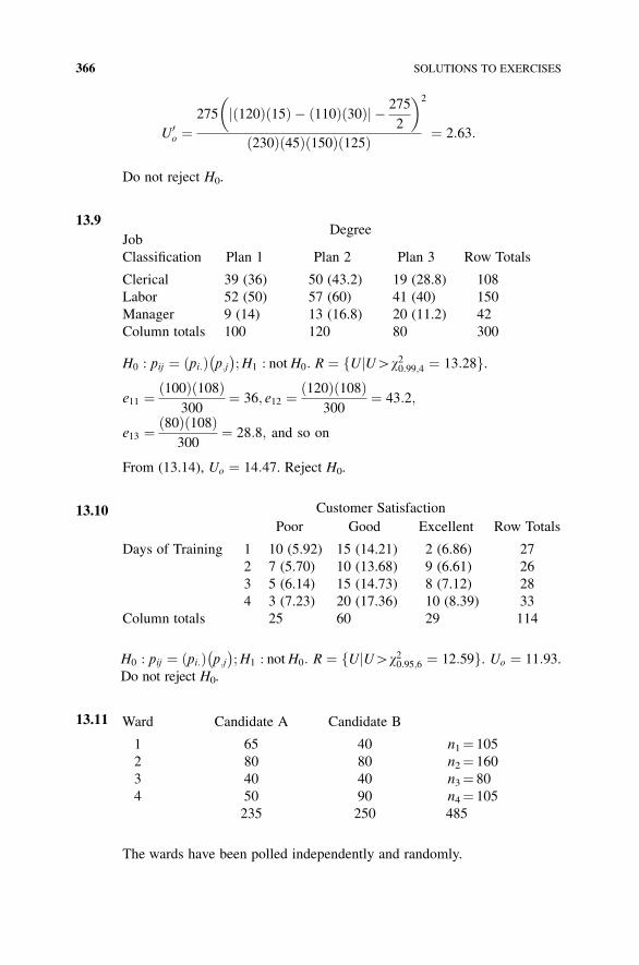
U0o ¼
275 120ð Þ 15ð Þ � 110ð Þ 30ð Þj j � 275
2
�
230ð Þ 45ð Þ 150ð Þ 125ð Þ
2
¼ 2:63:
Do not reject H0.
13.9Degree
Job
Classification Plan 1 Plan 2 Plan 3 Row Totals
Clerical 39 (36) 50 (43.2) 19 (28.8) 108
Labor 52 (50) 57 (60) 41 (40) 150
Manager 9 (14) 13 (16.8) 20 (11.2) 42
Column totals 100 120 80 300
H0 : pij ¼ pi:ð Þ p:j� �
;H1 : not H0: R ¼ fUjUHw20:99;4 ¼ 13:28g.
e11 ¼ 100ð Þ 108ð Þ300
¼ 36; e12 ¼ 120ð Þ 108ð Þ300
¼ 43:2;
e13 ¼ 80ð Þ 108ð Þ300
¼ 28:8; and so on
From (13.14), Uo ¼ 14:47. Reject H0.
13.10 Customer Satisfaction
Poor Good Excellent Row Totals
Days of Training 1 10 (5.92) 15 (14.21) 2 (6.86) 27
2 7 (5.70) 10 (13.68) 9 (6.61) 26
3 5 (6.14) 15 (14.73) 8 (7.12) 28
4 3 (7.23) 20 (17.36) 10 (8.39) 33
Column totals 25 60 29 114
H0 : pij ¼ pi:ð Þ p:j� �
;H1 : notH0: R ¼ fUjUHw20:95;6 ¼ 12:59g. Uo ¼ 11:93.Do not reject H0.
13.11 Ward Candidate A Candidate B
1 65 40 n1¼ 105
2 80 80 n2¼ 160
3 40 40 n3¼ 80
4 50 90 n4¼ 105
235 250 485
The wards have been polled independently and randomly.
366 SOLUTIONS TO EXERCISES
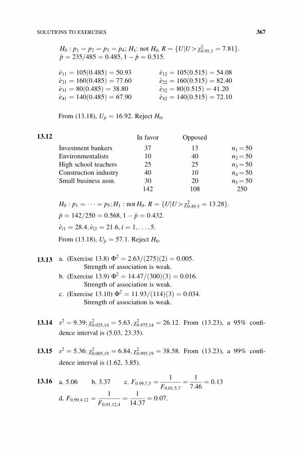
H0 : p1 ¼ p2 ¼ p3 ¼ p4; H1: not H0. R ¼ fUjUHw20:95;3 ¼ 7:81g.p ¼ 235=485 ¼ 0:485; 1� p ¼ 0:515:
e11 ¼ 105ð0:485Þ ¼ 50:93 e12 ¼ 105ð0:515Þ ¼ 54:08e21 ¼ 160ð0:485Þ ¼ 77:60 e22 ¼ 160ð0:515Þ ¼ 82:40e31 ¼ 80ð0:485Þ ¼ 38:80 e32 ¼ 80ð0:515Þ ¼ 41:20e41 ¼ 140ð0:485Þ ¼ 67:90 e42 ¼ 140ð0:515Þ ¼ 72:10
From (13.18), Up ¼ 16:92. Reject H0.
13.12 In favor Opposed
Investment bankers 37 13 n1¼ 50
Environmentalists 10 40 n2¼ 50
High school teachers 25 25 n3¼ 50
Construction industry 40 10 n4¼ 50
Small business assn. 30 20 n5¼ 50
142 108 250
H0 : p1 ¼ � � � ¼ p5;H1 : notH0. R ¼ fUjUHw20:49;3 ¼ 13:28g.p ¼ 142=250 ¼ 0:568; 1� p ¼ 0:432:
ei1 ¼ 28:4; ei2 ¼ 21:6; i ¼ 1; . . . ; 5:
From (13.18), Up ¼ 57:1. Reject H0.
13.13 a. (Exercise 13.8) F2 ¼ 2:63=ð275Þð2Þ ¼ 0:005:Strength of association is weak.
b. (Exercise 13.9) F2 ¼ 14:47=ð300Þð3Þ ¼ 0:016:Strength of association is weak.
c. (Exercise 13.10) F2 ¼ 11:93=ð114Þð3Þ ¼ 0:034:Strength of association is weak.
13.14 s2 ¼ 9:39; w20:025;14 ¼ 5:63; w20:975;14 ¼ 26:12. From (13.23), a 95% confi-
dence interval is (5.03, 23.35).
13.15 s2 ¼ 5:36; w20:005;19 ¼ 6:84; w20:995;19 ¼ 38:58. From (13.23), a 99% confi-
dence interval is (1.62, 3.85).
13.16 a. 5.06 b. 3.37 c. F0:99;7;5 ¼ 1
F0:01;5;7¼ 1
7:46¼ 0:13
d. F0:99;4;12 ¼ 1
F0:01;12;4¼ 1
14:37¼ 0:07.
SOLUTIONS TO EXERCISES 367
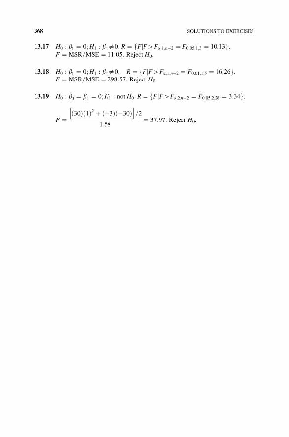
13.17 H0 : b1 ¼ 0;H1 : b1$0: R ¼ fFjFHFa;1;n�2 ¼ F0:05;1;3 ¼ 10:13g.F ¼ MSR=MSE ¼ 11:05. Reject H0.
13.18 H0 : b1 ¼ 0;H1 : b1$0: R ¼ fFjFHFa;1;n�2 ¼ F0:01;1;5 ¼ 16:26g.F ¼ MSR=MSE ¼ 298:57. Reject H0.
13.19 H0 : b0 ¼ b1 ¼ 0;H1 : notH0: R ¼ fFjFHFa;2;n�2 ¼ F0:05;2;28 ¼ 3:34g.
F ¼30ð Þ 1ð Þ2 þ �3ð Þ �30ð Þ
h i=2
1:58¼ 37:97. Reject H0.
368 SOLUTIONS TO EXERCISES

REFERENCES
Anderson, J., Brown, R., Risk and Insurance P-21-05, 2nd printing: Society of Actuaries,
(2005).
Aristotle, Metaphysics, trans. byW. D. Ross, in The BasicWorks of Aristotle (RichardM., ed.).
New York: Random House, (1941).
Aristotle, Posterior Analytics, trans. by E. S. Bouchier in Aristotle’s Posterior Analytics.
Oxford: Blackwell, (1901).
Austin, P. C., A Critical Appraisal of Propensity—Score Matching in the Medical Literature
from 1996 to 2003. Statistics in Medicine 27: 2037–2049, (2008).
Beltrami, E., What is Random? New York: Springer-Verlag, Inc., (1999).
Blom, G., Statistical Estimates and Transformed Beta-Variables. New York: John Wiley and
Sons, (1958).
Cole, P., Causality in Epidemiology, Health Policy, and Law. Journal of Marketing Research
27: 10279–10285, (1997).
Collier, D., Sekhon, J., Stark, J., Statistical Models and Causal Inference. New York:
Cambridge University Press, (2010).
Croucher, John S., Cause and Effect in Law, Medicine, Business, and Other Fields. Review of
Business Research 8(6): 67–71, (2008).
David, Philip, Seeing and Doing: The Pearlian Synthesis. In: Heuristics, Probability, and
Causality (Dechter, R., Geffner, H. Halpern, J., eds.). New York: Cambridge University
Press, (2010).
Dechter, R., Geffner, H., Halpern, J., eds., Heuristics, Probability, and Causality. London:
College Publications, (2010).
Finkelstein, M. O., Levin, B., Statistics for Lawyers. New York: Springer-Verlag, (1990).
Statistical Inference: A Short Course, First Edition. Michael J. Panik.� 2012 John Wiley & Sons, Inc. Published 2012 by John Wiley & Sons, Inc.
369

Freedman, D., Statistical Models and Shoe Leather. Sociological Methodology 21: 291–313
(Marsden, P. V., ed.). Washington, D.C.: American Sociological Association, (1991).
Freedman, D., From Association to Causation: Some Remarks on the History of Statistics.
Statistical Science 14: 243–258, (1999).
Freedman, D., Statistical Models and Causal Inference. (Collier, D., Sekhon, J., Stark, J.,
eds.). New York: Cambridge University Press, (2010).
Freedman, D., Stark, P. B., The Swine FluVaccine andGuillian-Barre Syndrome: ACase Study
in Relative Risk and Specific Causation. Evaluation Review 23: 619–647, (1999).
Glymour, M. M., Greenland, S., Causal Diagrams. In:Modern Epidemiology (Rothman, K. J.,
Greenland, S. Lash, T. L., eds.). Philadelphia: Lippincott, Williams & Wilkins, (2008).
Godfrey-Smith, P., Theory and Reality: An Introduction to the Philosophy of Science. Chicago:
University of Chicago Press, (2003).
Greenland, S., Confounding. In: Encyclopedia of Biostatistics (Armitage, P., Colton, T., eds.).
New York: John Wiley & Sons, (1998).
Greenland, S., Brumback, B., An Overview of Relations Among Causal Modelling Methods.
International Journal of Epidemiology 31: 1030–1037, (2002).
Holland, P. M., Statistics and Causal Inference (with discussion). Journal of the American
Statistical Association 81: 945–971, (1986).
Hull, T. E., Dobell, A. R., Random Number Generators. SIAM Review 4: 230–254, (1962).
Humphreys, P., The Chances of Explanation: Causal Explanations in the Social, Medical, and
Physical Sciences. Princeton: Princeton University Press, (1997).
Humphreys, P., Extending Ourselves: Computational Science, Empiricism, and Scientific
Method. New York: Oxford University Press, (2004).
Knight, F., Risk, Uncertainty, and Profit. New York: Harper, (1921).
Lorenz, E., Predictability: Does the Flap of a Butterfly’s Wings in Brazil Set Off a
Tornado in Texas? Address given at the American Assn. for the Advancement of
Science, (1972).
Morgan, S., Winship, C., Counterfactuals and Causal Inference, 7th printing. New York:
Cambridge University Press, (2010).
Pearl, J., Embracing Causality in Formal Reasoning. Artificial Intelligence 35(2): 259–271,
(1988).
Pearl, J., Causality, 2nd ed., New York: Cambridge University Press, (2009).
Psillos, S., Scientific Realism: How Science Tracks Truth. London: Routledge, (1999).
Rao, C. R., Statistics and Truth, 2nd ed., London: World Scientific Publishing Co. (1997).
Rubin, D. B., Estimating Causal Effects of Treatments in Randomized and Non-randomized
Studies. Journal of Education Psychology 66: 688–701, (1974).
Rubin, D. B., Assignment of Treatment Groups on the Basis of a Covariate. Journal of
Educations Statistics 2: 1–26, (1977).
Rubin, D. B., Bayesian Inference for Causal Effects: TheRole of Randomization. TheAnnals of
Statistics 6: 34–58, (1978).
Rubin, D. B., Discussion of Randomization Analysis of Experimental Data: The Fisher
Randomization Test, by D. Basu, Journal of the American Statistical Association 75:
591–593, (1980).
370 REFERENCES

Rubin, D. B., The Design Versus the Analysis of Observational Studies for Causal Effects:
Parallels with the Design of Randomized Trials. Statistics in Medicine 26: 20–36,
(2007).
Snow, J. (1855), On the Mode of Communication of Cholera, Reprinted ed. New York:
Hafner, (1965).
Tsonis, A., Randomnicity. London: Imperial College Press, (2008).
371
INDEX
Absolute value function, 35, 101
Accuracy, 158
A posteriori, 73
A priori, 73
Asymptotic, 102
Axiom, 65
Bernoulli probability distribution, 91
Binomial probability distribution, 91
binomial probability, 92
table of cumulative values, 338–341
table of values, 334–337
Boxplot, 42
whiskers, 42
Butterfly effect, 146
Lorenz, E., 145
Causality
average effect, 291
causal, 287
cause, 291
counterfactual, 289
effect, 292
fundamental problem, 290
intervention principle, 291
lurking variable, 288–289
necessary cause, 286
post-exposure values, 290–291
spurious correlation, 288–289
statistical, 287
sufficient cause, 286
Cell frequencies, 296, 299
expected, 299, 310
observed, 296, 307, 310
Central limit theorem, 130
Chaos, 143, 145
Chebysheff’s theorem, 30
Chi-square
distribution, 298
table of values, 327–328
Class
boundary, 14
deviation, 53
frequency, 12
interval, 12, 53
limits, 14
mark, 14
modal, 55
Statistical Inference: A Short Course, First Edition. Michael J. Panik.� 2012 John Wiley & Sons, Inc. Published 2012 by John Wiley & Sons, Inc.
373
Coefficient of determination, 264
Combination, 90
Confidence coefficient, 157
Confidence interval
confidence probability, 154, 174
for difference of means, 217–224
for difference of proportions, 227–228
for mean, 156, 183
for median, 167
for proportion, 175
for ratio, 181
for standard deviation, 314
for variance, 314
paired comparisons, 224–227
percentage points, 155, 161
reliability, 157, 176
Contingency table, 304
estimated probability, 306
marginal probability, 306
marginal totals, 305
Correlation coefficient
goodness of fit, 277–278
inferences about, 275–277
population, 273
sample, 274
Cramer’s phi-squared, 312
Cumulative distribution function, 83, 213
empirical, 213
Data
bivatiate, 253
interval, 5
metric, 5
nominal, 4
nonmetric, 5
nonnumerical, 1
numerical, 1
ordinal, 4
ratio, 5
reduction, 123
univatiate, 253
Decision tree
branch, 71
node, 71
Degrees of freedom, 28, 160
Deviation from the mean, 24
Elementary sampling unit, 3
observation, 6
Empirical rule, 30, 103
Error
nonsampling, 4
sampling, 4
Error bound,
for mean, 152
for proportion, 173
Estimator, 123
biased, 29
consistent, 128
interval, 154
point, 154
unbiased, 126, 171, 172
Event(s)
certain, 65
compound, 63
equiprobable, 66
impossible, 64
independent, 70
test criterion for, 70
Expectation, 85
Experimental design
control group, 283
double blind, 283
experiment, 282
experimental group, 283
experimental study, 293
experimental unit, 283
factors, 282
interaction, 282
natural, 294
observational study, 293–294
pairing, 224
placebo, 283
randomized, 282–283
replication, 283
response, 282
treatment, 283
F distribution
percentage points, 315
table of values, 329–333
F test
joint test, 317
regression slope, 316
Finite population correction,
127, 178
Five number summary, 42
Freedman, D., 293
374 INDEX
Frequency density, 19
Frequency distribution
absolute, 9, 12, 51
cumulative, 83, 213
percent, 10, 14
relative, 10, 14
Frequency function
absolute, 11
percent, 11
relative, 11
Frequency limit principle, 73
Gambler’s fallacy, 74
Gauss-Markov theorem, 262
Goodness of fit
Pearson’s test, 295
Heavy-tailed distributions, 164
Histogram, 14
Hypothesis
alternative, 185
compound, 185
distributional, 295
maintained, 185
null, 185
parametric, 211, 295
research, 198
simple, 185
statistical, 184
Hypothesis testing
classical approach, 190
classical decision rule, 191
critical region, 190
critical value, 190
difference of means, 228–234
difference of proportions,
236–238
level of significance, 190
nonparametric test, 212
null value, 185
one-tail test, 191–192
p-value, 198
region of nonrejection, 190
reserve judgement, 196
stepwise procedure, 191
standardized value, 191, 202
test for mean, 191–197
test for median, 210
test for normality, 280, 302
test for proportion, 201–204
test for randomness, 208, 292
test statistic, 190
type I error, 185
type II error, 185
two-tail test, 193
Induction, 2
Insurance
benefit, 147
premium, 147
risk pooling, 147
Knight, F., 146
Kurtosis
coefficient of, 38
excess, 38
standard, 38
Law of large numbers, 73, 147
Least squares
normal equations, 258
principle of, 258
Lilliefors test, 213
Linear relationship
dependent variable, 254
direct, 253
exact, 254
independent variable, 254
inverse, 253
slope, 254
vertical intercept, 254
Linear translation, 49
Loss distribution
frequency of loss, 148
insurance loss, 148
severity of loss, 148
Mean
assumed, 52
geometric, 49
population, 23
sample, 23
trimmed, 41
weighted, 25
Median, 26, 53
Mode, 27,55
Mann-Whitney rank sum test,
245
INDEX 375
Nonlinear relationship, 253
Normal distribution, 30, 102
approximation to binomial, 120
continuity correction, 120
percentage points, 155, 175
percentiles, 114
standard normal, 105
table of values, 323–324
testing normality, 280, 302–304
Normal probability plot, 136
Observed relative frequency of a success, 170
standardized, 172
Odds, 79
Order statistics, 167
Outlier, 24, 39
fences for, 39, 40, 42
Parameter, 22, 300
completely specified, 300
Pearson coefficient of skewness, 35
Pearson multinomial chi-square
distribution, 297
statistic, 297, 302
test for association, 307
test for independence, 304
testing k proportions, 309
Population
sampled, 6
target, 6
Prediction
average value, 269–270
confidence interval for, 269
confidence band, 270
forecast error, 270
particular value, 270–272
confidence interval for, 271
Principle, 258
Probability
addition rule, 66
axioms, 65
classical, 66
conditional, 69
corollaries, 66
empirical, 73
joint, 69
mass function, 82
multiplication rule, 70
objective, 73
relative frequency, 73
sources, 73
subjective, 73
theoretical, 73
Probability density function, 101
Probability distribution
continuous, 101
discrete, 82
expected, 299
multinomial, 296
normal, 30, 102
population, 296
sample, 296
uniform, 82
Propositions
logical fallacy (cum hoc, ergo propter
hoc), 289
logical implications, 284
necessary condition, 285
negation, 283
sufficient condition, 285
truth sets, 283
truth table, 283
truth values, 283
Quantiles
deciles, 36
interquartile range, 37
percentiles, 36
quartile deviation, 37
quartiles, 36
Random experiment, 63, 82
multinomial, 296
Random numbers
artificially generated, 144
natural, 144
pseudo, 139
pure, 144
reversibility, 142
table of, 134
Random phenomenon, 63
Random sample, 122
sampling cycle, 135
systematic, 135
Random variable
continuous, 101
discrete, 82
mean, 85
376 INDEX
multinomial, 296
standard deviation, 86
variance, 86
Randomness, 139
types, 142
Range, 12, 27
Ratio estimate, 180
from sample, 179
Regression coefficients
confidence intervals for,
266–267
formulas for, 259
hypothesis tests for, 267–269
standard errors, 265
Regression equation
distribution assumptions, 257
population, 256
random component, 255, 257
regressor, 255
residual, 257
response variable, 255
sample, 257
statistical, 256
systematic component, 255
Risk, 146
Run, 208
Runs test, 208
two independent samples, 243
Sample
biased, 4
frame, 3
random, 3, 122
representative, 3
Sample median absolute deviation,
39
Sample size requirement
for mean, 159
for population, 176
Sample space, 63
effective, 70
Sampling
random, 3, 122
systematic, 135
with replacement, 3, 71
without replacement, 3, 72
Sampling distribution
of mean, 123
of proportion, 171
Sampling error, 124
Scatter diagram, 253
Set
collectively exhaustive, 62
complement, 62
countable, 81
countably infinite, 81
DeMorgan’s laws, 63
difference, 62
disjoint, 62
element, 61
element inclusion, 61
intersection, 62
null, 62
partition, 62
subset, 61
union, 61
unit interval, 64
universal, 62
Set function, 64
Signed ranks, 210
Skewness
left skewed, 34
right skewed, 34
standard, 36
Standard deviation, 28, 57
population, 28
sample, 28
Standard error
of mean, 128
of proportion, 171
Standard error of estimate, 265
Standardized sample
mean, 130
Standardized variable, 31
Statistical inference, 2
Statistical significance, 197
Statistics, 1
descriptive, 2
inductive, 2
Sturge’s rule, 17
Summation sign, 7
Sums of squares
error, 263
partitioned, 263–264
regression, 263
total, 263
Symmetrical distribution,
34
INDEX 377

t distribution, 160
percentage points, 161
table of values, 325–326
t statistic, 160
Testing. See hypothesis testing.
Tsonis, A., 142
Unit distribution, 32
Uncertainty, 146
Variable
continuous, 3
discrete, 3
qualitative, 2
quantitative, 3
random, 63
Variance
population, 28
sample, 28
Variation
absolute, 33
coefficient of, 34
relative, 33
Wilcoxon signed rank test, 249
paired comparisons, 249
Yates continuity correction, 308
Z-score, 32, 39
378 INDEX
![A Survey on Software-Defined Network and OpenFlow: From ... list/papers...Such an idea is defined in an innovative technology, called Software-Defined Networking (SDN) [4]. Its](https://img.pdfslide.net/doc/110x75/60e08556585db628f1249f4c/a-survey-on-software-deined-network-and-openflow-from-listpapers-such.jpg)