Embed Size (px)
Citation preview
Paola Festa - DMA, University of Napoli FEDERICO II
E-mail: [email protected] - Web: http://www.dma.unina.it/∼festaNetwork Flows - p. 1/105
Operational Research aspects in Routing:Network Flows
Paola Festa
Department of Mathematics and Applications “R. Caccioppoli”
University of Napoli FEDERICO II
http://www.dma.unina.it/∼festa/
E-mail: [email protected]
Preliminaries: notation
Network Flow Problems
Network Flows: Variants
Special cases of the
Network Flow Problem
The Maximum Flow Problem
A solution method:
the Ford-Fulkerson algorithm
A simpler (not more efficient)
implementation
of Ford-Fulkerson algorithm
Ford-Fulkerson algorithm:
an exercise
Paola Festa - DMA, University of Napoli FEDERICO II
E-mail: [email protected] - Web: http://www.dma.unina.it/∼festaNetwork Flows - p. 2/105
Preliminaries: notation
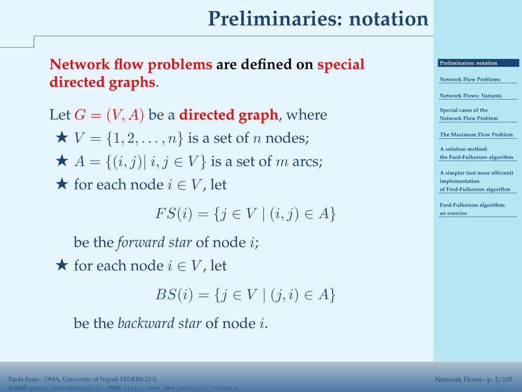
Network flow problems are defined on specialdirected graphs.
Let G = (V,A) be a directed graph, where
★ V = {1, 2, . . . , n} is a set of n nodes;
★ A = {(i, j)| i, j ∈ V } is a set of m arcs;
★ for each node i ∈ V , let
FS(i) = {j ∈ V | (i, j) ∈ A}
be the forward star of node i;
★ for each node i ∈ V , let
BS(i) = {j ∈ V | (j, i) ∈ A}
be the backward star of node i.
Preliminaries: notation
Network Flow ProblemsNetwork Flows: Introduction,
➀
Network Flows: Introduction,
➁
A general network flow
problem, ➀
A general network flow
problem, ➁
A general network flow
problem, ➂
A general network flow
problem, ➃
A general network flow
problem, ➃
Minimum Cost Flow Problem,
➀
Minimum Cost Flow Problem,
➁
Minimum Cost Flow Problem,
➁
Minimum Cost Flow:
alternative form., ➀
Minimum Cost Flow:
alternative form., ➁
Minimum Cost Flow:
alternative form., ➁
Minimum Cost Flow:
alternative form., ➁
Minimum Cost Flow:
alternative form., ➁
Minimum Cost Flow:
alternative form., ➁
Minimum Cost Flow:
alternative form., ➂
Circulation
Network Flows: Variants
Special cases of the
Network Flow Problem
Paola Festa - DMA, University of Napoli FEDERICO II
E-mail: [email protected] - Web: http://www.dma.unina.it/∼festaNetwork Flows - p. 3/105
Network Flow Problems
Preliminaries: notation
Network Flow ProblemsNetwork Flows: Introduction,
➀
Network Flows: Introduction,
➁
A general network flow
problem, ➀
A general network flow
problem, ➁
A general network flow
problem, ➂
A general network flow
problem, ➃
A general network flow
problem, ➃
Minimum Cost Flow Problem,
➀
Minimum Cost Flow Problem,
➁
Minimum Cost Flow Problem,
➁
Minimum Cost Flow:
alternative form., ➀
Minimum Cost Flow:
alternative form., ➁
Minimum Cost Flow:
alternative form., ➁
Minimum Cost Flow:
alternative form., ➁
Minimum Cost Flow:
alternative form., ➁
Minimum Cost Flow:
alternative form., ➁
Minimum Cost Flow:
alternative form., ➂
Circulation
Network Flows: Variants
Special cases of the
Network Flow Problem
Paola Festa - DMA, University of Napoli FEDERICO II
E-mail: [email protected] - Web: http://www.dma.unina.it/∼festaNetwork Flows - p. 4/105
Network Flows: Introduction, ➀
Network flow problems are important combinatorialoptimization problems arising in any real-woldscenarios, whenever it is needed to organize andcoordinate distribution systems of one or morecommodities/materials
✔ gas, water;
✔ phone calls;
✔ e-mails, electronic information;
✔ ...
from one or more source/distribution locations to oneor more destinations/request locations.
Preliminaries: notation
Network Flow ProblemsNetwork Flows: Introduction,
➀
Network Flows: Introduction,
➁
A general network flow
problem, ➀
A general network flow
problem, ➁
A general network flow
problem, ➂
A general network flow
problem, ➃
A general network flow
problem, ➃
Minimum Cost Flow Problem,
➀
Minimum Cost Flow Problem,
➁
Minimum Cost Flow Problem,
➁
Minimum Cost Flow:
alternative form., ➀
Minimum Cost Flow:
alternative form., ➁
Minimum Cost Flow:
alternative form., ➁
Minimum Cost Flow:
alternative form., ➁
Minimum Cost Flow:
alternative form., ➁
Minimum Cost Flow:
alternative form., ➁
Minimum Cost Flow:
alternative form., ➂
Circulation
Network Flows: Variants
Special cases of the
Network Flow Problem
Paola Festa - DMA, University of Napoli FEDERICO II
E-mail: [email protected] - Web: http://www.dma.unina.it/∼festaNetwork Flows - p. 5/105
Network Flows: Introduction, ➁
Network flow problems are special LinearProgramming problems.Therefore, they could be solved by any linearprogramming method, e.g. the simplex method.
Nevertheless, they have peculiar characteristics andproperties such that
☞ the methods for Linear Programming problemsbecomes “easier” when specialized to deal withthem, but also
☞ those characteristics justify the design of efficientad-hoc techniques.
Preliminaries: notation
Network Flow ProblemsNetwork Flows: Introduction,
➀
Network Flows: Introduction,
➁
A general network flow
problem, ➀
A general network flow
problem, ➁
A general network flow
problem, ➂
A general network flow
problem, ➃
A general network flow
problem, ➃
Minimum Cost Flow Problem,
➀
Minimum Cost Flow Problem,
➁
Minimum Cost Flow Problem,
➁
Minimum Cost Flow:
alternative form., ➀
Minimum Cost Flow:
alternative form., ➁
Minimum Cost Flow:
alternative form., ➁
Minimum Cost Flow:
alternative form., ➁
Minimum Cost Flow:
alternative form., ➁
Minimum Cost Flow:
alternative form., ➁
Minimum Cost Flow:
alternative form., ➂
Circulation
Network Flows: Variants
Special cases of the
Network Flow Problem
Paola Festa - DMA, University of Napoli FEDERICO II
E-mail: [email protected] - Web: http://www.dma.unina.it/∼festaNetwork Flows - p. 6/105
A general network flow problem, ➀
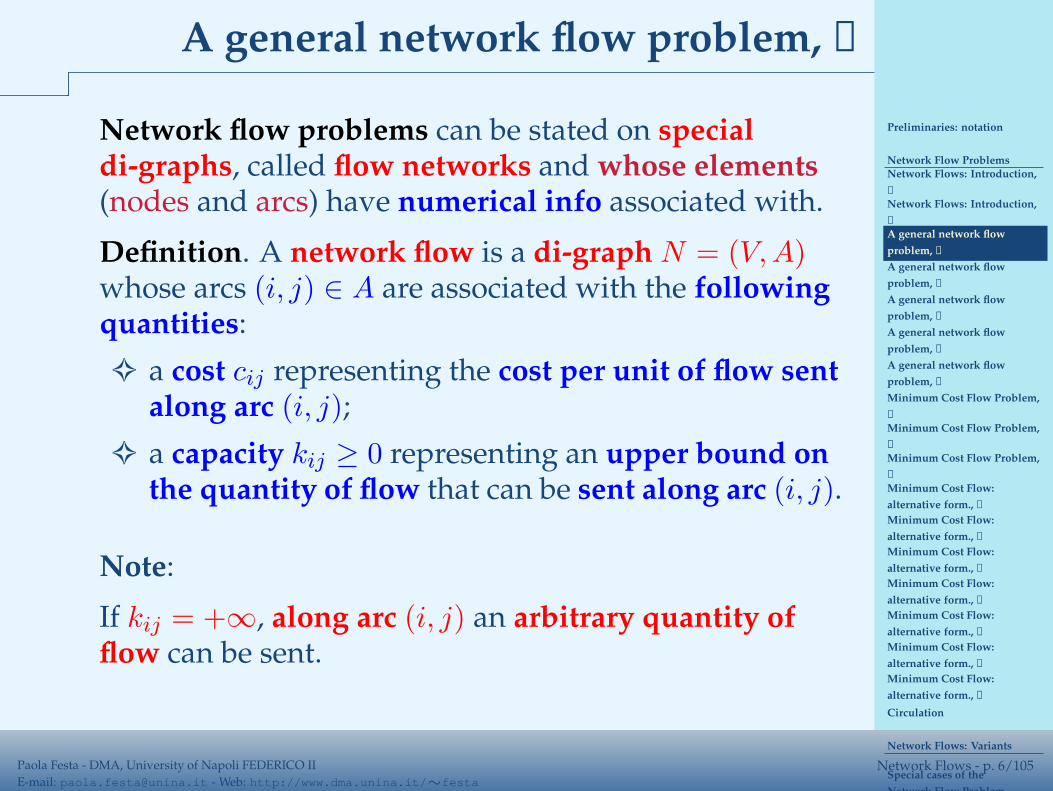
Network flow problems can be stated on specialdi-graphs, called flow networks and whose elements(nodes and arcs) have numerical info associated with.
Definition. A network flow is a di-graph N = (V,A)whose arcs (i, j) ∈ A are associated with the followingquantities:
✧ a cost cij representing the cost per unit of flow sentalong arc (i, j);
✧ a capacity kij ≥ 0 representing an upper bound onthe quantity of flow that can be sent along arc (i, j).
Preliminaries: notation
Network Flow ProblemsNetwork Flows: Introduction,
➀
Network Flows: Introduction,
➁
A general network flow
problem, ➀
A general network flow
problem, ➁
A general network flow
problem, ➂
A general network flow
problem, ➃
A general network flow
problem, ➃
Minimum Cost Flow Problem,
➀
Minimum Cost Flow Problem,
➁
Minimum Cost Flow Problem,
➁
Minimum Cost Flow:
alternative form., ➀
Minimum Cost Flow:
alternative form., ➁
Minimum Cost Flow:
alternative form., ➁
Minimum Cost Flow:
alternative form., ➁
Minimum Cost Flow:
alternative form., ➁
Minimum Cost Flow:
alternative form., ➁
Minimum Cost Flow:
alternative form., ➂
Circulation
Network Flows: Variants
Special cases of the
Network Flow Problem
Paola Festa - DMA, University of Napoli FEDERICO II
E-mail: [email protected] - Web: http://www.dma.unina.it/∼festaNetwork Flows - p. 6/105
A general network flow problem, ➀
Network flow problems can be stated on specialdi-graphs, called flow networks and whose elements(nodes and arcs) have numerical info associated with.
Definition. A network flow is a di-graph N = (V,A)whose arcs (i, j) ∈ A are associated with the followingquantities:
✧ a cost cij representing the cost per unit of flow sentalong arc (i, j);
✧ a capacity kij ≥ 0 representing an upper bound onthe quantity of flow that can be sent along arc (i, j).
Note:
If kij = +∞, along arc (i, j) an arbitrary quantity offlow can be sent.
Preliminaries: notation
Network Flow ProblemsNetwork Flows: Introduction,
➀
Network Flows: Introduction,
➁
A general network flow
problem, ➀
A general network flow
problem, ➁
A general network flow
problem, ➂
A general network flow
problem, ➃
A general network flow
problem, ➃
Minimum Cost Flow Problem,
➀
Minimum Cost Flow Problem,
➁
Minimum Cost Flow Problem,
➁
Minimum Cost Flow:
alternative form., ➀
Minimum Cost Flow:
alternative form., ➁
Minimum Cost Flow:
alternative form., ➁
Minimum Cost Flow:
alternative form., ➁
Minimum Cost Flow:
alternative form., ➁
Minimum Cost Flow:
alternative form., ➁
Minimum Cost Flow:
alternative form., ➂
Circulation
Network Flows: Variants
Special cases of the
Network Flow Problem
Paola Festa - DMA, University of Napoli FEDERICO II
E-mail: [email protected] - Web: http://www.dma.unina.it/∼festaNetwork Flows - p. 7/105
A general network flow problem, ➁
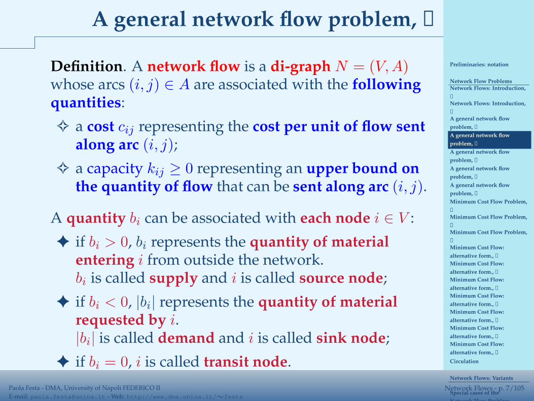
Definition. A network flow is a di-graph N = (V,A)whose arcs (i, j) ∈ A are associated with the followingquantities:
✧ a cost cij representing the cost per unit of flow sentalong arc (i, j);
✧ a capacity kij ≥ 0 representing an upper bound onthe quantity of flow that can be sent along arc (i, j).
A quantity bi can be associated with each node i ∈ V :
✦ if bi > 0, bi represents the quantity of materialentering i from outside the network.bi is called supply and i is called source node;
✦ if bi < 0, |bi| represents the quantity of materialrequested by i.|bi| is called demand and i is called sink node;
✦ if bi = 0, i is called transit node.

Preliminaries: notation
Network Flow ProblemsNetwork Flows: Introduction,
➀
Network Flows: Introduction,
➁
A general network flow
problem, ➀
A general network flow
problem, ➁
A general network flow
problem, ➂
A general network flow
problem, ➃
A general network flow
problem, ➃
Minimum Cost Flow Problem,
➀
Minimum Cost Flow Problem,
➁
Minimum Cost Flow Problem,
➁
Minimum Cost Flow:
alternative form., ➀
Minimum Cost Flow:
alternative form., ➁
Minimum Cost Flow:
alternative form., ➁
Minimum Cost Flow:
alternative form., ➁
Minimum Cost Flow:
alternative form., ➁
Minimum Cost Flow:
alternative form., ➁
Minimum Cost Flow:
alternative form., ➂
Circulation
Network Flows: Variants
Special cases of the
Network Flow Problem
Paola Festa - DMA, University of Napoli FEDERICO II
E-mail: [email protected] - Web: http://www.dma.unina.it/∼festaNetwork Flows - p. 8/105
A general network flow problem, ➂
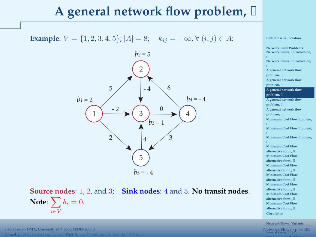
Example. V = {1, 2, 3, 4, 5}; |A| = 8; kij = +∞, ∀ (i, j) ∈ A:
10
b1 = 2
2
3 4
5
6
4 3
- 4
- 2
5
2
b2 = 5
b4 = - 4
b5 = - 4
b3 = 1

Preliminaries: notation
Network Flow ProblemsNetwork Flows: Introduction,
➀
Network Flows: Introduction,
➁
A general network flow
problem, ➀
A general network flow
problem, ➁
A general network flow
problem, ➂
A general network flow
problem, ➃
A general network flow
problem, ➃
Minimum Cost Flow Problem,
➀
Minimum Cost Flow Problem,
➁
Minimum Cost Flow Problem,
➁
Minimum Cost Flow:
alternative form., ➀
Minimum Cost Flow:
alternative form., ➁
Minimum Cost Flow:
alternative form., ➁
Minimum Cost Flow:
alternative form., ➁
Minimum Cost Flow:
alternative form., ➁
Minimum Cost Flow:
alternative form., ➁
Minimum Cost Flow:
alternative form., ➂
Circulation
Network Flows: Variants
Special cases of the
Network Flow Problem
Paola Festa - DMA, University of Napoli FEDERICO II
E-mail: [email protected] - Web: http://www.dma.unina.it/∼festaNetwork Flows - p. 8/105
A general network flow problem, ➂
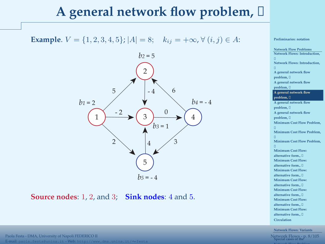
Example. V = {1, 2, 3, 4, 5}; |A| = 8; kij = +∞, ∀ (i, j) ∈ A:
10
b1 = 2
2
3 4
5
6
4 3
- 4
- 2
5
2
b2 = 5
b4 = - 4
b5 = - 4
b3 = 1
Source nodes: 1, 2, and 3;
Preliminaries: notation
Network Flow ProblemsNetwork Flows: Introduction,
➀
Network Flows: Introduction,
➁
A general network flow
problem, ➀
A general network flow
problem, ➁
A general network flow
problem, ➂
A general network flow
problem, ➃
A general network flow
problem, ➃
Minimum Cost Flow Problem,
➀
Minimum Cost Flow Problem,
➁
Minimum Cost Flow Problem,
➁
Minimum Cost Flow:
alternative form., ➀
Minimum Cost Flow:
alternative form., ➁
Minimum Cost Flow:
alternative form., ➁
Minimum Cost Flow:
alternative form., ➁
Minimum Cost Flow:
alternative form., ➁
Minimum Cost Flow:
alternative form., ➁
Minimum Cost Flow:
alternative form., ➂
Circulation
Network Flows: Variants
Special cases of the
Network Flow Problem
Paola Festa - DMA, University of Napoli FEDERICO II
E-mail: [email protected] - Web: http://www.dma.unina.it/∼festaNetwork Flows - p. 8/105
A general network flow problem, ➂
Example. V = {1, 2, 3, 4, 5}; |A| = 8; kij = +∞, ∀ (i, j) ∈ A:
10
b1 = 2
2
3 4
5
6
4 3
- 4
- 2
5
2
b2 = 5
b4 = - 4
b5 = - 4
b3 = 1
Source nodes: 1, 2, and 3; Sink nodes: 4 and 5.
Preliminaries: notation
Network Flow ProblemsNetwork Flows: Introduction,
➀
Network Flows: Introduction,
➁
A general network flow
problem, ➀
A general network flow
problem, ➁
A general network flow
problem, ➂
A general network flow
problem, ➃
A general network flow
problem, ➃
Minimum Cost Flow Problem,
➀
Minimum Cost Flow Problem,
➁
Minimum Cost Flow Problem,
➁
Minimum Cost Flow:
alternative form., ➀
Minimum Cost Flow:
alternative form., ➁
Minimum Cost Flow:
alternative form., ➁
Minimum Cost Flow:
alternative form., ➁
Minimum Cost Flow:
alternative form., ➁
Minimum Cost Flow:
alternative form., ➁
Minimum Cost Flow:
alternative form., ➂
Circulation
Network Flows: Variants
Special cases of the
Network Flow Problem
Paola Festa - DMA, University of Napoli FEDERICO II
E-mail: [email protected] - Web: http://www.dma.unina.it/∼festaNetwork Flows - p. 8/105
A general network flow problem, ➂
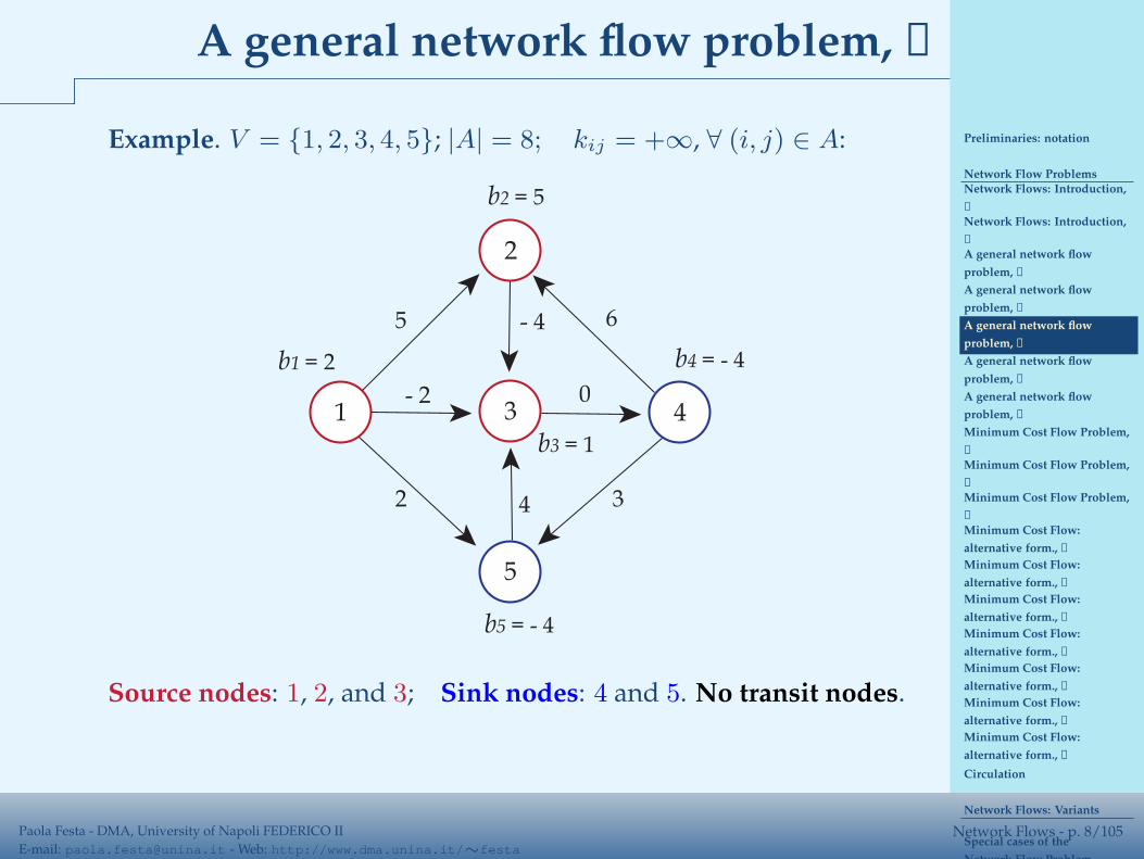
Example. V = {1, 2, 3, 4, 5}; |A| = 8; kij = +∞, ∀ (i, j) ∈ A:
10
b1 = 2
2
3 4
5
6
4 3
- 4
- 2
5
2
b2 = 5
b4 = - 4
b5 = - 4
b3 = 1
Source nodes: 1, 2, and 3; Sink nodes: 4 and 5. No transit nodes.
Preliminaries: notation
Network Flow ProblemsNetwork Flows: Introduction,
➀
Network Flows: Introduction,
➁
A general network flow
problem, ➀
A general network flow
problem, ➁
A general network flow
problem, ➂
A general network flow
problem, ➃
A general network flow
problem, ➃
Minimum Cost Flow Problem,
➀
Minimum Cost Flow Problem,
➁
Minimum Cost Flow Problem,
➁
Minimum Cost Flow:
alternative form., ➀
Minimum Cost Flow:
alternative form., ➁
Minimum Cost Flow:
alternative form., ➁
Minimum Cost Flow:
alternative form., ➁
Minimum Cost Flow:
alternative form., ➁
Minimum Cost Flow:
alternative form., ➁
Minimum Cost Flow:
alternative form., ➂
Circulation
Network Flows: Variants
Special cases of the
Network Flow Problem
Paola Festa - DMA, University of Napoli FEDERICO II
E-mail: [email protected] - Web: http://www.dma.unina.it/∼festaNetwork Flows - p. 8/105
A general network flow problem, ➂
Example. V = {1, 2, 3, 4, 5}; |A| = 8; kij = +∞, ∀ (i, j) ∈ A:
10
b1 = 2
2
3 4
5
6
4 3
- 4
- 2
5
2
b2 = 5
b4 = - 4
b5 = - 4
b3 = 1
Source nodes: 1, 2, and 3; Sink nodes: 4 and 5. No transit nodes.
Note:∑
i∈V
bi = 0.
Preliminaries: notation
Network Flow ProblemsNetwork Flows: Introduction,
➀
Network Flows: Introduction,
➁
A general network flow
problem, ➀
A general network flow
problem, ➁
A general network flow
problem, ➂
A general network flow
problem, ➃
A general network flow
problem, ➃
Minimum Cost Flow Problem,
➀
Minimum Cost Flow Problem,
➁
Minimum Cost Flow Problem,
➁
Minimum Cost Flow:
alternative form., ➀
Minimum Cost Flow:
alternative form., ➁
Minimum Cost Flow:
alternative form., ➁
Minimum Cost Flow:
alternative form., ➁
Minimum Cost Flow:
alternative form., ➁
Minimum Cost Flow:
alternative form., ➁
Minimum Cost Flow:
alternative form., ➂
Circulation
Network Flows: Variants
Special cases of the
Network Flow Problem
Paola Festa - DMA, University of Napoli FEDERICO II
E-mail: [email protected] - Web: http://www.dma.unina.it/∼festaNetwork Flows - p. 9/105
A general network flow problem, ➃
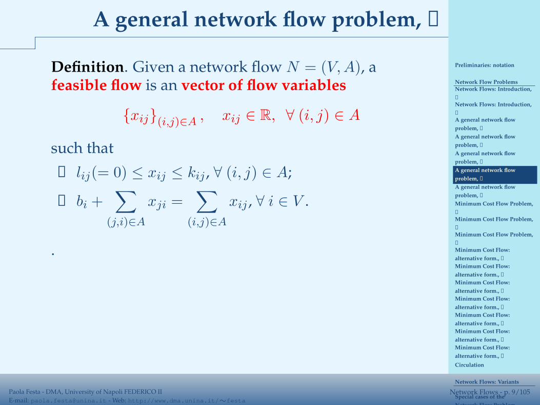
Definition. Given a network flow N = (V,A), afeasible flow is an vector of flow variables
{xij}(i,j)∈A , xij ∈ R, ∀ (i, j) ∈ A
such that
① lij(= 0) ≤ xij ≤ kij , ∀ (i, j) ∈ A;
② bi +∑
(j,i)∈A
xji =∑
(i,j)∈A
xij , ∀ i ∈ V .
.

Preliminaries: notation
Network Flow ProblemsNetwork Flows: Introduction,
➀
Network Flows: Introduction,
➁
A general network flow
problem, ➀
A general network flow
problem, ➁
A general network flow
problem, ➂
A general network flow
problem, ➃
A general network flow
problem, ➃
Minimum Cost Flow Problem,
➀
Minimum Cost Flow Problem,
➁
Minimum Cost Flow Problem,
➁
Minimum Cost Flow:
alternative form., ➀
Minimum Cost Flow:
alternative form., ➁
Minimum Cost Flow:
alternative form., ➁
Minimum Cost Flow:
alternative form., ➁
Minimum Cost Flow:
alternative form., ➁
Minimum Cost Flow:
alternative form., ➁
Minimum Cost Flow:
alternative form., ➂
Circulation
Network Flows: Variants
Special cases of the
Network Flow Problem
Paola Festa - DMA, University of Napoli FEDERICO II
E-mail: [email protected] - Web: http://www.dma.unina.it/∼festaNetwork Flows - p. 9/105
A general network flow problem, ➃
Definition. Given a network flow N = (V,A), afeasible flow is an vector of flow variables
{xij}(i,j)∈A , xij ∈ R, ∀ (i, j) ∈ A
such that
① lij(= 0) ≤ xij ≤ kij , ∀ (i, j) ∈ A;
② bi +∑
(j,i)∈A
xji =∑
(i,j)∈A
xij , ∀ i ∈ V .
Conditions ① are easy to understand.
Preliminaries: notation
Network Flow ProblemsNetwork Flows: Introduction,
➀
Network Flows: Introduction,
➁
A general network flow
problem, ➀
A general network flow
problem, ➁
A general network flow
problem, ➂
A general network flow
problem, ➃
A general network flow
problem, ➃
Minimum Cost Flow Problem,
➀
Minimum Cost Flow Problem,
➁
Minimum Cost Flow Problem,
➁
Minimum Cost Flow:
alternative form., ➀
Minimum Cost Flow:
alternative form., ➁
Minimum Cost Flow:
alternative form., ➁
Minimum Cost Flow:
alternative form., ➁
Minimum Cost Flow:
alternative form., ➁
Minimum Cost Flow:
alternative form., ➁
Minimum Cost Flow:
alternative form., ➂
Circulation
Network Flows: Variants
Special cases of the
Network Flow Problem
Paola Festa - DMA, University of Napoli FEDERICO II
E-mail: [email protected] - Web: http://www.dma.unina.it/∼festaNetwork Flows - p. 9/105
A general network flow problem, ➃
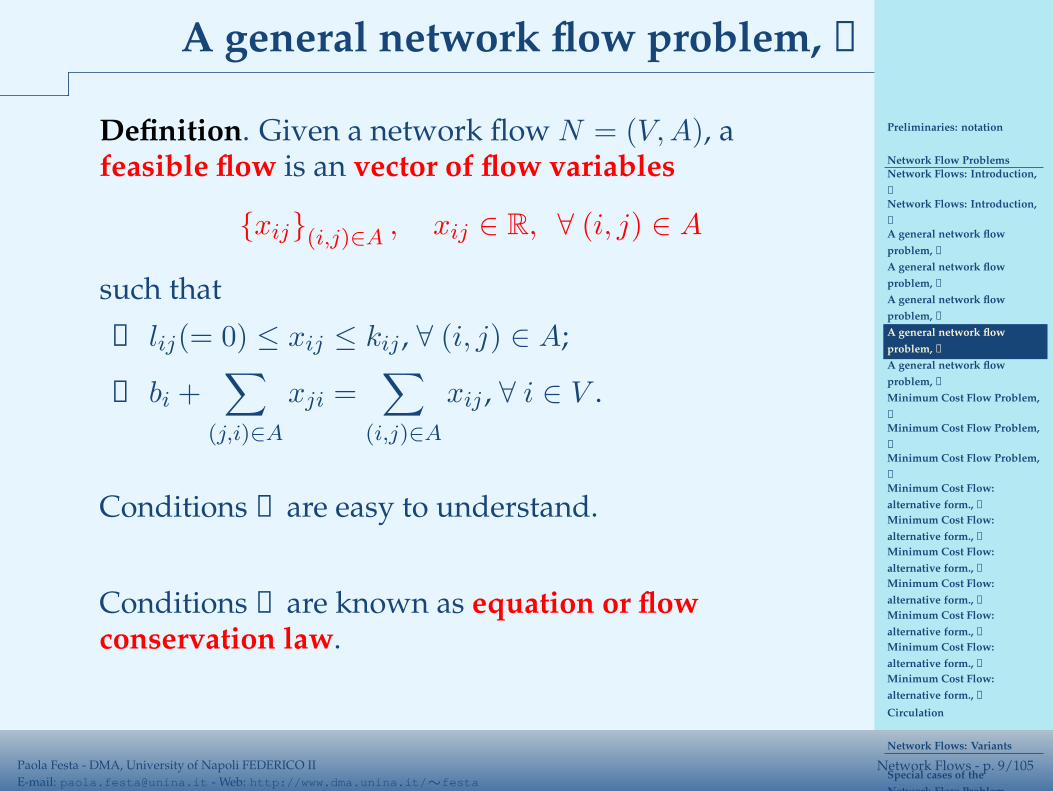
Definition. Given a network flow N = (V,A), afeasible flow is an vector of flow variables
{xij}(i,j)∈A , xij ∈ R, ∀ (i, j) ∈ A
such that
① lij(= 0) ≤ xij ≤ kij , ∀ (i, j) ∈ A;
② bi +∑
(j,i)∈A
xji =∑
(i,j)∈A
xij , ∀ i ∈ V .
Conditions ① are easy to understand.
Conditions ② are known as equation or flowconservation law.

Preliminaries: notation
Network Flow ProblemsNetwork Flows: Introduction,
➀
Network Flows: Introduction,
➁
A general network flow
problem, ➀
A general network flow
problem, ➁
A general network flow
problem, ➂
A general network flow
problem, ➃
A general network flow
problem, ➃
Minimum Cost Flow Problem,
➀
Minimum Cost Flow Problem,
➁
Minimum Cost Flow Problem,
➁
Minimum Cost Flow:
alternative form., ➀
Minimum Cost Flow:
alternative form., ➁
Minimum Cost Flow:
alternative form., ➁
Minimum Cost Flow:
alternative form., ➁
Minimum Cost Flow:
alternative form., ➁
Minimum Cost Flow:
alternative form., ➁
Minimum Cost Flow:
alternative form., ➂
Circulation
Network Flows: Variants
Special cases of the
Network Flow Problem
Paola Festa - DMA, University of Napoli FEDERICO II
E-mail: [email protected] - Web: http://www.dma.unina.it/∼festaNetwork Flows - p. 10/105
A general network flow problem, ➃
Definition. Given a network flow N = (V,A), afeasible flow is an vector of flow variables
{xij}(i,j)∈A , xij ∈ R, ∀ (i, j) ∈ A
such that
① lij(= 0) ≤ xij ≤ kij , ∀ (i, j) ∈ A;
② bi +∑
(j,i)∈A
xji =∑
(i,j)∈A
xij , ∀ i ∈ V .
Note: adding all over nodes i ∈ V both sides of ②, itresults that
∑
i∈V
bi = 0. (Principle of the total divergence)
The vector {bi}i∈V is called divergence vector.
Preliminaries: notation
Network Flow ProblemsNetwork Flows: Introduction,
➀
Network Flows: Introduction,
➁
A general network flow
problem, ➀
A general network flow
problem, ➁
A general network flow
problem, ➂
A general network flow
problem, ➃
A general network flow
problem, ➃
Minimum Cost Flow Problem,
➀
Minimum Cost Flow Problem,
➁
Minimum Cost Flow Problem,
➁
Minimum Cost Flow:
alternative form., ➀
Minimum Cost Flow:
alternative form., ➁
Minimum Cost Flow:
alternative form., ➁
Minimum Cost Flow:
alternative form., ➁
Minimum Cost Flow:
alternative form., ➁
Minimum Cost Flow:
alternative form., ➁
Minimum Cost Flow:
alternative form., ➂
Circulation
Network Flows: Variants
Special cases of the
Network Flow Problem
Paola Festa - DMA, University of Napoli FEDERICO II
E-mail: [email protected] - Web: http://www.dma.unina.it/∼festaNetwork Flows - p. 11/105
Minimum Cost Flow Problem, ➀
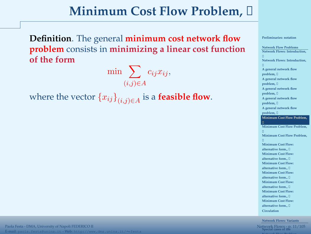
Definition. The general minimum cost network flowproblem consists in minimizing a linear cost functionof the form
min∑
(i,j)∈A
cijxij ,
where the vector {xij}(i,j)∈A is a feasible flow.

Preliminaries: notation
Network Flow ProblemsNetwork Flows: Introduction,
➀
Network Flows: Introduction,
➁
A general network flow
problem, ➀
A general network flow
problem, ➁
A general network flow
problem, ➂
A general network flow
problem, ➃
A general network flow
problem, ➃
Minimum Cost Flow Problem,
➀
Minimum Cost Flow Problem,
➁
Minimum Cost Flow Problem,
➁
Minimum Cost Flow:
alternative form., ➀
Minimum Cost Flow:
alternative form., ➁
Minimum Cost Flow:
alternative form., ➁
Minimum Cost Flow:
alternative form., ➁
Minimum Cost Flow:
alternative form., ➁
Minimum Cost Flow:
alternative form., ➁
Minimum Cost Flow:
alternative form., ➂
Circulation
Network Flows: Variants
Special cases of the
Network Flow Problem
Paola Festa - DMA, University of Napoli FEDERICO II
E-mail: [email protected] - Web: http://www.dma.unina.it/∼festaNetwork Flows - p. 11/105
Minimum Cost Flow Problem, ➀
Definition. The general minimum cost network flowproblem consists in minimizing a linear cost functionof the form
min∑
(i,j)∈A
cijxij ,
where the vector {xij}(i,j)∈A is a feasible flow.
(MF) min∑
(i,j)∈A
cijxij
s.t.
(a)∑
(i,j)∈A
xij −
bi +∑
(j,i)∈A
xji
= 0, ∀ i ∈ V
(b) lij ≤ xij ≤ kij , ∀(i, j) ∈ A.
Preliminaries: notation
Network Flow ProblemsNetwork Flows: Introduction,
➀
Network Flows: Introduction,
➁
A general network flow
problem, ➀
A general network flow
problem, ➁
A general network flow
problem, ➂
A general network flow
problem, ➃
A general network flow
problem, ➃
Minimum Cost Flow Problem,
➀
Minimum Cost Flow Problem,
➁
Minimum Cost Flow Problem,
➁
Minimum Cost Flow:
alternative form., ➀
Minimum Cost Flow:
alternative form., ➁
Minimum Cost Flow:
alternative form., ➁
Minimum Cost Flow:
alternative form., ➁
Minimum Cost Flow:
alternative form., ➁
Minimum Cost Flow:
alternative form., ➁
Minimum Cost Flow:
alternative form., ➂
Circulation
Network Flows: Variants
Special cases of the
Network Flow Problem
Paola Festa - DMA, University of Napoli FEDERICO II
E-mail: [email protected] - Web: http://www.dma.unina.it/∼festaNetwork Flows - p. 12/105
Minimum Cost Flow Problem, ➁
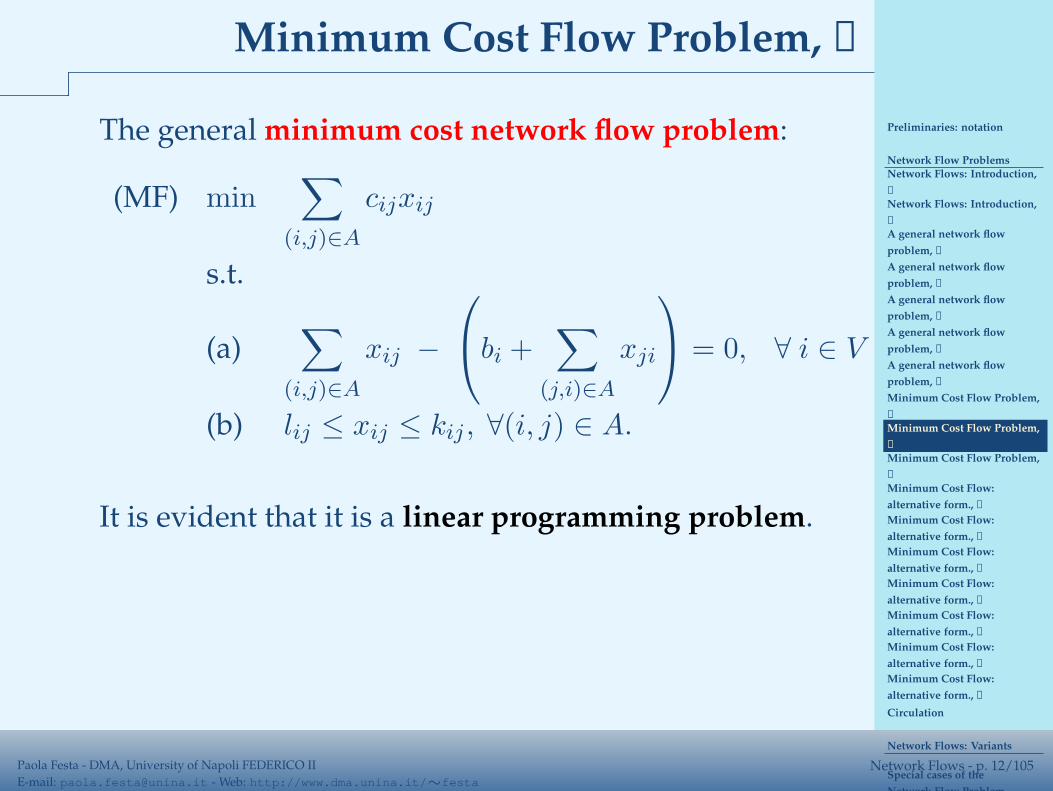
The general minimum cost network flow problem:
(MF) min∑
(i,j)∈A
cijxij
s.t.
(a)∑
(i,j)∈A
xij −
bi +∑
(j,i)∈A
xji
= 0, ∀ i ∈ V
(b) lij ≤ xij ≤ kij , ∀(i, j) ∈ A.
It is evident that it is a linear programming problem.
Preliminaries: notation
Network Flow ProblemsNetwork Flows: Introduction,
➀
Network Flows: Introduction,
➁
A general network flow
problem, ➀
A general network flow
problem, ➁
A general network flow
problem, ➂
A general network flow
problem, ➃
A general network flow
problem, ➃
Minimum Cost Flow Problem,
➀
Minimum Cost Flow Problem,
➁
Minimum Cost Flow Problem,
➁
Minimum Cost Flow:
alternative form., ➀
Minimum Cost Flow:
alternative form., ➁
Minimum Cost Flow:
alternative form., ➁
Minimum Cost Flow:
alternative form., ➁
Minimum Cost Flow:
alternative form., ➁
Minimum Cost Flow:
alternative form., ➁
Minimum Cost Flow:
alternative form., ➂
Circulation
Network Flows: Variants
Special cases of the
Network Flow Problem
Paola Festa - DMA, University of Napoli FEDERICO II
E-mail: [email protected] - Web: http://www.dma.unina.it/∼festaNetwork Flows - p. 12/105
Minimum Cost Flow Problem, ➁
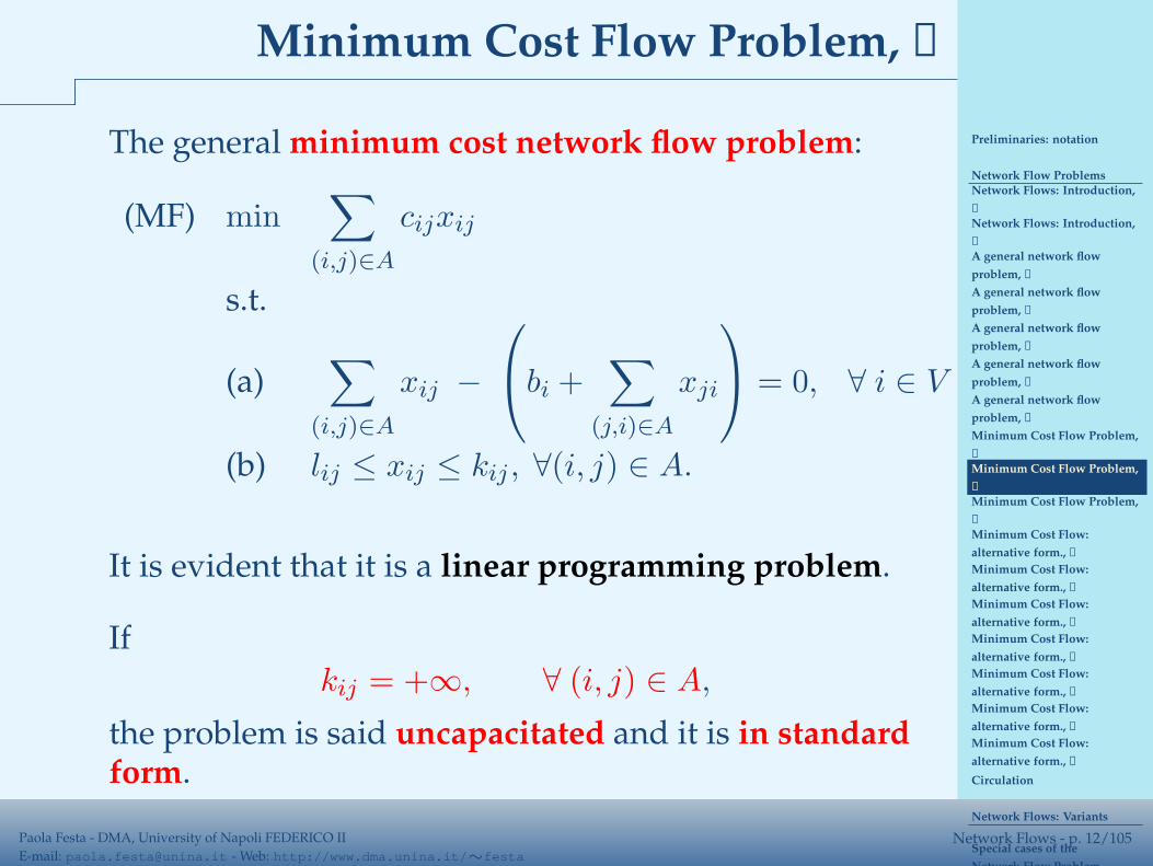
The general minimum cost network flow problem:
(MF) min∑
(i,j)∈A
cijxij
s.t.
(a)∑
(i,j)∈A
xij −
bi +∑
(j,i)∈A
xji
= 0, ∀ i ∈ V
(b) lij ≤ xij ≤ kij , ∀(i, j) ∈ A.
It is evident that it is a linear programming problem.
If
kij = +∞, ∀ (i, j) ∈ A,
the problem is said uncapacitated and it is in standardform.
Preliminaries: notation
Network Flow ProblemsNetwork Flows: Introduction,
➀
Network Flows: Introduction,
➁
A general network flow
problem, ➀
A general network flow
problem, ➁
A general network flow
problem, ➂
A general network flow
problem, ➃
A general network flow
problem, ➃
Minimum Cost Flow Problem,
➀
Minimum Cost Flow Problem,
➁
Minimum Cost Flow Problem,
➁
Minimum Cost Flow:
alternative form., ➀
Minimum Cost Flow:
alternative form., ➁
Minimum Cost Flow:
alternative form., ➁
Minimum Cost Flow:
alternative form., ➁
Minimum Cost Flow:
alternative form., ➁
Minimum Cost Flow:
alternative form., ➁
Minimum Cost Flow:
alternative form., ➂
Circulation
Network Flows: Variants
Special cases of the
Network Flow Problem
Paola Festa - DMA, University of Napoli FEDERICO II
E-mail: [email protected] - Web: http://www.dma.unina.it/∼festaNetwork Flows - p. 13/105
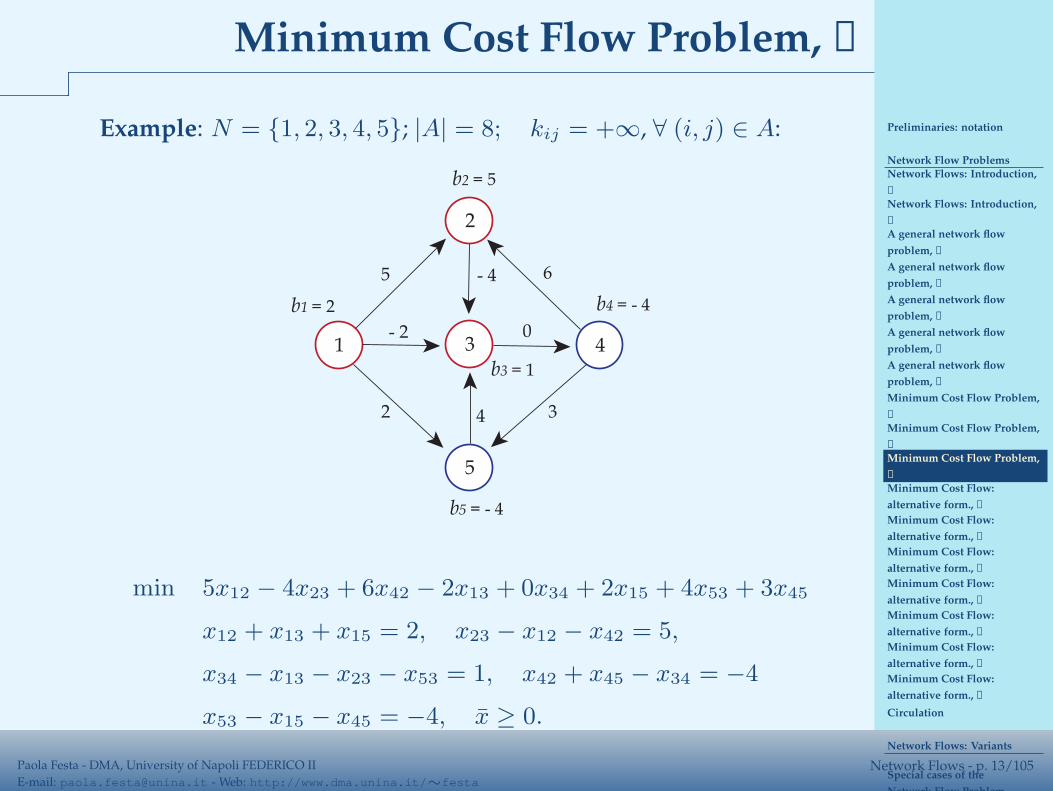
Minimum Cost Flow Problem, ➁
Example: N = {1, 2, 3, 4, 5}; |A| = 8; kij = +∞, ∀ (i, j) ∈ A:
10
b1 = 2
2
3 4
5
6
4 3
- 4
- 2
5
2
b2 = 5
b4 = - 4
b5 = - 4
b3 = 1
min 5x12 − 4x23 + 6x42 − 2x13 + 0x34 + 2x15 + 4x53 + 3x45
x12 + x13 + x15 = 2, x23 − x12 − x42 = 5,
x34 − x13 − x23 − x53 = 1, x42 + x45 − x34 = −4
x53 − x15 − x45 = −4, x̄ ≥ 0.
Preliminaries: notation
Network Flow ProblemsNetwork Flows: Introduction,
➀
Network Flows: Introduction,
➁
A general network flow
problem, ➀
A general network flow
problem, ➁
A general network flow
problem, ➂
A general network flow
problem, ➃
A general network flow
problem, ➃
Minimum Cost Flow Problem,
➀
Minimum Cost Flow Problem,
➁
Minimum Cost Flow Problem,
➁
Minimum Cost Flow:
alternative form., ➀
Minimum Cost Flow:
alternative form., ➁
Minimum Cost Flow:
alternative form., ➁
Minimum Cost Flow:
alternative form., ➁
Minimum Cost Flow:
alternative form., ➁
Minimum Cost Flow:
alternative form., ➁
Minimum Cost Flow:
alternative form., ➂
Circulation
Network Flows: Variants
Special cases of the
Network Flow Problem
Paola Festa - DMA, University of Napoli FEDERICO II
E-mail: [email protected] - Web: http://www.dma.unina.it/∼festaNetwork Flows - p. 14/105
Minimum Cost Flow: alternative form., ➀
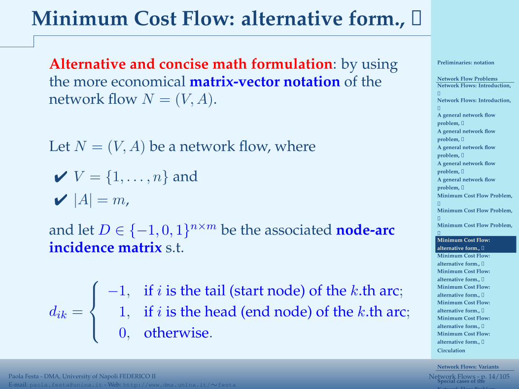
Alternative and concise math formulation: by usingthe more economical matrix-vector notation of thenetwork flow N = (V,A).
Preliminaries: notation
Network Flow ProblemsNetwork Flows: Introduction,
➀
Network Flows: Introduction,
➁
A general network flow
problem, ➀
A general network flow
problem, ➁
A general network flow
problem, ➂
A general network flow
problem, ➃
A general network flow
problem, ➃
Minimum Cost Flow Problem,
➀
Minimum Cost Flow Problem,
➁
Minimum Cost Flow Problem,
➁
Minimum Cost Flow:
alternative form., ➀
Minimum Cost Flow:
alternative form., ➁
Minimum Cost Flow:
alternative form., ➁
Minimum Cost Flow:
alternative form., ➁
Minimum Cost Flow:
alternative form., ➁
Minimum Cost Flow:
alternative form., ➁
Minimum Cost Flow:
alternative form., ➂
Circulation
Network Flows: Variants
Special cases of the
Network Flow Problem
Paola Festa - DMA, University of Napoli FEDERICO II
E-mail: [email protected] - Web: http://www.dma.unina.it/∼festaNetwork Flows - p. 14/105
Minimum Cost Flow: alternative form., ➀
Alternative and concise math formulation: by usingthe more economical matrix-vector notation of thenetwork flow N = (V,A).
Let N = (V,A) be a network flow, where
✔ V = {1, . . . , n} and
✔ |A| = m,
and let D ∈ {−1, 0, 1}n×m be the associated node-arcincidence matrix s.t.
dik =
−1, if i is the tail (start node) of the k.th arc;
1, if i is the head (end node) of the k.th arc;
0, otherwise.
Preliminaries: notation
Network Flow ProblemsNetwork Flows: Introduction,
➀
Network Flows: Introduction,
➁
A general network flow
problem, ➀
A general network flow
problem, ➁
A general network flow
problem, ➂
A general network flow
problem, ➃
A general network flow
problem, ➃
Minimum Cost Flow Problem,
➀
Minimum Cost Flow Problem,
➁
Minimum Cost Flow Problem,
➁
Minimum Cost Flow:
alternative form., ➀
Minimum Cost Flow:
alternative form., ➁
Minimum Cost Flow:
alternative form., ➁
Minimum Cost Flow:
alternative form., ➁
Minimum Cost Flow:
alternative form., ➁
Minimum Cost Flow:
alternative form., ➁
Minimum Cost Flow:
alternative form., ➂
Circulation
Network Flows: Variants
Special cases of the
Network Flow Problem
Paola Festa - DMA, University of Napoli FEDERICO II
E-mail: [email protected] - Web: http://www.dma.unina.it/∼festaNetwork Flows - p. 15/105
Minimum Cost Flow: alternative form., ➁
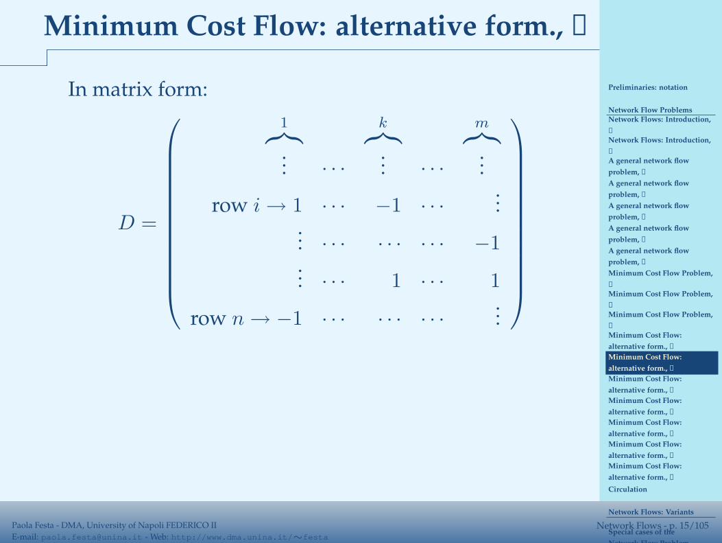
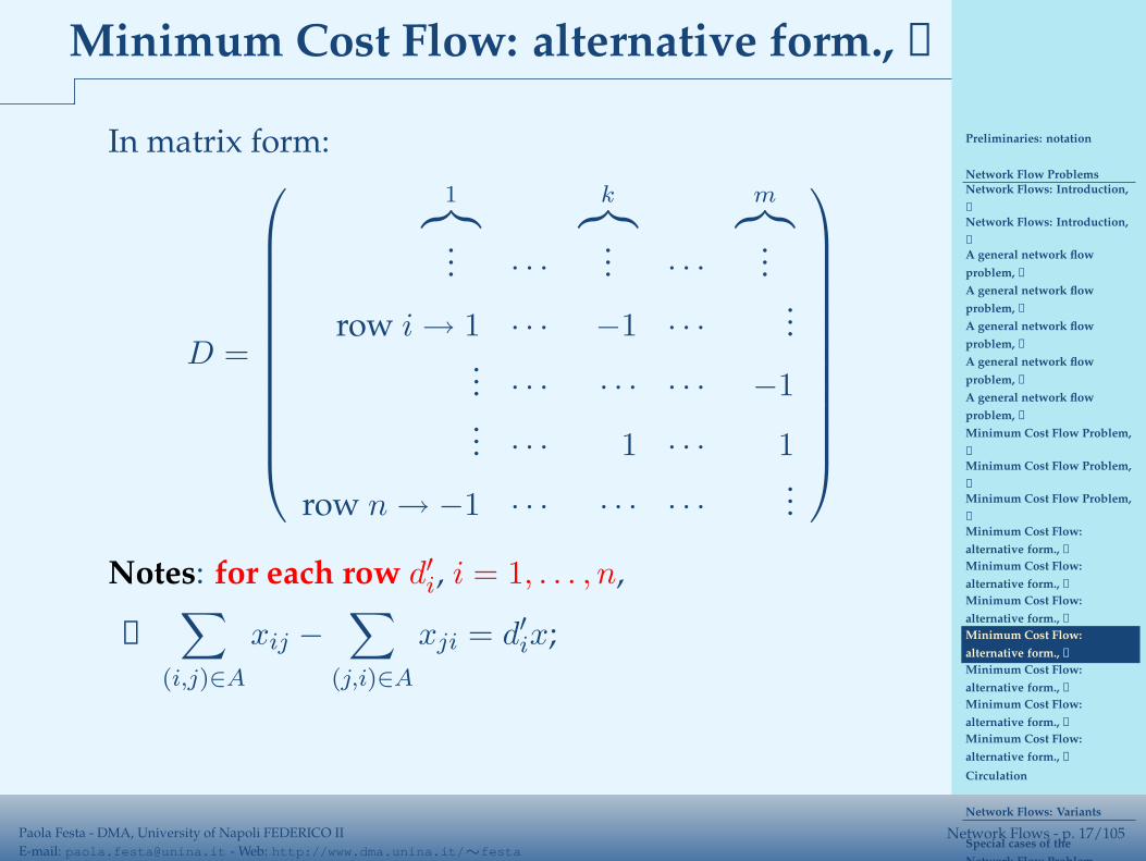
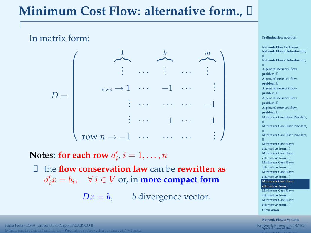
In matrix form:
D =
1︷︸︸︷
... · · ·
k︷︸︸︷
... · · ·
m︷︸︸︷
...
row i → 1 · · · −1 · · ·...
... · · · · · · · · · −1
... · · · 1 · · · 1
row n → −1 · · · · · · · · ·...
Preliminaries: notation
Network Flow ProblemsNetwork Flows: Introduction,
➀
Network Flows: Introduction,
➁
A general network flow
problem, ➀
A general network flow
problem, ➁
A general network flow
problem, ➂
A general network flow
problem, ➃
A general network flow
problem, ➃
Minimum Cost Flow Problem,
➀
Minimum Cost Flow Problem,
➁
Minimum Cost Flow Problem,
➁
Minimum Cost Flow:
alternative form., ➀
Minimum Cost Flow:
alternative form., ➁
Minimum Cost Flow:
alternative form., ➁
Minimum Cost Flow:
alternative form., ➁
Minimum Cost Flow:
alternative form., ➁
Minimum Cost Flow:
alternative form., ➁
Minimum Cost Flow:
alternative form., ➂
Circulation
Network Flows: Variants
Special cases of the
Network Flow Problem
Paola Festa - DMA, University of Napoli FEDERICO II
E-mail: [email protected] - Web: http://www.dma.unina.it/∼festaNetwork Flows - p. 15/105
Minimum Cost Flow: alternative form., ➁
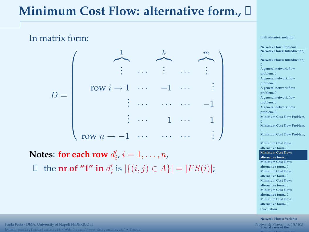
In matrix form:
D =
1︷︸︸︷
... · · ·
k︷︸︸︷
... · · ·
m︷︸︸︷
...
row i → 1 · · · −1 · · ·...
... · · · · · · · · · −1
... · · · 1 · · · 1
row n → −1 · · · · · · · · ·...
Notes: for each row d′i, i = 1, . . . , n,
① the nr of “1” in d′i is |{(i, j) ∈ A}| = |FS(i)|;
Preliminaries: notation
Network Flow ProblemsNetwork Flows: Introduction,
➀
Network Flows: Introduction,
➁
A general network flow
problem, ➀
A general network flow
problem, ➁
A general network flow
problem, ➂
A general network flow
problem, ➃
A general network flow
problem, ➃
Minimum Cost Flow Problem,
➀
Minimum Cost Flow Problem,
➁
Minimum Cost Flow Problem,
➁
Minimum Cost Flow:
alternative form., ➀
Minimum Cost Flow:
alternative form., ➁
Minimum Cost Flow:
alternative form., ➁
Minimum Cost Flow:
alternative form., ➁
Minimum Cost Flow:
alternative form., ➁
Minimum Cost Flow:
alternative form., ➁
Minimum Cost Flow:
alternative form., ➂
Circulation
Network Flows: Variants
Special cases of the
Network Flow Problem
Paola Festa - DMA, University of Napoli FEDERICO II
E-mail: [email protected] - Web: http://www.dma.unina.it/∼festaNetwork Flows - p. 16/105
Minimum Cost Flow: alternative form., ➁
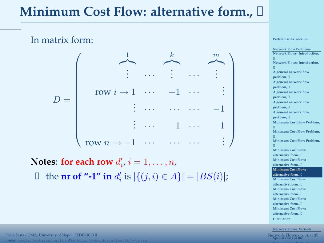
In matrix form:
D =
1︷︸︸︷
... · · ·
k︷︸︸︷
... · · ·
m︷︸︸︷
...
row i → 1 · · · −1 · · ·...
... · · · · · · · · · −1
... · · · 1 · · · 1
row n → −1 · · · · · · · · ·...
Notes: for each row d′i, i = 1, . . . , n,
② the nr of “-1” in d′i is |{(j, i) ∈ A}| = |BS(i)|;
Preliminaries: notation
Network Flow ProblemsNetwork Flows: Introduction,
➀
Network Flows: Introduction,
➁
A general network flow
problem, ➀
A general network flow
problem, ➁
A general network flow
problem, ➂
A general network flow
problem, ➃
A general network flow
problem, ➃
Minimum Cost Flow Problem,
➀
Minimum Cost Flow Problem,
➁
Minimum Cost Flow Problem,
➁
Minimum Cost Flow:
alternative form., ➀
Minimum Cost Flow:
alternative form., ➁
Minimum Cost Flow:
alternative form., ➁
Minimum Cost Flow:
alternative form., ➁
Minimum Cost Flow:
alternative form., ➁
Minimum Cost Flow:
alternative form., ➁
Minimum Cost Flow:
alternative form., ➂
Circulation
Network Flows: Variants
Special cases of the
Network Flow Problem
Paola Festa - DMA, University of Napoli FEDERICO II
E-mail: [email protected] - Web: http://www.dma.unina.it/∼festaNetwork Flows - p. 17/105
Minimum Cost Flow: alternative form., ➁
In matrix form:
D =
1︷︸︸︷
... · · ·
k︷︸︸︷
... · · ·
m︷︸︸︷
...
row i → 1 · · · −1 · · ·...
... · · · · · · · · · −1
... · · · 1 · · · 1
row n → −1 · · · · · · · · ·...
Notes: for each row d′i, i = 1, . . . , n,
③∑
(i,j)∈A
xij −∑
(j,i)∈A
xji = d′ix;
Preliminaries: notation
Network Flow ProblemsNetwork Flows: Introduction,
➀
Network Flows: Introduction,
➁
A general network flow
problem, ➀
A general network flow
problem, ➁
A general network flow
problem, ➂
A general network flow
problem, ➃
A general network flow
problem, ➃
Minimum Cost Flow Problem,
➀
Minimum Cost Flow Problem,
➁
Minimum Cost Flow Problem,
➁
Minimum Cost Flow:
alternative form., ➀
Minimum Cost Flow:
alternative form., ➁
Minimum Cost Flow:
alternative form., ➁
Minimum Cost Flow:
alternative form., ➁
Minimum Cost Flow:
alternative form., ➁
Minimum Cost Flow:
alternative form., ➁
Minimum Cost Flow:
alternative form., ➂
Circulation
Network Flows: Variants
Special cases of the
Network Flow Problem
Paola Festa - DMA, University of Napoli FEDERICO II
E-mail: [email protected] - Web: http://www.dma.unina.it/∼festaNetwork Flows - p. 18/105
Minimum Cost Flow: alternative form., ➁
In matrix form:
D =
1︷︸︸︷
... · · ·
k︷︸︸︷
... · · ·
m︷︸︸︷
...
row i → 1 · · · −1 · · ·...
... · · · · · · · · · −1
... · · · 1 · · · 1
row n → −1 · · · · · · · · ·...
Notes: for each row d′i, i = 1, . . . , n
④ the flow conservation law can be rewritten asd′ix = bi, ∀ i ∈ V or, in more compact form
Dx = b, b divergence vector.

Preliminaries: notation
Network Flow ProblemsNetwork Flows: Introduction,
➀
Network Flows: Introduction,
➁
A general network flow
problem, ➀
A general network flow
problem, ➁
A general network flow
problem, ➂
A general network flow
problem, ➃
A general network flow
problem, ➃
Minimum Cost Flow Problem,
➀
Minimum Cost Flow Problem,
➁
Minimum Cost Flow Problem,
➁
Minimum Cost Flow:
alternative form., ➀
Minimum Cost Flow:
alternative form., ➁
Minimum Cost Flow:
alternative form., ➁
Minimum Cost Flow:
alternative form., ➁
Minimum Cost Flow:
alternative form., ➁
Minimum Cost Flow:
alternative form., ➁
Minimum Cost Flow:
alternative form., ➂
Circulation
Network Flows: Variants
Special cases of the
Network Flow Problem
Paola Festa - DMA, University of Napoli FEDERICO II
E-mail: [email protected] - Web: http://www.dma.unina.it/∼festaNetwork Flows - p. 19/105
Minimum Cost Flow: alternative form., ➁
In matrix form:
D =
1︷︸︸︷
... · · ·
k︷︸︸︷
... · · ·
m︷︸︸︷
...
row i → 1 · · · −1 · · ·...
... · · · · · · · · · −1
... · · · 1 · · · 1
row n → −1 · · · · · · · · ·...
Notes: for each row d′i, i = 1, . . . , n
⑤ adding all rows d′i results 0̄, i.e., the rows of D arel.d.Nevertheless, it is always possible to remove thereduntant constraints without changing thefeasible region of the problem.
Preliminaries: notation
Network Flow ProblemsNetwork Flows: Introduction,
➀
Network Flows: Introduction,
➁
A general network flow
problem, ➀
A general network flow
problem, ➁
A general network flow
problem, ➂
A general network flow
problem, ➃
A general network flow
problem, ➃
Minimum Cost Flow Problem,
➀
Minimum Cost Flow Problem,
➁
Minimum Cost Flow Problem,
➁
Minimum Cost Flow:
alternative form., ➀
Minimum Cost Flow:
alternative form., ➁
Minimum Cost Flow:
alternative form., ➁
Minimum Cost Flow:
alternative form., ➁
Minimum Cost Flow:
alternative form., ➁
Minimum Cost Flow:
alternative form., ➁
Minimum Cost Flow:
alternative form., ➂
Circulation
Network Flows: Variants
Special cases of the
Network Flow Problem
Paola Festa - DMA, University of Napoli FEDERICO II
E-mail: [email protected] - Web: http://www.dma.unina.it/∼festaNetwork Flows - p. 20/105
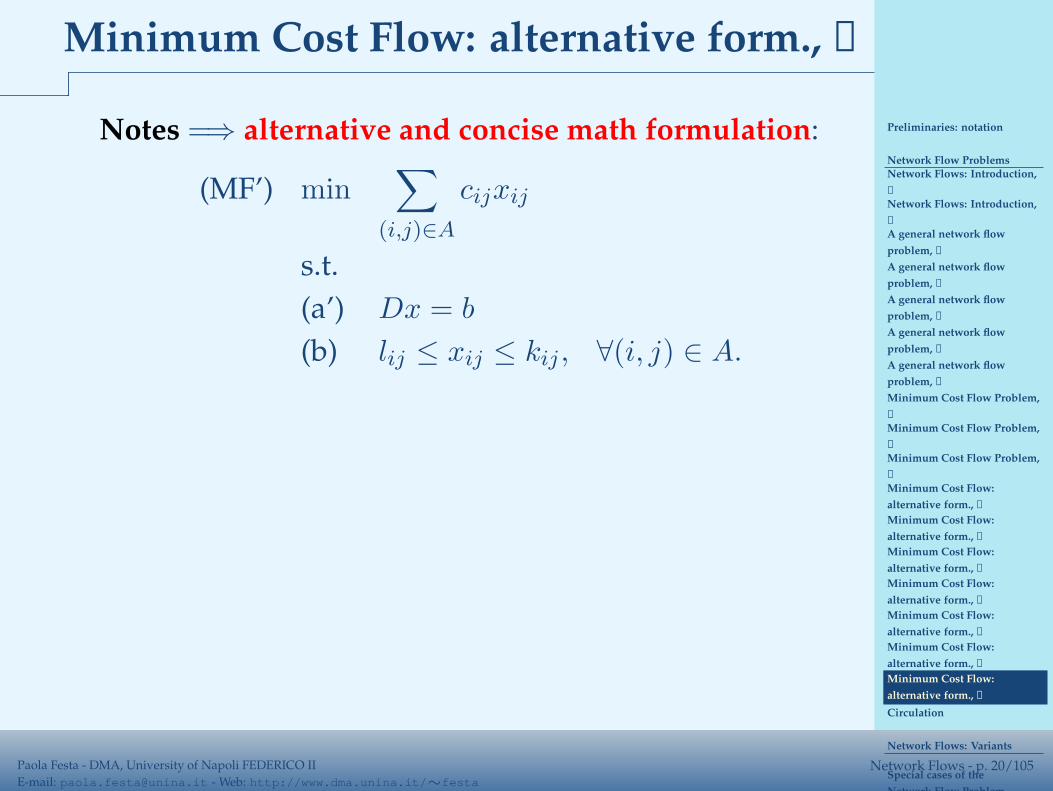
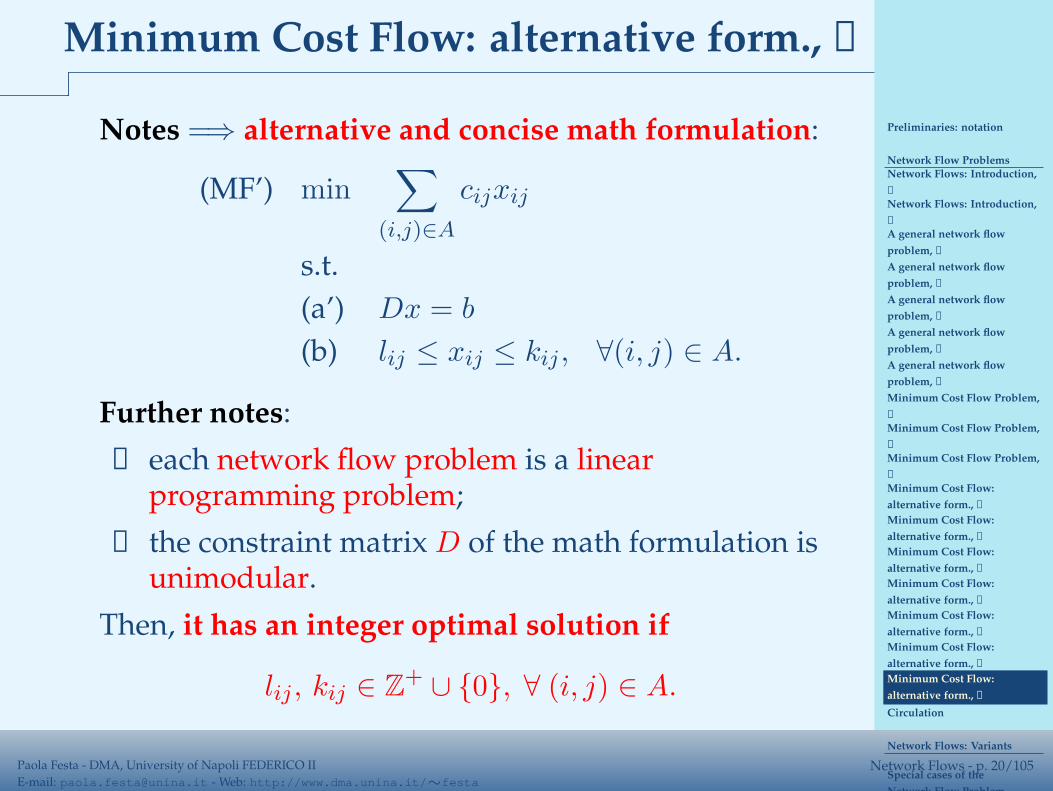
Minimum Cost Flow: alternative form., ➂
Notes =⇒ alternative and concise math formulation:
(MF’) min∑
(i,j)∈A
cijxij
s.t.
(a’) Dx = b
(b) lij ≤ xij ≤ kij , ∀(i, j) ∈ A.
Preliminaries: notation
Network Flow ProblemsNetwork Flows: Introduction,
➀
Network Flows: Introduction,
➁
A general network flow
problem, ➀
A general network flow
problem, ➁
A general network flow
problem, ➂
A general network flow
problem, ➃
A general network flow
problem, ➃
Minimum Cost Flow Problem,
➀
Minimum Cost Flow Problem,
➁
Minimum Cost Flow Problem,
➁
Minimum Cost Flow:
alternative form., ➀
Minimum Cost Flow:
alternative form., ➁
Minimum Cost Flow:
alternative form., ➁
Minimum Cost Flow:
alternative form., ➁
Minimum Cost Flow:
alternative form., ➁
Minimum Cost Flow:
alternative form., ➁
Minimum Cost Flow:
alternative form., ➂
Circulation
Network Flows: Variants
Special cases of the
Network Flow Problem
Paola Festa - DMA, University of Napoli FEDERICO II
E-mail: [email protected] - Web: http://www.dma.unina.it/∼festaNetwork Flows - p. 20/105
Minimum Cost Flow: alternative form., ➂
Notes =⇒ alternative and concise math formulation:
(MF’) min∑
(i,j)∈A
cijxij
s.t.
(a’) Dx = b
(b) lij ≤ xij ≤ kij , ∀(i, j) ∈ A.
Further notes:
❶ each network flow problem is a linearprogramming problem;
❷ the constraint matrix D of the math formulation isunimodular.
Then, it has an integer optimal solution if
lij , kij ∈ Z+ ∪ {0}, ∀ (i, j) ∈ A.
Preliminaries: notation
Network Flow ProblemsNetwork Flows: Introduction,
➀
Network Flows: Introduction,
➁
A general network flow
problem, ➀
A general network flow
problem, ➁
A general network flow
problem, ➂
A general network flow
problem, ➃
A general network flow
problem, ➃
Minimum Cost Flow Problem,
➀
Minimum Cost Flow Problem,
➁
Minimum Cost Flow Problem,
➁
Minimum Cost Flow:
alternative form., ➀
Minimum Cost Flow:
alternative form., ➁
Minimum Cost Flow:
alternative form., ➁
Minimum Cost Flow:
alternative form., ➁
Minimum Cost Flow:
alternative form., ➁
Minimum Cost Flow:
alternative form., ➁
Minimum Cost Flow:
alternative form., ➂
Circulation
Network Flows: Variants
Special cases of the
Network Flow Problem
Paola Festa - DMA, University of Napoli FEDERICO II
E-mail: [email protected] - Web: http://www.dma.unina.it/∼festaNetwork Flows - p. 21/105
Circulation
Definition. Any flow vector (feasible or infeasible) thatsatisfies
Dx = 0
is called circulation (in this case, it results that b = 0).
The flow conservation law (also known as Kirchkoff’sequation) is imposed only within the network,without external supply or demand.
In other words, the flow “circulates” only inside thenetwork.

Preliminaries: notation
Network Flow Problems
Network Flows: Variants
Network Flows: Variants
Network Flows: Variants
Network Flows: Variants
Network Flows: Variants
Network Flows: Variants
Network Flows: Variants
Special cases of the
Network Flow Problem
The Maximum Flow Problem
A solution method:
the Ford-Fulkerson algorithm
A simpler (not more efficient)
implementation
of Ford-Fulkerson algorithm
Ford-Fulkerson algorithm:
an exercise
Paola Festa - DMA, University of Napoli FEDERICO II
E-mail: [email protected] - Web: http://www.dma.unina.it/∼festaNetwork Flows - p. 22/105
Network Flows: Variants

Preliminaries: notation
Network Flow Problems
Network Flows: Variants
Network Flows: Variants
Network Flows: Variants
Network Flows: Variants
Network Flows: Variants
Network Flows: Variants
Network Flows: Variants
Special cases of the
Network Flow Problem
The Maximum Flow Problem
A solution method:
the Ford-Fulkerson algorithm
A simpler (not more efficient)
implementation
of Ford-Fulkerson algorithm
Ford-Fulkerson algorithm:
an exercise
Paola Festa - DMA, University of Napoli FEDERICO II
E-mail: [email protected] - Web: http://www.dma.unina.it/∼festaNetwork Flows - p. 23/105
Network Flows: Variants
There are several variants of network flow problems,all of which can be shown to be equivalent to eachother.
We will discuss now some examples.
Preliminaries: notation
Network Flow Problems
Network Flows: Variants
Network Flows: Variants
Network Flows: Variants
Network Flows: Variants
Network Flows: Variants
Network Flows: Variants
Network Flows: Variants
Special cases of the
Network Flow Problem
The Maximum Flow Problem
A solution method:
the Ford-Fulkerson algorithm
A simpler (not more efficient)
implementation
of Ford-Fulkerson algorithm
Ford-Fulkerson algorithm:
an exercise
Paola Festa - DMA, University of Napoli FEDERICO II
E-mail: [email protected] - Web: http://www.dma.unina.it/∼festaNetwork Flows - p. 24/105
Network Flows: Variants
Variant ①:Every network flow problem can be reduced to onewith exactly one source s and exactly one sink node d,s, d ∈ V , s 6= d.
Preliminaries: notation
Network Flow Problems
Network Flows: Variants
Network Flows: Variants
Network Flows: Variants
Network Flows: Variants
Network Flows: Variants
Network Flows: Variants
Network Flows: Variants
Special cases of the
Network Flow Problem
The Maximum Flow Problem
A solution method:
the Ford-Fulkerson algorithm
A simpler (not more efficient)
implementation
of Ford-Fulkerson algorithm
Ford-Fulkerson algorithm:
an exercise
Paola Festa - DMA, University of Napoli FEDERICO II
E-mail: [email protected] - Web: http://www.dma.unina.it/∼festaNetwork Flows - p. 24/105
Network Flows: Variants
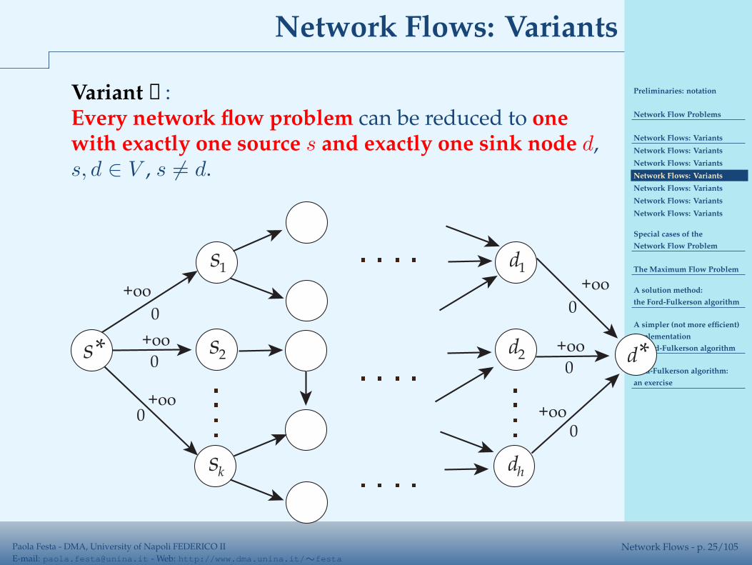
Variant ①:Every network flow problem can be reduced to onewith exactly one source s and exactly one sink node d,s, d ∈ V , s 6= d.
Let us suppose that N = (V,A) has k source nodess1, . . . , sk and h sink nodes d1, . . . , dh.

Preliminaries: notation
Network Flow Problems
Network Flows: Variants
Network Flows: Variants
Network Flows: Variants
Network Flows: Variants
Network Flows: Variants
Network Flows: Variants
Network Flows: Variants
Special cases of the
Network Flow Problem
The Maximum Flow Problem
A solution method:
the Ford-Fulkerson algorithm
A simpler (not more efficient)
implementation
of Ford-Fulkerson algorithm
Ford-Fulkerson algorithm:
an exercise
Paola Festa - DMA, University of Napoli FEDERICO II
E-mail: [email protected] - Web: http://www.dma.unina.it/∼festaNetwork Flows - p. 24/105
Network Flows: Variants
Variant ①:Every network flow problem can be reduced to onewith exactly one source s and exactly one sink node d,s, d ∈ V , s 6= d.
Let us suppose that N = (V,A) has k source nodess1, . . . , sk and h sink nodes d1, . . . , dh.
It is always possible to define
✍ a dummy source s∗ and a dummy sink d∗;
✍ k dummy arcs (s∗, sq) (q = 1, . . . , k);
✍ h dummy arcs (dl, d∗) (l = 1, . . . , h) s.t.
∀ q = 1, . . . , k,
{
ks∗sq= +∞;
cs∗sq= 0.
∀ l = 1, . . . , h,
{
kdld∗ = +∞;
cdld∗ = 0.
Preliminaries: notation
Network Flow Problems
Network Flows: Variants
Network Flows: Variants
Network Flows: Variants
Network Flows: Variants
Network Flows: Variants
Network Flows: Variants
Network Flows: Variants
Special cases of the
Network Flow Problem
The Maximum Flow Problem
A solution method:
the Ford-Fulkerson algorithm
A simpler (not more efficient)
implementation
of Ford-Fulkerson algorithm
Ford-Fulkerson algorithm:
an exercise
Paola Festa - DMA, University of Napoli FEDERICO II
E-mail: [email protected] - Web: http://www.dma.unina.it/∼festaNetwork Flows - p. 25/105
Network Flows: Variants
Variant ①:Every network flow problem can be reduced to onewith exactly one source s and exactly one sink node d,s, d ∈ V , s 6= d.
0
s*
s1
s2
sk
0
0
+oo
+oo
+oo
d*
d1
d2
dh
0
0
+oo
+oo
+oo0
Preliminaries: notation
Network Flow Problems
Network Flows: Variants
Network Flows: Variants
Network Flows: Variants
Network Flows: Variants
Network Flows: Variants
Network Flows: Variants
Network Flows: Variants
Special cases of the
Network Flow Problem
The Maximum Flow Problem
A solution method:
the Ford-Fulkerson algorithm
A simpler (not more efficient)
implementation
of Ford-Fulkerson algorithm
Ford-Fulkerson algorithm:
an exercise
Paola Festa - DMA, University of Napoli FEDERICO II
E-mail: [email protected] - Web: http://www.dma.unina.it/∼festaNetwork Flows - p. 26/105
Network Flows: Variants
Variant ②:Every network flow problem can be reduced to onewithout sources or sinks (bi = 0, ∀ i ∈ V , circulationproblems).
Without loss of generality, consider a networkN = (V,A) with a single source node s and a singlesink node d.
Preliminaries: notation
Network Flow Problems
Network Flows: Variants
Network Flows: Variants
Network Flows: Variants
Network Flows: Variants
Network Flows: Variants
Network Flows: Variants
Network Flows: Variants
Special cases of the
Network Flow Problem
The Maximum Flow Problem
A solution method:
the Ford-Fulkerson algorithm
A simpler (not more efficient)
implementation
of Ford-Fulkerson algorithm
Ford-Fulkerson algorithm:
an exercise
Paola Festa - DMA, University of Napoli FEDERICO II
E-mail: [email protected] - Web: http://www.dma.unina.it/∼festaNetwork Flows - p. 26/105
Network Flows: Variants
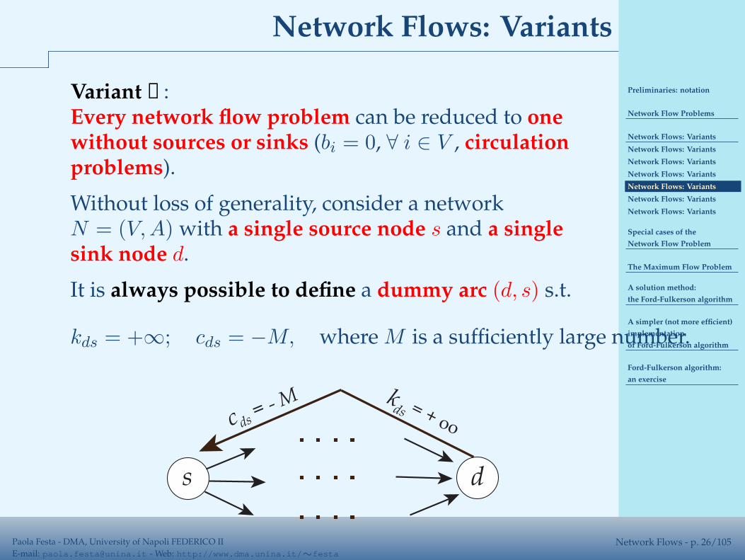
Variant ②:Every network flow problem can be reduced to onewithout sources or sinks (bi = 0, ∀ i ∈ V , circulationproblems).
Without loss of generality, consider a networkN = (V,A) with a single source node s and a singlesink node d.
It is always possible to define a dummy arc (d, s) s.t.
kds = +∞; cds = −M, where M is a sufficiently large number.
s
= - M
d
= + oo
kdsc ds
Preliminaries: notation
Network Flow Problems
Network Flows: Variants
Network Flows: Variants
Network Flows: Variants
Network Flows: Variants
Network Flows: Variants
Network Flows: Variants
Network Flows: Variants
Special cases of the
Network Flow Problem
The Maximum Flow Problem
A solution method:
the Ford-Fulkerson algorithm
A simpler (not more efficient)
implementation
of Ford-Fulkerson algorithm
Ford-Fulkerson algorithm:
an exercise
Paola Festa - DMA, University of Napoli FEDERICO II
E-mail: [email protected] - Web: http://www.dma.unina.it/∼festaNetwork Flows - p. 27/105
Network Flows: Variants
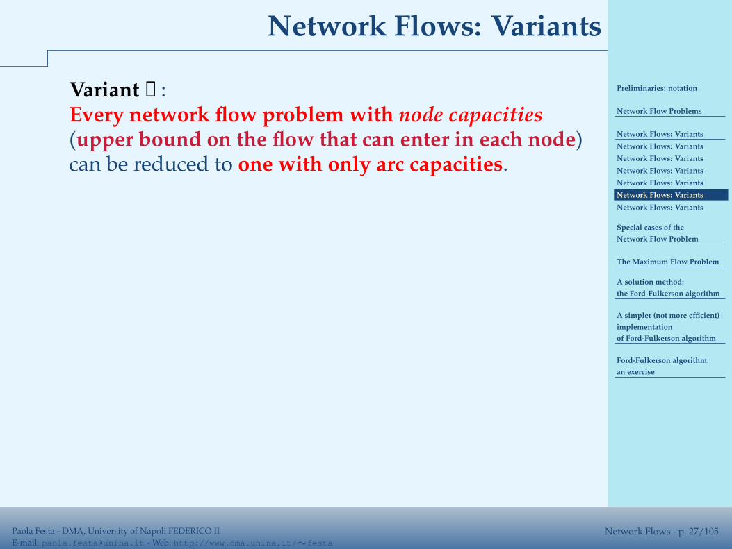
Variant ③:Every network flow problem with node capacities(upper bound on the flow that can enter in each node)can be reduced to one with only arc capacities.
Preliminaries: notation
Network Flow Problems
Network Flows: Variants
Network Flows: Variants
Network Flows: Variants
Network Flows: Variants
Network Flows: Variants
Network Flows: Variants
Network Flows: Variants
Special cases of the
Network Flow Problem
The Maximum Flow Problem
A solution method:
the Ford-Fulkerson algorithm
A simpler (not more efficient)
implementation
of Ford-Fulkerson algorithm
Ford-Fulkerson algorithm:
an exercise
Paola Festa - DMA, University of Napoli FEDERICO II
E-mail: [email protected] - Web: http://www.dma.unina.it/∼festaNetwork Flows - p. 27/105
Network Flows: Variants
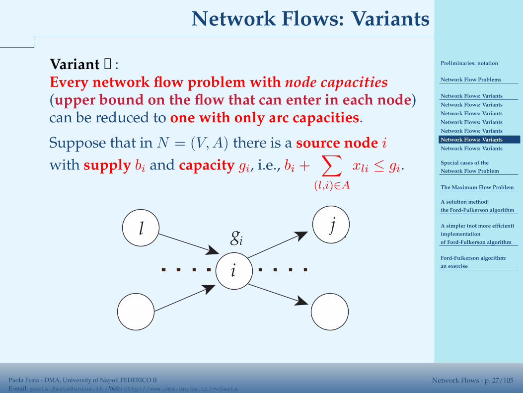
Variant ③:Every network flow problem with node capacities(upper bound on the flow that can enter in each node)can be reduced to one with only arc capacities.
Suppose that in N = (V,A) there is a source node i
with supply bi and capacity gi, i.e., bi +∑
(l,i)∈A
xli ≤ gi.
i
l jgi
Preliminaries: notation
Network Flow Problems
Network Flows: Variants
Network Flows: Variants
Network Flows: Variants
Network Flows: Variants
Network Flows: Variants
Network Flows: Variants
Network Flows: Variants
Special cases of the
Network Flow Problem
The Maximum Flow Problem
A solution method:
the Ford-Fulkerson algorithm
A simpler (not more efficient)
implementation
of Ford-Fulkerson algorithm
Ford-Fulkerson algorithm:
an exercise
Paola Festa - DMA, University of Napoli FEDERICO II
E-mail: [email protected] - Web: http://www.dma.unina.it/∼festaNetwork Flows - p. 28/105
Network Flows: Variants
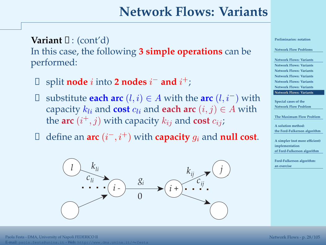
Variant ③: (cont’d)In this case, the following 3 simple operations can beperformed:
❶ split node i into 2 nodes i− and i+;
❷ substitute each arc (l, i) ∈ A with the arc (l, i−) withcapacity kli and cost cli and each arc (i, j) ∈ A withthe arc (i+, j) with capacity kij and cost cij ;
❸ define an arc (i−, i+) with capacity gi and null cost.
i -
l j
i +0
gi
kli
cli
kijcij
Preliminaries: notation
Network Flow Problems
Network Flows: Variants
Special cases of the
Network Flow Problem
Special Network Flows, ➀
Special Network Flows, ➁
Special Network Flows, ➂
The Maximum Flow Problem
A solution method:
the Ford-Fulkerson algorithm
A simpler (not more efficient)
implementation
of Ford-Fulkerson algorithm
Ford-Fulkerson algorithm:
an exercise
Paola Festa - DMA, University of Napoli FEDERICO II
E-mail: [email protected] - Web: http://www.dma.unina.it/∼festaNetwork Flows - p. 29/105
Special cases of theNetwork Flow Problem
Preliminaries: notation
Network Flow Problems
Network Flows: Variants
Special cases of the
Network Flow Problem
Special Network Flows, ➀
Special Network Flows, ➁
Special Network Flows, ➂
The Maximum Flow Problem
A solution method:
the Ford-Fulkerson algorithm
A simpler (not more efficient)
implementation
of Ford-Fulkerson algorithm
Ford-Fulkerson algorithm:
an exercise
Paola Festa - DMA, University of Napoli FEDERICO II
E-mail: [email protected] - Web: http://www.dma.unina.it/∼festaNetwork Flows - p. 30/105
Special Network Flows, ➀
Special cases of the network flow problem areimportant and classical optimization problems,among them
✔ the transportation problem;
✔ the assignment problem;
✔ the shortest path problems (under a certainassumption on the arc costs);
✔ the maximum flow problem;
✔ ...
Preliminaries: notation
Network Flow Problems
Network Flows: Variants
Special cases of the
Network Flow Problem
Special Network Flows, ➀
Special Network Flows, ➁
Special Network Flows, ➂
The Maximum Flow Problem
A solution method:
the Ford-Fulkerson algorithm
A simpler (not more efficient)
implementation
of Ford-Fulkerson algorithm
Ford-Fulkerson algorithm:
an exercise
Paola Festa - DMA, University of Napoli FEDERICO II
E-mail: [email protected] - Web: http://www.dma.unina.it/∼festaNetwork Flows - p. 31/105
Special Network Flows, ➁
The shortest path problem under the assumption thatcij ≥ 0, ∀ (i, j) ∈ A, or that there are no negative cycles.

Preliminaries: notation
Network Flow Problems
Network Flows: Variants
Special cases of the
Network Flow Problem
Special Network Flows, ➀
Special Network Flows, ➁
Special Network Flows, ➂
The Maximum Flow Problem
A solution method:
the Ford-Fulkerson algorithm
A simpler (not more efficient)
implementation
of Ford-Fulkerson algorithm
Ford-Fulkerson algorithm:
an exercise
Paola Festa - DMA, University of Napoli FEDERICO II
E-mail: [email protected] - Web: http://www.dma.unina.it/∼festaNetwork Flows - p. 31/105
Special Network Flows, ➁
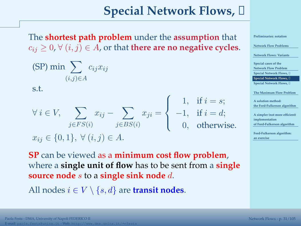
The shortest path problem under the assumption thatcij ≥ 0, ∀ (i, j) ∈ A, or that there are no negative cycles.
(SP) min∑
(i,j)∈A
cijxij
s.t.
∀ i ∈ V,∑
j∈FS(i)
xij −∑
j∈BS(i)
xji =
1, if i = s;
−1, if i = d;
0, otherwise.
xij ∈ {0, 1}, ∀ (i, j) ∈ A.
Preliminaries: notation
Network Flow Problems
Network Flows: Variants
Special cases of the
Network Flow Problem
Special Network Flows, ➀
Special Network Flows, ➁
Special Network Flows, ➂
The Maximum Flow Problem
A solution method:
the Ford-Fulkerson algorithm
A simpler (not more efficient)
implementation
of Ford-Fulkerson algorithm
Ford-Fulkerson algorithm:
an exercise
Paola Festa - DMA, University of Napoli FEDERICO II
E-mail: [email protected] - Web: http://www.dma.unina.it/∼festaNetwork Flows - p. 31/105
Special Network Flows, ➁
The shortest path problem under the assumption thatcij ≥ 0, ∀ (i, j) ∈ A, or that there are no negative cycles.
(SP) min∑
(i,j)∈A
cijxij
s.t.
∀ i ∈ V,∑
j∈FS(i)
xij −∑
j∈BS(i)
xji =
1, if i = s;
−1, if i = d;
0, otherwise.
xij ∈ {0, 1}, ∀ (i, j) ∈ A.
SP can be viewed as a minimum cost flow problem,where a single unit of flow has to be sent from a singlesource node s to a single sink node d.
All nodes i ∈ V \ {s, d} are transit nodes.
Preliminaries: notation
Network Flow Problems
Network Flows: Variants
Special cases of the
Network Flow Problem
Special Network Flows, ➀
Special Network Flows, ➁
Special Network Flows, ➂
The Maximum Flow Problem
A solution method:
the Ford-Fulkerson algorithm
A simpler (not more efficient)
implementation
of Ford-Fulkerson algorithm
Ford-Fulkerson algorithm:
an exercise
Paola Festa - DMA, University of Napoli FEDERICO II
E-mail: [email protected] - Web: http://www.dma.unina.it/∼festaNetwork Flows - p. 32/105
Special Network Flows, ➂
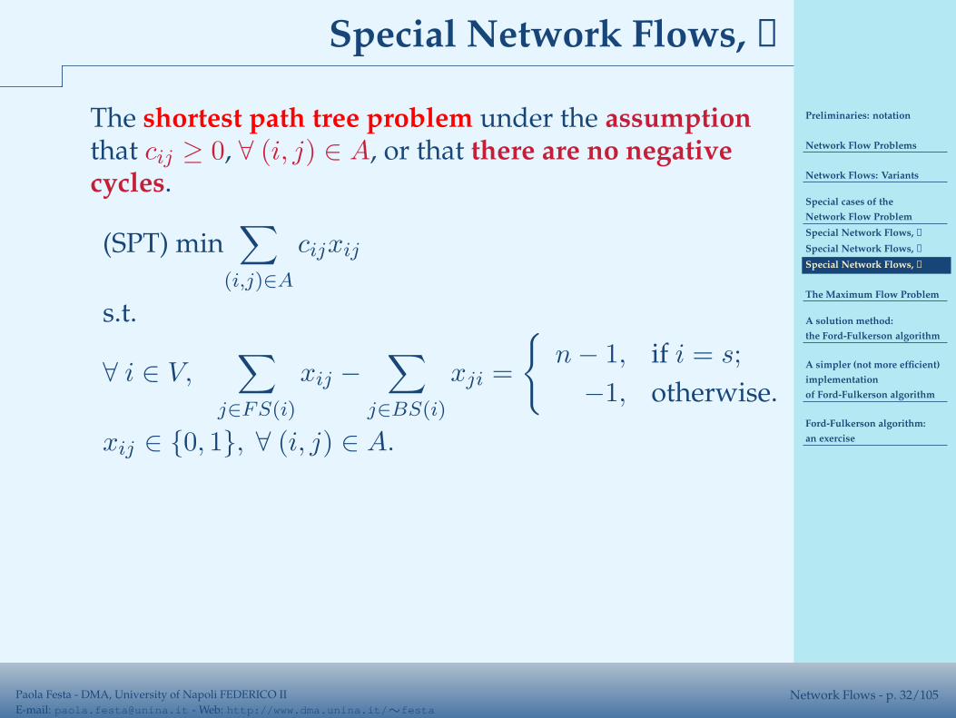
The shortest path tree problem under the assumptionthat cij ≥ 0, ∀ (i, j) ∈ A, or that there are no negativecycles.
(SPT) min∑
(i,j)∈A
cijxij
s.t.
∀ i ∈ V,∑
j∈FS(i)
xij −∑
j∈BS(i)
xji =
{
n − 1, if i = s;
−1, otherwise.
xij ∈ {0, 1}, ∀ (i, j) ∈ A.
Preliminaries: notation
Network Flow Problems
Network Flows: Variants
Special cases of the
Network Flow Problem
Special Network Flows, ➀
Special Network Flows, ➁
Special Network Flows, ➂
The Maximum Flow Problem
A solution method:
the Ford-Fulkerson algorithm
A simpler (not more efficient)
implementation
of Ford-Fulkerson algorithm
Ford-Fulkerson algorithm:
an exercise
Paola Festa - DMA, University of Napoli FEDERICO II
E-mail: [email protected] - Web: http://www.dma.unina.it/∼festaNetwork Flows - p. 32/105
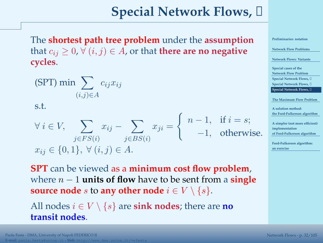
Special Network Flows, ➂
The shortest path tree problem under the assumptionthat cij ≥ 0, ∀ (i, j) ∈ A, or that there are no negativecycles.
(SPT) min∑
(i,j)∈A
cijxij
s.t.
∀ i ∈ V,∑
j∈FS(i)
xij −∑
j∈BS(i)
xji =
{
n − 1, if i = s;
−1, otherwise.
xij ∈ {0, 1}, ∀ (i, j) ∈ A.
SPT can be viewed as a minimum cost flow problem,where n − 1 units of flow have to be sent from a singlesource node s to any other node i ∈ V \ {s}.
All nodes i ∈ V \ {s} are sink nodes; there are notransit nodes.

Preliminaries: notation
Network Flow Problems
Network Flows: Variants
Special cases of the
Network Flow Problem
The Maximum Flow Problem
Definition
MF as MCF, ➀
MF as MCF, ➁
Math formulation, ➀
Math formulation, ➁
Math formulation, ➂
Math formulation, ➃
Properties, ➀
Properties, ➁
Properties, ➂
Properties, ➃
Properties, ➃
Properties, ➃
Properties, ➃
Properties, ➃
Properties, ➃
Properties, ➄
Max Flow / Min Cut, ➀
Max Flow / Min Cut, ➁
Satured and unloading arcs
Residual network, ➀
Residual network, ➀
Residual network, ➁
Residual network, ➁
Augmenting path
Optimality conditions, ➀
Optimality conditions, ➁
Optimality conditions, ➁
Optimality conditions, ➁
A solution method:
Paola Festa - DMA, University of Napoli FEDERICO II
E-mail: [email protected] - Web: http://www.dma.unina.it/∼festaNetwork Flows - p. 33/105
The Maximum Flow Problem
Preliminaries: notation
Network Flow Problems
Network Flows: Variants
Special cases of the
Network Flow Problem
The Maximum Flow Problem
Definition
MF as MCF, ➀
MF as MCF, ➁
Math formulation, ➀
Math formulation, ➁
Math formulation, ➂
Math formulation, ➃
Properties, ➀
Properties, ➁
Properties, ➂
Properties, ➃
Properties, ➃
Properties, ➃
Properties, ➃
Properties, ➃
Properties, ➃
Properties, ➄
Max Flow / Min Cut, ➀
Max Flow / Min Cut, ➁
Satured and unloading arcs
Residual network, ➀
Residual network, ➀
Residual network, ➁
Residual network, ➁
Augmenting path
Optimality conditions, ➀
Optimality conditions, ➁
Optimality conditions, ➁
Optimality conditions, ➁
A solution method:
Paola Festa - DMA, University of Napoli FEDERICO II
E-mail: [email protected] - Web: http://www.dma.unina.it/∼festaNetwork Flows - p. 34/105
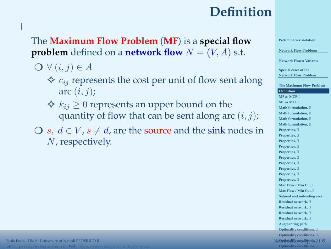
Definition
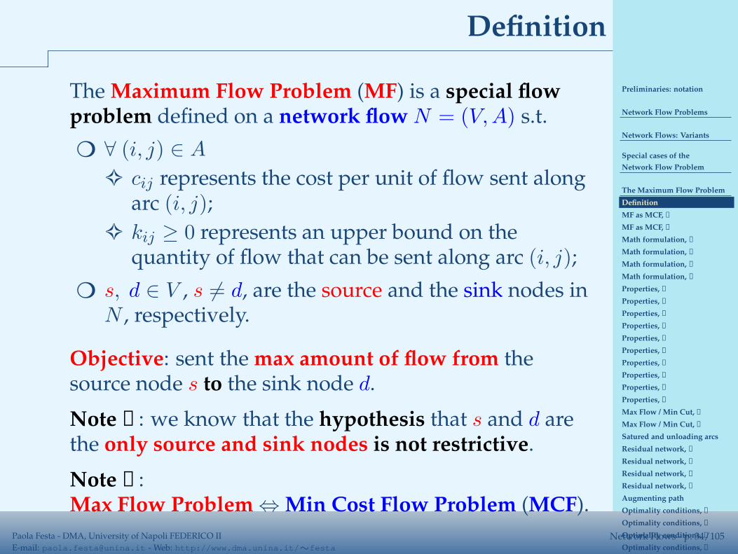
The Maximum Flow Problem (MF) is a special flowproblem defined on a network flow N = (V,A) s.t.
❍ ∀ (i, j) ∈ A
✧ cij represents the cost per unit of flow sent alongarc (i, j);
✧ kij ≥ 0 represents an upper bound on thequantity of flow that can be sent along arc (i, j);
❍ s, d ∈ V , s 6= d, are the source and the sink nodes inN , respectively.
Preliminaries: notation
Network Flow Problems
Network Flows: Variants
Special cases of the
Network Flow Problem
The Maximum Flow Problem
Definition
MF as MCF, ➀
MF as MCF, ➁
Math formulation, ➀
Math formulation, ➁
Math formulation, ➂
Math formulation, ➃
Properties, ➀
Properties, ➁
Properties, ➂
Properties, ➃
Properties, ➃
Properties, ➃
Properties, ➃
Properties, ➃
Properties, ➃
Properties, ➄
Max Flow / Min Cut, ➀
Max Flow / Min Cut, ➁
Satured and unloading arcs
Residual network, ➀
Residual network, ➀
Residual network, ➁
Residual network, ➁
Augmenting path
Optimality conditions, ➀
Optimality conditions, ➁
Optimality conditions, ➁
Optimality conditions, ➁
A solution method:
Paola Festa - DMA, University of Napoli FEDERICO II
E-mail: [email protected] - Web: http://www.dma.unina.it/∼festaNetwork Flows - p. 34/105
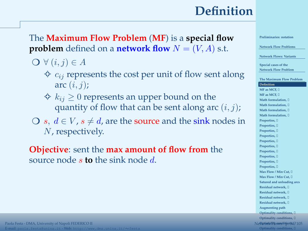
Definition
The Maximum Flow Problem (MF) is a special flowproblem defined on a network flow N = (V,A) s.t.
❍ ∀ (i, j) ∈ A
✧ cij represents the cost per unit of flow sent alongarc (i, j);
✧ kij ≥ 0 represents an upper bound on thequantity of flow that can be sent along arc (i, j);
❍ s, d ∈ V , s 6= d, are the source and the sink nodes inN , respectively.
Objective: sent the max amount of flow from thesource node s to the sink node d.
Preliminaries: notation
Network Flow Problems
Network Flows: Variants
Special cases of the
Network Flow Problem
The Maximum Flow Problem
Definition
MF as MCF, ➀
MF as MCF, ➁
Math formulation, ➀
Math formulation, ➁
Math formulation, ➂
Math formulation, ➃
Properties, ➀
Properties, ➁
Properties, ➂
Properties, ➃
Properties, ➃
Properties, ➃
Properties, ➃
Properties, ➃
Properties, ➃
Properties, ➄
Max Flow / Min Cut, ➀
Max Flow / Min Cut, ➁
Satured and unloading arcs
Residual network, ➀
Residual network, ➀
Residual network, ➁
Residual network, ➁
Augmenting path
Optimality conditions, ➀
Optimality conditions, ➁
Optimality conditions, ➁
Optimality conditions, ➁
A solution method:
Paola Festa - DMA, University of Napoli FEDERICO II
E-mail: [email protected] - Web: http://www.dma.unina.it/∼festaNetwork Flows - p. 34/105
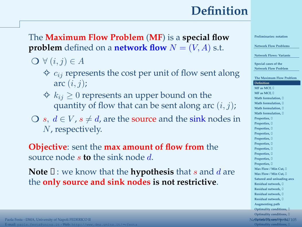
Definition
The Maximum Flow Problem (MF) is a special flowproblem defined on a network flow N = (V,A) s.t.
❍ ∀ (i, j) ∈ A
✧ cij represents the cost per unit of flow sent alongarc (i, j);
✧ kij ≥ 0 represents an upper bound on thequantity of flow that can be sent along arc (i, j);
❍ s, d ∈ V , s 6= d, are the source and the sink nodes inN , respectively.
Objective: sent the max amount of flow from thesource node s to the sink node d.
Note ①: we know that the hypothesis that s and d arethe only source and sink nodes is not restrictive.
Preliminaries: notation
Network Flow Problems
Network Flows: Variants
Special cases of the
Network Flow Problem
The Maximum Flow Problem
Definition
MF as MCF, ➀
MF as MCF, ➁
Math formulation, ➀
Math formulation, ➁
Math formulation, ➂
Math formulation, ➃
Properties, ➀
Properties, ➁
Properties, ➂
Properties, ➃
Properties, ➃
Properties, ➃
Properties, ➃
Properties, ➃
Properties, ➃
Properties, ➄
Max Flow / Min Cut, ➀
Max Flow / Min Cut, ➁
Satured and unloading arcs
Residual network, ➀
Residual network, ➀
Residual network, ➁
Residual network, ➁
Augmenting path
Optimality conditions, ➀
Optimality conditions, ➁
Optimality conditions, ➁
Optimality conditions, ➁
A solution method:
Paola Festa - DMA, University of Napoli FEDERICO II
E-mail: [email protected] - Web: http://www.dma.unina.it/∼festaNetwork Flows - p. 34/105
Definition
The Maximum Flow Problem (MF) is a special flowproblem defined on a network flow N = (V,A) s.t.
❍ ∀ (i, j) ∈ A
✧ cij represents the cost per unit of flow sent alongarc (i, j);
✧ kij ≥ 0 represents an upper bound on thequantity of flow that can be sent along arc (i, j);
❍ s, d ∈ V , s 6= d, are the source and the sink nodes inN , respectively.
Objective: sent the max amount of flow from thesource node s to the sink node d.
Note ①: we know that the hypothesis that s and d arethe only source and sink nodes is not restrictive.
Note ②:Max Flow Problem ⇔ Min Cost Flow Problem (MCF).
Preliminaries: notation
Network Flow Problems
Network Flows: Variants
Special cases of the
Network Flow Problem
The Maximum Flow Problem
Definition
MF as MCF, ➀
MF as MCF, ➁
Math formulation, ➀
Math formulation, ➁
Math formulation, ➂
Math formulation, ➃
Properties, ➀
Properties, ➁
Properties, ➂
Properties, ➃
Properties, ➃
Properties, ➃
Properties, ➃
Properties, ➃
Properties, ➃
Properties, ➄
Max Flow / Min Cut, ➀
Max Flow / Min Cut, ➁
Satured and unloading arcs
Residual network, ➀
Residual network, ➀
Residual network, ➁
Residual network, ➁
Augmenting path
Optimality conditions, ➀
Optimality conditions, ➁
Optimality conditions, ➁
Optimality conditions, ➁
A solution method:
Paola Festa - DMA, University of Napoli FEDERICO II
E-mail: [email protected] - Web: http://www.dma.unina.it/∼festaNetwork Flows - p. 35/105
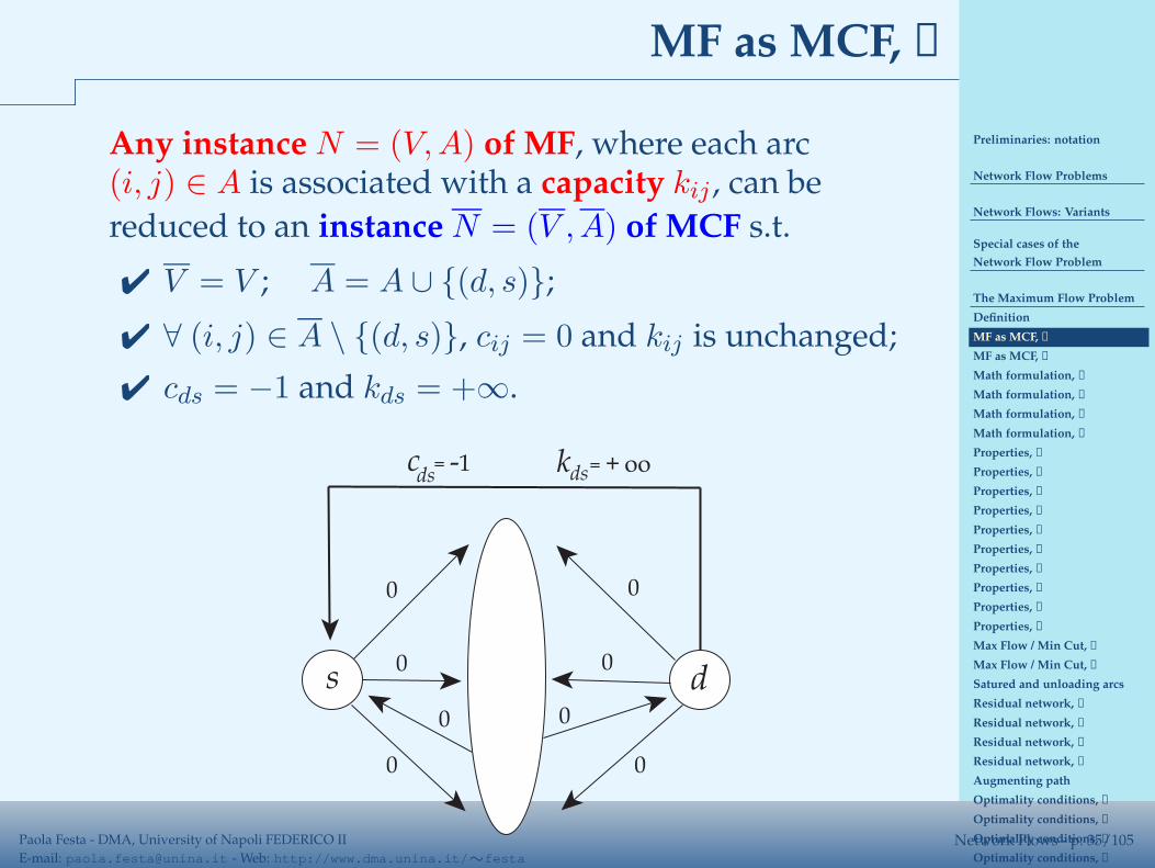
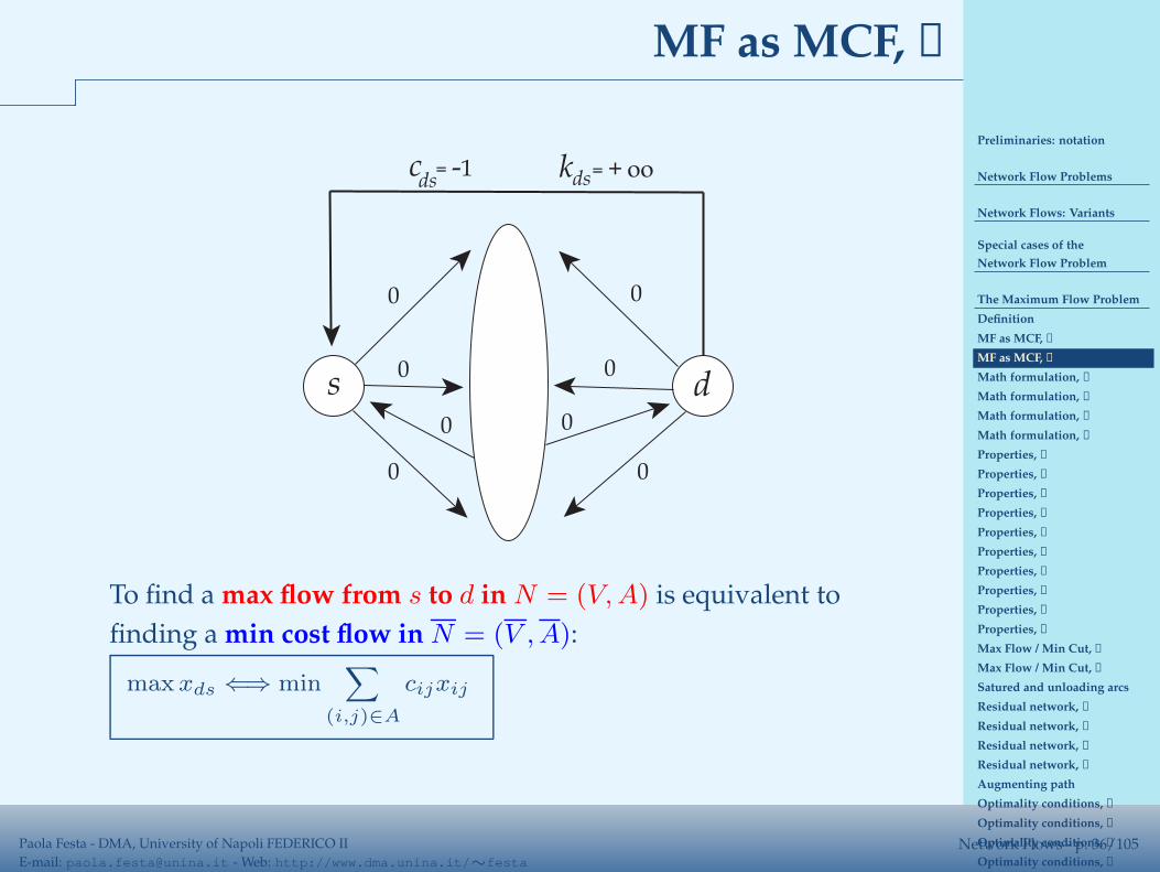
MF as MCF, ➀
Any instance N = (V,A) of MF, where each arc(i, j) ∈ A is associated with a capacity kij , can be
reduced to an instance N = (V ,A) of MCF s.t.
✔ V = V ; A = A ∪ {(d, s)};
✔ ∀ (i, j) ∈ A \ {(d, s)}, cij = 0 and kij is unchanged;
✔ cds = −1 and kds = +∞.
s0
d
0
0
0
0
0
k = + ooc = -1
0 0
ds ds
Preliminaries: notation
Network Flow Problems
Network Flows: Variants
Special cases of the
Network Flow Problem
The Maximum Flow Problem
Definition
MF as MCF, ➀
MF as MCF, ➁
Math formulation, ➀
Math formulation, ➁
Math formulation, ➂
Math formulation, ➃
Properties, ➀
Properties, ➁
Properties, ➂
Properties, ➃
Properties, ➃
Properties, ➃
Properties, ➃
Properties, ➃
Properties, ➃
Properties, ➄
Max Flow / Min Cut, ➀
Max Flow / Min Cut, ➁
Satured and unloading arcs
Residual network, ➀
Residual network, ➀
Residual network, ➁
Residual network, ➁
Augmenting path
Optimality conditions, ➀
Optimality conditions, ➁
Optimality conditions, ➁
Optimality conditions, ➁
A solution method:
Paola Festa - DMA, University of Napoli FEDERICO II
E-mail: [email protected] - Web: http://www.dma.unina.it/∼festaNetwork Flows - p. 36/105
MF as MCF, ➁
s0
d
0
0
0
0
0
k = + ooc = -1
0 0
ds ds
To find a max flow from s to d in N = (V, A) is equivalent to
finding a min cost flow in N = (V , A):
max xds ⇐⇒ min∑
(i,j)∈A
cijxij
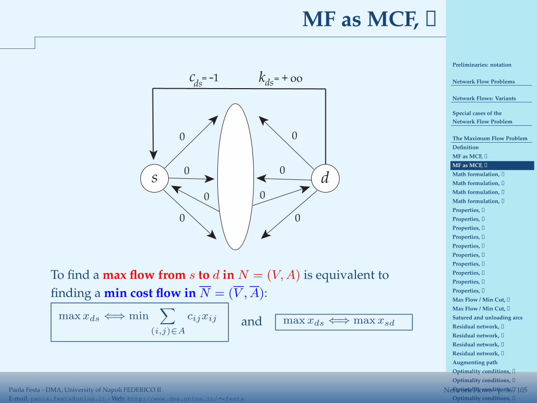
Preliminaries: notation
Network Flow Problems
Network Flows: Variants
Special cases of the
Network Flow Problem
The Maximum Flow Problem
Definition
MF as MCF, ➀
MF as MCF, ➁
Math formulation, ➀
Math formulation, ➁
Math formulation, ➂
Math formulation, ➃
Properties, ➀
Properties, ➁
Properties, ➂
Properties, ➃
Properties, ➃
Properties, ➃
Properties, ➃
Properties, ➃
Properties, ➃
Properties, ➄
Max Flow / Min Cut, ➀
Max Flow / Min Cut, ➁
Satured and unloading arcs
Residual network, ➀
Residual network, ➀
Residual network, ➁
Residual network, ➁
Augmenting path
Optimality conditions, ➀
Optimality conditions, ➁
Optimality conditions, ➁
Optimality conditions, ➁
A solution method:
Paola Festa - DMA, University of Napoli FEDERICO II
E-mail: [email protected] - Web: http://www.dma.unina.it/∼festaNetwork Flows - p. 36/105
MF as MCF, ➁
s0
d
0
0
0
0
0
k = + ooc = -1
0 0
ds ds
To find a max flow from s to d in N = (V, A) is equivalent to
finding a min cost flow in N = (V , A):
max xds ⇐⇒ min∑
(i,j)∈A
cijxij and max xds ⇐⇒ max xsd
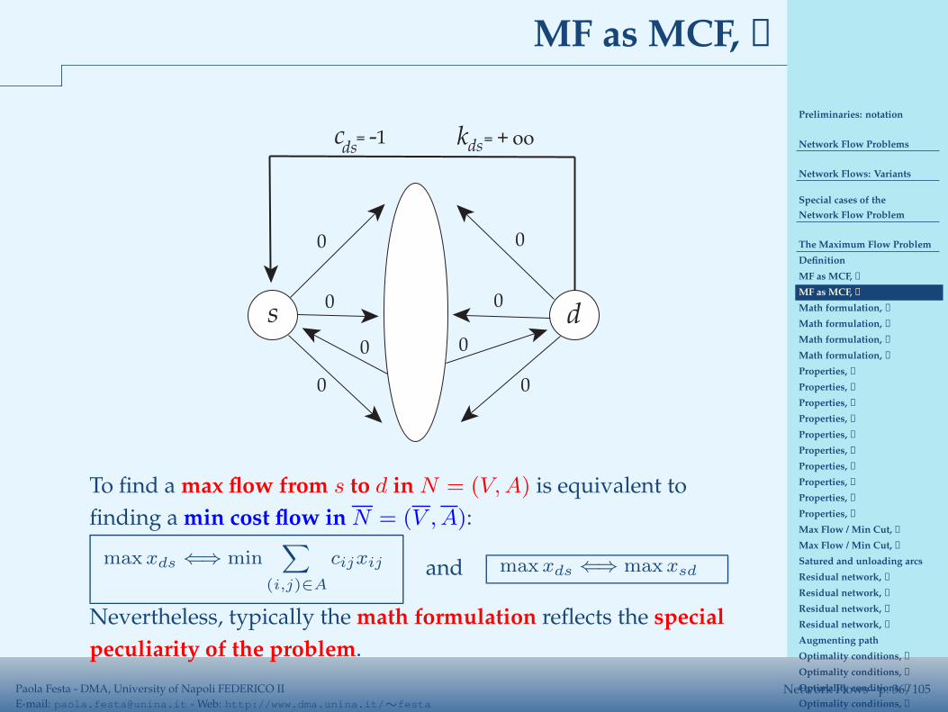
Nevertheless, typically the math formulation reflects the special
peculiarity of the problem.
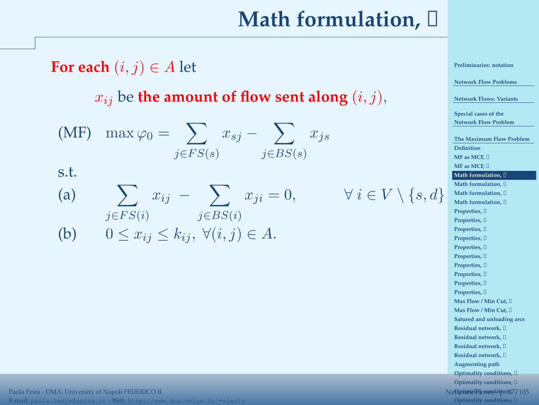
Preliminaries: notation
Network Flow Problems
Network Flows: Variants
Special cases of the
Network Flow Problem
The Maximum Flow Problem
Definition
MF as MCF, ➀
MF as MCF, ➁
Math formulation, ➀
Math formulation, ➁
Math formulation, ➂
Math formulation, ➃
Properties, ➀
Properties, ➁
Properties, ➂
Properties, ➃
Properties, ➃
Properties, ➃
Properties, ➃
Properties, ➃
Properties, ➃
Properties, ➄
Max Flow / Min Cut, ➀
Max Flow / Min Cut, ➁
Satured and unloading arcs
Residual network, ➀
Residual network, ➀
Residual network, ➁
Residual network, ➁
Augmenting path
Optimality conditions, ➀
Optimality conditions, ➁
Optimality conditions, ➁
Optimality conditions, ➁
A solution method:
Paola Festa - DMA, University of Napoli FEDERICO II
E-mail: [email protected] - Web: http://www.dma.unina.it/∼festaNetwork Flows - p. 37/105
Math formulation, ➀
For each (i, j) ∈ A let
xij be the amount of flow sent along (i, j),
(MF) max ϕ0 =∑
j∈FS(s)
xsj −∑
j∈BS(s)
xjs
s.t.
(a)∑
j∈FS(i)
xij −∑
j∈BS(i)
xji = 0, ∀ i ∈ V \ {s, d}
(b) 0 ≤ xij ≤ kij , ∀(i, j) ∈ A.
Note ①: if BS(s) = ∅, the o.f. reduces to
max ϕ0 =∑
j∈FS(s)
xsj .
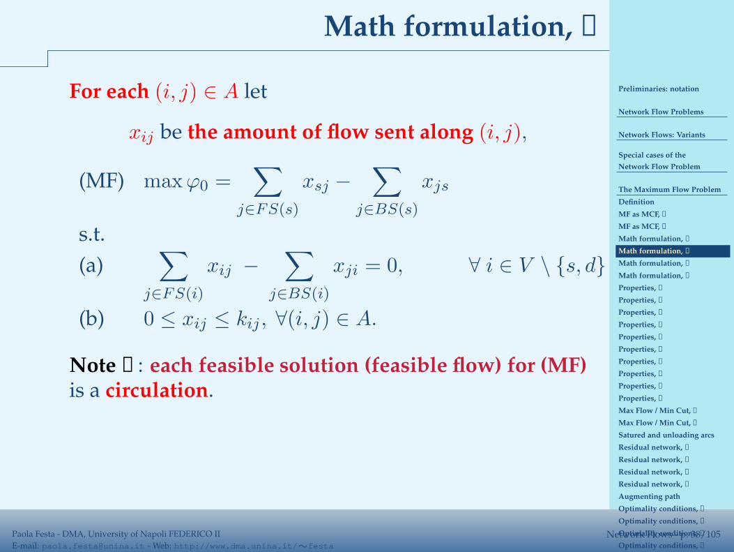
Preliminaries: notation
Network Flow Problems
Network Flows: Variants
Special cases of the
Network Flow Problem
The Maximum Flow Problem
Definition
MF as MCF, ➀
MF as MCF, ➁
Math formulation, ➀
Math formulation, ➁
Math formulation, ➂
Math formulation, ➃
Properties, ➀
Properties, ➁
Properties, ➂
Properties, ➃
Properties, ➃
Properties, ➃
Properties, ➃
Properties, ➃
Properties, ➃
Properties, ➄
Max Flow / Min Cut, ➀
Max Flow / Min Cut, ➁
Satured and unloading arcs
Residual network, ➀
Residual network, ➀
Residual network, ➁
Residual network, ➁
Augmenting path
Optimality conditions, ➀
Optimality conditions, ➁
Optimality conditions, ➁
Optimality conditions, ➁
A solution method:
Paola Festa - DMA, University of Napoli FEDERICO II
E-mail: [email protected] - Web: http://www.dma.unina.it/∼festaNetwork Flows - p. 38/105
Math formulation, ➁
For each (i, j) ∈ A let
xij be the amount of flow sent along (i, j),
(MF) max ϕ0 =∑
j∈FS(s)
xsj −∑
j∈BS(s)
xjs
s.t.
(a)∑
j∈FS(i)
xij −∑
j∈BS(i)
xji = 0, ∀ i ∈ V \ {s, d}
(b) 0 ≤ xij ≤ kij , ∀(i, j) ∈ A.
Note ②: each feasible solution (feasible flow) for (MF)is a circulation.
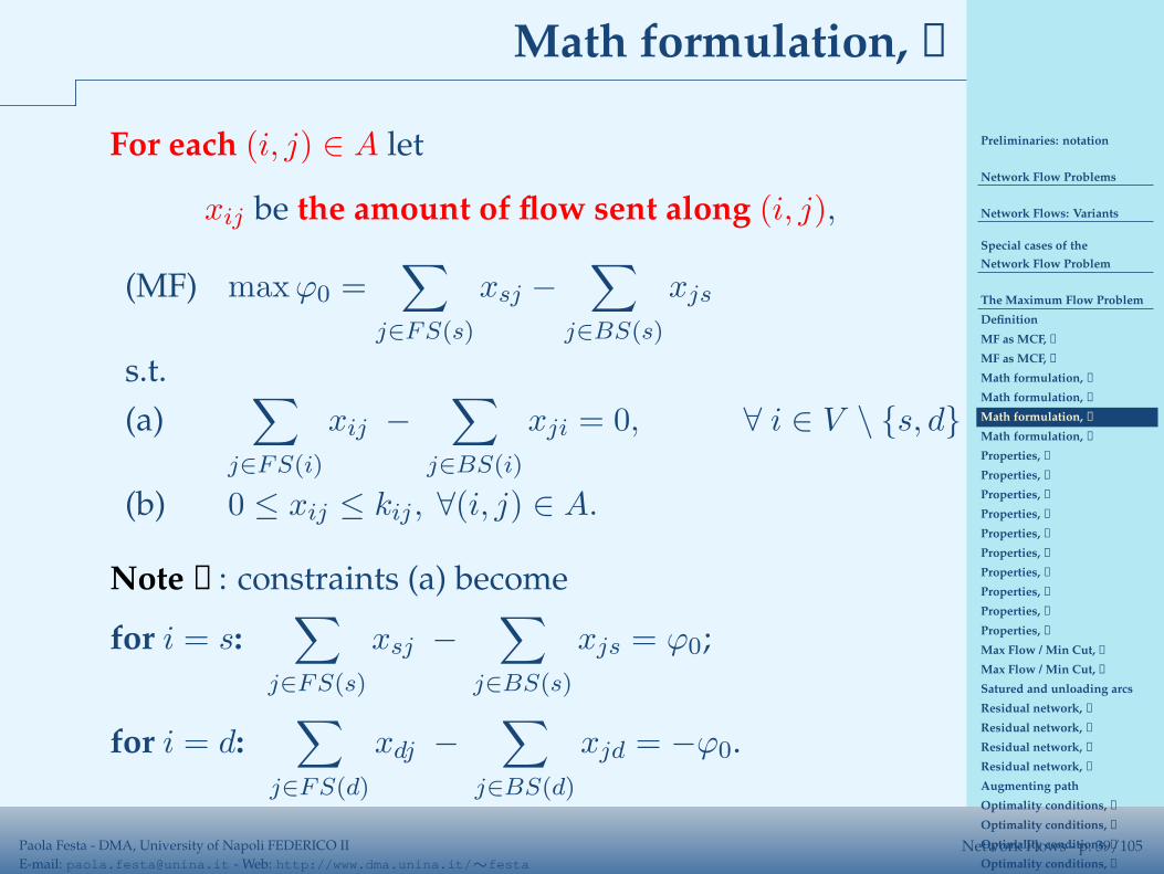
Preliminaries: notation
Network Flow Problems
Network Flows: Variants
Special cases of the
Network Flow Problem
The Maximum Flow Problem
Definition
MF as MCF, ➀
MF as MCF, ➁
Math formulation, ➀
Math formulation, ➁
Math formulation, ➂
Math formulation, ➃
Properties, ➀
Properties, ➁
Properties, ➂
Properties, ➃
Properties, ➃
Properties, ➃
Properties, ➃
Properties, ➃
Properties, ➃
Properties, ➄
Max Flow / Min Cut, ➀
Max Flow / Min Cut, ➁
Satured and unloading arcs
Residual network, ➀
Residual network, ➀
Residual network, ➁
Residual network, ➁
Augmenting path
Optimality conditions, ➀
Optimality conditions, ➁
Optimality conditions, ➁
Optimality conditions, ➁
A solution method:
Paola Festa - DMA, University of Napoli FEDERICO II
E-mail: [email protected] - Web: http://www.dma.unina.it/∼festaNetwork Flows - p. 39/105
Math formulation, ➂
For each (i, j) ∈ A let
xij be the amount of flow sent along (i, j),
(MF) max ϕ0 =∑
j∈FS(s)
xsj −∑
j∈BS(s)
xjs
s.t.
(a)∑
j∈FS(i)
xij −∑
j∈BS(i)
xji = 0, ∀ i ∈ V \ {s, d}
(b) 0 ≤ xij ≤ kij , ∀(i, j) ∈ A.
Note ③: constraints (a) become
for i = s:∑
j∈FS(s)
xsj −∑
j∈BS(s)
xjs = ϕ0;
for i = d:∑
j∈FS(d)
xdj −∑
j∈BS(d)
xjd = −ϕ0.
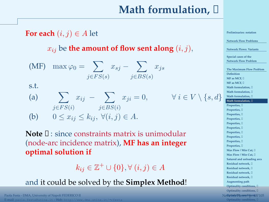
Preliminaries: notation
Network Flow Problems
Network Flows: Variants
Special cases of the
Network Flow Problem
The Maximum Flow Problem
Definition
MF as MCF, ➀
MF as MCF, ➁
Math formulation, ➀
Math formulation, ➁
Math formulation, ➂
Math formulation, ➃
Properties, ➀
Properties, ➁
Properties, ➂
Properties, ➃
Properties, ➃
Properties, ➃
Properties, ➃
Properties, ➃
Properties, ➃
Properties, ➄
Max Flow / Min Cut, ➀
Max Flow / Min Cut, ➁
Satured and unloading arcs
Residual network, ➀
Residual network, ➀
Residual network, ➁
Residual network, ➁
Augmenting path
Optimality conditions, ➀
Optimality conditions, ➁
Optimality conditions, ➁
Optimality conditions, ➁
A solution method:
Paola Festa - DMA, University of Napoli FEDERICO II
E-mail: [email protected] - Web: http://www.dma.unina.it/∼festaNetwork Flows - p. 40/105
Math formulation, ➃
For each (i, j) ∈ A let
xij be the amount of flow sent along (i, j),
(MF) max ϕ0 =∑
j∈FS(s)
xsj −∑
j∈BS(s)
xjs
s.t.
(a)∑
j∈FS(i)
xij −∑
j∈BS(i)
xji = 0, ∀ i ∈ V \ {s, d}
(b) 0 ≤ xij ≤ kij , ∀(i, j) ∈ A.
Note ④: since constraints matrix is unimodular(node-arc incidence matrix), MF has an integeroptimal solution if
kij ∈ Z+ ∪ {0},∀ (i, j) ∈ A
and it could be solved by the Simplex Method!
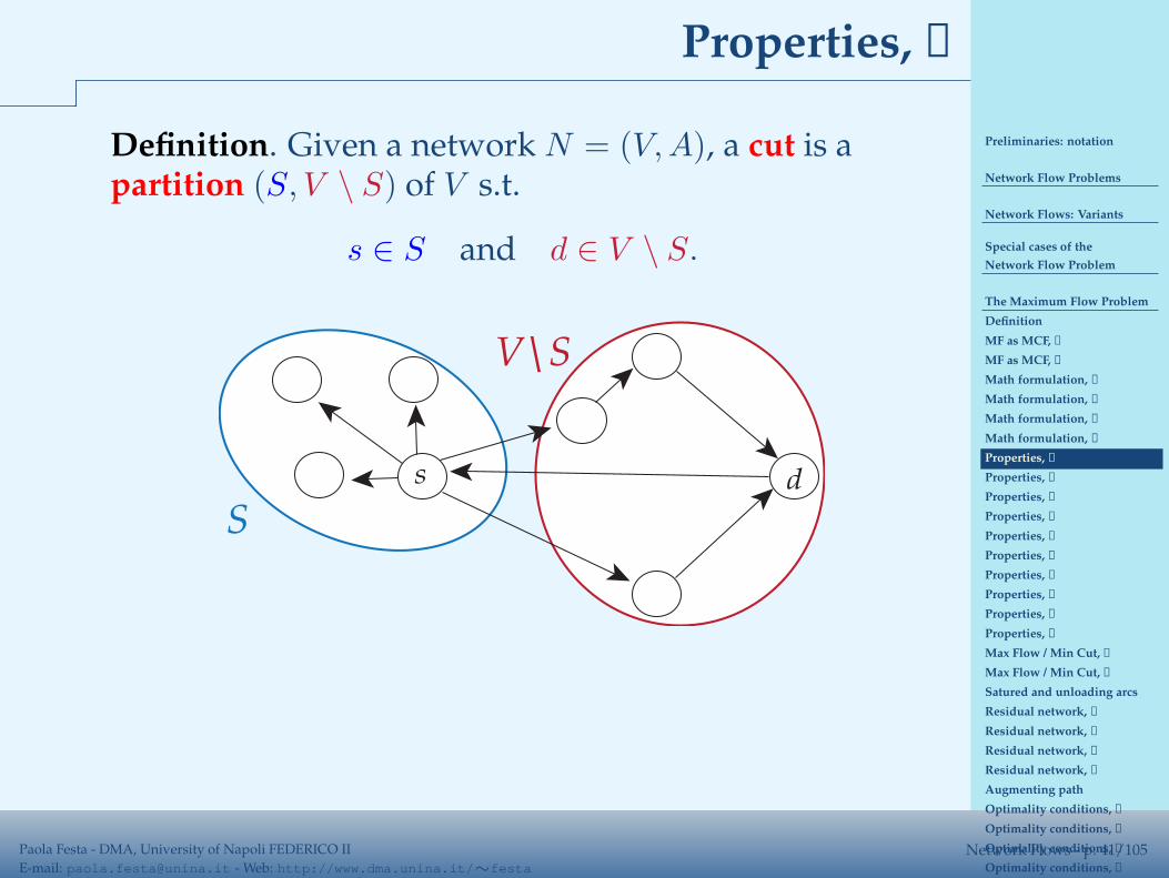
Preliminaries: notation
Network Flow Problems
Network Flows: Variants
Special cases of the
Network Flow Problem
The Maximum Flow Problem
Definition
MF as MCF, ➀
MF as MCF, ➁
Math formulation, ➀
Math formulation, ➁
Math formulation, ➂
Math formulation, ➃
Properties, ➀
Properties, ➁
Properties, ➂
Properties, ➃
Properties, ➃
Properties, ➃
Properties, ➃
Properties, ➃
Properties, ➃
Properties, ➄
Max Flow / Min Cut, ➀
Max Flow / Min Cut, ➁
Satured and unloading arcs
Residual network, ➀
Residual network, ➀
Residual network, ➁
Residual network, ➁
Augmenting path
Optimality conditions, ➀
Optimality conditions, ➁
Optimality conditions, ➁
Optimality conditions, ➁
A solution method:
Paola Festa - DMA, University of Napoli FEDERICO II
E-mail: [email protected] - Web: http://www.dma.unina.it/∼festaNetwork Flows - p. 41/105
Properties, ➀
Definition. Given a network N = (V,A), a cut is apartition (S, V \ S) of V s.t.
s ∈ S and d ∈ V \ S.
s d
V\S
S
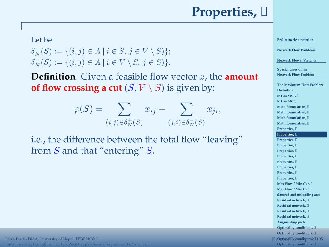
Preliminaries: notation
Network Flow Problems
Network Flows: Variants
Special cases of the
Network Flow Problem
The Maximum Flow Problem
Definition
MF as MCF, ➀
MF as MCF, ➁
Math formulation, ➀
Math formulation, ➁
Math formulation, ➂
Math formulation, ➃
Properties, ➀
Properties, ➁
Properties, ➂
Properties, ➃
Properties, ➃
Properties, ➃
Properties, ➃
Properties, ➃
Properties, ➃
Properties, ➄
Max Flow / Min Cut, ➀
Max Flow / Min Cut, ➁
Satured and unloading arcs
Residual network, ➀
Residual network, ➀
Residual network, ➁
Residual network, ➁
Augmenting path
Optimality conditions, ➀
Optimality conditions, ➁
Optimality conditions, ➁
Optimality conditions, ➁
A solution method:
Paola Festa - DMA, University of Napoli FEDERICO II
E-mail: [email protected] - Web: http://www.dma.unina.it/∼festaNetwork Flows - p. 42/105
Properties, ➁
Let be
δ+N (S) := {(i, j) ∈ A | i ∈ S, j ∈ V \ S)};
δ−N (S) := {(i, j) ∈ A | i ∈ V \ S, j ∈ S)}.
Definition. Given a feasible flow vector x, the amountof flow crossing a cut (S, V \ S) is given by:
ϕ(S) =∑
(i,j)∈δ+N(S)
xij −∑
(j,i)∈δ−
N(S)
xji,
i.e., the difference between the total flow “leaving”from S and that “entering” S.
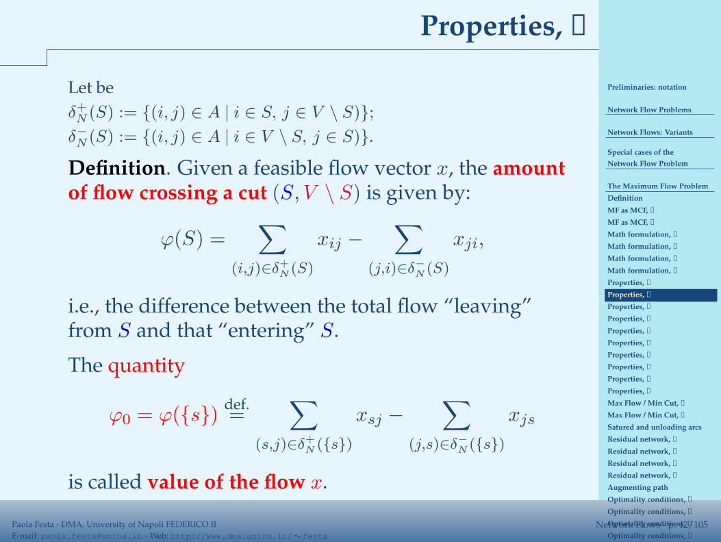
The quantity
ϕ0 = ϕ({s})def.=
∑
(s,j)∈δ+N ({s})
xsj −∑
(j,s)∈δ−
N({s})
xjs
is called value of the flow x.
Preliminaries: notation
Network Flow Problems
Network Flows: Variants
Special cases of the
Network Flow Problem
The Maximum Flow Problem
Definition
MF as MCF, ➀
MF as MCF, ➁
Math formulation, ➀
Math formulation, ➁
Math formulation, ➂
Math formulation, ➃
Properties, ➀
Properties, ➁
Properties, ➂
Properties, ➃
Properties, ➃
Properties, ➃
Properties, ➃
Properties, ➃
Properties, ➃
Properties, ➄
Max Flow / Min Cut, ➀
Max Flow / Min Cut, ➁
Satured and unloading arcs
Residual network, ➀
Residual network, ➀
Residual network, ➁
Residual network, ➁
Augmenting path
Optimality conditions, ➀
Optimality conditions, ➁
Optimality conditions, ➁
Optimality conditions, ➁
A solution method:
Paola Festa - DMA, University of Napoli FEDERICO II
E-mail: [email protected] - Web: http://www.dma.unina.it/∼festaNetwork Flows - p. 43/105
Properties, ➂
Definition. Given a cut (S, V \ S) in a network flowN = (V,A), the capacity of the cut (S, V \ S) is givenby:
K(S) =∑
(i,j)∈δ+N(S)
kij .
Note: K(S) does not take into account the capacities of
the arcs “entering” S, i.e. those belonging to δ−N (S).
Preliminaries: notation
Network Flow Problems
Network Flows: Variants
Special cases of the
Network Flow Problem
The Maximum Flow Problem
Definition
MF as MCF, ➀
MF as MCF, ➁
Math formulation, ➀
Math formulation, ➁
Math formulation, ➂
Math formulation, ➃
Properties, ➀
Properties, ➁
Properties, ➂
Properties, ➃
Properties, ➃
Properties, ➃
Properties, ➃
Properties, ➃
Properties, ➃
Properties, ➄
Max Flow / Min Cut, ➀
Max Flow / Min Cut, ➁
Satured and unloading arcs
Residual network, ➀
Residual network, ➀
Residual network, ➁
Residual network, ➁
Augmenting path
Optimality conditions, ➀
Optimality conditions, ➁
Optimality conditions, ➁
Optimality conditions, ➁
A solution method:
Paola Festa - DMA, University of Napoli FEDERICO II
E-mail: [email protected] - Web: http://www.dma.unina.it/∼festaNetwork Flows - p. 44/105
Properties, ➃
Theorem. Given a feasible flow vector x in a networkflow N = (V,A), for every cut (S, V \ S) in N it resultsthat
ϕ(S) = ϕ0 = ϕ({s}).
Note: the theorem claims that, for every cut (S, V \ S),the amount of flow that crosses it is always equal to
ϕ0, i.e. it is constant.
Preliminaries: notation
Network Flow Problems
Network Flows: Variants
Special cases of the
Network Flow Problem
The Maximum Flow Problem
Definition
MF as MCF, ➀
MF as MCF, ➁
Math formulation, ➀
Math formulation, ➁
Math formulation, ➂
Math formulation, ➃
Properties, ➀
Properties, ➁
Properties, ➂
Properties, ➃
Properties, ➃
Properties, ➃
Properties, ➃
Properties, ➃
Properties, ➃
Properties, ➄
Max Flow / Min Cut, ➀
Max Flow / Min Cut, ➁
Satured and unloading arcs
Residual network, ➀
Residual network, ➀
Residual network, ➁
Residual network, ➁
Augmenting path
Optimality conditions, ➀
Optimality conditions, ➁
Optimality conditions, ➁
Optimality conditions, ➁
A solution method:
Paola Festa - DMA, University of Napoli FEDERICO II
E-mail: [email protected] - Web: http://www.dma.unina.it/∼festaNetwork Flows - p. 45/105
Properties, ➃
Theorem. Given a feasible flow vector x in a networkflow N = (V,A), for every cut (S, V \ S) in N it resultsthat
ϕ(S) = ϕ0 = ϕ({s}).
Proof:from the flow conservation law applied to every nodei ∈ S \ {s}.
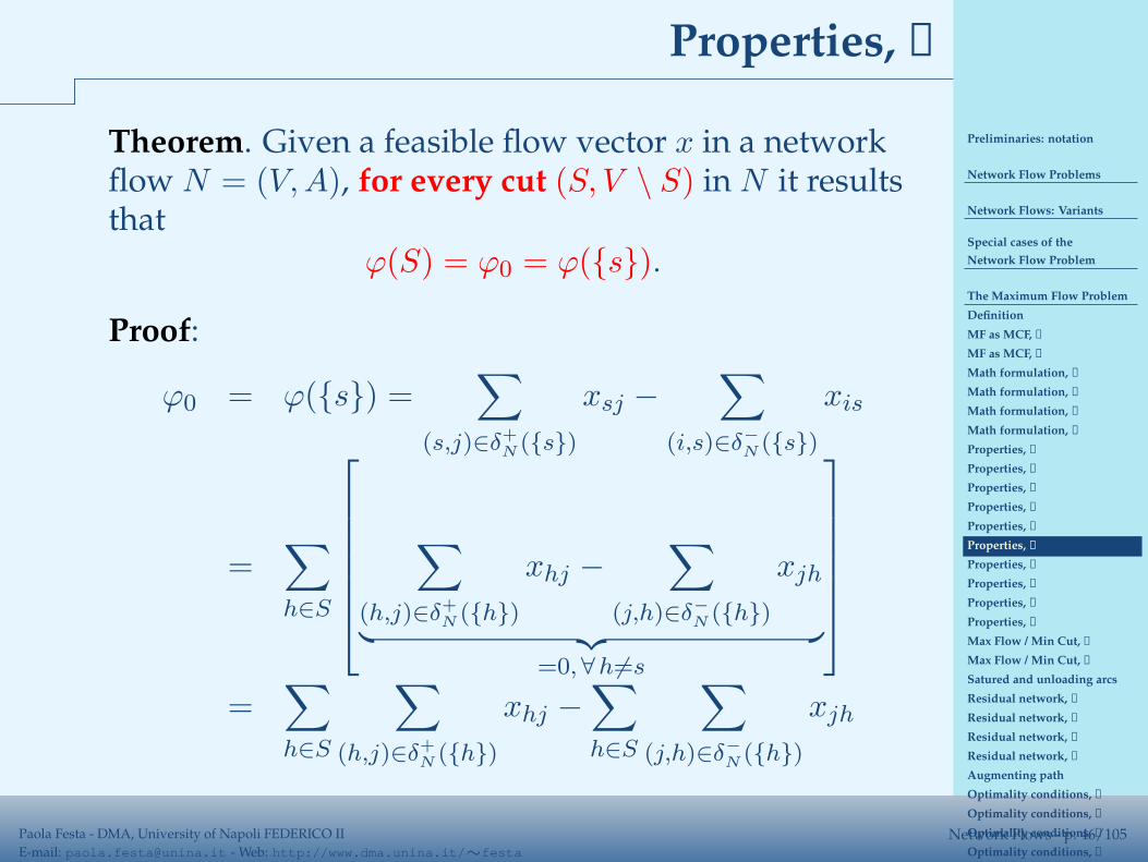
Preliminaries: notation
Network Flow Problems
Network Flows: Variants
Special cases of the
Network Flow Problem
The Maximum Flow Problem
Definition
MF as MCF, ➀
MF as MCF, ➁
Math formulation, ➀
Math formulation, ➁
Math formulation, ➂
Math formulation, ➃
Properties, ➀
Properties, ➁
Properties, ➂
Properties, ➃
Properties, ➃
Properties, ➃
Properties, ➃
Properties, ➃
Properties, ➃
Properties, ➄
Max Flow / Min Cut, ➀
Max Flow / Min Cut, ➁
Satured and unloading arcs
Residual network, ➀
Residual network, ➀
Residual network, ➁
Residual network, ➁
Augmenting path
Optimality conditions, ➀
Optimality conditions, ➁
Optimality conditions, ➁
Optimality conditions, ➁
A solution method:
Paola Festa - DMA, University of Napoli FEDERICO II
E-mail: [email protected] - Web: http://www.dma.unina.it/∼festaNetwork Flows - p. 46/105
Properties, ➃
Theorem. Given a feasible flow vector x in a networkflow N = (V,A), for every cut (S, V \ S) in N it resultsthat
ϕ(S) = ϕ0 = ϕ({s}).
Proof:
ϕ0 = ϕ({s}) =∑
(s,j)∈δ+N({s})
xsj −∑
(i,s)∈δ−
N({s})
xis
=∑
h∈S
∑
(h,j)∈δ+N ({h})
xhj −∑
(j,h)∈δ−
N ({h})
xjh
︸ ︷︷ ︸
=0,∀h6=s
=∑
h∈S
∑
(h,j)∈δ+N ({h})
xhj −∑
h∈S
∑
(j,h)∈δ−
N({h})
xjh

Preliminaries: notation
Network Flow Problems
Network Flows: Variants
Special cases of the
Network Flow Problem
The Maximum Flow Problem
Definition
MF as MCF, ➀
MF as MCF, ➁
Math formulation, ➀
Math formulation, ➁
Math formulation, ➂
Math formulation, ➃
Properties, ➀
Properties, ➁
Properties, ➂
Properties, ➃
Properties, ➃
Properties, ➃
Properties, ➃
Properties, ➃
Properties, ➃
Properties, ➄
Max Flow / Min Cut, ➀
Max Flow / Min Cut, ➁
Satured and unloading arcs
Residual network, ➀
Residual network, ➀
Residual network, ➁
Residual network, ➁
Augmenting path
Optimality conditions, ➀
Optimality conditions, ➁
Optimality conditions, ➁
Optimality conditions, ➁
A solution method:
Paola Festa - DMA, University of Napoli FEDERICO II
E-mail: [email protected] - Web: http://www.dma.unina.it/∼festaNetwork Flows - p. 47/105
Properties, ➃
Theorem. Given a feasible flow vector x in a networkflow N = (V,A), for every cut (S, V \ S) in N it resultsthat
ϕ(S) = ϕ0 = ϕ({s}).
Proof: Note that,∑
h∈S
∑
(h,j)∈δ+N
({h})
xhj =∑
h∈S
∑
j∈FS(h)
xhj =∑
(i,j)∈A(S)
xij +∑
(i,j)∈δ+N
(S)
xij
h
j
s
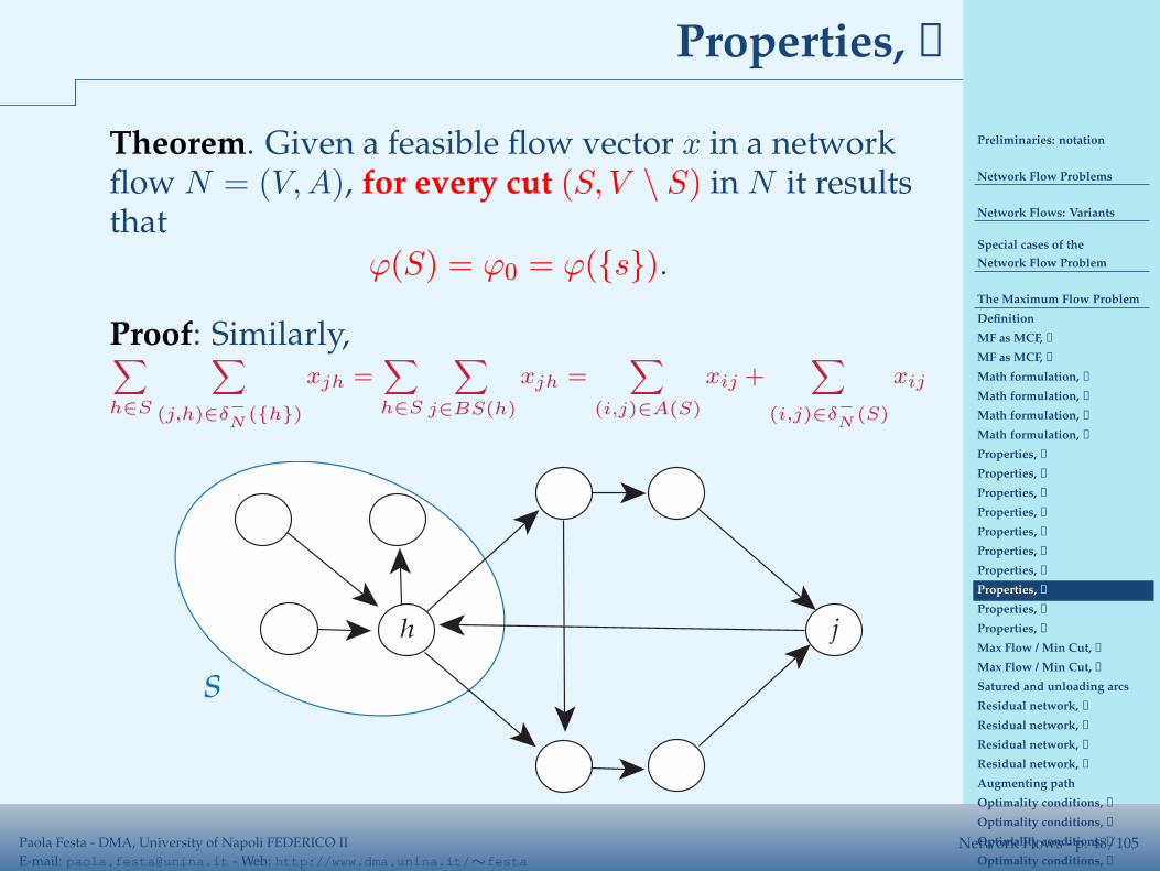
Preliminaries: notation
Network Flow Problems
Network Flows: Variants
Special cases of the
Network Flow Problem
The Maximum Flow Problem
Definition
MF as MCF, ➀
MF as MCF, ➁
Math formulation, ➀
Math formulation, ➁
Math formulation, ➂
Math formulation, ➃
Properties, ➀
Properties, ➁
Properties, ➂
Properties, ➃
Properties, ➃
Properties, ➃
Properties, ➃
Properties, ➃
Properties, ➃
Properties, ➄
Max Flow / Min Cut, ➀
Max Flow / Min Cut, ➁
Satured and unloading arcs
Residual network, ➀
Residual network, ➀
Residual network, ➁
Residual network, ➁
Augmenting path
Optimality conditions, ➀
Optimality conditions, ➁
Optimality conditions, ➁
Optimality conditions, ➁
A solution method:
Paola Festa - DMA, University of Napoli FEDERICO II
E-mail: [email protected] - Web: http://www.dma.unina.it/∼festaNetwork Flows - p. 48/105
Properties, ➃
Theorem. Given a feasible flow vector x in a networkflow N = (V,A), for every cut (S, V \ S) in N it resultsthat
ϕ(S) = ϕ0 = ϕ({s}).
Proof: Similarly,∑
h∈S
∑
(j,h)∈δ−
N({h})
xjh =∑
h∈S
∑
j∈BS(h)
xjh =∑
(i,j)∈A(S)
xij +∑
(i,j)∈δ−
N(S)
xij
h j
s
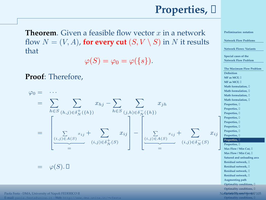
Preliminaries: notation
Network Flow Problems
Network Flows: Variants
Special cases of the
Network Flow Problem
The Maximum Flow Problem
Definition
MF as MCF, ➀
MF as MCF, ➁
Math formulation, ➀
Math formulation, ➁
Math formulation, ➂
Math formulation, ➃
Properties, ➀
Properties, ➁
Properties, ➂
Properties, ➃
Properties, ➃
Properties, ➃
Properties, ➃
Properties, ➃
Properties, ➃
Properties, ➄
Max Flow / Min Cut, ➀
Max Flow / Min Cut, ➁
Satured and unloading arcs
Residual network, ➀
Residual network, ➀
Residual network, ➁
Residual network, ➁
Augmenting path
Optimality conditions, ➀
Optimality conditions, ➁
Optimality conditions, ➁
Optimality conditions, ➁
A solution method:
Paola Festa - DMA, University of Napoli FEDERICO II
E-mail: [email protected] - Web: http://www.dma.unina.it/∼festaNetwork Flows - p. 49/105
Properties, ➃
Theorem. Given a feasible flow vector x in a networkflow N = (V,A), for every cut (S, V \ S) in N it resultsthat
ϕ(S) = ϕ0 = ϕ({s}).
Proof: Therefore,
ϕ0 = · · ·
=∑
h∈S
∑
(h,j)∈δ+N
({h})
xhj −∑
h∈S
∑
(j,h)∈δ−
N({h})
xjh
=
∑
(i,j)∈A(S)
xij
︸ ︷︷ ︸
=
+∑
(i,j)∈δ+N
(S)
xij
−
∑
(i,j)∈A(S)
xij
︸ ︷︷ ︸
=
+∑
(i,j)∈δ−
N(S)
xij
= ϕ(S).
Preliminaries: notation
Network Flow Problems
Network Flows: Variants
Special cases of the
Network Flow Problem
The Maximum Flow Problem
Definition
MF as MCF, ➀
MF as MCF, ➁
Math formulation, ➀
Math formulation, ➁
Math formulation, ➂
Math formulation, ➃
Properties, ➀
Properties, ➁
Properties, ➂
Properties, ➃
Properties, ➃
Properties, ➃
Properties, ➃
Properties, ➃
Properties, ➃
Properties, ➄
Max Flow / Min Cut, ➀
Max Flow / Min Cut, ➁
Satured and unloading arcs
Residual network, ➀
Residual network, ➀
Residual network, ➁
Residual network, ➁
Augmenting path
Optimality conditions, ➀
Optimality conditions, ➁
Optimality conditions, ➁
Optimality conditions, ➁
A solution method:
Paola Festa - DMA, University of Napoli FEDERICO II
E-mail: [email protected] - Web: http://www.dma.unina.it/∼festaNetwork Flows - p. 50/105
Properties, ➄
Theorem. For every feasible flow x in a network flowN = (V,A) and for every cut (S, V \ S) in N , it resultsthat
ϕ(S) ≤ K(S).
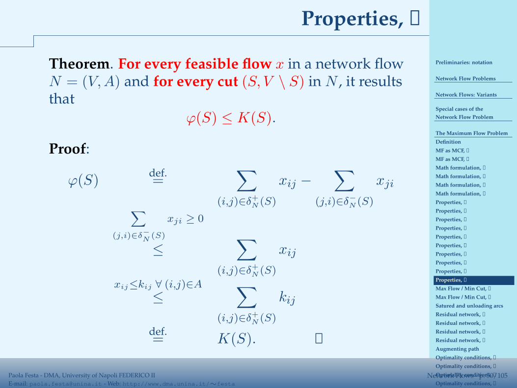
Proof:
ϕ(S)def.=
∑
(i,j)∈δ+N (S)
xij −∑
(j,i)∈δ−
N(S)
xji
∑
(j,i)∈δ−
N(S)
xji ≥ 0
≤∑
(i,j)∈δ+N (S)
xij
xij≤kij ∀ (i,j)∈A
≤∑
(i,j)∈δ+N (S)
kij
def.= K(S).

Preliminaries: notation
Network Flow Problems
Network Flows: Variants
Special cases of the
Network Flow Problem
The Maximum Flow Problem
Definition
MF as MCF, ➀
MF as MCF, ➁
Math formulation, ➀
Math formulation, ➁
Math formulation, ➂
Math formulation, ➃
Properties, ➀
Properties, ➁
Properties, ➂
Properties, ➃
Properties, ➃
Properties, ➃
Properties, ➃
Properties, ➃
Properties, ➃
Properties, ➄
Max Flow / Min Cut, ➀
Max Flow / Min Cut, ➁
Satured and unloading arcs
Residual network, ➀
Residual network, ➀
Residual network, ➁
Residual network, ➁
Augmenting path
Optimality conditions, ➀
Optimality conditions, ➁
Optimality conditions, ➁
Optimality conditions, ➁
A solution method:
Paola Festa - DMA, University of Napoli FEDERICO II
E-mail: [email protected] - Web: http://www.dma.unina.it/∼festaNetwork Flows - p. 51/105
Max Flow / Min Cut, ➀
Theorem [Maximum Flow / Minimum Cut].
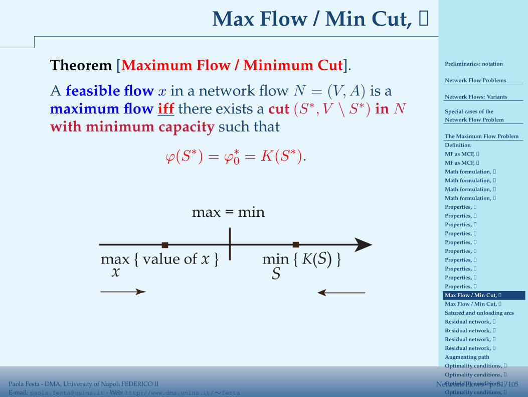
A feasible flow x in a network flow N = (V,A) is amaximum flow iff there exists a cut (S∗, V \ S∗) in N
with minimum capacity such that
ϕ(S∗) = ϕ∗0 = K(S∗).
max = min
max { value of x } min { K(S) }x S
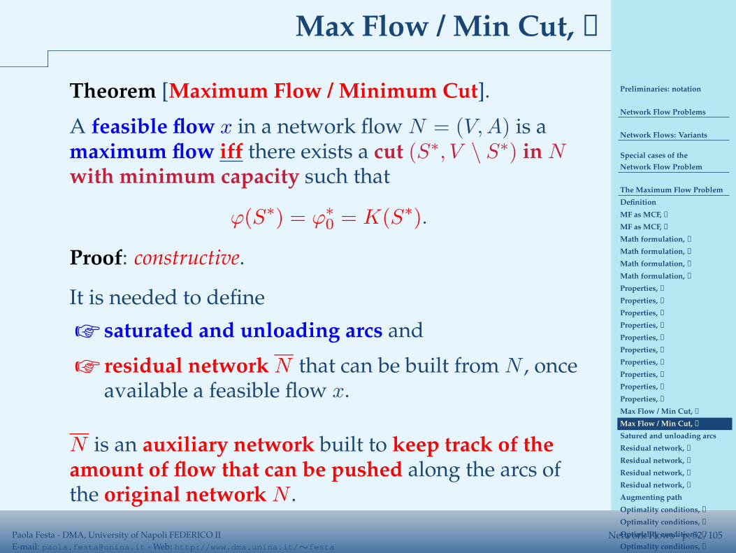
Preliminaries: notation
Network Flow Problems
Network Flows: Variants
Special cases of the
Network Flow Problem
The Maximum Flow Problem
Definition
MF as MCF, ➀
MF as MCF, ➁
Math formulation, ➀
Math formulation, ➁
Math formulation, ➂
Math formulation, ➃
Properties, ➀
Properties, ➁
Properties, ➂
Properties, ➃
Properties, ➃
Properties, ➃
Properties, ➃
Properties, ➃
Properties, ➃
Properties, ➄
Max Flow / Min Cut, ➀
Max Flow / Min Cut, ➁
Satured and unloading arcs
Residual network, ➀
Residual network, ➀
Residual network, ➁
Residual network, ➁
Augmenting path
Optimality conditions, ➀
Optimality conditions, ➁
Optimality conditions, ➁
Optimality conditions, ➁
A solution method:
Paola Festa - DMA, University of Napoli FEDERICO II
E-mail: [email protected] - Web: http://www.dma.unina.it/∼festaNetwork Flows - p. 52/105
Max Flow / Min Cut, ➁
Theorem [Maximum Flow / Minimum Cut].
A feasible flow x in a network flow N = (V,A) is amaximum flow iff there exists a cut (S∗, V \ S∗) in N
with minimum capacity such that
ϕ(S∗) = ϕ∗0 = K(S∗).
Proof: constructive.
It is needed to define
☞ saturated and unloading arcs and
☞ residual network N that can be built from N , onceavailable a feasible flow x.
N is an auxiliary network built to keep track of theamount of flow that can be pushed along the arcs ofthe original network N .
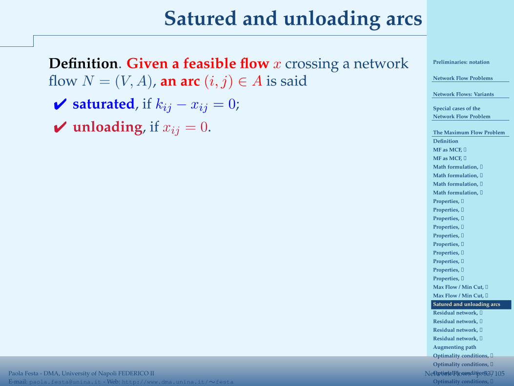
Preliminaries: notation
Network Flow Problems
Network Flows: Variants
Special cases of the
Network Flow Problem
The Maximum Flow Problem
Definition
MF as MCF, ➀
MF as MCF, ➁
Math formulation, ➀
Math formulation, ➁
Math formulation, ➂
Math formulation, ➃
Properties, ➀
Properties, ➁
Properties, ➂
Properties, ➃
Properties, ➃
Properties, ➃
Properties, ➃
Properties, ➃
Properties, ➃
Properties, ➄
Max Flow / Min Cut, ➀
Max Flow / Min Cut, ➁
Satured and unloading arcs
Residual network, ➀
Residual network, ➀
Residual network, ➁
Residual network, ➁
Augmenting path
Optimality conditions, ➀
Optimality conditions, ➁
Optimality conditions, ➁
Optimality conditions, ➁
A solution method:
Paola Festa - DMA, University of Napoli FEDERICO II
E-mail: [email protected] - Web: http://www.dma.unina.it/∼festaNetwork Flows - p. 53/105
Satured and unloading arcs
Definition. Given a feasible flow x crossing a networkflow N = (V,A), an arc (i, j) ∈ A is said
✔ saturated, if kij − xij = 0;
✔ unloading, if xij = 0.
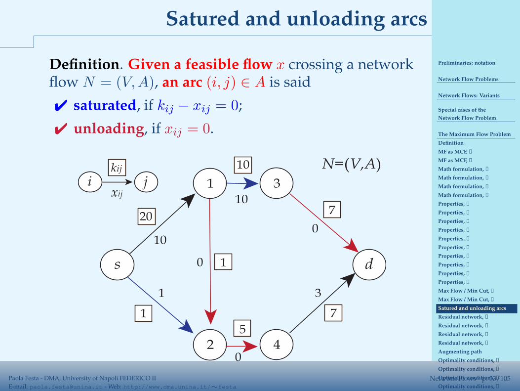
xij
s
1
d
2
1
ikij
j 3
4
10 N=(V,A)
10
0
1
20
10
1
5
0
7
7
0
3
Preliminaries: notation
Network Flow Problems
Network Flows: Variants
Special cases of the
Network Flow Problem
The Maximum Flow Problem
Definition
MF as MCF, ➀
MF as MCF, ➁
Math formulation, ➀
Math formulation, ➁
Math formulation, ➂
Math formulation, ➃
Properties, ➀
Properties, ➁
Properties, ➂
Properties, ➃
Properties, ➃
Properties, ➃
Properties, ➃
Properties, ➃
Properties, ➃
Properties, ➄
Max Flow / Min Cut, ➀
Max Flow / Min Cut, ➁
Satured and unloading arcs
Residual network, ➀
Residual network, ➀
Residual network, ➁
Residual network, ➁
Augmenting path
Optimality conditions, ➀
Optimality conditions, ➁
Optimality conditions, ➁
Optimality conditions, ➁
A solution method:
Paola Festa - DMA, University of Napoli FEDERICO II
E-mail: [email protected] - Web: http://www.dma.unina.it/∼festaNetwork Flows - p. 54/105
Residual network, ➀
Definition. Given a feasible flow x crossing a network
flow N = (V,A), the residual network N = (V,A)associated with N is built performing the following 2operations:
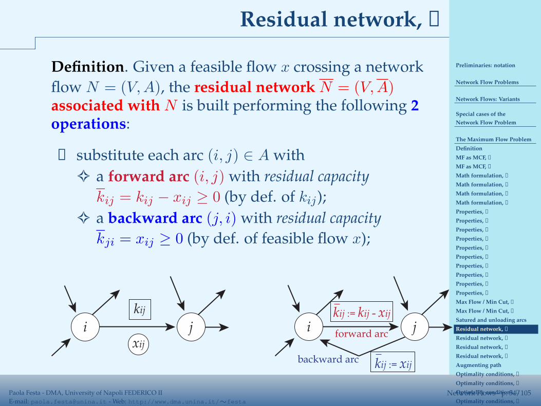
① substitute each arc (i, j) ∈ A with
✧ a forward arc (i, j) with residual capacity
kij = kij − xij ≥ 0 (by def. of kij);
✧ a backward arc (j, i) with residual capacity
kji = xij ≥ 0 (by def. of feasible flow x);
i j
kij
xij
i jkij := kij - xij
forward arc
backward arc kij := xij
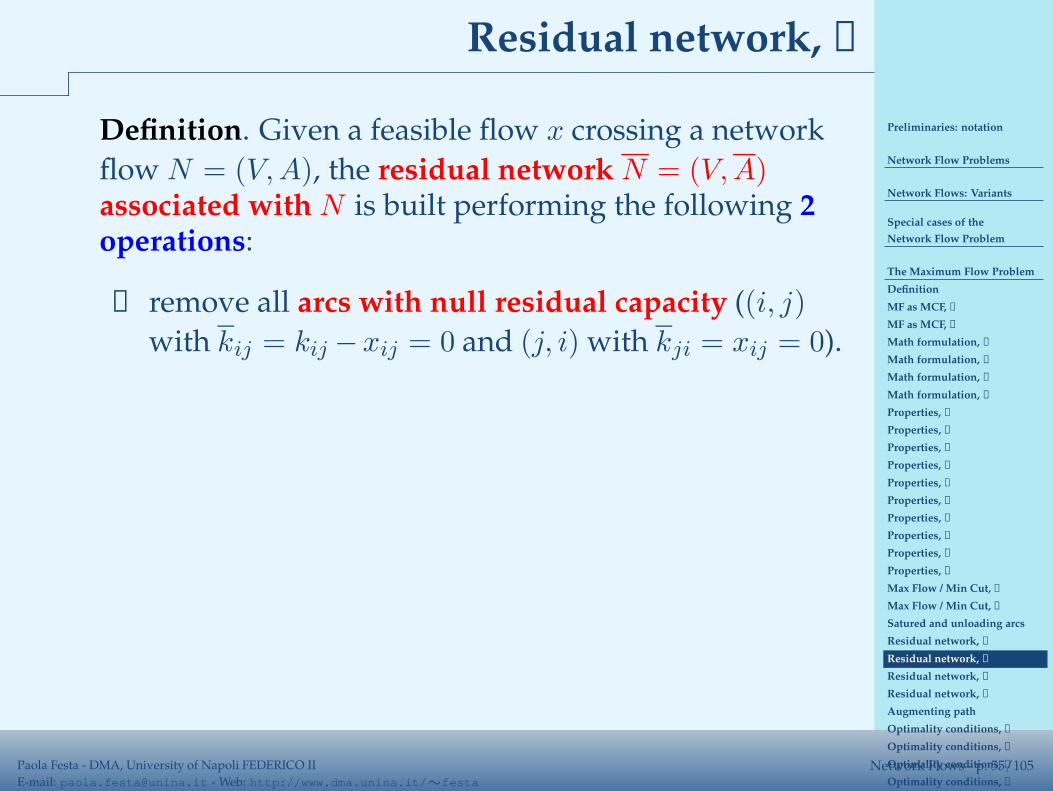
Preliminaries: notation
Network Flow Problems
Network Flows: Variants
Special cases of the
Network Flow Problem
The Maximum Flow Problem
Definition
MF as MCF, ➀
MF as MCF, ➁
Math formulation, ➀
Math formulation, ➁
Math formulation, ➂
Math formulation, ➃
Properties, ➀
Properties, ➁
Properties, ➂
Properties, ➃
Properties, ➃
Properties, ➃
Properties, ➃
Properties, ➃
Properties, ➃
Properties, ➄
Max Flow / Min Cut, ➀
Max Flow / Min Cut, ➁
Satured and unloading arcs
Residual network, ➀
Residual network, ➀
Residual network, ➁
Residual network, ➁
Augmenting path
Optimality conditions, ➀
Optimality conditions, ➁
Optimality conditions, ➁
Optimality conditions, ➁
A solution method:
Paola Festa - DMA, University of Napoli FEDERICO II
E-mail: [email protected] - Web: http://www.dma.unina.it/∼festaNetwork Flows - p. 55/105
Residual network, ➀
Definition. Given a feasible flow x crossing a network
flow N = (V,A), the residual network N = (V,A)associated with N is built performing the following 2operations:
② remove all arcs with null residual capacity ((i, j)
with kij = kij −xij = 0 and (j, i) with kji = xij = 0).
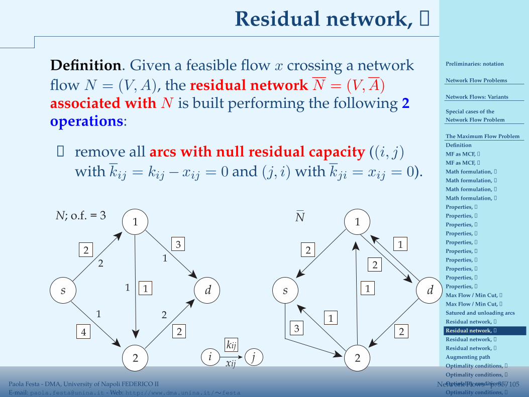
s
1
d
2
1
21
2
2
4
1 1
3
2
s
1
d
2
2
3
1
1
2
1
N; o.f. = 3 N
2
ikij
jxij
Preliminaries: notation
Network Flow Problems
Network Flows: Variants
Special cases of the
Network Flow Problem
The Maximum Flow Problem
Definition
MF as MCF, ➀
MF as MCF, ➁
Math formulation, ➀
Math formulation, ➁
Math formulation, ➂
Math formulation, ➃
Properties, ➀
Properties, ➁
Properties, ➂
Properties, ➃
Properties, ➃
Properties, ➃
Properties, ➃
Properties, ➃
Properties, ➃
Properties, ➄
Max Flow / Min Cut, ➀
Max Flow / Min Cut, ➁
Satured and unloading arcs
Residual network, ➀
Residual network, ➀
Residual network, ➁
Residual network, ➁
Augmenting path
Optimality conditions, ➀
Optimality conditions, ➁
Optimality conditions, ➁
Optimality conditions, ➁
A solution method:
Paola Festa - DMA, University of Napoli FEDERICO II
E-mail: [email protected] - Web: http://www.dma.unina.it/∼festaNetwork Flows - p. 56/105
Residual network, ➁
The residual network N allows to find a flow x froms ∈ V to d ∈ V higher than x,
✓ increasing the flow along non saturated arcs
(i.e., those arcs (i, j) with kij = kij − xij 6= 0) and
✓ decreasing it along non unloading arcs
(i.e., those arcs (j, i) with kji = xij 6= 0).
If ∃ P from s to d in N =⇒ ∃ in N x higher than x!
P from s to d is said augmenting path and in N itcorresponds to a sequence
✍ of forward arcs along which to increase thecurrent flow and
✍ of backward arcs along which to decrease thecurrent flow.
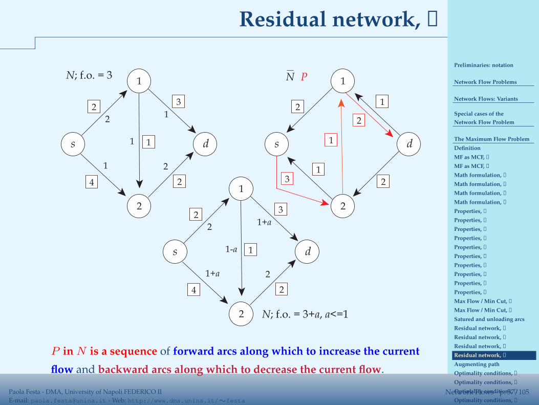
Preliminaries: notation
Network Flow Problems
Network Flows: Variants
Special cases of the
Network Flow Problem
The Maximum Flow Problem
Definition
MF as MCF, ➀
MF as MCF, ➁
Math formulation, ➀
Math formulation, ➁
Math formulation, ➂
Math formulation, ➃
Properties, ➀
Properties, ➁
Properties, ➂
Properties, ➃
Properties, ➃
Properties, ➃
Properties, ➃
Properties, ➃
Properties, ➃
Properties, ➄
Max Flow / Min Cut, ➀
Max Flow / Min Cut, ➁
Satured and unloading arcs
Residual network, ➀
Residual network, ➀
Residual network, ➁
Residual network, ➁
Augmenting path
Optimality conditions, ➀
Optimality conditions, ➁
Optimality conditions, ➁
Optimality conditions, ➁
A solution method:
Paola Festa - DMA, University of Napoli FEDERICO II
E-mail: [email protected] - Web: http://www.dma.unina.it/∼festaNetwork Flows - p. 57/105
Residual network, ➁
s
1
d
2
1
21
2
2
4
1 1
3
2
s
1
d
2
2
3
1
2
1
1
N; f.o. = 3 N P
2
s
1
d
2
1+a
21+a
2
2
4
1-a 1
3
2
N; f.o. = 3+a, a<=1
P in N is a sequence of forward arcs along which to increase the current
flow and backward arcs along which to decrease the current flow.
Preliminaries: notation
Network Flow Problems
Network Flows: Variants
Special cases of the
Network Flow Problem
The Maximum Flow Problem
Definition
MF as MCF, ➀
MF as MCF, ➁
Math formulation, ➀
Math formulation, ➁
Math formulation, ➂
Math formulation, ➃
Properties, ➀
Properties, ➁
Properties, ➂
Properties, ➃
Properties, ➃
Properties, ➃
Properties, ➃
Properties, ➃
Properties, ➃
Properties, ➄
Max Flow / Min Cut, ➀
Max Flow / Min Cut, ➁
Satured and unloading arcs
Residual network, ➀
Residual network, ➀
Residual network, ➁
Residual network, ➁
Augmenting path
Optimality conditions, ➀
Optimality conditions, ➁
Optimality conditions, ➁
Optimality conditions, ➁
A solution method:
Paola Festa - DMA, University of Napoli FEDERICO II
E-mail: [email protected] - Web: http://www.dma.unina.it/∼festaNetwork Flows - p. 58/105
Augmenting path
Definition. Given a feasible flow x in a network flowN = (V,A), an augmenting path is a path P from thesource s to the sink d in N s.t., denoting by
❒ F the set of forward arcs in P and
❒ B the set of backward arcs in P ,
it results that
❍ xij < kij , ∀ (i, j) ∈ F =⇒it is possible to increase the current flow along (i, j)!
❍ xij > 0, ∀ (i, j) ∈ B=⇒it is possible to decrease the current flow along(i, j)!
Preliminaries: notation
Network Flow Problems
Network Flows: Variants
Special cases of the
Network Flow Problem
The Maximum Flow Problem
Definition
MF as MCF, ➀
MF as MCF, ➁
Math formulation, ➀
Math formulation, ➁
Math formulation, ➂
Math formulation, ➃
Properties, ➀
Properties, ➁
Properties, ➂
Properties, ➃
Properties, ➃
Properties, ➃
Properties, ➃
Properties, ➃
Properties, ➃
Properties, ➄
Max Flow / Min Cut, ➀
Max Flow / Min Cut, ➁
Satured and unloading arcs
Residual network, ➀
Residual network, ➀
Residual network, ➁
Residual network, ➁
Augmenting path
Optimality conditions, ➀
Optimality conditions, ➁
Optimality conditions, ➁
Optimality conditions, ➁
A solution method:
Paola Festa - DMA, University of Napoli FEDERICO II
E-mail: [email protected] - Web: http://www.dma.unina.it/∼festaNetwork Flows - p. 59/105
Optimality conditions, ➀
Theorem. A feasible flow x in a network flowN = (V,A) is optimal for MF iff node d can not be
reached from node s in the residual network N .
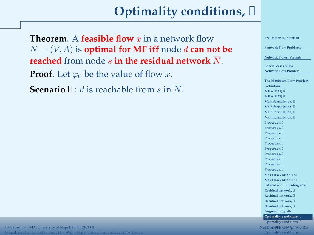
Proof. Let ϕ0 be the value of flow x.
Scenario ①: d is reachable from s in N .
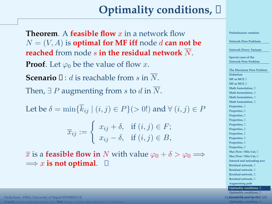
Then, ∃ P augmenting from s to d in N .
Let be δ = min{kij | (i, j) ∈ P}(> 0!) and ∀ (i, j) ∈ P
xij :=
{
xij + δ, if (i, j) ∈ F ;
xij − δ, if (i, j) ∈ B,
x is a feasible flow in N with value ϕ0 + δ > ϕ0 =⇒=⇒ x is not optimal.
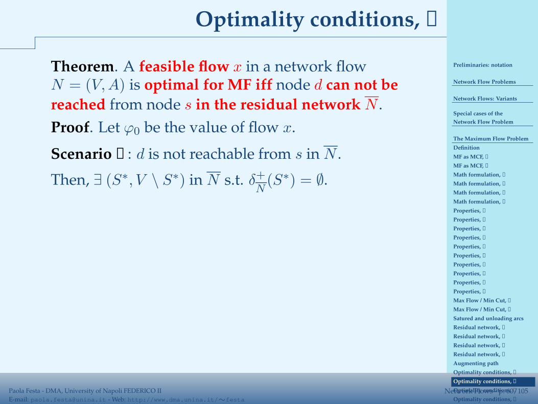
Preliminaries: notation
Network Flow Problems
Network Flows: Variants
Special cases of the
Network Flow Problem
The Maximum Flow Problem
Definition
MF as MCF, ➀
MF as MCF, ➁
Math formulation, ➀
Math formulation, ➁
Math formulation, ➂
Math formulation, ➃
Properties, ➀
Properties, ➁
Properties, ➂
Properties, ➃
Properties, ➃
Properties, ➃
Properties, ➃
Properties, ➃
Properties, ➃
Properties, ➄
Max Flow / Min Cut, ➀
Max Flow / Min Cut, ➁
Satured and unloading arcs
Residual network, ➀
Residual network, ➀
Residual network, ➁
Residual network, ➁
Augmenting path
Optimality conditions, ➀
Optimality conditions, ➁
Optimality conditions, ➁
Optimality conditions, ➁
A solution method:
Paola Festa - DMA, University of Napoli FEDERICO II
E-mail: [email protected] - Web: http://www.dma.unina.it/∼festaNetwork Flows - p. 60/105
Optimality conditions, ➁
Theorem. A feasible flow x in a network flowN = (V,A) is optimal for MF iff node d can not be
reached from node s in the residual network N .
Proof. Let ϕ0 be the value of flow x.
Scenario ②: d is not reachable from s in N .
Then, ∃ (S∗, V \ S∗) in N s.t. δ+N
(S∗) = ∅.
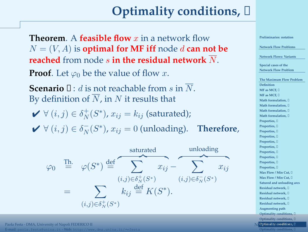
Preliminaries: notation
Network Flow Problems
Network Flows: Variants
Special cases of the
Network Flow Problem
The Maximum Flow Problem
Definition
MF as MCF, ➀
MF as MCF, ➁
Math formulation, ➀
Math formulation, ➁
Math formulation, ➂
Math formulation, ➃
Properties, ➀
Properties, ➁
Properties, ➂
Properties, ➃
Properties, ➃
Properties, ➃
Properties, ➃
Properties, ➃
Properties, ➃
Properties, ➄
Max Flow / Min Cut, ➀
Max Flow / Min Cut, ➁
Satured and unloading arcs
Residual network, ➀
Residual network, ➀
Residual network, ➁
Residual network, ➁
Augmenting path
Optimality conditions, ➀
Optimality conditions, ➁
Optimality conditions, ➁
Optimality conditions, ➁
A solution method:
Paola Festa - DMA, University of Napoli FEDERICO II
E-mail: [email protected] - Web: http://www.dma.unina.it/∼festaNetwork Flows - p. 61/105
Optimality conditions, ➁
Theorem. A feasible flow x in a network flowN = (V,A) is optimal for MF iff node d can not be
reached from node s in the residual network N .
Proof. Let ϕ0 be the value of flow x.
Scenario ②: d is not reachable from s in N .By definition of N , in N it results that
✔ ∀ (i, j) ∈ δ+N (S∗), xij = kij (saturated);
✔ ∀ (i, j) ∈ δ−N (S∗), xij = 0 (unloading). Therefore,
ϕ0Th.= ϕ(S∗)
def=
saturated︷ ︸︸ ︷
∑
(i,j)∈δ+N (S∗)
xij −
unloading︷ ︸︸ ︷
∑
(i,j)∈δ−
N (S∗)
xij
=∑
(i,j)∈δ+N (S∗)
kijdef= K(S∗).
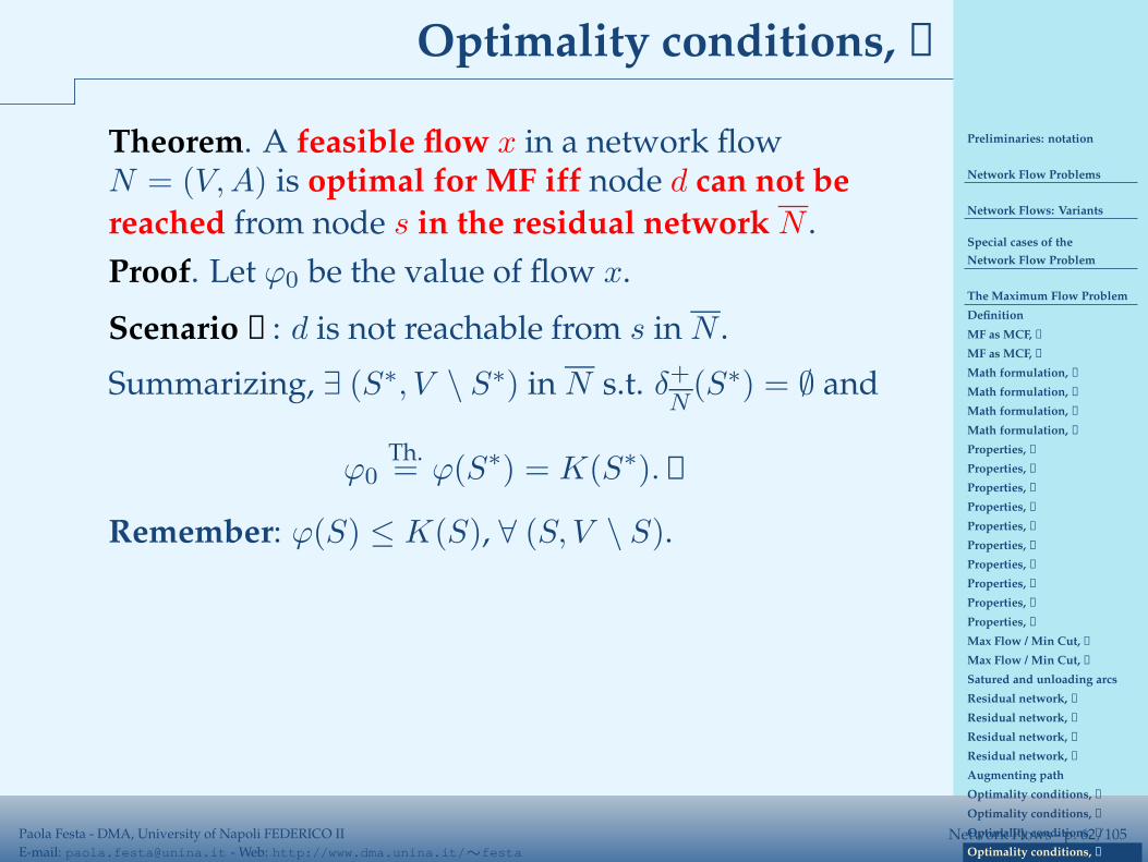
Preliminaries: notation
Network Flow Problems
Network Flows: Variants
Special cases of the
Network Flow Problem
The Maximum Flow Problem
Definition
MF as MCF, ➀
MF as MCF, ➁
Math formulation, ➀
Math formulation, ➁
Math formulation, ➂
Math formulation, ➃
Properties, ➀
Properties, ➁
Properties, ➂
Properties, ➃
Properties, ➃
Properties, ➃
Properties, ➃
Properties, ➃
Properties, ➃
Properties, ➄
Max Flow / Min Cut, ➀
Max Flow / Min Cut, ➁
Satured and unloading arcs
Residual network, ➀
Residual network, ➀
Residual network, ➁
Residual network, ➁
Augmenting path
Optimality conditions, ➀
Optimality conditions, ➁
Optimality conditions, ➁
Optimality conditions, ➁
A solution method:
Paola Festa - DMA, University of Napoli FEDERICO II
E-mail: [email protected] - Web: http://www.dma.unina.it/∼festaNetwork Flows - p. 62/105
Optimality conditions, ➁
Theorem. A feasible flow x in a network flowN = (V,A) is optimal for MF iff node d can not be
reached from node s in the residual network N .
Proof. Let ϕ0 be the value of flow x.
Scenario ②: d is not reachable from s in N .
Summarizing, ∃ (S∗, V \ S∗) in N s.t. δ+N
(S∗) = ∅ and
ϕ0Th.= ϕ(S∗) = K(S∗).
Remember: ϕ(S) ≤ K(S), ∀ (S, V \ S).
Preliminaries: notation
Network Flow Problems
Network Flows: Variants
Special cases of the
Network Flow Problem
The Maximum Flow Problem
A solution method:
the Ford-Fulkerson algorithm
Ford-Fulkerson algorithm, ➀
Ford-Fulkerson algorithm, ➁
Ford-Fulkerson algorithm, ➂
Ford-Fulkerson algorithm, ➂
Ford-Fulkerson algorithm, ➂
Ford-Fulkerson algorithm, ➂
Ford-Fulkerson algorithm, ➃
Ford-Fulkerson algorithm, ➃
Ford-Fulkerson algorithm, ➃
Ford-Fulkerson: complexity, ➀
Ford-Fulkerson: complexity, ➁
Ford-Fulkerson: complexity, ➂
A simpler (not more efficient)
implementation
of Ford-Fulkerson algorithm
Ford-Fulkerson algorithm:
an exercise
Paola Festa - DMA, University of Napoli FEDERICO II
E-mail: [email protected] - Web: http://www.dma.unina.it/∼festaNetwork Flows - p. 63/105
A solution method:the Ford-Fulkerson algorithm
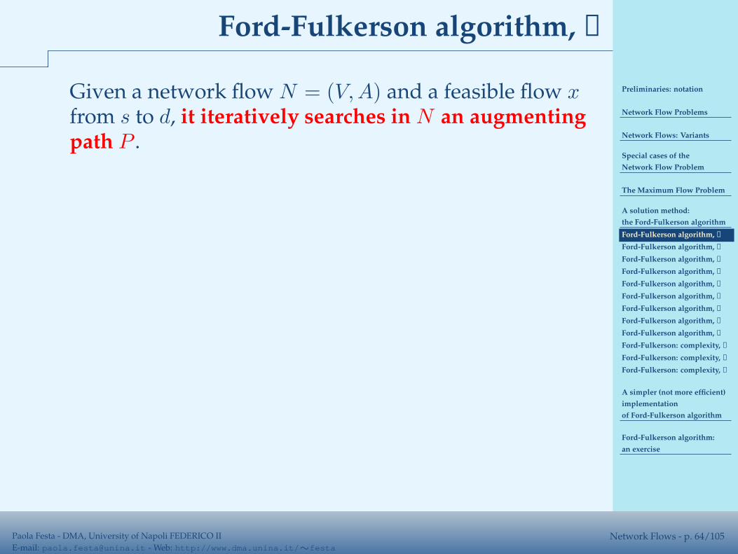
Preliminaries: notation
Network Flow Problems
Network Flows: Variants
Special cases of the
Network Flow Problem
The Maximum Flow Problem
A solution method:
the Ford-Fulkerson algorithm
Ford-Fulkerson algorithm, ➀
Ford-Fulkerson algorithm, ➁
Ford-Fulkerson algorithm, ➂
Ford-Fulkerson algorithm, ➂
Ford-Fulkerson algorithm, ➂
Ford-Fulkerson algorithm, ➂
Ford-Fulkerson algorithm, ➃
Ford-Fulkerson algorithm, ➃
Ford-Fulkerson algorithm, ➃
Ford-Fulkerson: complexity, ➀
Ford-Fulkerson: complexity, ➁
Ford-Fulkerson: complexity, ➂
A simpler (not more efficient)
implementation
of Ford-Fulkerson algorithm
Ford-Fulkerson algorithm:
an exercise
Paola Festa - DMA, University of Napoli FEDERICO II
E-mail: [email protected] - Web: http://www.dma.unina.it/∼festaNetwork Flows - p. 64/105
Ford-Fulkerson algorithm, ➀
Given a network flow N = (V,A) and a feasible flow x
from s to d, it iteratively searches in N an augmentingpath P .
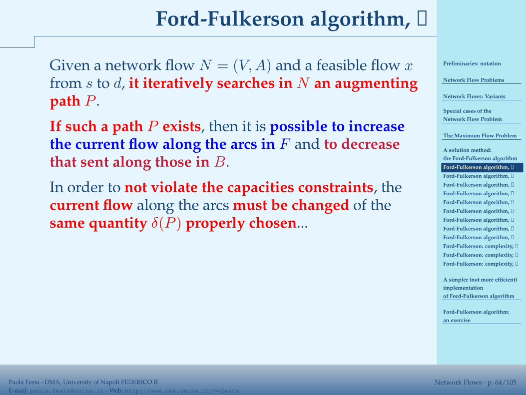
If such a path P exists, then it is possible to increasethe current flow along the arcs in F and to decreasethat sent along those in B.
In order to not violate the capacities constraints, thecurrent flow along the arcs must be changed of thesame quantity δ(P ) properly chosen...
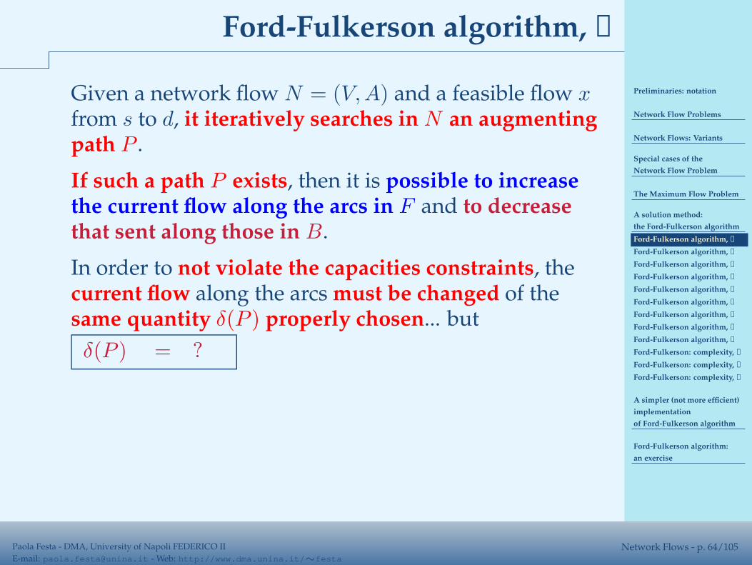
Preliminaries: notation
Network Flow Problems
Network Flows: Variants
Special cases of the
Network Flow Problem
The Maximum Flow Problem
A solution method:
the Ford-Fulkerson algorithm
Ford-Fulkerson algorithm, ➀
Ford-Fulkerson algorithm, ➁
Ford-Fulkerson algorithm, ➂
Ford-Fulkerson algorithm, ➂
Ford-Fulkerson algorithm, ➂
Ford-Fulkerson algorithm, ➂
Ford-Fulkerson algorithm, ➃
Ford-Fulkerson algorithm, ➃
Ford-Fulkerson algorithm, ➃
Ford-Fulkerson: complexity, ➀
Ford-Fulkerson: complexity, ➁
Ford-Fulkerson: complexity, ➂
A simpler (not more efficient)
implementation
of Ford-Fulkerson algorithm
Ford-Fulkerson algorithm:
an exercise
Paola Festa - DMA, University of Napoli FEDERICO II
E-mail: [email protected] - Web: http://www.dma.unina.it/∼festaNetwork Flows - p. 64/105
Ford-Fulkerson algorithm, ➀
Given a network flow N = (V,A) and a feasible flow x
from s to d, it iteratively searches in N an augmentingpath P .
If such a path P exists, then it is possible to increasethe current flow along the arcs in F and to decreasethat sent along those in B.
In order to not violate the capacities constraints, thecurrent flow along the arcs must be changed of thesame quantity δ(P ) properly chosen... but
δ(P ) = ?
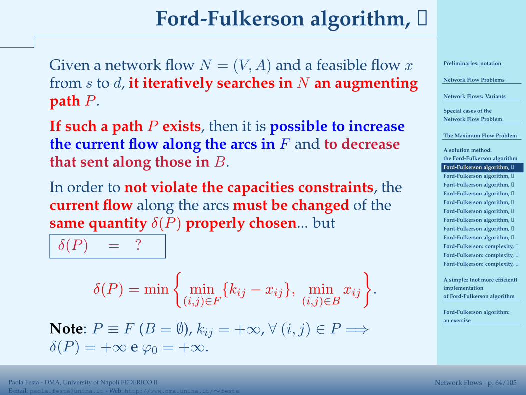
δ(P ) = min
{
min(i,j)∈F
{kij − xij}, min(i,j)∈B
xij
}
.
Note: P ≡ F (B = ∅), kij = +∞, ∀ (i, j) ∈ P =⇒δ(P ) = +∞ e ϕ0 = +∞.
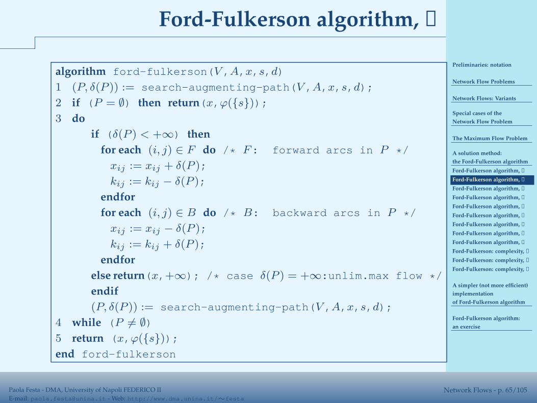
Preliminaries: notation
Network Flow Problems
Network Flows: Variants
Special cases of the
Network Flow Problem
The Maximum Flow Problem
A solution method:
the Ford-Fulkerson algorithm
Ford-Fulkerson algorithm, ➀
Ford-Fulkerson algorithm, ➁
Ford-Fulkerson algorithm, ➂
Ford-Fulkerson algorithm, ➂
Ford-Fulkerson algorithm, ➂
Ford-Fulkerson algorithm, ➂
Ford-Fulkerson algorithm, ➃
Ford-Fulkerson algorithm, ➃
Ford-Fulkerson algorithm, ➃
Ford-Fulkerson: complexity, ➀
Ford-Fulkerson: complexity, ➁
Ford-Fulkerson: complexity, ➂
A simpler (not more efficient)
implementation
of Ford-Fulkerson algorithm
Ford-Fulkerson algorithm:
an exercise
Paola Festa - DMA, University of Napoli FEDERICO II
E-mail: [email protected] - Web: http://www.dma.unina.it/∼festaNetwork Flows - p. 65/105
Ford-Fulkerson algorithm, ➁
algorithm ford-fulkerson(V ,A,x,s,d)
1 (P, δ(P )) := search-augmenting-path(V ,A,x,s,d);
2 if (P = ∅) then return(x,ϕ({s}));
3 do
if (δ(P ) < +∞) then
for each (i, j) ∈ F do /* F: forward arcs in P */
xij := xij + δ(P );
kij := kij − δ(P );
endfor
for each (i, j) ∈ B do /* B: backward arcs in P */
xij := xij − δ(P );
kij := kij + δ(P );
endfor
else return(x,+∞); /* case δ(P ) = +∞:unlim.max flow */
endif
(P, δ(P )) := search-augmenting-path(V ,A,x,s,d);
4 while (P 6= ∅)
5 return (x,ϕ({s}));
end ford-fulkerson
Preliminaries: notation
Network Flow Problems
Network Flows: Variants
Special cases of the
Network Flow Problem
The Maximum Flow Problem
A solution method:
the Ford-Fulkerson algorithm
Ford-Fulkerson algorithm, ➀
Ford-Fulkerson algorithm, ➁
Ford-Fulkerson algorithm, ➂
Ford-Fulkerson algorithm, ➂
Ford-Fulkerson algorithm, ➂
Ford-Fulkerson algorithm, ➂
Ford-Fulkerson algorithm, ➃
Ford-Fulkerson algorithm, ➃
Ford-Fulkerson algorithm, ➃
Ford-Fulkerson: complexity, ➀
Ford-Fulkerson: complexity, ➁
Ford-Fulkerson: complexity, ➂
A simpler (not more efficient)
implementation
of Ford-Fulkerson algorithm
Ford-Fulkerson algorithm:
an exercise
Paola Festa - DMA, University of Napoli FEDERICO II
E-mail: [email protected] - Web: http://www.dma.unina.it/∼festaNetwork Flows - p. 66/105
Ford-Fulkerson algorithm, ➂
Function search-augmenting-path.
Input: V , A, x, s, and d.
Output: P , δ(P ).
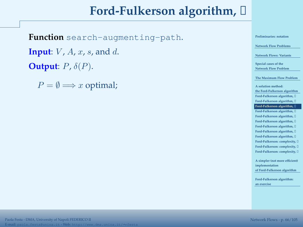
P = ∅ =⇒ x optimal;
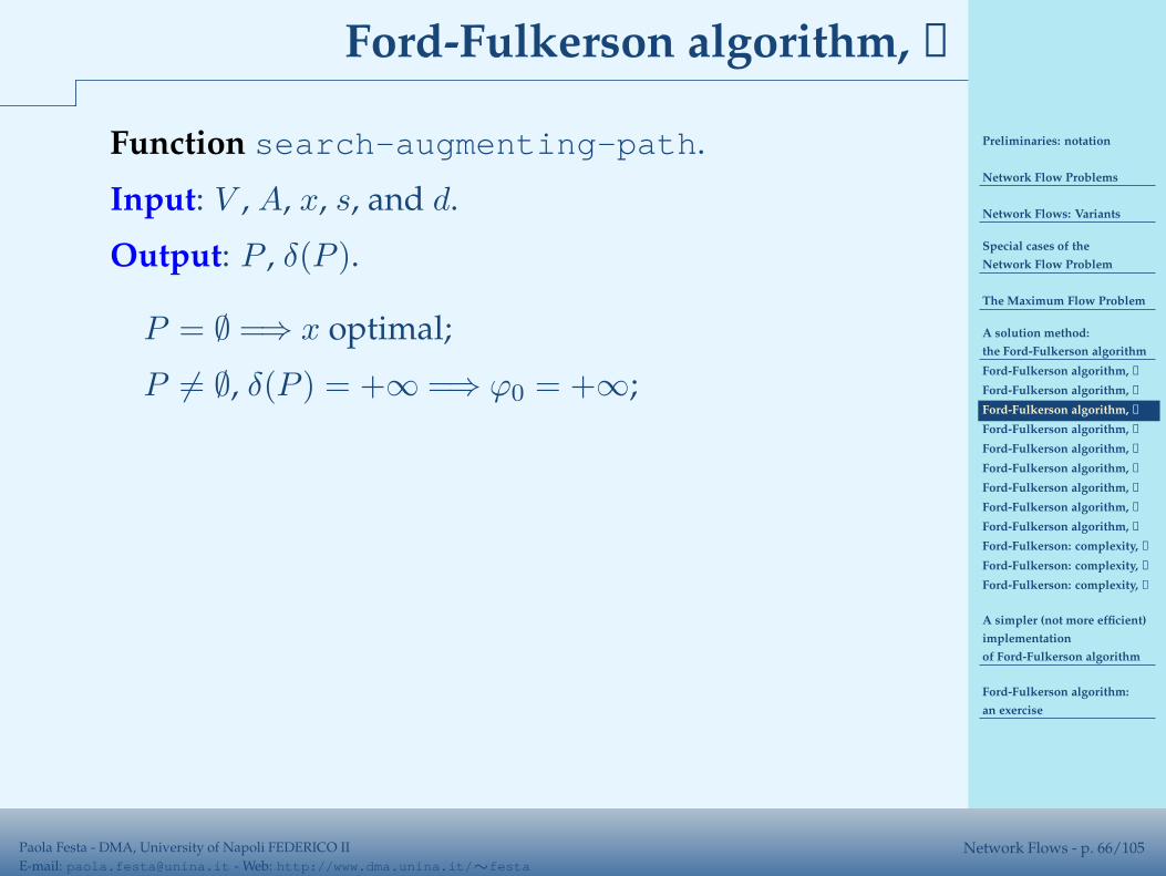
P 6= ∅, δ(P ) = +∞ =⇒ ϕ0 = +∞;
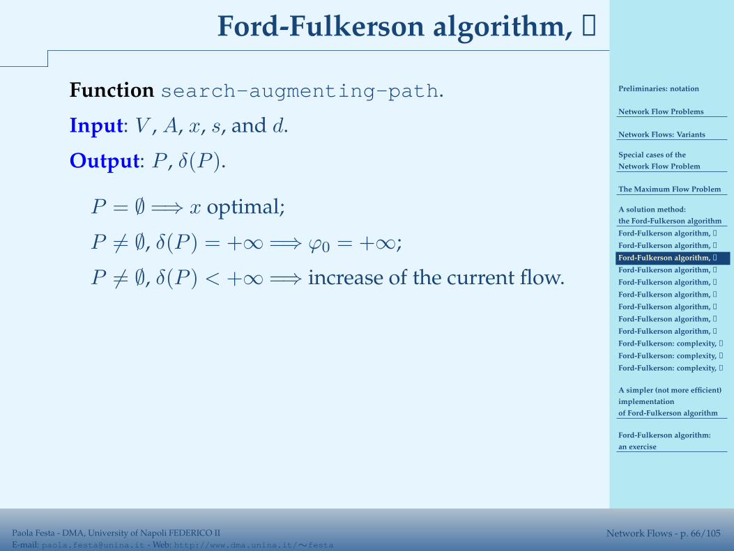
P 6= ∅, δ(P ) < +∞ =⇒ increase of the current flow.
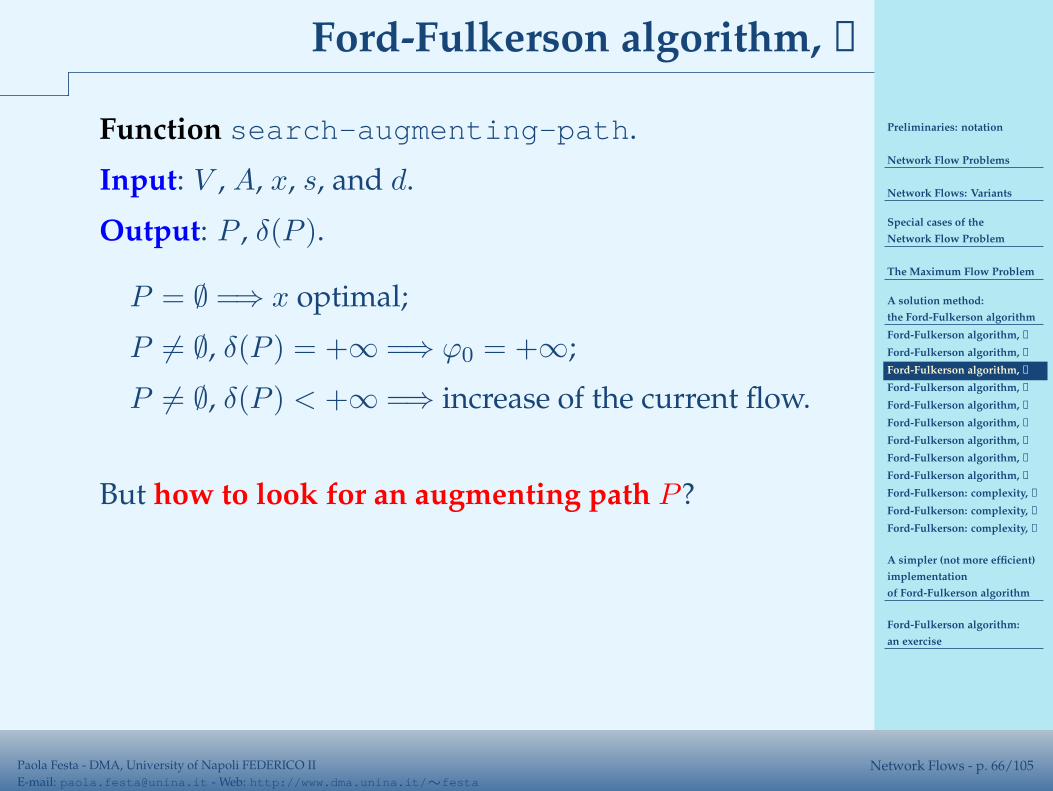
But how to look for an augmenting path P ?
It is used a labeling algorithm, that is a variant of a visitof the flow network N starting from the source s.
Preliminaries: notation
Network Flow Problems
Network Flows: Variants
Special cases of the
Network Flow Problem
The Maximum Flow Problem
A solution method:
the Ford-Fulkerson algorithm
Ford-Fulkerson algorithm, ➀
Ford-Fulkerson algorithm, ➁
Ford-Fulkerson algorithm, ➂
Ford-Fulkerson algorithm, ➂
Ford-Fulkerson algorithm, ➂
Ford-Fulkerson algorithm, ➂
Ford-Fulkerson algorithm, ➃
Ford-Fulkerson algorithm, ➃
Ford-Fulkerson algorithm, ➃
Ford-Fulkerson: complexity, ➀
Ford-Fulkerson: complexity, ➁
Ford-Fulkerson: complexity, ➂
A simpler (not more efficient)
implementation
of Ford-Fulkerson algorithm
Ford-Fulkerson algorithm:
an exercise
Paola Festa - DMA, University of Napoli FEDERICO II
E-mail: [email protected] - Web: http://www.dma.unina.it/∼festaNetwork Flows - p. 67/105
Ford-Fulkerson algorithm, ➂
Let x be a feasible flow and let P be a partial path P
from s to a node l ∈ V such that
✔ p(·) predecessor array in P (p(s) = s);
✔ ∀ (i, j) ∈ F (forward arc in P ), xij < kij andp(j) = i;
✔ ∀ (i, j) ∈ B (backward arc in B), xij > 0 andp(i) = j.
In this case, P is said partial augmenting path from s
to l and visiting labeled nodes.
Starting from the labeled node l, 2 cases can occur:
① ∃ an arc (l, j) ∈ A s.t. xlj < klj :it is possible to extend path P to include theforward arc (l, j), so obtaining a partialaugmenting path from s to node j, that becomeslabeled and p(j) := l;
Preliminaries: notation
Network Flow Problems
Network Flows: Variants
Special cases of the
Network Flow Problem
The Maximum Flow Problem
A solution method:
the Ford-Fulkerson algorithm
Ford-Fulkerson algorithm, ➀
Ford-Fulkerson algorithm, ➁
Ford-Fulkerson algorithm, ➂
Ford-Fulkerson algorithm, ➂
Ford-Fulkerson algorithm, ➂
Ford-Fulkerson algorithm, ➂
Ford-Fulkerson algorithm, ➃
Ford-Fulkerson algorithm, ➃
Ford-Fulkerson algorithm, ➃
Ford-Fulkerson: complexity, ➀
Ford-Fulkerson: complexity, ➁
Ford-Fulkerson: complexity, ➂
A simpler (not more efficient)
implementation
of Ford-Fulkerson algorithm
Ford-Fulkerson algorithm:
an exercise
Paola Festa - DMA, University of Napoli FEDERICO II
E-mail: [email protected] - Web: http://www.dma.unina.it/∼festaNetwork Flows - p. 68/105
Ford-Fulkerson algorithm, ➂
Let x be a feasible flow and let P be a partial path P
from s to a node l ∈ V such that
✔ p(·) predecessor array in P (p(s) = s);
✔ ∀ (i, j) ∈ F (forward arc in P ), xij < kij andp(j) = i;
✔ ∀ (i, j) ∈ B (backward arc in B), xij > 0 andp(i) = j.
In this case, P is said partial augmenting path from s
to l and visiting labeled nodes.
Starting from the labeled node l, 2 cases can occur:
② ∃ an arc (i, l) ∈ A s.t. xil > 0:it is possible to extend path P to include thebackward arc (i, l), so obtaining a partialaugmenting path from s to node i, that becomeslabeled and p(i) := l.
Preliminaries: notation
Network Flow Problems
Network Flows: Variants
Special cases of the
Network Flow Problem
The Maximum Flow Problem
A solution method:
the Ford-Fulkerson algorithm
Ford-Fulkerson algorithm, ➀
Ford-Fulkerson algorithm, ➁
Ford-Fulkerson algorithm, ➂
Ford-Fulkerson algorithm, ➂
Ford-Fulkerson algorithm, ➂
Ford-Fulkerson algorithm, ➂
Ford-Fulkerson algorithm, ➃
Ford-Fulkerson algorithm, ➃
Ford-Fulkerson algorithm, ➃
Ford-Fulkerson: complexity, ➀
Ford-Fulkerson: complexity, ➁
Ford-Fulkerson: complexity, ➂
A simpler (not more efficient)
implementation
of Ford-Fulkerson algorithm
Ford-Fulkerson algorithm:
an exercise
Paola Festa - DMA, University of Napoli FEDERICO II
E-mail: [email protected] - Web: http://www.dma.unina.it/∼festaNetwork Flows - p. 69/105
Ford-Fulkerson algorithm, ➂
search-augmenting-path stops when
✗ node d is labeled:
in this case, an augmenting path P from the sources to the sink d has been found and it can be builtby means of the predecessor array p;
or
✗ all labeled nodes are processed and the sink node d
results not labeled:
in this case, ∄ an augmenting path P from thesource s to the sink d.
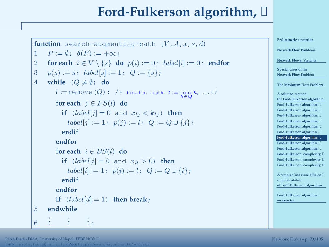
Preliminaries: notation
Network Flow Problems
Network Flows: Variants
Special cases of the
Network Flow Problem
The Maximum Flow Problem
A solution method:
the Ford-Fulkerson algorithm
Ford-Fulkerson algorithm, ➀
Ford-Fulkerson algorithm, ➁
Ford-Fulkerson algorithm, ➂
Ford-Fulkerson algorithm, ➂
Ford-Fulkerson algorithm, ➂
Ford-Fulkerson algorithm, ➂
Ford-Fulkerson algorithm, ➃
Ford-Fulkerson algorithm, ➃
Ford-Fulkerson algorithm, ➃
Ford-Fulkerson: complexity, ➀
Ford-Fulkerson: complexity, ➁
Ford-Fulkerson: complexity, ➂
A simpler (not more efficient)
implementation
of Ford-Fulkerson algorithm
Ford-Fulkerson algorithm:
an exercise
Paola Festa - DMA, University of Napoli FEDERICO II
E-mail: [email protected] - Web: http://www.dma.unina.it/∼festaNetwork Flows - p. 70/105
Ford-Fulkerson algorithm, ➃
function search-augmenting-path (V ,A,x,s,d)
1 P := ∅; δ(P ) := +∞;
2 for each i ∈ V \ {s} do p(i) := 0; label[i] := 0; endfor
3 p(s) := s; label[s] := 1; Q := {s};
4 while (Q 6= ∅) do
l :=remove(Q); /* breadth, depth, l := minh∈Q
h, ...*/
for each j ∈ FS(l) do
if (label[j] = 0 and xlj < klj) then
label[j] := 1; p(j) := l; Q := Q ∪ {j};
endif
endfor
for each i ∈ BS(l) do
if (label[i] = 0 and xil > 0) then
label[i] := 1; p(i) := l; Q := Q ∪ {i};
endif
endfor
if (label[d] = 1) then break;
5 endwhile
6...
......;
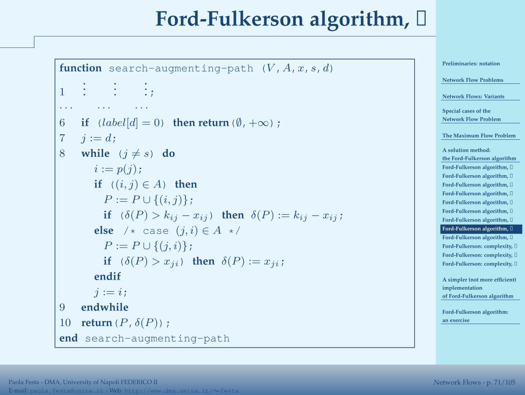
Preliminaries: notation
Network Flow Problems
Network Flows: Variants
Special cases of the
Network Flow Problem
The Maximum Flow Problem
A solution method:
the Ford-Fulkerson algorithm
Ford-Fulkerson algorithm, ➀
Ford-Fulkerson algorithm, ➁
Ford-Fulkerson algorithm, ➂
Ford-Fulkerson algorithm, ➂
Ford-Fulkerson algorithm, ➂
Ford-Fulkerson algorithm, ➂
Ford-Fulkerson algorithm, ➃
Ford-Fulkerson algorithm, ➃
Ford-Fulkerson algorithm, ➃
Ford-Fulkerson: complexity, ➀
Ford-Fulkerson: complexity, ➁
Ford-Fulkerson: complexity, ➂
A simpler (not more efficient)
implementation
of Ford-Fulkerson algorithm
Ford-Fulkerson algorithm:
an exercise
Paola Festa - DMA, University of Napoli FEDERICO II
E-mail: [email protected] - Web: http://www.dma.unina.it/∼festaNetwork Flows - p. 71/105
Ford-Fulkerson algorithm, ➃
function search-augmenting-path (V ,A,x,s,d)
1...
......;
· · · · · · · · ·
6 if (label[d] = 0) then return(∅,+∞);
7 j := d;
8 while (j 6= s) do
i := p(j);
if ((i, j) ∈ A) then
P := P ∪ {(i, j)};
if (δ(P ) > kij − xij) then δ(P ) := kij − xij;
else /* case (j, i) ∈ A */
P := P ∪ {(j, i)};
if (δ(P ) > xji) then δ(P ) := xji;
endif
j := i;
9 endwhile
10 return(P,δ(P ));
end search-augmenting-path
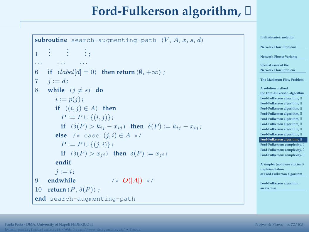
Preliminaries: notation
Network Flow Problems
Network Flows: Variants
Special cases of the
Network Flow Problem
The Maximum Flow Problem
A solution method:
the Ford-Fulkerson algorithm
Ford-Fulkerson algorithm, ➀
Ford-Fulkerson algorithm, ➁
Ford-Fulkerson algorithm, ➂
Ford-Fulkerson algorithm, ➂
Ford-Fulkerson algorithm, ➂
Ford-Fulkerson algorithm, ➂
Ford-Fulkerson algorithm, ➃
Ford-Fulkerson algorithm, ➃
Ford-Fulkerson algorithm, ➃
Ford-Fulkerson: complexity, ➀
Ford-Fulkerson: complexity, ➁
Ford-Fulkerson: complexity, ➂
A simpler (not more efficient)
implementation
of Ford-Fulkerson algorithm
Ford-Fulkerson algorithm:
an exercise
Paola Festa - DMA, University of Napoli FEDERICO II
E-mail: [email protected] - Web: http://www.dma.unina.it/∼festaNetwork Flows - p. 72/105
Ford-Fulkerson algorithm, ➃
subroutine search-augmenting-path (V ,A,x,s,d)
1...
......;
· · · · · · · · ·
6 if (label[d] = 0) then return(∅,+∞);
7 j := d;
8 while (j 6= s) do
i := p(j);
if ((i, j) ∈ A) then
P := P ∪ {(i, j)};
if (δ(P ) > kij − xij) then δ(P ) := kij − xij;
else /* case (j, i) ∈ A */
P := P ∪ {(j, i)};
if (δ(P ) > xji) then δ(P ) := xji;
endif
j := i;
9 endwhile /* O(|A|) */
10 return(P,δ(P ));
end search-augmenting-path
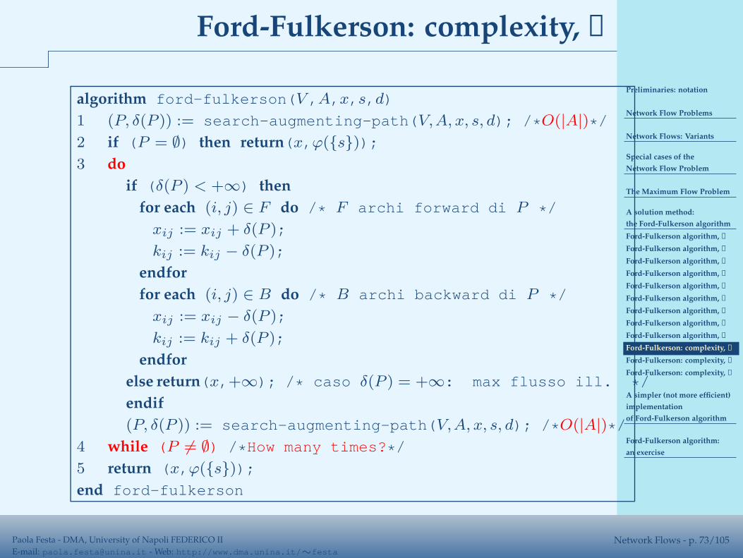
Preliminaries: notation
Network Flow Problems
Network Flows: Variants
Special cases of the
Network Flow Problem
The Maximum Flow Problem
A solution method:
the Ford-Fulkerson algorithm
Ford-Fulkerson algorithm, ➀
Ford-Fulkerson algorithm, ➁
Ford-Fulkerson algorithm, ➂
Ford-Fulkerson algorithm, ➂
Ford-Fulkerson algorithm, ➂
Ford-Fulkerson algorithm, ➂
Ford-Fulkerson algorithm, ➃
Ford-Fulkerson algorithm, ➃
Ford-Fulkerson algorithm, ➃
Ford-Fulkerson: complexity, ➀
Ford-Fulkerson: complexity, ➁
Ford-Fulkerson: complexity, ➂
A simpler (not more efficient)
implementation
of Ford-Fulkerson algorithm
Ford-Fulkerson algorithm:
an exercise
Paola Festa - DMA, University of Napoli FEDERICO II
E-mail: [email protected] - Web: http://www.dma.unina.it/∼festaNetwork Flows - p. 73/105
Ford-Fulkerson: complexity, ➀
algorithm ford-fulkerson(V ,A,x,s,d)
1 (P, δ(P )) := search-augmenting-path(V,A, x, s, d); /*O(|A|)*/
2 if (P = ∅) then return(x,ϕ({s}));
3 do
if (δ(P ) < +∞) then
for each (i, j) ∈ F do /* F archi forward di P */
xij := xij + δ(P );
kij := kij − δ(P );
endfor
for each (i, j) ∈ B do /* B archi backward di P */
xij := xij − δ(P );
kij := kij + δ(P );
endfor
else return(x,+∞); /* caso δ(P ) = +∞: max flusso ill. */
endif
(P, δ(P )) := search-augmenting-path(V,A, x, s, d); /*O(|A|)*/
4 while (P 6= ∅) /*How many times?*/
5 return (x,ϕ({s}));
end ford-fulkerson

Preliminaries: notation
Network Flow Problems
Network Flows: Variants
Special cases of the
Network Flow Problem
The Maximum Flow Problem
A solution method:
the Ford-Fulkerson algorithm
Ford-Fulkerson algorithm, ➀
Ford-Fulkerson algorithm, ➁
Ford-Fulkerson algorithm, ➂
Ford-Fulkerson algorithm, ➂
Ford-Fulkerson algorithm, ➂
Ford-Fulkerson algorithm, ➂
Ford-Fulkerson algorithm, ➃
Ford-Fulkerson algorithm, ➃
Ford-Fulkerson algorithm, ➃
Ford-Fulkerson: complexity, ➀
Ford-Fulkerson: complexity, ➁
Ford-Fulkerson: complexity, ➂
A simpler (not more efficient)
implementation
of Ford-Fulkerson algorithm
Ford-Fulkerson algorithm:
an exercise
Paola Festa - DMA, University of Napoli FEDERICO II
E-mail: [email protected] - Web: http://www.dma.unina.it/∼festaNetwork Flows - p. 74/105
Ford-Fulkerson: complexity, ➁
ford-fulkerson: nr of iterations in the worst case.
At each iteration, ϕ0 = ϕ({s}) is augmented in a strictlymonotone manner and the increment is δ(P ) > 0.
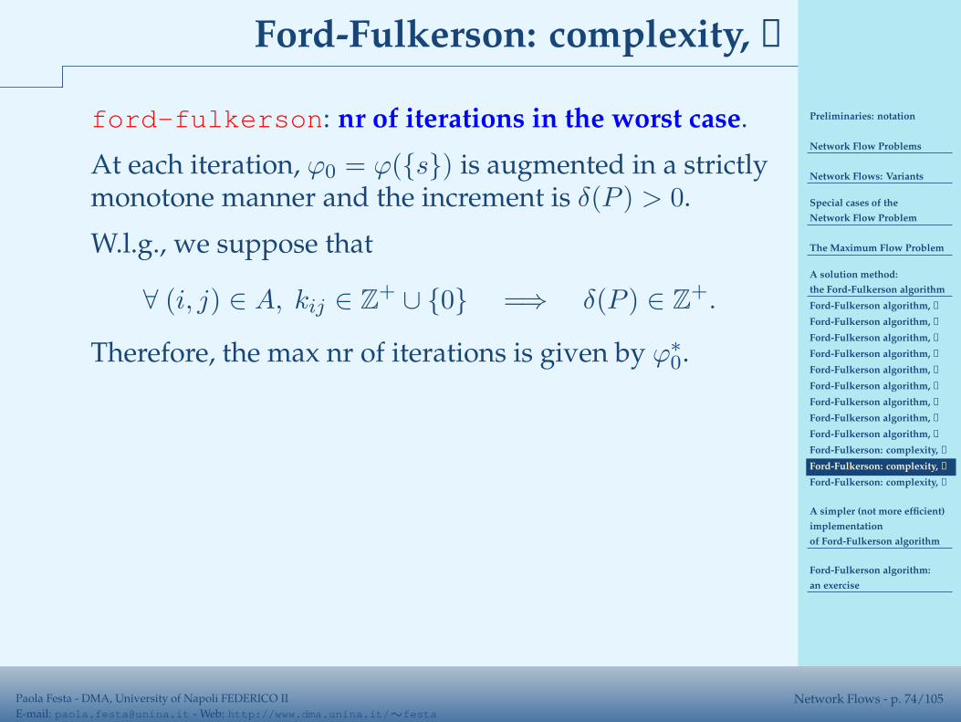
W.l.g., we suppose that
∀ (i, j) ∈ A, kij ∈ Z+ ∪ {0} =⇒ δ(P ) ∈ Z+.
Therefore, the max nr of iterations is given by ϕ∗0.
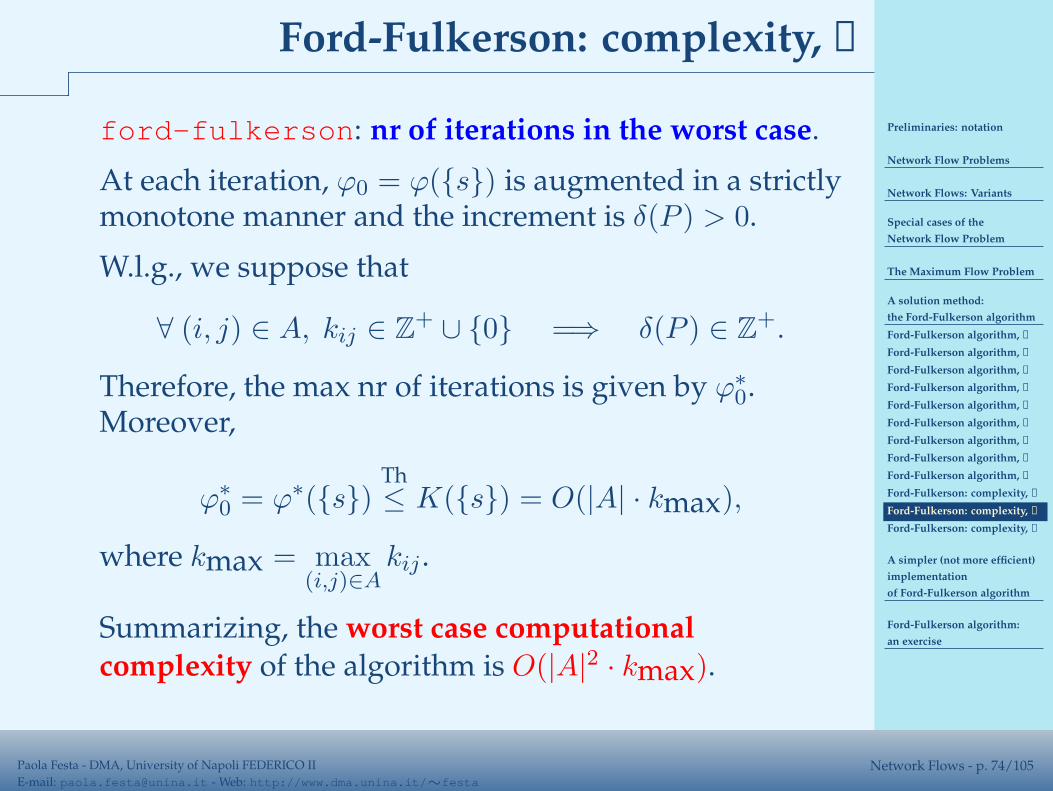
Moreover,
ϕ∗0 = ϕ∗({s})
Th≤ K({s}) = O(|A| · kmax),
where kmax = max(i,j)∈A
kij .
Summarizing, the worst case computational
complexity of the algorithm is O(|A|2 · kmax).
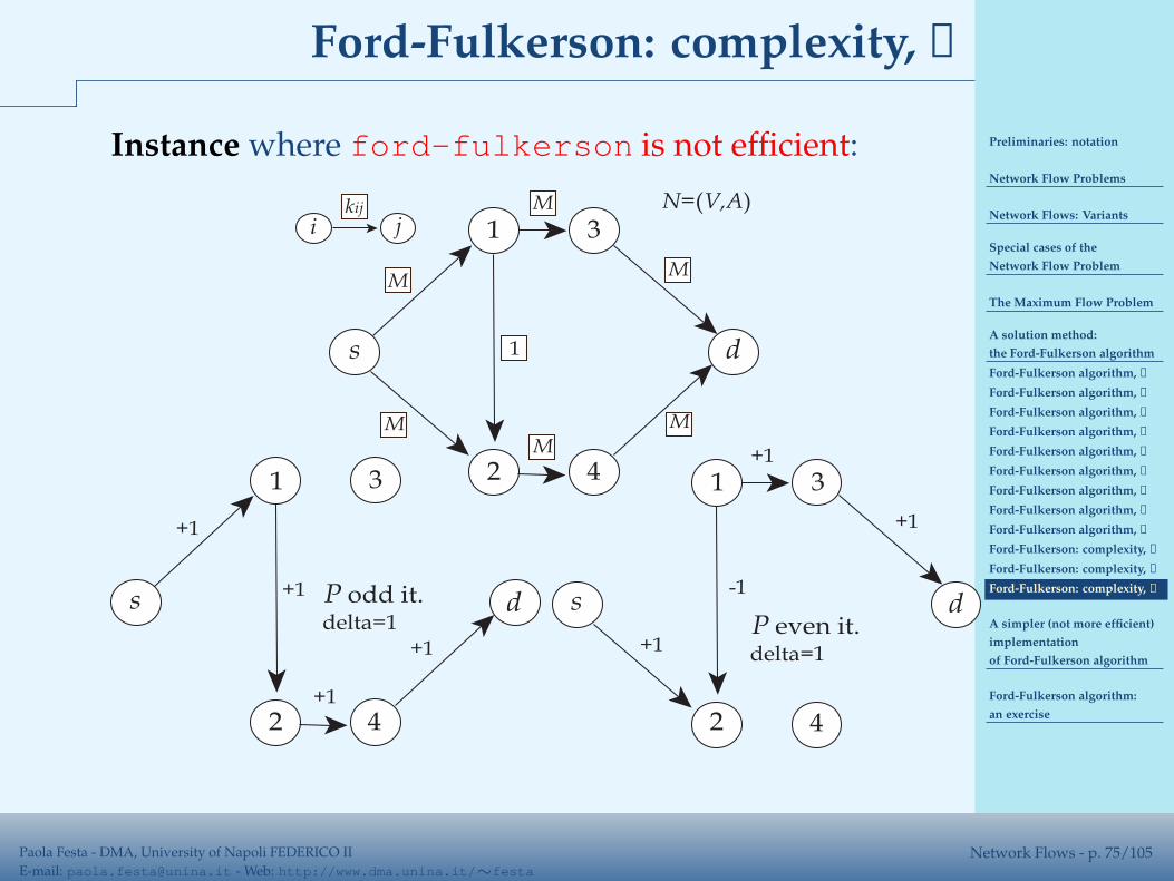
Preliminaries: notation
Network Flow Problems
Network Flows: Variants
Special cases of the
Network Flow Problem
The Maximum Flow Problem
A solution method:
the Ford-Fulkerson algorithm
Ford-Fulkerson algorithm, ➀
Ford-Fulkerson algorithm, ➁
Ford-Fulkerson algorithm, ➂
Ford-Fulkerson algorithm, ➂
Ford-Fulkerson algorithm, ➂
Ford-Fulkerson algorithm, ➂
Ford-Fulkerson algorithm, ➃
Ford-Fulkerson algorithm, ➃
Ford-Fulkerson algorithm, ➃
Ford-Fulkerson: complexity, ➀
Ford-Fulkerson: complexity, ➁
Ford-Fulkerson: complexity, ➂
A simpler (not more efficient)
implementation
of Ford-Fulkerson algorithm
Ford-Fulkerson algorithm:
an exercise
Paola Festa - DMA, University of Napoli FEDERICO II
E-mail: [email protected] - Web: http://www.dma.unina.it/∼festaNetwork Flows - p. 75/105
Ford-Fulkerson: complexity, ➂
Instance where ford-fulkerson is not efficient:
s
1
d
2
1
M
ikij
j 3
4
MM
M
M
M N=(V,A)
s
1
d
2
3
4
s
1
d
2
3
4
P odd it.delta=1
+1
+1
+1
+1 +1
+1
+1
-1
P even it.delta=1
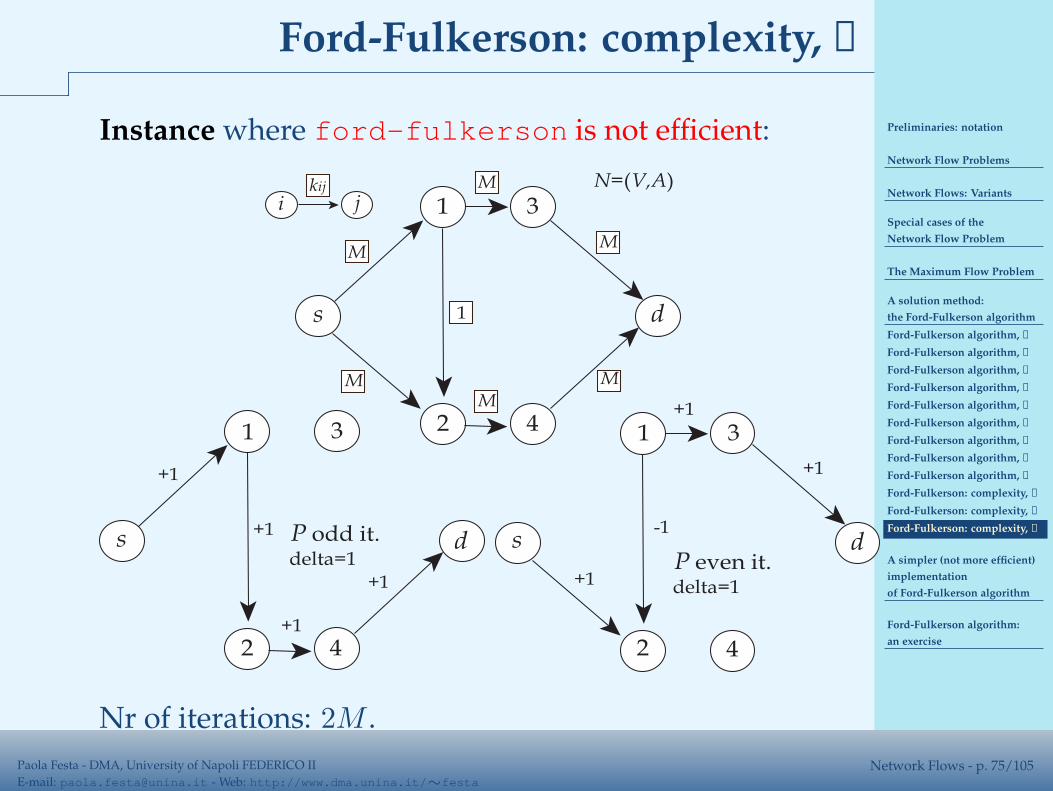
Nr of iterations: 2M .

Preliminaries: notation
Network Flow Problems
Network Flows: Variants
Special cases of the
Network Flow Problem
The Maximum Flow Problem
A solution method:
the Ford-Fulkerson algorithm
A simpler (not more efficient)
implementation
of Ford-Fulkerson algorithm
Ford-Fulkerson 2, ➀
Ford-Fulkerson 2, ➁
Ford-Fulkerson 2, ➁
Ford-Fulkerson algorithm:
an exercise
Paola Festa - DMA, University of Napoli FEDERICO II
E-mail: [email protected] - Web: http://www.dma.unina.it/∼festaNetwork Flows - p. 76/105
A simpler (not more efficient)implementation
of Ford-Fulkerson algorithm
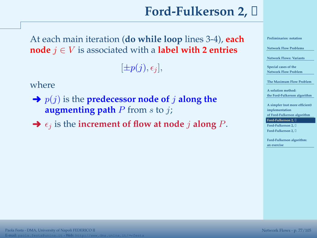
Preliminaries: notation
Network Flow Problems
Network Flows: Variants
Special cases of the
Network Flow Problem
The Maximum Flow Problem
A solution method:
the Ford-Fulkerson algorithm
A simpler (not more efficient)
implementation
of Ford-Fulkerson algorithm
Ford-Fulkerson 2, ➀
Ford-Fulkerson 2, ➁
Ford-Fulkerson 2, ➁
Ford-Fulkerson algorithm:
an exercise
Paola Festa - DMA, University of Napoli FEDERICO II
E-mail: [email protected] - Web: http://www.dma.unina.it/∼festaNetwork Flows - p. 77/105
Ford-Fulkerson 2, ➀
At each main iteration (do while loop lines 3-4), eachnode j ∈ V is associated with a label with 2 entries
[±p(j), ǫj ],
where
➜ p(j) is the predecessor node of j along theaugmenting path P from s to j;
➜ ǫj is the increment of flow at node j along P .
✍ “+”=⇒ j is reached traversing the forward arc(p(j), j) ∈ A;
✍ “−”=⇒ j is reached traversing the backward arc(j, p(j)) ∈ A.
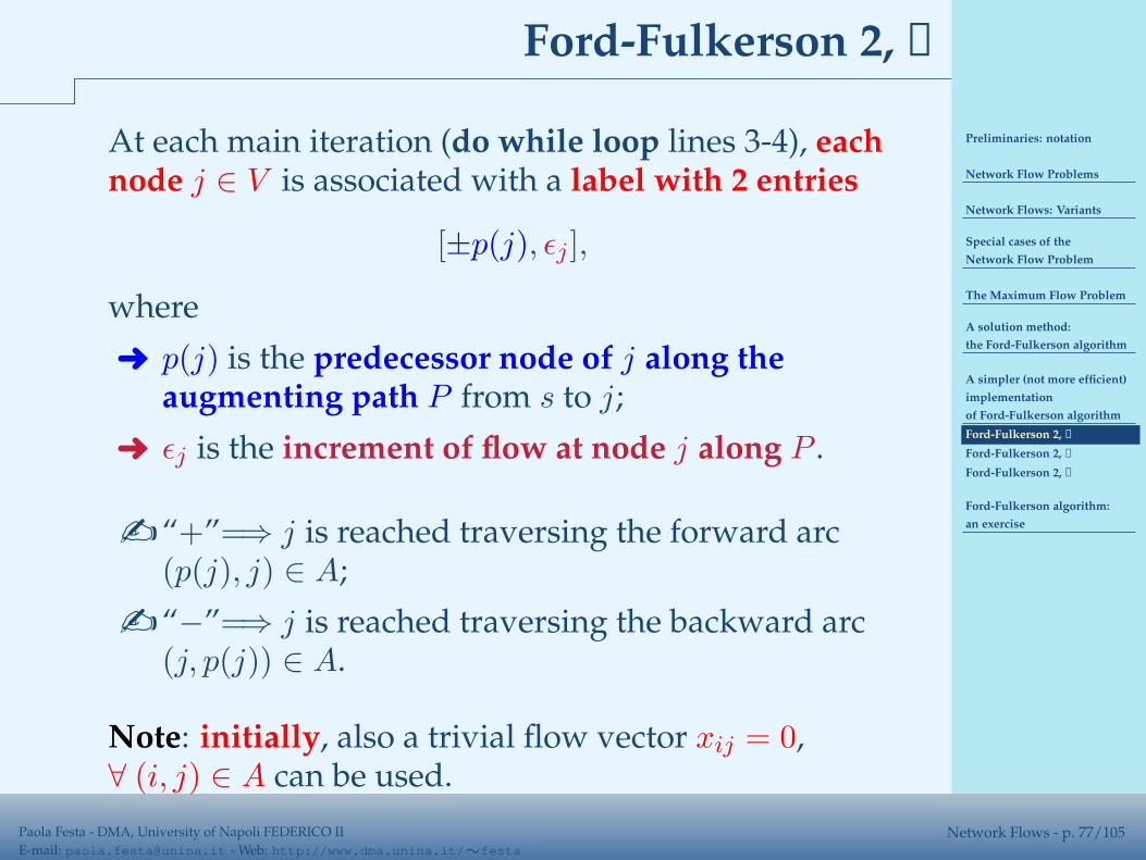
Note: initially, also a trivial flow vector xij = 0,∀ (i, j) ∈ A can be used.
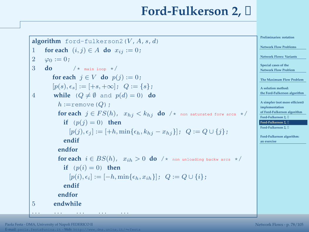
Preliminaries: notation
Network Flow Problems
Network Flows: Variants
Special cases of the
Network Flow Problem
The Maximum Flow Problem
A solution method:
the Ford-Fulkerson algorithm
A simpler (not more efficient)
implementation
of Ford-Fulkerson algorithm
Ford-Fulkerson 2, ➀
Ford-Fulkerson 2, ➁
Ford-Fulkerson 2, ➁
Ford-Fulkerson algorithm:
an exercise
Paola Festa - DMA, University of Napoli FEDERICO II
E-mail: [email protected] - Web: http://www.dma.unina.it/∼festaNetwork Flows - p. 78/105
Ford-Fulkerson 2, ➁
algorithm ford-fulkerson2(V ,A,s,d)
1 for each (i, j) ∈ A do xij := 0;
2 ϕ0 := 0;
3 do /* main loop */
for each j ∈ V do p(j) := 0;
[p(s), ǫs] := [+s,+∞]; Q := {s};
4 while (Q 6= ∅ and p(d) = 0) do
h :=remove(Q);
for each j ∈ FS(h), xhj < khj do /* non saturated forw arcs */
if (p(j) = 0) then
[p(j), ǫj ] := [+h, min{ǫh, khj − xhj}]; Q := Q ∪ {j};
endif
endfor
for each i ∈ BS(h), xih > 0 do /* non unloading backw arcs */
if (p(i) = 0) then
[p(i), ǫi] := [−h, min{ǫh, xih}]; Q := Q ∪ {i};
endif
endfor
5 endwhile
· · · · · · · · · · · · · · ·
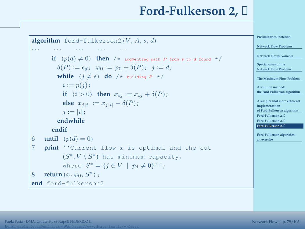
Preliminaries: notation
Network Flow Problems
Network Flows: Variants
Special cases of the
Network Flow Problem
The Maximum Flow Problem
A solution method:
the Ford-Fulkerson algorithm
A simpler (not more efficient)
implementation
of Ford-Fulkerson algorithm
Ford-Fulkerson 2, ➀
Ford-Fulkerson 2, ➁
Ford-Fulkerson 2, ➁
Ford-Fulkerson algorithm:
an exercise
Paola Festa - DMA, University of Napoli FEDERICO II
E-mail: [email protected] - Web: http://www.dma.unina.it/∼festaNetwork Flows - p. 79/105
Ford-Fulkerson 2, ➁
algorithm ford-fulkerson2(V ,A,s,d)
· · · · · · · · · · · · · · ·
if (p(d) 6= 0) then /* augmenting path P from s to d found */
δ(P ) := ǫd; ϕ0 := ϕ0 + δ(P ); j := d;
while (j 6= s) do /* building P */
i := p(j);
if (i > 0) then xij := xij + δ(P );
else xj|i| := xj|i| − δ(P );
j := |i|;
endwhile
endif
6 until (p(d) = 0)
7 print ‘‘Current flow x is optimal and the cut
(S∗, V \ S∗) has minimum capacity,
where S∗ = {j ∈ V | pj 6= 0}’’;
8 return(x,ϕ0,S∗);
end ford-fulkerson2

Preliminaries: notation
Network Flow Problems
Network Flows: Variants
Special cases of the
Network Flow Problem
The Maximum Flow Problem
A solution method:
the Ford-Fulkerson algorithm
A simpler (not more efficient)
implementation
of Ford-Fulkerson algorithm
Ford-Fulkerson algorithm:
an exercise
Exercise, ➀
Exercise, ➁
Exercise, ➂
Exercise, ➂
Exercise, ➂
Exercise, ➂
Exercise, ➂
Exercise, ➂
Exercise, ➂
Exercise, ➃
Exercise, ➃
Exercise, ➃
Exercise, ➃
Exercise, ➃
Exercise, ➃
Exercise, ➃
Exercise, ➃
Exercise, ➃
Exercise, ➃
Exercise, ➃
Exercise, ➄
Exercise, ➄
Paola Festa - DMA, University of Napoli FEDERICO II
E-mail: [email protected] - Web: http://www.dma.unina.it/∼festaNetwork Flows - p. 80/105
Ford-Fulkerson algorithm:an exercise
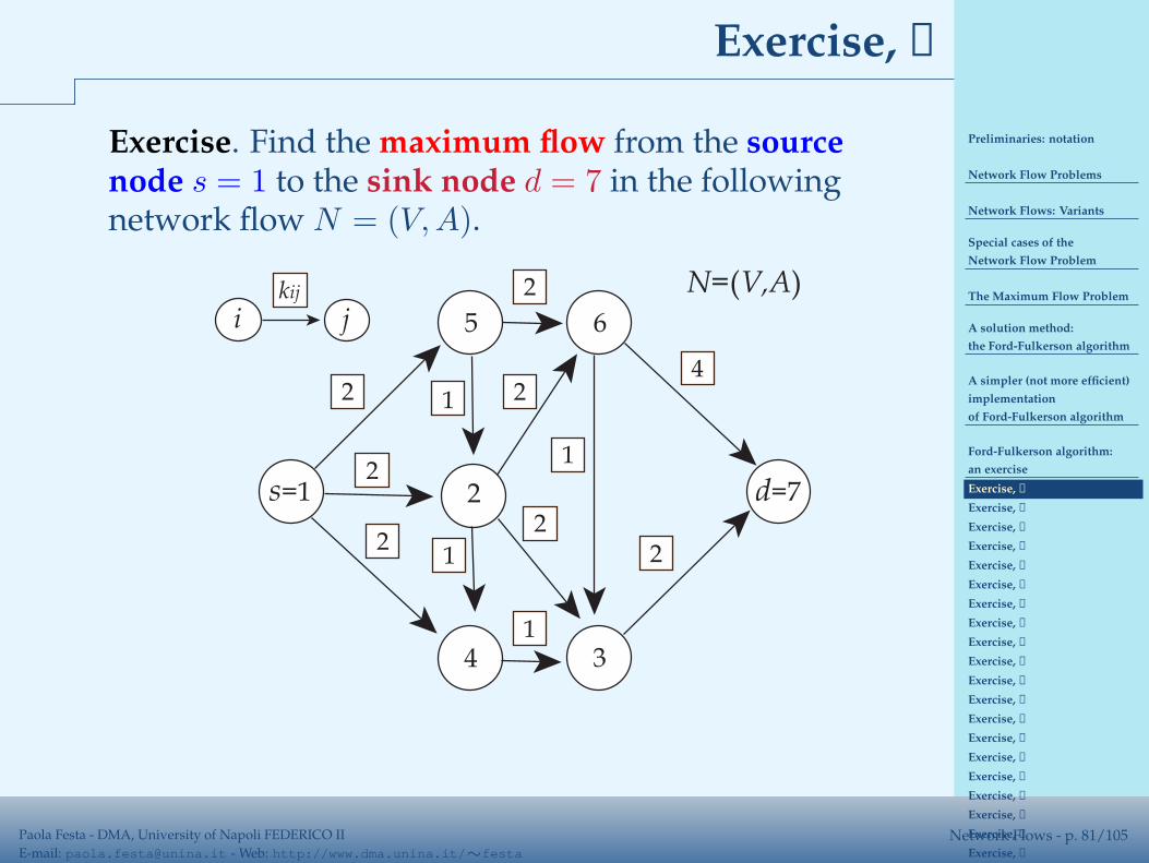
Preliminaries: notation
Network Flow Problems
Network Flows: Variants
Special cases of the
Network Flow Problem
The Maximum Flow Problem
A solution method:
the Ford-Fulkerson algorithm
A simpler (not more efficient)
implementation
of Ford-Fulkerson algorithm
Ford-Fulkerson algorithm:
an exercise
Exercise, ➀
Exercise, ➁
Exercise, ➂
Exercise, ➂
Exercise, ➂
Exercise, ➂
Exercise, ➂
Exercise, ➂
Exercise, ➂
Exercise, ➃
Exercise, ➃
Exercise, ➃
Exercise, ➃
Exercise, ➃
Exercise, ➃
Exercise, ➃
Exercise, ➃
Exercise, ➃
Exercise, ➃
Exercise, ➃
Exercise, ➄
Exercise, ➄
Paola Festa - DMA, University of Napoli FEDERICO II
E-mail: [email protected] - Web: http://www.dma.unina.it/∼festaNetwork Flows - p. 81/105
Exercise, ➀
Exercise. Find the maximum flow from the sourcenode s = 1 to the sink node d = 7 in the followingnetwork flow N = (V,A).
s=1
5
d=7
4
1
ikij
j 6
3
2
N=(V,A)
22
21
2
2
2
1
1
2
4
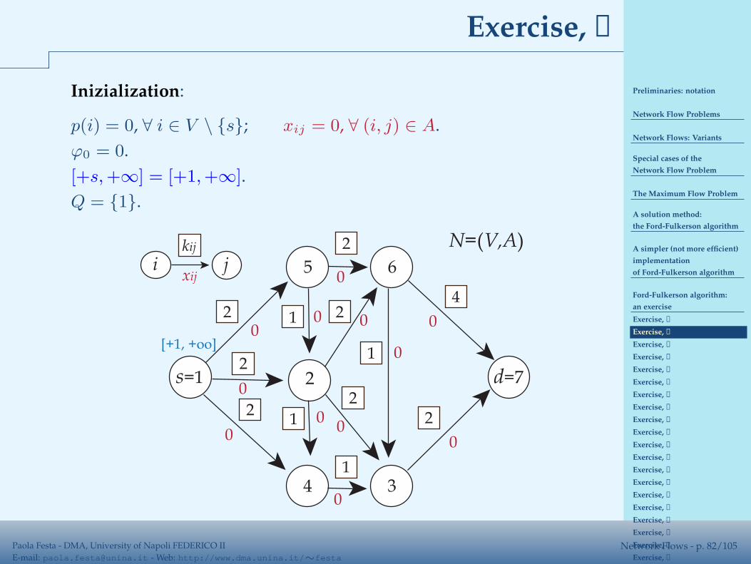
Preliminaries: notation
Network Flow Problems
Network Flows: Variants
Special cases of the
Network Flow Problem
The Maximum Flow Problem
A solution method:
the Ford-Fulkerson algorithm
A simpler (not more efficient)
implementation
of Ford-Fulkerson algorithm
Ford-Fulkerson algorithm:
an exercise
Exercise, ➀
Exercise, ➁
Exercise, ➂
Exercise, ➂
Exercise, ➂
Exercise, ➂
Exercise, ➂
Exercise, ➂
Exercise, ➂
Exercise, ➃
Exercise, ➃
Exercise, ➃
Exercise, ➃
Exercise, ➃
Exercise, ➃
Exercise, ➃
Exercise, ➃
Exercise, ➃
Exercise, ➃
Exercise, ➃
Exercise, ➄
Exercise, ➄
Paola Festa - DMA, University of Napoli FEDERICO II
E-mail: [email protected] - Web: http://www.dma.unina.it/∼festaNetwork Flows - p. 82/105
Exercise, ➁
Inizialization:
p(i) = 0, ∀ i ∈ V \ {s}; xij = 0, ∀ (i, j) ∈ A.
ϕ0 = 0.
[+s, +∞] = [+1,+∞].
Q = {1}.
s=1
5
d=7
4
1
ikij
j 6
3
2
N=(V,A)
22
21
2
2
2
1
1
2
4
0
0
0
0
0
0
0
0
00
0
0
xij
[+1, +oo]
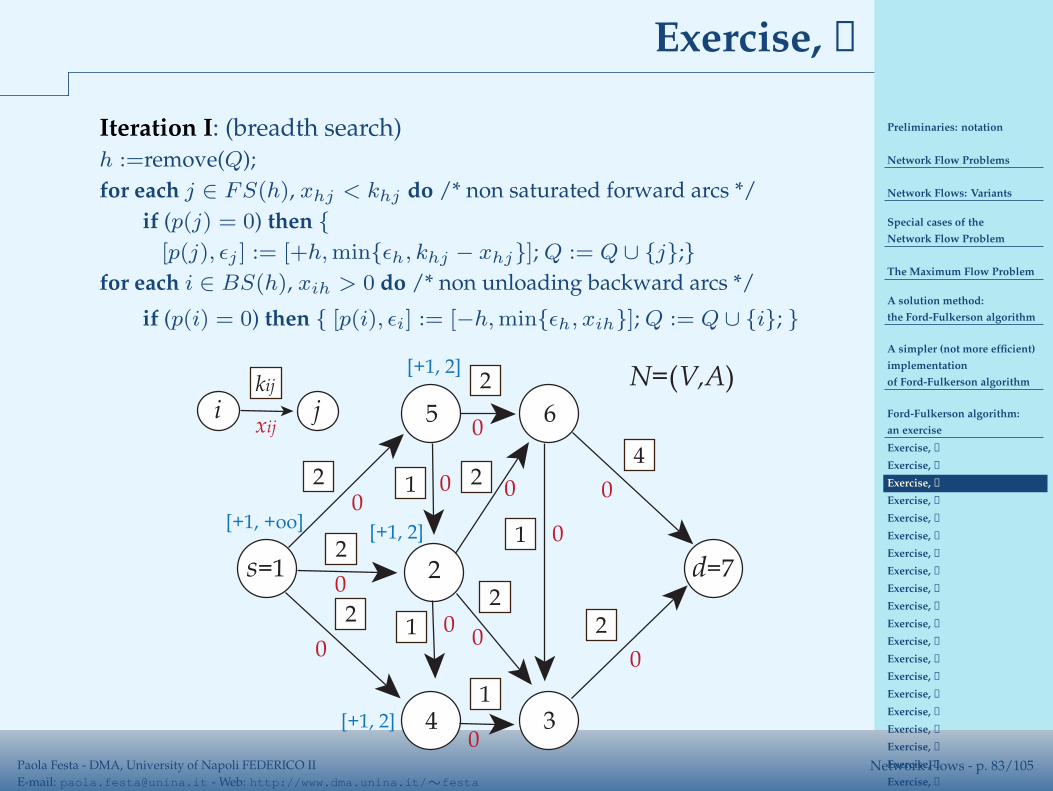
Preliminaries: notation
Network Flow Problems
Network Flows: Variants
Special cases of the
Network Flow Problem
The Maximum Flow Problem
A solution method:
the Ford-Fulkerson algorithm
A simpler (not more efficient)
implementation
of Ford-Fulkerson algorithm
Ford-Fulkerson algorithm:
an exercise
Exercise, ➀
Exercise, ➁
Exercise, ➂
Exercise, ➂
Exercise, ➂
Exercise, ➂
Exercise, ➂
Exercise, ➂
Exercise, ➂
Exercise, ➃
Exercise, ➃
Exercise, ➃
Exercise, ➃
Exercise, ➃
Exercise, ➃
Exercise, ➃
Exercise, ➃
Exercise, ➃
Exercise, ➃
Exercise, ➃
Exercise, ➄
Exercise, ➄
Paola Festa - DMA, University of Napoli FEDERICO II
E-mail: [email protected] - Web: http://www.dma.unina.it/∼festaNetwork Flows - p. 83/105
Exercise, ➂
Iteration I: (breadth search)h :=remove(Q);
for each j ∈ FS(h), xhj < khj do /* non saturated forward arcs */
if (p(j) = 0) then {
[p(j), ǫj ] := [+h, min{ǫh, khj − xhj}]; Q := Q ∪ {j};}
for each i ∈ BS(h), xih > 0 do /* non unloading backward arcs */
if (p(i) = 0) then { [p(i), ǫi] := [−h, min{ǫh, xih}]; Q := Q ∪ {i}; }
s=1
5
d=7
4
1
ikij
j 6
3
2
N=(V,A)
22
21
2
2
2
1
1
2
4
0
0
0
0
0
0
0
0
00
0
0
xij
[+1, +oo]
[+1, 2]
[+1, 2]
[+1, 2]

Preliminaries: notation
Network Flow Problems
Network Flows: Variants
Special cases of the
Network Flow Problem
The Maximum Flow Problem
A solution method:
the Ford-Fulkerson algorithm
A simpler (not more efficient)
implementation
of Ford-Fulkerson algorithm
Ford-Fulkerson algorithm:
an exercise
Exercise, ➀
Exercise, ➁
Exercise, ➂
Exercise, ➂
Exercise, ➂
Exercise, ➂
Exercise, ➂
Exercise, ➂
Exercise, ➂
Exercise, ➃
Exercise, ➃
Exercise, ➃
Exercise, ➃
Exercise, ➃
Exercise, ➃
Exercise, ➃
Exercise, ➃
Exercise, ➃
Exercise, ➃
Exercise, ➃
Exercise, ➄
Exercise, ➄
Paola Festa - DMA, University of Napoli FEDERICO II
E-mail: [email protected] - Web: http://www.dma.unina.it/∼festaNetwork Flows - p. 84/105
Exercise, ➂
Iteration I: (breadth search)h :=remove(Q);
for each j ∈ FS(h), xhj < khj do /* non saturated forward arcs */
if (p(j) = 0) then {
[p(j), ǫj ] := [+h, min{ǫh, khj − xhj}]; Q := Q ∪ {j};}
for each i ∈ BS(h), xih > 0 do /* non unloading backward arcs */
if (p(i) = 0) then { [p(i), ǫi] := [−h, min{ǫh, xih}]; Q := Q ∪ {i}; }
s=1
5
d=7
4
1
ikij
j 6
3
2
N=(V,A)
22
21
2
2
2
1
1
2
4
0
0
0
0
0
0
0
0
00
0
0
xij
[+1, +oo]
[+1, 2]
[+1, 2]
[+1, 2]
[+2, 2]
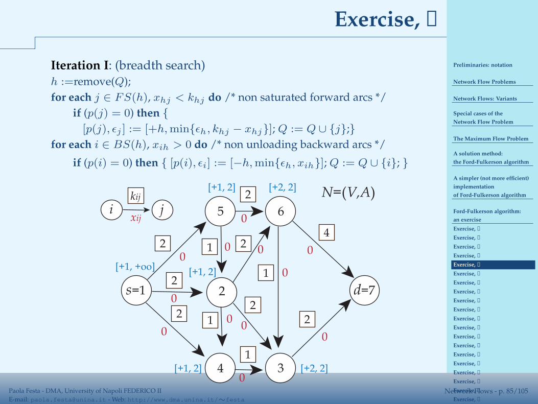
Preliminaries: notation
Network Flow Problems
Network Flows: Variants
Special cases of the
Network Flow Problem
The Maximum Flow Problem
A solution method:
the Ford-Fulkerson algorithm
A simpler (not more efficient)
implementation
of Ford-Fulkerson algorithm
Ford-Fulkerson algorithm:
an exercise
Exercise, ➀
Exercise, ➁
Exercise, ➂
Exercise, ➂
Exercise, ➂
Exercise, ➂
Exercise, ➂
Exercise, ➂
Exercise, ➂
Exercise, ➃
Exercise, ➃
Exercise, ➃
Exercise, ➃
Exercise, ➃
Exercise, ➃
Exercise, ➃
Exercise, ➃
Exercise, ➃
Exercise, ➃
Exercise, ➃
Exercise, ➄
Exercise, ➄
Paola Festa - DMA, University of Napoli FEDERICO II
E-mail: [email protected] - Web: http://www.dma.unina.it/∼festaNetwork Flows - p. 85/105
Exercise, ➂
Iteration I: (breadth search)h :=remove(Q);
for each j ∈ FS(h), xhj < khj do /* non saturated forward arcs */
if (p(j) = 0) then {
[p(j), ǫj ] := [+h, min{ǫh, khj − xhj}]; Q := Q ∪ {j};}
for each i ∈ BS(h), xih > 0 do /* non unloading backward arcs */
if (p(i) = 0) then { [p(i), ǫi] := [−h, min{ǫh, xih}]; Q := Q ∪ {i}; }
s=1
5
d=7
4
1
ikij
j 6
3
2
N=(V,A)
22
21
2
2
2
1
1
2
4
0
0
0
0
0
0
0
0
00
0
0
xij
[+1, +oo]
[+1, 2]
[+1, 2]
[+1, 2] [+2, 2]
[+2, 2]
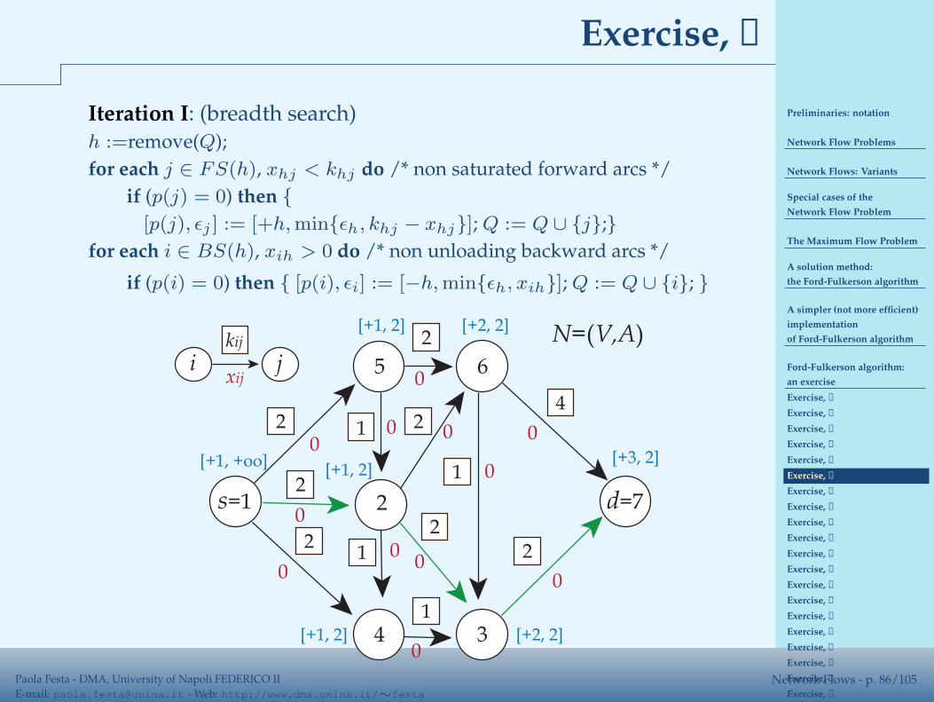
Preliminaries: notation
Network Flow Problems
Network Flows: Variants
Special cases of the
Network Flow Problem
The Maximum Flow Problem
A solution method:
the Ford-Fulkerson algorithm
A simpler (not more efficient)
implementation
of Ford-Fulkerson algorithm
Ford-Fulkerson algorithm:
an exercise
Exercise, ➀
Exercise, ➁
Exercise, ➂
Exercise, ➂
Exercise, ➂
Exercise, ➂
Exercise, ➂
Exercise, ➂
Exercise, ➂
Exercise, ➃
Exercise, ➃
Exercise, ➃
Exercise, ➃
Exercise, ➃
Exercise, ➃
Exercise, ➃
Exercise, ➃
Exercise, ➃
Exercise, ➃
Exercise, ➃
Exercise, ➄
Exercise, ➄
Paola Festa - DMA, University of Napoli FEDERICO II
E-mail: [email protected] - Web: http://www.dma.unina.it/∼festaNetwork Flows - p. 86/105
Exercise, ➂
Iteration I: (breadth search)h :=remove(Q);
for each j ∈ FS(h), xhj < khj do /* non saturated forward arcs */
if (p(j) = 0) then {
[p(j), ǫj ] := [+h, min{ǫh, khj − xhj}]; Q := Q ∪ {j};}
for each i ∈ BS(h), xih > 0 do /* non unloading backward arcs */
if (p(i) = 0) then { [p(i), ǫi] := [−h, min{ǫh, xih}]; Q := Q ∪ {i}; }
s=1
5
d=7
4
1
ikij
j 6
3
2
N=(V,A)
22
21
2
2
2
1
1
2
4
0
0
0
0
0
0
0
0
00
0
0
xij
[+1, +oo]
[+1, 2]
[+1, 2]
[+1, 2] [+2, 2]
[+2, 2]
[+3, 2]
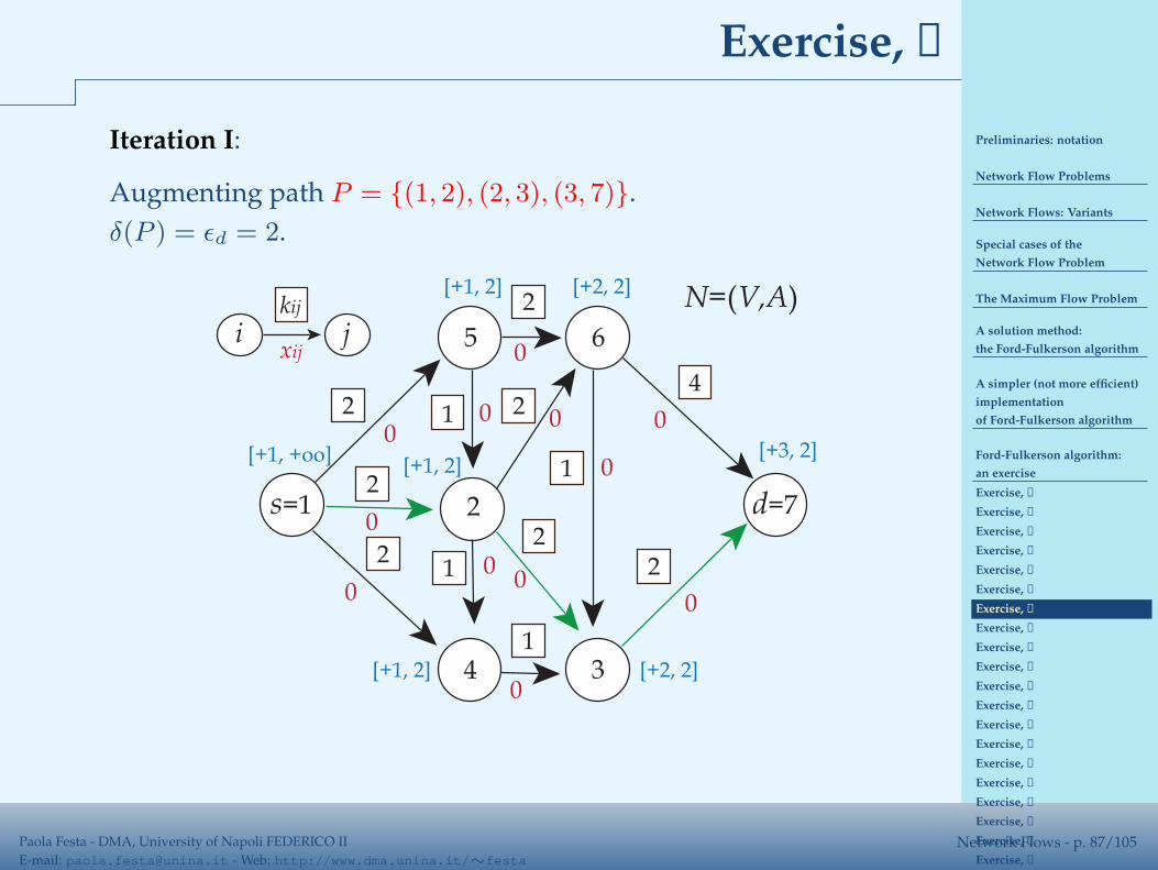
Preliminaries: notation
Network Flow Problems
Network Flows: Variants
Special cases of the
Network Flow Problem
The Maximum Flow Problem
A solution method:
the Ford-Fulkerson algorithm
A simpler (not more efficient)
implementation
of Ford-Fulkerson algorithm
Ford-Fulkerson algorithm:
an exercise
Exercise, ➀
Exercise, ➁
Exercise, ➂
Exercise, ➂
Exercise, ➂
Exercise, ➂
Exercise, ➂
Exercise, ➂
Exercise, ➂
Exercise, ➃
Exercise, ➃
Exercise, ➃
Exercise, ➃
Exercise, ➃
Exercise, ➃
Exercise, ➃
Exercise, ➃
Exercise, ➃
Exercise, ➃
Exercise, ➃
Exercise, ➄
Exercise, ➄
Paola Festa - DMA, University of Napoli FEDERICO II
E-mail: [email protected] - Web: http://www.dma.unina.it/∼festaNetwork Flows - p. 87/105
Exercise, ➂
Iteration I:
Augmenting path P = {(1, 2), (2, 3), (3, 7)}.
δ(P ) = ǫd = 2.
s=1
5
d=7
4
1
ikij
j 6
3
2
N=(V,A)
22
21
2
2
2
1
1
2
4
0
0
0
0
0
0
0
0
00
0
0
xij
[+1, +oo]
[+1, 2]
[+1, 2]
[+1, 2] [+2, 2]
[+2, 2]
[+3, 2]
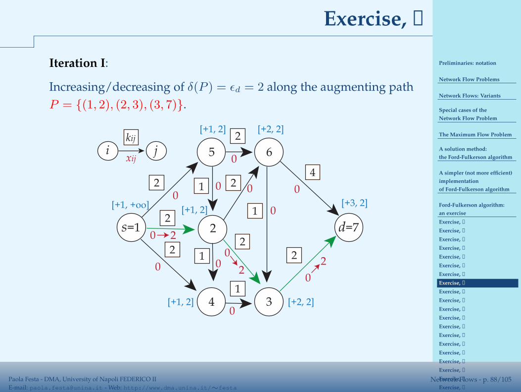
Preliminaries: notation
Network Flow Problems
Network Flows: Variants
Special cases of the
Network Flow Problem
The Maximum Flow Problem
A solution method:
the Ford-Fulkerson algorithm
A simpler (not more efficient)
implementation
of Ford-Fulkerson algorithm
Ford-Fulkerson algorithm:
an exercise
Exercise, ➀
Exercise, ➁
Exercise, ➂
Exercise, ➂
Exercise, ➂
Exercise, ➂
Exercise, ➂
Exercise, ➂
Exercise, ➂
Exercise, ➃
Exercise, ➃
Exercise, ➃
Exercise, ➃
Exercise, ➃
Exercise, ➃
Exercise, ➃
Exercise, ➃
Exercise, ➃
Exercise, ➃
Exercise, ➃
Exercise, ➄
Exercise, ➄
Paola Festa - DMA, University of Napoli FEDERICO II
E-mail: [email protected] - Web: http://www.dma.unina.it/∼festaNetwork Flows - p. 88/105
Exercise, ➂
Iteration I:
Increasing/decreasing of δ(P ) = ǫd = 2 along the augmenting path
P = {(1, 2), (2, 3), (3, 7)}.
s=1
5
d=7
4
1
ikij
j 6
3
2
22
21
2
2
2
1
1
2
4
0
0
0
0
0
0
0
0
00
0
0
xij
[+1, +oo]
[+1, 2]
[+1, 2]
[+1, 2] [+2, 2]
[+2, 2]
[+3, 2]
2
22
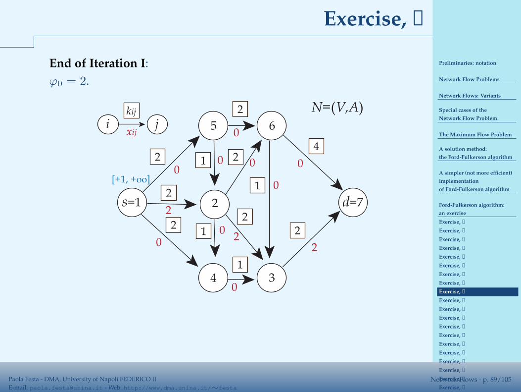
Preliminaries: notation
Network Flow Problems
Network Flows: Variants
Special cases of the
Network Flow Problem
The Maximum Flow Problem
A solution method:
the Ford-Fulkerson algorithm
A simpler (not more efficient)
implementation
of Ford-Fulkerson algorithm
Ford-Fulkerson algorithm:
an exercise
Exercise, ➀
Exercise, ➁
Exercise, ➂
Exercise, ➂
Exercise, ➂
Exercise, ➂
Exercise, ➂
Exercise, ➂
Exercise, ➂
Exercise, ➃
Exercise, ➃
Exercise, ➃
Exercise, ➃
Exercise, ➃
Exercise, ➃
Exercise, ➃
Exercise, ➃
Exercise, ➃
Exercise, ➃
Exercise, ➃
Exercise, ➄
Exercise, ➄
Paola Festa - DMA, University of Napoli FEDERICO II
E-mail: [email protected] - Web: http://www.dma.unina.it/∼festaNetwork Flows - p. 89/105
Exercise, ➂
End of Iteration I:
ϕ0 = 2.
s=1
5
d=7
4
1
ikij
j 6
3
2
N=(V,A)
22
21
2
2
2
1
1
2
4
0
2
0
0
0
0
0
0
02
0
2
xij
[+1, +oo]
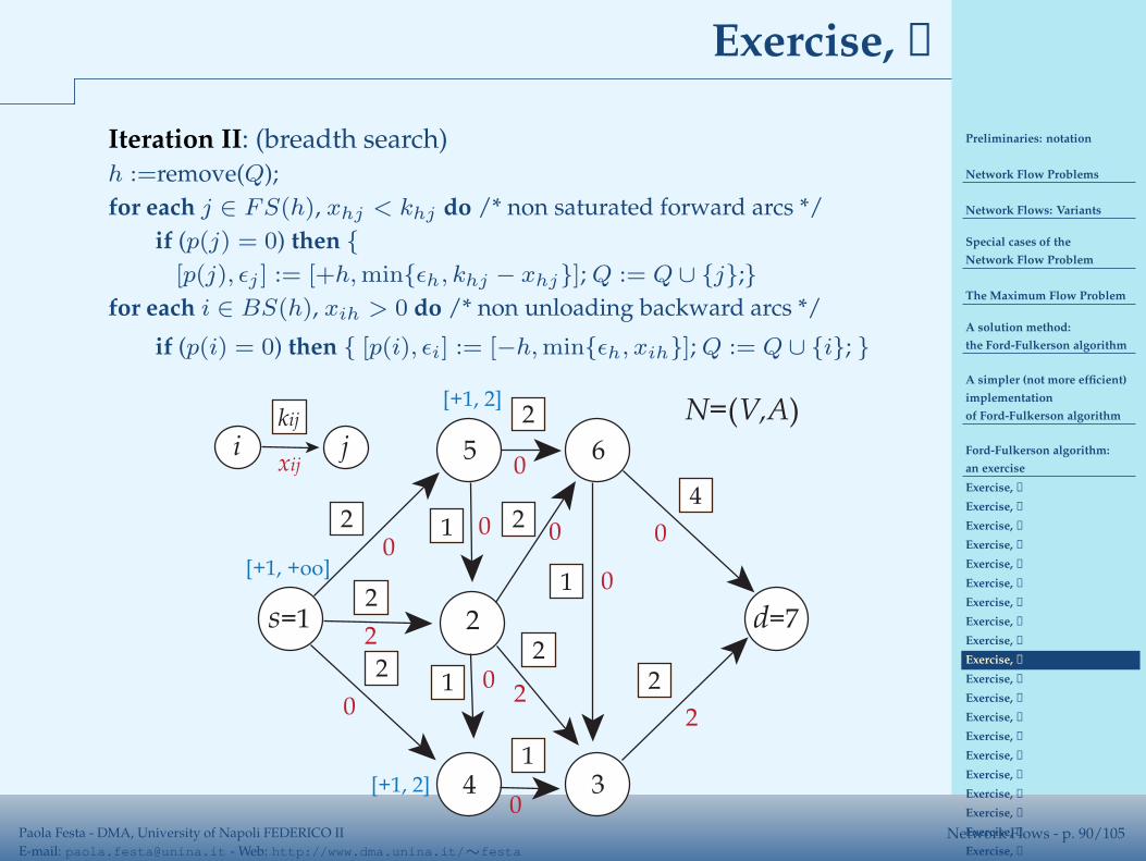
Preliminaries: notation
Network Flow Problems
Network Flows: Variants
Special cases of the
Network Flow Problem
The Maximum Flow Problem
A solution method:
the Ford-Fulkerson algorithm
A simpler (not more efficient)
implementation
of Ford-Fulkerson algorithm
Ford-Fulkerson algorithm:
an exercise
Exercise, ➀
Exercise, ➁
Exercise, ➂
Exercise, ➂
Exercise, ➂
Exercise, ➂
Exercise, ➂
Exercise, ➂
Exercise, ➂
Exercise, ➃
Exercise, ➃
Exercise, ➃
Exercise, ➃
Exercise, ➃
Exercise, ➃
Exercise, ➃
Exercise, ➃
Exercise, ➃
Exercise, ➃
Exercise, ➃
Exercise, ➄
Exercise, ➄
Paola Festa - DMA, University of Napoli FEDERICO II
E-mail: [email protected] - Web: http://www.dma.unina.it/∼festaNetwork Flows - p. 90/105
Exercise, ➃
Iteration II: (breadth search)h :=remove(Q);
for each j ∈ FS(h), xhj < khj do /* non saturated forward arcs */
if (p(j) = 0) then {
[p(j), ǫj ] := [+h, min{ǫh, khj − xhj}]; Q := Q ∪ {j};}
for each i ∈ BS(h), xih > 0 do /* non unloading backward arcs */
if (p(i) = 0) then { [p(i), ǫi] := [−h, min{ǫh, xih}]; Q := Q ∪ {i}; }
s=1
5
d=7
4
1
ikij
j 6
3
2
N=(V,A)
22
21
2
2
2
1
1
2
4
0
2
0
0
0
0
0
0
02
0
2
xij
[+1, +oo]
[+1, 2]
[+1, 2]
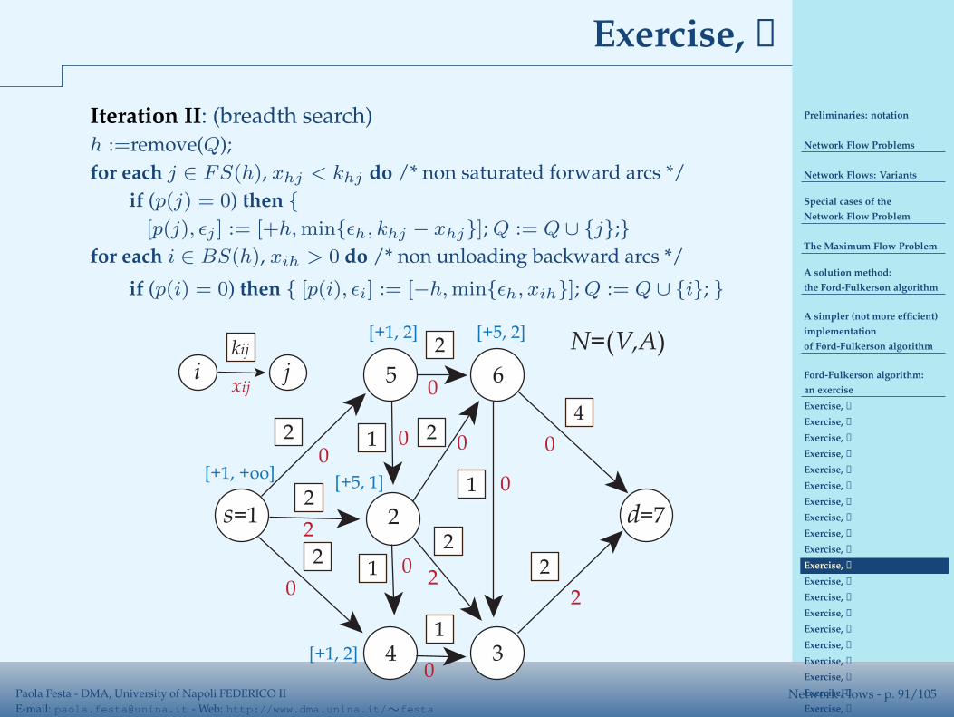
Preliminaries: notation
Network Flow Problems
Network Flows: Variants
Special cases of the
Network Flow Problem
The Maximum Flow Problem
A solution method:
the Ford-Fulkerson algorithm
A simpler (not more efficient)
implementation
of Ford-Fulkerson algorithm
Ford-Fulkerson algorithm:
an exercise
Exercise, ➀
Exercise, ➁
Exercise, ➂
Exercise, ➂
Exercise, ➂
Exercise, ➂
Exercise, ➂
Exercise, ➂
Exercise, ➂
Exercise, ➃
Exercise, ➃
Exercise, ➃
Exercise, ➃
Exercise, ➃
Exercise, ➃
Exercise, ➃
Exercise, ➃
Exercise, ➃
Exercise, ➃
Exercise, ➃
Exercise, ➄
Exercise, ➄
Paola Festa - DMA, University of Napoli FEDERICO II
E-mail: [email protected] - Web: http://www.dma.unina.it/∼festaNetwork Flows - p. 91/105
Exercise, ➃
Iteration II: (breadth search)h :=remove(Q);
for each j ∈ FS(h), xhj < khj do /* non saturated forward arcs */
if (p(j) = 0) then {
[p(j), ǫj ] := [+h, min{ǫh, khj − xhj}]; Q := Q ∪ {j};}
for each i ∈ BS(h), xih > 0 do /* non unloading backward arcs */
if (p(i) = 0) then { [p(i), ǫi] := [−h, min{ǫh, xih}]; Q := Q ∪ {i}; }
s=1
5
d=7
4
1
ikij
j 6
3
2
N=(V,A)
22
21
2
2
2
1
1
2
4
0
2
0
0
0
0
0
0
02
0
2
xij
[+1, +oo]
[+1, 2]
[+5, 1]
[+1, 2]
[+5, 2]
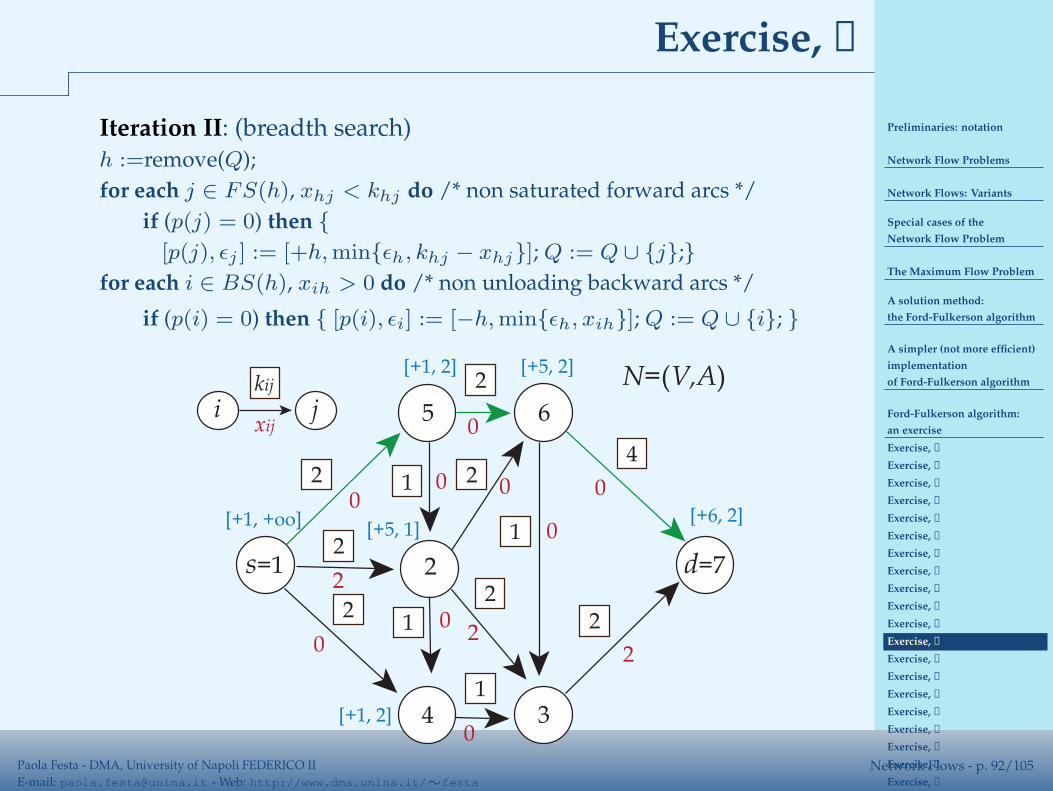
Preliminaries: notation
Network Flow Problems
Network Flows: Variants
Special cases of the
Network Flow Problem
The Maximum Flow Problem
A solution method:
the Ford-Fulkerson algorithm
A simpler (not more efficient)
implementation
of Ford-Fulkerson algorithm
Ford-Fulkerson algorithm:
an exercise
Exercise, ➀
Exercise, ➁
Exercise, ➂
Exercise, ➂
Exercise, ➂
Exercise, ➂
Exercise, ➂
Exercise, ➂
Exercise, ➂
Exercise, ➃
Exercise, ➃
Exercise, ➃
Exercise, ➃
Exercise, ➃
Exercise, ➃
Exercise, ➃
Exercise, ➃
Exercise, ➃
Exercise, ➃
Exercise, ➃
Exercise, ➄
Exercise, ➄
Paola Festa - DMA, University of Napoli FEDERICO II
E-mail: [email protected] - Web: http://www.dma.unina.it/∼festaNetwork Flows - p. 92/105
Exercise, ➃
Iteration II: (breadth search)h :=remove(Q);
for each j ∈ FS(h), xhj < khj do /* non saturated forward arcs */
if (p(j) = 0) then {
[p(j), ǫj ] := [+h, min{ǫh, khj − xhj}]; Q := Q ∪ {j};}
for each i ∈ BS(h), xih > 0 do /* non unloading backward arcs */
if (p(i) = 0) then { [p(i), ǫi] := [−h, min{ǫh, xih}]; Q := Q ∪ {i}; }
s=1
5
d=7
4
1
ikij
j 6
3
2
N=(V,A)
22
21
2
2
2
1
1
2
4
0
2
0
0
0
0
0
0
02
0
2
xij
[+1, +oo]
[+1, 2]
[+5, 1]
[+1, 2]
[+5, 2]
[+6, 2]
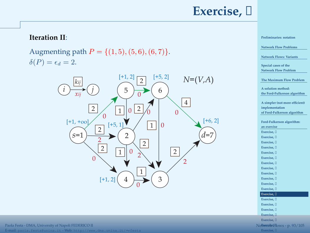
Preliminaries: notation
Network Flow Problems
Network Flows: Variants
Special cases of the
Network Flow Problem
The Maximum Flow Problem
A solution method:
the Ford-Fulkerson algorithm
A simpler (not more efficient)
implementation
of Ford-Fulkerson algorithm
Ford-Fulkerson algorithm:
an exercise
Exercise, ➀
Exercise, ➁
Exercise, ➂
Exercise, ➂
Exercise, ➂
Exercise, ➂
Exercise, ➂
Exercise, ➂
Exercise, ➂
Exercise, ➃
Exercise, ➃
Exercise, ➃
Exercise, ➃
Exercise, ➃
Exercise, ➃
Exercise, ➃
Exercise, ➃
Exercise, ➃
Exercise, ➃
Exercise, ➃
Exercise, ➄
Exercise, ➄
Paola Festa - DMA, University of Napoli FEDERICO II
E-mail: [email protected] - Web: http://www.dma.unina.it/∼festaNetwork Flows - p. 93/105
Exercise, ➃
Iteration II:
Augmenting path P = {(1, 5), (5, 6), (6, 7)}.
δ(P ) = ǫd = 2.
s=1
5
d=7
4
1
ikij
j 6
3
2
N=(V,A)
22
21
2
2
2
1
1
2
4
0
2
0
0
0
0
0
0
02
0
2
xij
[+1, +oo]
[+1, 2]
[+5, 1]
[+1, 2]
[+5, 2]
[+6, 2]
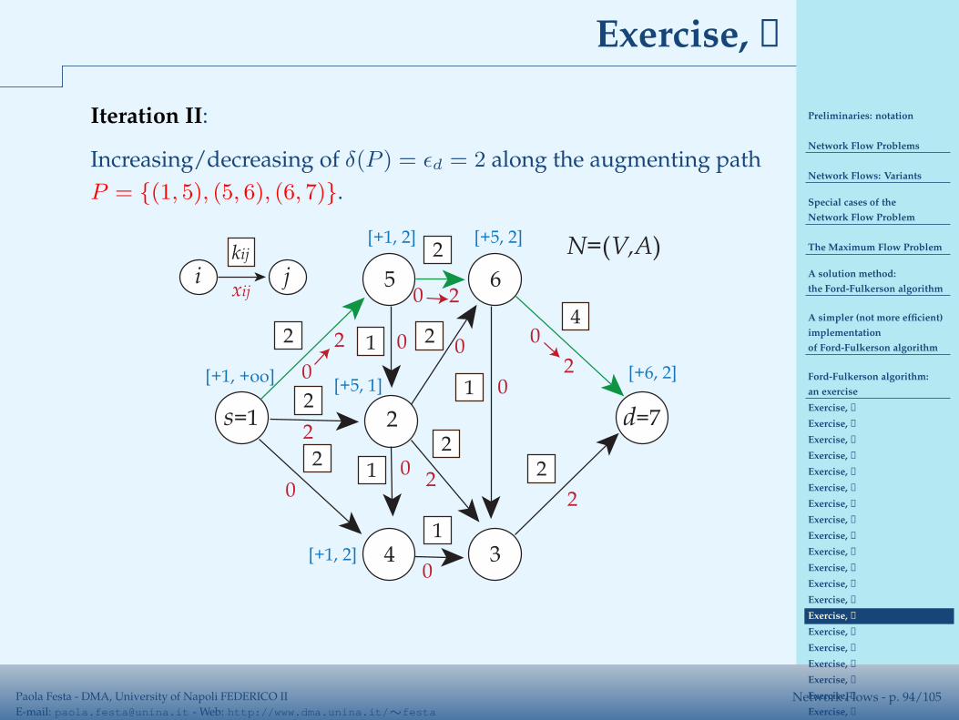
Preliminaries: notation
Network Flow Problems
Network Flows: Variants
Special cases of the
Network Flow Problem
The Maximum Flow Problem
A solution method:
the Ford-Fulkerson algorithm
A simpler (not more efficient)
implementation
of Ford-Fulkerson algorithm
Ford-Fulkerson algorithm:
an exercise
Exercise, ➀
Exercise, ➁
Exercise, ➂
Exercise, ➂
Exercise, ➂
Exercise, ➂
Exercise, ➂
Exercise, ➂
Exercise, ➂
Exercise, ➃
Exercise, ➃
Exercise, ➃
Exercise, ➃
Exercise, ➃
Exercise, ➃
Exercise, ➃
Exercise, ➃
Exercise, ➃
Exercise, ➃
Exercise, ➃
Exercise, ➄
Exercise, ➄
Paola Festa - DMA, University of Napoli FEDERICO II
E-mail: [email protected] - Web: http://www.dma.unina.it/∼festaNetwork Flows - p. 94/105
Exercise, ➃
Iteration II:
Increasing/decreasing of δ(P ) = ǫd = 2 along the augmenting path
P = {(1, 5), (5, 6), (6, 7)}.
s=1
5
d=7
4
1
ikij
j 6
3
2
N=(V,A)
22
21
2
2
2
1
1
2
4
0
2
0
0
0
0
0
0
02
0
2
xij
[+1, +oo]
[+1, 2]
[+5, 1]
[+1, 2]
[+5, 2]
[+6, 2]
2
2
2

Preliminaries: notation
Network Flow Problems
Network Flows: Variants
Special cases of the
Network Flow Problem
The Maximum Flow Problem
A solution method:
the Ford-Fulkerson algorithm
A simpler (not more efficient)
implementation
of Ford-Fulkerson algorithm
Ford-Fulkerson algorithm:
an exercise
Exercise, ➀
Exercise, ➁
Exercise, ➂
Exercise, ➂
Exercise, ➂
Exercise, ➂
Exercise, ➂
Exercise, ➂
Exercise, ➂
Exercise, ➃
Exercise, ➃
Exercise, ➃
Exercise, ➃
Exercise, ➃
Exercise, ➃
Exercise, ➃
Exercise, ➃
Exercise, ➃
Exercise, ➃
Exercise, ➃
Exercise, ➄
Exercise, ➄
Paola Festa - DMA, University of Napoli FEDERICO II
E-mail: [email protected] - Web: http://www.dma.unina.it/∼festaNetwork Flows - p. 95/105
Exercise, ➃
End of Iteration II:
ϕ0 = 4.
s=1
5
d=7
4
1
ikij
j 6
3
2
N=(V,A)
22
21
2
2
2
1
1
2
4
2
2
0
0
2
0
0
2
02
0
2
xij
[+1, +oo]
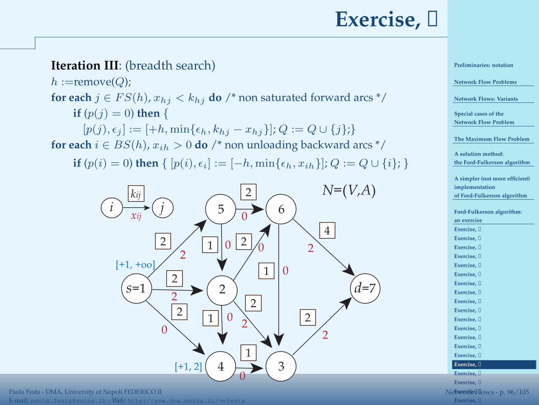
Preliminaries: notation
Network Flow Problems
Network Flows: Variants
Special cases of the
Network Flow Problem
The Maximum Flow Problem
A solution method:
the Ford-Fulkerson algorithm
A simpler (not more efficient)
implementation
of Ford-Fulkerson algorithm
Ford-Fulkerson algorithm:
an exercise
Exercise, ➀
Exercise, ➁
Exercise, ➂
Exercise, ➂
Exercise, ➂
Exercise, ➂
Exercise, ➂
Exercise, ➂
Exercise, ➂
Exercise, ➃
Exercise, ➃
Exercise, ➃
Exercise, ➃
Exercise, ➃
Exercise, ➃
Exercise, ➃
Exercise, ➃
Exercise, ➃
Exercise, ➃
Exercise, ➃
Exercise, ➄
Exercise, ➄
Paola Festa - DMA, University of Napoli FEDERICO II
E-mail: [email protected] - Web: http://www.dma.unina.it/∼festaNetwork Flows - p. 96/105
Exercise, ➃
Iteration III: (breadth search)h :=remove(Q);
for each j ∈ FS(h), xhj < khj do /* non saturated forward arcs */
if (p(j) = 0) then {
[p(j), ǫj ] := [+h, min{ǫh, khj − xhj}]; Q := Q ∪ {j};}
for each i ∈ BS(h), xih > 0 do /* non unloading backward arcs */
if (p(i) = 0) then { [p(i), ǫi] := [−h, min{ǫh, xih}]; Q := Q ∪ {i}; }
s=1
5
d=7
4
1
ikij
j 6
3
2
N=(V,A)
22
21
2
2
2
1
1
2
4
2
2
0
0
0
0
0
2
02
0
2
xij
[+1, +oo]
[+1, 2]

Preliminaries: notation
Network Flow Problems
Network Flows: Variants
Special cases of the
Network Flow Problem
The Maximum Flow Problem
A solution method:
the Ford-Fulkerson algorithm
A simpler (not more efficient)
implementation
of Ford-Fulkerson algorithm
Ford-Fulkerson algorithm:
an exercise
Exercise, ➀
Exercise, ➁
Exercise, ➂
Exercise, ➂
Exercise, ➂
Exercise, ➂
Exercise, ➂
Exercise, ➂
Exercise, ➂
Exercise, ➃
Exercise, ➃
Exercise, ➃
Exercise, ➃
Exercise, ➃
Exercise, ➃
Exercise, ➃
Exercise, ➃
Exercise, ➃
Exercise, ➃
Exercise, ➃
Exercise, ➄
Exercise, ➄
Paola Festa - DMA, University of Napoli FEDERICO II
E-mail: [email protected] - Web: http://www.dma.unina.it/∼festaNetwork Flows - p. 97/105
Exercise, ➃
Iteration III: (breadth search)h :=remove(Q);
for each j ∈ FS(h), xhj < khj do /* non saturated forward arcs */
if (p(j) = 0) then {
[p(j), ǫj ] := [+h, min{ǫh, khj − xhj}]; Q := Q ∪ {j};}
for each i ∈ BS(h), xih > 0 do /* non unloading backward arcs */
if (p(i) = 0) then { [p(i), ǫi] := [−h, min{ǫh, xih}]; Q := Q ∪ {i}; }
s=1
5
d=7
4
1
ikij
j 6
3
2
N=(V,A)
22
21
2
2
2
1
1
2
4
2
2
0
0
0
0
0
2
02
0
2
xij
[+1, +oo]
[+1, 2] [+4, 1]
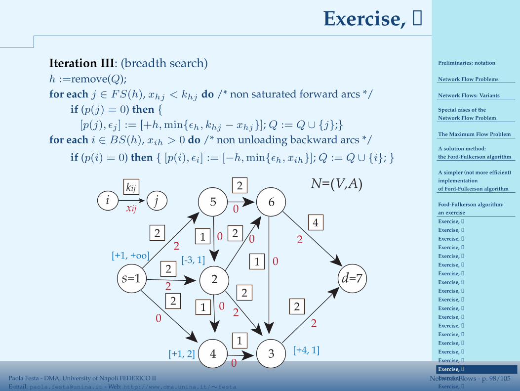
Preliminaries: notation
Network Flow Problems
Network Flows: Variants
Special cases of the
Network Flow Problem
The Maximum Flow Problem
A solution method:
the Ford-Fulkerson algorithm
A simpler (not more efficient)
implementation
of Ford-Fulkerson algorithm
Ford-Fulkerson algorithm:
an exercise
Exercise, ➀
Exercise, ➁
Exercise, ➂
Exercise, ➂
Exercise, ➂
Exercise, ➂
Exercise, ➂
Exercise, ➂
Exercise, ➂
Exercise, ➃
Exercise, ➃
Exercise, ➃
Exercise, ➃
Exercise, ➃
Exercise, ➃
Exercise, ➃
Exercise, ➃
Exercise, ➃
Exercise, ➃
Exercise, ➃
Exercise, ➄
Exercise, ➄
Paola Festa - DMA, University of Napoli FEDERICO II
E-mail: [email protected] - Web: http://www.dma.unina.it/∼festaNetwork Flows - p. 98/105
Exercise, ➃
Iteration III: (breadth search)h :=remove(Q);
for each j ∈ FS(h), xhj < khj do /* non saturated forward arcs */
if (p(j) = 0) then {
[p(j), ǫj ] := [+h, min{ǫh, khj − xhj}]; Q := Q ∪ {j};}
for each i ∈ BS(h), xih > 0 do /* non unloading backward arcs */
if (p(i) = 0) then { [p(i), ǫi] := [−h, min{ǫh, xih}]; Q := Q ∪ {i}; }
s=1
5
d=7
4
1
ikij
j 6
3
2
N=(V,A)
22
21
2
2
2
1
1
2
4
2
2
0
0
0
0
0
2
02
0
2
xij
[+1, +oo]
[+1, 2] [+4, 1]
[-3, 1]

Preliminaries: notation
Network Flow Problems
Network Flows: Variants
Special cases of the
Network Flow Problem
The Maximum Flow Problem
A solution method:
the Ford-Fulkerson algorithm
A simpler (not more efficient)
implementation
of Ford-Fulkerson algorithm
Ford-Fulkerson algorithm:
an exercise
Exercise, ➀
Exercise, ➁
Exercise, ➂
Exercise, ➂
Exercise, ➂
Exercise, ➂
Exercise, ➂
Exercise, ➂
Exercise, ➂
Exercise, ➃
Exercise, ➃
Exercise, ➃
Exercise, ➃
Exercise, ➃
Exercise, ➃
Exercise, ➃
Exercise, ➃
Exercise, ➃
Exercise, ➃
Exercise, ➃
Exercise, ➄
Exercise, ➄
Paola Festa - DMA, University of Napoli FEDERICO II
E-mail: [email protected] - Web: http://www.dma.unina.it/∼festaNetwork Flows - p. 99/105
Exercise, ➃
Iteration III: (breadth search)h :=remove(Q);
for each j ∈ FS(h), xhj < khj do /* non saturated forward arcs */
if (p(j) = 0) then {
[p(j), ǫj ] := [+h, min{ǫh, khj − xhj}]; Q := Q ∪ {j};}
for each i ∈ BS(h), xih > 0 do /* non unloading backward arcs */
if (p(i) = 0) then { [p(i), ǫi] := [−h, min{ǫh, xih}]; Q := Q ∪ {i}; }
s=1
5
d=7
4
1
ikij
j 6
3
2
N=(V,A)
22
21
2
2
2
1
1
2
4
2
2
0
0
0
0
0
2
02
0
2
xij
[+1, +oo]
[+1, 2] [+4, 1]
[-3, 1]
[+2, 1]
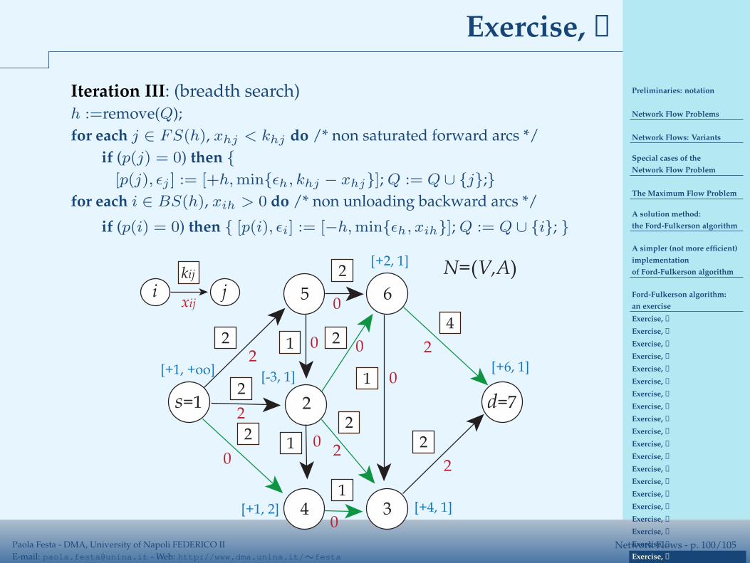
Preliminaries: notation
Network Flow Problems
Network Flows: Variants
Special cases of the
Network Flow Problem
The Maximum Flow Problem
A solution method:
the Ford-Fulkerson algorithm
A simpler (not more efficient)
implementation
of Ford-Fulkerson algorithm
Ford-Fulkerson algorithm:
an exercise
Exercise, ➀
Exercise, ➁
Exercise, ➂
Exercise, ➂
Exercise, ➂
Exercise, ➂
Exercise, ➂
Exercise, ➂
Exercise, ➂
Exercise, ➃
Exercise, ➃
Exercise, ➃
Exercise, ➃
Exercise, ➃
Exercise, ➃
Exercise, ➃
Exercise, ➃
Exercise, ➃
Exercise, ➃
Exercise, ➃
Exercise, ➄
Exercise, ➄
Paola Festa - DMA, University of Napoli FEDERICO II
E-mail: [email protected] - Web: http://www.dma.unina.it/∼festaNetwork Flows - p. 100/105
Exercise, ➃
Iteration III: (breadth search)h :=remove(Q);
for each j ∈ FS(h), xhj < khj do /* non saturated forward arcs */
if (p(j) = 0) then {
[p(j), ǫj ] := [+h, min{ǫh, khj − xhj}]; Q := Q ∪ {j};}
for each i ∈ BS(h), xih > 0 do /* non unloading backward arcs */
if (p(i) = 0) then { [p(i), ǫi] := [−h, min{ǫh, xih}]; Q := Q ∪ {i}; }
s=1
5
d=7
4
1
ikij
j 6
3
2
N=(V,A)
22
21
2
2
2
1
1
2
4
2
2
0
0
0
0
0
2
02
0
2
xij
[+1, +oo][-3, 1]
[+1, 2]
[+2, 1]
[+6, 1]
[+4, 1]
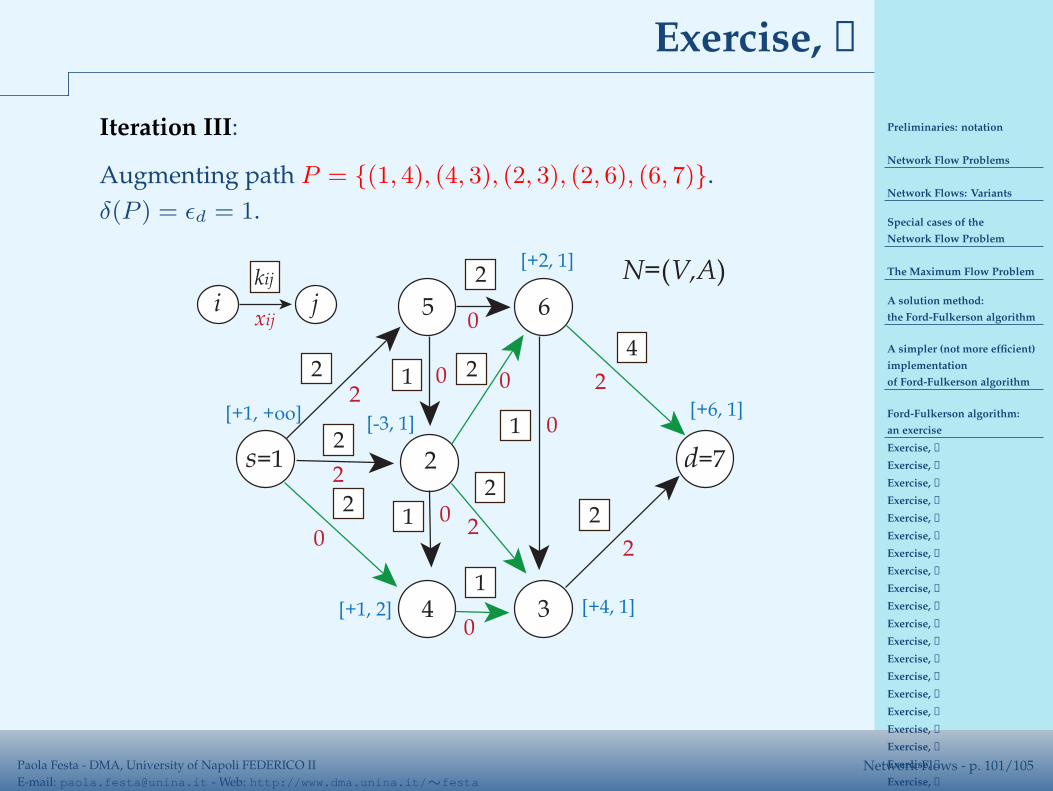
Preliminaries: notation
Network Flow Problems
Network Flows: Variants
Special cases of the
Network Flow Problem
The Maximum Flow Problem
A solution method:
the Ford-Fulkerson algorithm
A simpler (not more efficient)
implementation
of Ford-Fulkerson algorithm
Ford-Fulkerson algorithm:
an exercise
Exercise, ➀
Exercise, ➁
Exercise, ➂
Exercise, ➂
Exercise, ➂
Exercise, ➂
Exercise, ➂
Exercise, ➂
Exercise, ➂
Exercise, ➃
Exercise, ➃
Exercise, ➃
Exercise, ➃
Exercise, ➃
Exercise, ➃
Exercise, ➃
Exercise, ➃
Exercise, ➃
Exercise, ➃
Exercise, ➃
Exercise, ➄
Exercise, ➄
Paola Festa - DMA, University of Napoli FEDERICO II
E-mail: [email protected] - Web: http://www.dma.unina.it/∼festaNetwork Flows - p. 101/105
Exercise, ➄
Iteration III:
Augmenting path P = {(1, 4), (4, 3), (2, 3), (2, 6), (6, 7)}.
δ(P ) = ǫd = 1.
s=1
5
d=7
4
1
ikij
j 6
3
2
N=(V,A)
22
21
2
2
2
1
1
2
4
2
2
0
0
0
0
0
2
02
0
2
xij
[+1, +oo][-3, 1]
[+1, 2]
[+2, 1]
[+6, 1]
[+4, 1]
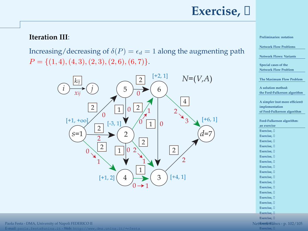
Preliminaries: notation
Network Flow Problems
Network Flows: Variants
Special cases of the
Network Flow Problem
The Maximum Flow Problem
A solution method:
the Ford-Fulkerson algorithm
A simpler (not more efficient)
implementation
of Ford-Fulkerson algorithm
Ford-Fulkerson algorithm:
an exercise
Exercise, ➀
Exercise, ➁
Exercise, ➂
Exercise, ➂
Exercise, ➂
Exercise, ➂
Exercise, ➂
Exercise, ➂
Exercise, ➂
Exercise, ➃
Exercise, ➃
Exercise, ➃
Exercise, ➃
Exercise, ➃
Exercise, ➃
Exercise, ➃
Exercise, ➃
Exercise, ➃
Exercise, ➃
Exercise, ➃
Exercise, ➄
Exercise, ➄
Paola Festa - DMA, University of Napoli FEDERICO II
E-mail: [email protected] - Web: http://www.dma.unina.it/∼festaNetwork Flows - p. 102/105
Exercise, ➄
Iteration III:
Increasing/decreasing of δ(P ) = ǫd = 1 along the augmenting path
P = {(1, 4), (4, 3), (2, 3), (2, 6), (6, 7)}.
s=1
5
d=7
4
1
ikij
j 6
3
2
N=(V,A)
22
21
2
2
2
1
1
2
4
0
2
0
0
0
0 0
2
0 2
0
2
xij
[+1, +oo][-3, 1]
[+1, 2]
[+2, 1]
[+6, 1]
[+4, 1]
1
1
3
1
1
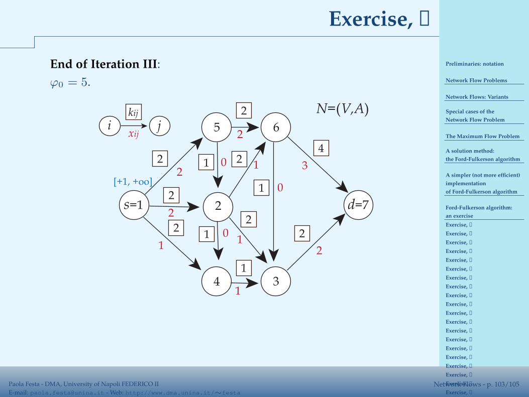
Preliminaries: notation
Network Flow Problems
Network Flows: Variants
Special cases of the
Network Flow Problem
The Maximum Flow Problem
A solution method:
the Ford-Fulkerson algorithm
A simpler (not more efficient)
implementation
of Ford-Fulkerson algorithm
Ford-Fulkerson algorithm:
an exercise
Exercise, ➀
Exercise, ➁
Exercise, ➂
Exercise, ➂
Exercise, ➂
Exercise, ➂
Exercise, ➂
Exercise, ➂
Exercise, ➂
Exercise, ➃
Exercise, ➃
Exercise, ➃
Exercise, ➃
Exercise, ➃
Exercise, ➃
Exercise, ➃
Exercise, ➃
Exercise, ➃
Exercise, ➃
Exercise, ➃
Exercise, ➄
Exercise, ➄
Paola Festa - DMA, University of Napoli FEDERICO II
E-mail: [email protected] - Web: http://www.dma.unina.it/∼festaNetwork Flows - p. 103/105
Exercise, ➄
End of Iteration III:
ϕ0 = 5.
s=1
5
d=7
4
1
ikij
j 6
3
2
N=(V,A)
22
21
2
2
2
1
1
2
4
2
2
1
0
2
1
0
3
01
1
2
xij
[+1, +oo]
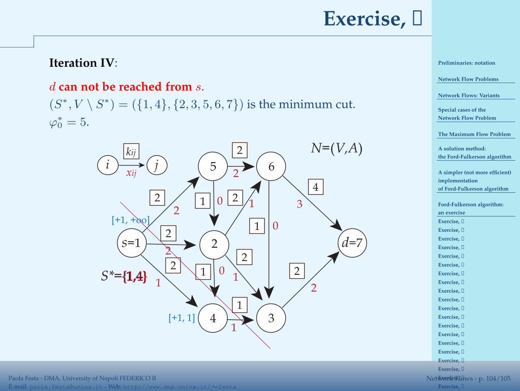
Preliminaries: notation
Network Flow Problems
Network Flows: Variants
Special cases of the
Network Flow Problem
The Maximum Flow Problem
A solution method:
the Ford-Fulkerson algorithm
A simpler (not more efficient)
implementation
of Ford-Fulkerson algorithm
Ford-Fulkerson algorithm:
an exercise
Exercise, ➀
Exercise, ➁
Exercise, ➂
Exercise, ➂
Exercise, ➂
Exercise, ➂
Exercise, ➂
Exercise, ➂
Exercise, ➂
Exercise, ➃
Exercise, ➃
Exercise, ➃
Exercise, ➃
Exercise, ➃
Exercise, ➃
Exercise, ➃
Exercise, ➃
Exercise, ➃
Exercise, ➃
Exercise, ➃
Exercise, ➄
Exercise, ➄
Paola Festa - DMA, University of Napoli FEDERICO II
E-mail: [email protected] - Web: http://www.dma.unina.it/∼festaNetwork Flows - p. 104/105
Exercise, ➅
Iteration IV:
d can not be reached from s.
(S∗, V \ S∗) = ({1, 4}, {2, 3, 5, 6, 7}) is the minimum cut.
ϕ∗0 = 5.
s=1
5
d=7
4
1
ikij
j 6
3
2
N=(V,A)
22
21
2
2
2
1
1
2
4
2
2
1
0
2
1
0
3
01
1
2
xij
[+1, +oo]
[+1, 1]
S*={1,4}
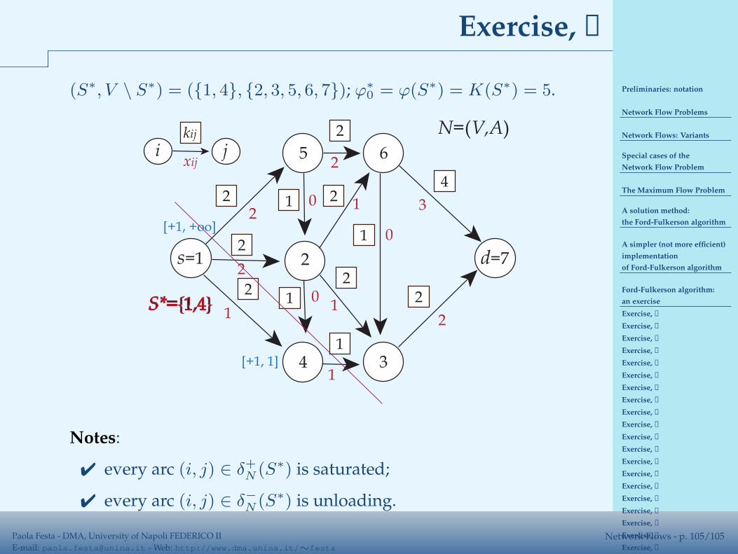
Preliminaries: notation
Network Flow Problems
Network Flows: Variants
Special cases of the
Network Flow Problem
The Maximum Flow Problem
A solution method:
the Ford-Fulkerson algorithm
A simpler (not more efficient)
implementation
of Ford-Fulkerson algorithm
Ford-Fulkerson algorithm:
an exercise
Exercise, ➀
Exercise, ➁
Exercise, ➂
Exercise, ➂
Exercise, ➂
Exercise, ➂
Exercise, ➂
Exercise, ➂
Exercise, ➂
Exercise, ➃
Exercise, ➃
Exercise, ➃
Exercise, ➃
Exercise, ➃
Exercise, ➃
Exercise, ➃
Exercise, ➃
Exercise, ➃
Exercise, ➃
Exercise, ➃
Exercise, ➄
Exercise, ➄
Paola Festa - DMA, University of Napoli FEDERICO II
E-mail: [email protected] - Web: http://www.dma.unina.it/∼festaNetwork Flows - p. 105/105
Exercise, ➆
(S∗, V \ S∗) = ({1, 4}, {2, 3, 5, 6, 7}); ϕ∗0 = ϕ(S∗) = K(S∗) = 5.
s=1
5
d=7
4
1
ikij
j 6
3
2
N=(V,A)
22
21
2
2
2
1
1
2
4
2
2
1
0
2
1
0
3
01
1
2
xij
[+1, +oo]
[+1, 1]
S*={1,4}
Notes:
✔ every arc (i, j) ∈ δ+N (S∗) is saturated;
✔ every arc (i, j) ∈ δ−N (S∗) is unloading.