Prepared by Alan Guthrie, Michael Hartley, Alex Moon… · Redesigning the ME 331 Heat Conduction Experiment Prepared by Alan Guthrie, Michael Hartley, Alex Moon, and Krista Simonson

Redesigning the ME 331 Heat Conduction Experiment

Prepared by Alan Guthrie, Michael Hartley,

Alex Moon, and Krista Simonson

Group E

Prepared for Mr. Shazib Vijlee, Mechanical Engineering PhD Student

University of Washington

June 2012

ii

EXECUTIVE SUMMARY This report provides a detailed discussion of the work completed by Group E in designing and manufacturing a new heat conduction lab experiment for the ME 331 Heat Transfer class at the University of Washington. The objective of this project is to design and test this lab experiment that will test students’ understanding of heat transfer by conduction, while producing consistent, accurate, and measurable results. The final concept design that was selected is a cylindrical setup, where students are required to measure the temperature difference across the radius of a cylindrical specimen. The lab prototype consists of a heating rod, wrapped in the material to be tested and suspended in the air with support blocks, made out of Temperlite insulation, on each end of the rod. The power is controlled by a variac, which regulates the voltage received by the heating rod. Data acquisition is performed with thermocouples attached to the inner and outer surfaces of the specimen in coordination with Personal Daq View software. The specimen being tested is ultra-flexible foam rubber pipe insulation with a literature thermal conductivity value of 0.036 W/m-K. There is also a lab handout that will be handed to the students that instructs them on how to collect the data and analyze it, testing their ability to apply the conduction equation to a radial system. Additionally, a COMSOL pre-lab activity was designed to enhance the students’ lab experience. This design is a significant improvement to the conduction lab experiment currently in use by the ME 331 Heat Transfer class instructors. The current system consistently gives students a large percent error between measured and theoretical values. This new cylindrical design eliminates much of the error due to multidimensionality that was present in the old lab, and consistently produces results with a percent error of 10-15% for the calculated thermal conductivity. The system is simple to operate, and the designed lab handout adequately tests the students’ understanding of the fundamental concepts surrounding heat conduction. The design is not as interesting or as complex as multi-layered systems, but it produces accurate, consistent results. If approved by the client and future instructors of the ME 331 Heat Transfer class, this lab experiment could easily be incorporated into the class curriculum. It would make an excellent addition to the course and would give students’ an opportunity to physically apply the concepts they are being taught in the classroom.

iii

TABLE OF CONTENTS LIST OF FIGURES .............................................................................................................. v

LIST OF TABLES ................................................................................................................ v INTRODUCTION ................................................................................................................. 1

Background ..................................................................................................................................... 1 Purpose ............................................................................................................................................ 1

DESIGN PROBLEM DEFINITION ................................................................................... 2

CURRENT TECHNOLOGY ............................................................................................... 3 CONCEPT GENERATION, EVALUATION, AND SELECTION ................................. 4

Overall Setup of New Lab .............................................................................................................. 4 Box Setup ..................................................................................................................................... 5 Cylindrical Setup .......................................................................................................................... 5

Determining Material ..................................................................................................................... 6 Large Temperature Gradient ........................................................................................................ 6 Steady-State Arrival Time ............................................................................................................ 7 Availability and Machinability of Cylindrical Specimen ............................................................. 7

Multi-Layered System .................................................................................................................... 7 In-Lab Experiment and Post-Lab Write-Up ................................................................................ 8

Single Cylindrical Setup ............................................................................................................... 8 Compare Two Cylindrical Setups with Different Materials ......................................................... 8 Old vs. New Setup and Comparing Results for Same Material ................................................... 8

COMSOL Pre-Lab Activity ........................................................................................................... 9 FINAL CONCEPTUAL DESIGN ....................................................................................... 9

General Description ........................................................................................................................ 9 Components ................................................................................................................................... 10

Heating Rod ................................................................................................................................ 10 Design .................................................................................................................................................... 10 Advantages/Disadvantages .................................................................................................................... 11

Ultra-Flexible Foam Rubber Pipe Insulation .............................................................................. 11 Design .................................................................................................................................................... 11 Advantages/Disadvantages .................................................................................................................... 11

Thermocouples ........................................................................................................................... 12 Design .................................................................................................................................................... 12 Advantages/Disadvantages .................................................................................................................... 12

Temperlite Blocks ....................................................................................................................... 13 Design .................................................................................................................................................... 13 Advantages/Disadvantages .................................................................................................................... 13

Data Acquisition Setup and Power Supply ................................................................................. 13 Design .................................................................................................................................................... 13 Advantages/Disadvantages .................................................................................................................... 14

Lab Handout 1: Old vs. New Setup and Comparing Results for Same Material ....................... 14 Lab Handout 2: Single Cylindrical Setup ................................................................................... 14 COMSOL Pre-Lab Activity ........................................................................................................ 15

DETAILED DESIGN, PROTOTYPE MANUFACTURE AND EVALUATION ........ 15 MODELING AND ANALYSIS ......................................................................................... 16

ECONOMIC/COST EVALUATION ................................................................................ 19

iv

CONSIDERATION OF THE BROADER CONTEXT OF DESIGN ............................ 20 Risk and Liability ......................................................................................................................... 20 Ethical Issues/Societal Impact ..................................................................................................... 20 Impact on Environment ............................................................................................................... 20

FUTURE WORK ................................................................................................................ 20 REFERENCES .................................................................................................................... 22

APPENDIX A: LAB HANDOUT FOR CURRENT CONDUCTION LAB .................. 23 APPENDIX B: MATLAB CODE ...................................................................................... 26

APPENDIX C: LAB HANDOUT INCORPORATING RECTANGULAR AND CYLINDRICAL CONDUCTION LABS .......................................................................... 27

APPENDIX D: LAB HANDOUT FOR THE CYLINDRICAL CONDUCTION LAB 31 APPENDIX E: COMSOL PRE-LAB ACTIVITY ........................................................... 34

APPENDIX F: TESTING RESULTS ............................................................................... 41

v

LIST OF FIGURES Figure 1. Current Conduction Lab Setup .......................................................................... 4

Figure 2. Schematic for the Current Conduction Lab ...................................................... 5 Figure 3. Final Setup of the Redesigned Lab .................................................................... 10

Figure 4. Cylindrical Heating Rod with Tape .................................................................. 10 Figure 5. Cross Sectional View of the Foam Rubber Pipe Insulation ............................ 11

Figure 6. Placement of Thermocouples along Heating Rod ............................................ 12 Figure 7. Placement of Thermocouples along Outside of Insulation .............................. 12

Figure 8. Temperlite Block ................................................................................................. 13 Figure 9. Power Supply System ......................................................................................... 14

Figure 10. COMSOL Simulation of the Cylindrical Model ............................................ 15 Figure 11. May 22, 2012 Test of Foam Rubber: k vs. Distance From End of Specimen ............................................................................................................................................... 18 Figure 12. Range of Thermal Conductivities for Silicone Foams .................................. 19

LIST OF TABLES Table I. Pugh Chart Comparing Characteristics of Different Materials ........................ 6 Table II. May 22, 2012 Test Results for Foam Rubber Insulation ................................. 17

Table F1. May 10 Testing Results ...................................................................................... 41 Table F2. May 11 Testing Results ...................................................................................... 41




1

INTRODUCTION Background Mechanical Engineering students at the University of Washington are required by ABET standards to complete a heat transfer class in order to obtain their Bachelor’s degree. This course covers the conduction and convection modes of heat transfer with experiments. Due to extreme experimental error, arising in no small part from incorrect assumptions about the directionality of heat transfer, the laboratory experiment for conduction must be remade. Our client Shazib Vijlee, a graduate student in the Mechanical Engineering department, believes that the error can be mostly eliminated by switching from a rectangular model to a cylindrical one. Conduction is the transfer of heat through solid surfaces. It is governed by the conduction equation, which relates heat flow to the temperature gradient present, the physical dimensions of the solid, and the thermal conductivity of the material. For uniaxial heat flow, the equation takes the form 𝑞 = −𝑘𝐴 !"

!" , where q is equal to heat flow measured in Watts, k is the thermal

conductivity measured in W/m-K, A is the cross sectional area measured in m2, and dT/dx is the change in temperature across the length of the specimen. Heat is always transferred in the direction of decreasing temperature. The application of the conduction equation to a cylindrical system is as follows:

𝑞 =2𝜋𝐿𝑘 𝑇!! − 𝑇!!

ln 𝑟! 𝑟!

L is the length of the cylinder measured in meters, Ts1 is the temperature of the inner surface measured in Kelvin, Ts2 is the temperature of the outer surface measured in Kelvin, r1 is the inner radius in meters, and r2 is the outer radius in meters. This allows one to calculate the heat flow in the radial direction of a cylindrical specimen, and it is the equation that was applied throughout or design and evaluation of or product. [1] Purpose The University of Washington’s Mechanical Engineering Program requires all undergraduates to complete the fundamental curricula in order to obtain a bachelor’s degree. Of these fundamental curricula, the ME 331 course introduces students to the study of heat transfer by conduction, convection, and radiation. The current course is taught by Professor Emery, who also oversees the coursework, and is assisted by Shazib Vijlee. Sponsored by Professor Emery, Shazib Vijlee has presented an opportunity to redesign the current ME 331 heat conduction lab exercise to having a working lab that can provide accurate results as well as improve students’ connection to the theory taught in class. The objective of this project is to design and test such a lab experiment that will test students’ understanding of heat transfer by conduction, while producing consistent, accurate, and measurable results.

2

DESIGN PROBLEM DEFINITION The main objective of this project is to design and build a new conductive heat transfer experiment for the ME 331 Heat Transfer class. The purpose of the new setup is to further enforce the heat conduction theory through a physical model in which information can be analyzed. Through the communication with our client, Shazib, we have established a list of functional requirements that our client would like to be addressed through our project. Below, these requirements have been ranked by the manner of importance:

1. Students should be able to match analysis of the experiment with a theory learned in class.

2. The experiment must be safe, meaning it won’t catch fire and the external surface won’t be so hot that it would cause serious injury to students who touched it.

3. Reduce heat flow in unwanted directions. 4. Experiment setup takes approximately 30 minutes to reach steady state. 5. Experiment is capable of measuring desired parameters. 6. Have working data acquisition system that provides accurate data. 7. Temperature must be measured at a minimum of two locations along in the desired

direction of conductive heat flow (at the heater-material interface and the external surface of the material), but the more temperature measuring locations the better.

8. Choose materials so that there is a large change of temperature observed during the experiment.

9. Write up a lab exercise with an answer key showing the expected results. 10. Use of COMSOL in the lab exercise. Students should model what they experienced in lab

and possibly model other materials unable to be tested in this lab setting. 11. Make experiment as “visual” as possible.

We realized that our client had given us two goals that are compliant with these functional requirements; a realistic goal and an aggressive goal. The client’s realistic goal is that we design and build a conductive heat transfer experiment but the aggressive goal is that along with building a conductive heat transfer experiment, we test and create a working lab exercise with an answer key. With this, our group has went along with completing the client’s aggressive goal. However, with this in mind, there are constraints associated with this project that may limit our ideas. Our design constraints are fairly straightforward and simple. First of all, the design must be safe. The operating temperature of the model must be at a level that would not cause any materials to catch fire or cause any harm to students. In addition, the power setup must be constructed in a way that protects the user from being electrocuted. With regards to materials, we plan on using the current and voltage generators already supplied in the lab, so that is an additional design constraint. Our client has estimated our budget for this project to be around $1000, so we must design and construct our lab experiment in an economical fashion. Next, the consideration of the physical size of the lab experiment was important to address. By having the physical size of the lab experiment to be relatively small, we hope that this will allow it to have a spot in the heat transfer lab area. There is plenty of space in the lab, but we plan on constructing something that can sit on a single table. Time is also a limiting factor. Students that eventually run the lab

3

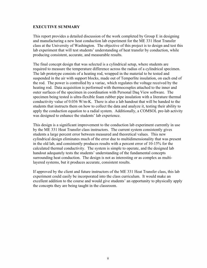
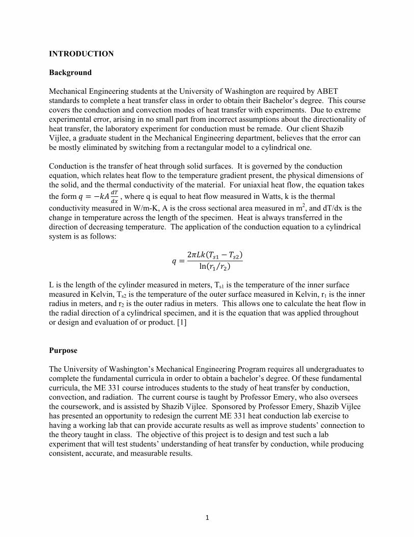
exercise must be able to complete all steps and obtain useful data in an hour or 1.5 hour session. Since the data acquisition must occur while the model is at steady state, we need to design the lab experiment to reach steady state in about one half hour. Finally, this lab must be something that can be done repeatedly and produce similar results each time. Directions for conducting the experiment and data analysis have to be simple enough for an undergraduate heat transfer class of students to follow without difficulty. CURRENT TECHNOLOGY The current setup is intended to produce conductive heat transfer through solid materials in a single direction. It consists of a plate heating element, on which rests a balsa wood block sandwiched between two aluminum plates, all of which is surrounded by layers of insulation. Thermocouples are attached to the top and bottom of the balsa wood block, and one is embedded in its geometric center. The power input to the heating element is determined by the multiplication of the voltage drawn and the current flowing through the element. The lab handout that is currently given to students in coordination with this experiment is included in Appendix A. This setup produces unreasonably high experimental error, routinely being upwards of 250% [2]. One of the critical flaws is that a large fraction of the generated heat is transferred through the insulation. The hole cut in the insulation to allow the balsa wood and aluminum to be inserted is larger than these blocks, allowing convection to occur. The aluminum and balsa wood are compressed by a heavy weight mounted on top, but there is nonetheless some contact resistance. The experiment has been run a number of times, potentially altering the physical structure of the balsa wood; the insulation shows visual evidence of heat damage. Figure 1 is a picture of this.

4

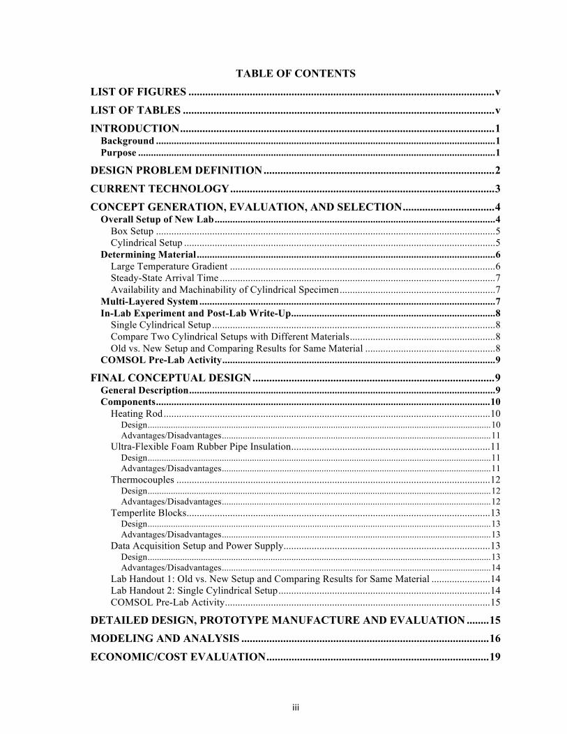
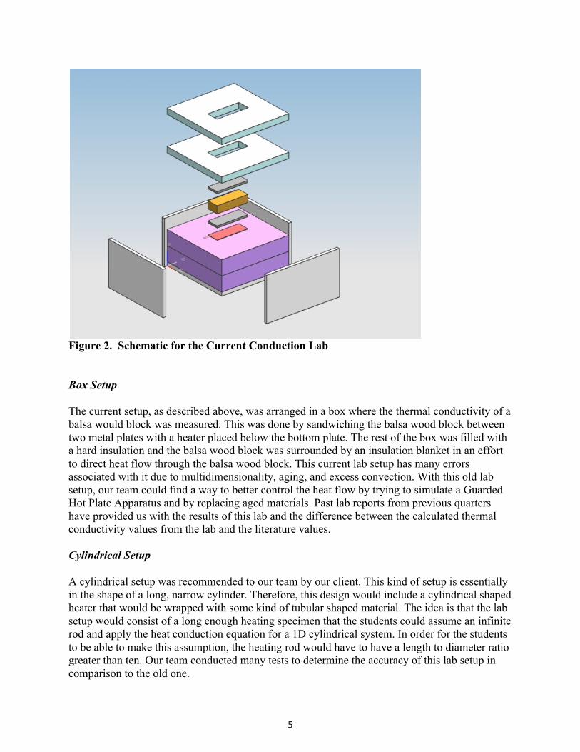
Figure 1. Current Conduction Lab Setup CONCEPT GENERATION, EVALUATION, AND SELECTION Overall Setup of New Lab The client requested that our team improve the current heat conduction lab setup. The current setup is made up of a box that measures the thermal conductivity through a balsa wood block. A schematic of this lab setup is shown in Figure 2. The client did not give us any specific requirements as to the overall setup of the lab but did suggest a cylindrical system. Therefore, our team had the option of improving the current box setup or creating and testing a new cylindrical one. Our team chose to continue working with the system that produced the most accurate results for the thermal conductivity of a material when compared to its literature value.

5

Figure 2. Schematic for the Current Conduction Lab Box Setup The current setup, as described above, was arranged in a box where the thermal conductivity of a balsa would block was measured. This was done by sandwiching the balsa wood block between two metal plates with a heater placed below the bottom plate. The rest of the box was filled with a hard insulation and the balsa wood block was surrounded by an insulation blanket in an effort to direct heat flow through the balsa wood block. This current lab setup has many errors associated with it due to multidimensionality, aging, and excess convection. With this old lab setup, our team could find a way to better control the heat flow by trying to simulate a Guarded Hot Plate Apparatus and by replacing aged materials. Past lab reports from previous quarters have provided us with the results of this lab and the difference between the calculated thermal conductivity values from the lab and the literature values. Cylindrical Setup A cylindrical setup was recommended to our team by our client. This kind of setup is essentially in the shape of a long, narrow cylinder. Therefore, this design would include a cylindrical shaped heater that would be wrapped with some kind of tubular shaped material. The idea is that the lab setup would consist of a long enough heating specimen that the students could assume an infinite rod and apply the heat conduction equation for a 1D cylindrical system. In order for the students to be able to make this assumption, the heating rod would have to have a length to diameter ratio greater than ten. Our team conducted many tests to determine the accuracy of this lab setup in comparison to the old one.

6

Determining Material When discussing what material to use for this project, our team considered three main characteristics: 1) temperature gradient across the thickness of the material, 2) steady-state arrival time, and 3) availability and/or machinablility of a cylindrical specimen. Some of the materials we talked about were metals such as aluminum, copper, and stainless steel, clay, balsa wood, pipe insulation (foam rubber and silicone foam), and Temperlite insulation. Some of these materials are compared in a Pugh Chart in Table I. Table I. Pugh Chart Comparing Characteristics of Different Materials

Characteristics

Materials

Balsa Wood (0.055

W/m∙K)

Metals

Clay (1.3

W/m∙K)

Pipe Insulation Temperlite Insulation

(0.06 W/m∙K)

Aluminum (237

W/m∙K)

Copper (401

W/m∙K)

Stainless Steels (13.4-15.1

W/m∙K)

Foam Rubber (0.036

W/m∙K)

Silicone Foam (0.056

W/m∙K)

Large Temperature Gradient

D A T U M

- - - S S S S

Quick to Steady-State + + + S S S S

Availability S S S - + + + Machinability + + + - + + - Totals Plus - 2 2 2 0 2 2 1 Minus - 1 1 1 2 0 0 1 Same - 1 1 1 2 2 2 2 Score - 1 1 1 -2 2 2 0

Large Temperature Gradient One of our functional requirements was to ensure that there was a large change in temperature, which we decided was 20°C or greater, across the thickness of the material. A temperature gradient of 20°C or more creates a more interesting lab and more importantly, allows for more accurate calculations of the thermal conductivity of the lab material. To find this we wrote a code in MATLAB using the heat conduction equation for a 1D system. The code we used is shown in Appendix B. By holding dimensions, power input, and material thickness constant and experimenting with different materials and their literature thermal conductivity values, we were able to find a relationship between thermal conductivity and the temperature gradient. We found that in order to achieve a large temperature gradient the thermal conductivity of the material should be less than about 1 W/m∙K. This means conductive materials such as metals would cause very little to no change in temperature in the lab experiment.

7

Steady-State Arrival Time Another one of our client’s requests was that our lab system reaches steady-state within a half an hour of turning it on. Steady-state means that the temperature is no longer changing with time and can be seen when the system reaches a maximum temperature and stays at this temperature for an extended period of time. We attempted to explore the mathematical theory used to calculate steady state time for various scenarios involving heat transfer, but it proved to be a more complicated analysis than we originally expected. A complete analysis and computation involves advanced differential mathematics that we felt was unnecessary given our project goals. The steady-state time was determined experimentally through our early testing. We were able to graph the change in surface temperature versus time, and see where the temperatures leveled off. Availability and Machinability of Cylindrical Specimen An issue we ran into along the way was finding cylindrical shaped materials to conduct our experiment with. Many of the materials we considered would have required special machining in order to make them the right shape. Although machining a perfect cylinder would have been difficult but doable, the bigger obstacle we ran into was being able to drill a hole the same diameter and length as the heating rod. We would have had to cut the solid cylinder into sections and drill a hole in each section individually. Then, the cylinder sections would have been stacked together which could have led to more error due to convection if the sections were not stacked tightly enough and the need to calculate contact resistances. These problems would be experienced if we worked with any of the metals or balsa wood. Balsa wood would also require special woodworking tools not readily available in the machine shop. Temperlite insulation would have been approached in the same manner but also with different tools. However, Temperlite creates a very big mess when handled, dispersing a powdery substance into the air that should not be inhaled. Clay would have been difficult to work with because we did not know how much we would need or how we would shape it. There are multiple ways to work with clay like throwing it on a pottery wheel or casting it from a mold but it would have been hard to control the exact measurements. The pipe insulations were easy to find and order off McMaster.com and even came in the dimensions we needed. The foam rubber was easier to slide onto the heating rod than the silicone foam, however. Multi-Layered System Our team discussed making a multi-layered system when we first began our concept generation, since multiple layers would demonstrate the theory surrounding contact resistances and would provide more extensive analysis in the lab write-up. To create a multi-layered system, we could have wrapped the heating rod in two layers of the same material or two different materials. However, as stated above, we had difficulty finding cylindrical materials with the right dimensions and we did not have enough time to further explore adding additional material layers.

8

In-Lab Experiment and Post-Lab Write-Up Our team had many ideas regarding how to enhance the students’ experience with this lab and to test their understanding of the heat transfer theories learned in class. In order to test the students’ knowledge about heat transfer they must complete a formal lab report with their analysis of the lab. The experiments we discussed for the students to complete were analyzing a single cylindrical system, comparing two cylindrical systems with different materials, and comparing the old lab setup vs. a new cylindrical setup when testing the same material. Single Cylindrical Setup In this lab experiment, the students would measure the temperature across the thickness, of a tubular material. By knowing the dimensions of the specimen, the thickness, the power input, and the change in temperature in the radial direction through the thickness of the material the students can calculate the thermal conductivity of the material. They can then compare the calculated thermal conductivity value with the literature one and determine the percent difference. Students would also be asked to evaluate why the calculated thermal conductivity value is different than the literature values and what aspects of the lab may contribute to the difference. This lab experiment tests the students’ understanding of heat transfer concepts but does not demand as much analysis as our team would like. Compare Two Cylindrical Setups with Different Materials This lab experiment would compare two different materials in the same cylindrical lab setup. Analysis of the lab would still require students to calculate the thermal conductivities for each of the materials and to compare them to the literature values. However, it would also ask the students to compare the thermal conductivities of the different materials and tell the students to describe why they might be so different or similar. This experiment obviously requires two cylindrical specimens to measure the thermal conductivity of. Our team was in possession of two such specimens, the foam rubber pipe insulation and the silicone foam pipe insulation, but testing of the silicone pipe insulation did not provide very similar results for thermal conductivity in comparison to the literature values. Therefore, in order to do this experiment a new material would need to be found. In addition, the foam rubber and the silicone foam pipe insulations looked alike and had similar thermal conductivities. It might be more fun for the students to analyze if the two materials that were tested were more significantly different. Old vs. New Setup and Comparing Results for Same Material The comparison of the old box setup and the new cylindrical system when testing the same material would be an interesting experiment. Like the lab experiments above, the main purpose of this lab would be to measure the thermal conductivity of the material in both the lab setups. Then the calculated thermal conductivity values would be compared to the literature values and each other. The students would then be asked to explain why the calculated thermal conductivities for each setup vary from each other and why they both may be different from the literature values. This experiment would be the most comprehensive of the three proposed experiments and formal lab write-ups but also requires that either our new cylindrical setup be

9

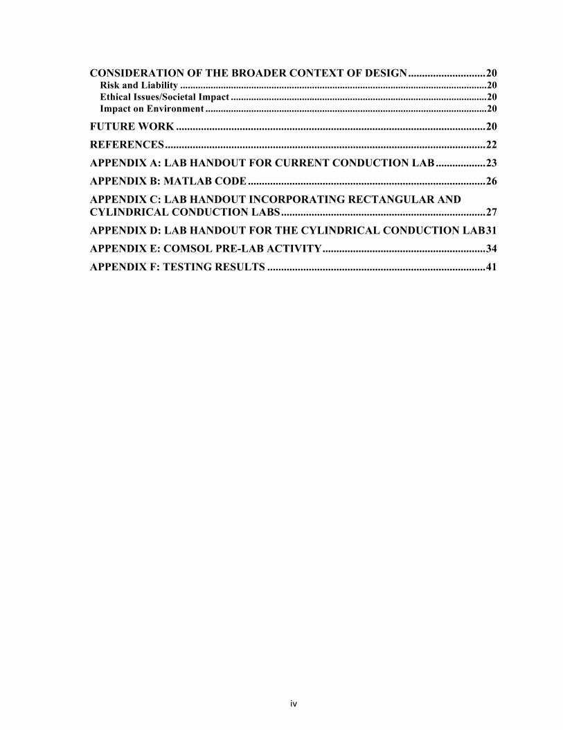
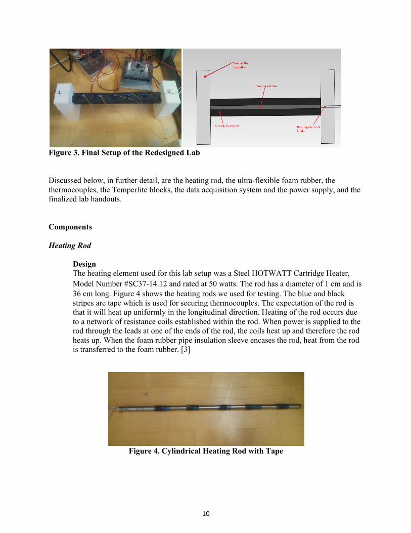
made with balsa wood or that the balsa wood in the old experiment be replaced with a new material. COMSOL Pre-Lab Activity In addition to an in-lab experience with a post-lab formal write up, our team thought a COMSOL pre-lab activity might make the experiment more engaging. COMSOL is an engineering, design, and finite element analysis software program. This was also a suggestion given to us by the client if we had time to investigate COMSOL. A COMSOL activity performed before the experiment, where students could actually see a computer simulation of how the heat is transferred through the material, would hopefully increase interest in the lab itself. Furthermore, as graduating Mechanical Engineering students from the University of Washington, we feel that we were not trained to use COMSOL very effectively and have not used it much since our first introduction to it. A step-by-step COMSOL pre-lab activity would give students the chance to become more familiar with the program. FINAL CONCEPTUAL DESIGN General Description The final design our team chose to pursue in order to achieve the clients request to improve the current heat conduction experiment utilized in ME 331: Heat Transfer was a cylindrical setup. The setup is depicted below in Figure 3, which shows a photo of the final setup as observed by the student as well as section view with labeled components. With this setup, a cylindrical heating rod is covered with an ultra-flexible foam rubber pipe insulation sleeve. Thermocouples are placed along the heating rod and the foam rubber sleeve to measure the temperature difference across the radial thickness of the foam rubber pipe insulation. The ends of the heating element and the rubber foam sleeve are supported and further insulated by two Temperlite blocks. Two small holes were made in one of the Temperlite blocks to pass the heating rod leads through, shown in the right picture of Figure 3, which carry power from the power supply to the rod itself. The power input and temperature readings from the thermocouples are gathered and displayed using the same data acquisition system, Personal Daq View, used in the old heat conduction lab. Instructions for analyzing data provided by Personal Daq View are given in the lab handout.

10

Figure 3. Final Setup of the Redesigned Lab Discussed below, in further detail, are the heating rod, the ultra-flexible foam rubber, the thermocouples, the Temperlite blocks, the data acquisition system and the power supply, and the finalized lab handouts. Components Heating Rod Design

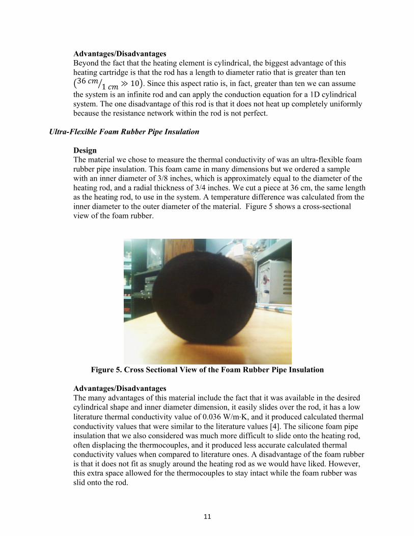
The heating element used for this lab setup was a Steel HOTWATT Cartridge Heater, Model Number #SC37-14.12 and rated at 50 watts. The rod has a diameter of 1 cm and is 36 cm long. Figure 4 shows the heating rods we used for testing. The blue and black stripes are tape which is used for securing thermocouples. The expectation of the rod is that it will heat up uniformly in the longitudinal direction. Heating of the rod occurs due to a network of resistance coils established within the rod. When power is supplied to the rod through the leads at one of the ends of the rod, the coils heat up and therefore the rod heats up. When the foam rubber pipe insulation sleeve encases the rod, heat from the rod is transferred to the foam rubber. [3]

Figure 4. Cylindrical Heating Rod with Tape

11

Advantages/Disadvantages Beyond the fact that the heating element is cylindrical, the biggest advantage of this heating cartridge is that the rod has a length to diameter ratio that is greater than ten 36 𝑐𝑚

1 𝑐𝑚 ≫ 10 . Since this aspect ratio is, in fact, greater than ten we can assume the system is an infinite rod and can apply the conduction equation for a 1D cylindrical system. The one disadvantage of this rod is that it does not heat up completely uniformly because the resistance network within the rod is not perfect.

Ultra-Flexible Foam Rubber Pipe Insulation Design

The material we chose to measure the thermal conductivity of was an ultra-flexible foam rubber pipe insulation. This foam came in many dimensions but we ordered a sample with an inner diameter of 3/8 inches, which is approximately equal to the diameter of the heating rod, and a radial thickness of 3/4 inches. We cut a piece at 36 cm, the same length as the heating rod, to use in the system. A temperature difference was calculated from the inner diameter to the outer diameter of the material. Figure 5 shows a cross-sectional view of the foam rubber.

Figure 5. Cross Sectional View of the Foam Rubber Pipe Insulation

Advantages/Disadvantages

The many advantages of this material include the fact that it was available in the desired cylindrical shape and inner diameter dimension, it easily slides over the rod, it has a low literature thermal conductivity value of 0.036 W/m∙K, and it produced calculated thermal conductivity values that were similar to the literature values [4]. The silicone foam pipe insulation that we also considered was much more difficult to slide onto the heating rod, often displacing the thermocouples, and it produced less accurate calculated thermal conductivity values when compared to literature ones. A disadvantage of the foam rubber is that it does not fit as snugly around the heating rod as we would have liked. However, this extra space allowed for the thermocouples to stay intact while the foam rubber was slid onto the rod.

12

Thermocouples Design

The thermocouples used in this lab system were Type K chromega-alomega 30 gage. They measured the temperature at desired locations along both the heating rod and the foam rubber insulation. Five thermocouples were placed approximately equidistant from each other along the length of the heating rod, as seen in Figure 6. Another five thermocouples were placed along the outside of the foam rubber insulation on the same radial lines as the thermocouples on the heating rod. The thermocouples were attached to both surfaces using flash tape, which is the blue tape visible in Figure 7. We used flash tape to fasten the thermocouples to the heated surfaces because it does not burn or affect the temperature readings of the thermocouples.

Figure 6. Placement of Thermocouples along Heating Rod

Figure 7. Placement of Thermocouples along Outside of Insulation

Advantages/Disadvantages Thermocouples provide accurate temperature readings within one or two degrees. Fortunately, with this experiment, the change in temperature is significant enough that an error of that degree will not affect the results much.

13

Temperlite Blocks Design

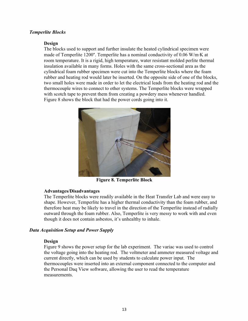
The blocks used to support and further insulate the heated cylindrical specimen were made of Temperlite 1200°. Temperlite has a nominal conductivity of 0.06 W/m∙K at room temperature. It is a rigid, high temperature, water resistant molded perlite thermal insulation available in many forms. Holes with the same cross-sectional area as the cylindrical foam rubber specimen were cut into the Temperlite blocks where the foam rubber and heating rod would later be inserted. On the opposite side of one of the blocks, two small holes were made in order to let the electrical leads from the heating rod and the thermocouple wires to connect to other systems. The Temperlite blocks were wrapped with scotch tape to prevent them from creating a powdery mess whenever handled. Figure 8 shows the block that had the power cords going into it.

Figure 8. Temperlite Block

Advantages/Disadvantages

The Temperlite blocks were readily available in the Heat Transfer Lab and were easy to shape. However, Temperlite has a higher thermal conductivity than the foam rubber, and therefore heat may be likely to travel in the direction of the Temperlite instead of radially outward through the foam rubber. Also, Temperlite is very messy to work with and even though it does not contain asbestos, it’s unhealthy to inhale.

Data Acquisition Setup and Power Supply Design

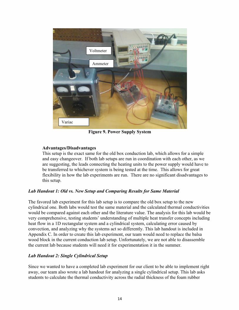
Figure 9 shows the power setup for the lab experiment. The variac was used to control the voltage going into the heating rod. The voltmeter and ammeter measured voltage and current directly, which can be used by students to calculate power input. The thermocouples were inserted into an external component connected to the computer and the Personal Daq View software, allowing the user to read the temperature measurements.

14

Figure 9. Power Supply System

Advantages/Disadvantages This setup is the exact same for the old box conduction lab, which allows for a simple and easy changeover. If both lab setups are run in coordination with each other, as we are suggesting, the leads connecting the heating units to the power supply would have to be transferred to whichever system is being tested at the time. This allows for great flexibility in how the lab experiments are run. There are no significant disadvantages to this setup.

Lab Handout 1: Old vs. New Setup and Comparing Results for Same Material The favored lab experiment for this lab setup is to compare the old box setup to the new cylindrical one. Both labs would test the same material and the calculated thermal conductivities would be compared against each other and the literature value. The analysis for this lab would be very comprehensive, testing students’ understanding of multiple heat transfer concepts including heat flow in a 1D rectangular system and a cylindrical system, calculating error caused by convection, and analyzing why the systems act so differently. This lab handout is included in Appendix C. In order to create this lab experiment, our team would need to replace the balsa wood block in the current conduction lab setup. Unfortunately, we are not able to disassemble the current lab because students will need it for experimentation it in the summer. Lab Handout 2: Single Cylindrical Setup Since we wanted to have a completed lab experiment for our client to be able to implement right away, our team also wrote a lab handout for analyzing a single cylindrical setup. This lab asks students to calculate the thermal conductivity across the radial thickness of the foam rubber

Variac

Voltmeter

Ammeter

15

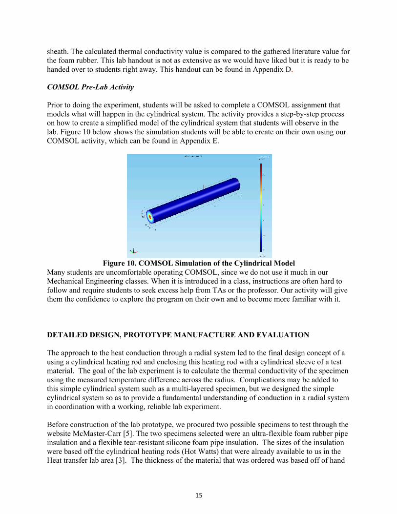
sheath. The calculated thermal conductivity value is compared to the gathered literature value for the foam rubber. This lab handout is not as extensive as we would have liked but it is ready to be handed over to students right away. This handout can be found in Appendix D. COMSOL Pre-Lab Activity Prior to doing the experiment, students will be asked to complete a COMSOL assignment that models what will happen in the cylindrical system. The activity provides a step-by-step process on how to create a simplified model of the cylindrical system that students will observe in the lab. Figure 10 below shows the simulation students will be able to create on their own using our COMSOL activity, which can be found in Appendix E.

Figure 10. COMSOL Simulation of the Cylindrical Model

Many students are uncomfortable operating COMSOL, since we do not use it much in our Mechanical Engineering classes. When it is introduced in a class, instructions are often hard to follow and require students to seek excess help from TAs or the professor. Our activity will give them the confidence to explore the program on their own and to become more familiar with it. DETAILED DESIGN, PROTOTYPE MANUFACTURE AND EVALUATION The approach to the heat conduction through a radial system led to the final design concept of a using a cylindrical heating rod and enclosing this heating rod with a cylindrical sleeve of a test material. The goal of the lab experiment is to calculate the thermal conductivity of the specimen using the measured temperature difference across the radius. Complications may be added to this simple cylindrical system such as a multi-layered specimen, but we designed the simple cylindrical system so as to provide a fundamental understanding of conduction in a radial system in coordination with a working, reliable lab experiment. Before construction of the lab prototype, we procured two possible specimens to test through the website McMaster-Carr [5]. The two specimens selected were an ultra-flexible foam rubber pipe insulation and a flexible tear-resistant silicone foam pipe insulation. The sizes of the insulation were based off the cylindrical heating rods (Hot Watts) that were already available to us in the Heat transfer lab area [3]. The thickness of the material that was ordered was based off of hand

16

calculations performed during the concept generation phase. The goal was to have a good temperature gradient of at least 20 K. This led us to order the foam rubber with a thickness of 3/4" and the silicone foam with a thickness of 7/16”. Most of the components that made up our conduction lab were sourced from the lab area to keep costs low. For example, we utilized the current and voltage generators already in the lab. Along with this, the insulating supports on the finalized design concept were constructed from blocks of Temperlite that was readily available in the lab area. Also, the thermocouples were made in-house through the guidance of Bill Kuykendall, the resident lab supervisor for the Mechanical Engineering Department. Once the materials were gathered, the prototype of the radial heat conduction lab came together rather quickly. Before building started, twenty five thermocouples were made in the heat transfer lab. Next the insulation supports were manufactured with a simple hack saw and various screwdrivers to dig fitment holes into the support blocks. Once the supports were made, the attachment of thermocouples was put onto the surface of the heating rod, outer surface of the test specimen, and in the insulation blocks. Our evaluation of the prototype began with determining the time it took for the material to reach steady state. Initial tests were longer than later trials because we needed to ensure that steady state was obtained. Typically both materials took longer than one hour to reach steady state; of which the ultra-flexible foam rubber took about 1.5 hours. Next the temperature gradient was determined and the thermal conductivity, k, was determined. Due to having thermocouple pairs along the length of the rod, we determined an overall k value by averaging the temperature difference along the rod, and also calculated specific k values relating to each thermocouple pair. To make sure consistent results could be measured, the prototype was tested various times to ensure reliability of data. The results of this testing will be discussed in analysis portion of this report. MODELING AND ANALYSIS Once the final concept was decided upon, we selected two different types of pipe insulation: ultra-flexible foam rubber pipe insulation and flexible tear-resistant silicone foam pipe insulation. Both of these had inner diameters of 3/8”, which was close to the 1 cm diameter of the heating rod. The foam rubber had a manufactured thickness of 3/4” or 1.905 cm (actual measured thickness was slightly less but calculations assume 3/8”). The silicone foam had a manufactured thickness of 7/16” or 1.11 cm (actual measured thickness was slightly greater). The foam rubber had a thermal conductivity given by the manufacture of 0.25 BTu-in/hr. ft2 °F, or 0.036 W/m-K [4]. The silicone foam had a given thermal conductivity of 0.39 BTu-in/hr. ft2 °F, or 0.056 W/m-K [5]. Testing was done on both specimens across the span of about two weeks. As explained above in previous sections, a section of each material was slipped onto the heating rod, fully encasing it. Thermocouples were placed along the inside of the insulation and along the outside so as to measure the temperature difference across the radius of the material. The same process was carried out for each test. The dimensions of the two separate materials remained constant throughout all tests. The amount of power supplied to the heating rod was

17

varied across tests to ensure that results remained consistent for different power levels. Data acquisition was carried out up through steady state. It was important to collect final temperature readings while the system was at steady state, so earlier tests were carried out over a longer duration of time so that we could obtain an accurate picture of how long it took each specimen to arrive at steady state. At the end of each test, final temperature values and the power input value were recorded and then used to calculate the thermal conductivity value via the heat conduction equation. This was done with two different methods. First, the difference between the average outside surface temperature and the average inside surface temperature was used to calculate k. The second method was to calculate a k value for each pair of outside-inside temperature readings and then average the k values. Both methods gave similar results, but it was deemed that the first method was more accurate. The test results for the foam rubber insulation were much more accurate than results obtained from the old heat transfer lab. The percent error between the measured/calculated thermal conductivity and the given manufacture value ranged between 10 and 15%. Table II shows the final measured values obtained from a test conducted on May 22, 2012. The TC values are the thermocouple measurements along the rod (1R-5R) and the outside surface (1O-5O). The calculated k value for this test was 0.041 W/m-K when using the average temperature difference to calculate k. This is a 12.94% error from the literature value. Table II. May 22, 2012 Test Results for Foam Rubber Insulation TC 1R

TC 2R

TC 3R

TC 4R

TC 5R

TC 1O

TC 2O

TC 3O

TC 40

TC 50 Power

°C °C °C °C °C °C °C °C °C °C W 87.82 85.35 80.47 76.68 70.53 31.87 32.88 32.11 32.07 31.56 2.81

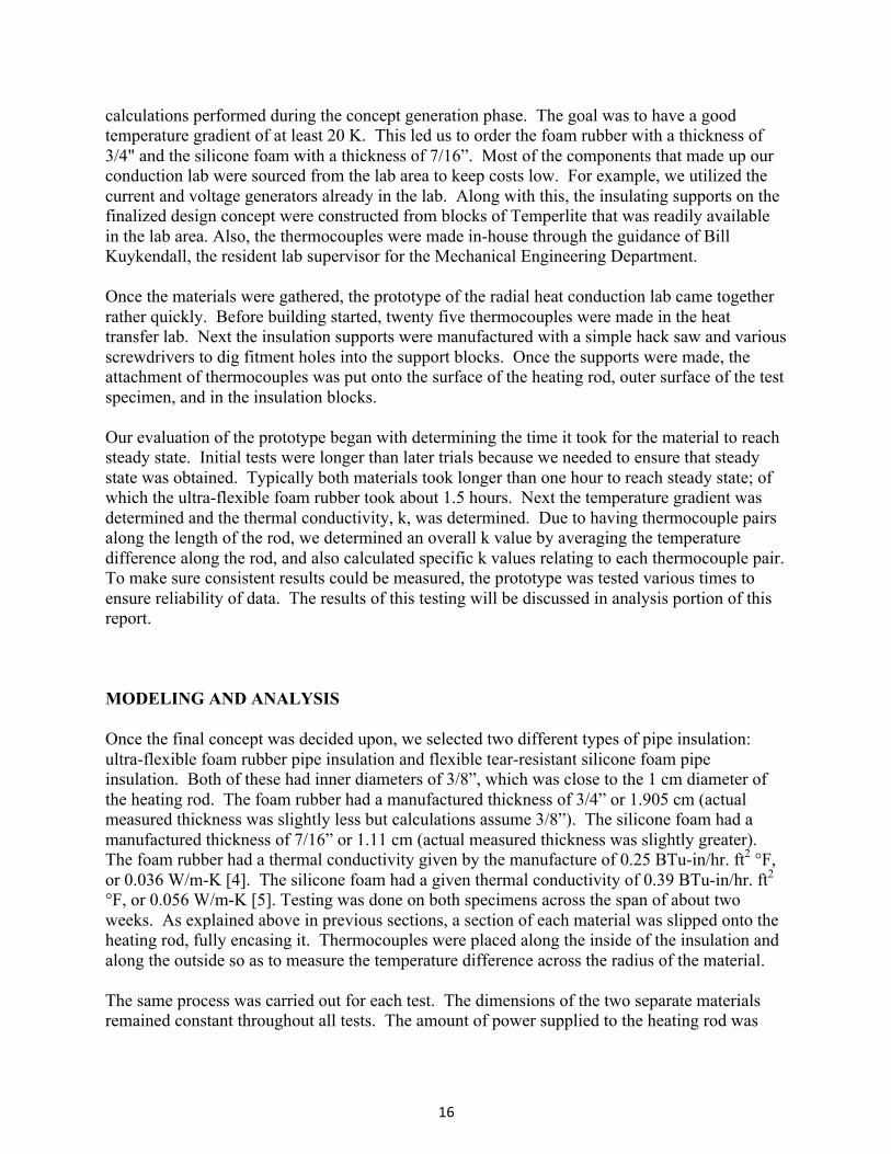
When examining how the k values changed along the length of the specimen, we noticed some reoccurring observations throughout all the tests. Temperatures at the end of the cylinder, where the power cords were attached, were noticeably lower, causing the k value calculated at the ends to have a greater difference from the literature value than the other measured k values. This led us to examine the heating elements in greater depth and conduct further research into their design. We found that the rods consisted of resistance coils spread throughout that are supposed to uniformly heat the rod. However, there is a space between the end and the start of the coils, which explained why there were lower temperature readings at the end. Figure 11 shows how the k values varied over the length of the rod for the May 22 test. The points on the right are the measurements taken from the end of the rod where the power is attached.

18

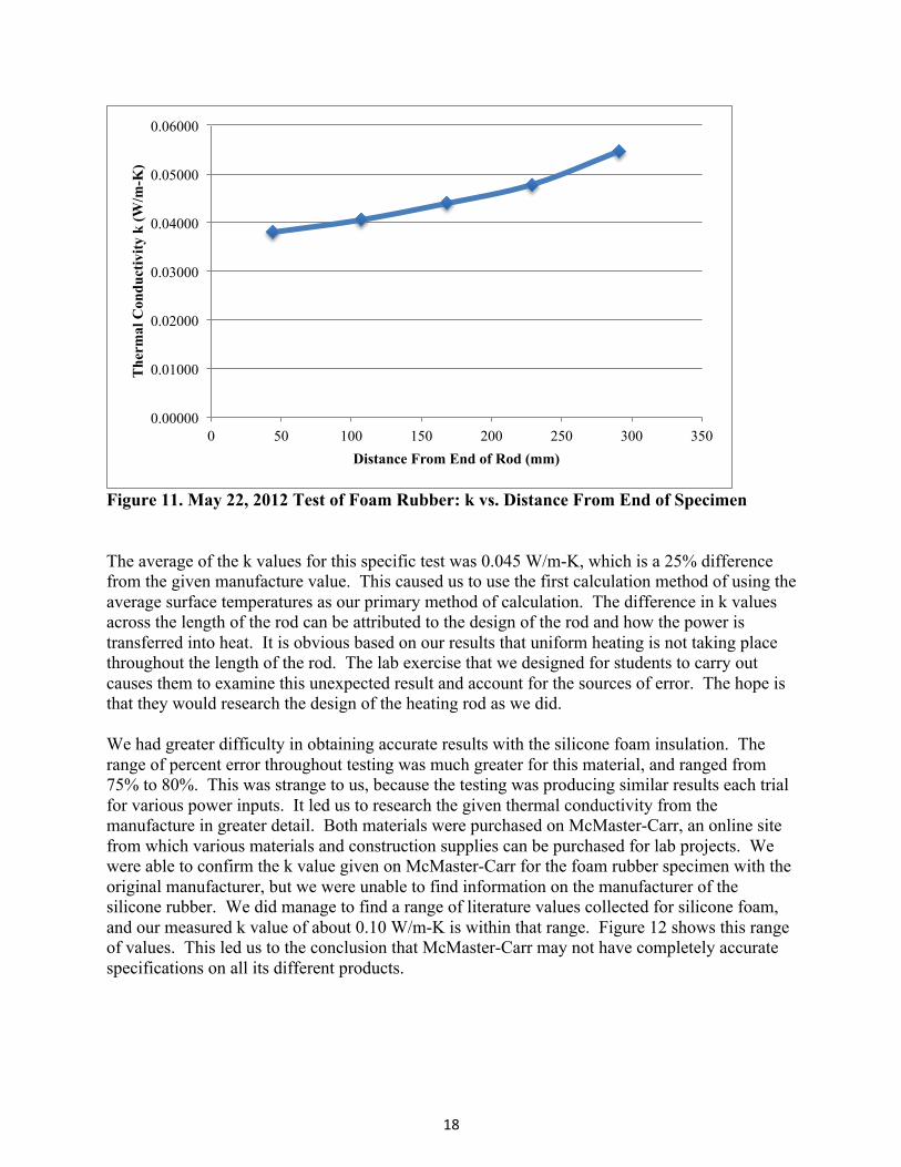
Figure 11. May 22, 2012 Test of Foam Rubber: k vs. Distance From End of Specimen The average of the k values for this specific test was 0.045 W/m-K, which is a 25% difference from the given manufacture value. This caused us to use the first calculation method of using the average surface temperatures as our primary method of calculation. The difference in k values across the length of the rod can be attributed to the design of the rod and how the power is transferred into heat. It is obvious based on our results that uniform heating is not taking place throughout the length of the rod. The lab exercise that we designed for students to carry out causes them to examine this unexpected result and account for the sources of error. The hope is that they would research the design of the heating rod as we did. We had greater difficulty in obtaining accurate results with the silicone foam insulation. The range of percent error throughout testing was much greater for this material, and ranged from 75% to 80%. This was strange to us, because the testing was producing similar results each trial for various power inputs. It led us to research the given thermal conductivity from the manufacture in greater detail. Both materials were purchased on McMaster-Carr, an online site from which various materials and construction supplies can be purchased for lab projects. We were able to confirm the k value given on McMaster-Carr for the foam rubber specimen with the original manufacturer, but we were unable to find information on the manufacturer of the silicone rubber. We did manage to find a range of literature values collected for silicone foam, and our measured k value of about 0.10 W/m-K is within that range. Figure 12 shows this range of values. This led us to the conclusion that McMaster-Carr may not have completely accurate specifications on all its different products.

0.00000

0.01000

0.02000

0.03000

0.04000

0.05000

0.06000

0 50 100 150 200 250 300 350

The

rmal

Con

duct

ivity

k (W

/m-K

)

Distance From End of Rod (mm)

19

Figure 12. Range of Thermal Conductivities for Silicone Foams [6] As a result of our testing, it was concluded that the lab exercise should be designed for the foam rubber specimen because we had a good literature value for the thermal conductivity, and testing results produced a reasonable percent error between the measured k value and the literature value. The silicone foam system was also constructed and may be used, but a more accurate literature value for the thermal conductivity should be found. All testing results can be found in Appendix F. ECONOMIC/COST EVALUATION The experiment setup requires systems for generating heat, recording data, and channeling heat. On the generation side, it requires a Variac (a controllable voltage source), a voltmeter, an ammeter, and a cartridge heater. The data recording system is composed of a data acquisition module and ten type K thermocouples, plus leads for the voltmeter and ammeter. The heat leaves the cartridge heater via the specimen material and two side blocks of Temperlite. Most of these materials were readily available in the heat transfer lab space. The specimen material had to be purchased. Two specimens were acquired, one made of foam rubber ($5.13 for a 6-foot specimen, plus $16.80 for a quarter-inch thick sheet needed for the old setup to be

20

rebuilt), and the other of silicone foam ($54.80 for six feet, which was much higher than expected) [5]. With shipping costs included, the entire cost to the group was $94.82, much lower than the client’s initial budget estimate of $1,000. CONSIDERATION OF THE BROADER CONTEXT OF DESIGN Risk and Liability There are two ways the setup could pose danger to people around it. The first is through thermal damage—either burning people directly, or starting fires. Fire danger is mitigated by keeping the cartridge heater’s outer temperature below the maximum operating temperature of the material specimen. For the foam rubber, this was about one hundred degrees Celsius, and this temperature was only slightly increased for the silicone foam. A person cannot directly experience this temperature due to the layer of insulation. We found that the outer temperature was between 30 and 50 degrees Celsius, not enough to cause harm to a person. The second mode of peril is through electrical shock. However, the power delivered to the cartridge heater is around 4 watts, removing any real danger of electrocution. Ethical Issues/Societal Impact The original motivation of modifying the current conduction experiment was that the experimental error was out of control. Such an inaccurate experiment does not engender a sense of trust and professional responsibility in the students who perform it. It is perhaps not entirely ethical to claim to have taught something to someone when the method of teaching does not actually demonstrate what should have been taught. Therefore, with the considerably lower percent error we achieved, we have acted ethically. Impact on Environment The amount of waste involved in creating the experiment setup was relatively low. Leftover insulation will remain in the heat transfer lab and hopefully be usable in another project. The amount of energy consumed by the experiment setup is negligible, and regardless is supplied primarily by clean hydropower thanks to Washington’s extensive dam system. FUTURE WORK The lab experiment that we designed is fully ready to be incorporated into the ME 331 Heat Transfer class curriculum, but there are many things that could be done to improve or modify the lab experience.

21

It is highly recommended that the cylindrical system and the corresponding lab exercise that we designed be made part of the existing heat conduction lab. We have included a lab handout in Appendix C that achieves this goal. The plan is that students would be able to compare the accuracy of the box system to that of the cylindrical system. The large sources of error in the box system would become more evident, and the students would be able to conduct a more fruitful analysis. In order to make this modification, the balsa wood that is the current specimen in the box system must be replaced with flat sheets of the foam rubber insulation to be consistent with the cylindrical system. We have purchased sheets of this material and cut it into suitable sections ready to be inserted into the box system. We were advised by our client not to dismantle the current setup in case it is used as it is for summer classes, so we were not able to finalize this step. It would take a few days to dismantle the current setup, replace the balsa wood with the rubber foam, insert thermocouples throughout the system, and replace the insulation surrounding the specimen. This should be done upon approval by the ME 331 instructor. Additionally, we have several recommendations for future work in regards to improving the cylindrical system and making the lab exercise more interesting to students. The system is setup so that cylinders of different materials can be swapped in and out. Research should be done into procuring a cylindrical specimen made out of balsa wood, to match the current box system specimen, as well as a ceramic specimen. Thermal conductivity values for ceramics are generally higher than those for the pipe insulation that we used, but are still low enough to produce a measurable temperature difference in the specimen. Because of the higher conductivity value, the specimen would reach steady state faster, which would potentially allow the students to conduct the entire experiment themselves. With the pipe insulation, it takes about 1.5 hours for the system to reach steady state, which is too long for students to sit in the lab waiting for results. Using a ceramic would hopefully shorten that waiting time, allowing the students to turn on the system themselves and observe the entire conduction process from start to finish. Another complication that should be considered is the inclusion of multiple layers. Using multiple layers of the same material, or even different materials, would allow students to plot the changes in temperature across the total radius of the system. It would also introduce the concept of contact resistance, which would result in a more intricate analysis for the students. It is also recommended that further research be conducted into the theoretical calculation of the time it takes for a cylindrical conduction system to reach steady state. This goes beyond what is required for the undergraduate curriculum as it involves a higher level of understanding of difficult mathematical concepts, but it would be helpful to be able to accurately predict the steady state time for the system.

22

REFERENCES [1] F. P. Incropera et al., Introduction to Heat Transfer, 5th ed. Hoboken, NJ: Wiley, 2007. [2] M. R. Buckley et al., “Conduction Heat Transfer Lab,” Heat Transfer Class, Univ. Washington, Seattle, WA, June 2011. [3] Hotwatt: Heaters For Every Application [Online]. Available: http://www.hotwatt.com [4] “ ‘R’ Value for AP Armaflex,” Armacell Engineered Foams, Mebane, NC, Nov. 2010. [5] McMaster-Carr [Online]. Available: http://www.mcmaster.com/# [6] H. Zhang and A. Cloud, “New Advances in Silicone-based Thermal Insulation,” Arlon Silicone Technologies, Bear, DE.

23

APPENDIX A: LAB HANDOUT FOR CURRENT CONDUCTION LAB CONDUCTION HEAT TRANSFER EXPERIMENT The purpose of this experiment is to determine the thermal conductivity of low k materials through direct measurement. INTRODUCTION AND BACKGROUND The basis for analysis of conduction heat transfer situations is known as Fourier's Law Of Heat Conduction. The “Law” which is so glibly pronounced as an obvious truth was submitted as part of a 234 page paper by Joseph Fourier in 1807. The work was controversial, and it remained unpublished until 1822. Compare this publication rate with that of any assistant professor today! No tenure for Joseph. The empirical law that he stated is “The heat flux resulting from thermal conduction is proportional to the magnitude of the temperature gradient and opposite to it in sign”. Note that he did not state that heat flux is directly proportional to the first power of the gradient: it is just proportional. This experiment is designed to measure the value of the proportionality factor through knowledge of the heat flux, temperature difference, and the distance of conduction. APPARATUS The apparatus if very straightforward and simple. An electric heater, which is potted in silicone, is used to heat the bottom aluminum plate whose inner surface has thermocouples set in to it. The paper stack is covered by the top aluminum plate having thermocouples on its inner surface. A thermocouple is also located in the geometric center of the stack. The stack is insulated on the bottom with Temperlite 2000 insulation and on the four sides with an insulation blanket. The applied heating current and electric potential are measured with meters, and the power generated by the heater can be determined by the relation P = IV, where I is current, and V is potential. A single thermocouple is mounted in the vicinity of a glass thermometer to measure ambient temperature. The overall thickness of the paper stack is 1.00 inches and it is sandwiched between the two 0.25 inch thick aluminum plates for a total stack thickness of 1.50 inches (one inch is 0.0254 m). MEASUREMENTS Measurements are taken with a data acquisition system which measures 10 temperatures and the power to the heater is calculated by using the potential from the power source and the current from the multimeter. When taking measurements, be sure and note on paper the time of the experiment and the following: 1) the ambient temperature as indicated by the meter on the shelf above the experiment; 2) the electric potential across the heater as indicated by the leftmost voltmeter above the experiment; 3) the current through the heater as indicated by the rightmost voltmeter. These values will be used to check the heater power measured by the DAQ and the ambient temperature. Three temperatures on the bottom plate (tc 1, 2, 3), in the middle of the paper (tc 4), on the top plate (tc 5, 6, 7), and the ambient temperature (tc 8). Average the temperatures over time and on each plate and express the result as some nominal value centered within uncertainty (±) limits. You can judge the uncertainty of the measurements by watching the fluctuations of the readings. Record at least 10 sets of measurements in order to get some statistical idea of the fluctuations.

24

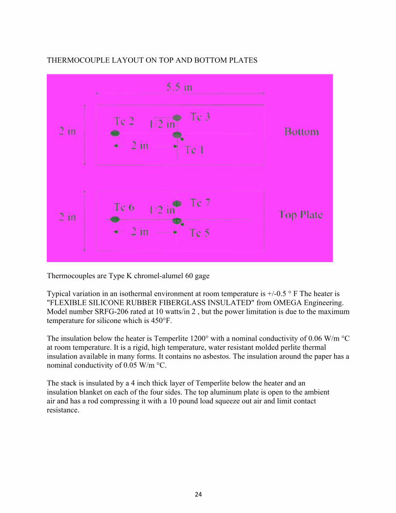
THERMOCOUPLE LAYOUT ON TOP AND BOTTOM PLATES

Thermocouples are Type K chromel-alumel 60 gage Typical variation in an isothermal environment at room temperature is +/-0.5 ° F The heater is "FLEXIBLE SILICONE RUBBER FIBERGLASS INSULATED" from OMEGA Engineering. Model number SRFG-206 rated at 10 watts/in 2 , but the power limitation is due to the maximum temperature for silicone which is 450°F. The insulation below the heater is Temperlite 1200° with a nominal conductivity of 0.06 W/m °C at room temperature. It is a rigid, high temperature, water resistant molded perlite thermal insulation available in many forms. It contains no asbestos. The insulation around the paper has a nominal conductivity of 0.05 W/m °C. The stack is insulated by a 4 inch thick layer of Temperlite below the heater and an insulation blanket on each of the four sides. The top aluminum plate is open to the ambient air and has a rod compressing it with a 10 pound load squeeze out air and limit contact resistance.

25

ANALYSIS AND DISCUSSION 1. Assuming that the mid-stack thermocouple is exactly centered between the aluminum plates, if the mid-stack temperature is not exactly at the mid-point temperature calculated from the aluminum plate temperatures explain why. Describe an experiment(s) that could be conducted to justify your reasoning. 2. Calculate the thermal conductivity of the paper sample. State what assumptions you have made in computing the heat loss. 3. Compare the measured values of thermal conductivity for the paper sample with values published in the open literature (at least three cited sources. Sources can be found in the engineering library). Do the values seem reasonable? 4. If the measured thermal conductivity values are higher than the average of the published values, then perhaps heat loss effects in the experiment were underestimated. Accounting for heat loss effects beneath the heating pad, by how much would the measured values of thermal conductivity change? 5. If the measured thermal conductivity values are less than the average of the published values, then perhaps contact resistance between adjacent paper layers influenced the results. If the results exhibit this behavior, assume that the actual thermal conductivity of the paper sample (composed of 200 layers) is the average of the three published values and calculate the contact resistance between adjacent paper layers in m2-K/W based on the actual heat transfer rate through the paper stack. Are the results seen reasonable when compared to typical contact resistance values tabulated in Table 3.2 from the textbook? 6. The experiment was conducted with insulation (ki = 0.05 W/m K) surrounding the aluminum plate/paper stack, except for the outer surface of the top plate which was exposed to atmospheric air (ka = 0.03 W/m K). Even though as air is a better insulator than the blanket insulation used (air has a lower thermal conductivity), why weren’t the four side walls of the stack exposed to atmospheric air during the experiment to lower the heat loss through these walls? Justify your answer with back-up calculations.

26

APPENDIX B: MATLAB CODE %Conduction experiment simulation clc clear all; %All units in meters, watts, Celsius %Total length, l L = 0.15; %cartridge heater generation capability, qgen qgen = 20; %estimated convection coefficient h= 100; %Ambient temperature tamb = 25 %Conduction resistant calculation %copy and alter variables as needed for multi-layer %Outer section outer radius osor = 12.7E-3; %outer section inner radius osir= 6.355E-3; %outer section conductivity (k) osk = 13.4; %outer section thermal resistance ro = (log(osor/osir))/(2*pi*osk*L); %convection resistance rh = 1/(h*2*pi*osor*L); %total resistance rtot = ro + rh; %Highest allowable temperature for surface of cartridge heater tch = qgen*rtot + tamb %outer surface area (for reference) A = osor*2*pi*L %Surface temperature of outer layer ts = qgen/(h*A) + tamb

27

APPENDIX C: LAB HANDOUT INCORPORATING RECTANGULAR AND CYLINDRICAL CONDUCTION LABS

CONDUCTION HEAT TRANSFER EXPERIMENT The purpose of this experiment is to determine the thermal conductivity of low k materials through direct measurement. INTRODUCTION AND BACKGROUND The basis for analysis of conduction heat transfer situations is known as Fourier's Law of Heat Conduction. The “Law” was submitted as part of a 234 page paper by Joseph Fourier in 1807, but was not published until 1822. The empirical law that he stated is: “The heat flux resulting from thermal conduction is proportional to the magnitude of the temperature gradient and opposite to it in sign”. Note that he did not state that heat flux is directly proportional to the first power of the gradient: it is just proportional. This experiment is designed to measure the value of the proportionality factor through knowledge of the heat flux, temperature difference, and the distance of conduction. APPARATUS Two apparatuses will be used and compared in this experiment.

1. The first apparatus consists of an electric heater, potted in silicone, which is used to heat the bottom aluminum plate whose top surface has thermocouples set into it. The rubber foam insulation sheet is sandwiched between the two aluminum plates with the top aluminum plate having thermocouples set into its bottom surface. A thermocouple is also located in the geometric center of the sheet of insulation. The sheet is insulated on the bottom with Temperlite 1200° insulation and on the four sides with an insulation blanket. The overall thickness of the rubber foam insulation sheet is 1.00 inches that is sandwiched between the two 0.25 inch thick aluminum plates for a total thickness of 1.50 inches (one inch is 0.0254 m).

2. The second apparatus has a cylindrical set-up. The electric heater used is in the shape of a

cylinder rod with a diameter of 0.393 inches (1 cm) and a length of 14.173 inches (36 cm). Thermocouples are attached along the heating element in the axial direction. The heater is covered by a tubular-shaped rubber foam pipe insulation that slides directly onto the heating rod. The rubber foam insulation has an inner diameter approximately equal to the diameter of the heating element and a thickness of 0.75 inches. Another set of thermocouples are attached to the outer surface of the rubber foam insulation. The ends of the heating rod and cylindrical rubber foam insulation are supported and insulated by blocks of Temperlite 1200°.

28

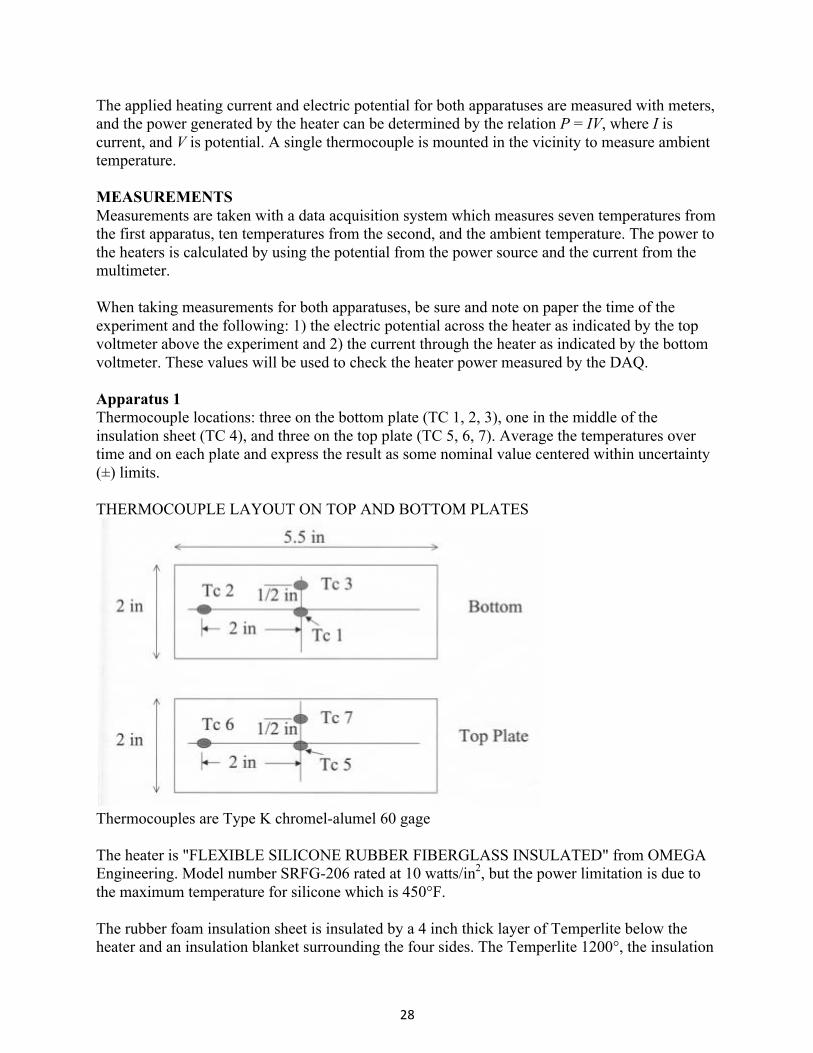
The applied heating current and electric potential for both apparatuses are measured with meters, and the power generated by the heater can be determined by the relation P = IV, where I is current, and V is potential. A single thermocouple is mounted in the vicinity to measure ambient temperature. MEASUREMENTS Measurements are taken with a data acquisition system which measures seven temperatures from the first apparatus, ten temperatures from the second, and the ambient temperature. The power to the heaters is calculated by using the potential from the power source and the current from the multimeter. When taking measurements for both apparatuses, be sure and note on paper the time of the experiment and the following: 1) the electric potential across the heater as indicated by the top voltmeter above the experiment and 2) the current through the heater as indicated by the bottom voltmeter. These values will be used to check the heater power measured by the DAQ. Apparatus 1 Thermocouple locations: three on the bottom plate (TC 1, 2, 3), one in the middle of the insulation sheet (TC 4), and three on the top plate (TC 5, 6, 7). Average the temperatures over time and on each plate and express the result as some nominal value centered within uncertainty (±) limits. THERMOCOUPLE LAYOUT ON TOP AND BOTTOM PLATES

Thermocouples are Type K chromel-alumel 60 gage The heater is "FLEXIBLE SILICONE RUBBER FIBERGLASS INSULATED" from OMEGA Engineering. Model number SRFG-206 rated at 10 watts/in2, but the power limitation is due to the maximum temperature for silicone which is 450°F. The rubber foam insulation sheet is insulated by a 4 inch thick layer of Temperlite below the heater and an insulation blanket surrounding the four sides. The Temperlite 1200°, the insulation

29

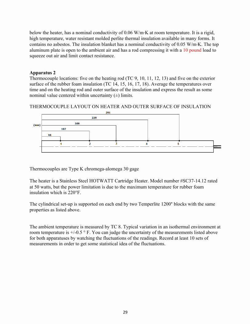
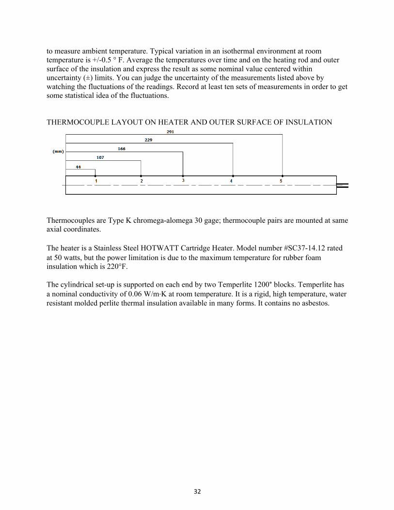
below the heater, has a nominal conductivity of 0.06 W/m∙K at room temperature. It is a rigid, high temperature, water resistant molded perlite thermal insulation available in many forms. It contains no asbestos. The insulation blanket has a nominal conductivity of 0.05 W/m∙K. The top aluminum plate is open to the ambient air and has a rod compressing it with a 10 pound load to squeeze out air and limit contact resistance. Apparatus 2 Thermocouple locations: five on the heating rod (TC 9, 10, 11, 12, 13) and five on the exterior surface of the rubber foam insulation (TC 14, 15, 16, 17, 18). Average the temperatures over time and on the heating rod and outer surface of the insulation and express the result as some nominal value centered within uncertainty (±) limits. THERMOCOUPLE LAYOUT ON HEATER AND OUTER SURFACE OF INSULATION

Thermocouples are Type K chromega-alomega 30 gage The heater is a Stainless Steel HOTWATT Cartridge Heater. Model number #SC37-14.12 rated at 50 watts, but the power limitation is due to the maximum temperature for rubber foam insulation which is 220°F. The cylindrical set-up is supported on each end by two Temperlite 1200° blocks with the same properties as listed above. The ambient temperature is measured by TC 8. Typical variation in an isothermal environment at room temperature is +/-0.5 ° F. You can judge the uncertainty of the measurements listed above for both apparatuses by watching the fluctuations of the readings. Record at least 10 sets of measurements in order to get some statistical idea of the fluctuations.

30

ANALYSIS AND DISCUSSION Part A: Apparatus 1

1. Calculate the thermal conductivity of the rubber foam sample. State what assumptions you have made in computing the heat loss.

2. Compare the measured values of thermal conductivity for the rubber foam sample with values published in the open literature. Note: the rubber foam insulation is manufactured by Armaflex. Do the values seem reasonable?

3. Account for any differences between the measured values of thermal conductivity and the literature values? What potential sources of error are there? Estimate the heat loss due to each potential source.

4. The experiment was conducted with insulation (ki = 0.05 W/m K) surrounding the

aluminum plate/rubber foam stack, except for the outer surface of the top plate which was exposed to atmospheric air (ka = 0.03 W/m K). Even though as air is a better insulator than the blanket insulation used (air has a lower thermal conductivity), why weren’t the four side walls of the stack exposed to atmospheric air during the experiment to lower the heat loss through these walls? Justify your answer with back-up calculations.

Part B: Apparatus 2

1. Calculate the thermal conductivity of the rubber foam sample using two methods: a. Take an average of the outside surface temperatures and an average of the inside

surface temperatures. Use the difference between these two to calculate a total k value.

b. Calculate separate k values for each pair of thermocouples. Average these k values.

2. Compare the measured values of thermal conductivity for the rubber foam sample with values published in the open literature. Do the values seem reasonable?


4. Construct a graph of temperature vs. longitudinal distance for the outside surface thermocouples and the inside surface thermocouples. Set x=0 for the end of the cylinder that is attached to the power supply. Does temperature vary in the longitudinal direction? Comment on why this may be.

Part C: Compare and Contrast the Two Systems Are the measured k values different for the two apparatuses? Does one system produce more accurate results than the other? Which one? Why do you think this is? Analyze the differences and similarities between the two systems. What stays constant in both setups? What changes? How does this affect your calculations?

31

APPENDIX D: LAB HANDOUT FOR THE CYLINDRICAL CONDUCTION LAB

CONDUCTION HEAT TRANSFER EXPERIMENT The purpose of this experiment is to determine the thermal conductivity of low k materials through direct measurement. INTRODUCTION AND BACKGROUND The basis for analysis of conduction heat transfer situations is known as Fourier's Law of Heat Conduction. The “Law” was submitted as part of a 234 page paper by Joseph Fourier in 1807, but was not published until 1822. The empirical law that he stated is: “The heat flux resulting from thermal conduction is proportional to the magnitude of the temperature gradient and opposite to it in sign”. Note that he did not state that heat flux is directly proportional to the first power of the gradient: it is just proportional. This experiment is designed to measure the value of the proportionality factor through knowledge of the heat flux, temperature difference, and the distance of conduction. APPARATUS The apparatus has a cylindrical set-up. The electric heater used is in the shape of a cylinder rod with a diameter of 0.393 inches (1 cm) and a length of 14.173 inches (36 cm). Thermocouples are attached along the heating element in the axial direction. The heater is covered by a tubular-shaped rubber foam pipe insulation that slides directly onto the heating rod. The rubber foam insulation has an inner diameter approximately equal to the diameter of the heating element and a thickness of 0.75 inches. Another set of thermocouples are attached to the outer surface of the rubber foam insulation. The ends of the heating rod and cylindrical rubber foam insulation are supported and insulated by blocks of Temperlite 1200°. The applied heating current and electric potential for the both apparatus are measured with meters, and the power generated by the heater can be determined by the relation P = IV, where I is current, and V is potential. A single thermocouple is mounted in the vicinity to measure ambient temperature. MEASUREMENTS Measurements are taken with a data acquisition system which measures eleven temperatures and the power to the heaters is calculated by using the potential from the power source and the current from the multimeter. When taking measurements, be sure and note on paper the time of the experiment and the following: 1) the electric potential across the heater as indicated by the top voltmeter above the experiment and 2) the current through the heater as indicated by the bottom voltmeter. These values will be used to check the heater power measured by the DAQ. Thermocouple locations: five on the heating rod (TC 1, 2, 3, 4, 5), five on the exterior surface of the rubber foam insulation (TC 6, 7, 8, 9, 10), and one in the vicinity of the experimental set-up

32

to measure ambient temperature. Typical variation in an isothermal environment at room temperature is +/-0.5 ° F. Average the temperatures over time and on the heating rod and outer surface of the insulation and express the result as some nominal value centered within uncertainty (±) limits. You can judge the uncertainty of the measurements listed above by watching the fluctuations of the readings. Record at least ten sets of measurements in order to get some statistical idea of the fluctuations. THERMOCOUPLE LAYOUT ON HEATER AND OUTER SURFACE OF INSULATION

Thermocouples are Type K chromega-alomega 30 gage; thermocouple pairs are mounted at same axial coordinates. The heater is a Stainless Steel HOTWATT Cartridge Heater. Model number #SC37-14.12 rated at 50 watts, but the power limitation is due to the maximum temperature for rubber foam insulation which is 220°F. The cylindrical set-up is supported on each end by two Temperlite 1200° blocks. Temperlite has a nominal conductivity of 0.06 W/m∙K at room temperature. It is a rigid, high temperature, water resistant molded perlite thermal insulation available in many forms. It contains no asbestos.

33

ANALYSIS AND DISCUSSION 1. Calculate the thermal conductivity of the rubber foam sample using two methods:

c. Take an average of the outside surface temperatures and an average of the inside surface temperatures. Use the difference between these two to calculate a total k value.

d. Calculate separate k values for each pair of thermocouples. Average these k values.

2. Compare the measured values of thermal conductivity for the rubber foam sample with values published in the open literature. Note: the rubber foam insulation is manufactured by Armaflex. Do the values seem reasonable?


4. Construct a graph of temperature vs. longitudinal distance for the outside surface thermocouples and the inside surface thermocouples. Set x=0 for the end of the cylinder that is attached to the power supply. Does temperature vary in the longitudinal direction? Comment on why this may be. Hint: how are the heating rods designed?

5. In general, how are thermal conductivities measured to obtain the literature values? How

does this apparatus compare to other methods?

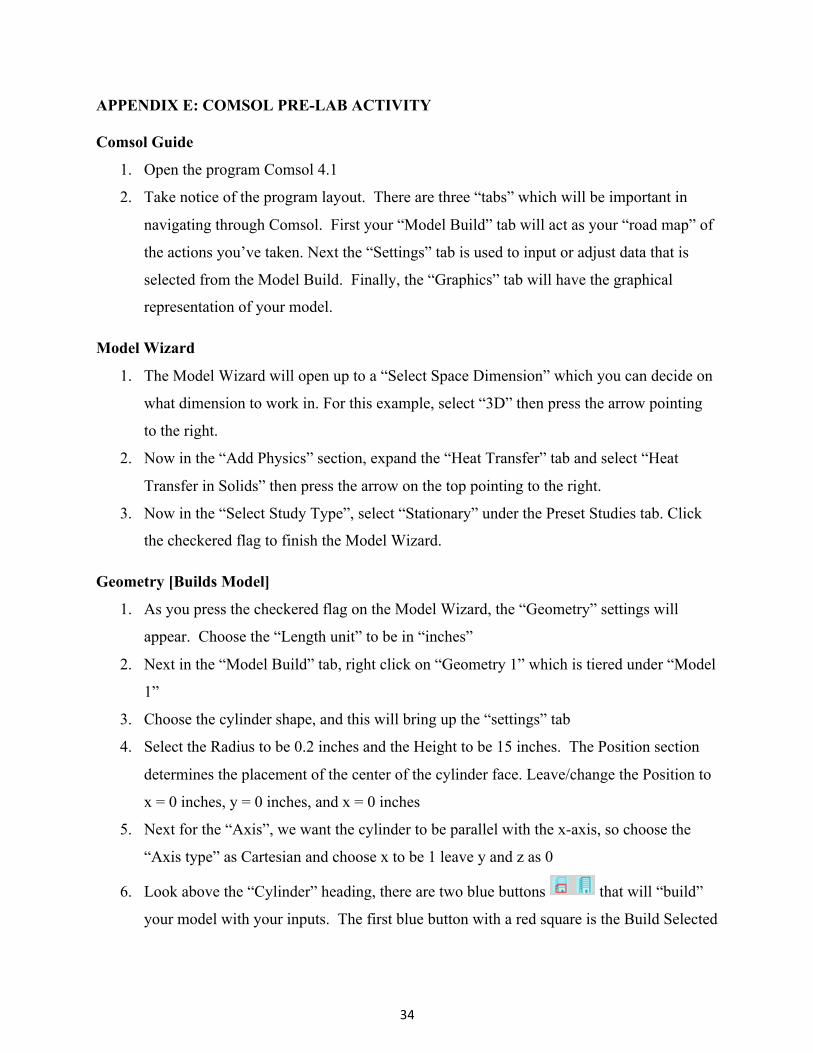
34

APPENDIX E: COMSOL PRE-LAB ACTIVITY Comsol Guide

1. Open the program Comsol 4.1

2. Take notice of the program layout. There are three “tabs” which will be important in

navigating through Comsol. First your “Model Build” tab will act as your “road map” of

the actions you’ve taken. Next the “Settings” tab is used to input or adjust data that is

selected from the Model Build. Finally, the “Graphics” tab will have the graphical

representation of your model.

Model Wizard

1. The Model Wizard will open up to a “Select Space Dimension” which you can decide on

what dimension to work in. For this example, select “3D” then press the arrow pointing

to the right.

2. Now in the “Add Physics” section, expand the “Heat Transfer” tab and select “Heat

Transfer in Solids” then press the arrow on the top pointing to the right.

3. Now in the “Select Study Type”, select “Stationary” under the Preset Studies tab. Click

the checkered flag to finish the Model Wizard.

Geometry [Builds Model]

1. As you press the checkered flag on the Model Wizard, the “Geometry” settings will

appear. Choose the “Length unit” to be in “inches”

2. Next in the “Model Build” tab, right click on “Geometry 1” which is tiered under “Model

1”

3. Choose the cylinder shape, and this will bring up the “settings” tab

4. Select the Radius to be 0.2 inches and the Height to be 15 inches. The Position section

determines the placement of the center of the cylinder face. Leave/change the Position to

x = 0 inches, y = 0 inches, and x = 0 inches

5. Next for the “Axis”, we want the cylinder to be parallel with the x-axis, so choose the

“Axis type” as Cartesian and choose x to be 1 leave y and z as 0

6. Look above the “Cylinder” heading, there are two blue buttons that will “build”

your model with your inputs. The first blue button with a red square is the Build Selected

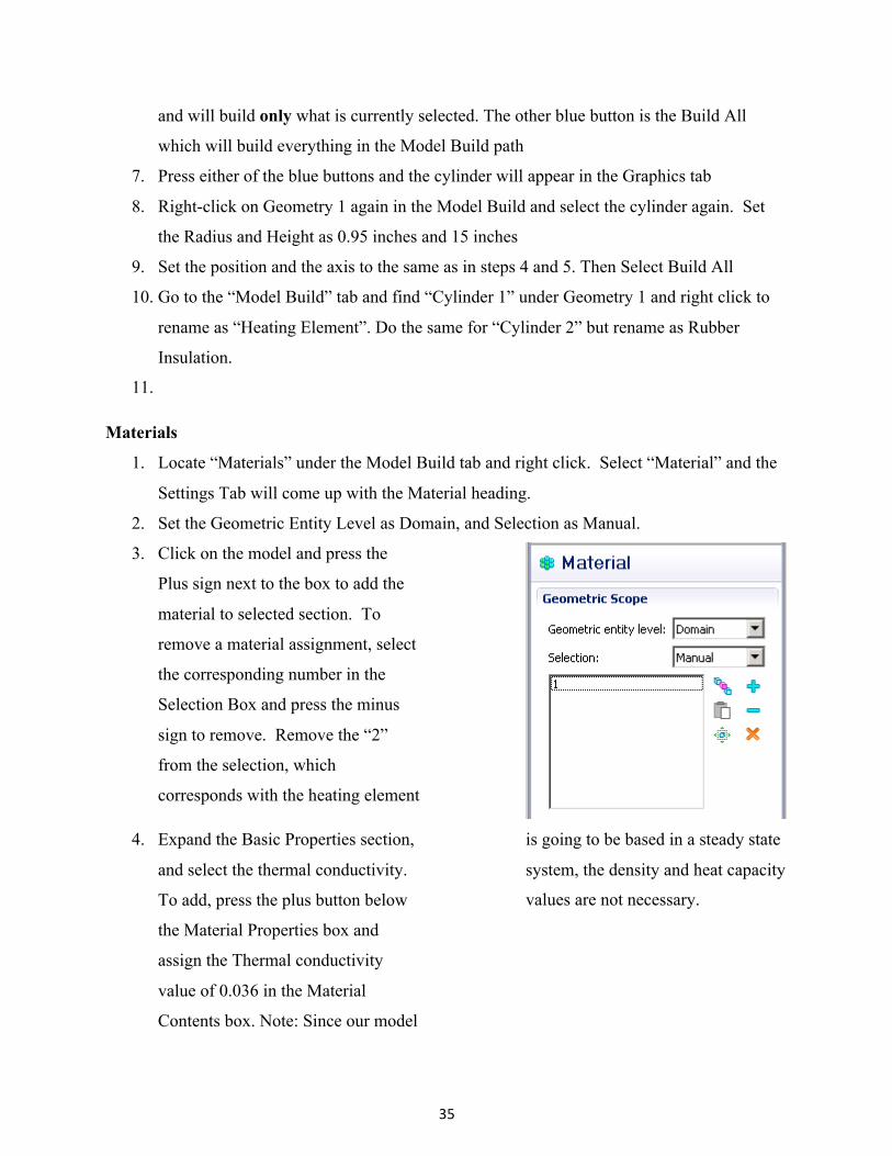
35

and will build only what is currently selected. The other blue button is the Build All

which will build everything in the Model Build path

7. Press either of the blue buttons and the cylinder will appear in the Graphics tab

8. Right-click on Geometry 1 again in the Model Build and select the cylinder again. Set

the Radius and Height as 0.95 inches and 15 inches

9. Set the position and the axis to the same as in steps 4 and 5. Then Select Build All

10. Go to the “Model Build” tab and find “Cylinder 1” under Geometry 1 and right click to

rename as “Heating Element”. Do the same for “Cylinder 2” but rename as Rubber

Insulation.

11.

Materials

1. Locate “Materials” under the Model Build tab and right click. Select “Material” and the

Settings Tab will come up with the Material heading.

2. Set the Geometric Entity Level as Domain, and Selection as Manual.

3. Click on the model and press the

Plus sign next to the box to add the

material to selected section. To

remove a material assignment, select

the corresponding number in the

Selection Box and press the minus

sign to remove. Remove the “2”

from the selection, which

corresponds with the heating element

4. Expand the Basic Properties section,

and select the thermal conductivity.

To add, press the plus button below

the Material Properties box and

assign the Thermal conductivity

value of 0.036 in the Material

Contents box. Note: Since our model

is going to be based in a steady state

system, the density and heat capacity

values are not necessary.

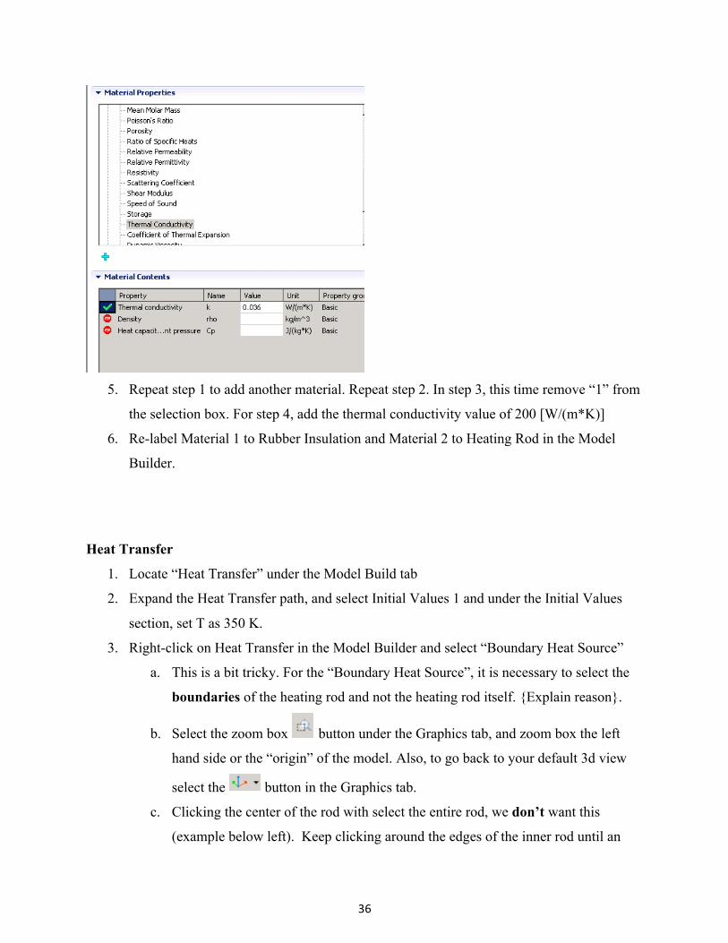
36

5. Repeat step 1 to add another material. Repeat step 2. In step 3, this time remove “1” from

the selection box. For step 4, add the thermal conductivity value of 200 [W/(m*K)]

6. Re-label Material 1 to Rubber Insulation and Material 2 to Heating Rod in the Model

Builder.

Heat Transfer

1. Locate “Heat Transfer” under the Model Build tab

2. Expand the Heat Transfer path, and select Initial Values 1 and under the Initial Values

section, set T as 350 K.

3. Right-click on Heat Transfer in the Model Builder and select “Boundary Heat Source”

a. This is a bit tricky. For the “Boundary Heat Source”, it is necessary to select the

boundaries of the heating rod and not the heating rod itself. {Explain reason}.

b. Select the zoom box button under the Graphics tab, and zoom box the left

hand side or the “origin” of the model. Also, to go back to your default 3d view

select the button in the Graphics tab.

c. Clicking the center of the rod with select the entire rod, we don’t want this

(example below left). Keep clicking around the edges of the inner rod until an

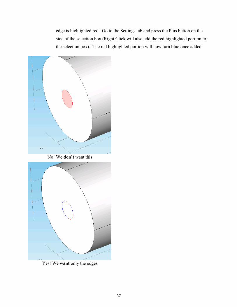
37

edge is highlighted red. Go to the Settings tab and press the Plus button on the

side of the selection box (Right Click will also add the red highlighted portion to

the selection box). The red highlighted portion will now turn blue once added.

No! We don’t want this

Yes! We want only the edges

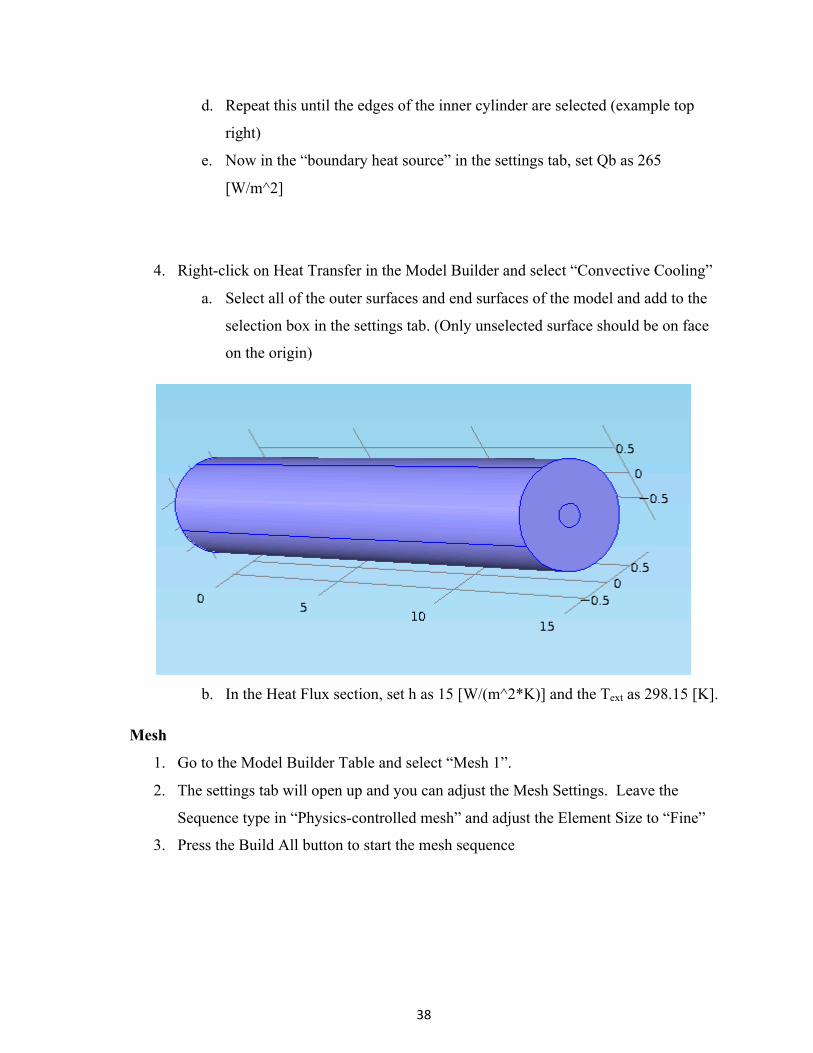
38

d. Repeat this until the edges of the inner cylinder are selected (example top

right)

e. Now in the “boundary heat source” in the settings tab, set Qb as 265

[W/m^2]

4. Right-click on Heat Transfer in the Model Builder and select “Convective Cooling”

a. Select all of the outer surfaces and end surfaces of the model and add to the

selection box in the settings tab. (Only unselected surface should be on face

on the origin)

b. In the Heat Flux section, set h as 15 [W/(m^2*K)] and the Text as 298.15 [K].

Mesh

1. Go to the Model Builder Table and select “Mesh 1”.

2. The settings tab will open up and you can adjust the Mesh Settings. Leave the

Sequence type in “Physics-controlled mesh” and adjust the Element Size to “Fine”

3. Press the Build All button to start the mesh sequence

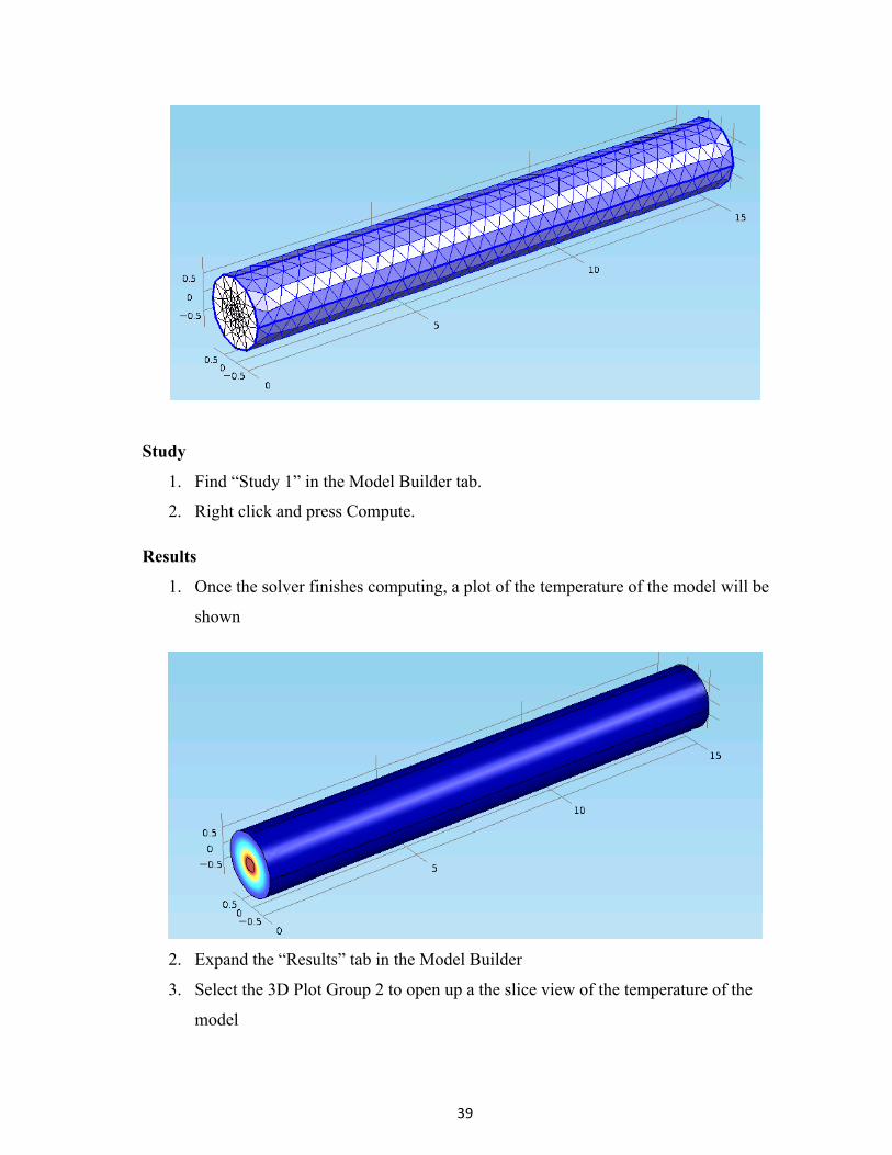
39

Study

1. Find “Study 1” in the Model Builder tab.

2. Right click and press Compute.

Results

1. Once the solver finishes computing, a plot of the temperature of the model will be

shown

2. Expand the “Results” tab in the Model Builder

3. Select the 3D Plot Group 2 to open up a the slice view of the temperature of the

model

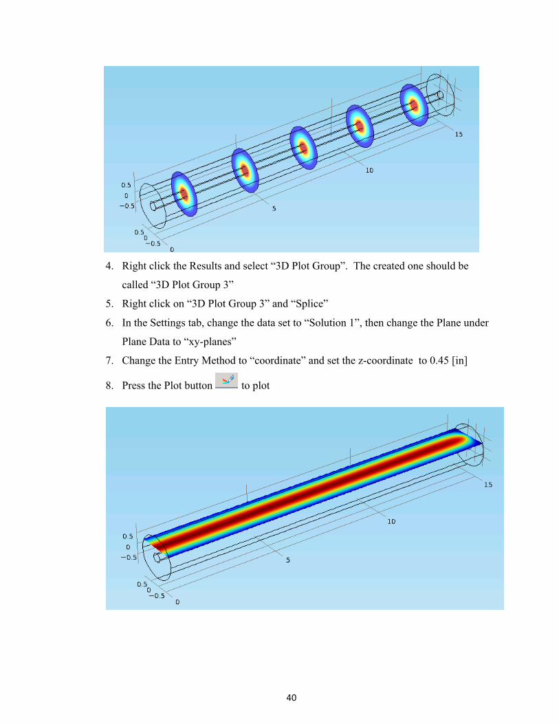
40

4. Right click the Results and select “3D Plot Group”. The created one should be

called “3D Plot Group 3”

5. Right click on “3D Plot Group 3” and “Splice”

6. In the Settings tab, change the data set to “Solution 1”, then change the Plane under

Plane Data to “xy-planes”

7. Change the Entry Method to “coordinate” and set the z-coordinate to 0.45 [in]

8. Press the Plot button to plot

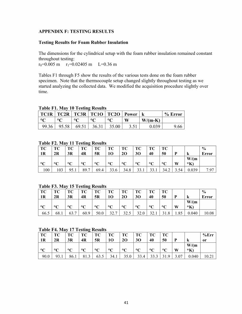
41

APPENDIX F: TESTING RESULTS Testing Results for Foam Rubber Insulation The dimensions for the cylindrical setup with the foam rubber insulation remained constant throughout testing: r0=0.005 m r1=0.02405 m L=0.36 m Tables F1 through F5 show the results of the various tests done on the foam rubber specimen. Note that the thermocouple setup changed slightly throughout testing as we started analyzing the collected data. We modified the acquisition procedure slightly over time. Table F1. May 10 Testing Results TC1R TC2R TC3R TC1O TC2O Power k % Error °C °C °C °C °C W W/(m-K) 99.36 95.58 69.51 36.31 35.00 3.51 0.039 9.66

Table F2. May 11 Testing Results TC 1R

TC 2R

TC 3R

TC 4R

TC 5R

TC 1O

TC 2O

TC 3O

TC 40

TC 50 P k

% Error

°C °C °C °C °C °C °C °C °C °C W W/(m*K)

100 103 95.1 89.7 69.4 33.6 34.8 33.1 33.1 34.2 3.54 0.039 7.97 Table F3. May 15 Testing Results TC 1R

TC 2R

TC 3R

TC 4R

TC 5R

TC 1O

TC 2O

TC 3O

TC 40

TC 50 P k

% Error

°C °C °C °C °C °C °C °C °C °C W W/(m*K)

66.5 68.1 63.7 60.9 50.0 32.7 32.5 32.0 32.1 31.8 1.85 0.040 10.08 Table F4. May 17 Testing Results TC 1R

TC 2R

TC 3R

TC 4R

TC 5R

TC 1O

TC 2O

TC 3O

TC 40

TC 50 P k

%Error

°C °C °C °C °C °C °C °C °C °C W W/(m*K)

90.0 93.1 86.1 81.3 63.5 34.1 35.0 33.4 33.3 31.9 3.07 0.040 10.21

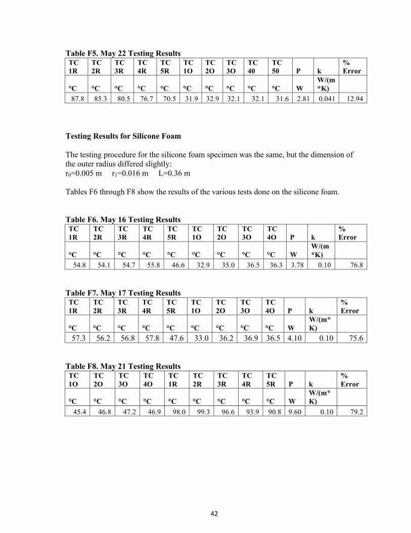
42

Table F5. May 22 Testing Results TC 1R

TC 2R

TC 3R

TC 4R

TC 5R

TC 1O

TC 2O

TC 3O

TC 40

TC 50 P k

% Error

°C °C °C °C °C °C °C °C °C °C W W/(m*K)

87.8 85.3 80.5 76.7 70.5 31.9 32.9 32.1 32.1 31.6 2.81 0.041 12.94 Testing Results for Silicone Foam The testing procedure for the silicone foam specimen was the same, but the dimension of the outer radius differed slightly: r0=0.005 m r1=0.016 m L=0.36 m Tables F6 through F8 show the results of the various tests done on the silicone foam. Table F6. May 16 Testing Results TC 1R

TC 2R

TC 3R

TC 4R

TC 5R

TC 1O

TC 2O

TC 3O

TC 4O P k

% Error

°C °C °C °C °C °C °C °C °C W W/(m*K)

54.8 54.1 54.7 55.8 46.6 32.9 35.0 36.5 36.3 3.78 0.10 76.8 Table F7. May 17 Testing Results TC 1R

TC 2R

TC 3R

TC 4R

TC 5R

TC 1O

TC 2O

TC 3O

TC 4O P k

% Error

°C °C °C °C °C °C °C °C °C W W/(m*K)

57.3 56.2 56.8 57.8 47.6 33.0 36.2 36.9 36.5 4.10 0.10 75.6 Table F8. May 21 Testing Results TC 1O

TC 2O

TC 3O

TC 4O

TC 1R

TC 2R

TC 3R

TC 4R

TC 5R P k

% Error

°C °C °C °C °C °C °C °C °C W W/(m*K)

45.4 46.8 47.2 46.9 98.0 99.3 96.6 93.9 90.8 9.60 0.10 79.2

Documents

Prepared by Alan Guthrie, Michael Hartley, Alex Moon… · Redesigning the ME 331 Heat Conduction Experiment Prepared by Alan Guthrie, Michael Hartley, Alex Moon, and Krista Simonson