Embed Size (px)
Citation preview
AN UNSPLIT STAGGEREDMESH SCHEME FORMULTIDIMENSIONAL
MAGNETOHYDRODYNAMICS WITH EFFICIENT DISSIPATION CONTROLS
Dongwook Leea and Anil Deaneb,∗
aASC FLASH Center, University of Chicago, 5640 S. Ellis, Chicago, IL 60637
bInstitute for Physical Science and Technology, University of Maryland,College Park, MD 20742
– PREPRINT –November 5, 2007
Abstract
We introduce an unsplit staggered mesh scheme (USM) that solves multidimensional magnetohy-drodynamics (MHD) by a constrained transport method with high-order Godunov fluxes, incorporatingthree new developments that enhance performance. The USM scheme handles multidimensional MHDterms, proportional to∇ ·B, in a new directionally unsplit data reconstruction step. This reconstructionstep maintains in-plane dynamics very well, as shown by two-dimensional tests. The scheme uses acompact form of the discrete induction equation and since the accuracy of the computed electric fielddirectly influences the quality of the magnetic field solution, we address the lack of proper dissipativebehavior in previous electric field averaging schemes and present a new modified electric field construc-tion (MEC) that includes multidimensional derivative information and is more accurate. We also obtaina relation between the induction equation and its difference form and use this to derive a set of cor-responding modified equations which show anti-dissipative behavior of cell-face magnetic fields. Wepresent an efficient treatment suppressing the anti-dissipative terms by introducing a difference formula-tion with balancing dissipation control (DC) that maintains the divergence-free property on a staggeredmeshes. We use this difference scheme to highlight important properties that avoid unphysical growthof field variables. Our numerical tests show that numerical instability can occur if the anti-dissipationterms are ignored or otherwise not explicitly controlled. A series of comparison studies demonstratesthe excellent performance of the full USM-MEC-DC scheme for many quite stringent multidimensionalMHD test problems. The scheme is implemented and currently available in the University of ChicagoASC FLASH Center’s FLASH 3 release.
1 Introduction
A well-designed numerical MHD algorithm should generate solutions that reflect the fact that thereare no isolated magnetic monopoles. Brackbill and Barnes (1980) [6] showed that violating the∇ ·B = 0constraint can cause fictitious forces to develop parallel to the magnetic fields. This can result in extra sourceterms in the momentum, induction and energy equations. For instance, the Lorentz force per unit volume(assuming overall charge neutrality) can be written as
j ×B = (∇×B)×B (1)
∗Corresponding author,[email protected].
1
= (B ·∇)B− 12
∇B2 (2)
= ∇ · (BB)− (∇ ·B)B− 12
∇B2, (3)
wherej andB are the current density and magnitude of the magnetic fields. The first and second terms inequation (2) represent the forces from magnetic tension and magnetic pressure, respectively.
From (3), if ∇ ·B 6= 0 the nonzero value of∇ ·B will grow proportionally withB producing an extracompressive magnetic component parallel to the magnetic field and an unphysical magnetic accelerationalong the field lines. Since the gas pressure,
p = (γ−1)(E− 12
ρU2− 12
B2), (4)
whereE,U , andB are the total energy density, magnitudes of velocity fields and magnetic fields respectively,in simulations, nonzero∇ ·B value will increase the magnetic pressure1
2B2 and from (4), the gas pressurepwill correspondingly be reduced relative to the divergence-free case. In many numerical simulations,∇ ·Bis typically small, but not exactly zero, and being a discretization error, the resultant error can accumulateover the computational domain and produce erroneous solutions.
More generally, unphysical growth of the magnetic field in a simulation can lead to negative pressurestates in very lowβ plasma flows in a region where a predictive magnetic pressure exhibits spurious growthrates, which in turn, fails to preserve the physical positivity of gas pressure. On the other hand in very highβ regimes it is also hard to maintain correct plasma flow properties because very weak magnetic fields caneasily be affected at the level of discretization errors. In either case, erroneous magnetic field growth ratesinfluence the energy balance between the thermal and magnetic pressures, potentially changing the topologyof the magnetic fields, affecting the global field configuration and attendant particle propagation.
For these reasons attention has been paid to staggered mesh schemes which naturally avoid these issues.Here we develop a new such discrete formulation for the induction equation which avoids unphysical growthof the magnetic fields, and produces accurate and stable plasma solutions over a wide range of plasmaβ.
1.1 Cell-centered Fields Algorithms in High-Order Godunov MHD
Over the last decade high-order Godunov methods, originally developed in hydrodynamics, have be-come of great interest in MHD because of their accuracy and robustness. A brief list of developmentsincludes the work of Brio and Wu (1988) [8], Zachary, Malagoli, and Colella (1994) [37], Dai and Wood-ward (1994) [11], Powellet al. (1994) [28], Ryu and Jones (1995) [30], Balsara and Spicer (1998) [2],Londrillo and Del Zanna (1999) [24], Penet al. (2003) [27], Londrillo and Del Zanna (2004) [25], Balsara(2003) [4], Crockettet al. (2005) [10], and Gardiner and Stone (2005) [17].
The high-order Godunov scheme, first developed by van Leer (1979) for Euler flows has thereafteropened a new era of robust and accurate performance in numerical simulations of MHD as well as hydro-dynamics. Early efforts in high-order Godunov MHD schemes focused entirely on numerical formulationsthat collocated the magnetic fields at cell centers because the underlying aspects of Godunov algorithms arebased on conservation laws in which the cell-centered variables are conserved. Thus the MHD equationswere treated as a straightforward system of conservation laws in earlier Godunov formulations.
In formulations with cell-centered fields there is no particular difficulty encountered except in multidi-mensions. This is because in one-dimensional MHD the normal field is held constant and divergence-lessevolution of the magnetic fields is obtained naturally. In multidimensional MHD, however, the requirementof maintaining the solenoidal constraint involves solving the induction equation, which for ideal MHD hasthe form,
∂B∂t
+∇×E = 0. (5)
2
Taking the divergence of the induction equation (5) gives,
∂∇ ·B∂t
= ∇ · (−∇×E) = 0, (6)
and we see that the induction equation implies the divergence-less evolution of the magnetic fields. Thisanalytical result may not hold true numerically, because the discrete divergence of the discrete curl may notgive zero identically.
Until recently, two traditional approaches have been proposed to enforce the divergence-free constraintin formulations using cell-centered fields. The first is the projection method, proposed by Brackbill andBarnes in the context of MHD[6] (see also early works cited in [1,30,37] and recently in [10]), which takesa divergence-cleaning step in their high-order Godunov based MHD scheme. In this approach two choicesare available, a scalar or vector divergence-cleaning, depending on the choice of real or Fourier spaces inwhich the divergence-cleaning is performed. The disadvantage of the approach is the cost of the associatedPoisson equation solution by either direct or iterative methods. In addition to the computational expensive,the projection methods has restrictions on types of boundary conditions and associated difficulties on non-Cartesian domains. On a parallel or distributed computer, since the method requires a global solution to aPoisson equation, there is an additional coding burden and cost of all-to-all communication. Yet anotherdisadvantage is extra complexity because the discretization of the elliptic equation must be compatible withthat of the MHD equations. An adaptive mesh refinement (AMR) scheme can be implemented in the scalardivergence-cleaning approach, but become progressively computationally expensive as the AMR hierarchyincreases in the Poisson solve. The situation is even more acute for implementing a vector divergence-cleaning approach for an AMR algorithm. For more details on these and other numerical issues for thisapproach see [5,35].
The second method, the so-called 8-wave formalism, proposed by Powellet al. [29], utilizes the modi-fied MHD equations that explicitly includes source terms proportional to∇ ·B. An additional eighth wavereflects the propagation of the magnetic monopole ”field,” designed to be convected with local flow speeds,and eventually advected out of the computational domain. Although the scheme is found to be robust andaccurate (as compared to the basic conservative scheme), this results in a non-conservative form of the MHDgoverning equations and is susceptible to producing incorrect jump conditions and propagation speeds acrossdiscontinuities in certain problems [29, 35]. Because of its inherent formalism allowing a truncation errorof ∇ ·B this scheme lacks the divergence-free property and can potentially fail to capture correct magneticfield topologies. There have also been other approaches [13, 20] to extend 8-wave schemes that manifest∇ ·B as a source term.
1.2 Cell Face-centered Fields Algorithms in High-Order Godunov MHD: the StaggeredMesh Algorithm
To overcome issues raised in formulating high-order Godunov based MHD using cell-centered fields,researchers have developed various staggered mesh algorithms that use a staggered collocation of the mag-netic field and solve the induction equation (5) via a discrete form of Stokes’ Theorem.
The staggered mesh algorithm, first introduced by Yee (1966) [36] to compute divergence-free MHDflows in a finite difference formulation that transports the electromagnetic fields, has resulted in numerousapproaches. Bretchtet al. (1981) [7] used a staggered mesh formulation for their global MHD modeling ofEarth’s magnetosphere for which they used a non-linear FCT flux limiter. Evans and Hawley 15] followeda vector potential approach on a staggered grid for evolution of the MHD induction equation. Another ap-proach by DeVore (1991) [14] also used the staggered mesh arrangement and applied it using a flux correctedtransport (FCT) algorithm. Following Evans and Hawley (1988) [15], the termconstrained transport(CT)has become popular and encompasses all the various methods developed with a staggered mesh approache
3
[2,4,12,14,15,17,24,31,35]. The original CT method placed the surface variables – the components of themagnetic field – at the cell face centers (cell-faces), and the rest of the volumetric variables such as mass,momentum and energy at the cell-centers on a staggered grid. A variant CT approach by Toth [35] placedall of the variables at the cell centers and used central differencing for the induction equation. Toth alsomade an extensive comparative study of different MHD schemes focusing on the divergence-free propertyof each scheme. and compared various approaches differing in how the base scheme (e.g.van Leer’s TVD-MUSCL, or Yee’s TVD-Lax Friedrich) is modified with regard to the induction equation. Toth’s study notonly compared three major algorithms (e.g. projection schemes, 8-wave schemes, and CT based staggeredmesh schemes) but also different approaches within the CT formulation.
In CT schemes, different approaches are adopted in obtaining the electric field,E = −u×B (in idealMHD). Theflux-CT scheme of Balsara and Spicer [2] uses second-order Godunov fluxes to constructE byusing the so-called duality relationship between the components of the flux vector and the electric fields.Thefield-interpolatedCT scheme of Dai and Woodward [12] uses interpolated magnetic and velocity fieldsto obtain the electric field in their Godunov-type formulation. Ryuet al. [31] also proposed atransport-flux-interpolatedCT scheme which basically transports the upwind fluxes along with the upwind correction termsfor maintaining the TVD property. Balsara studied [3, 4] a new reconstruction algorithm for cell-centeredmagnetic fields. In thismodified-CT approach the magnetic fields at each cell center are reconstructed di-rectly from divergence-free cell-face field components using a reconstruction polynomial. By design suchreconstructed magnetic fields at the cell centers (and not only the cell-face fields) are also guaranteed tomaintain the divergence-free constraint. Recently, Gardiner and Stone [17] have developed a multidimen-sional CT scheme that is consistent with plane-parallel, grid-aligned one-dimensional base flow problemsby modifying the simple arithmetic electric field averaging scheme of Balsara and Spicer [2]. Another ap-proach,upwinding-CT (UTC) scheme, was proposed by Londrillo and Del Zanna [25]. Their approach useda similar reconstruction algorithm as in [3,4] for the magnetic field and evaluates the electric field based onan upwinding strategy in their Godunov-type scheme. In the UTC scheme, the divergence-free property ismaintained intrinsically. Yet it is evident from their test results that the scheme suffers from keeping∇ ·Bonly approximately low, allowing values up to an order of 10−4 (See [24]), while, as shown later the schemepresented here preserves∇ ·B to the order of 10−12−10−16 in simulations. It is worth mentioning that, inToth’s work [35], one of the most accurate high-order MHD schemes is the flux-CT scheme of Balsara andSpicer [2]. Balsara [3, 4] has also extended his original flux-CT scheme and implemented it on an AMRgrid.
In developing our scheme we adopt the flux-CT approach of [2] and extend its basic ideas to develop anew unsplit staggered mesh scheme. Upon systematically developing a modified electric field construction(MEC) and dissipation control (DC) we term our complete schemes USM-MEC-DC.
The paper is organized as follows. In Section 2, we first introduce a new second-order MUSCL-Hancocktype data reconstruction scheme using a single step characteristic tracing formalism. This step includesmultidimensional MHD terms important in nonlinear evolutionary plasma flows. The data reconstructionstep is followed by solving a Riemann problem that produces high-order Godunov fluxes. Using thesefluxes, in Section 3, we present a new modified electric field construction (MEC) algorithm that extendsthe basic construction scheme of Balsara and Spicer [2] to a scheme containing multidimensional gradientinformation. In Section 4, we examine a discrete form of the induction equation that has been used inCT-type schemes and its address anti-dissipative properties by studying associated modified equations. Weuse this relationship to present a new discrete formulation that controls anti-dissipation and also ensures thedivergence-free constraint. In Section 5 we present results of various test problems that demonstrate thesignificant quantitative and qualitative performance of our scheme. We conclude the paper in Section 6.
4
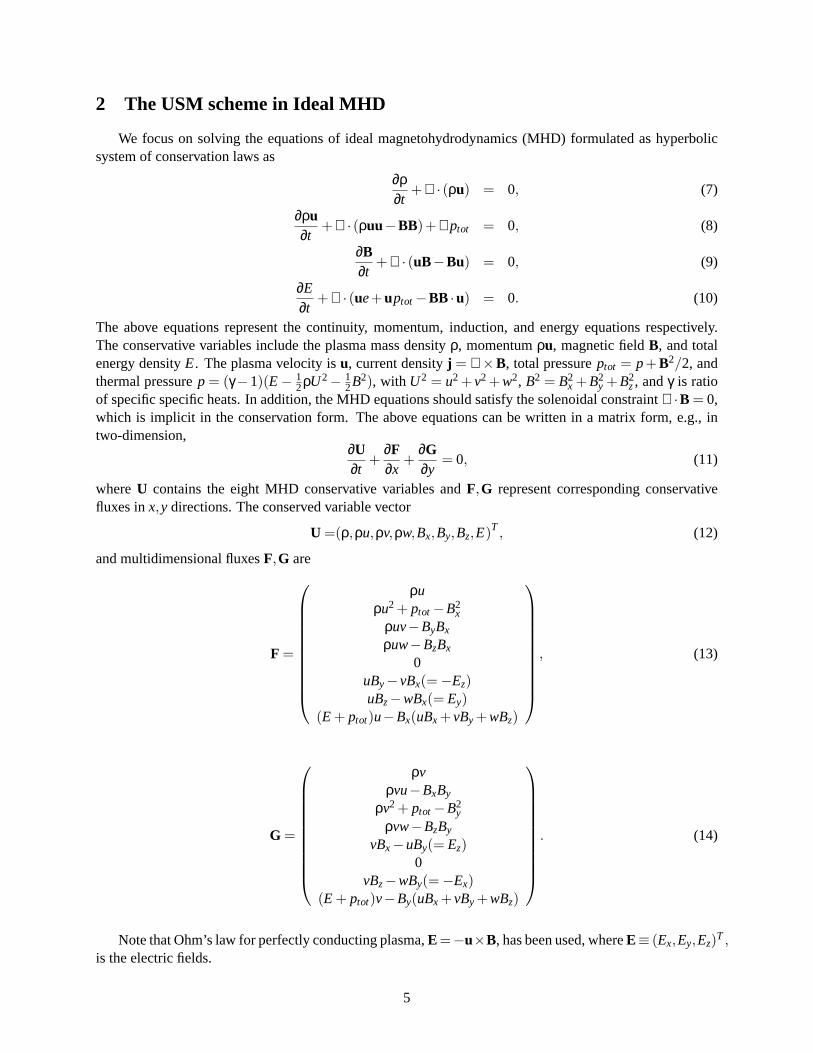
2 The USM scheme in Ideal MHD
We focus on solving the equations of ideal magnetohydrodynamics (MHD) formulated as hyperbolicsystem of conservation laws as
∂ρ∂t
+∇ · (ρu) = 0, (7)
∂ρu∂t
+∇ · (ρuu−BB)+∇ptot = 0, (8)
∂B∂t
+∇ · (uB−Bu) = 0, (9)
∂E∂t
+∇ · (ue+uptot−BB ·u) = 0. (10)
The above equations represent the continuity, momentum, induction, and energy equations respectively.The conservative variables include the plasma mass densityρ, momentumρu, magnetic fieldB, and totalenergy densityE. The plasma velocity isu, current densityj = ∇×B, total pressureptot = p+B2/2, andthermal pressurep = (γ−1)(E− 1
2ρU2− 12B2), with U2 = u2 +v2 +w2, B2 = B2
x +B2y +B2
z, andγ is ratioof specific specific heats. In addition, the MHD equations should satisfy the solenoidal constraint∇ ·B = 0,which is implicit in the conservation form. The above equations can be written in a matrix form, e.g., intwo-dimension,
∂U∂t
+∂F∂x
+∂G∂y
= 0, (11)
whereU contains the eight MHD conservative variables andF,G represent corresponding conservativefluxes inx,y directions. The conserved variable vector
U =(ρ,ρu,ρv,ρw,Bx,By,Bz,E)T , (12)
and multidimensional fluxesF,G are
F =
ρuρu2 + ptot−B2
xρuv−ByBx
ρuw−BzBx
0uBy−vBx(=−Ez)uBz−wBx(= Ey)
(E + ptot)u−Bx(uBx +vBy +wBz)
, (13)
G =
ρvρvu−BxBy
ρv2 + ptot−B2y
ρvw−BzBy
vBx−uBy(= Ez)0
vBz−wBy(=−Ex)(E + ptot)v−By(uBx +vBy +wBz)
. (14)
Note that Ohm’s law for perfectly conducting plasma,E =−u×B, has been used, whereE≡ (Ex,Ey,Ez)T ,is the electric fields.
5
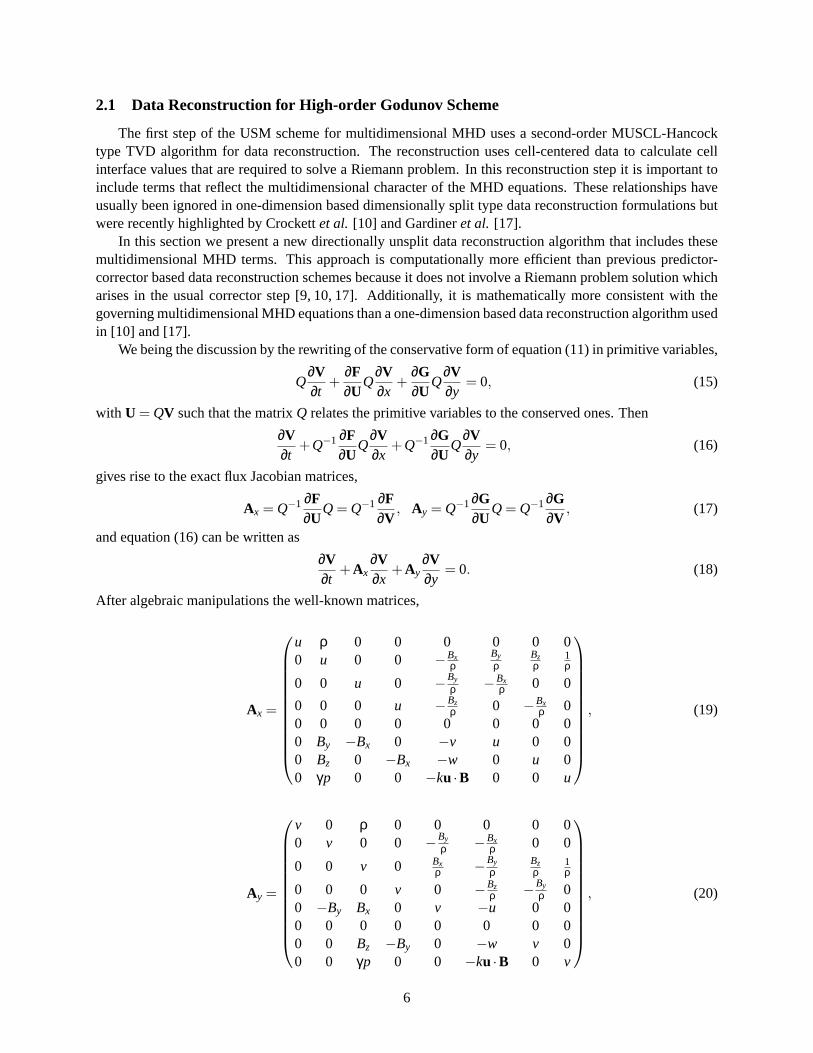
2.1 Data Reconstruction for High-order Godunov Scheme
The first step of the USM scheme for multidimensional MHD uses a second-order MUSCL-Hancocktype TVD algorithm for data reconstruction. The reconstruction uses cell-centered data to calculate cellinterface values that are required to solve a Riemann problem. In this reconstruction step it is important toinclude terms that reflect the multidimensional character of the MHD equations. These relationships haveusually been ignored in one-dimension based dimensionally split type data reconstruction formulations butwere recently highlighted by Crockettet al. [10] and Gardineret al. [17].
In this section we present a new directionally unsplit data reconstruction algorithm that includes thesemultidimensional MHD terms. This approach is computationally more efficient than previous predictor-corrector based data reconstruction schemes because it does not involve a Riemann problem solution whicharises in the usual corrector step [9, 10, 17]. Additionally, it is mathematically more consistent with thegoverning multidimensional MHD equations than a one-dimension based data reconstruction algorithm usedin [10] and [17].
We being the discussion by the rewriting of the conservative form of equation (11) in primitive variables,
Q∂V∂t
+∂F∂U
Q∂V∂x
+∂G∂U
Q∂V∂y
= 0, (15)
with U = QV such that the matrixQ relates the primitive variables to the conserved ones. Then
∂V∂t
+Q−1 ∂F∂U
Q∂V∂x
+Q−1 ∂G∂U
Q∂V∂y
= 0, (16)
gives rise to the exact flux Jacobian matrices,
Ax = Q−1 ∂F∂U
Q = Q−1 ∂F∂V
, Ay = Q−1 ∂G∂U
Q = Q−1 ∂G∂V
, (17)
and equation (16) can be written as
∂V∂t
+Ax∂V∂x
+Ay∂V∂y
= 0. (18)
After algebraic manipulations the well-known matrices,
Ax =
u ρ 0 0 0 0 0 00 u 0 0 −Bx
ρBy
ρBzρ
1ρ
0 0 u 0 −By
ρ −Bxρ 0 0
0 0 0 u −Bzρ 0 −Bx
ρ 00 0 0 0 0 0 0 00 By −Bx 0 −v u 0 00 Bz 0 −Bx −w 0 u 00 γp 0 0 −ku ·B 0 0 u
, (19)
Ay =
v 0 ρ 0 0 0 0 00 v 0 0 −By
ρ −Bxρ 0 0
0 0 v 0 Bxρ −By
ρBzρ
1ρ
0 0 0 v 0 −Bzρ −By
ρ 00 −By Bx 0 v −u 0 00 0 0 0 0 0 0 00 0 Bz −By 0 −w v 00 0 γp 0 0 −ku ·B 0 v
, (20)
6
are obtained, wherek = 1− γ. Note that, from relations (13) and (14), there are seven non-trivial equationsand one trivial equation for which the time derivative becomes zero. This yields the zeros located in eachcorresponding row in the above 8×8 matrices (19) and (20). In general, the primitive form of the equationscan be replaced by a quasi-linear system of equations,
∂V∂t
+ A ·∇V =∂V∂t
+(Ax, Ay) ·∇V = 0, (21)
whereA ≡ A(V) = A(VL,VR) with left and right states,VL,VR, assuming these and the solution are closeto a constant state,V.
In one-dimensional MHD the full eight set of MHD equations can be reduced to seven. Should thegradient of the normal magnetic field be zero, such a constant normal field is not to be evaluated. Formultidimensional MHD, however, the terms∂Bx/∂x and∂By/∂y do not vanish in general, and play crucialroles that cannot be ignored. Dimensional splitting based on a one-dimensional MHD system of equationslacks these gradient terms and can produce incorrect solutions.
In order to include the gradient terms for multidimensional MHD in a data reconstruction fomulation, wepresent an approach which is built upon a directionally unsplit second-order MUSCL-Hancock algorithm.We treat the evolution of the normal field,BN, separately from the other primitive variables, i.e., for a casewith BN = Bx, define
V =[
VBx
]andAx =
[Ax ABx
0 0
]. (22)
HereV is a 7×1 vector excludingBx, Ax is a 7×7 matrix omitting both the fifth row and column in theoriginal matrixAx (19), andABx is a 7×1 vector,
ABx =[0,−Bx
ρ,−
By
ρ,−Bz
ρ,−v,−w,−ku ·B
]T
. (23)
Similarly, for BN = By, Ay is constructed by omitting both the sixth row and column in the original matrixAy (20), andABy is
ABy =[0,−Bx
ρ,−
By
ρ,−Bz
ρ,−u,−w,−ku ·B
]T
. (24)
A similar approach was adopted by Crockettet al. [10] but their equivalent terms forAx andAy omittedthe factork in the last entry. The termsABx andABy will be referred to as multidimensional MHD termsin the following. Note that the hat (ˆ) notation has been introduced for the reduced system (i.e., the onecorresponding to the usual one-dimensional MHD equation) and the bar (-) notation retained for the re-assembled full system.
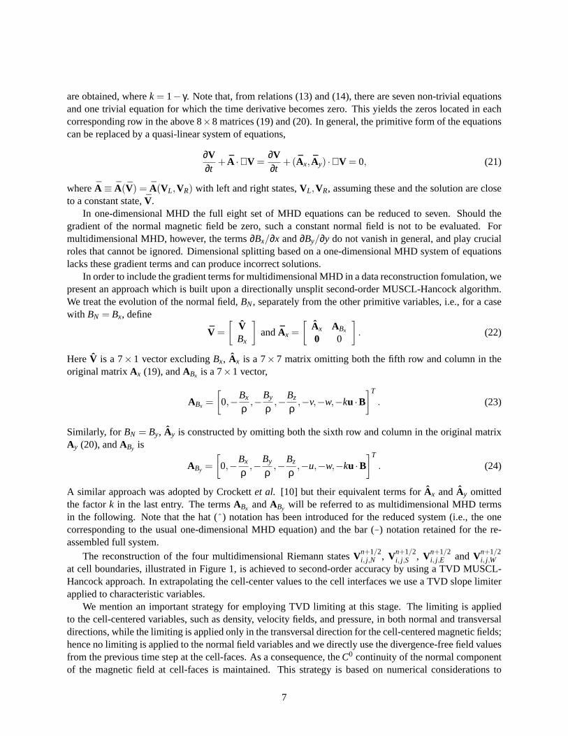
The reconstruction of the four multidimensional Riemann statesVn+1/2i, j,N , Vn+1/2
i, j,S , Vn+1/2i, j,E andVn+1/2
i, j,Wat cell boundaries, illustrated in Figure 1, is achieved to second-order accuracy by using a TVD MUSCL-Hancock approach. In extrapolating the cell-center values to the cell interfaces we use a TVD slope limiterapplied to characteristic variables.
We mention an important strategy for employing TVD limiting at this stage. The limiting is appliedto the cell-centered variables, such as density, velocity fields, and pressure, in both normal and transversaldirections, while the limiting is applied only in the transversal direction for the cell-centered magnetic fields;hence no limiting is applied to the normal field variables and we directly use the divergence-free field valuesfrom the previous time step at the cell-faces. As a consequence, theC0 continuity of the normal componentof the magnetic field at cell-faces is maintained. This strategy is based on numerical considerations to
7
prevent undesirable jumps in the normal components of the fields at the cell boundaries. Indeed, Powellet al. [28] noticed that if the normal fields have jumps at the cell boundaries, the resultant cell-centeredfield based MHD formulation using a Riemann solver becomes ill-defined. They eventually resolved this byintroducing the 8-wave model with modified MHD equations.
In the current scheme using divergence-free cell face-centered fields the continuity consideration of thenormal fields at the cell interfaces is thus met straightforwardly.
∗(i, j)
Vn+1/2i, j−1,N
Vn+1/2i, j,S
Vn+1/2i, j,N
Vn+1/2i, j+1,S
Vn+1/2i−1, j,E Vn+1/2
i, j,W Vn+1/2i, j,E Vn+1/2
i+1, j,W
Figure 1: The boundary extrapolated values on a 2D cell geometry. The values are subscripted byN,S,EandW accordingly. These are used as the state values for solving Riemann problem at each cell boundaryinterface.
Given the quasi-linearized MHD equations,
Vn+1/2i, j,E,W = Vn
i, j +12[±I − ∆t
∆xAx(Vn
i, j)]∆ni −
∆t2∆y
Ay(Vni, j)∆
nj , (25)
Vn+1/2i, j,N,S = Vn
i, j −∆t
2∆xAx(Vn
i, j)∆ni +
12[±I − ∆t
∆yAy(Vn
i, j)]∆nj , (26)
where the plus and minus signs correspond to directions ofN,E andS,W respectively, andAx(Vni, j), Ax(Vn
i, j)represent matrices calculated atVn
i, j , we first consider data reconstruction in the normal direction (e.g., thefirst two terms in the left hand side of (25)),[
VBx
]n+1/2,‖
i, j,E,W
=[
VBx
]n
i, j
+12
(±[
I 00 1
]− ∆t
∆x
[Ax ABx
0 0
]n
i, j
)∆n
i , (27)
where∆ni =
(∆n
i ,∆Bnx,i
)Tand∆Bn
x,i = bnx,i+1/2, j −bn
x,i−1/2, j (the meaning of∆ni becoming clear shortly). The
notationBτ andbτ denote cell-centered and cell-face magnetic field components respectively, withτ = x,y,z.In the staggered mesh CT algorithm,∆Bn
x,i is constructed such that the numerical divergence is zero usingthe cell-centered magnetic fields. In other words,∆Bn
x,i and∆Bny, j are chosen such that
∆Bnx,i
∆x+
∆Bny, j
∆y= 0, (28)
8
where we analogously define∆Bny, j = bn
y,i, j+1/2−bny,i, j−1/2. As noted previously no TVD limiting is applied
to ∆Bnx,i or ∆Bn
y, j . Solving (27) is equivalent to considering two subsystems Vn+1/2,‖i, j,E,W = Vn
i, j +12
(±I − ∆t
∆xAx
)n
i, j∆n
i − ∆t2∆x(ABx)
ni, j∆Bn
x,i ,
(Bx)n+1/2,‖i, j,E,W = Bn
x,i, j ± 12∆Bn
x,i .(29)
where the second relation in (29) becomes
(Bx)n+1/2,‖i, j,E,W = Bn
x,i, j ±12
∆Bnx,i = bn
x,i±1/2, j , (30)
when the cell-centered magnetic field is reconstructed as
Bnx,i, j =
12
(bn
x,i+1/2, j +bnx,i−1/2, j
). (31)
We apply the eigenstructure of the one-dimensional based MHD equations and use characteristic tracingfor the first two terms in the first equation in (29). Applying characteristic tracing results in
Vn+1/2,‖i, j,W = Vn
i, j +12 ∑
k;λki, j<0
(−1− ∆t
∆xλk
i, j
)r k
x,i, j ∆αni −
∆t2∆x
(ABx)ni, j∆Bn
x,i , (32)
Vn+1/2,‖i, j,E = Vn
i, j +12 ∑
k;λki, j>0
(1− ∆t
∆xλk
i, j
)r k
x,i, j ∆αnj −
∆t2∆x
(ABx)ni, j∆Bn
x,i , (33)
with characteristic limiting in the normal direction,
∆αni = TVD_Limiter
[lkx,i, j · ∆n
i,+, lkx,i, j · ∆ni,−
]. (34)
Hereλkx,i, j , r
kx,i, j , l
kx,i, j represent the eigenvalue, and the right and left eigenvectors ofAx, calculated at the
corresponding cell center(i, j) in thex-direction at time stepn, and∆ni,+ = Vn
i+1, j − Vni, j , ∆n
i,− = Vni, j − Vn
i−1, j
(similarly for ∆nj,±).
The next step includes the transversal flux contribution to the calculated normal state variables. Thistransversal step, using the eigenstructure of the MHD equations, completes the update from the transversalflux contributions, e.g., the third and second terms in (25) and (26), respectively. For instance, in (25) thetransversal step can be updated as
Vn+1/2i, j,E,W = Vn+1/2,‖
i, j,E,W − ∆t2∆y
Ay(Vni, j)∆
nj . (35)
Again, this can be written as[VBy
]n+1/2
i, j,E,W
=[
VBy
]n+1/2,‖
i, j,E,W
− ∆t2∆y
[Ay ABy
0 0
]n
i, j
∆nj . (36)
This reduces to solving just one subsystem,
Vn+1/2i, j,E,W = Vn+1/2,‖
i, j,E,W − ∆t2∆y
(Ay)ni, j ∆
nj −
∆t2∆y
(ABy)ni, j∆Bn
y, j . (37)
9
Using the eigensystem at the cell center (i, j) in they-direction, we get,
Vn+1/2i, j,E,W = Vn+1/2,‖
i, j,E,W − ∆t2∆y
7
∑k=1
λky,i, j r
ky,i, j ∆αn
j −∆t
2∆y(ABy)
ni, j∆Bn
y, j , (38)
where∆αn
j = TVD_Limiter[lky,i, j · ∆n
j,+, lky,i, j · ∆nj,−
]. (39)
Thus, the four Riemann statesVn+1/2i, j,N ,Vn+1/2
i, j,S ,Vn+1/2i, j,E and Vn+1/2
i, j,W are obtained for each cell. At this
stage, however, it should be noticed that upon taking the transversal steps (e.g., in (38)) theC0 continuity ofthe normal fields at the cell boundaries imposed in the second equation of the normal steps (e.g., (29) and(30)) have been lost. Maintaining this continuity requirement of the normal fields at the boundaries has beenpreviously recognized as an important issue in the MHD Riemann problem[4, 10, 17]. This requirement isessential for physical consistency when solving the MHD Riemann problem. Computationally, allowingjumps in the normal fields at the cell boundaries can lead to more diffusive solutions to Riemann problemsstemming from the upwinding procedure in the Riemann solvers. For the transversal components of themagnetic field, however, discontinuities are allowed and mediate the proper upwinding for them. As a laststep, therefore, it is desirable to enforce the continuity of the normal field components at the cell faces, basedon the relationship in equation (30). This leads to
Bn+1/2x,i, j,E = bn
x,i+1/2, j , Bn+1/2x,i, j,W = bn
x,i−1/2, j , (40)
Bn+1/2y,i, j,N = bn
y,i, j+1/2, Bn+1/2y,i, j,S = bn
y,i, j−1/2. (41)
The algorithm for our Riemann state data reconstruction is based on the method of multidimensionalcharacteristic analysis that can be achieved in one single step, without solving any Riemann problem fortransversal step. Other recent approaches to obtain second-order accurate approximations of the transversalflux derivatives can be found in [9, 10]. There the transversal updating step used the normal predictor stepvalues to solve another set of two intermediate Riemann problems. The resulting interface fluxes werethen used to take numerical derivatives, completing the construction of the second-order Riemann states forevaluating the multidimensional Riemann states.
The current data reconstruction method, which accommodates the MHD eigenstructure multidimen-sionally in a single step, is simpler and computationally less expensive than the previous approach whichuses an extra Riemann solve to evaluate the transversal fluxes. This approach causes no loss of stabilityfor appropriately chosen Courant numbers. The characteristic method is mathematically consistent with thequasi-linearized system of MHD equations.
Another desirable aspect of the current approach can be seen in that the multidimensional termsABx
andABy are included such that they are proportional to∆Bx,i/∆x and∆By, j/∆y. These derivatives are com-puted using the cell-face magnetic fields that are divergence-free from the CT-type formulation of the USMscheme. This implies that the quantitiesu,v,w,Bz, p are all evolved proportional to the sum∆Bx,i
∆x + ∆By, j
∆y ,which is maintained to be zero numerically (see equation (28)). As a result, this dependence has an impor-tant meaning: if perturbations to the divergence∆Bx,i
∆x + ∆By, j
∆y were to be introduced, such perturbation wouldaffect the behavior of all ofu,v,w,Bz, p. For example, as noted by Gardineret al. [17], maintaining planardynamics in two-dimensional MHD problems and not allowing erroneous growth of theBz component isdirectly dependent on how the terms∆Bx,i/∆x and∆By, j/∆y are handled in the data reconstruction step. Inthe current multidimensional predictor-corrector algorithm such growth inBz is avoided, and its success isillustrated in the in-plane field loop advection test problem of Section 5.
The use of the transversal Godunov flux as in [10] can potentially yield incorrect results. Although[10] used similar multidimensional termsABx∆Bn
x,i/∆x for computingE,W normal states andABy∆Bny, j/∆y
10
for N,S normal states, the other set of the multidimensional terms,ABy∆Bny, j/∆y (for E,W states) and
ABx∆Bnx,i/∆x (for N,Sstates), are not included in the transversal directions; instead the numerical derivative
of the transversal fluxes is included. Updating such transversal fluxes can be somewhat similar to includingABy∆Bn
y, j/∆y (for E,W states) andABx∆Bnx,i/∆x (for N,Sstates), but the transversal fluxes and the multidi-
mensional terms in the normal directions are not canceled identically to ensure the divergence-free property.Now that the second-order accurate Riemann states,Vn+1/2
i, j,N,S,E,W, are available second-order Godunovfluxes can be evaluated by solving Riemann problems (RP for short) at cell interfaces. That is,
F∗,n+1/2i−1/2, j = RP
(Vn+1/2
i−1, j,E,Vn+1/2i, j,W
), F∗,n+1/2
i+1/2, j = RP(
Vn+1/2i, j,E ,Vn+1/2
i+1, j,W
), (42)
andG∗,n+1/2
i, j−1/2 = RP(
Vn+1/2i, j−1,N,Vn+1/2
i, j,S
), G∗,n+1/2
i, j+1/2 = RP(
Vn+1/2i, j,N ,Vn+1/2
i, j+1,S
). (43)
2.2 The USM Cell-centered Solution Update
The algorithm updates the cell-centered conserved variables at time stepn+ 1 using an unsplit singlestep,
Un+1i, j = Un
i, j −∆t∆x
{F∗,n+1/2
i+1/2, j −F∗,n+1/2i−1/2, j
}− ∆t
∆y
{G∗,n+1/2
i, j+1/2 −G∗,n+1/2i, j−1/2
}. (44)
In general, after this update, non-zero divergence magnetic fields are still present at cell centers. In thefollowing two sections we describe a new modified electric field construction (MEC) scheme and an efficientdissipation control (DC) algorithm for the discrete induction equation that keep the cell-face magnetic fieldsdivergence-free numerically.
The choice of a time step∆t for our unsplit scheme is limited by the CFL condition, (in 2D),
∆t(∣∣∣λmax
x,i, j
∣∣∣∆x
+
∣∣∣λmaxy,i, j
∣∣∣∆y
)< c. (45)
We use a CFL number ofc = 0.5 for all calculations, except where otherwise noted.
3 Construction of Electric Fields
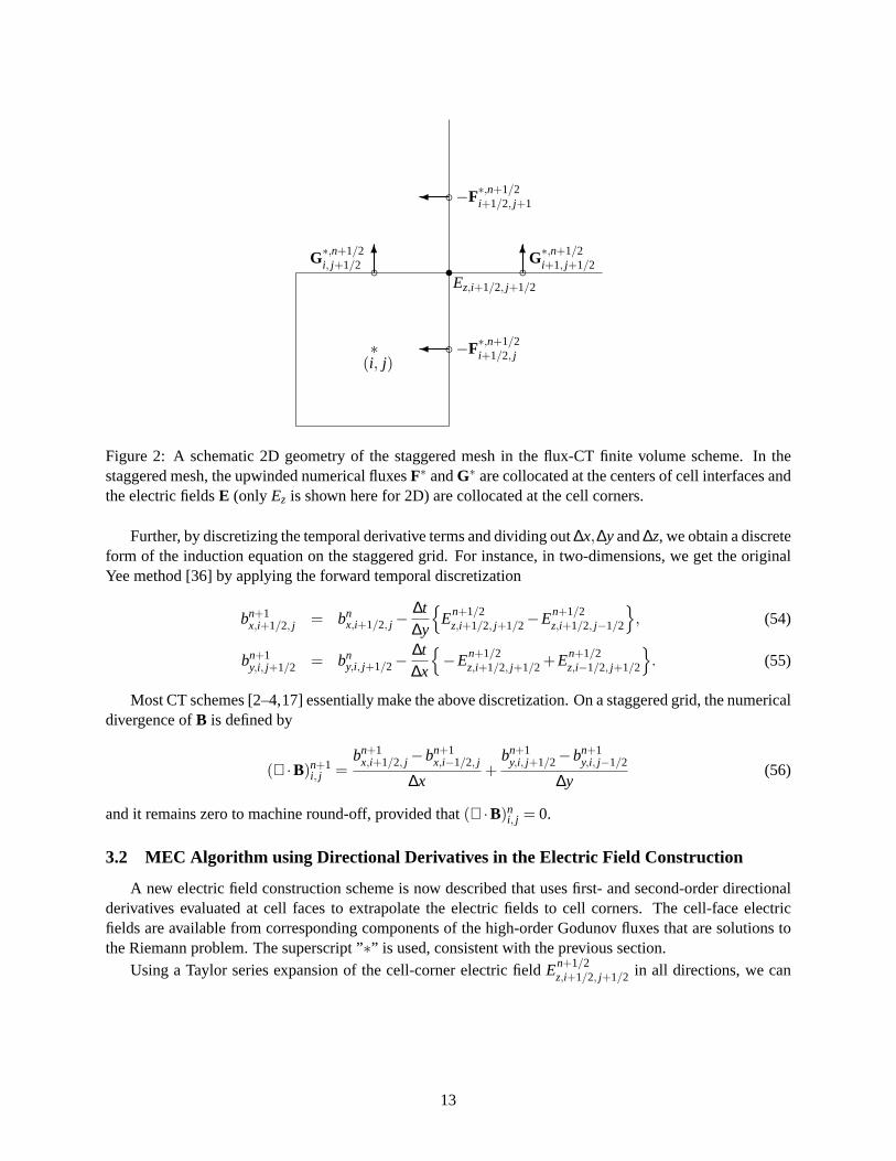
A new modified electric field construction (MEC) scheme that demonstrates full directional informationis introduced and studied in this section. The MEC scheme is obtained by using the second-order accurateGodunov fluxes that are available in staggered mesh schemes (see [2]). Taylor expansions are applied to theflux components of the magnetic fields (or electric fields by the duality relationship [2]) at the face centers toobtain interpolations at each cell corners , where the electric fields are collocated on a staggered grid. Theseelectric fields are then used in the discrete induction equations to evolve divergenceless magnetic fields atcell-faces.
3.1 Electric Field Averaging Scheme
As already mentioned the CT based scheme requires the evaluation of the electric fieldE. Balsara andSpicer [2] proposed to evaluate the electric field on a staggered mesh using high-order Godunov fluxes.There the original arithmetic averaging scheme for the cell-corner (cell edges in three-dimensions) electricfield values, uses the duality relationship between the high-order Godunov flux components for magneticfields and the electric fields. For instance, the negative of the sixth component of the flux inx (equation (13))and the positive of the fifth component of the flux iny (equation (14)) can be interpreted as thezcomponent
11
of the electric fields,Ez, at the cell face centers on the staggered grid. Their proposed way to constructEz ateach cell corner was by taking a spatial average directly from this duality relationship through
En+1/2z,i+1/2, j+1/2 =
14
{−F∗,n+1/2
6,i+1/2, j −F∗,n+1/26,i+1/2, j+1 +G∗,n+1/2
5,i, j+1/2 +G∗,n+1/25,i+1, j+1/2
}=
14
{E∗,n+1/2
z,i+1/2, j +E∗,n+1/2z,i+1/2, j+1 +E∗,n+1/2
z,i, j+1/2 +E∗,n+1/2z,i+1, j+1/2
}, (46)
where the subscripts 6 and 5 denote the sixth and fifth components in the corresponding flux vectors inequations (13)–(14), and the superscript∗ denotes the fluxes (or flux components) directly from the high-order Godunov schemes. See Figure 2 for the staggered mesh arrangement in two-dimensions.
The electric fieldEz in equation (46) can be used to update the induction equation in an appropriatediscretization in different MHD solvers. To discretize the induction equation in a more general sense, weconsider integrating the differential form (5) over a single three-dimensional control volume[i− 1
2, i + 12]×
[ j− 12, j + 1
2]× [k− 12,k+ 1
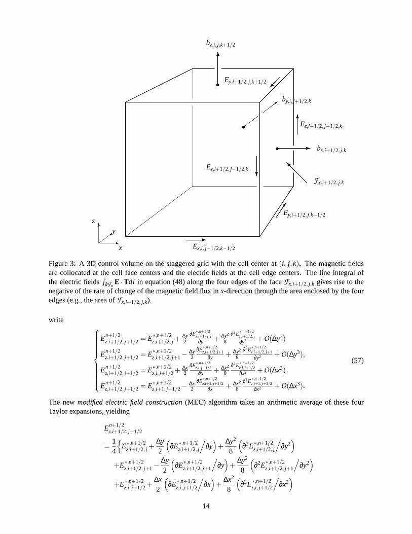
2] in a Cartesian staggered grid (see Figure 3). Taking a surface integral yields
∂∂t
Z Z∑` F`
B ·ndA+Z Z
∑` F`
∇×E ·ndA= 0, (47)
wheren is a unit normal vector and the summation is taken over the six bounding facesF`, ` = 1, . . . ,6.Then for each faceF` of the control volume, applying Stokes’ Theorem, we get
∂∂t
Z ZF`
B ·ndA = −Z Z
F`
∇×E ·ndA
= −Z
∂F`
E ·Tdl (48)
whereT is a unit tangential vector anddl is a line element. Considering the associated normal (denoted byη) and tangential (denoted byτ) components of the magnetic and electric fields for each faceF`, we let
bnη =
1µ(F`)
Z ZF`
BηdA, (49)
En+1/2τ =
1µ(∂F`)
Z∂F`
Eτdl, (50)
whereµ is the Lebesgue measure andη,τ = x,y,z. Note that in the CT formulation the magnetic fieldcomponentsbn
η are the area-averaged values at cell faces, whereas the rest of the conservative variables suchas density, momentum, and energy are volume-averaged quantities.
Using (49) and (50) it is straightforward to rewrite the above equation (48) at each control volume’s facein component-wise form as
∆y∆z∂∂t
bnx,i± 1
2 , j,k
=−{∆z(En+1/2z,i± 1
2 , j+ 12 ,k−En+1/2
z,i± 12 , j− 1
2 ,k)+∆y(En+1/2
y,i± 12 , j,k− 1
2−En+1/2
y,i± 12 , j,k+ 1
2)}, (51)
∆x∆z∂∂t
bny,i, j± 1
2 ,k
=−{∆z(En+1/2z,i− 1
2 , j± 12 ,k−En+1/2
z,i+ 12 , j± 1
2 ,k)+∆x(En+1/2
x,i, j± 12 ,k+ 1
2−En+1/2
x,i, j± 12 ,k− 1
2)}, (52)
∆x∆y∂∂t
bnz,i, j,k± 1
2
=−{∆x(En+1/2x,i, j− 1
2 ,k± 12−En+1/2
x,i, j+ 12 ,k± 1
2)+∆y(En+1/2
y,i+ 12 , j,k± 1
2−En+1/2
y,i− 12 , j,k± 1
2)}. (53)
12
∗(i, j)
•Ez,i+1/2, j+1/2
6G∗,n+1/2i, j+1/2 ◦
6G∗,n+1/2i+1, j+1/2◦
� −F∗,n+1/2i+1/2, j◦
� −F∗,n+1/2i+1/2, j+1◦
Figure 2: A schematic 2D geometry of the staggered mesh in the flux-CT finite volume scheme. In thestaggered mesh, the upwinded numerical fluxesF∗ andG∗ are collocated at the centers of cell interfaces andthe electric fieldsE (only Ez is shown here for 2D) are collocated at the cell corners.
Further, by discretizing the temporal derivative terms and dividing out∆x,∆y and∆z, we obtain a discreteform of the induction equation on the staggered grid. For instance, in two-dimensions, we get the originalYee method [36] by applying the forward temporal discretization
bn+1x,i+1/2, j = bn
x,i+1/2, j −∆t∆y
{En+1/2
z,i+1/2, j+1/2−En+1/2z,i+1/2, j−1/2
}, (54)
bn+1y,i, j+1/2 = bn
y,i, j+1/2−∆t∆x
{−En+1/2
z,i+1/2, j+1/2 +En+1/2z,i−1/2, j+1/2
}. (55)
Most CT schemes [2–4,17] essentially make the above discretization. On a staggered grid, the numericaldivergence ofB is defined by
(∇ ·B)n+1i, j =
bn+1x,i+1/2, j −bn+1
x,i−1/2, j
∆x+
bn+1y,i, j+1/2−bn+1
y,i, j−1/2
∆y(56)
and it remains zero to machine round-off, provided that(∇ ·B)ni, j = 0.
3.2 MEC Algorithm using Directional Derivatives in the Electric Field Construction
A new electric field construction scheme is now described that uses first- and second-order directionalderivatives evaluated at cell faces to extrapolate the electric fields to cell corners. The cell-face electricfields are available from corresponding components of the high-order Godunov fluxes that are solutions tothe Riemann problem. The superscript ”∗” is used, consistent with the previous section.
Using a Taylor series expansion of the cell-corner electric fieldEn+1/2z,i+1/2, j+1/2 in all directions, we can
13
-x
��>
y6z
�����
�����
��
��
�
��
��
��
��
��
• - bx,i+1/2, j,k
•
6
bz,i, j,k+1/2
•���
���>
by,i, j+1/2,k
�Ey,i+1/2, j,k−1/2
6Ez,i+1/2, j+1/2,k
��Ey,i+1/2, j,k+1/2
?Ez,i+1/2, j−1/2,k
-
Ex,i, j−1/2,k−1/2
@@
@I
Fx,i+1/2, j,k
Figure 3: A 3D control volume on the staggered grid with the cell center at(i, j,k). The magnetic fieldsare collocated at the cell face centers and the electric fields at the cell edge centers. The line integral ofthe electric fields
R∂Fn
E ·Tdl in equation (48) along the four edges of the faceFx,i+1/2, j,k gives rise to thenegative of the rate of change of the magnetic field flux inx-direction through the area enclosed by the fouredges (e.g., the area ofFx,i+1/2, j,k).
write
En+1/2z,i+1/2, j+1/2 = E∗,n+1/2
z,i+1/2, j +∆y2
∂E∗,n+1/2z,i+1/2, j
∂y + ∆y2
8
∂2E∗,n+1/2z,i+1/2, j
∂y2 +O(∆y3)
En+1/2z,i+1/2, j+1/2 = E∗,n+1/2
z,i+1/2, j+1−∆y2
∂E∗,n+1/2z,i+1/2, j+1
∂y + ∆y2
8
∂2E∗,n+1/2z,i+1/2, j+1
∂y2 +O(∆y3),
En+1/2z,i+1/2, j+1/2 = E∗,n+1/2
z,i, j+1/2 + ∆x2
∂E∗,n+1/2z,i, j+1/2
∂x + ∆x2
8
∂2E∗,n+1/2z,i, j+1/2
∂x2 +O(∆x3),
En+1/2z,i+1/2, j+1/2 = E∗,n+1/2
z,i+1, j+1/2−∆x2
∂E∗,n+1/2z,i+1, j+1/2
∂x + ∆x2
8
∂2E∗,n+1/2z,i+1, j+1/2
∂x2 +O(∆x3).
(57)
The newmodified electric field construction(MEC) algorithm takes an arithmetic average of these fourTaylor expansions, yielding
En+1/2z,i+1/2, j+1/2
=14
{E∗,n+1/2
z,i+1/2, j +∆y2
(∂E∗,n+1/2
z,i+1/2, j
/∂y)
+∆y2
8
(∂2E∗,n+1/2
z,i+1/2, j
/∂y2)
+E∗,n+1/2z,i+1/2, j+1−
∆y2
(∂E∗,n+1/2
z,i+1/2, j+1
/∂y)
+∆y2
8
(∂2E∗,n+1/2
z,i+1/2, j+1
/∂y2)
+E∗,n+1/2z,i, j+1/2 +
∆x2
(∂E∗,n+1/2
z,i, j+1/2
/∂x)
+∆x2
8
(∂2E∗,n+1/2
z,i, j+1/2
/∂x2)
14
+E∗,n+1/2z,i+1, j+1/2−
∆x2
(∂E∗,n+1/2
z,i+1, j+1/2
/∂x)
+∆x2
8
(∂2E∗,n+1/2
z,i+1, j+1/2
/∂x2)}
. (58)
The inclusion of directional derivative terms at this stage has several important aspects. In the CT-type of schemes the magnetic fields (surface variables) are evolved by solving the discretized inductionequation (e.g., equations (54) and (55)), whereas other conservative (volumetric) variables such as density,momentum, and energy are updated by solving the underlying high-order Godunov scheme. These two setsof variables are updated differently. This does not mean that the surface and volumetric variables form twodecoupled systems; rather, they are strongly coupled via the momentum, energy, and induction equations.Therefore, to obtain an overall accurate solution for both surface and volumetric variables they must beevaluated with consistent high-order accuracy. The derivative terms in equation (58) provide the neededaccuracy in comparison to the base construction algorithm (see equation (46)).
The MEC algorithm in (58) is ideally third-order in space for smooth profiles of the electric fields.Note that the base construction scheme only incorporates the smooth part of the electric fields by takingsimple arithmetic averages. The situation is improved in the MEC algorithm in such a way that the firstderivative terms reflect correct spatial changes from the cell centers to the cell corners. Furthermore, thesecond derivative terms add consistent amounts of dissipation to the extrapolated cell-corner electric fields,avoiding spurious oscillations near discontinuities in solutions.
To implement the MEC algorithm we discretize the derivative terms. Two different discretizationschemes can be considered – central or upwinded differencing. We choose to use a central scheme fortwo reasons. First, the upwinded differencing requires a wider stencil (one more stencil point for each spa-tial direction) than central differencing. This means that more guard (or ghost) cells need to be used foran upwinded differencing scheme which is particularly a problem for parallel AMR grid structures whereguard cells are used for boundary conditions and updated via inter-processor communications. Further, inmulti-dimensions extra guard cells either require more storage or more guard cell copy operations. For highlevels of refinement this can be a crucial issue.
Second, an upwinding strategy becomes useful when used to obtain the direction of the propagationof information in a flow field along the characteristics. The electric fields in ideal MHD,E = −u×B, donot propagate along the direction parallel to the velocity field, nor to the magnetic field. Gardineret al.[17] proposed upwinded differencing according to the contact mode at each interface that led to a stable,non-oscillatory integration algorithm. However, having implemented both alternatives we do not find anyimprovement in the solution using upwinding over central differencing. Thus for physical considerationsas well for computational parallel efficiency we choose central differencing for discretizing the derivativeterms in the MEC algorithm .
3.3 Central Differencing
Second-order central differencing is considered for both first and second derivative terms in the MEC
algorithm. Atx interfaces (e.g., ati± 12), we can discretize∂E∗,n+1/2
z,i±1/2, j
/∂y and∂2E∗,n+1/2
z,i±1/2, j
/∂y2 as
∂E∗,n+1/2z,i±1/2, j
∂y=
E∗,n+1/2z,i±1/2, j+1−E∗,n+1/2
z,i±1/2, j−1
2∆y, (59)
and∂2E∗,n+1/2
z,i±1/2, j
∂y2 =E∗,n+1/2
z,i±1/2, j+1−2E∗,n+1/2z,i±1/2, j +E∗,n+1/2
z,i±1/2, j−1
∆y2 . (60)
Similarly, discretizations aty interfaces (e.g., atj± 12) are
∂E∗,n+1/2z,i, j±1/2
∂x=
E∗,n+1/2z,i+1, j±1/2−E∗,n+1/2
z,i−1, j±1/2
2∆x, (61)
15
and∂2E∗,n+1/2
z,i, j±1/2
∂x2 =E∗,n+1/2
z,i+1, j±1/2−2E∗,n+1/2z,i, j±1/2 +E∗,n+1/2
z,i−1, j±1/2
∆x2 . (62)
These derivatives are used in (58) the subsequent electric fields are applied to the induction equations(54) and (55) for temporal evolution of the divergence-free magnetic fields. Before proceeding further tosolve the induction equation we will introduce in the next section a new dissipation control (DC) algorithmthat can be derived from a modification of the induction equation.
3.4 Alternative Averaging Schemes
We conclude this section with several remarks. Themodified flux-CT scheme of Balsara [4] evaluates theelectric field directly at the nodes (e.g., cell corners in 2D, and cell edge centers in 3D) on a staggered grid.That is, in two-dimensions, four Riemann problems are solved to obtain the fluxes at the cell corners andthe resulting four flux components are used to construct the cell-corner electric fields directly. This methodreplaces the spatial averaging scheme in equation (46) with the direct construction scheme. To solve fourRiemann problems at these nodal points one first needs to reconstruct four Riemann state variables from thecell-center values. These solves are computationally expensive.
More recently, Gardineret al. [17] introduced a systematic approach to constructing a two-dimensionalflux-CT algorithm which is consistent with the underlying plane-parallel, grid-aligned integration algo-rithm. They addressed the potential inconsistency that can arise from the simple spatial arithmetic av-eraging scheme of equation (46) for the plane-parallel, grid-aligned flows. Such flows are, for instance,one-dimensional flow problems that are solved on a two-dimensional grid, in which the flow direction isparallel to one of the coordinate axes. Their approach is to add extra terms in the base electric field con-struction scheme (e.g., equation (46)) in such a way that the electric fields at the cell corners obey the planarsymmetry of the plane-parallel, grid-aligned flows. While their scheme is consistent with the underlyingflow, it appears to require a greater computational effort than the MEC update scheme does. In their CT al-gorithm, a two-step procedure is used to update solutions from then-th to(n+1)-th time step. Thus both theRiemann problem and the electric field construction need to be solved twice each, making their procedurelikely more expensive.
4 Efficient Dissipation Control Algorithm for the Induction Equation
A new dissipation control algorithm (DC) is developed by deriving a set of modified equations for theinduction equation. The main advantage of the DC is that the method handles numerical anti-dissipationsto prevent secular growth in the magnetic field components, especially in the presence of strong gradientsin the magnetic field components. A strategy to control numerical dissipation plays a crucial role in manycomputational simulations. Indeed, for many applications, if the solution does not have enough numericaldissipation implicitly in the algorithm, then the solution becomes unstable unless more dissipation is addedexplicitly in the calculation. Numerical dissipation is a direct result of the even-order derivatives that existin the modified equation.
4.1 Modified Equation Analysis of the Induction Equations
It has been shown in the previous section that in the MEC algorithm the second-order derivative termsare added explicitly and introduce the requisite numerical dissipation for the electric fields. It should berealized however, that this dissipation is unrelated to the dissipation that arises in solving the system of thediscrete induction equations themselves. To obtain that, we examine the modified equations of the inductionequations.
16
Consider the induction equations in two-dimensions,
1∆t
{bn+1
x,i±1/2, j −bnx,i±1/2, j
}=
1∆y
{−En+1/2
z,i±1/2, j+1/2 +En+1/2z,i±1/2, j−1/2
}, (63)
1∆t
{bn+1
y,i, j±1/2−bny,i, j±1/2
}=
1∆x
{En+1/2
z,i+1/2, j±1/2−En+1/2z,i−1/2, j±1/2
}. (64)
First, in equation (63), we form Taylor series expansions forbn+1x,i±1/2, j ,E
n+1/2z,i±1/2, j+1/2, andEn+1/2
z,i±1/2, j−1/2 asfollows
bn+1x,i±1/2, j = bn
x,i±1/2, j +∂bn
x,i±1/2, j
∂t∆t +
∂2bnx,i±1/2, j
∂t2
∆t2
2+O(∆t3), (65)
En+1/2z,i±1/2, j+1/2 = En+1/2
z,i±1/2, j +∂En+1/2
z,i±1/2, j
∂y∆y2
+∂2En+1/2
z,i±1/2, j
∂y2
∆y2
8+O(∆y3), (66)
En+1/2z,i±1/2, j−1/2 = En+1/2
z,i±1/2, j −∂En+1/2
z,i±1/2, j
∂y∆y2
+∂2En+1/2
z,i±1/2, j
∂y2
∆y2
8+O(∆y3). (67)
Substituting equations (65) – (67) into (63) gives
1∆t
[∂bnx,i±1/2, j
∂t∆t +
∂2bnx,i±1/2, j
∂t2
∆t2
2+O(∆t3)
]=
1∆y
[−
∂En+1/2z,i±1/2, j
∂y∆y+O(∆y3)
]. (68)
Rearranging equation (68), we obtain
∂bnx,i±1/2, j
∂t+
∂En+1/2z,i±1/2, j
∂y=−
∂2bnx,i±1/2, j
∂t2
∆t2
+O(∆t2,∆y2). (69)
This equation (69) is the modified equation of the original induction equation (5) and shows that whenthe difference equation (63) is used it constitutes the solution of a modified PDE, namely equation (69).Comparing with the original PDE of the induction equation (5), equation (69) contains an extra dissipation
term (or numerical diffusivity term)−∂2bnx,i±1/2, j
/∂t2 on the right hand side and this extra term effectively
behaves as a source. Since its sign is negative rather than positive, this is an anti-dissipation term and candestabilize the solution or at least cause a loss of accuracy, due to the accumulation of anti-dissipative localtruncation error, proportional to∆t, over the simulation time. The effect may be more pronounced nearstagnation regions.
To yield useful information, the time derivative on the right hand side of the modified equation (69) canbe replaced a by spatial derivative, using theCauchy-Kowalewskiprocedure. Differentiating equation (69)with respect tot, we can obtain
∂2bnx,i±1/2, j
∂t2 =−∂2En+1/2
z,i±1/2, j
∂t∂y−
∂3bnx,i±1/2, j
∂t3
∆t2
+O(∆t2,∆y2). (70)
Substituting (70) from (69) we get
∂bnx,i±1/2, j
∂t+
∂En+1/2z,i±1/2, j
∂y=
∂2En+1/2z,i±1/2, j
∂t∂y∆t2
+O(∆t2,∆y2). (71)
In general, for linear advection,∂u∂t + a∂u
∂x = 0, all the time derivatives in a modified equation can bereplaced with the spatial derivatives by repeatedly differentiating the linear modified equation, to obtain
17
corresponding spatial derivatives instead. By contrast, the induction equation is nonlinear and the time
derivative in∂2En+1/2z,i±1/2, j
/∂t∂y can not be completely replaced by the spatial derivative. To overcome this
difficulty and accomplish an efficient dissipation control algorithm, we retain the time derivative and usethat derivative information.
For completeness we present the modified equation of the induction equation for they component mag-netic field,
∂bny,i, j±1/2
∂t+
∂(−En+1/2
z,i, j±1/2
)∂x
=∂2(−En+1/2
z,i, j±1/2
)∂t∂x
∆t2
+O(∆t2,∆x2). (72)
4.2 Difference Equations for the Dissipation-Control Algorithm
The derivation of the modified equations allow a consistent discretization scheme that uses the dissi-pation terms in the DC scheme. We choose an explicit forward time centered space (FTCS) discretization
for the terms ∂2
∂t∂yEn+1/2z,i±1/2, j and ∂2
∂t∂x
(−En+1/2
z,i, j±1/2
)in equations (71) and (72). For the rest of the derivative
terms on the left hand side of equations (71) and (72), we retain the original scheme (which in fact is alsoFTCS ) as discretized in equations (63) and (64), because the derived modified equations stem from thatdiscretization.
Equations (71) and (72) are discretized in an FTCS manner below. To control the anti-dissipative effectof the term ∂2
∂t∂yEn+1/2z,i±1/2, j in thex component equation (71), a correspondingdissipativecontribution is made
by adding an equivalent term with an opposite sign. In practice,∂2
∂t∂yEn+1/2z,i±1/2, j
∆t2 in equation (71) is replaced
with − ∂2
∂t∂yEn+1/2z,i±1/2, j
∆t2 . First, we discretize the derivative as follows,
−∂2En+1/2
z,i±1/2, j
∂t∂y= − ∂
∂t1
∆y
{En+1/2
z,i±1/2, j+1/2−En+1/2z,i±1/2, j−1/2
}= − 1
∆t∆y
{(En+1/2
z,i±1/2, j+1/2−En+1/2z,i±1/2, j−1/2
)−(
En−1/2z,i±1/2, j+1/2−En−1/2
z,i±1/2, j−1/2
)}. (73)
Note that the cell-corner electric fieldsEn+1/2z,i±1/2, j±1/2 are available from the MEC scheme (58). Multiplying
by ∆t/2 the above equation (73), according to (71), we get
1∆t
{bn+1
x,i±1/2, j −bnx,i±1/2, j
}= − 1
∆y
{En+1/2
z,i±1/2, j+1/2−En+1/2z,i±1/2, j−1/2
}− 1
2∆y
{(En+1/2
z,i±1/2, j+1/2−En+1/2z,i±1/2, j−1/2
)−(
En−1/2z,i±1/2, j+1/2−En−1/2
z,i±1/2, j−1/2
)}. (74)
Rearranging equation (74), the final form of thex component induction equation for the DC scheme yields
bn+1x,i±1/2, j = bn
x,i±1/2, j −∆t∆y
{En+1/2
z,i±1/2, j+1/2−En+1/2z,i±1/2, j−1/2
}− ∆t
2∆y
{(En+1/2
z,i±1/2, j+1/2−En+1/2z,i±1/2, j−1/2
)−(
En−1/2z,i±1/2, j+1/2−En−1/2
z,i±1/2, j−1/2
)}. (75)
18
Similarly, they component equation (72), leads to,
bn+1y,i, j±1/2 = bn
y,i, j±1/2−∆t∆x
{−En+1/2
z,i+1/2, j±1/2 +En+1/2z,i−1/2, j±1/2
}− ∆t
2∆x
{(−En+1/2
z,i+1/2, j±1/2 +En+1/2z,i−1/2, j±1/2
)−(−En−1/2
z,i+1/2, j±1/2 +En−1/2z,i−1/2, j±1/2
)}. (76)
The advantages of using the FTCS method (as opposed to, for instance, using the backward time centered
space or BTCS) for∂2
∂t∂yEn+1/2z,i±1/2, j and ∂2
∂t∂x
(−En+1/2
z,i, j±1/2
)are threefold: First, the choice is consistent with the
discretization originally used for the derivatives in (63) and (64); second, the centered in space discretizationis also consistent with physical considerations, in that the electric field is evaluated via Stokes’ Theorem,followed by line integrals, resulting in the same formulation as equations (51) and (52); finally, the FTCS
scheme as applied to∂2
∂t∂yEn+1/2z,i±1/2, j and ∂2
∂t∂x
(−En+1/2
z,i, j±1/2
)requires the smallest possible stencil size in both
space and time. The centered in space discretization only utilizes two cell-corner electric field values thatare always available within each cell. Thus, there is no need to obtain the cell-neighbor information andthe scheme is local. Not only does this effect computational efficiency, but also guarantees preservation ofthe divergence-free constraint of the DC scheme. For example, if another spatial discretization requiring awider stencil such as an upwinding method were chosen, the spatial discretization would also require eachcell’s neighbor information, which ultimately breaks the symmetry relationship that should be preserved tomaintain the divergence-free constraint. In the next subsection, we show that the DC scheme developed inequations (75) and (76) indeed satisfies the divergence-free property.
Summarizing, the second-order in time and space dissipation controls for the induction equations aremade available by modified equation analysis. The anti-dissipative relationship has been elucidated, whichhas been heretofore neglected in previous MHD schemes. Such anti-dissipation controls recover the properdissipation relationship by balancing the anti-dissipation terms with oppositely signed dissipative terms inthe modified induction equation. To incorporate the dissipation, the DC scheme uses FTCS differencing,which has distinct advantages, to discretize the related temporal and spatial derivatives. The DC scheme,thus explicitly controls the anti-dissipative phenomena in the evolution of the cell-face magnetic fields.Lastly, the DC scheme can be incorporated in other CT based schemes without significant overhead. InSection 5, we show that there are crucial improvements in the magnetic field solutions due to incorporatingthe DC scheme.
We can further parameterize the dissipation terms in equations (75) and (76). Choosing a dissipationparameter, 0≤ ν ≤ 1, the parameterized dissipation relations for the DC scheme become
bn+1x,i±1/2, j = bn
x,i±1/2, j −∆t∆y
{En+1/2
z,i±1/2, j+1/2−En+1/2z,i±1/2, j−1/2
}−ν
∆t2∆y
{(En+1/2
z,i±1/2, j+1/2−En+1/2z,i±1/2, j−1/2
)−(
En−1/2z,i±1/2, j+1/2−En−1/2
z,i±1/2, j−1/2
)}, (77)
bn+1y,i, j±1/2 = bn
y,i, j±1/2−∆t∆x
{−En+1/2
z,i+1/2, j±1/2 +En+1/2z,i−1/2, j±1/2
}−ν
∆t2∆x
{(−En+1/2
z,i+1/2, j±1/2 +En+1/2z,i−1/2, j±1/2
)−(−En−1/2
z,i+1/2, j±1/2 +En−1/2z,i−1/2, j±1/2
)}. (78)
In this parametrized form it is clear that whenν = 0 the DC scheme results in standard discrete induction
19
equations. Unless otherwise stated, we refer to equations (77) and (78) as thethe DC equationsin the restof this paper.
4.3 Initial Condition of the DC Equations
Since the DC equations make use of the electric fields from the previous time step, the electric fieldsneeds to be initialized before the first update. This is contrast to the base CT scheme where initializationis not needed. A simple choice for an initial condition of the electric fields can be obtained by using therelationshipE =−u×B directly. After initializing the cell-centered velocity and magnetic fields, we obtain
u0i+1/2, j+1/2 =
14
(u0
i, j +u0i+1, j +u0
i, j+1 +u0i+1, j+1
), (79)
v0i+1/2, j+1/2 =
14
(v0
i, j +v0i+1, j +v0
i, j+1 +v0i+1, j+1
), (80)
B0x,i+1/2, j+1/2 =
12
(b0
x,i+1/2, j +b0x,i+1/2, j+1
), (81)
B0y,i+1/2, j+1/2 =
12
(b0
y,i, j+1/2 +b0y,i+1, j+1/2
). (82)
Then the cell-corner electric fields are initialized∗ as
E0z,i+1/2, j+1/2 = v0
i+1/2, j+1/2B0x,i+1/2, j+1/2−u0
i+1/2, j+1/2B0y,i+1/2, j+1/2. (83)
A choice for a non-zero value ofν is made in Section 5 in our test suite simultations.
4.4 Demonstration of the Divergence-Free Property of FTCS for DC
In this section, a demonstration of the divergence-free property for the DC equations is presented. Weassume that(∇ ·B)n
(i, j) = 0 initially at time stepn. Then
(∇ ·B)n+1i, j =
bn+1x,i+1/2, j −bn+1
x,i−1/2, j
∆x+
bn+1y,i, j+1/2−bn+1
y,i, j−1/2
∆y
=1
∆x
{bn
x,i+1/2, j −∆t∆y
(En+1/2z,i+1/2, j+1/2−En+1/2
z,i+1/2, j−1/2)
−ν∆t
2∆y
[En+1/2
z,i+1/2, j+1/2−En+1/2z,i+1/2, j−1/2−En−1/2
z,i+1/2, j+1/2 +En−1/2z,i+1/2, j−1/2
]−bn
x,i−1/2, j +∆t∆y
(En+1/2z,i−1/2, j+1/2−En+1/2
z,i−1/2, j−1/2)
+ν∆t
2∆y
[En+1/2
z,i−1/2, j+1/2−En+1/2z,i−1/2, j−1/2−En−1/2
z,i−1/2, j+1/2 +En−1/2z,i−1/2, j−1/2
]}+
1∆y
{bn
y,i, j+1/2−∆t∆x
(−En+1/2z,i+1/2, j+1/2 +En+1/2
z,i−1/2, j+1/2)
+ν∆t
2∆x
[−En+1/2
z,i+1/2, j+1/2 +En+1/2z,i−1/2, j+1/2 +En−1/2
z,i+1/2, j+1/2−En−1/2z,i−1/2, j+1/2
]−bn
y,i, j−1/2 +∆t∆x
(−En+1/2z,i+1/2, j−1/2 +En+1/2
z,i−1/2, j−1/2)
−ν∆t
2∆x
[−En+1/2
z,i+1/2, j−1/2 +En+1/2z,i−1/2, j−1/2 +En−1/2
z,i+1/2, j−1/2−En−1/2z,i−1/2, j−1/2
]}∗In a departure from our previous notation, we letE0
z,i+1/2, j+1/2 ≡ E−1/2z,i+1/2, j+1/2 in (77) and (78) forn = 0.
20
=bn
x,i+1/2, j −bnx,i−1/2, j
∆x+
bny,i, j+1/2−bn
y,i, j−1/2
∆y
+∆t
∆x∆y
{−En+1/2
z,i+1/2, j+1/2 +En+1/2z,i+1/2, j−1/2 +En+1/2
z,i−1/2, j+1/2−En+1/2z,i−1/2, j−1/2
+En+1/2z,i+1/2, j+1/2−En+1/2
z,i−1/2, j+1/2−En+1/2z,i+1/2, j−1/2 +En+1/2
z,i−1/2, j−1/2
}+ν
∆t2∆x∆y
{−En+1/2
z,i+1/2, j+1/2 +En+1/2z,i+1/2, j−1/2 +En+1/2
z,i−1/2, j+1/2−En+1/2z,i−1/2, j−1/2
+En−1/2z,i+1/2, j+1/2−En−1/2
z,i+1/2, j−1/2−En−1/2z,i−1/2, j+1/2 +En−1/2
z,i−1/2, j−1/2
+En+1/2z,i+1/2, j+1/2−En+1/2
z,i−1/2, j+1/2−En+1/2z,i+1/2, j−1/2 +En+1/2
z,i−1/2, j−1/2
−En−1/2z,i+1/2, j+1/2 +En−1/2
z,i−1/2, j+1/2 +En−1/2z,i+1/2, j−1/2−En−1/2
z,i−1/2, j−1/2
}= (∇ ·B)n
i, j
= 0.
Note that the symmetry relationship gives a perfect cancellation of the electric fields which leads to thedivergence-free property in the discrete form. As noted earlier the DC scheme’s divergence-free property ispreserved locally, so that the constraint is straightforwardly maintained on AMR block structures.
4.5 Reconstruction of Cell-Centered Fields
By solving the DC equations, the dissipation controlled, divergence-free cell-face magnetic fields aremade available. To update other volumetric variables in the CT-type of Godunov based MHD solver, wereconstruct the cell-centered magnetic fields as follows. In the base CT scheme of Balsara and Spicer [2],and other CT schemes, the volume-averaged magnetic field components at cell centers are obtained bytaking the arithmetic average of the cell-face, divergence-free magnetic fields as
Bnx,i, j =
12
(bn
x,i−1/2, j +bnx,i+1/2, j
), (84)
Bny,i, j =
12
(bn
y,i, j−1/2 +bny,i, j+1/2
). (85)
In this reconstruction step, the divergence-free constraint for the cell-centered fields is no longer pre-served. Therefore, although the divergenceless evolution of the face centered fields are ensured after eachDC step, numerical monopoles are still introduced in the cell-centered fields. To overcome this, Balsara[3,4] has proposed a reconstruction algorithm that ensures the divergence-free property for the cell-centeredmagnetic fields which uses
Bnx,i, j =
12
(bn
x,i−1/2, j +bnx,i+1/2, j
)−axx
∆x2
6, (86)
Bny,i, j =
12
(bn
y,i, j−1/2 +bny,i, j+1/2
)−cyy
∆y2
6, (87)
where the nonzero coefficientsaxx andcyy are described therein. Although the approach has advantage inguaranteeing the divergence-free constraint for the cell-centered fields, it is clear from (86) and (87) thatthe base reconstruction scheme in (84) and (85) are sufficient for a second-order scheme†. Thus our USM-MEC-DC scheme uses (84) and (85) by default.
†In fact, it has been reported in [22] that there is no noticeable difference between the results of using the basescheme (84) and (85) and the newer (86) and (87).
21
Summarizing the advantages of using the MEC-DC approach, we note: First, the method providesdiscrete divergence-free fields in real space up to machine round-off error over the entire computationaldomain; second, because the divergence-free constraint is met in real space, the resultant magnetic fields arephysically meaningful in a continuous sense over the domain. This is in contrast to the vector divergence-cleaning method, in which the divergence-free property of the fields can be viewed only at discrete points inFourier space; third, the local property of the divergence-free fields enables minimal inter-communication onparallel machines, and thus an extension to block-refined parallel AMR is straightforward; fourth, issues ofsolving an elliptic Poisson equation, and associated possible aliasing issues if FFTs are used for the purpose,are eliminated; lastly, a new way to control anti-dissipation, which can potentially be used in other schemeswhen solving the induction equation, has been explored. By including corresponding dissipation terms,unphysical growth of the magnetic fields is obviated in an efficient manner. The importance of keepingthe dissipation control terms is shown to be crucial in some MHD simulations in the test suite described inSection 5.
5 Numerical Results
Validation studies of the USM-MEC-DC scheme have been made with a suite of MHD test problems.A series of numerical studies show that the scheme is second-order accurate, and maintains the solenoidalconstraint of magnetic fields up to machine round-off error. The CFL number of 0.5 is used in all simulationsexcept that a lower value 0.3 is found to lead to stability in the cloud-shock interaction problem for capturingthe strong interaction. In all of the multidimensional problems presented using the new scheme, both MECand DC have been used, and the multidimensional characteristic method in the data reconstruction-evolutionstep utilized. Their roles are pointed out and found to be of importance.
5.1 Field Loop Problem
The first test is the field loop problem [17] which is a severe test case in multidimensional MHD. Thistest problem considers two different initial conditions of a weakly polarized magnetic field loop: the loop iseither advected with the flow or held stationary. The first case of this test problem, with advection, is morestringent than the second case with just diffusion, since it is more difficult to preserve the circular shape ofthe advecting field loop as it traverses the computational domain during the simulation. In the second case,that of the diffusion test, the only dynamics present is numerical diffusion and determines how diffusivityof the scheme. In both cases, an insufficient amount of numerical dissipation can distort the circular shapeof the field loop.
We follow the parameters of Gardiner & Stone [17,33]. The computational domain is[−1,1]×[−0.5,0.5],with a mesh 256×148, and doubly-periodic boundary conditions. The density and pressure are set to unityeverywhere andγ = 5/3. The velocity fields are defined as,
U = u0(cosθ,sinθ,0) (88)
with the advection angleθ, given byθ = tan−1(0.5)≈ 26.57◦. The choices for the initial velocity were setasu0 =
√5 for the advection test andu0 = 0 for the diffusion test. The size of domain and other parameters
were chosen such that, for the advection case, the weakly magnetized field loop makes one complete cycleby t = 1. To initialize∇ ·B = 0 numerically, the components of the magnetic field values are obtained bytaking the numerical curl of thez-component of the magnetic vector potentialAz
∂Az
∂x=−By,
∂Az
∂y= Bx, (89)
22
where
Az ={
A0(R− r) if r ≤ R,0 otherwise
. (90)
By using this initialization process, divergence-free magnetic fields are constructed with a maximumvalue of∇ ·B on the order of 10−16 at the chosen resolution. The parameters in (90) areA0 = 10−3,R= 0.3with a field loop radiusR. This initial condition results in a very high beta plasmaβ = 2p/B2 = 2×10⁶
for the inner region of the field loop. Inside the loop the magnetic field strength is very weak and the flowdynamics is dominated by the gas pressure.
The first test of the advection case is integrated to a final timet = 2. The advection test is found to trulyrequire the full multidimensional MHD approach, i.e., the inclusion of the multidimensional terms (23) and(24) as described in Section 2. Since the field loop is advected at an oblique angle to thex-axis of thecomputational domain, the values of∂Bx/∂x and∂By/∂y are non-zero in general, and these terms togetherwith the multidimensional termsABx,ABy are included.
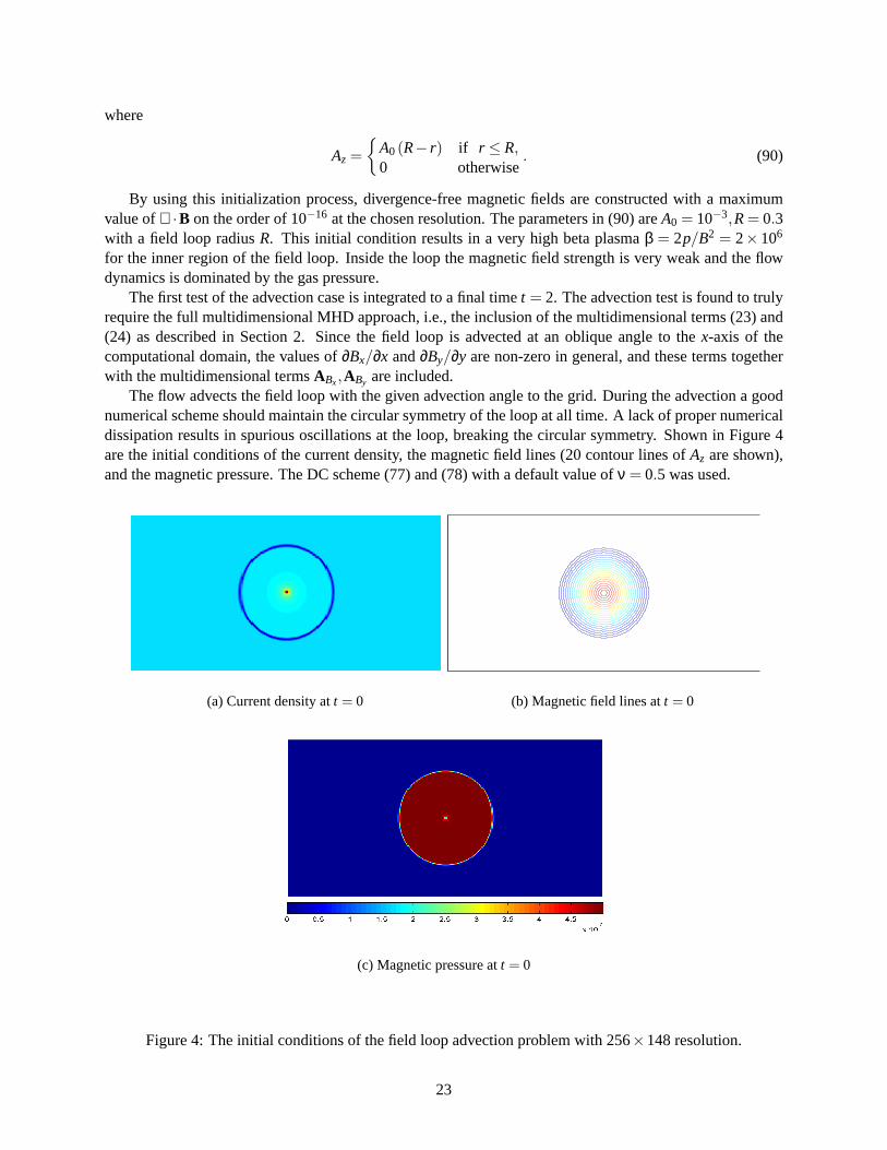
The flow advects the field loop with the given advection angle to the grid. During the advection a goodnumerical scheme should maintain the circular symmetry of the loop at all time. A lack of proper numericaldissipation results in spurious oscillations at the loop, breaking the circular symmetry. Shown in Figure 4are the initial conditions of the current density, the magnetic field lines (20 contour lines ofAz are shown),and the magnetic pressure. The DC scheme (77) and (78) with a default value ofν = 0.5 was used.
(a) Current density att = 0 (b) Magnetic field lines att = 0
(c) Magnetic pressure att = 0
Figure 4: The initial conditions of the field loop advection problem with 256×148 resolution.
23
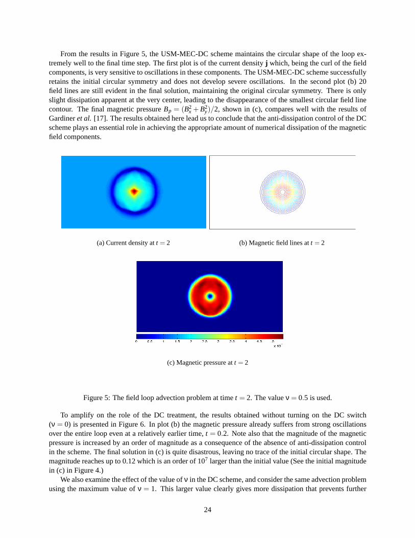
From the results in Figure 5, the USM-MEC-DC scheme maintains the circular shape of the loop ex-tremely well to the final time step. The first plot is of the current densityj which, being the curl of the fieldcomponents, is very sensitive to oscillations in these components. The USM-MEC-DC scheme successfullyretains the initial circular symmetry and does not develop severe oscillations. In the second plot (b) 20field lines are still evident in the final solution, maintaining the original circular symmetry. There is onlyslight dissipation apparent at the very center, leading to the disappearance of the smallest circular field linecontour. The final magnetic pressureBp = (B2
x + B2y)/2, shown in (c), compares well with the results of
Gardineret al. [17]. The results obtained here lead us to conclude that the anti-dissipation control of the DCscheme plays an essential role in achieving the appropriate amount of numerical dissipation of the magneticfield components.
(a) Current density att = 2 (b) Magnetic field lines att = 2
(c) Magnetic pressure att = 2
Figure 5: The field loop advection problem at timet = 2. The valueν = 0.5 is used.
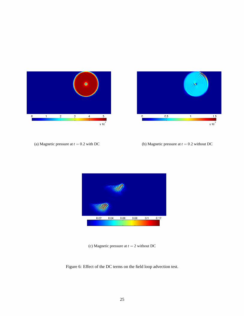
To amplify on the role of the DC treatment, the results obtained without turning on the DC switch(ν = 0) is presented in Figure 6. In plot (b) the magnetic pressure already suffers from strong oscillationsover the entire loop even at a relatively earlier time,t = 0.2. Note also that the magnitude of the magneticpressure is increased by an order of magnitude as a consequence of the absence of anti-dissipation controlin the scheme. The final solution in (c) is quite disastrous, leaving no trace of the initial circular shape. Themagnitude reaches up to 0.12 which is an order of 107 larger than the initial value (See the initial magnitudein (c) in Figure 4.)
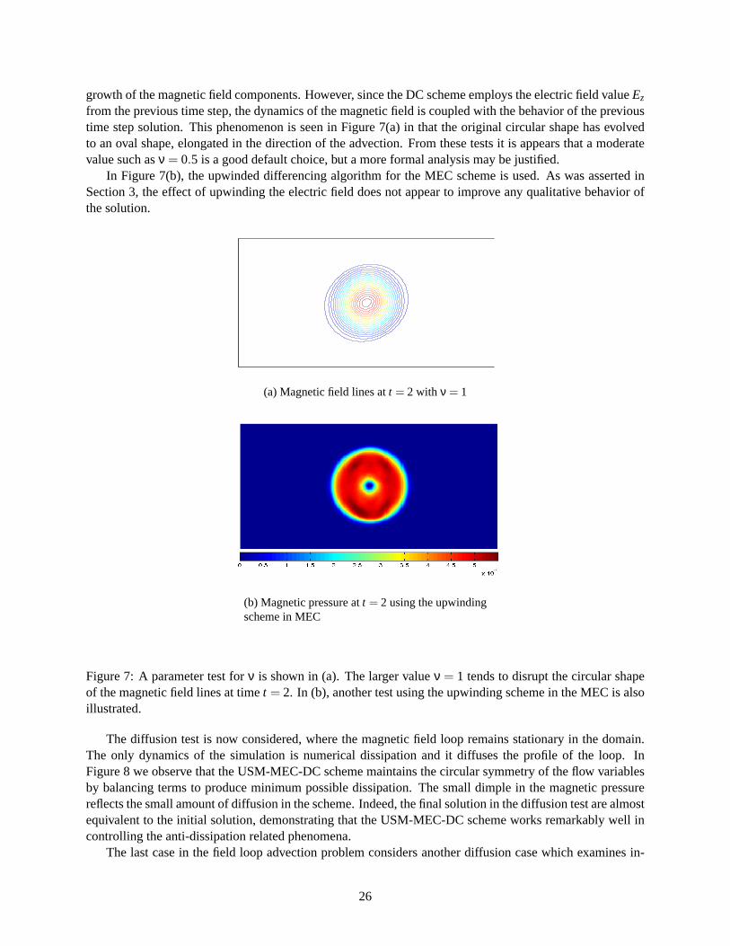
We also examine the effect of the value ofν in the DC scheme, and consider the same advection problemusing the maximum value ofν = 1. This larger value clearly gives more dissipation that prevents further
24
(a) Magnetic pressure att = 0.2 with DC (b) Magnetic pressure att = 0.2 without DC
(c) Magnetic pressure att = 2 without DC
Figure 6: Effect of the DC terms on the field loop advection test.
25
growth of the magnetic field components. However, since the DC scheme employs the electric field valueEz
from the previous time step, the dynamics of the magnetic field is coupled with the behavior of the previoustime step solution. This phenomenon is seen in Figure 7(a) in that the original circular shape has evolvedto an oval shape, elongated in the direction of the advection. From these tests it is appears that a moderatevalue such asν = 0.5 is a good default choice, but a more formal analysis may be justified.
In Figure 7(b), the upwinded differencing algorithm for the MEC scheme is used. As was asserted inSection 3, the effect of upwinding the electric field does not appear to improve any qualitative behavior ofthe solution.
(a) Magnetic field lines att = 2 with ν = 1
(b) Magnetic pressure att = 2 using the upwindingscheme in MEC
Figure 7: A parameter test forν is shown in (a). The larger valueν = 1 tends to disrupt the circular shapeof the magnetic field lines at timet = 2. In (b), another test using the upwinding scheme in the MEC is alsoillustrated.
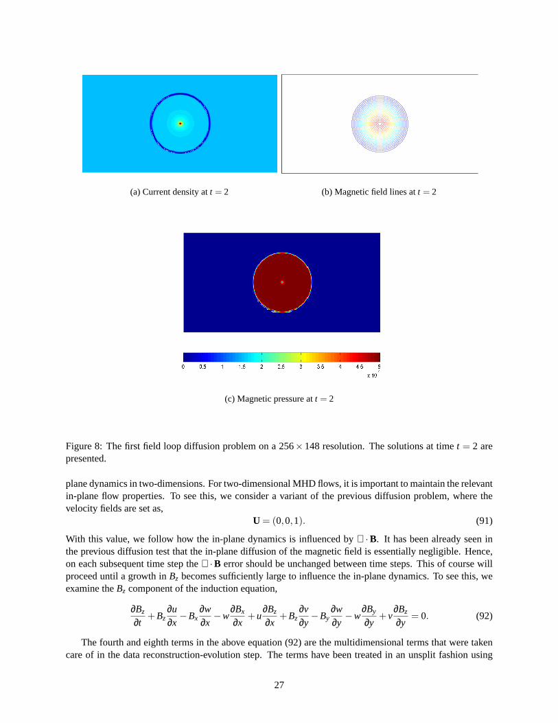
The diffusion test is now considered, where the magnetic field loop remains stationary in the domain.The only dynamics of the simulation is numerical dissipation and it diffuses the profile of the loop. InFigure 8 we observe that the USM-MEC-DC scheme maintains the circular symmetry of the flow variablesby balancing terms to produce minimum possible dissipation. The small dimple in the magnetic pressurereflects the small amount of diffusion in the scheme. Indeed, the final solution in the diffusion test are almostequivalent to the initial solution, demonstrating that the USM-MEC-DC scheme works remarkably well incontrolling the anti-dissipation related phenomena.
The last case in the field loop advection problem considers another diffusion case which examines in-
26
(a) Current density att = 2 (b) Magnetic field lines att = 2
(c) Magnetic pressure att = 2
Figure 8: The first field loop diffusion problem on a 256×148 resolution. The solutions at timet = 2 arepresented.
plane dynamics in two-dimensions. For two-dimensional MHD flows, it is important to maintain the relevantin-plane flow properties. To see this, we consider a variant of the previous diffusion problem, where thevelocity fields are set as,
U = (0,0,1). (91)
With this value, we follow how the in-plane dynamics is influenced by∇ ·B. It has been already seen inthe previous diffusion test that the in-plane diffusion of the magnetic field is essentially negligible. Hence,on each subsequent time step the∇ ·B error should be unchanged between time steps. This of course willproceed until a growth inBz becomes sufficiently large to influence the in-plane dynamics. To see this, weexamine theBz component of the induction equation,
∂Bz
∂t+Bz
∂u∂x−Bx
∂w∂x
−w∂Bx
∂x+u
∂Bz
∂x+Bz
∂v∂y−By
∂w∂y
−w∂By
∂y+v
∂Bz
∂y= 0. (92)
The fourth and eighth terms in the above equation (92) are the multidimensional terms that were takencare of in the data reconstruction-evolution step. The terms have been treated in an unsplit fashion using
27
the multidimensional characteristic method without applying any limiting (See equation (28)). The sumof these two terms isw∇ ·B = w(∆Bx,i/∆x+ ∆By, j/∆y), and hence if there is any secular growth in the∇ ·B = (∆Bx,i/∆x+∆By, j/∆y) error, it will change the in-plane geometry due to an unphysical growth ofBz
with a rate proportional tow∇ ·B∆t. For dimensionally split MHD schemes, this kind of unphysical growthis hard to avoid, since the terms∆Bx,i/∆x and∆By, j/∆y are not updated simultaneously.
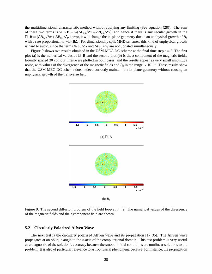
Figure 9 shows two results obtained in the USM-MEC-DC scheme at the final time stept = 2. The firstplot (a) is the numerical values of∇ ·B and the second plot (b) is thez component of the magnetic fields.Equally spaced 30 contour lines were plotted in both cases, and the results appear as very small amplitudenoise, with values of the divergence of the magnetic fields andBz in the range∼ 10−15. These results showthat the USM-MEC-DC scheme does indeed correctly maintain the in-plane geometry without causing anunphysical growth of the transverse field.
−1.5 −1 −0.5 0 0.5 1 1.5
x 10−15
(a) ∇ ·B
−1.5 −1 −0.5 0 0.5 1 1.5
x 10−15
(b) Bz
Figure 9: The second diffusion problem of the field loop att = 2. The numerical values of the divergenceof the magnetic fields and thez component field are shown.
5.2 Circularly Polarized Alfv en Wave
The next test is the circularly polarized Alfven wave and its propagation [17, 35]. The Alfven wavepropagates at an oblique angle to thex-axis of the computational domain. This test problem is very usefulas a diagnostic of the solution’s accuracy because the smooth initial conditions are nonlinear solutions to theproblem. It is also of particular relevance to astrophysical phenomena because, for instance, the propagation
28
of Alfv en waves in the solar wind is thought to be a possible source for the heating of the solar corona.Hence their accurate modeling is crucial. Further, departures from pure Alfvenic modes are a measure ofthe interaction of these waves with the solar wind [18,32].
The initial conditions we use are the same as the equivalent test problems described in [17]. A compu-tational domain with a doubly periodic box[0,1/cosθ]× [0,1/sinθ] is determined according to the propa-gation angleθ, and the value we adopt isθ = tan−1(2)≈ 63.44◦. In this configuration, flux terms involving∂Bx/∂x and∂By/∂y are non-zero throughout the domain and their contribution to the solution, especially themagnetic fields, are essential in this problem. For the convergence study we simulated both standing andtraveling Alfven waves.
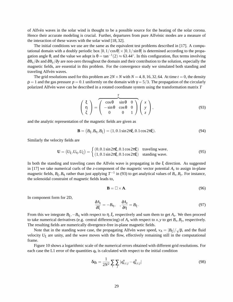
The grid resolutions used for this problem are 2N×N with N = 4,8,16,32,64. At timet = 0, the densityρ = 1 and the gas pressurep= 0.1 uniformly on the domain withγ = 5/3. The propagation of the circularlypolarized Alfven wave can be described in a rotated coordinate system using the transformation matrixT
ξηζ
=
T︷ ︸︸ ︷ cosθ sinθ 0−sinθ cosθ 0
0 0 1
xyz
, (93)
and the analytic representation of the magnetic fields are given as
B =(Bξ,Bη,Bζ
)= (1,0.1sin2πξ,0.1cos2πξ). (94)
Similarly the velocity fields are
U =(Uξ,Uη,Uζ
)={
(0,0.1sin2πξ,0.1cos2πξ) traveling wave,(1,0.1sin2πξ,0.1cos2πξ) standing wave.
(95)
In both the standing and traveling cases the Alfven wave is propagating in theξ direction. As suggestedin [17] we take numerical curls of thez-component of the magnetic vector potentialAz to assign in-planemagnetic fields,Bξ,Bη rather than just applyingT−1 in (93) to get analytical values ofBx,By. For instance,the solenoidal constraint of magnetic fields leads to,
B = ∇×A. (96)
In component form for 2D,∂Az
∂ξ=−Bη, ,
∂Az
∂η= Bξ. (97)
From this we integrateBξ,−Bη with respect toη,ξ, respectively and sum them to getAz. We then proceedto take numerical derivatives (e.g. central differencing) ofAz with respect tox,y to getBx,By, respectively.The resulting fields are numerically divergence-free in-plane magnetic fields.
Note that in the standing wave case, the propagating Alfven wave speed,vA = |Bξ|/√ρ, and the fluid
velocity Uξ are unity, and the wave moves with the flow, effectively remaining still in the computationalframe.
Figure 10 shows a logarithmic scale of the numerical errors obtained with different grid resolutions. Foreach case the L1 error of the quantitiesqk is calculated with respect to the initial condition
δqk =1
2N2 ∑i
∑j
|qnk,i, j −q0
k,i, j | (98)
29
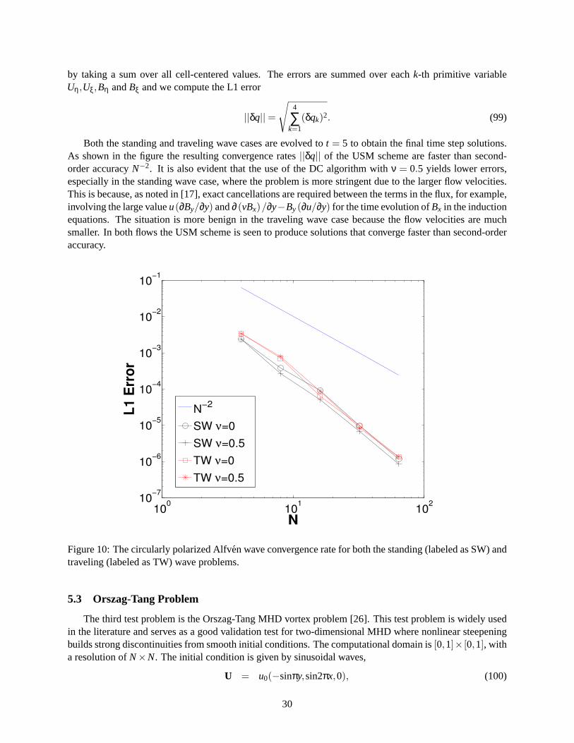
by taking a sum over all cell-centered values. The errors are summed over eachk-th primitive variableUη,Uξ,Bη andBξ and we compute the L1 error
||δq||=
√4
∑k=1
(δqk)2. (99)
Both the standing and traveling wave cases are evolved tot = 5 to obtain the final time step solutions.As shown in the figure the resulting convergence rates||δq|| of the USM scheme are faster than second-order accuracyN−2. It is also evident that the use of the DC algorithm withν = 0.5 yields lower errors,especially in the standing wave case, where the problem is more stringent due to the larger flow velocities.This is because, as noted in [17], exact cancellations are required between the terms in the flux, for example,involving the large valueu(∂By/∂y) and∂(vBx)/∂y−By(∂u/∂y) for the time evolution ofBx in the inductionequations. The situation is more benign in the traveling wave case because the flow velocities are muchsmaller. In both flows the USM scheme is seen to produce solutions that converge faster than second-orderaccuracy.
100
101
10210
−7
10−6
10−5
10−4
10−3
10−2
10−1
N
L1 E
rror
N−2
SW ν=0SW ν=0.5TW ν=0TW ν=0.5
Figure 10: The circularly polarized Alfven wave convergence rate for both the standing (labeled as SW) andtraveling (labeled as TW) wave problems.
5.3 Orszag-Tang Problem
The third test problem is the Orszag-Tang MHD vortex problem [26]. This test problem is widely usedin the literature and serves as a good validation test for two-dimensional MHD where nonlinear steepeningbuilds strong discontinuities from smooth initial conditions. The computational domain is[0,1]× [0,1], witha resolution ofN×N. The initial condition is given by sinusoidal waves,
U = u0(−sinπy,sin2πx,0), (100)
30
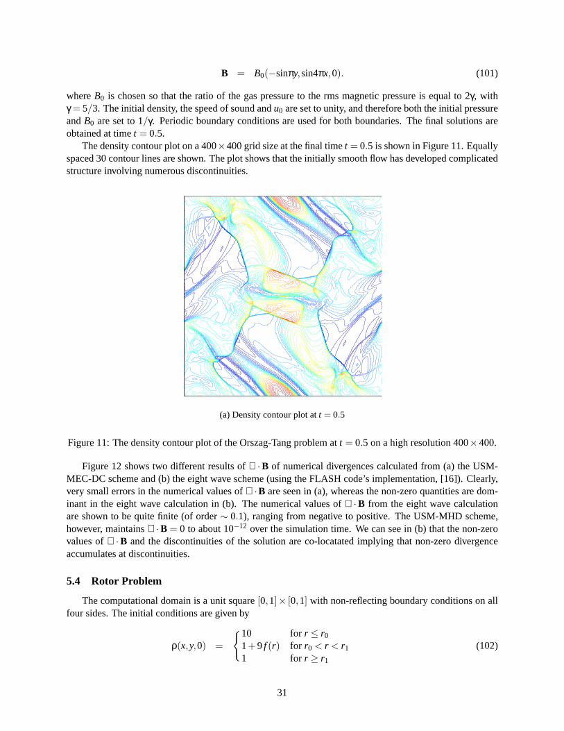
B = B0(−sinπy,sin4πx,0). (101)
whereB0 is chosen so that the ratio of the gas pressure to the rms magnetic pressure is equal to 2γ, withγ = 5/3. The initial density, the speed of sound andu0 are set to unity, and therefore both the initial pressureandB0 are set to 1/γ. Periodic boundary conditions are used for both boundaries. The final solutions areobtained at timet = 0.5.
The density contour plot on a 400×400 grid size at the final timet = 0.5 is shown in Figure 11. Equallyspaced 30 contour lines are shown. The plot shows that the initially smooth flow has developed complicatedstructure involving numerous discontinuities.
(a) Density contour plot att = 0.5
Figure 11: The density contour plot of the Orszag-Tang problem att = 0.5 on a high resolution 400×400.
Figure 12 shows two different results of∇ ·B of numerical divergences calculated from (a) the USM-MEC-DC scheme and (b) the eight wave scheme (using the FLASH code’s implementation, [16]). Clearly,very small errors in the numerical values of∇ ·B are seen in (a), whereas the non-zero quantities are dom-inant in the eight wave calculation in (b). The numerical values of∇ ·B from the eight wave calculationare shown to be quite finite (of order∼ 0.1), ranging from negative to positive. The USM-MHD scheme,however, maintains∇ ·B = 0 to about 10−12 over the simulation time. We can see in (b) that the non-zerovalues of∇ ·B and the discontinuities of the solution are co-locatated implying that non-zero divergenceaccumulates at discontinuities.
5.4 Rotor Problem
The computational domain is a unit square[0,1]× [0,1] with non-reflecting boundary conditions on allfour sides. The initial conditions are given by
ρ(x,y,0) =
{10 for r ≤ r0
1+9 f (r) for r0 < r < r1
1 for r ≥ r1
(102)
31
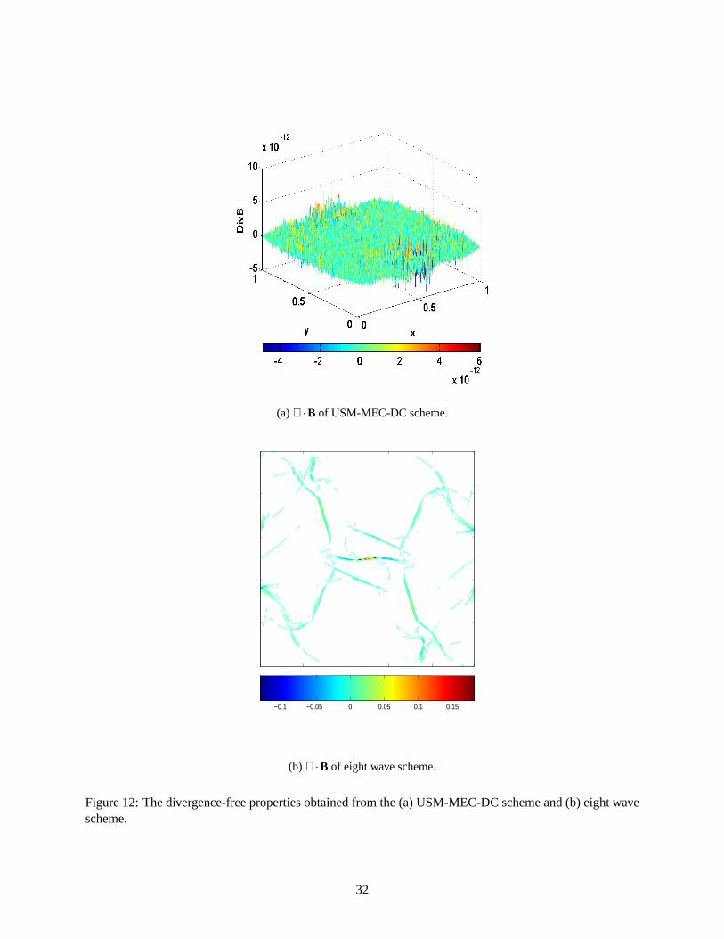
(a) ∇ ·B of USM-MEC-DC scheme.
−0.1 −0.05 0 0.05 0.1 0.15
(b) ∇ ·B of eight wave scheme.
Figure 12: The divergence-free properties obtained from the (a) USM-MEC-DC scheme and (b) eight wavescheme.
32
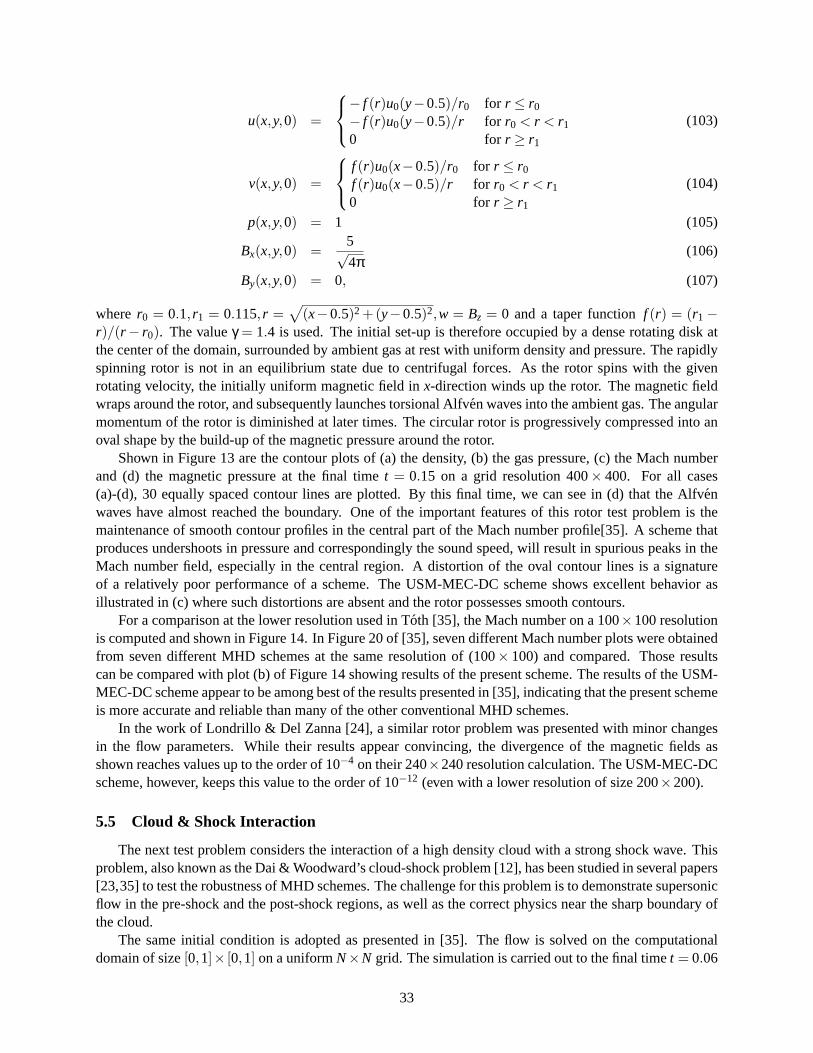
u(x,y,0) =
− f (r)u0(y−0.5)/r0 for r ≤ r0
− f (r)u0(y−0.5)/r for r0 < r < r1
0 for r ≥ r1
(103)
v(x,y,0) =
f (r)u0(x−0.5)/r0 for r ≤ r0
f (r)u0(x−0.5)/r for r0 < r < r1
0 for r ≥ r1
(104)
p(x,y,0) = 1 (105)
Bx(x,y,0) =5√4π
(106)
By(x,y,0) = 0, (107)
wherer0 = 0.1, r1 = 0.115, r =√
(x−0.5)2 +(y−0.5)2,w = Bz = 0 and a taper functionf (r) = (r1−r)/(r − r0). The valueγ = 1.4 is used. The initial set-up is therefore occupied by a dense rotating disk atthe center of the domain, surrounded by ambient gas at rest with uniform density and pressure. The rapidlyspinning rotor is not in an equilibrium state due to centrifugal forces. As the rotor spins with the givenrotating velocity, the initially uniform magnetic field inx-direction winds up the rotor. The magnetic fieldwraps around the rotor, and subsequently launches torsional Alfven waves into the ambient gas. The angularmomentum of the rotor is diminished at later times. The circular rotor is progressively compressed into anoval shape by the build-up of the magnetic pressure around the rotor.
Shown in Figure 13 are the contour plots of (a) the density, (b) the gas pressure, (c) the Mach numberand (d) the magnetic pressure at the final timet = 0.15 on a grid resolution 400× 400. For all cases(a)-(d), 30 equally spaced contour lines are plotted. By this final time, we can see in (d) that the Alfvenwaves have almost reached the boundary. One of the important features of this rotor test problem is themaintenance of smooth contour profiles in the central part of the Mach number profile[35]. A scheme thatproduces undershoots in pressure and correspondingly the sound speed, will result in spurious peaks in theMach number field, especially in the central region. A distortion of the oval contour lines is a signatureof a relatively poor performance of a scheme. The USM-MEC-DC scheme shows excellent behavior asillustrated in (c) where such distortions are absent and the rotor possesses smooth contours.
For a comparison at the lower resolution used in Toth [35], the Mach number on a 100×100 resolutionis computed and shown in Figure 14. In Figure 20 of [35], seven different Mach number plots were obtainedfrom seven different MHD schemes at the same resolution of (100× 100) and compared. Those resultscan be compared with plot (b) of Figure 14 showing results of the present scheme. The results of the USM-MEC-DC scheme appear to be among best of the results presented in [35], indicating that the present schemeis more accurate and reliable than many of the other conventional MHD schemes.
In the work of Londrillo & Del Zanna [24], a similar rotor problem was presented with minor changesin the flow parameters. While their results appear convincing, the divergence of the magnetic fields asshown reaches values up to the order of 10−4 on their 240×240 resolution calculation. The USM-MEC-DCscheme, however, keeps this value to the order of 10−12 (even with a lower resolution of size 200×200).
5.5 Cloud & Shock Interaction
The next test problem considers the interaction of a high density cloud with a strong shock wave. Thisproblem, also known as the Dai & Woodward’s cloud-shock problem [12], has been studied in several papers[23,35] to test the robustness of MHD schemes. The challenge for this problem is to demonstrate supersonicflow in the pre-shock and the post-shock regions, as well as the correct physics near the sharp boundary ofthe cloud.
The same initial condition is adopted as presented in [35]. The flow is solved on the computationaldomain of size[0,1]× [0,1] on a uniformN×N grid. The simulation is carried out to the final timet = 0.06
33
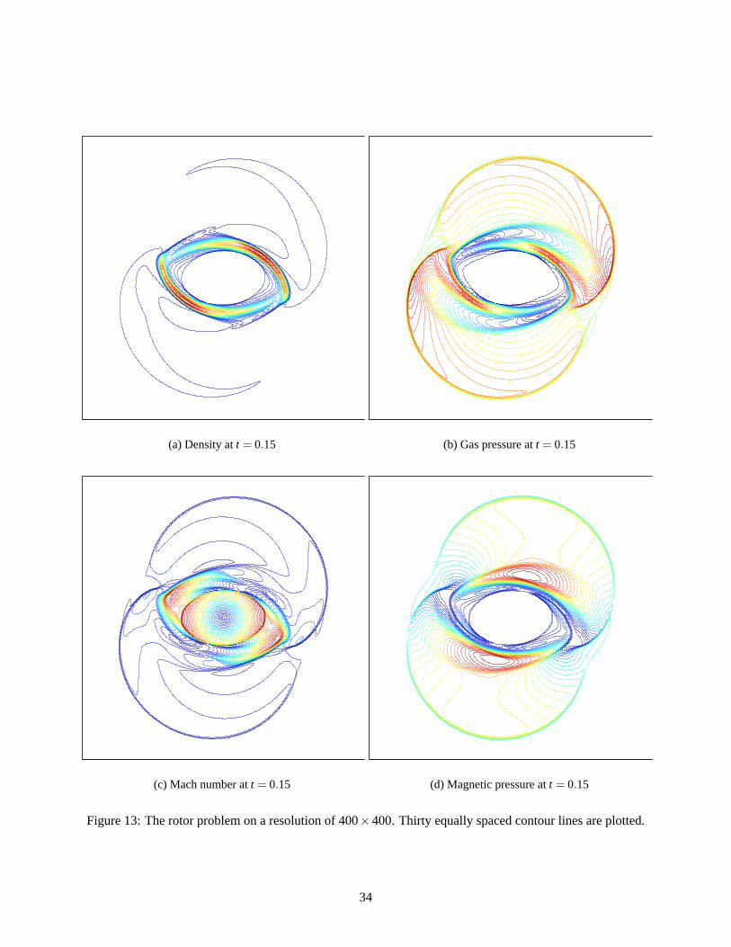
(a) Density att = 0.15 (b) Gas pressure att = 0.15
(c) Mach number att = 0.15 (d) Magnetic pressure att = 0.15
Figure 13: The rotor problem on a resolution of 400×400. Thirty equally spaced contour lines are plotted.
34
0 0.2 0.4 0.6 0.8 10
0.2
0.4
0.6
0.8
1
(a) Mach number att = 0.15
0.3 0.4 0.5 0.6 0.70.3
0.4
0.5
0.6
(b) A close up view at the center
Figure 14: The Mach number for the rotor problem on a resolution of 100× 100. Thirty equally spacedcontour lines are plotted. In (b) the circular shapes of the contour lines are well captured even with this lowresolution.
35
with N = 400. The initial discontinuity involves the left and right states along a linex = 0.6 parallel to they axis, with
(ρ,u,v,w,Bx,By,Bz, p) =
(3.86859,0,0,0,0,2.1826182,−2.1826182,167.345)
if x≤ 0.6,(1,−11.2536,0,0,0,0.56418958,0.56418958,1)
if x > 0.6.
(108)
The high density cloud is located on the right side of the domain, for which its circular shape is definedby (x−0.8)2 +(y−0.5)2 = 0.152. Uniform densityρ = 10 and the pressurep = 1 are fixed in the innerregion, andγ = 5/3. The velocity and the magnetic fields are the same as the surrounding right state plasmavalues. Supersonic inflow boundary conditions are imposed along the right-most boundary atx = 1 andoutflow boundary conditions are used for all other boundaries.
As shown in the density plots in Figure 15, the temporal evolution involves the disruption of the highdensity cloud by the shock initially located atx = 0.6. The light areas indicate the strongly shocked regionsand compare well with the results in [23, 35]. It was found by Toth that a simple dimensionally split MHDalgorithm can easily fail due to unphysical states (e.g., negative pressure or density) produced during thestrong interaction of the shock with the cloud even when the rather diffusive MINMOD limiter was used. Inthe USM-MEC-DC scheme, the final time step is reached successfully without such problems.
5.6 MHD Blast Wave
The last test case presented is the MHD spherical blast wave problem of Zacharyet al. [37]. Thisproblem leads to the formation and propagation of strong MHD discontinuities, relevant to astrophysicalphenomena where the magnetic field energy has strong dynamical effects. With a numerical scheme thatfails to preserve the divergence-free constraint, unphysical states can be obtained involving negative gaspressure because the background magnetic pressure increases the strength of magnetic monopoles.
This problem was computed in two different flow regimes by taking intermediate and strong magneticfield strengths. The computational domain is a square[−0.5,0.5]× [−0.5,0.5] with a grid of resolution200×200. The explosion is driven by an over-pressurized circular region at the center of the domain witha radiusr = 0.1. The initial density is unity everywhere. The pressure of the ambient gas is 0.1, while thepressure of the inner region is 1000. Two different regimes of a uniform magnetic field in thex-directionare studied, withBx = 50/
√4π and 100/
√4π. These intial conditions result in very low-β ambient plasma
states,β = 1×10⁻³ and 2.513×10⁻⁴ respectively. Through these low-β ambient states, the explosion emitsalmost spherical fast magneto-sonic shocks that propagate with the fastest wave speed. The flow hasγ = 1.4.
The intermediate magnetic field strength case withBx = 50/√
4π is illustrated in Figure 16. We seean anisotropic explosion behavior because of the existence of the non-zero magnetic field strength inx-direction. With this value of theBx field, the shock waves still somewhat preserve the spherically symmetricshapes, although the development of the elongated wave structures in the direction parallel to theBx fieldare evident.
For a stronger magnetic field strengthBx = 100/√
4π, shown in Figure 17, the explosion now becomeshighly anisotropic. In Figure 17(b), the displacement of gas in the transversaly-direction is increasinglyinhibited and hydrodynamical shocks propagate in both positive and negativex-directions parallel toBx. Itis also evident in (d) that several weak magneto-sonic waves are radiated transverse tox-direction. Thisprocess continues until total pressure equilibrium is reached in the central region.
Balsara [4] found that the strong wave propagation oblique to the mesh can cause unphysical negativityin the pressure. Such effects are manifested as distortions of contours especially near the outer bound-ary, where a large and unphysical drop in pressure takes place immediately ahead of the shock. No suchexcrescence is evident in our calculation.
36
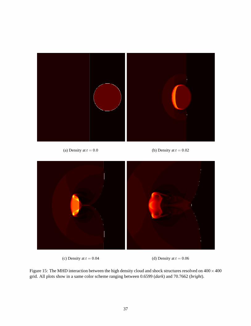
(a) Density att = 0.0 (b) Density att = 0.02
(c) Density att = 0.04 (d) Density att = 0.06
Figure 15: The MHD interaction between the high density cloud and shock structures resolved on 400×400grid. All plots show in a same color scheme ranging between 0.6599 (dark) and 70.7662 (bright).
37
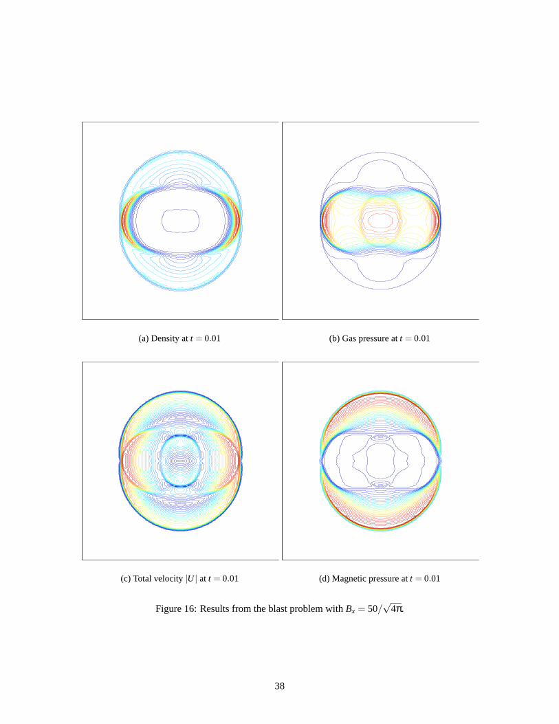
(a) Density att = 0.01 (b) Gas pressure att = 0.01
(c) Total velocity|U | at t = 0.01 (d) Magnetic pressure att = 0.01
Figure 16: Results from the blast problem withBx = 50/√
4π.
38
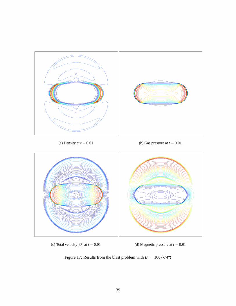
(a) Density att = 0.01 (b) Gas pressure att = 0.01
(c) Total velocity|U | at t = 0.01 (d) Magnetic pressure att = 0.01
Figure 17: Results from the blast problem withBx = 100/√
4π.
39
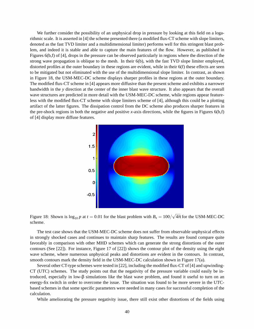
We further consider the possibility of an unphysical drop in pressure by looking at this field on a loga-rithmic scale. It is asserted in [4] the scheme presented there (a modified flux-CT scheme with slope limiters,denoted as the fast TVD limiter and a multidimensional limiter) performs well for this stringent blast prob-lem, and indeed it is stable and able to capture the main features of the flow. However, as published inFigures 6(b,f) of [4], drops in the pressure can be observed particularly in regions where the direction of thestrong wave propagation is oblique to the mesh. In their 6(b), with the fast TVD slope limiter employed,distorted profiles at the outer boundary in these regions are evident, while in their 6(f) these effects are seento be mitigated but not eliminated with the use of the multidimensional slope limiter. In contrast, as shownin Figure 18, the USM-MEC-DC scheme displays sharper profiles in these regions at the outer boundary.The modified flux-CT scheme in [4] appears more diffusive than the present scheme and exhibits a narrowerbandwidth in they direction at the center of the inner blast wave structure. It also appears that the overallwave structures are predicted in more detail with the USM-MEC-DC scheme, while regions appear feature-less with the modified flux-CT scheme with slope limiters scheme of [4], although this could be a plottingartifact of the latter figures. The dissipation control from the DC scheme also produces sharper features inthe pre-shock regions in both the negative and positivex-axis directions, while the figures in Figures 6(b,f)of [4] display more diffuse features.
Figure 18: Shown is log10 p at t = 0.01 for the blast problem withBx = 100/√
4π for the USM-MEC-DCscheme.
The test case shows that the USM-MEC-DC scheme does not suffer from observable unphysical effectsin strongly shocked cases and continues to maintain sharp features. The results are found compare quitefavorably in comparison with other MHD schemes which can generate the strong distortions of the outercontours (See [22]). For instance, Figure 17 of [22]) shows the contour plot of the density using the eightwave scheme, where numerous unphysical peaks and distortions are evident in the contours. In contrast,smooth contours mark the density field in the USM-MEC-DC calculation shown in Figure 17(a).
Several other CT-type schemes were tested in [22], including the modified flux-CT of [4] and upwinding-CT (UTC) schemes. The study points out that the negativity of the pressure variable could easily be in-troduced, especially in low-β simulations like the blast wave problem, and found it useful to turn on anenergy-fix switch in order to overcome the issue. The situation was found to be more severe in the UTC-based schemes in that some specific parameters were needed in many cases for successful completion of thecalculation.
While ameliorating the pressure negativity issue, there still exist other distortions of the fields using
40
these schemes as indicated in Figure 19 of [22]). It can also be seen in plots of their so-labeled BS2 and BS3that, as mentioned earlier, there appears to be no qualitative difference between the results when adoptingthe comparatively newer reconstruction scheme of [4], equations (86) and (87).
6 Conclusion
The USM-MEC-DC scheme has been introduced, developed and studied in this paper. The methoduses characteristic analysis to account for the contribution of both normal and transversal MHD fluxes. Amodified electric field construction (MEC) scheme and a new, very efficient, dissipation control algorithm(DC) has been presented. The results of several test problems presented give considerable confidence in thescheme for use as a robust and reliable second-order MHD algorithm.
The second-order accurate, multidimensional, unsplit high-order Godunov MHD algorithm has beensuccessfully developed on a staggered grid, with the capability of maintaining divergence-free magneticfields numerically. The method preserves the constraint numerically extremely well without evidence ofnumerical instability or accumulation of unphysical errors. As validation, the suite of test problems pre-sented in this study include several stringent setups that stress various features of MHD algorithms. Theyconsist of the evolution of a very weak magnetic field loop, a convergence study of circularly polarizedAlfv en waves, the widely used benchmark Orszag-Tang vortex problem, the spinning rotor problem, mag-netic cloud-shock interaction, and the MHD blast wave problem. The scheme has been thoroughly testedand has been shown to perform very well, providing confidence in correctly simulating a wide range ofMHD physical phenomena.
The scheme handles multidimensional MHD terms consistently using the characteristic method. Suchmultidimensional treatment has been ignored in many of the operator splitting based MHD schemes. Theapproach involves physical considerations that multidimensional MHD schemes should manifest. In partic-ular, such multidimensional considerations eliminate unphysical secular growth that would cause deviationsfrom the in-plane dynamical evolution. To ascertain this, a two-dimensional MHD problem of field loopdiffusion was computed. Spurious numerical errors proportional to∇ ·B would affect the growth ofBz, andultimately alter the in-plane dynamics of the problem. These were found to be absent. The presented datareconstruction-evolution method resolves the issue by using the multidimensional characteristic method ina straightforward way.
A new procedure has been developed to construct the electric field in the MEC scheme, which appearsto significantly improve the accuracy of similar schemes (e.g., the flux-CT scheme of Reference [2]). TheMEC scheme takes a more directional consideration of the high-order Godunov fluxes obtained from theduality relationship in the flux-CT scheme.
Remarkably good results are found with the introduction and development of the DC scheme for theinduction equation, in that a significant improvement in the solution of magnetic fields is found, which isparticularly observable in the field loop tests. We find that for our scheme, without utilizing the DC schemefor the simulation, the circular symmetry of the field loop is destroyed. A balancing of the numericaldissipation in MHD schemes is found to be important not only for the accuracy of solutions, but evenfor stability. The DC scheme provides insight into suppressing undesirable anti-dissipative effects thatpotentially exist in the solving the induction equation.
This paper has detailed the core algorithmic features of the USM-MEC-DC scheme, laying down theimportant multidimensional aspects, and subjecting it to a series of tests. In subsequent publications we willpresent extensions of this scheme that support parallel adaptive mesh refinement (early parallel results werereported in [21]) and implementation in fully three dimensions.
The scheme has been implemented and is currently available in the University of Chicago ASC FLASHCenter’s FLASH 3 release [16].
41
7 Acknowledgments
This work has been supported in part by National Science Foundation ITR grant DMS-0219282. TheFLASH code has been developed by the DOE-supported ASC/Alliance Center for Astrophysical Thermonu-clear Flashes at the University of Chicago. This work is supported by the U.S. Department of Energy underGrant No. B523820 to the Center for Astrophysical Thermonuclear Flashes at the University of Chicago.The first author gratefully acknowledge the FLASH code group for help and for supporting the current work.The authors would like to thank Dr. James Stone at Princeton University and Dr. Timur Linde, previouslyat the FLASH center and now in industry, for useful discussions and comments on an early work of thispaper. We also acknowledge useful discussions with Dr. Robert Fisher at the FLASH center, University ofChicago. The authors especially thank Dr. Kevin Olson at the Drexel University for helpful support duringthe course of this work.
References
1 Balsara, D. S., Total Variation Diminishing Scheme for Adiabatic and Isothermal Magnetohydrodynam-ics, Astrophys. J. Suppl., 116:133–153, 1998.
2 Balsara, D. S., Spicer, D. S., A Staggered Mesh Algorithm Using High Order Godunov Fluxes to EnsureSolenoidal Magnetic Fields in Magnetohydrodynamics Simulation,J. Comput. Phys., 149:270–292,1999.
3 Balsara, D. S., Divergence-Free Adaptive Mesh Refinement for Magnetohydrodynamics,J. Comput.Phys., 174:614–648, 2001.
4 Balsara, D. S., Second-Order-Accurate Schemes For Magnetohydrodynamics With Divergence-FreeReconstruction,Astrophys. J. Suppl., 151:149–184, 2004.
5 Balsara, D. S., Kim, D., An Intercomparison Between Divergence-Cleaning and Staggered Mesh For-mulations for Numerical Magnetohydrodynamics,Astrophys. J., 602:1079-1090, 2004 February 202004.
6 Brackbill, J. U., Barnes, D. C., The Effect of Nonzero∇ ·B. on the Numerical Solution of the Magneto-hydrodynamic Equations,J. Comput. Phys., 87:171–200, 1990.
7 Brecht, S. H., Lyon, J. G., Fedder, J. A., Hain, K.,Geophys. Res. Lett., 8:397, 1981.
8 Brio, M., Wu, C. C., An Upwind Differencing Scheme for the Equations of Ideal Magnetohydrodynam-ics, J. Comput. Phys., 75:400–422, 1988.
9 Colella, P., Multidimensional Upwind Methods for Hyperbolic Conservation Laws,J. Comput. Phys.,87:171–200, 1990.
10 Crockett, R. K., Colella, P., Fisher, R. T., Klein, R. I., McKee, C. F., An Unsplit, Cell-Centered GodunovMethod for Ideal MHD,J. Comput. Phys., 203:422–448, 2005.
11 Dai, W., Woodward, P., An Approximate Riemann Solver for Ideal Magnetohydrodynamics,J. Comput.Phys., 111:354–372, 1994.
12 Dai, W., Woodward, P., A Simple Finite Difference Scheme for Multidimensional Magnetohydrody-namics,J. Comput. Phys., 142:331–369, 1998.
42
13 Dedner, A., Kemm, F., Kroner, D., Munz, C. D., Schnitzer, T., Wesenberg, M., Hyperbolic DivergenceCleaning for the MHD Equations,J. Comput. Phys., 175:645–673, 2002.
14 DeVore, C. R., Flux Corrected Transport Techniques for Multidimensional Compressible Magnetohy-drodynamics,J. Comput. Phys., 92:142, 1991.
15 Evans, C. R., Hawley, J. F., Simulation of Magnetohydrodynamic Flows: A Constrained TransportMethod,Astrophys. J., 332:659–677, 1988.
16 FLASH, <http://flash.uchicago.edu>, 2007.
17 Gardiner, T., Stone, J., An Unsplit Godunov Method for Ideal MHD via Constrained Transport,J.Comput. Phys., 205:509–539, 2005.
18 Goldstein, M. L., Roberts, D. A., Deane, A. E., Ghosh, S., Numerical Simulation of Alfvenic Turbulencein the Solar Wind,J. Geophys. Res., 104, A7:14437–14451, 1999.
19 Goldstein, M. L., Roberts, D. A., Burlaga, L. F., Sirigar, E., Deane,A. E., North-south flows observedin the outer heliosphere at solar minimum: Vortex streets or corotating interaction regions?,J. Geophys.Res., 106, A8:15973–15984, 2001.
20 Janhunen, P., A Positive Conservative Method for Magnetohydrodynamics Based on HLL and RoeMethods,J. Comput. Phys., 160:649, 2000.
21 Lee, D., Deane, A., A Parallel Unsplit Staggered Mesh Algorithm for Magnetohydrodynamics, ParallelCFD, Egmond En Zee, Netherlands, 2005.
22 Li, S., Note on Upwinding Constrained Transport Method for Ideal Magnetohydrodynamics,LosAlamos Report, LA-UR-03-8925, 2003.
23 Li, S., Li, H., A Modern Code for Magneto-hydrodynamics or Hydrodynamics Equations,Los AlamosReport, LA-UR-03-8925, 2003.
24 Londrillo, P., Del Zanna, L., High Order Upwind Schemes For Multidimensional Magnetohydrodynam-ics, Astrophys. J., 530:508–524, 2000.
25 Londrillo, P., Del Zanna, L., On the Divergence-Free Condition in Godunov-Type Schemes for IdealMagnetohydrodynamics: The Upwind Constrained Transport Method,J. Comput. Phys., 195:14–48,2004.
26 Orszag, A., Tang, C. M., Small-scale Structure of Two-Dimensional Magnetohydrodynamics Turbu-lence,J. Fluid Mech., 90:129–143, 1979.
27 Pen, U., Arras, P., Wong, S., A Free, Fast, Simple and Efficient TVD MHD Code,Astrophys. J. Suppl.,149:447–455, 2003.
28 Powell, K. G., A Riemann Solver for Ideal MHD: That works in More Than One Dimension, ICASEReport, 94–24, Langely, VA, 1994.
29 Powell, K. G., Roe, P. L., Linde, T. J., Gombosi, T. I., De Zeeuw, D. L., A Solution-Adaptive UpwindScheme for Ideal Magnetohydrodynamics,J. Comput. Phys., 154:284–309, 1999.
30 Ryu, D, Jones, T. W., Numerical Magnetohydrodynamics in Astrophysics: Algorithm and Tests forOne-dimensional Flow,Astrophys. J., 442:228–258, 1995.
43
31 Ryu, D, Miniati, F., Jones, T. W., Frank, A., A Divergence-Free Upwind Code For MultidimensionalMagnetohydrodynamic Flow,Astrophys. J., 509:244–255, 1999.
32 Ruderman, M. S., Goldstein, M. L., Roberts, D. A., Deane, A. E., Ofman, L., Alfven wave phasemixing driven by velocity shear in two-dimensional open magnetic configurations,J. Geophys. Res.,104, A8:17057–17068, 1999.
33 Stone, J., The Athena Test Suite,<http://www.astro.princeton.edu/∼jstone>
34 Toro, E. F., Riemann Solvers and Numerical Methods for Fluid Dynamics, A Practical Introduction,Springer, 1997.
35 Toth, G., The∇ ·B = 0 Constraint in Shock-Capturing Magnetohydrodynamics Codes,J. Comput.Phys., 161:605–656, 2000.
36 Yee, K. S. Numerical Solution of Initial Boundary Value Problems Involving Maxwell’s Equations inIsotropic MediaIEEE Trans. Antenna Propagation, AP-14:302–307
37 Zachary, A., Malagoli, A., Colella, P., A Higher-Order Godunov Method for Multidimensional IdealMagnetohydrodynamics,J. Comput. Phys., 2:263–284, 1994.
44