Prerequisites - learner.org · Additional coverage of ANOVA can be found in The Basic Practice of Statistics, Chapter 25, ... 0.35 0.40 0.45 0.50 0.55 0.60 0.65 0.70 4 3 2 1 0

Unit 31: One-Way ANOVA | Faculty Guide | Page 1

PrerequisitesStudents should be familiar with comparative boxplots covered in Unit 5, Boxplots. In addition, students need to have a background on significance tests. At a minimum, they should be familiar with the material covered in Unit 25, Tests of Significance, and Unit 27, Comparing Two Means. An understanding of experiments contained in Unit 15, Designing Experiments, would also be useful.

Additional Topic CoverageAdditional coverage of ANOVA can be found in The Basic Practice of Statistics, Chapter 25, One-Way Analysis of Variance: Comparing Several Means.

Activity DescriptionIn this activity, students conduct three experiments to see if changing control settings in a manufacturing process affects the mean thickness of a product, polished wafers used to make microchips. Students use Wafer Thickness from the Interactive Tools to collect data. In each experiment, two of the three Control settings are fixed at level 2, the middle setting, and the third is varied from level 1, to 2, to 3. Samples of size 10 are collected using Real Time mode so that students can watch the data being collected. The data can be copied by hand and then entered into software or graphing calculators for analysis. Students can also save the data in CVS format and then transfer their individual data sets into statistical or spreadsheet software for analysis.

Because the applet generates random data, each student (or group of students) will be working with different data. However, the results should be similar:

• For Control 1, the mean thickness differs among control levels.

• For Control 2, there is insufficient evidence to conclude that mean thickness differs among the control levels.

Unit 31: One-Way ANOVA


• For Control 3, the underlying assumption of equal standard deviations is not satisfied. Hence, the data are not analyzed by ANOVA.

This would be a good opportunity to show students that repeating the same experiment results in a different value for the F-statistic. Generally, the conclusions will be the same. However, it is possible that some students’ conclusions will differ from the majority due to sampling variability.

MaterialsStudents need access to the Wafer Thickness tool.


The Video Solutions

Take out a piece of paper and be ready to write down answers to these questions as you watch the video.

1. The average of all of the guesses will probably be more accurate than most of the individual guesses.

2. The weights of the clipboards differed. One weighed around one pound, another around two pounds, and a third around three pounds.

3. The population mean estimates are the same regardless of which clipboard is being held: H0 : µ1 = µ2 = µ2 .

4. ANOVA results in an F-statistic.

5. No. The p-value was above 0.05. Hence, he could not reject the null hypothesis based on the data.

6. Yes. The mean guess from the crowd was around $100 off from the actual amount of money in the jar. But that was closer to the actual amount of money in the jar than the guesses of three-quarters of the students.


Unit Activity: Controlling Wafer Thickness Solutions

1. a. - c. Sample answers based on sample data below.

d. Sample answer: It appears that mean thickness increases as the level of Control 1 is increased. Below are the sample means. The difference among the sample means appears large compared to the variability within each sample. Based on the histograms, although there is overlap between data values collected when Control 1 = 1 and Control 1 = 3, there is a considerable amount of shift.

Control 1 = 1 Control 1 = 2 Control 1 = 30.448 0.483 0.540.427 0.617 0.5960.527 0.508 0.5770.508 0.515 0.6090.461 0.405 0.6320.507 0.554 0.6310.388 0.531 0.660.409 0.587 0.5030.404 0.568 0.5830.512 0.555 0.583

Activity 1(a -‐ c)0.700.650.600.550.500.450.400.35

4

3

2

1

0

0.700.650.600.550.500.450.400.35

4

3

2

1

0

Control 1 = 1

Freq

uenc

y

Control 1 = 2

Control 1 = 3


e. Output from Minitab:

The null hypothesis is that the mean thickness of polished wafers was the same regardless of Control 1’s setting. The value of F and its p-value are highlighted in the ANOVA table above. The conclusion is that there are differences among the population mean thickness for wafers produced under the levels 1, 2, and 3 of Control 1.

2. a. Sample answer based on sample data in table below.

b. Sample answer: Yes. The standard deviations for the three samples are 0.050, 0.052, and 0.050, which are very close.

c. Output from Minitab is shown below. Values for F and p are highlighted.

3. a. Sample answer based on sample data in table below.

Control Level Sample Mean Standard Deviation1 0.459 0.05152 0.532 0.05963 0.591 0.0460

Activty 1(d)

Faculty Guide, Unit 31, OneWay ANOVA Page 4


Source DF SS MS F P Factor 2 0.08785 0.04392 15.85 0.000 Error 27 0.07487 0.00277 Total 29 0.16271 The null hypothesis is that the mean thickness of polished wafers was the same regardless of Control 1’s setting. The value of and its value are highlighted in the ANOVA table above. The conclusion is that there are differences among the population mean thickness for wafers produced under the levels 1, 2, and 3 of Control 1. 2. a. Sample answer based on sample data in table below.

Control 2 = 1 Control 2 = 2 Control 2 = 3 0.534 0.521 0.472 0.522 0.45 0.574 0.506 0.521 0.496 0.454 0.495 0.623 0.579 0.514 0.62 0.496 0.481 0.539 0.485 0.414 0.52 0.618 0.497 0.514 0.465 0.553 0.539 0.522 0.603 0.574


c. Output from Minitab is shown below. Values for and are highlighted.

Source DF SS MS F P Factor 2 0.00932 0.00466 1.80 0.185 Error 27 0.06991 0.00259 Total 29 0.07923 3. a. Sample answer based on sample data in table below.

Control 3 = 1 Control 3 = 2 Control 3 = 3 0.425 0.494 0.456 0.528 0.525 0.473 0.609 0.573 0.505 0.616 0.493 0.473



Source DF SS MS F P Factor 2 0.08785 0.04392 15.85 0.000 Error 27 0.07487 0.00277 Total 29 0.16271 The null hypothesis is that the mean thickness of polished wafers was the same regardless of Control 1’s setting. The value of and its value are highlighted in the ANOVA table above. The conclusion is that there are differences among the population mean thickness for wafers produced under the levels 1, 2, and 3 of Control 1. 2. a. Sample answer based on sample data in table below.

Control 2 = 1 Control 2 = 2 Control 2 = 3 0.534 0.521 0.472 0.522 0.45 0.574 0.506 0.521 0.496 0.454 0.495 0.623 0.579 0.514 0.62 0.496 0.481 0.539 0.485 0.414 0.52 0.618 0.497 0.514 0.465 0.553 0.539 0.522 0.603 0.574


c. Output from Minitab is shown below. Values for and are highlighted.

Source DF SS MS F P Factor 2 0.00932 0.00466 1.80 0.185 Error 27 0.06991 0.00259 Total 29 0.07923 3. a. Sample answer based on sample data in table below.

Control 3 = 1 Control 3 = 2 Control 3 = 3 0.425 0.494 0.456 0.528 0.525 0.473 0.609 0.573 0.505 0.616 0.493 0.473


Activity 2a


b. Sample answer: No. The standard deviations for the three samples are 0.098, 0.048, and 0.021. The ratio 0.098/0.021 is around 4.7, considerably more than twice as large.

c. The answer to (b) was No – so, we have skipped this part.


Activity 3a


Exercise Solutions

1. a.

b. Sample answer: It looks as if the students who studied with white noise did slightly better than students who studied with no sound. However, it’s difficult to tell if that difference is significant. It could be due to chance variation.

c. Hypotheses:

H0 : µWhite Noise = µMusic = µNo Noise

: There is some difference in the population means.aH

variation among sample meansvariation among individuals in same sample

MSGFMSE

= =

To calculate the MSG, we first have to calculate the grand mean, the mean of all the observations: x =5.556. Next, we need to calculate the deviations of the group means from the grand mean:

6.778 – 5.556 = 1.222; 5.444 – 5.556 = -0.112; 4.444 – 5.556 = -1.112

2 2 29(1.222) 9( 0.112) 9( 1.112) 24.6813 12.343 1 2

MSG + − + −= = ≈−

Group Mean Standard Deviation

White Noise 6.778 2.108

Music 5.444 1.59No Sound 4.444 1.59

Exercise 1a

108642

White noise

Music

No sound

Test

Soun

d


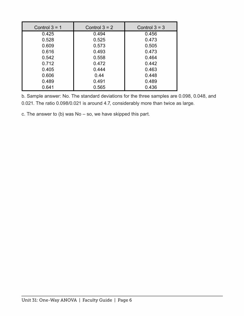
To calculate the MSE, we need the standard deviations for the test scores in each of the groups.

2 2 2(9 1)(2.108) (9 1)(1.590) (9 1)(1.509) 73.9989 3.0827 3 24

MSE − + − + −= = ≈−

F = 12.34/3.08 ≈ 4.01

F has numerator degrees of freedom 2 and denominator degrees of freedom 24.

d. Using statistical software, we can calculate the p-value from an F distribution as shown below. This gives a p-value of 0.03168. Conclusion: Reject the null hypothesis; conclude that the mean test scores differ depending on the surrounding sound during the study time.

Compare this value to the output from ANOVA (p-value is highlighted):

2. a. Standard deviations: Beef – 31.97; Poultry – 27.16; Veggie – 22.24.

The largest standard deviation is only about 1.4 times the smallest standard deviation. So, it’s reasonable to run an ANOVA on these data.

b. Below is the ANOVA table. The value of the F-statistic and p-value are highlighted. The numerator and denominator degrees of freedom for F are 2 and 19 + 19 + 18 = 56, respectively. Given the p-value is essentially 0, the conclusion is that there is some difference among the population mean calories of the Beef, Poultry, and Veggie hot dogs.

1.0

0.8

0.6

0.4

0.2

0.0

X

Dens

ity

400.03168

Distribution PlotF, df1=2, df2=24


has numerator degrees of freedom 2 and denominator degrees of freedom 24. d. Using statistical software, we can calculate the value from an distribution as shown below. This gives a value of 0.03168. Conclusion: Reject the null hypothesis; conclude that the mean test scores differ depending on the surrounding sound during the study time.

Compare this value to the output from ANOVA (value is highlighted): Source DF SS MS F P Sound 2 24.67 12.33 4.00 0.032 Error 24 74.00 3.08 Total 26 98.67 2. a. Standard deviations: Beef – 31.97; Poultry – 27.16; Veggie – 22.24. The largest standard deviation is only about 1.4 times the smallest standard deviation. So, it’s reasonable to run an ANOVA on these data. b. Below is the ANOVA table. The value of the statistic and value are highlighted. The numerator and denominator degrees of freedom for are 2 and 19 + 19 + 18 = 56, respectively. Given the value is essentially 0, the conclusion is that there is some difference among the population mean calories of the Beef, Poultry, and Veggie hot dogs.

Source DF SS MS F P Factor 2 101620 50810 67.20 0.000 Error 56 42344 756 Total 58 143964 c. From ANOVA, we know there is a significant difference in the mean calorie content among the three types of hot dogs. The boxplot shows that while all three types of hotdogs have some overlap in terms of calorie content, it appears that, on average, beef hotdogs have the highest mean calories, then poultry, and last veggie. There is more overlap in the boxplots between the Poultry and Veggie hotdogs – so, it is not as clear


c. From ANOVA, we know there is a significant difference in the mean calorie content among the three types of hot dogs. The boxplot shows that while all three types of hotdogs have some overlap in terms of calorie content, it appears that, on average, beef hotdogs have the highest mean calories, then poultry, and last veggie. There is more overlap in the boxplots between the Poultry and Veggie hotdogs – so, it is not as clear that their mean calorie contents differ significantly. (Keep in mind that ANOVA only says that at least one of the population means differs from the others. It doesn’t guarantee that all three population means differ or identify which means differ.)

3. a. Sample means for the three groups are: High – 2.956; Medium – 2.872; Low – 2.546. It appears that as ratings go up, mean GPA goes up as well.

b. The standard deviations for the three groups are: High – 0.657; Medium – 0.695; and Low – 0.904. The highest standard deviation is around 1.38 times the lowest; hence, they are reasonably close. Normal quantile plots for the data in the three groups are shown on the next page. The data in each group appear to be approximately normal; only one data value lies outside of the 95% confidence interval bands.

Students might also make three boxplots and note that there are no outliers and the plots are roughly symmetric (or at least not horribly asymmetric – even though the lower whisker on the Medium rank plot is longer than the upper whisker).


has numerator degrees of freedom 2 and denominator degrees of freedom 24. d. Using statistical software, we can calculate the value from an distribution as shown below. This gives a value of 0.03168. Conclusion: Reject the null hypothesis; conclude that the mean test scores differ depending on the surrounding sound during the study time.

Compare this value to the output from ANOVA (value is highlighted): Source DF SS MS F P Sound 2 24.67 12.33 4.00 0.032 Error 24 74.00 3.08 Total 26 98.67 2. a. Standard deviations: Beef – 31.97; Poultry – 27.16; Veggie – 22.24. The largest standard deviation is only about 1.4 times the smallest standard deviation. So, it’s reasonable to run an ANOVA on these data. b. Below is the ANOVA table. The value of the statistic and value are highlighted. The numerator and denominator degrees of freedom for are 2 and 19 + 19 + 18 = 56, respectively. Given the value is essentially 0, the conclusion is that there is some difference among the population mean calories of the Beef, Poultry, and Veggie hot dogs.

Source DF SS MS F P Factor 2 101620 50810 67.20 0.000 Error 56 42344 756 Total 58 143964 c. From ANOVA, we know there is a significant difference in the mean calorie content among the three types of hot dogs. The boxplot shows that while all three types of hotdogs have some overlap in terms of calorie content, it appears that, on average, beef hotdogs have the highest mean calories, then poultry, and last veggie. There is more overlap in the boxplots between the Poultry and Veggie hotdogs – so, it is not as clear

VeggiePoultryBeef

250

200

150

100

50

Type

Calo

ries


c. F = 1.63; p-value = 0.205. There is insufficient evidence to conclude that the mean GPAs differ among the three high school rankings.

4. a. Although the three sample means differ, you need to show that the variability in sample means is large in comparison to the individual variability of scores within each group. So, you cannot conclude that population means differ significantly based only on the three sample means.

b. The numerator and denominator degrees of freedom are 2 and 2997, respectively.

c. p = 0.0002344 or p ≈ 0.000. There was a significant difference in (population) mean ACL scores among the three majors.

6543210

99

95

90

80

7060504030

20

10

5

1

Low Rank

Perc

ent

Normal - 95% CIProbability Plot of First-Year, Cumulative College GPA

54321

99

95

90

80

7060504030

20

10

5

1

High Rank

Perc

ent


543210

99

95

90

80

7060504030

20

10

5

1

Medium Rank

Perc

ent



Review Questions Solutions

1. a. For both data sets, the mean ratings are 6.87, 6, and 4.93 for candy type A, B, and C, respectively. These means are the same in both data sets. Without knowing anything about the variability of the ratings within each group, it is not possible to determine if the population mean ratings would differ among the three candy types.

b.

Data Set #1 Data Set #2

Even though the means and medians for corresponding ratings are the same for both data sets, the difference in means is more likely to be significant based on Data Set #1. In each case the variation in the means is the same. However, the individual variation within each group is larger for Data Set #2. The denominator of the F-statistic will be larger, making the value of F smaller. Hence, it will be less likely that the results based on Data Set #2 will be significant compared to the results based on Data Set #1.

c. Data Set #1: F(2, 42) = 6.98; p-value = 0.002. There is a significant difference in the mean ratings based on the type of candy.

Data Set #2: F(2, 42) = 3.13; p-value = 0.054, which just misses being significant. There is insufficient evidence to conclude that there are differences in the population mean candy ratings for the three types of candy.

Because the ratings data within each group in Data Set #2 is more spread out than in Data Set #1, it is not surprising that there is insufficient evidence to reject the null hypothesis.

CBA

10

9

8

7

6

5

4

3

2

1

Candy

Ratin

g

CBA

10

9

8

7

6

5

4

3

2

1

Candy

Ratin

g


2. b. Sample answer: Although the boxplots are not perfectly symmetric, there is no strong evidence that the times for each display type are strongly skewed. In addition, there are no outliers. The spread of the data set that has the most variability appears to be less than double the spread of the data set with the least variability.

c. The null hypothesis is: H0 : µ1= µ2 = µ3 , that the population mean times do not differ depending on the display type used for answer entry.

Output from Minitab gives F = 3.26 and p = 0.046 (see below). Hence, we can conclude that there is a significant difference among the mean times.

One-way ANOVA: Time (sec) versus Display Type

d. Sample answer: The boxplots don’t indicate any outliers. However the times associated with the Tab navigation are rather skewed to the right.

RadioButtonListBoxDropDownList

130

120

110

100

90

80

70

60

50

40

Display Type

Tim

e (s

ec)


2. b. Sample answer: Although the boxplots are not perfectly symmetric, there is no strong evidence that the times for each display type are strongly skewed. In addition, there are no outliers. The spread of the data set that has the most variability appears to be less than double the spread of the data set with the least variability.

c. The null hypothesis is: :H μ μ μ0 1 2 3= = , that the population mean times do not differ depending on the display type used for answer entry. Output from Minitab gives = 3.26 and = 0.046 (see below). Hence, we can conclude that there is a significant difference among the mean times.

d. Sample answer: The boxplots don’t indicate any outliers. However the times associated with the Tab navigation are rather skewed to the right.

TabSinglePageNext/Prev

130

120

110

100

90

80

70

60

50

40

Navigation Type

Tim

e (s

ec)

Boxplot of Time (sec)


Sample answer: Although the Tab time data appear skewed in the boxplot, the normal quantile plots show all dots within the curved bands. In addition, the ratio of the largest standard deviation to the smallest standard deviation is 20.98/17.75 or around 1.2, which is quite good. So, it’s probably OK to run an ANOVA.

e. F(2, 51) = 1.47; p = 0.239. Conclusion: There is insufficient evidence to conclude that the three navigation types have an impact on the mean times to complete the questionnaire. Below is the output from Minitab:

One-way ANOVA: Time (sec) versus Navigation Type

f. Sample answer: For answer entry, use the List Box for Display Type. The sample mean time to complete the surveys was smallest for the List Box display type. The ANOVA did not show that mean times differed significantly with Navigation Type.

3. a. It is reasonable to assume that the hourly rate standard deviations from the four regions of the country are the same. The ratio of the largest standard deviation to the smallest standard deviation is 9.289/6.381, which is less than 1.5.

b. µNortheast = µMidwest = µSouth = µWest

c. MSG = [(200)(16.560 - 15.467)2 + (200)(15.154 - 15.467)2 + (200)(13.931 - 15.467)2 + (200)(16.223 - 15.467)2 ]/3 = 844.69/3 ≈ 281.563

15010050

99

90

50

10

116012080400

99

90

50

10

1

15010050

99

90

50

10

1

Time _Single Page

Perc

ent

Time_Next_Prev

Time_Tab

Mean 90.33StDev 20.98N 18AD 0.628P-Value 0.086

Time _Single Page


Time_Next_Prev


Time_Tab

Normal - 95% CINormal Quantile Plots


Sample answer: Although the Tab time data appear skewed in the boxplot, the normal quantile plots show all dots within the curved bands. In addition, the ratio of the largest standard deviation to the smallest standard deviation is 20.98/17.75 or around 1.2, which is quite good. So, it’s probably OK to run an ANOVA.

e. (2, 51) = 1.47; = 0.239. Conclusion: There is insufficient evidence to conclude that the three navigation types have an impact on the mean times to complete the questionnaire. Below is the output from Minitab:


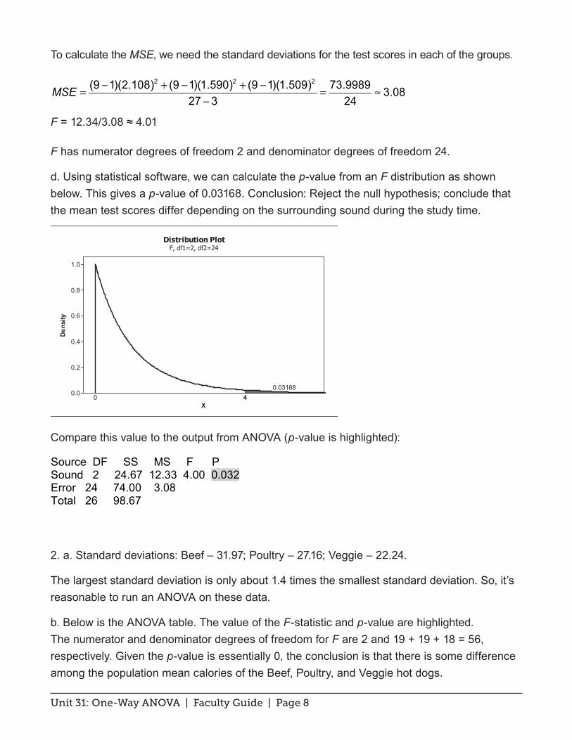
MSE = [(199)(9.164)2 + (199)(6.381)2 + (199)(6.933)2 + (199)(9.289)2]/(800 – 4) ≈ 51550.6/796 ≈ 64.762

F(3, 796) = 281.563/64.762 ≈ 4.35

d. Using software gives a p-value of around 0.005. (See distribution plot below.)

e. Not all of the population mean hourly pay rates for the four regions of the country are the same. The researchers could conclude that the mean hourly rate for the south is lower than the mean hourly rate for the northeast (since these two sample means are the farthest apart).

4. a.

b. The ratio of the largest standard deviation to the smallest standard deviation is 333.7/178.1, which is under 1.9. Hence, this assumption is reasonably satisfied.

c. Output from Minitab shown below.

0.8

0.7

0.6

0.5

0.4

0.3

0.2

0.1

0.0

X

Dens

ity

0.004741

0 4.35

Distribution PlotF, df1=3, df2=796

Occupation Sample Mean Standard Deviation

Cashier 424.9 178.1 Customer Service Representative 649.5 333.7 Receptionist 573.2 289.4 Secretary/Administrative Assistant 676.0 319.4

Review Question 4a


b. The ratio of the largest standard deviation to the smallest standard deviation is 333.7/178.1, which is under 1.9. Hence, this assumption is reasonably satisfied. c. Output from Minitab shown below. Source DF SS MS F P Factor 3 1907179 635726 7.73 0.000 Error 196 16112243 82205 Total 199 18019422 d. There are differences among the population mean weekly salaries among these four occupations. Based on the sample means, it appears that there is a difference in mean weekly wages between cashiers and secretaries/administrative assistants.


d. There are differences among the population mean weekly salaries among these four occupations. Based on the sample means, it appears that there is a difference in mean weekly wages between cashiers and secretaries/administrative assistants.

Documents

Prerequisites - learner.org · Additional coverage of ANOVA can be found in The Basic Practice of Statistics, Chapter 25, ... 0.35 0.40 0.45 0.50 0.55 0.60 0.65 0.70 4 3 2 1 0