1

Preschool and Maternal Labor Market Outcomes:

Evidence from a Regression Discontinuity Design*

Samuel Berlinski University College London and Institute for Fiscal Studies

Sebastian Galiani Washington University in St. Louis

Patrick J. McEwan Wellesley College

November 2008

*We thank Joseph Shapiro for his contributions to the paper. We further thank Phil Levine, Costas Meghir, Stephen

Nickell, Imran Rasul, and the referees and editors for their useful suggestions. Samuel Berlinski gratefully

acknowledges financial help from the ESRC-DFID grant RES-167-25-0124.

2

Abstract

In developing countries, employment rates of mothers with young children are relatively lower.

This paper analyzes how maternal labor market outcomes in Argentina are affected by the

preschool attendance of their children. Using pooled household surveys, we show that four year-

olds with birthdays on June 30 have sharply higher probabilities of preschool attendance than

children born on July 1, given enrollment-age rules. Regression-discontinuity estimates using

this variation suggest that preschool attendance of the youngest child in the household increases

the probability of full-time employment and weekly hours of maternal employment. We find no

effect of preschool attendance on maternal labor outcomes for children that are not the youngest

in the household.

JEL Codes: I21, I28, J22

Keywords: female labor supply, Argentina, regression-discontinuity, kindergarten.

3

I. Introduction

After World War II, female labor participation rates rose steadily in the developed and

developing world. However, participation rates in many countries are still relatively low for

mothers with young children. Not surprisingly, expanding preschool education is an oft-cited

goal in both developed countries (OECD 2002) and Latin America (Myers 1995; Schady 2006).

It provides an implicit child care subsidy, while also, perhaps, improving child outcomes (Blau

and Currie 2006). While a subsidy specifically designed to achieve one of these goals will

usually be relatively ineffective at accomplishing the other goal, the hope is that free public

preschool could attain both. Nonetheless, the empirical evidence on the effects of pre-primary

education is still limited, especially for developing countries.1

In two pertinent examples from South America, Berlinski, Galiani, and Gertler (forthcoming)

find a positive effect of pre-primary school attendance on the Spanish and Mathematics test

scores of Argentine third-graders, as well as behavioral outcomes such as attention, effort, class

participation, and discipline. Berlinski, Galiani, and Manacorda (2008), using data from the

Uruguayan household survey that collects retrospective information on preschool attendance,

find small gains in school attainment from preschool attendance at early ages that are magnified

with age. Less is known, however, about the effects of preschool on maternal labor market

outcomes.

A major challenge in identifying the causal effect of pre-primary school attendance on child

or parental outcomes is non-random selection into early education. To address this problem, our

1There is substantial empirical evidence from the United States that intensive early education interventions targeted

specifically to disadvantaged children yield benefits in the short and in the long run (Blau and Currie 2006). On the

less extensive evidence in Latin America, see Schady (2006).

4

paper uses the fact that Argentine children must reach a given age prior to a preschool enrollment

cutoff date. The school year runs from March to December, and enrollment in the final year of

preschool is mandatory for children that turn five years old by June 30. Children born on July 1

must wait one year to enroll in kindergarten. Using pooled household surveys that report exact

birth dates, we confirm that children born on July 1 have sharply lower probabilities, by about

0.3, of attending school. We exploit this discontinuity in the probability of attendance to identify

the effect of early school attendance on maternal labor market outcomes.

The parameters we study, however, differ from those of much research in the childcare and

female labor supply literature. Though many studies have estimated the sensitivity of maternal

employment to child care costs, their elasticity estimates cannot be easily generalized to predict

the effects of expanding preschool education on maternal labor market outcomes (Anderson and

Levine 2000; Blau and Currie 2006).2 Additionally, in the absence of credible instruments,

identification of the elasticities of maternal employment to childcare costs is challenging

(Browning 1992).

Our regression-discontinuity estimates suggest that, on average, 13 mothers start to work for

every 100 youngest children in the household that start preschool (though, in our preferred

specification, this estimate is not statistically significant at conventional levels). Furthermore,

mothers are 19.1 percentage points more likely to work for more than 20 hours a week (i.e., more

time than their children spend in school) and to work, on average, 7.8 more hours per week as a

consequence of their youngest offspring attending preschool. We find no effect of preschool

2 For the mothers that would work fewer hours than the school day, public schools provide a 100 percent marginal

price subsidy for childcare of fixed quality, while for the mothers that would otherwise work more hours the price

subsidy is inframarginal (Gelbach 2002).

5

attendance on maternal labor outcomes for children that are not the youngest in the household.

Finally, we find that at the point of transition from kindergarten to primary school there are

persistent employment effects, even though school attendance by then is nearly universal. This

might be explained by the fact that finding jobs takes time or by a mother’s decision to work

once the youngest child transitions to primary school.

Our preferred estimates condition on mother’s schooling and other exogenous covariates,

given evidence that mothers’ schooling is unbalanced in the vicinity of the July 1 cutoff in the

sample of four year-olds. Using a large set of natality records, we find no evidence that this is

due to precise birth date manipulation by parents. Other explanations, like sample selection, are

also not fully consistent with the data.

In terms of empirical strategies, Gelbach (2002) is the closest to the exercise we pursue in

this paper. He uses U.S. census data to estimate the effect of public school enrollment of five

year old children on their mothers’ labor market outcomes, instrumenting enrollment with

quarter of birth dummy variables. The idea is that the estimated parameters circumvent the

problems of endogenity mentioned above while being informative about whether large subsidies

in the form of limited, directly provided pre-primary education influence maternal labor

outcomes. A related literature from several countries reports difference-in-differences estimates

of preschool effects on maternal labor market outcomes, relying on geographic and temporal

variation in policies that affect preschool attendance.3

3 Cascio (forthcoming), exploits variation across the United States in the funding of kindergarten initiatives in the

late 1960s and early 1970s. She finds positive effects of kindergarten enrollment on maternal labor supply for single

mothers of five years-old with no younger children. Baker, Gruber and Milligan (2008) study the expansion of

subsidized provision of childcare for children zero to four in the Canadian province of Quebec. They also find that

childcare use has a positive effect on maternal labor supply for married mothers. Finally, Schlosser (2006) studies

6

Of particular relevance to this paper’s findings, Berlinski and Galiani (2007) examine an

Argentine infrastructure program, initiated in 1993, that built pre-primary classrooms for

children aged three to five. Using the fact that the construction exhibited variation in its intensity

across provinces, difference-in-differences estimates suggest that the take-up of new preschool

vacancies is perfect. The estimates further suggest that when a child is exogenously induced to

attend preschool by the supply expansion, the likelihood of maternal employment increases

between 7 and 14 percentage points, roughly similar to this paper’s point estimates. However,

Berlinski and Galiani only find a small, imprecisely estimated effect on hours worked.

The rest of the paper is organized as follows. Section II provides background information on

the education system in Argentina and describes the datasets used in this paper. Section III

describes our identification strategy. Section IV reports the empirical results, and section V

concludes.

II. Background and Data

A. Background Information

Argentina is a middle-income developing country with a long tradition of free public

schooling. The school system is divided into pre-primary, primary and secondary education.

Primary school attendance between 6 and 12 years old is virtually universal. However, the pre-

primary attendance rate among children aged 3 to 5 years old is only 64% in 2001 (Berlinski and

Galiani 2007). Pre-primary education is divided into three levels: level 1 (age 3), level 2 (age 4),

the impact on labor supply of the gradual implementation of compulsory preschool laws for children aged three to

four in Israel. She also finds that the provision of preschool education in Arab towns increases enrollment and

maternal labor supply.

7

and level 3 (age 5). In general, pre-primary classes are held within existing primary schools. Like

primary schools, they typically operate in separate morning and afternoon shifts, with children

attending one of these shifts for three and a half hours a day, five days a week, during a nine-

month school year.

Primary school has been compulsory since 1885. The Federal Education Law of 1993 further

mandated attendance between level 3 of pre-primary education and the second year of secondary

school. Its implementation was to have occurred gradually between 1995 and 1999, but it was

not rigidly enforced. First, there is no penalty in place for non-compliers. Second, primary school

enrollment is not impeded by lack of pre-primary schooling. Finally, there are still large dropout

rates at ages 13 and older.

In Argentina, the academic school year starts early in March and finishes in December. Like

many countries, a cutoff date establishes who can enroll in a given academic year. School age is

defined by the age attained on June 30 of the current academic year.4 Children can enroll in level

3 of preschool if they turn five years old on or before June 30 of the current school year.

Until 1994 Argentina was a relatively low unemployment country with unemployment rates

never exceeding 10 percent. However, unemployment increased substantially after a

macroeconomic shock in 1995 with an average rate of 14.5 for the rest of the nineties. Annual

hours worked are high and female participation is at the level of southern Europe. In 1998, the

female employment rate for the group aged 18 to 49 was 48 percent.

The Argentine labor market is not very rigid. Tax rates in Argentina are comparable to those

in a typical non-European OECD country. Unions are an important feature of economic life with

around half the workers having their wages bargained collectively and 45 percent of employees

4 See Art. 39, Resolución CABA: Nº 626/1980.

8

being union members. However, national minimum wages are set at a relatively low level and

probably do not have much impact on employment. Finally, employment protection is at about

the average OECD level (Galiani and Nickell 1999).

B. Data

We use data from the Argentine household survey, the Encuesta Permanente de Hogares

(EPH), a biannual survey of about 100,000 households managed by Argentina’s National

Institute of Statistics and Censuses (INDEC). The survey is representative of the urban

population of Argentina. It has been conducted since 1974 in the main urban clusters (referred to

as agglomerates) of each province of the country, with the exception of Rio Negro.5 A unique

feature of this household survey is that from May 1995 to May 2003 it includes the exact date of

birth for each individual in the sample. We pool repeated cross-sections of individual-level data

from both waves of the survey covering the 1995 to 2001 period. We do not use the information

for 2002 onwards because of the macroeconomic collapse of 2002 and its economic and

distributional consequences (Galiani et al. 2003; Mussa 2002).6

For our main results, we use a sample of households including mothers between the ages of

18 and 49 and at least one child aged 4 on January 1 of the survey year. The survey collects

information on the family relationship between household members and the head of household.

Our analysis focuses on children of either male or female household heads, because only in such

households can the mother of a child be identified in the EPH. We further restrict the sample to

5 Urban Rio Negro was included in the survey in 2001. See, www.indec.gov.ar for detailed information on the EPH.

6 GDP declined 20% and unemployment peaked at 24%. The results using the 1995 to 2003 sample are similar to

though less precise than those reported here and are available from the authors upon request.

9

individuals with full information on date of birth, school attendance, mother’s age and education,

and siblings’ ages. When children of the same household are born on the same day we only

include one of the children in the household.

In the first panel of Table 1 we summarize the information contained in the EPH sample. On

average, 58 percent of children aged 4 on January 1 of survey year attend school. However, the

enrollment rate was 81 percent for those born in the first half of the year and 33 percent for those

born on or after July 1. Thirty-seven percent of the mothers worked the previous week, with 30

percent working 20 or more hours per week (i.e., more time than their children spend in school).

The average number of hours worked last week is 12.17. The employment rate for the mothers of

children that attend preschool is 38 percent, versus 35 percent for those that do not. On average,

maternal characteristics such as age, education and labor market outcomes for the mothers of

children born in each half of the year are statistically similar.

We also use natality data from birth certificates, compiled by Argentina’s Ministry of

Health.7 It is not compulsory for provinces to report exact date of birth, but—with the exception

of the Province of Buenos Aires—all other provinces provide this information for the period

2002-2005.8 From this data we extracted all births to mothers aged 14-45 (i.e., those who will be

18-49 when their children turns 4). In the second panel of Table 1 we summarize the information

contained in the natality records.

III. Empirical Strategy

7 Further information can be found at the Dirección de Estadísticas e Información de Salud website:

http://www.deis.gov.ar/.

8 Natality data before 2002 do not contain exact date of birth.

10

This section describes the regression-discontinuity approach that we use to identify the effect

of preschool attendance on maternal labor market outcomes. It exploits sharp differences in the

probability of attendance for young children born on either June 30 or July 1. As a starting point,

consider the following linear model for a child aged 4 on January 1 of the survey year (i.e., a

child who is going to turn 5 in the calendar and academic year of the survey):

Yijs = αSijs + ′ β Xijs + λ j + µs + εijs (1)

where ijsY is a labor market outcome for the mother of child i, residing in region j, and observed

in survey round s (each survey round is the interaction of year and wave of the survey). ijsS is a

dummy variable indicating school attendance, ijsX is a vector of exogenous covariates that affect

maternal labor market outcomes, and ijsε is an error term assumed to be independent and

identically distributed. The model includes fixed effects for regions ( jλ ), equivalent to survey

“agglomerates”, and survey rounds (sµ ). The parameter of interest, α , represents the mean

effect of a child’s preschool attendance on the maternal labor market outcome.9 Because the

effects of preschool attendance on maternal labor outcomes could differ between households

whose youngest child enters kindergarten with respect to those who have younger children we

estimate separate models and parameters for these groups.

If we estimate the model in equation (1) by Ordinary Least Squares (OLS), the estimator of α

is likely to be inconsistent. First, maternal labor market outcomes and child’s school attendance

are jointly determined, introducing simultaneity bias. Second, omitted variables such as a

9 In the case of dichotomous measures of labor market outcomes, we also apply OLS and interpret coefficient

estimates as marginal probabilities.

11

mother’s cognitive ability are plausibly correlated with both labor outcomes and children’s

kindergarten attendance.

To disentangle the causal effect of preschool attendance, we use an instrument that induces

plausibly exogenous variation in ijsS , but has no direct effect on ijsY . In Argentina, children must

turn 5 years old on or before June 30 of the school year in which they enroll in (compulsory)

kindergarten. Those born one day later must wait a full year to enroll. Define a variable ijsB that

indicates a child’s day of birth during the calendar year. It equals -182 on January 1, 0 on July 1,

and 183 on December 31. Further defineZijs =1 Bijs ≥ 0{ }, an indicator function which equals to

one for children born on or after July 1, and zero otherwise.

We model school attendance using a linear probability model:

ijssjijsijsijsijsijsijsijsijs BZBZBBZS υµλδδδδδ +++×+×+++= 243

2210 (2)

The parameter 0δ measures the discontinuity in preschool attendance on July 1. In our sample

of Argentine 4 year-olds, we anticipate that 00 <δ , since children born on or after July 1 do not

fulfill the minimum age requirement for enrollment in kindergarten. In practice, the point

estimate is likely to be greater than -1 (a so-called “fuzzy” discontinuity), since younger children

may already be enrolled in the previous, non-compulsory level of preschool, and some older

children may ignore compulsory attendance rules.

Similarly, we can model maternal labor market outcomes as

Yijs = α0Zijs + α1Bijs + α2Bijs2 + α3Zijs × Bijs + α4Zijs × Bijs

2 + λ j + µs + ηijs (3)

where α0 captures the reduced-form effect of July 1 birthdays on labor outcomes. Since we

anticipate that 10 −>δ , the estimate of 0α must be rescaled by the estimate of 0δ to recover the

effect of school attendance on labor outcomes. In practical terms, this parameter is computed by

12

estimating equation (1) via two-stage least squares (TSLS), conditioning on the interacted

polynomials of ijsB and instrumenting Sijs with ijsZ (see, e.g., van der Klaauw 2002; Imbens and

Lemiuex 2008).

For this to identify the parameter of interest, ijsZ must be correlated with ijsS , but it should

not have a direct effect on the outcome of interest, i.e. 0),cov( =ijsijsZ ε . Since parents can time

conception, a child’s season of birth is plausibly correlated with unobserved variables like child

health and family income, any of which could directly influence maternal labor market outcomes

(Bound, Jaeger, and Baker 1995; Bound and Jaeger 2000). To address this, the TSLS

specifications control for smooth functions of ijsB , estimated separately on either side of the

cutoff date.10 The specification above assumes a piecewise quadratic polynomial, but we verify it

through visual inspection of means taken within day-of-birth cells, in addition to obtaining

estimates with higher-order polynomials.

Although the polynomials capture smooth, seasonal differences in birth date manipulation,

they cannot capture precise manipulation, near the cutoff date, via cesarean sections or induced

births. In the next section, we use natality data from birth certificates to show that this is an

unlikely source of bias. Another possible threat to the internal validity of our estimates could

come from welfare subsidies varying with school age. In this scenario, we could confound the

effect of preschool attendance with the effect of these subsidies. To our knowledge, in Argentina,

no such overlapping discontinuities exist in the design of the welfare system. Finally, parents

10 The estimated regression functions do not fully saturate the model. Lee and Card (2008) show that one can

interpret the deviation between the true conditional expectation function and the estimated regression function as

random specification error that introduces a group structure into the standard errors for the estimated treatment

effect. Thus, we always report standard errors clustered by 366 days of birth.

13

may deceive educational authorities about their child’s date of birth in order to enroll them in

preschool earlier. This practice is difficult to implement in Argentina, since enrollment requires a

national identification card that includes the officially-recorded date of birth. Moreover, this

would only constitute a threat to internal validity if parents lie to the household survey about

birth dates (in addition to the school authorities), which they have no incentive to do.

The interpretation of the TSLS estimates requires some clarification.11 Under a weak

monotonicity assumption, as in Imbens and Angrist (1994), the estimates are informative about

the behavior of compliers (i.e. the subgroup of individuals whose treatment status switches from

nonrecipient to recipient if their birth date crosses the cut-off).12 Our analysis includes children

that will turn 5 years old during the academic year. In this sample, the subgroup of non-

compliers includes households that choose to send their children to preschool for two years or

more, and thus are not influenced by the cutoff date. In contrast, the compliers include

households that choose only one year of preschool. Thus, our estimates are most generalizable

to households that choose less preschool, perhaps likely to be poorer and credit constrained, or

with less access to preschool infrastructure.

IV. Main Results

11 One interpretation for the parameters we estimate is that of an equivalent cash childcare subsidy. We find this

interpretation less straightforward as preschool education as a means of childcare imposes fixed costs on parents

(e.g., children have to be taken and collected from school at certain times) that a childcare cash subsidy may not.

Parents likely also value the learning of children during pre-primary education. Finally, the population that would be

affected by these two conceptual experiments might be different.

12 For a complete discussion of the fuzzy regression-discontinuity design, see Hahn, Todd, and van der Klaauw

(2001) and Imbens and Lemieux (2008).

14

A. Evidence on Birth Timing

We investigate the validity of our identifying assumption by examining whether there is

manipulation of the assignment variable, perhaps via cesarean section or induced labor.13 It is

plausible in Argentina, where one-quarter of births are via cesarean section, with rates between

36 and 45 percent in private hospitals (Belizán et al. 1999). Presuming that timed births do not

occur from a random draw of the population, it is plausible that the clustering of such parents just

to the left (or right) of the July 1 cutoff could introduce a correlation between ijsZ and ijsε .

We use two strategies to diagnose systematic manipulation of the assignment variable

(Imbens and Lemieux 2008; Lee 2008). First, we examine the density of birthdates around the

July 1 cutoff for clustering on either side of the cutoff. Second, we examine the distribution of

observed socioeconomic and birth characteristics around the enrollment cutoff, interpreting sharp

changes in these variables as suggestive of nonrandom birth date manipulation.

Figure 1 reports a histogram of births using large samples from the natality data. Black bars

indicate the July 1 cutoff, as well non-floating holidays in Argentina, given evidence that birth

frequencies are lower on such days. There is a strong case that families are capable of precisely

timing births (McEwan and Shapiro 2008). The upper-left panel shows proportionally fewer

births on weekends, and that mothers of such births have less schooling. This pattern, common

across many countries, has been shown to be correlated with the use of cesarean sections and

induced labor (Dickert-Conlin and Chandra 1999). To determine whether such birth timing

13 In Chile, with a similarly high rate of cesarean sections (Belizán et al. 1999), McEwan and Shapiro (2008) found

no evidence of birth timing around a July 1 enrollment cutoff. In the U.S., McCrary and Royer (2006) find no

evidence of sorting around birthdate cutoffs in Texas and California. In other countries, evidence suggests that

parents have manipulated birth dates in order to avoid taxes (Dickert-Conlin and Chandra 1999) and obtain

monetary bonuses (Gans and Leigh Forthcoming).

15

might occur around July 1, the upper-right panel reports a histogram of all births. Because of the

large sample, we restrict it to a 6-month window around July 1, but the results are robust to a

larger window. While there are visible dips in births on three national holidays, consistent with

the ability to time births, there is no evidence of clustering of births on either side of July 1.

In the bottom panels of Figure 1, we summarize the relationship between birth dates and two

variables: weeks of gestation and mother’s schooling. The circles represent the unadjusted means

of these variables within daily cells. The superimposed lines are fitted values from a piecewise

quadratic specification on date of birth. There is, interestingly, evidence that declines in birth

frequencies on holidays are associated with lower values of mothers’ schooling (indicated by the

solid dots). However, there is no visual evidence of breaks around July 1.

In Table 2, we present OLS regression results that are the analogue of the visual evidence in

the bottom panels of Figure 1. This table confirms the finding of no differences in gestation and

schooling near the July 1 cutoff. It shows similar results for a larger set of covariates that

include low birth weight. In sum, the natality data provide no evidence of systematic

manipulation of birth dates around the July 1 cutoff.

B. Day of Birth, Preschool Attendance, and Covariate Smoothness

We turn now to the analysis of preschool attendance and covariate smoothness using the EPH

sample. In Figure 2, we summarize the relationship between birth date and preschool attendance.

The top panels present results among 3 and 4 year-olds who are the youngest in the household,

and the bottom panels among those that are not the youngest in the household. (In this and all

subsequent analyses, children’s age is calculated on January 1 of the survey year in which they

16

are observed.) The circles represent unadjusted means of the school attendance variable within

daily cells. The superimposed lines are fitted values from a piecewise quadratic specification.

Figure 2 shows, as expected, that preschool attendance is low among 3 year-olds. There is a

small break in attendance, with children born on or just after July 1 slightly less likely to attend

than children born just before. A larger break is evident among 4 year-olds, consistent with the

fact that kindergarten (i.e., level 3 of preschool) is compulsory. Four year-olds born on July 1 are

just below the minimum age requirement for kindergarten and must delay enrollment by one

year, while 4 year-olds born on June 30 are eligible to enroll as the youngest kindergarteners.

Table 3 reports OLS estimates of equation (2), the empirical analogue of Figure 2. Panel A

presents the results for the youngest children in the household, and Panel B the results for

children who are not the youngest in the household.14 In column (1) of Panel A, where we only

condition on a piecewise quadratic polynomial, we find that among 4 year-olds, the coefficient

on birthdays after June 30 is a large, negative, and highly significant estimate of -0.31. It is much

smaller (-0.048) among 3 year-olds, albeit significant. In column (2), we add a full set of

controls, including dummy variables for each survey round, regional agglomerate, day of week

of birthday, birthdays on non-floating holidays,15 linear and quadratic terms of mother’s age, a

dummy variable indicating female children, and dummies for mother’s years of schooling. The

results are not statistically different than those reported in Column (1). The results for the sample

14 A regression of a youngest in the household dummy on a born on/after July 1 dummy and a piecewise quadratic

polynomial shows no correlation between being the youngest in the household and the July 1 dummy.

15 We include these variables to show that the results are not driven by coincidental overlap of cutoff dates falling on

weekends or holidays. Nevertheless, the results reported in the paper are very similar if we do not include these

control variables.

17

of children that are not the youngest in the households are similar, suggesting that this aspect of

family structure does not affect compliance with the enrollment rule.

Before examining the effect of preschool attendance on maternal labor outcomes, we

scrutinize whether, in the EPH sample, covariates are smooth around the cutoff point. In Table 4,

we report successive OLS estimates of an equation like (3) for mother’s age, years of schooling,

and a dummy variable indicating whether the child is female. Panel A refers to the sample of

children who are the youngest in the household, and Panel B to the sample of children who are

not. The most obvious pattern is that mother’s schooling is systematically lower among the

youngest children in each household born on or after July 1 (that is, among children less likely to

attend school). The basic result is robust to the inclusion of dummy variables for agglomerates,

surveys, day-of-week of birth, and holiday births. Interestingly, mother’s schooling is balanced

around the cutoff for the sample of children that are not the youngest in the household and for

those children aged 3. In Figure 3, we present the corresponding visual evidence for mother’s

schooling.

In Table 5, we present a number of robustness checks, both for the results on preschool

attendance and mother’s schooling. For brevity, we focus on the sample of 4 year-olds. We start

by examining whether the quadratic specification is driving our results. Column (1) is the

benchmark; for preschool attendance we reproduce the estimates of column (2) in Table 3, with

the full set of controls, and for mother’s schooling those of column (5) in Table 4.16 In columns

(2) and (3), we respectively include cubic and quartic piecewise polynomials. In the remaining

columns, we use a piecewise quadratic polynomial but within different samples. In column (4),

16 The results for the mother’s schooling equations are similar if we include other controls and use as the benchmark

column (6) of Table 4.

18

we focus on the sample of children born between April and September. In column (5), we drop a

one week window at both sides of the cutoff. In column (6), we use survey weights. None of

these changes in the specification of the analysis affects the basic results we have presented so

far.

In the final two columns of Table 5, we present the results of a placebo experiment. In

column (7), we take the sample of children born between January 1 and June 30. We center the

date of birth variable on April 1 and we create a dummy for being born on or after April 1 that

we interact with a quadratic polynomial. We report the coefficient of this dummy variable. In

column (8), we conduct a similar exercise for those children born between July 1 and December

31. The dummy variable is now being born on or after October 1. We find no statistically

significant correlations between the outcomes and these dummy variables. However, it is worth

noting that the coefficient on mother’s years of schooling can be large (the p-value is 0.115) as

the result in column (7) shows.

The fact that covariates are smooth around July 1 in the natality data reduces the plausibility

of systematic manipulation of birth dates as an explanation for the robust correlations just

observed. One alternative explanation is sample selection. This could happen, for example, if

relatively less-educated mothers of children born before July 1 are induced to work more than

the mothers of children born on or after July 1, and also are less likely to be interviewed by the

household survey as a result. Though a potentially compelling explanation, the point estimates

are large enough to render it less plausible. On average, the mothers of children age 4 completed

9.37 years of education with 64.4% of these mothers completing 9 or less years of education.17

17 The distribution of years of education for the mothers of children age 4 is: 0 (0.85%), 3 (11.16%), 7 (30.00%), 9

(22.53%), 12 (16.74%), 14 (2.29%), 15 (11.46%) and 17 (5.08%).

19

Suppose that the mothers with less than the average level of education are selecting out of the

sample at the same rate over the whole education distribution. In this case, we need

approximately 38% of these mothers to disappear from the sample to generate a difference of 0.8

years of education.18

Furthermore, we find large differences in schooling among the mothers of the non-youngest

children aged 1 and 2 years old (the results are not reported in the tables). Almost none of these

children attend school, so it is unlikely to result from labor-supply induced sample selection. As

it stands, the most likely explanation is noise, though we cannot rule out the presence of sample

selection. As a result, our preferred estimates in the next section control for mothers’ schooling.

The unconditional instrumental variables estimates will likely be biased upwards because of the

positive correlation between education and labor market outcomes. Of course, to the extent that

selection on unobservables is plausible, our results might still be biased, although the direction of

the bias is not clear.

C. School Attendance and Maternal Labor Outcomes

In Table 6, we report estimates from reduced-form regressions of mother’s labor market

outcomes on a dummy variable indicating births on or after July 1. The variables include whether

mothers were employed last week, whether mothers worked for at least 20 hours last week (“full-

time”), and the number of hours worked last week. We estimate separate OLS regressions of

equation (3) for children aged 3 and 4. All regressions control for a piecewise quadratic of birth

18 The distribution of years of education if 38 percent of the mothers with less than 9.317 years of education drop out

from the sample would be: 0 (0.70%), 3 (9.08%), 7 (24.63%), 9 (18.50%), 12 (22.17%), 14 (3.03%), 15 (15.18%)

and 17 (6.73%). Therefore, average years of education is 10.166.

20

date, while regressions in even columns include a full set of controls. Because children born on

or after July 1 are less likely to attend school, we expect a negative effect for maternal labor

outcomes of being born on or after July 1.

In the samples of 3 year-olds, none of the coefficients are statistically distinguishable from

zero. This is perhaps not surprising given the relatively small difference in school attendance

around the July 1 cutoff for such children. For children aged 4 that are the youngest in the

household, the coefficients in Table 6 range between -0.066 and -0.038 when a dichotomous

indicator of mother’s employment is the dependent variable. Coefficients range between -0.085

and -0.058 when the dependent variable is work for more than 20 hours a week. In columns (5)

and (6), mothers of children born in the second semester of the year work between 2.4 and 3.4

less hours in the previous week. Not surprisingly, given the evidence from the previous section,

the coefficients from fully-specified models are less negative. The pattern of the reduced-form

results just described is corroborated in Figure 4, which presents unsmoothed means and fitted

values for children aged 4, for the youngest children (upper panels) and not youngest (lower

panels).

Despite the fact that there is a significant increase in preschool attendance among children

aged 4 that are not the youngest in the household, there is no evidence of changes in employment

or hours of work for their mothers. In theory, it is plausible that there could be an effect on these

outcomes for the mothers of these children as the childcare provided by preschool attendance of

at least one of their children contributes towards reducing the total cost of childcare. However,

the result implies that this contribution is small relative to the cost of childcare for the other

children and does not affect the decision of the mother to either work or work for more hours.

21

Table 7 reports two-stages least squares estimates, which are simply the reduced-form

estimates from Table 6 divided by the changes in the probability of attendance estimated among

4 year-olds in Table 3. Among the sub-sample of youngest children (panel A), the model with

the full set of controls suggests that mothers with children attending kindergarten are 12.7

percentage points more likely to work, though the estimate is not precise. This means that 13

mothers start working for every 100 youngest children in the household that start preschool.

Furthermore, mothers are 19.1 percentage points more likely to work more than 20 hours per

week, and they work, on average, 7.8 more hours per week as consequence of their youngest

child attending preschool. Both estimates are statistically significant at the 10 percent level. The

point estimates of the binary employment measures are consistent with the upper end of

estimates reported in Berlinski and Galiani (2007), who used a different EPH sample and an

empirical strategy using temporal and regional variation in preschool construction.

In Table 8, we report a set of robustness checks for the two-stages least squares estimates.19

Column (1) is the benchmark, reproducing estimates from columns (2), (4) and (6) in Table 7. In

columns (2) and (3), we use cubic and quartic polynomials respectively. In the remaining

columns of Table 5, we use a piecewise quadratic polynomial but within different samples. In

column (4), we focus on the sample of children born between April and September. In column

(5), we drop a one-week window on each side of the cutoff. In column (6), we use survey

19 We have also estimated the effect of preschool attendance on maternal labor outcomes using locally weighted

regressions (results available upon request from the authors). The estimates for the youngest in the household are

similar in magnitude to those presented in Table 7 and robust to the choice of bandwidth. However, they are

imprecisely estimated. For children who are not the youngest in the household the magnitude of the estimates tend to

be positive but are quite sensitive to the bandwidth choice and are also imprecisely estimated.

22

weights.20 The results in Panel A are similarly-signed, but less precise than in the benchmark

specification. The most noticeable difference is that when we weight observations using the

survey weights, the results for the non-youngest children in the household (panel B) tend to be

similar to the results for the youngest children.

D. Heterogeneous Effects

We have shown that the effect of the enrollment rule on preschool attendance is not affected

by whether there are younger siblings in the household. However, the maternal labor market

response to the preschool enrollment rule for 4 year old children is remarkably different for the

mothers of children with and without younger siblings. We next explore whether other variables

that are likely to affect maternal home and market productivity, such as age and schooling,

impact their behavioral responses to the enrollment rule.

In Table 9, we report estimates from OLS regressions of school attendance, mother’s

schooling, mother’s employment, employment for more than 20 hours last week, and hours

worked last week on a dummy variable indicating births on or after July 1 for four samples of 4

year old children: mothers aged 35 or older, mothers younger than 35 years of age, mothers with

incomplete high school or lower educational achievement, and mothers with complete high

school education or higher educational achievement. All regressions control for a piecewise

quadratic of birth date, while regressions in even columns include a full set of controls. Panel A

present results for children that are the youngest in the household and panel B for other children.

20 Because in the placebo experiments from Table 5 the effect on attendance is close to zero, the corresponding two-

stage least squares estimates are close to zero as well.

23

We find that effect of the enrollment rule on preschool attendance is not significantly

different between children with mothers of different ages. There is some evidence that the

preschool attendance of youngest children in the household with mothers that have lower

education is more sensitive to the enrollment rule–about 6 percentage points–but this difference

is not statistically significant. The lack of balancing on maternal education persists for the

youngest children in the household regardless of their mothers’ age group. Dividing the sample

by maternal education seemingly resolves the lack of balancing in maternal education around the

cutoff. However, this appears to be a mechanical consequence of censoring the dependent

variable, and does not provide any goods news for identification.

In terms of labor market responses, the effects are still concentrated among mothers for

whom the child is the youngest in the household. Despite the fact that the enrollment rule

produces similar responses in term of preschool attendance for the different groups, we find that

the effects on employment and hours of work are driven by older and less educated mothers. For

example, among the sub-sample of youngest children (panel A), the model with the full set of

controls suggests that mothers with children born on or after July 1 were 8.4 percentage points

less likely to work, 11 percentage points less likely to work full time, and worked 5 hours less

per week. This is equivalent to an effect of preschool attendance on employment of 19

percentage points, on full-time work of 23 percentage points, and on hours work of 11.65

hours.21 We speculate that older mothers with young children are either less likely to have

additional children or have more attachment to the labor market, and thus are more responsive

when their youngest child starts preschool. In the absence of a comprehensive welfare system, as

21 Instrumental variables results available from the authors upon request.

24

in Argentina, less-educated mothers may also have the need to return to work as soon as it is

feasible.

E. Day of Birth and Maternal Outcomes for Primary School Children

In Table 10, we reproduce estimates for school attendance, mother’s schooling, mother’s

employment, employment for more than 20 hours last week, and hours worked last week for

children aged 5 and 6 on July 1 of the survey year. School enrollment is uniformly high at these

ages and there is no enrollment effect of July 1 births. The correlation between maternal

schooling and being born in the second semester still persists. We find that for children aged 5

that are the youngest in the household the maternal labor outcomes coefficients in Table 10 tend

to be of similar sign and magnitude than those of the youngest children aged 4 we reported in

Table 6. We find no systematic effects for children aged 6 or for those children that are not the

youngest in the household.

Why do we observe employment effects for children aged 5 when there is no school

attendance discontinuity? One explanation is that the result is an statistical artifact reflecting a

lack of balancing in the observables. Although this is theoretically plausible, it does not explain

why, in our sample, such a correlation does not exist at age 6. An alternative explanation is that

although some mothers find employment at the moment when their children start kindergarten,

for others it takes time to find suitable employment so that some effects appear at age 5. Given

the similarity in the magnitude of the coefficients between ages 4 and 5, one suspects that this

cannot be the whole story. A complementary explanation is that, at age 5, the dummy for being

born on or after July 1 picks up the difference between being enrolled in kindergarten and

primary school. If the maturity of a child plays a role on the decision of a mother to go work, the

25

transition from kindergarten to primary school may be interpreted by families as a signal that in-

home care is no longer necessary.22 This is consistent with the fact that no such effect appears at

age 6.

V. Conclusion

Expanding preschool education has the dual goals of improving child outcomes and work

incentives for mothers. This paper provides evidence on the second, identifying the impact of

preschool attendance on maternal labor market outcomes in Argentina. A major challenge in

identifying the causal effect of preschool attendance on parental outcomes is non-random

selection into early education. We address this by relying on plausibly exogenous variation in

preschool attendance that is induced when children are born on either side of Argentina’s

enrollment cutoff date of July 1. Because of enrollment cutoff dates, 4 year-olds born just before

July 1 are 0.3 more likely to attend preschool. Our regression-discontinuity estimates compare

maternal employment outcomes of 4 year-old children on either side of this cutoff, identifying

effects among the subset of complying households (who are perhaps more likely to face

constraints on their level 2 preschool attendance).

Our findings suggest that, on average, 13 mothers start to work for every 100 youngest

children in the household that start preschool (though, in our preferred specification, this

estimate is not statistically significant at conventional levels). Furthermore, mothers are 19.1

percentage points more likely to work for more than 20 hours a week (i.e., more time than their

children spend in school) and they work, on average, 7.8 more hours per week as consequence of

22 A more practical explanation is that primary schools may have longer school days and hence provide a larger

implicit subsidy. Nevertheless, primary schools, like preschools, also operate mainly on a two-shift schedule.

26

their youngest offspring attending preschool. We find no effect on maternal labor outcomes

when a child that is not the youngest in the household attends preschool. Finally, we find that at

the point of transition from kindergarten to primary school some employment effects persist.

Our preferred estimates condition on mother’s schooling and other exogenous covariates,

given evidence that mothers’ schooling is unbalanced in the vicinity of the July 1 cutoff in the

sample of 4 year-olds. Using a large set of natality records, we found no evidence that this is due

to precise birth date manipulation by parents. Other explanations, like sample selection, are also

not fully consistent with the data, and we must remain agnostic on this point. Despite this

shortcoming, the credibility of the estimates is partly enhanced by the consistency of point

estimates with Argentine research using a different EPH sample and sources of variation in

preschool attendance (Berlinski and Galiani 2007).

A growing body of research suggests that pre-primary school can improve educational

outcomes for children in the short and long run (Blau and Currie 2006; Schady 2006). This paper

provides further evidence that, ceteris paribus, an expansion in preschool education may enhance

the employment prospects of mothers of children in preschool age.23

23 However, as a referee notes, the large-scale expansion of preschool might have additional effects not reflected in

our empirical results. For example, one could imagine that it increases fertility, which could have countervailing

effects on labor supply among women.

27

References

Anderson, Patricia M., and Philip B. Levine. 2000. “Child Care and Mothers’ Employment

Decisions.” In Finding Jobs: Work and Welfare Reform, ed. David Card and Rebecca M.

Blank. New York: Russell Sage Foundation.

Baker, Michael, Jonathan Gruber, and Kevin Milligan. 2008. “Universal Childcare, Maternal

Labor Supply and Family Well-Being.” Journal of Political Economy 116: 709-45.

Belizán, José M., Fernando Althabe, Fernando C. Barros, and Sophie Alexander. 1999. “Rates

and Implications of Caesarean Sections in Latin America: Ecological Study.” British Medical

Journal 319: 1397-400.

Berlinski, Samuel, and Sebastian Galiani. 2007. “The Effect of a Large Expansion of Pre-

Primary School Facilities on Preschool Attendance and Maternal Employment.” Labour

Economics 14: 665-80.

Berlinski, Samuel, Sebastian Galiani, and Paul Gertler. Forthcoming. “The Effect of Pre-Primary

Education on Primary School Performance.” Journal of Public Economics.

Berlinski, Samuel, Sebastian Galiani, and Marco Manacorda. 2008. “Giving Children a Better

Start: Preschool Attendance and School-Age Profiles.” Journal of Public Economics 92:

1416-40.

Blau, David, and Janet Currie. 2006. “Pre-School, Day Care, and After School Care: Who’s

Minding the Kids?” In Handbook of the Economics of Education (vol. 2), ed. Eric Hanushek

and Finis Welch. Amsterdam: Elsevier.

Bound, John, and David A. Jaeger. 2000. “Do Compulsory Attendance Laws Alone Explain the

Association Between Earnings and Quarter of Birth?” In Research in Labor Economics:

Worker Well-Being, ed. Solomon W. Polacheck. New York: JAI.

28

Bound, John, David A. Jaeger, and Regina M. Baker. 1995. “Problems with Instrumental

Variables Estimation When the Correlation Between the Instruments and the Endogenous

Explanatory Variable is Weak.” Journal of the American Statistical Association 90: 443-50.

Browning, Martin. 1992. “Children and Household Economic Behavior.” Journal of Economic

Literature 30: 1434-75.

Cascio, Elizabeth. Forthcoming. “Maternal Labor Supply and the Introduction of Kindergartens

into American Public Schools.” Journal of Human Resources.

Dickert-Conlin, Stacy, and Amitabh Chandra. 1999. “Taxes and the Timing of Births.” Journal

of Political Economy 107: 161-77.

Galiani, Sebastian, Daniel Heymann, and Mariano Tommasi. 2003. “Great Expectations and

Hard Times: The Argentina Convertibility Plan.” Economía 4: 109-60.

Galiani, Sebastian, and Stephen Nickell. 1999. “Unemployment in Argentina in the 1990s.”

Working Paper DTE 219, Instituto Torcuato Di Tella.

Gans, Joshua S., and Andrew Leigh. Forthcoming. “Born on the First of July: An (Un)natural

Experiment in Birth Timing.” Journal of Public Economics.

Gelbach, Jonah B. 2002. “Public Schooling for Young Children and Maternal Labor Supply.”

American Economic Review 92: 307-22.

Hahn, Jinyong, Petra Todd, and Wilbert van der Klaauw. 2001. “Identification and Estimation of

Treatment Effects with a Regression-Discontinuity Design.” Econometrica 69: 201-9.

Imbens, Guido W., and Joshua D. Angrist. 1994. “Identification and Estimation of Local

Average Treatment Effects.” Econometrica 62: 467-75.

Imbens, Guido W., and Thomas Lemieux. 2008. “Regression Discontinuity Designs: A Guide to

Practice.” Journal of Econometrics 142: 615-35.

29

Lee, David S. 2008. “Randomized Experiments from Non-Random Selection in U.S. House

Elections.” Journal of Econometrics 142: 675-97.

Lee, David S., and David Card. 2008. “Regression Discontinuity Inference with Specification

Error.” Journal of Econometrics 142: 655-74.

McCrary, Justin, and Heather Royer. 2006. “The Effect of Maternal Education on Fertility and

Infant Health: Evidence from School Entry Laws Using Exact Date of Birth.” Unpublished

manuscript, University of Michigan and Case Western.

McEwan, Patrick J., and Joseph S. Shapiro. 2008. “The Benefits of Delayed Primary School

Enrollment: Discontinuity Estimates Using Exact Birth Dates.” Journal of Human Resources

43: 1-29.

Mussa, Michael. 2002. Argentina and the Fund. From Triumph to Tragedy. Washington, DC:

Petersen Institute.

Myers, Robert J. 1995. “Preschool Education in Latin America: Estate [sic] of practice.”

Working Paper No. 1, PREAL, Washington, DC.

OECD. 2002. “Strengthening Early Childhood Programs: A Policy Framework.” In Education

Policy Analysis, Paris.

Schady, Norbert. 2006. “Early Childhood Development in Latin America and the Caribbean.”

Economía 6: 185-225.

Schlosser, Analía. 2006. “Public Preschool and the Labor Supply of Arab Mothers: Evidence

from a Natural Experiment.” Unpublished manuscript, Hebrew University of Jerusalem.

van der Klaauw, Wilbert. 2002. “Estimating the Effect of Financial Aid Offers on College

Enrollment: A Regression-Discontinuity Approach.” International Economic Review 43:

1249-87.

All

Birth

days

Birth

days

7/1

or

earlie

ron 7

/1 o

r la

ter

-0.4

0-9

2.3

091.2

1

(105.9

2)

(52.6

3)

(53.2

1)

Born

on/a

fter

cuto

ff0.5

00

10/1

22,9

74

Attends s

chool

0.5

80.8

10.3

30/1

22,9

74

Fem

ale

0.4

80.4

80.4

90/1

22,9

74

32.8

133.0

432.5

8

(6.2

4)

(6.2

4)

(6.2

3)

9.3

79.3

59.4

0

(3.9

0)

(3.8

6)

(3.9

4)

Moth

er

work

s0.3

70.3

70.3

70/1

22,9

74

Definitio

nM

ean (

Sta

ndard

devia

tion)

Min

imum

/

Maxim

um

N

Panel A

: E

ncuesta

Perm

anente

de H

ogare

s, M

ay 1

995 to O

cto

ber

2001 (

4 y

ear-

old

s)

Birth

day

Child

's d

ay o

f birth

in the c

ale

ndar

year,

defined

to a

ddre

ss leap y

ears

: 1/1

=-1

82; 7/1

=0;

12/3

1=

183.

-182/1

83

22,9

74

Child

's d

ay o

f birth

is 7

/1 o

r la

ter.

Child

attended a

ny level of school at tim

e o

f

surv

ey.

Child

is fem

ale

.

Moth

er’s a

ge

Moth

er’s a

ge in d

ecim

al years

.18.0

1/4

9.9

422,9

74

Moth

er’s s

choolin

gM

oth

er’s y

ears

of fo

rmal schoolin

g.

0/1

722,9

74

Moth

er

work

ed last w

eek.

Ta

ble

1: V

ari

ab

le D

efin

itio

ns a

nd

De

scri

ptive

s S

tatistics

Moth

er

work

s full-

tim

e0.3

00.3

00.3

00/1

22,8

41

12.1

712.0

812.2

7

(19.0

5)

(19.0

3)

(19.0

6)

-0.1

4-4

5.4

545.7

8

(53.1

8)

(26.2

4)

(26.7

2)

Born

on/a

fter

cuto

ff0.5

00

10/1

888,0

33

Satu

rday

0.1

20.1

20.1

20/1

888,0

33

Sunday

0.1

00.1

00.1

00/1

888,0

33

Holid

ay

0.0

10.0

20.0

10/1

888,0

33

26.3

726.4

126.3

4

(6.5

0)

(6.5

0)

(6.5

0)

9.3

69.3

39.4

0

(3.8

4)

(3.8

4)

(3.8

4)

Low

birth

weig

ht

0.0

70.0

70.0

70/1

877,5

51

38.7

838.7

838.7

8

(1.8

9)

(1.8

9)

(1.8

9)

Public

facili

ty0.5

80.5

80.5

80/1

886,9

09

Liv

es w

ith p

art

ner

0.8

40.8

40.8

40/1

864,8

79

Moth

er

work

ed 2

0 o

r m

ore

hours

last w

eek.

Hours

work

ed

Moth

er’s h

ours

work

ed in a

ll jo

bs last w

eek.

0/8

422,8

41

Panel B

: N

ata

lity file

s, 2002-2

005

Birth

day

Sam

e a

s a

bove.

-91/9

1888,0

33

Sam

e a

s a

bove. B

orn

on S

atu

rday.

Born

on S

unday.

Born

on a

non-f

loating h

olid

ay:

1/1

, 1/5

, 25/5

, 9/7

, 8/1

2, 24/1

2, 25/1

2, 31/1

2

Moth

er’s a

ge

Moth

er’s a

ge in inte

ger

years

.14/4

5888,0

33

Moth

er’s s

choolin

gM

oth

er's y

ears

of fo

rmal schoolin

g.

0/1

6874,9

04

Moth

er

lives w

ith a

part

ner.

Birth

weig

ht is

less than 2

500 g

ram

s.

Gesta

tion

Weeks o

f gesta

tion.

14/4

5857,3

30

Child

born

in a

public

health facili

ty.

No

tes: T

he

En

cu

esta

Pe

rma

ne

nte

de

Ho

ga

res s

am

ple

(P

an

el A

) in

clu

de

s c

hild

ren

fro

m s

urv

eys b

etw

ee

n M

ay 1

99

5 a

nd

Octo

be

r 2

00

1

wh

o w

ere

4 y

ea

rs-o

ld o

n J

an

ua

ry 1

of su

rve

y y

ea

r a

nd

ha

d a

mo

the

r p

rese

nt a

ge

d 1

8-4

9. T

he

na

talit

y file

s (

Pa

ne

l B)

inclu

de

bir

ths fro

m

the

20

02

-20

05 file

s, o

f m

oth

ers

ag

ed

14

-45

th

at o

ccu

rre

d b

etw

ee

n A

pri

l 1

an

d S

ep

tem

be

r 3

0.

Moth

er's

Moth

er's

Low

Birth

Gesta

tion

Public

Liv

es w

ith

schoolin

gage

weig

thfa

cili

typart

ner

(1)

(2)

(3)

(4)

(5)

(6)

Born

on/a

fter

cuto

ff0.0

22

0.0

87*

-0.0

01

0.0

12

-0.0

03

0.0

01

[0.0

25]

[0.0

51]

[0.0

02]

[0.0

15]

[0.0

04]

[0.0

02]

Sunday

-0.5

17**

*-0

.944**

*0.0

06**

*0.0

11

0.1

05**

*-0

.025**

*

[0.0

19]

[0.0

36]

[0.0

01]

[0.0

10]

[0.0

03]

[0.0

01]

Table

2: D

ay o

f B

irth

and B

aselin

e V

ariable

s,

Nata

lity D

ata

[0.0

19]

[0.0

36]

[0.0

01]

[0.0

10]

[0.0

03]

[0.0

01]

Satu

rday

-0.2

95**

*-0

.633**

*0.0

07**

*-0

.008

0.0

60**

*-0

.018**

*

[0.0

19]

[0.0

34]

[0.0

01]

[0.0

08]

[0.0

03]

[0.0

02]

Holid

ay

-0.3

22**

*-0

.377**

*0.0

01

0.0

26**

0.0

53**

*-0

.010**

*

[0.0

44]

[0.0

75]

[0.0

01]

[0.0

11]

[0.0

06]

[0.0

03]

Contr

ols

?Y

es

Yes

Yes

Yes

Yes

Yes

Observ

ations

874,9

04

888,0

33

877,5

51

857,3

30

886,9

09

864,8

79

Sourc

e: N

ata

lity r

ecord

s, 2002-2

005.

Note

s: O

LS

regre

ssio

ns.

***

indic

ate

s s

tatistical sig

nific

ance a

t 1%

, **

at

5%

, and *

at

10%

. R

obust

sta

ndard

err

ors

, adju

ste

d f

or

clu

ste

ring in d

ay-o

f-birth

cells

, are

in

pare

nth

eses.

Additio

nal contr

ols

inclu

de d

um

mie

s for

birth

year,

pro

vin

ce o

f birth

, and

day-o

f-w

eek o

f birth

day (

exclu

din

g M

onda

y).

A

ll re

gre

ssio

ns inclu

de a

pie

cew

ise

quadra

tic p

oly

nom

ial of

birth

date

. S

am

ple

inclu

des a

ll observ

ations f

or

moth

ers

14-4

5

with n

on-m

issin

g v

alu

es o

f dependent

variable

and e

xact

birth

date

, betw

een A

pril 1

and S

epte

mber

30.

(1)

(2)

Panel A

: Y

oungest in

Household

3 y

ear-

old

s-0

.048**

-0.0

57**

*

[0.0

21]

[0.0

19]

12,2

99

12,2

99

4 y

ear-

old

s-0

.310**

*-0

.299**

*

[0.0

29]

[0.0

29]

10,9

90

10,9

90

Panel B

: N

ot Y

oungest in

HouseholdSchool A

ttendance

Dependent V

ariable

:

Table

3:

Day o

f B

irth

and S

chool A

ttendance b

y A

ge G

roup

3 y

ear-

old

s-0

.052**

-0.0

71**

*

[0.0

21]

[0.0

20]

9,8

90

9,8

90

4 y

ear-

old

s-0

.321**

*-0

.331**

*

[0.0

27]

[0.0

26]

11,9

84

11,9

84

Contr

ols

?N

oY

es

Sourc

e:

Encuesta

Perm

anente

de H

ogare

s,

May 1

995 t

o

Octo

ber

2001.

Note

s: O

LS

regre

ssio

ns.

Each c

ell

report

s t

he c

oeff

icie

nt

estim

ate

of

a d

um

my v

ariable

indic

ating b

irth

days o

n o

r aft

er

July

1,

based o

n e

quation (

2).

**

* in

dic

ate

s s

tatistical

sig

nific

ance a

t 1%

, **

at

5%

, and *

at

10%

. R

obust

sta

ndard

err

ors

, adju

ste

d f

or

clu

ste

ring in d

ay-o

f-birth

cells

, are

in

pare

nth

eses.

Contr

ols

inclu

de d

um

my v

ariable

s f

or

each s

urv

ey

round,

sam

ple

clu

ste

r (a

gglo

mera

te),

day o

f w

eek o

f birth

day,

and h

olid

ay b

irth

days (

see t

ext)

, in

additio

n t

o lin

ear

and

quadra

tic t

erm

s o

f m

oth

er’s a

ge,

a d

um

my v

ariable

indic

ating

fem

ale

child

ren a

nd d

um

mie

s f

or

moth

er’s y

ears

of

schoolin

g.

(1)

(2)

(3)

(4)

(5)

(6)

Panel A

: Y

oungest in

Household

3 y

ear-

old

s-0

.006

0.0

01

-0.0

17

0.0

13

-0.2

43

-0.1

69

[0.0

36]

[0.0

36]

[0.4

79]

[0.4

83]

[0.2

66]

[0.2

60]

12,2

99

12,2

99

12,2

99

12,2

99

12,2

99

12,2

99

4 y

ear-

old

s0.0

44

0.0

50

-0.1

05

-0.0

52

-0.8

10**

*-0

.760**

*

[0.0

34]

[0.0

33]

[0.4

66]

[0.4

64]

[0.2

32]

[0.2

22]

10,9

90

10,9

90

10,9

90

10,9

90

10,9

90

10,9

90

Fem

ale

Moth

er's a

ge

Moth

er's s

choolin

g

Dependent V

ariable

:

Table

4: D

ay o

f B

irth

and B

aselin

e V

ariable

s b

y A

ge G

roup

Panel B

: N

ot Y

oungest in

Household

3 y

ear-

old

s-0

.039

-0.0

39

0.2

06

0.1

75

-0.0

65

-0.0

86

[0.0

38]

[0.0

38]

[0.3

97]

[0.4

00]

[0.2

58]

[0.2

71]

9,8

90

9,8

90

9,8

90

9,8

90

9,8

90

9,8

90

4 y

ear-

old

s-0

.059*

-0.0

60*

-0.3

85

-0.4

42

0.0

04

-0.0

96

[0.0

32]

[0.0

32]

[0.4

46]

[0.4

44]

[0.2

19]

[0.2

16]

11,9

84

11,9

84

11,9

84

11,9

84

11,9

84

11,9

84

Contr

ols

?N

oY

es

No

Yes

No

Yes

Sourc

e: E

ncuesta

Perm

anente

de H

ogare

s,

May 1

995 t

o O

cto

ber

2001.

Note

s: O

LS

regre

ssio

ns.

Each c

ell

report

s t

he c

oeff

icie

nt estim

ate

of a d

um

my v

ariable

in

dic

ating b

irth

days o

n o

r aft

er

July

1, based o

n e

quation (

3).

**

* in

dic

ate

s s

tatistical

sig

nific

ance a

t 1%

, **

at

5%

, and *

at 10%

. R

obust sta

ndard

err

ors

, adju

ste

d f

or

clu

ste

ring in d

ay-o

f-birth

cells

, are

in p

are

nth

eses.

Contr

ols

inclu

de d

um

my v

ariable

s

for

each s

urv

ey r

ound,

sam

ple

clu

ste

r (a

gglo

mera

te),

day o

f w

eek o

f birth

day,

and

holid

ay b

irth

days (

see t

ext)

.

(1)

(2)

(3)

(4)

(5)

(6)

(7)

(8)

Panel A

: 4 y

ears

-old

, Y

oungest in

household

Attend s

chool

-0.2

99**

*-0

.297**

*-0

.252**

*-0

.274**

*-0

.291**

*-0

.288**

*0.0

14

-0.0

14

[0.0

29]

[0.0

38]

[0.0

49]

[0.0

39]

[0.0

35]

[0.0

48]

[0.0

28]

[0.0

35]

10,9

90

10,9

90

10,9

90

5,4

54

10,5

87

10,9

90

5,2

86

5,7

04

Moth

er's s

choolin

g-0

.810**

*-0

.853**

*-0

.921**

-0.9

11**

*-0

.692**

-0.8

36*

0.5

03

-0.0

47

[0.2

32]

[0.3

13]

[0.3

84]

[0.3

30]

[0.2

75]

[0.4

76]

[0.3

17]

[0.4

00]

10,9

90

10,9

90

10,9

90

5,4

54

10,5

87

10,9

90

5,2

86

5,6

99

Panel B

: 4 y

ears

-old

, N

ot youngest in

household

Table

5: D

ay o

f B

irth

, S

chool A

ttendance a

nd M

oth

er's S

choolin

g b

y A

ge G

roup. A

ltern

ative S

pecific

ations a

nd S

am

ple

s

Panel B

: 4 y

ears

-old

, N

ot youngest in

household

Attend s

chool

-0.3

31**

*-0

.327**

*-0

.307**

*-0

.302**

*-0

.338**

*-0

.232**

*-0

.005

0.0

27

[0.0

26]

[0.0

33]

[0.0

42]

[0.0

35]

[0.0

32]

[0.0

51]

[0.0

33]

[0.0

36]

11,9

84

11,9

84

11,9

84

5,9

06

11,5

15

11,9

84

6,1

83

5,8

01

Moth

er's s

choolin

g0.0

04

-0.1

64

-0.4

33

-0.2

24

0.2

33

0.3

84

0.1

61

-0.2

08

[0.2

19]

[0.2

59]

[0.2

96]

[0.2

64]

[0.2

85]

[0.3

32]

[0.3

31]

[0.2

97]

11,9

84

11,9

84

11,9

84

5,9

06

11,5

15

11,9

84

6,1

83

5,8

01

Pic

ew

ise p

oly

nom

ial

Quadra

tic

Cubic

Quart

icQ

uadra

tic

Quadra

tic

Quadra

tic

Quadra

tic

Quadra

tic

Sam

ple

Full

Full

Full

Born

April -

Born

7/1

-7 &

Full

with

Born

B

orn

Septe

mber

6/2

4-3

0 e

xclu

ded

surv

ey w

eig

hts

12/1

- 6

/30

7/1

- 1

2/3

1

Sourc

e: E

ncuesta

Perm

anente

de H

ogare

s,

May 1

995 t

o O

cto

ber

2001.

Note

s: T

he “

Full”

sam

ple

and e

stim

ate

s f

rom

(1)

are

based o

n T

able

s 3

and 4

, colu

mns (

2)

and (

5),

respectively

. In

colu

mn (

7),

the d

ate

of

birth

variable

is

cente

red o

n A

pril 1 a

nd w

e r

eport

coeff

icie

nt

of a d

um

my e

qual to

1 if

born

on A

pril 1 o

r aft

er

and z

ero

oth

erw

ise.

In c

olu

mn

(8),

the d

ate

of birth

variable

is

cente

red o

n O

cto

ber

1 a

nd w

e r

eport

the c

oeff

icie

nt of

a d

um

my e

qual to

1 if

born

on O

cto

ber

1 o

r aft

er

and z

ero

oth

erw

ise.

OLS

regre

ssio

ns.

***

indic

ate

s

sta

tistical sig

nific

ance a

t 1%

, **

at 5%

, and *

at

10%

. R

obust

sta

ndard

err

ors

, adju

ste

d f

or

clu

ste

ring in d

ay-o

f-birth

cells

, are

in p

are

nth

eses.

A

ll re

gre

ssio

ns f

or

school attendance inclu

de d

um

my v

ariable

s f

or

each s

urv

ey r

ound,

sam

ple

clu

ste

r (a

gglo

mera

te),

day o

f w

eek o

f birth

day,

and h

olid

ay b

irth

days (

see text)

, a

s

(1)

(2)

(3)

(4)

(5)

(6)

Panel A

: Y

oungest in

Household

3 y

ear-

old

s0.0

05

0.0

09

-0.0

07

-0.0

05

-0.1

24

-0.0

82

[0.0

32]

[0.0

29]

[0.0

29]

[0.0

26]

[1.2

42]

[1.1

74]

12,2

99

12,2

99

12,2

21

12,2

21

12,2

21

12,2

21

4 y

ear-

old

s-0

.066**

-0.0

38

-0.0

85**

-0.0

58*

-3.3

39**

-2.3

58*

[0.0

33]

[0.0

31]

[0.0

33]

[0.0

31]

[1.3

96]

[1.3

50]

10,9

90

10,9

90

10,9

11

10,9

11

10,9

11

10,9

11

Panel B

: N

ot Y

oungest in

Household

Moth

er

work

sM

oth

er

work

s full-

tim

eH

ours

work

ed

Dependent V

ariable

:

Table

6: D

ay o

f B

irth

and M

ate

rnal Labor

Outc

om

es b

y A

ge G

roup

Panel B

: N

ot Y

oungest in

Household

3 y

ear-

old

s-0

.012

-0.0

11

0.0

09

0.0

09

0.4

68

0.4

37

[0.0

29]

[0.0

31]

[0.0

29]

[0.0

30]

[1.2

13]

[1.2

60]

9,8

90

9,8

90

9,8

43

9,8

43

9,8

43

9,8

43

4 y

ear-

old

s-0

.002

0.0

03

-0.0

12

-0.0

07

-0.7

71

-0.5

53

[0.0

27]

[0.0

26]

[0.0

25]

[0.0

23]

[1.0

59]

[1.0

26]

11,9

84

11,9

84

11,9

30

11,9

30

11,9

30

11,9

30

Contr

ols

?N

oY

es

No

Yes

No

Yes

Sourc

e: E

ncuesta

Perm

anente

de H

ogare

s,

May 1

995 t

o O

cto

ber

2001.

Note

s: O

LS

regre

ssio

ns.

Each

cell

report

the c

oeff

icie

nt estim

ate

of a d

um

my v

ariable

in

dic

ating b

irth

days o

n o

r aft

er

July

1 (

based o

n e

quation (

3))

. *

** indic

ate

s s

tatistical

sig

nific

ance a

t 1%

, **

at

5%

, and *

at 10%

. R

obust sta

ndard

err

ors

, adju

ste

d f

or

clu

ste

ring in

day-o

f-birth

cells

, are

in p

are

nth

eses.

Contr

ols

inclu

de d

um

my v

ariable

s f

or

each s

urv

ey

round, sam

ple

clu

ste

r (a

gglo

mera

te),

day o

f w

eek o

f birth

day,

and h

olid

ay b

irth

days,

in

additio

n to lin

ear

and q

uadra

tic t

erm

s o

f m

oth

er’s a

ge, a d

um

my v

ariable

indic

ating f

em

ale

child

ren a

nd d

um

mie

s f

or

moth

er’s y

ears

of schoolin

g.

(1)

(2)

(3)

(4)

(5)

(6)

Panel A

: Y

oungest in

Household

4 y

ear-

old

s0.2

13*

0.1

27

0.2

70**

0.1

91*

10.6

42**

7.7

79*

[0.1

10]

[0.1

06]

[0.1

11]

[0.1

04]

[4.5

95]

[4.5

56]

10,9

90

10,9

90

10,9

11

10,9

11

10,9

11

10,9

11

Panel B

: N

ot Y

oungest in

Household

4 y

ear-

old

s0.0

06

-0.0

08

0.0

37

0.0

21

2.4

20

1.6

70

Moth

er

work

sM

oth

er

work

s full-

tim

eH

ours

work

ed

Dependent V

ariable

:

Table

7: P

reschool A

ttendance a

nd M

ate

rnal Labor

Outc

om

es, 4 Y

ear-

Old

s:

Tw

o-S

tage L

east

Square

s E

stim

ate

s

4 y

ear-

old

s0.0

06

-0.0

08

0.0

37

0.0

21

2.4

20

1.6

70

[0.0

84]

[0.0

78]

[0.0

79]

[0.0

70]

[3.3

47]

[3.1

14]

11,9

84

11,9

84

11,9

30

11,9

30

11,9

30

11,9

30

Contr

ols

?N

oY

es

No

Yes

No

Yes

Sourc

e: E

ncuesta

Perm

anente

de H

ogare

s,

May 1

995 t

o O

cto

ber

2001.

Note

s: E

ach c

ell

report

s t

he c

oeff

icie

nt estim

ate

of

a d

um

my v

ariable

indic

ating s

chool

attendance f

rom

a T

SLS

regre

ssio

n,

based o

n e

quation (

1)

and inclu

din

g a

pie

cew

ise q

uadra

tic

poly

nom

ial of

birth

date

. T

he e

xclu

ded instr

um

ent is

Z. *

** indic

ate

s s

tatistical sig

nific

ance a

t 1%

, **

at

5%

, and *

at

10%

. R

obust

sta

ndard

err

ors

, adju

ste

d f

or

clu

ste

ring in d

ay-o

f-birth

cells

, are

in

pare

nth

eses.

The s

am

ple

siz

e o

f each r

egre

ssio

n is r

eport

ed b

elo

w c

oeff

icie

nts

and s

tandard

err

ors

. C

ontr

ols

inclu

de d

um

my v

ariable

s f

or

each s

urv

ey r

ound,

sam

ple

clu

ste

r (a

gglo

mera

te),

day o

f w

eek o

f birth

da

y,

and h

olid

ay b

irth

days,

in a

dditio

n t

o lin

ear

and q

uadra

tic t

erm

s o

f m

oth

er’s a

ge,

a d

um

my v

ariable

indic

ating f

em

ale

child

ren a

nd d

um

mie

s for

moth

er’s y

ears

of

(1)

(2)

(3)

(4)

(5)

(6)

Panel A

: 4 y

ears

-old

, Y

oungest

in h

ousehold

Moth

er

work

s0.1

27

0.0

50

0.0

86

0.0

19

0.1

97

0.0

56

[0.1

06]

[0.1

37]

[0.2

02]

[0.1

53]

[0.1

31]

[0.1

87]

10,9

90

10,9

90

10,9

90

5,4

54

10,5

87

10,9

90

Moth

er

work

s f

ull-

tim

e0.1

91*

0.0

76

0.1

81

0.0

75

0.2

45*

0.2

08

[0.1

04]

[0.1

37]

[0.2

06]

[0.1

57]

[0.1

25]

[0.1

55]

10,9

11

10,9

11

10,9

11

5,4

16

10,5

11

10,9

11

Hours

work

ed

7.7

79*

5.1

22

8.6

42

4.1

90

10.2

17*

13.7

41**

[4.5

56]

[6.1

01]

[9.1

77]

[6.8

70]

[5.4

96]

[6.7

31]

10,9

11

10,9

11

10,9

11

5,4

16

10,5

11

10,9

11

Panel B

: 4 y

ears

-old

, N

ot

youngest

in h

ousehold

Table

8: P

reschool A

ttendance a

nd M

ate

rnal Labor

Outc

om

es, 4 Y

ear-

Old

s: T

wo-S

tage L

east S

quare

s E

stim

ate

s. A

ltern

ative

Specific

ations a

nd S

am

ple

s

Panel B

: 4 y

ears

-old

, N

ot

youngest

in h

ousehold

Moth

er

work

s-0

.008

0.0

67

0.1

42

0.0

91

-0.0

30

0.2

94*

[0.0

78]

[0.0

97]

[0.1

28]

[0.1

14]

[0.0

95]

[0.1

73]

11,9

84

11,9

84

11,9

84

5,9

06

11,5

15

11,9

84

Moth

er

work

s f

ull-

tim

e0.0

21

0.0

06

0.1

05

0.0

56

0.0

14

0.1

10

[0.0

70]

[0.0

85]

[0.1

11]

[0.0

96]

[0.0

87]

[0.1

43]

11,9

30

11,9

30

11,9

30

5,8

79

11,4

65

11,9

30

Hours

work

ed

1.6

70

0.6

27

5.4

92

3.1

48

0.8

67

11.5

26

[3.1

14]

[3.9

79]

[5.4

04]

[4.5

52]

[3.7

16]

[7.8

19]

11,9

30

11,9

30

11,9

30

5,8

79

11,4

65

11,9

30

Pic

ew

ise P

oly

nom

ial

Quadra

tic

Cubic

Quart

icQ

uadra

tic

Quadra

tic

Quadra

tic

Sam

ple

Full

Full

Full

Born

April -

Born

7/1

-7 &

Full

with

Septe

mber

6/2

4-3

0 e

xclu

ded

surv

ey w

eig

hts

Sourc

e: E

ncuesta

Perm

anente

de H

ogare

s, M

ay 1

995 to O

cto

ber

2001.

Note

s: T

he “

Full”

sam

ple

and e

stim

ate

s fro

m c

olu

mn (

1)

are

based o

n e

ven c

olu

mns in

Table

7. E

ach c

ells

report

s the c

oeff

icie

nt

estim

ate

of

a d

um

my v

ariable

indic

ating s

chool att

endance fro

m a

TS

LS

regre

ssio

n, fo

llow

ing t

he s

pecific

ation in

Table

7. *

**

indic

ate

s s

tatistical s

ignific

ance a

t 1%

, **

at 5%

, and *

at 10%

. R

obust sta

ndard

err

ors

, adju

ste

d for

clu

ste

ring in d

ay-o

f-birth

cells

, are

in p

are

nth

eses. A

ll re

gre

ssio

ns inclu

de d

um

my v

ariable

s for

each s

urv

ey r

ound, sam

ple

clu

ste

r (a

gglo

mera

te),

day o

f w

eek

of birth

day, and h

olid

ay b

irth

days, in

additio

n to lin

ear

and q

uadra

tic term

s o

f m

oth

er’s a

ge,

a d

um

my v

ariable

indic

ating fem

ale

child

ren a

nd d

um

mie

s for

moth

er’s y

ears

of schoolin

g.

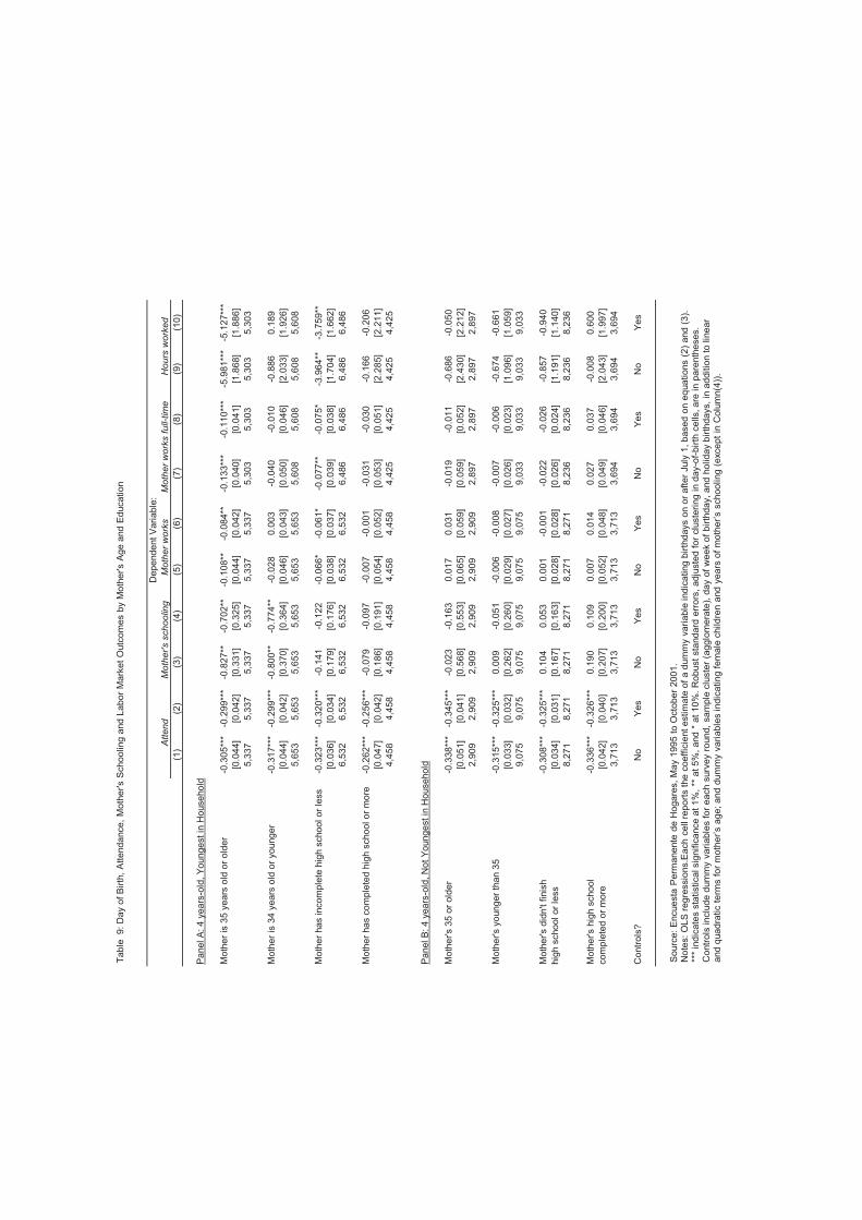
(1)

(2)

(3)

(4)

(5)

(6)

(7)

(8)

(9)

(10)

Panel A

: 4 y

ears

-old

, Y

oungest in

Household

Moth

er

is 3

5 y

ears

old

or

old

er

-0.3

05**

*-0

.299**

*-0

.827**

-0.7

02**

-0.1

08**

-0.0

84**

-0.1

33**

*-0

.110**

*-5

.981**

*-5

.127**

*

[0.0

44]

[0.0

42]

[0.3

31]

[0.3

25]

[0.0

44]

[0.0

42]

[0.0

40]

[0.0

41]

[1.8

68]

[1.8

86]

5,3

37

5,3

37

5,3

37

5,3

37

5,3

37

5,3

37

5,3

03

5,3

03

5,3

03

5,3

03

Moth

er

is 3

4 y

ears

old

or

younger

-0.3

17**

*-0

.299**

*-0

.800**

-0.7

74**

-0.0

28

0.0

03

-0.0

40

-0.0

10

-0.8

86

0.1

89

[0.0

44]

[0.0

42]

[0.3

70]

[0.3

64]

[0.0

46]

[0.0

43]

[0.0

50]

[0.0

46]

[2.0

33]

[1.9

26]

5,6

53

5,6

53

5,6

53

5,6

53

5,6

53

5,6

53

5,6

08

5,6

08

5,6

08

5,6

08

Moth

er

has incom

ple

te h

igh s

chool or

less

-0.3

23**

*-0

.320**

*-0

.141

-0.1

22

-0.0

66*

-0.0

61*

-0.0

77**

-0.0

75*

-3.9

64**

-3.7

59**

[0.0

36]

[0.0

34]

[0.1

79]

[0.1

76]

[0.0

38]

[0.0

37]

[0.0

39]

[0.0

38]

[1.7

04]

[1.6

62]

6,5

32

6,5

32

6,5

32

6,5

32

6,5

32

6,5

32

6,4

86

6,4

86

6,4

86

6,4

86

Moth

er

has c

om

ple

ted h

igh s

chool or

more

-0.2

62**

*-0

.256**

*-0

.079

-0.0

97

-0.0

07

-0.0

01

-0.0

31

-0.0

30

-0.1

66

-0.2

06

[0.0

47]

[0.0

42]

[0.1

86]

[0.1

91]

[0.0

54]

[0.0

52]

[0.0

53]

[0.0

51]

[2.2

85]

[2.2

11]

4,4

58

4,4

58

4,4

58

4,4

58

4,4

58

4,4

58

4,4

25

4,4

25

4,4

25

4,4

25

Dependent V

ari

able

:

Attend

Moth

er's s

choolin

gM

oth

er

work

sM

oth

er

work

s full-

tim

eH

ours

work

ed

Table

9: D

ay o

f B

irth

, A

ttendance,

Moth

er's S

chooling a

nd L

abor

Mark

et

Outc

om

es b

y M

oth

er's

Age a

nd E

ducation

4,4

58

4,4

58

4,4

58

4,4

58

4,4

58

4,4

58

4,4

25

4,4

25

4,4

25

4,4

25

Panel B

: 4 y

ears

-old

, N

ot Y

oungest in

Household

Moth

er's 3

5 o

r old

er

-0.3

38**

*-0

.345**

*-0

.023

-0.1

63

0.0

17

0.0

31

-0.0

19

-0.0

11

-0.6

86

-0.0

50

[0.0

51]

[0.0

41]

[0.5

68]

[0.5

53]

[0.0

65]

[0.0

59]

[0.0

59]

[0.0

52]

[2.4

30]

[2.2

12]

2,9

09

2,9

09

2,9

09

2,9

09

2,9

09

2,9

09

2,8

97

2,8

97

2,8

97

2,8

97

Moth

er's y

ounger

than 3

5-0

.315**

*-0

.325**

*0.0

09

-0.0

51

-0.0

06

-0.0

08

-0.0

07

-0.0

06

-0.6

74

-0.6

61

[0.0

33]

[0.0

32]

[0.2

62]

[0.2

60]

[0.0

29]

[0.0

27]

[0.0

26]

[0.0

23]

[1.0

96]

[1.0

59]

9,0

75

9,0

75

9,0

75

9,0

75

9,0

75

9,0

75

9,0

33

9,0

33

9,0

33

9,0

33

Moth

er's d

idn't

finis

h-0

.308**

*-0

.325**

*0.1

04

0.0

53

0.0

01

-0.0

01

-0.0

22

-0.0

26

-0.8

57

-0.9

40

hig

h s

chool or

less

[0.0

34]

[0.0

31]

[0.1

67]

[0.1

63]

[0.0

28]

[0.0

28]

[0.0

26]

[0.0

24]

[1.1

91]

[1.1

40]

8,2

71

8,2

71

8,2

71

8,2

71

8,2

71

8,2

71

8,2

36

8,2

36

8,2

36

8,2

36

Moth

er's h

igh s

chool

-0.3

36**

*-0

.326**

*0.1

90

0.1

09

0.0

07

0.0

14

0.0

27

0.0

37

-0.0

08

0.6

00

com

ple

ted o

r m

ore

[0.0

42]

[0.0

40]

[0.2

07]

[0.2

00]

[0.0

52]

[0.0

48]

[0.0

49]

[0.0

46]

[2.0

43]

[1.9

97]

3,7

13

3,7

13

3,7

13

3,7

13

3,7

13

3,7

13

3,6

94

3,6

94

3,6

94

3,6

94

Contr

ols

?N

oY

es

No

Yes

No

Yes

No

Yes

No

Yes

Sourc

e:

Encuesta

Perm

anente

de H

ogare

s,

May 1

995 t

o O

cto

ber

2001.

Note

s: O

LS

regre

ssio

ns.E

ach c

ell r

eport

s the c

oeffic

ient estim

ate

of

a d

um

my v

ari

able

indic

ating b

irth

days o

n o

r after

July

1, based o

n e

quations (

2)

and (

3).

**

* in

dic

ate

s s

tatistical sig

nific

ance a

t 1%

, **

at 5%

, and *

at 10%

. R

obust

sta

ndard

err

ors

, adju

ste

d for

clu

ste

ring in d

ay-o

f-bir

th c

ells, are

in p

are

nth

eses.

C

ontr

ols

inclu

de d

um

my v

ari

able

s for

each s

urv

ey r

ound,

sam

ple

clu

ste

r (a

gglo

mera

te),

day o

f w

eek o

f bir

thday, and h

oliday b

irth

days,

in a

dditio

n to lin

ear

and q

uadra

tic t

erm

s f

or

moth

er’

s a

ge; and d

um

my v

ari

able

s indic

ating fem

ale

childre

n a

nd y

ears

of m

oth

er’

s s

chooling (

except

in C

olu

mn(4

)).

(1)

(2)

(3)

(4)

(5)

(6)

(7)

(8)

(9)

(10

)

Pa

ne

l A

: Y

ou

ng

est

in H

ou

se

ho

ld

5 y

ea

r-o

lds

-0.0

20

-0.0

14

-0.8

87

***

-0.8

28

***

-0.0

56

*-0

.02

5-0

.08

2**

-0.0

47

-3.6

01

***

-2.4

55

*

[0.0

14

][0

.01

4]

[0.3

24

][0

.31

3]

[0.0

34

][0

.03

1]

[0.0

34

][0

.03

1]

[1.3

70

][1

.26

3]

10

,12

61

0,1

26

10

,12

61

0,1

26

10

,12

61

0,1

26

10

,05

21

0,0

52

10

,05

21

0,0

52

6 y

ea

r-o

lds

-0.0

05

-0.0

05

-0.5

02

-0.4

57

0.0

25

0.0

38

0.0

28

0.0

44

1.9

66

2.6

08

*

[0.0

04

][0

.00

4]

[0.3

18

][0

.32

2]

[0.0

33

][0

.03

1]

[0.0

37

][0

.03

5]

[1.4

26

][1

.34

7]

9,2

35

9,2

35

9,2

35

9,2

35

9,2

35

9,2

35

9,1

64

9,1

64

9,1

64

9,1

64

De

pe

nd

en

t V

ari

ab

le:

Mo

the

r w

ork

s f

ull-

tim

eH

ou

rs w

ork

ed

Att

en

dM

oth

er's s

ch

oo

ling

Mo

the

r w

ork

s

Ta

ble

10

: D

ay o

f B

irth

, A

tte

nd

an

ce

, M

oth

er's S

ch

oo

ling

an

d L

ab

or

Ma

rke

t O

utc

om

es a

t A

ge

s 5

an

d 6

Pa

ne

l B

: N

ot

Yo

un

ge

st

in H

ou

se

ho

ld

5 y

ea

r-o

lds

-0.0

17

-0.0

18

-0.0

51

-0.0

59

-0.0

05

0.0

01

-0.0

17

-0.0

16

-0.4

09

-0.2

84

[0.0

15

][0

.01

3]

[0.2

40

][0

.23

2]

[0.0

30

][0

.02

6]

[0.0

27

][0

.02

4]

[1.0

95

][1

.01

7]

13

,41

51

3,4

15

13

,41

51

3,4

15

13

,41

51

3,4

15

13

,33

61

3,3

36

13

,33

61

3,3

36

6 y

ea

r-o

lds

-0.0

01

-0.0

02

0.2

35

0.3

05

0.0

34

0.0

31

0.0

20

.01

70

.70

60

.64

5

[0.0

06

][0

.00

6]

[0.2

74

][0

.26

1]

[0.0

28

][0

.02

5]

[0.0

26

][0

.02

3]

[1.1

18

][1

.01

0]

14

,18

41

4,1

84

14

,18

41

4,1

84

14

,18

41

4,1

84

14

,09

61

4,0

96

14

,09

61

4,0

96

Co

ntr

ols

?N

oY

es

No

Ye

sN

oY

es

No

Ye

sN

oY

es

So

urc

e: E

ncu

esta

Pe

rma

ne

nte

de

Ho

ga

res,

Ma

y 1

99

5 t

o O

cto

be

r 2

00

1.

No

tes: O

LS

reg

ressio

ns. E

ach

ce

llre

po

rts t

he

co

eff

icie

nt e

stim

ate

of

a d

um

my v

ari

ab

le in

dic

atin

g b

irth

da

ys o

n o

r a

fte

r Ju

ly 1

, b

ase

d o

n e

qu

atio

ns (

2)

an

d (

3).

**

* in

dic

ate

s s

tatistica

l sig

nific

an

ce

at

1%

, **

at

5%

, a

nd

* a

t 1

0%

. R

ob

ust

sta

nd

ard

err

ors

, a

dju

ste

d

for

clu

ste

rin

g in

da

y-o

f-b

irth

ce

lls, a

re in

pa

ren

the

se

s.

Co

ntr

ols

in

clu

de

du

mm

y v

ari

ab

les f

or

ea

ch

su

rve

y r

ou

nd

, sa

mp

le c

luste

r (a

gg

lom

era

te),

da

y o

f w

ee

k o

f b

irth

da

y,

an

d h

olid

ay b

irth

da

ys,

in a

dd

itio

n to

lin

ea

r a

nd

qu

ad

ratic t

erm

s o

f fo

r m

oth

er’

s a

ge

;a

nd

d

um

my v

ari

ab

les in

dic

atin

g f

em

ale

ch

ildre

n a

nd

ye

ars

of

mo

the

r’s s

ch

oo

ling

(e

xce

pt

in C

olu

mn

(4

)).

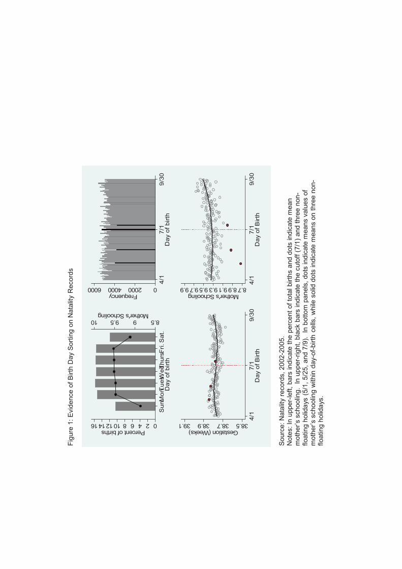
Fig

ure

1:

Evid

ence o

f B

irth

Day S

ort

ing o

n N

ata

lity R

ecord

s

8.599.510Mother's Schooling

0246810121416Percent of births

Sun.M

on.Tu

es.W

ed.

Thurs

.Fri.S

at.

Day o

f birth

0200040006000Frequency

4/1

7/1

9/3

0D

ay o

f birth

39.1

9.9S

ourc

e: N

ata

lity r

ecord

s, 2002-2

005.

Note

s: In

upper-

left

, bars

indic

ate

the p

erc

ent

of to

tal birth

s a

nd d

ots

indic

ate

mean

moth

er’s s

choolin

g.

In u

pper-

right, b

lack b

ars

indic

ate

the c

uto

ff (

7/1

) and t

hre

e n

on-

floating h

olid

ays (

5/1

, 5/2

5,

and 7

/9).

In

bottom

panels

, dots

indic

ate

means v

alu

es o

f m

oth

er’s s

choolin

g w

ithin

day-o

f-birth

cells

, w

hile

solid

dots

indic

ate

means o

n t

hre

e n

on-

floating h

olid

ays.

38.538.738.939.1Gestation (Weeks)

4/1

7/1

9/3

0D

ay o

f B

irth

8.78.99.19.39.59.79.9Mother's Schooling

4/1

7/1

9/3

0D

ay o

f B

irth

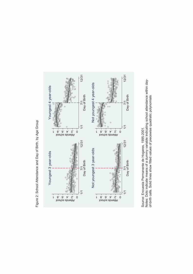
Fig

ure

2:

School A

ttendance a

nd D

ay o

f B

irth

, by A

ge G

roup

0.2.4.6.81Attends school

1/1

7/1

12/3

1D

ay o

f B

irth

Yo

un

ge

st 3

ye

ar-

old

s

0.2.4.6.81Attends school

1/1

7/1

12/3

1D

ay o

f B

irth

Yo

un

ge

st 4

ye

ar-

old

s

Sourc

e: E

ncuesta

Perm

anente

de H

ogare

s,

1995-2

001.

Note

s: D

ots

indic

ate

means o

f a d

um

my v

ariable

indic

ating s

chool attendance w

ithin

day-

of-

birth

cells

. S

olid

lin

es s

how

fitte

d v

alu

es o

f pie

cew

ise q

uadra

tic p

oly

nom

ials

0.2.4.6.81Attends school

1/1

7/1

12/3

1D

ay o

f B

irth

No

t yo

un

gest 3

ye

ar-

old

s

0.2.4.6.81Attends school

1/1

7/1

12/3

1D

ay o

f B

irth

No

t yo

un

gest 4

ye

ar-

old

s

Fig

ure

3:

Moth

er's S

choolin

g a

nd D

ay o

f B

irth

, by A

ge G

roup

7891011Mother's schooling

1/1

7/1

12/3

1D

ay o

f B

irth

Yo

un

ge

st 3

ye

ar-

old

s

7891011Mother's schooling

1/1

7/1

12/3

1D

ay o

f B

irth

Yo

un

ge

st 4

ye

ar-

old

s

Sourc

e: E

ncuesta

Perm

anente

de H

ogare

s,

1995-2

001.

Note

s: D

ots

indic

ate

means o

f a v

ariable

indic

ating y

ears

of

schoolin

g w

ithin

day-o

f-birth

cells

. S

olid

lin

es s

how

fitte

d v

alu

es o

f pie

cew

ise q

uadra

tic p

oly

nom

ials

7891011Mother's schooling

1/1

7/1

12/3

1D

ay o

f B

irth

No

t yo

un

gest 3

ye

ar-

old

s

7891011Mother's schooling

1/1

7/1

12/3

1D

ay o

f B

irth

No

t yo

un

gest 4

ye

ar-

old

s

Fig

ure

4:

Mate

rnal Labor

Outc

om

es a

nd C

hild

's D

ay o

f B

irth

, by A

ge G

roup

.1.2.3.4.5.6.7.8

Mother works

1/1

7/1

12/3

1D

ay o

f B

irth

You

ng

est

4 y

ear-

old

s

.1.2.3.4.5.6

Mother works full time

1/1

7/1

12/3

1D

ay o

f B

irth

You

ng

est

4 y

ear-

old

s

51015202530

Hours of work

1/1

7/1

12/3

1D

ay o

f B

irth

You

ng

est

4 y

ear-

old

s

Sourc

e: E

ncuesta

Perm

anente

de H

ogare

s,

1995-2

001.

Note

s: D

ots

indic

ate

means o

f a d

um

my v

ariable

s indic

ating e

mplo

ym

ents

, fu

ll-tim

e

em

plo

ym

ent

and

weekly

hours

of w

ork

, re

spectively

. S

olid

lin

es s

how

fitte

d v

alu

es o

f pie

cew

ise q

uadra

tic p

oly

nom

ials

.1.2.3.4.5.6.7.8Mother works

1/1

7/1

12/3

1D

ay o

f B

irth

No

t yo

un

ge

st

4 y

ea

r-o

lds

.1.2.3.4.5.6Mother works full time

1/1

7/1

12/3

1D

ay o

f B

irth

No

t yo

un

ge

st

4 y

ea

r-o

lds

51015202530Hours of work

1/1

7/1

12/3

1D

ay o

f B

irth

No

t yo

un

ge

st

4 y

ea

r-o

lds