Embed Size (px)
Citation preview

PRESCHOOL TELEVISION VIEWING AND ADOLESCENT TEST SCORES
HISTORICAL EVIDENCE FROM THE COLEMAN STUDY�
Matthew Gentzkow Jesse M. Shapiro
May 2007
Abstract
We use heterogeneity in the timing of television�s introduction to di¤erent local markets toidentify the e¤ect of preschool television exposure on standardized test scores during adolescence.Our preferred point estimate indicates that an additional year of preschool television exposureraises average adolescent test scores by about .02 standard deviations. We are able to rejectnegative e¤ects larger than about .03 standard deviations per year of television exposure. Forreading and general knowledge scores, the positive e¤ects we �nd are marginally statisticallysigni�cant, and these e¤ects are largest for children from households where English is not theprimary language, for children whose mothers have less than a high school education, and fornon-white children.
JEL classi�cation: I21, J13, J24
Keywords: television, cognitive ability, media
�We are grateful to Dominic Brewer, John Collins, Ronald Ehrenberg, Eric Hanushek, and Mary Morris (at ICPSR)for assistance with Coleman study data, and to Christopher Berry for supplying data on school quality. Lisa Furcht-gott, Jennifer Paniza, and Mike Sinkinson provided outstanding research assistance. We thank Marianne Bertrand,Stefano DellaVigna, Ed Glaeser, Austan Goolsbee, Jim Heckman, Caroline Hoxby, Larry Katz, Steve Levitt, EthanLieber, Jens Ludwig, Kevin M. Murphy, Emily Oster, Matthew Rabin, Andrei Shleifer, Chad Syverson, Bob Topel,and workshop participants at the University of Chicago, Harvard University, UC Berkeley, the NBER, the Universityof Notre Dame, and the APPAM for helpful comments. E-mail: [email protected], [email protected].
1

I Introduction
Television has attracted young viewers since broadcasting began in the 1940s. Concerns about
its e¤ects on the cognitive development of young children emerged almost immediately, and have
been fueled by academic research showing a negative association between early-childhood televi-
sion viewing and later academic achievement.1 These �ndings have contributed to a belief among
the vast majority of pediatricians that television has �negative e¤ects on brain development� of
children below age 5 [Gentile et al. 2004]. They have also provided partial motivation for recent
recommendations that preschool children�s television viewing time be severely restricted [American
Academy of Pediatrics 2001]. According to a widely-cited report on media use by young children,
�Many experts have argued that it is especially critical to understand media use by the youngest
children... because social and intellectual development are more malleable in these early years�
[Rideout, Vandewater, and Wartella 2003]. This view is supported by randomized studies demon-
strating large long-run e¤ects of preschool interventions on children�s cognitive skills [Currie 2001;
Schweinhart et al. 2005; Campbell and Ramey 1995].
Evidence of negative cognitive e¤ects has made the growth of television a popular explanation
for trends such as the decline in average verbal SAT scores during the 1970s [Wirtz et al. 1977; Winn
2002] and the secular decline in verbal ability across cohorts [Glenn 1994]. Given the important role
that cognitive skills play in individual [Griliches and Mason 1972] and aggregate [Bishop 1989] labor
market performance, understanding the cognitive e¤ects of television viewing may have signi�cant
implications for public policy and household behavior.
In this paper, we identify the e¤ect of preschool exposure to television on adolescent cognitive
skills by exploiting variation in the timing of television�s introduction to U.S. cities.2 Most cities �rst
received television between the early 1940s and the mid-1950s. The exact timing was a¤ected by
a number of exogenous events, most notably a four-year freeze on licensing prompted by problems
with the allocation of broadcast spectrum across cities. Once it was introduced, television was
adopted rapidly by families with children. Survey evidence suggests that young children who had
television in their homes during this period watched as much as three and a half hours per day, and
contemporary time-use studies show reductions in a wide range of alternative activities, including
sleep, homework, and outdoor play. Evidence on television ownership suggests that the di¤usion
2

of television was broad-based, reaching families in many di¤erent socioeconomic strata. Together,
these facts create a promising laboratory in which to study the e¤ects of television on children.
To conduct our analysis, we use data from a 1965 survey of American schools and school
children commonly referred to as the Coleman Study. The data include standardized test scores of
over 300,000 students who were in grades 6, 9, and 12 in 1965. These students were born between
1948 and 1954, just as television was expanding throughout the United States. Since television
entered di¤erent U.S. markets at di¤erent times, students were exposed to varying amounts of
television as preschoolers. Students in our sample range from those who had television in their local
area throughout their lives (for example, sixth graders whose areas got television between 1945 and
1954) to those whose areas only began receiving broadcasts after they reached age 6 (twelfth graders
whose areas got television in 1954). Because the Coleman sample includes students of di¤erent ages
within the same television market, we can identify the e¤ects of television by comparing test scores
across cohorts within a given area. This di¤erences-in-di¤erences approach allows us to estimate
the e¤ect of preschool television exposure on adolescent test scores, while holding constant �xed
characteristics of a locale that a¤ect test scores and might also be correlated with the timing of
television introduction.
We �nd strong evidence against the view that childhood television viewing harms the cogni-
tive or educational development of preschoolers. Our preferred point estimate indicates that an
additional year of preschool television exposure raises average adolescent test scores by about .02
standard deviations. We are able to reject negative e¤ects larger than about .03 standard devia-
tions per year of television exposure.3 For reading and general knowledge scores� domains where
intuition and existing evidence suggest that learning from television could be important� the pos-
itive e¤ects we �nd are marginally statistically signi�cant. In addition, we present evidence on
the extent to which childhood vieweing a¤ects later non-cognitive outcomes such as time spent on
homework and desired school completion, again �nding no consistent evidence of negative e¤ects.
A number of speci�cation checks support the identifying assumption that the timing of tele-
vision�s entry is uncorrelated with direct determinants of test scores. Most importantly, we �nd
that the within-area, cross-cohort variation in television exposure that identi�es our models does
not correlate with demographic variables that a¤ect test scores. We also �nd that the timing of
3
television introduction is uncorrelated with trends in area school quality, teacher characteristics,
and demographics. Thus, although by de�nition we cannot test that our key exposure measures are
orthogonal to unobservable variation in student ability, we show that these measures are unrelated
to many observable correlates of ability.
Our �nal set of results addresses heterogeneity in the e¤ects of television on test scores. The
e¤ects on verbal, reading, and general knowledge scores are most positive for children from house-
holds where English is not the primary language, for children whose mothers have less than a high
school education, and for non-white children. When we combine student observables into a single
index of parental investment� the time parents spent reading to their children in early childhood�
we �nd that the e¤ect of television is signi�cantly more positive the lower is parental investment.
Consistent with a rational-choice model, families in which television has relatively positive e¤ects
on learning also allocate more time to viewing.4
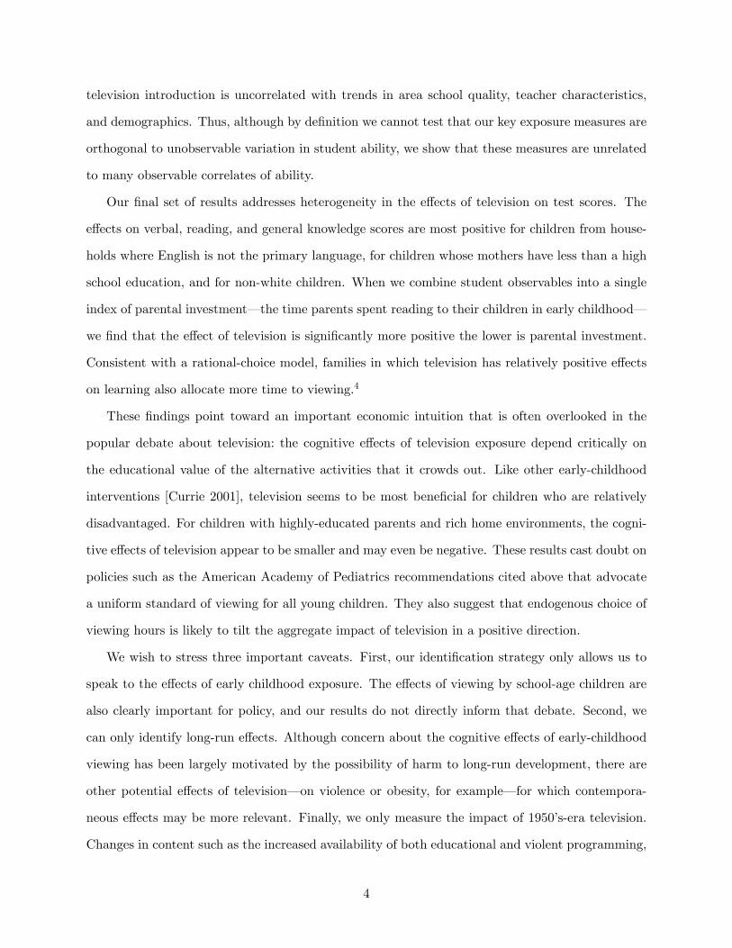
These �ndings point toward an important economic intuition that is often overlooked in the
popular debate about television: the cognitive e¤ects of television exposure depend critically on
the educational value of the alternative activities that it crowds out. Like other early-childhood
interventions [Currie 2001], television seems to be most bene�cial for children who are relatively
disadvantaged. For children with highly-educated parents and rich home environments, the cogni-
tive e¤ects of television appear to be smaller and may even be negative. These results cast doubt on
policies such as the American Academy of Pediatrics recommendations cited above that advocate
a uniform standard of viewing for all young children. They also suggest that endogenous choice of
viewing hours is likely to tilt the aggregate impact of television in a positive direction.
We wish to stress three important caveats. First, our identi�cation strategy only allows us to
speak to the e¤ects of early childhood exposure. The e¤ects of viewing by school-age children are
also clearly important for policy, and our results do not directly inform that debate. Second, we
can only identify long-run e¤ects. Although concern about the cognitive e¤ects of early-childhood
viewing has been largely motivated by the possibility of harm to long-run development, there are
other potential e¤ects of television� on violence or obesity, for example� for which contempora-
neous e¤ects may be more relevant. Finally, we only measure the impact of 1950�s-era television.
Changes in content such as the increased availability of both educational and violent programming,
4

as well as changes in the non-television alternatives available to young children, could mean that
the e¤ects of television viewing today are di¤erent from those we estimate.
Our study contributes to a large literature on the cognitive e¤ects of television, most of
which identi�es the e¤ect of television using cross-sectional variation in children�s viewing inten-
sity.5 It also contributes to a growing economic literature on the e¤ects of media on children
[Dahl and DellaVigna 2006], and on the e¤ects of mass media more generally (see, for example,
Djankov, McLiesh, Nenova and Shleifer 2003; Gentzkow and Shapiro 2004 and 2006; Gentzkow
2006; Stromberg 2004; DellaVigna and Kaplan, 2007; and Olken 2006).
The remainder of the paper is organized as follows. Section II discusses the history of the
introduction and di¤usion of television. Section III presents our data. Section IV discusses our
identi�cation strategy and reduced-form �ndings. Section V presents estimates of the e¤ect of
preschool television exposure on cognitive development and student achievement, and Section VI
presents an analysis of heterogeneity across students. Section VII concludes.
II The Introduction and Di¤usion of Television
The Federal Communications Commission (FCC) �rst licensed television for full-scale com-
mercial broadcasting on July 1, 1941.6 Two unexpected events intervened to delay television�s
expansion. The �rst was World War II: less than a year after the FCC authorization, the govern-
ment issued a ban on new television station construction to preserve materials for the war e¤ort.
Although some existing stations continued to broadcast, the total number of sets in use during
the war was less than 20,000. After the war, television expanded rapidly. Over 100 new licenses
were issued between 1946 and 1948, so that by 1950 half of the country�s population was reached
by television signals. This growth was again halted, however, by an FCC-imposed freeze on new
television licenses in September 1948. The FCC had determined that spectrum allocations did
not leave su¢ cient space between adjacent markets, causing excessive interference. The process of
redesigning the spectrum allocation took four years, and it was not until April 1952 that the freeze
was lifted and new licenses began to be issued.
The di¤usion of television ownership was rapid and demographically broad. Contemporaneous
polling data show that television penetration rose from 8 percent to 82 percent from 1949 to 1955
5

among those with high school degrees, and from 4 percent to 66 percent among those without.
Other demographic groups tend to show a similar pattern: television di¤usion was rapid among
both whites and non-whites, and among both elderly and non-elderly Americans.7 In households
with television, viewership had already surpassed four and a half hours per day by 1950 [Television
Bureau of Advertising 2003].
Children were among the most enthusiastic early viewers of television. Programs targeted
speci�cally at children were introduced early, with Howdy Doody making its debut in 1947 and a
number of popular series like Kukla, Fran, and Ollie, Jamboree Room, and Children�s Matinee on
the air by 1948 [Television January 1948]. Children�s programs accounted for more time on network
television than any other category in 1950 [Roslow 1952], and by 1951 advertisers were spending
$400,000 per week to reach the children�s market [Television August 1951]. Furthermore, children
were frequent viewers of programming primarily targeted at adults� to take one example, I Love
Lucy was ranked the most favored program among elementary-school students in 1952, 1953, and
1954 surveys [Television April 1955].8
There were no large-scale studies of children�s viewing hours in the 1950s, but a series of small
surveys make clear that intense viewing was common from television�s earliest years. Median daily
viewership in samples of elementary-school children ranged from 2.0 hours per day to 3.7 hours per
day, with the earliest studies showing 3.1 hours per day in 1948 (ages 6-12), 3.7 hours per day in
1950-51 (grades 6-7), 2.7 hours per day in 1951 (elementary ages), 3.3 hours in 1953 (elementary
ages), 3.7 hours in 1954 (grades 4-8), and 3.4 hours in 1955 (elementary ages).9 The only evidence
we are aware of on preschool viewing� a small survey of families in San Francisco in 1958� found
that weekday viewing averaged 0.7 hours per day for 3-year-olds, 1.6 hours per day for 4-year-olds,
and 2.3 hours per day for 5-year-olds, with weekend viewing on average half an hour to an hour
higher [Schramm, Lyle, and Parker 1961].
Two studies from the period document the dramatic changes that television brought to children�s
allocation of time. First, Maccoby [1951] surveyed 622 children in Boston in 1950 and 1951 and
matched children with and without television by age, sex, and socioeconomic status. The study
found that radio listening, movie watching, and reading were substantially lower in the television
group, but also that total media time was greater by approximately an hour and a half per day.10
6

The television group went to bed almost half an hour later, and spent less time on homework and
active play. The second study, conducted in 1959, surveyed children in two similar towns in Western
Canada of which only one had television available [Schramm, Lyle, and Parker 1961]. First-grade
children in the town with television watched for an average of an hour and 40 minutes per day.
They spent 35 fewer minutes listening to radio, 33 fewer minutes at play, 13 fewer minutes sleeping,
and 20 fewer minutes reading and watching movies. Sixth-grade children showed similar shifts in
time allocation and also spent 15 fewer minutes on homework.
III Measuring Test Scores and Television Exposure
III.A Test Scores in Grades 6-12
Our data on test scores will come from the the Coleman Study, formally titled Equality of
Educational Opportunity [Coleman 1966].11 The study includes data on 567,148 students who
were in grades 1, 3, 6, 9, or 12 in 1965. Sampling was conducted through the construction of
primary sampling units (PSUs) consisting of either counties or metropolitan areas. Because racial
di¤erences were a primary focus of the study, PSUs, school districts, and schools were selected so
that non-white students were oversampled relative to the U.S. population.
Within sample schools, all students were included in the study. Each student completed a
survey and an exam, both of which were administered in the fall of 1965. We will focus our analysis
on sixth, ninth, and twelfth graders because these students�birth cohorts (1948-1954) span most
of the period during which television was introduced, and because exam style and format were
fairly similar across these di¤erent grades. Exams for sixth, ninth and twelfth graders contained
sections on mathematics, spatial reasoning, verbal ability (vocabulary), and reading; ninth and
twelfth graders completed an additional section on general knowledge. In addition to information
on test scores, we extracted data on demographic characteristics from the student surveys. We
tried to include all characteristics that were available and reasonably comparable across all three
grades.
To select sample schools, the surveyors �rst chose schools with twelfth grades. Then, for each
school containing a twelfth grade, they identi�ed the middle and elementary schools that �fed�
their students into the secondary school. If a lower-grade school fed more than 90 percent of its
7

students into the selected twelfth-grade school, then it was sampled with certainty; other lower-
grade schools were sampled in proportion to the share of their students who were fed into the
twelfth-grade school. The Coleman data contain a school identi�er variable unique to each sampled
school containing a twelfth grade. For students in lower-grade schools, this identi�er refers to the
sampled twelfth-grade school into which the students were fed. We will employ this identi�er to
estimate speci�cations with �school��xed e¤ects, though we note that in the case of sixth graders
attending schools without a twelfth grade, it may be better thought of as a school district �xed
e¤ect.
For schools located in metropolitan areas, our data match the school identi�er to the Standard
Metropolitan Statistical Area (SMSA) in which the school was located in 1965. For all other
schools, the data identify the county in which the school was located.12 To estimate the extent to
which students in the Coleman sample were exposed to television during early childhood, we will
assume that the television market where a student currently attends school is the same as the one
where he or she grew up. In section V.C below, we use direct data on students�mobility since early
childhood to show that this assignment is likely to be accurate for the vast majority of students,
and that our conclusions are, if anything, strengthened by excluding those who are most likely to
have grown up in a di¤erent market.
III.B Television Availability in Local Markets
Our estimation strategy relies on information about the availability of television in U.S. cities
beginning in 1946. We use data from Gentzkow [2006] on the year in which the �rst television station
appeared in a given market.13 These data were compiled from annual editions of the Television
Factbook. We de�ne television markets using the Designated Market Area (DMA) concept designed
by Nielsen Media Research (NMR). NMR assigns every county in the US to a television market
such that all counties in a given market have a majority of their measured viewing hours on stations
broadcasting from that market.14 We de�ne the year television was introduced to a given county
or SMSA to be the �rst year in which a station in its DMA broadcast for at least four months.
For the purposes of estimation, we will divide DMAs into three groups according to the year
in which they began receiving television broadcasts: early adopters (broadcasts begin in 1947 or
earlier), middle adopters (1948 to 1952), and late adopters (1953 or later). These categories, which
8

correspond to the period before, during, and after the FCC freeze, capture most of the relevant
variation in the data.
To illustrate the impact of broadcast availability on television ownership, we compare our avail-
ability measure with data on television ownership from the 1950 and 1960 U.S. Censuses. Figure
I shows the share of households owning televisions as a function of the year in which television
broadcasts began in the DMA. The �rst graph, which shows penetration in 1950, reveals a clear
distinction between counties that had a station in their DMA and those that did not. The average
penetration in DMAs whose �rst station began broadcasting before 1950 ranges from 8 percent in
the 1949 group to over 35 percent in the 1941 group, while the average for groups getting television
after 1950 never exceeds 1 percent. The second graph shows that, by 1960, di¤erences in pene-
tration across these DMAs had largely disappeared. Di¤erences in the timing of introduction of
television to di¤erent areas thus had a large initial impact, but by 1960 most late-adopting DMAs
had caught up to those that began receiving broadcasts early. These patterns will be crucial to
allowing us to identify the e¤ect of television using di¤erences across birth cohorts within a DMA.
An examination of historical records suggests two potential sources of endogeneity in the timing
of television�s introduction to a market. First, the FCC sought to maximize the number of people
who could receive a commercial television signal. Conditional on the quality of existing coverage in a
market, the FCC therefore handled applications to begin broadcasting in order of the market�s total
population [Television Digest 1953]. Second, since a station�s pro�tability was determined largely
by advertising revenue, which in turn depends on the spending power of the market�s population,
commercial interest in operating stations in a given market was highly related to the market�s total
retail sales or income.
The data con�rm the expected role of population and income. Early- and middle-adopting
DMAs had, on average, 5 times larger populations and 23 percent larger per capita incomes than
late-adopting DMAs. After controlling for log population and income, however, di¤erences between
early and late adopters appear much more idiosyncratic. Indeed, in regressions controlling for log
population and income, F -tests show no statistically signi�cant relationship between television
adoption category and percent high school educated, median age, and percent non-white at the
DMA level. (See the online appendix to this paper for details.) All of the models we estimate
9
below will control for DMA-level log population and income, so the parameters will be driven
solely by variation in the availability of television orthogonal to these two factors.15 In section
V.C below, we show formally that the remaining variation in television adoption timing is not
systematically related to student-level observables.
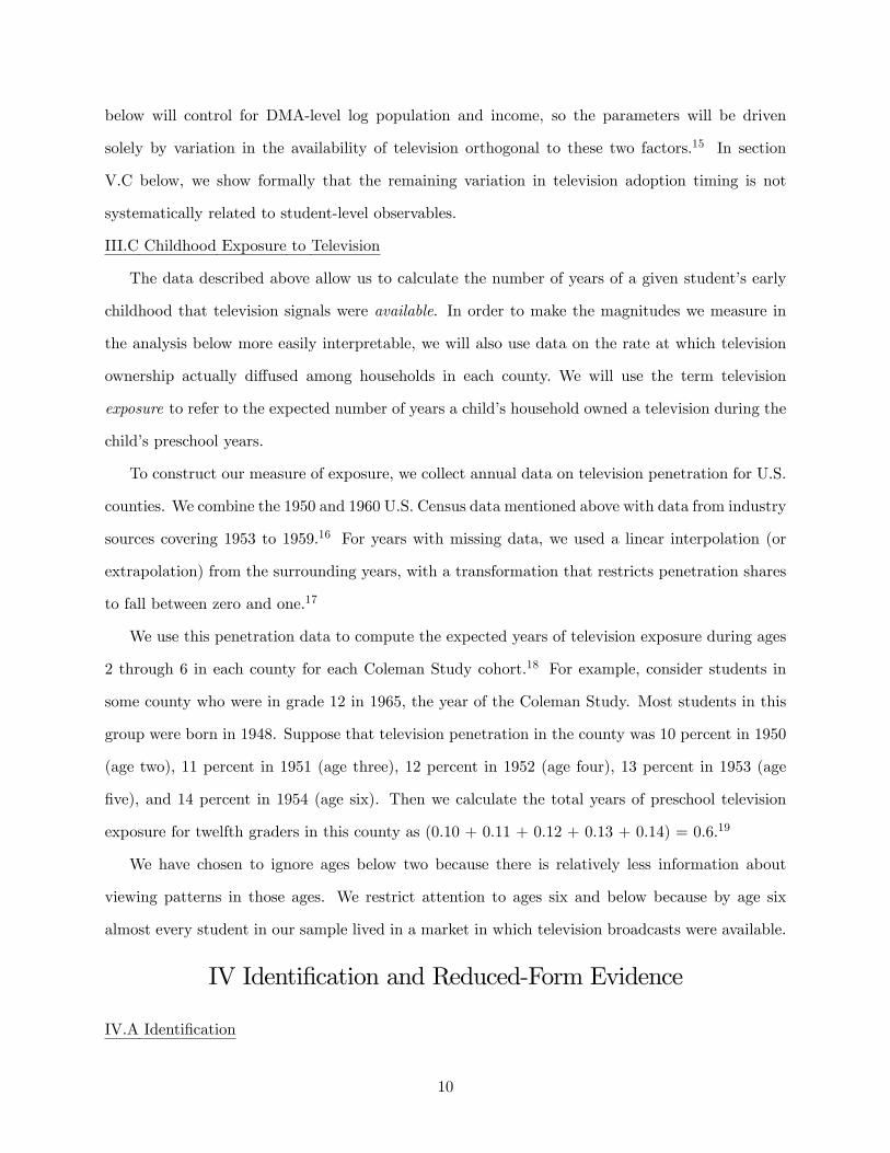
III.C Childhood Exposure to Television
The data described above allow us to calculate the number of years of a given student�s early
childhood that television signals were available. In order to make the magnitudes we measure in
the analysis below more easily interpretable, we will also use data on the rate at which television
ownership actually di¤used among households in each county. We will use the term television
exposure to refer to the expected number of years a child�s household owned a television during the
child�s preschool years.
To construct our measure of exposure, we collect annual data on television penetration for U.S.
counties. We combine the 1950 and 1960 U.S. Census data mentioned above with data from industry
sources covering 1953 to 1959.16 For years with missing data, we used a linear interpolation (or
extrapolation) from the surrounding years, with a transformation that restricts penetration shares
to fall between zero and one.17
We use this penetration data to compute the expected years of television exposure during ages
2 through 6 in each county for each Coleman Study cohort.18 For example, consider students in
some county who were in grade 12 in 1965, the year of the Coleman Study. Most students in this
group were born in 1948. Suppose that television penetration in the county was 10 percent in 1950
(age two), 11 percent in 1951 (age three), 12 percent in 1952 (age four), 13 percent in 1953 (age
�ve), and 14 percent in 1954 (age six). Then we calculate the total years of preschool television
exposure for twelfth graders in this county as (0.10 + 0.11 + 0.12 + 0.13 + 0.14) = 0.6.19
We have chosen to ignore ages below two because there is relatively less information about
viewing patterns in those ages. We restrict attention to ages six and below because by age six
almost every student in our sample lived in a market in which television broadcasts were available.
IV Identi�cation and Reduced-Form Evidence
IV.A Identi�cation
10

The key advance of this study relative to previous work is to identify the e¤ect of television
on test scores using variation across local markets in the timing of television�s introduction. In
appendix I, we use the Coleman data to examine the potential biases in an approach that uses
cross-sectional correlations between television viewing and test scores, as is done in the bulk of
the existing literature. We show that virtually every observable characteristic in our data that is
related to test scores is also strongly correlated with television viewing hours. Depending on which
set of characteristics we include as controls, we can reproduce highly signi�cant partial correlations
of television and test scores that are either positive or negative. This suggests that inferring causal
relationships from such correlations is a dubious enterprise.
To illustrate our approach to identi�cation, suppose that childhood television viewing has a
negative e¤ect on test scores. Consider two cities, an early adopter where television was introduced
in 1948, and a late adopter where it was introduced in 1954. In the �rst city, sixth, ninth, and
twelfth graders were all able to watch television throughout childhood (recall that twelfth graders
in the Coleman Study were born in 1948). In the second city, sixth graders had television available
throughout their lives, but ninth graders only had access to it starting at age three and twelfth
graders only at age six. We would therefore expect twelfth graders in the second city to perform
well relative to sixth and ninth graders in that city, and ninth graders to perform slightly better
than sixth graders. In the �rst city, we would expect no such pattern. By di¤erencing out the
mean test scores by grade from the �rst city, we could isolate the e¤ects of television using grade
patterns in the second city.
A simple way to implement this strategy would be to run a regression of test scores on the
number of preschool years that television broadcasts were available in a student�s city, controlling
for grade and city �xed e¤ects. Cities where television availability did not vary across grades
would identify the grade �xed e¤ects; sixth graders, for whom television was available throughout
childhood in essentially all cities, would identify the city �xed e¤ects. The remaining variation in
the grade pattern of test scores between cities would identify the parameter on years of availability.
Note that the interpretation of these results� denominated in years of television broadcast
availability rather than years a child actually had a television in her home� would di¤er greatly
depending on the speed at which television ownership di¤used. A given e¤ect of a year of television
11

availability could re�ect a large e¤ect of exposure if few households actually adopted, or a much
smaller e¤ect if adoption was widespread.
In order to make the magnitudes of our coe¢ cients more directly interpretable, we therefore wish
to scale our estimates using data on television exposure, constructed as described in the previous
section. One way to do this would be to simply replace availability with exposure on the right-hand
side. But these results would be identi�ed in part by variation in television purchase decisions�
likely to be strongly correlated with county-level unobservables� rather than by variation in the
timing of television�s introduction. Instead, we adopt a two-stage least squares (2SLS) approach.
We include exposure on the right-hand side, but instrument for it using data on the year in which
television was �rst introduced. This means that the model will be identi�ed solely by variation in
the timing of television�s introduction, but the magnitudes will be interpretable as the e¤ect of a
year of actual television exposure.20
To state this approach more formally, let ygc be the average test scores of students in grade g in
location c, measured as of 1965. Given the geographic information included in the Coleman data,
we will de�ne a location to be either an SMSA or a county (for areas not in SMSAs). Let TVgc be
the number of years of preschool television exposure of the average student in grade g and location
c, constructed as described in section III.C above. We can write
(1) ygc = �TVgc + �gWc + �c + g + "gc
where �c and g are location and grade �xed e¤ects, respectively, and "gc is a city-grade level error
term, possibly correlated across grades within a city.21
The term �gWc represents the DMA-level log population and log income of a location Wc
multiplied by a grade-speci�c coe¢ cient vector �g, where the population and income �gures are
taken from the 1960 Census. As discussed above, an examination of the historical record suggests
that DMA population and income were the most important observable predictors of the timing
of television�s introduction. Although our identi�cation strategy will rely only on changes across
cohorts within a given market (rather than di¤erences across markets), including income and pop-
ulation controls (interacted with grade) will limit the chance that our results will be confounded
12

by unobserved di¤erences in cohort or time trends across markets of di¤erent size or wealth.22
We instrument for TVgc with interactions between grade dummies and dummies for whether
the city was an early, middle, or late adopter of television. The �rst stage of this model can be
written as
(2) TVgc = �0gADOPTc + �
0gWc + �
0c +
0g + "
0gc
where ADOPTc is a vector of dummies indicating whether location c was an early, middle, or late
adopter of television and �0g is a separate vector of parameters for each grade g. The instruments
�0gADOPTc capture the critical cross-city-cross-grade variation in the availability of television that
will identify the e¤ect of exposure. The crucial identifying assumption in this model is that,
conditional on the controls, the interaction between the timing of television introduction and the
birth cohort of the student is orthogonal to the error term in equation (1). Under this assumption,
our estimate of the parameter � in equation 1 will be interpretable as the causal e¤ect of an
additional year of preschool television exposure on test scores.
Although our model can be estimated with aggregate data alone, we wish to take advantage of
the availability of the individual-level data in the Coleman sample. This will allow us to include
tighter controls for geography, in particular permitting the use of school, rather than location �xed
e¤ects. It will also allow us to control for characteristics of individual households and students that
might a¤ect exam performance. Both types of information would be expected to improve precision.
Of course, because the timing of television introduction is measured at the DMA level, in moving to
microdata we must be careful to avoid aggregation bias [Moulton 1990]. We will therefore cluster
our standard errors at the DMA level, which will also account for any serial correlation across
di¤erent grades within the same DMA [Bertrand, Du�o and Mullainathan 2004].23
In the next subsection, we present OLS estimates of the �rst-stage equation (2) and of the
reduced-form second stage. In section V we present 2SLS estimates of equation (1). We note that
the latter estimates are necessarily local to the students whose exposure to television was a¤ected
by the introduction of television [Angrist 2004], so that students in households whose decision to
adopt television was more responsive to broadcast availability would implicitly receive more weight
13

in our estimation. In section VI, we provide evidence on the heterogeneity in treatment e¤ects in
the student population and discuss how this heterogeneity is related to television viewership rates.
IV.B First-stage and Reduced-form Estimates
Before estimating model (1) formally, it will be helpful to examine the variation that will identify
it. In �gure II, we plot the coe¢ cients from year-by-year regressions of DMA television penetration
on a dummy for having received a television station before 1953 (controlling for log population and
log income). The �gure thus shows how pre-1953 television introduction�s impact on penetration
changes over time. During the period from 1948 to 1954, when the twelfth graders in the Coleman
sample were of preschool age, television penetration was substantially higher in early- and middle-
adopting DMAs than in late-adopting DMAs. By contrast, in the post-1954 period, when the
sixth graders in the sample were preschoolers, the late adopters (most of which received television
by 1954) had largely caught up to the early- and middle-adopters. In other words, di¤erences in
adoption dates across DMAs had the largest impact on television exposure for the twelfth graders in
the sample, a smaller impact on the ninth graders, and only a minimal impact on the sixth graders.
This interaction between a student�s grade and the impact of the timing of television introduction
is what will allow us to estimate the e¤ect of television exposure on test scores.
Turning to formal estimation, column (1) of table I presents estimates of the �rst-stage of our
model, regressing TVgc on interactions between grade dummies and dummies for whether the city
was an early, middle, or late adopter of television. Observe �rst that, for a given grade, television
exposure was lower the later television was introduced to the student�s city. So, for example,
students in grade nine whose DMAs adopted late were exposed to television for about :8 years less
than ninth graders whose DMAs adopted early, and about :5 years less than those whose DMAs
were middle adopters. A similar pattern is present for students in grade 12.
Next, note that, holding constant the timing of television�s introduction to a market, twelfth
graders on average had less preschool television exposure (between the ages of 2 and 6) than ninth
graders, and much less than sixth graders (the omitted category). For example, twelfth graders in
late-adopting DMAs had television in their homes for about 1:1 years less than sixth graders in
these same DMAs, and about :3 years less than ninth graders. This is what we would expect, since
twelfth graders were born in 1948, ninth graders were born in 1951, and sixth graders were born
14

in 1954. So in cities receiving television after 1948, ninth graders were more likely than twelfth
graders to spend their preschool years in a city in which a television signal was available, and sixth
graders were almost certain to have grown up with a television in the household.
These �ndings complement the evidence in �gure I in showing that the timing of broadcast
availability had a substantial impact on television penetration and hence on students�exposure to
television as young children. Each of the grade-timing interaction terms is strongly individually
signi�cant, and the F-test presented in table I de�nitively rejects the null hypothesis that these
interactions have no impact on exposure.24
In column (2), we present a reduced-form second-stage estimate of the e¤ect of our instruments
on test scores. We use as our dependent variable the average of the student�s (standardized)
scores on the math, reading, verbal, and spatial reasoning tests. If television exposure exerted a
negative long-term e¤ect on cognitive skills, we would expect the coe¢ cients on the grade-timing
interactions in column (2) to move inversely with the coe¢ cients in column (1). In other words, we
would expect the students who had relatively less childhood television exposure to perform better
on standardized tests. As the column shows, however, we do not see such a pattern. Although
students from middle-adopting DMAs perform slightly better than those from late-adopting DMAs,
these students perform worse than those from early-adopting DMAs. Additionally, among students
from middle-adopting DMAs, twelfth graders perform worse than ninth graders and sixth graders,
despite having spent more time without television in their households.
An F-test of the null hypothesis that the grade-timing interactions had no e¤ect on test scores
fails to reject at conventional signi�cance levels. Adding demographic controls in columns (3) and
(4) improves the precision of our estimates by explaining a larger share of the variation in test
scores. These more precise estimates show even less evidence of a negative e¤ect of television.
In column (4), where our standard errors are lowest, we �nd small point estimates on nearly all
interaction terms, and the di¤erences among these coe¢ cients do not support the hypothesis of a
negative e¤ect of television on test scores.
Finally, in column (5), we present reduced-form second-stage estimates of the e¤ect of our
instruments on the number of hours of contemporaneous (1965) television viewing. The grade-
timing interactions are both individually and jointly insigni�cant. This con�rms that our estimates
15

will capture the e¤ect of lagged rather than contemporaneous exposure.
V Television and Cognitive Development
V.A Two-stage Least Squares (2SLS) Estimates
In table II, we present estimates of equation (1) computed using 2SLS. Coe¢ cients in these
models can be interpreted as the causal e¤ect of a year of preschool television exposure on test
scores.
We present results for the average test score as well as for each individual component score. For
each test, we present baseline estimates, estimates with demographic controls, and estimates with
demographics interacted with a student�s grade. Adding controls should improve the precision of
our estimates by leaving a smaller share of the overall variation in test scores unexplained.
The �rst column shows our estimates of the e¤ect of an additional year of television exposure on
the student�s average test score, expressed in units of standard deviations (by grade). In general, we
�nd small, statistically insigni�cant, and positive estimates, suggesting that, if anything, childhood
television exposure improves a student�s test scores. Adding controls tends to increase the point
estimates and, consistent with expectations, decrease the standard errors of these estimates. In the
�nal speci�cation with demographic controls interacted with grade dummies, we are able to reject
negative e¤ects of television larger than about 0:03 standard deviations per year of exposure.25
The remaining columns present the estimated e¤ect of television on test scores in each subject
separately. In no case do we see clear evidence for a negative e¤ect of television. Column (2) shows
that the e¤ects on mathematics and spatial reasoning range from slightly negative to slightly positive
and are in all cases statistically insigni�cant. With our largest set of controls, we �nd point estimates
of �0:018 and 0:003 standard deviations per year of television exposure for mathematics and spatial
reasoning respectively. Our point estimates on verbal and reading scores are always positive, with
the e¤ect on reading scores a marginally statistically signi�cant 0:06 standard deviations in the
�nal speci�cation (p = 0:065). This in turn means that we can rule out even very small negative
e¤ects� our con�dence interval in this speci�cation excludes a negative e¤ect on reading scores of
about 0:004 standard deviations. Finally, the preferred point estimate for the e¤ect on general
knowledge is a positive e¤ect of about 0:07 standard deviations per year of television exposure.
16

Although we are reluctant to draw �rm conclusions from the comparison of coe¢ cients across
test scores, we note that the pattern of relatively positive e¤ects on verbal, reading, and general
knowledge scores is consistent with a variety of existing evidence suggesting that children can learn
language-based skills from television. For example, Rice [1983] argues that the presentation of
verbal information on television is especially conducive to learning by young children. Rice and
Woodsmall [1988] present laboratory evidence that children aged three and �ve can learn unfamiliar
words from watching television. The e¤ect on general knowledge scores might also re�ect the fact
that television also exposes young children to a large number of facts, some of which might be
retained into adolescence.26
V.B Interpretation of Magnitudes
To provide a better sense of the magnitudes of our coe¢ cients and standard errors, we can con-
trast them with experimental �ndings in which children exposed to an intervention as preschoolers
are followed into adolescence. Perhaps the two best-known instances of such experiments are the
Perry Preschool Study and the Carolina Abecedarian Project [Schweinhart et al. 2005; Campbell
and Ramey 1995].27 Both studies focused on children from relatively poor families. The Perry
study enrolled an intervention group in a two-year, part-day preschool education program during
ages 3 and 4. The Abecedarian project enrolled children in a �ve-year, full-day day care program
through age 5. In both cases, children were randomly assigned to intervention and control con-
ditions, and both sets of children were followed into adolescence. In the Perry program, children
in the intervention group scored one- to two-thirds of a standard deviation higher on achievement
tests at age 14 (the average age of students in our Coleman sample), with an overall e¤ect of about
one-half of a standard deviation. In the Abecedarian program, e¤ect sizes on achievement at age
15 were on the order of one-third of a standard deviation. Norming these e¤ects for the di¤erences
in treatment duration between the studies, the Perry program had an impact on achievement of
approximately 0:25 standard deviations per year of intervention, and the Abecedarian program had
an impact of approximately 0:07 to 0:08 standard deviations per year.28 The long-term e¤ects of
these preschool interventions therefore tend to exceed e¤ects on the order of the low end of our
main con�dence interval (about 0:03 standard deviations per year of television).
V.C Speci�cation Checks
17

Are the instruments correlated with student characteristics?
The models presented above are valid under the assumption that our instruments� interactions
between the timing of television introduction and grade� are orthogonal to the error term. Of
course, it is by de�nition impossible to test this assumption. Some relevant information, however,
can be obtained by asking whether television exposure is correlated with trends in observable de-
mographic characteristics. Although the absence of such a correlation is not proof of the identifying
assumption, it does provide some con�dence that unobserved heterogeneity is unlikely to bias our
estimates of the e¤ect of television.
There are two related possibilities we wish to test for. The �rst is that, in 1965, cross-grade
di¤erences in the household characteristics of students within an area are correlated with the timing
of television�s introduction. The second is that demographic trends during the 1950s are correlated
with the timing of television�s introduction, resulting in a relationship between a student�s preschool
television exposure and the local circumstances during her upbringing.
To conduct a test for the �rst possibility, we use the �rst-stage model (2) to create a predicted
number of years of television exposure for each student. By regressing this predicted value on a
set of demographic characteristics, we can test whether the variation in television exposure that is
due to the timing of television introduction is correlated with cross-grade di¤erences in observable
student characteristics that might be expected to a¤ect test scores.
The results of this test are presented in table III. None of the demographics has a statistically
signi�cant correlation with predicted television exposure. Additionally, an F-test of the joint hy-
pothesis that none of the demographic characteristics is correlated with years of television exposure
fails to reject (p = 0:170). Thus we �nd no evidence of a correlation between the local availability
of television and observable characteristics, once we control for DMA-level population and income.
This is true despite the fact that, as table III also shows, these demographic characteristics are in
most cases strong predictors of test scores.29
To test for a bias from di¤erences in time trends in demographics, we have also tested for a
relationship between the timing of the introduction of television and changes in income, population
density, and adult schooling levels by DMA in the 1950s (see online appendix for details). We �nd
no statistically signi�cant relationship and no consistent direction of correlation, lending further
18
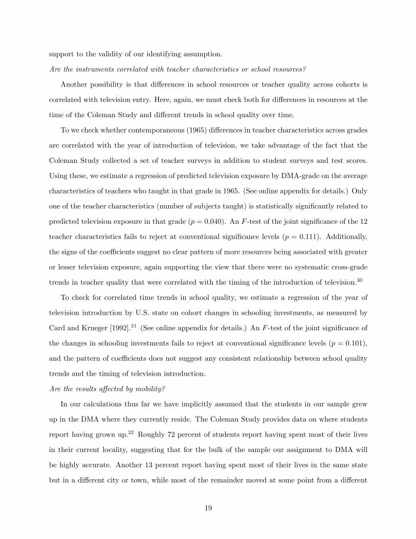
support to the validity of our identifying assumption.
Are the instruments correlated with teacher characteristics or school resources?
Another possibility is that di¤erences in school resources or teacher quality across cohorts is
correlated with television entry. Here, again, we must check both for di¤erences in resources at the
time of the Coleman Study and di¤erent trends in school quality over time.
To we check whether contemporaneous (1965) di¤erences in teacher characteristics across grades
are correlated with the year of introduction of television, we take advantage of the fact that the
Coleman Study collected a set of teacher surveys in addition to student surveys and test scores.
Using these, we estimate a regression of predicted television exposure by DMA-grade on the average
characteristics of teachers who taught in that grade in 1965. (See online appendix for details.) Only
one of the teacher characteristics (number of subjects taught) is statistically signi�cantly related to
predicted television exposure in that grade (p = 0:040). An F -test of the joint signi�cance of the 12
teacher characteristics fails to reject at conventional signi�cance levels (p = 0:111). Additionally,
the signs of the coe¢ cients suggest no clear pattern of more resources being associated with greater
or lesser television exposure, again supporting the view that there were no systematic cross-grade
trends in teacher quality that were correlated with the timing of the introduction of television.30
To check for correlated time trends in school quality, we estimate a regression of the year of
television introduction by U.S. state on cohort changes in schooling investments, as measured by
Card and Krueger [1992].31 (See online appendix for details.) An F -test of the joint signi�cance of
the changes in schooling investments fails to reject at conventional signi�cance levels (p = 0:101),
and the pattern of coe¢ cients does not suggest any consistent relationship between school quality
trends and the timing of television introduction.
Are the results a¤ected by mobility?
In our calculations thus far we have implicitly assumed that the students in our sample grew
up in the DMA where they currently reside. The Coleman Study provides data on where students
report having grown up.32 Roughly 72 percent of students report having spent most of their lives
in their current locality, suggesting that for the bulk of the sample our assignment to DMA will
be highly accurate. Another 13 percent report having spent most of their lives in the same state
but in a di¤erent city or town, while most of the remainder moved at some point from a di¤erent
19

state. Because DMAs often include a large fraction of a state�s population, many of the 13 percent
who moved from a di¤erent town will still be assigned correctly. The assignment of the remaining
students will be noisier, but since nearly half of DMAs (and thus television markets) spill across
state boundaries, a student�s current residence may still contain some information about his or her
childhood DMA.
We have estimated our main speci�cation separately for students who grew up in their current
state, and those who grew up outside of their current state. As expected, our coe¢ cients are
generally stronger (more positive) for those in the former group. (See online appendix for details.)
Does television exposure drive sample selection?
There are two possible sources of endogenous selection bias in our estimates. The �rst is
that preschool television exposure a¤ects the rate of high school completion, and thus a¤ects the
composition of students who appear in the twelfth grade portion of the Coleman sample. The
second is that television exposure a¤ects participation in the Coleman study conditional on being
enrolled in school, say because of e¤ects on attendance.
The evidence in table III (discussed above) speaks to both of these concerns. It shows that
observable correlates of test scores appear to be balanced with respect to preschool television
exposure. If television exposure changes the distribution of test scores conditional on selecting into
the Coleman sample, we would expect it to a¤ect the conditional distribution of other observable
characteristics as well. For example, if exposure causes more low-achieving students to drop out
of school between the ninth and twelfth grades, we would expect to see relatively fewer twelfth
graders with low test scores in high-exposure areas. However, we would expect to see relatively
fewer twelfth graders with low family income and parental education as well. The fact that we do
not see this pattern suggests that selection is unlikely to be biasing the results.
To more directly address the possibility that television exposure a¤ects dropout rates, we use
Census microdata to study the e¤ect of television exposure on high school completion (see online
appendix for details). There is no evidence that preschool television exposure a¤ects the likelihood
of having completed high school as of adulthood, although we note that the precision of these
estimates is lower than the precision of estimates based on the Coleman data.
We have also re-estimated our models excluding twelfth graders, who are most likely to have
20
selectively dropped out of school prior to surveying (results not shown). As expected, the standard
errors of our models increase due to the exclusion of a large portion of the data, but the resulting
regressions continue to show no evidence of negative e¤ects of television.
Finally, to investigate e¤ects of television on selection into the pool of Coleman test takers, we
have compared the number of students in the Coleman sample with the number we would predict
based on principals�reports of school sizes (in the spirit of Jencks, 1972). We �nd no evidence that
television exposure a¤ected rates of inclusion in the Coleman sample.
V.D Television and Non-cognitive Outcomes
The analysis above addresses the e¤ect of television viewing on cognitive development. But
it may be that many of television�s most important e¤ects are on non-cognitive traits.33 We
can use the Coleman data to estimate the e¤ect of early-childhood television exposure on several
social and behavioral outcomes in later years. We note that, as with the previous analysis, our
data do not permit us to say anything about the e¤ect of television on contemporaneous non-
cognitive outcomes. Table IV reports 2SLS estimates of the e¤ect of preschool television exposure
on several adolescent attitudinal and behavioral outcomes. The e¤ects are mostly small, negative,
and statistically insigni�cant. The main exception is a marginally statistically signi�cant negative
e¤ect on the number of books a student reads during the summer. We also �nd a statistically
insigni�cant and small positive e¤ect on the number of hours the student spends on homework
each day.
We have also used data from the Integrated Public Use Microdata Series [Ruggles et al. 2004]
to test for e¤ects of television on long-run labor market outcomes. We extracted information on
schooling attainment and wages for cohorts born in 1948, 1951, and 1954 from the 1970, 1980,
1990, and 2000 1% samples of the Census. Information on state of birth provides a coarse measure
of the geographic area in which individuals lived in early childhood, allowing us to apply a similar
identi�cation strategy to estimate the causal impact of television. The results show no evidence of
a negative e¤ect of television, although the coarseness of the geographic identi�ers means that the
precision of these estimates is limited. Details of this exercise are available in our online appendix.
VI Heterogeneity in the E¤ects of Television
21

Our results thus far focus on the e¤ect of preschool television exposure on the test scores of the
average student in our dataset. For many purposes, however, it will be important to know how the
e¤ects of television are distributed in the population, especially with respect to the socioeconomic
status of the student�s household. A body of evidence from developmental psychology shows that
the in-home learning environment is richer in higher-socioeconomic-status households, especially
with respect to language and vocabulary [Hart and Risley 1995 and 1999]. Embedded in a simple
time-allocation framework [Becker 1965], this evidence would lead one to expect that television is
more bene�cial to children from more disadvantaged backgrounds, because for such children the
activities crowded out by television are likely to be less cognitively stimulating.34 Of course, this
prediction could change if richer or more educated parents are better able to select educational
programming for their children to watch.35
In this section, we o¤er evidence on the question of which children bene�t the most (or are
harmed the least) from television exposure. On the whole, our �ndings support the prediction that
television is most bene�cial to children in households with the least parental human capital.
In table V, we present a �rst look at heterogeneous e¤ects by splitting the sample along several
salient demographic dimensions. The �rst two columns repeat our basic 2SLS speci�cation for
students whose mothers do and do not have a high school education.36 The estimated e¤ect of a
year of television exposure on the average test score is 0:04 for students whose mothers have less
than a high-school education, and 0:01 for students whose mothers have a high-school degree. A
similar pattern is present for individual test scores.
The next two columns compare households where English was and was not the primary language.
The estimated e¤ects of television on verbal, reading, and general knowledge scores for students
in non-English-speaking households are positive and nontrivial in magnitude. For the sample of
students whose family members primarily speak English, the point estimates are still positive, but
are much smaller. The point estimates for math and spatial reasoning also suggest more positive
e¤ects for students in non-English-speaking households.
In the �nal two columns, we present results for white and non-white students. We �nd that
non-white students bene�t considerably more from television exposure than do white students.
The point estimate of the e¤ect on average test scores is more than 0:05 for non-white students, as
22

compared to less than 0:01 for white students.
To combine the information from these various subsample comparisons, we take advantage of
a question in the Coleman Study survey that asks students how often they were read to at home
prior to starting school. The possible responses range from �never�to �regularly.�We anticipate
that this measure will be correlated with the overall amount of �quality�time parents spend with
their children, and so we treat it as a broad proxy for parental investments. Because parental
reading may be directly a¤ected by the availability of television, and may also be measured with
error,37 we will not use the measure directly but instead use the predicted level as a function of
demographics. This will combine variation in parental education, English knowledge, race, and so
forth into a single summary measure of parental investment.
Formally, let ri be an index of preschool reading, normalized to have a mean of zero and a
standard deviation of one. We will estimate a model of the form
(3) ygci = �1 (TVgc � ri) + �2TVgc +Xi�+ �gWc + �c + g + "gci
where we now index individuals by i and explicitly include a vector of individual demographics
Xi. We will instrument for the vector (TVgc; TVgc � ri) with a vector of our television introduction
instruments and the instruments interacted with demographic characteristics Xi.
Table VI presents estimates of equation (3). The �rst row shows the coe¢ cient on the interaction
term (TVgc � ri). If the e¤ects of television come mostly through displacement of other activities,
we would expect the coe¢ cient �1 to be negative. The results show that this is indeed the case.
With average test scores as the dependent variable, we �nd that a one standard deviation decrease
in the parental reading index increases the marginal e¤ect of a year of television exposure by 0:037
standard deviations, and the interaction is statistically signi�cant (p = 0:021). The interactions
are of similar magnitudes in the regressions of individual test scores. The interaction e¤ects on
math, spatial reasoning, and reading are signi�cant at the �ve-percent level, the interaction e¤ect
on verbal is signi�cant at the ten-percent level, and the interaction e¤ect on general knowledge is
not signi�cant.
The bottom two rows of the table show the implied marginal e¤ects at the 10th and 90th
23

percentiles of the distribution of the parental reading index. For children with parental investment
at the bottom of the distribution, the e¤ects of television are large and positive both on average
and for individual test scores. The e¤ect on average test scores is equal to 0:09 standard deviations
per year of exposure, and the coe¢ cient is marginally statistically signi�cant (p = 0:057). This
point estimate is large, but we note that it is not out of keeping with the e¤ects of other preschool
interventions discussed in subsection V.B above. For children with the highest parental investment,
the e¤ect of television is negative on average, though none of the point estimates are signi�cantly
di¤erent from zero.
These �ndings provide support for the hypothesis that children whose home environments were
more conducive to learning were more negatively impacted by television. A possible concern is that
the heterogeneity we identify is driven by di¤erences across demographic groups in either television
penetration or preschool viewing hours rather than di¤erences in the e¤ect of television per se. In
appendix II, we use a limited amount of data on penetration and hours to get a rough estimate of the
importance of these confounds. We �nd that children with lower parental investment are slightly
less likely to own televisions but also watch slightly more conditional on owning. The combined
e¤ect of these forces is such that correcting for heterogeneity in penetration and viewership leaves
the results essentially unchanged. Although data limitations make these results far from de�nitive,
they suggest that much of the heterogeneity we identify re�ects real variation in the e¤ect of
television.
The fact that households in which the bene�ts of television are largest are also those in which
children watch the most is an interesting result in its own right. For a more structured test of this
hypothesis, we have computed each student�s predicted number of television viewing hours per day,
by regressing reported television viewing on our standard vector of demographics. Among students
whose predicted television viewing is above-average for their grade, the estimated e¤ect of television
exposure is to raise test scores by 0.05 standard deviations. Among those whose predicted viewing
is below-average, the estimated e¤ect is almost exactly 0. Although by no means conclusive, this
pattern is broadly consistent with a model in which television viewing hours are chosen optimally
in response to variation across households in the cognitive bene�ts (or costs) of television exposure.
VII Conclusions
24

In this paper we show that the introduction of television in the 1940s and 1950s had, if anything,
small positive e¤ects on the achievement of students exposed to television as preschoolers. Our
�ndings suggest that much of the recent correlational evidence attributing negative developmental
e¤ects to childhood television viewing may require reevaluation.
As discussed in the introduction, there are important caveats to these results. First, our data
only speak to the e¤ects of early-childhood television on academic achievement in adolescence. They
do not provide evidence on contemporaneous e¤ects, nor do they provide direct evidence on the
e¤ects of television on older children. Second, it is possible that the type and variety of television
content has changed over time in a way that would alter its e¤ects on cognitive development.
We note, however, that there is no obvious reason to presume that changes over time in con-
tent would make television�s e¤ect more negative. Indeed, Johnson [2005] argues that television
programs today are more cognitively demanding than programs in earlier decades, and the most
popular shows among the children of 2003 (The Simpsons, American Idol, Malcolm in the Middle)
do not seem obviously more or less intellectually rich than those most popular among the children
of 1953 (I Love Lucy, Superman, the Red Buttons Variety Show).38 Finally, a large number of
well-known educational television programs have been introduced since our sample period, many of
which have been linked to improvements in early childhood development [Kaiser Family Foundation
2005].
25

Appendix I: Cross-Sectional Correlation between Television andTest Scores
In this section, we consider what results we might have obtained had we followed the approachof most previous literature on the e¤ects of television: looking at the cross-sectional correlationbetween television viewership and test scores. The results are informative about the direction andmagnitude of biases that may arise in studies that take this approach.
Appendix table II presents regressions of both average test scores and self-reported hours of(contemporaneous) television viewing on demographics. The �rst half of the table shows coe¢ cientson family background variables, such as race and education. In almost all of these cases, thee¤ects of these demographic characteristics on television hours are statistically signi�cant and inthe opposite direction from their e¤ects on average test scores. Therefore, we would expect anyunobserved variation in these characteristics to tend to bias an OLS regression of test scores ontelevision viewing towards �nding negative e¤ects of television. The second half of the table showsthat measures of durables ownership� a proxy for family income or wealth� tend to have positivee¤ects on both television viewing and test scores, controlling for family background. This �ndingis not surprising since these proxies for wealth are highly correlated with television ownership, andare probably also highly related to the quality of the television set available in the household. So anOLS regression of test scores on television viewing that did not control carefully for family incomemight �nd that television has a positive e¤ect on student performance. This type of bias seemsespecially likely in contexts where television ownership is not universal, or where quality of sets orprogramming is likely to be highly variable with income.
These estimates suggest that OLS regressions of test scores on television viewership can easilybe subject to upward or downward bias, depending on which household characteristics are measuredwell and which are measured poorly by the econometrician. OLS regressions of average test scoreson self-reported viewing hours con�rm this expectation. When we control for family backgroundmeasures such as race and education, but not for our wealth proxies, we �nd an average e¤ect oftelevision viewing that is positive and highly statistically signi�cant. In contrast, when we includewealth proxies but not family background controls, the estimated e¤ect becomes negative andstatistically signi�cant.
This �nding may help to explain why correlational studies of the e¤ects of television reachhighly variable conclusions [Strasburger 1986]. Since these studies are only as good as the controlsthey employ, and since we �nd that omitted variables problems could lead either to an upwardor downward bias of the e¤ects of television, it is not surprising that di¤erent academic studiesemploying di¤erent econometric speci�cations reach radically di¤erent conclusions. In a study thatcontrols carefully for family background but not for income, we would expect to �nd positive e¤ectsof television. By contrast, controlling carefully for income or wealth but not for parental educationand other background characteristics will lead to a downward bias and �ndings of deleterious e¤ectsof television. We note, however, that we would expect (and preliminary data analysis con�rms)that the correlation between household wealth and television viewing hours tends to be negativein more recent data, suggesting an unambiguous downward bias in correlational estimates of thee¤ect of television viewing on test scores.
26

Appendix II: Separating Heterogeneity in the Di¤usion,Viewership, and E¤ect of Television
The �rst portion of appendix table III repeats the estimates in columns (1) and (2) of tableV, which indicate that students whose mothers did not have a high-school degree bene�ted morefrom television than students whose mothers had a high school degree. These di¤erences may beconfounded by the fact that parental education is correlated with both the likelihood of televisionownership and children�s viewing time. In this section, we show that simple corrections for theseconfounds have small e¤ects on our substantive conclusions. Indeed, because children with moreeducated parents were more likely to live in a house with a television set, but tended to watch lessconditional on ownership, biases from di¤erences in ownership and viewing intensity tend to pullin opposite directions, and therefore to partially cancel one another out.
In the second portion of appendix table III we adjust our estimates for di¤erences in rates oftelevision penetration across households. We compute average television penetration from 1949-1955 for both high-school-educated and non-high-school-educated Gallup poll respondents [RoperCenter for Public Opinion Research 1949-1955].39 Using these averages, we then compute the ratioof each group�s penetration to overall television penetration during this period, and scale eachcoe¢ cient accordingly. Since high-school-educated respondents to the Gallup poll tended to beabout 15 percent more likely to own televisions than the average respondent during this period,we divide the coe¢ cient (and standard error) on television exposure by 1.15 for students whosemothers have high-school degrees. Similarly, since Gallup respondents who did not complete highschool were about 10 percent less likely to own a television than the average respondent, we dividethe �gures for students whose mothers did not complete high school by .9. As the second portionof appendix table III shows, taking these adjustments into account makes little di¤erence for ourqualitative conclusions.
In the third portion of appendix table III we further adjust our estimates to allow for di¤erencesin viewing intensity by parental education. We estimate preschool viewing hours for each respondentin the Coleman sample by scaling reported hours of current (1965) daily viewership to re�ectthe di¤erence in viewing intensity between preschoolers and adolescents.40 We then rescale thecoe¢ cients for the high and low-education groups by the ratio of the group�s average daily preschoolviewing hours to the overall average. Again, this adjustment does not make a substantial di¤erence.
University of Chicago and NBER.
27

References
Altonji, Joseph G., Elder, Todd E., & Taber, Christopher R. 2005. Selection on observed andunobserved variables: Assessing the e¤ectiveness of Catholic schools. Journal of PoliticalEconomy, 113(1), 151�184.
Alvermann, Donna E., Smith, Lynn C., & Readence, John E. 1985. Prior knowledge activation andthe comprehension of compatible and incompatible text. Reading Research Quarterly, 20(4),420�436.
American Academy of Pediatrics. 2001. American Academy of Pediatrics: Children, adolescents,and television. Pediatrics, 107(2), 423�6.
Angrist, Joshua D. 2004. Treatment E¤ect Heterogeneity in Theory and Practice. EconomicJournal, 114(494), 83.
Barnett, W. Steven. 1995. Long-term e¤ects of early childhood programs on cognitive and schooloutcomes. The Future of Children, 5(3), 25�50.
Barnouw, Erik. 1990. Tube of Plenty: The Evolution of American Television. 2nd rev. edn. NewYork: Oxford University Press.
Baum, Christopher F., Scha¤er, Mark E., & Stillman, Steven. 2003. Instrumental variables andGMM: Estimation and testing. Stata Journal, 3(1), 1�31.
Becker, Gary S. 1965. A Theory of the Allocation of Time. Economic Journal, 75(299), 493�517.
Beentjes, Johannes W. J., & Van der Voort, Tom H. A. 1988. Television�s Impact on Children�sReading Skills: A Review of Research. Reading Research Quarterly, 23(4), 389�413.
Bertrand, Marianne, Du�o, Esther, & Mullainathan, Sendhil. 2004. How Much Should We TrustDi¤erences-in-Di¤erences Estimates? Quarterly Journal of Economics, 119(1), 249.
Bishop, John H. 1989. Is the test score decline responsible for the productivity growth decline?American Economic Review, 79(1), 178�197.
Campbell, Frances A., & Ramey, Craig T. 1995. Cognitive and school outcomes for high-riskAfrican-American Students at Middle Adolescence: Positive E¤ects of Early Intervention.American Educational Research Journal, 32(4), 743�772.
Card, David, & Krueger, Alan B. 1992. Does school quality matter? Returns to education and thecharacteristics of public schools in the United States. Journal of Political Economy, 100(1),1�40.
Cascio, Elizabeth U. 2004. Schooling attainment and the introduction of kindergartens into publicschools. University of California, Davis mimeograph, April.
Christakis, Dimitri A., Zimmerman, Frederick J., DiGiuseppe, David L., & McCarty, Carolyn A.2004. Early Television Exposure and Subsequent Attentional Problems in Children. Pediatrics,113(4), 708�713.
Coleman, James Samuel, & United States O¢ ce of Education and National Center for EducationalStatistics. 1966. Equality of Educational Opportunity. Washington: U.S. Dept. of HealthEducation and Welfare O¢ ce of Education.
28

Cook, Thomas D., Appleton, Hilary, Conner, Ross F., Sha¤er, Ann, Tamkin, Gary, & Weber,Stephen J. 1975. "Sesame Street" Revisited. New York: Russell Sage Foundation.
Cunha, Flavio, Heckman, James J., Lochner, Lance, & Masterov, Dimitriy V. 2006. Interpretingthe Evidence on Life Cycle Skill Formation. Chap. 12 of: Hanushek, E., & Welch, F. (eds),Handbook of the Economics of Education, 1 edn. Handbooks in Economics, vol. 1. North-Holland.
Currie, Janet. 2001. Early Childhood Education Programs. Journal of Economic Perspectives,15(2), 213�238.
Dahl, Gordon, & DellaVigna, Stefano. 2006. Does movie violence increase violent crime? UCBerkeley Mimeograph, June.
DellaVigna, Stefano, & Kaplan, Ethan. 2007. The Fox News E¤ect: Media Bias and Voting.Quarterly Journal of Economics, 122(3).
Diaz-Guerrero, Rogelio, Reyes-Lagunes, Isabel, Witzke, Donald B., & Holtzman, Wayne H. 1976.Plaza Sesamo in Mexico: An Evaluation. Journal of Communication, 26(2), 145�154.
Djankov, Simeon, McLiesh, Caralee, Nenova, Tatiana, & Shleifer, Andrei. 2003. Who Owns theMedia? Journal of Law and Economics, 46(2), 341�81.
Ehrenberg, Ronald G., & Brewer, Dominic J. 1995. Did Teachers�Verbal Ability and Race Matterin the 1960s? Coleman Revisited. Economics of Education Review, 14(1), 1.
Eisenberg, Azriel Louis. 1936. Children and radio programs: a study of more than three thousandchildren in the New York metropolitan area. New York: Columbia University Press.
Fox Meadow School PTA. 1933. Radio for Children�Parents Listen In. Child Study Magazine,XI(7).
Gaddy, Gary D. 1986. Television�s Impact on High School Achievement. Public Opinion Quarterly,50(3), 340�359.
Gentile, D. A., Oberg, C., Sherwood, N. E., Story, M., Walsh, D. A., & Hogan, M. 2004. Well-childvisits in the video age: pediatricians and the American Academy of Pediatrics�guidelines forchildren�s media use. Pediatrics, 114(5), 1235�41.
Gentzkow, Matthew. 2006. Television and voter turnout. Quarterly Journal of Economics, 121(3),931�972.
Gentzkow, Matthew, & Shapiro, Jesse M. 2006. Media bias and reputation. Journal of PoliticalEconomy, 114(2), 280�316.
Gentzkow, Matthew A., & Shapiro, Jesse M. 2004. Media, Education, and anti-Americanism inthe Muslim World. Journal of Economic Perspectives, 18(3), 117�133.
Glenn, Norval D. 1994. Television watching, newspaper reading, and cohort di¤erences in verbalability. Sociology of Education, 67(3), 216�230.
Griliches, Zvi. 1957. Hybrid Corn: An Exploration in the Economics of Technological Change.Econometrica, Journal of the Econometric Society, 25(4), 501�522.
29

Griliches, Zvi, & Mason, William M. 1972. Education, income, and ability. Journal of PoliticalEconomy, 80(3), S74�S103.
Hancox, Robert J., Milne, Barry J., & Poulton, Richie. 2005. Association of Television ViewingDuring Childhood With Poor Educational Achievement. Arch Pediatr Adolesc Med, 159(7),614�618.
Hansen, Lars Peter. 1982. Large sample properties of Generalized Method of Moments Estimators.Econometrica, 50(4), 1029�1054.
Hanushek, Eric A., & Kain, John F. 1972. On the value of Equality of Educational Opportunityas a guide to public policy. Pages 116�145 of: Mosteller, Frederick, & Moynihan, Daniel P.(eds), On Equality of Educational Opportunity. New York: Random House.
Harrison, Linda Faye, & Williams, Tannis MacBeth. 1986. Television and cognitive development.In: Williams, Tannis MacBeth (ed), The Impact of Television: A Natural Experiment in ThreeCommunities. London: Academic Press.
Hart, Betty, & Risley, Todd R. 1995. Meaningful Di¤erences in the Everyday Experience of YoungAmerican Children. Baltimore, MD: Paul H. Brookes Publishing Co.
Hart, Betty, & Risley, Todd R. 1999. The Social World of Children Learning to Talk. Baltimore,MD: Paul H. Brookes Publishing Co.
Heckman, James J. 1996. Randomization as an instrumental variable. Review of Economics andStatistics, 78(2), 336�341.
Heckman, James J., & Rubinstein, Yona. 2001. The Importance of Noncognitive Skills: Lessonsfrom the GED Testing Program. American Economic Review, 91(2), 145�149.
Heckman, James J., & Sedlacek, Guilherme. 1985. Heterogeneity, aggregation, and market wagefunctions: An empirical model of self-selection into the labor market. Journal of PoliticalEconomy, 93(6), 1077�1125.
Hennigan, Karen M., Heath, Linda, Wharton, J. D., Delrosario, M. L., Cook, T. D., & Calder,B. J. 1982. Impact of the Introduction of Television on Crime in the United States: Empirical-Findings and Theoretical Implications. Journal of Personality and Social Psychology, 42(3),461�477.
Hoxby, Caroline M., & Paserman, M. Daniele. 1998. Overidenti�cation tests with grouped data.NBER Technical Working Paper, 223(February).
Jencks, Christopher S. 1972. The quality of the data collected by The Equality of EducationalOpportunity survey. Chap. 11, pages 437�512 of: Mosteller, Frederick, & Moynihan, Daniel P.(eds), On Equality of Educational Opportunity: Papers Deriving from the Harvard UniversityFaculty Seminar on the Coleman Report. New York: Vintage Books.
Johnson, Steven. 2005. Everything Bad is Good for You: How Today�s Popular Culture is ActuallyMaking Us Smarter. Riverhead Hardcover.
Kaiser Family Foundation. 2005. The E¤ects of Electronic Media on Children Ages Zero to Six: AHistory of Research.
30

Langer, Judith A. 1984. Examining background knowledge and text comprehension. ReadingResearch Quarterly, 19(4), 468�481.
Maccoby, Eleanor E. 1951. Television: Its Impact on School Children. Public Opinion Quarterly,15(3), 421�444.
Moulton, Brent R. 1990. An Illustration of a Pitfall in Estimating the E¤ects of Aggregate Variableson Micro Unit. Review of Economics and Statistics, 72(2), 334.
Olken, Benjamin A. 2006. Do television and radio destroy social capital? Evidence from Indonesianvillages. NBER Working Paper No. 12561, October.
Parker, Edwin B. 1963. The e¤ects of television on public library circulation. Public OpinionQuarterly, 27(4), 578�589.
Pinon, Marites F., Huston, Aletha C., & Wright, John C. 1989. Family ecology and child char-acteristics that predict young children�s educational television viewing. Child Development,60(4), 846�856.
Rice, Mabel L. 1983. The Role of Television in Language Acquisition. Developmental Review, 3,221�224.
Rice, Mabel L., & Woodsmall, Linda. 1988. Lessons from Television: Children�s Word LearningWhen Viewing. Child Development, 59(2), 420�429.
Rideout, Victoria J., Vandewater, Elizabeth A., & Wartella, Ellen A. 2003. Zero to six: Electronicmedia in the lives of infants, toddlers, and preschoolers. Tech. rept. Kailer Family Foundation.
Roper Center for Public Opinion Research. 1949-1955. Gallup Polls. Vol. USAIPO1949-0441, USAIPO1950-0460, USAIPO1951-0470, USAIPO1953-0513, USAIPO1953-0514, USAIPO1953-0522, USAIPO1954-0529, USAIPO1954-0537, USAIPO1955-0546,USAIPO1955-0549. Gallup Organization.
Roslow, Sydney. 1952. Programming trends. Television, 9(4), 22�23.
Rossiter, John R., & Robertson, Thomas S. 1975. Children�s television viewing: An examinationof parent-child consensus. Sociometry, 38(3), 308�326.
Roy, A. D. 1951. Some thoughts on the distribution of earnings. Oxford Economic Papers, 3(2),135�146.
Ruggles, Steven, Sobek, Matthew, Alexander, Trent, Fitch, Catherine A., Goeken, Ronald, Hall,Patricia Kelly, King, Miriam, & Ronnander, Chad. 2004. Integrated Public Use MicrodataSeries: Version 3.0. www.ipums.org.
Schramm, Wilbur, Lyle, Jack, & Parker, Edwin B. 1961. Television in the lives of our children.Stanford, CA: Stanford University Press.
Schweinhart, Lawrence J., Montie, Jeanne, Xiang, Zongping, Barnett, W. Steven, Bel�eld, Clive R.,& Nores, Milagros. 2005. Lifetime e¤ects: The High/Scope Perry Preschool Study ThroughAge 40. Monographs of the High/Scope Educational Research Foundation. Ypsilanti, MI:High/Scope Press.
31

Slotten, Hugh Richard. 2000. Radio and Television Regulation: Broadcast Technology in the UnitedStates, 1920-1960. Baltimore: Johns Hopkins University Press.
Sterling, Christopher H., & Kittross, John M. 2001. Stay Tuned: A History of American Broad-casting. 3rd edn. LEA�s communication series. Mahwah, N.J.: Lawrence Erlbaum Associates.
Stock, James H., & Yogo, Motohiro. 2002. Testing for weak instruments in linear IV regression.NBER Technical Working Paper 284.
Strasburger, V. C. 1986. Does television a¤ect learning and school performance? Pediatrician,13(2-3), 141�7.
Stromberg, David. 2004. Radio�s impact on public spending. Quarterly Journal of Economics,119(1), 189�221.
Television Bureau of Advertising. 2003. TV basics 2003: A Report on the Growth and Scope ofTelevision. http://www.tvb.org/rcentral/mediattrendstracks/tvbasics, October 19.
Television Digest. Various years. Television Factbook. Washington DC: Television Factbook, inc.
Television Magazine. 1948. Programming. Television, 5(1), 41�43.
Television Magazine. 1951. Four hundred thousand dollars a week for the children�s market. Tele-vision, 8(8), 21�22.
Television Magazine. 1955. The child audience. Television, 12(4), 83�84.
Television Magazine. Various years. Market Book. New York: Frederick Kugel Company.
Van Evra, Judith Page. 1998. Television and child development. Mahwah, N.J.: Lawrence ErlbaumAssociates.
Winn, Marie. 2002. The plug-in drug: Television, computers, and family life. New York: Penguin.
Wirtz, Willard et al. 1977. On Further Examination: Report of the Advisory Panel on the ScholasticAptitude Test Score Decline. New York: College Entrance Examination Board.
Zavodny, Madeline. 2006. Does watching television rot your mind? Evidence of the e¤ect on testscores. Economics of Education Review. Forthcoming.
Zimmerman, Frederick J., & Christakis, Dimitri A. 2005. Children�s Television Viewing and Cogni-tive Outcomes: A Longitudinal Analysis of National Data. Arch Pediatr Adolesc Med, 159(7),619�625.
32

Notes1Recent studies showing negative correlations between early childhood viewing and later performance include
Zimmerman and Christakis [2005], Hancox, Milne, and Poulton [2005], and Christakis et al. [2004]. An olderliterature �nds more mixed results, but reviewers conclude that the overall thrust of the evidence points towardnegative e¤ects of television [Strasburger 1986; Beentjes and Van der Voort 1988; Van Evra 1998].
2We build on the identi�cation strategy developed by Gentzkow [2006]. For earlier papers exploiting the timingof television�s introduction see Parker [1963] and Hennigan et al. [1982].
3For comparison, the early childhood interventions we discuss in section V.B had long-term e¤ects on achievementof approximately 0:07 to 0:25 standard deviations per year of intervention [Schweinhart et al. 2005; Campbell andRamey 1995].
4 In this respect, our paper relates to the literature on empirical selection into behaviors [Roy 1951; Heckman andSedlacek 1985; Heckman 1996].
5See Strasburger [1986], Beentjes and Van der Voort [1988], and Van Evra [1998] for reviews, and Zavodny [2006]for panel evidence. Two previous studies have used natural-experiment designs. Schramm, Lyle, and Parker [1961]compare two small towns in western Canada, one of which had access to television and the other of which did not.Harrison and Williams [1986] analyze data from three small Canadian towns, both before and after one of the townsreceived television. Neither study �nds evidence of strong cognitive e¤ects, although both �nd weak evidence thataccess to television improves young children�s vocabulary. Our paper employs a similar source of variation to thesestudies, but on a much larger scale. See Cook et al [1975] and Diaz-Guerrero et al [1976] for randomized studies ofthe e¤ects of speci�c programming content.
6This section draws primarily on Sterling and Kittross [2001] and Barnouw [1990]. For details on the regulatoryprocess, see also Slotten [2000].
7Based on Gallup polls of American households [Roper Center for Public Opinion Research, 1949-1955].8A 1960 study found that 40 percent of children�s viewing was devoted to adult programs [Schramm, Lyle, and
Parker 1961].9See Schramm, Lyle, and Parker [1961] for a review of this evidence.10The conclusion that the time devoted to television did not simply replace radio is supported by a number of studies
suggesting that even in the 1930s radio listening averaged little more than an hour per day among elementary-agechildren [Fox Meadow School PTA 1933; Eisenberg 1936].11For examples of other studies by economists using data from this study, see Hanushek and Kain [1972] and
Ehrenberg and Brewer [1995].12Approximately 62 percent of the students in our sample live in metropolitan areas.13 In most cases, we use the date that a station began commercial broadcasts, as regulated by the FCC. The
exceptions are two stations� KTLA in Los Angeles and WTTG in Washington, DC� that began large-scale exper-imental broadcasts and subsequently converted to become commercial stations. In these cases, we use the stations�experimental start dates.14These de�nitions are based on viewership as of 2003, rather than in the historical period we are analyzing.
However, since the broadcasting strength of stations is regulated by the FCC to avoid interference with neighboringmarkets, the area reached by particular stations has remained relatively constant over time. This has been veri�edby spot-checking the DMA de�nitions against coverage maps from the 1960s.15The patterns in �gure I are substantively unchanged if we measure penetration using the residual from a regression
of penetration on log(income) and log(population) at the DMA level.16We use data from Television magazine for the years 1954-1959 and separate county-level data from the Television
Factbook for 1953. These sources combine information from the Advertising Research Foundation, A.C. Nielsen,NBC, and CBS, as well as television shipments data, to construct annual estimates of penetration by county. Thecorrelation between Television�s county-level penetration estimates for 1959 and the U.S. Census counts for 1960 is ahighly statistically signi�cant 0.64 (p < 0:0001). Given that Television did not yet have access to the Census reportswhen producing these �gures, this correlation suggests reasonably high reliability.17 In particular, we computed the transformation log (penetration= (1� penetration)) and imputed missing values
using a linear interpolation (or extrapolation) of this transformed measure. We then used the inverse function tore-transform the imputed values to a 0�1 scale. This approach amounts to assuming that television di¤usion followsan S-shaped logistic process in years with missing data [Griliches, 1957].18 In results not reported, we have also experimented with separate measures of television exposure during ages 0
through 3 and ages 4 through 6. In speci�cations where we �nd evidence of positive e¤ects of television, the e¤ectstend to be larger for exposure at ages 4 through 6 than for exposure at ages 0 through 3 (although these di¤erencesare not statistically signi�cant). This �nding is consistent with historical evidence that older children watched morehours of television.
33

19For those students for whom we know SMSA but not county, we compute the analogous measure at the SMSAlevel. Because our measure of television exposure is more precise for the 38 percent of students for whom the countyis known, we have veri�ed that our qualitative conclusions are robust to focusing only on this subsample of students.20 It also means that our estimates (and standard errors) will be consistent even if we measure exposure with error,
provided that the error is classical, in the sense of being independent across DMAs.21Note that this model assumes that the e¤ects of television depend only on television ownership, not on the number
of viewing hours. Available data on children in television households show no obvious time trend in television hoursduring the early years of television (see section II above). This suggests that our instrument may not have had a�rst-order e¤ect on hours watched, making speci�cation in equation (1) a reasonable approximation.22Consistent with evidence that population and income capture the key dimensions of endogeneity in television
timing, including additional DMA-level controls interacted with grade (educational attainment, racial composition,median age and urbanization) does not meaningfully change our results.23As expected, speci�cations in which we aggregate the Coleman test score data to the DMA level and then estimate
our model at the aggregate level return similar point estimates with larger standard errors.24The F-statistic in this �rst-stage model is su¢ cient to rule out any sizable weak instruments bias [Stock and
Yogo, 2002].25Because we have multiple instruments, we can perform a test of overidentifying restrictions as an additional
check on the validity of the instruments. A test using Hansen�s J-statistic [Hansen, 1982; Hoxby and Paserman, 1998;Baum, Scha¤er, and Stillman, 2003] cannot reject the null hypothesis that the instruments are uncorrelated with theerror term (J = 1:928; p = 0:5874).26The fact that television exposure improves factual knowledge may also partly explain its e¤ect on reading scores,
since some evidence indicates that background knowledge can improve reading comprehension [Langer, 1984], at leastif it is consistent with the information in the test passage [Alvermann, Smith, and Readence, 1985].27These are the only two randomized studies receiving detailed attention in Cunha et al�s [2006] review. Currie�s
[2001] review identi�es two other randomized preschool interventions with long-term follow-up data: the MilwaukeeProject and the Early Training Project. The Milwaukee Project o¤ered a �ve-year, full-day day care program throughage 5, along with job and academic training for mothers. As of grade 8, the study had an e¤ect of about two-thirds ofa standard deviation on IQ (more than 0:1 standard deviations per intervention year), but no statistically signi�cante¤ect on achievement test scores [Barnett, 1995]. The Early Training Project, which involved a much less intensiveintervention, substantially reduced special education participation in the long-term, and had positive, though notstatistically signi�cant, long-term e¤ects on student achievement [Currie, 2001].28Additional calculations based on program details imply that the Perry and Abecedarian programs had e¤ects of
approximately 0:22 and 0:01 standard deviations per hour-year, respectively. A similar calculation assuming averageearly-childhood viewing of 1:5 hours per day puts the top end of the con�dence interval for our television e¤ects atabout 0:02 standard deviations per hour-year.29Results are quite similar when we conduct the test on collapsed, DMA-grade-level data: an F-test does not reject
the null hypothesis that predicted exposure is uncorrelated with student characteristics (p = 0:371). We have alsoconducted a parallel exercise (in the spirit of Altonji, Elder, and Taber 2005) in which we predict each student�saverage test score using her demographics, and then use this predicted measure as the dependent variable in 2SLSanalysis paralleling table II. In this case, we again �nd no evidence of any correlation between our instruments andthe demographic predictors of test scores.30Consistent with the conclusion that cross-grade variation in teacher characteristics is unrelated to the timing of
television�s introduction to local areas, we also �nd that including the full range of teacher characteristics as controlsin our 2SLS models yields results very similar to those in table II (results not shown).31The expansion of kindergartens, another important trend in schooling investment, occurred after the television
introduction period we study and is therefore not likely to be a confound in our analysis [Cascio, 2004].32The survey question was either �Where have you spent most of your life?�(grades 9 and 12) or �Where were you
born?�(grade 6). Follow-up data collected for a limited subsample suggests that students�responses to this questionwere accurate in 88 to 98 percent of cases. See appendix section 9.7 of Coleman [1966].33See, for example, Heckman and Rubinstein [2001] for evidence of the economic value of non-cognitive skills.34The distinction between the direct e¤ect of television content on the viewer and the indirect e¤ect working
through displacement of other activities is discussed by Gaddy [1986] and Beentjes and Van der Voort [1988] amongothers.35The evidence we are aware of does not consistently support the view that more educated parents invest more in
controlling programming. Rossiter and Robertson [1975] �nd no evidence of greater supervision by more educatedparents, and Pinon, Huston, and Wright [1989] �nd no relationship between parental education and children�s viewingof educational television. One possible explanation is that education also raises parents�opportunity cost of time.36We obtain similar results using father�s education to split the sample rather than mother�s education.
34

37Response agreement between children and their parents on the question of preschool reading ranged from 60-80percent, depending on the student�s grade [Coleman, 1966].38Data on 1953 viewing patterns are from a survey of elementary pupils��favorite�programs reported in Television
magazine, April 1955, p. 84. Data on 2003 viewing patterns are from Nielsen audience data for children ages 2-11.39Another way to avoid bias from di¤erent penetration rates would be to ask whether television�s e¤ect di¤ers in
counties with either high or low average education levels. The fact that lower education counties might also haveless penetration is already corrected for in the estimates because our exposure measure is built from county-levelpenetration data. We do not report these results here, but they show a similar pattern: in counties with lower-than-median rates of high-school completion, we estimate larger positive television e¤ects on reading, verbal, andgeneral knowledge scores than in counties with above-median education. The e¤ect on reading scores in low-educationcounties is statistically signi�cant at the 5 percent level.40We scale each student�s reported hours of television viewing proportionally so that the average predicted preschool
viewing in each grade is equal to Schramm, Lyle, and Parker�s [1961] estimates of preschool viewing intensity in the1950s.
35

Table IReduced-form estimates of the e¤ect of preschool television exposure on adolescent test scores
Number of years of Standardized average Currenttelevision exposure test score viewing hours
(1) (2) (3) (4) (5)
DMA is middle adopter(TV in 1949-1951)
� Grade 9 -0.2624 -0.0229 -0.0002 -0.0076 0.0527(0.0840) (0.0439) (0.0296) (0.0290) (0.0372)
� Grade 12 -0.7137 -0.0480 -0.0312 -0.0347 0.0853(0.1626) (0.0477) (0.0343) (0.0319) (0.0560)
DMA is late adopter(TV in 1952 or later)
� Grade 9 -0.7641 -0.0066 0.0033 -0.0077 -0.0081(0.1069) (0.0443) (0.0333) (0.0338) (0.0438)
� Grade 12 -1.0862 0.0017 0.0001 -0.0140 0.0536(0.2831) (0.0493) (0.0393) (0.0371) (0.0687)
School and grade �xed e¤ects? YES YES YES YES YES
DMA demographics � grade? YES YES YES YES YES
Student demographics? NO NO YES YES YES
Demographics � grade? NO NO NO YES YES
F (4; 135) stat on instruments 16.58 0.91 0.79 0.61 1.44
(p-value) (<0.0001) 0.4628 0.5334 0.6537 0.2229
Number of observations 346562 346562 346562 346562 335981Number of schools 800 800 800 800 800Number of DMAs 136 136 136 136 136
Source: Authors�calculations based on Coleman Study data.Notes: Standard errors in parentheses are adjusted for clustering on DMA. DMA demographics includelog(DMA population) in 1960 and log(DMA total income) in 1959. Student demographics includes controlsfor gender, English spoken at home, father�s education, mother�s education, race, lives with biological father,lives with biological mother, and separate dummies for whether student�s family has a telephone, a recordplayer, a refrigerator, a vacuum cleaner, or a car. Dummies are included to indicate missing values for de-mographic controls. The dependent variable in column (5) is the reported average number of daily televisionviewing hours at the time of the Coleman study (1965).
36
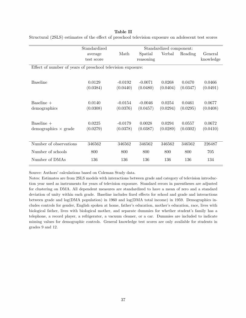
Table IIStructural (2SLS) estimates of the e¤ect of preschool television exposure on adolescent test scores
Standardized Standardized component:average Math Spatial Verbal Reading Generaltest score reasoning knowledge
E¤ect of number of years of preschool television exposure:
Baseline 0.0129 -0.0192 -0.0071 0.0268 0.0470 0.0466(0.0384) (0.0440) (0.0480) (0.0404) (0.0347) (0.0491)
Baseline + 0.0140 -0.0154 -0.0046 0.0254 0.0461 0.0677demographics (0.0308) (0.0376) (0.0457) (0.0294) (0.0295) (0.0408)
Baseline + 0.0225 -0.0179 0.0028 0.0294 0.0557 0.0672demographics � grade (0.0279) (0.0378) (0.0387) (0.0289) (0.0302) (0.0410)
Number of observations 346562 346562 346562 346562 346562 226487
Number of schools 800 800 800 800 800 705
Number of DMAs 136 136 136 136 136 134
Source: Authors�calculations based on Coleman Study data.Notes: Estimates are from 2SLS models with interactions between grade and category of television introduc-tion year used as instruments for years of television exposure. Standard errors in parentheses are adjustedfor clustering on DMA. All dependent measures are standardized to have a mean of zero and a standarddeviation of unity within each grade. Baseline includes �xed e¤ects for school and grade and interactionsbetween grade and log(DMA population) in 1960 and log(DMA total income) in 1959. Demographics in-cludes controls for gender, English spoken at home, father�s education, mother�s education, race, lives withbiological father, lives with biological mother, and separate dummies for whether student�s family has atelephone, a record player, a refrigerator, a vacuum cleaner, or a car. Dummies are included to indicatemissing values for demographic controls. General knowledge test scores are only available for students ingrades 9 and 12.
37

Table IIIIs predicted television exposure correlated with observables?
Predicted years of television Standardized averageexposure test score(1) (2)
Male -0.00087 -0.0589(0.00090) (0.0077)
English not spoken 0.00152 -0.2046at home (0.00100) (0.0088)
Father�s education -0.00024 0.0622(index) (0.00031) (0.0018)
Mother�s education -0.00009 0.0551(index) (0.00029) (0.0017)
White 0.00184 0.4400(0.00209) (0.0334)
Lives with -0.00104 0.0862biological father (0.00063) (0.0065)
Lives with 0.00003 0.1992biological mother (0.00092) (0.0068)
Family has
Telephone 0.00198 0.1215(0.00203) (0.0090)
Record player 0.00082 0.0246(0.00077) (0.0050)
Refrigerator -0.00074 0.4555(0.00206) (0.0161)
Vacuum 0.00105 0.0696(0.00094) (0.0104)
Car 0.00062 0.0677(0.00081) (0.0105)
F (12; 135) 1.41 705.63(p� value) (0:1704) (< 0:0001)Number of observations 346562 346562Number of schools 800 800Number of DMAs 136 136
Source: Authors�calculations based on Coleman Study data.Notes: Standard errors in parentheses are adjusted for clustering on DMA. Average test score is standardizedto have a mean of zero and a standard deviation of unity within each grade. All regressions include �xede¤ects for school and grade and interactions between grade and log(DMA population) in 1960 and log(DMAtotal income) in 1959. Dummies are included to indicate missing values for demographic controls.
38

Table IVE¤ect of preschool television exposure on adolescent social and behavioral outcomes
Dependent variable E¤ect of one year of Ntelevision exposure
Number of hours spent on homework each day 0.0148 334717(0.0422)
Number of books read during summer -0.0760 336127(standardized) (0.0422)
Student sometimes feels like (s)he �just can�t learn� -0.0040 327281(0.0208)
Highest grade student wants to �nish in school -0.0265 333570(standardized) (0.0221)
Share of membership organizations 0.0170 217392(0.0398)
Source: Authors�calculations based on Coleman Study data.Notes: Estimates are from 2SLS models with interactions between grade and category of television introduc-tion year used as instruments for years of television exposure. Standard errors in parentheses are adjustedfor clustering on DMA. Standardized measures have a mean of zero and a standard deviation of unity withineach grade. Baseline includes �xed e¤ects for school and grade and interactions between grade and log(DMApopulation) in 1960 and log(DMA total income) in 1959. All regressions include controls for gender, Englishspoken at home, father�s education, mother�s education, race, lives with biological father, lives with biologicalmother, and separate dummies for whether student�s family has a telephone, a record player, a refrigerator, avacuum cleaner, or a car, as well as for interactions between grade dummies and these controls. Dummies areincluded to indicate missing values for demographic controls. Share of membership organizations is numberof the following organizations that the student belongs to, divided by the total number of organizationsfor which the student provides a response: sports team, Student Council, debate team, and hobby club.Participation in membership organizations is only available for students in grades 9 and 12.
39

Table VHeterogeneity in the e¤ects of preschool television exposure on adolescent test scores
Mother has HS degree? English at home? White?Yes No Yes No Yes No(1) (2) (3) (4) (5) (6)
E¤ect of number of years of preschool television exposure on:
Average score 0.0135 0.0418 0.0157 0.0766 0.0026 0.0526(0.0297) (0.0334) (0.0277) (0.0479) (0.0262) (0.0489)
Math -0.0477 0.0289 -0.0283 0.0352 -0.0293 -0.0055(0.0422) (0.0354) (0.0390) (0.0476) (0.0405) (0.0445)
Spatial reasoning 0.0125 -0.0342 -0.0050 0.0592 0.0225 -0.0345(0.0395) (0.0446) (0.0362) (0.0608) (0.0277) (0.0577)
Verbal 0.0308 0.0482 0.0252 0.0740 -0.0191 0.1167(0.0294) (0.0398) (0.0285) (0.0529) (0.0189) (0.0471)
Reading 0.0450 0.0942 0.0528 0.0927 0.0273 0.0922(0.0316) (0.0454) (0.0332) (0.0453) (0.0386) (0.0543)
General knowledge 0.0074 0.0657 0.0260 0.2123 -0.0945 0.1401(0.0529) (0.0487) (0.0378) (0.1551) (0.0423) (0.0786)
Number of observations:
All grades 157788 112849 280455 57514 211580 126886Grades 9-12 110805 82874 186126 36196 142328 79713
Source: Authors�calculations based on Coleman Study data.Notes: Estimates are from 2SLS models with interactions between grade and category of television introduc-tion year used as instruments for years of television exposure. Standard errors in parentheses are adjustedfor clustering on DMA. All dependent measures are standardized to have a mean of zero and a standarddeviation of unity within each grade. All speci�cations include �xed e¤ects for school and grade, interactionsbetween grade and log(DMA population) in 1960 and log(DMA total income) in 1959, controls for gender,English spoken at home, father�s education, mother�s education, race, lives with biological father, lives withbiological mother, and separate dummies for whether student�s family has a telephone, a record player, arefrigerator, a vacuum cleaner, or a car, and demographic controls interacted with grade dummies. Controlsfor variable on which the sample is split are excluded. Dummies are included to indicate missing values fordemographic controls. General knowledge test scores are only available for students in grades 9 and 12.
40
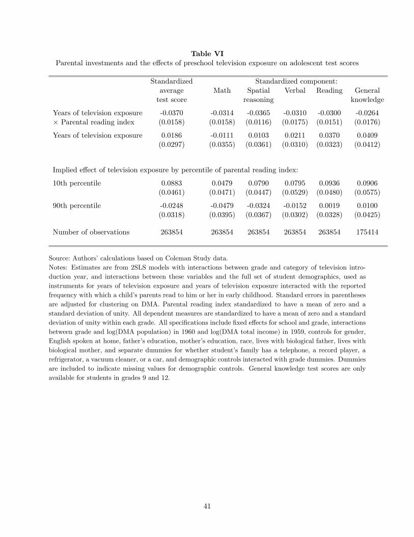
Table VIParental investments and the e¤ects of preschool television exposure on adolescent test scores
Standardized Standardized component:average Math Spatial Verbal Reading Generaltest score reasoning knowledge
Years of television exposure -0.0370 -0.0314 -0.0365 -0.0310 -0.0300 -0.0264� Parental reading index (0.0158) (0.0158) (0.0116) (0.0175) (0.0151) (0.0176)
Years of television exposure 0.0186 -0.0111 0.0103 0.0211 0.0370 0.0409(0.0297) (0.0355) (0.0361) (0.0310) (0.0323) (0.0412)
Implied e¤ect of television exposure by percentile of parental reading index:
10th percentile 0.0883 0.0479 0.0790 0.0795 0.0936 0.0906(0.0461) (0.0471) (0.0447) (0.0529) (0.0480) (0.0575)
90th percentile -0.0248 -0.0479 -0.0324 -0.0152 0.0019 0.0100(0.0318) (0.0395) (0.0367) (0.0302) (0.0328) (0.0425)
Number of observations 263854 263854 263854 263854 263854 175414
Source: Authors�calculations based on Coleman Study data.Notes: Estimates are from 2SLS models with interactions between grade and category of television intro-duction year, and interactions between these variables and the full set of student demographics, used asinstruments for years of television exposure and years of television exposure interacted with the reportedfrequency with which a child�s parents read to him or her in early childhood. Standard errors in parenthesesare adjusted for clustering on DMA. Parental reading index standardized to have a mean of zero and astandard deviation of unity. All dependent measures are standardized to have a mean of zero and a standarddeviation of unity within each grade. All speci�cations include �xed e¤ects for school and grade, interactionsbetween grade and log(DMA population) in 1960 and log(DMA total income) in 1959, controls for gender,English spoken at home, father�s education, mother�s education, race, lives with biological father, lives withbiological mother, and separate dummies for whether student�s family has a telephone, a record player, arefrigerator, a vacuum cleaner, or a car, and demographic controls interacted with grade dummies. Dummiesare included to indicate missing values for demographic controls. General knowledge test scores are onlyavailable for students in grades 9 and 12.
41

1950 penetration
0
0.05
0.1
0.15
0.2
0.25
0.3
0.35
0.4
1940
1941
1942
1945
1947
1948
1949
1950
1951
1952
1953
1954
1955
1956
+
Year of first TV station in DMA
Frac
tion
of h
hs w
ith T
V
1960 penetration
00.10.2
0.30.40.50.60.7
0.80.9
1
1940
1941
1942
1945
1947
1948
1949
1950
1951
1952
1953
1954
1955
1956
+
Year of first TV station in DMA
Frac
tion
of h
hs w
ith T
V
Figure ITelevision penetration in 1950 and 1960 by year of television introduction
Source: Television Factbooks, various years; 1950 and 1960 U.S. Censuses.Notes: The height of each bar is the fraction of households with television sets as recorded in the 1950 or1960 census, averaged over all DMAs that received television in the given year. Years in which no countyreceived its �rst station are omitted from the �gure.
42

0
0.05
0.1
0.15
0.2
0.25
0.3
0.35
1948
1949
1950
1951
1952
1953
1954
1955
1956
1957
1958
1959
1960
1961
Diff
eren
ce in
tele
visio
n pe
netr
atio
n
12thgradersborn
9thgradersborn
6thgradersborn
Figure IIDi¤erence in television penetration between early/middle and late adopters
Source: Authors�calculations.Notes: Figure is based on separate year-by-year regressions of television penetration on a dummy forearly/middle television adoption (television introduced 1952 or earlier), log income, and log population.The values plotted are the coe¢ cients on the early/middle adoption dummy. The values thus represent thedi¤erence in television penetration between early/middle adopters and late adopters in each year, adjustedfor di¤erences in log income and log population.
43

Appendix Table ISummary statistics by grade
Grade 6 Grade 9 Grade 12
Years of television exposure 3.966 3.358 1.765(0.762) (1.210) (1.194)
Year of television introductionEarly (1947 or earlier) 27% 29% 27%Middle (1948-1952) 37% 34% 34%Late (1952 or later) 37% 37% 39%
Father�s education (1 to 5) 4.041 3.898 3.793(1.992) (1.846) (1.859)
Mother�s education (1 to 5) 3.986 3.820 3.785(1.762) (1.532) (1.529)
Male 51% 51% 49%English not spoken at home 18% 17% 15%White 59% 62% 67%Lives with biological father 74% 74% 76%Lives with biological mother 89% 90% 91%
Family hasTelephone 75% 79% 85%Record player 81% 87% 89%Refrigerator 93% 97% 98%Vacuum 70% 73% 78%Car 83% 84% 88%
Number of observations 120075 131074 95413
Source: Authors�calculations based on Coleman Study data.Notes: Standard deviations in parentheses. Table displays the mean value of each variable excluding observa-tions for which the variable is missing. Percentages refer to the share of students with the given characteristicswithin each grade.
44

Appendix Table IIThe correlates of television viewing intensity
Number of hours of Standardized averagetelevision viewing test score
(1) (2)
Male 0.0415 -0.0589(0.0080) (0.0077)
English not spoken 0.0009 -0.2046at home (0.0104) (0.0088)
Father�s education -0.0509 0.0622(index) (0.0034) (0.0018)
Mother�s education -0.0306 0.0551(index) (0.0043) (0.0017)
White -0.1750 0.4400(0.0241) (0.0334)
Lives with -0.0537 0.0862biological father (0.0071) (0.0065)
Lives with 0.1029 0.1992biological mother (0.0107) (0.0068)
Family has
Telephone 0.1199 0.1215(0.0147) (0.0090)
Record player 0.1716 0.0246(0.0083) (0.0050)
Refrigerator 0.3482 0.4555(0.0320) (0.0161)
Vacuum -0.0085 0.0696(0.0114) (0.0104)
Car 0.0446 0.0677(0.0137) (0.0105)
F (12; 135) 236.09 705.63(p� value) (< 0:0001) (< 0:0001)
Number of observations 335981 346562Number of schools 800 800Number of DMAs 136 136
Source: Authors�calculations based on Coleman Study data.Notes: Standard errors in parentheses are adjusted for clustering on DMA. Average test score is standardizedto have a mean of zero and a standard deviation of unity within each grade. All regressions include �xede¤ects for school and grade and interactions between grade and log(DMA population) in 1960 and log(DMAtotal income) in 1959. Dummies are included to indicate missing values for demographic controls.
45

Appendix Table IIIHeterogeneity in television e¤ects adjusted for penetration and hours
Standardized Standardized component:average Math Spatial Verbal Reading Generaltest score reasoning knowledge
Unadjusted estimatesDoes mother have high school degree?
Yes 0.0135 -0.0477 0.0125 0.0308 0.0450 0.0074(0.0297) (0.0422) (0.0395) (0.0294) (0.0316) (0.0529)
No 0.0418 0.0289 -0.0342 0.0482 0.0942 0.0657(0.0334) (0.0354) (0.0446) (0.0398) (0.0454) (0.0487)
Adjusted for di¤erences in average television penetration, 1949-1955Does mother have high school degree?Yes 0.0117 -0.0414 0.0108 0.0267 0.0390 0.0064(Share with TV = 0.43) (0.0258) (0.0366) (0.0343) (0.0255) (0.0274) (0.0459)
No 0.0469 0.0324 -0.0383 0.0540 0.1056 0.0737(Share with TV = 0.34) (0.0375) (0.0397) (0.0500) (0.0447) (0.0509) (0.0546)
Adjusted for di¤erences in average daily preschool viewing hours and television penetrationDoes mother have high school degree?
Yes 0.0124 -0.0439 0.0115 0.0283 0.0414 0.0068(Average hours = 1.30) (0.0273) (0.0388) (0.0364) (0.0271) (0.0291) (0.0487)
No 0.0459 0.0318 -0.0376 0.0530 0.1035 0.0722(Average hours = 1.41) (0.0367) (0.0389) (0.0490) (0.0438) (0.0499) (0.0535)
Source: Authors�calculations based on Coleman Study data.Notes: Estimates are from 2SLS models with samples split by mother�s education. Standard errors inparentheses are adjusted for clustering on DMA. All dependent measures are standardized to have a meanof zero and a standard deviation of unity within each grade. All speci�cations include �xed e¤ects for schooland grade, interactions between grade and log(DMA population) in 1960 and log(DMA total income) in1959, controls for gender, English spoken at home, father�s education, race, lives with biological father,lives with biological mother, and separate dummies for whether student�s family has a telephone, a recordplayer, a refrigerator, a vacuum cleaner, or a car, and demographic controls interacted with grade dummies.Dummies are included to indicate missing values for demographic controls. General knowledge test scoresare only available for students in grades 9 and 12.
46