PRESCISION X-RAY DIFFRACTION...2015/02/03 · Figure 5: Intensity vs. Wavelength for X-Ray Diffraction using a 90Cu-10Ni sample. This sample first cleaned, then scanned. The later

$Page 1: PRESCISION X-RAY DIFFRACTION...2015/02/03 · Figure 5: Intensity vs. Wavelength for X-Ray Diffraction using a 90Cu-10Ni sample. This sample first cleaned, then scanned. The later$
LAB 03 PRECISION X-RAY DIFFRACTOMETRY SHILPIKA CHOWDHURY

Page 1 of 14

LAB 03 PRESCISION X-RAY DIFFRACTION

REPORT BY: SHILPIKA CHOWDHURY TEAM MEMBER NAME: Ashley Tsai & Jacqueline Ko LAB SECTION No. 105 GROUP 2 EXPERIMENT DATE: Mar. 4, 2014 SUBMISSION DATE: Mar. 18, 2014


Page 2 of 14

ABSTRACT The goal of this lab was to determine the lattice parameter of a Cu-Ni alloy system in order to confirm the composition of the tested alloy. In this lab, the lattice parameters of seven separate samples were determined and used to confirm the expected Cu-Ni ratios of 100 Cu, 90-10Cu-Ni, 75-25 Cu-Ni, 50-50 Cu-Ni, 20-80 Cu_Ni, 10-90 Cu-Ni, and 100 Ni. These parameters were 2.3613 Å, 2.6047 Å, 2.7346 Å, 2.4316 Å, 2.4136 Å, 2.7105 Å, and 2.7054 Å respectively. There was definitely fluctuations in the data which were not entirely smooth. This may have implied that the composition of each specimen was not what it was expected to be, or there was experimental error.

INTRODUCTION X-Ray diffractometers can be used to collect many types of information, one of which is the lattice parameter of a crystal structure. This is done by scattering a Cu-Kα x-ray beam along a single axis of a sample and determining the diffraction peaks. These peaks can be processed to not only indicate a likely structure for the specimen, but also the specific lattice parameter of that sample. The expected structure can be derived from Bragg’s Law:

And the value of a within the plane spacing term can elucidate the lattice parameters of the sample, given that the form of a plane spacing calculation is known. In the case of Copper and Nickel and any Copper-Nickel alloys, the spacing aligns with that expected of a FCC structure. Thus, the value of the plane spacing is calculated by

And the lattice parameter is

From the calculated lattice parameters, it is possible to confirm the alloy composition of a specimen by comparing a values with those expected for Copper and Nickel. It is important to also note the highest sample sensitivity is at higher diffraction angles, which can be seen after the differentiation of Bragg’s law. From here, the precision of the parameter can be evaluated using the Nelson-Riley function, and a map of the sample composition values can be constructed.


Page 3 of 14

EXPERIMENTAL PROCEDURES For this experiment, our materials were an x–ray diffractometer with a copper target, seven specimen samples (50-50 Cu-Ni, 100 Cu, 90-10Cu-Ni, 75-25 Cu-Ni, 50-50 Cu-Ni, 20-80 Cu_Ni, 10-90 Cu-Ni, and 100 Ni) and diamond paste for polishing. Before beginning both sections of the lab, we initialized the Rigaku Miniflex II X-Ray Diffractometer. This included turning on the cooling water, initializing the data collection software, and checking for background radiation. The voltage for this diffractometer is preset at 30kV and 15 mA.

EXPLORATORY SCAN A 50-50 Cu-Ni sample was packed and loaded into the diffractometer. The first sample was run without polishing in order to determine peak regions. Therefore this scan was run over a 2θ range of 3° to 140° at 6°/sec.

PEAK COLLECTION After determining the approximate location of diffraction peaks, the peaks were scanned at high precision at each peak locus, tabulated below. Specific 2θ values are listed. The peak collection was limited to the last 5 peaks as those peaks would contribute the highest precision to the lattice parameter calculation. The peaks were collected at a slow rate of 0.5°/sec. For our precise data, we then collected peaks for diamond paste polished 50-50 Cu-Ni, unpolished and polished pure Cu and pure Nickel, and then polished 90-10Cu-Ni, 75-25 Cu-Ni, 50-50 Cu-Ni, 20-80 Cu_Ni, and 10-90 Cu-Ni. These values were over the data ranges tabulated in Table 1. Table 1: 2θB Ranges for each sample, determined with a guess-and-check process. Certain samples were not ideal for certain peaks, but nearly all samples had 5 workable peaks. Only the 20Cu-80Ni and 90Cu-10Ni samples had fewer. All table headings are in Cu-Ni ratio format.

Peak hkl 50-50 2θ 100 Cu 2θ 90-10 2θ 75-25 2θ 20-80 2θ 10-90 2θ 100 Ni 2θ

1 111 - - - - 43-46° - - 2 200 - 48-52° 51-52° 49-52.5° 50-53° 50-53.5° 50-53° 3 220 74-77° 75-80° - 73-76.5° 74-77° 74-77° 75-78° 4 311 90-93° - 92-93° 89-92.5° 91-94° 91-94° 92-94° 5 222 95-98° 88-98° - 96-98° - 95-100° 98-100° 6 400 117-121° 116-125° 117-119° 116-119° - 120-123° 121-123° 7 331 139-143° 138-145° 137-139° - - - -


Page 4 of 14

EXPERIMENTAL RESULTS In all x–ray experiments, the background radiation was found to be 0.02 mR/hr using a Geiger counter during x–ray emission and before emission.

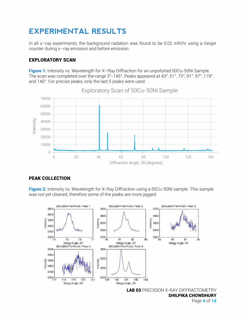
EXPLORATORY SCAN Figure 1: Intensity vs. Wavelength for X–Ray Diffraction for an unpolished 50Cu-50Ni Sample. The scan was completed over the range 3°-145°. Peaks appeared at 43°, 51°, 75°, 91°, 97°, 119°, and 140°. For precise peaks, only the last 5 peaks were used.

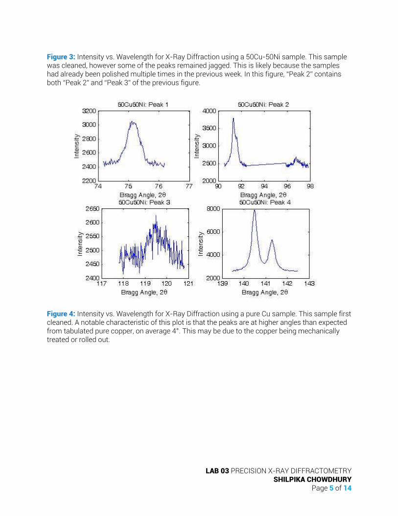
PEAK COLLECTION Figure 2: Intensity vs. Wavelength for X-Ray Diffraction using a 50Cu-50Ni sample. This sample was not yet cleaned, therefore some of the peaks are more jagged.

0

10000

20000

30000

40000

50000

60000

70000

3 23 43 63 83 103 123 143

Inte

ns

ity

Diffraction Angle, 2θ (degrees)

Exploratory Scan of 50Cu-50Ni Sample


Page 5 of 14

Figure 3: Intensity vs. Wavelength for X-Ray Diffraction using a 50Cu-50Ni sample. This sample was cleaned, however some of the peaks remained jagged. This is likely because the samples had already been polished multiple times in the previous week. In this figure, “Peak 2” contains both “Peak 2” and “Peak 3” of the previous figure.

Figure 4: Intensity vs. Wavelength for X-Ray Diffraction using a pure Cu sample. This sample first cleaned. A notable characteristic of this plot is that the peaks are at higher angles than expected from tabulated pure copper, on average 4°. This may be due to the copper being mechanically treated or rolled out.


Page 6 of 14

Figure 5: Intensity vs. Wavelength for X-Ray Diffraction using a 90Cu-10Ni sample. This sample first cleaned, then scanned. The later peaks appear to be very jagged, so maximum values/peak values were determined by inspection rather than the overall maximum intensity over the range.

Figure 6: Intensity vs. Wavelength for X-Ray Diffraction using a 75Cu-25Ni sample. This sample first cleaned. The polishing on this sample immensely improved the peak quality. Another factor in the quality may have been the diffractometer on which the data was collected on, as this sample was collected on a different diffractometer than some of the other samples.


Page 7 of 14

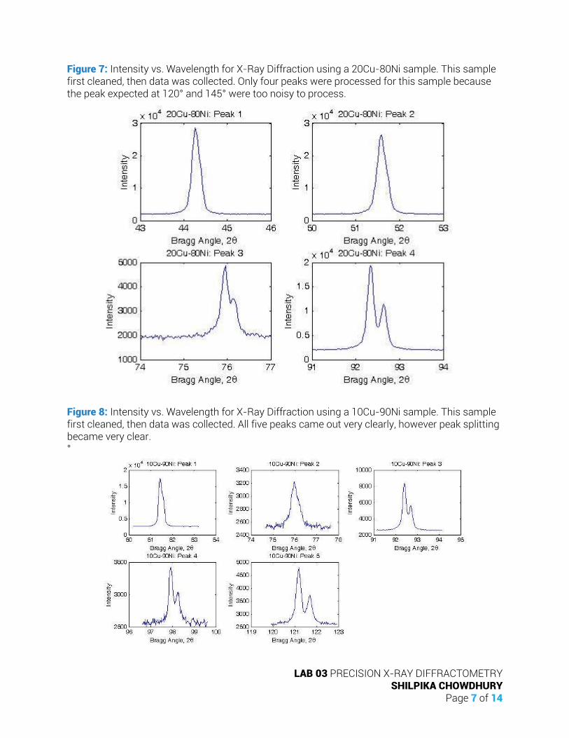
Figure 7: Intensity vs. Wavelength for X-Ray Diffraction using a 20Cu-80Ni sample. This sample first cleaned, then data was collected. Only four peaks were processed for this sample because the peak expected at 120° and 145° were too noisy to process.

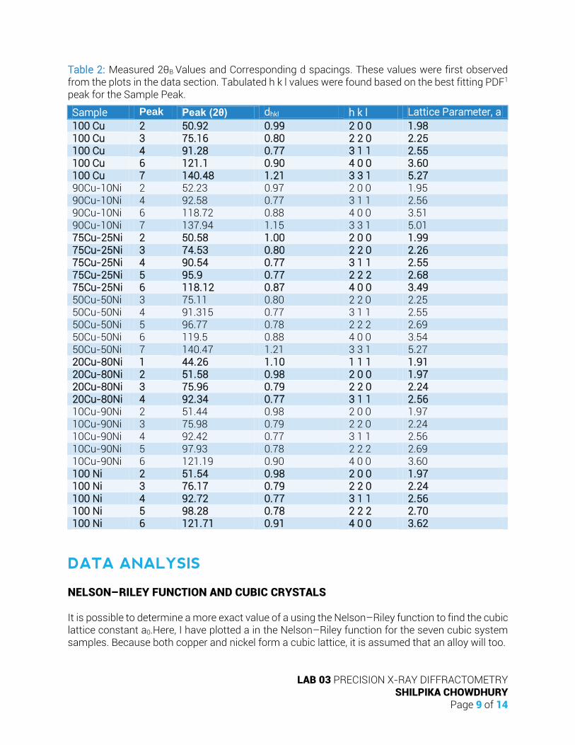
Figure 8: Intensity vs. Wavelength for X-Ray Diffraction using a 10Cu-90Ni sample. This sample first cleaned, then data was collected. All five peaks came out very clearly, however peak splitting became very clear. °


Page 8 of 14

Figure 9: Intensity vs. Wavelength for X-Ray Diffraction using a Pure Ni sample. This sample first cleaned, then data was collected. Only five peaks were processed for this sample because the peak expected at 145° was too noisy to process. The peak at 120° is also very noisy, but the maximum intensity value was still used as peak height and centering.

DISCUSSION Our results displayed significant peaks which we were able to use to confirm the identities of the samples which we worked with. Further, we were able to determine a likely lattice parameter for each of the samples.

DATA REDUCTION OBSERVATIONS The peaks in each sample were tabulated in Table 2, then the d-plane spacing and hkl indices were determined. From the spacing and hkl values, the lattice parameter a could also be tabulated. In a cubic system, the structure of the relationship dhkl and h, k and l is written as:

Where a is the lattice parameter. If we rearrange, we can find an equation for lattice spacing in terms of our known values.


Page 9 of 14

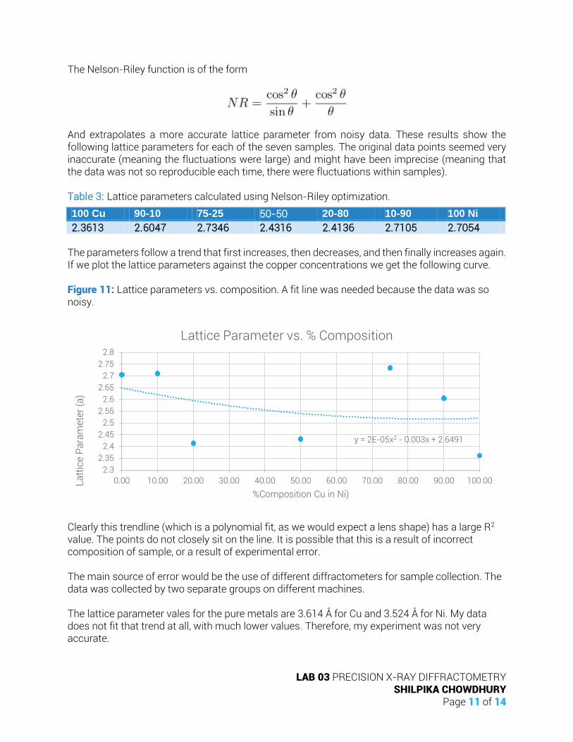
Table 2: Measured 2θB Values and Corresponding d spacings. These values were first observed from the plots in the data section. Tabulated h k l values were found based on the best fitting PDF1 peak for the Sample Peak.

Sample Peak Peak (2θ) dhkl h k l Lattice Parameter, a

100 Cu 2 50.92 0.99 2 0 0 1.98 100 Cu 3 75.16 0.80 2 2 0 2.25 100 Cu 4 91.28 0.77 3 1 1 2.55 100 Cu 6 121.1 0.90 4 0 0 3.60 100 Cu 7 140.48 1.21 3 3 1 5.27 90Cu-10Ni 2 52.23 0.97 2 0 0 1.95 90Cu-10Ni 4 92.58 0.77 3 1 1 2.56 90Cu-10Ni 6 118.72 0.88 4 0 0 3.51 90Cu-10Ni 7 137.94 1.15 3 3 1 5.01 75Cu-25Ni 2 50.58 1.00 2 0 0 1.99 75Cu-25Ni 3 74.53 0.80 2 2 0 2.26 75Cu-25Ni 4 90.54 0.77 3 1 1 2.55 75Cu-25Ni 5 95.9 0.77 2 2 2 2.68 75Cu-25Ni 6 118.12 0.87 4 0 0 3.49 50Cu-50Ni 3 75.11 0.80 2 2 0 2.25 50Cu-50Ni 4 91.315 0.77 3 1 1 2.55 50Cu-50Ni 5 96.77 0.78 2 2 2 2.69 50Cu-50Ni 6 119.5 0.88 4 0 0 3.54 50Cu-50Ni 7 140.47 1.21 3 3 1 5.27 20Cu-80Ni 1 44.26 1.10 1 1 1 1.91 20Cu-80Ni 2 51.58 0.98 2 0 0 1.97 20Cu-80Ni 3 75.96 0.79 2 2 0 2.24 20Cu-80Ni 4 92.34 0.77 3 1 1 2.56 10Cu-90Ni 2 51.44 0.98 2 0 0 1.97 10Cu-90Ni 3 75.98 0.79 2 2 0 2.24 10Cu-90Ni 4 92.42 0.77 3 1 1 2.56 10Cu-90Ni 5 97.93 0.78 2 2 2 2.69 10Cu-90Ni 6 121.19 0.90 4 0 0 3.60 100 Ni 2 51.54 0.98 2 0 0 1.97 100 Ni 3 76.17 0.79 2 2 0 2.24 100 Ni 4 92.72 0.77 3 1 1 2.56 100 Ni 5 98.28 0.78 2 2 2 2.70 100 Ni 6 121.71 0.91 4 0 0 3.62

DATA ANALYSIS NELSON–RILEY FUNCTION AND CUBIC CRYSTALS It is possible to determine a more exact value of a using the Nelson–Riley function to find the cubic lattice constant a0.Here, I have plotted a in the Nelson–Riley function for the seven cubic system samples. Because both copper and nickel form a cubic lattice, it is assumed that an alloy will too.


Page 10 of 14

Figure 10: Nelson – Riley function vs. lattice parameter in cubic samples. A Sample 1 B Sample 2 C Sample 3 D Sample 4 E Sample 5 F Sample 6 G Sample 7. The a0 value determined by plotting these points gives us the most accurate value of a.

y = 1.4317x + 2.3613

0.00

1.00

2.00

3.00

4.00

5.00

6.00

0 0.5 1 1.5 2

a (

Å)

Nelson-Riley

A Sample 1

y = 1.1261x + 2.6047

0.00

1.00

2.00

3.00

4.00

5.00

6.00

0 0.5 1 1.5 2

a (

Å)

Nelson-Riley

A Sample 2

y = -0.4663x + 2.7346

0.00

1.00

2.00

3.00

4.00

0 0.5 1 1.5 2

a (

Å)

Nelson-Riley

C Sample 3

y = 2.4204x + 2.4316

0

1

2

3

4

5

6

0 0.5 1 1.5 2

a (

Å)

Nelson-Riley

D Sample 4

y = -0.4022x + 2.4136

0.00

0.50

1.00

1.50

2.00

2.50

3.00

0 0.5 1 1.5 2

a (

Å)

Nelson-Riley

E Sample 5

y = -0.3242x + 2.7105

0

1

2

3

4

0 0.5 1 1.5 2

a (

Å)

Nelson-Riley

F Sample 6

y = -0.2933x + 2.7054

0.00

1.00

2.00

3.00

4.00

0 0.5 1 1.5 2

a (

Å)

Nelson-Riley

G Sample 7


Page 11 of 14

The Nelson-Riley function is of the form

And extrapolates a more accurate lattice parameter from noisy data. These results show the following lattice parameters for each of the seven samples. The original data points seemed very inaccurate (meaning the fluctuations were large) and might have been imprecise (meaning that the data was not so reproducible each time, there were fluctuations within samples). Table 3: Lattice parameters calculated using Nelson-Riley optimization.

100 Cu 90-10 75-25 50-50 20-80 10-90 100 Ni

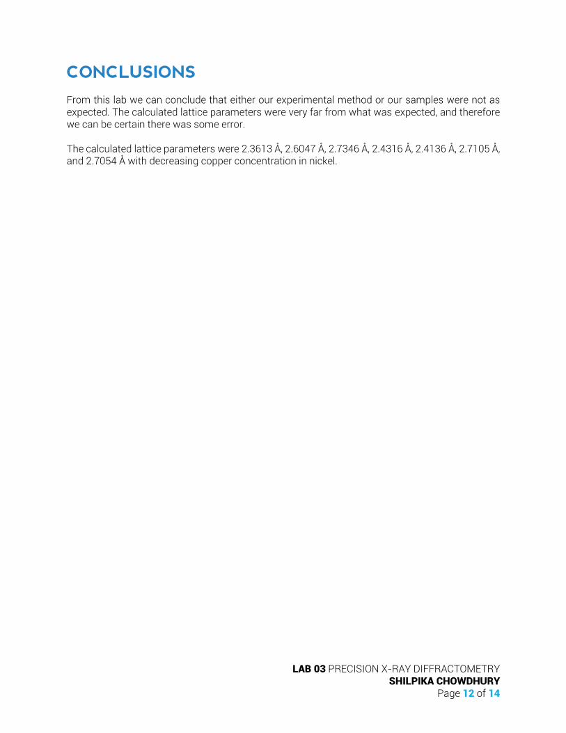
2.3613 2.6047 2.7346 2.4316 2.4136 2.7105 2.7054 The parameters follow a trend that first increases, then decreases, and then finally increases again. If we plot the lattice parameters against the copper concentrations we get the following curve. Figure 11: Lattice parameters vs. composition. A fit line was needed because the data was so noisy.

Clearly this trendline (which is a polynomial fit, as we would expect a lens shape) has a large R2 value. The points do not closely sit on the line. It is possible that this is a result of incorrect composition of sample, or a result of experimental error. The main source of error would be the use of different diffractometers for sample collection. The data was collected by two separate groups on different machines. The lattice parameter vales for the pure metals are 3.614 Å for Cu and 3.524 Å for Ni. My data does not fit that trend at all, with much lower values. Therefore, my experiment was not very accurate.

y = 2E-05x2 - 0.003x + 2.6491

2.3

2.35

2.4

2.45

2.5

2.55

2.6

2.65

2.7

2.75

2.8

0.00 10.00 20.00 30.00 40.00 50.00 60.00 70.00 80.00 90.00 100.00La

ttic

e P

ara

me

ter

(a)

%Composition Cu in Ni)

Lattice Parameter vs. % Composition


Page 12 of 14

CONCLUSIONS From this lab we can conclude that either our experimental method or our samples were not as expected. The calculated lattice parameters were very far from what was expected, and therefore we can be certain there was some error. The calculated lattice parameters were 2.3613 Å, 2.6047 Å, 2.7346 Å, 2.4316 Å, 2.4136 Å, 2.7105 Å, and 2.7054 Å with decreasing copper concentration in nickel.


Page 13 of 14

REFERENCES

1 R. Gronsky. Lab 02 Manual: Powder Diffraction. MSE 104. University of California Berkeley, Berkeley, CA.

2 B.D. Cullity and S.R. Stock, Elements of X-Ray Diffraction, 3rd Edition, Prentice-Hall, New York, (2001), Appendix 3, p. 619.


Page 14 of 14

APPENDIX Overflow materials should appear here. Examples include extra data runs, problematic data (such as interrupted data runs), copies of pertinent literature or other documentation, computer source code listings, or derivations of equations. No additional Information was required.

Documents

PRESCISION X-RAY DIFFRACTION...2015/02/03 · Figure 5: Intensity vs. Wavelength for X-Ray Diffraction using a 90Cu-10Ni sample. This sample first cleaned, then scanned. The later