Embed Size (px)
Citation preview

TRACKING ACCURACY OF 3.6 METER TELESCOPE AT DEVASTHAL AND
TEMPERATURE PLOT & OPTICAL DEPTH OF STAR FORMING MOLECULAR CLOUDS FROM
PLANCK SATELLITE DATANIKHIL S HUBBALLI
GUIDE:
DR. MAHESWAR GOPINATHAN (ARIES, NAINITAL)

PART – ITRACKING ACCURACY OF 3.6 METER TELESCOPE AT
DEVASTHAL

INTRODUCTION
• Observations in astronomy
• Need for tracking objects in the sky with time
• Earth’s rotation relative to stars (solar day – 86400 sec, sidereal day – 86164 sec)
• Telescope RA axis must rotate in sync with earth’s sidereal time period
• Drifts in the images of long exposure observations of objects
• Reasons:
Inaccurate polar alignment
Incorrect RA motor speed
Periodic error in RA
• Mechanical systems that track objects perfectly is not possible, it’ll be associated with errors
• So, RMS tracking error specifications are tried to be met for the systems
• An analysis is done on the telescopic data of different exposures covering various azimuth and altitude locations

AIM
• Analyse the centroid position variations through entire image frames over considered exposure time
• Based on the specifications of the telescope mechanical systems, it is required to have the tracking accuracy <0.1 arcsec RMS for less than one minute in closed loop for wind inside the dome <3m/s and <0.11 arcsec RMS for less than one hour in closed loop for wind inside the dome <3m/s
• From the plots obtained for RMS tracking error, it’s required to get the tracking error under specification for entire sky coverage

INSTRUMENTS
• Test camera used : MICROLINE ML 402ME
• CCD pixel size : 9*9 μm2
• CCD read noise : 15 electrons
• CCD dark current : 0.5 e/s/pixel
• Air cooled
• Waveband : 550nm – 750 nm
• CCD QE : 70% (550nm), 80% (650nm), 60% (750nm)
• Field of view : 0.05768 arcsec/pixel

TELESCOPIC DATA
Main Port – Closed loop
• Measurement 1 - Alt [deg] : 63 to 50 • Az [deg] : -56 to -59 • Acquisition time : 30 s
• Measurement 2 - Alt [deg] : 79 to 75 • Az [deg] : 20 to -35 • Acquisition time : 30 s
• Measurement 3 - Alt [deg] : 30 to 41 • Az [deg] : 124 to 138 • Acquisition time : 30 s
• Measurement 4 (10 arcmin Field of view radius) - Alt [deg] : 87 to 75 • Az [deg] : 0 to -70 • Acquisition time : 30 s
Side Port 1 – Closed loop
• Measurement 1 - Alt [deg] : 47 to 32 • Az [deg] : -75 to -70 • Acquisition time : 30 s
• Measurement 2 - Alt [deg] : 56 to 70 • Az [deg] : 86 to 94 • Acquisition time : 30 s
• Measurement 3 - Alt [deg] : 33 to 26 • Az [deg] : -57 to -55 • Acquisition time : 30 s
• Measurement 4 - Alt [deg] : 80.5 to 82 • Az [deg] : 25 to -30 • Acquisition time : 30 s

TELESCOPIC DATA
Side Port 2 – Closed loop
• Measurement 1 - Alt [deg] : 55 to 40 • Az [deg] : -118 to -104 • Acquisition time : 30 s
• Measurement 2 - Alt [deg] : 32 to 48 • Az [deg] : 86 to 96 • Acquisition time : 30 s
• Measurement 3 - Alt [deg] : 87 to 73 • Az [deg] : 200 to 260 • Acquisition time : 30 s
• Measurement 4 - Alt [deg] : 53 to 49 • Az [deg] : -10 to -20 • Acquisition time : 30 s
The data was made available for the analysis by the team at Devasthal. The observations were made in November and December, 2015

APPROACH
• Observations are CCD images. There are many frames with certain exposure time.
• Because of errors in tracking, the position of star in the image will have shifted compared to the previous frame
• To find the error in tracking, centroid in each of the frame is calculated
• The simplest approach in finding the centroid is Marginal sums approach or first moment distributions approach

FINDING CENTROID OF THE IMAGE• Consider an image with dimensions 2L+1 * 2L+1, where L is comparable to the size of star in the
frame
• Marginal distributions of the star in the images is found using:
𝐼𝑖 = 𝑗=−𝐿𝑗=𝐿𝐼𝑖, 𝑗 and 𝐽𝑗 = 𝑖=−𝐿
𝑖=𝐿 𝐽𝑖, 𝑗
𝐼𝑖, 𝑗 is the intensity (in ADU) at each x, y pixel
• The mean intensities are determined from:
𝐼 =1
2𝐿+1 𝑖=−𝐿𝑖=𝐿 𝐼𝑖 and 𝐽 =
1
2𝐿+1 𝑗=−𝐿𝑗=𝐿𝐽𝑗
• Finally, intensity weighted centroid is calculated using:
𝑥𝑐 = 𝑖=−𝐿𝑖=𝐿 𝐼
𝑖− 𝐼 𝑥
𝑖
𝑖=−𝐿𝑖=𝐿 𝐼
𝑖− 𝐼
and y𝑐 = 𝑗=−𝐿𝑗=𝐿
𝐽𝑗− 𝐽 𝑦
𝑗
𝑗=−𝐿𝑗=𝐿
𝐽𝑗− 𝐽

CENTROID VARIATION
• Centroid algorithm is applied to all the frames and x, y coordinates of centroid is found out in terms of pixel positions and then converted to arcsec.
• Moving averages over 30 sec is calculated for both x, y coordinate values
• To see the centroid position variation, a plot between moving average data for x, y coordinate versus entire time range is plotted

RMS ERROR IN TRACKING
• RMS error is calculated over different exposure time
• For RMS on 1 min, we consider moving averages over 30 sec for the frames which make up to 1 min of exposure time in both x, y coordinates
• Standard deviation is calculated in each x and y coordinates from the moving averages at each exposure of 1 min considered
• From the standard deviation values in x and y coordinates, RMS error is calculated as
𝑅𝑀𝑆 = 𝑥2 + 𝑦2
• These RMS errors in each interval of 1 min are calculated over entire span of observation data
• The procedure is extended to RMS on 30 min and RMS on 50 min

RESULTS AND ANALYSIS
• Following the procedure, for each of the observation measurement two different plots are plotted
• Centroid Variation in x, y coordinates ( with zero-mean error)
• RMS tracking error (on 1 min, 30 min, 50 min)

MAIN PORT-CLOSED LOOPMEASUREMENT 1: 20151130-200400-TCAM-MP-CL
Total number of frames: 1679, Exposure : 2 sec, Total time : 3358 sec (55.96 min)RMS error on 1 min : 0.046 arcsec • RMS error on 30 min : 0.073 arcsec • RMS error on 50 min : 0.072 arcsec

MEASUREMENT 2: 20151130-212600-TCAM-MP-CL
Total number of frames: 4315, Exposure : 0.5 sec, Total time : 2157.5 sec (35.958 min)RMS error on 1 min : 0.028 arcsec • RMS error on 30 min : 0.08 arcsec

MEASUREMENT 3: 20151130-224500-TCAM-MP-CL
Total number of frames: 730, Exposure : 8 sec (frame 1-209 ), 4 sec (frame 210-730), Total time : 3756 sec (62.6 min)RMS error on 1 min : 0.054 arcsec • RMS error on 30 min : 0.078 arcsec • RMS error on 50 min : 0.082 arcsec

MEASUREMENT 4: 20151202-234800-TCAM-MP-CL
Total number of frames: 627, Exposure : 6 sec, Total time : 3762 sec (62.7 min)RMS error on 1 min : 0.06 arcsec • RMS error on 30 min : 0.08 arcsec • RMS error on 50 min : 0.079 arcsec

SIDE PORT 1 - CLOSED LOOPMEASUREMENT 1: 20151107-031900-TCAM-SP1-CL
Total number of frames: 1163, Exposure : 3 sec, Total time : 3489 sec (58.15 min)RMS error on 1 min : 0.057 arcsec • RMS error on 30 min : 0.087 arcsec • RMS error on 50 min : 0.098 arcsec

MEASUREMENT 2: 20151107-194900-TCAM-SP1-CL
Total number of frames: 1964, Exposure : 3 sec (frame 1-124), 1.5 sec (frame 125-1964), Total time : 3132 sec (52.2 min)RMS error on 1 min : 0.039 arcsec • RMS error on 30 min : 0.053 arcsec • RMS error on 50 min : 0.057 arcsec

MEASUREMENT 3: 20151108-001400-TCAM-SP1-CL
Total number of frames: 851, Exposure : 4 sec, Total time : 3404 sec (56.73 min)RMS error on 1 min : 0.069 arcsec • RMS error on 30 min : 0.107 arcsec • RMS error on 50 min : 0.099 arcsec

MEASUREMENT 4: 20151108-014000-TCAM-SP1-CL
Total number of frames: 1158, Exposure : 3 sec, Total time : 3474 sec (57.9 min)RMS error on 1 min : 0.035 arcsec • RMS error on 30 min : 0.061 arcsec • RMS error on 50 min : 0.054 arcsec

SIDE PORT 2 - CLOSED LOOPMEASUREMENT 1: 20151202-021500-TCAM-SP2-CL
Total number of frames: 386, Exposure : 10 sec, Total time : 3868 sec (64.33 min)RMS error on 1 min : 0.067 arcsec • RMS error on 30 min : 0.089 arcsec • RMS error on 50 min : 0.083 arcsec
MEASUREMENT 2: 20151202-184900-TCAM-SP2-CL
Total number of frames: 706, Exposure : 5 sec, Total time : 3530 sec (58.83 min)RMS error on 1 min : 0.097 arcsec • RMS error on 30 min : 0.131 arcsec • RMS error on 50 min : 0.147 arcsec

MEASUREMENT 3: 20151202-205000-TCAM-SP2-CL
Total number of frames: 393, Exposure : 10 sec, Total time : 3930 sec (65.5 min)RMS error on 1 min : 0.062 arcsec • RMS error on 30 min : 0.075 arcsec • RMS error on 50 min : 0.074 arcsec

MEASUREMENT 4: 20151202-220600-TCAM-SP2-CL
Total number of frames: 879, Exposure : 4 sec, Total time : 3516 sec (58.6 min)RMS error on 1 min : 0.071 arcsec • RMS error on 30 min : 0.096 arcsec • RMS error on 50 min : 0.097 arcsec

CONCLUSIONS
• This analysis was meant for the telescope adjustments to get the tracking and image quality specifications. The performance have been tested on datasets Main Port, Side Port 1 and Side Port 2.
• Training related to Telescope control system, rotator, adapter and guider were not undertaken.
• A total of 12 tracking measurements have been taken altogether on all three ports, out of which there are three values 0.107, 0.131, 0.147 which are greater than the specified value of 0.1 arcsec.
• From the measurements, it can be seen that the tracking of the telescope is well within the specified values of 0.1 arcsec RMS for less than 1 min and 0.11 arcsec RMS for less than 1 hour.

PART – IITEMPERATURE PLOT & OPTICAL DEPTH OF STAR FORMING MOLECULAR CLOUDS FROM PLANCK
SATELLITE DATA

WHAT ARE MOLECULAR CLOUDS?
• A molecular cloud is an accumulation of interstellar gas and dust.
• The temperature of these clouds vary from 10 to 30 kelvin.
• Primarily, these consist of molecular hydrogen along with traces of CO and other species. Their size can be as big as 600 light years and mass as high as several million solar masses.
• The density of these regions is also high ranging in the order of 1012 particles/m3. Particles in these regions are mostly in molecular form rather than atomic, and thus these high dense regions are called molecular clouds. These molecular clouds contain enough mass to make a million stars like sun.

WHY DO WE STUDY THEM?
• Molecular clouds play an important galactic role in the formation of massive stars.
• These massive stars, formed in them, provide the main energy sources for the interstellar medium, partly by destroying their birth clouds and recycling their matter back into more diffuse forms.
• Also for understanding the dynamics of the interstellar medium and ultimately the evolution of galaxies as a whole
• Different types of molecules have been detected in the molecular clouds such as water, ammonia, ethyl alcohol, even sugar and amino acids like glycine (C2H5NO2) the basic molecules of life.
• Molecular clouds present a wide range of physical conditions (illumination, density, star-forming activity)
• Therefore they are ideal for studying the emission properties of dust grains and their evolution

UNDERSTANDING MOLECULAR CLOUDS
• Most of the mass is molecular hydrogen, but it’s invisible under quiescent interstellar conditions
• Because of this, we go for observations of emission and absorption from dust and rotational lines from species such as CO and its isotopologues.
• Help determine the properties of molecular clouds
• Dense cores exist preferentially in the small percentage of molecular clouds with high column density
• In order to understand why these dense cores form only in certain regions, how long these cores can survive without collapsing or dispersing, and a few other star formation issues, we need to determine basic properties of molecular clouds such as the temperature, optical depth, density distributions, spectral emissivity index and internal motions of the gas and dust

PLANCK SATELLITE & IRAS
• Launched in May 2009, Planck is a European Space Agency mission designed to image the temperature and polarization anisotropies of the Cosmic Background Radiation Field over the whole sky, with unprecedented sensitivity and angular resolution at microwave and infra-red frequencies.
• It has two major instruments Low Frequency instrument and High Frequency instrument
• Both instruments can detect both the total intensity and polarization of photons, and together cover a frequency range of nearly 830 GHz (from 30 to 857 GHz). The cosmic microwave background spectrum peaks at a frequency of 160.2 GHz.
• The Infrared Astronomical Satellite (IRAS) was the first-ever space-based observatory to perform a survey of the entire sky at infrared wavelengths.
• Infrared sources were observed in 12, 25, 60 and 100 µm wavelengths, with resolutions ranging from 30 arcsec at 12 µm to 2 arcmin at 100 µm.

AIM
• Creating a general tool to generate temperature plot, optical depth map, spectral emissivity index map and also the correlations of these parameters for any given molecular cloud
• Given the data of the molecular region in 6 bands of Planck HFI spectral data and also iris 100µm data from IRAS, we fit a modified blackbody curve to get the temperature at each pixel of the image corresponding to a region in the sky. This will enable further analysis and studies of molecular clouds.

DATA
• HFI data of Planck, along with iris 100µm data from IRAS is used for the analysis and generating the tool for mapping various parameters.
• The bands used are 100, 143, 217, 353, 545, 857 GHz from HFI data and 100µm band is used from IRAS.
• Data can be downloaded from Skyview – Virtual Observatory with following parameters.
Planck data, 100GHz:
• Regime : Millimeter
• Pixel scale : 1.7’ (arcmin)
• Pixel units : K (brightness temperature)
• Resolution : 10’
• Coordinate system : Galactic
• Projection : Tan

DATA
143GHz:
• Regime : Millimeter
• Pixel scale : 1.7’ (arcmin)
• Pixel units : K (brightness temperature)
• Resolution : 7.1’
• Coordinate system : Galactic
• Projection : Tan
217GHz:
• Regime : Millimeter
• Pixel scale : 1.7’ (arcmin)
• Pixel units : K (brightness temperature)
• Resolution : 5.5’
• Coordinate system : Galactic
• Projection : Tan

DATA
353GHz:
• Regime : Millimeter
• Pixel scale : 1.7’ (arcmin)
• Pixel units : K (brightness temperature)
• Resolution : 5.0’
• Coordinate system : Galactic
• Projection : Tan
545GHz:
• Regime : Millimeter
• Pixel scale : 1.7’ (arcmin)
• Pixel units : MJy/Sr (Spectral Flux density)
• Resolution : 5.0’
• Coordinate system : Galactic
• Projection : Tan

DATA
857GHz:
• Regime : Millimeter
• Pixel scale : 1.7’ (arcmin)
• Pixel units : MJy/Sr (Spectral Flux density)
• Resolution : 5.0’
• Coordinate system : Galactic
• Projection : Tan
IRAS, iris 100:
• Regime : Infrared
• Frequency :3000 GHz, Bandpass :2.5-3.6 THz
• Pixel scale : 1.5’ (arcmin)
• Pixel units : MJy/Sr (Spectral Flux density)
• Resolution : 2.0’
• Coordinate system : Galactic
• Projection : Tan

DATA FOR VALIDATION
• Taurus molecular cloud is used as the reference cloud to validate the method followed.
Name: Taurus Molecular cloud
• Reference longitude: 173.0°
• Reference latitude: -16.0°
• Dimension of the image: 700*700
• Image size (degrees): 19.833
• Pixel scale: 1.7’ (including iris 100 image)
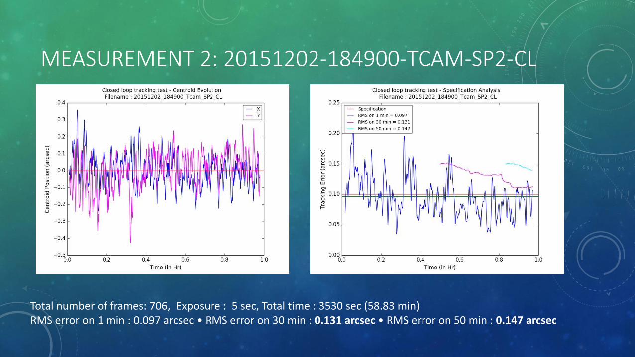
For all bands, we obtain images with size 19.833° *19.833° window centered at l = 173.0° and b = -16.0°
3000 GHZ 857 GHZ

545 GHZ 353 GHZ

217 GHZ 143 GHZ

UNIT CONVERSION
• The images of different band considered here have different pixel units.
• 100, 143, 217, 353 GHz images have brightness temperature as their pixel units where as 545, 857 GHz and iris 100 (3000GHz) images have spectral flux density as their pixel units.
• It’s necessary to find a conversion parameter between these images to have a uniform analysis
• We find that the conversion relation between brightness temperature and spectral flux density is given by:
𝑑𝑇𝑏 =𝑐2
2ν2𝑘𝑑𝐼𝑣 [Kb]

PROBLEMS OF RESOLUTION
• The data we considered have different angular resolution over different bands.
• Therefore they cannot be used for fitting the data from pixels to black body curve. It is needed to convolve the data images with their respective kernels to get images with same angular resolution, considering an image as the reference image, which is of lowest angular resolution
• For the data considered in this project, angular resolution are as follows: 100 GHz : 10’ , 143 GHz : 7.1’ , 217 GHz : 5.5’ , 353 GHz : 5.0’ , 545 GHz : 5.0’ , 857 GHz : 5.0’ , 3000 GHz (iris 100) : 2.0’
• 100 GHz data is not considered for the modified blackbody curve fit as the resolution of the images is too bad and would affect other images’ data if they are blurred to the resolution of 10’
• 143 GHz image is considered as the reference image and all the other images are blurred to the resolution of 143 GHz using convolution.
• To do this, we need to find out corresponding kernels for each of the image based on their point spread function

POINT SPREAD FUNCTION
• The point spread function (PSF) describes the response of an imaging system to a point source or point object. A more general term for the PSF is a system’s impulse response, the PSF being the impulse response of a focused optical system.
• It is considered to be the fundamental unit of an image in theoretical models of image formation.
• It is often possible to approximate the PSF (denoted by ψ) as constant across the useful field of view of the camera, so ψj(x, y, x′, y′) = ψj(x−x′, y−y′). Here S(x, y) is the source.
𝐼𝑗(𝑥, 𝑦) = 𝑆(𝑥′, 𝑦′)𝜓𝑗(𝑥 − 𝑥′, 𝑦 − 𝑦′)𝑑𝑥𝑑𝑦 = (𝑆 ⋆ 𝜓𝑗)(𝑥, 𝑦)
• PSF has normalization given by:
𝜓𝑗(𝑥, 𝑦, 𝑥′, 𝑦′)𝑑𝑥𝑑𝑦 = 1

KERNELS
• Given two cameras A and B, with PSF ψA and ψB , the images will be different for both cameras, even if the spectral responses are similar.
• A convolution kernel helps in transforming the image observed by one camera into an image corresponding to PSF of another camera.
• The convolution kernel K{A⇒B}from A to B should satisfy:
𝐾{𝐴⇒B} = FT−1 (𝐹𝑇(ψ𝐵)fA
𝐹𝑇(ψA))
Where FT is Fourier Transform, FT−1 is inverse Fourier Transform, ψA is source PSF and ψB target PSF and is fA is suitable low-pass filter

PSF GENERATION
• We generate a Gaussian beam and then for each PSF profile, we generate kernels based on the FWHM values.
• Gaussian PSF are of the form:
ψ(ϴ) =1
2πσ2exp
−ϴ2
2σ2,Where FWHM = 2σ 2 𝑙𝑛2
• Using the equation for FWHM, standard deviation for PSF of each of the image in different bands can be calculated in terms of no. of pixels
Frequency (GHz) Resolution (arcmin)
Pixel scale (arcmin/pixel)
FWHM (pixels) S.D (σ) (pixels)
143 7.1 1.7 4.1764 1.7735
217 5.5 1.7 3.2352 1.3738
353 5.0 1.7 2.9411 1.2489
545 5.0 1.7 2.9411 1.2489
857 5.0 1.7 2.9411 1.2489
3000(iris 100) 2.0 1.7 1.1764 0.4995

3000 GHZ 857 GHZ

545 GHZ 353 GHZ

217 GHZ 143 GHZ

KERNEL GENERATION
• After the PSF generation, next we have to generate corresponding kernels for convolution
• It follows these steps:
• Input the PSF and correct for missing data
• Rotate PSF (if necessary)
• Normalize the PSF
• Resample high resolution images
• Trim / Zero-pad
• Optical Transfer function
• Wiener filter
2D Laplacian operator: 0 -1 0
-1 4 -1
0 -1 0

3000 GHZ 857 GHZ

545 GHZ 353 GHZ

217 GHZ 143 GHZ

CONVOLUTION OF IMAGES
• The data images after the unit conversion in each of the band are now convolved with the corresponding kernels generated.
• The following convoluted images are obtained:

3000 GHZORIGINAL CONVOLVED

857 GHZORIGINAL CONVOLVED

545 GHZORIGINAL CONVOLVED

353 GHZORIGINAL CONVOLVED

217 GHZORIGINAL CONVOLVED

143 GHZORIGINAL CONVOLVED

APPROACH
• In the process of finding temperature plot, our main aim is to generate equations in three parameters T, τν and β and then fit the modified blackbody curve. There are two methods we can follow to achieve this:
• Pixel to pixel fitting method
• Iν (spectral flux density) equation ratio method
Here, we follow pixel to pixel fitting method.

PRINCIPLE OF SED FITTING
• The dust observed in the molecular clouds is optically thin at the observation frequencies we are considering. Therefore, its emission can be modelled as a modified black body
𝐼ν = 𝐵ν 𝑇 1 − 𝑒τν ≅ 𝐵ν 𝑇 τν
where, 𝐵ν 𝑇 is the black body function at temperature T and optical thickness τν is the power law of frequency ν,
𝐵ν 𝑇 =2ℎν3
𝑐21
𝑒ℎν𝑘𝐵𝑇𝑑 − 1
And, τν = τν0νν0
β
The frequency ν0 is an arbitrary frequency we set. Here we set ν0 = 1200 GHz

• Need to convert the measured flux into intensity
• Here, we make an assumption that temperature gradients are negligible along the line of sight
• This is an approximation - at low temperatures that characterize molecular clouds, even the small change in temperature causes large increase in the intensity.
• We receive photons from the warmer regions mostly because of which, the temperature obtained from the fit will be biased high.
• False calculations of optical depth.
• Increases as the gradient increases.
• For these regions, we consider T in equation 8.1 as effective dust temperature.

• For the process of fitting the data from IRAS and Planck , we consider a pixel position
• Spectral flux density (𝐼ν ) value is taken from all the bands at the chosen pixel position
• From the three parameters we have, (T, τν and β) we generate equations
• Using these equations we can fit a least square model to the parameters and find a single-modified blackbody curve which represents the temperature of the region the pixel corresponds to.
• We can continue this procedure for every pixel in the image to generate plots of temperature, optical depth and spectral emissivity index.

EXAMPLE FIT : MOLECULAR CLOUD REGION

EXAMPLE FIT : NON-MOLECULAR CLOUD REGION

RESULTS AND ANALYSISTAURUS MOLECULAR CLOUD – DUST TEMPERATURE MAP
REFERENCE OBTAINED

TAURUS MOLECULAR CLOUDSPECTRAL EMISSIVITY INDEX MAP
REFERENCE OBTAINED

TAURUS MOLECULAR CLOUDOPTICAL DEPTH MAP

TAURUS MOLECULAR CLOUDCORRELATION MAPS (TEMP-ΒETA)
REFERENCE OBTAINED

TAURUS MOLECULAR CLOUDHISTOGRAMS
TEMPERATURE BETA

LAMBDA - ORIONIS• Lambda Orionis is a hot, massive star that is surrounded by several other hot, massive stars, all of which
are creating radiation that excites a ring of dust, creating the "Lambda Orionis molecular ring, located at a distance of 1060 light years”
• Also called as Meissa ring
• It contains clusters of young stars and proto-stars, or forming stars, embedded within the clouds
• With a diameter of approximately 130 light-years, the Lambda Orionis molecular ring is notable for being one of the largest star-forming regions
• Data:
• Name: λ Orionis
• Reference longitude: 195.051°
• Reference latitude: -11.995°
• Dimension of the image: 700*700
• Image size (degrees): 19.833
• Pixel scale: 1.7’ (including iris 100 image)
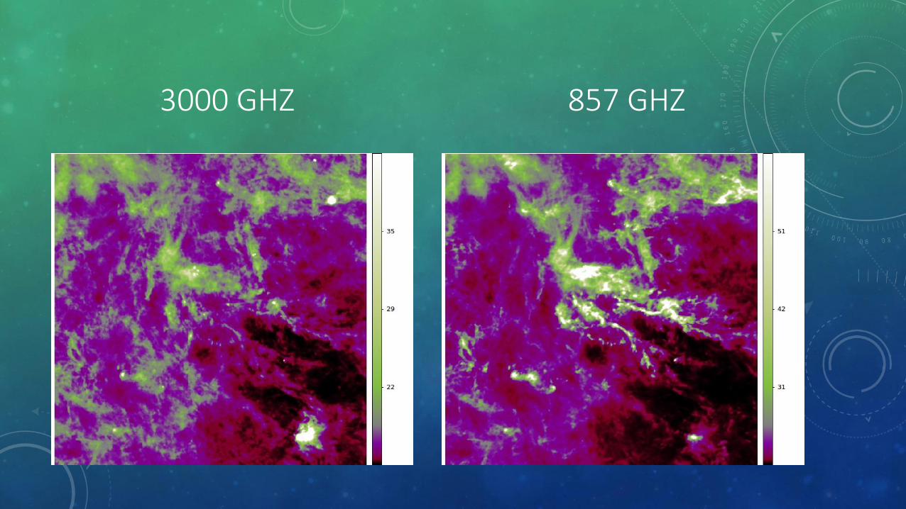
For all bands, we obtain images with size 19.833° *19.833° window centered at l = 195.051° and b = -11.995°
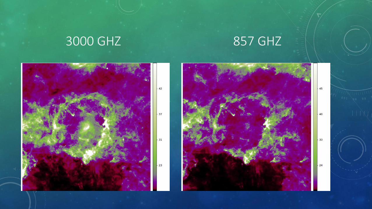
3000 GHZ 857 GHZ

545 GHZ 353 GHZ

217 GHZ 143 GHZ

LAMBDA ORIONISDUST TEMPERATURE MAP OPTICAL DEPTH MAP
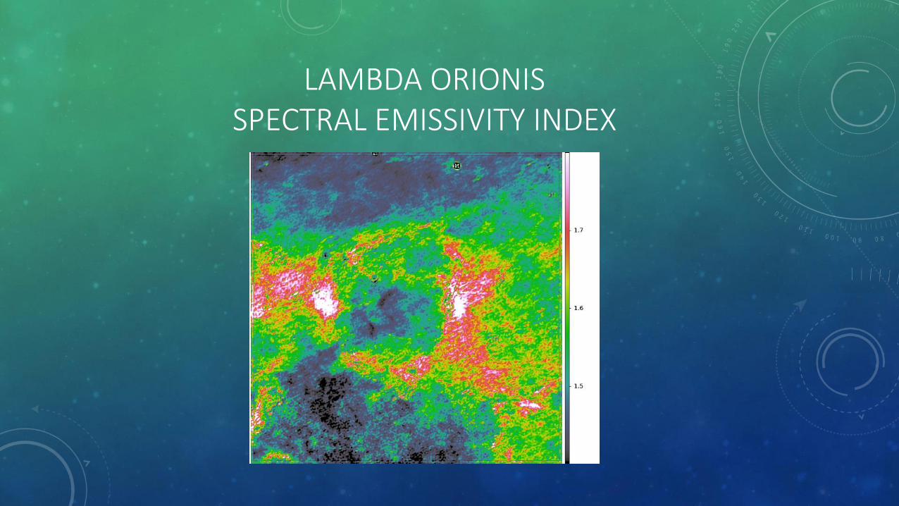
LAMBDA ORIONISSPECTRAL EMISSIVITY INDEX

LAMBDA ORIONISCORRELATION MAP (TEMP-BETA)

LAMBDA ORIONISHISTOGRAMS
TEMPERATURE BETA

PERSEUS MOLECULAR CLOUD
• The Perseus molecular cloud (Per MCld) is a nearby (600 ly) giant molecular cloud in the constellation of Perseus
• Contains over 10,000 solar masses of gas and dust covering an area of 6 by 2 degrees in the sky.
• It is very brightatmidandfar-infraredwavelengthsandinthesubmillimeteroriginatingindustheated by the newly formed low-mass stars.
• Data:
• Name: Perseus Molecular cloud
• Reference longitude: 159.450°
• Reference latitude: -19.819°
• Dimension of the image: 700*700
• Image size (degrees): 19.833
• Pixel scale: 1.7’ (including iris 100 image)
For all bands, we obtain images with size 19.833° *19.833° window centered at l = 159.450° and b = -19.819°

3000 GHZ 857 GHZ

545 GHZ 353 GHZ

217 GHZ 143 GHZ

PERSEUS MOLECULAR CLOUDDUST TEMPERATURE MAP OPTICAL DEPTH MAP

PERSEUS MOLECULAR CLOUDSPECTRAL EMISSIVITY INDEX

PERSEUS MOLECULAR CLOUDCORRELATION MAP (TEMP-BETA)

PERSEUS MOLECULAR CLOUDHISTOGRAMS
TEMPERATURE BETA
CONCLUSIONS• From temperature plot & spectral emissivity index map, we can observe that denser regions are colder
and low density regions are warmer. There are few abrupt changes in temperature, which is due to Young stellar object (YSO) sources
• We see the temperature variations mainly in 10-30 and also there’s variation in spectral emissivity index (β)
Taurus molecular cloud : 14 – 21 K (Temp); 1.6 – 1.9 (β)
λ Orionis : 16 – 27 K (Temp); 1.4 – 1.8 (β)
Perseus molecular cloud : 14 – 26 K (Temp); 1.5 – 1.85 (β)
• From the correlation plots between temperature and spectral emissivity index (β), we can see that the colder the region in the molecular cloud, higher the value of β
• Spatial distribution of column density of molecular cloud from dense to faint regions is clearly seen in the optical depth map

THANK YOU