Presentazione standard di PowerPoint - DICAT

A minimal model for flow control

with a poro-elastic coating

Divya Venkataraman, Alessandro Bottaro & Rama Govindarajan*

* On leave from JNCAS, Bangalore

ERCOFTAC Symposium on UNSTEADY SEPARATION IN

FLUID-STRUCTURE INTERACTION

Mykonos, Greece, 17-21 June 2013

WHY “POROELASTIC”?

BECAUSE IN NATURE ROUGH, COMPLIANT, FUZZY, ETC.

IS THE RULE, WHEREAS RIGID AND SMOOTH IS NOT!

Passive flow control

Problem motivation

Examples in nature abound

leading edge undulations, i.e. tubercles on whales’ flippers


Problem motivation


leading edge undulations, i.e. tubercles on whale’s flippers

multi-winglets, spiroid winglets, i.e. primary remiges


Problem motivation



multi-winglets, i.e. primary remiges

porous riblets on butterfly and moth scales (on the wings)


Problem motivation





denticles on shark skin


Problem motivation





denticles on shark skin

as well as in sports

fuzz on a tennis ball

dimples on a golf ball

...


Problem motivation

● Focus of this work: covert feathers (layer of self-actuated flaps).

● Passive “pop-up” of coverts on wings of some birds during

● landing and gliding phases of flight, perching manoeuvres;

● in general - high angle-of-attack/ low-lift regimes.

the Mykonos pelican

Passive flow control with a poro-elastic coating A rapid research survey

- Genova (at low Re number) :

Favier et al., 2009

Venkataraman & Bottaro, 2012 - Favier (AMU), Revell (Manchester), Pinelli (City U.)

Present work + Ongoing research...

- Berlin, Rechenberg,

- Freiberg, Brücker,

- Orléans, Kourta,

- Genova,

- Oxford, Taylor,

- Palaiseau, de Langre, ...

AIM: Determine structure parameters of feathers that yield “optimal” fluid-dynamical performance.

Gopinath & Mahadevan, 2010

Outline

● Computational modeling of fluid-structure interaction

➢ Highlights of numerical procedure

➢ Key computational results

● Theoretical modeling for vortex-shedding

➢ Smooth airfoil

➔ Development of the minimal model

➔ Calibration against CFD results

➢ Airfoil with poro-elastic coating (“hairfoil”)

➔ Motivation & development

➔ Results, comparison with CFD & physical indications

● Summary & future extensions

Computational modeling of fluid-structure interaction

Highlights of numerical procedure

Key computational results

Theoretical modeling for vortex-shedding

Smooth airfoil

Development of the minimal model

Calibration against CFD results

● Airfoil with poro-elastic coating (“hairfoil”)

Motivation & development

Results, comparison with CFD & physical indications

Computational model

Fluid solver (developed by Antoine Dauptain & Julien Favier)

● 2-D computations – NACA0012 airfoil.

● Re = 1100 for this study – low Reynolds number regime.

● Immersed boundary forces – for airfoil, buffer zone, coating.

● Hence, fixed Cartesian grid (fine on and near airfoil).

● Numerical scheme : ➢ Convective part - explicit Adams-Bashforth

➢ Viscous part - semi-implicit Crank-Nicolson

➢ Pressure Poisson - conjugate gradient

Mixed fluid-solid part (poro-elastic coating)

Solid body (airfoil)

Buffer zone

Validation of fluid solver Case : 10o angle of attack

● Qualitative analysis:

● Periodic solutions sinusoidal

● similar frequency spectra – peak at 2nd superharmonic of fundamental frequency.

● Quantitative analysis: Close values of

● mean lift

● frequency of oscillations.

COMPARISON OF FREQUENCY SPECTRA

● Fluid structure forcing & vice-versa

● Modeling all the feathers – too heavy.... Hence,

● Normal component of the force: Koch & Ladd (JFM, 1997)

● Tangential component: Stokes' flow approx (Favier et al. JFM, 2009)

Homogenized approach Varying porosity & anisotropy

Structure solver

● For each reference feather, equation for momentum balance solved.

● Different frequency scales (≡ time scales) :

● In present problem, rigidity effects dominant - i.e,





Smooth airfoil






RESULTS : Smooth airfoil case

Efficient structure parameters

Parameters varied during the course of the study

Parameters fixed throughout the course of the study

Summary of computational results [Phys. Fluids, 2012] ● α = 22o :

Mean lift : 34.36%, Lift fluctuations' : 7.15%, Drag fluctuations' : 35.47%, Mean drag : 6.6%

● α = 45o : ● Mean drag : 8.92%, Drag fluctuations' : 10.46%, Mean lift : 1.47%.

● α = 70o : ● Mean lift : 7.5%, Drag fluctuations' : 9.71%, Mean drag : 4.92%.





Smooth airfoil

➔ Development of the minimal model

➔ Calibration against CFD results

Airfoil with poro-elastic coating (“hairfoil”)



Minimal models: (Airfoil) Vortex-shedding

FINAL AIM: (a) predict “optimal” structure parameters at a

fraction of the cost

(b) explain physical mechanism behind such

optimal coatings

Some facts

● For unsteady flows over bodies, for fixed set of parameters, long time

history of lift/drag forces periodic + independent of initial conditions

i.e, lift/drag can be represented as self-excited oscillator,

yielding limit cycle

● Autonomous equations with negative linear damping and positive non-

linear damping can produce limit cycles (as in present case)

i.e, small disturbances allowed to grow; large disturbances pushed

back to equilibrium.

Minimal models: periodic forces

in the flow past a cylinder

Hartlen & Currie (1970); Currie and Turnbull (1987)

Rayleigh oscillator

Skop & Griffin (1973)

Van der Pol-like oscillator

Nayfeh et al (2005); Akthar, Marzouk & Nayfeh (2009)

Van der Pol + Duffing-type cubic nonlinearity

Crucial physics: smooth airfoil

● Super-harmonics of flow frequencies - peak at twice the fundamental

frequency – unlike the case of a cylinder.

● Indicates presence of quadratic non-linearity in model equation.

● Can a generic equation with all possible quadratic terms be a model ?

Lift coefficient for 10o - time and frequency domains

Crucial physics: smooth airfoil

● Super-harmonics of flow frequencies - peak at twice the fundamental

frequency – unlike the case of a cylinder.

● Indicates presence of quadratic non-linearity in model equation.

● Can a generic equation with all possible quadratic terms be a model ?

● No, at least one higher-order non-linear term is needed

to obtain a self-excited oscillator (i.e. independent of initial

forcing conditions).

Lift coefficient for 10o - time and frequency domains

When can a limit cycle exist ?

● Most general system with all possible quadratic and cubic non-

linearities, with negative linear damping:


● A necessary condition : For most general system with all possible

quadratic and cubic non-linearities with negative linear damping:

● Poincaré-Lindstedt's method guarantees the existence of a limit

cycle only if

● Coefficients of cubic terms with odd powers of x – i.e. β1 & β

3 – play

no role.

(expand dependent and independent variables in powers of a small

book-keeping parameter e to have a solution uniformly valid in time,

collect like-order equations, impose conditions on order zero

amplitude/frequency of the solution ...)

< 0





cycle only if


3 – play

no role.

(expand dependent and independent variables in powers of a small

book-keeping parameter e to have a solution uniformly valid in time,

collect like-order equations, impose conditions on order zero

amplitude/frequency of the solution ...)

< 0





cycle only if


3 – play

no role.

● Other two cubic terms correspond to Rayleigh (as in present low-

order model) & van der Pol oscillators resp.

Comparison of convergence to limit cycles

● Since convergence to the limit cycle, from both small and large initial conditions, is faster for case 6, the model equation is taken as:

● In the present case, since mean lift ≠ 0, the equation becomes :

● For this equation, method of multiple scales used to find right model parameters, which in turn determine the correct model equation.

Case 3 Case 6

RESULTS: Minimal model for smooth airfoil

How to find a (periodic) solution?

Finding a periodic solution (contd..)

● Substituting solution ζ0 from (1) in (2)

+ eliminating terms proportional to exp(ϊωT

0)

. Substituting ζ0 and ζ

1 in (3), solvability conditions obtained

+

steady-state assumption on amplitude of lift coefficient

SUMMARY: Given a system, with known model parameters, characteristics of solution (i.e, amplitude, frequency, etc.) can be solved.

Conversely, given a system, with known solution, model parameters can be determined.

bounded solution

parameters of limit cycle

● Final solution:

where a0, a1, a2, a3 and ωs are computational parameters, found in terms of

model parameters ω, μ, α and β.

● Model parameters thus recovered in terms of computational parameters as:

RESULTS: Smooth airfoil

● Final solution:

where a0, a1, a2, a3 and ωs are computational parameters, found in terms of

model parameters ω, μ, α and β.

● Model parameters thus recovered in terms of computational parameters as:

RESULTS: Smooth airfoil

CALIBRATION

Can do viceversa …

RESULTS : Dependence of amplitude a1 on model parameters

● Size of limit cycle proportional to μ / α.

● Effect of increase in μ dominates over increase in α.

● Oscillations in limit cycle scales as √μ

● We an easily span a very large parameter space!

Dependence of the

frequency ws of the

limit cycle on model

parameters

Dependence of the

frequency ws of the


parameters

we can easily change

model parameters and

simulate the effect of

varying Re, a, etc.

Dependence of the

frequency ws of the


parameters

we can easily change

model parameters and

simulate the effect of

varying Re, a, etc.

... and even uncover

unphysical solutions ...





Smooth airfoil




➔ Motivation & development

➔ Results, comparison with CFD & physical indications

COATED AIRFOIL: towards a low-order model

Some questions:

● What are (the) optimal structure parameters ?

● How are structure parameters related to aerodynamic changes ?

● e.g, why do some feathers lead to drag reduction and/or lift enhancement, etc.?

● Which structure parameters are most crucial for realistic physics ?

● e.g, in computations,

● features modeled with compliance, porosity and anisotropy

● rigidity effects were predominant.

● Simplest model for coupled fluid-structure system:

● The method of multiple scales again yields insights!

Solution of coupled system

● Similar procedure as for smooth airfoil – but now for both equations.

● Three time scales (as before).

● Separating similar coefficients of powers of δ0 (=1), δ1 and δ2

and solving.

● Constraints analogous to case of smooth airfoil :

● Vanishing of secular terms in closed-form solution of lift.

● Steady-state assumption on amplitude of lift coefficient 1(t).

● Additional, but similar, constraints now also on poroelastic coating deformation

2(t).

● Case 1: ; (i.e, c can be arbitrarily large)

where

NOTE:

● Form of CL(t) exactly similar to case of smooth airfoil (with super-harmonics).

● No super-harmonics of ωs,1

in dynamics of θ(t).

● Resonant condition : If ωs,1

≈ 0 (i.e, ω ~ ω1), dominates, mean lift

● Non-resonant condition : Changes in structure parameters do not directly change lift

THE STRUCTURE IS SLAVED BY THE FLUID

RESULTS : Weak structure fluid coupling

RESULTS : Weak fluid structure coupling

(i.e, 2(t) can be arbitrary C0) ● Case 2:

where

;

(i.e, ωs,2

a perturbation of ω1).

NEVER REALISED IN PRACTISE WITH IBM SIMULATIONS

RESULTS : Two-way coupling

● Case 3: ; (i.e, a2(t) can be arbitrarily large)

NOTE:

● Solution – combination of solutions of cases 1 and 2.

● No super-harmonics of ωs,1

in dynamics of θ(t).

● No superharmonics of ωs,2

in CL(t) and θ(t).

● Resonant condition : If ωs,1

and ωs,2

≈ 0, mean lift by O(δ) as in Case 2.

● Non-resonant condition : Increase in lift fluctuations avoided as in Case 2.

Model parameters from CFD results

● Re-writing the most general form of analytical solution (i.e, Case 3) as:

one gets the following coupled quadratic equations for the frequencies ω and ω

1

Comparison: minimal model and CFD

● CASE: Airfoil with a poro-elastic coating in front half of its suction side:

● Lift coefficient – time and frequency domains:

● Correspondence with Case 1, i.e. case with only ωs,1

and super-harmonics.





Smooth airfoil

Theory & development

Results and comparison with CFD results




● Summary & future extensions

SUMMARY

● Computational modeling of fluid-structure interaction

➢ Computational investigation of low Reynolds number flows.

➢ Employment of immersed boundary method for complex, moving boundaries.

➢ Synchronization of structure frequency with fluid frequency can:

➔ affect flow topology near airfoil, by spontaneous adjustment;

➔ modify vortex-shedding;

➔ change pressure distribution for the better.

Without coating With coating

SUMMARY

● Theoretical modeling for vortex-shedding

➢ Non-linear minimal models developed for vortex-shedding behind :

➔ smooth airfoil;

➔ airfoil with poro-elastic coating.

➢ These models are capable of :

➔ reproducing dynamics obtained by heavy computations;

➔ giving insights into prediction of optimal structure parameters.

FUTURE EXTENSIONS & PERSPECTIVES

● Non-linear model for structure part.

● Bending feathers: Bending also neglected since feathers were short

enough - usually the case with birds' coverts.

● Effectiveness of coating under turbulent conditions, particularly vis-a-vis

control of transition to turbulence.

● For higher Reynolds number regimes meaningful to add a third spatial

component ...

● Modeling of hairy actuators on internal flow without vortex-shedding

Eg:- Couette flow.

● How do actuators affect velocity profile in boundary layer ?

● Effectiveness of coating on more complex configurations – ➢ asymmetric airfoils (with positive camber)

➢ dynamic airfoils (with slow pitching and/or heaving, dynamically changing camber).

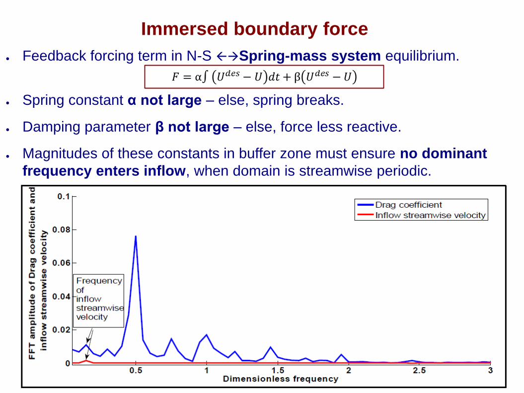
● Feedback forcing term in N-S Spring-mass system equilibrium.

● Spring constant α not large – else, spring breaks.

● Damping parameter β not large – else, force less reactive.

● Magnitudes of these constants in buffer zone must ensure no dominant

frequency enters inflow, when domain is streamwise periodic.

Immersed boundary force

Documents

Presentazione standard di PowerPoint - DICAT