PREVENTING A REPEAT OF THE MONEY MARKET MELTDOWN OF THE EARLY 1930S

JOHN V. DUCA

RESEARCH DEPARTMENT

WORKING PAPER 0904

Federal Reserve Bank of Dallas

Preventing a Repeat of the Money Market Meltdown of the Early 1930s John V. Duca*

Vice President and Senior Policy Advisor Research Department, Federal Reserve Bank of Dallas

P.O. Box 655906, Dallas, TX 75265 (214) 922-5154, john.v.duca@dal.frb.org

and Southern Methodist University, Dallas, TX April 2009 (revised November 2009)

This paper analyzes the meltdown of the commercial paper market during the Great

Depression, and relates those findings to the recent financial crisis. Theoretical models of financial frictions and information problems imply that lenders will make fewer non-collateralized loans or investments and relatively more extensions of collateralized finance in times of high risk premiums. This study investigates the relevance of such theories to the Great Depression by analyzing whether the increased use of a collateralized form of business lending (bankers acceptances) relative to that of non-collateralized commercial paper can be econometrically attributable to measures of corporate credit/financial risk premiums. Because commercial paper and bankers acceptances are short-lived, they are more timely measures of the availability of short-term credit than are bank or business failures and the level or growth rate of the stock of bank loans, whose maturities were often longer and were renegotiable. In this way, the study adds to the literature on financial market frictions during the Great Depression, which aside from analyzing securities prices, typically investigates the behavior of credit-related variables that lag current conditions, such as bank failures, bankruptcies, the stock of money, or outstanding bank loans.

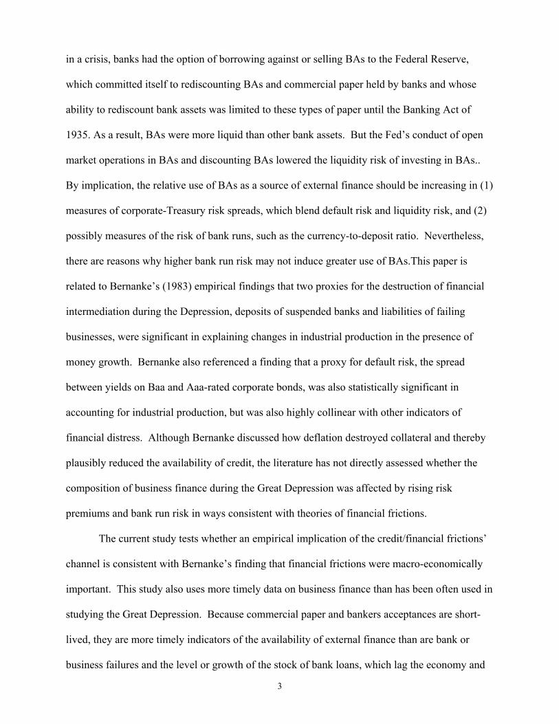
In particular, the real level of bankers acceptances and their use relative to non-collateralized commercial paper were strongly and positively related to spreads between corporate and treasury bond yields. Also significant were short-run events, such as the October 1929 stock market crash and the 1933 bank holiday episode that sparked flights to quality in the bond market and a flight to collateral (BAs) in the money market and perhaps away from the loan market. Furthermore, these shifts in the composition of external finance were large, supporting the view that financial frictions and reduced credit availability may have played an important role in depressing the U.S. economy during the 1930s.

The paper also relates these findings to the current financial crisis by examining how the relative use of commercial paper reacted to yield spreads during the current crisis, taking into account Federal Reserve actions to improve liquidity conditions in the money markets. Results suggest that these efforts may have, at least so far, helped prevent the commercial paper market from melting down to the extent seen during the early 1930s. JEL Classification Codes: E44, E50, N12 *I thank Danielle DiMartino and Gustavo Suarez for suggestions, David Luttrell and Jessica Renier for research assistance, and seminar participants at Oxford University, Johns Hopkins University, the Bank for International Settlements, the 2009 Bank of Canada - Simon Fraser University Conference on Financial Market Stability, the 2008 North American Economics and Finance Association the 2006 Western Economic Association Meeting, the 2007 Swiss Society for Financial Market Research Meeting, and the 2007 Financial Management Association Meeting for comments and suggestions on an earlier, pre-2008 financial crisis version of this paper. The views expressed are those of the author’s and are not necessarily those of the Federal Reserve Bank of Dallas or the Federal Reserve System.

1

This paper analyzes the meltdown of the commercial paper market during the Great

Depression and relates those findings to the recent financial crisis, particularly with respect to

Federal Reserve and Treasury efforts to improve liquidity conditions in the money markets.

Theoretical models of financial frictions imply that credit extensions will shift from risky to safer

borrowers if economic factors increase default risk or increase the cost of loanable funds via

increasing liquidity risk premiums (e.g., Bernanke and Blinder, 1988; Bernanke and

Gertler,1989; Bernanke, Gertler, and Gilchrist, 1996; Jaffee and Russell, 1976; Keeton, 1979;

Lang and Nakamura, 1995; and Stiglitz and Weiss, 1981). Based on these implications, post-

World War II data on the composition of business credit has been used to assess the relevance of

such theories, dating back to at least Jaffee and Modigliani (1969), who assess the composition

of bank business lending, and extending to recent studies, such as Kashyap, Wilcox, and Stein

(1993), who analyze the relative use of commercial paper and bank loans. This literature,

especially the flight-to-quality model of Lang and Nakamura (1995) and the financial accelerator

approach of Bernanke, Gertler, and Gilchrist (1996), implies that lenders will make fewer non-

secured loans and extend relatively more collateralized finance in times of high default risk.

Studies of the current crisis may be hampered by what some may misperceive as a lack of

historical precedent, but the current study provides an analysis of the relative use of commercial

paper during the Great Depression to shed light on how the money markets have been affected

by the current crisis. It also provides evidence that Fed/Treasury efforts may have (so far)

prevented the commercial paper market from imploding on the scale that it did in 1932. In

general, empirical studies of the impact of financial frictions and monetary factors during the

1930s have focused on examining the links between bank failures/loans and economic activity

(Bernanke, 1983; and Calomiris and Mason, 2003), the source and impact of the fall in the

money supply (Boughton and Wicker, 1979; Friedman and Schwartz, 1963; and Hamilton,

1992), the role of nonmonetary factors (Temin, 1976 and 1989), the conduct of monetary policy

2

(Field, 1984; and Wheelock, 1990), the role of unanticipated deflation (Hamilton, 1987), or links

between default risk spreads and economic growth (Bernanke, 1983). Although the credit and

financial frictions’ literature, particularly the financial accelerator work of Bernanke and Gertler

(1989) and Bernanke, Gertler, and Gilchrist (1996), is partly motivated by the Great Depression,

there are no published studies that empirically analyze the composition of business credit

extensions during the era, partly reflecting a lack of data on timely measures of external finance.

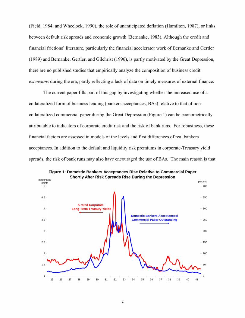
The current paper fills part of this gap by investigating whether the increased use of a

collateralized form of business lending (bankers acceptances, BAs) relative to that of non-

collateralized commercial paper during the Great Depression (Figure 1) can be econometrically

attributable to indicators of corporate credit risk and the risk of bank runs. For robustness, these

financial factors are assessed in models of the levels and first differences of real bankers

acceptances. In addition to the default and liquidity risk premiums in corporate-Treasury yield

spreads, the risk of bank runs may also have encouraged the use of BAs. The main reason is that

 

1

1.5

2

2.5

3

3.5

4

4.5

5

25 26 27 28 29 30 31 32 33 34 35 36 37 38 39 40 410

50

100

150

200

250

300

350

400

Figure 1: Domestic Bankers Acceptances Rise Relative to Commercial PaperShortly After Risk Spreads Rise During the Depression

percentpercentage

points

A-rated Corporate - Long-Term Treasury Yields

Domestic Bankers Acceptances/Commercial Paper Outstanding

3

in a crisis, banks had the option of borrowing against or selling BAs to the Federal Reserve,

which committed itself to rediscounting BAs and commercial paper held by banks and whose

ability to rediscount bank assets was limited to these types of paper until the Banking Act of

1935. As a result, BAs were more liquid than other bank assets. But the Fed’s conduct of open

market operations in BAs and discounting BAs lowered the liquidity risk of investing in BAs..

By implication, the relative use of BAs as a source of external finance should be increasing in (1)

measures of corporate-Treasury risk spreads, which blend default risk and liquidity risk, and (2)

possibly measures of the risk of bank runs, such as the currency-to-deposit ratio. Nevertheless,

there are reasons why higher bank run risk may not induce greater use of BAs.This paper is

related to Bernanke’s (1983) empirical findings that two proxies for the destruction of financial

intermediation during the Depression, deposits of suspended banks and liabilities of failing

businesses, were significant in explaining changes in industrial production in the presence of

money growth. Bernanke also referenced a finding that a proxy for default risk, the spread

between yields on Baa and Aaa-rated corporate bonds, was also statistically significant in

accounting for industrial production, but was also highly collinear with other indicators of

financial distress. Although Bernanke discussed how deflation destroyed collateral and thereby

plausibly reduced the availability of credit, the literature has not directly assessed whether the

composition of business finance during the Great Depression was affected by rising risk

premiums and bank run risk in ways consistent with theories of financial frictions.

The current study tests whether an empirical implication of the credit/financial frictions’

channel is consistent with Bernanke’s finding that financial frictions were macro-economically

important. This study also uses more timely data on business finance than has been often used in

studying the Great Depression. Because commercial paper and bankers acceptances are short-

lived, they are more timely indicators of the availability of external finance than are bank or

business failures and the level or growth of the stock of bank loans, which lag the economy and

4

which have been analyzed in much of the literature on the Great Depression. A particular

problem with analyzing outstanding bank loans is that bankers may have given troubled

borrowers more time to repay loans or delayed writing off loans. As a result, growth in the stock

of bank loans may not give a consistent nor timely indication of the availability of new credit.

Consistent with a financial frictions channel, bankers acceptances—real or relative to

commercial paper—are increasing in the spreads between investment-grade corporate and

Treasury bond yields. Such spreads are used to gauge risk premiums, without breaking them

down into expected default losses and changes in the price of default and liquidity risk. [Temin

(1976) argues that wider corporate quality spreads reflected heightened risk of business failures

rather than tight liquidity conditions.] Because the money market and corporate spread variables

exhibit drift and nonstationarity during the Great Depression era, cointegration techniques are

used. Given the short maturities of bankers acceptances and commercial paper, results imply that

risk premiums persistently affected the composition and availability of external finance.

To relate these findings to the current crisis, this study also analyzes the current crisis.

Owing to the deepening of financial and credit markets, and the Fed’s shift toward conducting

open market operations in Treasury and agency debt, bankers acceptances have become a trivial

source of domestic finance. Instead, the paper-bank loan mix (Kashyap, Wilcox, and Stein,

1997) is modeled to see how the same Baa-Treasury spread used in the Great Depression sample

is related to the composition of short-term business finance in the current crisis. Results suggest

that actions taken since October to improve liquidity in the money markets may have helped

prevent the commercial paper market from imploding by as much as it did in the early 1930s.

This study is organized as follows. Section 2 provides detail about bankers acceptances

and hypotheses about their use during the Great Depression. Section 3 presents the data and

section 4, the empirical results for this era. Section 5 examines whether new Federal Reserve

5

liquidity programs may have prevented the commercial paper market from collapsing. The

conclusion relates the findings for the Great Depression with those on the current crisis.

II. Details and Hypotheses Regarding Bankers Acceptances and Commercial Paper

What Are Bankers Acceptances and What Purposes Do They Serve?

A bankers acceptance is a time draft drawn on a bank to finance the shipment or storage

of goods. A draft is “accepted” when a bank guarantees payment to the holder. This makes the

BA tradeable in securities markets because the issuing bank unconditionally promises payment

to the investor at a specified date regardless of whether the goods-buying firm repays the bank

and because investors usually have better information about the bank than the goods purchaser.

The goods-buying firm essentially receives funding to pay the seller from a bank, which funds

the extension by selling the bankers acceptance. From the perspective of banks guaranteeing

BAs, the goods purchased or held in inventory collateralize the BAs. Thus, extending BAs

entails less default risk than making an unsecured loan to a firm of similar credit quality.

Why Risk Premiums May Affect The Use of Bankers Acceptances

Theories of credit and financial frictions imply that lenders would pressure borrowers for

more collateral, which is relevant for the BA market during an era when firms had fewer

financing options. Goods sellers, for instance, may be reluctant to give trade credit for an

extended period to a geographically distant customer who is unable to pay within the cash

discount period because they have limited access to external finance. In such cases, the seller

may pressure the buyer to pay using funds from a BA issued by the buyer’s bank. The buyer’s

bank may be more willing to issue a BA than an unsecured loan owing to the difference in

collateral or because it has better information about the buyer’s credit quality and can signal this

to BA investors in an incentive-compatible way by guaranteeing (accepting) the BA.

In addition, in the event that the goods-buying firm does not repay, the buyer’s bank may

be more able to repossess the goods financed with a BA using collection processes than the

6

goods-selling firm. However, the extra paper and legal work in creating a BA versus a standard

loan suggests that many borrowers would be better off with a loan unless the bank requires

collateral that the borrower could not provide absent a BA or unless the value of collateral

induces banks to offer loan rates on unsecured loans above those on BAs. These factors imply

that the relative use of BAs increases with macro default risk, while that of commercial paper

would, consistent with the ratios plotted in Figure 1 and real levels shown in Figure 2.1

Why Liquidity Risk May Affect The Use of Bankers Acceptances

Another attractive aspect of BAs was banks’ ability to sell BAs, which made BAs easier

to fund than business loans, for which deposits were needed (Duffield and Summers, 1981). The

BA market was very liquid in the 1920s and 1930s because the Federal Reserve conducted open

market operations in it (Federer, 2003) and Small and Clouse, 2006). For this reason, BA

issuance reduced the impact of the risk of bank deposit runs on the banks’ ability to meet

customer credit needs. An additional funding advantage was that banks were required to hold

reserves against deposits needed to fund loans, but not against BAs that they issued and sold.

Furthermore, even if banks held BAs they issued, BAs were more liquid than loans. Prior

to 1932, only commercial paper and BAs held by banks were eligible as collateral for discount

loans; and it was not until late 1935 that the Federal Reserve allowed some types of loans to

serve as collateral for discount loans. In 1932, Congress granted the Federal Reserve limited

temporary authority to rediscount promissory notes secured to the satisfaction of the Federal

Reserve under the Glass-Steagall Act. The Federal Reserve interpreted this provision as giving it

limited authority to accept government securities as well as commercial paper and BAs as

collateral for discount loans (The New York Clearinghouse Association, 1953, p.76).2 The

1 Asset-backed commercial paper is relatively new. Unlike BAs which are collateralized by re-sellable goods, much “asset-backed” commercial paper is collateralized by paper assets, whose market values have fallen since mid-2007. 2 Likely reflecting this limited change at the Fed, a dummy variable controlling for this limited and temporary authority was insignificant in regressions not shown.

7

 

1

1.5

2

2.5

3

3.5

4

4.5

5

25 26 27 28 29 30 31 32 33 34 35 36 37 38 39 40 410

100

200

300

400

500

600

700

800

900

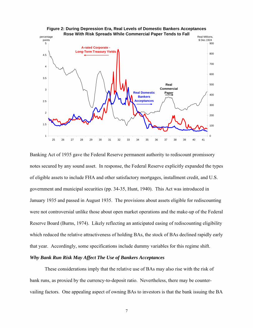
Figure 2: During Depression Era, Real Levels of Domestic Bankers AcceptancesRose With Risk Spreads While Commercial Paper Tends to Fall

Real Millions,$ Dec.1924

percentagepoints

A-rated Corporate - Long-Term Treasury Yields

Real Domestic Bankers

Acceptances

RealCommercial

Paper

Banking Act of 1935 gave the Federal Reserve permanent authority to rediscount promissory

notes secured by any sound asset. In response, the Federal Reserve explicitly expanded the types

of eligible assets to include FHA and other satisfactory mortgages, installment credit, and U.S.

government and municipal securities (pp. 34-35, Hunt, 1940). This Act was introduced in

January 1935 and passed in August 1935. The provisions about assets eligible for rediscounting

were not controversial unlike those about open market operations and the make-up of the Federal

Reserve Board (Burns, 1974). Likely reflecting an anticipated easing of rediscounting eligibility

which reduced the relative attractiveness of holding BAs, the stock of BAs declined rapidly early

that year. Accordingly, some specifications include dummy variables for this regime shift.

Why Bank Run Risk May Affect The Use of Bankers Acceptances

These considerations imply that the relative use of BAs may also rise with the risk of

bank runs, as proxied by the currency-to-deposit ratio. Nevertheless, there may be counter-

vailing factors. One appealing aspect of owning BAs to investors is that the bank issuing the BA

8

guarantees repayment of principal and implied interest regardless of whether the goods-buying

firm repays the issuing bank. That said, confidence in the value of this guarantee may be low

when the risk of bank failures is high. Finally, testing for the impact of bank run risk would be

appropriate if the analysis focused on total BAs. However, in this study detecting any effect may

be difficult because the analysis focuses on BAs that finance domestic commerce—which were

not the bulk of total BAs—to focus on financial frictions effects on domestic borrowing.

Why Liquidity and Bank Run Risk May Also Affect The Use of Commercial Paper

The impact of default and liquidity risk on BA use may have been relevant to the Great

Depression era, when borrower default risk and the liquidity risk posed by bank runs encouraged

banks to shift their portfolios toward less risky assets (Calomiris and Mason, 2004). These types

of risk may have also affected the relative use of commercial paper and bankers acceptances,

both of which are highly liquid and have short-maturities. Since the mid-1970s, un-backed

commercial paper has been issued by firms who pose negligible default risk (in line with

Diamond, 1991). Firms issuing paper are typically required by the market to have back-up lines

of bank credit that eliminate most liquidity risk associated with their ability to pay on time.

For two reasons, however, higher default and liquidity risk during the Great Depression

also plausibly made BAs a more feasible source of external finance than commercial paper.

First, even highly regarded paper issuers posed default risk in that unusual era which preceded

the asset-backed commercial paper market and during which the credit-ratings of many highly

rated firms had been cut by ratings agencies (Wigmore, 1985). Second, it was not until the late

1970s, when large banks had access to well-developed, large time deposit and other funding

markets that paper-issuing firms could easily and normally obtain lines of bank credit to back up

their issuance of paper. Thus, when concerns about liquidity risk rose dramatically, they may

have affected investor perceptions about the liquidity risk of commercial paper during the 1930s.

9

III. Data and Variables

Bankers Acceptances and Commercial Paper

Federal Reserve data are used to construct the ratio of bankers acceptances to commercial

paper (BACP). Both components were seasonally adjusted using a multiplicative X-11

procedure, which yielded a ratio that was similar had the ratio rather than the components been

seasonally adjusted. The advantage of separately adjusting each component is that the same

resulting BA series is used to construct a real BA series that is also modeled. The BA series that

is analyzed excludes BAs used to finance international trade, which are less reflective of

domestic activity and more reflective of swings in international trade that were buffeted by

changes in trade barriers such as the Smoot-Hawley Tariff. A big advantage in using a ratio is

that, in principle, it largely eliminates the need to scale for the level of business activity. Another

advantage is that it generally avoids the need to deflate a nominal level, which entails choosing a

price index from the very limited set of available pre-WWII price indexes. However, the overall

producer price index is used to deflate BA’s and commercial paper to see how each component

behaved and to test for any impact of financial frictions on the real level of BA use. A decline in

real commercial paper and a rise in real BAs were behind the jump in BACP during the early

1930s (Figure 2). This is consistent with a fall in the availability of non-collateralized finance

(e.g., commercial paper) and a surge toward collateralized finance either from former paper

issuers or traditional bank loan borrowers who lost access to unsecured bank loans.

Monthly Federal Reserve data on BAs and commercial paper are available between

December 1924 and December 1941. In 1940-41, there was a large jump in commercial paper,

which plausibly reflected a surge in U.S. production of defense goods purchased by the U.S. and

UK during 1940 and 1941. Because many firms with defense contracts could be viewed as

having both safe revenue sources and even implicit government-backing on their debt obligations

(like commercial paper), the data used in the analysis is restricted to December 1924 to

10

December 1939 to prevent the sample from being contaminated with the omitted variable bias

associated with the ramping up of defense spending in the early 1940s.

Default and Liqiudity Risk

Default and liquidity risk combined are tracked by spreads between yields on investment

grade corporate and long-term U.S. government bonds based on the view that yield spreads

between risky and default free bonds generally reflect cyclical swings in default risk and default

risk premiums (Jaffee, 1975). One such spread is that between yields on A-rated corporate

bonds (Moodys) and long-term U.S. government bonds, denoted as ATR (source: Federal

Reserve (1943), also available from NBER’s Macrohistory Database). ATR was used instead of

the spread between Baa-rated corporate and Treasury bonds (BAATR), which, unlike ATR and

the BA variables, does not have a unit root on a quarterly frequency (upper panel, Table 5) and

exhibits only marginal evidence of a unit root on a monthly basis (upper panel, Table 1).

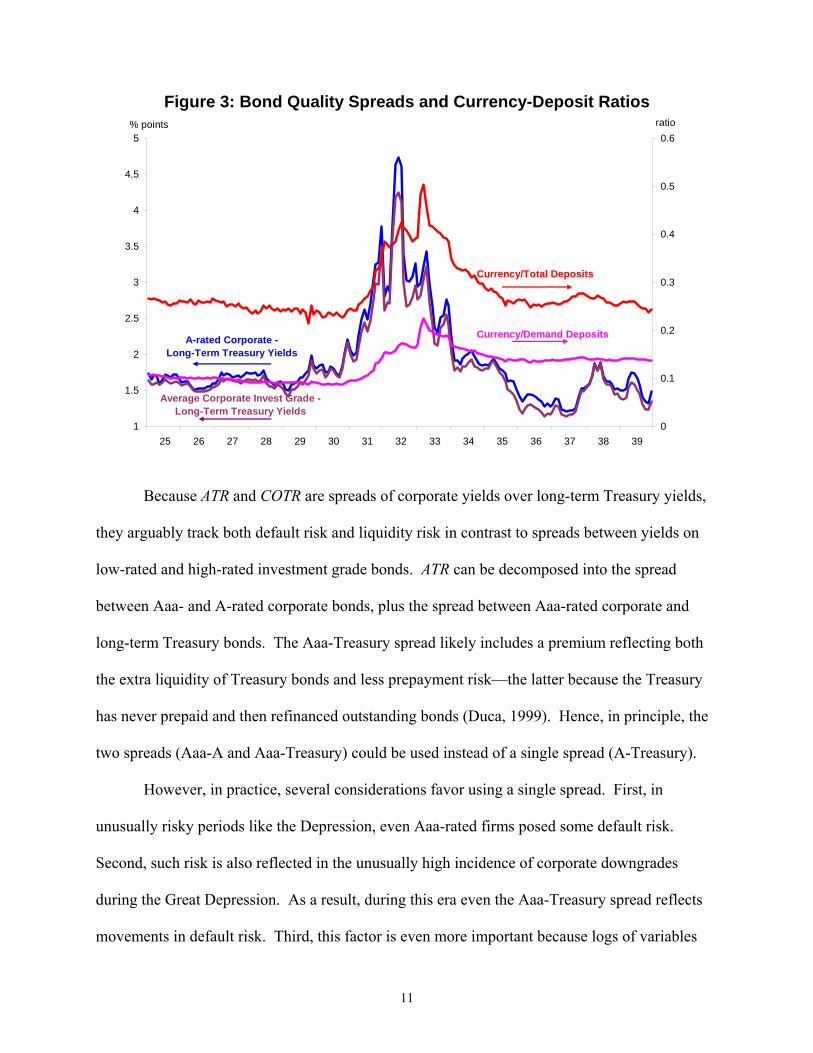
Also used is the spread between average investment grade corporate bond yields and

long-term U.S. government bonds (COTR). Under more “normal” market conditions, there is a

preference in the empirical literature to look at spreads between yields on different ratings

classes of bonds, as such spreads may arguably capture swings in the overall default risk.

However, there were many downgrades of corporate bonds during the Depression in response to

the worsening economy (Wigmore, 1985). This factor suggests that a quality spread based on

the average corporate bond yield might better track changes in default risk than a spread based

on a particular ratings class of bonds. Indeed, the spread between on average investment grade

corporate and long-term Treasury bonds (COTR) somewhat outperforms the spread between

yields on A-rated corporate and long-term U.S. government bonds (ATR). Although they tend to

move closely together, the quality spread based on average corporate yields moved up a little less

than the ATR during the 1931-1932 portion of the Depression era (Figure 3).

11

1

1.5

2

2.5

3

3.5

4

4.5

5

25 26 27 28 29 30 31 32 33 34 35 36 37 38 390

0.1

0.2

0.3

0.4

0.5

0.6

Figure 3: Bond Quality Spreads and Currency-Deposit Ratiosratio% points

A-rated Corporate - Long-Term Treasury Yields

Currency/Total Deposits

Average Corporate Invest Grade - Long-Term Treasury Yields

Currency/Demand Deposits

Because ATR and COTR are spreads of corporate yields over long-term Treasury yields,

they arguably track both default risk and liquidity risk in contrast to spreads between yields on

low-rated and high-rated investment grade bonds. ATR can be decomposed into the spread

between Aaa- and A-rated corporate bonds, plus the spread between Aaa-rated corporate and

long-term Treasury bonds. The Aaa-Treasury spread likely includes a premium reflecting both

the extra liquidity of Treasury bonds and less prepayment risk—the latter because the Treasury

has never prepaid and then refinanced outstanding bonds (Duca, 1999). Hence, in principle, the

two spreads (Aaa-A and Aaa-Treasury) could be used instead of a single spread (A-Treasury).

However, in practice, several considerations favor using a single spread. First, in

unusually risky periods like the Depression, even Aaa-rated firms posed some default risk.

Second, such risk is also reflected in the unusually high incidence of corporate downgrades

during the Great Depression. As a result, during this era even the Aaa-Treasury spread reflects

movements in default risk. Third, this factor is even more important because logs of variables

12

are used, which raises problems arising from Jenson’s inequality associated with decomposing

spreads like ATR and COTR into log subcomponents. Fourth, there is a high degree of

correlation between the Aaa-Treasury and A-Aaa spreads during this era, raising problems of

multi-collinearity—particularly using cointegration techniques on a sample spanning 15 years.

Likely reflecting these considerations, other results (not shown in the tables) which used

components like the logs of the Aaa-Treasury and A-Treasury spreads, gave unusual results.

For three reasons, the analysis uses bond quality spreads rather than interest rate spreads

between BAs and commercial paper. First, the latter may introduce simultaneity bias. Second,

switching to the BA-commercial paper rate spread did not materially affect the key results.

Third, interpreting bond spreads is easier since the BA-commercial paper rate spread may also

reflect relative money market conditions from factors other than default or liquidity risk.

Currency-To-Deposit Ratios

As suggested by much of the monetarist literature (e.g., Friedman and Schwartz, 1963),

ratios of currency held outside of the banking system to bank deposits can be used as indicators

of the risk of bank deposit runs or the public’s lack of confidence in the banking system. Two

such ratios are considered, both constructed with Friedman and Schwartz data that are available

from the NBER. One is the ratio of currency to demand deposits (CDRAT) and the other is the

ratio of currency to demand plus time deposits (CTDRAT). Both are plotted in Figure 3.

Other Financial Crisis or Regulatory Variables

Changes in bank regulation plausibly affected the use of BAs. Two monthly dummies

are used to control for the impact of the Banking Act of 1935. BANKACT359 equals zero before

September 1935 (and one thereafter), when the Banking Act officially took effect. The other,

BANKACT351, equals one since January 1935, when money market participants may have acted

in anticipation of the Act’s passage. These long-term dummy variables did not perform well.

13

This was particularly true with a quarterly dummy, BANKACT35, which equaled 1 from

1935:Q3 on. To conserve space these runs are not shown in the table. Nevertheless, there are

some outsized swings in BACP and the real level of BAs just before and just after the Banking

Act was enacted. As a check to see whether these short-run effects altered the short- and long-

coefficients in quarterly vector-error correction models, a short-run dummy (BACTDD) was

included in some models, which equaled 1 in 1935:q3, negative 1 in 1935:q4, and 0 otherwise.

In addition, some regressions also included a 0-1 variable to account for any temporary,

outsized, impact of the banking crisis of March 1933. The monthly version of this variable,

BANKHOLID, equals one in March 1933, when fears of a banking collapse gripped the U.S.,

inducing President Roosevelt to order a bank holiday. During that shutdown, regulators

examined the books of banks and reopened only the ones deemed solvent ones that month.

Reflecting that the holiday occurred late in March and that the public’s confidence in banks was

still shaken in April, the monthly version of BANKHOLID also equals one in April 1933 and the

quarterly version of this variable equals 1 in 1933:q2 and 0 otherwise. The large jump in relative

BA use without a large jump in default risk spreads during these months strongly suggests that

extreme fears of bank runs at that time induced a flight to collateralized finance.

IV. Empirical Findings

This section presents cointegration tests to assess the relationship between the relative use

of BAs and the two measures of risk on a monthly basis. Then, short-run findings from vector

error-correction models are reviewed. Quarterly results are provided as a robustness check.

Finally, the absolute levels of real BAs are analyzed to see if findings regarding the relative use

of BAs (e.g., BACP) are not merely an artifact of comparing BA use with commercial paper.

4.1 Montlhy Cointegration Results

Cointegration analysis should be used to detect long run relationships among

nonstationary variables (Engle and Granger, 1987), preferably in logs. Since the logs of monthly

14

and quarterly BA use (denoted with an L before BACP) have unit roots (allowing for possible

time trends) as do the default risk spreads LCOTR and ATR, cointegration tests are used to test

for long-run relationships among the relative use of BAs and one default risk spread (LATR or

LCOTR). Each of these variables has a unit root, being nonstationary in levels and stationary in

first differences, according to augmented-Dickey-Fuller statistics that are insignificant for the

levels and significant for the first differences of each variable (upper panel Table 1). Somewhat

stronger results were found using LCOTR, whose results are presented first in Table 1.

Tests found only one cointegrating vector for LBACP and LCOTR for samples including

and excluding observations after the Banking Act of 1935 (vectors 1 and 8) based on two

standard cointegration test statistics (Table 1). One is the trace statistic, which rejected only the

absence of one cointegrating vector in each case at the 5 percent level using Johansen-Juselius’s

(1990) rank significance criterion. The other statistic is the maximum eigenvalue statistic, which

also only rejected the absence of one cointegrating vector in each case at the 5 percent level. In

each case, vectors minimizing the Akaike information statistic favored a lag length of 1 month.

Combined with the insignificant statistics for the existence of more than 1 cointegrating vector

(not shown), these findings support the hypothesis that one long-run (cointegrating) relationship

exists among each group of variables. For the unique estimated vectors 1 and 2, the quality

spread is highly significant with the hypothesized sign, since flipping the coefficient signs in the

cointegrating vector (e.g., LBACP t = 1.798746 + 3.706096*LCOTR t from vector 1) implies that

equilibrium use of BA’s relative to commercial paper is increasing in the spread between yields

on investment grade corporate and long-term Treasury yields. Similar results that support the

financial frictions hypothesis were obtained in vector error-correction models (VECMs, which

jointly estimate long- and short-term relationships) that included BANKHOLIDAY as a short-run

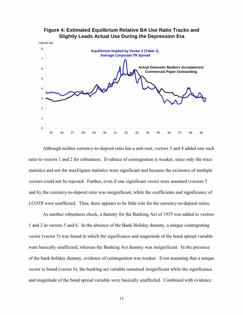
variable (vectors 2 and 8, Table 1). Also encouraging is that actual log levels of BACP are

tracked well and are slightly led by the equilibrium levels implied by vectors 1 and 2 (Figure 4).

15

0

1

2

3

4

5

6

7

8

25 26 27 28 29 30 31 32 33 34 35 36 37 38 39

Figure 4: Estimated Equilbrium Relative BA Use Ratio Tracks andSlightly Leads Actual Use During the Depression Era

natural log

Actual Domestic Bankers Acceptances/Commercial Paper Outstanding

Equilibrium Implied by Vector 2 (Table 1),Average Corporate-TR Spread

Although neither currency-to-deposit ratio has a unit root, vectors 3 and 4 added one such

ratio to vectors 1 and 2 for robustness. Evidence of cointegration is weaker, since only the trace

statistics and not the maxEignen statistics were significant and because the existence of mutliple

vectors could not be rejected. Further, even if one significant vector were assumed (vectors 5

and 6), the currency-to-deposit ratio was insignificant, while the coefficients and significance of

LCOTR were unaffected. Thus, there appears to be little role for the currency-to-deposit ratios.

As another robustness check, a dummy for the Banking Act of 1935 was added to vectors

1 and 2 in vectors 5 and 6. In the absence of the Bank Holiday dummy, a unique cointegrating

vector (vector 5) was found in which the significance and magnitude of the bond spread variable

were basically unaffected, whereas the Banking Act dummy was insignificant. In the presence

of the bank holiday dummy, evidence of cointegration was weaker. Even assuming that a unique

vector is found (vector 6), the banking act variable remained insignificant while the significance

and magnitude of the bond spread variable were basically unaffected. Combined with evidence

16

excluding the 1935-39 sub-period yielded results (vectors 7 and 8) that were similar to those of

vectors 1 and 2, the financial frictions hypothesis is not overturned by controlling for the effects

of the Banking Act of 1935, which appear to be minor and largely insignificant.

All of the above patterns of results are also obtained when the average corporate-

Treasury spread (COTR) was replaced by the A-Treasury bond yield spread (ATR), as can be

seen by comparing models in Table 2 with corresponding models in Table 1.

4.2 Monthly Vector-Error Correction Results

Models of changes in variables whose levels have unit roots and are cointegrated, should

not omit information about long-run relationships to avoid misspecification (Engle and Granger,

1987). In addition to seeing how controlling for short-run effects may alter estimates of long-run

relationships (see Tables 1 and 2), estimating those vector-error correction models (VECM’s),

which jointly estimate long-run and short-run relationships, is helpful in seeing whether the long-

run relationships help explain short-run movements. In estimating short-run movements (first

differences of log-levels), the VECM’s regress the first difference in each long-run variable on

lagged first differences of each long-run factor and include a lagged error-correction (EC) term

equal to actual minus the estimated equilibrium values of the long-run variable modeled. Table 3

presents the short-run models of the relative use of BAs, with the error-correction terms based on

the correspondingly numbered cointegrating vectors in Table 1 that use the spreads between the

average investment grade corporate bond and long-term U.S. government bond yield. Thus, the

even numbered models each include the bank holiday dummy, while other models differ in the

construction of their error-correction term and whether they include an extra t-1 lag first

difference term from adding any additional long-run variable to the cointegrating vector.

Several interesting patterns arise. First, the error-correction term is highly significant,

with the anticipated negative sign. Since the EC term equals actual minus equilibrium use, the

17

negative coefficients imply that the change in actual use will decline if actual use exceeded its

estimated equilibrium level in the prior period. Since the bond spread variable is significant with

the anticipated sign in the long-run relationships, the short-run portions of the VECM’s also

support the financial frictions view that high default risk will induce a greater relative use of

collateralized finance. Second, the sizes of the EC coefficients are reasonable, implying that 3 to

4 percent of disequilibria are eliminated on average each month or roughly 30-40 percent per

year. A third pattern is that the bank holiday variable is highly significant, implying some

additional flight to collateral effect beyond that captured by the bond risk spread, either

implicitly either through the error-correction or the short-run ΔLCOTR term. Fourth, consistent

with the comparisons of vectors 1 and 2 with vectors 7 and 8 in Table 1 (and 2), models 1 and 2

have similar coefficients when the sample excludes the 1935-39 sub-period, as in models 7 and 8

which are placed next to models 1 and 2 in Table 3. This implies that evidence in support of the

financial frictions hypothesis is unaffected by the Banking Act of 1935. Fifth, although the

banking act variable is statistically insignificant in the long-run relationships (in vectors 5 and 6

in Table 1), its first difference is significant in models 5 and 6, suggesting that the Banking Act

of 1935 might have had some short-run effects on the patterns of finance. Sixth, only models 1,

2, 7, and 8, all of which focus solely on a long-run relationship between relative BA use

(LBACP) and the corporate-Treasury yield spread (LCOTR), had residuals that were well

behaved in contrast to other models that tried to include other (statistically insignificant) long-

term factors. Finally, any evidence for short-run effects captured in the currency-to-deposit ratio

is obtained in model 5, but disappears in the presence of the bank holiday variable (model 6).

As a robustness check, similar short-run models from VECM’s that replace the average

corporate bond-Treasury yield spread (LCOTR) with the corporate A-Treasury (LATR) were

estimated. Comparing models in Table 4 with corresponding ones in Table 3 indicates that the

results are qualitatively and quantitatively similar. The only difference is that the models using

18

the average corporate-Treasury yield spread have slightly better fits and more statistically

significant error-correction terms than models using the corporate A-Treasury spread.

4.3 Exogeneity

A natural question is whether the bond yield spreads may be driven by the composition of

the demand for business finance, which would greatly complicate the interpretation of the above

findings. In vector-error correction systems modeling monthly relative BA use, quarterly

relative BA use (analyzed in section 4.4), and quarterly real use of BA’s, the error correction

terms are highly significant in modeling BA use but are highly insignificant in modeling the

corporate-Treasury bond yield spreads, indicating that these yield spreads are weakly exogenous

to BA use. These results point to an asymmetry to how the vector components adjust to

disequilibria, with BA use making the significant adjustments. Thus, consistent with theory, the

equilibrium composition of short-term, external business credit is driven by the combination of

default and liquidity risk measured in the spreads of corporate over Treasury bond yields.

4.4 Quarterly Models of Relative BA Use

Because monthly data are noisy and might obscure long-run patterns, the approach was

repeated using quarterly averages of monthly data. Table 5 and 6 summarize findings that

correspond to the monthly results in Tables 1-4, with three differences. First, Tables 5 and 6

omit results that included a long-run dummy for the Banking Act of 1935 (=1 from 1935:q3-

1939:q4), which were similar to monthly results but were excluded to conserve space.

Nevertheless, some models were tested to control for any short-run effects by including a short-

run dummy, BACTDD, which equals 1 in 1935:q3 and -1 in 1935:q4. Second, because the

number of degrees of freedom is greatly smaller, a sample excluding 1935-1939 was not

presented owing to a very short-sample. Third, a quarterly dummy variable for the stock market

crash of 1929 (STCRASHDD, equals 1 in 1929:q4, -1 in 1930:q1, and 0 otherwise) was included

in some models as a robustness check. By construction, STCRASHDD imposes that any short-

19

run boost to the use of BA’s relative to commercial paper in 1929:q4 is unwound completely in

the first quarter of 1930. Likely reflecting an unwinding that is faster than the normal error-

correction process, this variable outperformed a dummy that equaled 1 in 1929:q4 and 0,

otherwise in regressions not shown. In monthly models not reported, a monthly dummy for the

October 1929 crash was very insignificant, in contrast to the significant quarterly coefficient

found in every model. This difference may reflect that the noisiness of monthly data might

obscure some short-run effects. In fact, virtually all the patterns seen in the monthly results were

obtained in the quarterly models. The notable exception is that the inclusion of controls for the

short-run effects of the bank holiday, the October 1929 stock market crash, and the Banking Act

of 1935 more substantially improves the fit of the short-run models. Nevertheless,

corresponding monthly and quarterly models that omit such short-run variables had similar fits.

The non-stationarity of corporate spreads use over the sample may concern some readers

who are uncomfortable with the notion of a unit root in corporate spreads (note that the currency-

deposit ratios clearly had long-lasting changes in their levels). To allay this concern, one-stage

versions of models 1-3 and 5-7 were run replacing error-correction terms (dated t-1) from

cointegration tests with the t-1 lag levels of relative BA use and corporate spreads. Two quarterly

lags of the first difference of relative BA use and one quarterly lag of the first difference in

corporate spreads are included to control for other short-run dynamic effects. As shown in

Appendix Table A1, the qualitative results are similar. In these models, the significant negative

coefficients on the lag log-level of BA use imply that the gap between the implied long-run

equilibrium and actual BA use is eliminated at quarterly speeds of adjustment of 11-16 percent.

4.5 Quarterly Models of Real BA Use

To see whether these basic results are robust to using absolute rather than relative levels

of BA use, the log level of real BAs (BALEV ) is analyzed with similar variables with a few

adjustments. First, BAs are deflated using the overall wholesale price index (source: NBER

20

Macrohistory Database). Second, reflecting the need for some control for the impact of overall

economic activity on the demand for finance, the NBER index of business activity (BUSACT) is

included in addition to the long-run variables used earlier. As indicated in the upper-panel of

Table 7, the log levels of both variables (denoted with L’s at the start of level variable names)

have unit roots according to augmented Dickey-Fuller statistics. Cointegration tests were first

conducted on vectors (numbers 1 and 5 in Table 7) that included just LBALEV, one spread

variable (LCOTR or LATR), and LBUSACT. Third, also tested were other vectors (numbers 2

and 6, Table 7) that added the bank holiday variable, as well as vectors (numbers 3 and 7) that

added all three short run variables, BANKHOLIDAY, BACTDD, and STCRASH. These are

similar to variables used in analyzing quarterly, relative BA use (BACP) except that the October

1929 stock crash dummy equals 1 in 1929:4 and 0 otherwise. This implicitly assumes less of an

unwinding effect in 1930:q1 than in the stock crash dummy in the BACP models, which also

equaled minus 1 in 1930:q1. Consistent with the differences in the construction of these stock

crash variables was a sharp plunge of commercial paper in 1929:q4 followed by a sharp recovery

in 1930:q1, which would affect LBACP more than LBALEV. Finally, corresponding to vectors 3

and 7 which include all three short-run financial variables, vectors 7 and 8 also include the log of

the currency-to-demand deposit ratio, LCDRATIO, which had a.d.f. statistics closer to exhibiting

a unit root than the currency-to-total deposits ratio (LCTDRATIO). (In other models—not

presented to conserve space—a long-run dummy for the Banking Act of 1935 was insignificant.)

Unique cointegrating relationships were found in each case, with lag lengths of 4 for all

but the two VECMs (vectors 1 and 5) that excluded BANKHOLIDAY, BACTDD, and STCRASH,

in which case 5 lags were needed to find a unique vector. Several patterns emerge from these

vectors in Table 7 and the short-run models in Table 8. First, the quality spread and business

activity variables are statistically significant, with the hypothesized signs, reflecting that BA use

is increasing in the levels of default risk and economic activity. Second, the currency-to-deposit

21

ratio is statistically significant, with a sign indicating that high currency-to-deposit ratios are

associated with lower BA use, ceteris paribus. This result suggests that the negative effects of

investor concerns about the value of bank guarantees on BAs that may have been reflected in the

currency-deposit ratio likely outweighed the positive effects of increased incentives for banks to

issue BAs than make traditional loans. Third, the inclusion of the currency-deposit ratio

increases the magnitude of the coefficient on the quality spread, while reducing that of the

business activity index. Nevertheless, the qualitative results regarding the effects of

liquidity/default risk and business activity on BA use are unaffected by the presence of currency-

deposit ratios. Also noteworthy is how the inclusion of the short-run banking/financial variables

very noticeably improves the fit of the corresponding models, implying that the banking act of

1935 had temporary depressing effects on the real level of BA use, while the stock market crash

and bank holiday episodes induced more use of BA financing, consistent with a flight to

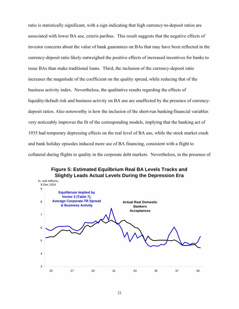
collateral during flights to quality in the corporate debt markets. Nevertheless, in the presence of

   

3

4

5

6

7

8

9

25 27 29 31 33 35 37 39

Figure 5: Estimated Equilbrium Real BA Levels Tracks andSlightly Leads Actual Levels During the Depression Era

ln, real millions,$ Dec.1924

Actual Real Domestic Bankers

Acceptances

Equilibrium Implied byVector 3 (Table 7),

Average Corporate-TR Spread & Business Activity

22

these short-run event controls, the implied long-run equilibrium relationship from quality spreads

and the business activity index track and slightly lead actual log levels of real BAs well (Figure

5). Overall, the findings for the level of real BA use are consistent with those for the use of BAs

relative to commercial paper.

V. Bond Yield Spreads and Business Credit Composition During the Current Crisis

5.1 An Empirical Specification of the Paper-Bank Loan Mix

Since the late 1930s, BAs have become much less important reflecting the deepening of

credit markets and the Fed’s shift to conducting open market operations in Treasuries. This

makes the ratio of BAs to commercial paper less informative. Also, the deepening of the

commercial paper market from the rise of asset-backed paper implies that the links between

commercial paper and real activity are more complicated than during the 1930s. Accordingly,

instead of BACP or the real levels of BAs or commercial paper, we model commercial paper as a

share of commercial paper plus business loans (CPBLMIX, see Kashyap, Wilcox, and Stein,

1997). CPBLIMIX is total commercial paper outstanding (consistently defined since 2001) as a

share of commercial paper and commercial and industrial loans at all commercial banks. It

differs from the mix variable of Kashyap, et al (1997) in including all commercial paper, rather

than just paper issued by nonfinancial corporations. The reason for the difference is the

increasing use during the early part of the decade of credit at many nonfinancial companies who

borrowed financial entities who funded the credit by issuing asset-backed paper. Paper issued

directly by nonfinancial firms declined in relative terms during much of the decade, as did bank

loans, both of which lost market share to asset-backed paper funded credit.

To make the analysis more comparable with that for the Great Depression, CPBLMIX is

modeled as a function of the spread between Baa corporate and 10-year Treasury bond yields

23

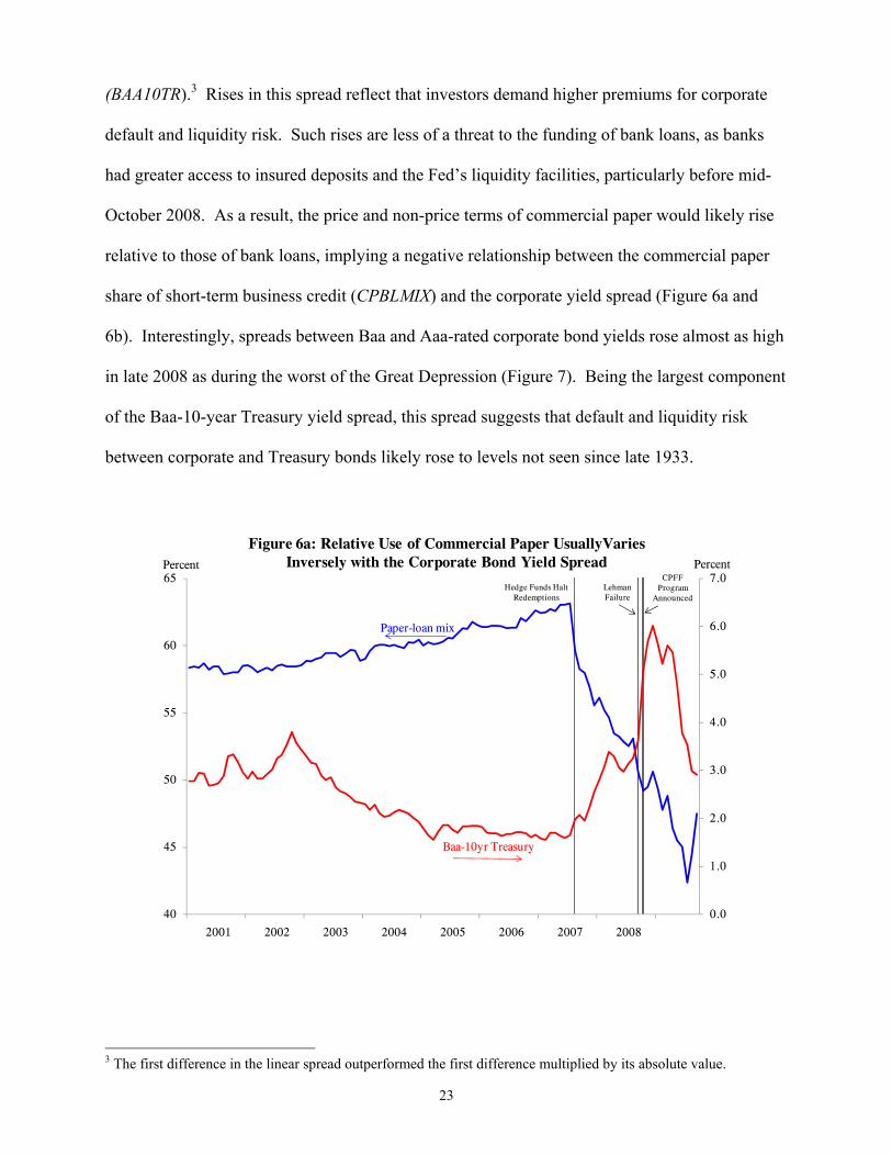
(BAA10TR).3 Rises in this spread reflect that investors demand higher premiums for corporate

default and liquidity risk. Such rises are less of a threat to the funding of bank loans, as banks

had greater access to insured deposits and the Fed’s liquidity facilities, particularly before mid-

October 2008. As a result, the price and non-price terms of commercial paper would likely rise

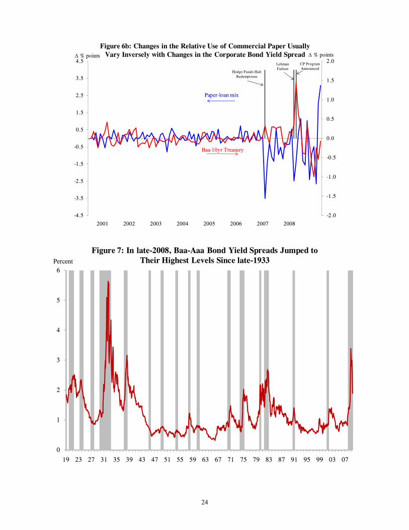
relative to those of bank loans, implying a negative relationship between the commercial paper

share of short-term business credit (CPBLMIX) and the corporate yield spread (Figure 6a and

6b). Interestingly, spreads between Baa and Aaa-rated corporate bond yields rose almost as high

in late 2008 as during the worst of the Great Depression (Figure 7). Being the largest component

of the Baa-10-year Treasury yield spread, this spread suggests that default and liquidity risk

between corporate and Treasury bonds likely rose to levels not seen since late 1933.

0.0

1.0

2.0

3.0

4.0

5.0

6.0

7.0

40

45

50

55

60

65

2001 2002 2003 2004 2005 2006 2007 2008

Figure 6a: Relative Use of Commercial Paper UsuallyVaries Inversely with the Corporate Bond Yield Spread Percent

Baa-10yr Treasury

Paper-loan mix

Percent

Lehman Failure

Hedge Funds Halt Redemptions

CPFF Program

Announced

3 The first difference in the linear spread outperformed the first difference multiplied by its absolute value.

24

-2.0

-1.5

-1.0

-0.5

0.0

0.5

1.0

1.5

2.0

-4.5

-3.5

-2.5

-1.5

-0.5

0.5

1.5

2.5

3.5

4.5

2001 2002 2003 2004 2005 2006 2007 2008

Figure 6b: Changes in the Relative Use of Commercial Paper Usually Vary Inversely with Changes in the Corporate Bond Yield Spread

Baa-10yr Treasury

Paper-loan mix

Δ % pointsLehman Failure

Hedge Funds Halt Redemptions

CP ProgramAnnounced

Δ % points

0

1

2

3

4

5

6

19 23 27 31 35 39 43 47 51 55 59 63 67 71 75 79 83 87 91 95 99 03 07

Figure 7: In late-2008, Baa-Aaa Bond Yield Spreads Jumped to Their Highest Levels Since late-1933Percent

25

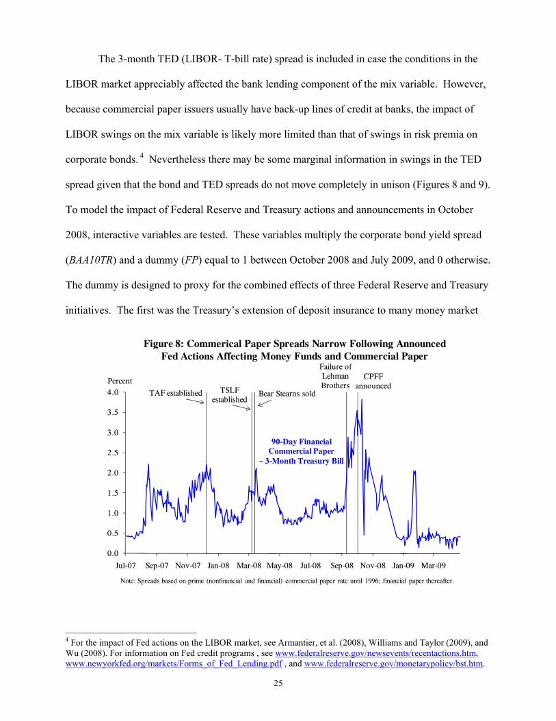
The 3-month TED (LIBOR- T-bill rate) spread is included in case the conditions in the

LIBOR market appreciably affected the bank lending component of the mix variable. However,

because commercial paper issuers usually have back-up lines of credit at banks, the impact of

LIBOR swings on the mix variable is likely more limited than that of swings in risk premia on

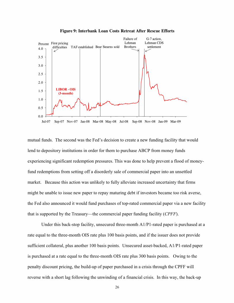
corporate bonds. 4 Nevertheless there may be some marginal information in swings in the TED

spread given that the bond and TED spreads do not move completely in unison (Figures 8 and 9).

To model the impact of Federal Reserve and Treasury actions and announcements in October

2008, interactive variables are tested. These variables multiply the corporate bond yield spread

(BAA10TR) and a dummy (FP) equal to 1 between October 2008 and July 2009, and 0 otherwise.

The dummy is designed to proxy for the combined effects of three Federal Reserve and Treasury

initiatives. The first was the Treasury’s extension of deposit insurance to many money market

0.0

0.5

1.0

1.5

2.0

2.5

3.0

3.5

4.0

Jul-07 Sep-07 Nov-07 Jan-08 Mar-08 May-08 Jul-08 Sep-08 Nov-08 Jan-09 Mar-09

Percent

Figure 8: Commerical Paper Spreads Narrow Following Announced Fed Actions Affecting Money Funds and Commercial Paper

Note: Spreads based on prime (nonfinancial and financial) commercial paper rate until 1996; financial paper thereafter.

TAF established Bear Stearns sold

Failure of Lehman Brothers

CPFF announced

90-Day Financial Commercial Paper

– 3-Month Treasury Bill

TSLF established

4 For the impact of Fed actions on the LIBOR market, see Armantier, et al. (2008), Williams and Taylor (2009), and Wu (2008). For information on Fed credit programs , see www.federalreserve.gov/newsevents/recentactions.htm, www.newyorkfed.org/markets/Forms_of_Fed_Lending.pdf , and www.federalreserve.gov/monetarypolicy/bst.htm.

26

0.0

0.5

1.0

1.5

2.0

2.5

3.0

3.5

4.0

Jul-07 Sep-07 Nov-07 Jan-08 Mar-08 May-08 Jul-08 Sep-08 Nov-08 Jan-09 Mar-09

Percent

Figure 9: Interbank Loan Costs Retreat After Rescue Efforts

TAF established

LIBOR - OIS(3-month)

Bear Stearns sold

Failure of Lehman Brothers

First pricing difficulties

G-7 action, Lehman CDS

settlement

mutual funds. The second was the Fed’s decision to create a new funding facility that would

lend to depository institutions in order for them to purchase ABCP from money funds

experiencing significant redemption pressures. This was done to help prevent a flood of money-

fund redemptions from setting off a disorderly sale of commercial paper into an unsettled

market. Because this action was unlikely to fully alleviate increased uncertainty that firms

might be unable to issue new paper to repay maturing debt if investors became too risk averse,

the Fed also announced it would fund purchases of top-rated commercial paper via a new facility

that is supported by the Treasury—the commercial paper funding facility (CPFF).

Under this back-stop facility, unsecured three-month A1/P1-rated paper is purchased at a

rate equal to the three-month OIS rate plus 100 basis points, and if the issuer does not provide

sufficient collateral, plus another 100 basis points. Unsecured asset-backed, A1/P1-rated paper

is purchased at a rate equal to the three-month OIS rate plus 300 basis points. Owing to the

penalty discount pricing, the build-up of paper purchased in a crisis through the CPFF will

reverse with a short lag following the unwinding of a financial crisis. In this way, the back-up

27

facility created during a period of heightened stress has less marginal effect when crisis

conditions in the paper market return toward normal. To capture this feature, the 0-1 variable

(FP) equals 1 in the months (October 2008 and July 2009) when the Fed held at least 10 percent

of total U.S.-issued commercial paper. In principle, the dummy variable, FP, which equals 1

from October 2008 to July 2009, may also capture other roughly contemporaneous government

interventions, such as the FDIC's Temporary Liquidity Guarantee Program, TARP legislation,

and capital injections. However, the fading of relative use of the CPFF to holding less than 10

percent of outstanding commercial paper in August 2009 is not contemporaneous with the

ending of those programs. Furthermore, the interaction variable loses significance if the

unwinding backstop feature of the CPFF is not taken into account by simply defining FP to equal

one in all months since October 2008, which would better align with the ongoing aspects of

those other facilities. Nevertheless, it is difficult to completely disentangle the effects of these

other facilities.

Reflecting the cushioning effect of such actions on the impact of higher default and

liquidity risk pressures, the interactive term FP *BAA10TR is hypothesized to have an opposite

sign from a non-interactive yield spread. Those hypothesized signs implicitly assume that the

net effect of Fed and Treasury actions to bolster money market conditions and the banking

system had larger short-run cushioning effects on commercial paper market than on bank loans,

which, a priori, is an empirical issue.

Under another liquidity program, the Term Asset-Backed Securities Loan Facility

(TALF) which was started after a long delay in March 2009 (announced in December 2009), the

Fed purchases top-tier rated asset-backed medium-term debt that funds several types of loans,

included business loans backed by the Small Business Administration, equipment loans, credit

cards, student loans, and auto loans. In this program, issuers voluntarily approach the facility for

funding after packaging such securities in accordance with the terms of the program. The start of

28

TALF in March 2009 was accompanied by a revival of commercial paper issuance that later

ebbed in April. Indeed, in all the models March 2009 was a large, positive outlier that largely

unwound in April. Paper issuers and investors may have had miss-placed hopes that the TALF

would help improve liquidity conditions in the commercial paper market for two reasons. First,

reports indicated that markets were apparently disappointed by the low initial volumes of TALF

purchases. Second, and perhaps more importantly, the TALF was designed mainly to improve

liquidity conditions in medium-term asset-backed securities used to fund consumer and business

loans over the medium-, not the very short-run. The liquidity problems arising during the

financial crisis has fostered some segmentation of securities markets (and was a major rationale

for asset market interventions by the Fed and Treasury) that plausibly limited spill-over effects of

the TALF on the commercial paper market. Some models include, ΔTALF, equal to 1 in March

2009, -1 in April, and 0 otherwise. Comparing models 3 with 4 and models 7 with 8, including

ΔTALF cleans up residuals without altering key coefficient estimates other than the TED spread.

To handle unusual event risks that boosted liquidity risk, a dummy variable (Aug14, = 1

in 2007:08, = 0 otherwise) is included for the market reaction to the August 9, 2007 decision by

some European hedge funds to halt redemptions, owing to the lack of market trades on many of

their subprime mortgage-related assets. This induced a surge in LIBOR-OIS and LIBOR-

Treasury spreads that was not immediately picked up by a surge in corporate bond yield spreads

or the t-1 lag of the TED spread. On similar grounds, a dummy for the September 2008 failure

of Lehman (Lehman = 1 in 2008:09, 0 otherwise) is also included. Finally, reflecting that

commercial paper issuance (and hence CPBLMIX) is more dependent on the need to finance

inventories (see Kashyap, Wilcox, and Stein, 1993), regressions also included the log of the

monthly ISM purchasing managers’ (manufacturing) index of inventory demand, which tracks

the change in inventories and is more timely than inventory-shipment ratio data and much less

subject to revisions (LINV). An alternative control for inventories is the 3-month change in the

29

log ISM index (Δ3LINV), where the three-month change reflects the tendency for commercial

paper to have a 3-month maturity. Note that the timing of the ISM survey is early in a month,

and tends to reflect activity in month t-1 (a tendency noted by Harris, 1991). For this reason

simultaneity is not much of an issue since using the time t dated index essentially reflects activity

in period t-1. Furthermore, the index is used as a scaling variable to control for the influence of

inventory swings on the mix variable.

In the short sample over which commercial paper data are consistently defined (2001:01-

2009:09), the paper-mix and bond yield spread variables are I(2),5 reflecting that at the end of the

sample, the paper mix plunges while the bond yield spreads soar, leading to serial correlation in

both levels and first differences at the sample’s end. To limit distortions from such trends, the

models regress first differences of the paper-loan mix on first differences of yield spreads for

months t-1 through t-3 in the presence of control variables (Aug14, Lehman, and LINV/Δ3LINV).

5.2 Empirical Results From Modeling the Paper-Bank Loan Mix During the Crisis

Table 9 presents results from eight regressions that reflect different sample periods and

first difference rate spread variables (Δrspread). Models (1)-(4) use the log-linear ISM inventory

index, while models (5)-(8) instead use the 3-month change in the log of the index, but otherwise

correspond to models (1)-(4) with respect to sample periods and variables. Model 1 covers the

sample through October 2008 and omits any controls for Federal Reserve and Treasury

programs. As hypothesized, the t-1 and t-3 lags of ΔBAATR are negative and significant (the t-2

lag is insignificant), as are the financial crisis dummies (Aug14 and Lehman). However, when

the sample is extended to end in September 2009, the time t-1 lag ΔBAATR is no longer

significant and even has a positive sign. Results are similar in models (5) and (6) using a slightly

5 As per the modified AIC and SIC criteria.

30

different control for inventory activity.6 This shift in coefficients suggests that the new credit

programs may have affected the impact of liquidity and default risk premiums on the relative use

of commercial paper and bank loans.

To shed more light on that hypothesis, models 3, 4, 7, and 8 are estimated over the full

sample and include a 0-1 variable (FP) for the liquidity programs multiplied by the first

difference of the bond yield spread. The inclusion of these terms yields non-interactive rate

spread coefficients that are similar to those in samples ending in October 2008, and interactive

rate spreads (FP*ΔBAATR) that are jointly significant. In particular, the interactive rate spread

coefficients at lags t-1 and t-3 are highly statistically significant and oppositely signed from the

non-interactive rate spreads, consistent with liquidity programs having a desired effect. One

caveat is that March 2009 is a big enough positive outlier, that there is evidence of serial

correlation in the residuals for all the full sample models (2, 3, 6, and 7) that omit the TALF

program variable. This problem appears corrected by the presence of the ΔTALF variable in the

interactive-spread models (4 and 8). The overall patterns of results suggest that the Federal

Reserve and Treasury liquidity programs have helped stabilize the relative use of commercial

paper by counteracting the influence of wider liquidity and default risk premiums. Nevertheless

this interpretation and the findings as a whole should be viewed with caution in light of the short

sample, which makes it infeasible to estimate error-correction models using levels of spreads

with cointegration techniques that may more fully reflect the short- and long-run influences of

securities market conditions on credit flows.

During the early 1930s, the Federal Reserve did not actively intervene in commercial

paper purchases when commercial paper plunged in tandem with rising corporate liquidity and

6 Note that owing to little variation in the inventory diffusion index in the short sample ending in 2008:08, it is difficult to identify an effect of inventories. However, in the longer sample, the inventory variable mainly has a positive and at least marginally statistically significant coefficient, consistent with the general use of commercial paper to finance working capital (such as inventories) and the results of Kashyap, Wilcox, and Stein (1993).

31

default risk premiums, even after it was granted discretion to do so in the summer of 1932 in an

amendment (section 13(3)) of the Federal Reserve Act. In contrast to that episode, the Federal

Reserve has intervened to provide liquidity in the commercial paper market during the current

crisis, especially since October 2008. Although the samples are too short to be definitive, the

evidence thus far supports the working hypothesis that these actions have helped stabilize the use

of commercial paper by countering rising liquidity premiums on corporate debt.

VI. Conclusion

This study analyzes the relative use of a collateralized and easily funded source of

external business finance during the Great Depression and relates those results to money market

conditions during the current financial crisis. Because the forms of finance examined (bankers

acceptances and commercial paper) are short-lived, the timing of their movements should have

been more closely related to contemporaneous changes in default risk spreads than were

bank/firm failures or movements in the stock of bank loans, which lag the economy more and

have been used in prior studies of the Great Depression. The analysis uses spreads on yields

between on A-rated corporate and U.S. Treasury bonds, as well as those between average

investment-grade corporate bonds to track ex ante default and liquidity risk premiums. Also

assessed were currency-to-deposit ratios, which could have risen with liquidity risk pressures on

banks, which would tend to boost BA use or which could have increased with investor doubts

about the value of banks’ backing of BAs, which would lower BA use. Evidence of a net impact

of bank run risk, as proxied by currency-to-deposit ratios, is weak or mixed—with a negative

effect on balance—perhaps reflecting that the ratios may track countervailing factors.

Consistent with Bernanke (1983) and the pre-World War II studies of Kimmel (1939) and

Young (1932), evidence indicates that the provision of credit shifted towards collateralized debt

and debt whose funding sources were less vulnerable to liquidity shocks in reaction to swings in

32

default and possibly liquidity risk during the Great Depression. In particular, the real level of

bankers acceptances and their use relative to non-collateralized commercial paper were strongly

and positively related to bond quality yield spreads. Furthermore, these shifts in the composition

of external finance were large and persistent, supporting the view that financial frictions and

reduced credit availability played an important role in depressing the U.S. economy in the 1930s.

Also significant were short-run events, such as the October 1929 stock market crash and the

1933 bank holiday that sparked flights to quality in the bond market and a flight to quality (BAs)

in the money market and perhaps from the loan market. Overall, the findings from the Great

Depression era are consistent with the implications of research on financial frictions and flights

to quality (e.g., Bernanke and Blinder, 1988; Bernanke and Gertler, 1989; Bernanke, Gertler, and

Gilchrist, 1996; Jaffee and Russell, 1976; Kashyap, Wilcox, and Stein (1993); Keeton, 1979;

Lang and Nakamura, 1995; and Stiglitz and Weiss, 1981).

Those findings are analogous to analyzing the composition of short-term business credit

during the current financial crisis. In particular, up until the Federal Reserve and Treasury

actions of October 2008, when corporate-Treasury bond yield spreads rose, the use of security-

markets funded commercial paper fell relative to bank business loans, which could be funded

with insured deposits. This linkage broke down after the Fed and Treasury’s announcements to

purchase commercial paper, provide discount loans to money market funds, and insure money

market fund accounts. The pre-October 2008 pattern and the ensuing break from it suggest that

the 2008 pullback in commercial paper outstanding owed to spikes in liquidity premiums. This

interpretation is plausible because higher liquidity premiums on the commercial paper are more

amenable to being addressed by the post-September 2008 actions of the Fed and the Treasury,

than are most of solvency questions about commercial paper issuers. Thus far, these actions

appear to have helped prevent an even sharper pullback in commercial paper and helped foster a

reversal of the jump in the commercial paper-Treasury bill spread around the failure of Lehman.

33

Such an interpretation is tentative and preliminary mainly because of the short sample

available for analyzing consistent measures of commercial paper and because the financial crisis

is not yet over. Nevertheless, earlier evidence from the Great Depression era indicates that

security-funded sources of external finance, such as commercial paper, are highly vulnerable to

the jumps in liquidity risk premiums that typically characterize financial crises. Indeed, real

commercial paper outstanding fell 85 percent between July 1930 and May 1933. Furthermore,

recent experience suggests that such surges in liquidity premiums can be countered by

appropriate central bank asset purchases, thereby cushioning the supply of security-funded credit

to high quality borrowers. By means of comparison, real commercial paper fell 74 percent

during the 25 months between July 1930 and August 1932, but by a less dramatic 44 percent in

the 25 months between July 2007 and August 2009. Of course, some of this difference may also

reflect any impact on credit demand and supply of the stronger macroeconomic policy response

in the recent episode. Nevertheless, the impacts of rate spread variables on the relative use of

commercial paper were estimated in the presence of some controls for credit demand in both

periods, and commercial paper volumes began rising during the summer of 2009. In addition,

some of the beneficial effects of the commercial paper funding facility may be hard to

disentangle from complementary effects of other efforts to bolster liquidity in credit markets.

With appropriate caveats, findings from both the Great Depression and the recent financial crisis

suggest that new liquidity programs in the U.S. have, thus far, helped prevent the money markets

from melting down by as fast as they did during the early 1930s.

34

References

Armantier, Olivier, Krieger, Sandra, and McAndrews, James, “The Federal Reserve’s Term Auction

Facility,” Federal Reserve Bank of New York Current Issues in Economics and Finance, vol. 14,

no. 5, July 2008.

Bernanke, Ben S. (1983), “Non-Monetary Effects of Financial Crises in the Propagation of the Great

Depression,” American Economic Review 71, 257-76.

Bernanke, Ben S. and Mark Gertler (1989), “Agency Costs, Net Worth, and Business Fluctuations,”

American Economic Review 79, 14-31.

Bernanke, Ben S., Gertler, Mark, and Simon Gilchrist (1996), “The Financial Accelerator and the Flight

to Quality, Review of Economics and Statistics 58, 1-15.

Board of Governors of the Federal Reserve System (1943), Banking and Monetary Statistics: 1914-41.

Washington, DC: Board of Governors of the Federal Reserve System.

Boughton, James M. and Elmus R. Wicker (1979), “The Behavior of the Currency-Deposit Ratio During

the Great Depression,” Journal of Money, Credit, and Banking 11, 405-18.

Burns, Helen M. (1974), The American Banking Community and New Deal Banking Reforms 1933-35.

Westport, Connecticut: Greenwood Press.

Calomiris, Charles W. and Joseph R. Mason (2003), “Consequences of Bank Distress During the Great

Depression,” American Economic Review 93, 935-47.

Calomiris, Charles W. and Berry Wilson (2004), “Bank Capital and Portfolio Management: The 1930s

“Capital Crunch” and the Scramble to Shed Risk,” Journal of Business 77, 421-55.

Diamond, Douglas W. (1991), “"Monitoring and Reputation: The Choice Between Bank Loans and

Directly Placed Debt," Journal of Political Economy 91, 689-721.

Duca, John V. (1999), "An Overview of What Credit Market Indicators Tell Us," Economic and

Financial Review, Federal Reserve Bank of Dallas, 1999:Q3.

35

Duca, John V., DiMartino, Danielle, and Renier, Jessica (2009), “Fed Confronts Financial Crisis By

Expanding Its Role As Lender of Last Resort,” Federal Reserve Bank of Dallas Economic Letter,

February/March 2009. <http://dallasfed.org/research/eclett/2009/el0902.pdf>

Duca, John V. and Stuart S. Rosenthal (1991), “An Empirical Test of Credit Rationing in the Mortgage

Market,” Journal of Urban Economics 29, 218-34.

Duffield, Jeremy G. and Bruce J. Summers (1981), “Bankers Acceptances,” in Instruments of the Money

Market, edited by Timothy Q. Cook and Bruce J. Summers, pp. 126-35. Richmond, Virginia:

Federal Reserve Bank of Virginia.

Engle, Robert F. and Clive W.J. Granger (1987), “Co-integration and Error Correction: Representation,

Estimation, and Testing,” Econometrica, 55, 251–276.

Federer, J. Peter (2003), “Institutional Innovation and the Creation of Liquid Financial Markets: The

Case of Bankers Acceptances, 1914-34,” Journal of Economic History 63, 666-94.

Field, Alexander J. (1984), “A New Interpretation of the Onset of the Great Depression,” Journal of

Economic History 44, 489-98.

Friedman, Milton and Anna J. Schwartz (1963), A Monetary History of the United States 1867-1960.

Princeton: Princeton University Press.

Friedman, Milton and Anna J. Schwartz (1970), Monetary Statistics of the United States: Estimates,

Sources, Methods. New York: National Bureau of Economic Research.

Gordon, Robert J. and James A. Wilcox (1981), “Monetarist Interpretations of the Great Depression: An

Evaluation and Critique,” in The Great Depression Revisited, edited by Karl Brunner, pp. 49-

107. Boston: Martinus Nijhoff Publishing.

Hamilton, James D. (1987), “Monetary Factors in the Great Depression,” Journal of Monetary

Economics 19, 145-70.

Hamilton, James D. (1992), “Was the Deflation During the Great Depression Anticipated: Evidence

from the Commodity Futures Markets,” American Economic Review 82, 157-78.

36

Harris, Ethan, (1991), "Tracking the Economy with the Purchasing Managers' Index." Federal Reserve

Bank of New York Quarterly Review 16, no. 3, 61-69.

Jaffee, Dwight M., and Franco Modigliani (1969), “A Theory and Test of Credit Rationing,” American

Economic Review 59, 850-72.

Jaffee, Dwight M. (1975), “Cyclical Variations in the Risk Structure of Interest Rates,” Journal of

Monetary Economics 1, 309-25.

Jaffee, Dwight M. and Thomas Russell (1976), “Imperfect Information, Uncertainty, and Credit

Rationing,” Quarterly Journal of Economics 90, 651-66.

Kashyap, Anil, Wilcox, David E, and Jeremy Stein (1993), “Monetary Policy and Credit Conditions:

Evidence from the Composition of External Finance,” American Economic Review 83, 78-98.

Keeton, William R. (1979), Equilibrium Credit Rationing, New York: Garland.

Kimmel, Lewis H. (1939), The Availability of Bank Credit 1933-38. New York: National Industrial

Conference Board.

Lang, William W., and Nakamura, Leonard I. (1995), " 'Flight to Quality' in Bank Lending and

Economic Activity," with William W. Lang, Journal of Monetary Economics 36, 145-64.

NBER Macrohistory Database. < http://www.nber.org/databases/macrohistory>.

Small, David H. and Clouse, James (2005), “The Scope of Monetary Policy Actions Authorized Under

the Federal Reserve Act,” The Berkeley Journals in Macroeconomics 5, Issue 1, Article 6, <

<http://www.bepress.com/cgi/viewcontent.cgi?article=1255&context=bejm> .

Stiglitz, Joseph E. and Andrew Weiss (1981), “Credit Rationing in Markets with Imperfect

Information,” American Economic Review 71, 393-410.

Temin, Peter (1976), Did Monetary Forces Cause the Great Depression? New York: W. W. Norton.

Temin, Peter (1989), Lessons From the Great Depression. Cambridge, Massachusetts: The MIT Press.

Wheelock, David C. (1990), “Member Bank Borrowing and the Fed’s Contractionary Monetary Policy

during the Great Depression,” Journal of Money, Credit, and Banking 22, 409-26.

37

Wigmore, Barrie A. (1985), The Crash and Its Aftermath: 1929-1933. Westport, Connecticut:

Greenwood Press.

Williams, John C., and Taylor, John B. (2009), “A Black Swan in the Money Market,” American

Economic Journal: Macroeconomics, vol. 1, no. 1, 58–83.

Wu, Tao (2008), “On the Effectiveness of the Federal Reserve’s New Liquidity Facilities,” Federal

Reserve Bank of Dallas, Working Paper no. 0808, May 2008.

Young, Ralph A. (1932), The Availability of Bank Credit. New York: National Industrial Conference

Board.

38

Available Upon Request, Not Intended for Publication

Appendix A: How This Paper’s Study of the Great Depression Relates to the 2007 Turmoil in Asset-Backed Commercial Paper Markets

Compared to the current menu of corporate finance, financial markets were much less

developed during the era examined. Partly to offset liquidity risk to investors, commercial paper

issuers are forced by market forces to obtain formal back-up lines of bank credit to ensure timely

payment, a practice which generally began in the 1970s.

However, default risk remains an important aspect facing securities markets. Ostensibly

to address such concerns and to expand the availability of commercial paper, the asset-backed

commercial paper (ABCP) market had grown rapidly and by yearend 2006, provided slightly

more finance than more traditional commercial paper. Many of the assets backing commercial

paper were securities, including now-suspect subprime mortgage instruments. As unanticipated

increases in problem subprime mortgages mounted, the value of the assets backing this paper

became highly suspect in the summer of 2007. Ironically, it was asset-backed commercial paper

that was hardest hit, probably because the paper had been viewed as safe based on the financial

assets serving as collateral rather than the underlying strength of the issuing firm as in the case of

traditional nonfinancial commercial paper. Nevertheless, this event is consistent with this

study’s findings from the 1930s. For much of the recent crisis, little paper ineligible for the

CPFF was issued, ostensibly because investors viewed such paper as lacking in liquidity or

sufficient collateral backing. In contrast, during the 1930s the liquidity of the BA market was

sustained by the Fed’s conduct of money market operations and BAs were (and still are) backed

by more concrete and re-sellable commodities and products. In this regard, the evidence

presented in this study provides insights about how and why surges in liquidity and default risk

that may result in flights to quality that sometimes affect the commercial paper market.

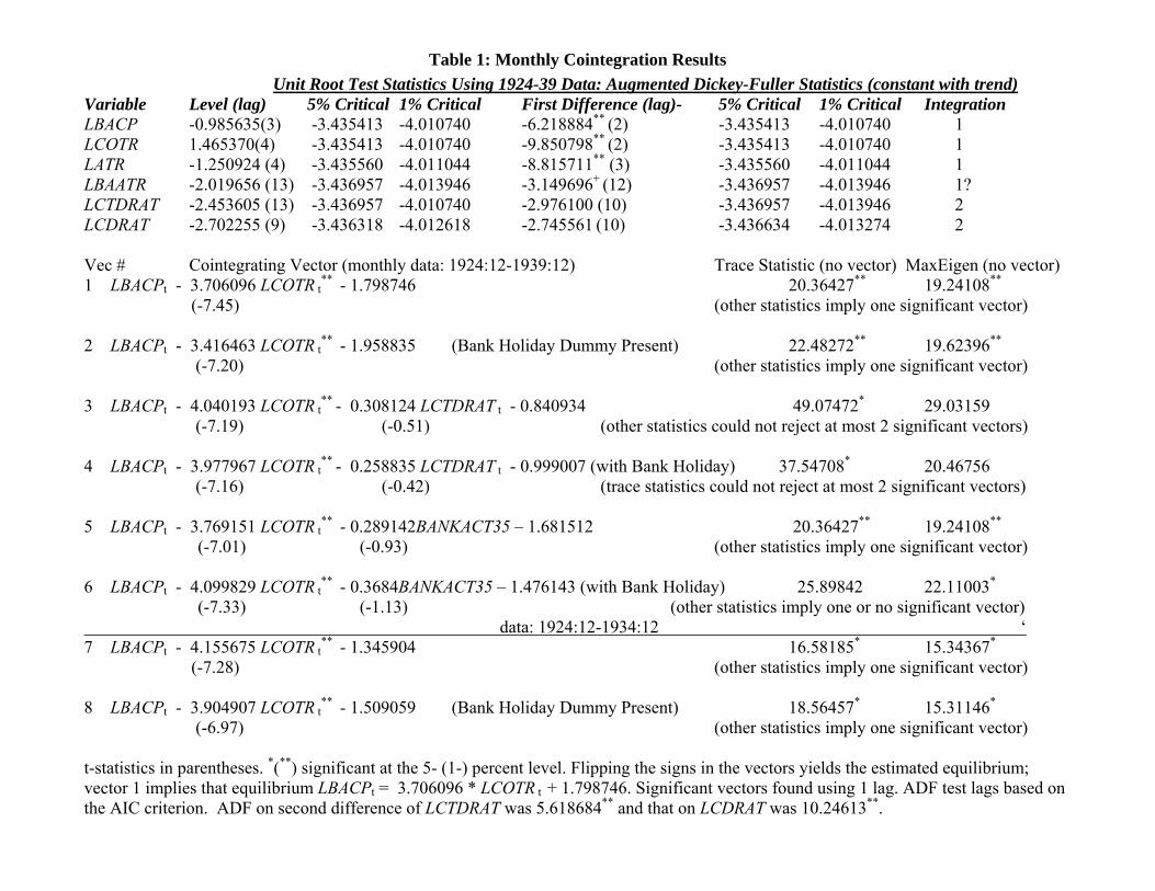
Table 1: Monthly Cointegration Results Unit Root Test Statistics Using 1924-39 Data: Augmented Dickey-Fuller Statistics (constant with trend)

Variable Level (lag) 5% Critical 1% Critical First Difference (lag)- 5% Critical 1% Critical Integration LBACP -0.985635(3) -3.435413 -4.010740 -6.218884** (2) -3.435413 -4.010740 1 LCOTR 1.465370(4) -3.435413 -4.010740 -9.850798** (2) -3.435413 -4.010740 1 LATR -1.250924 (4) -3.435560 -4.011044 -8.815711** (3) -3.435560 -4.011044 1 LBAATR -2.019656 (13) -3.436957 -4.013946 -3.149696+ (12) -3.436957 -4.013946 1? LCTDRAT -2.453605 (13) -3.436957 -4.010740 -2.976100 (10) -3.436957 -4.013946 2 LCDRAT -2.702255 (9) -3.436318 -4.012618 -2.745561 (10) -3.436634 -4.013274 2 Vec # Cointegrating Vector (monthly data: 1924:12-1939:12) Trace Statistic (no vector) MaxEigen (no vector) 1 LBACPt - 3.706096 LCOTR t

** - 1.798746 20.36427** 19.24108** (-7.45) (other statistics imply one significant vector)

2 LBACPt - 3.416463 LCOTR t

** - 1.958835 (Bank Holiday Dummy Present) 22.48272** 19.62396** (-7.20) (other statistics imply one significant vector)

3 LBACPt - 4.040193 LCOTR t** - 0.308124 LCTDRAT t - 0.840934 49.07472* 29.03159

(-7.19) (-0.51) (other statistics could not reject at most 2 significant vectors) 4 LBACPt - 3.977967 LCOTR t

** - 0.258835 LCTDRAT t - 0.999007 (with Bank Holiday) 37.54708* 20.46756

(-7.16) (-0.42) (trace statistics could not reject at most 2 significant vectors) 5 LBACPt - 3.769151 LCOTR t

** - 0.289142BANKACT35 – 1.681512 20.36427** 19.24108** (-7.01) (-0.93) (other statistics imply one significant vector) 6 LBACPt - 4.099829 LCOTR t

** - 0.3684BANKACT35 – 1.476143 (with Bank Holiday) 25.89842 22.11003* (-7.33) (-1.13) (other statistics imply one or no significant vector) data: 1924:12-1934:12 ‘ 7 LBACPt - 4.155675 LCOTR t

** - 1.345904 16.58185* 15.34367* (-7.28) (other statistics imply one significant vector)

8 LBACPt - 3.904907 LCOTR t

** - 1.509059 (Bank Holiday Dummy Present) 18.56457* 15.31146* (-6.97) (other statistics imply one significant vector)

t-statistics in parentheses. *(**) significant at the 5- (1-) percent level. Flipping the signs in the vectors yields the estimated equilibrium; vector 1 implies that equilibrium LBACPt = 3.706096 * LCOTR t

+ 1.798746. Significant vectors found using 1 lag. ADF test lags based on the AIC criterion. ADF on second difference of LCTDRAT was 5.618684** and that on LCDRAT was 10.24613**.

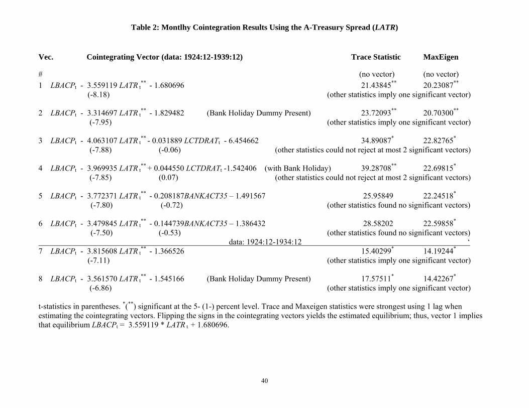
40

Table 2: Montlhy Cointegration Results Using the A-Treasury Spread (LATR) Vec. Cointegrating Vector (data: 1924:12-1939:12) Trace Statistic MaxEigen

# (no vector) (no vector) 1 LBACPt - 3.559119 LATR t

** - 1.680696 21.43845** 20.23087** (-8.18) (other statistics imply one significant vector)

2 LBACPt - 3.314697 LATR t

** - 1.829482 (Bank Holiday Dummy Present) 23.72093** 20.70300** (-7.95) (other statistics imply one significant vector)

3 LBACPt - 4.063107 LATR t** - 0.031889 LCTDRATt - 6.454662 34.89087* 22.82765*

(-7.88) (-0.06) (other statistics could not reject at most 2 significant vectors) 4 LBACPt - 3.969935 LATR t

** + 0.044550 LCTDRATt -1.542406 (with Bank Holiday) 39.28708** 22.69815*

(-7.85) (0.07) (other statistics could not reject at most 2 significant vectors) 5 LBACPt - 3.772371 LATR t

** - 0.208187BANKACT35 – 1.491567 25.95849 22.24518*

(-7.80) (-0.72) (other statistics found no significant vectors) 6 LBACPt - 3.479845 LATR t

** - 0.144739BANKACT35 – 1.386432 28.58202 22.59858* (-7.50) (-0.53) (other statistics found no significant vectors) data: 1924:12-1934:12 ‘ 7 LBACPt - 3.815608 LATR t

** - 1.366526 15.40299* 14.19244* (-7.11) (other statistics imply one significant vector)

8 LBACPt - 3.561570 LATR t

** - 1.545166 (Bank Holiday Dummy Present) 17.57511* 14.42267* (-6.86) (other statistics imply one significant vector)

t-statistics in parentheses. *(**) significant at the 5- (1-) percent level. Trace and Maxeigen statistics were strongest using 1 lag when estimating the cointegrating vectors. Flipping the signs in the cointegrating vectors yields the estimated equilibrium; thus, vector 1 implies that equilibrium LBACPt = 3.559119 * LATR t

+ 1.680696.

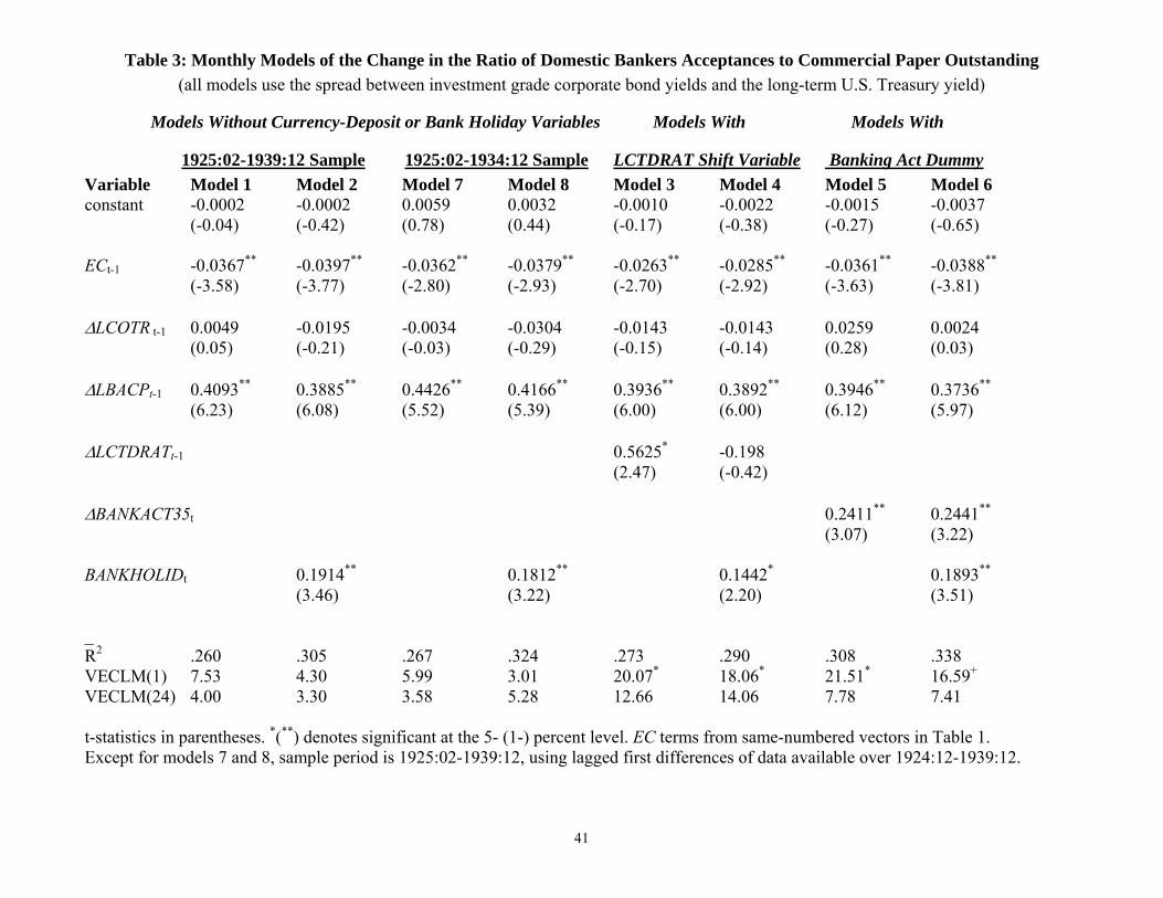
41

Table 3: Monthly Models of the Change in the Ratio of Domestic Bankers Acceptances to Commercial Paper Outstanding (all models use the spread between investment grade corporate bond yields and the long-term U.S. Treasury yield)

Models Without Currency-Deposit or Bank Holiday Variables Models With Models With

1925:02-1939:12 Sample 1925:02-1934:12 Sample LCTDRAT Shift Variable Banking Act Dummy Variable Model 1 Model 2 Model 7 Model 8 Model 3 Model 4 Model 5 Model 6 constant -0.0002 -0.0002 0.0059 0.0032 -0.0010 -0.0022 -0.0015 -0.0037 (-0.04) (-0.42) (0.78) (0.44) (-0.17) (-0.38) (-0.27) (-0.65) ECt-1 -0.0367** -0.0397** -0.0362** -0.0379** -0.0263** -0.0285** -0.0361** -0.0388** (-3.58) (-3.77) (-2.80) (-2.93) (-2.70) (-2.92) (-3.63) (-3.81) ΔLCOTR t-1 0.0049 -0.0195 -0.0034 -0.0304 -0.0143 -0.0143 0.0259 0.0024 (0.05) (-0.21) (-0.03) (-0.29) (-0.15) (-0.14) (0.28) (0.03) ΔLBACPt-1 0.4093** 0.3885** 0.4426** 0.4166** 0.3936** 0.3892** 0.3946** 0.3736**

(6.23) (6.08) (5.52) (5.39) (6.00) (6.00) (6.12) (5.97) ΔLCTDRATt-1 0.5625* -0.198 (2.47) (-0.42) ΔBANKACT35t 0.2411** 0.2441**

(3.07) (3.22) BANKHOLIDt 0.1914** 0.1812** 0.1442* 0.1893**

(3.46) (3.22) (2.20) (3.51) _ R2 .260 .305 .267 .324 .273 .290 .308 .338 VECLM(1) 7.53 4.30 5.99 3.01 20.07* 18.06* 21.51* 16.59+ VECLM(24) 4.00 3.30 3.58 5.28 12.66 14.06 7.78 7.41 t-statistics in parentheses. *(**) denotes significant at the 5- (1-) percent level. EC terms from same-numbered vectors in Table 1. Except for models 7 and 8, sample period is 1925:02-1939:12, using lagged first differences of data available over 1924:12-1939:12.

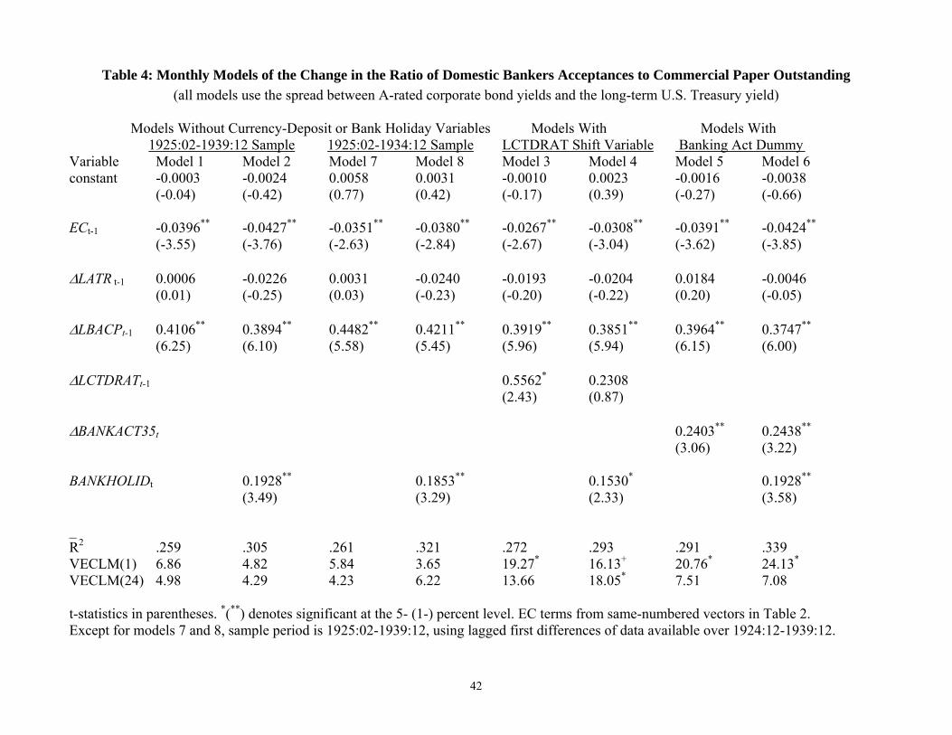
42

Table 4: Monthly Models of the Change in the Ratio of Domestic Bankers Acceptances to Commercial Paper Outstanding (all models use the spread between A-rated corporate bond yields and the long-term U.S. Treasury yield)

Models Without Currency-Deposit or Bank Holiday Variables Models With Models With

1925:02-1939:12 Sample 1925:02-1934:12 Sample LCTDRAT Shift Variable Banking Act Dummy Variable Model 1 Model 2 Model 7 Model 8 Model 3 Model 4 Model 5 Model 6 constant -0.0003 -0.0024 0.0058 0.0031 -0.0010 0.0023 -0.0016 -0.0038 (-0.04) (-0.42) (0.77) (0.42) (-0.17) (0.39) (-0.27) (-0.66) ECt-1 -0.0396** -0.0427** -0.0351** -0.0380** -0.0267** -0.0308** -0.0391** -0.0424** (-3.55) (-3.76) (-2.63) (-2.84) (-2.67) (-3.04) (-3.62) (-3.85) ΔLATR t-1 0.0006 -0.0226 0.0031 -0.0240 -0.0193 -0.0204 0.0184 -0.0046 (0.01) (-0.25) (0.03) (-0.23) (-0.20) (-0.22) (0.20) (-0.05) ΔLBACPt-1 0.4106** 0.3894** 0.4482** 0.4211** 0.3919** 0.3851** 0.3964** 0.3747**

(6.25) (6.10) (5.58) (5.45) (5.96) (5.94) (6.15) (6.00) ΔLCTDRATt-1 0.5562* 0.2308 (2.43) (0.87) ΔBANKACT35t 0.2403** 0.2438**

(3.06) (3.22) BANKHOLIDt 0.1928** 0.1853** 0.1530* 0.1928**

(3.49) (3.29) (2.33) (3.58) _ R2 .259 .305 .261 .321 .272 .293 .291 .339 VECLM(1) 6.86 4.82 5.84 3.65 19.27* 16.13+ 20.76* 24.13* VECLM(24) 4.98 4.29 4.23 6.22 13.66 18.05* 7.51 7.08 t-statistics in parentheses. *(**) denotes significant at the 5- (1-) percent level. EC terms from same-numbered vectors in Table 2. Except for models 7 and 8, sample period is 1925:02-1939:12, using lagged first differences of data available over 1924:12-1939:12.

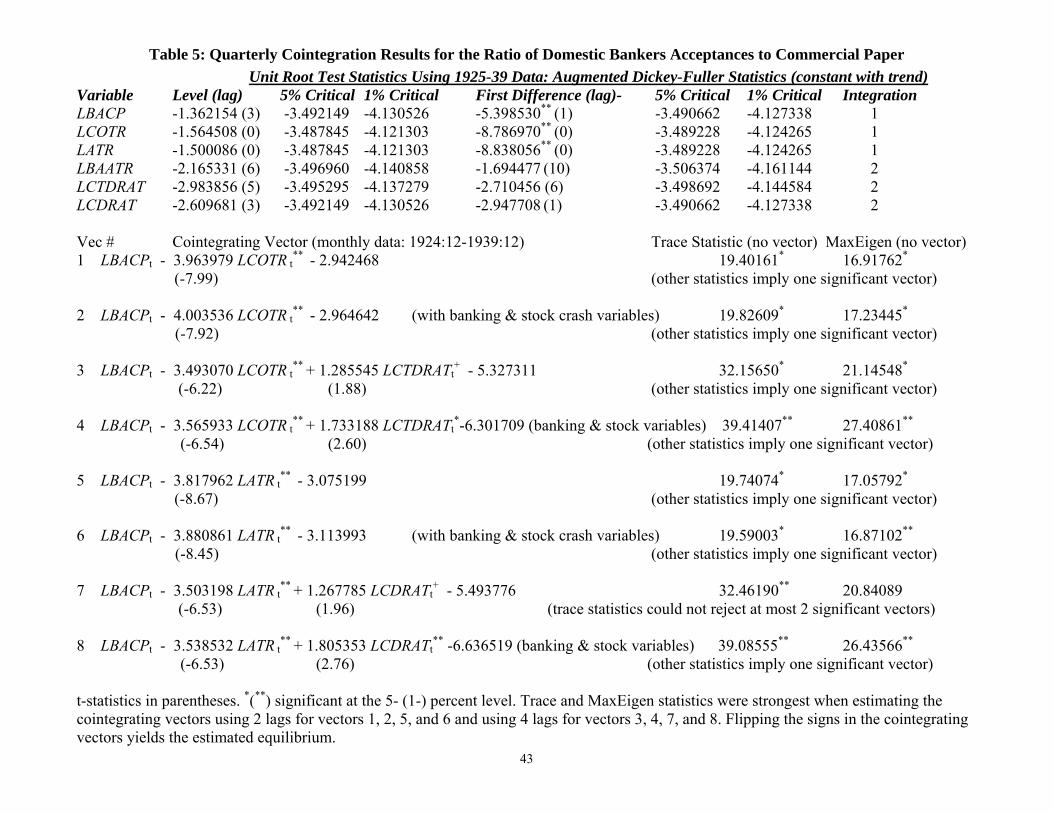
43

Table 5: Quarterly Cointegration Results for the Ratio of Domestic Bankers Acceptances to Commercial Paper Unit Root Test Statistics Using 1925-39 Data: Augmented Dickey-Fuller Statistics (constant with trend)

Variable Level (lag) 5% Critical 1% Critical First Difference (lag)- 5% Critical 1% Critical Integration LBACP -1.362154 (3) -3.492149 -4.130526 -5.398530** (1) -3.490662 -4.127338 1 LCOTR -1.564508 (0) -3.487845 -4.121303 -8.786970** (0) -3.489228 -4.124265 1 LATR -1.500086 (0) -3.487845 -4.121303 -8.838056** (0) -3.489228 -4.124265 1 LBAATR -2.165331 (6) -3.496960 -4.140858 -1.694477 (10) -3.506374 -4.161144 2 LCTDRAT -2.983856 (5) -3.495295 -4.137279 -2.710456 (6) -3.498692 -4.144584 2 LCDRAT -2.609681 (3) -3.492149 -4.130526 -2.947708 (1) -3.490662 -4.127338 2 Vec # Cointegrating Vector (monthly data: 1924:12-1939:12) Trace Statistic (no vector) MaxEigen (no vector) 1 LBACPt - 3.963979 LCOTR t

** - 2.942468 19.40161* 16.91762* (-7.99) (other statistics imply one significant vector)

2 LBACPt - 4.003536 LCOTR t

** - 2.964642 (with banking & stock crash variables) 19.82609* 17.23445*

(-7.92) (other statistics imply one significant vector)

3 LBACPt - 3.493070 LCOTR t** + 1.285545 LCTDRATt

+ - 5.327311 32.15650* 21.14548*

(-6.22) (1.88) (other statistics imply one significant vector) 4 LBACPt - 3.565933 LCOTR t

** + 1.733188 LCTDRATt*-6.301709 (banking & stock variables) 39.41407** 27.40861**

(-6.54) (2.60) (other statistics imply one significant vector) 5 LBACPt - 3.817962 LATR t

** - 3.075199 19.74074* 17.05792* (-8.67) (other statistics imply one significant vector)

6 LBACPt - 3.880861 LATR t

** - 3.113993 (with banking & stock crash variables) 19.59003* 16.87102**

(-8.45) (other statistics imply one significant vector)

7 LBACPt - 3.503198 LATR t** + 1.267785 LCDRATt

+ - 5.493776 32.46190** 20.84089

(-6.53) (1.96) (trace statistics could not reject at most 2 significant vectors) 8 LBACPt - 3.538532 LATR t

** + 1.805353 LCDRATt** -6.636519 (banking & stock variables) 39.08555** 26.43566**

(-6.53) (2.76) (other statistics imply one significant vector) t-statistics in parentheses. *(**) significant at the 5- (1-) percent level. Trace and MaxEigen statistics were strongest when estimating the cointegrating vectors using 2 lags for vectors 1, 2, 5, and 6 and using 4 lags for vectors 3, 4, 7, and 8. Flipping the signs in the cointegrating vectors yields the estimated equilibrium.

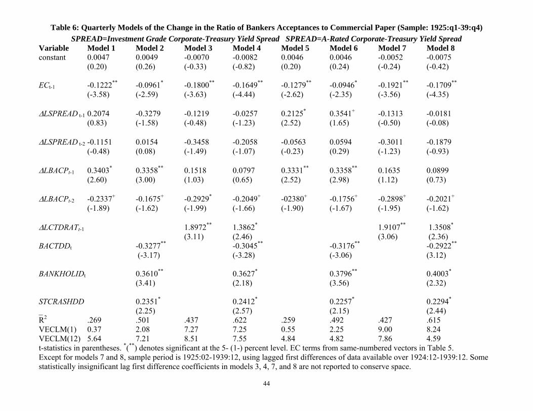
44

Table 6: Quarterly Models of the Change in the Ratio of Bankers Acceptances to Commercial Paper (Sample: 1925:q1-39:q4) SPREAD=Investment Grade Corporate-Treasury Yield Spread SPREAD=A-Rated Corporate-Treasury Yield Spread Variable Model 1 Model 2 Model 3 Model 4 Model 5 Model 6 Model 7 Model 8 constant 0.0047 0.0049 -0.0070 -0.0082 0.0046 0.0046 -0.0052 -0.0075 (0.20) (0.26) (-0.33) (-0.82) (0.20) (0.24) (-0.24) (-0.42) ECt-1 -0.1222** -0.0961* -0.1800** -0.1649** -0.1279** -0.0946* -0.1921** -0.1709** (-3.58) (-2.59) (-3.63) (-4.44) (-2.62) (-2.35) (-3.56) (-4.35) ΔLSPREAD t-1 0.2074 -0.3279 -0.1219 -0.0257 0.2125* 0.3541+ -0.1313 -0.0181 (0.83) (-1.58) (-0.48) (-1.23) (2.52) (1.65) (-0.50) (-0.08) ΔLSPREAD t-2 -0.1151 0.0154 -0.3458 -0.2058 -0.0563 0.0594 -0.3011 -0.1879 (-0.48) (0.08) (-1.49) (-1.07) (-0.23) (0.29) (-1.23) (-0.93) ΔLBACPt-1 0.3403* 0.3358** 0.1518 0.0797 0.3331** 0.3358** 0.1635 0.0899

(2.60) (3.00) (1.03) (0.65) (2.52) (2.98) (1.12) (0.73) ΔLBACPt-2 -0.2337+ -0.1675+ -0.2929* -0.2049+ -02380+ -0.1756+ -0.2898+ -0.2021+

(-1.89) (-1.62) (-1.99) (-1.66) (-1.90) (-1.67) (-1.95) (-1.62) ΔLCTDRATt-1 1.8972** 1.3862* 1.9107** 1.3508* (3.11) (2.46) (3.06) (2.36) BACTDDt -0.3277** -0.3045** -0.3176** -0.2922**

(-3.17) (-3.28) (-3.06) (3.12) BANKHOLIDt 0.3610** 0.3627* 0.3796** 0.4003*

(3.41) (2.18) (3.56) (2.32) STCRASHDD 0.2351* 0.2412* 0.2257* 0.2294* _ (2.25) (2.57) (2.15) (2.44) R2 .269 .501 .437 .622 .259 .492 .427 .615 VECLM(1) 0.37 2.08 7.27 7.25 0.55 2.25 9.00 8.24 VECLM(12) 5.64 7.21 8.51 7.55 4.84 4.82 7.86 4.59 t-statistics in parentheses. *(**) denotes significant at the 5- (1-) percent level. EC terms from same-numbered vectors in Table 5. Except for models 7 and 8, sample period is 1925:02-1939:12, using lagged first differences of data available over 1924:12-1939:12. Some statistically insignificant lag first difference coefficients in models 3, 4, 7, and 8 are not reported to conserve space.

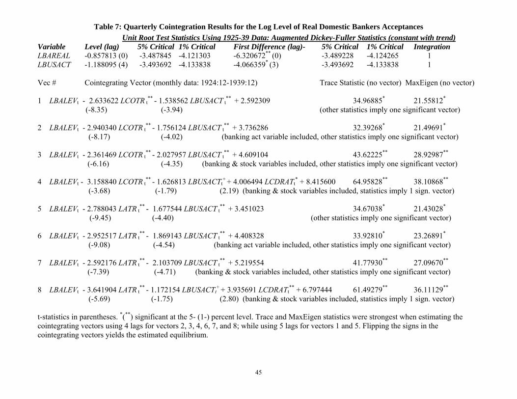
45

Table 7: Quarterly Cointegration Results for the Log Level of Real Domestic Bankers Acceptances Unit Root Test Statistics Using 1925-39 Data: Augmented Dickey-Fuller Statistics (constant with trend)

Variable Level (lag) 5% Critical 1% Critical First Difference (lag)- 5% Critical 1% Critical Integration LBAREAL -0.857813 (0) -3.487845 -4.121303 -6.320672** (0) -3.489228 -4.124265 1 LBUSACT -1.188095 (4) -3.493692 -4.133838 -4.066359* (3) -3.493692 -4.133838 1 Vec # Cointegrating Vector (monthly data: 1924:12-1939:12) Trace Statistic (no vector) MaxEigen (no vector) 1 LBALEVt - 2.633622 LCOTR t

** - 1.538562 LBUSACT t** + 2.592309 34.96885* 21.55812*

(-8.35) (-3.94) (other statistics imply one significant vector)

2 LBALEVt - 2.940340 LCOTR t** - 1.756124 LBUSACT t

** + 3.736286 32.39268* 21.49691* (-8.17) (-4.02) (banking act variable included, other statistics imply one significant vector)

3 LBALEVt - 2.361469 LCOTR t

** - 2.027957 LBUSACT t** + 4.609104 43.62225** 28.92987**

(-6.16) (-4.35) (banking & stock variables included, other statistics imply one significant vector) 4 LBALEVt - 3.158840 LCOTR t

** - 1.626813 LBUSACTt+ + 4.006494 LCDRATt

* + 8.415600 64.95828** 38.10868** (-3.68) (-1.79) (2.19) (banking & stock variables included, statistics imply 1 sign. vector) 5 LBALEVt - 2.788043 LATR t

** - 1.677544 LBUSACT t** + 3.451023 34.67038* 21.43028*

(-9.45) (-4.40) (other statistics imply one significant vector)

6 LBALEVt - 2.952517 LATR t** - 1.869143 LBUSACT t

** + 4.408328 33.92810* 23.26891* (-9.08) (-4.54) (banking act variable included, other statistics imply one significant vector)

7 LBALEVt - 2.592176 LATR t

** - 2.103709 LBUSACT t** + 5.219554 41.77930** 27.09670**

(-7.39) (-4.71) (banking & stock variables included, other statistics imply one significant vector) 8 LBALEVt - 3.641904 LATR t

** - 1.172154 LBUSACTt+ + 3.935691 LCDRATt

** + 6.797444 61.49279** 36.11129** (-5.69) (-1.75) (2.80) (banking & stock variables included, statistics imply 1 sign. vector) t-statistics in parentheses. *(**) significant at the 5- (1-) percent level. Trace and MaxEigen statistics were strongest when estimating the cointegrating vectors using 4 lags for vectors 2, 3, 4, 6, 7, and 8; while using 5 lags for vectors 1 and 5. Flipping the signs in the cointegrating vectors yields the estimated equilibrium.

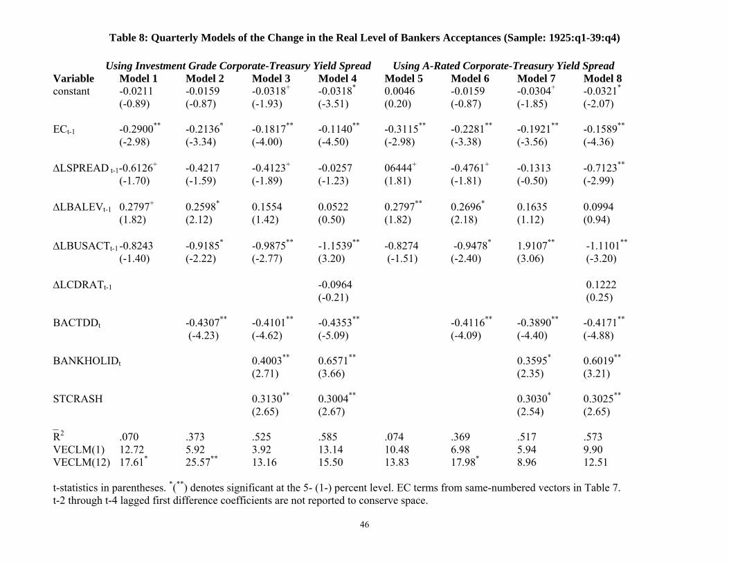
46

Table 8: Quarterly Models of the Change in the Real Level of Bankers Acceptances (Sample: 1925:q1-39:q4) Using Investment Grade Corporate-Treasury Yield Spread Using A-Rated Corporate-Treasury Yield Spread Variable Model 1 Model 2 Model 3 Model 4 Model 5 Model 6 Model 7 Model 8 constant -0.0211 -0.0159 -0.0318+ -0.0318* 0.0046 -0.0159 -0.0304+ -0.0321* (-0.89) (-0.87) (-1.93) (-3.51) (0.20) (-0.87) (-1.85) (-2.07) ECt-1 -0.2900** -0.2136* -0.1817** -0.1140** -0.3115** -0.2281** -0.1921** -0.1589** (-2.98) (-3.34) (-4.00) (-4.50) (-2.98) (-3.38) (-3.56) (-4.36) ΔLSPREAD t-1-0.6126+ -0.4217 -0.4123+ -0.0257 06444+ -0.4761+ -0.1313 -0.7123** (-1.70) (-1.59) (-1.89) (-1.23) (1.81) (-1.81) (-0.50) (-2.99) ΔLBALEVt-1 0.2797+ 0.2598* 0.1554 0.0522 0.2797** 0.2696* 0.1635 0.0994

(1.82) (2.12) (1.42) (0.50) (1.82) (2.18) (1.12) (0.94) ΔLBUSACTt-1 -0.8243 -0.9185* -0.9875** -1.1539** -0.8274 -0.9478* 1.9107** -1.1101** (-1.40) (-2.22) (-2.77) (3.20) (-1.51) (-2.40) (3.06) (-3.20) ΔLCDRATt-1 -0.0964 0.1222 (-0.21) (0.25) BACTDDt -0.4307** -0.4101** -0.4353** -0.4116** -0.3890** -0.4171**

(-4.23) (-4.62) (-5.09) (-4.09) (-4.40) (-4.88) BANKHOLIDt 0.4003** 0.6571** 0.3595* 0.6019**

(2.71) (3.66) (2.35) (3.21) STCRASH 0.3130** 0.3004** 0.3030* 0.3025** (2.65) (2.67) (2.54) (2.65) _ R2 .070 .373 .525 .585 .074 .369 .517 .573 VECLM(1) 12.72 5.92 3.92 13.14 10.48 6.98 5.94 9.90 VECLM(12) 17.61* 25.57** 13.16 15.50 13.83 17.98* 8.96 12.51 t-statistics in parentheses. *(**) denotes significant at the 5- (1-) percent level. EC terms from same-numbered vectors in Table 7. t-2 through t-4 lagged first difference coefficients are not reported to conserve space.

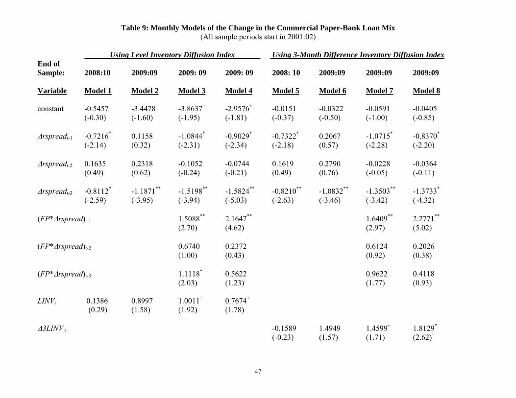
47

Table 9: Monthly Models of the Change in the Commercial Paper-Bank Loan Mix

(All sample periods start in 2001:02) Using Level Inventory Diffusion Index Using 3-Month Difference Inventory Diffusion Index End of Sample: 2008:10 2009:09 2009: 09 2009: 09 2008: 10 2009:09 2009:09 2009:09 Variable Model 1 Model 2 Model 3 Model 4 Model 5 Model 6 Model 7 Model 8 constant -0.5457 -3.4478 -3.8637+ -2.9576+ -0.0151 -0.0322 -0.0591 -0.0405 (-0.30) (-1.60) (-1.95) (-1.81) (-0.37) (-0.50) (-1.00) (-0.85) Δrspreadt-1 -0.7216* 0.1158 -1.0844* -0.9029* -0.7322* 0.2067 -1.0715* -0.8370* (-2.14) (0.32) (-2.31) (-2.34) (-2.18) (0.57) (-2.28) (-2.20) Δrspreadt-2 0.1635 0.2318 -0.1052 -0.0744 0.1619 0.2790 -0.0228 -0.0364 (0.49) (0.62) (-0.24) (-0.21) (0.49) (0.76) (-0.05) (-0.11) Δrspreadt-3 -0.8112* -1.1871** -1.5198** -1.5824** -0.8210** -1.0832** -1.3503** -1.3733* (-2.59) (-3.95) (-3.94) (-5.03) (-2.63) (-3.46) (-3.42) (-4.32) (FP*Δrspread)t-1 1.5088** 2.1647** 1.6409** 2.2771** (2.70) (4.62) (2.97) (5.02) (FP*Δrspread)t-2 0.6740 0.2372 0.6124 0.2026 (1.00) (0.43) (0.92) (0.38) (FP*Δrspread)t-3 1.1118* 0.5622 0.9622+ 0.4118 (2.03) (1.23) (1.77) (0.93) LINVt 0.1386 0.8997 1.0011+ 0.7674+

(0.29) (1.58) (1.92) (1.78) Δ3LINV t -0.1589 1.4949 1.4599+ 1.8129*

(-0.23) (1.57) (1.71) (2.62)

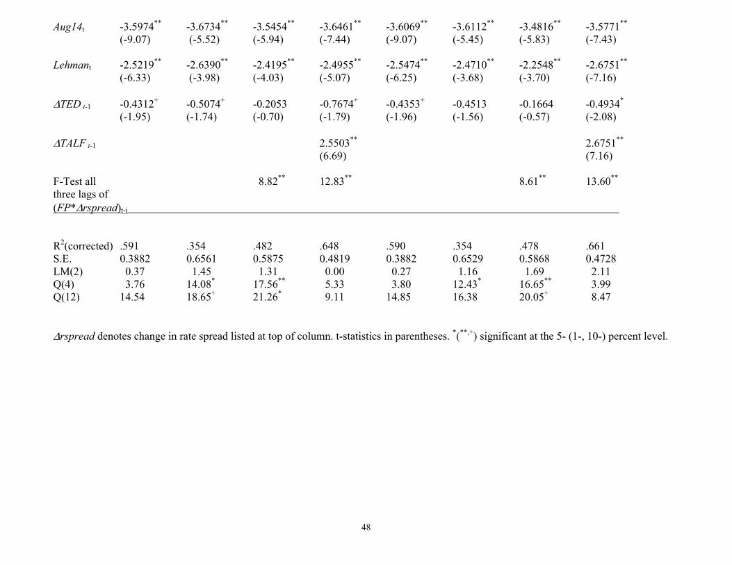
48

Aug14t -3.5974** -3.6734** -3.5454** -3.6461** -3.6069** -3.6112** -3.4816** -3.5771**

(-9.07) (-5.52) (-5.94) (-7.44) (-9.07) (-5.45) (-5.83) (-7.43) Lehmant -2.5219** -2.6390** -2.4195** -2.4955** -2.5474** -2.4710** -2.2548** -2.6751**

(-6.33) (-3.98) (-4.03) (-5.07) (-6.25) (-3.68) (-3.70) (-7.16) ΔTED t-1 -0.4312+ -0.5074+ -0.2053 -0.7674+ -0.4353+ -0.4513 -0.1664 -0.4934*

(-1.95) (-1.74) (-0.70) (-1.79) (-1.96) (-1.56) (-0.57) (-2.08) ΔTALF t-1 2.5503**

2.6751** (6.69) (7.16) F-Test all 8.82** 12.83** 8.61** 13.60** three lags of (FP*Δrspread)t-i R2(corrected) .591 .354 .482 .648 .590 .354 .478 .661 S.E. 0.3882 0.6561 0.5875 0.4819 0.3882 0.6529 0.5868 0.4728 LM(2) 0.37 1.45 1.31 0.00 0.27 1.16 1.69 2.11 Q(4) 3.76 14.08* 17.56** 5.33 3.80 12.43* 16.65** 3.99 Q(12) 14.54 18.65+ 21.26* 9.11 14.85 16.38 20.05+ 8.47 Δrspread denotes change in rate spread listed at top of column. t-statistics in parentheses. *(**,+) significant at the 5- (1-, 10-) percent level.

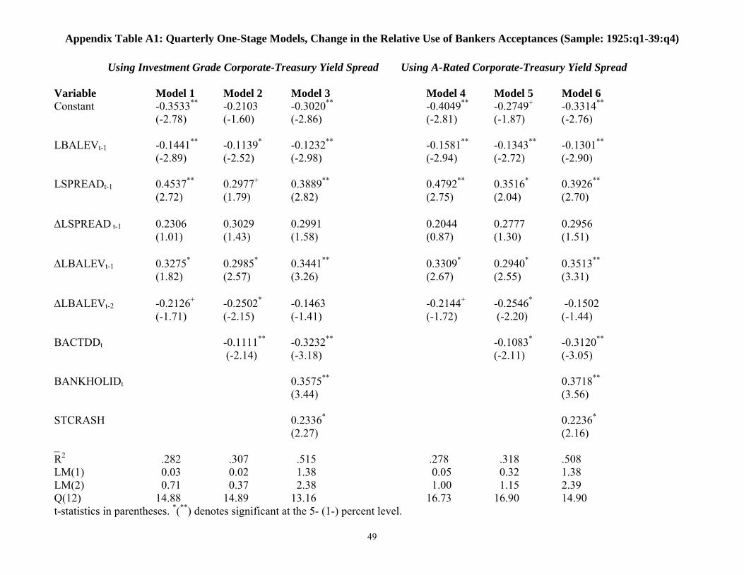
49

Appendix Table A1: Quarterly One-Stage Models, Change in the Relative Use of Bankers Acceptances (Sample: 1925:q1-39:q4) Using Investment Grade Corporate-Treasury Yield Spread Using A-Rated Corporate-Treasury Yield Spread Variable Model 1 Model 2 Model 3 Model 4 Model 5 Model 6 Constant -0.3533** -0.2103 -0.3020** -0.4049** -0.2749+ -0.3314** (-2.78) (-1.60) (-2.86) (-2.81) (-1.87) (-2.76) LBALEVt-1 -0.1441** -0.1139* -0.1232** -0.1581** -0.1343** -0.1301** (-2.89) (-2.52) (-2.98) (-2.94) (-2.72) (-2.90) LSPREADt-1 0.4537** 0.2977+ 0.3889** 0.4792** 0.3516* 0.3926**

(2.72) (1.79) (2.82) (2.75) (2.04) (2.70) ΔLSPREAD t-1 0.2306 0.3029 0.2991 0.2044 0.2777 0.2956

(1.01) (1.43) (1.58) (0.87) (1.30) (1.51) ΔLBALEVt-1 0.3275* 0.2985* 0.3441** 0.3309* 0.2940* 0.3513**

(1.82) (2.57) (3.26) (2.67) (2.55) (3.31) ΔLBALEVt-2 -0.2126+ -0.2502* -0.1463 -0.2144+ -0.2546* -0.1502 (-1.71) (-2.15) (-1.41) (-1.72) (-2.20) (-1.44) BACTDDt -0.1111** -0.3232** -0.1083* -0.3120**

(-2.14) (-3.18) (-2.11) (-3.05) BANKHOLIDt 0.3575** 0.3718**

(3.44) (3.56) STCRASH 0.2336* 0.2236* (2.27) (2.16) _ R2 .282 .307 .515 .278 .318 .508 LM(1) 0.03 0.02 1.38 0.05 0.32 1.38 LM(2) 0.71 0.37 2.38 1.00 1.15 2.39 Q(12) 14.88 14.89 13.16 16.73 16.90 14.90 t-statistics in parentheses. *(**) denotes significant at the 5- (1-) percent level.