Embed Size (px)
Citation preview
Preventives Versus Treatments Redux: Tighter Boundson Distortions in Innovation Incentiveswith an Application to the Global Demand for HIVPharmaceuticals
Michael Kremer1 • Christopher M. Snyder2
� Springer Science+Business Media, LLC, part of Springer Nature 2018
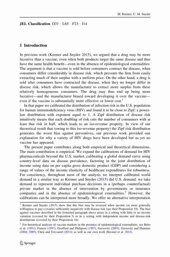
Abstract Kremer and Snyder (Q J Econ 130:1167–1239, 2015) show that demand
curves for a preventive and treatment may have different shapes though they target
the same disease, biasing the pharmaceutical manufacturer toward developing the
lucrative rather than the socially desirable product. This paper tightens the theo-
retical bounds on the potential deadweight loss from such biases. Using a calibration
of the global demand for HIV pharmaceuticals, we demonstrate the dramatically
sharper analysis achievable with the new bounds, allowing us to pinpoint potential
deadweight loss at 62% of the global gain from curing HIV. We use the calibration
to perform policy counterfactuals, assessing welfare effects of government policies
such as a subsidy, reference pricing, and price-discrimination ban. The fit of our
calibration is good: we find that a hypothetical drug monopolist would price an HIV
drug so high that only 4% of the infected population worldwide would purchase,
matching actual drug prices and quantities in the early 2000s before subsidies in
low-income countries ramped up.
Keywords Pharmaceuticals � Deadweight loss � Product development
Electronic supplementary material The online version of this article (https://doi.org/10.1007/s11151-
018-9621-4) contains supplementary material, which is available to authorized users.
& Christopher M. Snyder
Michael Kremer
1 Department of Economics, Harvard University, Littauer Center 207, Cambridge, MA 02138,
USA
2 Department of Economics, Dartmouth College, 301 Rockefeller Hall, Hanover, NH 03755,
USA
123
Rev Ind Organ
https://doi.org/10.1007/s11151-018-9621-4
JEL Classification O31 � L65 � F23 � I14
1 Introduction
In previous work (Kremer and Snyder 2015), we argued that a drug may be more
lucrative than a vaccine, even when both products target the same disease and thus
have the same health benefit—even in the absence of epidemiological externalities.
The argument is that a vaccine is sold before consumers contract the disease, when
consumers differ considerably in disease risk, which prevents the firm from easily
extracting much of their surplus with a uniform price. On the other hand, a drug is
sold after consumers have contracted the disease, when they no longer differ in
disease risk, which allows the manufacturer to extract more surplus from these
relatively homogeneous consumers. The drug may thus end up being more
lucrative—and the manufacturer biased toward developing it over the vaccine—
even if the vaccine is substantially more effective or lower cost.1
In that paper we calibrated the distribution of infection risk in the U.S. population
for human immunodeficiency virus (HIV) and found it to be close to Zipf: a power-
law distribution with exponent equal to 1. A Zipf distribution of disease risk
intuitively means that each doubling of risk cuts the number of consumers with at
least that risk in half, which leads to an iso-revenue property. In view of our
theoretical result that (owing to this iso-revenue property) the Zipf risk distribution
generates the worst bias against preventives, our previous work provided one
explanation for why a variety of HIV drugs have been developed but as yet no
vaccine has appeared.
The present paper contributes along both empirical and theoretical dimensions.
The main contribution is empirical. We expand the calibrations of demand for HIV
pharmaceuticals beyond the U.S. market, calibrating a global demand curve using
country-level data on disease prevalence, factoring in the joint distribution of
income using data on per capita gross domestic product (GDP) and considering a
range of values of the income elasticity of healthcare expenditures for robustness.
For consistency, throughout most of the analysis we interpret calibrated world
demand in a similar way as Kremer and Snyder (2015) did U.S. demand: we take
demand to represent individual purchase decisions in a (perhaps counterfactual)
private market in the absence of intervention by governments or insurance
companies and in the absence of epidemiological externalities.2 However, the
calibrations can be interpreted more broadly. We offer an alternative interpretation
1 Kremer and Snyder (2015) show that this bias may be reversed when income (or more generally
willingness to pay) covaries sufficiently negatively with disease risk (see their Proposition 18). The bias
against vaccines described in the footnoted paragraph above arises in a setting with little or no income
variation (covered by their Proposition 3) or in a setting with independent income and disease-risk
distributions (covered by their Proposition 16).2 For theoretical analyses of vaccine markets in the presence of epidemiological externalities, see Brito
et al. (1991), Francis (1997), Geoffard and Philipson (1997), Gersovitz (2003), Gersovitz and Hammer
(2004; 2005), Chen and Toxvaerd (2014); as well as our own work (Kremer et al. 2012).
M. Kremer, C. M. Snyder
123
of world demand as reflecting purchases by national agencies on behalf of citizens
in their health systems. This interpretation allows for consumer heterogeneity and
epidemiological externalities within countries.
The resulting calibrated demands are employed to examine a range of policy
issues: one exercise leverages Kremer and Snyder’s (2015) formulas for worst-case
bounds on deadweight loss from pharmaceutical sales in the private market. Since
the greatest conceivable distortions occur at the extensive margin (whether a
product is developed at all) rather than the intensive margin (how high the mark up
is for an existing product, which generates a Harberger (1954) deadweight-loss
triangle), the formulas hinge on the percentage of the surplus generated by
completely relieving the disease burden that the producer can extract for itself; we
refer to this as the producer-surplus ratio, denoted q.
The producer-surplus ratio in turn depends on how the demand curve is shaped.
Using the calibrated demands, we can compute q for a monopoly producer of either
a vaccine (v) or a drug (d). In our baseline calibration (indicated by superscript 0),
we obtain a producer-surplus ratio of q0v ¼ 44% for an HIV vaccine. Considering
the market for an HIV vaccine in isolation, we compute a worst-case bound on
deadweight loss of 100 � 44 ¼ 56%. In other words, the distorted incentives
provided by the private market to the firm with regard to the vaccine’s development
and price could dissipate as much as 56% of the global benefit from curing HIV.
Considering the market for an HIV drug in isolation, we compute a baseline
estimate of the drug-producer-surplus ratio of q0d ¼ 38%, which leads to a worst-
case bound on deadweight loss of 100 � 38 ¼ 62%.
Rather than consider the vaccine and drug markets in isolation, it is natural to
wonder what the worst-case deadweight loss is in the comprehensive case in which
either or both products can be produced. The previous theoretical result relevant to
this comprehensive case is Proposition 15 of Kremer and Snyder (2015). We have
been able to tighten the bounds, as reported in Proposition 3 of this paper. For
canonical values of model parameters, these tighter bounds lead to an exact
expression for worst-case deadweight loss as reported in Proposition 2 of this paper.
The exact expression simply equals the larger of the two worst-case bounds for the
isolated products; using the numbers from the calibration, maxð56; 62Þ ¼ 62%. The
previous result merely told us that worst-case deadweight loss in the comprehensive
case is no less than the difference between the worst cases for the individual
products: no less than 62 � 56 ¼ 6%. The new bound thus represents a dramatic
sharpening of the analysis in this application: instead of saying that worst-case
deadweight loss lies somewhere in the interval [6, 100%], we can now pinpoint it at
62%.
The fit of our demand calibration appears to be good. Based on the calibrated
global demand for an HIV drug, we calculate that—in the absence of international
price discrimination, subsidies in low-income countries, or regulatory threats to
intellectual property—a profit-maximizing monopolist would charge such a high
drug price that only about 4% of infected individuals worldwide would buy the
treatment. These price and quantity estimates are remarkably close to the actual
prices and quantities of antiretroviral therapies (ARTs) in 2003—the baseline year
Preventives Versus Treatments Redux: Tighter Bounds…
123
for our analysis—which arguably approximates the ‘‘state of nature’’ before
subsidies or other policy interventions became widespread.
Since the calibrations require assumptions about particular parameter values, we
gauge the robustness of the results by providing calibrations for a range of values of
these parameters. The key parameter is the income elasticity of healthcare
expenditure: e. We first consider the baseline case of unit income elasticity, which is
close to leading estimates that use international data: e.g., Newhouse (1977)
estimates e ¼ 1:3. We provide calibrations for a wide range of e that span these
values as well as e ¼ 0, which is equivalent to a model in which consumers vary
only in disease risk. Because the disease-risk distribution is even more Zipf-similar
than the distribution of the product of risk and income, the potential for deadweight
loss is enormous in the model with only disease risk: for example, deadweight loss
reaches 70% of the overall disease burden in the vaccine market.
We also use the calibration to assess the welfare effects of counterfactual policies
such as subsidies, reference pricing, and a price-discrimination ban. With regard to
subsidies, owing to the Zipf-similar shape of demand in the baseline vaccine
calibration, a small subsidy is enough to swing the equilibrium from a high price at
which few consumers are served to universal vaccination. Thus universal
vaccination may be a more robust public policy than previously thought, possible
to rationalize even in the absence of epidemiological externalities, and possible to
effectuate without a mandate.
With regard to reference pricing, if all other countries peg their prices to some
proportion, u, of the U.S. price, a monopoly manufacturer of either a vaccine or a
drug would prefer to serve the U.S. even if the ceiling were as low as u ¼ 0:2. This
result highlights the pivotal U.S. role in the pharmaceutical market and explains
why other countries may be emboldened to free ride.
With regard to price discrimination, cross-country price discrimination can be
quite lucrative in our model because each country’s consumers are homogeneous, so
one different price per country is all that is needed to accomplish perfect price
discrimination and attain the social optimum. Hence, banning price discrimination
can be quite distortionary: it could lead to as much as a 56% decline in vaccine
producer surplus and a 62% decline in drug producer surplus; these declines equal
the potential increase in deadweight loss in these markets.
As discussed, the most closely related paper in the past literature is Kremer and Snyder
(2015).3 Other of our past related work includes Kremer et al. (2012), which focuses on
epidemiological externalities, and Kremer and Snyder (2016), which generalizes the
bounds on deadweight loss to product markets beyond pharmaceuticals.4
3 Kremer and Snyder (2015) was initially circulated as a series of National Bureau of Economic Research
working papers (Kremer and Snyder 2003, 2013). The international calibration that was provided in
Sect. 6 of the 2013 working paper but cut from the 2015 published version became the germ of the
present paper. Besides Fig. 4, the other calibrations as well as all of the theoretical results are new
developments.4 Kremer and Snyder (2016) also include calibrations of international demand. Since they analyze
general product markets, their calibrations include only income—not disease risk. Unlike the present
calibrations, that paper accounts for within-country heterogeneity by allowing each country to have a
different lognormal distribution of income.
M. Kremer, C. M. Snyder
123
A detailed discussion of the connection between this line of our research and
other authors’ work is provided in Kremer and Snyder (2015). Here we highlight
just two key connections. The present paper contributes to the literature on
incentives for innovation in R&D-intensive industries (see, e.g., Newell et al. 1999;
Acemoglu and Linn 2004; Finkelstein 2004; Budish et al. 2015). Most closely
related are studies of innovation in healthcare markets by Lakdawalla and Sood
(2013) and especially Garber et al. (2006). The latter paper relates static and
dynamic deadweight loss to the shape of the demand curve as we do. They focus on
a different distortion—that coinsurance can induce overconsumption and excess
entry by defraying a fraction of the pharmaceutical price—whereas the distortion in
our model is due to under-consumption and too little entry. The present paper also
contributes to the literature on the revenue and welfare consequences of government
interventions in the international pharmaceutical market. See, e.g., Kyle (2007),
Sood et al. (2008), and a series of papers by Patricia Danzon and coauthors,
including Danzon and Ketcham (2004) and Danzon et al. (2005).
The paper is organized as follows: the next section presents the model. Section 3
provides propositions that tighten the bound on deadweight loss from our previous
work. The rest of the paper focuses on the calibrations. Section 4 describes the
methods and Sect. 5 the data that are used in the calibrations. Section 6 presents the
results from calibrations for the baseline scenario and Sect. 7 results for scenarios
that involve price discrimination. Section 8 presents calibrations for alternative
parameterizations to explore robustness. Section 9 concludes. Proofs of propositions
are provided in the ‘‘Appendix’’.
2 Model
We base our analysis on the most general model in Kremer and Snyder (2015). This
model, which appeared in their Sect. 5, is general in several respects: first, it allows
for general values of the parameters cj, sj, and ej defined below. Second, it allows
for multiple sources of consumer heterogeneity that are embodied in the following
random variables: X 2 ½0; 1�, which represents disease risk; Y � 0, which represents
willingness to pay to avoid a unit of disease harm (for simplicity, this can be thought
of as income or wealth); and H� 0, which represents the consumer’s draw of
disease harm conditional on contracting it, where H has unit mean and is mean-
independent of X and Y: EðHÞ ¼ EðHjY ¼ yÞ ¼ EðHjX ¼ xÞ ¼ 1.
Ex ante, the consumer draws realizations x and y of random variables X and Y. Ex
post, the consumer’s disease status is a draw from a Bernoulli distribution with
probability x of contracting it. Conditional on contracting the disease, the consumer
draws a realization h of harm H.
Letting B denote total disease burden from an ex ante perspective and N be the
mass of consumers, we have B ¼ NEðXYHÞ ¼ NEðXYÞ, where the last equality
follows from the assumptions on H. Proposition 14 in Kremer and Snyder (2015)
shows that the three random variables X, Y, and H are sufficient to capture quite
general models of consumer heterogeneity.
Preventives Versus Treatments Redux: Tighter Bounds…
123
A monopoly pharmaceutical manufacturer can develop two products, indexed by
j, to sell in the private market to consumers: a vaccine (j ¼ v) and/or a drug (j ¼ d).
If the firm chooses to develop product j, it must pay a fixed cost kj � 0, which
reflects expenditures on research, capacity, etc. Let cj � 0 denote product j’s
constant marginal production cost and sj � 0 the harm from its side effects. Let
ej 2 ½0; 1� denote its efficacy or conversely rj ¼ 1 � ej denote its failure rate. To
simplify the notation, we ignore discounting (or take all values to reflect ex ante
present discounted values).
For consistency with Kremer and Snyder (2015), throughout most of the
discussion we maintain the interpretation of demand as reflecting the individual
purchase decisions on a private market in the absence of government intervention,
insurance, or epidemiological externalities.5 There is an alternative interpretation of
demand that allows these factors to be integrated into the analysis. Rather than
assuming that consumers are homogeneous within each country, one can assume
that national governments (or large national insurers) decide whether to order a
pharmaceutical on behalf of the heterogeneous citizens who are enrolled their health
systems. This interpretation handles epidemiological externalities under the
assumption that they mostly flow within country borders and would be internalized
by the national agent. We return to a discussion of this alternative interpretation in
the Conclusion, with the caveats that are required for it to apply.
The key distortion in the model is not a government intervention, externality, or
consumer behavioral bias but rather the problem of surplus appropriability. The key
difference between the products in the model is that a vaccine is purchased before
the consumer has contracted the disease and so still faces an uncertain disease risk; a
drug is purchased after disease risk has been resolved into binary disease status
(infected or not). This difference can generate different shapes for the pharmaceu-
ticals’ demand curves, which lead to differences between the producer’s ability to
appropriate surplus with the two products.
It is well known since Arrow (1962) that the monopolist’s inability to appropriate
consumer surplus and Harberger deadweight loss results in suboptimal innovation
incentives. An additional distortion here is created by the producer’s bias toward the
more lucrative product. Naturally, the producer will prefer the product with lower
values of the R&D cost (kj), marginal production cost (cj), side effects (sj), and
ineffectiveness (rj); but we do not call this preference a bias because it is shared by
the social planner: both agree that lower values are better. Our analysis focuses on
the wedge between private and social innovation incentives. This wedge is driven
not by simple differences between, say, the two products’ fixed or production costs
but by more subtle factors related to surplus appropriability.
5 We do not deny the importance of epidemiological externalities—indeed some of our other work
(Kremer et al. 2012) focuses exclusively on such externalities—but want to focus on other distortions in
this paper. Epidemiological externalities can be shut down as a source of distortion by assuming that the
pharmaceuticals, while preventing individuals from experiencing disease symptoms, do not slow
transmission of an infectious disease. An alternative way to shut down epidemiological externalities
would be to consider non-infectious conditions such as heart attacks. The alternative interpretation of
demand reflecting purchases by a national agent discussed next can incorporate some forms of
epidemiological externality.
M. Kremer, C. M. Snyder
123
We proceed with the specification of the model by introducing notation for the
firm’s decisions: let r denote the firm’s product-development strategy. It has four
possibilities: produce the vaccine alone (r ¼ v), produce the drug alone (r ¼ d),
produce both products (r ¼ b), or produce neither product (r ¼ n).
Consider the continuation game that follows when the firm has developed exactly
one of the products: r ¼ j for j 2 fv; dg. Let pj denote price and QjðpjÞ the demand
curve for product j. (Demand is also a function of sj and rj, but arguments besides pjare suppressed in the notation for brevity.) Let PSjðpjÞ ¼ ðpj � cjÞQjðpjÞ denote
producer surplus, CSjðpjÞ ¼R1pj
QjðxÞdx consumer surplus, and TSjðpjÞ ¼ PSjðpjÞ þCSjðpjÞ total surplus. Note that PSj and TSj are surpluses from an ex post
perspective—i.e., treating kj as a sunk cost and thus ignoring it. Profit from an ex
ante perspective—i.e., treating kj as an economic cost—is denoted by
PjðpjÞ ¼ PSjðpjÞ � kj. Ex ante social welfare is denoted by WjðpjÞ ¼ TSjðpjÞ � kj.
Next, consider the continuation game that follows when the firm has developed
both products: r ¼ b. Let pbv denote the price that it sets for the vaccine and pbd for
the drug. With both products available, the demand for vaccines QbvðpbÞ and for
drugs QbdðpbÞ in general are functions of the vector of both prices, pb ¼ ðpbv; pbdÞ.These demands can be tied back to the single-product demand curves:
QjðpjÞ ¼ Qbjðpj;1Þ. Denote the vector-valued demand function when both products
are produced as QbðpbÞ ¼ ðQbvðpbÞ;QbdðpbÞÞ. Letting cb ¼ ðcv; cdÞ, we can write
producer surplus from both products as the dot product PSbðpbÞ ¼ ðpb � cbÞ0QbðpbÞ.Consumer surplus is
CSbðpbÞ ¼Z 1
pbv
Qbvðpv; pbdÞ dpv þZ 1
pbd
Qbdðpd; pbvÞ dpd;
and total surplus is TSbðpbÞ ¼ CSbðpbÞ þ PSbðpbÞ.Next, consider the continuation game that follows when the firm has developed
no product: r ¼ n. Nothing can be sold if nothing has been developed. Thus, for all
pn � 0, QnðpnÞ ¼ 0, which implies
PSnðpnÞ ¼ CSnðpnÞ ¼ TSnðpnÞ ¼ 0: ð1Þ
Equilibrium values are denoted with a single star. For example, p�r ¼argmaxp PSrðpÞ denotes the monopoly price; q�r ¼ Qrðp�rÞ denotes the monopoly
quantity; PS�r ¼ PSrðp�rÞ denotes the monopoly producer surplus; W�r denotes the
monopoly welfare; etc. (Note that p�r and q�r are vectors if r ¼ b.) Rather than an
arbitrary product strategy r, we will often be interested in equilibrium values that
are associated with the equilibrium product strategy r�. To streamline notation, we
denote these values by starring the relevant variable but dropping the product-
strategy subscript: p� ¼ p�r� ; q� ¼ q�r� ; PS
� ¼ PS�r� ; W� ¼ W�
r� ; etc.
Variables with two stars denote socially optimal values. For example, p��r denotes
the socially optimal price. We have p��j ¼ cj if a single product j is produced; and
p��b ¼ ðcv; cdÞ, the vector of marginal costs, if both are produced. Furthermore, for
any product strategy r, we have PS��r ¼ 0 and TS��r ¼ CS��r . Rather than an arbitrary
product strategy, r, we will often be interested in socially optimal values under the
Preventives Versus Treatments Redux: Tighter Bounds…
123
socially optimal product strategy, r��. To streamline notation, we denote these
values by double starring the relevant variable but dropping the product-strategy
subscript: p�� ¼ p��r�� ; q�� ¼ q��r�� ; PS
�� ¼ PS��r�� ; W�� ¼ W��
r�� ; etc.
While the analysis allows for general values of the parameters cj, sj, and rj, the
values cj ¼ sj ¼ rj ¼ 0, which we refer to as benchmark values, play a special role:
they allow us to ‘‘level the playing field’’ for the two products in all respects save for
the timing of when they are sold.6 To denote equilibrium under benchmark
parameters, we replace the star with a zero in the superscript. For example, p0
denotes the monopoly price under the equilibrium product strategy for benchmark
parameters, and PS0 denotes the resulting equilibrium producer surplus. To denote
the social optimum under benchmark parameters, we replace the two stars with two
zeros in the superscript. For example, p00 denotes the socially optimal price under
the socially optimal product strategy for benchmark parameters, and W00 denotes
the resulting social welfare in this social optimum.
Suppose that the firm chooses a non-trivial product strategy r 2 fv; d; bg under
benchmark parameters. Since products are costless to manufacture, the socially
optimal pricing policy is to give the products away: p00r ¼ 0. Since products have no
side effects, all consumers purchase; and since products are perfectly effective, their
consumption relieves the entire disease burden. Therefore,
TS00r ¼ B forr 2 fv; d; bg: ð2Þ
3 Bounding Deadweight Loss
The central results of this section are a series of propositions that provide new
bounds on deadweight loss. Before presenting the propositions, we define several
deadweight loss concepts that we work with.
3.1 Harberger Deadweight Loss
We refer to the area of Harberger’s (1954) triangle—which captures the deadweight
loss that stems from prices above marginal cost—as Harberger deadweight loss,
denoted HDWL�r, where r indexes the product strategy under consideration. We
have HDWL�r ¼ TS��r � TS�r ¼ TS��r � PS�r � CS�r. Deadweight loss from all
sources—including distortions due to a possible mismatch between the product
strategy r and the socially efficient one, r��—is denoted DWL�r ¼ W�� �W�r . As
before, we can condition on the firm’s equilibrium product strategy r� rather than
arbitrary product strategy r, writing HDWL� ¼ TS��r� � TS� and DWL� ¼ W�� �W�.
6 For example, if we allow for positive values of cv and cd , the normalization cv ¼ cd equalizes the cost
of producing a dose but introduces a bias in the aggregate cost of a universal pharmaceutical program. In
particular, universal vaccination would be more costly than universal drug treatment by a factor equal to
the reciprocal of the prevalence rate. In addition, the benchmark parameters are associated with the most
extreme worst-case bounds under some conditions; see Proposition 12 from Kremer and Snyder (2015).
M. Kremer, C. M. Snyder
123
It will be useful to work with relative versions of these deadweight loss measures,
normalizing by disease burden B as a measure of the size of the market. Thus,
relative Harberger and total deadweight losses are HDWL�r=B and DWL�r=B,
respectively, when conditioned on an arbitrary product strategy r; and HDWL�=Band DWL�=B, respectively, when conditioned on the equilibrium product strategy
r�.7
The analysis proceeds by trying to find simple characterizations of these relative
deadweight loss concepts. Substituting for HDWL�r, we have
HDWL�rB
¼ TS��rB
� PS�rB
� CS�rB
¼ TS��rB
� q�r � c�r; ð3Þ
where q�r ¼ PS�r=B is relative producer surplus and c�r ¼ CS�r=B is relative con-
sumer surplus. When the firm pursues the equilibrium product strategy r�, we know
from Eq. (3) that
HDWL�
B¼ TS��r�
B� q� � c�; ð4Þ
where relative surpluses are defined in the obvious way: q� ¼ PS�=B and
c� ¼ CS�=B. When we assume benchmark parameter values and further that the
equilibrium product strategy is non-trivial (i.e., r0 2 fv; d; bg), Eq. (2) implies
HDWL0
B¼ 1 � q0 � c0: ð5Þ
3.2 Comprehensive Deadweight Loss
No such simple formulas are available for the more comprehensive measure of
relative deadweight loss, DWL�=B, which involves both pricing and product-choice
distortions. The approach of Kremer and Snyder (2015) was to focus instead on
finding a simple formula for the worst case—the supremum—on this relative
deadweight loss. Though they did not find an exact expression for the supremum,
they found a lower bound on it, which is reported in their Proposition 15.
In this subsection, we provide a series of propositions that tighten that bound. The
series of propositions apply to increasingly rich environments. The first proposition
assumes benchmark parameters and considers the market for one product j in
isolation. The second proposition allows for multiple products to be developed. The
third proposition generalizes the parameters beyond benchmark values.8
7 Tirole (1988) proposes slightly different expressions for relative deadweight loss, dividing by first-best
social surplus rather than disease burden. By Eq. (2), our relative concepts coincide with his for
benchmark parameters.8 To trace out the precise connection between the series of propositions provided here and our past
results, Proposition 1 here superficially resembles Proposition 2 of Kremer and Snyder (2015) but they
are subtly different. The previous result applied to the case in which both products could be produced but
there is heterogeneity in X alone. Proposition 1 here allows for heterogeneity in both X and Y but assumes
only product j can be produced. In fact, Proposition 1 here is a corollary of Theorem 1 of Kremer and
Snyder (2016) for the special case of benchmark parameters. The translation of that result into the present
Preventives Versus Treatments Redux: Tighter Bounds…
123
Under benchmark parameters, we can derive exact expressions for the supremum
on relative deadweight loss. The first proposition restricts attention to the market for
a single product j in isolation, putting aside the possibility of developing the other
product alone or both. The worst case for deadweight loss arises when kj exceeds
PS0j . The firm develops nothing in equilibrium, so the whole of first-best social
welfare constitutes deadweight loss. In the limit as kj approaches PS0j from above,
deadweight loss approaches TS00j � PS0
j ¼ B� PS0j . Dividing by B to express in
relative terms gives the expression for the supremum in the next proposition. A
formal proof is provided in the ‘‘Appendix’’.
Proposition 1 Suppose that only product j ¼ v or j ¼ d can be developed, but not
both. Fix the parameters at their benchmark values cj ¼ sj ¼ rj ¼ 0. The supremum
on relative deadweight loss is exactly 1 � q0j :
supfkj � 0g
DWL0
B
� �
¼ 1 � q0j : ð6Þ
The next proposition allows for the development of a second product, which
requires some additional notation. Let PS�min ¼ minfPS�v ;PS�dg and
PS�max ¼ maxfPS�v ;PS�dg, respectively, be the minimum and maximum producer
surpluses from the two individual products; and let q�min ¼ PS�min=B and q�max ¼PS�max=B be the corresponding relative measures. Let PS0
min, PS0max, q0
min, and q0max
be the corresponding variables in equilibrium under benchmark parameters.
The proof (provided in the ‘‘Appendix’’) establishes that the greatest distortion
again arises when nothing is produced because development costs are too high. The
whole of first-best social welfare again constitutes deadweight loss. The supremum
on deadweight loss is approached in the limit as the development cost in the market
for the less lucrative product approaches producer surplus in that market from above
(keeping the development cost above producer surplus in the other market). Suppose
for concreteness that the vaccine is the less lucrative of the two products. Then the
supremum on deadweight loss is approached in the limit kv # PS0min for kd
sufficiently high (taking the limit kd " 1 suffices). Expressed relative to B, this
supremum equals 1 � q0v . More generally, the supremum is associated with
whichever of the two isolated product markets is less lucrative. In such a market, a
low development cost can generate a large equilibrium distortion without
dissipating too much first-best social welfare, leaving the greatest potential for
deadweight loss. The supremum on deadweight loss when there are two products
equals the greater of the suprema in Eq. (6) for the two isolated markets:
maxð1 � q0v ; 1 � q0
dÞ ¼ 1 � minðq0v ; q
0dÞ ¼ 1 � q0
min.
Footnote 8 continued
context is somewhat involved, so instead we provide a direct proof here. Propositions 2 and 3 are new
results. The assumptions behind Proposition 3 are identical to those behind Proposition 15 of Kremer and
Snyder (2015), so the results are directly comparable. Proposition 3 tightens the previous bound.
M. Kremer, C. M. Snyder
123
Proposition 2 Consider a model of the pharmaceutical market with multiple
sources of consumer heterogeneity, still fixing the parameters at their benchmark
values cj ¼ sj ¼ rj ¼ 0 but allowing the firm to produce either or both of the
products. The supremum on relative deadweight loss is exactly 1 � q0min:
supfkv;kd � 0g
DWL0
B
� �
¼ 1 � q0min: ð7Þ
The final proposition generalizes the parameters beyond benchmark values. The
proof is immediate from the previous proposition. The supremum when parameters
are restricted to benchmark values is weakly lower than the supremum when
parameters are allowed to be free. Thus the supremum for benchmark parameters
from the previous proposition is a lower bound on the supremum over general
parameters in the next proposition.
Proposition 3 Consider a model of the pharmaceutical market with multiple
sources of consumer heterogeneity and general values of the parame-
ters cj; sj; rj � 0. The supremum on relative deadweight loss is at least 1 � q0min:
supfkj;cj;sj;rj � 0jj¼v;dg
DWL�
B
� �
� 1 � q0min: ð8Þ
This bound is directly comparable to the bound that we derived for the case of
multiple products and general parameters in our earlier work (Kremer and Snyder
2015, Proposition 15). The earlier result stated that the supremum on relative
deadweight loss is no less than q0max � q0
min. We derived that bound by focusing on
just one possible distortion: arising from the firm’s developing the ‘‘wrong’’
product, the less socially efficient but more lucrative one. The supremum on that
distortion equals q0max � q0
min in relative terms. The new bound focuses on a
potentially larger source of deadweight loss. Society stands to lose more when the
firm develops not just a different product but nothing in place of the socially
efficient product. The new bound 1 � q0min reflects the larger gap between no
product and the efficient one.
It is obvious that the new bound is weakly tighter since q0max � 1 implies
1 � q0min � q0
max � q0min. To understand how much tighter it can be in practice,
consider a scenario in which neither the vaccine nor the drug is particularly
lucrative: q0v � q0
d � 0. Using the old bound, q0max � q0
min � 0, we arrive at the
tautological conclusion that the supremum on deadweight must be positive. The
new bound, 1 � q0min � 1, raises the real prospect that nearly the whole disease
burden can be dissipated in this scenario. Just such a scenario will arise in the
calibrations.
Preventives Versus Treatments Redux: Tighter Bounds…
123
3.3 Zipf Worst Case
The analysis so far asked what fixed costs and other parameters generate the worst
deadweight loss for a given demand curve. Kremer and Snyder (2015) proceed to
ask what demand curve shapes generate the worst deadweight loss among those
with the same area underneath (the same B in our setting).
The answer is what they term the symmetrically truncated Zipf (STRZ) demand.
A Zipf distribution is the special case of a power-law distribution with an exponent
equal to 1, which in the disease context intuitively means that each doubling of
disease risk cuts the number of consumers with at least that risk in half. The
resulting demand curve is unit elastic, which implies that all feasible prices generate
the same revenue, and hence the same producer surplus under the benchmark
parameters. Put another way, no price is especially lucrative with this demand
curve; all generate the same (low) producer surplus.
Example STRZ demands are provided later in Figs. 4 and 6; they can be
visualized as rectangular hyperbolas truncated at the top and bottom. The
truncations are technical features that keep both the highest conceivable consumer
value and the area under the curve constant.
Kremer and Snyder (2015) proposed a measure of how close a demand curve
comes to the STRZ worst case, called the Zipf similarity of demand. Kremer and
Snyder (2016) extended this result: they provide the necessary adjustments to apply
this formula to general settings with arbitrary scaling of the price and quantity axes.
When we adapt the formula from Eq. (16) of Kremer and Snyder (2016) to reflect
the present notation, we find the Zipf similarity of the demand for pharmaceutical j
under benchmark parameters, Z0j , equals
Z0j ¼
1 � q0j
1 � qðl0j Þ; ð9Þ
where qðl0j Þ is the producer-surplus ratio of the associated STRZ demand. By
Proposition 1, Zipf similarity is simply the supremum on deadweight loss for
pharmaceutical j relative to the supremum on deadweight loss for the associated
STRZ demand. If the supremum on deadweight loss for pharmaceutical j is 50%
that of the STRZ worst case, then we say that the demand for pharmaceutical j is
50% Zipf similar. For the supremum on deadweight loss to be close to the STRZ
worst case, all points on the demand curve for pharmaceutical j must lie in a
neighborhood around the STRZ demand curve. We will use Eq. (9) to measure the
Zipf similarity of calibrated demand curves in Sect. 6.
To fill in some technical details behind Eq. (9), by the ‘‘associated’’ STRZ
demand curve, we mean the STRZ demand in the same class as the demand for
pharmaceutical j, where the class is indexed by the so-called mean-to-peak ratio, l0j ,
which is equal to the ratio of the mean consumer value for product j in the social
M. Kremer, C. M. Snyder
123
optimum to the highest value in the population.9 By Proposition 3 of Kremer and
Snyder (2016), the producer-surplus ratio for this STRZ demand curve equals
qðl0j Þ ¼
�1
LW�1ð�l0j =eÞ
; ð10Þ
where LW is the Lambert W function, the inverse relation W(z) of the function
z ¼ WeW . The - 1 subscript on LW denotes the lower branch of this relation.10
4 Calibration Methodology
This section describes the methods that we use to calibrate the new bounds on
potential deadweight loss in the market for HIV pharmaceuticals.11 There are a
number of advantages to assuming benchmark values of the parameters: cj ¼ sj ¼rj ¼ 0 for j ¼ v; d. In addition to those discussed in footnote 6, another advantage is
that for benchmark parameters Proposition 2 gives an exact expression for the
supremum on deadweight loss rather than a bound. We thus maintain benchmark
parameters throughout the remainder of the analysis. Following our earlier notation,
we use a zero superscript (instead of a star) to indicate equilibrium values evaluated
at the benchmark parameters and two zeros in the superscript (rather than two stars)
to indicate socially optimal values under benchmark parameters.
By Proposition 2, calibration of the supremum on deadweight loss under
benchmark parameters reduces to calibration of q0min, which by the definition q0
min ¼minðq0
v ; q0dÞ in turn reduces to calibration of demand for a vaccine alone and a drug
alone. We are exempted from having to calibrate the more complicated demands
that apply when both products are offered because they do not show up in the
formula.
9 Adapting the formula from Lemma 1 of Kremer and Snyder (2015) to the present context, for the
vaccine market we have
l0v ¼
PIi¼1 NiXiYi
NðXYÞðIÞ;
where N ¼PI
i¼1 Ni is total population size and ðXYÞðIÞ denotes the maximum order statistic for the
product of Xi and Yi: the maximum value for XiYi across countries. For the drug market,
l0d ¼
PIi¼1 NiXiYi
YðIÞPI
i¼1 NiXi
;
where YðIÞ denotes the maximum value of Yi across countries.
10 The branches of LW are built-in functions in standard mathematical software packages including
Mathematica, Matlab, and R. Other ways to compute qðl0j Þ besides Eq. (10) include reading the value
from the graph in Kremer and Snyder (2015, Fig. 4) or taking the value from the tabulation in Kremer and
Snyder (2016, Table 2).11 We call this a ‘‘calibration’’ rather than an ‘‘estimation’’ exercise because we assume convenient forms
for demand and cost and we fix certain important parameters (including cj, sj, rj, and the income
elasticity) rather than estimating them from price and quantity data.
Preventives Versus Treatments Redux: Tighter Bounds…
123
To calibrate demand for a vaccine alone and drug alone, we need to return to the
random variables X, Y, and H that we introduced at the outset of Sect. 2 and specify
their distributions in the consumer market. We take the consumer market to consist
of the entire world population. Country i 2 f1; . . .; Ig has a population of Ni [ 0
risk-neutral consumers. Consumers within a country are homogeneous: each has the
same disease risk Xi 2 ð0; 1� and has the same income Yi [ 0. We have no reason to
believe that the medical consequences of HIV infection differ across countries—
indeed, untreated HIV is fatal everywhere. Thus, we abstract from cross-country
variation in Hi, adopting the normalization Hi ¼ 1. We defer to the Conclusion a
discussion of a reinterpretation of the model that allows for heterogeneous
consumers within a country, on the assumption that the national government makes
purchases on their behalf.
As an intermediate step in deriving pharmaceutical demands, consider the
counterfactual situation of a consumer who surely becomes infected. Assume that
the elasticity of an individual’s healthcare demand with respect to income is a
constant e across income and across individuals. For this to be the case, his
willingness to pay to avoid harm from the disease as a function of his income Yimust take the form Y e
i .12
Now move from the counterfactual case in which the consumer is surely infected
to the factual case in which he has disease risk Xi. His expected benefit from a
vaccine is the product of this risk and the benefit of avoiding sure harm: XiYei . If the
firm’s product strategy is to produce the vaccine alone, global vaccine demand is
QvðpvÞ ¼XI
i¼1
1ðXiYei � pvÞNi; ð11Þ
where 1ð�Þ is the indicator function: equal to 1 if the statement in parentheses is true,
and 0 otherwise.
We next turn to the demand for a drug: because it is sold ex post, after disease
status has been realized, any consumer who has contracted the disease buys a drug
that is sold at price pd as long as Y ei � pd. In expectation, NiXi consumers in country
i contract the disease. Thus global drug demand is
QdðpdÞ ¼XI
i¼1
1ðYei � pdÞNiXi: ð12Þ
Demands when the firm produces both products are more complicated. As
12 The most general form that preserves the property of constant income elasticity is AiYei , which allows
the leading coefficient to vary across consumers by taking it to be a random variable. We do not allow for
that source of heterogeneity because doing so would introduce a third random variable characterizing
consumers in a country; this would contradict the maintained assumption that consumers are fully
characterized by just Xi and Yi. A form that is more general but does not introduce a third source of
heterogeneity is AYei , with a leading coefficient A that is constant across consumers. Our specification of
willingness to pay normalizes A ¼ 1. For most of our analysis, this normalization is without loss of
generality since all of our surplus calculations will be expressed as a proportion of disease burden; A is a
scale factor which divides out of the proportion. In our analysis of prices, which is done in levels, the
combined normalizations A ¼ 1 and Hi ¼ 1 comport with World Health Organization procurement
thresholds, as will be discussed below.
M. Kremer, C. M. Snyder
123
mentioned above, the supremum on deadweight loss can be calibrated without
having to solve for the r0 ¼ b continuation equilibrium. We report these demands
for completeness but relegate them to a footnote.13
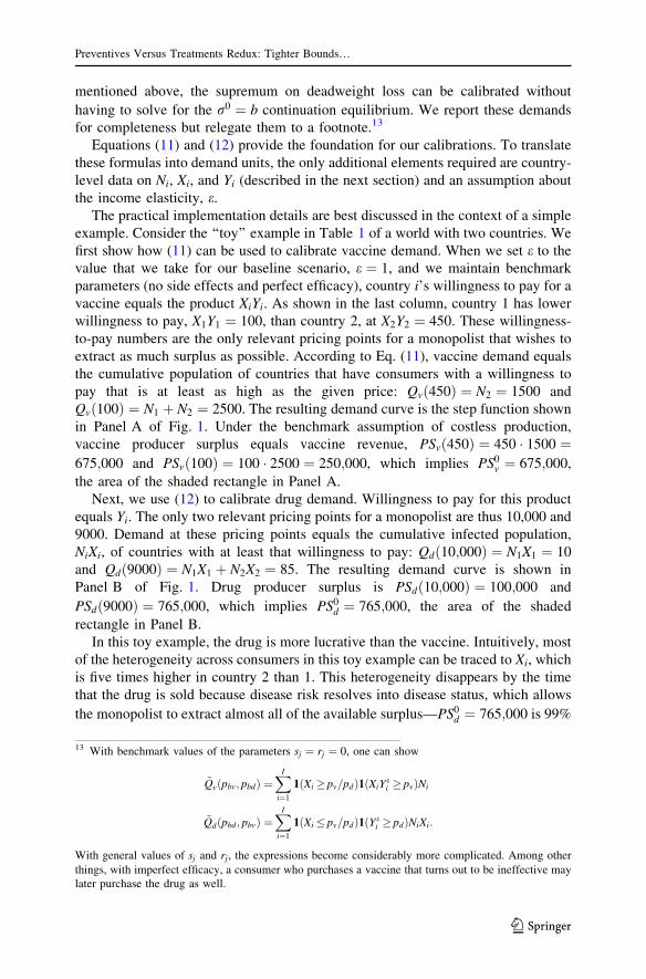
Equations (11) and (12) provide the foundation for our calibrations. To translate
these formulas into demand units, the only additional elements required are country-
level data on Ni, Xi, and Yi (described in the next section) and an assumption about
the income elasticity, e.The practical implementation details are best discussed in the context of a simple
example. Consider the ‘‘toy’’ example in Table 1 of a world with two countries. We
first show how (11) can be used to calibrate vaccine demand. When we set e to the
value that we take for our baseline scenario, e ¼ 1, and we maintain benchmark
parameters (no side effects and perfect efficacy), country i’s willingness to pay for a
vaccine equals the product XiYi. As shown in the last column, country 1 has lower
willingness to pay, X1Y1 ¼ 100, than country 2, at X2Y2 ¼ 450. These willingness-
to-pay numbers are the only relevant pricing points for a monopolist that wishes to
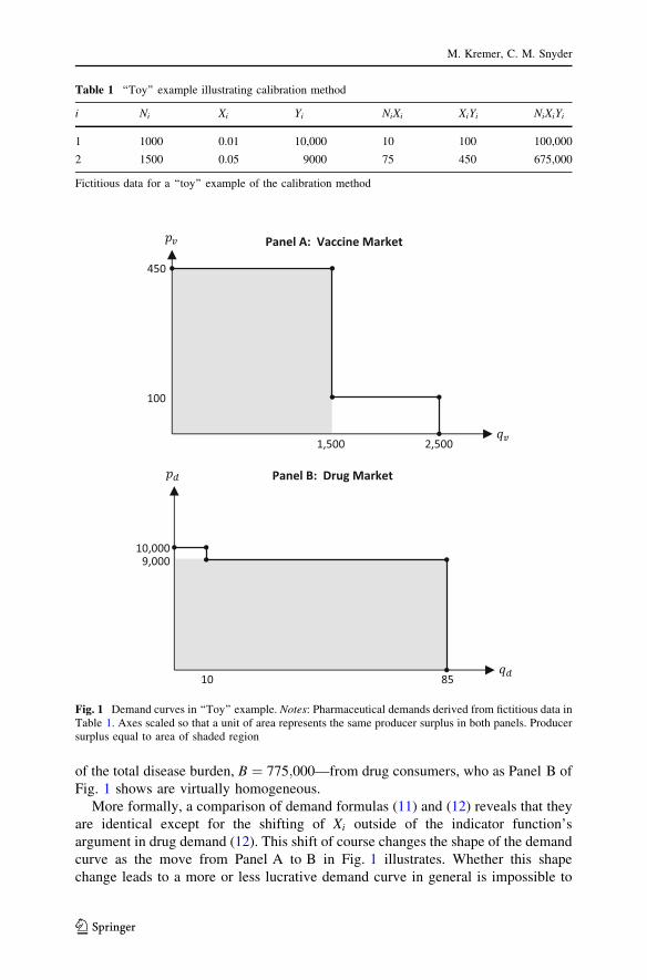
extract as much surplus as possible. According to Eq. (11), vaccine demand equals
the cumulative population of countries that have consumers with a willingness to
pay that is at least as high as the given price: Qvð450Þ ¼ N2 ¼ 1500 and
Qvð100Þ ¼ N1 þ N2 ¼ 2500. The resulting demand curve is the step function shown
in Panel A of Fig. 1. Under the benchmark assumption of costless production,
vaccine producer surplus equals vaccine revenue, PSvð450Þ ¼ 450 � 1500 ¼675;000 and PSvð100Þ ¼ 100 � 2500 ¼ 250;000, which implies PS0
v ¼ 675;000,
the area of the shaded rectangle in Panel A.
Next, we use (12) to calibrate drug demand. Willingness to pay for this product
equals Yi. The only two relevant pricing points for a monopolist are thus 10,000 and
9000. Demand at these pricing points equals the cumulative infected population,
NiXi, of countries with at least that willingness to pay: Qdð10;000Þ ¼ N1X1 ¼ 10
and Qdð9000Þ ¼ N1X1 þ N2X2 ¼ 85. The resulting demand curve is shown in
Panel B of Fig. 1. Drug producer surplus is PSdð10;000Þ ¼ 100;000 and
PSdð9000Þ ¼ 765;000, which implies PS0d ¼ 765;000, the area of the shaded
rectangle in Panel B.
In this toy example, the drug is more lucrative than the vaccine. Intuitively, most
of the heterogeneity across consumers in this toy example can be traced to Xi, which
is five times higher in country 2 than 1. This heterogeneity disappears by the time
that the drug is sold because disease risk resolves into disease status, which allows
the monopolist to extract almost all of the available surplus—PS0d ¼ 765;000 is 99%
13 With benchmark values of the parameters sj ¼ rj ¼ 0, one can show
~Qvðpbv; pbdÞ ¼XI
i¼1
1ðXi � pv=pdÞ1ðXiYei � pvÞNi
~Qdðpbd; pbvÞ ¼XI
i¼1
1ðXi � pv=pdÞ1ðY ei � pdÞNiXi:
With general values of sj and rj, the expressions become considerably more complicated. Among other
things, with imperfect efficacy, a consumer who purchases a vaccine that turns out to be ineffective may
later purchase the drug as well.
Preventives Versus Treatments Redux: Tighter Bounds…
123
of the total disease burden, B ¼ 775;000—from drug consumers, who as Panel B of
Fig. 1 shows are virtually homogeneous.
More formally, a comparison of demand formulas (11) and (12) reveals that they
are identical except for the shifting of Xi outside of the indicator function’s
argument in drug demand (12). This shift of course changes the shape of the demand
curve as the move from Panel A to B in Fig. 1 illustrates. Whether this shape
change leads to a more or less lucrative demand curve in general is impossible to
Table 1 ‘‘Toy’’ example illustrating calibration method
i Ni Xi Yi NiXi XiYi NiXiYi
1 1000 0.01 10,000 10 100 100,000
2 1500 0.05 9000 75 450 675,000
Fictitious data for a ‘‘toy’’ example of the calibration method
450
100
2,5001,500
Panel A: Vaccine Market
10,0009,000
5801
Panel B: Drug Market
Fig. 1 Demand curves in ‘‘Toy’’ example. Notes: Pharmaceutical demands derived from fictitious data inTable 1. Axes scaled so that a unit of area represents the same producer surplus in both panels. Producersurplus equal to area of shaded region
M. Kremer, C. M. Snyder
123
say: cases can be constructed in which q0v [ q0
d, and and other cases can be
constructed in which the reverse inequality holds; the outcomes depend on the joint
distribution of Ni, Xi, and Yi.
More concrete conclusions are available when there is little heterogeneity in Yi.
An immediate corollary of Kremer and Snyder (2015, Proposition 3) is that if
income is homogeneous across countries—if Yi ¼ �Y—and at least two countries
have different positive values of Xi, then q0d [ q0
v . In essence, though incomes are
equal in the two countries, the different disease risks generate different willing-
nesses to pay for a vaccine across the two countries, which (in the absence of price
discrimination) limits the ability of the firm to capture all of the potential surplus; if
a drug rather than a vaccine has been developed, after individuals have realized their
probabilistic disease status, all of the infected individuals are willing (by assumption
of equal incomes) to pay the same amount for the curative drug, which allows the
firm to capture all of the potential surplus. By continuity, this inequality q0d [ q0
v
continues to hold if Yi varies across countries as long as the variance is sufficiently
small. This is the case in the toy example, in which Y1 is only 11% higher than Y2.
We use the same methods to calibrate demand with actual cross-country data as
used here in the toy example. The demand curve will still be a step function but with
finer steps due to the large number of actual countries. As in the toy example, the
number of relevant pricing points for the monopolist is no greater than the number
of countries. Only this manageable number of prices needs to be checked to
compute equilibrium (producer surplus maximizing) prices. Equilibrium prices and
quantities can be combined with the calibrated demand curves to calculate
surpluses, ratios of surpluses to disease burden, and the deadweight loss supremum.
5 Data
This section discusses the data sources for Ni, Xi, and Yi that are used in the
calibrations.
A preliminary question is what year would provide the best snapshot of the
market for HIV pharmaceuticals. While the best year is the current one for most
applications, this is not necessarily the case here.
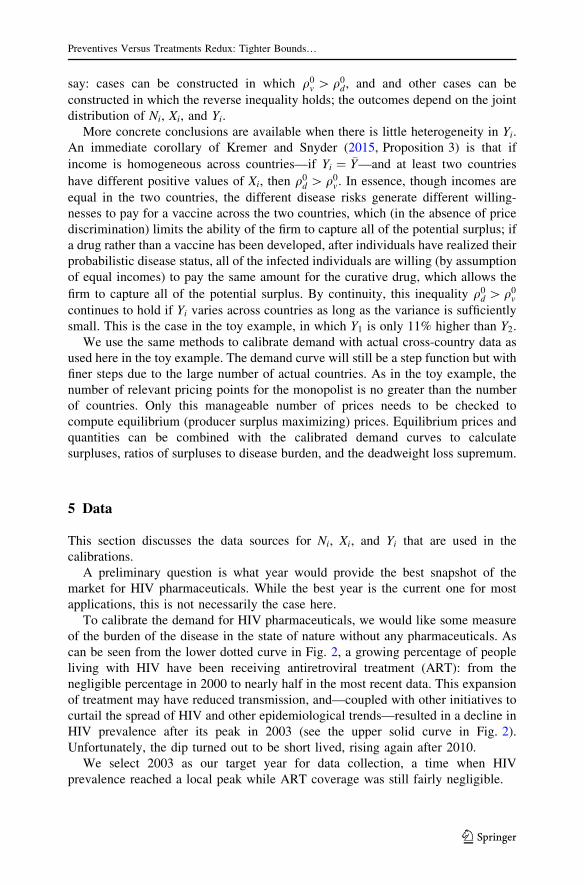
To calibrate the demand for HIV pharmaceuticals, we would like some measure
of the burden of the disease in the state of nature without any pharmaceuticals. As
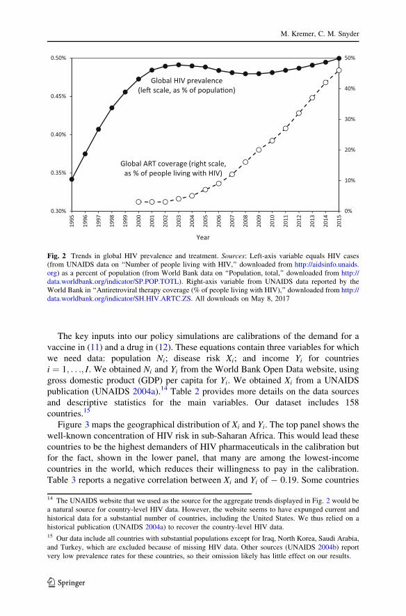
can be seen from the lower dotted curve in Fig. 2, a growing percentage of people
living with HIV have been receiving antiretroviral treatment (ART): from the
negligible percentage in 2000 to nearly half in the most recent data. This expansion
of treatment may have reduced transmission, and—coupled with other initiatives to
curtail the spread of HIV and other epidemiological trends—resulted in a decline in
HIV prevalence after its peak in 2003 (see the upper solid curve in Fig. 2).
Unfortunately, the dip turned out to be short lived, rising again after 2010.
We select 2003 as our target year for data collection, a time when HIV
prevalence reached a local peak while ART coverage was still fairly negligible.
Preventives Versus Treatments Redux: Tighter Bounds…
123
The key inputs into our policy simulations are calibrations of the demand for a
vaccine in (11) and a drug in (12). These equations contain three variables for which
we need data: population Ni; disease risk Xi; and income Yi for countries
i ¼ 1; . . .; I. We obtained Ni and Yi from the World Bank Open Data website, using
gross domestic product (GDP) per capita for Yi. We obtained Xi from a UNAIDS
publication (UNAIDS 2004a).14 Table 2 provides more details on the data sources
and descriptive statistics for the main variables. Our dataset includes 158
countries.15
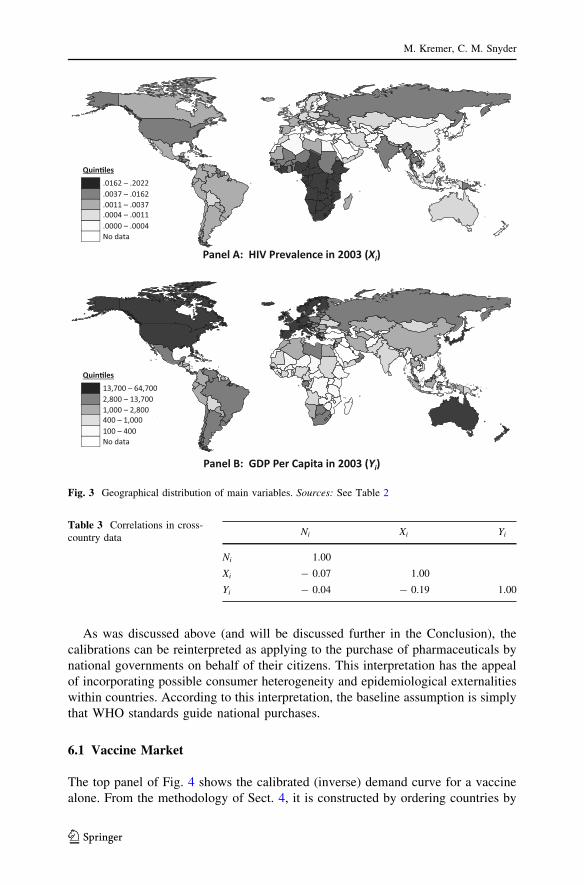
Figure 3 maps the geographical distribution of Xi and Yi. The top panel shows the
well-known concentration of HIV risk in sub-Saharan Africa. This would lead these
countries to be the highest demanders of HIV pharmaceuticals in the calibration but
for the fact, shown in the lower panel, that many are among the lowest-income
countries in the world, which reduces their willingness to pay in the calibration.
Table 3 reports a negative correlation between Xi and Yi of - 0.19. Some countries
0%
10%
20%
30%
40%
50%
0.30%
0.35%
0.40%
0.45%
0.50%
1995
1996
1997
1998
1999
2000
2001
2002
2003
2004
2005
2006
2007
2008
2009
2010
2011
2012
2013
2014
2015
Year
Global HIV prevalence(le� scale, as % of popula�on)
Global ART coverage (right scale,as % of people living with HIV)
Fig. 2 Trends in global HIV prevalence and treatment. Sources: Left-axis variable equals HIV cases(from UNAIDS data on ‘‘Number of people living with HIV,’’ downloaded from http://aidsinfo.unaids.org) as a percent of population (from World Bank data on ‘‘Population, total,’’ downloaded from http://data.worldbank.org/indicator/SP.POP.TOTL). Right-axis variable from UNAIDS data reported by theWorld Bank in ‘‘Antiretroviral therapy coverage (% of people living with HIV),’’ downloaded from http://data.worldbank.org/indicator/SH.HIV.ARTC.ZS. All downloads on May 8, 2017
14 The UNAIDS website that we used as the source for the aggregate trends displayed in Fig. 2 would be
a natural source for country-level HIV data. However, the website seems to have expunged current and
historical data for a substantial number of countries, including the United States. We thus relied on a
historical publication (UNAIDS 2004a) to recover the country-level HIV data.15 Our data include all countries with substantial populations except for Iraq, North Korea, Saudi Arabia,
and Turkey, which are excluded because of missing HIV data. Other sources (UNAIDS 2004b) report
very low prevalence rates for these countries, so their omission likely has little effect on our results.
M. Kremer, C. M. Snyder
123
such as the United States and South Africa are above the median in both Xi and Yiand presumably will be centers of high demand for HIV pharmaceuticals in the
calibration.
6 Calibrations for Baseline Scenario
This section presents calibrations for the baseline scenario in which countries are
heterogeneous in both disease risk Xi and income Yi, the income elasticity is taken to
be e ¼ 1, and the parameters are set at benchmark values cj ¼ sj ¼ rj ¼ 0. Under
these assumptions, a consumer in country i has ex ante willingness to pay XiYi for a
vaccine and ex post willingness to pay Yi for a drug conditional on being infected.
Our analysis of the baseline calibration proceeds by first considering the vaccine
market in isolation and then the drug market in isolation. We then combine these
separate results to compute a comprehensive bound on deadweight loss from
Proposition 2. We conclude the section with an analysis of whether and how
equilibrium in the baseline calibration can be improved with government subsidies.
This baseline specification has some practical appeal beyond its use of round
numbers. Interpret the normalization of harm Hi ¼ 1 as meaning that the
pharmaceutical saves one Disability Adjusted Life Year (DALY). This is roughly
the case for HIV drugs, as taking a year’s course of ARTs roughly extends an
infected person’s life for that year. (Applying this interpretation to an HIV vaccine
requires more care: we either have to assume that a yearly booster shot is needed or,
if the vaccine provides more permanent protection, have to scale up the health
benefit by the discounted flow of DALYs saved.) Under this interpretation, the
baseline assumption that a consumer is willing to pay annual per-capita GDP Yi to
avoid Hi is the same as saying that he or she is willing to spend a year of income to
save a year of life. The standard of the World Health Organization (WHO) is that a
highly cost effective health intervention saves a disability adjusted life year (DALY)
at a cost less than the country’s GDP per capita (see Hutubessy et al. 2003). Thus
our baseline assumption is simply that consumers purchase according to WHO
standards.
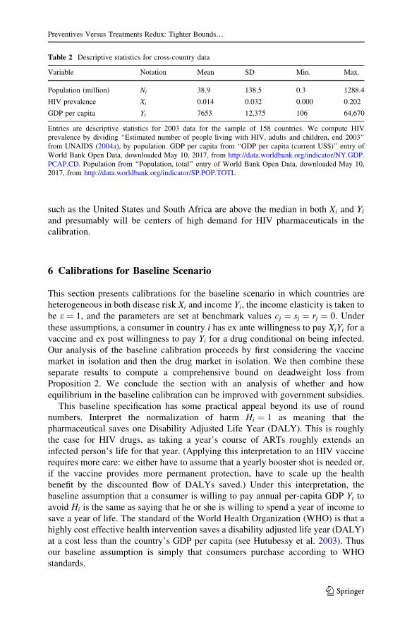
Table 2 Descriptive statistics for cross-country data
Variable Notation Mean SD Min. Max.
Population (million) Ni 38.9 138.5 0.3 1288.4
HIV prevalence Xi 0.014 0.032 0.000 0.202
GDP per capita Yi 7653 12,375 106 64,670
Entries are descriptive statistics for 2003 data for the sample of 158 countries. We compute HIV
prevalence by dividing ‘‘Estimated number of people living with HIV, adults and children, end 2003’’
from UNAIDS (2004a), by population. GDP per capita from ‘‘GDP per capita (current US$)’’ entry of
World Bank Open Data, downloaded May 10, 2017, from http://data.worldbank.org/indicator/NY.GDP.
PCAP.CD. Population from ‘‘Population, total’’ entry of World Bank Open Data, downloaded May 10,
2017, from http://data.worldbank.org/indicator/SP.POP.TOTL
Preventives Versus Treatments Redux: Tighter Bounds…
123
As was discussed above (and will be discussed further in the Conclusion), the
calibrations can be reinterpreted as applying to the purchase of pharmaceuticals by
national governments on behalf of their citizens. This interpretation has the appeal
of incorporating possible consumer heterogeneity and epidemiological externalities
within countries. According to this interpretation, the baseline assumption is simply
that WHO standards guide national purchases.
6.1 Vaccine Market
The top panel of Fig. 4 shows the calibrated (inverse) demand curve for a vaccine
alone. From the methodology of Sect. 4, it is constructed by ordering countries by
700 6470000 1370000 28000 10000 400
Panel B: GDP Per Capita in 2003 (Yi)
No data100 – 400400 – 1,0001,000 – 2,8002,800 – 13,70013,700 – 64,700
Quin�les
162 .193037 .0162011 .0037004 .0011.0004
Panel A: HIV Prevalence in 2003 (Xi)
No data.0000 – .0004.0004 – .0011.0011 – .0037.0037 – .0162.0162 – .2022
Quin�les
Fig. 3 Geographical distribution of main variables. Sources: See Table 2
Table 3 Correlations in cross-
country dataNi Xi Yi
Ni 1.00
Xi - 0.07 1.00
Yi - 0.04 - 0.19 1.00
M. Kremer, C. M. Snyder
123
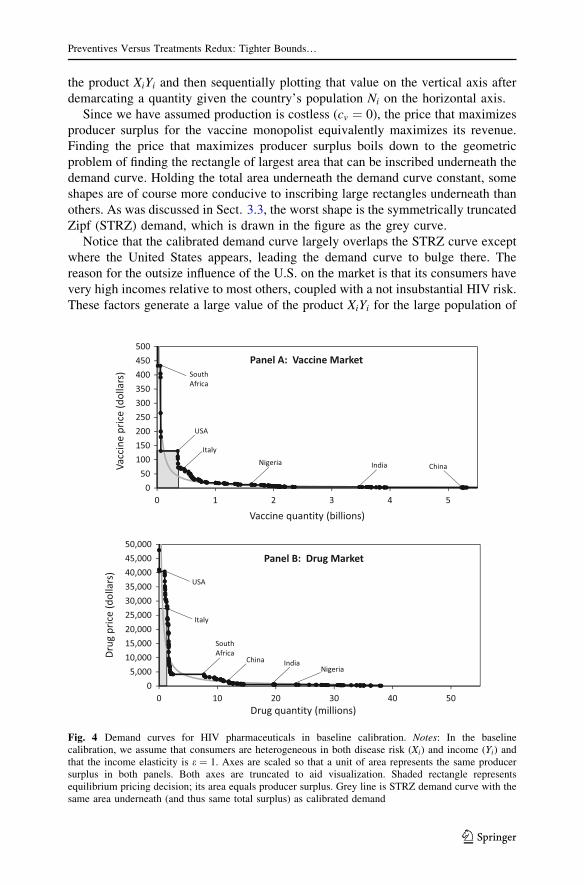
the product XiYi and then sequentially plotting that value on the vertical axis after
demarcating a quantity given the country’s population Ni on the horizontal axis.
Since we have assumed production is costless (cv ¼ 0), the price that maximizes
producer surplus for the vaccine monopolist equivalently maximizes its revenue.
Finding the price that maximizes producer surplus boils down to the geometric
problem of finding the rectangle of largest area that can be inscribed underneath the
demand curve. Holding the total area underneath the demand curve constant, some
shapes are of course more conducive to inscribing large rectangles underneath than
others. As was discussed in Sect. 3.3, the worst shape is the symmetrically truncated
Zipf (STRZ) demand, which is drawn in the figure as the grey curve.
Notice that the calibrated demand curve largely overlaps the STRZ curve except
where the United States appears, leading the demand curve to bulge there. The
reason for the outsize influence of the U.S. on the market is that its consumers have
very high incomes relative to most others, coupled with a not insubstantial HIV risk.
These factors generate a large value of the product XiYi for the large population of
05,00010,00015,00020,00025,00030,00035,00040,00045,00050,000
0 10 20 30 40 50
050
100150200250300350400450500
0 1 2 3 4 5
USA
SouthAfrica
India ChinaNigeria
Italy
Vaccineprice(dollars)
Vaccine quantity (billions)
Panel A: Vaccine Market
Italy
USA
SouthAfrica
IndiaNigeria
ChinaDrug
price(dollars)
Drug quantity (millions)
Panel B: Drug Market
Fig. 4 Demand curves for HIV pharmaceuticals in baseline calibration. Notes: In the baselinecalibration, we assume that consumers are heterogeneous in both disease risk (Xi) and income (Yi) andthat the income elasticity is e ¼ 1. Axes are scaled so that a unit of area represents the same producersurplus in both panels. Both axes are truncated to aid visualization. Shaded rectangle representsequilibrium pricing decision; its area equals producer surplus. Grey line is STRZ demand curve with thesame area underneath (and thus same total surplus) as calibrated demand
Preventives Versus Treatments Redux: Tighter Bounds…
123
U.S. consumers. U.S. consumers are the marginal ones in the calibration: the
producer surplus-maximizing price just induces them to buy and strictly induces
purchases by consumers in Botswana, South Africa, Swaziland, Bahamas, Namibia,
Trinidad and Tobago, and Gabon. While consumers in these other countries are
poorer than in the United States, their extremely high HIV prevalence rates result in
their being higher demanders.
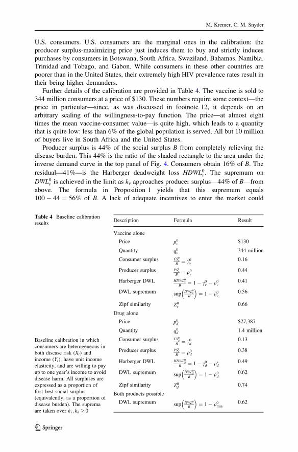
Further details of the calibration are provided in Table 4. The vaccine is sold to
344 million consumers at a price of $130. These numbers require some context—the
price in particular—since, as was discussed in footnote 12, it depends on an
arbitrary scaling of the willingness-to-pay function. The price—at almost eight
times the mean vaccine-consumer value—is quite high, which leads to a quantity
that is quite low: less than 6% of the global population is served. All but 10 million
of buyers live in South Africa and the United States.
Producer surplus is 44% of the social surplus B from completely relieving the
disease burden. This 44% is the ratio of the shaded rectangle to the area under the
inverse demand curve in the top panel of Fig. 4. Consumers obtain 16% of B. The
residual—41%—is the Harberger deadweight loss HDWL0v . The supremum on
DWL0v is achieved in the limit as kv approaches producer surplus—44% of B—from
above. The formula in Proposition 1 yields that this supremum equals
100 � 44 ¼ 56% of B. A lack of adequate incentives to enter the market could
Table 4 Baseline calibration
results
Baseline calibration in which
consumers are heterogeneous in
both disease risk (Xi) and
income (Yi), have unit income
elasticity, and are willing to pay
up to one year’s income to avoid
disease harm. All surpluses are
expressed as a proportion of
first-best social surplus
(equivalently, as a proportion of
disease burden). The suprema
are taken over kv; kd � 0
Description Formula Result
Vaccine alone
Price p0v
$130
Quantity q0v
344 million
Consumer surplus CS0v
B¼ c0
v0.16
Producer surplus PS0v
B¼ q0
v0.44
Harberger DWL HDWL0v
B¼ 1 � c0
v � q0v
0.41
DWL supremum supDWL0
v
B
� �¼ 1 � q0
v0.56
Zipf similarity Z0v
0.66
Drug alone
Price p0d
$27,387
Quantity q0d
1.4 million
Consumer surplus CS0d
B¼ c0
d0.13
Producer surplus PS0d
B¼ q0
d0.38
Harberger DWL HDWL0d
B¼ 1 � c0
d � q�d0.49
DWL supremum supDWL0
d
B
� �¼ 1 � q0
d0.62
Zipf similarity Z0d
0.74
Both products possible
DWL supremum sup DWL0
B
� �¼ 1 � q0
min0.62
M. Kremer, C. M. Snyder
123
dissipate more than half of the social surplus from completely relieving the disease
burden.
Using the formula for the Zipf similarity, Z0j , of the demand for product j
provided by Eq. (9), we obtain Z0v ¼ 0:66: the calibrated vaccine demand curve is
66% similar to the STRZ worst case, in that it generates 66% of the deadweight loss
bound that is generated by the STRZ curve. This measure quantifies the moderately
Zipf similar shape of the calibrated vaccine demand curve.
6.2 Drug Market
We next turn to the market for the drug alone. The calibrated (inverse) demand
curve for a drug is shown in the lower panel of Fig. 4. Given that a drug is only sold
to consumers who contract the disease, it would not be surprising to see it sell at a
much higher price to a much smaller group of consumers than a vaccine. The scale
for drug price on the vertical axis is 100 times that for vaccine price, but the scale
for drug quantity on the horizontal axis is only 1/100 that for vaccine quantity. The
combined scaling of the axes maintains the property that a unit of area reflects the
same revenue and same surplus in both panels.
From the methodology of Sect. 4, the drug demand curve is constructed by
ordering countries in terms of Yi (i.e., GDP per capita), which reflects consumers’ ex
post willingness to pay for a drug conditional on contracting the disease. We then
sequentially plot that value on the vertical axis after demarcating quantity NiXi,
which is equal to the expected number of people in the country who contract the
disease.
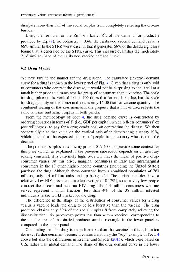
The producer-surplus-maximizing price is $27,400. To provide some context for
this price (which as explained in the previous subsection depends on an arbitrary
scaling constant), it is extremely high: over ten times the mean of positive drug-
consumer values. At this price, marginal consumers in Italy and inframarginal
consumers in the 17 other higher-income countries (including the United States)
purchase the drug. Although these countries have a combined population of 783
million, only 1.4 million units end up being sold. These rich countries have a
relatively low HIV prevalence rate (an average of 0.12%), so relatively few people
contract the disease and need an HIV drug. The 1.4 million consumers who are
served represent a small fraction—less than 4%—of the 38 million infected
individuals in the world market for the drug.
The difference in the shape of the distribution of consumer values for a drug
versus a vaccine leads the drug to be less lucrative than the vaccine. The drug
producer obtains only 38% of the social surplus B from completely relieving the
disease burden—six percentage points less than with a vaccine—corresponding to
the smaller area of the shaded producer-surplus rectangle in the lower panel as
compared to the upper panel.
Our finding that the drug is more lucrative than the vaccine in this calibration
deserves further comment because it contrasts not only the ‘‘toy’’ example in Sect. 4
above but also the calibrations in Kremer and Snyder (2015), which were based on
U.S. rather than global demand. The shape of the drug demand curve in the lower
Preventives Versus Treatments Redux: Tighter Bounds…
123
panel of Fig. 4 is quite close to the STRZ worst case, which is drawn as a grey
curve. Its shape is not conducive to inscribing a rectangle of substantial area
underneath. The drug demand curve is more Zipf similar—Z0d ¼ 0:74—than the
vaccine demand curve—Z0v ¼ 0:66.
The reason that the demand curve for drugs is more Zipf similar than that for
vaccines can be understood from their formulas. As shown in Eq. (11), a consumer’s
willingness to pay for a vaccine depends on the product of disease risk and income:
XiYi. The negative correlation between Xi and Yi shown in Table 3 concentrates
consumer values from the extremes into the middle of the distribution, which leads
to a lucrative bulge in the middle of the vaccine demand curve. From Eq. (12), a
consumer’s willingness to pay for a drug, by contrast, depends only on Yi, so the
negative correlation between Xi and Yi does not induce a bulge in the middle of the
drug demand curve.
Consumers obtain only 13% of B in the drug market. The residual 49% is
Harberger deadweight loss HDWL0d. Nearly half of B is lost because the firm’s most
lucrative strategy is to target the high-income market, which results in the exclusion
of countries like South Africa with a slightly lower income but a tremendous disease
burden.
But HDWL0d understates the potential for deadweight loss from all sources,
DWL0d . Given that the market is not very lucrative, the manufacturer may not have
an incentive to enter at all. The supremum on DWL0d is achieved in the limit as kd
approaches producer surplus—38% of B—from above. Using the formula in
Proposition 1, this supremum equals 100 � 38 ¼ 62% of B.
6.3 Goodness of Fit
The predictions from our vaccine calibration cannot be compared to actual
outcomes since an HIV vaccine has yet to be developed. We can perform the
comparison for the drugs that were developed: ARTs. Our calibration, though
simple, is able to match actual ART price and quantity quite closely. As discussed at
the beginning of Sect. 6, we can interpret $27,400 as the model prediction of
consumer expenditure per DALY for the HIV drug. Freedberg et al. (2001, Table 2)
estimate an actual expenditure per DALY in developed countries of $23,000. If the
$23,000 number reflects price concessions in response to public pressure described
by Reich and Bery (2005), our $27,400 estimate could be close to the counterfactual
price without public pressure.
The calibrated quantity of 1.4 million can be compared to the actual quantity of
1.3 million, computed from Fig. 2 as the reported 4% ART coverage in 2003 times
the 0.5% HIV prevalence times 6.4 billion population. The predicted drug price and
quantity from our calibrations both match the corresponding actual variables
remarkably closely.
M. Kremer, C. M. Snyder
123
6.4 Comprehensive Bound
To obtain a comprehensive bound on deadweight loss, we move from calibrations of
the vaccine and drug market in isolation to a calibration that allows for the
possibility that either or both could be produced. Proposition 2 provides an exact
expression for the supremum on deadweight loss in this comprehensive situation. As
was argued in Sect. 3, it simply equals the greater of the deadweight-loss suprema
from the isolated product markets: the greater of 56 and 62%, and thus equal to
62%, which is reported in the last row of Table 4. This supremum can be
approached in the limit as kv approaches infinity—so that the vaccine market is
certainly non-viable—and as kd approaches 38% of B—so that the drug market falls
just short of the margin of viability.16
6.5 Government Subsidies
Kremer and Snyder (2016) note in Sect. 6 that Harberger deadweight loss can be
highly unstable with a Zipf-similar demand curve. The monopolist may be almost
indifferent between the equilibrium strategy that targets a small segment of high
demand consumers and one that targets the bulk of consumers with a low price. A
small subsidy may be enough to flip the equilibrium from the former to the latter,
which would eliminate most of the Harberger deadweight-loss triangle.
Our baseline calibrations display exactly this property. Consider the calibrated
vaccine market. Less than 6% of potential consumers are served at the high
equilibrium price, which leads to a large Harberger triangle: 41% of B. Introducing
a government subsidy—a per-unit subsidy, which for accounting purposes let us
assume is paid directly to the firm—and gradually raising it in penny increments has
no effect on the equilibrium price or quantity until it reaches $7.69. The next penny
increment to $7.70 causes the firm to cut the price from $130 to zero. This relatively
modest subsidy—just 6% of the pre-subsidy equilibrium price—is enough to
eliminate the Harberger triangle entirely. The subsidy is socially efficient for a wide
range of parameters. Even with a social cost of public funds as high as 1.8 (so
raising $1 of taxes costs society $1.80), social welfare would be higher under the
$7.70 subsidy than in the equilibrium without it. Interestingly, what was intended to
be a subsidy policy with the target of mitigating Harberger deadweight loss ends up
being equivalent to a universal vaccination program.
The effect of a subsidy on the drug market is similar: introducing a government
subsidy (again, a per-unit subsidy that is paid directly to the firm) and gradually
raising it in penny increments has no effect on equilibrium price or quantity until it
reaches $941.34. The next penny increment to $941.35 causes the firm to cut the
price from $27,387 to $265. While a subsidy of over $900 might seem high, since
drug prices are much higher than vaccine prices, in fact the subsidy is only 3% of
16 To see the improvement that Proposition 2 entails over previous results, compare the tight bound of
62% reported here to the bound from Proposition 15 of Kremer and Snyder (2015), equal to
q0max � q0
min ¼ 44 � 38 ¼ 6%. The new bound point-identifies worst-case deadweight loss at 62% of
B. The old bound tells us that the supremum on deadweight loss lies somewhere in the interval between 6
and 100% of B, a fairly uninformative statement in this calibration.
Preventives Versus Treatments Redux: Tighter Bounds…
123
the pre-subsidy equilibrium drug price. Though the subsidy does not fully eliminate
the Harberger triangle, it reduces it to less than 1% of the first-best social surplus
since the 11% of consumers who remain unserved have very low incomes and thus
very low drug demand.17 The subsidy would be socially efficient even if the social
cost of public funds were as high as 2.5.
While the subsidy policy nearly eliminates Harberger deadweight loss condi-
tional on the development of the product, it does little to eliminate the potential for
deadweight loss at the extensive margin regarding whether the product is developed
at all. Intuitively, the subsidies are too small to have much effect on incentives to
enter the market. In the vaccine market, the $7.70 subsidy reduces the supremum on
deadweight loss by just two percentage points, from 56% to 54% of B. In the drug
market, the $941.35 subsidy also reduces the worst-case bound on deadweight loss
by just two percentage points, from 62% to 60%. Substantially improved entry
incentives—thus substantially reducing deadweight loss at the extensive margin—
would call for much larger subsidies.
7 International Price Discrimination
Pharmaceutical manufacturers currently have considerable ability to price discrim-
inate across countries, but there is an active policy debate on whether this ability
should be curtailed—for example, in the contexts of parallel trade for pharmaceu-
ticals within the European Union (Danzon 1998) or re-importation of Canadian
pharmaceuticals in the United States (Pecorino 2002). In contrast to the baseline
calibration, which assumed that the monopolist charges a uniform price across
countries, the calibrations in this section allow for some form of international price
discrimination, whether perfect or within limits set by reference pricing. Comparing
the results across the two sections will allow us to assess the welfare effects of
policies that impede price discrimination.
The results for various scenarios that involve international price discrimination
are presented in Table 5. For brevity, the table just presents relative producer-
surplus ratios q0v and q0
d for each scenario. The producer-surplus ratios are summary
indicators of how lucrative the respective markets for a vaccine and drug are, and
can easily be converted into bounds on deadweight loss using the formula in
Proposition 1. The larger of the two of these gives a comprehensive bound on
deadweight loss by Proposition 2. For reference, the first row of the table repeats the
relative producer-surplus ratio from the baseline calibration, which assumes uniform
pricing.
The second row of the table presents results for a calibration that allows the firm
full freedom to charge different prices across countries. Since our model takes
consumers to be homogeneous within a country, this pricing strategy is equivalent
to perfect price discrimination: it allows the producer to extract 100% of first-best
social surplus regardless of the pharmaceutical it produces. It can extract 100% of
first-best social surplus from the vaccine market by selling to all individuals in
17 Eliminating the Harberger triangle entirely would require almost double the subsidy, $1867.
M. Kremer, C. M. Snyder
123
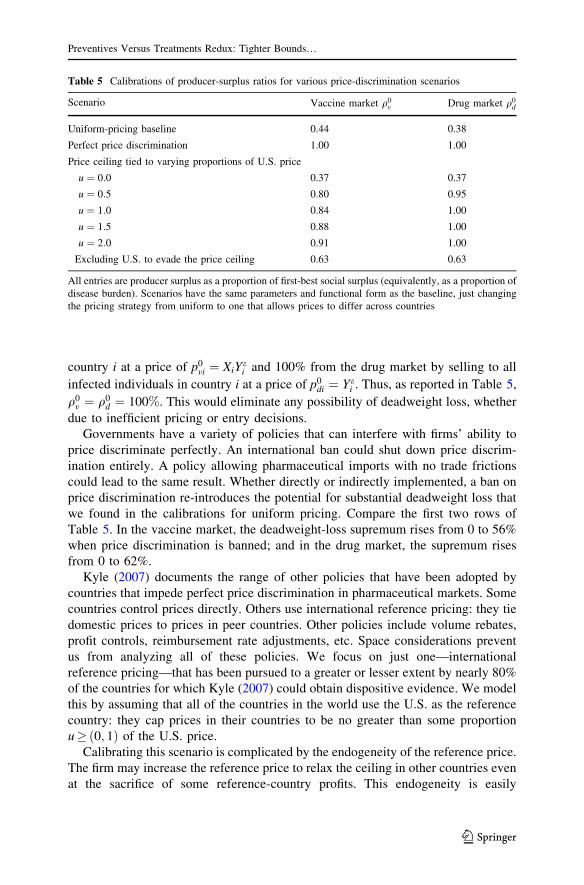
country i at a price of p0vi ¼ XiY
ei and 100% from the drug market by selling to all
infected individuals in country i at a price of p0di ¼ Y e
i . Thus, as reported in Table 5,
q0v ¼ q0
d ¼ 100%. This would eliminate any possibility of deadweight loss, whether
due to inefficient pricing or entry decisions.
Governments have a variety of policies that can interfere with firms’ ability to
price discriminate perfectly. An international ban could shut down price discrim-
ination entirely. A policy allowing pharmaceutical imports with no trade frictions
could lead to the same result. Whether directly or indirectly implemented, a ban on
price discrimination re-introduces the potential for substantial deadweight loss that
we found in the calibrations for uniform pricing. Compare the first two rows of
Table 5. In the vaccine market, the deadweight-loss supremum rises from 0 to 56%
when price discrimination is banned; and in the drug market, the supremum rises
from 0 to 62%.
Kyle (2007) documents the range of other policies that have been adopted by
countries that impede perfect price discrimination in pharmaceutical markets. Some
countries control prices directly. Others use international reference pricing: they tie
domestic prices to prices in peer countries. Other policies include volume rebates,
profit controls, reimbursement rate adjustments, etc. Space considerations prevent
us from analyzing all of these policies. We focus on just one—international
reference pricing—that has been pursued to a greater or lesser extent by nearly 80%
of the countries for which Kyle (2007) could obtain dispositive evidence. We model
this by assuming that all of the countries in the world use the U.S. as the reference
country: they cap prices in their countries to be no greater than some proportion
u�ð0; 1Þ of the U.S. price.
Calibrating this scenario is complicated by the endogeneity of the reference price.
The firm may increase the reference price to relax the ceiling in other countries even
at the sacrifice of some reference-country profits. This endogeneity is easily
Table 5 Calibrations of producer-surplus ratios for various price-discrimination scenarios
Scenario Vaccine market q0v Drug market q0
d
Uniform-pricing baseline 0.44 0.38
Perfect price discrimination 1.00 1.00
Price ceiling tied to varying proportions of U.S. price
u ¼ 0:0 0.37 0.37
u ¼ 0:5 0.80 0.95
u ¼ 1:0 0.84 1.00
u ¼ 1:5 0.88 1.00
u ¼ 2:0 0.91 1.00
Excluding U.S. to evade the price ceiling 0.63 0.63
All entries are producer surplus as a proportion of first-best social surplus (equivalently, as a proportion of
disease burden). Scenarios have the same parameters and functional form as the baseline, just changing
the pricing strategy from uniform to one that allows prices to differ across countries
Preventives Versus Treatments Redux: Tighter Bounds…
123
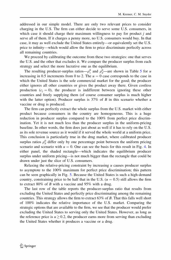
addressed in our simple model. There are only two relevant prices to consider
charging in the U.S. The firm can either decide to serve some U.S. consumers, in
which case it should charge their maximum willingness to pay for product j and
serve all of them. If it charges a penny more, no U.S. consumers would buy. In that
case, it may as well exclude the United States entirely—or equivalently set the U.S.
price to infinity—which would allow the firm to price discriminate perfectly across
all remaining countries.
We proceed by calibrating the outcome from these two strategies: one that serves
the U.S. and the other that excludes it. We compare the producer surplus from each
strategy and select the more lucrative one as the equilibrium.
The resulting producer-surplus ratios—q0v and q0
d—are shown in Table 5 for u
increasing in 0.5 increments from 0 to 2. The u ¼ 0 case corresponds to the case in
which the United States is the sole commercial market for the good; the producer
either ignores all other countries or gives the product away there. Given costless
production (cj ¼ 0), the producer is indifferent between ignoring these other
countries and freely supplying them (of course consumer surplus is much higher
with the latter option). Producer surplus is 37% of B in this scenario whether a
vaccine or drug is produced.
The firm can perfectly extract the whole surplus from the U.S. market with either
product because consumers in the country are homogeneous. This is a huge
reduction in producer surplus compared to the 100% from perfect price discrim-
ination. Yet it is not much less than the producer surplus in the uniform-pricing
baseline. In other words, the firm does just about as well if it has to rely on the U.S.
as its sole revenue source as it would if it served the whole world at a uniform price.
This conclusion is particularly true in the drug market, where calibrated producer
surplus ratios q0d differ only by one percentage point between the uniform pricing
scenario and scenario with u ¼ 0. One can see the basis for this result in Fig. 4. In
either panel, the shaded rectangle—which indicates the equilibrium producer
surplus under uniform pricing—is not much bigger than the rectangle that could be
drawn under just the slice of U.S. consumers.
Relaxing the relative-pricing constraint by increasing u causes producer surplus
to asymptote to the 100% maximum for perfect price discrimination; this pattern
can be seen graphically in Fig. 5. Because the United States is such a high-demand
country, constraining price to be half that in the U.S. (u ¼ 0:5) still allows the firm
to extract 80% of B with a vaccine and 95% with a drug.
The last row of the table reports the producer-surplus ratio that results from
excluding the United States and perfectly price discriminating among the remaining
countries. This strategy allows the firm to extract 63% of B. That this falls well short
of 100% indicates the relative importance of the U.S. market. Comparing the
strategic options that are available to the firm, we see that the producer would prefer
excluding the United States to serving only the United States. However, as long as
the reference price is u� 0:2, the producer earns more from serving than excluding
the United States whether it produces a vaccine or a drug.
M. Kremer, C. M. Snyder
123
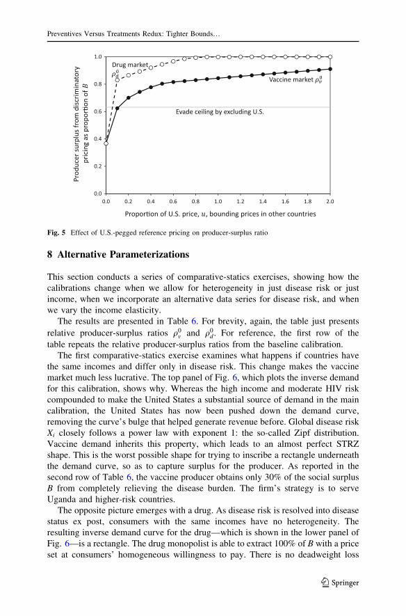
8 Alternative Parameterizations
This section conducts a series of comparative-statics exercises, showing how the
calibrations change when we allow for heterogeneity in just disease risk or just
income, when we incorporate an alternative data series for disease risk, and when
we vary the income elasticity.
The results are presented in Table 6. For brevity, again, the table just presents
relative producer-surplus ratios q0v and q0
d. For reference, the first row of the
table repeats the relative producer-surplus ratios from the baseline calibration.
The first comparative-statics exercise examines what happens if countries have
the same incomes and differ only in disease risk. This change makes the vaccine
market much less lucrative. The top panel of Fig. 6, which plots the inverse demand
for this calibration, shows why. Whereas the high income and moderate HIV risk
compounded to make the United States a substantial source of demand in the main
calibration, the United States has now been pushed down the demand curve,
removing the curve’s bulge that helped generate revenue before. Global disease risk
Xi closely follows a power law with exponent 1: the so-called Zipf distribution.
Vaccine demand inherits this property, which leads to an almost perfect STRZ
shape. This is the worst possible shape for trying to inscribe a rectangle underneath
the demand curve, so as to capture surplus for the producer. As reported in the
second row of Table 6, the vaccine producer obtains only 30% of the social surplus
B from completely relieving the disease burden. The firm’s strategy is to serve
Uganda and higher-risk countries.
The opposite picture emerges with a drug. As disease risk is resolved into disease
status ex post, consumers with the same incomes have no heterogeneity. The
resulting inverse demand curve for the drug—which is shown in the lower panel of
Fig. 6—is a rectangle. The drug monopolist is able to extract 100% of B with a price
set at consumers’ homogeneous willingness to pay. There is no deadweight loss
0.0
0.2
0.4
0.6
0.8
1.0
0.0 0.2 0.4 0.6 0.8 1.0 1.2 1.4 1.6 1.8 2.0
Propor�on of U.S. price, , bounding prices in other countries
Vaccine market
Drug marketProd
ucer
surplusfrom
discrim
inatory
pricingas
prop
or�o
nof
Evade ceiling by excluding U.S.
Fig. 5 Effect of U.S.-pegged reference pricing on producer-surplus ratio
Preventives Versus Treatments Redux: Tighter Bounds…
123
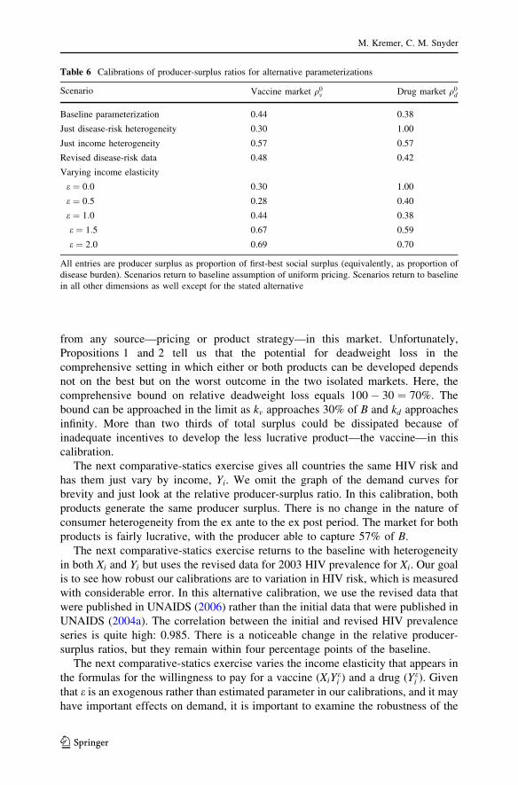
from any source—pricing or product strategy—in this market. Unfortunately,
Propositions 1 and 2 tell us that the potential for deadweight loss in the
comprehensive setting in which either or both products can be developed depends
not on the best but on the worst outcome in the two isolated markets. Here, the
comprehensive bound on relative deadweight loss equals 100 � 30 ¼ 70%. The
bound can be approached in the limit as kv approaches 30% of B and kd approaches
infinity. More than two thirds of total surplus could be dissipated because of
inadequate incentives to develop the less lucrative product—the vaccine—in this
calibration.
The next comparative-statics exercise gives all countries the same HIV risk and
has them just vary by income, Yi. We omit the graph of the demand curves for
brevity and just look at the relative producer-surplus ratio. In this calibration, both
products generate the same producer surplus. There is no change in the nature of
consumer heterogeneity from the ex ante to the ex post period. The market for both
products is fairly lucrative, with the producer able to capture 57% of B.
The next comparative-statics exercise returns to the baseline with heterogeneity
in both Xi and Yi but uses the revised data for 2003 HIV prevalence for Xi. Our goal
is to see how robust our calibrations are to variation in HIV risk, which is measured
with considerable error. In this alternative calibration, we use the revised data that
were published in UNAIDS (2006) rather than the initial data that were published in
UNAIDS (2004a). The correlation between the initial and revised HIV prevalence
series is quite high: 0.985. There is a noticeable change in the relative producer-
surplus ratios, but they remain within four percentage points of the baseline.
The next comparative-statics exercise varies the income elasticity that appears in
the formulas for the willingness to pay for a vaccine (XiYei ) and a drug (Y e
i ). Given
that e is an exogenous rather than estimated parameter in our calibrations, and it may
have important effects on demand, it is important to examine the robustness of the
Table 6 Calibrations of producer-surplus ratios for alternative parameterizations
Scenario Vaccine market q0v Drug market q0
d
Baseline parameterization 0.44 0.38
Just disease-risk heterogeneity 0.30 1.00
Just income heterogeneity 0.57 0.57
Revised disease-risk data 0.48 0.42
Varying income elasticity
e ¼ 0:0 0.30 1.00
e ¼ 0:5 0.28 0.40
e ¼ 1:0 0.44 0.38
e ¼ 1:5 0.67 0.59
e ¼ 2:0 0.69 0.70
All entries are producer surplus as proportion of first-best social surplus (equivalently, as proportion of
disease burden). Scenarios return to baseline assumption of uniform pricing. Scenarios return to baseline
in all other dimensions as well except for the stated alternative
M. Kremer, C. M. Snyder
123
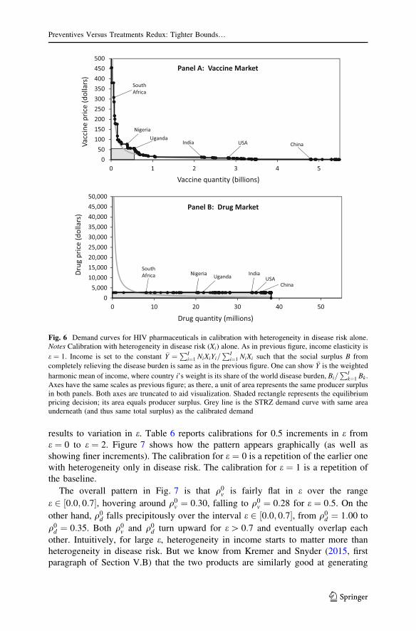
results to variation in e. Table 6 reports calibrations for 0.5 increments in e from
e ¼ 0 to e ¼ 2. Figure 7 shows how the pattern appears graphically (as well as
showing finer increments). The calibration for e ¼ 0 is a repetition of the earlier one
with heterogeneity only in disease risk. The calibration for e ¼ 1 is a repetition of
the baseline.
The overall pattern in Fig. 7 is that q0v is fairly flat in e over the range
e 2 ½0:0; 0:7�, hovering around q0v ¼ 0:30, falling to q0
v ¼ 0:28 for e ¼ 0:5. On the
other hand, q0d falls precipitously over the interval e 2 ½0:0; 0:7�, from q0
d ¼ 1:00 to
q0d ¼ 0:35. Both q0
v and q0d turn upward for e[ 0:7 and eventually overlap each
other. Intuitively, for large e, heterogeneity in income starts to matter more than
heterogeneity in disease risk. But we know from Kremer and Snyder (2015, first
paragraph of Section V.B) that the two products are similarly good at generating
05,000
10,00015,00020,00025,00030,00035,00040,00045,00050,000
0 10 20 30 40 50
050100150200250300350400450500
0 1 2 3 4 5
USA
SouthAfrica
India China
NigeriaUganda
Vaccineprice(dollars)
Vaccine quantity (billions)
Panel A: Vaccine Market
USA
SouthAfrica IndiaNigeria
China
Drug
price(dollars)
Drug quantity (millions)
Panel B: Drug Market
Uganda
Fig. 6 Demand curves for HIV pharmaceuticals in calibration with heterogeneity in disease risk alone.Notes Calibration with heterogeneity in disease risk (Xi) alone. As in previous figure, income elasticity is
e ¼ 1. Income is set to the constant �Y ¼PI
i¼1 NiXiYi=PI
i¼1 NiXi such that the social surplus B from
completely relieving the disease burden is same as in the previous figure. One can show �Y is the weighted
harmonic mean of income, where country i’s weight is its share of the world disease burden, Bi=PI
k¼1 Bk .
Axes have the same scales as previous figure; as there, a unit of area represents the same producer surplusin both panels. Both axes are truncated to aid visualization. Shaded rectangle represents the equilibriumpricing decision; its area equals producer surplus. Grey line is the STRZ demand curve with same areaunderneath (and thus same total surplus) as the calibrated demand
Preventives Versus Treatments Redux: Tighter Bounds…
123
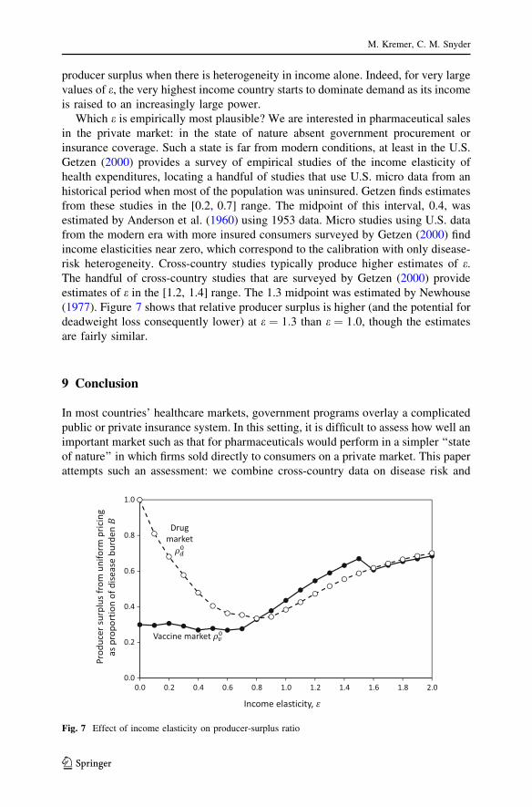
producer surplus when there is heterogeneity in income alone. Indeed, for very large
values of e, the very highest income country starts to dominate demand as its income
is raised to an increasingly large power.
Which e is empirically most plausible? We are interested in pharmaceutical sales
in the private market: in the state of nature absent government procurement or
insurance coverage. Such a state is far from modern conditions, at least in the U.S.
Getzen (2000) provides a survey of empirical studies of the income elasticity of
health expenditures, locating a handful of studies that use U.S. micro data from an
historical period when most of the population was uninsured. Getzen finds estimates
from these studies in the [0.2, 0.7] range. The midpoint of this interval, 0.4, was
estimated by Anderson et al. (1960) using 1953 data. Micro studies using U.S. data
from the modern era with more insured consumers surveyed by Getzen (2000) find
income elasticities near zero, which correspond to the calibration with only disease-
risk heterogeneity. Cross-country studies typically produce higher estimates of e.The handful of cross-country studies that are surveyed by Getzen (2000) provide
estimates of e in the [1.2, 1.4] range. The 1.3 midpoint was estimated by Newhouse
(1977). Figure 7 shows that relative producer surplus is higher (and the potential for
deadweight loss consequently lower) at e ¼ 1:3 than e ¼ 1:0, though the estimates
are fairly similar.
9 Conclusion
In most countries’ healthcare markets, government programs overlay a complicated
public or private insurance system. In this setting, it is difficult to assess how well an
important market such as that for pharmaceuticals would perform in a simpler ‘‘state
of nature’’ in which firms sold directly to consumers on a private market. This paper
attempts such an assessment: we combine cross-country data on disease risk and
0.0
0.2
0.4
0.6
0.8
1.0
0.0 0.2 0.4 0.6 0.8 1.0 1.2 1.4 1.6 1.8 2.0
Income elasticity,
Vaccine market
Drugmarket
Prod
ucer
surplusfrom
unifo
rmpricing
asprop
ortio
nof
diseasebu
rden
Fig. 7 Effect of income elasticity on producer-surplus ratio
M. Kremer, C. M. Snyder
123
income with some simple modeling assumptions to calibrate global pharmaceutical
demand. As a proof of concept, we calibrate demand for an HIV vaccine and drug.
Using these calibrated demands, we can compare how lucrative the products are,
bound deadweight loss from pricing and entry distortions, and simulate the welfare
effects of government policies.
Overall, the analysis reveals a worrisome potential for distortion in global
pharmaceutical markets owing simply to the shape of pharmaceutical demand. The
global demand curves for both a vaccine and a drug are Zipf similar: this is the
shape that was shown in our earlier work (Kremer and Snyder 2015) to have the
greatest potential for deadweight loss at both the intensive/pricing margin (i.e., the
largest Harberger triangle) and the extensive/entry margin (i.e., the largest gap
between private and social incentives to develop the pharmaceutical).
Our baseline calibration assumed that consumers in a country share the same
disease risk (equal to the prevalence of HIV in 2003, when the HIV epidemic was
still growing but before antiretroviral treatments became widespread) and the same
income (equal to per-capital GDP) and have unit income elasticity. These simple
modeling assumptions allowed us to graph the demand curves for a vaccine and a
drug, inscribe the producer-surplus-maximizing rectangle underneath, derive price
and quantity for the simple monopoly equilibrium that we assume, and compute the
deadweight loss.
As a reality check, we compared the predictions from the calibrations to actual
experiences in the case of HIV pharmaceuticals—ARTs—that were available circa
2003. Predictions were close to actual for price ($27,400 vs. $23,000) as well as
quantity (1.4 vs. 1.3 million).
In both the calibrated vaccine and drug markets, the monopolist ends up selling to
a small fraction of high-demand consumers. Deadweight loss from above-cost
pricing in the vaccine market is 41% of the social surplus B from completely
relieving the disease burden, and in the drug market the deadweight loss is 49%.
Potential deadweight loss from inadequate entry incentives is 56% in the vaccine
market and 62% in the drug market. We proved a new proposition showing that this
62% is an exact expression for the deadweight-loss supremum in the comprehensive
case in which either or both products can be developed.
We also ran a suite of calibrations that allow for price discrimination. These
results highlighted the pivotal role that the U.S. plays in global pharmaceutical
demand. In these calibrations the firm finds that targeting just the U.S. is almost as
lucrative as selling to the world at a uniform price. If other countries employ
reference pricing that is pegged to the U.S., for most reasonable scenarios it is more
lucrative for the firm to serve the U.S. and accept the ceiling that this imposes on
other prices than to exclude the U.S. and price discriminate perfectly across the
remaining countries.
The U.S. Department of Commerce (2004) has complained that OECD countries
behave as free riders, relying on the high prices in relatively open U.S. markets to
fund innovation while enjoying low regulatory prices themselves. Our calibrations
suggest that the U.S. would have a pivotal role whether or not other countries
regulated prices, which explains in part why other countries may be emboldened to
free ride.
Preventives Versus Treatments Redux: Tighter Bounds…
123
Our baseline analysis abstracted from the involvement of governments and
insurance companies as well as from epidemiological externalities. These factors
can be integrated back into the analysis under a suitable reinterpretation of the
model: rather than assuming that consumers are homogeneous within each country,
assume instead that national governments (or large national insurers) decide
whether to order a pharmaceutical on behalf of the heterogeneous citizens who are
enrolled their health systems. Assume further that the governments purchase only
pharmaceuticals that satisfy the WHO’s standard of high cost effectiveness: saving a
DALY at a cost that is less than the country’s GDP per capita. Assume finally that
taking either pharmaceutical saves one DALY (so, for example, taking an HIV drug
for a year extends the infected person’s life for a year).
Country i’s pharmaceutical demands are the same under these assumptions as in
our baseline model with direct sales to homogeneous consumers in the country with
disease risk Xi, willingness to pay Yi (given by GDP per capita), harm Hi normalized
to 1, and income elasticity set to e ¼ 1. The model of national-government
purchases can also handle epidemiological externalities, since externalities mostly
flow within a country and would be internalized by the government.18
In future work, we plan to derive a quantitative measure of how pivotal a country
is for innovation incentives. We also plan to enrich the international calibration by
accounting for the heterogeneity of consumers within each country. Kremer and
Snyder (2016) calibrate the global demand for an arbitrary product by assuming a
lognormal distribution of income within each country and using Pinkovskiy and
Sala-i-Martin’s (2009) estimates of the two lognormal parameters for each country.
We are exploring the approach of calibrating global demand for a pharmaceutical by
modeling disease risk and income as bivariate lognormal random variables and
combining surveys and a variety of other data sources to estimate the five requisite
parameters for each country.
Acknowledgements The authors are grateful to the general editor, Lawrence White, the special-issue
editor, Victor Tremblay, and anonymous reviewers for suggestions that substantially improved the paper;
to Margaret Kyle, Paul Novosad, Douglas Staiger, Robert Staiger, Heidi Williams, and seminar
participants at Penn State for insightful comments; and to John Caramichael, Matthew Goodkin-Gold, and
18 Several caveats apply to the model of national-government purchases. First, governments must be
assumed to purchase at a uniform posted international price. If the firm were instead allowed to post
country-specific prices, the outcome would be equivalent to the scenario with perfect price
discrimination. If governments were instead allowed to bargain with the firm, this raises a new scenario
not yet analyzed. It is easy to see that if parties engage in Nash bargaining, they will arrive at the social
optimum. Let a be the firm’s bargaining share. Then the producer-surplus ratios in the bargaining model
would be q0v ¼ q0
d ¼ a. Whether the deadweight-loss supremum is higher or lower in this bargaining
scenario than in the uniform-posted-price baseline depends on a: if a ¼ 0:5, then the deadweight-loss
supremum is lower in the bargaining scenario, but the reverse is true for sufficiently low a. A second
caveat is that the national government’s purchase must be tied to a commitment to universal access for all
citizens—as, for example, Brazil committed to for ARTs in 1996 (Reich and Bery 2005)—rather than
targeting the rich or otherwise higher demand consumers. A third caveat regards the interpretation of
harm relieved by the pharmaceuticals. As noted at the beginning of Sect. 6, if we interpret the Hi ¼ 1
normalization as a year’s course of the drug, which extends life by a year, the parallel interpretation for
the vaccine would involve a booster each year to maintain protection. If the vaccine is assumed to provide
permanent protection, relieved harm would have to be scaled up by the discounted stream of expected
DALYs saved.
M. Kremer, C. M. Snyder
123
Henry Senkfor for excellent research assistance. Caramichael’s and Senkfor’s assistantships were funded
by Dartmouth College’s Presidential Scholars program, which the authors gratefully acknowledge.
Appendix: Proofs of Propositions
Proof of Proposition 1 Assume benchmark values of the parameters. Suppose that
the firm’s only choice is to develop product j or nothing. We will show that the
supremum on relative deadweight loss is bounded by 1 � q0j above and below,
proving the two are equal and thus (6) holds.
A series of steps can be used to bound the supremum from below:
supfkj � 0g
DWL0
B
� �
� limkj#PS0
j
DWL0
B
� �
ð13Þ
¼ limkj#PS0
j
W00
B
� �
ð14Þ
¼ limkj#PS0
j
maxðTS00j � kj; 0ÞB
" #
ð15Þ
¼TS00
j � PS0j
Bð16Þ
¼B� PS0
j
Bð17Þ
¼1 � q0j : ð18Þ
Equation (13) follows since the limit point on the right-hand side is just one element
of the closure of the larger set over which the supremum on the left-hand side is
being taken. Equation (14) holds because nothing is developed in equilibrium in the
limit, which implies W0 ¼ 0 and thus DWL0 ¼ W00 �W0 ¼ W00 in the limit. To
see (15), note that either product j is developed, which yields the social first-best
surplus TS00j � kj, or there is no product, which yields 0. The social optimum
generates the maximum of these two social surpluses. Equation (16) follows from
evaluating the limit, (17) follows from (2), and (18) follows from the definition of
q0j .
We next show that the supremum is bounded from above by 1 � q0j . If W00
j ¼ 0,
then DWL0j ¼ 0� 1 � q0
j , and we are done. So suppose instead that W00j [ 0. We
have the following series of steps:
DWL0 ¼W00 �W0 ð19Þ
¼W00j �W0 ð20Þ
Preventives Versus Treatments Redux: Tighter Bounds…
123
�W00j �P0
j ð21Þ
¼TS00j � kj � ðPS0
j � kjÞ ð22Þ
¼B� PS0j : ð23Þ
Equation (19) holds by definition. Equation (20) holds since W00 ¼ maxð0;W00j Þ ¼
W00j by the maintained assumption that W00
j [ 0. Equation (21) holds since
W0j �P0
j . Equation (22) follows from substituting relevant definitions and (23)
substituting from (2) and canceling terms. Dividing (19)–(23) by B yields
DWL0
B� 1 � q0
j : ð24Þ
Conditions (18) and (24) sandwich the supremum between 1 � q0j above and below,
which yields (6) as an exact equality. h
Proof of Proposition 2 Similar to the previous proof, we will show that the
supremum on relative deadweight loss is bounded by 1 � q0min from above and
below, which proves that the two are equal and thus (7) holds. For concreteness,
suppose throughout the proof that
PS0v �PS0
d: ð25Þ
Arguments establishing the bound for the reverse inequality are similar and omitted
for brevity.
A series of steps can be used to bound the supremum from below:
supfkv;kd � 0g
DWL0
B
� �
� limkv#PS0
v ;kd"1
DWL0
B
� �
ð26Þ
¼ limkv#PS0
v
W00
B
� �
ð27Þ
¼ limkv#PS0
v
maxðW00v ; 0Þ
B
� �
ð28Þ
¼ limkv#PS0
v
maxðTS00v � kv; 0ÞB
� �
ð29Þ
¼1 � q0v ð30Þ
¼1 � q0min: ð31Þ
The arguments for (26) and (27) are similar to those for (13) and (14), respectively.
Equation (28) holds because the socially efficient product strategy cannot involve
M. Kremer, C. M. Snyder
123
development of a drug, alone or together with a vaccine, for sufficiently large kd.
Hence r00 2 fv; ng, which implies that W00 ¼ maxðW00v ; 0Þ. Equation (29) holds by
definition. Equation (30) follows from steps that are similar to (15)–(18), and (31)
holds by assumption (25).
We next bound the supremum from above. We start by establishing that the
following inequality,
DWL0 �B� PS0min; ð32Þ
holds regardless of which value—r00 2 fv; d; b; ng—the socially optimal product
strategy takes on. First consider the trivial case in which r00 ¼ n. Then DWL0 ¼W00 �W0 ¼ 0 since W00 ¼ W0 ¼ 0. But then (32) trivially holds because
B� PS0min � 0 ¼ DWL0.
Next, consider the non-trivial case in which r00 2 fv; d; bg. We can establish the
following series of steps:
DWL0 ¼ W00 �W0 ð33Þ
¼TS00 � kr00 � ðP0 þ CS0Þ ð34Þ
� TS00 � kr00 �P0 ð35Þ
� TS00 � kr00 �P0r00 ð36Þ
¼TS00 � PS0r00 : ð37Þ
¼B� PS0r00 : ð38Þ
Equations (33) and (34) follow from the substitution of the definitions of the rele-
vant variables, and (35) follows from CS0 � 0. Equation (36) holds because the
equilibrium product strategy is the most profitable, implying P0 �P0r00 . Equa-
tion (37) follows from P0r00 ¼ PS0
r00 � kr00 and (38) from (2).
We next show that
PS0r00 �PS0
min ð39Þ
for all r00 2 fv; d; bg. If r00 ¼ v, then PS0r00 ¼ PS0
v �PS0min, which implies that (39)
holds. Similar arguments show that (39) holds if r00 ¼ d. Suppose r00 ¼ b. The
firm can replicate producer surplus from a drug if both products have been devel-
oped by setting pbv ¼ 1 and pbd ¼ p0d. Hence PS0
b �PS0d �PS0
min, which implies
that (39) holds, which completes the proof that (39) holds for all r00 2 fv; d; bg.
We can now complete the proof: combining (38) and (39), we have DWL0 �B�PS0
min for all r00 2 fv; d; bg. Combining this fact with the argument in the text
following (32) implies that (32) holds for all r00 2 fv; d; b; ng. Dividing (32) by B,
Preventives Versus Treatments Redux: Tighter Bounds…
123
DWL0
B� 1 � q0
minð40Þ
for all kv; kd � 0, which implies that
supfkv;kd � 0g
DWL0
B
� �
� 1 � q0min: ð41Þ
Conditions (31) and (41) sandwich the supremum from above and from below at
1 � q0min, which yields (7) as an exact equality. h
References
Acemoglu, D., & Linn, J. (2004). Market size in innovation: Theory and evidence from the
pharmaceutical industry. Quarterly Journal of Economics, 119, 1049–1090.
Anderson, O. W., Collette, P., & Feldman, J. J. (1960). Expenditure patterns for personal health services,
1953 and 1958: Nationwide survey. New York: Health Information Foundation.
Arrow, K. (1962). Economic welfare and the allocation of resources for inventions. In R. Nelson (Ed.),
The rate and direction of inventive activity: Economic and social factors (pp. 609–626). Princeton,
NJ: Princeton University Press.
Brito, D. L., Sheshinski, E., & Intrilligator, M. D. (1991). Externalities and compulsory vaccination.
Journal of Public Economics, 45, 69–90.
Budish, E., Roin, B. N., & Williams, H. L. (2015). Do firms underinvest in long-term research? Evidence
from cancer clinical trials. American Economic Review, 105, 2044–2085.
Chen, F., & Toxvaerd, F. (2014). The economics of vaccination. Journal of Theoretical Biology, 363,
105–117.
Danzon, P. M. (1998). The economics of parallel trade. PharmacoEconomics, 13, 293–304.
Danzon, P. M., & Ketcham, J. D. (2004). Reference pricing of pharmaceuticals for medicare: Evidence
from Germany, the Netherlands, and New Zealand. Frontiers in Health Policy Research, 7, 1–54.
Danzon, P. M., Wang, Y. R., & Wang, L. (2005). The impact of price regulation on the launch delay of
new drugs: Evidence from twenty-five major markets in the 1990s. Health Economics, 14, 269–292.
Finkelstein, A. (2004). Static and dynamic effect of health policy: Evidence from the vaccine industry.
Quarterly Journal of Economics, 119, 527–564.
Francis, P. J. (1997). Dynamic epidemiology and the market for vaccinations. Journal of Public
Economics, 63, 383–406.
Freedberg, K. A., et al. (2001). The cost effectiveness of combination antiretroviral Therapy for HIV
disease. New England Journal of Medicine, 344, 824–831.
Garber, A. M., Jones, C. I., & Romer, P. M. (2006). Insurance and incentives for medical innovation.
Forum for Health Economics & Policy, 9, 1–27.
Geoffard, P.-Y., & Philipson, T. (1997). Disease eradication: Public vs. private vaccination. American
Economic Review, 87, 222–230.
Gersovitz, M. (2003). Births, recoveries, vaccinations, and externalities. In R. Arnott, B. Greenwald, R.
Kanbur, & B. Nalebuff (Eds.), Economics for an imperfect world: Essays in honor of Joseph E.
Stiglitz (pp. 469–483). Cambridge, MA: MIT Press.
Gersovitz, M., & Hammer, J. S. (2004). The economical control of infectious diseases. Economic Journal,
114, 1–27.
Gersovitz, M., & Hammer, J. S. (2005). Tax/subsidy policy toward vector-borne infectious diseases.
Journal of Public Economics, 89, 647–674.
Getzen, T. E. (2000). Health care is an individual necessity and a national luxury: Applying multilevel
decision models to the analysis of health care expenditures. Journal of Health Economics, 19,
259–270.
Harberger, A. C. (1954). Monopoly and resource allocation. American Economic Review, 44, 77–92.
M. Kremer, C. M. Snyder
123
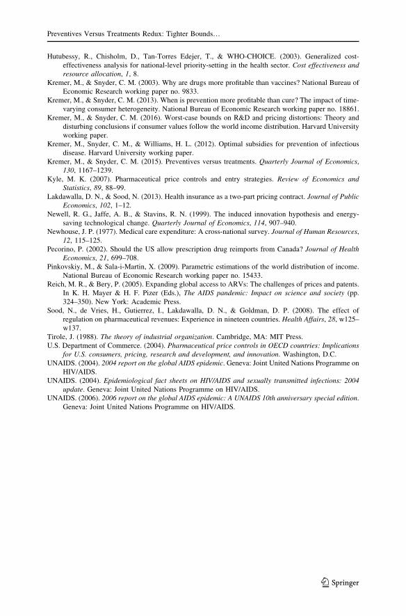
Hutubessy, R., Chisholm, D., Tan-Torres Edejer, T., & WHO-CHOICE. (2003). Generalized cost-
effectiveness analysis for national-level priority-setting in the health sector. Cost effectiveness and
resource allocation, 1, 8.
Kremer, M., & Snyder, C. M. (2003). Why are drugs more profitable than vaccines? National Bureau of
Economic Research working paper no. 9833.
Kremer, M., & Snyder, C. M. (2013). When is prevention more profitable than cure? The impact of time-
varying consumer heterogeneity. National Bureau of Economic Research working paper no. 18861.
Kremer, M., & Snyder, C. M. (2016). Worst-case bounds on R&D and pricing distortions: Theory and
disturbing conclusions if consumer values follow the world income distribution. Harvard University
working paper.
Kremer, M., Snyder, C. M., & Williams, H. L. (2012). Optimal subsidies for prevention of infectious
disease. Harvard University working paper.
Kremer, M., & Snyder, C. M. (2015). Preventives versus treatments. Quarterly Journal of Economics,
130, 1167–1239.
Kyle, M. K. (2007). Pharmaceutical price controls and entry strategies. Review of Economics and
Statistics, 89, 88–99.
Lakdawalla, D. N., & Sood, N. (2013). Health insurance as a two-part pricing contract. Journal of Public
Economics, 102, 1–12.
Newell, R. G., Jaffe, A. B., & Stavins, R. N. (1999). The induced innovation hypothesis and energy-
saving technological change. Quarterly Journal of Economics, 114, 907–940.
Newhouse, J. P. (1977). Medical care expenditure: A cross-national survey. Journal of Human Resources,
12, 115–125.
Pecorino, P. (2002). Should the US allow prescription drug reimports from Canada? Journal of Health
Economics, 21, 699–708.
Pinkovskiy, M., & Sala-i-Martin, X. (2009). Parametric estimations of the world distribution of income.
National Bureau of Economic Research working paper no. 15433.
Reich, M. R., & Bery, P. (2005). Expanding global access to ARVs: The challenges of prices and patents.
In K. H. Mayer & H. F. Pizer (Eds.), The AIDS pandemic: Impact on science and society (pp.
324–350). New York: Academic Press.
Sood, N., de Vries, H., Gutierrez, I., Lakdawalla, D. N., & Goldman, D. P. (2008). The effect of
regulation on pharmaceutical revenues: Experience in nineteen countries. Health Affairs, 28, w125–
w137.
Tirole, J. (1988). The theory of industrial organization. Cambridge, MA: MIT Press.
U.S. Department of Commerce. (2004). Pharmaceutical price controls in OECD countries: Implications
for U.S. consumers, pricing, research and development, and innovation. Washington, D.C.
UNAIDS. (2004). 2004 report on the global AIDS epidemic. Geneva: Joint United Nations Programme on
HIV/AIDS.
UNAIDS. (2004). Epidemiological fact sheets on HIV/AIDS and sexually transmitted infections: 2004
update. Geneva: Joint United Nations Programme on HIV/AIDS.
UNAIDS. (2006). 2006 report on the global AIDS epidemic: A UNAIDS 10th anniversary special edition.
Geneva: Joint United Nations Programme on HIV/AIDS.
Preventives Versus Treatments Redux: Tighter Bounds…
123