Section 1 - Chapter 1Introductory Remarks

R. E. Morrison, Y. Baghzouz, and P. F. Ribeiro,

1.1 Introductionn

This chapter presents an overview of the motivation, importance and previous

developments of probabilistic aspects of harmonics as well as a general introduction of to the

content of the related technical publications. The section considers the early development of

probabilistic methods to model power system harmonic distortion. Initial models were

restricted to the analysis of instantaneous values of current. Direct analytical methods were

originally applied with many simplifications. Initial attempts to use phasor representation of

current also used direct mathematical analysis and simple distributions of amplitude and phase

angle. Direct simulation was applied to test the assumptions used. When power systems

measurement systems became sufficiently powerful the real distributions were measured for

some loads and this enabled a significant increase of accuracy. However, there is still a lack of

knowledge of the distributions that might be used to model the converter harmonic currents.

The chapter concludes by considering the limitations to the application of harmonic analysis in

general and explores the issues that determine whether full spectral analysis should be used.

The application of probabilistic methods to the analysis of power system harmonic

distortion commenced in the late 1960s. Initially, direct mathematical analysis was applied

based on instantaneous values of current from individual harmonic components [1]. Methods

were devised to calculate the probability density function (pdf) for the summation current of

one total harmonic current generated by a number of loads, given the pdfs for the individual

load currents. One of the first attempts to use phasor notation was applied by Rowe [2] in 1974.

He considered the addition of a series of currents modelledmodeled as phasors with random

amplitude and random phase angle. Further, the assumption was made that the amplitude of

each harmonic current was variable with uniform probability density from zero to a peak value

and the phase angle of each current was variable from 0 to 2. Rowe's analysis was limited to

the derivation of the properties of the summation current from a group of distorted loads

connected at one node.

Rowe's analysis was limited to the derivation of the properties of the summation

current from a group of distorted loads connected at one node.

Properties of the summation current were obtained by simplifying the analysis by means of the

a Rayleigh distribution. Unfortunately once such simplifications are applied, flexibility is not

retained and the ability to model a busbarbus bar containing a small number of loads is lost.

However, Rowe was able to show that the highest expected value of current due to a group of

loads could be predicted from the equation:

Where Is is the summation current from individual load currents I11 I22 I33 etc. K is close to

1.5.

Equation (1.1) indicates that the highest expected value of summation current was not

related to the arithmetic sum of all the individual harmonic current amplitudes. This factor was

a major step forward. Also, by introducing the concept of the highest expected current it was

noted that this would be less than the highest possible value of current, namely, which is the

arithmetic sum. It was necessary to define the highest expected current as the value which

would be exceeded for a negligible part of the time. Negligible was taken to be as 1 %per cent.

To calculate this value, the 99th percentile was frequently referred to.

The early analysis depended on assumed probability distributions as well as and

assumed variable ranges. Subsequently, some of the actual probability density functions were

measured in Ref. [3] and found to differ from the assumed pdfs stated above. Simulations were

arranged to derive the cumulative distribution function (CDF) of the summation current for low

order harmonic current components. The estimated CDFs were then compared with the

measured CDFswith reasonable agreement as shown in Figure 1.1 [x].

Using more realistic distributions, simulated statistical values of summation current were

estimated for the substation currents from AC traction supplies.

Figure 1.1 Measured (dotted curve) and calculated (solid curve) CDF of for 5th fifth harmonic current at a traction substation.(continuous line is calculated).

Simulations were arranged to derive the CDF of the summation current for low order

harmonic current components. The estimated CDFs were then compared with measured CDFs

[3] with reasonable agreement reached (Figure 1).

However some shortcomings were noted in relation to the early methods of analysis:

1) There was a lack of knowledge concerning the actual distributions for all but a limited

number of loads.

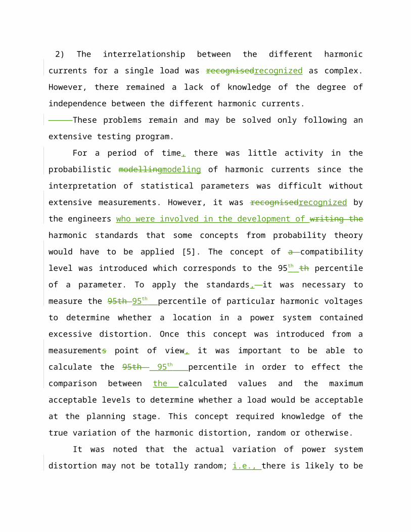
2) The interrelationship between the different harmonic currents for a single load was

recognisedrecognized as complex. However, there remained a lack of knowledge of the degree

of independence between the different harmonic currents.

These problems remain and may be solved only following an extensive testing program.

For a period of time, there was little activity in the probabilistic modellingmodeling of

harmonic currents since the interpretation of statistical parameters was difficult without

extensive measurements. However, it was recognisedrecognized by the engineers who were

involved in the development of writing the harmonic standards that some concepts from

probability theory would have to be applied [5]. The concept of a compatibility level was

introduced which corresponds to the 95th th percentile of a parameter. To apply the standards,

it was necessary to measure the 95th 95th percentile of particular harmonic voltages to

determine whether a location in a power system contained excessive distortion. Once this

concept was introduced from a measurements point of view, it was important to be able to

calculate the 95th 95th percentile in order to effect the comparison between the calculated

values and the maximum acceptable levels to determine whether a load would be acceptable at

the planning stage. This concept required knowledge of the true variation of the harmonic

distortion, random or otherwise.

It was noted that the actual variation of power system distortion may not be totally

random; i.e., there is likely to be a degree of deterministic behaviourbehavior [6].

Measurements made over 24 hours [4] clearly show that a good deal of the variation is due to

the normal daily load fluctuation. This factor complicates the analysis since it provokes a degree

of deterministic behaviourbehavior resulting in a non-stationary process. WhenIn considering a

non-stationary process, it is known that the measured statistics are influenced by the starting

time and the period of time window considered in for the measurement. National power

quality standards normally cover tests made over 24 hours, thus erefore they spanning a period

within which it is not possible to assume that the variation of harmonic distortion is stationary.

The so- called compatibility level is a 95th 95th percentile which applies to the complete 24 hour

period. Therefore, the methods used to evaluate the harmonic levels at the planning stage

must account for the non-stationary nature. To model the non -stationary effects, account must

be taken of the variation of the mean harmonic current with time must be taken into account.

In order to model the complete non-stationary nature of power system distortion, it is

necessary to gain additional knowledge from realistic systems. Measurements are needed to

determine 24 hour trend values to enable suitable models to be provided. The present

harmonic audits may reveal such information [7].

1.2 Spectral Analysis or Harmonic Analysis

Strictly speaking, harmonic analysis may be applied only when currents and voltages are

perfectly steady. This is because the Fourier transform of a perfectly steady distorted waveform

is a series of impulses suggesting that the signal energy is concentrated at a set of discrete

frequencies. Thus, the transfer relationship between current and voltage (impedance) is a

single value at each component of frequency (harmonic); although different impedances at

different frequencies have different values.

When there is variation of the distorted waveform, as shown in Figure 2, the Fourier

transform of the waveform is no longer concentrated at discrete frequencies and but the

energy associated with each harmonic component occupies a particular region within the

frequency band. This is illustrated in Fig. 1.22 which shows the spectrum of an actual time-

varying current waveform [x].

Figure 1.22. Spectrum of a Time-Varying Current Waveform.

If the waveform variation is slow, the frequency range containing 80 per cent of the

energy associated with the signal variation may be restricted. Figure 1.33 shows a typical 5th

harmonic voltage variation on a high voltage (230kV) transmission bus (230kV) during a world

cup soccer event in Brazil [x].

TA limited range of tests have also been carried out to determine the 'spread' of energy

in the frequency domain for a limited set of loads in the past. An analysis carried out for an AC

traction system demonstrated that the 80 per cent energy bandwidth was less than 0.6 Hz for

components up to the 19th harmonic [4].

0,0

0,2

0,4

0,6

0,8

1,0

Hora

5o H

arm

ônic

o (%

)5t

h Vo

ltage

Har

mon

ic D

isto

rtion

(%) 5th Voltage Harmonic Distortion

Start of the game

Period of the game

Hour

Figure 1.33. Fourier transform derived from 5th harmonic voltage variation.

For harmonic analysis to apply, there must be negligible variation of the system

impedance within the frequency range covered by the 80 per cent energy bandwidth. It was

demonstrated in [4] that variation of system impedance over a range of 0.6 Hz is less than 2 per

cent even in unfavorable system circumstances. Thus, harmonic analysis is justified for

applications using some types of locomotive load.

Clearly, further measurement should be carried out to demonstrate that harmonic

analysis is also applicable to other types of loads when changes in current waveform properties

may be more rapid than found in locomotive loads.

1.3 Observations

Probabilistic techniques may be applied to the analysis of harmonic currents from

several sources. However to generalisegeneralize the analysis, there is a need to measure the

PDFs describing harmonic current variation for a variety of loads. There is also a need to

understand the non stationary nature of the current variation in order to predict the

compatibility levels. It is probable that the harmonic audits (currently in progress) could yield

the appropriate information. To determine the compatibility level by calculation, it will be

necessary to determine the non stationary trends within the natural variation of power system

harmonic distortion.

There are circumstances where harmonic analysis does not apply because the rates of

change associated with current variation isare too fast. It is possible to determine the limits to

which harmonic distortion should be applied by considering information transferred into the

frequency domain. A formal approach to understanding this problem might present new insight

into the limits to which harmonic analysis is appropriate.

1.4- Typical Harmonic Variation Signals

To show typical variations of harmonic signals, some recently recorded data at two

different industrial sites, denoted by sites A and B, are presented [x]. Site A represents a

customer's 13.8 kV bus having a rolling mill that is equipped with solid-state 12- pulse DC drives

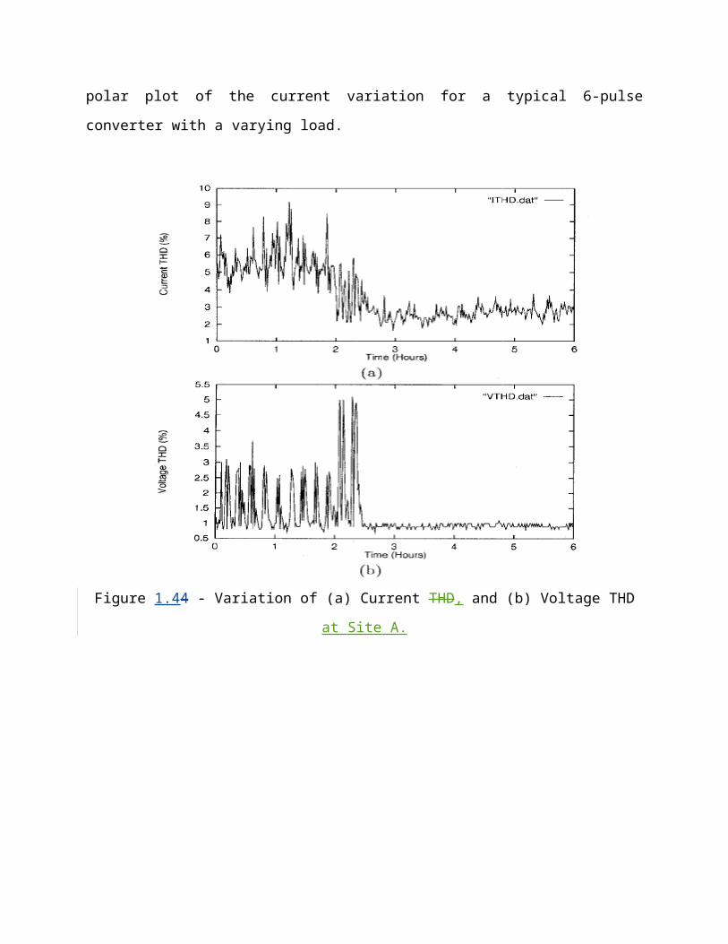
and tuned harmonic filters. Figure 1.44 shows the variations of the current and voltage Total

Harmonic Distortion (THD) of one phase over a 6-hour period. The time interval between

readings is 1 minute, and each data point represents the average FFT for a window size of 16

cycles. It is known that the rolling mill was in operation only during the first 2.5 hours of the

total recording time interval.

Note the reduction in current and voltage harmonic levels at Site A after 2.5 hours of

recording. After this time, the rolling mill was shut-down for maintenance, and only secondary

loads are left operating. The resulting low distortion in current and voltage are caused by

background harmonics.

Site B is another customer's bus loaded with a 66 MW DC arc furnace that is also

equipped with passive harmonic filters. Figure 1.55 (a and b) shows the changes in current and

voltage THDs during a period of one hour, but with one second time interval between readings

and window size of 60 cycles. The sampling rate of the voltage and current signals is 128 times

per cycle at both of the Sites. Finally, Figure 1.665 (c) shows a polar plot of the current

variation for a typical 6-pulse converter with a varying load.

Figure 1.44 - Variation of (a) Current THD, and (b) Voltage THD at Site A.

(c)

Figure 1.55 - Variation of (a) Current THD, and (b) Voltage THD at Site B.

Figure 1.66 - (c) Polar plot of Harmonic Currents of 6-for a six Ppulse Cconverter with a

Vvarying Lload.

Note that the reduction in current and voltage harmonic levels at Site A after 2.5 hours

of recording. After this time, the rolling mill was shut-down for maintenance, and only

secondary loads are left operating. The resulting low distortion in current (THD = 2-3(THD = 1%)

is caused by background harmonics.

Figure 1.55 (a and b) indicates that the voltage THD is quite low although it is known

that the arc furnace load was operating during the one hour time span. This is due to the fact

that the system supplying such a load is quite stiff. Note that the voltage and current THD drop

simultaneously during two periods (4-10 min. and 27-30 min.) whenre the furnace was being

charged. The two bursts of current THD occurring at 10 min. and 30 min. represent furnace

transformer energization after charging.

It is of interest to analyze the effect of current distortion produced by a large nonlinear

load on the distortion of the voltage supplying this load. One graphic way to check for

correlation between these two variables is to plot one as a function of the other, or display a

scatter plot. Figure 1.776 below shows such a plot for Site B. In this particular case, it is clear

that there is no simple relationship between the two THDs. In fact, the correlation coefficient

which measures the strength of a linear relationship is found to be only 0.32.

1.5- Harmonic measurement of time-varying signals

Harmonics are a steady state concept where the waveform to be analyzed is assumed to

repeat itself forever. The most common techniques used in harmonic calculations are based on

the Fast Fourier Transform - a computationally efficient implementation of the Discrete Fourier

Transform (DFT). This algorithm gives accurate results under the following conditions: (i) the

signal is stationary, (ii) the sampling frequency is greater than two times the highest frequency

wit,hin the signal, (iii) the number of periods sampled is an integer, and (iv) the waveform does

not contain frequencies that are non-integer multiples (i.e., inter-harmonics) of the

fundamental frequency.

If the above conditions are satisfied, The FFT algorithm provides accurate results. In such

a case, only a single measurement or "snap-shot" is needed. On the other hand, if inter-

harmonics are present in the signal, multiple periods need to be sampled in order to obtain

accurate harmonic magnitudes.

Figure 1.776 – Scatter Plot of Voltage THD as Function of Current THD at Site B.

In practical situations, however, where the voltage and current distortion levels as well

as their fundamental components are constantly changing in time. Time-variation of individual

harmonics are generated by windowed Fourier transformations (or short-time Fourier

transform), and each harmonic spectrum corresponds to each window section of the

continuous signal. But because deviations often exist within the smallest selected window

length, different windows sizes (i.e., number of cycles included in the FFT) give different

harmonic spectra and adequate window size is a complex issue that is still being debated [13].

Besides hardware-induced errors, e.g., analog-to-digital converters and nonlinearity of potential

and current transformers [14], several software-induced errors also occur when calculating

harmonic levels by direct application of windowed FFTs. These include aliasing, leakage and

picket-fence effect [15].

Aliasing is a consequence of under-sampling, and the problem can be alleviated by anti-

aliasing filters or by increasing the sampling frequency to a value greater than twice the highest

frequency to be evaluated. Leakage refers to apparent spreading of energy from one frequency

into adjacent ones if the number of periods sampled is not an integer. Picket-fence effect

occurs if the analyzed waveform includes a frequency which is not one of the integer harmonic

frequencies of the fundamental. Both leakage and picket-fence effects can be mitigated by

spectral windows.

Several approaches have been proposed in recent years to improve the accuracy of

harmonic magnitudes in time-varying conditions. These include the Kalman filter based analyzer

[15,18], the self-synchronizing Kalman filter approach [17], a scheme based on Parseval's

relation and energy concept [11], and a Fourier linear combiner using adaptive neural networks

[19]. Each one of these methods has advantages and disadvantages, and the search for better

methods continues to be an active research area in signal processing.

1.6 - Characterization of Measured data

When considering charts of harmonic variations with time, one often finds that the

variables contain a large number of irregularities which fail to conform to coherent patterns.

The physical processes which produce these irregularities involve a large number of factors

whose individual effects on harmonic levels cannot be predicted. Due to these elements of

uncertainty, the variations generally have a random character and the only way one can

describe the behavior of such characteristics is in statistical terms which transform a large

volume of data into a compressed and interpretable forms [20].

At times, however, some general patterns can be noticed when examining some of the

charts, thus indicating if that there exists a deterministic component in the recorded signal. In

such cases, a more accurate description is to express the signal as a sum of a deterministic

component and a random component. These descriptions are addressed below with

illustrations using the recorded data (THD) shown in the previous section. These techniques can

also be applied to individual harmonics as well, but such data was not recorded at these Sites.

Statistical Measures

Numerical descriptive measures are the simplest form of representing a set of

measurements. These measures include minimum value, maximum value, average or mean

value, and standard deviation which measures the spread and enables one to construct an

approximate image of the relative distribution of the data set.

Mathematically, let a set of n measurements X i, i =1, ..., n, with minimum value Xmin

maximum value Xmax . The average value and standard deviation are calculated by

The statistical measures for the recorded data at sites A and B are listed in Table 1.1I

below.

Table I1.1: Statistical Measures of Signals Displayed in Figures 1.55 and 1.66.

Given and one might think that the data is spread according to the Gaussian

distribution,

The accuracy of this thought depends on the level of randomness of the signal and

whether it contains a deterministic component. If the signal is completely random, then the

assumption of a gaussian distribution is accurate. On the other hand, if the statistical measures

are derived directly from a signal with a significant deterministic component such as Figure

1.55l(a), then the actual probability distribution is expected to deviate significantly from a

Gaussian distribution as will be seen in the next section. Furthermore, the time factor is

completely lost with such statistical measures. For example, one cannot tell when the

maximum distortion took place within the recording time interval - an important element in

troublelle shooting.

Histograms or Probability Density Functions

Because it is often difficult to determine a priori the best distribution to describe a set of

measurements, a more accurate method is a graph that provides the relative frequency of

occurrence. This type of graph, known as a histogram, shows the portions of the total set of

measurements that fall in various intervals. When scaled do wn such that the total area covered

is equal to unity, the histogram becomes the exact probability density function (pdf) of the

signal.

Figures 1.887 and 1.998 below are the probability density functions corresponding to

the recorded data in Figures 1.44 and 1.55, respectively. Note that pdfs of the current at, Site A

and voltage at Site B contain multiple peaks and cannot be described in terms of the common

distribution functions.

These irregularities are due to the presence of a deterministic component in both

signals. On the other hand, the pdfs in Figs. 1.77(b) and 1.88(a) can be approximated by a

Rayleigh distribution and a Gaussian distrtbution, respectively [21].

Figure 1.887 – Probability Density Function of (a) Current, and (b) Voltage at Site A.

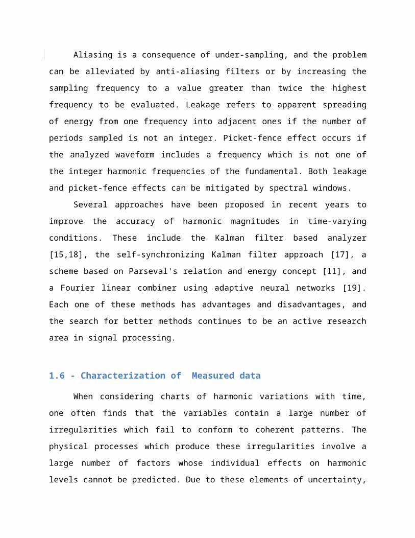
Figure 1.998 - Probability Density Function of (a) Current, and (b) Voltage at Site B.

While histograms represent the measured data in a compressed form and provide more

information than the statistical measures above, they hide information on when some events

took place in time. Although they provide the total time duration during which a harmonic or

distortion level is exceeded, one cannot determine whether such level occuredoccurred in a

continuous fashion or in pulses. Such knowledge is crucial when studying the thermal effects of

harmonics on equipment.

Probability Distribution Functions

A probability distribution function Px(x) represents the same information as a pdf, px(x),

in a different form: Px(x) gives the summation of all the time intervals in which the variable

exceeds a certain level. Mathematically, a distribution function represents the integral of a

density function. One can also use it to express the probability of the event that the observed

variable X is greater than a certain value 2. Since this event is simply the compliment of the

event having probability Px(z), i it follows that

Such probability curves are shown in Ffigure 1.10106 for the recorded signals in figures

1.441 and 1.552. The same advantages and disadvantages as previously mentioned for

histograms apply to the statistical description of data by means of probability distribution

functions.

Statistical Description at Sub-Time Intervals

One way to simplify complex probability density functions or histograms with multiple

peaks and provide more accurate descriptive values, such as those in Figs. 1.887(a) and

1.998(b), and provide more accurate descriptive values is to examine the recorded strip-charts

and search for distinct variations at specific sub-intervals of recording time. Then, one can

calculate the statistical variables for each of these intervals. To illustrate, it can be clearly seen

that the variation in current THD a t site A changes dramatically from one mode to another at t

= 2.5 hours. Hence, two separate histograms can be derived: one for the time period between 0

and 2.5 hours, and the other for the rest of the time, i.e., 2.5 to 6 hours.

One can visualize that this procedure decomposes the histogram in Fig. 1.77(a) into two

distinct ones, each having a single peak, thus easier more easy to describe analytically. The

same procedure can be applied to the voltage THD at Site B. Once again, two distinct modes are

noticed: one corresponds to VTHD less than 0.9% (between 4-10 min. and 27-30 min.), and the

other corresponds to a THD greater than 0.9% for the rest of the time. It should be clear that

the two resulting histograms are equivalent to the two distinct ones shown in Fig. 1.99(b)8(c).

This method preserves the time factor to some extent while providing simple shapes of

probability density functions, but an extra effort in examining the strip-charts is necessary.

Figure 1.10109 - Probability Distribution Functions of (a) Voltages, and (b) Currents shown in

Figures 1.44 and 1.55.

Combined Deterministic/Statistical Description

The recorded signals shown in Figures 1.44 and 1.55 are obviously non-stationary, i.e.,

their probability distribution functions change with the time, due to changes in load conditions

(shutting down the rolling mill at Site A, and charging the arc furnace at Site B). Multiple peaks

on histograms may also show signs of non-stationary signalsity, or the the presence of a

deterministic component within the signal. Theoretical analysis of non-stationary signals is

complex, some of which can be found in Ref. [22]. This section covers an alternative alternative

method to improve the accuracy of the above descriptions by treating the recorded signal as

the sum of a deterministic component XD and a random component XR.

The values of XDo can be extracted by fitting a polynomial function of a certain degree to the

recorded measurements using the method of least squared-error. XR is then defined as the

difference between the actual signal and the deterministic component. It can be shown that the

distribution of XR approaches a normal distribution as the degree of the polynomial function

representing XD increases. In practice, however, it is desirable to work with the simplest model

possible: either a linear of quadratic function.

1.8 Conclusions

This chapter reviewed basic concepts associated with harmonic variations and

measurement of time-varying waveforms, and various ways of describing recorded data

statistically. Statistical measures and histograms are the most commonly used methods. The

shapes of probability densities are found to often have multiple peaks and cannot be

represented by common probability functions. It is further known that these descriptions

completely eliminate the time of occurrence of a certain event. Two methods that alleviate

these problems to some extent, by decomposing the signal or time interval, at the expense of

extra calculations wereare also discussed.

1.9 References

[1] W. G. Sherman, "Summation of harmonics with random phase angles", Proc IEE 1972, 119 (11),

pp. 1643-1648.

[2] N. B. Rowe, "The summation of randomly varying phasors or vectors with particular reference

to harmonic levels", IEE Conf. Ppub.l 110, 1974, pp. 177-181.

[3] R. E. Morrison and A. D. Clark, "A probabilistic representation of harmonic currents in AC

traction systems’ IEE Proc. (b) vol. 131, no. 5, September 1984.

[4] R. E. Morrison, "Measurement analysis and mathematical modelling of harmonic currents in AC

traction systems", Ph.D. thesis, Staffordshire University November 1981.

[5] R E. Morrison, R Carbone, A Testa, G Carpinelli, P Verde, M Fracchia, and L Pierrat, "A review of

probabilistic methods for the analysis of low frequency harmonic distortion", IEE Conf. on EMC

Sept 1994, Pub.l No. 396.

[6] R. E. Morrison and E Duggan, "Prediction of harmonic voltage distortion when a non-linear load

is connected to an already distorted network", IEE Proc. C Vol. 140, 3, 1993.

[7[V Gosbell, D Mannix, D Robinson, and S Perera, "Harmonic survey of an MV distribution

system", Proc. AUPEC, Curtin University, September 2001.

[8] T. Shuter, H. Vollkommer, T. Kirkpatric, "Survey of Harmonic Levels on the American Electric

Power Distribution System," IEEE Trans. Power Delivery, Vol. 4, No.4, 1989, pp. 2204-12.

[9] A. Emanuel, J. Orr, D. Cyganski, E. Gulachenski,"Survey of Harmonic Voltages and Currents at

Distribution Substations," IEEE Trans. Power Delivery, Vol. 6, No. 4, 1991, pp. 1883-90.

[10] J. Arrillaga, A.J.V. Miller, J. Blanco, and L.I. Eguiluz, "Real Time Harmonic Processing of an Arc

Furnace Installation," Proc. IEEE/lCHQPPS VI, Bologna, Italy, Sept. 21-23, 1994, pp. 408-414.

[11] IEEE Std. 519, IEEE Recommended Practices and Requirements for Harmonic Control in

Electric Power Systems, IEEE Press, 1991.

[12] W. Xu, Y. Mansour, C. Siggers, M. El. Hughes, "Developing Utility Harmonic Regulations Based

on IEEE STD 519 - B.C. Hydro's Approach," IEEE Trans. on Power Delivery, Vol. 10, No. 3, 1995,

pp. 137-143.

[13] IEC Sub-Commiitee 77A Report, Dzsturbances Caused by Equizpment Connected to the Publzc

Low-Voltage Supply System: Part 2 - Harmonzcs, 1990 (revised Draft of IEC 555-2).

[14] G. T. Heydt, Power Quality, Star in a Circle Publications, 1991.

[15] A. A. Girgis, W. B. Chang and E. B. Makram, "A Digital Recursive Measurement Scheme for On-

Line Tracking of Power System Harmonics," IEEE Trans. Power DeliDelzvery, Vol. 6, No. 3, 1991,

pp. 1153-60.

[16] H. Ma and A. A. Girgis, "Identification and Tracking of Harmonic Sources in a Power System

Using a Kalman Filter," 1996 EE/PES Winter Meeting, Baltimore, MD, Jan 21-25, 1996, paper No.

96 WM 086-9-PWRD.

[l7] I. Kamwa, R. Grondin and D. McNabb, "On-Line Tracking of Changing Harmonics in Stressed

Power Transmission Systems - Part 11: Application to Hydro-Quebec Network," 1996 IEEE/PES

Winter Meeting, Baltimore, MD, Jan 21-25, 1996, paper No. 96 WM 126-3-PWRD.

[l8] C. S. Moo, Y. N. Chang and P. P. Mok, "A digital Measurement Scheme for Time-Varying

Transient Harmonics," 1994 IEEE/PES Summer Meetizng, paper No. 94 SM 490-3 PWRD.

[19] P. K. Dash, S. K. Patnaik, A. C. Liew, S. Rahman, " An Adaptive Linear Combiner for On-line

Tracking of Power System Harmonics," 1996 IEEE/PES Winter Meeting, Baltimore, MD, Jan 21-

25, 1996, paper No. 96 WM 181-8-PWRS.

[20] G. T. Heydt and E. Gunter, "Post-Measurement Processing of Electric Power Quality Data,"

1996 IEEE/PES Winter Meeting, Baltimore, MD, Jan 21-25, 1996, paper No. 96 WM 063-8-

PWRD.

[21] G. R. Cooper and C. D. McGillem, Probabilistic Methods of Signal and System Analyszs, Holt,

Rinehart and Winston, Inc., 1971.

[22] A. Cavallini, G.C. Montanari and M. Cacciari, "Stochastic Evaluation of Harmonics at Network

Buses," IEEE Trans. on Power Delivery, Vol. 10, No. 3, July 1995, pp. 1606-13.